nag library chapter introduction g02 – correlation … · nag library chapter introduction g02...

NAG Library Chapter Introduction

g02 – Correlation and Regression Analysis

Contents

1 Scope of the Chapter . . . . . . . . . . . . . . . . . . . . . . . . . . . . . . . . . . . . . . . . 3

2 Background to the Problems . . . . . . . . . . . . . . . . . . . . . . . . . . . . . . . . . . 3

2.1 Correlation . . . . . . . . . . . . . . . . . . . . . . . . . . . . . . . . . . . . . . . . . . . . . 3

2.1.1 Aims of correlation analysis . . . . . . . . . . . . . . . . . . . . . . . . . . . . . . . . 32.1.2 Correlation coefficients . . . . . . . . . . . . . . . . . . . . . . . . . . . . . . . . . . . 32.1.3 Partial correlation . . . . . . . . . . . . . . . . . . . . . . . . . . . . . . . . . . . . . . 52.1.4 Robust estimation of correlation coefficients . . . . . . . . . . . . . . . . . . . . . . 62.1.5 Missing values . . . . . . . . . . . . . . . . . . . . . . . . . . . . . . . . . . . . . . . . 6

2.2 Regression . . . . . . . . . . . . . . . . . . . . . . . . . . . . . . . . . . . . . . . . . . . . . . 7

2.2.1 Aims of regression modelling . . . . . . . . . . . . . . . . . . . . . . . . . . . . . . . 72.2.2 Linear regression models . . . . . . . . . . . . . . . . . . . . . . . . . . . . . . . . . . 72.2.3 Fitting the regression model – least-squares estimation . . . . . . . . . . . . . . . . 82.2.4 Regression models and designed experiments . . . . . . . . . . . . . . . . . . . . . 82.2.5 Selecting the regression model . . . . . . . . . . . . . . . . . . . . . . . . . . . . . . 92.2.6 Examining the fit of the model . . . . . . . . . . . . . . . . . . . . . . . . . . . . . . 92.2.7 Computational methods . . . . . . . . . . . . . . . . . . . . . . . . . . . . . . . . . . . 102.2.8 Robust estimation . . . . . . . . . . . . . . . . . . . . . . . . . . . . . . . . . . . . . . 112.2.9 Generalized linear models . . . . . . . . . . . . . . . . . . . . . . . . . . . . . . . . . 122.2.10 Linear mixed effects regression . . . . . . . . . . . . . . . . . . . . . . . . . . . . . . 132.2.11 Ridge regression . . . . . . . . . . . . . . . . . . . . . . . . . . . . . . . . . . . . . . . 142.2.12 Latent variable methods . . . . . . . . . . . . . . . . . . . . . . . . . . . . . . . . . . 14

3 Recommendations on Choice and Use of Available Functions . . . . . . . . 15

3.1 Correlation . . . . . . . . . . . . . . . . . . . . . . . . . . . . . . . . . . . . . . . . . . . . . 15

3.1.1 Product-moment correlation . . . . . . . . . . . . . . . . . . . . . . . . . . . . . . . . 153.1.2 Product-moment correlation with missing values . . . . . . . . . . . . . . . . . . . 153.1.3 Nonparametric correlation . . . . . . . . . . . . . . . . . . . . . . . . . . . . . . . . . 153.1.4 Partial correlation . . . . . . . . . . . . . . . . . . . . . . . . . . . . . . . . . . . . . . 153.1.5 Robust correlation . . . . . . . . . . . . . . . . . . . . . . . . . . . . . . . . . . . . . . 163.1.6 Nearest correlation matrix . . . . . . . . . . . . . . . . . . . . . . . . . . . . . . . . . 16

3.2 Regression . . . . . . . . . . . . . . . . . . . . . . . . . . . . . . . . . . . . . . . . . . . . . . 16

3.2.1 Simple linear regression . . . . . . . . . . . . . . . . . . . . . . . . . . . . . . . . . . 163.2.2 Multiple linear regression – general linear model . . . . . . . . . . . . . . . . . . . 163.2.3 Selecting regression models . . . . . . . . . . . . . . . . . . . . . . . . . . . . . . . . 173.2.4 Residuals . . . . . . . . . . . . . . . . . . . . . . . . . . . . . . . . . . . . . . . . . . . 173.2.5 Robust regression . . . . . . . . . . . . . . . . . . . . . . . . . . . . . . . . . . . . . . 173.2.6 Generalized linear models . . . . . . . . . . . . . . . . . . . . . . . . . . . . . . . . . 183.2.7 Linear mixed effects regression . . . . . . . . . . . . . . . . . . . . . . . . . . . . . . 183.2.8 Ridge regression . . . . . . . . . . . . . . . . . . . . . . . . . . . . . . . . . . . . . . . 183.2.9 Partial Least-squares (PLS) . . . . . . . . . . . . . . . . . . . . . . . . . . . . . . . . 183.2.10 Polynomial regression and nonlinear regression . . . . . . . . . . . . . . . . . . . . 19

4 Index . . . . . . . . . . . . . . . . . . . . . . . . . . . . . . . . . . . . . . . . . . . . . . . . . . . . 19

g02 – Correlation and Regression Analysis Introduction – g02

[NP3678/9] g02.1

5 Functions Withdrawn or Scheduled for Withdrawal . . . . . . . . . . . . . . . 20

6 References . . . . . . . . . . . . . . . . . . . . . . . . . . . . . . . . . . . . . . . . . . . . . . . . 20

Introduction – g02 NAG Library Manual

g02.2 [NP3678/9]

1 Scope of the Chapter

This chapter is concerned with two techniques – correlation analysis and regression modelling – both ofwhich are concerned with determining the inter-relationships among two or more variables.

Other chapters of the NAG C Library which cover similar problems are Chapters e02 and e04. Chaptere02 functions may be used to fit linear models by criteria other than least-squares, and also for polynomialregression; Chapter e04 functions may be used to fit nonlinear models and linearly constrained linearmodels.

2 Background to the Problems

2.1 Correlation

2.1.1 Aims of correlation analysis

Correlation analysis provides a single summary statistic – the correlation coefficient – describing thestrength of the association between two variables. The most common types of association which areinvestigated by correlation analysis are linear relationships, and there are a number of forms of linearcorrelation coefficients for use with different types of data.

2.1.2 Correlation coefficients

The (Pearson) product-moment correlation coefficients measure a linear relationship, while Kendall’s tauand Spearman’s rank order correlation coefficients measure monotonicity only. All three coefficients rangefrom �1:0 to þ1:0. A coefficient of zero always indicates that no linear relationship exists; a þ1:0coefficient implies a ‘perfect’ positive relationship (i.e., an increase in one variable is always associatedwith a corresponding increase in the other variable); and a coefficient of �1:0 indicates a ‘perfect’ negativerelationship (i.e., an increase in one variable is always associated with a corresponding decrease in theother variable).

Consider the bivariate scattergrams in Figure 1: (a) and (b) show strictly linear functions for which thevalues of the product-moment correlation coefficient, and (since a linear function is also monotonic) bothKendall’s tau and Spearman’s rank order coefficients, would be þ1:0 and �1:0 respectively. However,though the relationships in figures (c) and (d) are respectively monotonically increasing and monotonicallydecreasing, for which both Kendall’s and Spearman’s nonparametric coefficients would be þ1:0 (in (c))and �1:0 (in (d)), the functions are nonlinear so that the product-moment coefficients would not take such‘perfect’ extreme values. There is no obvious relationship between the variables in figure (e), so all threecoefficients would assume values close to zero, while in figure (f) though there is an obvious parabolicrelationship between the two variables, it would not be detected by any of the correlation coefficientswhich would again take values near to zero; it is important therefore to examine scattergrams as well as thecorrelation coefficients.

In order to decide which type of correlation is the most appropriate, it is necessary to appreciate thedifferent groups into which variables may be classified. Variables are generally divided into four types ofscales: the nominal scale, the ordinal scale, the interval scale, and the ratio scale. The nominal scale isused only to categorise data; for each category a name, perhaps numeric, is assigned so that two differentcategories will be identified by distinct names. The ordinal scale, as well as categorising the observations,orders the categories. Each category is assigned a distinct identifying symbol, in such a way that the orderof the symbols corresponds to the order of the categories. (The most common system for ordinal variablesis to assign numerical identifiers to the categories, though if they have previously been assigned alphabeticcharacters, these may be transformed to a numerical system by any convenient method which preserves theordering of the categories.) The interval scale not only categorises and orders the observations, but alsoquantifies the comparison between categories; this necessitates a common unit of measurement and anarbitrary zero-point. Finally, the ratio scale is similar to the interval scale, except that it has an absolute(as opposed to arbitrary) zero-point.


[NP3678/9] g02.3

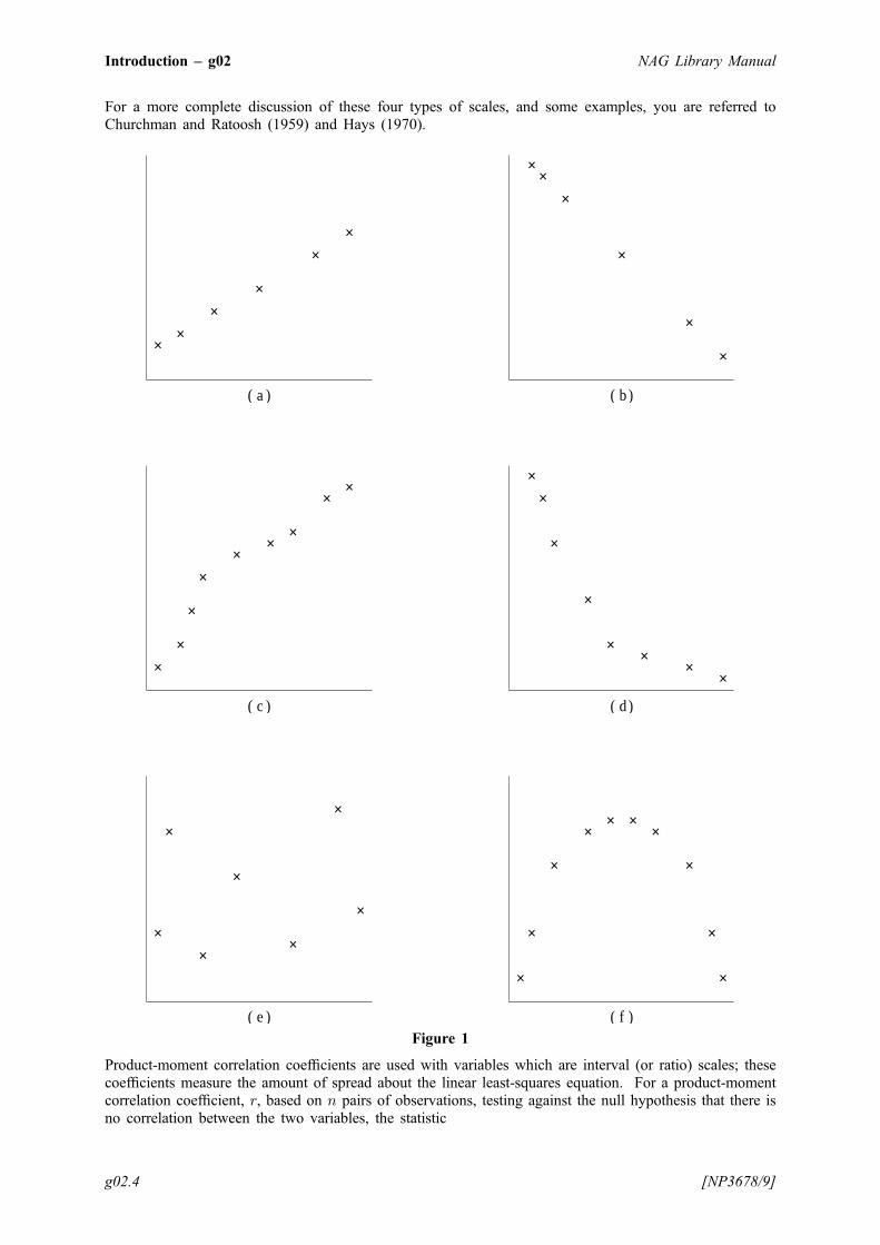
For a more complete discussion of these four types of scales, and some examples, you are referred toChurchman and Ratoosh (1959) and Hays (1970).

( a )

××

××

××

( c )

××

×

××

××

××

( e )

×

×

×

×

×

×

×

( b )

××

×

×

×

×

( d )

××

×

×

××

××

( f )

×

×

×

×× ×

×

×

×

×

Figure 1

Product-moment correlation coefficients are used with variables which are interval (or ratio) scales; thesecoefficients measure the amount of spread about the linear least-squares equation. For a product-momentcorrelation coefficient, r, based on n pairs of observations, testing against the null hypothesis that there isno correlation between the two variables, the statistic


g02.4 [NP3678/9]

r

ffiffiffiffiffiffiffiffiffiffiffiffiffin� 2

1� r2

rhas a Student’s t-distribution with n� 2 degrees of freedom; its significance can be tested accordingly.

Ranked and ordinal scale data are generally analysed by nonparametric methods – usually eitherSpearman’s or Kendall’s tau rank-order correlation coefficients, which, as their names suggest, operatesolely on the ranks, or relative orders, of the data values. Interval or ratio scale variables may also bevalidly analysed by nonparametric methods, but such techniques are statistically less powerful than aproduct-moment method. For a Spearman rank-order correlation coefficient, R, based on n pairs ofobservations, testing against the null hypothesis that there is no correlation between the two variables, forlarge samples the statistic

R

ffiffiffiffiffiffiffiffiffiffiffiffiffiffin� 2

1�R2

rhas approximately a Student’s t-distribution with n� 2 degrees of freedom, and may be treatedaccordingly. (This is similar to the product-moment correlation coefficient, r, see above.) Kendall’s taucoefficient, based on n pairs of observations, has, for large samples, an approximately Normal distributionwith mean zero and standard deviation ffiffiffiffiffiffiffiffiffiffiffiffiffiffiffiffiffiffiffiffiffi

4nþ 10

9n n� 1ð Þ

swhen tested against the null hypothesis that there is no correlation between the two variables; thecoefficient should therefore be divided by this standard deviation and tested against the standard Normaldistribution, N 0; 1ð Þ.When the number of ordinal categories a variable takes is large, and the number of ties is relatively small,Spearman’s rank-order correlation coefficients have advantages over Kendall’s tau; conversely, when thenumber of categories is small, or there are a large number of ties, Kendall’s tau is usually preferred. Thuswhen the ordinal scale is more or less continuous, Spearman’s rank-order coefficients are preferred,whereas Kendall’s tau is used when the data is grouped into a smaller number of categories; both measuresdo however include corrections for the occurrence of ties, and the basic concepts underlying the twocoefficients are quite similar. The absolute value of Kendall’s tau coefficient tends to be slightly smallerthan Spearman’s coefficient for the same set of data.

There is no authoritative dictum on the selection of correlation coefficients – particularly on theadvisability of using correlations with ordinal data. This is a matter of discretion for you.

2.1.3 Partial correlation

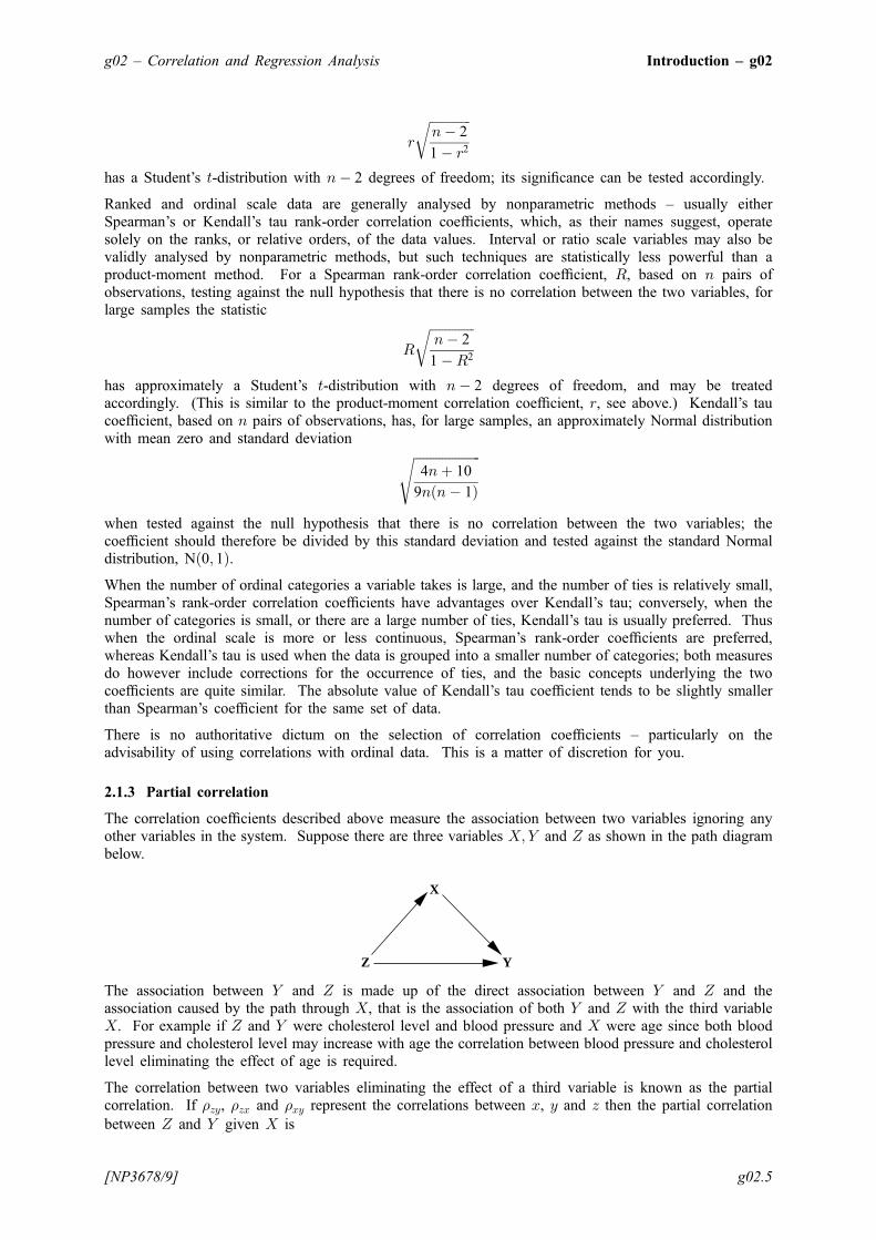
The correlation coefficients described above measure the association between two variables ignoring anyother variables in the system. Suppose there are three variables X; Y and Z as shown in the path diagrambelow.

X

Z Y

The association between Y and Z is made up of the direct association between Y and Z and theassociation caused by the path through X, that is the association of both Y and Z with the third variableX. For example if Z and Y were cholesterol level and blood pressure and X were age since both bloodpressure and cholesterol level may increase with age the correlation between blood pressure and cholesterollevel eliminating the effect of age is required.

The correlation between two variables eliminating the effect of a third variable is known as the partialcorrelation. If �zy, �zx and �xy represent the correlations between x, y and z then the partial correlationbetween Z and Y given X is


[NP3678/9] g02.5

�zy � �zx�xyffiffiffiffiffiffiffiffiffiffiffiffiffiffiffiffiffiffiffiffiffiffiffiffiffiffiffiffiffiffiffiffiffiffiffiffiffi1� �2zxð Þ 1� �2xy

� �q .

The partial correlation is then estimated by using product-moment correlation coefficients.

In general, let a set of variables be partitioned into two groups Y and X with ny variables in Y and nxvariables in X and let the variance-covariance matrix of all ny þ nx variables be partitioned into

�xx �yx

�xy �yy

� �.

Then the variance-covariance of Y conditional on fixed values of the X variables is given by

�yjx ¼ �yy ��yx��1xx�xy.

The partial correlation matrix is then computed by standardizing �yjx.

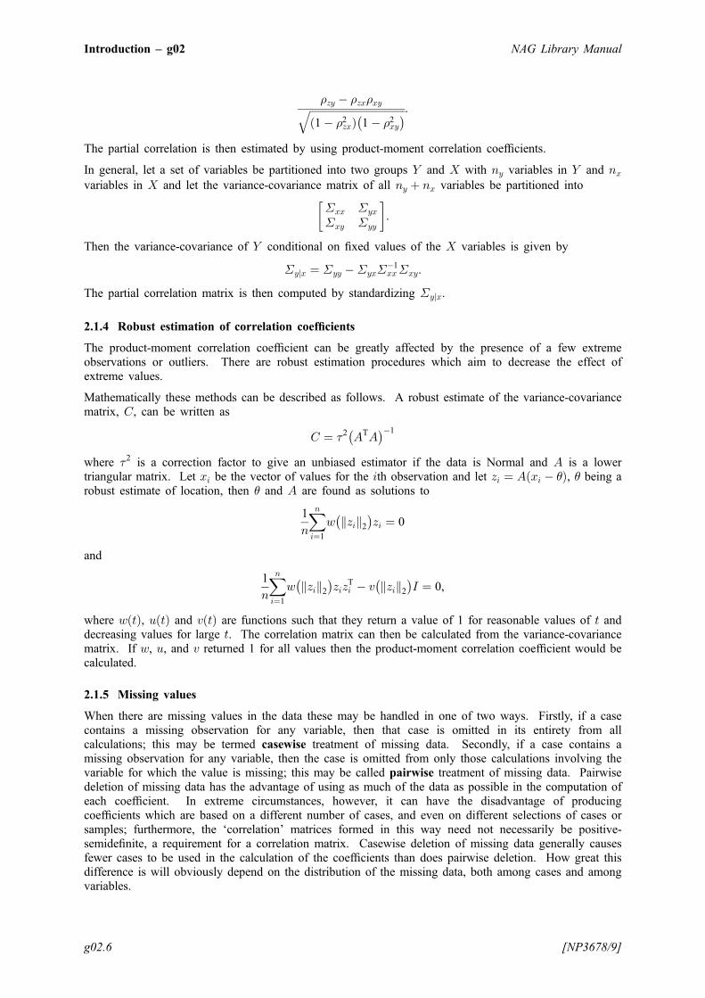
2.1.4 Robust estimation of correlation coefficients

The product-moment correlation coefficient can be greatly affected by the presence of a few extremeobservations or outliers. There are robust estimation procedures which aim to decrease the effect ofextreme values.

Mathematically these methods can be described as follows. A robust estimate of the variance-covariancematrix, C, can be written as

C ¼ �2 ATA� ��1

where �2 is a correction factor to give an unbiased estimator if the data is Normal and A is a lowertriangular matrix. Let xi be the vector of values for the ith observation and let zi ¼ A xi � �ð Þ, � being arobust estimate of location, then � and A are found as solutions to

1

n

Xni¼1

w zik k2� �

zi ¼ 0

and

1

n

Xni¼1

w zik k2� �

zizTi � v zik k2

� �I ¼ 0,

where w tð Þ, u tð Þ and v tð Þ are functions such that they return a value of 1 for reasonable values of t anddecreasing values for large t. The correlation matrix can then be calculated from the variance-covariancematrix. If w, u, and v returned 1 for all values then the product-moment correlation coefficient would becalculated.

2.1.5 Missing values

When there are missing values in the data these may be handled in one of two ways. Firstly, if a casecontains a missing observation for any variable, then that case is omitted in its entirety from allcalculations; this may be termed casewise treatment of missing data. Secondly, if a case contains amissing observation for any variable, then the case is omitted from only those calculations involving thevariable for which the value is missing; this may be called pairwise treatment of missing data. Pairwisedeletion of missing data has the advantage of using as much of the data as possible in the computation ofeach coefficient. In extreme circumstances, however, it can have the disadvantage of producingcoefficients which are based on a different number of cases, and even on different selections of cases orsamples; furthermore, the ‘correlation’ matrices formed in this way need not necessarily be positive-semidefinite, a requirement for a correlation matrix. Casewise deletion of missing data generally causesfewer cases to be used in the calculation of the coefficients than does pairwise deletion. How great thisdifference is will obviously depend on the distribution of the missing data, both among cases and amongvariables.


g02.6 [NP3678/9]

Pairwise treatment does therefore use more information from the sample, but should not be used withoutcareful consideration of the location of the missing observations in the data matrix, and the consequenteffect of processing the missing data in that fashion.

Consider a matrix with elements given by the product-moment correlation of pairs of variables, with anymissing values treated in the pairwise sense. Such a matrix may not be positive semi-definite, andtherefore not a valid correlation matrix. However, a valid correlation matrix can be calculated that is insome sense ‘close’ to the original. One measure of closeness is the Frobenius norm. This valid correlationmatrix is the solution to the nearest correlation matrix problem.

2.2 Regression

2.2.1 Aims of regression modelling

In regression analysis the relationship between one specific random variable, the dependent or responsevariable, and one or more known variables, called the independent variables or covariates, is studied.This relationship is represented by a mathematical model, or an equation, which associates the dependentvariable with the independent variables, together with a set of relevant assumptions. The independentvariables are related to the dependent variable by a function, called the regression function, whichinvolves a set of unknown parameters. Values of the arguments which give the best fit for a given set ofdata are obtained; these values are known as the estimates of the arguments.

The reasons for using a regression model are twofold. The first is to obtain a description of therelationship between the variables as an indicator of possible causality. The second reason is to predictthe value of the dependent variable from a set of values of the independent variables. Accordingly, themost usual statistical problems involved in regression analysis are:

(i) to obtain best estimates of the unknown regression arguments;

(ii) to test hypotheses about these arguments;

(iii) to determine the adequacy of the assumed model; and

(iv) to verify the set of relevant assumptions.

2.2.2 Linear regression models

When the regression model is linear in the arguments (but not necessarily in the independent variables),then the regression model is said to be linear; otherwise the model is classified as nonlinear.

The most elementary form of regression model is the simple linear regression of the dependent variable,Y , on a single independent variable, x, which takes the form

E Yð Þ ¼ �0 þ �1x ð1Þwhere E Yð Þ is the expected or average value of Y and �0 and �1 are the arguments whose values are to beestimated, or, if the regression is required to pass through the origin (i.e., no constant term),

E Yð Þ ¼ �1x ð2Þwhere �1 is the only unknown argument.

An extension of this is multiple linear regression in which the dependent variable, Y , is regressed on thep (p > 1) independent variables, x1; x2; . . . ; xp, which takes the form

E Yð Þ ¼ �0 þ �1x1 þ �2x2 þ � � � þ �pxp ð3Þ

where �1; �2; . . . ; �p and �0 are the unknown arguments.

A special case of multiple linear regression is polynomial linear regression, in which the p independent

variables are in fact powers of the same single variable x (i.e., xj ¼ xj, for j ¼ 1; 2; . . . ; p).

In this case, the model defined by (3) becomes

E Yð Þ ¼ �0 þ �1xþ �2x2 þ � � � þ �px

p. ð4Þ

There are a great variety of nonlinear regression models; one of the most common is exponentialregression, in which the equation may take the form


[NP3678/9] g02.7

E Yð Þ ¼ aþ becx. ð5ÞIt should be noted that equation (4) represents a linear regression, since even though the equation is notlinear in the independent variable, x, it is linear in the arguments �0; �1; �2; . . . :; �p, whereas the regressionmodel of equation (5) is nonlinear, as it is nonlinear in the arguments (a, b and c).

2.2.3 Fitting the regression model – least-squares estimation

The method used to determine values for the arguments is, based on a given set of data, to minimize thesums of squares of the differences between the observed values of the dependent variable and the valuespredicted by the regression equation for that set of data – hence the term least-squares estimation. Forexample, if a regression model of the type given by equation (3), namely

E Yð Þ ¼ �0x0 þ �1x1 þ �2x2 þ � � � þ �pxp,

where x0 ¼ 1 for all observations, is to be fitted to the n data points

x01; x11; x21; . . . ; xp1; y1� �x02; x12; x22; . . . ; xp2; y2� �

..

.

x0n; x1n; x2n; . . . ; xpn; yn� � ð6Þ

such that

yi ¼ �0x0 þ �1x1i þ �2x2i þ � � � þ �pxpi þ ei, i ¼ 1; 2; . . . ; n

where ei are unknown independent random errors with E eið Þ ¼ 0 and var eið Þ ¼ �2, �2 being a constant,then the method used is to calculate the estimates of the regression arguments �0; �1; �2; . . . ; �p byminimizing Xn

i¼1

e2i . ð7Þ

If the errors do not have constant variance, i.e.,

var eið Þ ¼ �2i ¼�2

wi

then weighted least-squares estimation is used in whichXni¼1

wie2i

is minimized. For a more complete discussion of these least-squares regression methods, and details of themathematical techniques used, see Draper and Smith (1985) or Kendall and Stuart (1973).

2.2.4 Regression models and designed experiments

One application of regression models is in the analysis of experiments. In this case the model relates thedependent variable to qualitative independent variables known as factors. Factors may take a number ofdifferent values known as levels. For example, in an experiment in which one of four different treatmentsis applied, the model will have one factor with four levels. Each level of the factor can be represented bya dummy variable taking the values 0 or 1. So in the example there are four dummy variables xj, forj ¼ 1; 2; 3; 4 such that:

xij ¼ 1 if the ith observation received the jth treatment¼ 0 otherwise,

along with a variable for the mean x0:

xi0 ¼ 1 for all i.

If there were 7 observations the data would be:


g02.8 [NP3678/9]

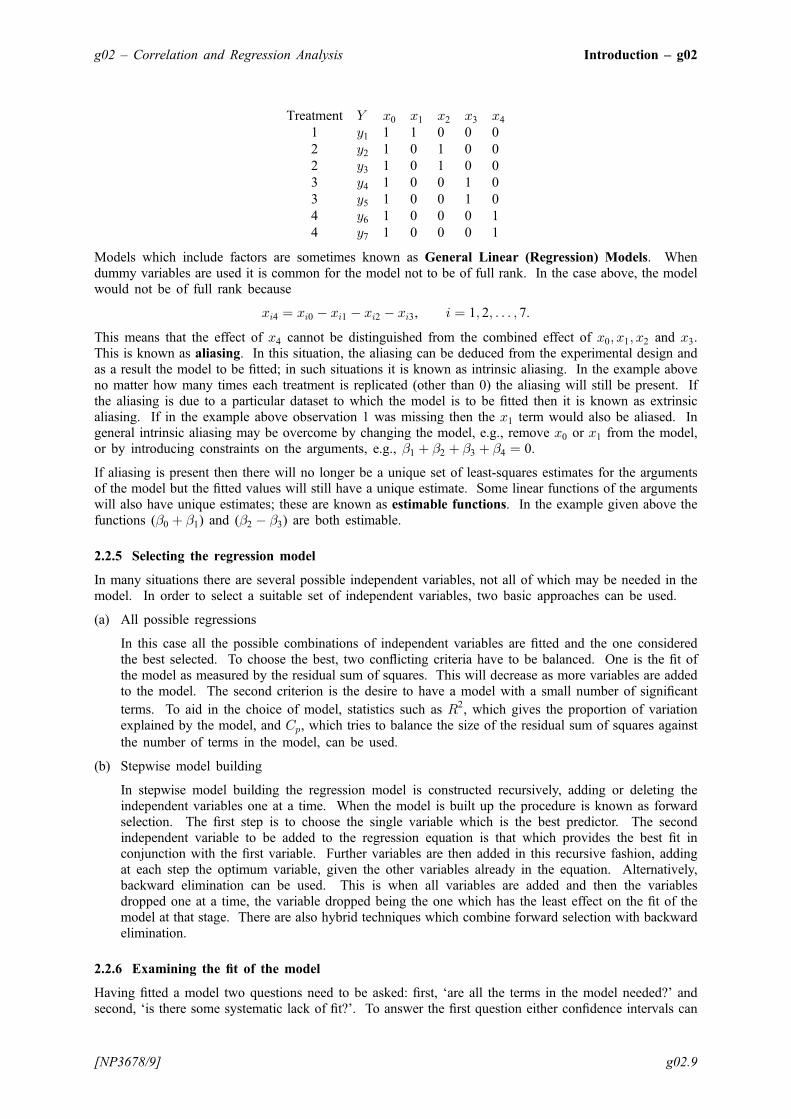
Treatment Y x0 x1 x2 x3 x41 y1 1 1 0 0 02 y2 1 0 1 0 02 y3 1 0 1 0 03 y4 1 0 0 1 03 y5 1 0 0 1 04 y6 1 0 0 0 14 y7 1 0 0 0 1

Models which include factors are sometimes known as General Linear (Regression) Models. Whendummy variables are used it is common for the model not to be of full rank. In the case above, the modelwould not be of full rank because

xi4 ¼ xi0 � xi1 � xi2 � xi3, i ¼ 1; 2; . . . ; 7.

This means that the effect of x4 cannot be distinguished from the combined effect of x0; x1; x2 and x3.This is known as aliasing. In this situation, the aliasing can be deduced from the experimental design andas a result the model to be fitted; in such situations it is known as intrinsic aliasing. In the example aboveno matter how many times each treatment is replicated (other than 0) the aliasing will still be present. Ifthe aliasing is due to a particular dataset to which the model is to be fitted then it is known as extrinsicaliasing. If in the example above observation 1 was missing then the x1 term would also be aliased. Ingeneral intrinsic aliasing may be overcome by changing the model, e.g., remove x0 or x1 from the model,or by introducing constraints on the arguments, e.g., �1 þ �2 þ �3 þ �4 ¼ 0.

If aliasing is present then there will no longer be a unique set of least-squares estimates for the argumentsof the model but the fitted values will still have a unique estimate. Some linear functions of the argumentswill also have unique estimates; these are known as estimable functions. In the example given above thefunctions (�0 þ �1) and (�2 � �3) are both estimable.

2.2.5 Selecting the regression model

In many situations there are several possible independent variables, not all of which may be needed in themodel. In order to select a suitable set of independent variables, two basic approaches can be used.

(a) All possible regressions

In this case all the possible combinations of independent variables are fitted and the one consideredthe best selected. To choose the best, two conflicting criteria have to be balanced. One is the fit ofthe model as measured by the residual sum of squares. This will decrease as more variables are addedto the model. The second criterion is the desire to have a model with a small number of significant

terms. To aid in the choice of model, statistics such as R2, which gives the proportion of variationexplained by the model, and Cp, which tries to balance the size of the residual sum of squares againstthe number of terms in the model, can be used.

(b) Stepwise model building

In stepwise model building the regression model is constructed recursively, adding or deleting theindependent variables one at a time. When the model is built up the procedure is known as forwardselection. The first step is to choose the single variable which is the best predictor. The secondindependent variable to be added to the regression equation is that which provides the best fit inconjunction with the first variable. Further variables are then added in this recursive fashion, addingat each step the optimum variable, given the other variables already in the equation. Alternatively,backward elimination can be used. This is when all variables are added and then the variablesdropped one at a time, the variable dropped being the one which has the least effect on the fit of themodel at that stage. There are also hybrid techniques which combine forward selection with backwardelimination.

2.2.6 Examining the fit of the model

Having fitted a model two questions need to be asked: first, ‘are all the terms in the model needed?’ andsecond, ‘is there some systematic lack of fit?’. To answer the first question either confidence intervals can


[NP3678/9] g02.9

be computed for the arguments or t-tests can be calculated to test hypotheses about the regressionarguments – for example, whether the value of the argument, �k, is significantly different from a specified

value, bk (often zero). If the estimate of �k is �k and its standard error is se �k

� �then the t-statistic is

�k � bkffiffiffiffiffiffiffiffiffiffiffiffiffiffiffise �k

� �r .

It should be noted that both the tests and the confidence intervals may not be independent. AlternativelyF -tests based on the residual sums of squares for different models can also be used to test the significanceof terms in the model. If model 1, giving residual sum of squares RSS1 with degrees of freedom �1, is asub-model of model 2, giving residual sum of squares RSS2 with degrees of freedom �2, i.e., all terms inmodel 1 are also in model 2, then to test if the extra terms in model 2 are needed the F -statistic

F ¼ RSS1 � RSS2ð Þ= �1 � �2ð ÞRSS2=�2

may be used. These tests and confidence intervals require the additional assumption that the errors, ei, areNormally distributed.

To check for systematic lack of fit the residuals, ri ¼ yi � yi, where yi is the fitted value, should beexamined. If the model is correct then they should be random with no discernible pattern. Due to the waythey are calculated the residuals do not have constant variance. Now the vector of fitted values can bewritten as a linear combination of the vector of observations of the dependent variable, y, y ¼ Hy. The

variance-covariance matrix of the residuals is then I �Hð Þ�2, I being the identity matrix. The diagonalelements of H, hii, can therefore be used to standardize the residuals. The hii are a measure of the effectof the ith observation on the fitted model and are sometimes known as leverages.

If the observations were taken serially the residuals may also be used to test the assumption of theindependence of the ei and hence the independence of the observations.

2.2.7 Computational methods

Let X be the n by p matrix of independent variables and y be the vector of values for the dependent

variable. To find the least-squares estimates of the vector of arguments, �, the QR decomposition of X isfound, i.e.,

X ¼ QR�

where R� ¼ R0

� , R being a p by p upper triangular matrix, and Q an n by n orthogonal matrix. If R is

of full rank then � is the solution to

R� ¼ c1

where c ¼ QTy and c1 is the first p rows of c. If R is not of full rank, a solution is obtained by means of asingular value decomposition (SVD) of R,

R ¼ Q�D 00 0

� PT,

where D is a k by k diagonal matrix with nonzero diagonal elements, k being the rank of R, and Q� andP are p by p orthogonal matrices. This gives the solution

� ¼ P1D�1QT

�1c1,

P1 being the first k columns of P and Q�1 being the first k columns of Q�.

This will be only one of the possible solutions. Other estimates may be obtained by applying constraintsto the arguments. If weighted regression with a vector of weights w is required then both X and y are

premultiplied by w1=2.


g02.10 [NP3678/9]

The method described above will, in general, be more accurate than methods based on forming (XTX), (ora scaled version), and then solving the equations

XTX� �

� ¼ XTy.

2.2.8 Robust estimation

Least-squares regression can be greatly affected by a small number of unusual, atypical, or extremeobservations. To protect against such occurrences, robust regression methods have been developed. Thesemethods aim to give less weight to an observation which seems to be out of line with the rest of the datagiven the model under consideration. That is to seek to bound the influence. For a discussion of influencein regression, see Hampel et al. (1986) and Huber (1981).

There are two ways in which an observation for a regression model can be considered atypical. The valuesof the independent variables for the observation may be atypical or the residual from the model may belarge.

The first problem of atypical values of the independent variables can be tackled by calculating weights foreach observation which reflect how atypical it is, i.e., a strongly atypical observation would have a lowweight. There are several ways of finding suitable weights; some are discussed in Hampel et al. (1986).

The second problem is tackled by bounding the contribution of the individual ei to the criterion to beminimized. When minimizing (7) a set of linear equations is formed, the solution of which gives the least-squares estimates. The equations areXn

i¼1

eixij ¼ 0 j ¼ 0; 1; . . . ; k.

These equations are replaced by Xni¼1

ei=�ð Þxij ¼ 0 j ¼ 0; 1; . . . ; k, ð8Þ

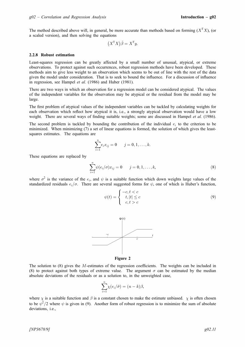
where �2 is the variance of the ei, and is a suitable function which down weights large values of thestandardized residuals ei=�. There are several suggested forms for , one of which is Huber’s function,

tð Þ ¼�c; t < ct; tj j � cc; t > c

8<: ð9Þ

-c

ct

ψ (t)

Figure 2

The solution to (8) gives the M-estimates of the regression coefficients. The weights can be included in(8) to protect against both types of extreme value. The argument � can be estimated by the medianabsolute deviations of the residuals or as a solution to, in the unweighted case,Xn

i¼1

� ei=�ð Þ ¼ n� kð Þ�,

where � is a suitable function and � is a constant chosen to make the estimate unbiased. � is often chosen

to be 2=2 where is given in (9). Another form of robust regression is to minimize the sum of absolutedeviations, i.e.,


[NP3678/9] g02.11

Xni¼1

eij j.

For details of robust regression, see Hampel et al. (1986) and Huber (1981).

Robust regressions using least absolute deviations can be computed using functions in Chapter e02.

2.2.9 Generalized linear models

Generalized linear models are an extension of the general linear regression model discussed above. Theyallow a wide range of models to be fitted. These included certain nonlinear regression models, logistic andprobit regression models for binary data, and log-linear models for contingency tables. A generalizedlinear model consists of three basic components:

(a) A suitable distribution for the dependent variable Y . The following distributions are common:

(i) Normal

(ii) binomial

(iii) Poisson

(iv) gamma

In addition to the obvious uses of models with these distributions it should be noted that the Poissondistribution can be used in the analysis of contingency tables while the gamma distribution can beused to model variance components. The effect of the choice of the distribution is to define therelationship between the expected value of Y , E Yð Þ ¼ , and its variance and so a generalized linearmodel with one of the above distributions may be used in a wider context when that relationshipholds.

(b) A linear model ¼P�jxj, is known as a linear predictor.

(c) A link function g �ð Þ between the expected value of Y and the linear predictor, g ð Þ ¼ . Thefollowing link functions are available:

For the binomial distribution �, observing y out of t:

(i) logistic link: ¼ log t�

� �;

(ii) probit link: ¼ ��1 t

� �;

(iii) complementary log-log: ¼ log � log 1� t

� �� .

For the Normal, Poisson, and gamma distributions:

(i) exponent link: ¼ a, for a constant a;

(ii) identity link: ¼ ;

(iii) log link: ¼ log;

(iv) square root link: ¼ ffiffiffi

p;

(v) reciprocal link: ¼ 1.

For each distribution there is a canonical link. For the canonical link there exist sufficient statisticsfor the arguments. The canonical links are:

(i) Normal – identity;

(ii) binomial – logistic;

(iii) Poisson – logarithmic;

(iv) gamma – reciprocal.

For the general linear regression model described above the three components are:


g02.12 [NP3678/9]

(i) Distribution – Normal;

(ii) Linear model –P�jxj;

(iii) Link – identity.

The model is fitted by maximum likelihood; this is equivalent to least-squares in the case of the Normaldistribution. The residual sums of squares used in regression models is generalized to the concept ofdeviance. The deviance is the logarithm of the ratio of the likelihood of the model to the full model inwhich i ¼ yi, where i is the estimated value of i. For the Normal distribution the deviance is the

residual sum of squares. Except for the case of the Normal distribution with the identity link, the �2 andF -tests based on the deviance are only approximate; also the estimates of the arguments will only beapproximately Normally distributed. Thus only approximate z- or t-tests may be performed on theargument values and approximate confidence intervals computed.

The estimates are found by using an iterative weighted least-squares procedure. This is equivalent to theFisher scoring method in which the Hessian matrix used in the Newton–Raphson method is replaced by itsexpected value. In the case of canonical links the Fisher scoring method and the Newton–Raphson methodare identical. Starting values for the iterative procedure are obtained by replacing the i by yi in theappropriate equations.

2.2.10 Linear mixed effects regression

In a standard linear model the independent (or explanatory) variables are assumed to take the same set ofvalues for all units in the population of interest. This type of variable is called fixed. In contrast, anindependent variable that fluctuates over the different units is said to be random. Modelling a variable asfixed allows conclusions to be drawn only about the particular set of values observed. Modelling avariable as random allows the results to be generalised to the different levels that may have been observed.In general, if the effects of the levels of a variable are thought of as being drawn from a probabilitydistribution of such effects then the the variable is random. If the levels are not a sample of possible levelsthen the variable is fixed. In practice many qualitative variables can be considered as having fixed effectsand most blocking, sampling design, control and repeated measures as having random effects.

In a general linear regression model, defined by

y ¼ X� þ �

where y is a vector of n observations on the dependent variable,

X is an n by p design matrix of independent variables,

� is a vector of p unknown parameters,

and � is a vector of n, independent and identically distributed, unknown errors, with �eN 0; �2� �

.

there are p fixed effects (the �) and a single random effect (the error term �).

An extension to the general linear regression model that allows for additional random effects is the linearmixed effects regression model, (sometimes called the variance components model). One parameterisationof a linear mixed effects model is

y ¼ X� þ Z� þ �

where y is a vector of n observations on the dependent variable,

X is an n by p design matrix of fixed independent variables,

� is a vector of p unknown fixed effects,

Z is an n by q design matrix of random independent variables,

� is a vector of length q of unknown random effects,

� is a vector of length n of unknown random errors,


[NP3678/9] g02.13

and � and � are normally distributed with expectation zero and variance / covariance matrix defined by

Var��

� ¼ G 0

0 R

� .

The functions currently available in this chapter are restricted to cases where R ¼ �2RI, I is the n� nidentity matrix and G is a diagonal matrix. Given this restriction the random variables, Z, can besubdivided into g � q groups containing one or variables. The variables in the ith group are identically

distributed with expectation zero and variance �2i . The model therefore contains three sets of unknowns,the fixed effects, �, the random effects, �, and a vector of gþ 1 variance components, , with

¼ �21; �22; . . . ; ; ; �

2g�1; �

2g; �

2R

�. Rather than work directly with and the full likelihood function, is

replaced by � ¼ �21=�2R; �

22=�

2R; . . . ; �

2g�1=�

2R; �

2g=�

2R; 1

�and the profiled likelihood function is used

instead.

The model parameters are estimated using an iterative method based on maximizing either the restricted(profiled) likelihood function or the (profiled) likelihood functions. Fitting the model via restrictedmaximum likelihood involves maximizing the function

�2lR ¼ log Vj jð Þ þ n� pð Þ log r0V �1r� �

þ log X0V �1X�� þ n� pð Þ 1þ log 2�= n� pð Þð Þð Þ þ n� pð Þ.

Whereas fitting the model via maximum likelihood involves maximizing

�2lR ¼ log Vj jð Þ þ n log r0V �1r� �

þ n log 2�=nð Þ þ n.

In both cases

V ¼ ZGZ0 þR, r ¼ y�Xb and b ¼ X0V �1X� ��1

X0V �1y.

Once the final estimates for � have been obtained, the value of �2R is given by

�2R ¼ r0V �1r� �

= n� pð Þ.

Case weights, Wc, can be incorporated into the model by replacing X0X and Z0Z with X0WcX andZ0WcZ respectively, for a diagonal weight matrix Wc.

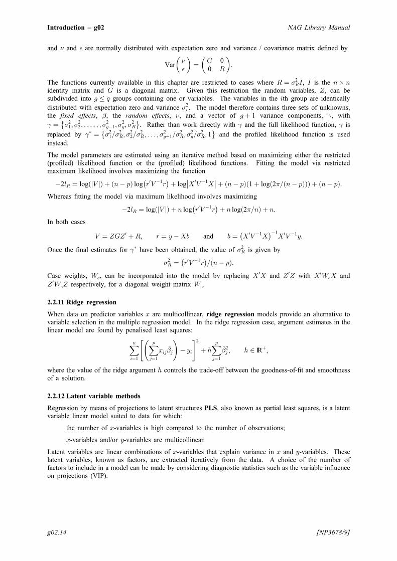
2.2.11 Ridge regression

When data on predictor variables x are multicollinear, ridge regression models provide an alternative tovariable selection in the multiple regression model. In the ridge regression case, argument estimates in thelinear model are found by penalised least squares:

Xni¼1

Xpj¼1

xij�j

!� yi

" #2þ hXpj¼1

�2j , h 2 IRþ,

where the value of the ridge argument h controls the trade-off between the goodness-of-fit and smoothnessof a solution.

2.2.12 Latent variable methods

Regression by means of projections to latent structures PLS, also known as partial least squares, is a latentvariable linear model suited to data for which:

the number of x-variables is high compared to the number of observations;

x-variables and/or y-variables are multicollinear.

Latent variables are linear combinations of x-variables that explain variance in x and y-variables. Theselatent variables, known as factors, are extracted iteratively from the data. A choice of the number offactors to include in a model can be made by considering diagnostic statistics such as the variable influenceon projections (VIP).


g02.14 [NP3678/9]

3 Recommendations on Choice and Use of Available Functions

3.1 Correlation

3.1.1 Product-moment correlation

Let SSx be the sum of squares of deviations from the mean, �x, for the variable x for a sample of size n,i.e.,

SSx ¼Xni¼1

xi � �xð Þ2

and let SCxy be the cross-products of deviations from the means, �x and �y, for the variables x and y for asample of size n, i.e.,

SCxy ¼Xni¼1

xi � �xð Þ yi � �yð Þ.

Then the sample covariance of x and y is

cov x; yð Þ ¼SCxy

n� 1ð Þand the product-moment correlation coefficient is

r ¼ cov x; yð Þffiffiffiffiffiffiffiffiffiffiffiffiffiffiffiffiffiffiffiffiffiffiffiffiffiffiffiffivar xð Þ var yð Þ

p ¼SCxyffiffiffiffiffiffiffiffiffiffiffiffiffiffiffiSSxSSy

q .

nag_sum_sqs (g02buc) computes the sample sums of squares and cross-products deviations from themeans (optionally weighted).

nag_sum_sqs_update (g02btc) updates the sample sums of squares and cross-products and deviations fromthe means by the addition/deletion of a (weighted) observation.

nag_cov_to_corr (g02bwc) computes the product-moment correlation coefficients from the sample sums ofsquares and cross-products of deviations from the means.

The three functions compute only the upper triangle of the correlation matrix which is stored in a one-dimensional array in packed form.

nag_corr_cov (g02bxc) computes both the (optionally weighted) covariance matrix and the (optionallyweighted) correlation matrix. These are returned in two-dimensional arrays. (Note thatnag_sum_sqs_update (g02btc) and nag_sum_sqs (g02buc) can be used to compute the sums of squaresfrom zero.)

3.1.2 Product-moment correlation with missing values

If there are missing values then nag_sum_sqs (g02buc) and nag_corr_cov (g02bxc), as described above,will allow casewise deletion by you giving the observation zero weight (compared with unit weight for anotherwise unweighted computation).

3.1.3 Nonparametric correlation

nag_ken_spe_corr_coeff (g02brc) computes Kendall and/or Spearman nonparametric rank correlationcoefficients. The function allows for a subset of variables to be selected and for observations to beexcluded from the calculations if, for example, they contain missing values.

3.1.4 Partial correlation

nag_partial_corr (g02byc) computes a matrix of partial correlation coefficients from the correlationcoefficients or variance-covariance matrix returned by nag_corr_cov (g02bxc).


[NP3678/9] g02.15

3.1.5 Robust correlation

nag_robust_m_corr_user_fn (g02hlc) and nag_robust_m_corr_user_fn_no_derr (g02hmc) compute robustestimates of the variance-covariance matrix by solving the equations

1

n

Xni¼1

w zik k2� �

zi ¼ 0

and

1

n

Xni¼1

u zik k2� �

zizTi � v zik k2

� �I ¼ 0,

as described in Section 2.1.4 for user-supplied functions w and u. Two options are available for v, eitherv tð Þ ¼ 1 for all t or v tð Þ ¼ u tð Þ.nag_robust_m_corr_user_fn_no_derr (g02hmc) requires only the function w and u to be supplied whilenag_robust_m_corr_user_fn (g02hlc) also requires their derivatives.

In general nag_robust_m_corr_user_fn (g02hlc) will be considerably faster thannag_robust_m_corr_user_fn_no_derr (g02hmc) and should be used if derivatives are available.

nag_robust_corr_estim (g02hkc) computes a robust variance-covariance matrix for the following functions:

u tð Þ ¼ au=t2 if t < a2u

u tð Þ ¼ 1 if a2u � t � b2uu tð Þ ¼ bu=t

2 if t > b2u

and

w tð Þ ¼ 1 if t � cww tð Þ ¼ cw=t if t > cw

for constants au, bu and cw.

These functions solve a minimax space problem considered by Huber (1981). The values of au, bu and cware calculated from the fraction of gross errors; see Hampel et al. (1986) and Huber (1981).

To compute a correlation matrix from the variance-covariance matrix nag_cov_to_corr (g02bwc) may beused.

3.1.6 Nearest correlation matrix

nag_nearest_correlation (g02aac) calculates the nearest correlation matrix to a real, square matrix.

3.2 Regression

3.2.1 Simple linear regression

Two functions are provided for simple linear regression. The function nag_simple_linear_regression(g02cac) calculates the argument estimates for a simple linear regression with or without a constant term.The function nag_regress_confid_interval (g02cbc) calculates fitted values, residuals and confidenceintervals for both the fitted line and individual observations. This function produces the informationrequired for various regression plots.

3.2.2 Multiple linear regression – general linear model

nag_regsn_mult_linear (g02dac) fits a general linear regression model using the QR method and an SVD ifthe model is not of full rank. The results returned include: residual sum of squares, argument estimates,their standard errors and variance-covariance matrix, residuals and leverages. There are also severalfunctions to modify the model fitted by nag_regsn_mult_linear (g02dac) and to aid in the interpretation ofthe model.

nag_regsn_mult_linear_addrem_obs (g02dcc) adds or deletes an observation from the model.


g02.16 [NP3678/9]

nag_regsn_mult_linear_upd_model (g02ddc) computes the argument estimates, and their standard errorsand variance-covariance matrix for a model that is modified by nag_regsn_mult_linear_addrem_obs(g02dcc), nag_regsn_mult_linear_add_var (g02dec) or nag_regsn_mult_linear_delete_var (g02dfc).

nag_regsn_mult_linear_add_var (g02dec) adds a new variable to a model.

nag_regsn_mult_linear_delete_var (g02dfc) drops a variable from a model.

nag_regsn_mult_linear_newyvar (g02dgc) fits the regression to a new dependent variable, i.e., keeping thesame independent variables.

nag_regsn_mult_linear_tran_model (g02dkc) calculates the estimates of the arguments for a given set ofconstraints, (e.g., arguments for the levels of a factor sum to zero) for a model which is not of full rankand the SVD has been used.

nag_regsn_mult_linear_est_func (g02dnc) calculates the estimate of an estimable function and its standarderror.

Note: nag_regsn_mult_linear_add_var (g02dec) also allows you to initialize a model building process andthen to build up the model by adding variables one at a time.

3.2.3 Selecting regression models

To aid the selection of a regression model the following functions are available.

nag_all_regsn (g02eac) computes the residual sums of squares for all possible regressions for agiven set of dependent variables. The function allows some variables to be forced into allregressions.

nag_cp_stat (g02ecc) computes the values of R2 and Cp from the residual sums of squares asprovided by nag_all_regsn (g02eac).

nag_step_regsn (g02eec) enables you to fit a model by forward selection. You may callnag_step_regsn (g02eec) a number of times. At each call the function will calculate the changes inthe residual sum of squares from adding each of the variables not already included in the model,select the variable which gives the largest change and then if the change in residual sum of squaresmeets the given criterion will add it to the model.

nag_full_step_regsn (g02efc) uses a full stepwise selection to choose a subset of the explanatoryvariables. The method repeatedly applies a forward selection step followed by a backwardelimination step until neither step updates the current model.

3.2.4 Residuals

nag_regsn_std_resid_influence (g02fac) computes the following standardized residuals and measures ofinfluence for the residuals and leverages produced by nag_regsn_mult_linear (g02dac):

(i) Internally studentized residual;

(ii) Externally studentized residual;

(iii) Cook’s D statistic;

(iv) Atkinson’s T statistic.

nag_durbin_watson_stat (g02fcc) computes the Durbin–Watson test statistic and bounds for its significanceto test for serial correlation in the errors, ei.

3.2.5 Robust regression

For robust regression using M-estimates instead of least-squares the function nag_robust_m_regsn_estim(g02hac) will generally be suitable. nag_robust_m_regsn_estim (g02hac) provides a choice of four -functions (Huber’s, Hampel’s, Andrew’s and Tukey’s) plus two different weighting methods and theoption not to use weights. If other weights or different -functions are needed the functionnag_robust_m_regsn_user_fn (g02hdc) may be used. nag_robust_m_regsn_user_fn (g02hdc) requiresyou to supply weights, if required, and also functions to calculate the -function and, optionally, the�-function. nag_robust_m_regsn_wts (g02hbc) can be used in calculating suitable weights. The function


[NP3678/9] g02.17

nag_robust_m_regsn_param_var (g02hfc) can be used after a call to nag_robust_m_regsn_user_fn(g02hdc) in order to calculate the variance-covariance estimate of the estimated regression coefficients.

For robust regression, using least absolute deviation, nag_lone_fit (e02gac) can be used.

3.2.6 Generalized linear models

There are four functions for fitting generalized linear models. The output includes: the deviance, argumentestimates and their standard errors, fitted values, residuals and leverages. The functions are:

nag_glm_normal (g02gac) Normal distribution;

nag_glm_binomial (g02gbc) binomial distribution;

nag_glm_poisson (g02gcc) Poisson distribution;

nag_glm_gamma (g02gdc) gamma distribution.

While nag_glm_normal (g02gac) can be used to fit linear regression models (i.e., by using an identity link)this is not recommended as nag_regsn_mult_linear (g02dac) will fit these models more efficiently.nag_glm_poisson (g02gcc) can be used to fit log-linear models to contingency tables.

In addition to the functions to fit the models there is one function to predict from the fitted model and twofunctions to aid interpretation when the fitted model is not of full rank, i.e., aliasing is present.

nag_glm_predict (g02gpc) computes a predicted value and its associated standard error based on apreviously fitted generalized linear model.

nag_glm_tran_model (g02gkc) computes argument estimates for a set of constraints, (e.g., sum ofeffects for a factor is zero), from the SVD solution provided by the fitting function.

nag_glm_est_func (g02gnc) calculates an estimate of an estimable function along with its standarderror.

3.2.7 Linear mixed effects regression

There are two functions for fitting linear mixed effects regression. The functions are:

nag_reml_mixed_regsn (g02jac) uses restricted maximum likelihood (REML) to fit the model.

nag_ml_mixed_regsn (g02jbc) uses maximum likelihood to fit the model.

for both functions the output includes: either the maximum likelihood or restricted maximum likelihoodand the fixed and random argument estimates, along with their standard errors.

As the estimates of the variance components are found using an iterative procedure initial values must besupplied for each �. In both functions you can either specify these initial values, or allow the function tocalculate them from the data using minimum variance quadratic unbiased estimation (MIVQUE0). Settingthe maximum number of iterations to zero in either function will return the corresponding likelihood,argument estimates and standard errors based on these initial values.

3.2.8 Ridge regression

nag_regsn_ridge_opt (g02kac) calculates a ridge regression, optimizing the ridge argument according toone of four prediction error criteria.

nag_regsn_ridge (g02kbc) calculates ridge regressions for a given set of ridge arguments.

3.2.9 Partial Least-squares (PLS)

nag_pls_orth_scores_svd (g02lac) calculates a nonlinear, iterative PLS by using singular valuedecomposition.

nag_pls_orth_scores_wold (g02lbc) calculates a nonlinear, iterative PLS by using Wold’s method.

nag_pls_orth_scores_fit (g02lcc) calculates argument estimates for a given number of PLS factors.

nag_pls_orth_scores_pred (g02ldc) calculates predictions given a PLS model.


g02.18 [NP3678/9]

3.2.10 Polynomial regression and nonlinear regression

No functions are currently provided in this chapter for polynomial regression. If you wish to performpolynomial regressions you have three alternatives: you can use the multiple linear regression functions,nag_regsn_mult_linear (g02dac), with a set of independent variables which are in fact simply the samesingle variable raised to different powers, or you can use the function nag_dummy_vars (g04eac) tocompute orthogonal polynomials which can then be used with nag_regsn_mult_linear (g02dac), or you canuse the functions in Chapter e02 (Curve and Surface Fitting) which fit polynomials to sets of data pointsusing the techniques of orthogonal polynomials. This latter course is to be preferred, since it is moreefficient and liable to be more accurate, but in some cases more statistical information may be requiredthan is provided by those functions, and it may be necessary to use the functions of this chapter.

More general nonlinear regression models may be fitted using the optimization functions in Chapter e04,which contains functions to minimize the functionXn

i¼1

e2i

where the regression arguments are the variables of the minimization problem.

4 Index

Computes the nearest correlation matrix using the method of Qi and Sun.......... nag_nearest_correlation (g02aac)

Generalized linear models:binomial errors ............................................................................................. nag_glm_binomial (g02gbc)computes estimable function ....................................................................... nag_glm_est_func (g02gnc)gamma errors ................................................................................................. nag_glm_gamma (g02gdc)Normal errors .................................................................................................. nag_glm_normal (g02gac)Poisson errors ................................................................................................ nag_glm_poisson (g02gcc)transform model parameters .................................................................... nag_glm_tran_model (g02gkc)

Hierarchical mixed effects regression:initiation ..................................................................................................... nag_hier_mixed_init (g02jcc)using maximum likelihood .............................................................. nag_ml_hier_mixed_regsn (g02jec)using restricted maximum likelihood ........................................... nag_reml_hier_mixed_regsn (g02jdc)

Linear mixed effects regression:via maximum likelihood (ML) ................................................................ nag_ml_mixed_regsn (g02jbc)via restricted maximum likelihood (REML) ........................................ nag_reml_mixed_regsn (g02jac)

Multiple linear regression/General linear model:add/delete observation from model ................................. nag_regsn_mult_linear_addrem_obs (g02dcc)add independent variable to model ....................................... nag_regsn_mult_linear_add_var (g02dec)computes estimable function ................................................. nag_regsn_mult_linear_est_func (g02dnc)delete independent variable from model ............................ nag_regsn_mult_linear_delete_var (g02dfc)general linear regression model ............................................................ nag_regsn_mult_linear (g02dac)regression for new dependent variable ................................ nag_regsn_mult_linear_newyvar (g02dgc)regression parameters from updated model ..................... nag_regsn_mult_linear_upd_model (g02ddc)transform model parameters ............................................. nag_regsn_mult_linear_tran_model (g02dkc)

Non-parametric rank correlation (Kendall and/or Spearman):missing values

casewise treatment of missing valuespreserving input data ............................................................... nag_ken_spe_corr_coeff (g02brc)

Partial least-squares:calculates predictions given an estimated PLS model .................... nag_pls_orth_scores_pred (g02ldc)fits a PLS model for a given number of factors ................................ nag_pls_orth_scores_fit (g02lcc)


[NP3678/9] g02.19

orthogonal scores using SVD ............................................................ nag_pls_orth_scores_svd (g02lac)orthogonal scores using Wold’s method ......................................... nag_pls_orth_scores_wold (g02lbc)

Product-moment correlation:correlation matrix

compute correlation and covariance matrices ............................................... nag_corr_cov (g02bxc)compute from sum of squares matrix ..................................................... nag_cov_to_corr (g02bwc)compute partial correlation and covariance matrices ............................... nag_partial_corr (g02byc)

sum of squares matrixcompute ........................................................................................................... nag_sum_sqs (g02buc)update .................................................................................................. nag_sum_sqs_update (g02btc)

Residuals:Durbin–Watson test ............................................................................. nag_durbin_watson_stat (g02fcc)standardized residuals and influence statistics ......................... nag_regsn_std_resid_influence (g02fac)

Ridge regression:ridge parameter(s) supplied ............................................................................ nag_regsn_ridge (g02kbc)ridge parameter optimized ....................................................................... nag_regsn_ridge_opt (g02kac)

Robust correlation:Huber’s method ..................................................................................... nag_robust_corr_estim (g02hkc)user-supplied weight function only .............................. nag_robust_m_corr_user_fn_no_derr (g02hmc)user-supplied weight function plus derivatives ............................ nag_robust_m_corr_user_fn (g02hlc)

Robust regression:compute weights for use with nag_robust_m_regsn_user_fn (g02hdc)

.......... nag_robust_m_regsn_wts (g02hbc)standard M-estimates ..................................................................... nag_robust_m_regsn_estim (g02hac)user supplies weight functions .................................................. nag_robust_m_regsn_user_fn (g02hdc)variance-covariance matrix following nag_robust_m_regsn_user_fn (g02hdc)

.......... nag_robust_m_regsn_param_var (g02hfc)

Selecting regression model:all possible regressions ........................................................................................ nag_all_regsn (g02eac)forward selection ............................................................................................... nag_step_regsn (g02eec)

R2 and Cp statistics ................................................................................................ nag_cp_stat (g02ecc)

Simple linear regression:no intercept ................................................................................... nag_regress_confid_interval (g02cbc)with intercept .............................................................................. nag_simple_linear_regression (g02cac)

Stepwise linear regression:Clarke’s sweep algorithm ........................................................................... nag_full_step_regsn (g02efc)

5 Functions Withdrawn or Scheduled for Withdrawal

None.

6 References

Atkinson A C (1986) Plots, Transformations and Regressions Clarendon Press, Oxford

Churchman C W and Ratoosh P (1959) Measurement Definitions and Theory Wiley

Cook R D and Weisberg S (1982) Residuals and Influence in Regression Chapman and Hall

Draper N R and Smith H (1985) Applied Regression Analysis (2nd Edition) Wiley


g02.20 [NP3678/9]

Hammarling S (1985) The singular value decomposition in multivariate statistics SIGNUM Newsl. 20 (3)2–25

Hampel F R, Ronchetti E M, Rousseeuw P J and Stahel W A (1986) Robust Statistics. The ApproachBased on Influence Functions Wiley

Hays W L (1970) Statistics Holt, Rinehart and Winston

Huber P J (1981) Robust Statistics Wiley

Kendall M G and Stuart A (1973) The Advanced Theory of Statistics (Volume 2) (3rd Edition) Griffin

McCullagh P and Nelder J A (1983) Generalized Linear Models Chapman and Hall

Searle S R (1971) Linear Models Wiley

Siegel S (1956) Non-parametric Statistics for the Behavioral Sciences McGraw–Hill

Weisberg S (1985) Applied Linear Regression Wiley___________________________________________________________________________________________________________________________________________________________________________________________________________________________________________________________________________________________________________________________________________________________________________________________________________________________________________________________________


[NP3678/9] g02.21 (last)

nag library chapter introduction g02 – correlation … · nag library chapter introduction g02...

Documents