myrick, kenneth b. coastal bathymetry using satellite

This document was downloaded on May 04, 2015 at 23:14:28

Author(s) Myrick, Kenneth B.

Title Coastal bathymetry using satellite observation in support of intelligence preparation ofthe environment

Publisher Monterey, California. Naval Postgraduate School

Issue Date 2011-09

URL http://hdl.handle.net/10945/5519

NAVAL

POSTGRADUATE SCHOOL

MONTEREY, CALIFORNIA

THESIS

Approved for public release; distribution is unlimited

COASTAL BATHYMETRY USING SATELLITE OBSERVATION IN SUPPORT OF INTELLIGENCE

PREPARATION OF THE ENVIRONMENT

by

Kenneth B. Myrick II

September 2011

Thesis Advisor: Richard C. Olsen Second Reader: Jamie MacMahan

THIS PAGE INTENTIONALLY LEFT BLANK

i

REPORT DOCUMENTATION PAGE Form Approved OMB No. 0704-0188 Public reporting burden for this collection of information is estimated to average 1 hour per response, including the time for reviewing instruction, searching existing data sources, gathering and maintaining the data needed, and completing and reviewing the collection of information. Send comments regarding this burden estimate or any other aspect of this collection of information, including suggestions for reducing this burden, to Washington headquarters Services, Directorate for Information Operations and Reports, 1215 Jefferson Davis Highway, Suite 1204, Arlington, VA 22202-4302, and to the Office of Management and Budget, Paperwork Reduction Project (0704-0188), Washington, DC 20503. 1. AGENCY USE ONLY (Leave blank)

2. REPORT DATE September 2011

3. REPORT TYPE AND DATES COVERED Master’s Thesis

4. TITLE AND SUBTITLE Coastal Bathymetry Using Satellite Observation in Support of Intelligence Preparation of the Environment

5. FUNDING NUMBERS

6. AUTHOR(S) Kenneth B. Myrick II 7. PERFORMING ORGANIZATION NAME(S) AND ADDRESS(ES)

Naval Postgraduate School Monterey, CA 93943-5000

8. PERFORMING ORGANIZATION REPORT NUMBER

9. SPONSORING /MONITORING AGENCY NAME(S) AND ADDRESS(ES) N/A

10. SPONSORING/MONITORING AGENCY REPORT NUMBER

11. SUPPLEMENTARY NOTES The views expressed in this thesis are those of the author and do not reflect the official policy or position of the Department of Defense or the U.S. Government. IRB Protocol number NA.

12a. DISTRIBUTION / AVAILABILITY STATEMENT Approved for public release; distribution is unlimited

12b. DISTRIBUTION CODE

13. ABSTRACT (maximum 200 words) Subaqueous beach profiles are obtained for littoral regions near Camp Pendleton, CA, using observations of wave motion. Imagery was acquired from WorldView2 Satellite on 24 March 2010. Two sequential images taken 10 seconds apart are used for the analyses herein. Water depths were calculated using linear dispersion relationship for surface gravity waves. Depth profiles were established from shoreline out to 1 kilometer offshore and depths of up to 15 meters. Comparisons with USGS DEM values show agreement within five percent in the surf zone (shoreline to wave breaking) and one percent outside the surf zone (offshore of wave breaking). 14. SUBJECT TERMS Remote Sensing, Multispectral, 8-Color, Bathymetry, World View-2, ENVI, Principal Component Transform, Depth Inversion, Wave Methods, Dispersion Relation, IPE, Intelligence Preparation of the Environment.

15. NUMBER OF PAGES

75 16. PRICE CODE

17. SECURITY CLASSIFICATION OF REPORT

Unclassified

18. SECURITY CLASSIFICATION OF THIS PAGE

Unclassified

19. SECURITY CLASSIFICATION OF ABSTRACT

Unclassified

20. LIMITATION OF ABSTRACT

UU NSN 7540-01-280-5500 Standard Form 298 (Rev. 2-89) Prescribed by ANSI Std. 239-18

ii


iii

Approved for public release; distribution is unlimited

COASTAL BATHYMETRY USING SATELLITE OBSERVATION IN SUPPORT OF INTELLIGENCE PREPARATION OF THE ENVIRONMENT

Kenneth B. Myrick II Lieutenant Commander, United States Navy B.S., Thomas A. Edison State College, 2000

Submitted in partial fulfillment of the requirements for the degree of

MASTER OF SCIENCE IN SPACE SYSTEMS OPERATIONS

from the

NAVAL POSTGRADUATE SCHOOL September 2011

Author: Kenneth B. Myrick II

Approved by: Dr. Richard C. Olsen Thesis Advisor

Dr. Jamie MacMahan Second Reader

Dr. Rudy Panholzer Chair, Space Systems Academic Group

iv


v

ABSTRACT

Subaqueous beach profiles are obtained for littoral regions near Camp Pendleton, CA,

using observations of wave motion. Imagery was acquired from WorldView2 Satellite

on 24 March 2010. Two sequential images taken 10 seconds apart are used for the

analyses herein. Water depths were calculated using linear dispersion relationship for

surface gravity waves. Depth profiles were established from shoreline out to 1 kilometer

offshore and depths of up to 15 meters. Comparisons with USGS DEM values show

agreement within five percent in the surf zone (shoreline to wave breaking) and

one percent outside the surf zone (offshore of wave breaking).

vi


vii

TABLE OF CONTENTS

I. INTRODUCTION........................................................................................................1 A. PURPOSE OF RESEARCH ...........................................................................1 B. SPECIFIC OBJECTIVES...............................................................................2

II. BACKGROUND ..........................................................................................................3 A. HISTORY .........................................................................................................3

1. Early Bathymetry of Denied Areas in Support of Military Operations ............................................................................................3 a. The Waterline Method ..............................................................3 b. The Transparency Method........................................................4 c. The Wave Celerity Method .......................................................5 d. The Wave Period Method .........................................................6

2. Operational Capability to Determine Nearshore Bathymetry ........8 a. Sunglint .....................................................................................8 b. Scale ...........................................................................................9 c. Bottom Slope Conditions ........................................................10

3. Modern Studies to Determine Nearshore Bathymetry ...................10 a. X-Band Marine Radar ............................................................10 b. Video Imagery and Wave number ..........................................13 c. Satellite Imagery .....................................................................15 d. Neuro-Fuzzy Technique .........................................................16

B. THEORY ........................................................................................................17 1. Periodic Waves ...................................................................................17 2. Linear Airy-Wave ..............................................................................19 3. Cnoidal and Solitary Wave ...............................................................23

III. PROBLEM .................................................................................................................25 A. DEFINITION .................................................................................................25 B. MATERIALS .................................................................................................25

1. WorldView-2 Sensor ..........................................................................25 2. The Environment for Visualizing Images 4.7 (ENVI) ....................28 3. USGS Digital Elevation Model for Southern California ................28

IV. METHODS AND OBSERVATIONS .......................................................................31 A. WORLDVIEW-2 IMAGERY OF CAMP PENDLETON .........................31

1. Collection ............................................................................................31 2. Image Processing ................................................................................34

a. Image Registration ..................................................................34 b. Image Rotation and Resizing ..................................................35

3. Principal Component Transforms....................................................36 B. SURF ZONE ...................................................................................................37 C. OUTSIDE OF THE SURF ZONE ................................................................38

V. ANALYSIS .................................................................................................................41

viii

A. SURF ZONE ...................................................................................................41 B. OUTSIDE OF THE SURF ZONE ................................................................44

VI. SUMMARY ................................................................................................................49

VII. CONCLUSION ..........................................................................................................51

APPENDIX .............................................................................................................................53

LIST OF REFERENCES ......................................................................................................55

INITIAL DISTRIBUTION LIST .........................................................................................57

ix

LIST OF FIGURES

Figure 1. Curves relating water depth to wave length and celerity (From Williams, 1947) ..................................................................................................................5

Figure 2. Curves relating wave period to depth and wave length (From Williams, 1947) ..................................................................................................................7

Figure 3. (a) Optimum wave detection: sun rays perpendicular to wave direction. (b) Poor wave detection: sun rays parallel to wave direction. (From Caruthers et al., 1985) ........................................................................................................9

Figure 4. Plot of wave celerity from X-Band marine radar (From Bell, 1999)...............11 Figure 5. Plot of water depth calculated from X-Band radar data (From Bell, 1999) ....12 Figure 6. Plot of water depth calculated from X-Band radar data using 2D analyses

(From Abileah & Trizna, 2010) .......................................................................13 Figure 7. Plot of wave angle and water depth estimates for Duck, NC using video

technique (From Stockdon & Holman, 2000)..................................................14 Figure 8. Bathymetry of San Diego Harbor estimated by IKONOS (left) compared

with Fugro multibeam depth (right) (From Abileah, 2006) .............................15 Figure 9. Plot of estimated depth by ANFIS versus predetermined depth (From

Corucci et al., 2011) .........................................................................................17 Figure 10. General Wave Characteristics (From Komar, 1998) .......................................18 Figure 11. Linear Airy-wave approximations for varying depths (After Komar, 1998) ...21 Figure 12. Comparison of Solitary, Cnoidal, and Airy wave profiles (From Komar,

1998) ................................................................................................................24 Figure 13. WorldView-2 Satellite (From DigitalGlobe) ...................................................26 Figure 14. DigitalGlobe satellite spectral coverage (From DigitalGlobe, 2010) ..............27 Figure 15. USGS location map and identifiers (IDs) for the 45 DEMs (From Barnard

& Hoover, 2010) ..............................................................................................29 Figure 16. STK simulation of WorldView-2 Camp Pendleton area collection (From

McCarthy & Naval Postgraduate School [U.S.], 2010) ...................................31 Figure 17. Physical Structure of Imagery Scenes (From DigitalGlobe) ...........................32 Figure 18. Google Earth representation of WorldView-2 data for Camp Pendleton

area (From McCarthy & Naval Postgraduate School (U.S.), 2010) ................33 Figure 19. Ground reference point location for image to image registration (From

McCarthy & Naval Postgraduate School [U.S.], 2010) ...................................35 Figure 20. Image rotation 131 degrees ..............................................................................35 Figure 21. Resized Image ..................................................................................................36 Figure 22. Original Eight Bands for image P007 ..............................................................37 Figure 23. Eight Principal Component Banks for image P007 .........................................37 Figure 24. Change detection image for surf zone .............................................................38 Figure 25. Image P007 (left) and P009 (right) represented by 765 bands in RGB and

image equalization enhancement .....................................................................39 Figure 26. Calculating wave distance using ENVI measurement tool for surf zone ........41 Figure 27. Ground Truth determination from USGS DEM sd10 for surf zone ................42 Figure 28. Plot of estimated depth versus ground truth depth in the surf zone .................43

x

Figure 29. Calculating wave distance for outside the surf zone ........................................45 Figure 30. Ground Truth determination from USGS DEM for outside the surf zone ......46 Figure 31. Plot of estimated depth versus ground truth depth outside the surf zone ........47

xi

LIST OF TABLES

Table 1. Equations derived from Linear Airy-wave theory (After Komar, 1998) .........22 Table 2. WorldView-2 Specifications (After DigitalGlobe, 2011) ................................27 Table 3. USGS Individual DEM names and locations (From Barnard & Hoover,

2010) ................................................................................................................29 Table 4. Summary of image meta-data information (From McCarthy & Naval

Postgraduate School, 2010) .............................................................................34 Table 5. Data table for depth data points outside of the surf zone .................................53 Table 6. Data table for surf zone depth data points .......................................................54

xii


xiii

LIST OF ACRONYMS AND ABBREVIATIONS

AGI Analytical Graphics Inc.

ANFIS Adaptive-Network-based Fuzzy Inference System

CEOF Complex Empirical Orthogonal Function

CRAB Coastal Research Amphibious Buggy

DEM Digital Elevation Model

ENVI Environment for Visualizing Images

HADR Humanitarian and Disaster Relief

IfSAR Interferometric Synthetic Aperture Radar

IPE Intelligence Preparation of the Environment

LEO Low Earth Orbit

LIDAR Light Detection and Ranging

RST Resampling, Scaling, and Translation

SNR Signal to Noise Ration

SONAR Sound Navigation and Ranging

STK Satellite Tool Kit

UAV Unmanned Aerial Vehicle

USGS United States Geological Survey

xiv


xv

ACKNOWLEDGMENTS

I would like to thank Dr. Richard C. Olsen and Dr. Jamie MacMahan for their

guidance and support during the development of this thesis. Additionally, I would like to

thank Ms. Angela Kim and Ms. Krista Lee for their tremendous support and

encouragement throughout this process. Their encouragement was invaluable and very

much appreciated.

Furthermore, I would like to thank Major Frank Harmon for continually providing

me with the motivation I needed to complete this thesis. I would also like to give a

special thanks to his loving wife Ms. Cariann Colman, for her support, encouragement,

motivation, and providing me with nourishing home-cooked meals in the absence of my

family during the last three months of this process.

Finally, I would like to thank my loving wife, Patsy, and our two boys, Dusty and

Dakota, for their love, support, encouragement, and understanding. They are my life, and

without them none of this would have been possible.

xvi


1

I. INTRODUCTION

A. PURPOSE OF RESEARCH

Nearshore bathymetry is used for Intelligence Preparation of the Environment

(IPE) in support of amphibious operations, Humanitarian and Disaster Relief (HADR),

and mine warfare planning operations. “The Navy, in support of amphibious operations,

also requires the ability to remotely and surreptitiously determine the bathymetry profile

of the ocean near amphibious landing zones” (OPNAV N2/N6, 2010). In most instances,

IPE will be conducted in denied areas where it is not feasible or in many instances

possible for platforms to gain the required access to conduct bathymetry determination

from the standard Navy operational tools such as Light Detection and Ranging (LIDAR)

or Sound Navigation and Ranging (SONAR). Although bathymetry can be measured

through various means, satellites from Low Earth Orbit (LEO) can safely transit over

denied territories to produce nearshore subaqueous beach profiles. The wave celerity

method using the linear dispersion relationship for surface gravity waves is a convenient

method to accurately estimate nearshore subaqueous beach profiles from satellite

imagery.

Estimating water depth from aerial photography by the linear dispersion relation

for surface gravity waves is not a new technique. In fact, a very similar method for

determining the bathymetry off hostile beaches was used during both World War I and

World War II (Caruthers, Arnone, Howard, Haney, & Durham, 1985; Williams, 1947).

However, due to cost and a number of significant limitations affecting the accuracy, once

the stress of war and need to access denied coastal areas was removed the Navy stopped

using it as a peace time tool (Williams, 1947).

The purpose of this thesis is to show that determining nearshore bathymetry from

multispectral satellite imagery is a viable and accurate method in support of IPE. If

shallow water wave celerity or wave length can be determined from satellite imagery,

then water depth can be calculated by the linear dispersion relation for surface gravity

waves. This thesis will show that, by taking advantage of the different characteristics of

2

multispectral imagery, wave crest can be clearly resolved allowing for the determination

of both wave celerities and wave lengths. In addition, a number of the limitations

associated with both methods of the linear dispersion relation for surface gravity waves to

estimate water depth can be minimized resulting in sufficiently detailed and accurate

depth determination for the purpose of IPE in support of amphibious operations, HADR,

and mine warfare planning.

B. SPECIFIC OBJECTIVES

For the purpose of this study, ten WorldView-2 multispectral images were taken

in rapid succession at approximately ten second intervals of Camp Pendleton, California.

The imagery was processed with Environment for Visualizing Images (ENVI) software

to register the images, identify wave crest, measure wave lengths, and determine wave

celerity. Depth was estimated at approximately eighty locations by applying the linear

dispersion relation for surface gravity waves, by the celerity method, to the data derived

from the imagery processing. Next, these estimated depths were compared to ground

truth data as determined from a United States Geological Survey (USGS) Digital

Elevation Model (DEM). Finally, this study demonstrates that applying the linear

dispersion relation for surface gravity waves to wave data, determined from multispectral

satellite electro-optical imagery, is a viable technique for determining bathymetry in

denied or restricted areas in support of IPE.

3

II. BACKGROUND

A. HISTORY

1. Early Bathymetry of Denied Areas in Support of Military Operations

There are examples where the U.S. military has relied heavily on bathymetry

determination of denied or hostile areas by remote sensing methods to ensure the success

of military operations as far back as World War I. The coastal bathymetry off both the

Beaches of Normandy and the beaches on the Flanders coast were determined with early

remote sensing methods to ensure the success of those operations (Williams, 1947).

During a time of hostilities leading up to these military operations it was not practical to

conduct hydrographic surveys off the coast of these enemy held beaches. However, there

were very important questions that needed to be answered to ensure the success of the

operations and the accurate determination of coastal bathymetry held the answers to

many of those questions. The importance of determining coastal bathymetry to answer

questions like: “How far to seaward will craft ground? To what extent will it be necessary

to waterproof the vehicles to be unloaded? What kind of craft should be used? Will

special equipment such as pontoons be needed? Will men be in danger of drowning in

deeper water inshore of where the craft ground?” (Williams, 1947) and determination of

beach obstacles is obvious when landing forces on hostile beaches, and these same

questions are still applicable today. In 1947, W.W. Williams outlined four ways to

determine coastal bathymetry with remote sensing.

a. The Waterline Method

The Waterline Method was the method used for both Flanders and

Normandy. In this method, bathymetry determination is made by drawing contours of

the waterlines on aerial photographs taken of shorelines at carefully recorded times and

then computing the tide height from the time record from the Admiralty Tables. This

method was used throughout World War II for almost every amphibious operation due to

its simplicity and ease to be operationalized (Williams, 1947).

4

This method has a number of significant limitations; however, the worst of

which was the fact that it was useless for bathymetry below the low spring tide levels and

had no application to tideless waters. Therefore, it was determined that some other

method of obtaining coastal bathymetry was needed in order to calculate bathymetry out

to at least two fathoms below mean low water-level (Williams, 1947).

b. The Transparency Method

In 1942, it was noted that in a photograph of a swimming pool the image

density was greater in the deeper end than in the shallow end. Further investigation

showed that photographs of beaches revealed the same phenomenon in the coastal waters

but not always (Williams, 1947). The transparency method is based on the fact that light

on the surface of the water is reflected, absorbed, transmitted, and scattered by varying

amounts (Olsen, 2007). The light that is transmitted is reflected off of light colored

sediments and is transmitted up through the water and toward the imaging sensor, in

shallow water.

In 1943, this method was used to map the deep water channel in the Seine

River below Rouen and was used qualitatively to locate sandbanks and shoals. However,

this method suffers from numerous limitations that made it impractical to operationalize

primarily due to the fact that “it is doubtful whether quantitatively the method can be of

great value” (Williams, 1947). This is due to limitations, such as choppy seas, which

increase scattering, resulting in the image coming from the water surface and not the

seabed. Other serious limitations are suspension of particulates in the water that prevent

light from transmitting through the entire water column, and dark plant and sediment

materials on the seabed that increase absorption and decrease reflection of incident light.

Both result in density of the photographic image not being a simple function of water

depth. These serious limitations resulted in this method being determined as unreliable

and dangerous for military operations and therefore was abandoned (Williams, 1947).

This approach has since been revisited in several modern studies using modern

technology and multispectral imagery, and is proving to be a practical method (Gao,

2009).

5

c. The Wave Celerity Method

The wave celerity method relies on the linear dispersion relationship

between wave celerity, wave period, wave length, and water depth. The wave celerity

and wave length are determined from successive images where the exact time between

images and image scale are known. Figure 1 shows curves used to quickly determine

water depth once wave length and wave celerity were known (Williams, 1947).

Figure 1. Curves relating water depth to wave length and celerity (From Williams, 1947)

The curves in Figure 1 show that waves with long wave lengths travel at

faster speeds than those with shorter wave lengths. In addition, in deep water a wave’s

celerity is unaffected by depth, but as waves enter shallow water at depths less than their

wave length they begin to feel the affect of the bottom. This results in a decrease in wave

6

celerity corresponding to the decrease in depth. This relation allows the expression of

depth as a function of wave celerity, which will be discussed in more detail in Section B

of this chapter (Williams, 1947).

In 1947, Williams noted that this method suffered from a number of issues

to include accuracy of image acquisition times, scale and registration of images, and low

image resolution (Williams, 1947). This method is very similar to the method explored

in this thesis as the same math is valid, however, with the use of multispectral satellite

imagery much of the afore mentioned uncertainties can easily be overcome.

d. The Wave Period Method

The wave period method was used in the absence of accurate clocks fitted

to the cameras. The formula was adapted to establish a relationship between the wave

period, the wave length, and the water depth. Then, curves were plotted for this new

relationship to produce Figure 2 in order for wave period to be determined from a known

depth and measured wave length from untimed photographs. Once the deep water wave

period was determined from Figure 2, this period was used to calculate the wave celerity

of shallow water waves again using measured wave length from untimed photographs

(Williams, 1947).

7

Figure 2. Curves relating wave period to depth and wave length (From Williams, 1947)

The correct determination of wave period is critical for this method as

small inaccuracies in the wave period can cause large errors in depth determination. This

results in a number of significant issues with this method. First, accurate deep water

depths must be already known or able to be determined from accurate bathymetry charts.

Secondly, to ensure the most accurate determination of wave period, waves at the deepest

possible depth must be selected, which causes problems as deep water wave crest are not

well defined and therefore hard to resolve and measure wave lengths from photographs

(Williams, 1947). This method still suffers from the same issues making the wave

celerity method the preferred method.

8

2. Operational Capability to Determine Nearshore Bathymetry

Methods that used the linear dispersion relationship, the wave period

method and the wave celerity method, to determine nearshore bathymetry from

photography were never truly developed into an operational capability after World War

II. The Navy ceased using these methods, likely due to the fact that these methods were

considered extremely expensive and suffered from limitations resulting in varying

degrees of accuracy (Williams, 1947). This coupled with the fact that there was no

longer a need to determine nearshore bathymetry of denied or inaccessible enemy

beaches lead to the determination that they were not applicable for peace time operations

(Williams, 1947).

In 1985, however, the Naval Ocean Research and Development Activity

conducted a study to provide an operational capability to determine nearshore bathymetry

for preamphibious assault planning. In this study, they revisited both the wave period

method and the wave celerity method to determine their applicability as an operational

capability to determine water depth from photography. This study concluded that these

methods were not feasible as an operational capability for detailed accurate depth

determination due to a number of significant problems and limitations discussed below

(Caruthers et al., 1985).

a. Sunglint

The proper sunglint or sun angle conditions is required for wave pattern

enhancements in order to recognize wave features to break out wave crest for proper

measurement of wave lengths and wave celerity determination. “The use of sunglint

accents wave features by imaging wave crests as bright tones and the troughs as dark

tones in locations where the waves are perpendicular to the sun’s rays” (Caruthers et al.,

1985). For aerial photography, this requires that the flight tracks be coordinated with

beach orientation and sun angle placing significant limitations on the collection method.

Figure 3 shows both optimum wave detection and poor wave detection from sunglint

(Caruthers et al., 1985).

9

Figure 3. (a) Optimum wave detection: sun rays perpendicular to wave direction. (b) Poor wave detection: sun rays parallel to wave direction.

(From Caruthers et al., 1985)

The need to plan and coordinate the flight track can be reduced by the use

of satellite imagery, as modern imaging satellites have the ability to image well off nadir

allowing the sun angle to be precisely optimized (Abileah, 2006).

b. Scale

Minimizing mensuration errors is crucial to ensuring accuracy of

determining depths. In order to minimize the degree of error introduced by the scale of

the photography, the proper scale for the mensuration method must be known. This

placed significant limitations on not only mensuration methods and photography sources,

but also idealized swell patterns (Caruthers et al., 1985). This limitation is minimized by

digital multispectral satellite imagery and imagery processing software for mensuration.

10

Commercial satellite imagery can provide up to 50 cm resolution, significantly improving

the ability to resolve wave features, thus minimizing the mensuration error. In addition,

multispectral imagery allows for the removal of image contamination such as clouds,

contrails, whitecaps, and ship wakes further improving the image quality and minimizing

the mensuration error.

c. Bottom Slope Conditions

A basic assumption in applying the linear dispersion method is that a

constant bottom slope exists. This is not always a valid assumption in coastal regions and

can result in significant errors in depth determination. Gradients must be minimal over a

given wave length for the linear dispersion method to provide accurate depth

determination; otherwise errors in depth calculations can exceed thirty percent of actual

depth (Caruthers et al., 1985).

3. Modern Studies to Determine Nearshore Bathymetry

There still exists today a need to develop an operational capability to determine

nearshore bathymetry of denied or hostile coastal regions for IPE in support of

amphibious operations, mine warfare, and HADR planning. Since 1985, there have been

numerous studies conducted in an attempt to develop a more accurate method of

determining nearshore bathymetry, and overcome the limitations associated with the

wave celerity method from remote sensing platforms. The large majority of the studies

conducted since 1985, still use the linear dispersion relationship for surface gravity waves

for the actual depth determination, though they have varied the collection method and the

parameters collected. This section will discuss a number of those methods.

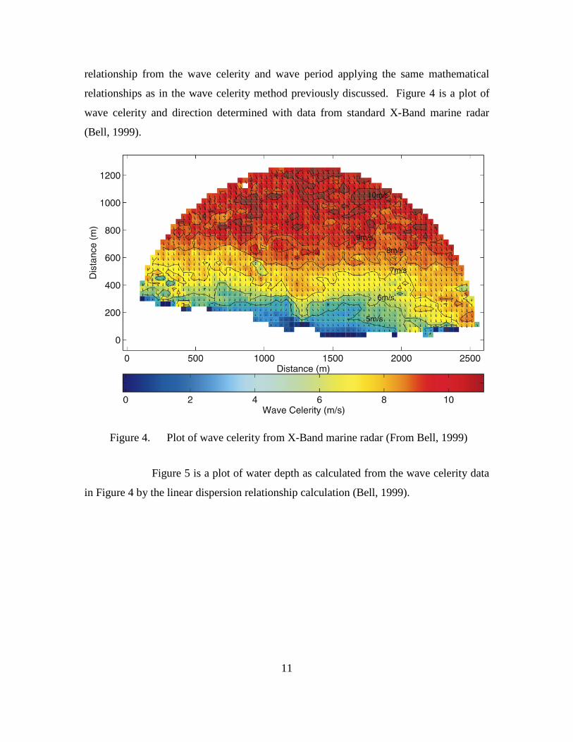
a. X-Band Marine Radar

X-Band marine radars can be used to image the sea surface, and then the

resulting “sea clutter” on the radar image sequences can be exploited to determine the

two-dimensional wave spectra. A three-dimensional Fourier Transform analyses, on a

sequence of radar images, maps wave celerity and direction. Wave period can also be

determined from the radar data. Estimated depth is calculated by the linear dispersion

11

relationship from the wave celerity and wave period applying the same mathematical

relationships as in the wave celerity method previously discussed. Figure 4 is a plot of

wave celerity and direction determined with data from standard X-Band marine radar

(Bell, 1999).

Figure 4. Plot of wave celerity from X-Band marine radar (From Bell, 1999)

Figure 5 is a plot of water depth as calculated from the wave celerity data

in Figure 4 by the linear dispersion relationship calculation (Bell, 1999).

12

Figure 5. Plot of water depth calculated from X-Band radar data (From Bell, 1999)

A long dwell time, of approximately 100 seconds is required for the three

dimensional Fourier Transform analyses, which is not practical for remote sensing type

platforms. Therefore, a study was conducted from data collected with the Imaging

Science Research radar located on the pier of the U.S. Army Corps of Engineers Field

Research Facility, Duck, NC to test the potential for determining bathymetry for small X-

Band radars mounted on aircraft or Unmanned Aerial Vehicles (UAV) with much smaller

dwell times of approximately 10 seconds (Abileah & Trizna, 2010). The 10-second

dwell time for aircraft is much less than the 100-second dwell time required for the three-

dimensional Fourier analyses, so for this study a two-dimensional Fourier Transform

analyses of the data were used. The two-dimensional Fourier analyses actually results in

a number of advantages over the three-dimensional analyses. Fewer images are required;

in fact depth can be estimated with as few as two images. Also, depth accuracy no longer

depends on time; it only depends on the signal to noise ratio (SNR). In fact, if the SNR is

high enough depth can be accurately determined with as few as two images and a dwell

13

time as short as ten seconds. Figure 6 is a plot of water depth calculated from X-Band

radar data estimated with two-dimensional Fourier analyses and overlaid on an aerial

image of Duck, NC (Abileah & Trizna, 2010).

Figure 6. Plot of water depth calculated from X-Band radar data using 2D analyses (From Abileah & Trizna, 2010)

b. Video Imagery and Wave number

Video imagery can also determine nearshore bathymetry by applying the

linear dispersion relationship for surface gravity waves. The video technique first

estimates the frequency of the wave, which involves the collection of pixel intensity time

series at an array of pixel locations. Average spectrum is then calculated and the spectral

peak is selected as the frequency corresponding to the wave celerity. The cross-shore

wave number is then estimated by analysis of wave phase structure through a frequency

domain complex empirical orthogonal function (CEOF). The wave number is then used

14

to calculate depth by the linear dispersion relationship of surface gravity waves. Figure 7

is a plot of estimated wave angle and water depths for Duck, NC calculated by the video

technique. Figure 7 (b) compares the estimated water depths to the ground truth as

collected by Coastal Research Amphibious Buggy (CRAB) for the same day (Stockdon

& Holman, 2000).

Figure 7. Plot of wave angle and water depth estimates for Duck, NC using video technique (From Stockdon & Holman, 2000)

Decoupling the wave number estimation from the water depth estimation

provides improved spatial resolution and quantitative error predictions, and is well suited

to solve the bathymetry inversion problem (Plant, Holland, & Haller, 2008). This is

accomplished by deriving a formal inverse model that solves for the unknown spatially

variable wave numbers from image sequences vice solving for wave celerity

independently (Plant et al., 2008). One advantage of separating the depth estimation

15

from the wave number estimation is that it results in quantitatively accurate bathymetric

error predictions since each depth estimation is based on independent wave number

estimations (Plant et al., 2008).

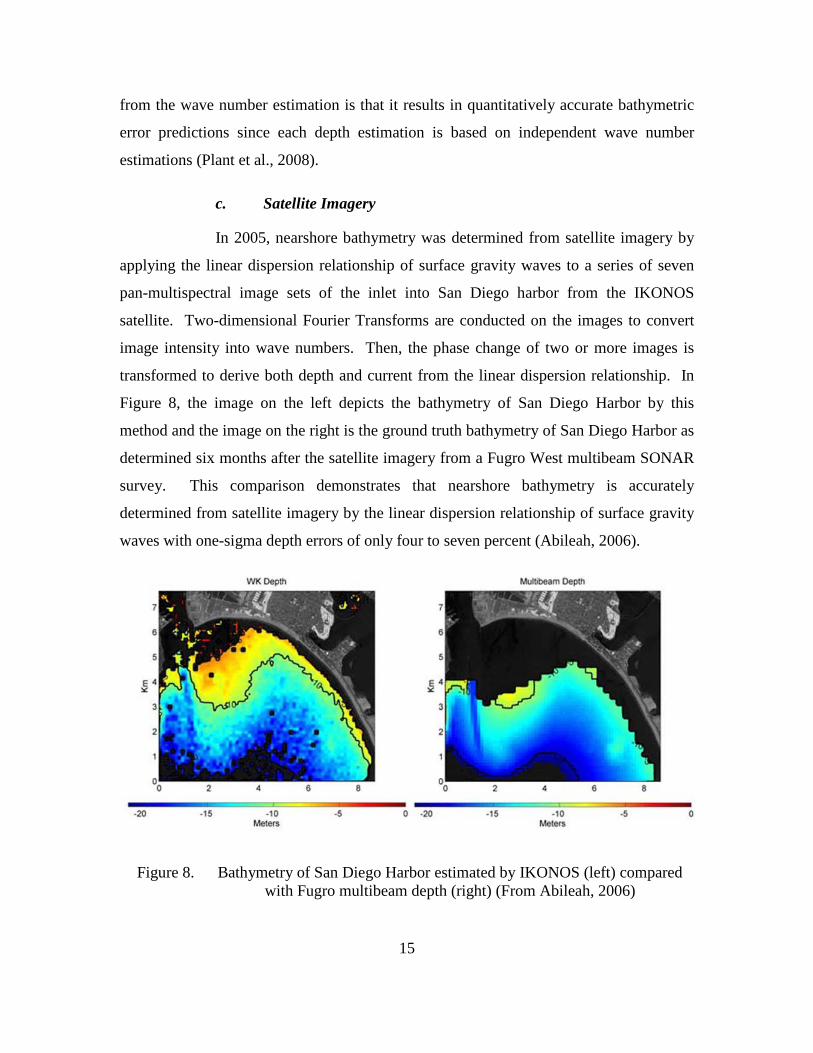
c. Satellite Imagery

In 2005, nearshore bathymetry was determined from satellite imagery by

applying the linear dispersion relationship of surface gravity waves to a series of seven

pan-multispectral image sets of the inlet into San Diego harbor from the IKONOS

satellite. Two-dimensional Fourier Transforms are conducted on the images to convert

image intensity into wave numbers. Then, the phase change of two or more images is

transformed to derive both depth and current from the linear dispersion relationship. In

Figure 8, the image on the left depicts the bathymetry of San Diego Harbor by this

method and the image on the right is the ground truth bathymetry of San Diego Harbor as

determined six months after the satellite imagery from a Fugro West multibeam SONAR

survey. This comparison demonstrates that nearshore bathymetry is accurately

determined from satellite imagery by the linear dispersion relationship of surface gravity

waves with one-sigma depth errors of only four to seven percent (Abileah, 2006).

Figure 8. Bathymetry of San Diego Harbor estimated by IKONOS (left) compared with Fugro multibeam depth (right) (From Abileah, 2006)

16

d. Neuro-Fuzzy Technique

The Neuro-fuzzy technique is an optical depth technique that depends on

an Adaptive-Network-based Fuzzy Inference System (ANFIS) to determine nearshore

bathymetry from multispectral satellite images. An adaptive network is a feed-forward

neural network where each node performs a specific function and no weights associated

to the links between different nodes (Corucci, Masini, & Cococcioni, 2011). This avoids

systematic uncertainties because the algorithm is trained only on real data. Adaptive

networks rely on a collection of input-output data pairs in order to determine the model

structure. In this case the three Quickbird visible bands are the input and estimated depth

is the system output. Accurate bathymetry of the area off the coast of Grosseto, Italy was

determined by this method from two multispectral Quickbird images. The accuracy

obtained by this method was comparable to the accuracy achieved by the linear

dispersion relationship applied to the IKONOS images. However, the ANFIS method

requires a significant amount of predetermined depths to represent the desired output

from the system. These predetermined depths are then divided into three datasets: a test

set, ANFIS validation set, and ANFIS training set (Corucci et al., 2011). This is not

practical when dealing with denied or hostile areas, thus making this method impractical

for an operational capability to determine bathymetry of denied or hostile areas in support

of amphibious operations or mine warfare planning. Figure 9 is a plot of the estimated

depth as determined by ANFIS from the 2008 Quickbird image of Grosseto, Italy, versus

the predetermined depths. The 2008 image is the more realistic of the two images as

there were limited number of predetermined depths associated with that image (Corucci

et al., 2011).

17

Figure 9. Plot of estimated depth by ANFIS versus predetermined depth (From Corucci et al., 2011)

B. THEORY

1. Periodic Waves

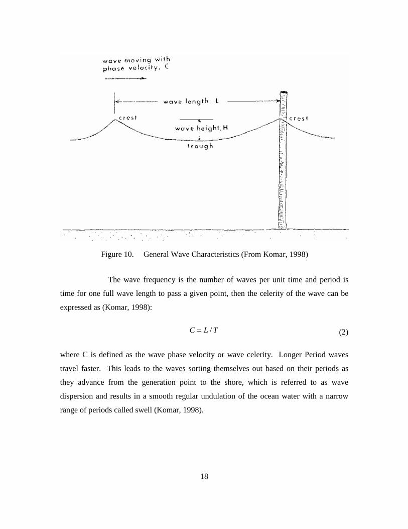
All periodic waves are characterized by the same key parameters: wave length

(L), the horizontal distance from crest to crest; wave height (H), the vertical distance

from trough to crest; and period (T), the time interval between the appearances of

successive crests at the same point. Figure 10 is a graphical depiction of these key

parameters. The frequency (f) of a wave is defined as the number of waves per unit time

and is expressed as (Komar, 1998; Caruthers et al., 1985):

1/f T= (1)

18

Figure 10. General Wave Characteristics (From Komar, 1998)

The wave frequency is the number of waves per unit time and period is

time for one full wave length to pass a given point, then the celerity of the wave can be

expressed as (Komar, 1998):

/C L T= (2)

where C is defined as the wave phase velocity or wave celerity. Longer Period waves

travel faster. This leads to the waves sorting themselves out based on their periods as

they advance from the generation point to the shore, which is referred to as wave

dispersion and results in a smooth regular undulation of the ocean water with a narrow

range of periods called swell (Komar, 1998).

19

2. Linear Airy-Wave

Linear Airy-wave theory is the simplest of the wave theories. For this theory it is

assumed that wave height is much smaller than both the wave length and depth. A

fundamental relationship derived from Linear Airy-wave theory is the dispersion

equation (Komar, 1998):

2 tanh( )gk khσ = (3)

where 2 / Tσ π= is the angular frequency, g is the acceleration due to gravity, 2 /k Lπ=

is the wave number, and h is the water depth. Substituting in the expressions for σ and k

yields (Komar, 1998):

2 2tanh2g hL T

Lπ

π =

(4)

In deep water, where the wave length is small as compared to the depth

( 0 / 2h L> ), the expression 2 hLπ

becomes large thus 2tanh 1hLπ ≈

and Equation (4)

can be reduced to (Komar, 1998):

20 2

gL Tπ

= (5)

Now substituting Equation (5) into Equation (1), we can now write an expression

for the deep water wave celerity:

0 2gC Tπ

= (6)

For deep water waves, wave celerity and wave length are constant and only

depend on the period, wave height is also constant. Deep water waves do not feel the

bottom and therefore are unaffected by the depth as shown in Figure 11 (Komar, 1998).

20

As the waves continue to propagate toward shore, they will begin to feel the

bottom at a depth equal to approximately one half their wave length. At this point, the

deep water expression can no longer be applied (Komar, 1998).

Once the waves reach shallow water where 0 / 20h L< , 2tanh hLπ

approaches

2 hLπ

and Equation 4 can be reduced to the shallow expressions (Komar, 1998):

sL T gh= (7) sC gh= (8)

For shallow water waves, wave celerity and wave length depend only on depth

and period remains constant. Thus, as waves enter shallow water, wave celerity

decreases, wave length decreases, wave height increases and period does not change as

shown in Figure 11 (Komar, 1998).

In the intermediate depth range, where 0 0/ 4 / 20L h L> > , Equation 4 must be

used. For waves in the intermediate depth range, wave celerity and wave length decrease

as depth tends to decrease, while wave height increase as shown in Figure 11 (Komar,

1998).

21

Figure 11. Linear Airy-wave approximations for varying depths (After Komar, 1998)

Table 1 summarizes the principal equations of interest derived from Linear Airy-

wave theory.

22

Table 1. Equations derived from Linear Airy-wave theory (After Komar, 1998)

Parameter General Expression Deep Water Shallow Water

Surface elevation ( , ) cos( )

2Hx t kx tη σ= −

Phase celerity 2tanh2gT hC

Lπ

π =

0 2gTCπ

= sC gh=

Wave length 2 2tanh2gT hL

Lπ

π =

2

0 2gTLπ

= sL T gh=

Horizontal orbital

diameter 0cosh[ ( )]

sinh( )k z hd H

kh+

= 0kzd He=

2 2sHL HT gdh hπ π

= =

Vertical orbital

diameter 0sinh[ ( )]

sinh( )k z hs H

kh+

= 0kzs He= 0s =

Horizontal orbital

velocity 0cosh[ ( )] cos( )

sinh( )k z hHu kx t

T khπ σ+

= − cos( )kzHu e kx tTπ σ= − cos( )

2H gu kx t

hσ= −

Vertical orbital

velocity 0sinh[ ( )] sin( )

sinh( )k z hHw kx t

T khπ σ+

= − sin( )kzHw e kx tTπ σ= −

0w =

23

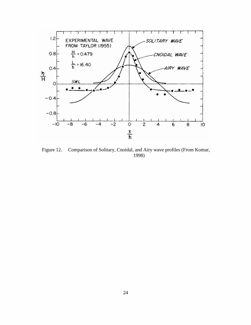
3. Cnoidal and Solitary Wave

Linear Airy-wave theory begins to break down when waves enter into very

shallow water as the ratio H/h approaches unity, and the assumption that H is much

smaller than both L and h is no longer valid (Komar, 1998). This is particularly true in

the surf zone where wave height increases wave celerity (Holland, 2001). The nonlinear

wave processes observed in the surf zone will result in larger wave celerities than

predicted by the linear dispersion relation, resulting in over estimation of depths. In order

to improve the accuracy of depth estimations in the surf zone, a higher order wave theory

should be applied (Bell, 1999).

Cnoidal wave theory should be utilized for waves in the surf zone. However, this

theory is seldom employed due the complexity of the analyses. The expression for

Cnoidal wave celerity is:

( ))c g h Hα= + (9)

where α is a function of Ursell number, ( )2 3/rU H k h= (Komar, 1998). The Ursell

number is a dimensionless parameter used in fluid dynamics to indicate the nonlinearity

of long surface gravity waves on a fluid layer. Solitary wave theory is a limiting case of

the Cnoidal wave theory where 1α = (Holland, 2001). Solitary wave consist of a single

crest and does not have wave period or wave length associated with it (Komar, 1998).

Solitary wave theory accounts for the effects of wave height on wave celerity but

removes the complicated function of Ursell number (Stockdon & Holman, 2000). Thus,

the equation for wave celerity for a solitary wave is:

( )c g h H= + (10)

Figure 12 compares the theoretical wave forms based on Solitary, Cnoidal, and

Linear Airy-wave theories.

24

Figure 12. Comparison of Solitary, Cnoidal, and Airy wave profiles (From Komar, 1998)

25

III. PROBLEM

A. DEFINITION

The capability to remotely determine subaqueous beach profiles of remote,

denied, or hostile areas is critical to providing proper IPE in support of amphibious

operations, mine warfare, and/or HADR planning. “The Navy, in support of amphibious

operations, also requires the ability to remotely and surreptitiously determine the

bathymetry profile of the ocean near amphibious landing zones” (OPNAV N2/N6, 2010).

Remote sensing satellites in LEO provide the best access into these areas. The problem

lies in determining the best method for producing subaqueous beach profiles from remote

sensing data. The wave celerity method by the linear dispersion relationship for surface

gravity waves is a convenient method to accurately estimate nearshore subaqueous beach

profiles, but it requires 2-meter resolution in order to resolve the waves and the ability to

obtain multiple images in short succession.

This study was conducted as a proof of concept to demonstrate that commercial

satellite imagery has sufficient capability to meet the above requirements, and solve the

problem of determining bathymetric profiles of denied or hostile areas. This study used

multispectral imagery acquired by the WorldView-2 satellite to determine the

bathymetric profile of the coastal area near Camp Pendleton, California.

B. MATERIALS

1. WorldView-2 Sensor

WorldView-2 satellite collected ten images in rapid succession of the coastal area

off Camp Pendleton. WorldView-2 is a high resolution 8-band multispectral commercial

imaging satellite owned and operated by DigitalGlobe (Figure 13). It was launched in

October 2009. WorldView-2 is capable of 46 cm panchromatic resolution at nadir and

1.85 m multispectral resolution at nadir (DigitalGlobe, 2011).

26

Figure 13. WorldView-2 Satellite (From DigitalGlobe)

WorldView-2 is the first satellite to combine high resolution panchromatic with 8-

band multispectral sensor capabilities giving it significant spectral performance

improvement over the other two satellites in DigitalGlobe’s fleet, QuickBird and

WorldView-1. In addition to the four standard color bands of blue, green, red, and near

infrared, WorldView-2 adds four new color bands: coastal blue, yellow, red edge, and a

second band of near infrared. Figure 14 shows wave lengths covered by each band as

well as, the increased spectral coverage as compared to the other two DigitalGlobe

satellites (DigitalGlobe, 2010; DigitalGlobe, 2010; DigitalGlobe, 2011).

27

Figure 14. DigitalGlobe satellite spectral coverage (From DigitalGlobe, 2010)

The WorldView-2 satellite can achieve an acceleration of 1.43 deg/s/s and a rate

of 3.86 deg/s allowing it to slew 200 km in 10 seconds. This increased retargeting agility

allows for multiple images of the same area to be taken in rapid succession. Table 2 lists

key parameters and specifications for the WorldView-2 satellite.

Table 2. WorldView-2 Specifications (After DigitalGlobe, 2011)

28

2. The Environment for Visualizing Images 4.7 (ENVI)

The Environment for Visualizing Images software version 4.7 was used in this

study to process the WorldView-2 imagery in order to resolve the wave crest. ENVI 4.7

is a software application produced by ITT Visual Information Solutions for processing

and analyzing geospatial imagery. ENVI 4.7 contains a number of features, functionality

and tools for extracting information from geospatial imagery (ENVI, IDL, & Industry

Brochures from ITT Visual Information Solutions). For this study, features such as;

change detection, Fourier Transforms, Principal Component Transforms, image

registration, filtering, and measurement tools extracted the needed information from the

WorldView-2 imagery.

3. USGS Digital Elevation Model for Southern California

The USGS DEM for Southern California data series 487 provided ground truth

data for this study. The estimated depths calculated for this study were compared to this

USGS DEM to determine accuracy of the methods. This DEM was constructed in 2009

by integrating over forty of the most recent bathymetric and topographic data sets

collected by LIDAR, multibean and single beam SONAR, and Interferometric Synthetic

Aperture Radar (IfSAR). Forty-five individual DEMs were constructed from these

datasets. Figure 15 shows the location of these 45 DEMs, and Table 3 is a list of the

DEM identifiers and respective locations of each. For this study, DEM sd10 was used

(Barnard & Hoover, 2010).

29

Figure 15. USGS location map and identifiers (IDs) for the 45 DEMs (From Barnard & Hoover, 2010)

Table 3. USGS Individual DEM names and locations (From Barnard & Hoover, 2010)

30


31

IV. METHODS AND OBSERVATIONS

A. WORLDVIEW-2 IMAGERY OF CAMP PENDLETON

1. Collection

The imagery of the littoral region near Camp Pendleton, CA was collected on

March 24, 2010, by DigitalGlobe’s WorldView-2 satellite. Ten panchromatic and

multispectral images were collected in rapid succession during a single pass. Figure 16

shows a movie of the collection simulation created by Satellite Tool Kit (STK) from

Analytical Graphics, Inc. (AGI).

Figure 16. STK simulation of WorldView-2 Camp Pendleton area collection (From

McCarthy & Naval Postgraduate School [U.S.], 2010)

32

DigitalGlobe provided the images in ortho-ready standard 2A format and

geographic latitude/longitude coordinates. Each of the ten imagery products were

delivered as three scenes approximately full swath width of 16.4 km and cut into 14 km

lengths with at least 1.8 km overlap between each scene (DigitalGlobe). The total

imagery product for each of the ten images consisted of three scenes identified as R1C1,

R2C1, and R3C1. Figure 17 shows the basic imagery products that are divided up and

delivered as scenes by DigitialGlobe. Figure 18 is a Google Earth representation of the

layout of scenes R1C1, R2C1, and R3C1 from the basic imagery product of the first

image of the Camp Pendleton imagery. The blue shaded area represents scene R1C1, the

green shaded area represents scene R2C1, and the red shaded area represents the scene

R3C1.

Figure 17. Physical Structure of Imagery Scenes (From DigitalGlobe)

33

Figure 18. Google Earth representation of WorldView-2 data for Camp Pendleton area (From McCarthy & Naval Postgraduate School (U.S.), 2010)

Table 4 is a summary of the information derived from the image meta-data for

each of the ten images collected. The last column in Table 4 shows the time interval

between each of the successive images in this data set.

34

Table 4. Summary of image meta-data information (From McCarthy & Naval Postgraduate School, 2010)

2. Image Processing

a. Image Registration

The imagery was provided in ortho-ready standard 2A format as

previously mentioned. In this format, the image is projected onto a reference ellipsoid

using a constant base elevation with no topographic relief applied. This makes the

imagery suitable for orthorectification (DigitalGlobe). Images P002, P007 and P009

were registered to the middle image P008 (Table 4) in ENVI by the resampling, scaling,

and translation (RST) method with nearest neighbor resampling. Four ground reference

points were selected near the waterline for the registration of the images. The first

ground reference point was located in the upper left corner of the image, the second near

the bottom of the image, the third and fourth near the center of the coastline. Figure 19

shows the locations of the ground reference points on an example image.

35

Figure 19. Ground reference point location for image to image registration (From McCarthy & Naval Postgraduate School [U.S.], 2010)

b. Image Rotation and Resizing

Next, the three registered images were rotated 131 degrees in an effort to

align the coastline with the horizontal axis in order to allow the vertical profile function

to measure wave lengths and wave distances. Figure 20 shows the results of this rotation.

Figure 20. Image rotation 131 degrees

36

After the images were rotated, they were then resized with ENVI to focus

on the coast line and shallow water area for bathymetry determination. All three images

were resized using a spatial subset of the image reducing the number of lines from 17404

to 2500. This was done to reduce the size of the image in order to make it more

manageable for data extraction. Figure 21 shows the final size and layout of the images

used for bathymetry determination following the initial image processing in ENVI.

Figure 21. Resized Image

3. Principal Component Transforms

Principal component transforms were performed on images P007 and P009 in

ENVI to aid in wave detection. Principle component transform is a transformation

process that rotates the data space into a coordinate system in which the different bands

are uncorrelated to aid in target detection (Olsen, 2007). The eight band multispectral

imagery provided by the WorldView-2 gave increased degrees of freedom for the

principal component transforms to aid in target detection of wave crest. Figure 22 shows

each of the eight original bands for image P007. Figure 23 shows the eight principal

component bands for image P007. Principal component 4 clearly resolves the wave crest

in the surf zone as distinct narrow lines.

37

Figure 22. Original Eight Bands for image P007

Figure 23. Eight Principal Component Banks for image P007

B. SURF ZONE

The resulting principal component four images from both images P007 and P009

where used to create a change detection image in order to determine wave celerity in the

surf zone. This was accomplished by placing principal component four from image P007

into both the red and green inputs and then placing principal component four from image

38

P009 into the blue input. Figure 24 shows the resulting change detection image. The

blue lines are the highlighted wave crest from principal component four from image P007

and the yellow lines are the highlighted wave crest from principal component four from

image P009. Distance between the blue and yellow wave crest was then determined with

the ENVI measurement tool. Wave celerity was then calculated using the time between

images from Table 4. The linear dispersion relation for surface gravity waves was then

applied to determine estimated depths. Wave height was observed to be minimal during

the time frames of these particular images.

Figure 24. Change detection image for surf zone

C. OUTSIDE OF THE SURF ZONE

The principal component transform did not clearly resolve the wave crest in the

shallow water as it did in the surf zone. Therefore, a change detection image was unable

to be created for the area outside the surf zone and another method of determining wave

celerity had to be determined. For the region outside the surf zone, the waves were first

resolved by representing both images P007 and P009 in an RGB color representation of

bands seven, six, and five in ENVI. These bands do not penetrate the water, resulting in

increased surface wave contrast (Abileah, 2006). Then the images were enhanced by

either image equalization or image linear two percent enhancement in ENVI to highlight

39

the wave crest. Figure 25 shows the results of this representation and enhancement of the

waves.

Figure 25. Image P007 (left) and P009 (right) represented by 765 bands in RGB and

image equalization enhancement

The two images were linked by both linking the displays and geographic link in

ENVI in order to ensure that the same area was being viewed in each image. A spatial

profile was performed on each image with the vertical profile in ENVI to identify the

center of the wave crest. The coordinates of the crest centers were identified with the

cursor location tool in ENVI. Distance between the corresponding wave crest was then

determined by the ENVI measurement tool. Wave celerity was then calculated using the

time between images from Table 4. The linear dispersion relation for surface gravity

waves was then applied to determine estimated depths.

40


41

V. ANALYSIS

A. SURF ZONE

Depth was estimated in the Surf Zone by the wave celerity method. The wave

celerity was determined by measuring the distance the wave traveled between image

P007 and P009 and then dividing by the elapsed time between the two images as obtained

from Table 4. This was accomplished by measuring the distance from the blue line to the

yellow line in the change detection image with the ENVI measurement tool as shown in

Figure 26.

Figure 26. Calculating wave distance using ENVI measurement tool for surf zone

42

Once the wave celerity was calculated for each of the depth data points Equation

8 was rearranged to produce the equation:

2ch

g= (11)

to estimate the depth for each of the depth data points. Depth was estimated for fifty

depth data points in the surf zone along the coast off Camp Pendleton. The actual points

where the depth was estimated corresponds to the midpoint between the blue and yellow

lines in the change detection image as indicated by the green triangle in Figure 26. The

estimated depths were compared to the ground truth data. This was accomplished by first

geographically linking the USGS DEM sd10 image to the change detection image in

ENVI. The depth data point was located on the change detection image with the Pixel

Locator tool in ENVI by the pixel coordinates associated with each depth data point.

Since the two images were geographically linked the locator on the USGS image located

the corresponding geographical point on the USGS image and the ground truth depth was

determined from the data field of the Cursor Location/Value tool associated with the

USGS image in ENVI as shown in Figure 27.

Figure 27. Ground Truth determination from USGS DEM sd10 for surf zone

The estimated depths were plotted against the ground truth depths to determine

the accuracy of the wave celerity method in the surf zone (Figure 28).

43

Figure 28. Plot of estimated depth versus ground truth depth in the surf zone

44

Figure 28 shows that on average the wave celerity method reflected a 5.2 percent

error in the surf zone based on the equation for the best fit curve for the fifty depth data

points with a coefficient of determination (R2) of 0.59. The perfect model would have

resulted in an equation with a slope of 1.0 and R2 of 1.0. Sources of error include, not

accounting for the wave heights in the surf zone as discussed in Chapter II, and there is a

plus or minus ten percent uncertainty in the estimated depth associated with the location

measurement error of plus or minus one pixel (2.4 m). The R2 value of 0.59 says that the

regression line is a good fit to the data and that it is a fair representative model. It must

be noted, however, that a few individual depth estimations resulted in nearly a fifty

percent over estimation of water depth. All estimated depths were within plus or minus

one meter of ground truth and most were within plus or minus a half meter of ground

truth. Table 6 in Appendix contains the specific results for each of the depth data points.

B. OUTSIDE OF THE SURF ZONE

Depth was estimated outside the surf zone by the wave celerity method as well;

however, a change detection image for this region was not able to be produced as

discussed in Chapter IV. Wave celerity was determined by measuring the distance the

wave traveled between image P007 and P009 and then dividing by the elapsed time

between the two images as obtained from Table 4. This was accomplished outside the

surf zone by determining the pixel coordinates of the wave crest in both image P007 and

P009 as discussed in Chapter IV and then using the ENVI measurement tool to measure

the distance between those pixel coordinates to determine the distance the wave traveled

between images as shown in Figure 29.

45

Figure 29. Calculating wave distance for outside the surf zone

Once the wave celerity was calculated for each of the depth data points Equation

4 was then rearranged to produce the equation:

2

2arctanh2

L LhgTπ

π =

(12)

to estimate the depth for each location. Depth was estimated for twenty eight points

outside the surf zone off the coast of Camp Pendleton. The points where the depth was

estimated corresponds to the midpoint between the pixel coordinate associated with the

wave crest in image P007 and the pixel coordinate associated with the wave crest in

image P009 as indicated by the green triangle in Figure 29. The estimated depths for

each of these points was compared to the ground truth data as determined from the USGS

DEM sd10 in ENVI. This was accomplished by first geographically linking the USGS

DEM sd10 image to both images P007 and P009 in ENVI. The depth data point was

located on image P007 with the Pixel Locator tool in ENVI by the pixel coordinates

associated with each depth data point. Since the two images were geographically linked

the locator on the USGS image located the corresponding geographical point on the

46

USGS image and the ground truth depth was determined from the data field of the Cursor

Location/Value tool associated with the USGS image in ENVI as shown in Figure 30.

Figure 30. Ground Truth determination from USGS DEM for outside the surf zone

The estimated depths were plotted against the ground truth depths for each of the

twenty eight depth data points to determine the accuracy of the wave celerity method

outside the surf zone as shown in Figure 31.

47

Figure 31. Plot of estimated depth versus ground truth depth outside the surf zone

48

Figure 31 shows that on average the wave celerity method outside the surf zone

reflected less than a one percent error based on the equation for the best fit curve for the

twenty eight depth data points with a coefficient of determination (R2) of 0.86. There is

again a plus or minus ten percent uncertainty in the estimated depth associated with the

location measurement error of plus or minus one pixel (2.4 m). This model is much more

accurate than the one determined for the surf zone because as discussed in Chapter II

there is no need to account for wave height in this zone and the linear theory still holds

true. The R2 value of 0.86 says that the regression line is a near perfect fit to the data and

that it is a good representative model. All estimated depths were within plus or minus

one meter of ground truth and most were within plus or minus a half meter of ground

truth. Table 5 in Appendix contains the specific results for each of the depth data points.

49

VI. SUMMARY

WorldView-2 multispectral imagery of the coastal area near Camp Pendleton,

California was used to determine ocean depth for both in the surf zone and outside the

surf zone by the wave celerity method and applying the linear dispersion relationship for

surface gravity waves. The high spatial resolution provided by the multispectral satellite

imagery was more than sufficient to resolve the waves. The high retargeting agility

provided by WorldView-2 allowed for multiple images to be taken in rapid succession of

the same area which in turned allowed for wave celerity to be accurately determined.

The eight bands comprising the multispectral imagery provided for the removal of image

contamination as well as increased degrees of freedom, further improving the image

quality for performing measurements. The images were co-registered, rotated, resized

and principal component transforms performed in ENVI to provide an accurate baseline

of images to conduct measurements and extract data.

Principal component four was found to resolve the wave crest in the surf zone.

Using the principal component four image from both images P007 and P009 a change

detection image was created with an RGB image where principal component four for

image P007 was represented by red and green and principal component four for image

P009 was represented by blue. This produced a single image containing both spatial and

temporal information where waves moved from blue to yellow in the time between

images. This allowed for the accurate measurement of distance traveled by the wave

between the two images from which wave celerity was calculated. The linear dispersion

relationship for surface gravity waves was then applied to estimate the depth in the surf

zone. This method reflected a five percent over estimation of depth on average in the

surf zone, however, there were errors up to fifty percent in some individual estimates.

This is a result of the fact that the linear theory begins to breakdown in the surf zone and

wave height must be accounted for or an over estimation of depth can be expected as

observed here.

None of the principal components clearly resolved the wave crest outside the surf

zone as principal component four did in the surf zone; therefore, a change detection

50

image could not be created for outside the surf zone. Wave celerity for outside the surf

zone was determined by geographically linking images P007 and P009 in ENVI then

determining the location of the corresponding wave crest from image P009 in image

P007. The distance from the wave crest in image P007 to the wave crest in image P009

was accurately measured by the ENVI measurement tool and wave celerity calculated.

The linear dispersion relationship for surface gravity waves was then applied, as with the

surf zone data, to estimate the depth in the region outside the surf zone. This method

reflected less than a one percent error on average outside the surf zone with no more than

a seven percent error for any individual estimate.

51

VII. CONCLUSION

Nearshore subaqueous beach profile was accurately determined both in the surf

zone and outside the surf zone from WorldView-2 multispectral imagery of the coastal

area near Camp Pendleton, California by the wave celerity method and applying the

linear dispersion relationship for surface gravity waves. The estimated depths for each of

the depth data points compared favorably with the ground truth bathymetry as determined

from the USGS DEM of the same area and were more than sufficiently accurate for the

purposes of IPE, especially in the region outside the surf zone. This method resulted in

larger discrepancies from ground truth in the surf zone due to the fact that the linear

theory begins to break down at this point, however the results were still within one meter

of ground truth and in most instances were within a half meter. The results in the surf

zone are sufficiently accurate at these shallow depths for the purposes of IPE in support

of amphibious operations, HADR, and mine warfare planning operations.

The wave period method was determined to not be a viable method for

determining nearshore bathymetry from space. This conclusion was drawn based on the

fact that due to the wave dispersion process it cannot be assumed that the deep water

wave period observed in an image is the same deep water period for the wave group in

the shallow water or surf zones.

This study demonstrates that determining nearshore bathymetry from space by the

wave celerity method is a viable solution for determining nearshore bathymetry of hostile

or denied areas. Based on this proof of concept additional work needs to be done in order

to automate the process so that it can be delivered to the fleet as an operational tool.

Future work should include research and development of algorithms that can

automatically conduct exhaustive depth computations from multiple images by accurately

determining either the wave celerity or wave number for an extensive number of depth

data points common to all images. From these computations a subaqueous beach profile

should be created that can be used by the fleet for IPE in support of amphibious

operations, HADR, and mine warfare planning.

52


53

APPENDIX

Table 5. Data table for depth data points outside of the surf zone

54

Table 6. Data table for surf zone depth data points

55

LIST OF REFERENCES

Abileah, R., & Trizna, D. B. (2010). Shallow water bathymetry with an incoherent X-band radar using small (smaller) space-time image cubes. Paper presented at the Geoscience and Remote Sensing Symposium (IGARSS), 2010 IEEE International, 4330–4333. Abileah, R. (2006). Mapping shallow water depth from satellite. Paper presented at the ASPRS 2006 Annual Conference, Reno, Nevada.

Barnard, P. L., & Hoover, D. (2010). A seamless, high-resolution, coastal digital elevation model (DEM) for Southern California. U.S.Geological Survey Data Series, 8. Retrieved from http://search.proquest.com/docview/742920456?accountid=12702; http://pubs.usgs.gov/ds/487/

Bell, P. S. (1999). Shallow water bathymetry derived from an analysis of X-band marine radar images of waves. Coastal Engineering, 37(3-4), 513–527. doi: 10.1016/S0378-3839(99)00041-1

Caruthers, J. W., Arnone, R. A., Howard, W., Haney, C., & Durham, D., L. (1985). Water Depth Determination Using Wave Refraction Analysis of Aerial Photography. (NORDA No. 110). NSTL, Mississippi: Naval Ocean Research and Development Activity.

Corucci, L., Masini, A., & Cococcioni, M. (2011). Approaching bathymetry estimation from high resolution multispectral satellite images using a neuro-fuzzy technique SPIE. doi:10.1117/1.3569125

DigitalGlobe | DigitalGlobe: Worldview-2 Satellite - 46cm Resolution Retrieved 8/19/2011, 2011, from http://www.digitalglobe.com/index.php/88/WorldView-2

DigitalGlobe, I.DigitalGlobe Core Imagery Products Guide. Unpublished manuscript. Retrieved 8/21/2011, from http://www.digitalglobe.com/file.php/811/DigitalGlobe_Core_Imagery_Products_Guide.pdf

DigitalGlobe, I. (2010). Whitepaper: The benefits of the 8 spectral bands of worldview-2. Unpublished manuscript. Retrieved 8/19/2011, from http://www.digitalglobe.com/downloads/spacecraft/WorldView-2_8-Band_Applications_Whitepaper.pdfhttp://www.digitalglobe.com/downloads/spacecraft/WorldView-2_8-Band_Applications_Whitepaper.pdf

DigitalGlobe, I. (2011). DigitalGlobe constellation - Worldview-2 imaging satellite. Unpublished manuscript. Retrieved 8/19/2011, from http://www.digitalglobe.com/downloads/spacecraft/WorldView2-DS-WV2.pdf

56

ENVI, IDL, & Industry Brochures from ITT Visual Information Solutions Retrieved 8/21/2011, 2011, from http://www.ittvis.com/language/en-U.S./ProductsServices/ProductBrochures.aspx

Gao, J. (2009). Bathymetric mapping by means of remote sensing: methods, accuracy and limitations. Progress in Physical Geography, 33(1), 103–116. doi:10.1177/0309133309105657

Holland, K. T. (2001). Correction to “application of the linear dispersion relation with respect to depth inversion and remotely sensed imagery.” Geoscience and Remote Sensing, IEEE Transactions on, 39(10), 2319–2319.

Komar, P. D. (1998). Beach processes and sedimentation (2nd ed.). Upper Saddle River, N.J: Prentice Hall.

McCarthy, B. L., & Naval Postgraduate School (U.S.). (2010). Coastal bathymetry using 8-color multispectral satellite observation of wave motion [electronic resource]. Monterey, CA: Naval Postgraduate School. Retrieved from http://edocs.nps.edu/npspubs/scholarly/theses/2010/Sep/10Sep%5FMcCarthy.pdf (18.07 MB); http://handle.dtic.mil/100.2/ADA531460

Olsen, R. C. (2007). Remote sensing from air and space. Bellingham, WA: SPIE Press.

OPNAV N2/N6. (2010). Navy Space Capability Needs. (OPNAV N2/N6 Memo 5910 No. 10S150054). Arlington, VA: OPNAV.

Plant, N. G., Holland, K. T., & Haller, M. C. (2008). Ocean Wavenumber Estimation From Wave-Resolving Time Series Imagery. Geoscience and Remote Sensing, IEEE Transactions on, 46(9), 2644–2658.

Stockdon, H. F., & Holman, R. A. (2000). Estimation of wave phase speed and nearshore bathymetry from video imagery. Journal of Geophysical Research, Oceans, 105, 22015–22033. Retrieved from http://search.proquest.com/docview/17718325?accountid=12702

Williams, W. W. (1947). The determination of gradients on enemy-held beaches. The Geographical Journal, 109(1/3), 76–90.

57

INITIAL DISTRIBUTION LIST

1. Defense Technical Information Center Ft. Belvoir, Virginia

2. Dudley Knox Library Naval Postgraduate School Monterey, California

3. Dr. Richard C. Olsen Remote Sensing Center at the Naval Postgraduate School Monterey, California

4. Dr. Jamie MacMahan Naval Postgraduate School Monterey, California

myrick, kenneth b. coastal bathymetry using satellite

Documents