musical soundsdigital synthesis of

Professorial Inaugural Lecture, 26 April 2001

DIGITAL SYNTHESIS OFMUSICAL SOUNDS

B.T.G. TanDepartment of Physics

National University of Singapore

MUSICAL SYNTHESIS

The many music synthesizers and keyboardsavailable today from manufacturers such asYamaha can generate musical sounds which arereasonably close to that of musical instrumentssuch as the clarinet and trumpet.

The generation or synthesis of musical soundsaims to reproduce as closely as possible theharmonic structure of the instrument beingimitated.

1

MUSIC AND VIBRATIONS

All musical notes are the result of vibrations i.e.an object must vibrate to make the air vibrate,giving rise to a sound wave which reaches ourears. We are able to hear sound vibrations fromabout 20Hz to 20,000Hz.

Musical instruments can give rise to a sound waveby:

• Scraping a stretched string and causing it tovibrate i.e. string instruments.

• Blowing into a tube and causing the aircolumn to vibrate - wind instruments.

• Hitting a solid object and causing it tovibrate - percussion instruments.

The nature of the vibration gives each instrumentits particular colour or timbre.

2

TIMBRE AND HARMONICS

The timbre can be shown to be due to theharmonics of the musical sound produced.

For example, a clarinet playing the note A4 willhave a series of harmonics with

1. The first harmonic or fundamental at 440Hz.

2. The second harmonic at double thisfrequency i.e. 880 Hz.

3. The third harmonic at three times i.e. 1320nHz, and so on.

It is the relative strength of the harmonics whichgives the clarinet its characteristic sound.

A trumpet which is playing the same note willalso have its fundamental at 440 Hz, but therelative strength of its harmonics will be differentfrom the clarinet. This gives the trumpet sound adifferent colour or timbre from the clarinet.

3

-

6 Clarinet harmonics

f 2f 3f 4f 5f 6f 7f 8f 9f 10f

harmonicamplitude

frequency

-

6 Trumpet harmonics

f 2f 3f 4f 5f 6f 7f 8f 9f 10f

harmonicamplitude

frequency

f = fundamental, 2f = 1st harmonic, 3f = 2nd harmonic etc

4

TYPES OF MUSICAL SYNTHESIS

• Additive synthesis: The requiredharmonics are generated separately andadded together.

• Subtractive synthesis: A sound rich inharmonics (e.g. white noise) is the startingpoint and filters are used to subtract theundesired harmonics.

• FM synthesis: (invented by John Chowningof Stanford) Two or more waveforms areused, one modulating the frequency of theother, to generate a rich harmonic structure.To obtain the desired harmonics, thefrequencies and amplitudes of the twowaveforms must be optimized.

• Sampling/wavetable synthesis: Thewaveform of an actual musical instrument issampled and its shape stored in memory as aset of wavetables.

5

FM AND RELATED SYNTHESISTECHNIQUES

In (Frequency Modulation) FM synthesis, thefrequency of a sinusoidal carrier wave ismodulated by another sinusoidal waveform to givea complex waveform which is rich in harmonics.

By suitable choice of the frequencies and degreeof modulation, the harmonic structure of theresultant FM waveform can be made toapproximate to that of a desired waveform, suchas that of a musical instrument.

We consider a carrier waveform of circularfrequency ωc which is frequency modulated by asinusoidal waveform of x(t) of circular frequencyωm and amplitude Am:

x(t) = Amcos(ωmt)

6

SYNTHESIS EQUATION FOR FM

The instantaneous frequency f of the carrier wavethus becomes:

f = fc + Amcos(ωmt)

The resultant carrier wave is therefore

x(t) = Acsin(ωc + 2πKf

∫ t

0

Amcos(ωmt′)dt′)

i.e.

x(t) = Acsin(ωct +2πKfAm

ωmsin(ωmt))

If we define the degree of modulation by themodulation index, I as

I =2πKfAm

ωm=

AmKf

fm

we have the basic synthesis equation for FM :

x(t) = A sin[ωc + I sin(ωmt)]

7

BESSEL FUNCTIONS

x(t) can be expressed as a sum of sinusoids offrequency and amplitude given by

x(t) = A∞∑

n=−∞Jn(I) sin(ωc + nωm)t

where Jn(I) are Bessel Functions.

The FM spectrum thus consists of a centralcarrier frequency with symmetrical harmonicsaround it.

-

6

66

66

66

AJ0(I)

AJ1(I)AJ−1(I)

AJ2(I)AJ−2(I)

AJ3(I)AJ−3(I)

fc fc+mfc−m fc+2mfc−2m fc+3mfc−3m

8

REFLECTED HARMONICS

Looking at a typical FM spectrum, as I increases,the number of non-zero harmonics increases. Thespectral envelope is mainly dependent on I, butthe frequencies of the harmonics and the intervalsbetween them are determined by the ωc and ωm.

For example, with I = 1.0, ωc = 200 andωm = 200, we obtain a resulting FM spectrumwith seven harmonics. The harmonics of negativefrequency are reflected from the zero to giveharmonics with opposite phase.

It may happen that some of the reflectedharmonics coincide with the unreflected ones. Inthis example, the -200 Hz harmonic coincideswith the +200 Hz harmonic, and the -400 Hzharmonic conicides with the +400 Hz harmonic.

The resultant FM spectrum has five harmonicswith the +200 Hz and +400 Hz harmonicsreduced in amplitude after reflection.

9

-

6

6666

66

n = 0FM spectrum

200 4000 600-200 800-400

frequency

-

6

666

?

6?

n = 0Reflection of negative frequencies

200

400

0 600 800

frequency

-

66

66

6

n = 0Resulting FM spectrum

200 4000 600 800

frequency

10

HARMONICITY

If the ratio of the carrier frequency andmodulating frequency:

ωc

ωm=

Rc

Rm

and there is a minimum non-zero |Rc − nRm| = 1where n = 1, 2, 3, 4...

then a harmonic spectrum will be obtained wherethe harmonics are multiples a fundamentalfrequency.

Typical examples of such Rc

Rmare:

12 , 1

3 , 14 , 1

5 ...

23 , 3

4 , 45 , 6

7 , 32 , 4

3 , 52 etc

On the other hand if the minimum non-zero|Rc − nRm| 6= 1 where n = 1, 2, 3, 4..., then theharmonics will not be multiples of a fundamentalfrequency.

11

VARIANTS OF FM SYNTHESIS

Asymmetrical FM or AFM synthesis

A parameter rn is inserted thus:

x(t) = A∞∑

n=−∞rnJn(I) sin(ωc + nωm)t

which gives harmonics which are NOTsymmetrical about the carrier frequency.

Hence the harmonics can be more complex andmore like actual harmonics of real instruments.

However the synthesis equation is more complex:

xc(t) = A exp[I

2(r − 1

r) cos(ωmt)]

sin[ωct +I

2(r +

1r) sin(ωmt)]

and hence requires more computation. If r = 1.0,AFM is equivalent to FM.

12

DOUBLE FREQUENCY MODULATION

Instead of one frequency being the carrier and theother the modulator, in double frequencymodulation (DFM) they have equal statusthus:

x(t) = A sin[I1 sin(ω1t) + I2 sin(ω2t)]

where I1 and I2 are the modulation indices of thetwo frequencies and ω1 and ω2 are their respectivefrequencies.

We can show that

x(t) =∑

p

∑q

Jp(I1)Jq(I2) sin(pω1t + qω2t)

where p and q are integers of different parity.

DFM thus generates harmonics of angularfrequency pω1 + qω2. It also generates many moresignificant harmonics than FM, due to theharmonics depending on product of the twoBessel functions instead of the single Besselfunction of FM.

13

-6

66

6666

FM

0

frequency

-6 6

66

6

6

6

6

6

6

6

AFM

0

frequency

-6

66

6666

66 6666

DFM

0

frequency

14

COMPARISON OF AFM AND DFM

DFM is able to generate harmonics of greatercomplexity than FM, but with much lesscomputational load than AFM.

In AFM there are

• two sine functions

• one cosine function

• one exponential function

• five multiplication

• two divisions

• two additions

• one subtraction.

In DFM we have only

• three sine functions

• two multiplications

• one addition

15

OPTIMISATION OF FM PARAMETERS

For FM synthesis, the parameters for the carrierand modulator frequencies i.e.

ωc, ωm and I

have to be optimized for the closest fit to theharmonics of the instrument to be imitated.

For AFM synthesis, the parameters

ωc, ωm, I and r

have to be optimized.

For DFM synthesis, the parameters for the twofrequencies,

I1, I2, ω1 and ω2

have to be optimized.

This has normally been done by trial and error,which is a tedious and lengthy process.

16

FM, AFM, DFM SOLUTION SPACES

For FM, AFM, and DFM synthesis, the relevantparameters which determine the spectrum of thesynthesized waveform can be evaluated by afitness parameter.

The smaller the fitness for a given set ofparameters, the closer is the resultant spectrumto the desired one.

The fitness can be plotted as a function of therelevant parameters in a solution space. Thelowest valley of this space determines the set ofparameters which generate the waveform having aspectrum most closely resembling that of themusical instrument to be synthesized.

The objective of optimization is thus to find theset of parameters which gives the best fitnessvalue.

17

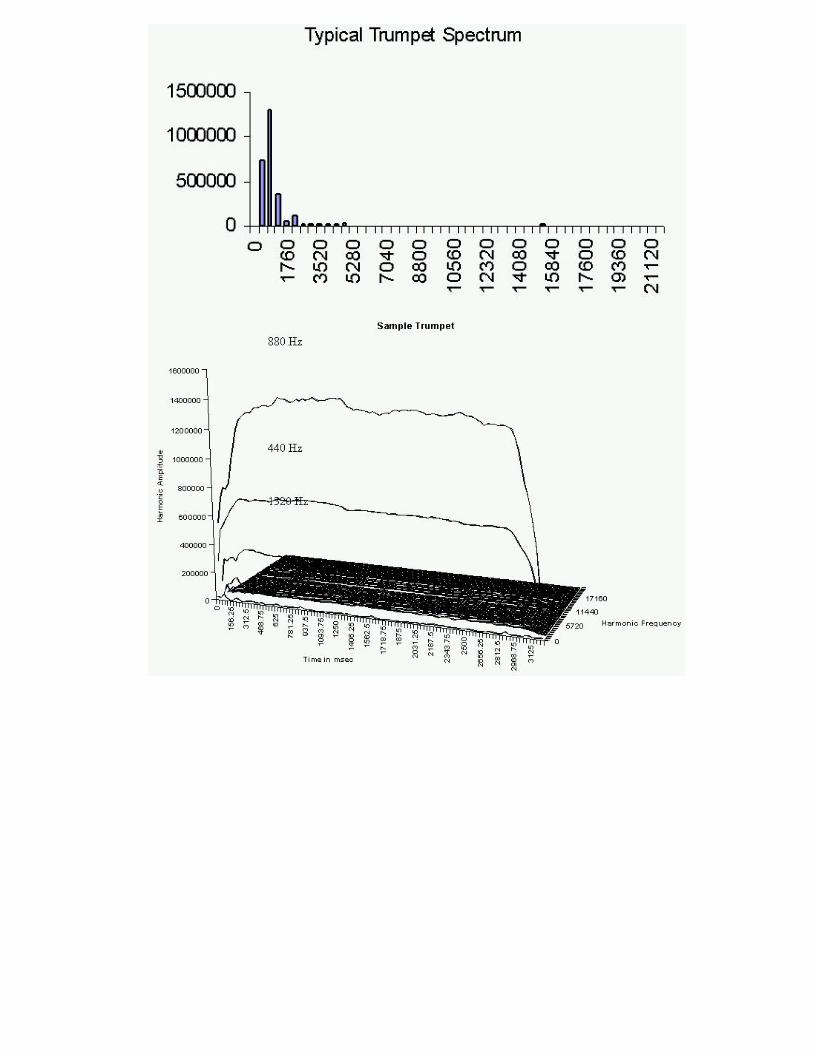
REAL MUSICAL INSTRUMENTSAMPLES

The real musical instrument samples wereobtained from the standard McGill UniversityMaster Samples (MUMS) CD. This CDcontains recordings of musical instruments playingnotes at standard frequencies such as A=440 Hz.

Selected recordings were analyzed by dividingeach note into time frames of 31.25 milliseconds.This time frame was then sampled and fed into a1024 point FFT program.

For a single time frame, the plot of the amplitudesof the harmonics versus their frequency shows theenvelope or shape of the harmonic spectrum.

By plotting the harmonic amplitudes for all thetime frames successively, it is possible to obtain aplot of the spectrum as it changes through theduration of the musical note.

18

FM SOLUTION SPACE

Having obtained a plot of the harmonics for aparticular time frame, we can then attempt tosynthesize the musical instrument tone using FM,AFM or DFM synthesis to replicate the harmonicspectrum as closely as possible.

For example, for FM synthesis, we can vary threeparameters: ωc, ωm and I. For convenience, wedefine fc = ωc

2π and fm = ωm

2π .

In practice, for a tone at A=440 Hz, we fixfc = 440 and fm = 440. We then need to find thevalue of I for which the fitness of the synthesizednote is at an optimum value.

The nature of the optimization problem can bemore clearly shown by plotting the value of thefitness for a range of values of I. For example, forthe trumpet tone, it can be seen from such a plotthat the minimum fitness occurs at I = 4.65.

19

AFM AND DFM SOLUTION SPACES

Similar solution spaces can be plotted for AFMand DFM synthesis.

We consider the same trumpet tone at A = 440Hz.

For AFM synthesis, we can fix f1 = 440 andf2 = 880. The solution space is then a plot of thefitness value for varying I and r. The minimumfitness occurs at I = 0.55 and r = 2.10.

Likewise, for DFM synthesis, we fix f1 = 440 andf2 = 880 to plot the fitness against I1 and I2.From the solution space, the minimum fitnessoccurs at I1 = 3.05 and I2 = 1.40

The FM, AFM and DFM all employ a singleoperator. By employing two or more operators, itis possible to obtain solution spaces withminimum fitness of even lower values.

20

Chart1

Page 1

0.0

0

0.3

5

0.7

0

1.0

5

1.4

0

1.7

5

2.1

0

2.4

5

2.8

0

3.1

5

3.5

0

3.8

5

4.2

0

4.5

5

4.9

0

5.2

5

5.6

0

5.9

5

6.3

0

6.6

5

7.0

0

7.3

5

7.7

0

8.0

5

8.4

0

8.7

5

9.1

0

9.4

5

9.8

0

10

.15

10

.50

10

.85

11

.20

11

.55

11

.90

1

1.00E-03

1.00E-02

1.00E-01

1.00E+00

1.00E+01

Fitn

ess

Index Harmonic

FM Solution Space for Trumpet at 2000ms

Min at Index = 4.65 & freq2 = 440Hz when Freq1 = 440Hz

Chart1

Page 1

0.05

0.30

0.55

0.80

1.05

1.30

1.55

1.80

2.05

2.30

2.55

2.80

3.05

3.30

3.55

3.80

4.05

4.30

4.55

4.80

5.05

5.30

0.05

0.40

0.75

1.10

1.45

1.80

2.15

2.50

2.85

3.20

3.553.90

4.25

1.00E-03

1.00E-02

1.00E-01

1.00E+00

1.00E+01

1.00E+02

1.00E+03

1.00E+04

1.00E+05

1.00E+06

1.00E+07

1.00E+08

1.00E+09

1.00E+10

1.00E+11

1.00E+12

1.00E+13

1.00E+14

1.00E+15

Fitn

ess

Index

Ratio

AFM Solution Space for Trumpet at 2000msMin at R=2.10 I=0.55 f1=440 f2=880

0.0

5

0.4

0

0.7

5

1.10 1.4

5

1.8

0

2.1

5

2.5

0

2.8

5

3.2

0

3.5

5

3.9

0

4.2

5

0.05

0.40

0.75

1.10

1.45

1.80

2.15

2.50

2.85

3.20

3.553.90

4.254.60

4.95

1.00E-03

1.00E-02

1.00E-01

1.00E+00

1.00E+01

1.00E+02

Fitn

ess

Index2

Index1

DFM Solution Space for Trumpet at 2000msMin at I1=3.05 I2=1.40 f1=440 f2=880Hz

SOLUTION SPACES FOR THE VIOLIN

For comparison we have also plotted solutionspaces for the violin for FM, AFM and DFM (forsingle operators).

FM synthesis:

fc = fm = 440

Minimum fitness occurs at I = 0.8

AFM synthesis:

fc = fm = 440

Minimum fitness occurs at I = 0.1 and r = 0.51

DFM synthesis:

f1 = 440 and f2 = 880

Minimum fitness occurs at I1 = 1.45 andI2 = 0.65

21

0.0

0

0.3

5

0.7

0

1.0

5

1.4

0

1.7

5

2.1

0

2.4

5

2.8

0

3.1

5

3.5

0

3.8

5

4.2

0

4.5

5

4.9

0

5.2

5

5.6

0

5.9

5

6.3

0

6.6

5

7.0

0

7.3

5

7.7

0

8.0

5

8.4

0

8.7

5

9.1

0

9.4

5

9.8

0

10.1

5

10

.50

10

.85

11

.20

11

.55

11

.90

1

1.00E-03

1.00E-02

1.00E-01

1.00E+00

1.00E+01

1.00E+02

Fitn

ess

Index Harmonic

FM Solution Space for Violin at 250 ms

Min at I=0.8 f2=440 when f1=440

0.0

5

0.5

0

0.9

5

1.4

0

1.8

5

2.3

0

2.7

5

3.2

0

3.6

5

4.1

0

4.5

5

5.0

0

5.4

5

0.0

5

0.2

0

0.3

5

0.5

0

0.6

5

0.8

0

0.9

5

1.101.2

5

1.4

0

1.5

5

1.7

0

1.8

5

2.0

0

2.1

5

2.3

0

2.4

52

.60

2.7

52

.90

3.0

53

.20

3.3

53

.50

3.6

53

.80

3.9

54.1

04

.25

4.4

0

1.00E-03

1.00E-02

1.00E-01

1.00E+00

1.00E+01

1.00E+02

1.00E+03

1.00E+04

1.00E+05

1.00E+06

1.00E+07

1.00E+08

1.00E+09

1.00E+10

1.00E+11

1.00E+12

Fitn

ess

IndexRatio

AFM Solution Space for Violin at 250msMin at R=0.5 I=0.1 f1=440 f2=440

Chart1

Page 1

0.00

0.30

0.60

0.90

1.20

1.50

1.80

2.10

2.40

2.70

3.00

3.30

3.60

3.90

4.20

4.50

4.80

5.10

5.40

0.05

0.30

0.55

0.80

1.05

1.30

1.55

1.80

2.05

2.30

2.55

2.803.05

3.303.553.804.054.30

1.00E-03

1.00E-02

1.00E-01

1.00E+00

1.00E+01

1.00E+02

1.00E+03

1.00E+04

Fitn

ess

Index1

Index2

DFM Solution Space for violin at 250 msMin at I1=1.45, I2=0.65, f1=440, f2=880

OPTIMIZATION TECHNIQUES

It is difficult to do obtain the best set ofparameters analytically, and traditionally this hasbeen done manually, which is a tedious andlengthy process.

We have speeded up the optimization processconsiderably by searching the solution space forthe optimum set of parameters using variousoptimization techniques to search the solutionspace:

• Genetic Algorithm

• Simulated Annealing

• Combination of genetic algorithm andsimulated annealing: Genetic Annealing

• Tree Evolution Algorithm

This has resulted not only in considerablespeeding up, but in obtaining more accurateparameters i.e. better optimized harmonics andwaveforms synthesized.

22

GENETIC ALGORITHM (GA)

By starting with an initial set of points randomlyspread in solution space, the genetic algorithmprocesses each ”generation” of points using atechnique similar to that in natural selection toarrive at solutions which are better than theprevious generation.

The genetic algorithm consists of 4 majorprocesses:

1. Recruitment process to form initialpopulation.

2. Selection processes to select fittest membersof population.

3. Crossover process on selected population;pairs of selected individuals to produceoffspring for the next generation.

4. Mutation process to produce occasionalchanges in population.

23

SIMULATED ANNEALING

This is a probabilistic optimization algorithmbased on annealing process in solids.

In annealing, a solid in a disordered state at ahigh temperature is allowed to cool down to ahighly ordered state in stages, each time loweringits energy state.

For a given state c with an energy E(c), theprobability of its being in that state is given bythe Boltzmann distribution:

B(c) =1

Z(T )exp(

E(c)kBT

)

where T is the temperature, kB is the Boltzmannconstant and Z(T ) is the partition functiondefined by

Z(T ) =∑allc

exp(E(c)kBT

)

24

STATE TRANSITION

When we have a transition on cooling from astate ct−1 to the next state ct, whether the newstate is accepted to replace the previous statedepends on the ratio P :

P =B(ct)

B(ct−1)

P = exp(−∂E

kBT)

where ∂E is the difference between the twoenergy states.

Hence if the new state has a lower energy thanthe previous state, it will be accepted with aprobability of one, while if it is higher, theprobability is determined by the difference inenergies.

25

SIMULATED ANNEALING PROCESS

The simulated annealing process starts with aninitial state or position in the solution space:

1. Choose a sequence (Tk, tk) starting withk = 0 and an initial state.

2. Perturb this state to a neighbouring state.

3. Compare the energy of the new state with theold state. If the new state Has lower energy,keep it. Otherwise it is kept only inaccordance with Probability defined aboveusing the Boltzmann distribution.

4. Repeat 2 and 3 tk times.

5. Increase k by one and repeat steps 2,3 and 4K times

At the end of the process, we arrive at a finalcooled state at temperature Tk for which theenergy is in the lowest possible state.

26

GA AND SIMULATED ANNEALINGCOMPARED

The genetic algorithm is able to search the wholeof the solution space quite effectively, but is lessgood at converging to an optimum solution.

The simulated annealing algorithm is good atconverging to a minimum once it finds one, but isless good at searching the entire solution space.

The dependence of the probability function onthe temperature makes it less likely that thesearch can move from a less optimum minimumover a large barrier to a better minimum as thetemperature is lowered.

27

GENETIC ANNEALING ALGORITHM(GAA)

The Genetic Annealing algorithm combines thebest features of the genetic algorithm withsimulated annealing, using the Genetic Algorithmas a basis.

Its main feature is the Anneal Cross crossoverprocess in which one parent is the fittestindividual in the population and is mated withanother parent selected randomly. The offspringwill replace the parents with a simulatedannealing-like algorithm: they replace the parentsif they are fitter, and if not, only according to aprobability determined by the Boltzmannfunction.

This ensures that the solutions are still able, likethe Genetic Algorithm, to explore the solutionspace, but that they converge rapidly once aminimum is found.

28

GAA PROCESS

1. Recruitment process to set up a set of initialstates.

2. Choose a sequence (Tk, tk) starting withk = 0 and select the best state.

3. Do crossover of this state with a randompartner.

4. Compare the energy of the offspring with thefittest parent and keep it in accordance withthe simulated annealing. algorithm.

5. Repeat 2 and 3 tk times.

6. Increase k by one, select new random partnerand repeat steps 2,3 and 4 K times.

In effect, a complete simulated annealing processis incorporated into the crossover process of thegenetic algorithm. At the end of the process, wearrive at a final cooled state at temperature Tk forwhich the energy is in the lowest possible state.

29

COMPARISON OF GAA AND GA FORDFM

GAA and GA were used to optimize the DFMparameters of a number of synthesized tones ofreal instruments. Using the real instrumentrecordings on the standard McGill UniversityMaster Samples (MUMS) CD, the harmonics ofthe sampled waveforms were analyzed using FFT.

Using a one-operator DFM algorithm, the ωc andωm were kept fixed while the Ic and Im werevaried.

For each instrument, the solution space wasplotted so that the actual optimum minumumcould be found.

GAA and GA were then applied to the DFMparameters to obtain the closest set of parametersto the optimum values.

30

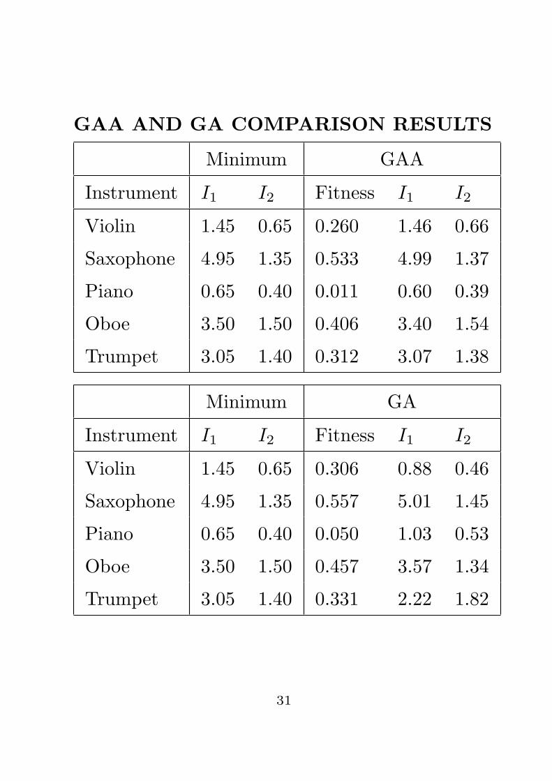
GAA AND GA COMPARISON RESULTS

Minimum GAA

Instrument I1 I2 Fitness I1 I2

Violin 1.45 0.65 0.260 1.46 0.66

Saxophone 4.95 1.35 0.533 4.99 1.37

Piano 0.65 0.40 0.011 0.60 0.39

Oboe 3.50 1.50 0.406 3.40 1.54

Trumpet 3.05 1.40 0.312 3.07 1.38

Minimum GA

Instrument I1 I2 Fitness I1 I2

Violin 1.45 0.65 0.306 0.88 0.46

Saxophone 4.95 1.35 0.557 5.01 1.45

Piano 0.65 0.40 0.050 1.03 0.53

Oboe 3.50 1.50 0.457 3.57 1.34

Trumpet 3.05 1.40 0.331 2.22 1.82

31

TWO OPERATOR DFM

We define one DFM operator as:

x(t) = A sin[I1 sin(ω1t) + I2 sin(ω2t)]

One or more DFM operators may be used tosynthesize an instrument.

For two DFM operators, A and B, we may weightthe operators accordingly with the weights WA

and WB before adding the two operators togetherto obtain the resultant waveform X(t):

X(t) = WA sin[I1A sin(ω1A) + I2A sin(ω2A)]

+ WB sin[I1B sin(ω1B) + I2B sin(ω2B)]

This can be extended to three or more DFMoperators.

32

DFM OPERATOR A AmpA = 0.648809 IndexA1 = 2.605 FreqA1 = 660 Hz IndexA2 = 0.097 FreqA2 = 880 Hz

DFM OPERATOR B AmpB = 1.849750 IndexB1 = 1.437 FreqB1 = 440 Hz IndexB2 = 0.037 FreqB2 = 220 Hz

0

0.2

0.4

0.6

0.8

1

1

fitness = 0.047810

2 3 4 5 6 7 8 9 10 11 12 13 14

Harmonic Frequency ( x 220 Hz )

Classical Oboe

MUMS Sample

Genetic Algorithm

Classical Oboe. DFM parameters estimated by the genetic algorithm.



0

0.2

0.4

0.6

0.8

1

1 2 3 4 5 6 7 8 9 10 11 12 13 14


Classical Oboe

MUMS Sample

Genetic Annealing Algorithm

fitness = 0.018030

Classical Oboe. DFM parameters estimated by the genetic annealing algorithm.

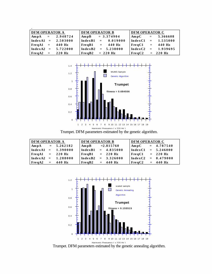
. DFM OPERATOR A AmpA = 2.948724 IndexA1 = 2.503000 FreqA1 = 440 Hz IndexA2 = 5.722000 FreqA2 = 220 Hz


DFM OPERATOR C AmpC = 5.366608 IndexC1 = 1.535000 FreqC1 = 440 Hz IndexC2 = 1.939695 FreqC2 = 220 Hz

0

0.2

0.4

0.6

0.8

1

1.2

1.4

fitness = 0.684556

1 2 3 4 5 6 7 8 9 10 11 12 13 14 15 16 17 18 19


Trumpet

MUMS Sample

Genetic Algorithm

Trumpet. DFM parameters estimated by the genetic algorithm.


DFM OPERATOR B AmpB =2.815760 IndexB1 = 4.835000 FreqB1 = 220 Hz IndexB2 = 3.326000 FreqB2 = 440 Hz

DFM OPERATOR C AmpC = 4.787540 IndexC1 = 5.246000 FreqC1 = 220 Hz IndexC2 = 0.479000 FreqC2 = 440 Hz

0

0.2

0.4

0.6

0.8

1

1.2

fitness = 0.155515

1 2 3 4 5 6 7 8 9 10 11 12 13 14 15 16 17 18 19


Trumpet

scaled sample

Genetic Annealing

Algorithm

Trumpet. DFM parameters estimated by the genetic annealing algorithm.

COMPARISON OF TWO OPERATORFM, AFM AND DFM

Though Yamaha’s famous DX7 synthesizer isdescribed as using 6 operator FM synthesis, onecarrier and one modulating waveform are countedby Yamaha as 2 operators, hence it is 3 operatorsynthesis in our terminology.

Using GAA to optimize 2 operator FM, AFM andDFM synthesis for a number of instruments gavethe following results:

Instrument FM AFM DFM

Trumpet 0.001426 0.000935 0.000658

Saxophone 0.001061 0.000831 0.000280

Oboe 0.001894 0.000887 0.001904

Piano 0.000440 0.000112 0.000088

Violin 0.003970 0.005517 0.002895

Cornet 0.003980 0.002886 0.004440

33

DYNAMIC SYNTHESIS ANDRECYCLING

In order to synthesize dynamic sounds, Each setof optimum parameters for a time frame isrecycled as the initial set of parameters for therecruitment phase for the next time frame. As thespectrum does not vary much from the last timeframe, this enables the next time frame to startwith a set of near-optimized parameters.

This enables the dynamic sound spectrum to besynthesized very efficiently.

As the GAA process is very fast, typically about7 seconds for the initial time frame and about 2seconds for each subsequent time frame, it isconceivable that with faster computers thesynthesis process could proceed in real time.

DFM could then be used as a highly efficientmethod of data compression for the storage andtransmission of the synthesized waveform, as onlythe DFM parameters need be stored ortransmitted.

34

TREE EVOLUTION ALGORITHM

We have proposed a new algorithm named TreeEvolution Algorithm (TEA) based on GAA,which searches the solution space morethoroughly than GAA.

• TEA searches each local minimum separatelyby splitting the population into several parts.

• Each part forms a new population called aspecies and evolves in isolation by focusing onthe closest local minimum through aGAA-like process independently.

• The parents for each GAA crossover arechosen only from the same group ofindividual, analogous to nature in that onlyorganisms of the same species can mate.

• The crossover process of GAA is modified inorder to restrict the offspring to the samespecies as their parents.

• The overall best local solution is selected.

35

VIBRATO IN STRING INSTRUMENTS

Musical instruments may have an oscillation oftheir amplitude and frequency known as vibratowhich is part of the performer’s techniqueimposed on the basic tone of the instrument.

We have initiated a study of the phenomenon ofvibrato in the violin and other string instruments.

We have obtained the Time-Varying Spectrum(TVS) of the dynamic violin tone by employingan 2048 point FFT to extract the peaks of theharmonics of the dynamic tone.

Because of the vibrato, each peak was broaderthan for a tone without vibrato. By assumingthat the energy under each peak is approximatelyconstant, and that the actual spectrum consists oftime-varying delta peaks, we can obtain theequivalent amplitude of each delta peak.

36

TIME VARYING SPECTRUM (TVS)

The TVS of a tone can be split into 2 parts:

• The Time Varying Amplitude (TVA),the variation of the amplitude.

• The Time Varying Frequency (TVF), thevariation of the frequency.

The TVA in turn can be split with a low-passfilter into:

• The Time Varying Principal Amplitude(TVPA), which is the non-vibrato part ofthe amplitude variation.

• The Time Varying AmplitudeModulation (TVAM), which is due to thevibrato.

Likewise the TVF can be split into:

• The Time Varying Principal Frequency(TVPF).

• The Time Varying FrequencyModulation (TVFM).

37

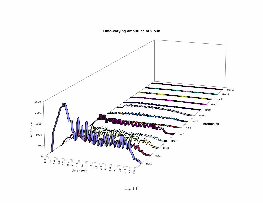
Fig. 1.1

0.0

0.2

0.4

0.6

0.7

0.9

1.1

1.3

1.5

1.7

1.9

2.0

2.2

2.4

2.6

2.8

3.0

3.2

3.3

3.5

Har1

Har2

Har3

Har4

Har5

Har6

Har7

Har8

Har9

Har10

Har11

Har12

Har13

0

500

1000

1500

2000

2500

ampl

itude

time (sec)

harmonics

Time-Varying Amplitude of Violin

Fig. 1.2

0.0

0.2

0.4

0.6

0.8

1.0

1.2

1.3

1.5

1.7

1.9

2.1

2.3

2.5

2.6

2.8

3.0

3.2

3.4

3.6

Har1

Har2

Har3

Har4

Har5

Har6

Har7

Har8

Har9

Har10

Har11

Har12

Har13

410

415

420

425

430

435

440

445

450

455

460

freq

uenc

y (H

z)

time (sec)

harmonics

Time-Varying Frequency of Violin

Fig. 7.1

0.0

0.2

0.4

0.6

0.7

0.9

1.1

1.3

1.5

1.7

1.9

2.0

2.2

2.4

2.6

2.8

3.0

3.2

3.3

3.5

Har1

Har2

Har3

Har4

Har5

Har6

Har7

Har8

Har9

Har10

Har11

Har12

Har13

0

500

1000

1500

2000

2500

ampl

itude

time (sec)

harmonics

Time-Varying Principal Amplitude of Violin

Fig. 7.2

0.0

0.2

0.4

0.6

0.7

0.9

1.1

1.3

1.5

1.7

1.9

2.0

2.2

2.4

2.6

2.8

3.0

3.2

3.3

3.5

Har1

Har2

Har3

Har4

Har5

Har6

Har7

Har8

Har9

Har10

Har11

Har12

Har13

-600

-400

-200

0

200

400

600

800

ampl

itude

mod

ulat

ion

time (sec)

harmonics

Amplitude Modulation of Violin

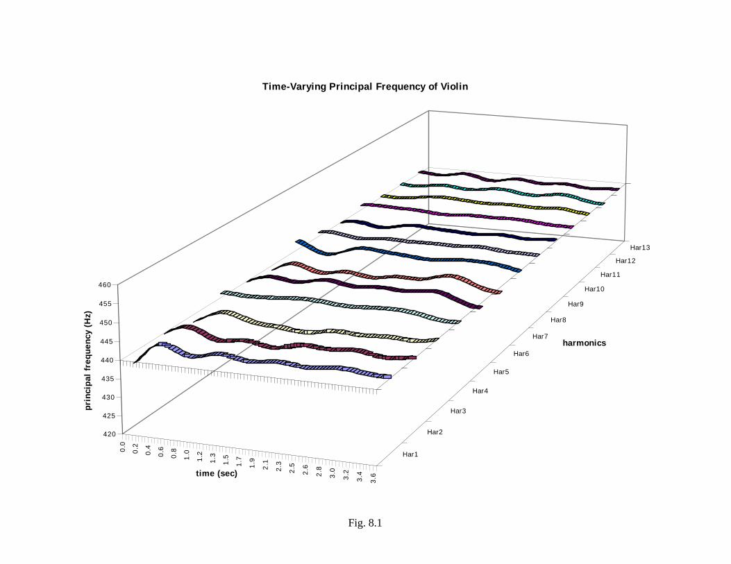
Fig. 8.1

0.0

0.2

0.4

0.6

0.8

1.0

1.2

1.3

1.5

1.7

1.9

2.1

2.3

2.5

2.6

2.8

3.0

3.2

3.4

3.6

Har1

Har2

Har3

Har4

Har5

Har6

Har7

Har8

Har9

Har10

Har11

Har12

Har13

420

425

430

435

440

445

450

455

460

prin

cipa

l fre

quen

cy (H

z)

time (sec)

harmonics

Time-Varying Principal Frequency of Violin

Fig. 8.2

0.0

0.2

0.4

0.6

0.8

1.0

1.2

1.3

1.5

1.7

1.9

2.1

2.3

2.5

2.6

2.8

3.0

3.2

3.4

3.6

Har1

Har2

Har3

Har4

Har5

Har6

Har7

Har8

Har9

Har10

Har11

Har12

Har13

-20

-15

-10

-5

0

5

10

15

20

freq

uenc

y m

odua

ltion

(Hz)

time (sec)

harmonics

Time-Varying Frequency Modulation of Violin

ADDITIVE SYNTHESIS OF VIBRATO

We have

TVS = TVA + TVF whereTVA = TVPA + TVAM andTVF = TVPF + TVFM.

We have chosen to use such an additive model forthe vibrato because the information extractedthrough the filter is additive and such a modelprovides great flexibility in analysis and simplicityin the real time synthesis of the vibrato.

The maximum average excursion of the for theviolin and the other string instruments analyzedis about 3.4Hz to 4.0Hz for A=440 HGz, and themajor vibrato rate is about 5.5Hz to 5.9Hz.

We synthesized a vibrato tone by adding thesynthesized principal spectrum and thesynthesized modulation spectrum. Thesynthesized vibrato tone was very close to theoriginal real violin tone with vibrato.

BT/26.04.2001

38

musical soundsdigital synthesis of

Documents