musculoskeletal model of the human shoulder for joint force
TRANSCRIPT

POUR L'OBTENTION DU GRADE DE DOCTEUR ÈS SCIENCES
acceptée sur proposition du jury:
Dr A. Karimi, président du juryProf. R. Longchamp, Dr Ph. Müllhaupt, directeurs de thèse
Prof. R. Dumas, rapporteur Prof. J. Rasmussen, rapporteur
Dr A. Terrier, rapporteur
Musculoskeletal Model of the Human Shoulder for Joint Force Estimation
THÈSE NO 6497 (2015)
ÉCOLE POLYTECHNIQUE FÉDÉRALE DE LAUSANNE
PRÉSENTÉE LE 30 JANVIER 2015
À LA FACULTÉ DES SCIENCES ET TECHNIQUES DE L'INGÉNIEURLABORATOIRE D'AUTOMATIQUE - COMMUN
PROGRAMME DOCTORAL EN SYSTÈMES DE PRODUCTION ET ROBOTIQUE
Suisse2015
PAR
David INGRAM

ii

The wheels on the bus goround and round...
— Unknown
To my son Jonathan and my father Jim.


Acknowledgements
Writing a PhD dissertation is a voyage through the zone where normal things don’t hap-pen very often. Its a long personal journey that ends with a great uproar. However, thejourney would not be possible without the help and support of so many others. I wouldtherefore like to take this opportunity to express my thanks towards everyone who madethis work possible.
First, I express my gratitude to my thesis directors, Prof. Roland Longchamp and Dr.Philippe Mullhaupt, without whom nothing would have been possible. The interactionswith Dr. Mullhaupt kept my work focused and provided feedback for improvements. Iwould like to thank the external members of the jury, Prof. John Rasmussen and Prof.Raphael Dumas for their insight and constructive criticism. I would like to thank Dr.Alexandre Terrier for his participation in my research and for his presence on my jury. Ialso thank Dr. Alireza Karimi, the jury president. I thank Ehsan Sarshari for continuingmy work and Christoph Engelhardt for overseeing the other side of things. The financialsupport from the Swiss National Science Foundation is gratefully acknowledged.
The Laboratoire d’Automatique provides a great atmosphere for work and for fun.As a great philosopher once said: ”work before play”. I would therefore like to thank themembers of the lab direction for having granted me the possibility of caring out a PhD. Iwould also like to thank those who facilitated administrative tasks. Ruth for making sureeverything went smoothly. Francine for helping with the travel planning and financialtasks. As well as Petiote and Eva for making sure we pay our cafeteria fees on time. In noparticular order, I want to thank all those who made my PhD a memorable experience;Philippe, for having aided in the creation of ”Bouinopia”, the capitol city of crazy ideasand wacky concepts. You are also the permanent boss of the ”Empty Head ResearchGroup” where people can study hyperlinearism and control evitciderp del futuro. San-dra, for her friendship and being a good colleague; Francine ”La Migrue”, for alwayskeeping me focused on the important things in life. Francis for helping me test some ofmy more fundamental research ideas like: how to homogeneously roast a marshmallow.Dr. Christoph ”Neo” Salzmann for your precious help with experiments; Dr. Gillet forbeing my mentor; Basile for being a really good office partner and a good friend, alwaysready for a good laugh. Willson for his friendship and help in putting my PhD on theright track from the start. Gorka for proving that Nutela is a food group. Andrijanafor creating the LA nail salon and her friendship. Evgeny for showing me how to cross-country ski properly. Timm for sharing my passion for downhill mountain biking. Seanfor being Irish and a good friend and colleague. Greg; Jean-Hubert; Sriniketh. Thankyou to all my other lab colleagues.
i
ii Acknowledgements
A lot of thanks goes to all friends in and around Lausanne as well as elsewhere. Youalways provided great moments.
I would like to thank my parents. Thanks to your love and support, I have had thegreat opportunity of doing a doctoral dissertation. Thanks also to my brothers, James,Michael and John.I would like to thank my wife Sandy for all the love and support. It definitely was noteasy, but you got me through the smooth and the rough times. You always knew whatto say to keep me motivated. Thank you for making me who I am today.Finally, I would like to thank my son Jonathan. Without your smiles and laughs, thefinal moments would not have been as enjoyable. This thesis is dedicated to you and toyour grandfather.
Lausanne, 12 Janvier 2015 D. I.

Abstract
Human beings like all organisms, are subject to a variety of diseases. Musculoskeletaldiseases such as arthritis, affecting our muscles and bones, are particularly debilitatingbecause they considerably limit our ability to interact with our environment. The symp-toms of arthritis are joint pain and loss of movement, caused by a deterioration of thecartilage in our articulations. The precise determination of the underlying cause of thedeterioration is a challenging task. It is believed that it is caused by excessive force inthe joints due to inappropriate muscle forces. Since only forces in muscles just beneaththe skin can be measured, the force hypothesis remains unproven. Musculoskeletal mod-els are essential in analysing musculoskeletal diseases because they address the lack ofinformation on the forces involved. Such models are used to estimate muscle and jointreaction forces. Determining the key elements in a musculoskeletal model to assess itsquality raises several challenges.
In this thesis, a musculoskeletal model of the shoulder is presented. The model isgoverned by the laws of rigid-body mechanics and is similar to a model of a cable-drivenmechanism. Both the kinematic and dynamic aspects of the shoulder are contained inthe model. Applying the theory of rigid body mechanics requires a certain level of rigourto ensure compatibility between the kinematic and dynamic parts of the model. There-fore, a considerable part of the thesis is devoted to presenting the details of the model’sconstruction. The model is designed specifically for estimating muscle and joint-reactionforces in quasi-static and dynamic situations.
The muscle-force estimation problem is defined as a nonlinear program and solved inthis thesis using a two-step approach. In a first step, the desired kinematics is constructedand inverse dynamics is used to estimate the associated joint torques. In a second step,the nonlinear program is solved using null-space optimisation. An initial solution to theestimation problem is obtained by taking a pseudo-inverse of the moment-arms matrix.The solution is then corrected using the matrix’s null-space to satisfy the constraints.This approach redefines the estimation problem as a quadratic program and considerablyreduces the time required to find a solution. Once the muscle-forces are estimated, thejoint reaction forces are deduced from the dynamic model. Muscle and joint-reactionforces are compared to other results from the literature.
A key element of the first step is building the kinematics. The model’s kinematicsare analysed and a new method for describing them is presented. Indeed, obtaining com-patible motion for the model’s dynamics is a challenging task. The inverse kinematicstechnique is inappropriate and measured joint angle data is not always available. The
iii

iv Acknowledgements
shoulder girdle is shown to be a parallel platform with three degrees of freedom. Thekinematics are described by three coordinates obtained from a geometric interpretationof the scapulothoracic contact. The coordinates provide a direct, efficient method ofplanning the shoulder’s motion, directly compatible with the dynamic model.
A key element of solving the nonlinear program, second step of the muscle-force es-timation problem, is computing muscle moment-arms. A rigorous definition of musclemoment-arms is presented. The definition provides an alternative to the tendon excur-sion method that can lead to incorrect moment-arms if used inappropriately due to itsdependency on the choice of joint coordinates. The proposed definition is independent ofany kinematic coordinate choice. It is used to analyse the problem of the existence of asolution through the wrench- and torque-feasible sets. An analysis of the torque-feasibleset is used to answer certain questions regarding the underestimation of certain muscleactivities.
Lastly, the problem of how musculoskeletal systems are controlled through antagonis-tic muscle structures is addressed. A hypothesis for the cause of arthritis is a deteriorationof neuromuscular coordination. Muscles are being badly coordinated by the neurologicalsystem. Given the similarities between musculoskeletal models and cable-driven systems,the problem is analysed using a cable-driven pendulum. The pendulum model consti-tutes a simplified model of the shoulder and is used to prove the stability of a humanmotor control mechanism called joint stiffness control through antagonistic muscle co-contraction. A control strategy is developed for the pendulum based on the mechanismof muscle co-contraction. Given a joint stiffness, the necessary muscle forces are obtainedusing the estimation method previously described. The strategy is applied to a physicalcable-driven pendulum. Four cables, each controlled independently through a motor-driven pulley, drive the pendulum. The results are used to open the discussion on thepossible neurological causes of neuromuscular dysfunctions.
Keywords: musculoskeletal modelling, shoulder mechanics, muscle-force estimation,joint-force estimation, moment-arms, cable-driven systems.

Version abregee
Les etres humains, comme tous les organismes vivants, sont exposes a une variete demaladies. Les maladies musculo-squelettiques comme l’arthrose, lequel affectent les mus-cles et les os, limitent considerablement notre capacite d’interagir avec notre environ-nement. Des douleurs articulaires et une perte de mouvement constituent les princi-paux symptomes de l’arthrose. Il s’agit d’une degradation du cartilage articulaire. Ladetermination precise de la cause sous-jacente de la degradation est une tache difficile.On croit que cette degradation est causee par une force excessive dans les articulations,en raison de l’application de forces musculaires inappropriees. Etant donne que seulesles forces musculaires sous la peau peuvent etre mesurees, l’hypothese de la force restea prouver. Les modeles musculo-squelettiques sont essentiels dans l’analyse de l’arthroseparce qu’ils fournissent des informations manquantes relatives aux forces impliquees.Ces modeles sont utilises pour estimer les forces musculaires et les forces articulaires.La determination des elements cles d’un modele musculo-squelettique, afin d’evaluer saqualite, souleve plusieurs defis.
Dans cette these, un modele musculo-squelettique de l’epaule est presente. Le modeleest regi par les lois de la mecanique des corps rigides, et elle est similaire a un modeled’un mecanisme actionne par cables. Le modele contient les deux aspects, cinematiqueset dynamiques, de l’epaule. L’application de la theorie de la mecanique des corps rigidesnecessite un certain niveau de rigueur pour assurer la compatibilite entre les partiescinematiques et dynamiques du modele. Par consequent, une grande partie de la theseest consacree a la presentation des details de la construction du modele. Le modele estspecifiquement concu pour estimer les forces musculaires et articulaires, dans des situa-tions quasi - statiques et dynamiques.
L’estimation des forces musculaires est definie comme un programme non lineaire etresolue dans cette these en utilisant une approche en deux etapes. Dans une premiereetape, le modele cinematique est construit, et la dynamique inverse est utilisee pour es-timer les couples articulaires associes au mouvement de l’epaule. Dans une deuxiemeetape, le programme non lineaire est resolu en utilisant l’optimisation du nul espace.Une premiere solution au probleme d’estimation est obtenue en prenant un pseudo-inverse de la matrice des bras de levier. La solution est ensuite corrigee en utilisantle nul espace de la matrice afin de satisfaire les contraintes. Cette approche redefinitle probleme d’estimation comme un programme quadratique et reduit considerablementle temps necessaire pour trouver une solution. Une fois que les forces musculaires sontestimees, les forces articulaires sont deduites a partir du modele dynamique. Les forcesmusculaires et articulaires estimees sont comparees a d’autres resultats de la litterature.
v

vi Acknowledgements
Un element cle de la premiere etape est la construction de la cinematique. Lacinematique du modele est analysee et une nouvelle methode pour les decrire est presentee.En effet, l’obtention de mouvement compatible pour la dynamique du modele est unetache laborieuse. La technique de cinematique inverse est inappropriee et les donneesdes angles articulaires mesures n’est pas toujours disponible. La ceinture scapulaire estindiquee comme etant une plate-forme parallele a trois degres de liberte. La cinematiqueest decrites par trois coordonnees obtenues a partir d’une interpretation geometrique ducontact scapulo-thoracique. Les coordonnees constituent une methode efficace de plan-ification directe du mouvement de l’epaule, lequel est directement compatible avec lemodele dynamique de l’epaule.
Un element cle de la resolution du programme non-lineaire, deuxieme etape du problemed’estimation des forces musculaires, est le calcul des bras de levier musculaires. Unedefinition rigoureuse des bras de levier musculaires est presentee. La definition offre unealternative a la methode d’excursion du tendon, laquelle pourrait induire des erreurs dansles bras de levier si utilisee de facon inappropriee, en raison de sa dependance du choixdes coordonnees des articulations. La definition proposee est independante de tout choixde coordonnees cinematique. Elle est utilisee afin d’analyser le probleme de l’existenced’une solution a travers les espaces de realisation cinematique et de couples. Une analysede l’espace de couple realisable est utilisee pour repondre a certaines questions concernantla sous-estimation de l’activite de certains muscles.
Pour finir, le controle des systemes musculo-squelettique par des structures muscu-laires antagonistes est adressee. Une hypothese expliquant l’origine de l’arthrose est unedeterioration de la coordination neuro-musculaire. Les muscles sont mal coordonnes par lesysteme neurologique. Etant donne les similarites entre les modeles musculo-squelettiqueset les systemes actionnes par cables, le probleme est analysee a travers un pendule ac-tionne par cables. Le pendule constitue un modele simplifie de l’epaule et est utilise pourprouver la stabilite d’un mecanisme de controle humain appele le controle de la raideurarticulaire par co-contraction des muscles antagonistes. Une strategie de controle est pro-posee, basee sur la co-contraction musculaires. Etant donne une raideur articulaire, lesforces musculaires necessaire sont obtenue en utilisant la methode d’estimation decriteprecedemment. La strategie de controle est appliquee a un pendule physique. Quatrecables, chacun controlee de maniere independante a travers des moteurs et poulies, ac-tionnent le pendule. Les resultats sont utilises pour ouvrir la discussion sur les causespossibles d’une deterioration de la coordination neuro-musculaire.
Mots-cles: modelisation musculo-squelettique, mecanique de l’epaule, estimation deforces musculaires, estimation de forces articulaires, bras de levier, systemes actionnespar cables.

Contents
Acknowledgements i
List of figures xi
List of tables xv
List of Symbols xvii
1 Introduction 1
1.1 Research Context . . . . . . . . . . . . . . . . . . . . . . . . . . . . . . . 11.2 State of the Art . . . . . . . . . . . . . . . . . . . . . . . . . . . . . . . . 31.3 Contributions . . . . . . . . . . . . . . . . . . . . . . . . . . . . . . . . . 61.4 Organisation of the Thesis . . . . . . . . . . . . . . . . . . . . . . . . . . 8
2 Anatomy, Physiology and Movement of the Human Shoulder 11
2.1 Shoulder Skeletal Anatomy and Physiology . . . . . . . . . . . . . . . . . 112.2 Shoulder Muscle Anatomy and Physiology . . . . . . . . . . . . . . . . . 142.3 Shoulder Movement . . . . . . . . . . . . . . . . . . . . . . . . . . . . . . 16
3 Multibody Systems Theory 21
3.1 Introduction . . . . . . . . . . . . . . . . . . . . . . . . . . . . . . . . . . 213.2 Preliminaries . . . . . . . . . . . . . . . . . . . . . . . . . . . . . . . . . 22
3.2.1 Conventions . . . . . . . . . . . . . . . . . . . . . . . . . . . . . . 223.2.2 Geometric Configuration . . . . . . . . . . . . . . . . . . . . . . . 233.2.3 Euclidean Displacements . . . . . . . . . . . . . . . . . . . . . . . 243.2.4 Rotation Matrices . . . . . . . . . . . . . . . . . . . . . . . . . . . 263.2.5 Angular Description of Rotations . . . . . . . . . . . . . . . . . . 273.2.6 Euler’s Rotation Theorem . . . . . . . . . . . . . . . . . . . . . . 29
3.3 Rigid-Body Kinematics . . . . . . . . . . . . . . . . . . . . . . . . . . . . 303.3.1 Instantaneous Angular velocity . . . . . . . . . . . . . . . . . . . 303.3.2 Instantaneous Kinematics . . . . . . . . . . . . . . . . . . . . . . 323.3.3 Movement: Velocity and Acceleration . . . . . . . . . . . . . . . . 333.3.4 Chasles’ Theorem and the Instantaneous Screw Axis . . . . . . . 35
3.4 Rigid-Body Dynamics . . . . . . . . . . . . . . . . . . . . . . . . . . . . 383.4.1 Newtonian Mechanics . . . . . . . . . . . . . . . . . . . . . . . . . 383.4.2 Forces, Moments of Force and Poinsot’s Theorem . . . . . . . . . 393.4.3 Inertia and Moment of Inertia . . . . . . . . . . . . . . . . . . . . 43
vii

viii CONTENTS
3.4.4 Equations of Motion . . . . . . . . . . . . . . . . . . . . . . . . . 443.4.5 Mechanical Energy, Work and Power . . . . . . . . . . . . . . . . 48
3.5 Multibody Kinematics . . . . . . . . . . . . . . . . . . . . . . . . . . . . 523.5.1 Machines and Mechanisms . . . . . . . . . . . . . . . . . . . . . . 523.5.2 Kinematic Pairs and Kinematic Chains . . . . . . . . . . . . . . . 533.5.3 Forward Kinematics and Mobility . . . . . . . . . . . . . . . . . . 573.5.4 Kinematic Constraints . . . . . . . . . . . . . . . . . . . . . . . . 603.5.5 Forward Kinematic Map . . . . . . . . . . . . . . . . . . . . . . . 61
3.6 Multibody dynamics . . . . . . . . . . . . . . . . . . . . . . . . . . . . . 623.6.1 Analytical Mechanics and Virtual Displacements . . . . . . . . . . 623.6.2 The Principles of Jourdain and d’Alembert . . . . . . . . . . . . . 653.6.3 Principle of Virtual Power . . . . . . . . . . . . . . . . . . . . . . 663.6.4 The Euler-Lagrange Equation . . . . . . . . . . . . . . . . . . . . 673.6.5 The Principle of Virtual Work and Static Equilibrium . . . . . . . 71
4 A Musculoskeletal Model of the Human Shoulder 73
4.1 Introduction . . . . . . . . . . . . . . . . . . . . . . . . . . . . . . . . . . 734.2 Kinematic Shoulder Model . . . . . . . . . . . . . . . . . . . . . . . . . . 74
4.2.1 Bony Landmarks and Reference Frames . . . . . . . . . . . . . . . 754.2.2 Joint Angle Parameterisation of the Model’s Kinematics . . . . . 774.2.3 Scapulothoracic Contact Model . . . . . . . . . . . . . . . . . . . 794.2.4 Forward Kinematic Map . . . . . . . . . . . . . . . . . . . . . . . 81
4.3 Dynamic Shoulder Model . . . . . . . . . . . . . . . . . . . . . . . . . . . 824.3.1 Equations of Motion . . . . . . . . . . . . . . . . . . . . . . . . . 824.3.2 Muscle Forces . . . . . . . . . . . . . . . . . . . . . . . . . . . . . 854.3.3 Muscle Cable Model . . . . . . . . . . . . . . . . . . . . . . . . . 87
4.4 Remarks . . . . . . . . . . . . . . . . . . . . . . . . . . . . . . . . . . . . 894.5 Conclusions . . . . . . . . . . . . . . . . . . . . . . . . . . . . . . . . . . 91
5 Coordinated Redundancy 93
5.1 Introduction . . . . . . . . . . . . . . . . . . . . . . . . . . . . . . . . . . 935.2 Kinematic Redundancy . . . . . . . . . . . . . . . . . . . . . . . . . . . . 945.3 Overactuation . . . . . . . . . . . . . . . . . . . . . . . . . . . . . . . . . 975.4 Tasks for Coordination Strategies . . . . . . . . . . . . . . . . . . . . . . 98
6 Shoulder Kinematic Redundancy Coordination 103
6.1 Introduction . . . . . . . . . . . . . . . . . . . . . . . . . . . . . . . . . . 1036.2 Minimal Coordinates for Coordination . . . . . . . . . . . . . . . . . . . 105
6.2.1 Shoulder Kinematic Redundancy Coordination . . . . . . . . . . . 1056.2.2 Manifolds and Coordinate Reduction . . . . . . . . . . . . . . . . 1086.2.3 A Parallel Platform Kinematic Shoulder Model . . . . . . . . . . 1146.2.4 Equivalent Kinematic Maps and Coordinates . . . . . . . . . . . . 1176.2.5 The Coordinate Space . . . . . . . . . . . . . . . . . . . . . . . . 1226.2.6 A Minimal Parameterisation . . . . . . . . . . . . . . . . . . . . . 124
6.3 Remarks . . . . . . . . . . . . . . . . . . . . . . . . . . . . . . . . . . . . 1306.3.1 Trammel of Archimedes . . . . . . . . . . . . . . . . . . . . . . . 131

CONTENTS ix
6.4 Conclusions . . . . . . . . . . . . . . . . . . . . . . . . . . . . . . . . . . 133
7 Shoulder Overactuation Coordination 135
7.1 Introduction . . . . . . . . . . . . . . . . . . . . . . . . . . . . . . . . . . 1357.2 Moment-Arms for Coordination . . . . . . . . . . . . . . . . . . . . . . . 137
7.2.1 Shoulder Overactuation Coordination . . . . . . . . . . . . . . . . 1377.2.2 Constraint Gradient Projection . . . . . . . . . . . . . . . . . . . 1397.2.3 A Coordination Strategy to Shoulder Overactuation . . . . . . . . 142
7.3 Muscle Moment-Arms Theory . . . . . . . . . . . . . . . . . . . . . . . . 1457.3.1 Fundamentals of Moment-Arms . . . . . . . . . . . . . . . . . . . 1467.3.2 A Geometric Method of Computing Moment-Arms . . . . . . . . 1477.3.3 Tendon Excursion Method of Computing Moment-Arms . . . . . 1517.3.4 Computing Muscle Moment-Arms . . . . . . . . . . . . . . . . . . 153
7.4 The Solution Set and Wrench-Feasibility . . . . . . . . . . . . . . . . . . 1557.5 Conclusions . . . . . . . . . . . . . . . . . . . . . . . . . . . . . . . . . . 159
8 Estimating Joint Force in the Human Shoulder 161
8.1 Introduction . . . . . . . . . . . . . . . . . . . . . . . . . . . . . . . . . . 1618.2 Methods . . . . . . . . . . . . . . . . . . . . . . . . . . . . . . . . . . . . 162
8.2.1 A Musculoskeletal Model of the Human Shoulder . . . . . . . . . 1628.2.2 Kinematic Coordination . . . . . . . . . . . . . . . . . . . . . . . 1658.2.3 Muscle-Force Coordination . . . . . . . . . . . . . . . . . . . . . . 1688.2.4 Implementation and Model Output . . . . . . . . . . . . . . . . . 169
8.3 Results . . . . . . . . . . . . . . . . . . . . . . . . . . . . . . . . . . . . . 1728.3.1 Scapular Kinematics . . . . . . . . . . . . . . . . . . . . . . . . . 1728.3.2 Muscle Moment-Arms . . . . . . . . . . . . . . . . . . . . . . . . 1728.3.3 Muscle Forces . . . . . . . . . . . . . . . . . . . . . . . . . . . . . 1748.3.4 Joint Reaction Force . . . . . . . . . . . . . . . . . . . . . . . . . 176
8.4 Discussion . . . . . . . . . . . . . . . . . . . . . . . . . . . . . . . . . . . 1778.4.1 Wrench-Feasibility of a Shoulder Musculoskeletal Model . . . . . . 179
8.5 Conclusions . . . . . . . . . . . . . . . . . . . . . . . . . . . . . . . . . . 185
9 Introduction to Control Theory 187
9.1 Systems and Controllers . . . . . . . . . . . . . . . . . . . . . . . . . . . 1879.2 Open-Loop and Closed-Loop . . . . . . . . . . . . . . . . . . . . . . . . . 1899.3 Stability . . . . . . . . . . . . . . . . . . . . . . . . . . . . . . . . . . . . 1919.4 Linear State Feedback Control . . . . . . . . . . . . . . . . . . . . . . . . 195
10 Musculoskeletal Stability through Joint Stiffness Control 199
10.1 Introduction . . . . . . . . . . . . . . . . . . . . . . . . . . . . . . . . . . 19910.2 Stability by Antagonistic Muscle Co-contraction . . . . . . . . . . . . . . 201
10.2.1 Human Motor Control . . . . . . . . . . . . . . . . . . . . . . . . 20110.2.2 Stability in Human Motor Control . . . . . . . . . . . . . . . . . 20410.2.3 Model of a Cable-Driven Pendulum . . . . . . . . . . . . . . . . . 20610.2.4 Stability by Antagonistic Cable Co-contraction . . . . . . . . . . . 21010.2.5 Joint Stiffness Control . . . . . . . . . . . . . . . . . . . . . . . . 21310.2.6 Observability of Pendulum States . . . . . . . . . . . . . . . . . . 215

x CONTENTS
10.3 A Joint Stiffness Control Strategy . . . . . . . . . . . . . . . . . . . . . . 21710.3.1 Control Algorithm . . . . . . . . . . . . . . . . . . . . . . . . . . 21810.3.2 Implementation . . . . . . . . . . . . . . . . . . . . . . . . . . . . 22110.3.3 Methods . . . . . . . . . . . . . . . . . . . . . . . . . . . . . . . . 224
10.4 Results . . . . . . . . . . . . . . . . . . . . . . . . . . . . . . . . . . . . . 22510.5 Discussion . . . . . . . . . . . . . . . . . . . . . . . . . . . . . . . . . . . 22610.6 Conclusions . . . . . . . . . . . . . . . . . . . . . . . . . . . . . . . . . . 229
11 Conclusions 231
11.1 Contributions . . . . . . . . . . . . . . . . . . . . . . . . . . . . . . . . . 23211.2 Future Research Directions . . . . . . . . . . . . . . . . . . . . . . . . . . 234
A Technical Details 237
A.1 Uniform Dilation of an Ellipsoid . . . . . . . . . . . . . . . . . . . . . . . 237A.2 Sphere-Ellipsoid Intersection . . . . . . . . . . . . . . . . . . . . . . . . . 239
A.2.1 Quadric Surfaces . . . . . . . . . . . . . . . . . . . . . . . . . . . 239A.2.2 Ruled Surfaces . . . . . . . . . . . . . . . . . . . . . . . . . . . . 241A.2.3 Quadric-Quadric Intersections . . . . . . . . . . . . . . . . . . . . 243A.2.4 Sphere-Ellipsoid Intersection . . . . . . . . . . . . . . . . . . . . . 244
B Shoulder Model Numerical Dataset 247
B.1 Bony Landmarks and Rotation Matrices . . . . . . . . . . . . . . . . . . 247B.2 Mass, Intertia and Glendoid Stability . . . . . . . . . . . . . . . . . . . . 249B.3 Muscle Geometry and Wrapping . . . . . . . . . . . . . . . . . . . . . . . 250
Glossary 273
Curriculum Vitae 281

List of Figures
1.1 The shoulder’s skeletal structure . . . . . . . . . . . . . . . . . . . . . . . 31.2 The linkage model and joint sinus cones . . . . . . . . . . . . . . . . . . 41.3 Three musculoskeletal shoulder models from the literature . . . . . . . . 5
2.1 The shoulder’s skeletal anatomy . . . . . . . . . . . . . . . . . . . . . . . 122.2 The shoulder’s articulations and ligaments . . . . . . . . . . . . . . . . . 132.3 The glenoid cavity in the glenohumeral joint . . . . . . . . . . . . . . . . 132.4 The shoulder’s muscle structure . . . . . . . . . . . . . . . . . . . . . . . 142.5 Typical force-length behaviour of a skeletal muscle . . . . . . . . . . . . . 162.6 The three body planes and the scapular plane . . . . . . . . . . . . . . . 172.7 Schematic description of shoulder bone motion definitions . . . . . . . . . 182.8 Three phase description of the scapulo-humeral rhythm . . . . . . . . . . 19
3.1 Coordinate system convention . . . . . . . . . . . . . . . . . . . . . . . . 223.2 A free rigid-body’s geometric configuration . . . . . . . . . . . . . . . . . 233.3 A Euclidean displacement . . . . . . . . . . . . . . . . . . . . . . . . . . 253.4 A coordinate transformation . . . . . . . . . . . . . . . . . . . . . . . . . 253.5 Euler and Bryan angle rotation sequences . . . . . . . . . . . . . . . . . . 283.6 Illustration of Euler’s Theorem . . . . . . . . . . . . . . . . . . . . . . . 303.7 A screw encoding a helical vector field . . . . . . . . . . . . . . . . . . . 363.8 Construction of the instantaneous screw axis . . . . . . . . . . . . . . . . 373.9 The moment of force created by a force . . . . . . . . . . . . . . . . . . . 403.10 Duality between Chasles’ theorem and Poinsot’s theorem . . . . . . . . . 423.11 A rigid body as a collection of particles or a continuous mass distribution 443.12 Construction of the dynamics of a rigid body . . . . . . . . . . . . . . . . 463.13 A body moving along a path . . . . . . . . . . . . . . . . . . . . . . . . . 483.14 Illustration of the energy conservation theorem . . . . . . . . . . . . . . . 503.15 Machines and their corresponding mechanisms . . . . . . . . . . . . . . . 533.16 The six lower kinematic pairs with their symbology . . . . . . . . . . . . 543.17 The higher kinematic pairs with their symbology . . . . . . . . . . . . . . 553.18 Kinematic relation between two bodies in a kinematic pair . . . . . . . . 563.19 Displacement of a kinematic pair in a mechanism . . . . . . . . . . . . . 59
4.1 The shoulder’s bony landmarks . . . . . . . . . . . . . . . . . . . . . . . 764.2 Joint coordinates and reference systems . . . . . . . . . . . . . . . . . . . 784.3 Scapulothoracic contact model . . . . . . . . . . . . . . . . . . . . . . . . 804.4 The shoulder mechanism . . . . . . . . . . . . . . . . . . . . . . . . . . . 84
xi

xii LIST OF FIGURES
4.5 Centroid line approach to muscle modelling . . . . . . . . . . . . . . . . . 874.6 3rd order spline parameterisation of muscle segments . . . . . . . . . . . 884.7 The pectoralis major in the model . . . . . . . . . . . . . . . . . . . . . . 89
5.1 Coordinated redundancy in a milling machine . . . . . . . . . . . . . . . 945.2 Machines and their corresponding mechanisms . . . . . . . . . . . . . . . 955.3 Local manifolds in coordinated redundancy . . . . . . . . . . . . . . . . . 99
6.1 Bony landmarks, reference frames and joint coordinates . . . . . . . . . . 1056.2 Diagram of the shoulder’s kinematic model . . . . . . . . . . . . . . . . . 1076.3 Examples of well known two-dimensional compact smooth manifolds . . . 1096.4 Diagram of two charts of a C∞ atlas on a differentiable (smooth) manifold 1106.5 A two-dimensional analogue for the shoulder . . . . . . . . . . . . . . . . 1116.6 Two-dimensional analogue shoulder model with the new kinematic chain 1136.7 Mechanical description of a free body in space . . . . . . . . . . . . . . . 1166.8 Mechanism of a rigid body’s motion on a two-dimensional surface . . . . 1176.9 Equivalent parallel shoulder model . . . . . . . . . . . . . . . . . . . . . 1186.10 Three methods of parameterising the forward kinematic map . . . . . . . 1216.11 Coordinates in the coordinate submanifolds . . . . . . . . . . . . . . . . 1236.12 The natural kinematic map charts . . . . . . . . . . . . . . . . . . . . . . 1246.13 The submanifold decomposition . . . . . . . . . . . . . . . . . . . . . . . 1256.14 Polynomial description of the scapula’s configuration . . . . . . . . . . . 1266.15 The minimal set of coordinates . . . . . . . . . . . . . . . . . . . . . . . 1286.16 The minimal coordinate charts onto the submanifolds . . . . . . . . . . . 1296.17 The driven Trammel of Archimedes . . . . . . . . . . . . . . . . . . . . . 1326.18 A use of the Trammel of Archimedes . . . . . . . . . . . . . . . . . . . . 133
7.1 Bony landmarks, reference frames and joint coordinates . . . . . . . . . . 1387.2 Diagram of a manifold QS in R
3 of dimension 2: the two-torus T 2 . . . . 1407.3 Construction of the GH joint stability constraint . . . . . . . . . . . . . . 1437.4 The classical mechanics definition of force moment-arm . . . . . . . . . . 1467.5 A skeletal system with N joints and two muscles . . . . . . . . . . . . . . 1487.6 Force isolation in moment-arm computations . . . . . . . . . . . . . . . . 1497.7 Force cancellation and force transmission in a musculoskeletal model . . . 1507.8 Inappropriate use of the tendon-excursion method . . . . . . . . . . . . . 1547.9 A two-dimensional toy musculoskeletal model . . . . . . . . . . . . . . . 1577.10 Range and image spaces of the torque-force map . . . . . . . . . . . . . . 1577.11 Image space of the torque-force map in three different configurations . . . 1587.12 The time-dependent behaviour of the image space polytope . . . . . . . . 159
8.1 Bony landmarks, reference frames and joint coordinates . . . . . . . . . . 1638.2 Minimal coordinates used to coordinate the shoulder . . . . . . . . . . . 1668.3 The implemented musculoskeletal shoulder model . . . . . . . . . . . . . 1718.4 Comparison of model-predicted and measured kinematics . . . . . . . . . 1728.5 Comparison of mode-predicted and measured moment-arms . . . . . . . . 1738.6 Muscle forces during abduction in the scapular plane . . . . . . . . . . . 1758.7 Comparions of glenohumeral joint-reaction forces during abduction . . . 176

LIST OF FIGURES xiii
8.8 Comparions of glenohumeral joint contact patterns . . . . . . . . . . . . 1778.9 The glenohumeral image space polytope . . . . . . . . . . . . . . . . . . 1838.10 The sternoclavicular image space polytope . . . . . . . . . . . . . . . . . 1838.11 The clavicle’s actuation plane . . . . . . . . . . . . . . . . . . . . . . . . 184
9.1 Open-loop control . . . . . . . . . . . . . . . . . . . . . . . . . . . . . . . 1909.2 Closed-loop control . . . . . . . . . . . . . . . . . . . . . . . . . . . . . . 1909.3 The multi-feedback loop strategy . . . . . . . . . . . . . . . . . . . . . . 1919.4 Stability and instability . . . . . . . . . . . . . . . . . . . . . . . . . . . 1929.5 Lyapunov stability and instability . . . . . . . . . . . . . . . . . . . . . . 1939.6 A Lyapunov function . . . . . . . . . . . . . . . . . . . . . . . . . . . . . 194
10.1 The nervous system . . . . . . . . . . . . . . . . . . . . . . . . . . . . . . 20210.2 Neuromuscular communication . . . . . . . . . . . . . . . . . . . . . . . . 20310.3 The human motor control system . . . . . . . . . . . . . . . . . . . . . . 20310.4 Pendulum metaphor for human postural control . . . . . . . . . . . . . . 20510.5 Geometry of the cable-driven pendulum system . . . . . . . . . . . . . . 20710.6 Two wrapping configurations . . . . . . . . . . . . . . . . . . . . . . . . . 20810.7 Cable moment-arms for −60 < ψ < 60 . . . . . . . . . . . . . . . . . . 20910.8 Bounding of the moment-arm functions . . . . . . . . . . . . . . . . . . . 21210.9 Equilibrium point achieved my antagonistic cable co-contraction . . . . . 21410.10The equilibrium stiffness . . . . . . . . . . . . . . . . . . . . . . . . . . . 21510.11The physical cable-driven pendulum system . . . . . . . . . . . . . . . . 22210.12The reference signal . . . . . . . . . . . . . . . . . . . . . . . . . . . . . . 22510.13Measured behaviour for trajectory tracking . . . . . . . . . . . . . . . . . 22510.14Observed pendulum states over one cycle of the path . . . . . . . . . . . 22610.15Estimated cable tensions during one cycle of the path . . . . . . . . . . . 22710.16Reaction force in the pendulum rotation axis . . . . . . . . . . . . . . . . 228
A.1 Error between the scapulothoracic contact models . . . . . . . . . . . . . 239A.2 A ruled surface: the hyperbolic paraboloid . . . . . . . . . . . . . . . . . 242

xiv LIST OF FIGURES
List of Tables
3.1 Euclidean displacement characteristics of some kinematic pairs . . . . . . 58
8.1 Joint angle terminology . . . . . . . . . . . . . . . . . . . . . . . . . . . . 1678.2 Muscle segment moment-arms for the shoulder . . . . . . . . . . . . . . . 182
A.1 Real quadric surfaces in normalised canonical form . . . . . . . . . . . . 241
B.1 Bony landmarks for constructing the shoulder kinematic model . . . . . . 248B.2 Inertial data to construct dynamic model . . . . . . . . . . . . . . . . . . 249B.3 Glenoid stability model data . . . . . . . . . . . . . . . . . . . . . . . . . 249B.4 Muscle wrapping data for constructing the muscle geometric model . . . 251
xv

xvi LIST OF TABLES

List of Symbols
Rn The n-dimensional real Euclidean space,
Sn Sphere in Rn,
RPn Real projective space,
O(3) The 3-dimensional orthogonal group
SO(3) Special orthogonal group,
SE(3) Special Euclidean group,
R0 Inertial reference frame,
O0 Inertial frame centre,
i0, j0, k0 Inertial frame x-, y-, z-axis unit vectors,
P0 Designates a geometric point in R3 with respect to R0,
~p0 Vector representing a point in the inertial frame R0,
R0 Direct orthogonal rotation matrix in SO(3),
Bi Designates a rigid-body i in R3,
Ri Reference frame of Bi,
Oi Body frame centre,
ii, ji, ki The x-, y-, z-axis unit vectors of a body frame Ri,
Pi Designates a geometric point on Bi with respect to Ri,
Γ Muscle-force estimation cost function,
~pi Vector representing a point on Bi with respect to Ri,
px,i, py,i, pz,i The x-, y-, z-coordinates of Pi in Ri,
Tj,i Transformation/Displacement on R3 from Rj to Ri,
T E j,i Euclidean displacement on R3 from Rj to Ri,
~di,j Translation of T E i,j , from Oi to Oj in Ri,
Rj,i Rotation matrix of T E i,j, from Rj to Ri,
Dj,i Homogenous transformation matrix of T E i,j, from Rj to Ri,
ψ, ϑ, ϕ Euler or Bryan angles,
Cj,i Configuration of a body Bi in the frame Rj,
P PCSA matrix,
Oj,i Centre of the reference frame Ri in frame Rj ,
ij,i, jj,i, kj,i The x-, y-, z-axis unit vectors of frame Ri in frame Rj ,
Pi,j Designates a geometric point on Bj with respect to Ri,
~pi,j Vector representing a point on Bj in the frame Ri,
xvii

xviii LIST OF TABLES
~p∗i,j = Rj,i~pi Abbreviates a vector being rotated from Rj to Ri,
Zj,i,k Designates a point on Bi with respect to Rj, indexed by k,
~zj,i,k Vector representing a point on Bi with respect to Rj , indexed by k,
~x0,i, ~x0,i, ~x0,i Position, velocity and acceleration of centre of gravity of Bi in R0,
xi,0, yi,0, zi,0 The x-, y-, z-coordinates of centre of gravity of Bi in R0,
ψi, ϑi, ϕi Angular coordinates of Bi with respect to R0,
N Null-space matrix,
~qi Vector of kinematic coordinates of Bi with respect to R0,
~Γi, ~Γi, ~Γi Translational position, velocity and acceleration vectors of Bi in R0,
~Υi, ~Υi, ~Υi Angular position, velocity and acceleration vectors of Bi in R0,
~ω0,i, Ω0,i Insantaneous rotational velocit vector and matrix of Bi in R0,
W0,i Jacobian of ~ω0,i with respect to ~Γi,
∠(~pi, ~qi) Angle between vectors ~pi and ~qi in Ri,
~m0,i, ~l0,i Linear and angular momentum vectors of Bi in R0,
mi, Ii Mass and inertia of Bi,
~ge Earth’s gravitational field,
I0,i Inertia of Bi in R0,
Mm×n(R) Space of real matrices,
ρ(~zi), ρ(~z∗0,i) Density function of Bi using vectors in Ri, or in R0,
~f0,i Resulting force of a system of forces applied to Bi in R0,
~f0,i,k Indexed force of a system of forces on Bi in R0,~b0,i,k Unit direction vector of a force ~f0,i,k on Bi in R0,
~t0,i Resulting moment of force of a system of forces applied to Bi in R0,
~c0,i,k Moment-arm vector of a force ~f0,i,k on Bi around Ri in R0,
C0,i Moment-arm matrix of a system of forces on a body Bi in R0,
C0 Moment-arm matrix of a system of forces on mechanism in R0,
SYi , TYi , FYi Screw, twist or wrench at a point Yi on Bi in Ri,
ps, pt, pf Pitch of a screw, twist or wrench,
ξ(~x0, t) Free solution to an ordinary differential equation,
W0,i, P0,i Total work and power of Bi in R0
EK,i, EP,i, EM,i Kinetic, potential or mechanical energy of Bi in R0,
L Lagrange function of a mechanism,
Li Lagrange function of a body Bi in a mechanism,
L Lagrange function of a mechanism augmented by constraints,
~κ Generalised coordinates,
Φ Holonomic skleronomic constraint,
λ Lagrangian multiplier of Φ,
L Lagrange function of a mechanism, augmented by holonomic constraint,
δ~κ Virtual displacement of generalised coordinates,
R Real part of a number,

LIST OF TABLES xix
δ~x0,i, δ~x0,i Virtual displacement and velocity of centre of gravity in R0,
δ~ω0,i, δ~ω0,i Virtual angular velocity and acceleration of Bi in R0,
IJ Jugular incision (shoulder model inertial frame centre),
PX Xyphoid process,
C7 7th cervical vertebrae,
T8 8th thoracic vertebrae,
SC Sternoclavicular joint centre (clavicle frame centre),
AC Acromioclavicular joint centre(scapula frame centre),
GH Glenohumeral joint centre (humerus frame centre),
AA Angulus Acromialis,
TS Trigonum spinae,
AI Angulus inferior,
HU Humeroulnar joint centre (end-effector of kinematic model),
EL Lateral Epicondyle,
EM Medial Epicondyle,
~e0 Scapulothoracic ellipsoid centre in intertial frame,
ETS, EAI Scapulothoracic ellipsoid quadric matrices,
QS Forward kinematic map coordinate space,
WS Forward kinematic map work space,
C0 Muscle moment-arms matrix,
C0,s Scapulohthoracic constraint moment-arms matrix,
D0 Muscle-force direction matrix,
~b0,i,j Muscle-force direction unit vector,
ΞS Forward kinematic map,
M Differentiable manifold,
TM Differentiable manifold tangent space,
φ Charts associated to a manifold,
ξS Quadric-quadric intersection coordinate,
L, L Muscle length and rate of change,
F Muscle-force space,
M Torque-force map,

xx LIST OF TABLES

Chapter 1
Introduction
1.1 Research Context
The human body is complex. It is made up of a number of interacting systems, includingthe musculoskeletal system that gives shape to our bodies and allows us to interact withour environment. It consists of bones, ligaments, cartilage, tendons and muscles. Likeother systems in the human body, it is subject to a variety of debilitating diseases suchas arthritis. Arthritis designates a family of musculoskeletal diseases characterised by aninflammation of one or more joint(s). There are more than 100 different types of arthritis,of which osteoarthritis is the most common.Osteoarthritis, also known as degenerative joint disease, is defined as a progressive degra-dation of the mechanical elements in our articulations [206]. It occurs more frequentlyin elderly people and the main symptoms are joint pain and reduced mobility. In com-parison to other diseases affecting the human body osteoarthritis is not as devastating ascancer. However, given its debilitating effect on everyday life and the number of peopleit affects, the development of a proper treatment for osteoarthritis is important. Indeed,the previous decade (2000-2010) was dubbed in 1999, the bone and joint decade for thetreatment and prevention of musculoskeletal disorders by the UN secretary general Kofi-Annan [205].The proper treatment of any disease requires a complete picture of the affected sys-tem, healthy and otherwise. This presents an issue for musculoskeletal diseases such asosteoarthritis because we do not have access to the affected areas consisting of the ar-ticulations. Indeed, the observed cause of osteoarthritis is either excessive mechanicalstress in the articular cartilage or stress occuring in parts of the articulation that are notdesigned to be loaded [27]. Frequent excessive stress does not give the body enough timeto repair the damage and the articulation progressively deteriorates. The observed causeof osteoarthritis can only be found after it has occurred through invasive surgery. We can-not observe the deterioration of the articulation as it occurs. We can measure the forcesin certain muscles that are just beneath the skin but we cannot measure the mechan-ical loads occurring in the joints. Furthermore, the underlying cause of osteoarthritisremains poorly understood [30]. What causes the inappropriate loading of the joints
1

2 1.1. RESEARCH CONTEXT
remains unknown. Deterioration of the joint is observed to occur even after completearthroplasty [3]. It has been hypothesised that osteoarthritis is the result of a neuro-muscular disfunction [16]. The nervous system is badly coordinating the muscles, whichthen produce excessive loading of the articulations. However, no conclusive evidencehas been presented proving or disproving this statement due to a lack of information onthe system. Thus, the development of effective treatments for musculoskeletal diseasessuch as osteoarthritis are impeded by a lack of information on the proper functioning ofmusculoskeletal systems.
To address the lack of information, we must rely on models of the musculoskeletalsystem. These models can represent the entire body [49] or just a specific part like thehip, knee or shoulder [144, 194]. Musculoskeletal models are essential in analysing muscu-loskeletal systems and their related diseases. Over the last twenty years, musculoskeletalmodelling has improved immensely as a result of the advances in computer technology.Computers can handle larger, more complex models and can perform large computa-tional procedures rapidly. Currently, there are two main techniques for constructing amusculoskeletal model. The first technique uses classical mechanics to construct a modelwhere the bones are rigid bodies, the articulations are ideal mechanical joints and themuscles are cables wrapping over the bones. Such models are capable of estimating theforce intensities in the muscles and joints during dynamic movements [76, 101, 144]. Thesecond technique uses finite elements to construct a model that includes a constitutivemodel of the bones and muscles. Their internal behaviour is considered using models oftheir elementary material constituents. In comparison to the first type of musculoskeletalmodels, finite element models are most efficient in estimating the stress distributions inthe muscles and the joints, in static or quasi-static situations [11, 88, 171]. Finite elementmodels can be used in dynamic situations but are harder to build. These two types ofmodels can be seen as complementary. For instance, a musculoskeletal model built usingclassical mechanics can be used to estimate the forces in the muscles during a motion.The estimated forces can then be used to estimate the stress distribution in the jointsusing a finite element model of the articular cartilage [121].Although musculoskeletal modelling has greatly improved, there remains a substantialgap between the models and the real system. The reason for this gap is validation. Amusculoskeletal model must be validated before it can be used for analysing the systemit models [48]. Unlike models of other mechanical systems, validation of musculoskeletalmodels represents a challenging task. First, there is no perfect match between simulationsof the model and experiments on the real system [182]. Second, there is no single testvalidating a model and validation is an open-ended process [135]. One must continuouslyassess a models ability to reproduce the real system’s behaviour.
To sum up, musculoskeletal diseases such as osteoarthritis are difficult to understandbecause of the un-observability of the affected area. Models of musculoskeletal systemshelp obtain the necessary information such as muscle forces and joint reaction forces,to develop proper treatments for musculoskeletal diseases. However, such models arechallenging because there is no simple answer regarding their validity.
1.2. STATE OF THE ART 3
1.2 State of the Art
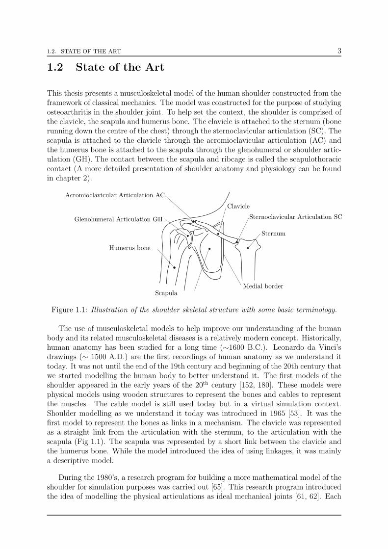
This thesis presents a musculoskeletal model of the human shoulder constructed from theframework of classical mechanics. The model was constructed for the purpose of studyingosteoarthritis in the shoulder joint. To help set the context, the shoulder is comprised ofthe clavicle, the scapula and humerus bone. The clavicle is attached to the sternum (bonerunning down the centre of the chest) through the sternoclavicular articulation (SC). Thescapula is attached to the clavicle through the acromioclavicular articulation (AC) andthe humerus bone is attached to the scapula through the glenohumeral or shoulder artic-ulation (GH). The contact between the scapula and ribcage is called the scapulothoraciccontact (A more detailed presentation of shoulder anatomy and physiology can be foundin chapter 2).
Sternum
Clavicle
Scapula
Humerus bone
Medial border
Sternoclavicular Articulation SC
Acromioclavicular Articulation AC
Glenohumeral Articulation GH
Figure 1.1: Illustration of the shoulder skeletal structure with some basic terminology.
The use of musculoskeletal models to help improve our understanding of the humanbody and its related musculoskeletal diseases is a relatively modern concept. Historically,human anatomy has been studied for a long time (∼1600 B.C.). Leonardo da Vinci’sdrawings (∼ 1500 A.D.) are the first recordings of human anatomy as we understand ittoday. It was not until the end of the 19th century and beginning of the 20th century thatwe started modelling the human body to better understand it. The first models of theshoulder appeared in the early years of the 20th century [152, 180]. These models werephysical models using wooden structures to represent the bones and cables to representthe muscles. The cable model is still used today but in a virtual simulation context.Shoulder modelling as we understand it today was introduced in 1965 [53]. It was thefirst model to represent the bones as links in a mechanism. The clavicle was representedas a straight link from the articulation with the sternum, to the articulation with thescapula (Fig 1.1). The scapula was represented by a short link between the clavicle andthe humerus bone. While the model introduced the idea of using linkages, it was mainlya descriptive model.
During the 1980’s, a research program for building a more mathematical model of theshoulder for simulation purposes was carried out [65]. This research program introducedthe idea of modelling the physical articulations as ideal mechanical joints [61, 62]. Each

4 1.2. STATE OF THE ART
(a) (b)
Humerus Link
Scapula Link
Clavicle Link
SC Sinus Cone
AC Sinus Cone
GH Sinus Cone
Figure 1.2: (a) Illustration of the linkage model introduced by Dempster in 1965 [53].(b) Illustration of the joint sinus cone model introduced by Engin [65], Engin and Chen[61, 62] and Engin and Tumer [63, 64].
joint was attributed a sinus cone, limiting its motion [63, 64]. The apex of the cone wasset at the centre of the joint and the distal link was constrained to remain in the cone(Fig. 1.1). The model produced by this research program was mainly kinematic. Inthe late 80’s, a specific set of coordinates for describing the configuration of the shoulderbones with respect to the sternum was published [103, 104]. The coordinates were used toconstruct a regression model for the kinematics of the clavicle and scapula. This modeldefined the kinematic coordinates of the clavicle and the scapula as functions of thecoordinates of the humerus bone. This model is referred to as the swedish model and wasinitially kinematic. In 1992 and again in 1999, the swedish model was updated to includedynamics and a more accurate representation of the muscles [114, 138]. In 1994, thefirst high fidelity musculoskeletal model of the shoulder to include dynamics in the senseof classical mechanics, was constructed [194]. The model included a one-dimensionalfinite element model of the bones and muscles (Fig. 1.3). It included a model of thescapulothoracic contact, where two points on the scapula’s medial border were constrainedto remain at a constant distance form the surface of an ellipsoid representing the surfaceof the ribcage. The additional distance represented the layer of tissue in between. Themodel was also the first to investigate the most appropriate method of using the cablemuscle model to represent muscles with large attachment sites [197].
The dynamic shoulder model with one-dimensional finite elements is now referred toas the Delft Elbow and Shoulder Model (DSEM). It can be seen as the first exampleof a modern musculoskeletal shoulder model. Indeed, many of its attributes are foundin a number of more recent models. In 1998, a highly detailed musculoskeletal modelfor simulation of a virtual human being was published [142]. This model included allthe bones and muscles as well as the skin. In 2001, a kinematic musculoskeletal modelconstructed from the Visible Human Project (VHP) dataset was developed [74, 76]. Themodel was designed for estimating the properties of a muscle model [77]. It also includeda scapulothoracic contact model identical to the original model from [194]. Also in 2001,a dynamic musculoskeletal shoulder model was published [129]. This model has beenprogressively developed and is now included in the AnyBody R© musculoskeletal modellingsoftware [49]. The model was designed for multiple purposes. In 2005, a dynamic modelof the shoulder was designed for studying the effects of musculoskeletal surgery [101].

1.2. STATE OF THE ART 5
This model is now one of many models available in the Simtk OpenSim musculoskeletalmodelling software [52]. In 2006, a shoulder model was developed for estimating the forcein the glenohumeral joint [37]. This model is sometimes referred to as the Newcastleshoulder model. In 2007, a musculoskeletal shoulder model was developed for analysingergonomy [54]. In 2011, a model of the shoulder was developed for studying the stability ofthe glenohumeral joint [69]. Stability is understood here as keeping the articulation fromdislocating. In 2012, the shoulder model constructed from the Visible Human Project wasgiven a dynamic model [170]. More comprehensive reviews of musculoskeletal shouldermodels can be found in the literature [168, 219].
(a) (b) (c)
Figure 1.3: (a) Illustration of a diagram from the van der Helm musculoskeletal shouldermodel [194]. (b) Illustration of the shoulder model from the AnyBody modelling software[129]. (c) Illustration of the shoulder model from the OpenSim modelling software [101].
A number of numerical methods have been developed in parallel, specifically for mus-culoskeletal models. These methods are designed either to deal with the different chal-lenges arising from constructing a musculoskeletal model, or to simply use the modelefficiently. This dissertation focuses on two families of numerical methods in particular;First, methods for motion planning of the model’s kinematics, and second, methods forcomputing the necessary forces in the muscles to generate a specific motion.The human shoulder is kinematically redundant. There are more internal degrees of free-dom in the shoulder than degrees of freedom of the elbow’s position. Therefore, planningthe kinematics of shoulder models is not straightforward; A number of methods have beendeveloped to deal with the kinematic redundancy such as regression models. As statedpreviously, the swedish model was the first to introduce a coordinate system for describingthe configuration of the bones [103, 104]. A set of three Tait-Bryan angles was defined foreach bone and the coordinates were used to develop a regression model of shoulder kine-matics. The kinematics of the clavicle and scapula where expressed as nonlinear functionsof the kinematics of the humerus. Thus, reducing the number of coordinates to three.This regression model was adapted in 2009 to a Denavit-Hartenberg description of thekinematics [218]. There are other regression models using linear functions [50, 84, 215].

6 1.3. CONTRIBUTIONS
Inverse kinematics was also used in planning the kinematics of a shoulder model [142]. Athird method consists of minimising the difference between the model’s kinematics andmeasured kinematics [8, 156]. The development of kinematic motion planning strategiesfor the shoulder is still a very relevant research topic [211]. Indeed, recent developmentsin motion capture techniques have lead to more accurate descriptions of shoulder kine-matics [58, 199]. Furthermore, a new direction in this research is to construct kinematicdescriptions that are specific to an individual [20].The human shoulder, like many other musculoskeletal systems, is overactuated. There isan infinite number of muscle activation patterns generating the same motion. A numberof methods have been developed to estimate the forces in the muscles of a musculoskeletalsystem that generate a desired movement. The problem is also referred to as the forcesharing problem. A comprehensive review can be found in the literature [66]. Solutionsto this problem are called coordination strategies. A strategy commonly used for theshoulder is inverse dynamics coupled with static optimisation [70, 90, 195]. A kinematicmotion of the model is planned over a time horizon. The motion is then given to aninverse dynamics model yielding the required torques or actuation at each joint. Thetemporal evolution of the joint torques is discretised and a static optimisation problemis defined at each instant, to find the muscle forces that generate the torques, while min-imising a cost function. The problem is subject to a number of constraints representingthe restrictions imposed by the physical system. The optimisation problem is generallyformulated as a nonlinear program and solved using appropriate NLP algorithms. Theoptimisation problem has also been formulated as a quadratic program using the rela-tion between joint torques and muscle forces [3, 190]. This method is called null-spaceoptimisation. The most used cost function is the one minimising the mean square musclestress [194]. This cost function is called the second-order polynomial cost function andis mathematically a quadratic sum of the forces, divided by their cross-sectional area.Another cost function has been introduced called the min/max criterion [6]. This costfunction is shown to produce similar results to the polynomial cost function with higherorders [172]. More recently, energy-based cost functions involving oxygen consumptionhave been formulated [167].
The above presentation is not a comprehensive review of the literature. However, thereferences stated above are viewed as the most relevant to the current work.
1.3 Contributions
The present dissertation is part of a research program funded by the Swiss NationalScience Foundation (SNF)1 to study osteoarthritis. The question driving the researchprogram is the possibility of a neuromuscular dysfunction as the underlying cause of os-teoarthritis. Osteoarthritis in the shoulder occurs mainly in the glenohumeral joint andit causes excessive loading of the joint. The humeral head is pressed into the glenoid.Therefore, the primary motivation behind the present dissertation, is the construction ofa musculoskeletal shoulder model for estimating the intensity of the joint reaction force
1Research grant reference number: K-32K1-122512

1.3. CONTRIBUTIONS 7
in the glenohumeral joint. The shoulder models presented in the previous section can alsobe used for such a study. However, given that the ultimate goal of the research programis to investigate neuromuscular interactions the model is being designed from scratch.Neuromuscular interactions are a control problem and therefore it is necessary to havefull knowledge and access to the model’s content. The model is capable of estimatingthe forces in the muscles and the contact force in the glenohumeral articulation. Thedissertation focuses on the model’s construction. The model is constructed from the lawsof classical mechanics, considering the bones to be rigid bodies, the articulations to beidealised mechanical joints and the muscles to be ideal cables wrapping over the bones.The present model is based on the kinematic musculoskeletal shoulder model constructedfrom the Visible Human Project [74, 76]. The present model adds a dynamic layer interms of equations of motion and uses a modified scapulothoracic contact model.Using the modified contact model, a novel parameterisation of the shoulder’s kinemat-ics is proposed. The parameterisation uses a set of independent minimal coordinatesthat make kinematic computations related to the model, straightforward. The modelformulates the muscle-force estimation problem as a quadratic program and solves it us-ing null-space optimisation [3, 190]. The null-space optimisation, previously published[3, 190], was used in this dissertation to detect weaknesses in the model of the shoulder’smuscle structure. The model was implemented and used to estimate the reaction forcesin the glenohumeral joint during quasi-static and dynamic raising of the outstretched arm(abduction).The present work addresses the topic of neuromuscular control through a brief analysisof a human motor control mechanism called joint stiffness control through antagonisticmuscle co-contraction. This particular mechanism is analysed because it is related tomuscle-force coordination and hence to the joint forces themselves. It is also a mecha-nism controlling a mechanical property of the joints, stiffness. The mechanism is analysedusing a simple model of a cable-driven pendulum. The pendulum model is relevant tothe analysis, given that it shares the same mathematical structure as models of muscu-loskeletal systems. The joint stiffness control mechanism is implemented on a physicalsystem and the results are used to initiate the discussion of neuromuscular control as apossible cause to osteoarthritis.
A second contribution of this dissertation is to propose a formal and precise mathe-matical representation of musculoskeletal shoulder modelling. In general, musculoskeletalmodels are designed for clinical purposes such as analysing osteoarthritis. The models areconstructed and used by both engineers and medical staff, which constitutes a challengewhen presenting one’s work. The message must be understandable for everyone work-ing in the same interdisciplinary field. Therefore, many presentations of musculoskeletalmodels do not include the technical or mathematical details of the model. A point thatmakes it difficult for others to reconstruct the models.Biomechanics and in particular biomechanics of the human shoulder involves researchthat can be classified into four categories. Experimental, theoretical, applied and fun-damental research [47, 48]. Musculoskeletal modelling is situated between theoreticaland fundamental research and is essentially applied physics. Physics describes our uni-verse through a set of principles that are formally expressed as mathematical equations.These principles govern both the macroscopic and microscopic elements of the universe.

8 1.4. ORGANISATION OF THE THESIS
Given that musculoskeletal models are constructed from these principles, the equationsthey involve constitute the model’s blueprint. Presenting the mathematical equationsof a model allows others to reproduce the work and test it more thoroughly. Lastly,presenting the mathematics of a model favours dissemination of technical ”know-how”.Others can profit from a technical description of a model and thereby further improveresearch. Mathematics constitute an important foundation of musculoskeletal modellingand therefore a good portion of this dissertation tries to formalise the principles used toconstruct and work with the model. The work is presented such that technical detailsare given where they are required for others to reconstruct the work. The presentationis not however, entirely technical. A considerable effort has been made such that thepresentations and discussions remain accessible to as wide an audience as possible.
1.4 Organisation of the Thesis
The dissertation, present chapter included, is composed of eleven chapters, organised asfollows:
Chapter 2: Anatomy, physiology and movement of the human shoulder.
The core of the thesis is modelling the human shoulder. Therefore, this chapter presentsan overview of the human shoulder and introduces the system specific vocabulary.
Chapter 3: Multibody systems theory. This chapter gives an extended presenta-tion of single-body and multibody mechanics and defines the notations used throughoutthe thesis. The purpose of this chapter is to construct the technical framework of theentire dissertation.
Chapter 4: A musculoskeletal model of the human shoulder. This chapterpresents the musculoskeletal shoulder model that is being developed for estimating forcesin the glenohumeral joint. The chapter focuses on the model’s construction and math-ematical structure. The chapter also presents the geometric muscle model linking theforces in the muscles to the dynamics of the skeletal system. The chapter concludes byintroducing the idea that models of musculoskeletal systems and models of cable-drivenrobots have similar mathematical structures.
Chapter 5: Coordinated redundancy. This chapter defines the concept of co-ordinated redundancy and sets a specific framework for chapters 6 and 7. The chapterintroduces the idea of using tasks for coordination and introduces the general coordinationstrategy used for the shoulder model.
Chapter 6: Shoulder kinematic redundancy coordination. This chapterpresents a new method of solving the shoulder model’s kinematic redundancy withoutrequiring measured data. The method uses a minimal set of coordinates obtained througha parameterisation of the shoulder girdle as a parallel platform. The coordinates are inde-pendent from each other and significantly simplify the computational aspects of planningmovements for the shoulder model. The coordinates are constructed from a detailed

1.4. ORGANISATION OF THE THESIS 9
analysis of the kinematic shoulder model’s mathematical structure.
Chapter 7: Shoulder overactuation coordination. This chapter presents acoordination strategy for solving the shoulder’s overactuation problem relying on musclemoment-arms. A classical definition of muscle moment-arms is given, followed by twomethods of computing moment-arms. The first is a geometric method and the second isthe well known tendon excursion method. The two methods are shown to not be strictlyequivalent. This chapter defines the necessary conditions for the existence of a solutionto the coordination problem and introduces the concept of wrench-feasibility.
Chapter 8: Estimating joint forces in the human shoulder. This chapterpresents the implementation of the musculoskeletal shoulder model from chapter 4, us-ing the methods described in chapters 6 and 7. The chapter briefly reviews the modeland presents the results that were obtained, including model-estimated scapular kine-matics, muscle moment-arms, muscle forces and most importantly the reaction force inthe glenohumeral joint. The chapter discusses the model’s current capabilities and useswrench-feasibility to explain the results.
Chapter 9: Introduction to control theory. This chapter presents a briefoverview of control theory, giving the essential concepts and definitions used in chap-ter 10.
Chapter 10: Joint stiffness control for musculoskeletal stability. This chap-ter investigates a mechanical stabilisation mechanism used in human motor control. Thechapter demonstrates that the mechanism does achieve stability in the sense of moderncontrol theory. A cable-driven pendulum is used as a tool to present and discuss theinvestigation. The chapter also presents a joint stiffness control strategy that was im-plemented on a physical cable-driven pendulum. The implementation results are used toinitiate a discussion of the possible cause of osteoarthritis.
Chapter 11: Conclusions This chapter summarises the work, draws some moregeneral conclusions and discusses future work.

10 1.4. ORGANISATION OF THE THESIS

Chapter 2
Anatomy, Physiology and Movement
of the Human Shoulder
This chapter presents a brief, descriptive overview of the shoulder’s anatomy and physiol-ogy. The shoulder’s movement is also covered. All the elements described in the chaptercan be found in closed-form in the literature [32, 53, 83].The human musculoskeletal system allows us to move using our muscles and bones. Itis what gives us form and supports our body. The system is comprised of bones, mus-cles, cartilage, tendons, ligaments, joints and connective tissue. These elements define itsanatomy or structure. The role played by each element define its physiology or function.The purpose of this chapter is to introduce some of the terminology that will be usedthroughout the thesis.
2.1 Shoulder Skeletal Anatomy and Physiology
The human shoulder is comprised of three bones and the upper thorax. The thorax canbe defined as the sternum, ribcage and spine (Fig. 2.1). The first bone is the clavicle, asmall elongated bone connected to the sternum at one end and to the scapula at the other.The clavicle protects the neurovascular bundle (nerves and blood vessels) supplying theupper limb. Its serves as a strut between the sternum and scapula, transmitting loadsfrom the upper limb to the central skeletal axis of the body.The second bone is the scapula, a concave triangular bone connected to the clavicleand the humerus. The scapula’s inner edge is called the medial border. The bony ridgerunning outwards from the upper end of the medial border is called the scapula’s spine. Itfinishes at the acromion, the bony protrusion connecting the scapula to the clavicle. Belowthe acromion is another bony protrusion called the coracoid process. This landmarkis used as a muscle and ligament attachment site. Opposite the medial border is thelateral border running from the angulus inferior to the glenoid cavity. The clavicle andscapula together with the thorax define the shoulder girdle.The third bone is the humerus, a long bone connected to the scapula, the radius and the
11

12 2.1. SHOULDER SKELETAL ANATOMY AND PHYSIOLOGY
ulna. Its upper end is called the humeral head, having a spherical shape. Between thehumeral head and elbow, the humerus has a cylindrical shape. Its lower end is triangular.The external points of this shape are the lateral epicondyle and medial epicondyle.
Anterior View
Clavicle
Scapula
Humerus
Sternum
Ribcage
Posterior View
Clavicle
Scapula
Humerus
Spinal Cord
Ribcage
Humeral Head
Acromion
Coracoid Process
Sternal end of Clavicle
Distal end of Clavicle
Scapular Medial Border
Acromion
Lateral Border
Glenoid
Scapular Spine
Humeral Head
Angulus Inferior
Figure 2.1: Illustration of the shoulder’s skeletal anatomy as described in section 2.1.
The bones are joined together by three synovial articulations providing mobility.In synovial articulations, the bones are not directly connected and do not necessarilytouch each other. There is a synovial cavity surrounding the part of the bones thatare in contact. On the surface of each bone at the point of contact, there is layer ofarticular cartilage that is softer than bone and has less friction. The contact is held bydense tissue surrounding the bones called the articular capsules. The first articulation inthe shoulder is called the sternoclavicular articulation (SC) between the sternum and clav-icle (Fig. 2.2). The second articulation is called the acromioclavicular articulation (AC)between the clavicle and scapula. The third articulation is the glenohumeral articulation(GH) between the scapula and humerus. This articulation is commonly referred to as the”shoulder joint” and is the shoulder’s primary articulation. When the joint is loaded, theround shape of the humeral head is pressed against the concave shape of the glenoid cavityon the scapula (Fig. 2.3). The glenoid has an elliptical shape with the long axis directedvertically. When the joint is relaxed, there is a cavity between the bones. Surrounding theglenoid is the glenoid labrum, a fibro-elastic element protecting the edges of the glenoidcavity. At the other end of the humerus is the elbow and humerolulnar articulation (HU).

2.1. SHOULDER SKELETAL ANATOMY AND PHYSIOLOGY 13
Additional structures of the shoulder associated with articulations include ligamentswhich are viscoelastic elements having a passive role. They are used to stabilise themotion of the bones relative to each other. There are capsular ligaments mentionedpreviously stabilising the synovial articulations. Stability is understood as keeping thebones of an articulation in the correct configuration such that the load passing throughthe articulation is not excessive or misaligned with the contact surfaces. Other ligamentsin the shoulder provide added strength to the shoulder. For instance, the conoid ligamentand coracohumeral ligament stabilise the motion of the scapula relative to the clavicleand humerus. Lastly, the flat concave shape of the scapula allows it to glide over theribcage. This contact is called the scapulothoracic joint or gliding plane (ST) and is notan articulation. Its role is mainly kinematic, guiding the scapula’s movements.
Sternoclavicular articulation
Acromioclavicular articulation
Glenohumeral articulation
Coracoacromial ligament
Coracohumeral ligament
Scapulothoracic contact area
Conoid ligament
Figure 2.2: Illustration of the shoulder’s articulations and ligaments as described in sec-tion 2.1. The ligaments are not anatomically exact and were added to the illustration bythe author.
Glenoid Labrum
Glenoid Cavity
Glenoid Cavity
Tendon of the long head
of the biceps brachii
Scapula’s Spine
Scapula’s Spine
Acromial Process
Coracoid Process
Humeral Head
Figure 2.3: Illustration of the glenoid cavity in the glenohumeral joint as described insection 2.1.

14 2.2. SHOULDER MUSCLE ANATOMY AND PHYSIOLOGY
2.2 Shoulder Muscle Anatomy and Physiology
There are 16 muscles actuating the shoulder. These muscles are called skeletal musclesand are comprised of large numbers of parallel fibres. At either end, there are tendonsconnecting the muscle fibres to the bone. The connection with the skeleton that is closestto the body’s central axis (spine) is called the origin. The other connection is called theinsertion. The names of each muscle and their anatomical locations are illustrated infigure 2.4.
Subclavius
Serratus Anterior (upper)
Serratus Anterior (middle)
Serratus Anterior (Lower)
Trapezius
Rhomboid Minor
Rhomboid Major
Levator Scapulae
Pectoralis MinorPectoralis Major
Latissiumus DorsiDeltoid Anterior
Deltoid Middle
Deltoid Posterior
Supraspinatus
Infraspinatus
Subscapularis
Teres Minor
Teres Major
Coracobrachialis
Figure 2.4: Illustration of the shoulder’s muscle structure. Illustrations taken from [83].
The shoulder girdle is defined as the scapula, the clavicle and the upper left- or upperright-hand side of the thorax. The shoulder girdle is differentiated from the shoulderproper because it is the structure attaching the upper limb to the body. There aremuscles actuating the shoulder girdle and muscles actuating the glenohumeral articulationor shoulder joint. The shoulder girdle muscles include:
• trapezius (TRP), serratus anterior (SRA), rhomboid minor (RMN), rhomboid major(RMJ), levator scapulae (LVS), pectoralis minor (PMN).

2.2. SHOULDER MUSCLE ANATOMY AND PHYSIOLOGY 15
These muscles originate on the thorax and insert on the scapula. The superior part ofthe trapezius muscle inserts on the distal end of the clavicle. The trapezius and serratusanterior are the two major muscles of this group. The glenohumeral articulation musclesinclude:
• deltoid (DLT), infraspinatus (INFR), supraspinatus (SUPR), subscapularis (SBSC),teres minor (TMN), teres major (TMJ), coracobrachialis (CRCB).
The deltoid is the primary muscle of this group. The infraspinatus, supraspinatus, teresminor and subscapularis form a group of muscles collectively known as the rotator cuffmuscles. The goal of these muscles is maintaining the stability of the glenohumeral ar-ticulation. Again, stability is understood as keeping the bones of an articulation in thecorrect configuration.There are two additional muscles actuating the entire shoulder: the latissimus dorsi(LTD) and pectoralis major (PMJ). Both muscles originate on the thorax and inserton the humerus thereby influencing the motion of the entire shoulder. The subclavius(SBCL) muscle is of little importance in actuating the shoulder but rather plays a role ofprotecting certain arteries passing beneath the clavicle. If the clavicle breaks, this muscleprotects the underlying arteries from puncture.
Skeletal muscles have a very specific structure. At either end there are tendons linkingthe muscle to the bone and in-between there is the muscle proper. The tendon attachesthe muscle to the bone by dividing into many small fibres that insert into the bone.Internally, a skeletal muscle is made up of a collection of fibres called muscle bundles.Each bundle is made up of a collection of muscle fascicle. Each fascicle is a collection ofmuscle fibres or muscle cells. This structure is similar to steal cables that are made upof many thin wires of steel grouped together into larger cables forming the entire cable.Internally, each muscle fibre is made up of a number myofibrils, similar to the musclefibre but much smaller. Each myofibril is a sequence of sacromeres linked end-to-endby Z-disks. Sacromeres and Z-disks are connected through a noncontracting filamentcalled connectin. The connectin and Z-disks constitute the muscle’s passive behaviour.A sacromere consists of two types of proteins, actin and myosin that can store and releaseenergy by changing shape and constitute the muscles ability to produce force. There aretwo ways in which sacromeres are stacked: serial or parallel. Serial structures lead tomuscles able to contract quickly while parallel structures lead to muscles producing moreforce because of the increased thickness.
There exist two types of fibres in a muscle; The first are called extrafusal muscle fibresand the second are called intrafusal muscle fibres. Extrafusal fibres represent the majorityand constitute the muscle’s strength. Intrafusal fibres are less numerous and act as lengthsensors for the nervous system. When myosin proteins in a muscle release energy, theresult is either a change in length or the production of force without change in length.It will depend on the interaction of the muscle with the skeletal structure. For example,if the force generated by the muscle is insufficient to overcome inertia, there will be nomovement. It is when muscles do not change length, that they produce the maximumforce, this situation is known as isometric contraction. Given that muscle’s have elastic

16 2.3. SHOULDER MOVEMENT
properties, they apply forces even when not active, this is called the force-length behaviour[95]. There is an optimal length at which a muscle can produce its overall maximum activeforce. The maximum amount of force a muscle can produce diminishes when the muscle’slength is not optimal. The active force-length relationship is a bell curve (Fig. 2.5). Thepassive elements also produce force that steadily increases as the muscle’s length increases.The total force produced by a muscle increases as the muscle’s length increases until theoptimal fibre length. Beyond the optimal fibre length, there is a slight decrease followedby a rapid increase. The muscle’s passive resistance to being stretched dominates forhigh values of muscle length. During normal everyday activities, the muscle works in anarea around the optimal fibre length. The muscle’s total force also depends on the rateof change in muscle length. However, this behaviour is more complex and not coveredhere.
Active force
Passive force
Total force
Optimal muscle length
Muscle
Force
Muscle Length
Nominal functioning area
Figure 2.5: Illustration of the typical force-length behaviour of a skeletal muscle as de-scribed in section 2.2.
2.3 Shoulder Movement
Three orthogonal body planes are used to describe the human body and its motion. Ifthe thorax is attributed a frame such that the x-axis and y-axis define the horizontalplane and the z-axis defines the vertical direction. The body planes are parallel to theplanes defined by the thorax frame and are defined as (Fig. 2.6):
• X-Y plane: transverse plane,
• X-Z plane: coronal plane or frontal plane,
• Y-Z plane: sagittal plane.
The scapular plane represents a fourth plane that is necessary to define the shoulder’smotion. It is a plane perpendicular to the transverse plane but rotated around the z-axes

2.3. SHOULDER MOVEMENT 17
by 30. The scapular plane vertically cuts the glenohumeral joint in half.Thoraco-clavicular motion is defined as the motion of the clavicle with respect to thethorax frame. Scapulo-thoracic motion is defined as the motion of the scapula over thethoracic cage with respect to the thorax frame. Thoraco-humeral motion is defined as themotion of the humerus around the glenohumeral joint with respect to the thorax. Scapulo-humeral motion is defined as the motion of the humerus around the glenohumeral jointwith respect to the scapula.
Coronal/Frontal plane Sagittal plane Transverse plane
30
Scapular plane
x
x yy
z z
Figure 2.6: Illustration of the three body planes and the scapular plane.
Each bone has its own specific set of motions. These elementary motions are definedas follows (Fig. 2.7):
• Clavicle:
– axial rotation: Rotation around the clavicle’s longitudinal axes,
– depression/elevation: rotation in the sagital plane,
– retraction (adduction of clavicle)/protraction (abduction of clavicle): rotationin the transverse plane.
• Scapula:
– axial rotation: rotation around the scapula’s spine,
– depression/elevation: rotation around an axis normal to the scapular spine,
– retraction (adduction of scapula)/protraction (abduction of scapula): rotationaround the thoracic cage.
• Humerus:
– axial rotation: rotation around the humerus’s longitudinal axis,
– flexion/extension: rotation in the sagital plane,
– abduction/adduction: rotation in the coronal plane.

18 2.3. SHOULDER MOVEMENT
The arm’s large range of motion is primarily due to the scapulo-humeral rhythm. Thescapulo-humeral rhythm is defined as the coordinated motion of the scapula and thehumerus [43, 118]. If the scapula was to remain stationary during arm movement, thehumerus/arm could at most abduct to 120. Thus, the scapula’s motion contributes up to60 of the arm’s total abduction angle [174]. Healthy scapulo-humeral rhythm is requiredto achieve full 180 abduction.
Clavicle Motions
Scapular Motions
Humeral Motions
Axial Rotation
Retraction
Protraction
Elevation
Depression
Spinal Tilt
Elevation
Depression
Retraction
Protraction
Axial Rotation
Extension
Flexion
Abduction
Adduction
Figure 2.7: Schematic description of shoulder bone motion definitions. Image createdusing ZygoteBodyTM zygotebody.com.
There have been many studies of the scapulo-humeral rhythm to identify its charac-teristics [73, 105, 149]. The modern description decomposes the scapulo-humeral rhythminto three phases. In phase one, the humerus rotates upward to approximately 30 whilethe scapula remains motionless. This is called the settling phase (Fig. 2.8 I.). In phasetwo, the humerus has rotated up to 90 abduction. As the humerus rotates up to 90,the scapula follows its rotation with a ratio of 1/2. For every two degrees of scapulo-humeral rotation, there is one degree of scapulo-thoracic rotation. The humerus hasrotated by 70 with respect to the scapula. The scapula has contributed 20. This iscalled the 1-2 phase (Fig. 2.8 II.). The 1:2 ratio continues up to 150 abduction. Thereis 110 scapulo-humeral rotation and 40 scapulo-thoracic rotation. The third and lastphase of abduction is characterised by a 1:1 ratio. At 180 abduction, there is a 120
scapulo-humeral rotation and 60 scapulo-thoracic rotation. This is called the 1-1 phase.

2.3. SHOULDER MOVEMENT 19
30
20
70
40
110
Figure 2.8: Illustration of the three phase description of the scapulo-humeral rhythm.
This chapter presented the anatomy, physiology and movement of the human shoulder.The remainder of this thesis deals with the construction of a model of this system andthe associated computational methods. The model is built on the principles of generalmultibody mechanics. Therefore, the next chapter gives a presentation of multibodymechanics in order to set the framework and notations used throughout the remainderof the dissertation.

20 2.3. SHOULDER MOVEMENT

Chapter 3
Multibody Systems Theory
3.1 Introduction
Multibody systems theory is the study of the time-dependent behaviour or dynamicsof interconnected bodies that can be either rigid or flexible. Multibody systems theoryis governed by general mechanics and is therefore described by a formal mathematicalframework. Thus, multibody systems modelling requires a the same rigour and formalismfor the theory to be applied appropriately [18, 86, 157]. The goal of this chapter is to givea detailed overview of multibody systems and to introduce the notations and conventionsthat will be used throughout the thesis.
At the core of multibody systems theory is the construction of the nonlinear equationsof motion which are derived from the expressions of a body’s kinematics and mechanicalenergy. One of the principal methods of deriving a body’s equations of motion is theEuler-Lagrange equation. However, the equations of motion alone are insufficient tocompletely analyse the dynamics of interconnected bodies. The equations of motionprovide no information regarding the internal forces or interactions between the bodies.Thus, the Newtonian approach is also necessary to obtain a complete description of eachbody’s dynamics.This chapter is divided into two parts. Part one presents multibody systems theory fora single body beginning with the kinematics of a single rigid body. The kinematics arepresented in the classical sense of position, velocity and acceleration. The equations ofmotion for a single rigid body are derived using the Newtonian approach. The sameequations are used to express the body’s mechanical energy. Part one also covers theduality between Chasles’ theorem in kinematics and Poinsot’s theorem in dynamics.Part two extends the presentation to the case of multiple bodies. The notions of kinematicpairs and kinematic chains are introduced and the interconnections between bodies aredescribed in terms of constraints. This section also defines a system’s forward kinematicmap and the principle of mobility is introduced. The formalism of analytical mechanicsis presented with a focus on virtual displacements and the principles of virtual power andwork. The principle of virtual work is then used to derive the Euler-Lagrange equation.
21

22 3.2. PRELIMINARIES
Section 3.2 covers the fundamental concepts required to build the theory presentedin the following sections. Sections 3.3 and 3.4 present the kinematics and dynamics ofa single rigid body. Section 3.5 extends the presentation to systems of rigid bodies witha presentation of the formalism of analytical mechanics for building the equations ofmotion.
3.2 Preliminaries
3.2.1 Conventions
Space is the boundless three-dimensional extent, or three-dimensional Euclidean space,denoted R
3. A right-handed coordinate system R0 is used to describe space, defined bythree, mutually perpendicular axes, referred to as x, y and z. The intersection point ofthe three axes is the origin O0 of the reference system. To each axis is associated a unitvector i0, j0 and k0. A right-handed reference system is defined such that if one were tograb the z-axis with the right hand, such that the thumb points in the direction of thez-axis unit vector, the fingers would curl around the axis from the x-axis to the y-axis.
xx yy
zzR
px,0 py,0
pz,0
i0 j0
k0
O0
P0~p0
Figure 3.1: Illustration of the right-handed coordinate system and the right hand thumbprinciple as described in section 3.2.1.
The position of a point P0 in space is defined by a vector emanating from the originof the coordinate system to the point (Fig. 3.1). The components for this vector are px,0,py,0 and pz,0. A component of a position vector is positive if the projection of the vectoronto the corresponding coordinate axis points in the same direction as the unit vectorotherwise it is negative.
P0 : ~p0 =(px,0 py,0 pz,0
)T= px,0i+ py,0j + pz,0k0,
px,0 = (~p0 · i0)i0, py,0 = (~p0 · j0)j0, pz,0 = (~p0 · k0)k0.
The point O0 is the only point in the reference system R0 with all three coordinatesequal to zero. The coordinate system’s unit vectors satisfy the orthonormality properties

3.2. PRELIMINARIES 23
in terms of the dot and cross products, defined in the usual manner.
i0 · i0 = j0 · j0 = k0 · k0 = 1, i0 × i0 = j0 × j0 = k0 × k0 = 0,
j0 · k0 = i0 · k0 = i0 · j0 = 0, i0 × j0 = k0, k0 × i0 = j0, j0 × k0 = i0.
The reference frame which is fixed in space is referred to as the inertial reference frameand will be denoted R0. The subindex will always indicate this frame. In the case ofmultiple reference systems, other reference systems will be denoted Ri. The subindexi = 1, 2, 3, ... will always denote a particular frame. Vectors defined in a particular framewill have the associated subindex.
3.2.2 Geometric Configuration
The geometric configuration of a point P0 in space with respect to the inertial frame R0
is simply the coordinates of the point. The geometric configuration C0,i of a body Bi inspace is defined as the position of all its particles. A rigid body is an idealised solid, orcollection of particles, that cannot be deformed. The distance between any two points onthe body remains constant at all times. A free body is an unconstrained body that canmove freely within R
3.
x y
z
R0
~r0,i
~s0,i
~t0,ii0
j0
k0
O0
R0,i
S0,i
T0,i
Bi
Figure 3.2: Illustration of a free rigid-body’s geometric configuration with respect to theinertial reference frame R0 as described in section 3.2.2.
Under the rigid body hypothesis, it is sufficient to know the position of three non-colinear particles to know the geometric configuration of the body. The geometric config-uration C0,i of a free body Bi is defined with respect to the inertial frame by three pointssubject to the rigid-body constraints (3.2).
C0,i :
R0,i : ~r0,i =(rx,0 ry,0 rz,0
)T,
S0,i : ~s0,i =(sx,0 sy,0 sz,0
)T,
T0,i : ~t0,i =(tx,0 ty,0 tz,0
)T,
(3.1)
‖R0S0‖2 = cte, ‖R0T0‖2 = cte, ‖S0T0‖2 = cte. (3.2)
There are nine coordinates subject to three equality constraints meaning that a freerigid-body’s geometric configuration is described by six independent coordinates.
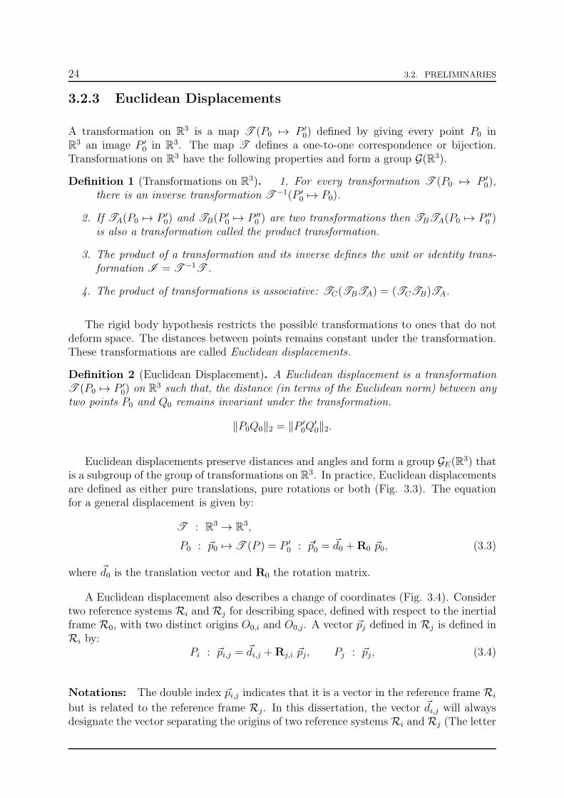
24 3.2. PRELIMINARIES
3.2.3 Euclidean Displacements
A transformation on R3 is a map T (P0 7→ P ′
0) defined by giving every point P0 inR
3 an image P ′0 in R
3. The map T defines a one-to-one correspondence or bijection.Transformations on R
3 have the following properties and form a group G(R3).
Definition 1 (Transformations on R3). 1. For every transformation T (P0 7→ P ′
0),there is an inverse transformation T −1(P ′
0 7→ P0).
2. If TA(P0 7→ P ′0) and TB(P
′0 7→ P ′′
0 ) are two transformations then TBTA(P0 7→ P ′′0 )
is also a transformation called the product transformation.
3. The product of a transformation and its inverse defines the unit or identity trans-formation I = T −1T .
4. The product of transformations is associative: TC(TBTA) = (TCTB)TA.
The rigid body hypothesis restricts the possible transformations to ones that do notdeform space. The distances between points remains constant under the transformation.These transformations are called Euclidean displacements .
Definition 2 (Euclidean Displacement). A Euclidean displacement is a transformationT (P0 7→ P ′
0) on R3 such that, the distance (in terms of the Euclidean norm) between any
two points P0 and Q0 remains invariant under the transformation.
‖P0Q0‖2 = ‖P ′0Q
′0‖2.
Euclidean displacements preserve distances and angles and form a group GE(R3) thatis a subgroup of the group of transformations on R
3. In practice, Euclidean displacementsare defined as either pure translations, pure rotations or both (Fig. 3.3). The equationfor a general displacement is given by:
T : R3 → R
3,
P0 : ~p0 7→ T (P ) = P ′0 : ~p′0 =
~d0 +R0 ~p0, (3.3)
where ~d0 is the translation vector and R0 the rotation matrix.
A Euclidean displacement also describes a change of coordinates (Fig. 3.4). Considertwo reference systems Ri and Rj for describing space, defined with respect to the inertialframe R0, with two distinct origins O0,i and O0,j. A vector ~pj defined in Rj is defined inRi by:
Pi : ~pi,j = ~di,j +Rj,i ~pj, Pj : ~pj, (3.4)
Notations: The double index ~pi,j indicates that it is a vector in the reference frame Ri
but is related to the reference frame Rj . In this dissertation, the vector ~di,j will alwaysdesignate the vector separating the origins of two reference systems Ri andRj (The letter

3.2. PRELIMINARIES 25
xx yy
zz
R0R0
i0i0 j0j0
k0k0
O0O0
~p0~p0
~p′0 = T (~p0)
~d0
R0 ~p0T
Figure 3.3: Illustration of a Euclidean displacement as a translation and a rotation asdescribed in section 3.2.3.
d is specifically reserved for this). The first subindex will always designate the referencesystem in which the vector is explicitly defined. The matrix Rj,i is the rotation matrix,transforming a vector in frame Rj into a vector in frame Ri. For rotation matrices,the order of the subindexes will always indicate the direction of transformations. Rj,i
indicates a transformation from Rj to Ri.
x
x
x
x
y
y
y
y
z
zz
z
R0
Ri
Rj
Rji0 j0
k0
ii
ji
ki
ijij jj
jj
kj
kj
Oi
Oj
Oj
O0
~di,j
~pi,j = T (~pj)
Rj,i ~pj~pj
PiPj
Figure 3.4: Illustration of a Euclidean displacement as a coordinate transformation asdescribed in section 3.2.3.
Euclidean displacements can be expressed as linear applications using homogeneouscoordinates. The entire transformation is grouped into a single matrix Hj,i.
(~pi,j1
)
=
(
Rj,i | ~di,j0 0 0 | 1
)(~pj1
)
= Hj,i
(~pj1
)
, ~pj ≡ ~pj,i. (3.5)
The inverse transformation is defined by
(~pj,i1
)
=
(
Ri,j | −Ri,j~di
0 0 0 | 1
)(~pi1
)
= Hi,j
(~pi1
)
, ~pi ≡ ~pi,j. (3.6)
26 3.2. PRELIMINARIES
The geometric description of a body’s configuration is more appropriate for describingfixed configurations. Euclidean displacements are more appropriate for describing thechange in configuration of a rigid body, i.e. a body’s kinematics. The geometric andEuclidean displacement descriptions are related. Given the geometric description in termsof the points R0, S0 and T0 in a frame Ri, the Euclidean displacement from Rj to Ri isdefined by:
~di,j = ~ri,j, Rj,i =
(
~si,j−~ri,j‖~si,j−~ri,j‖2
(~ti,j−~ri,j)×(~si,j−~ri)
‖(~ti,j−~ri,j)×(~si,j−~ri,j)‖2
((~si,j−~ri,j)×(~ti,j−~ri,j))×(~si,j−~ri,j)
‖((~si,j−~ri,j)×(~ti,j−~ri,j))×(~si,j−~ri,j)‖2
)
.
(3.7)The columns of the matrix Rj,i are the base vectors ij, jj and kj described in the frameRi: ii,j, ji,j and ki,j.
3.2.4 Rotation Matrices
A general 3 × 3 rotation matrix is a way of representing a rotation defining a transfor-mation between two orthonormal representations of space. Rotation matrices satisfy thefollowing properties.
Properties 1. (Rotation matrices)
1. For a rotation matrix R0, there exists another matrix R−10 = R
T0 such that R0R
T0 =
I (Identity matrix).
2. For two rotation matrices R0 and R′0, the product R0R
′0 = R
′′0 is also a rotation
matrix.
3. The composition operation is not commutative R0R′0 6= R
′0R0.
Consider a rotation Ri defined in a frame Ri and a change of coordinates Ri,j. Thesame rotation is defined in the frame Rj by:
Ri,jRiRTi,j = Rj. (3.8)
This is valid for any frame two frames Ri and Rj and leads to the following statement.The rotation matrices Ri and Rj are said to be equivalent and are two representativesof a class of mutually orthogonal matrices. All the classes of such matrices under thecomposition operation form a non-commutative group O(3) of dimension three. Theelements of this group represent both proper and improper rotations. Proper rotationspreserve orientation or right-handedness of the coordinate frame, improper rotations donot. In rigid-body mechanics, only proper rotations are used. The rotation matricesrepresenting proper rotations satisfy the additional property.
Proper Rotation: det(Ri) = 1, Improper Rotation: det(Ri) = −1. (3.9)
All rotation matrices representing proper rotations form the subgroup SO(3) of O(3)called the special orthogonal group. This group will be discussed in section 3.2.5.

3.2. PRELIMINARIES 27
The components of a rotation matrix Rj,i are the direction cosines of the coordinateframe unit vectors. Direction cosines are the projections of the unit vectors of frame Rj
onto the unit vectors of Ri. i.e. the cosines of the angles between the reference framevectors.
ii,j · ji = cos (∠(ii,j, ji)) . (3.10)
Notation: A reference frame unit vector with double subindex ii,j means the vectoris a unit vector of the frame j indicated by the second index but defined in the frame iindicated by the first index.
The columns of Rj,i are the unit vectors of Rj , defined in Ri.
Rj,i =(ii,j ji,j ki,j
),
ii,j =(ii,j · ii ii,j · ji ii,j · ki
)T,
ji,j =(ji,j · ii ji,j · ji ji,j · ki
)T,
ki,j =(ki,j · ii ki,j · ji ki,j · ki
)T.
(3.11)
3.2.5 Angular Description of Rotations
As mentioned previously, rotations in multibody systems are elements of SO(3). SO(3)is a non-commutative group of dimension three, subgroup of O(3). The group is a Liegroup with a natural smooth manifold1 structure, diffeomorphic2 to the real projectivespace P
3 [99, 100].3 This can be understood as there exist smooth, invertible maps orcharts between subsets of R3 and SO(3). Thus, three independent variables are needed todescribe a rotation. There are many charts on SO(3) defining coordinate systems. Themost well known examples of charts on SO(3) are Euler angles and Tait-Bryan angles.Both charts are based on the following statement:
A general rotation in R3 is built and determined by three successive planar rotations
in three mutually orthogonal planes.
Leonard Euler, [67]
If the three rotations occur in the same frame, the rotation sequence is extrinsic. Ifthe rotations occur in the intermediate frames, the rotation sequence is intrinsic. Eulerangles and Tait-Bryan angles define charts mapping [−π, π]× [−π, π]× [−π, π] ⊂ R
3 toSO(3). The Euler and Bryan angle descriptions of rotations are the most prominent butdefine local charts on SO(3). There is a one-to-one correspondence between a rotationmatrix and its Euler or Bryan angles but this correspondence cannot be defined for everyset of angles. Both charts become singular at certain points, a problem known as gimballock 4. There exist multiple sets of rotation angles yielding the same rotation matrix.
1A smooth manifold is a space of dimension n which locally looks like Rn (cf. chapter 6).
2The term diffeomorphism designates that there is a smooth invertible map between SO(3) and P3.
3The real projective space P3 is comprised of all the lines in R
4 passing through the origin.4Gimbal lock: was coined because the mechanism used to measure the angles is called a gimbal.

28 3.2. PRELIMINARIES
The difference between the Euler and Bryan angle descriptions is the order of therotation. Each planar rotation is defined by an angle: ψ, ϑ and ϕ. For Euler angles, thefirst and third rotation axes are the same. For Bryan angles, all three rotation axes aredifferent. There are two sets of six rotation sequences.
• Euler sequences :(
x− y − x, x− z − x, y − x− y, y − z − y, z − x− z, z − y − z)
,
• Bryan sequences :(
x− y − x, x− z − x, y − x− y, y − z − y, z − x− z, z − y − z)
.
For Euler angles, independently of the sequence, the first angle is the spin angle, thesecond angle is nutation and the third angle is precession. For Bryan angles, the firstangle is roll, the second pitch and the third yaw (Bryan angles are often used to describean aircraft’s configuration). In this presentation, only intrinsic sequences are considered.Intrinsic sequences define a change of coordinates between two reference frames Ri andRj .
(a) (b)
x x
y y y y
zz zz
x′
x′
x′
x′
y′ y′
z′
z′
z′
z′
x′′
x′′ x′′
y′′ y′′ y′′ y′′z′′
z′′
z′′
x′′′
x′′′
y′′′
y′′′
z′′′
z′′′
ψ ψ
ϑ ϑϕ ϕ
R(ψ)R(ψ)
R(ϑ)
R(ϕ) R(ϕ)
RT (θ)Ri,j(ψ, θ, φ)Ri,j(ψ, θ, φ)
RiRi R′
iR′
i
R′
jR′
j Rj
Rj
Figure 3.5: Illustration of (a) the x − y − x Euler angle sequence and (b) the x − y − zBryan angle rotation sequence as described in section 3.2.5.
The intrinsic x− y− x Euler angle sequence from Ri to Rj is defined as follows (Fig.3.5 (a))
Ri,j(ψ, θ, φ) = R(φ) ·RT (θ) ·R(ψ), (3.12)
where
R(ψ) =
(1 0 00 cos(ψ) − sin(ψ)0 sin(ψ) cos(ψ)
)
, R(ϑ) =
(cos(ϑ) 0 − sin(ϑ)
0 1 0sin(ϑ) 0 cos(ϑ)
)
, R(ϕ) =
(1 0 00 cos(ϕ) − sin(ϕ)0 sin(ϕ) cos(ϕ)
)
.
The first rotation R(ψ) can be viewed as a map from Ri to R′i. The second rotation
R(ϑ) can be viewed as a map from R′i to R′
j . The last rotation R(ϕ) maps R′j to Rj .
Euler sequences becomes singular if the nutation angle ϑ = nπ (n ∈ Z), then the first

3.2. PRELIMINARIES 29
and third rotation axes coincide. The intrinsic x − y − z Bryan angle sequence from Ri
to Rj is defined as (Fig. 3.5 (b))
Ri,j(ψ, θ, φ) = R(φ) ·RT (θ) ·R(ψ), (3.13)
where
R(ψ) =
(1 0 00 cos(ψ) − sin(ψ)0 sin(ψ) cos(ψ)
)
, R(ϑ) =
(cos(ϑ) 0 − sin(ϑ)
0 1 0sin(ϑ) 0 cos(ϑ)
)
, R(ϕ) =
(cos(ϕ) − sin(ϕ) 0sin(ϕ) cos(ϕ) 0
0 0 1
)
.
The Tait-Bryan sequence can also be viewed as a sequential change of reference frames.Tait-Bryan sequences become singular when ϑ = nπ
2(n = 2m+1, m ∈ Z). The elementary
rotation matrices are defined such that positive values of the angles yield counterclockwiserotations. Thus, both descriptions are valid for right-handed, orthonormal axes systems,according to the right-hand rule. There is no universal convention regarding the angulardescription of rotation matrices. Therefore, it becomes essential to always give the specificsequence and convention used. This will always be done throughout the presentation.
3.2.6 Euler’s Rotation Theorem
The following theorem regarding rotations is of particular importance. Instead of con-sidering each rotation as a sequence of three rotations around the reference frame axes,Euler considered a single rotation around a particular axis. This theorem is based on theproperty that all direct rotations have an eigenvalue of +1.
Theorem 1 (Euler’s Theorem [67]). For any rotation around a reference frame, thereis a line passing through the reference frame origin such that, all points on this line areinvariant under the rotation.
Stated differently, a sequence of three planar rotations, is equivalent to a single rota-tion about an axis that runs through the centre of the frame by an angle γ. The direction~n of the rotation axis is the eigenvector of the rotation matrix associated to the eigenvalue+1.
~n0 = R0 ~n0, cos(γ) =trR0 − 1
2. (3.14)
A vector ~p0 is related to its image ~p′0 by a rotation around an axis ~n0 of an angle γ,through the following relation (Fig. 3.6)
~p′0 = R0 ~p0 = ~p0 + (1− cos(γ))~n0 × (~n0 × ~p0) + sin(γ)~n0 × ~p0. (3.15)
The rotation matrix can be expressed in terms of the coordinates of ~n and the angle γ.
R0 =
(n2x,0+(1−n2
x,0) cos(γ), nx,0ny,0(1−cos(γ))+nz,0 sin(γ), nx,0nz,0(1−cos(γ))−ny,0 sin(γ)
nx,0ny,0(1−cos(γ))−nz,0 sin(γ), n2y,0+(1−n2
y,0) cos(γ), ny,0nz,0(1−cos(γ))+nx,0 sin(γ)
nx,0nz,0(1−cos(γ))+ny,0 sin(γ), ny,0nz,0(1−cos(γ))−nx,0 sin(γ), n2z,0+(1−n2
z,0) cos(γ)
)
.
(3.16)

30 3.3. RIGID-BODY KINEMATICS
Based on this description of the rotation matrix, the following quantities are called Euler-Rodrigues parameters.
κ0 = cos(γ
2
)
, κ1 = nx,0 sin(γ
2
)
, κ2 = ny,0 sin(γ
2
)
, κ3 = nz,0 sin(γ
2
)
. (3.17)
If grouped into a vector, these four variables constitute a quaternion.
The quaternion description of rotations is more suited to the structure of SO(3).SO(3) is a three-dimensional manifold embedded in a four dimensional space. A quater-nion is a four dimensional vector subject to an equality constraint. The quaternion chartremains three-dimensional because of the unit length constraint. While quaternions avoidthe problem of singularities, they are more difficult to use for analysing kinematics. There-fore, in many situations the angle description is used because only a portion of SO(3) isconsidered.
x y
zR0
i0j0
k0
~n0
γ
~p0
~p′0
Figure 3.6: Illustration of Euler’s Theorem as described in section 3.2.6.
3.3 Rigid-Body Kinematics
Kinematics studies the motion of points, bodies and systems of bodies in space withoutconsidering the possible causes. The study of the properties of motion not dependingon time is called geometric kinematics. The study of time-dependent properties is calledinstantaneous kinematics. This section presents the instantaneous kinematics for a singlerigid body. The classical description of a single-body’s kinematics is also given in termsof position, velocity and acceleration. The Poisson formula for rotating vectors is givenas well as the fundamental transport theorem. This section ends with Chasle’s theoremfrom screw theory and the instantaneous screw axis.
3.3.1 Instantaneous Angular velocity
Consider a point X0,i fixed in Ri but rotating around the inertial frame R0. The locationof the point at a given instant is defined by:
X0,i(t) : ~x0,i(t) = Ri,0(t)~xi. (3.18)

3.3. RIGID-BODY KINEMATICS 31
where ~xi is the location of the point in the frame Ri. This point has an instantaneouslinear velocity.
X0,i(t) : ~x0,i(t) = Ri,0(t)~xi = Ri,0R−1i,0~x0,i(t) = Ω0,i(t)~xi(t). (3.19)
The matrix Ω0,i is called the instantaneous rotational velocity matrix. It is a skew-symmetric matrix. Rotational motion is instantaneously described by a single set ofskew-symmetric matrices. Take the infinite taylor expansion of the rotation matrix.
Ri,0(t) = I+R1t+1
2!R2t
2 +1
3!R3t
3 + . . . . (3.20)
Each of the matrices Rk can be written as the sum of a symmetric and skew symmetricmatrix.
Ri,0(t) = I+ (C1 +B1)t+1
2!(C2 +B2)t
2 +1
3!(C3 +B3)t
3 + . . . . (3.21)
The symmetric matrices Ck can be expressed in terms of the matrices Bk according tothe recursion formula, given that C1 = 0.
Ck =−1
2
k−1∑
j=1
(kj
)
(Ck−j +Bk−j) (Cj −Bj) . (3.22)
Following these relations, the instantaneous rotational velocity matrix is defined by:
Ω0,i(t) = Ω0 +Ω1t+1
2Ω2t
2 + . . . , Ωk =k+1∑
j=1
(k
j − 1
)
(Cj +Bj) (Ck−j+1 −Bk−j+1). (3.23)
Using (3.22) leads to the following results:
Ω0 = B1, Ω1 = B2, Ω2 = −B31 +
1
2(B1B2 −B2B1) +B3. (3.24)
Thus, only the matrices Bk describe rotational motion in and around a given instant(t = 0). Indeed, the matrices Bk result from a temporal linearisation. The linearisedrotation matrix describes the rotation from a moment shortly before the instant (−δt) toa moment shortly after (δt). The matrix Ω0,i has three independent elements and alwayshas the form:
Ω0,i =
0 −ωz ωyωz 0 −ωx−ωy ωx 0
. (3.25)
Because the matrix has this form, the velocity of the point X0,i is also defined by
X0,i(t) : ~x0,i(t) = ~ω0,i(t)× ~x0,i(t), ~ω0,i =(ωx ωy ωz
)T. (3.26)
This is the fundamental formula defining the velocity for rotating vectors. This formulais sometimes referred to as the Poisson formula.

32 3.3. RIGID-BODY KINEMATICS
3.3.2 Instantaneous Kinematics
Given a rigid body Bi, with a reference frame Ri, moving in space with respect to theinertial frame R0. The position of any point X0,i on the body in the inertial frame, at agiven instant t is defined by a Euclidean displacement.
X0,i(t) : ~x0,i(t) = ~d0,i(t) +Ri,0(t) ~xi = ~d0,i(t) + ~x∗0,i(t). (3.27)
This definition of Euclidean displacement is fundamental and will be continuously used inthis presentation. A vector with a star indicates that it is a rotated vector. The positionof the point X0 is defined by a polynomial of time.
X0,i : ~x0,i = ~x1 + ~d0 +(
B1~x1 + ~d1
)
t+
1
2!
(
(C2 +B2)~x1 + ~d2
)
t2 +1
3!
(
(C3 +B3)~x1 + ~d3
)
t3 + . . . . (3.28)
Each coefficient of the polynomial is a itself a Euclidean displacement.
~xk = ~dk + (Ck +Bk)~x1. (3.29)
The velocity and acceleration are defined by:
X0,i : ~x0,i = B1~x1 + ~d1 +(
(C2 +B2)~x1 + ~d2
)
t +1
2
(
(C3 +B3)~x1 + ~d3
)
t2 + . . . ,
(3.30)
X0,i : ~x0,i =(
(C2 +B2)~x1 + ~d2
)
+(
(C3 +B3)~x1 + ~d3
)
t+ . . . . (3.31)
All the matrices Bk can be reduced to a set of vectors ~bk, using the definition of the in-stantaneous angular velocity matrix. The position, velocity and acceleration are thereforealso defined by vectors.
X0,i : ~x0,i =~x1 + ~d0 +(
~b1 × ~x1 + ~d1
)
t+
1
2
(
−(~b1 ·~b1)~x1 + (~b1 · ~x1)~b1 +~b2 × ~x1 + ~d2
)
t2 + . . . (3.32)
X0,i : ~x0,i =~b1 × ~x1 + ~d1 +(
−(~b1 ·~b1)~x1 + (~b1 · ~x1)~b1 +~b2 × ~x1 + ~d2
)
t+ . . . (3.33)
X0,i : ~x0,i =(
−(~b1 ·~b1)~x1 + (~b1 · ~x1)~b1 +~b2 × ~x1 + ~d2
)
+(3
2(~b1 · ~x1)~b2 +
3
2(~b2 · ~x1)~b1 − 3(~b1 ·~b2)~x1 +~b3 × ~x1~d3
)
t . . . (3.34)
Instantaneous kinematics studies the low order terms of these expansions. The vectors ~b1and ~b2 are the instantaneous angular velocity and angular acceleration vectors at t = 0.These terms, along with ~b3 and ~b4 are used to construct the instantaneous kinematicinvariants [23].

3.3. RIGID-BODY KINEMATICS 33
3.3.3 Movement: Velocity and Acceleration
As stated in section 3.2.2, six parameters are necessary to parameterise the geometricconfiguration of a free body Bi in space. A euclidean displacement parameterises theposition of a body as the linear position of the body frame’s centre O0,i (in the inertialframe) and the orientation of a point X0,i (in the inertial frame) with respect to the centreof the body frame.
X0,i : ~x0,i = ~d0,i +Ri,0~xi = ~d0,i︸︷︷︸
linear position
+ ~x∗0,i︸︷︷︸
orientation
.
The asterisk symbol on a vector always is used to shorten the notation. It will alwaysmean the following ~x∗j,i = Ri,j~xi. The six coordinates parameterising the body’s geometricconfiguration are the three translational coordinates of the reference frame origin and thethree rotation angles. The kinematics of a rigid body are parameterised in terms of thevector of kinematic coordinates and its derivatives.
~qi =
(xi yi zi︸ ︷︷ ︸
~ΓTi
ψi ϑi ϕi︸ ︷︷ ︸
~ΥTi
)T
= (~ΓTi ,~ΥTi )
T ∈ SE(3). (3.35)
The vector ~Γi is the translational coordinate vector and the vector ~Υi is the rota-tional coordinate vector. The subindex i indicates that the coordinates parameterisethe kinematics of body Bi. The vector of kinematic coordinates belongs to the setSE(3) = R
3 × SE(3) called the special Euclidean group. The group acts on elements ofR
3 through homogeneous transformations defined in section 3.2.3.
X0,i :
(~x0,i1
)
= Hi,0
(~xi1
)
=
(
Ri,0 | ~d0,i0 0 0 | 1
)(~xi1
)
. (3.36)
The matrix Hi,0 is an element of SE(3). Given that SE(3) is composed of R3 and SO(3),it is also a Lie group with a smooth manifold structure. The velocity of a point on thebody in the inertial frame is defined by:
X0,i(~qi) : ~x0,i = ~d0,i +Ri,0~xi, (3.37)
X0,i(~qi, ~qi) : ~x0,i = ~d0,i + ~ω0,i × ~x∗0,i. (3.38)
This is called the fundamental transport theorem. Using the Poisson formula again, theacceleration of the point X0,i is defined by the relation
X0,i(~qi, ~qi, ~qi) : ~x0,i = ~d0,i + ~ω0,i × ~x∗0,i + ~ω0,i ×(~ω0,i × ~x∗0,i
), (3.39)

34 3.3. RIGID-BODY KINEMATICS
Theorem 2 (Rigid-Body Kinematics (Classical Description)). The spatial kinematicsof a single free rigid-body Bi, fixed in the body frame, are defined with respect to theinertial frame R0, by the following set of equations:
X0,i : ~x0,i = ~d0,i +Ri,0~xi, (3.40)
X0,i : ~x0,i = ~d0,i + ~ω0,i ×Ri,0~xi, (3.41)
X0,i : ~x0,i = ~d0,i + ~ω0,i ×Ri,0~xi + ~ω0,i × (~ω0,i ×Ri,0~xi) . (3.42)
where ~d0,i is the pure translational motion. Ri,0 is the rotation matrix defining therotational motion of the body and ~ω0,i is the instantaneous rotational velocity vectorwith respect to the inertial frame.
The instantaneous angular velocity vector is defined according to the rotation se-quence. Consider the x− y − z Tait-Bryan sequence defined previously in section 3.2.5.The velocity vector is parallel to the rotation axis and its direction gives the directionof rotation, according to the right-hand rule (clockwise (-) / counterclockwise (+)). Thebody is first rotated around the x-axis. Its first component is therefore defined by:
R(ϕi)RT (ϑi)R(ψi)
ψi00
.
The second rotation occurs around the y-axis of the first intermediate rotated frame R′i
(cf. Fig. 3.5).
R(ϕi)RT (ϑi)R(ψi)
ψi00
+R(ϕi)RT (ϑi)
0
ϑi0
.
The third rotation occurs around the z-axis of the second intermediate rotated frame R′0
(cf. Fig. 3.5).
~ω0,i(ψi, ϑi, ϕi) = R(ϕi)RT (ϑi)R(ψi)
ψi00
+R(ϕi)RT (ϑi)
0
ϑi0
+R(ϕi)
00ϕi
. (3.43)
The instantaneous rotational velocity vector can also be expressed in the body frame. Itdefines the rotation of the inertial frame with respect to the body frame.
~ωi = R0,i~ω0,i. (3.44)
The rotational velocity vector is a linear function of the angular velocities ~Υi. The vector
can be express in terms of its jacobian with respect to ~Υi.
~ω0,i =∂~ω0,i
∂ψiψi +
∂~ω0,i
∂ϑiϑi +
∂~ω0,i
∂ϕiϕi =
∂~ω0,i
∂~Υi
~iΥ = W0,i(~Υi)~Υi. (3.45)

3.3. RIGID-BODY KINEMATICS 35
The matrix W0,i is a 3×3 invertible matrix depending on the angle sequence and will beextensively used in rigid-body dynamics (Section 3.4). This matrix does become singularfor certain values of Euler and Bryan angle sequences. A similar map is defined for therotational velocities in the body frame.
Theorem 3 (Rigid-Body Kinematics (Parametric Description)). The spatial kine-matics of a single free rigid-body Bi, fixed in the body frame, are parameterised withrespect to the inertial frame R0, in terms of the kinematic coordinates ~qi = (~ΓTi ,
~ΥTi )
T ,by the following set of equations:
~x0,i(~Γi, ~Υi) =~Γi +Ri,0(~Υi)~xi = ~Γi + ~x∗0,i(~Υi), (3.46)
~x0,i(~Γi, ~Υi, ~Γi, ~Υi) =~Γi +W0,i(~Υi)~Υi × ~x∗0,i(~Υi), (3.47)
~x0,i(~Γi, ~Υi, ~Γi, ~Υi, ~Γi, ~Υi) =~Γi +(
W0,i(~Υi)~Υi + W0,i(~Υi)~Υi
)
× ~x∗0,i(~Υi)+
W0,i(~Υi)~Υi ×(
W0,i(~Υi)~Υi × ~x∗0,i(~Υi))
. (3.48)
~Γi = (xi, yi, zi)T is the vector of linear translational kinematic coordinates, ~Υi =
(ψi, ϑi, ϕi)T is the vector angular/rotational kinematic coordinates. W0,i is the jaco-
bian of the instantaneous rotational velocity vector with respect to ~Υi.
3.3.4 Chasles’ Theorem and the Instantaneous Screw Axis
Euler’s theorem states that every rotation takes place about a single axis. A corollary toEuler’s theorem is Chasles’ theorem, obtained by allowing the rotation axis to translatein space.
Theorem 4 (Chasles’ Theorem [39]). General rigid body displacements can be reducedto a translation along a line followed by a rotation about that line.
The motion described in Chasles’ theorem is a screw motion. The translation axis iscalled the screw axis. Mathematically, a screw S is a pair of three dimensional vectors[12]. Geometrically, the pair represents a line in space of direction ~n0 with an associatedpitch ps, ratio between linear and angular quantities. The screw encodes a helical vectorfield (Fig. 3.7). The screw of a point X0 is defined by:
SX0 =(~n0 ps~n0 + ~n0 × ~r0
), ‖~n‖2 = 1. (3.49)
~r0 is the vector from X0 to the screw axis, normal to the screw axis. In kinematics ascrew encodes a velocity field. The Euclidean displacement associated to a screw motionis called a twist T . A twist is a screw with a scalar called the magnitude equal to ‖~ω0,i‖2.The translation along the axis is equal to the magnitude times the pitch pt.

36 3.3. RIGID-BODY KINEMATICS
Screw Axis
~n0
2πps
~n0 × ~r0
ps~n0~r0
X0
Figure 3.7: Illustration of a screw encoding a helical vector field as described in section3.3.4.
To construct the screw axis for a body Bi, consider a point X0,i on the screw axis.
X0,i : ~x0,i = ~d0,i +Ri,0~xi = ~d0,i + ~x∗0,i, X0 : ~x0,i = ~d0,i + ~ω0,i × ~x∗0,i.
The vector ~x∗0,i is decomposed into a parallel and normal components to ~ω0,i.
~x∗0,i = ~x∗0,i,‖ + ~x∗0,i,⊥, ⇒ ~x0,i = ~d0,i + ~ω0,i × ~x∗0,i,⊥, ~ω0,i × ~x∗0,i,‖ = ~0
Instantaneously, all the points on the screw axis have the same velocity proportional to~ω0,i. The proportionality factor is the pitch pt.
pt~ω0,i = ~d0,i + ~ω0,i × ~x∗0,i,⊥,
By dot- and cross-multiplying this relation by ~ω0,i and using the perpendicularity of ~x∗0,i,⊥with respect to ~ω0,i, yields the following relations [213]:
~x∗0,i,⊥ =~ω0,i × ~d0,i~ω0,i · ~ω0,i
, pt =~ω0,i · ~d0,i~ω0,i · ~ω0,i
. (3.50)
If the body’s reference frame is placed on the instantaneous screw axis, the position ofany point Y0,i (not on the axis) is defined with respect to the inertial frame by:
Y0,i : ~y0,i = ~d0,i + ~x∗0,i,⊥ + ~y∗0,i =~d′0,i + ~y∗0,i, (3.51)
and the velocity of the point Y0,i on the body is defined by:
Y0,i : ~y0,i = ps~ω0,i + ~ω0,i × ~y∗0,i,⊥, (3.52)
where ~y∗0,i,⊥ is the vector from the screw axis to the point Y0,i normal to the screw axis.The point has a translational velocity parallel to the screw axis defined by ~ω0,i and pro-portional to the norm of the rotational velocity.

3.3. RIGID-BODY KINEMATICS 37
For rigid body motion, the twist is in general time variant and therefore one definesthe instantaneous screw axis (ISA). The instantaneous twist is mathematically definedby its screw. This screw completely defines the body’s motion.
TY0,i(t) =(~ω0,i(t) ps(t)~ω0,i(t) + ~ω0,i(t)× ~y∗0,i,⊥(t)
). (3.53)
The norm of the instantaneous rotational velocity vector and the pitch of the screware the first two instantaneous kinematic invariants mentioned in section 3.3.2. Theinstantaneous screw axis defines a ruled surface5 in the inertial frame and the bodyframe.
Screw Axis
Screw Axis
Ri
Ri
X0,i
R0
R0
~y0,i
~x∗0,i,⊥~x∗0,i,‖
Y0,i Y0,i
~d0,i
~x∗0,i~ω0,i
p · ~ω0,i
ω0,i × ~y∗0,i,⊥
~y∗0,i,⊥
~d′0,i
~d′0,i
~y∗0,i
Figure 3.8: Illustration of the construction of the instantaneous screw axis as describedin section 3.3.4.
5A ruled surface S is such that at every point P on the surface, there is a line passing trough thepoint which is also on the surface.

38 3.4. RIGID-BODY DYNAMICS
3.4 Rigid-Body Dynamics
Rigid-body dynamics relates motion to its cause, it expresses the time-dependent be-haviour of rigid bodies under external influences. There are multiple aspects of rigid-bodydynamics. The equations of motion describe how a body moves under the influence offorces. There is the energetic aspect defining how much energy a body has and how muchenergy is being given to it or taken away from it. This section describes both aspects andcovers Newtonian mechanics for a single rigid body. The presentation begins with New-ton’s and Euler’s laws of motion and the definitions of forces and moments of force. Theinertia and moment of inertia of a body are also covered in this section. The equationsof motion are derived and the presentation ends with considerations on the mechanicalenergy of a rigid body.
3.4.1 Newtonian Mechanics
The governing laws of rigid body dynamics are Newton’s three laws which, completelydefine what causes translational motion.
Theorem 5. (Newton’s laws of motion)
1. When viewed in an inertial reference frame, a body Bi either remains at restor continues to move at a constant velocity, unless acted upon by an externalforce.
2. ~f0,i = mi~x0,i: the vector sum of the forces ~f0,i on a body Bi (in the inertialframe) is equal to the mass mi of that body multiplied by the acceleration vector~x0,i of the body, in the inertial frame R0.
3. When one body Bi exerts a force on a second body Bj, the second body Bj
simultaneously exerts a force equal in magnitude and opposite in direction onthe first body Bi.
The first law states that any change in a rigid body’s motion is caused by the action ofan external force. It is the most fundamental law. For there to be motion, there must be aforce. The second law states that the motion of a rigid body, defined by its acceleration,is related to the forces acting on it. Newton’s second law provides a tool for computingthe translational dynamics of a rigid body, described by the equations of motion. Thethird law defines the interactions between rigid bodies. When two bodies are in contact,they exert a force on each other. Thus, forces are the underlying cause of any motionand will be discussed first.

3.4. RIGID-BODY DYNAMICS 39
Newton’s laws constitute only half the equations of motion of a rigid body. The secondlaw governs the translational dynamics only. The rotational dynamics are governed byEuler’s laws of motion. They are as important as Newton’s laws of motion but are lesswell known because they were discovered later.
Theorem 6. (Euler’s laws of motion)
1. The linear momentum of a body ~p0,i, is equal to the product of the mass of thebody mi and the velocity of its centre of mass x0,i in the inertial frame R0:
~p0,i = mi~x0,i.
2. The rate of change of angular momentum ~l0,i with respect to the centre of theinertial frame R0, is equal to the sum of the external moments of force ~t0,i aboutthat point: l0,i = ~t0,i.
The first law is a restatement of Newton’s second law, but is more general. Euler’sformulation of the law is more general in that it incorporates the possibility of a time-dependent mass. This occurs in rockets where the mass drops as the fuel is spent. Euler’ssecond law is the analogue of Newton’s second law for rotational dynamics. It is usedto obtain the rotational part of the equations of motion (if the body can rotate). The
angular momentum ~l0,i contains the angular acceleration vector ~Υi.
3.4.2 Forces, Moments of Force and Poinsot’s Theorem
A force is defined as any external action on a rigid body leading to a change in configura-tion or movement of the body. Physically, only the effect of forces can be measured andnot the forces themselves. There are internal and external forces. Internal forces are forinstance the interaction forces at the atomic level that depend on the material [22, 46].Internal forces are eliminated by the rigid body hypothesis and are thus not consideredin the remainder of this presentation. External forces are either the result of a contactwith another body or the effect of a force field like gravity or electromagnetism. Thefirst are called contact forces, the second are called body forces. There are concentratedforces, applied to a single point or distributed forces, applied along a line, over a surfaceor throughout a volume. All forces in the physical world are distributed. However, if thesize of the surface is much smaller than the size of the body, the force can be viewed asa concentrated force. Furthermore, most distributed forces can be replaced by a result-ing concentrated force. The point of application depends on the force distribution. Thefollowing presentation considers only concentrated forces.

40 3.4. RIGID-BODY DYNAMICS
Definition 3 (Force). A force (in the inertial frame) is characterised by a magnitude f0,
a direction ~b0 and a line of action la. The line of action is the infinite line parallel to theforce. The direction is the unit vector indicating in which direction the force is pointingalong the line of action. Forces a therefore vector quantities and satisfy the rules of vectoralgebra.
The first two important points concerning force are the principle of transmissibilityand the definition of moment of force about a point Y0,i on a body Bi in the inertialframe.
Theorem 7 (Principle of Transmissibility). A force can be applied to a body at any pointalong its line of action without changing its overall effect on the body.
Definition 4 (Moment of Force). A force ~f0,i, applied at a point Z0,i on a body Bi,creates a moment of force ~t0,i at a point Y0,i of the body. The moment of force is definedas the cross product between the vector ~r0,i from points Y0,i to Z0,i and the force.
~t0,i = (~z0,i − ~y0,i)× ~f0,i = ~r0,i × ~f0,i. (3.54)
The double subindex of the force and moment of force vectors indicates the force vectoris defined in the inertial frame but is applied to body i.
The vector from Y0,i to Z0,i is decomposed into a vector normal to the line of actionand a vector parallel to the line of action. The moment of force is defined by
~t0,i = ~r0,i × ~f0,i =(~r0,i,⊥ + ~r0,i,‖
)× ~f0,i = ~r0,i,⊥ × ~f0,i, (3.55)
where ~r0,i,⊥ is called the lever arm of the force with respect to the point Y0,i.
BiBi
R0R0
~f0,i
~f0,i
Z0,i
~z0,i
Y0,iY0,i
~r0,i,‖ ~r0,i,⊥
≡~y0,i~y0,i
~r0,i
Line of action
~t0,i = ~r0,i × ~f0,i = ~r0,i,⊥ × ~f0,i
Figure 3.9: Illustration of the moment of force created by a force applied at a point Z0,i
about a point Y0,i as described in section 3.4.2.
A force applied at a point Z0,i defines a moment of force at any other point Y0,i onthe body. Thus, the overall effect of a force applied at a point Z0,i is equivalent to the

3.4. RIGID-BODY DYNAMICS 41
overall effect of an equal and parallel force applied at Y0,i plus a moment of force (Fig.3.9). The force and its moment define a screw called a wrench, encoding a helical forcefield.
FY0,i = (~f0,i, ~r0,i × ~f0,i). (3.56)
All the forces acting on a body define a system of forces. Every force ~f0,i,k in a system offorces creates a moment of force at a point Y0,i. Consider a body Bi subject to a systemof N forces. Each force is applied to a point Z0,i,k. One defines the resulting force appliedat Y0,i and moment of force about Y0,i.
~f0,i =N∑
k
~f0,i,k, ~t0,i =N∑
k
(~z0,i,k−~y0,i)×~f0,i,k =N∑
k
~r0,i,k×~f0,i,k =N∑
k
~r0,i,k,⊥×~f0,i,k. (3.57)
Notation: The triple subindex on the forces indicates the following: ~f0,i,k is the kth
force applied to body i in the inertial frame R0. The triple indexes on the vectors ~z0,i,kindicate the following: kth vector associated to body i defined in the inertial frame. Thefirst index always indicates the frame in which the vector is defined, the second subindexindicates to which body or frame the vector is related, and the third subindex is forindexing multiple instances of the vector. If the force is defined in the body’s frame,there is a double subindex: ~fi,k.
Again, the vectors ~r0,i,k,⊥ are called the lever arms of the forces around the point Y0,i.If the same system of forces is reduced to another point V0,i (different from Y0,i) we havethe following relation between the screws
FV0,i = (~f0,i,~t0,i) + (0, (~y0,i − ~v0,i)× ~f0,i) = FY0,i + (0, (~y0,i − ~v0,i)× ~f0,i). (3.58)
The difference between two resulting screws of the same force system at points Y0,i andV0,i is a screw with zero force.
Definition 5 (Couple of Force or Torque). A couple or torque is a system of forceswith a resulting force equal to zero. The moment of force defined by a couple of force isindependent of any point of application.
F = (0,~t0,i) (3.59)
This definition is followed by the following theorem.
Theorem 8. Every system of forces can be reduced to a single force applied at a pointY0,i and a couple of force.
Consider a body Bi with N forces acting on it at points Z0,i,k. The screw at pointY0,i is defined by a screw at the origin of the inertial frame minus a couple of force.
FY0,i =
(N∑
k=1
~f0,i,k,N∑
k=1
(~z0,i,k − ~y0,i)× ~f0,i,k
)
=
(
~f0,i,N∑
k=1
~z0,i,k × ~f0,i,k
)
− (0, ~y0,i × ~f0,i),
= (~f0,i,~t0,i)− (0, ~y0,i × ~f0,i) = FO0 − (0, ~y0,i × ~f0,i). (3.60)

42 3.4. RIGID-BODY DYNAMICS
The moment ~t0,i is decomposed into moments parallel and normal to ~f0,i (is the resultingforce of the system of forces).
FX0,i= (~f0,i,~t0,i,‖+~t0,i,⊥)− (0, ~y0,i× ~f0,i) = (~f0,i,~t0,i,‖)+ (0,~t0,i,⊥)− (0, ~y0,i× ~f0,i). (3.61)
If the point Y0,i is chosen appropriately, the two couples (0,~t0,i,⊥) and (0, ~y0,i× ~f0,i) cancel
each other. Indeed, both couples are in a plane normal to ~f0,i. The result is a screw of
force ~f0,i and a couple parallel to the force.
The magnitude of a wrench is equal to ‖~f0,i‖2. The pitch pw is the ratio of momentto force. Thus, Chasles’ theorem in kinematics has an analogue theorem in dynamicsknown as Poinsot’s theorem.
Theorem 9 (Poinsot’s Theorem [164]). Every system of forces is equivalent to a singleforce and a couple of force with moment parallel to the force. The magnitude of the couplevector is proportional to the force’s magnitude. The proportionality factor is called thepitch.
The twist T in kinematics and the wrench F in dynamics are screws with magnitudes.They are dual (Fig. 3.10). The screw of a point A0,i not on the screw axis is defined by:
FA0 = (~f0,i,~t0,i,‖)− (0, ~r0,i × ~f0,i) = (~f0,i, p ~f0,i + ~f0,i × ~r0,i). (3.62)
The force will govern the change in translational velocity while the couple will govern thechange in rotational velocity.
Screw Axis Screw Axis
~f0,i = f~n0,i
~r0,i,⊥ ~r0,i,⊥~f0,i × ~r0,i,⊥
2πpt 2πpw ~t0,i,‖ = pw ~f0,i
~t0,i
A A
~ω0,i = ω~n0,i
~x0,i
~ω0,i × ~r0,i,⊥
~x0,i,‖ = pt~ω0,i
(a) (b)
Figure 3.10: Duality between Chasles’ theorem (a) and Poinsot’s theorem (b) as describedin sections 3.3.4 and 3.4.2.

3.4. RIGID-BODY DYNAMICS 43
3.4.3 Inertia and Moment of Inertia
Newton’s and Euler’s second laws state that the forces and moments of force actingon a body are proportional to its linear acceleration and angular acceleration. FromChasle’s theorem follows that a body will have a linear acceleration and a rotationalacceleration. From Poinsot’s theorem follows that a body will have a force and couple.The proportionality factor between the linear acceleration and force is the inertia. Theproportionality factor between the angular acceleration and couple is the moment ofinertia. Both factors measure a bodies’ resistance to linear and rotational motion.
For a rigid body Bi made up of a discrete number of particles N . Each particle has aposition ~zi,k with respect to the body frame and an inertia or mass mi,k. Mass is not to beconfused with weight which is the mass multiplied by the earth’s gravitational constant.The total inertia m of a rigid body is the sum of all particle masses.
mi =N∑
k=1
mi,k (3.63)
The total mass is viewed as concentrated at a point called the centre of mass. Thelocation of the centre of mass is defined by:
~xi =N∑
k=1
mi,k~zi,kmi
. (3.64)
From now on, the notation ~x will be reserved for the centre of mass. Mass is a singlefactor which describes the bodies’ resistance to being translated in any direction. Forrotations, three factors are required. For a body comprised of N particles, the momentof inertia matrix is computed in any frame using the following definition:
Ii =N∑
k=1
mk
((~zi,k · ~zi,k)I− ~zi,k~z
Ti,k
). (3.65)
The matrix I is the 3 × 3 identity matrix. If the body consists of an infinite number ofparticles which each occupy an infinitely small volume (d~zi)
3 ≡ dxdydz within the body.The total mass of the body is defined by the volume integral of the density ρ(~zi). Thevector ~zi is now a continuous vector describing the entire body (in the body frame Ri)that can be integrated.
m =
∫
ρ(~zi)(d~zi)3. (3.66)
The centre of mass is defined by:
~xi =
∫
ρ(~zi)~zi(d~zi)3, (3.67)
and the moment of inertia is defined by:
Ii =∫
ρ(~zi)((~zi · ~zi)I− ~zi(~zi)
T)(d~zi)
3. (3.68)

44 3.4. RIGID-BODY DYNAMICS
(a) Discrete Collection of Particles (b) Continous Distribution of Particles
~zi,1
m1
~zi,2
m2
~zi,k
mk
~zi,k+1
mk+1
~zi,N−1
mN−1
~zi,NmN
~xi,cg, m~xi,cg, m
Ri
BB
(d~zi)3
~zi
Figure 3.11: Illustration of a rigid body as (a) a collection of particles with mass mk oras (b) a continuous mass distribution characterised by a density field ρ(~zk) as describedin section 3.4.3.
In many problems, the body frame is located at the centre of mass and aligned with theprinciple axes of inertia. The units of mass and inertia are kilograms [kg] and [kgm2]respectively.
Any rotation is equivalent to three sequential rotations about three mutually perpen-dicular axes. Given a bodies’ geometry, there is a unique definition of these axes suchthat the bodies’ resistance to rotation around any axes is defined in terms of its resistanceto rotation around the three axes. The moment’s of inertia about these axes are calledthe principle moments of inertia. The axes are called the principle axes of inertia. If thebody frame is aligned with these axes, the moment of inertia in the body frame is definedby a diagonal matrix.
Ii =
Ixx,i 0 00 Iyy,i 00 0 Izz,i
. (3.69)
In any other frame such as the inertial frame, the matrix is symmetric, positive definitebut not diagonal.
I0,i =
Ixx,0 Ixy,0 Ixz,0Ixy,0 Iyy,0 Iyz,0Ixz,0 Iyz,0 Izz,0
. (3.70)
3.4.4 Equations of Motion
The time-dependent behaviour of a rigid body, in terms of motion, is defined by theequations of motion. The equations of motion constitute a set of second order differentialequations in terms of the kinematic coordinates. This section constructs the equationsfor a rigid body of constant mass, stationary in the body frame.

3.4. RIGID-BODY DYNAMICS 45
Definition 6 (Equations of motion). The equations of motion for a rigid body Bi area set of second order differential equations (ODE) in terms of the vector of kinematiccoordinates ~qi(3.35) and its first and second time derivatives with respect to time. Theequations of motion are of the form
~qi = M (t, ~qi, ~qi),
~qi = (xi, yi, zi, ψi, ϑi, ϕi)T = (~ΓTi ,
~ΥTi )
T ,
~qi = (xi, yi, zi, ψi, ϑi, ϕi)T = (~ΓTi , ~Υ
Ti )
T ,
with ~qi(t0), and ~qi(t0) the initial conditions.
(3.71)
Consider the rigid body Bi of the definition subject toN forces. The forces are appliedat points Z0,i,k on the body. The body’s centre of mass and the points of application ofthe forces are defined in the inertial frame R0 by (Fig. 3.12):
~x0,i = ~d0,i +Ri,0~xi = ~d0,i + ~x∗0,i, ~z0,i,k = ~d0,i +Ri,0~zi,k = ~d0,i + ~z∗0,i,k. (3.72)
The centre of mass is assumed to be fixed in the body frame (~xi = ~cte). The system of
forces is reduced to a single force ~f0,i and couple ~t0,i at the centre of the inertial frame.
~f0,i =
N∑
k=1
~f0,i,k, ~t0,i = ~d0,i × ~f0,i +
N∑
k=1
~z∗0,i,k × ~f0,i,k. (3.73)
Newton’s second law states that the vector sum of all the forces acting on the body isequal to the mass, multiplied by the acceleration of the centre of mass. The accelerationof the centre of mass is the acceleration of a point (3.53). Newton’s second law for athree-dimensional rigid body is defined by:
mi~x0,i = mi
(
~d0,i + ~ω0,i × ~x∗0,i + ~ω0,i ×(~ω0,i × ~x∗0,i
))
=N∑
k=1
~f0,i,k = ~f0,i. (3.74)
The term mi
(~ω0,i ×
(~ω0,i × ~x∗0,i
))is the centripital force. If the centre of mass was not
fixed in the body frame, there would be a Coriolis force equal to mi(2~ω0,i×Ri,0~xi). Thelinear acceleration is related to the forces by the equation.
~d0,i = ~Γi =1
mi
~f0,i − ~ω0,i × ~x∗0,i − ~ω0,i ×(~ω0,i × ~x∗0,i
). (3.75)
If the centre of mass is located at the centre of the body frame, this equation reduces to~d0,i =
1mi
~f0,i. This equation represents the translational part of the equations of motion.
The rotational part of the equations of motion is obtained by defining a quantitycalled angular momentum ~l0,i. Consider the rigid body Bi to have a density distribution
of ρ(~z0,i) in the inertial frame R0. The vector ~z0,i = ~d0,i + Ri,0~zi = ~d0,i + ~z∗0,i is thelocation of elementary particles of mass with respect to the inertial frame (Fig. 3.12).The angular momentum of body Bi in the inertial frame is defined by:
~l0,i =
∫
ρ(~z∗0,i) (~z0,i × ~z0,i)(dz∗0,i)
3. (3.76)

46 3.4. RIGID-BODY DYNAMICS
Bi, mi~d0,i
~x∗0,i~f0,i ~t0,i
~f0,i,k
~z∗0,i,k
Z0,i,k
R0
R1
(dz∗0,i)3
~z∗0,i
Figure 3.12: Illustration of the construction of the dynamics of a rigid body as describedin section 3.4.4.
The relation is expanded using (3.63) and (3.67):
~l0,i =
∫
ρ(~z∗0,i)(
(~d0,i + ~z∗0,i)× ( ~d0,i + ω0,i × ~z∗0,i))
(dz∗0,i)3
= mi~d0,i × ( ~d0,i + ω0,i × ~x∗0,i) +mi~x
∗0,i × ~d0,i +
∫
ρ(~z∗0,i) (~z∗0,i × ω0,i × ~z∗0,i)(dz
∗0,i)
3. (3.77)
The last term in this equation can be developed further.∫
ρ(~z∗0,i)(~z∗0,i × (~ω0,i × ~z∗0,i)
)(dz∗0,i)
3=
∫
ρ(~z∗0,i)(~ω0,i(~z
∗
0,iT~z∗0,i)− ~z∗0,i(~z
∗
0,iT ~ω0,i
)(dz∗0,i)
3
=
∫
ρ(~z∗0,i)(~z∗0,i
T~z∗0,iI− ~z∗0,i~z∗
0,iT)~ω0,i(dz
∗
0,i)3 = I0,i~ω0,i. (3.78)
Using the expression for inertia (3.65), the angular momentum vector is defined by:
~l0,i = mi~d0,i × ~x0,i +mi~x
∗0,i × ~d0,i + I0,i~ω0,i. (3.79)
Given the expression of angular momentum for a rigid body Bi, Euler’s second law ofmotion can be expressed.
Theorem 10 (Euler’s angular momentum theorem). For a rigid body Bi, the time deriva-tive of the absolute angular momentum vector with respect to the inertial frame centre isequal to the sum of all the moments of force at the same point.
~l0,i = ~t0,i. (3.80)
The expression is expanded on both sides yielding the following relation:
mi~d0,i × ~x0,i +mi
~d0,i × ~x0,i +mi(~ω0,i × ~x∗0,i)× ~d0,i +m~x∗0,i × ~d0,i + I0,i~ω0,i + ~ω0,i × I0,i~ω0,i
= ~d0,i × ~f0,i +
N∑
k=1
~y∗0,i,k × ~f0,i,k. (3.81)

3.4. RIGID-BODY DYNAMICS 47
Using (3.69) eliminates the second term on the left side with the first on the right. Thefirst and third term on the left cancel each other. The resulting equation is
mi~x∗0,i × ~d0,i + I0,i~ω0,i + ~ω0,i × I0,i~ω0,i =
N∑
k=1
~y∗0,i,k × ~f0,i,k. (3.82)
Theorem 11 (Equations of Motion (Classical Description)). The equations of motionof a free rigid-body Bi in the inertial frame, with constant mass, parameterised by thekinematic coordinates and their derivatives ~qi, ~qi and ~qi, with the centre of gravitylocated at the body frame’s centre are defined by:
mi~d0,i = ~Γi =
1
mi
~f0,i −mi
(
~ω0,i × ~x∗0,i + ~ω0,i ×(~ω0,i × ~x∗0,i
))
(3.83)
I0,i~ω0,i =
N∑
k=1
~y∗0,i,k × ~f0,i,k −mi~x∗0,i × ~d0,i − ~ω0,i × I0,i~ω0,i. (3.84)
If the centre of mass is placed at the centre of the body frame, the angular momentumtheorem takes its simplest form.
I0,i~ω0,i + ~ω0,i × I0,i~ω0,i =N∑
k=1
~y∗0,i,k × ~f0,i,k. (3.85)
The vector ~ω0,i = W0,i(~Υi)~Υi is used to express the equations of motion in terms of thekinematic coordinates for a rigid body with constant mass, fixed in the body frame.
Theorem 12 (Equations of Motion (Parametric Description)). The equations of mo-tion of a free rigid-body Bi in the inertial frame, with constant mass, parameterisedby the kinematic coordinates and their derivatives ~qi, ~qi and ~qi, with the centre ofgravity located at the body frame’s centre are defined by:
Γi =1
mi
N∑
k=1
~f0,i,k −(
W0,i(~Υi)~Υi + W0,i(~Υi)~Υi
)
× ~x∗0,i(~Υi)−
W0,i(~Υi)~Υi ×(
W0,i(~Υi)~Υi × ~x∗0,i(~Υi))
, (3.86)
~ω0,i = W0,i(~Υi)~Υi + W0,i(~Υi)~Υi = (3.87)
I−10,i
(N∑
k=1
~y∗0,i,k(~Υi)× ~f0,i,k −W0,i(~Υi)~Υi × I0W0,i(~Υi)~Υi −mi~x
∗0,i(
~Υi)× Γi
)
.

48 3.4. RIGID-BODY DYNAMICS
If the body frame centre and centre of mass coincide, the equations simplify consid-erably. The forces ~f0,i,k can also depend on the orientation if it is simpler to define themin the body frame. The equations of motion are in general non-linear and solutions aremostly found numerically.
3.4.5 Mechanical Energy, Work and Power
Because of the complexity of the equations of motion, the energy approach to rigid bodymechanics provides insight without solving the equations. The energy of a rigid body hastwo sources: kinetic energy and work.
The kinetic energy of a rigid body with continuous mass distribution is defined by:
EK,i =1
2
∫
ρ(~z∗0,i)~zT0 ~z0,i(dz
∗0,i)
3, ~z0,i = ~d0,i + ~z∗0,i, ~z0,i = ~d0,i + ~ω0,i × ~z∗0,i. (3.88)
Expanding the expression yields:
EK,i=1
2
∫
ρ(~z∗0,i)(~d0,i + ~ω0,i × ~z∗0,i)
T ( ~d0,i + ~ω0,i × ~z∗0,i)(dz∗0,i)
3,
=1
2mi~dT0,i
~d0,i +mi~dT0,i(~ω0,i × ~x∗0,i) +
1
2~ωT0,iI0,i~ω0,i =
1
2mi~x
T0,i~x0,i +
1
2~ωT0,iI0,i~ω0,i. (3.89)
~d0,i(t1) ~d0,i(t)
~d0,i(t2)
R0
~f0,i(t1)
~f0,i(t1)
~f0,i(t2)
~f0,i(t2)
~t0,i(t1) = ~y∗0,i(t1)× ~f0,i(t1)
~t0,i(t2) = ~y∗0,i(t2)× ~f0,i(t2)
~y∗0,i(t1)
~y∗0,i(t2)
~y∗0,i(t)
Figure 3.13: Construction for the mechanical work of a force on a rigid body along a pathas described in section 3.4.5.
The energy given to a body by a force is called work. The body frame moves along apath ~d0,i(t) with a single force ~f0,i(t) applied at a point Y0,i (~y0,i = ~d0,i+ ~y∗0,i) (Fig. 3.13).

3.4. RIGID-BODY DYNAMICS 49
The total work Wi of the force ~f0,i between times t1 and t2 is defined in the inertial frameby:
(Wi)t2t1 =
∫ t2
t1
~f0,i · ~y0dt =∫ t2
t1
~f0,i ·(
~d0,i + ~ω0,i × ~y∗0,i
)
dt
=
∫ t2
t1
~f0,i · ~d0,idt+∫ t2
t1
~ωT0,i · (~y∗0,i × ~f0,i)dt. (3.90)
It is the integral of the power Pi,f(t) = ~f0,i(t) · ~d0,i(t) developed by the force along the
path of the body frame plus the power Pi,t(t) = ~ωT0,i(t) · (~y∗0,i(t) × ~f0,i(t)) developed bythe moment around the body frame over time. For an infinitesimal displacement of thebody along the path, the infinitesimal amount of work is defined by:
dWi
dt= Pi(t) = ~f0,i · ~d0,i + ~ωT0,i · (~y∗0,i × ~f0,i) = ~f0,i ·
d(~d0,i)
dt+ (W0,i
d~Υi
dt)T (~y∗0,i × ~f0,i)
dWi = Pidt = ~f0,i · d~d0,i + (W0,id~Υi)T (~y∗0,i × ~f0,i). (3.91)
The path is function of the kinematic coordinates ~qi. Thus, work can also be expressedas a path integral in terms of the coordinates ~Γi and ~Υi.
(Wi)t2t1 =
∫ ~Γi(t2)
~Γi(t1)
~f0,i · d~Γi +∫ ~Υi(t2)
~Υi(t1)
WT0,i(
~Υi) · (~y∗0,i(~Υi)× ~f0,i)d~Υi. (3.92)
A force producing work is said to be active otherwise it is inactive.
Force fields are of particular interest. They are forces dependent on the spatial position~x0. Given that forces act on bodies, the force field can be parameterised by the positionof the body’s centre of gravity that is function of the kinematic coordinates ~qi.
~f0,i(~x0,i) = ~f0,i(~qi).
Examples of force fields include Newton’s gravitational field around bodies, electromag-netic force fields and the force created by a elastic springs. There is a particular type offorce field called a conservative force field.
Definition 7 (Conservative force field). A force field ~f0,i(~qi) is conservative if the work itproduces along a path is only dependent of the path’s end points. The work is independentof the path. Such forces satisfy the following list of equivalent properties:
• The work produced by a conservative force along a closed path is zero :∮dWi = 0.
• There exists a function h(~x0,i) = h(~qi) such that ~f0,i(~qi) = −∇~qih(~qi).
• The rotational of a conservative force is zero. ∇~qi × ~f0,i = ~0
Any force not satisfying these properties is called a non-conservative force field.

50 3.4. RIGID-BODY DYNAMICS
~x0,i
m~g0m~g0
Energy
EM,i
EP,i EK,i
C1
C1
C2C2 time
Figure 3.14: Illustration of the energy conservation theorem as described in section 3.4.5.
The energy produced by conservative force fields is called potential energy and thefunction h(~x0,i) is called a potential function. More abstractly, a conservative force field
is called an exact 1-form and is irrotational (∇× ~f0,i(~qi) = 0).
The total mechanical energy of a rigid-body is a scalar function. It is defined as thesum of the total kinetic energy due to the system’s motion and the total potential energydue to conservative forces such a springs or gravity. The mechanical energy is functionof the kinematic coordinates and their first-order time derivatives.
EM,i(~qi, ~qi) = EK,i(~qi, ~qi) + EP,i(~qi). (3.93)
There are two important theorems involving a body’s energy.
Theorem 13 (Energy Conservation theorem). The total mechanical energy of a systemnot subject to any non-conservative forces is constant
EM,i = cte, EM,i = 0. (3.94)
Between two configurations, the variation in kinetic energy is equal to the opposite of thepotential energy variation.
∆EK,i(t1, t2) = −∆EP,i(t1, t2). (3.95)
This theorem is easy to understand when considering a frictionless pendulum subjectonly to the earth’s gravitational force (Fig. 3.14). In a configuration C1, the pendulumhas no velocity and therefore no kinetic energy. However, the gravitational force is givingit energy that will cause it to rotate downwards. In configuration C2, the pendulum canno longer drop any further and therefore has no potential energy. However, it does have avelocity. All the potential energy from configuration C1 is transformed into kinetic energyin configuration C2.
Theorem 14 (Energy theorem). The variation over time of a body’s mechanical energyis equal to the power developed by all the non-conservative forces acting on it.
EM,i = Pnc,i. (3.96)
3.4. RIGID-BODY DYNAMICS 51
The energy theorems provide a method of verifying if the equations of motion arecorrect. If the solution obtained after numerical integration does not satisfy either theo-rem, depending on the type of forces acting on the body, the equations of motion containerrors. The energy approach provides a systematic method of constructing the equationsof motion that will be discussed in the following section.

52 3.5. MULTIBODY KINEMATICS
3.5 Multibody Kinematics
The previous sections presented the kinematics and dynamics of a single, free rigid body.This section extends the kinematics analysis to systems of rigid bodies where there areinteractions between the bodies that are no longer free. The presentation’s focus ismechanisms involving a specific type of interactions called joints. This section focuseson the interactions between the different bodies in terms of relative movement. Thesection begins by presenting the definitions of kinematic pairs and chains. The forwardkinematics and mobility of a mechanism are also presented followed by a presentation ofthe constraints arising within mechanisms. Finally, a systematic method of constructingthe forward kinematic map is described.
3.5.1 Machines and Mechanisms
One example of a system of bodies is a machine. A machine has multiple parts orlinks and uses energy to produce motion and therefore a force. In a machine there isalways one fixed link called the carrier link . The links within a machine are connectedthrough articulations or joints imposing a relative motion between two links. The motionproduced by a machine is transmitted to a specific link in the machine called the end-effector . Machines are real systems where the link’s are not necessarily perfectly rigid, thecontacts have friction and there is play in the joints. Examples of machines include robotmanipulators. A mechanism is defined in this chapter as an idealisation of a machinewhere the links are all rigid bodies and the contacts are perfect or ideal. There is no playor friction in the interactions between bodies. As such, mechanisms satisfy the rules ofgeneral mechanics. Each body’s behaviour is governed by the kinematics and dynamicsof a single rigid body under the influence of forces. The differences between each bodyin a mechanism are the constraints and forces restricting and influencing their motion.
Two families or types of mechanisms are differentiated by the configuration of thebodies between the carrier body and end-effector [126]. There are serial mechanismswhere the bodies are connected in series between the carrier body and end-effector (Fig.3.15). In a serial mechanism there is a single path passing through each body fromcarrier body to end-effector. An example of a serial mechanism is the SCARA pick andplace robot used in assembly lines in industry [202]. The second type of mechanismsare parallel mechanisms where there are multiple serially connected groups of bodiesbetween the carrier body and end-effector. In a parallel mechanism there are multiplepaths between the carrier body and end-effector. The Gough-Stewart platform is a wellknown example of parallel mechanism [79, 184], initially designed for testing tires. Thereis a third type of mechanism, not considered here, called a hybrid mechanism with bothserial and parallel configurations of its bodies.
Parallel mechanisms are more rigid than serial mechanisms because the play in thejoints cancels itself through the parallel design. However, such mechanisms are more chal-lenging to design. Serial mechanisms have a wider space in which the end-effector can

3.5. MULTIBODY KINEMATICS 53
Machine (Serial Manipulator)
Mechanism
Carrier Body
End-effector
Connections
Bodies
Machine (Parallel Manipulator)
Mechanism
Carrier Body
End-effector
Figure 3.15: Illustrations of machines and their corresponding mechanisms as describedin section 3.5.1.
move while parallel mechanisms have a smaller end-effector workspace. Parallel mecha-nisms can move at much greater speeds within their workspace than serial mechanisms.A human being standing on one foot can be seen as a serial mechanism. The ground isthe carrier body and the body constitutes multiple serial elements. When the second foottouches the ground, the body becomes a parallel mechanism. The two legs constitutea parallel element of the mechanism between the ground and lower trunk . The uppertrunk, upper limbs and head constitute serial elements of the mechanism. The standinghuman body is a hybrid mechanism.
3.5.2 Kinematic Pairs and Kinematic Chains
Mechanisms transmit motion and therefore forces. Forces are transmitted within a mech-anism by the interactions between bodies called connections. Connections represent anidealised model of the interactions between two bodies. There is no friction or play ina connection. There are two types of connections, differentiated by the nature of theinteraction forces. Force elements and kinematic pairs.
A force element creates a force on either body in a connection that is a function oftheir relative motion. For instance, a spring and damper creates a force that is a knownfunction of the relative position and velocity of the two bodies. A force element producesa force that is known, given the mechanism’s geometric configuration, but does not limitthe kinematics of the mechanism.

54 3.5. MULTIBODY KINEMATICS
A kinematic pair or joint defines a kinematic constraint between two bodies and limitstheir motion. The forces in a joint impose the constraint but are unknown a priori. Thisdifference with force elements is essential. Kinematic constraints do impose forces on thebodies. These forces are dependent on the type of constraint but can only be resolved bysolving the equations of motion.One distinguishes between form- and force-closed joints. A form-closed joint is heldtogether by the geometry of the joint. The kinematic constraint between the two bodiesis always enforced. A force-closed joint requires the application of an external force toenforce the kinematic constraint. If there is no force, there is not necessarily a constraintand the bodies can move apart. In any connection, the interaction forces applied oneither body are always equal and opposite according to Newton’s third law.A kinematic chain represents a kinematic model of a mechanism. It is a set of rigid bodiesconnected together by kinematic pairs. Because the model is kinematic, force elementsare not considered. A serial mechanism defines an open kinematic chain. A parallelmechanism defines a closed kinematic chain. A kinematic chain is defined between thecarrier body and the end-effector. Therefore, closed kinematic chains can be seen asmultiple serial chains, joined together at the end-effector.
(a) Revolute (b) Prismatic (c) Helical
(d) Cylindrical (e) Spherical (f) Planar
2D2D2D
2D2D2D
3D3D3D
3D3D3D
Figure 3.16: Illustration of the six lower kinematic pairs with their symbology. (a) Revo-lute (R) joint - 1 dof. (b) Prismatic (P) joint - 1 dof. (c) Helical (H) joint - 1 dof. (d)Cylindrical (C) joint - 2 dof. (e) Spherical (S) joint - 3 dof. (f) Planar (F) joint - 3 dof.

3.5. MULTIBODY KINEMATICS 55
Kinematic pairs are characterised by the type of contact between the connecting bod-ies. They can be punctual, linear or over a surface. Surface contact pairs are called lowerkinematic pairs while linear and punctual contact pairs are called higher kinematic pairs[91, 173]. Lower pairs are the most predominant kinematic pairs found in mechanisms.There are six different types of lower kinematic pairs (Fig. 3.16). The revolute pair (R),the prismatic pair (P), the cylindrical pair (C), the helical pair (H), the spherical pair(S) and the planar pair (F). The revolute and prismatic pairs are the most fundamentaland can be used to construct all other pairs. Higher kinematic pairs include the universalpair (U) which is two serially connected revolute pairs (Fig. 3.16) and is for instance thecardan joint. The linear pair (L) which is for instance, a wheel rolling on the ground(linear contact). The spherical slider pair (E) which is a sphere that can slide and roll ona surface (punctual contact).
(a) Universal (b) Linear (c) Spherical Slider
2D 2D2D3D 3D3D
Figure 3.17: Illustration of the higher kinematic pairs with their symbology. (a) Universaljoint (U) - 2 dof. (b) Linear joint (L) - 4 dof. (c) Spherical Slider joint (E) - 5 dof..
Kinematic pairs impose a specific kinematic relation between two bodies. The motionbetween two bodies Bi and Bj of a general kinematic pair is modelled by a Euclideandisplacement. The displacement describes the position of a point X0,j on Bj , for instancethe centre of mass, with respect to the inertial frame R0 through the configuration C0,iof the body Bi.
X0,j : ~x0,j = ~d0,j +Rj,0~xj = ~d0,j + ~x∗0,j . (3.97)
The vector ~d0,j defines the position of the reference frame Rj . This vector can be definedas the position of the reference frame Ri plus a vector.
~d0,j = ~d0,i +Ri,0~yi and Xi,j : ~xi,j = ~yi +Rj,i~xj , Rj,i = Rj,0RTi,0. (3.98)
where ~yi is the position of Rj with respect to Ri in the frame Ri (Fig. 3.18). Thus, theconfiguration of a Cj of a body Bj is defined by:
C0,j = (~d0,j,Rj,0) = (~d0,i +Ri,0~yi,Rj,iRi,0).
The configuration of Bj is parameterised by a vector of kinematic coordinates ~qj. Ifthe coordinates are defined with respect to the inertial frame they are called absolutecoordinates and the configuration of Bj is the global configuration C0,j . If the coordinate

56 3.5. MULTIBODY KINEMATICS
R0
Ri
Rj
Bi
Rj
X0,j
~d0,j~d0,i
~y∗0,i = Ri,0~yi
~x∗0,j = Rj,0~xj
Figure 3.18: Illustration of the kinematic relation between two bodies in a kinematic pairas described in section 3.5.2.
are defined with respect to another body (Bi) they are called local or relative coordinatesand the configuration of Bj is the local configuration Ci,j. For a serial chain comprisedof Nb bodies, any given body Bj is connect to a body Bj−1 in the direction of thecarrier body B0, and connected to a body Bj+1 in the direction of the end-effectorBe. In a serial chain, the kinematic coordinates ~qj parameterise the kinematic pairbetween Bj and Bj−1 and the configuration of Bj . Therefore, each kinematic pair has aspecific set of kinematic coordinates (Table 3.1). The number of independent coordinatesdefines the degrees of freedom Kj of the kinematic pair. There are at most 6 degrees offreedom for a single kinematic pair. The kinematic coordinates of a kinematic pair aretherefore elements of subsets of SE(3). These subsets can for certain kinematic pairs betopologically equivalent or homeomorphic to other well known sets [31, 181].
• Prismatic pair is defined by one translational coordinate: ~qi ∈ R,
• Revolute pair is defined by one rotational coordinate: ~qi ∈ S1 ≡ SO(2),
• Cylindrical pair is defined by one translational coordinate and one rotational coordinate:~qi ∈ R× S1,
• Spherical pair is defined by three rotational elements: ~qi ∈ SO(3),
• Planar pair is defined by one rotational coordinate and two translational coordinate:~qi ∈ R
2 × S1,
• Universal pair is defined by two rotational coordinates: ~qi ∈ S2,
• Linear pair is defined by two translational coordinates and two rotational coordinates:~qi ∈ R
2 × S2,
• Spherical Slider pair is defined by two translational coordinates and three rotationalcoordinates: ~qi ∈ R
2 × SO(3).
Thus, the kinematics of any mechanism under the assumptions described in section3.5.1 are governed by a well defined mathematical formalism. Each of the kinematic pairs

3.5. MULTIBODY KINEMATICS 57
have kinematic coordinates belonging to smooth manifolds. Some of the manifolds arecompact (closed and bounded): S1, S2, SO(3). R
n is not compact but a product of nintervals of R is compact a compact subset of Rn [31]. Remark: For the universal joint,S1 × S1 6= S2. In a universal joint, the rotation axes always intersect and therefore thecoordinates belong to S2. Two serial revolute joints with non intersecting rotation axesdefine coordinates belonging to S1 × S1.
Consider the configuration of body Bj to be defined with respect to Bi using localcoordinates of the kinematic pair between them. The kinematic pair’s motion is charac-terised by a twist T in terms of a local description of the kinematics. In a revolute joint,the second body Bj rotates around the axis defined by ~ωi,j (Instantaneous rotationalvelocity of body Bj in the frame Ri). This axis is fixed with respect to the body Bi.
In a prismatic joint, Bj translates along an axis defined by ~di,j. This axis is also fixedwith respect to the body Bi. Using a local description of the kinematics, the twists of arevolute and prismatic pair are defined by:
TR = (~ωi,j, ~ωi,j × ~x∗i,j), TP = (~0, ~di). (3.99)
A revolute joint is a twist with zero pitch, a prismatic joint is a twist with infinite pitch.
Although this section does not deal with forces, there is a final point concerningkinematic pairs. Given the duality between Chasles’ theorem and Poinsot’s theorem,each kinematic pair has a wrench, dual to the twist. A kinematic pair’s twist definesthe permissible motion of body Bj with respect to body Bi. A kinematic pair’s wrenchdefines the force and moment of force that body Bi can apply to body Bj . No forceor moment of force can be transmitted in the direction of a permissible motion. Forinstance, in a prismatic pair, no force can be transmitted along the translation axis.This leads to the following statement: the force and moment of force of a kinematic pairproduce no work. This point will become essential in building the equations of motionfor a mechanism.
3.5.3 Forward Kinematics and Mobility
Forward kinematics analyses the motion of the end-effector, through the motion of theentire robot in terms of the kinematic coordinates of each body. Therefore, a descriptionof the entire mechanism’s kinematics is required. A systematic approach is to define theconfiguration C0,i of each body in the mechanism with respect to the inertial frame R0.The reference frame of body Bi is placed at a point directly involved in the kinematicpair with Bi−1. For instance, at the centre of a spherical pair or on the axis of a prismaticor revolute pair. The Euclidean displacement is defined with respect to the body’s centreof gravity (Fig. 3.19):
(~x0,i1
)
=
(Ri,0
~d0,i~0T 1
)(~xi1
)
= Hi,0
(~xi1
)
. (3.100)
The configuration C0,i of every body in the mechanism is defined in the same way. As
stated in section 3.5.2, the vector ~d0,i can be expressed with respect to the displacement

58 3.5. MULTIBODY KINEMATICS
Table 3.1: Euclidean displacement characteristics of some kinematic pairs [181]. Thedisplacements are described for body Bj (with frame Rj) with respect to body Bi withframe Ri.
Kinematic Pair Rotation Matrix ~Rj,0 Vector ~d0,j Variables ~qj
Revolute Pair
cos(ψj ) 0 − sin(ψj)0 1 0
sin(ψj) 0 cos(ψj)
000
(
0 0 0 ψj 0 0)T
Prismatic Pair
1 0 00 1 00 0 1
xj00
(
xj 0 0 0 0 0)T
Cylindrical Pair
cos(ψj ) 0 − sin(ψj)0 1 0
sin(ψj) 0 cos(ψj)
0yj0
(
0 yj 0 0 ϑj 0)T
Spherical Pair R(ψj)RT (ϑj)R(ϕj)
000
(
0 0 0 ψj ϑj ϕj
)T
Planar Pair
cos(ϕj) − sin(ϕj) 0sin(ϕj) cos(ϕj) 0
0 0 1
xjyj0
(
xj yj 0 0 0 ϕj
)T
Universal Pair
cos(ϕj) cos(ϑj) − sin(ϕj) cos(ϕj) sin(ϑj)cos(ϑj) sin(ϕj) cos(ϕj) sin(ϕj) sin(ϑj)
− sin(ϑj) 0 cos(ϑj)
000
(
0 0 0 0 ϑj ϕj
)T
Linear Pair
cos(ϕj) cos(ϑj) − sin(ϕj) cos(ϕj) sin(ϑj)cos(ϑj) sin(ϕj) cos(ϕj) sin(ϕj) sin(ϑj)
− sin(ϑj) 0 cos(ϑj)
xjyj0
(
xj yj 0 0 ϑj ϕj
)T
Spherical Slider Pair R(ψj)RT (ϑj)R(ϕj)
xjyj0
(
xj yj 0 ψj ϑj ϕj
)T
of the body Bi−1.~d0,i = ~d0,i−1 +Ri−1,0~yi−1, (3.101)
where ~yi−1 is the vector between the reference frame Ri−1 and Ri in the frame Ri−1.Proceeding backwards until the first body, one defines the following:
~d0,i = ~d0,1 +R1,0~y1 · · ·+Ri−2,0~yi−2 +Ri−1,0~yi−1, (3.102)
The result is a homogeneous transformation, function of the global kinematic coordinates,defined by:
(~x0,i1
)
=
(Ri,0
~d0,1 +R1,0~y1 · · ·+Ri−2,0~yi−2 +Ri−1,0~yi−1
~0T 1
)(~xi1
)
. (3.103)
An alternative method is to use local coordinates. The configuration Ci−1,i of each bodyBi is defined with respect to the previous body Bi−1. The displacement of Bi withrespect to Bi−1 is defined by the homogeneous transformation:
(~xi−1,i
1
)
=
(Ri,i−1
~di−1,i
~0T 1
)(~xi1
)
= Hi,i−1
(~xi1
)
. (3.104)
The vector ~di−1,i is vector from Ri−1 to Ri in the frame Ri−1. The vector ~xi is the vectorfrom Ri to the centre of mass on Bi. The displacements can be compiled such that anypoint Yi on the mechanism is defined with respect to the inertial frame by the followingdisplacement:
Y0,i : ~y0,i = H1,0H2,1 . . .Hi−1,i−2Hi,i−1
(~yi1
)
= Hi,0
(~yi1
)
, (3.105)

3.5. MULTIBODY KINEMATICS 59
In both cases ((3.103),(3.105)), the homogeneous transformation matrix Hi,0 can be de-fined in terms of all the kinematic coordinates ~qi of each kinematic pair between body Bi
and the carrier body. The coordinates are either global coordinates or local coordinates.For kinematic chains with only revolute and prismatic pairs, there is a convention onthe parameterisation of the homogeneous transformation, called the Denevit-Hartenbergparameterisation [126].
Bi−2
Bi−1
Bi
Bi+1
Ri−1
Ri
Ri+1
R0
i0 j0
k0
~x∗0,i = Ri,0~xi
~d0,1
~d0,i ~x0,i
~y∗0,i−2 = Ri−2,0~yi−2
~y∗0,i−1 = Ri−1,0~yi−1
Figure 3.19: Illustration of the displacement of a kinematic pair in a mechanism asdescribed in section 3.5.3.
Thus, the configuration (C0,i or C0,i−1) of any body Bi in a kinematic chain with Nb
bodies and Nk kinematic pairs (Nk ≥ Nb) is defined by a single homogeneous transforma-tion. This transformation is function off all the kinematic coordinates of the mechanism~qi, i = 1, ..., Nk. The coordinates ~qi parameterise the kinematics of the kinematic pairbetween Bi−1 and Bi and are either global or local coordinates. All the coordinates aregrouped into a single vector:
~q = (. . . , ~qTi , . . .︸ ︷︷ ︸Nk vectors
)T . (3.106)
As stated previously, each kinematic pair has a certain number degrees of freedom Ki ≤6 equal to the number of independent elements in ~qi. In general degrees of freedomdesignates the minimal number of independent coordinates need to parameterise theconfiguration of a joint, body or mechanism. Knowing Ki for each joint allows one tocompute the number of degrees of freedom of the entire mechanism. The number ofdegrees of freedom or mobility D of a mechanism i with Nb bodies and Nk kinematicpairs is defined by the Chebychev–Grubler–Kutzbach or mobility formula [192].
D = 6(Nb − 1)−Nk∑
i=1
(6−Ki), (3.107)

60 3.5. MULTIBODY KINEMATICS
There are (Nb − 1) rigid bodies without the carrier body. Each body has potentially sixdegrees of freedom. There are Nk joints with Ki degrees of freedom each. Each jointeliminates 6 − Ki degrees of freedom for body Bi. The mobility D of the mechanismis equal to the number of independent elements of ~q. A system is said to be holonomicwith D degrees of freedom if all the coordinates are independent and there is no relationbetween ~q and ~q. Otherwise, the system must have constraints limiting its motion. The-oretically, if the number of kinematic coordinates is always selected to match the numberof degrees of freedom, there would never be constraints. This proposition is attractive inthat analysing the kinematics using independent coordinates is straightforward. However,this is highly non-trivial for most mechanisms.
3.5.4 Kinematic Constraints
Any contact between two bodies restricts their relative motion and can be modelled as akinematic constraint. All kinematic pairs can be defined as constraints. The constraintdefines the restrictions on the motion as mathematical expressions. There are three typesof kinematic constraints classified according their mathematical expression. The first typeare called holonomic constraints and are expressed as algebraic functions of the kinematiccoordinates and time.
Φ(~q, t) = 0. (3.108)
If time appears explicitly in the function Φ, the constraint is holonomic-rheonomic,otherwise it is holonomic-skleronomic. For instance, kinematic pairs define holonomic-skleronomic constraints. The second type of constraints are called non-holonomic con-straints and are expressed as:
Φ(~q, ~q, t) = 0. (3.109)
An example of a non-holomic constraint is for instance the rolling wheel constraint. Awheel can only roll forwards and cannot translate sideways. The constraint states thatthe linear velocity must be equal to the wheel’s rotation speed and orientation angle.
The last type of constraints are called isoparametric constraints. They are used forexample to enforce the conservation of some quantity such as a length or energy. Theyare expressed as an integral with respect to time
∫ t
0
Φ(~q, ~q, τ)dτ = C = cte. (3.110)
All the constraints stated above define equalities. This means that in the dynamic contexta force will always be needed to enforce the constraint. All three types of constraints canalso be defined as inequalities. In this situation, there is a force only when the systemis on the edge of the inequality. However, this section will not discuss this possibilityand will focus on holonomic-skleronomic constraints which are the most common typeof constraints found in mechanisms. For instance, in parallel mechanisms where thegeometry of the mechanism must be respected. Furthermore, the constraints will beassumed to be smooth functions of the coordinates.

3.5. MULTIBODY KINEMATICS 61
3.5.5 Forward Kinematic Map
The forward kinematic map of a mechanism is a vector function defining the spatial con-figuration (linear position & orientation) C0,e of the end-effector, in terms of the kinematiccoordinates ~q with respect to the inertial frame R0. One method of constructing the mapis to define a kinematic chain between the carrier body and end-effector. The associatedhomogeneous transformation is defined using the same approach as in section 3.5.4.
X0,e :
(~x0,e1
)
= He,0(~q)
(~xe1
)
. (3.111)
The kinematic pairs used to construct this map are called the independent kinematicpairs. The sub-index e relates to the end-effector frame. If the mechanism is non-holonomic, additional coordinates are added until all the remaining kinematic pairs canbe expressed in terms of the kinematic coordinates using constraints, function of thecoordinates. Thus, the kinematics of the mechanism are defined by the map (3.111)subject to a certain number of constraints.
Definition 8 (Forward Kinematic Map). For a mechanism with D degrees of freedom,Q kinematic coordinates and Nc = Q−D smooth holonomic-skleronomic constraints,the forward kinematic map is defined by:
Ξ : Q → W ,
~q 7→ Ξ(~q) = C0,e = (~xT0,e,ΥTe )
T , (3.112)
Φ1(~q) = 0,...
ΦNp(~q) = 0.
(3.113)
The end-effector point X0,e moves within the work space W . This space is at most
parameterised by the six coordinates (~xT0,e,ΥTe )T = (xe, ye, ze, ψe, ϑe, ϕe)
T . The numberof independent coordinates describing C0,e is De, the number of degrees of freedom of theend-effector.
Definition 9 (Work Space). The work space W of a mechanism is the end-effector’saccessibility area.
The works space is in general a subspace of one of the following five possibilities
• R: a linear manipulator (De = 1),
• R2: a planar manipulator (De = 2),
• R2 × SO(2): a planar manipulator with orientation (De = 3),

62 3.6. MULTIBODY DYNAMICS
• R3: spatial manipulator (De = 3),
• R3 × SO(2): spatial manipulator (De = 4),
• R3 × S2: spatial manipulator (De = 5),
• R3 × SO(3): spatial manipulator with orientation (De = 6).
All possible joint configurations constitutes the configuration space Q. The structureof this space is defined by the type of independent kinematic pairs and the constraints.The workspace of the unconstrained mechanism Quc is defined as the cross product of allthe coordinate spaces associated to the independent kinematic pairs (cf. section 3.5.2).The configuration space of the constrained mechanism is a subset: Q ⊂ Quc. For amechanism with D degrees of freedom, Q kinematic coordinates and Nc = Q−D smoothconstraints, the space Q can in general be defined as a smooth manifold of dimensionD embedded in R
Q. Depending on the type of kinematic pair, the manifold is compactor not. If Q is compact, the workspace is also compact given that the map is a smoothinvertible map.
3.6 Multibody dynamics
The following sections present a mathematical refinement of classical mechanics for rigidbodies called analytical mechanics. For system’s of rigid bodies, the classical Newtonianmethod of constructing the equations of motion is complex and requires defining thevelocity and acceleration of each body as well as all the forces acting on them. Inanalytical mechanics, the equations of motion are derived from a single scalar function.This is called Lagrangian formalism of multibody dynamics. The presentation beginswith the definition of virtual displacements. The principles of virtual work and power arepresented and used to derive the Euler-Lagrange equation. The equation is defined fora system of bodies subject to forces, moments of force and holonomic constraints. TheEuler-Lagrange equation is used to define the equations of motion for a system of rigidbodies. The section concludes with a small discussion of the principle of virtual work inthe context of static equilibrium.
3.6.1 Analytical Mechanics and Virtual Displacements
Analytical mechanics extends the theory of classical mechanics using mathematical for-malism. There are two essentially equivalent formalisms: Lagrangian formalism andHamiltonian formalism that construct the equations of motion using a set of generalisedcoordinates ~κ. In the previous sections, the equations of motion of a single body weredescribed using cartesian coordinates and rotational coordinates that are linear coordi-nates. Indeed, the coordinates describe the configuration of a body in SE(3). The firstthree coordinates belong to R
3 which is a linear space and Euler or Bryan angles define

3.6. MULTIBODY DYNAMICS 63
charts between a subset of R3 and SO(3). Therefore, the configuration of a free rigidbody is defined by a vector belonging to a subset of R6. Newton’s and Euler’s laws ofmechanics are built from a linear description of space.
Analytical mechanics uses a more general description of space. In the previous section,the parameterisation of a mechanism’s configuration was defined using a set of coordi-nates that were all either cartesian coordinates or rotational coordinates. The result was aforward kinematic map between the coordinates and the configuration of the end-effectorsubject to holonomic constraints. As stated in section 3.5.5, the coordinate space ~q ∈ Q
is in general defined as a smooth manifold of dimension D embedded in RQ. There were
more coordinates than necessary. The manifold can be viewed as a surface in RQ in the
same way a sphere is a surface in R3. Just like the sphere, the manifold is a curved sur-
face. Analytical mechanics allows one to use a set of coordinates that is more suited tothe curved nature of the manifold. These coordinates are called generalised coordinates~κ. Thus, instead of using Q coordinates subject to Nc = Q−D constraints, one can useD ≤ Q ≤ Q coordinates, directly incorporating all or part of the constraints into theparameterisation. The generalised coordinates are a curved description of space. How-ever, the generalised coordinates must be consistent with the original description usingQ coordinates. This consistency is defined through the concept of virtual displacementthat will be presented subsequently.
The following discussion supposes that there are D ≤ Q ≤ Q generalised coordinatesparameterising the configuration of a mechanism. The centre of gravity X0,i of a bodyBi in the mechanism is defined with respect to the inertial frame by a position vector,function of the generalised coordinates ~x0,i(~q).
X0,i : ~x0,i(~κ) = ~d0,i(~κ) +Ri,0(~κ)~xi, or
(~x0,i1
)
= H0,i(~κ)
(~xi1
)
. (3.114)
The generalised coordinates are function of time and the total derivative of the positionwith respect to time is defined by:
D~x0,iDt
= ~x0,i =
Q∑
k=1
∂~x0,i∂κk
~κ, ~κ = (κ1, . . . , κk, . . . κQ)T . (3.115)
The relation is multiplied by dt, the infinitesimal change in time, yielding the real in-finitesimal change in position of the point.
d~x0,i =
Q∑
k=1
∂~x0,i∂κk
d~κ. (3.116)
A virtual change in position or virtual displacement, is an infinitesimal change in positionwithout an infinitesimal change in time.
δ~x0,i =
Q∑
k=1
∂~x0,i∂κk
δ~κ. (3.117)

64 3.6. MULTIBODY DYNAMICS
One of the main differences between a real infinitesimal displacement and a virtual one isthat d~x0,i can be integrated along a path, δ~x0,i cannot. Otherwise they are mathematicallysimilar. One can also define the infinitesimal change in velocity.
δ~x0,i =
Q∑
k=1
∂~x0,i∂κk
δ~κ. (3.118)
If the mechanism has constraints, both the real and virtual displacements must be com-patible with them. This yields the following definition of virtual displacements.
Definition 10 (Virtual displacement). A virtual displacement δ~x0,i compatible withthe kinematic coordinates ~κ = (κ1, ..., κk, ..., κQ)
T is any displacement which can beimposed on the system satisfying the following
δ~x0,i =
Q∑
k=1
∂~x0,i∂κk
δκk. (3.119)
This equation is called the compatibility equation. The δqk are solutions to the equa-tions
∑Qk=1
∂Φ1
∂κkδκk = 0,
...∑Q
k=1∂Φp
∂κkδκk = 0.
(3.120)
The virtual displacements δ~κ are part of the null space of the matrix [∂Φ1
∂~κ, . . . , ∂Φp
∂~κ].
The set of equations (3.120) will be referred to as the consistency equations and mustbe satisfied.
The virtual velocities are also solutions of (3.120). Given that the position of anypoint is defined by a displacement in terms of the kinematic coordinates, the velocity ofany point on the mechanism is defined by:
~x0,i = ~d0,i + ~ω0,i × ~x∗0,i =∂~d0,i∂~κ
~κ+∂~ω0,i
∂~κ~κ× ~x∗0,i. (3.121)
Thus, the virtual displacement is fully expressed by:
δ~x0,i = δ~d0,i +∂~ω0,i
∂~κδ~κ× ~x∗0,i =
∂~d0,i∂~κ
δ~κ+∂~ω0,i
∂~κδ~κ× ~x∗0,i = δ~d0,i + δ~ω0,i × ~x∗0,i. (3.122)
The virtual velocity is defined by:
δ~x0,i =∂~x0,i∂~κ
δ~κ =∂ ~d0,i∂~κ
δ~κ +∂~ω0,i
∂~κδ~κ× ~x∗0,i = δ ~d0,i + δκ~ω0,i × ~x∗0,i, (3.123)

3.6. MULTIBODY DYNAMICS 65
Not the difference between δκ~ω0,i and δ~ω0,i.
δ~ω0,i =∂~ω0,i
∂~κδ~κ, δκ~ω0,i =
∂~ω0,i
∂~κδ~κ. (3.124)
There is also a virtual change in rotational acceleration
δ~ω0,i =∂~ω0,i
∂~κδ~κ. (3.125)
There are two important relations associated to the virtual displacements
∂~x0,i∂~κ
=∂~x0,i
∂~κ,
∂~ω0,i
∂~κ=∂~ω0,i
∂~κ. (3.126)
It is also to be remarked that the virtual displacements δ~d0,i and δ~ω0,i are independent.
The same can be said for δ ~d0,i and δκ~ω0,i. Their dot product is always zero. Finally, thegeneralised coordinates ~κ are in many situations equivalent to the kinematic coordinates~q.
3.6.2 The Principles of Jourdain and d’Alembert
Analytical mechanics uses an energy based approach for constructing the equations ofmotion. There are three central theorems that are closely related. The first is Jourdain’sprinciple of virtual power containing the classical equations of motion obtained in section3.4.4 ((3.83), (3.84)). The second is d’Alembert’s principle of virtual work on which theLagrangian approach is founded. The third is Gauss’s principle of least action used inthe Hamiltonian approach. Like Euler’s second law of motion, Gauss’s principle is themost general theorem and allows for a system with time-varying energy. The followingsections and paragraphs will present the first two theorems. Gauss’s principle is beyondthe scope of this presentation.
Theorem 15 (Jourdain’s Principle of Virtual Power). For a system of Nb rigid bodies,each with continuous mass distributions ρ(~z∗0,i), and where each body is subject to asystem of Nf forces. The sum of the virtual powers produced by each system of forcesis equal to the virtual power produced by the motion of each body
Nb∑
i=1
(
δPi −∫
ρ(~z∗0,i)~z0,i · δ~z0,i(d~z∗0,i)3)
=
Nb∑
i=1
Nf∑
j=1
~f0,j · δ~y0,i,j −∫
ρ(~r∗0,i)~z0,i · δ~z0,i(d~z∗0,i)3
= 0. (3.127)
where ~z0,i = ~d0,i +R0,i~zi = ~d0,i + ~z∗0,i.

66 3.6. MULTIBODY DYNAMICS
d’Alembert’s principle of virtual work is very similar to Jourdain’s principle but doesnot involve any integrals.
Theorem 16 (d’Alembert’s Principle of Virtual Work). For a system of Nb rigidbodies with constant mass, and where each body is subject to a system of Nf forces.The sum of the virtual works produced by each system of forces is equal is equal to thesum of the virtual works produced by the motion of each body.
Nb∑
i=1
(
δWi −mi~x0,i · δ~x0,i − (I0,i~ω0,i)T δ~ω0,i
)
=
Nb∑
i=1
Nf∑
j=1
~f0,j · δ~y0,i,j −mi~x0,i · δ~x0,i − (I0,i~ω0,i)T δ~ω0,i
= 0. (3.128)
3.6.3 Principle of Virtual Power
Given Jourdain’s principle of virtual power, the following equation holds for one of thebodies Bi in a mechanism with Nb bodies subject to a system of Nf forces.
Nf∑
k=1
~f0,i,k · δ~y0,i,k −∫
ρ(~z∗0,i)~z0,i · δ~z0,i(d~z∗0,i)3 = 0. (3.129)
where ~z0,i = ~d0,i +Ri,0~zi = ~d0,i + ~z∗0,i and δ~y0,i,k is the virtual displacement of the point
of application of the force ~f0,i,k. The second term of this equation is expanded.
∫
ρ(~z∗0,i)~z0,i · δ~z0,i(d~z∗0,i)3
=
∫
ρ(~z∗0,i)~z0,i ·(
δ ~d0,i + δκ~ω0,i × ~z∗0,i
)
(d~z∗0,i)3 =,
=
∫
ρ(~z∗0,i)~z0,i · δ ~d0,i(d~z∗0,i)3 +∫
ρ(~r∗0,i)(
~z∗0,i × ~z0,i
)
· δκ~ω0,i(d~z∗0,i)
3. (3.130)
Using the same development as in section 3.4.4 for the angular momentum yields thefollowing expression.
∫
ρ(~z∗0,i)~z0,i · δ~z0,i(d~z∗0,i)3 = mi~x0,i · δ ~d0,i + ~l0,i · δκ~ω0,i. (3.131)
As stated in section 3.6.1, the virtual displacements δ ~d0,i and δκ~ω0,i are independentand therefore the equation can be separated into two parts. Jourdain’s theorem for a

3.6. MULTIBODY DYNAMICS 67
mechanism with Nb bodies subject to Nf forces is expressed by the following equation.
Nb∑
i=1
Nf∑
k=1
~f0,j · δ ~d0,i +Nf∑
k=1
~y0,i,k × ~f0,i,k · δκ~ω0,i −∫
ρ(~z∗0,i)~r0,i · δ~z0,i(d~z∗0,i)3
=
Nb∑
i=1
Nf∑
k=1
~f0,i,k −mi~x0,i
· δ ~d0,i +
Nf∑
k=1
~y0,i,k × ~f0,i,k − ~l0,i
· δκ~ω0,i
= 0. (3.132)
Given the independence of δ ~d0,i and δκ~ω0,i yields.
Nb∑
i=1
Nf∑
k=1
~f0,i,k −mi~x0,i
· δ ~d0,i = 0, (3.133)
Nb∑
i=1
Nf∑
k=1
~y0,i,k × ~f0,i,k − ~l0,i
· δκ~ω0,i = 0. (3.134)
The first equation is Newton’s second law of motion for every body in the mechanismand the second equation is Euler’s second law. Thus, the complete set of equations ofmotion of a rigid body or system of rigid bodies is contained within Jourdain’s principleof virtual power.
3.6.4 The Euler-Lagrange Equation
The Euler-Lagrange equation defines the equations of motion of a rigid body or sys-tem of rigid bodies with respect to the generalised coordinates. It is constructed fromd’Alembert’s principle of virtual work. d’Alembert’s principle of virtual work for one ofthe bodies Bi in a mechanism with Nb bodies is stated by:
δWi −mi~x0,i · δ~x0,i − (I0,i~ω0,i)T · δ~ω0,i = 0, (3.135)
where ~x0,i = ~d0,i +Ri,0~xi = ~d0,i + ~x∗0,i is the position of the body’s centre of gravity. Thesecond and third terms of (3.135) are also expressed by:
mi~x0,i · δ~x0,i =d
dt
(
mi~x0,iδ~x0,i
)
−mi~x0,id
dt(δ~x0,i) =
d
dt
(
mi~x0,iδ~x0,i
)
−mi~x0,iδ~x0,i, (3.136)
(I0,i~ω0,i)T · δ~ω0,i =
d
dt
(~ωT0,iI0,iδ~ω0,i
)− ~ωT0,iI0,i
d
dt(δ~ω0,i) =
d
dt
(~ωT0,iI0,iδ~ω0,i
)− ~ωT0,iI0,iδ~ω0,i, (3.137)
The kinetic energy of the body is defined by:
EK,i(~q, ~q) =1
2mi~x
T0,i~x0,i +
1
2~ωT0,iI0,i~ω0,i. (3.138)
68 3.6. MULTIBODY DYNAMICS
The two partial derivatives of the kinetic energy with respect to ~κ and ~κ are defined by:
∂EK,i∂~κ
= mi~xT0,i
∂~x0,i∂~κ
+ ~ωT0,iI0,i∂~ω0,i
∂~κ= mi~x
T0,i
∂~x0,i∂~κ
+ ~ωT0,iI0,i∂~ω0,i
∂~κ. (3.139)
∂EK,i∂~κ
= mi~xT0,i
∂~x0,i
∂~κ+ ~ωT0,iI0,i
∂~ω0,i
∂~κ= mi~x
T0,i
∂~x0,i∂~κ
+ ~ωT0,iI0,i∂~ω0,i
∂~κ. (3.140)
Using the relations between the virtual displacements stated in section 3.6.1 (3.126),d’Alembert’s principle is expressed in terms of these two partial derivatives.
Nb∑
i=1
(
δWi −d
dt
(∂EK,i
∂~κ· δ~κ)
− ∂EK,i∂~κ
· δ~κ)
= 0. (3.141)
There are Np non-conservative forces acting on the body and Ns conservative forces. Thevirtual work is defined with respect to the generalised coordinates by:
δWi =
Np∑
k=1
~f0,i,k · δ~y0,i,k −Ns∑
k=1
(∂hi,k(~x0,i)
∂~x0,i
)T
· δ~x0,i
=
Np∑
k=1
~f0,i,k · δ~y0,i,k −Ns∑
k=1
(∂hi,k(~κ)
∂~κ
)T
· δ~κ. (3.142)
The second term is the partial derivative of the potential energy EP,i of the body withrespect to the generalised coordinates.
δWi =
Np∑
j=k
~f0,i,k · δ~y0,i,k −∂EP,i∂~κ
· δ~κ. (3.143)
The partial derivative of the potential energy with respect to ~κ is equal to zero. Thus,the following statement holds for d’Alembert’s principle.
Nb∑
i=1
(
δWi −d
dt
(∂EK,i∂~κ
)
δ~κ− ∂EK,i∂~κ
δ~κ
)
=,
Nb∑
i=1
Np∑
k=1
~f0,i,k · δ~y0,i,k −∂EP,i∂~κ
· δ~κ− d
dt
∂EK,i∂~κ
− ∂EP,i∂~κ︸ ︷︷ ︸
=0
· δ~κ− ∂EK,i∂~κ
· δ~κ
= 0.
(3.144)
This last expression can be written using partial derivatives of a single scalar functioncalled the Lagrangian. The Lagrangian function of a mechanism with N rigid bodies isdefined by:
L(~κ, ~κ) =Nb∑
i=1
(
EK,i(~κ, ~κ)− EP,i(~κ))
. (3.145)

3.6. MULTIBODY DYNAMICS 69
The virtual displacement δ~y0,i,k is expressed differently using the same approach as(3.136).
δ~y0,i,k = δ~d0,i + δ~ω0,i × ~y∗0,i,k =∂~d0,i∂~κ
· δ~κ +∂~ω0,i
∂~κ· δ~κ× ~y∗0,i,k. (3.146)
Using this expression in (3.144) yields the Euler-Lagrange equation of a mechanism withNb bodies and Np non-conservative forces without any constraints.
d
dt
(∂L∂~κ
)
− ∂L∂~κ
=
Nb∑
i=1
Np∑
k=1
(
∂~d0,i∂~κ
)T
· ~f0,i,k +(∂~ω0,i
∂~κ
)T
·(
~y∗0,i,k × ~f0,i,k
)
. (3.147)
The first term of the left hand side of this equation is expanded yielding the equations ofmotion in terms of ~κ, ~κ and ~κ.
Definition 11. (Euler-Lagrange Equation) For a system of Nb bodies parameterisedby a vector of Q generalised coordinates ~κ, subject to Np conservative forces and noconstraints, the Euler-Lagrange equation is defined by:
∂2L∂κ2
κ+∂2L∂~κ∂κ
κ− ∂L∂~κ
=
Nb∑
i=1
Np∑
k=1
(
∂~d0,i∂~κ
)T
· ~f0,i,k +(∂~ω0,i
∂~κ
)T
·(
~y∗0,i,k × ~f0,i,k
)
.
(3.148)
In this definition of the Euler-Lagrange equation, the matrices(∂ ~d0,i∂~κ
)T
and(∂~ω0,i
∂~κ
)T
require further explanation. The vector ~d0,i is the linear translation vector of the centreof the reference frame Ri with respect to the inertial frame. The vector ~ω0,i is theinstantaneous rotational velocity vector of the reference frame Ri with respect to theinertial frame. Taking the partial derivatives with respect to the generalised coordinatesand their first derivatives generates two matrix. Both are Q×3 matrices. If the rotational
coordinates are global coordinates, the second matrix(∂~ω0,i
∂~κ
)T
has a very particular
structure. Recall in section 3.3.3 that the instantaneous rotational velocity of a body canbe expressed in the following form:
~ω0,i =∂~ω0,i
∂~Υi
~Υi = W0,i~Υi, where ~Υi =
(ψi ϑi ϕi
)T. (3.149)
The rotational coordinate vector ~Υi uses global coordinates. If the same coordinates areused to define the generalised coordinates, the partial derivative takes the following form:
(∂~ω0,i
∂~κ
)T
=
~0WT
0,i
~0
. (3.150)
70 3.6. MULTIBODY DYNAMICS
The only part that is not zero is the 3×3 matrixWT0,i. If all the rotational coordinates are
global the following expression holds. The moment of force component of the generalisedforces can be expressed in matrix form.
Nb∑
i=1
(Np∑
k=1
(∂~ω0,i
∂~κ
)T
·(
~y∗0,i,k × ~f0,i,k
))
=
WT0,1
~0 . . . ~0
~0. . .
......
. . . ~0~0 . . . ~0 WT
0,Nb
︸ ︷︷ ︸
W0
(∑Np
k=1
(
~y∗0,1,k × ~f0,1,k
)
. . .∑Np
k=1
(
~y∗0,Nb,k× ~f0,Nb,k
))
.
(3.151)
If the mechanism is subject to holonomic constraints, they must be added to the equa-tions. Consider a mechanism with Nc holonomic constraints. The constraints are definedby:
Φj(~κ) = 0. j = 1, ..., Nc (3.152)
In this situation, the equations of motion are constructed from the augmented lagrangefunction [89].
L = L+
Nc∑
j=1
λjΦj(~κ) = L+ ~ΦT (~κ) · ~λ. (3.153)
The scalars λj are called the lagrangian multipliers. This result originates from thefollowing reasoning. A holonomic-skleronomic constraint Φj(~κ) is a smooth function of
the Q generalised coordinates ~κ. In most cases, the equality (3.156) defines a smooth
manifold of dimension Q − 1 embedded in RQ. As stated previously in section 3.6.1,
such a manifold can be viewed as a surface. Inserting the augmented lagrangian into theEuler-Lagrange equation yields the following:
d
dt
(
∂L∂~κ
)
− ∂L∂~κ
=d
dt
(∂L∂~κ
)
− ∂L∂~κ
−(
∂~Φ
∂~κ
)
. (3.154)
The partial derivative ∇~κ~Φ can be viewed as the force vectors which are normal to the
manifold surfaces of each constraint. Just like a bead on wire, constraints apply forces onthe system to keep the system on the constraint manifold surface. The lagrangian multi-plier is thus an intensity factor of sorts. Thus, the equations of motion for a mechanismwith Nb bodies, Np non conservative forces and Nc constraints are defined by:
∂2L∂κ2
κ+∂2L∂~κ∂κ
κ− ∂L∂~κ
=
Nb∑
i=1
Np∑
k=1
(
∂~d0,i∂~κ
)T
· ~f0,i,k +(∂~ω0,i
∂~κ
)T
·(
~y∗0,i,k × ~f0,i,k
)
+
Nc∑
j=1
λj
(∂Φj∂~κ
)T
. (3.155)

3.6. MULTIBODY DYNAMICS 71
The Lagrange approach to rigid body dynamics is very systematic and efficient. In com-parison to the Newtonian approach, this method yields only information on the dynamicsof the system. The contact forces in the joints are unknown because the principle of vir-tual work has directly incorporated them into the Lagrangian. Thus, the Newtonian andLagrange approaches to rigid body dynamics can be seen as complementary.
3.6.5 The Principle of Virtual Work and Static Equilibrium
Static equilibrium represents a special case of rigid body dynamics. A body is in staticequilibrium when the left hand sides of (3.83) and (3.84) are zero. The body is eitherstationary or moving at a constant velocity. For a system of Nb rigid bodies, the followingconditions are both necessary and sufficient.
Nb∑
i=1
~f0,i = ~0,
N∑
i=1
~y0,i × ~f0,i = ~0. (3.156)
Although trivial in the case of a single rigid body, these equations are essential in analysingthe forces within a mechanism in static equilibrium. Both these equations provide themeans of computing the forces applied to a single rigid body or to a system of rigid bodiesat equilibrium. Given a mechanism, each body is in turn isolated from the others and allthe forces acting on it are modelled and the body’s equilibrium is expressed in terms of eq.(3.156). This procedure requires the modelling of forces acting on the body in questiondue to its interaction with the other bodies. This method analyses the equilibrium of amechanical system in terms of forces and moments of forces. Therefore the equilibriumposition must be known a priori.
In many mechanical systems, there can be multiple equilibrium points and the ap-proach described above does not apply directly. The principle of virtual work provides analternate method of analysing static equilibrium. At equilibrium, the principle is reducedto
Theorem 17 (Principle of virtual work for Static Equilibrium). At equilibrium the sumof all the virtual works produced by external forces on a rigid body is zero.
δW =
Np∑
i=1
~f0,i · δ~y0,i −∂EP∂~κ
· δ~κ = 0. (3.157)
If the system is only subject to conservative forces, the principle of virtual workmeans that any virtual change in potential energy is zero. Thus, we have the followingstatements. An equilibrium exists if
∂EP∂~κ
= 0. (3.158)
The equilibrium is stable if∂2EP∂~κ2
> 0, (3.159)

72 3.6. MULTIBODY DYNAMICS
otherwise it is unstable. For conservative systems, the principle of virtual work helpsidentify the stable equilibrium points. Once identified, the force analysis can be appliedfor each equilibrium point.

Chapter 4
A Musculoskeletal Model of the
Human Shoulder
4.1 Introduction
The shoulder is the most complex joint in the human body with the widest range ofmotion (Guinness World Records 2006). It is therefore a challenging system to model.Several models of the shoulder have been developed over the years with varying degreesof complexity depending on their purpose. The Delft shoulder and elbow model (DSEM),developed for clinical purposes such as muscle and joint force estimation [156, 194]. TheSwedish model developed for muscle and joint force estimation [114, 138]. The model isbased on a previous model [103, 104]. The CHARM model, designed for virtual realitypurposes [142]. The kinematic Visible Human Project (VHP) model constructed foranalysing forces and joint torques in the upper limb [74, 76]. The dynamic Visible HumanProject model constructed for force estimation through inverse dynamics [170]. Thehuman body model of the AnyBody software also contains a shoulder model [49, 129].The Stanford model, available in opensim1 and developed for simulating musculoskeletalsurgery [101, 200] and the Newcastle model developed for estimating glenohumeral jointforces [37]. There are a number of other models which have been reviewed in the literature[168, 219].
Although all the models listed above are different, they are all constructed using thesame three principles. The first principle is that the bones in the skeletal system behavelike rigid bodies in a mechanism [53]. The second principle is that articulations behavelike ideal mechanical joints without play or friction. The joints in the shoulder behave likespherical joints [61, 62]. The third principle is that muscles are ideal cables, modelled byone or more massless, frictionless cable(s), spanning from origin to insertion like a pulley[108, 197]. As the skeletal system moves, the cables change length and remain perfectlytaut. The cable’s overall effect is represented by a system of forces [166]. The muscle
1Opensim is the free version of the SIMM musculoskeletal modelling software.
73

74 4.2. KINEMATIC SHOULDER MODEL
cables are either straight lines or they wrap over regular surfaces, such as spheres andcylinders, representing the muscle’s anatomical constraints. Under these three principles,shoulder models fall into the domain of multibody systems and are governed by the lawsof general mechanics. A musculoskeletal model is a mechanism according to the definitiongiven in chapter 3.
Many of the musculoskeletal models listed in the first paragraph are developed anddesigned for clinical applications such as estimating muscle and joint forces. As such,they are in general presented in the context of their clinical application. The presen-tation focuses on the model’s ability to represent reality by comparing certain modelestimated quantities with measured quantitates such as moment-arms and muscle forces.Clinical validation of musculoskeletal models is essential [135]. A musculoskeletal modelmust able to predict the behaviour of the real healthy system before it can be used tostudy its dysfunctions. However, clinical validation of a musculoskeletal model can onlybe achieved once the model has been mathematically validated. A presentation in thecontext of multibody systems is deemed to be as important for such models to be ac-curately reconstructed and validated by others. Therefore, the goal of this chapter is topresent a musculoskeletal model of the human shoulder in the context of multibody sys-tems, giving each element of the model a detailed mathematical description. Its abilityto predict real shoulder behaviour will be discussed in chapter 8.The model contains kinematic and dynamic sub-models, includes all 16 muscles of theshoulder divided into 28 parts and a model of the scapulothoracic contact. The modelwas built using the same framework as the VHP model [74, 76] but does not contain amodel of the entire upper limb. The upper limb is considered to remain outstretched.The model’s kinematics are parameterised in terms of Euler and Bryan angles using thespherical model of anatomical articulations [214]. The dynamic model is constructedusing rigid-body mechanics. The muscles are modelled as one or more ideal cables, wrap-ping over the skeletal structure. The muscle model considers the effect of each cable onthe dynamic model but does not consider the muscle’s internal behaviour. The chapterends with a discussion of the model’s mathematical structure, showing it to be similar tomodels of cable-driven robots.
This chapter is structured as follows. Section 4.2 describes the kinematic modelincluding the scapulothoracic contact model and forward kinematic map. Section 4.3describes the dynamic model and defines the equations of motion. The muscle cablemodel and its contribution to the dynamic model is also presented. Section 4.4 reviewsthe model’s structure and section 4.4 concludes the chapter.
4.2 Kinematic Shoulder Model
This section describes a musculoskeletal model of an adult male’s right shoulder [60].The bones are considered to be rigid bodies. The articulations are considered to be idealmechanical joints. The muscles are considered to be massless, frictionless, elastic cables,wrapping over the bones. The model is presented in four parts. The first part describes

4.2. KINEMATIC SHOULDER MODEL 75
the model’s kinematic parameterisation. The second part describes the model’s dynamicsin terms of the equations of motion. The third and fourth parts describe the muscle cablemodel in terms of its contribution to the dynamic model and in terms of its geometriccharacteristics. The model is constructed using the kinematic VHP shoulder model as acanvas [74, 76]. The model presented in this chapter and the VHP model share the samemuscle wrapping geometry but with different numerical implementations.
4.2.1 Bony Landmarks and Reference Frames
The kinematic model parameterises the movement of each of the three bones in theshoulder relative to the thorax which is fixed. Movement is understood as the change ofa body’s spatial configuration over time. A rigid body’s configuration is defined as thelocation of a point on the body and its orientation in space. At least three points areneeded to define a body’s spatial configuration (cf. chapter 3). Therefore, the kinematicmodel is constructed by reducing each bone to a set of three geometric points. Thekinematic model parameterises the movement of these points which are the nine pointsdefined in the following list (Fig. 4.1):
1. CR : Clavicle reference point (Clavicle configuration: point 1),
2. SC : Center of Sternoclavicular articulation (Clavicle configuration: point 2),
3. AC : Center of Acromioclavicular articulation (Clavicle configuration: point 3),
4. AA : Angulus acromialis (Scapula configuration: point 1),
5. TS : Trigonum Spinae (Scapula configuration: point 2),
6. AI : Angulus Inferior (Scapula configuration: point 3),
7. GH : Center of Glenohumeral articulation (Humerus configuration: point 1),
8. EL : Lateral epicondyle of the humerus (Humerus configuration: point 2),
9. EM : Medial epicondyle (Humerus configuration: point 3).
The first point is a fictional point located directly above the centre of the stern-oclavicular articulation. This is necessary to complete the description of the clavicle’sconfiguration with respect to the axial rotation around the SC−AC axis. The eight otherpoints represent the geometric location of bony landmarks. The fixed reference frame isconstructed using four bony landmarks on the thorax. The first landmark defines theorigin of the fixed reference frame.
1. IJ : Jugular Inscision at the top of the sternum,
2. PX : Xyphoid process at the bottom of the sternum,
3. T8 : Eighth thoracic vertebrae,
4. C7 : Seventh cervical vertebrae.

76 4.2. KINEMATIC SHOULDER MODEL
To construct this model, the geometric position of all these points is needed for agiven position of the bones. This data was collected using MRI scans of a human male’sshoulder and constitutes the skeletal model’s geometric dataset [60]. The same MRI scanswere also used to obtain the muscle geometry discussed subsequently.
IJIJ
PX
T8T8
C7C7
SC AC
AC
AA
AA
TS
AI
GH
GH
HU
HUEL
EL
EM
EM
Figure 4.1: Illustration of the bony landmarks used to construct the geometric model asdescribed in section 4.2.1. Image created using ZygoteBodyTM zygotebody.com.
A set of four reference systems are used to define the orientation of each bone. Thesereference systems are constructed following the guide lines set by the International Societyof Biomechanics (ISB) [214]. As defined in chapter 3, a subindex is attributed to eachreference frame2 (ii, ji,ki, i = 0, 1, 2, 3) (Fig. 4.2). The thorax is defined as the carrierbody and is attributed the subindex 0.
• Thorax Reference System R0 (i0, j0,k0):
– Centre: IJ ≡ O0,
– x-axis (i0): normal to the plane defined by IJ,C7, 12(T8+PX)-IJ , pointing to the
right,
– y-axis (j0): normal to the x and z axes, pointing forwards,
2Notation: Geometric points are defined by plane upper case lettres. Their vector position withrespect to the centre of a reference frame is defined by a plane lower case lettre with an arrow and thesubindex associated with the reference frame. A matrix is defined by a bold upper case letter. Planelower case letters with subindexes x, y or z define a vector’s coordinates. The three bold lower caselettres ii, ji,ki are the unit vectors of a reference frame.

4.2. KINEMATIC SHOULDER MODEL 77
– z-axis (k0): parallel to the line between the points P1 = 12(PX + C7) and P2 =
12 (T8 + IJ).
• Clavicle Reference System R1 (i1, j1,k1):
– Centre: SC ≡ O1,
– x-axis (i1): parallel to the line defined by SC and AC, pointing to the right,
– y-axis (j1): normal to the plane defined by i1 and k0, pointing forwards,
– z-axis (k1): normal to the x and y axes, pointing upwards.
• Scapula Reference System R2 (i2, j2,k2):
– Centre: AC ≡ O2,
– x-axis (i2): parallel to the lined defined by TS and AA, pointing to the right.
– y-axis (j2): normal to the plane defined by i2 and AI − TS axes, pointing forwards,
– z-axis (k2): normal to the x and y axes, pointing upwards.
• Humerus Reference System R3 (i3, j3,k3):
– Centre: GH ≡ O3,
– x-axis (i3): normal to the y and z axes, pointing to the right,
– y-axis (j3): normal to the plane defined by GH, EL and EM , pointing forwards,
– z-axis (k3): parallel to the line between the points P1 =12(EL+EM) and P2 = GH.
The orientations of the reference frames are equivalent to the recommendations set bythe ISB but with a 90 clockwise rotation around the x-axis. In the model presented inthis chapter, the x-axis of the inertial frame R0 points laterally to the right, the y-axispoints forwards and the z-axis points upwards. In the ISB recommendations, the x-axispoints lateral to the right, the y-axis points upwards and the z-axis points backwards.Both descriptions are consistent with each other. Two reference systems are consistentif their axes are parallel. They are identical if the unit vectors have same direction. Thedirection of the unit vectors used in this model are a more natural description of space.The plane is defined by the x − y axes and the vertical direction is parameterised bythe z axis. Lastly, the scapula’s reference frame is placed at the acromioclavicular jointcentre and not the point AA. In the dynamic model, the moments of force are definedwith respect to the reference frame centre. Therefore, it is better to place the referenceframes at the joint centres.
4.2.2 Joint Angle Parameterisation of the Model’s Kinematics
In real musculoskeletal systems, each bone’s movement is mostly defined by its articu-lations with other bones. Therefore, parameterisation of each articulation’s motion is anatural choice to parameterise a musculoskeletal model’s motion. In the shoulder model,the three articulations are modelled as ideal ball and socket joints. A ball and socket joint

78 4.2. KINEMATIC SHOULDER MODEL
i0 j0
k0
i1
j1
k1i2
j2
k2
i3j3
k3
IJSC
AC
GHAA
TS
AI
ψ1
ϑ1
ϕ1ψ2
ϑ2ϕ2
ψ3
ϑ3
ϕ3
Figure 4.2: Illustration of joint coordinates and reference systems as described in sections4.2.1 and 4.2.2. Left to right, thorax, clavicle, scapula and humerus reference frames.Image created using ZygoteBodyTM zygotebody.com.
is the mechanical equivalent of the spherical kinematic pair. Possible parameterisations ofthe spherical pair include Euler or Bryan angles (cf. chapter 3.5.2). The sternoclavicularand acromioclavicular spherical pairs are parameterised using Bryan angles. The rotationsequences are defined as X-Y-Z. The glenohumeral spherical pair is parameterised usingEuler angles. The rotation sequence is defined as Z-Y-Z. These angles and sequences arebased on the ISB guide lines [214]. Thus, each articulation is modelled as a sphericalkinematic pair, parameterised by a set of three coordinates angular coordinates.
~Υi =(ψi ϑi ϕi
)T, i = 1, 2, 3. (4.1)
As stated in chapter 3, these angles also parameterise each bone’s orientation. Usingthe definitions from chapter 3, the sternoclavicular coordinates ~Υ1 are thoraco-clavicularangles and parameterise the clavicle’s orientation. The acromioclavicular coordinates ~Υ2
are scapulo-thoracic angles and parameterise the scapula’s orientation. The glenohumeralcoordinates ~Υ3 are thoraco-humeral angles and parameterise the humerus’s orientation.The three angular coordinates of ~Υi are all equal to zero when the reference frame Ri isaligned with the thorax or inertial frame R0.
The Euclidean displacements which transform points defined in a bone’s referenceframe Ri into a points defined in the thorax reference frame R0 are defined by:
P0,1 : ~p0,1 = ~d0,1 +R1,0~p1, (4.2)
P0,2 : ~p0,2 = ~d0,2 +R2,0~x2 = ~d0,1 +R1,0~z1 +R2,0~p2, (4.3)
P0,3 : ~p0,3 = ~d0,3 +R3,0~x3 = ~d0,1 +R1,0~z1 +R2,0~z2 +R3,0~p3. (4.4)
The vectors ~d0,i, ~z1, ~z2 and ~w2 parameterise the following geometric elements of the model.
• ~d0,1 Vector from IJ to SC in R0.
• ~d0,2 Vector from IJ to AC in R0. Also expressed by ~d0,2 = ~d0,1 +R1,0~z1.

4.2. KINEMATIC SHOULDER MODEL 79
• ~d0,3 Vector from IJ to GH in R0. Also expressed by ~d03 = ~d0,1 +R1,0~z1 +R2,0~z2.
• ~z1 Vector from SC to AC in R1.
• ~z2 Vector from AC to GH in R2.
The rotation matrices are defined by:
Clavicle: R1,0 = Rz,1RTy,1Rx,1, (4.5)
Rx,1 =
(1 0 00 cos(ψ1) − sin(ψ1)0 sin(ψ1) cos(ψ1)
)
, Ry,1 =
(cos(ϑ1) 0 − sin(ϑ1)
0 1 0sin(ϑ1) 0 cos(ϑ1)
)
, Rz,1 =
(cos(ϕ1) −sin(ϕ1) 0sin(ϕ1) cos(ϕ1) 0
0 0 1
)
,
Scapula: R2,0 = Rz,2RTy,2Rx,2, (4.6)
Rx,2 =
(1 0 00 cos(ψ2) − sin(ψ2)0 sin(ψ2) cos(ψ2)
)
, Ry,2 =
(cos(ϑ2) 0 − sin(ϑ2)
0 1 0sin(ϑ2) 0 cos(ϑ2)
)
, Rz,2 =
(cos(ϕ2) −sin(ϕ2) 0sin(ϕ2) cos(ϕ2) 0
0 0 1
)
,
Humerus: R3,0 = Rz′,3RTy,1Rz,3, (4.7)
Rz,3 =
(cos(ψ3) − sin(ψ3) 0sin(ψ3) cos(ψ3) 0
0 0 1
)
, Ry,3 =
(cos(ϑ3) 0 − sin(ϑ3)
0 1 0sin(ϑ3) 0 cos(ϑ3)
)
, Rz′,3 =
(cos(ϕ3) −sin(ϕ3) 0sin(ϕ3) cos(ϕ3) 0
0 0 1
)
.
4.2.3 Scapulothoracic Contact Model
The present model includes the scapulothoracic contact using an ellipsoid model. Othershoulder models which include the scapulothoracic contact constraint one or two points onthe scapula to remain at a constant distance from the surface of a single ellipsoid. Single-point models use the mid point on the scapula’s medial border (TS + AI)/2 [58, 142].Double-point models use the points TS and AI [74, 194]. In single or double-pointmodels, the ellipsoid represents the curved surface of the ribcage and the additional fixeddistance represents the layer of muscle tissue between the ribcage and scapula (Fig. 4.3(a)). The ellipsoid is constructed to best fit the ribcages’s surface obtained from CTscans [74]. For example, in a double-point model, the points TS and AI are projectedonto the ellipsoid along the normal to its surface, yielding two new points TSp and AIp.The distance constraint defines two holonomic scleronomic constraints. The points aredefined in the ellipsoid frame (the subindex 4 indicates the ellipsoid frame R4).
ΦTS(~Υ1, ~Υ2) = ‖~u4,2 − ~u4,2,p‖2 − c1 = 0, TS4,2 : ~u4,2 = R0,4
(
~d0,2 +R2,0~u2
)
ΦAI(~Υ1, ~Υ2) = ‖~v4,2 − ~v4,2,p‖2 − c2 = 0, AI4,2 : ~v4,2 = R0,4
(
~d0,2 +R2,0~v2
)
.(4.8)
The double subindex (4, 2) on TS and AI indicates the points are defined in the ellipsoidframe R4 but are related to the scapula and its frame R2.
In the shoulder model presented in this chapter, the scapulothoracic contact is mod-elled as a double-point model but differs from other models in that the points TS andAI are constrained to remain on the surface of two separate ellipsoids (Fig. 4.3 (b)).The scapulothoracic contact model used in the musculoskeletal model of the shoulderpresented in this chapter is different from other double-point models [74, 194] in that ituses two separate ellipsoids rather than a single ellipsoid. Both ellipsoids have the same

80 4.2. KINEMATIC SHOULDER MODEL
(a) SE-model (b) DE-model
c1
c2
TS ellipsoid surface
TS TS
AI AI
AA AA
AC AC
AI ellipsoid surfaceInitial ellipsoid surface
TSp, AIp
Single ellipsoid surface
Figure 4.3: Illustrations of the scapulothoracic contact model. (a) single ellipsoid used bythe DSEM model. (b) double ellipsoid model as described in section 4.2.3. Image createdusing ZygoteBodyTM zygotebody.com.
centre but different axial dimensions. They are constructed by fitting a single ellipsoidto the surface of the ribcage. This ellipsoid is then uniformly dilated twice (a constantis added to all three axial dimensions) such that two new ellipsoids are obtained. Thedilation constants are defined such that the points TS and AI lie on the surface of theirrespective ellipsoids. The geometric data of the model collected using MRI scans is fora shoulder in the resting configuration. The subject was lying down with his arms downagainst his sides. The ellipsoid was fitted to the scanned ribcage and the dilation coef-ficients µTS and µAI were defined such that the scanned points TS and AI were on thedilated ellipsoids. The ellipsoid was fitted such that its reference system coincides withthe thorax frame: R4 ≡ R0. This yields two holonomic scleronomic constraints of theform:
ΦTS(~Υ1, ~Υ2) = (~u0,2 − ~e0)TETS (~u0,2 − ~e0)− 1 = 0, TS0,2 : ~u0,2 = ~d0,2 +R2,0~u2, (4.9)
ΦAI(~Υ1, ~Υ2) = (~v0,2 − ~e0)T EAI (~v0,2 − ~e0)− 1 = 0, AI0,2 : ~v0,2 = ~d0,2 +R2,0~v2. (4.10)
The matrices ETS and EAI are the quadric matrices associated to each ellipsoid and ~e0is the ellipsoid’s common centre in the inertial frame R0.
Ek =
1
a2k
0 0
0 1
b2k
0
0 0 1
c2k
,
ak = a + µk, bk = b+ µk, ck = c+ µk,k = TS,AI, a, b, c: ellipsoid half-axis dimensions.

4.2. KINEMATIC SHOULDER MODEL 81
This model will be referred to as the double-ellipsoid model (DE-model). Other scapu-lothoracic contact models from the literature will be referred to as single-ellipsoid models(SE-model) [58, 74, 142, 194]. The reason for constructing the DE-model is to obtain asimpler description of the contact. The SE-models from the literature require computingthe projection(s) of point(s) onto an ellipsoid’s surface. This operation gives the SE-models added complexity. However, the difference between the models is small enoughto be neglected, a point demonstrated in Appendix A. Indeed, the DE-model used inthis shoulder model takes the original ellipsoid representing the thorax and uniformly ex-pands it twice such that the points TS and AI lie on the surface of one of the expandedellipsoids. A projection is therefore no longer needed.
4.2.4 Forward Kinematic Map
The forward kinematic map completely characterises a mechanism’s kinematic model. Itis defined as a map between the model’s kinematic coordinates and the configuration ofone of the bodies in the model called the end-effector (cf. chapter 3, section 3.5.4). Themap also includes all the kinematic constraints. For the shoulder model, the kinematiccoordinates vector is defined as the vector of nine joint angles ~q = (~ΥT
1 ,~ΥT
2 ,~ΥT
3 )T . The
end-effector is defined as the humerus. The kinematic map relates the vector ~q to theposition of the humeroulnar joint centre HU0,3 in the inertial frame R0 and the gleno-
humeral joint configuration ~Υ3. The scapulothoracic contact constraints are imposed onthe map to constraint the coordinates.
ΞS : QS → WS,
~q 7→ ΞS(~q) = Ce =(
~ǫT0,3, ~ΥT3
)T
, HU0,3 : ~ǫ0,3 = ~d0,3 +R3,0~ǫ3, (4.11)
s.t. ΦTS(~Υ1, ~Υ2) = (~u0,2 − ~e0)TETS (~u0,2 − ~e0)− 1 = 0, (4.12)
ΦAI(~Υ1, ~Υ2) = (~v0,2 − ~e0)T EAI (~v0,2 − ~e0)− 1 = 0. (4.13)
The vector position of the end-effector ~ǫ3 is defined according to the Euclidean displace-ment (4.4).
The spaces QS and WS are the shoulder’s forward kinematic map range and imagespaces called the coordinate and end-effector work spaces respectively [31]. The config-uration space QS is a subset of SO(3)× SO(3)× SO(3). The work space is a subset ofSE(3) = R
3 × SO(3) (cf. chapter 3, sections 3.5.2 and 3.5.5).
The kinematic shoulder model is redundant [44]. The configuration of the humerusis defined by six degrees of freedom. There are nine kinematic coordinates which param-eterise the model’s kinematics subject to two holonomic scleronomic constraints. Usingthe Chebychev–Grubler–Kutzbach or mobility formula, the kinematic shoulder model hasseven degrees of freedom [192]
M = 6n−m∑
j=1
(6 − kj) = 7, (4.14)

82 4.3. DYNAMIC SHOULDER MODEL
where n = 3 is the number of links, m = 5 is the number of kinematic joints and kj istheir associated degrees of freedom. There are three spherical kinematic pairs with threedegrees of freedom each and there are two constraints which define two spherical sliderkinematic pairs with five degrees of freedom each. The model is redundant of degree one[181]. It is noteworthy that the conoid ligament is not considered in the model. This liga-ment constrains the clavicle’s axial rotation to follow the scapula’s motion. This ligamenthas been modelled in the DSEM model [156, 194] but is not considered here because theclavicle’s axial rotation can be freely imposed using measured data, for instance [50].
4.3 Dynamic Shoulder Model
4.3.1 Equations of Motion
The dynamic shoulder model parameterises the behaviour of the skeletal structure underthe mechanical action of the muscles. Mechanical action is defined as the action of asystem of forces on a body or system of bodies. The dynamic model is built by attributingto each bone a mass mi and an inertia Ii (i = 1,2,3) [28]. These parameters are definedwith respect to each bone’s centre of gravity. The thorax is defined as the carrier bodyand its frame defines the inertial frame. The dynamic model considers the entire arm andincludes its mass and inertia which are added to the humeral mass and inertia using theparallel axis theorem [111]. The centre of gravity positions in the thorax frame are listedbelow using the Euclidean displacement definitions from section 4.2.2 (Eq. (4.2)-(4.4)).
• Clavicle CG1 : ~x0,1 = ~d0,1 +12R1,0~z1,
• Scapula CG2 : ~x0,2 = ~d0,1 +R1,0~z1 +R2,0
(23~z2 +
13~v2),
• Humerus CG3 : ~x0,3 = ~d0,1 +R1,0~z1 +R2,0 (~w2 − ~z2) +R3,0~ǫ3.
The shoulder model’s dynamics are obtained from analytical mechanics using the Euler-Lagrange equation. The generalised coordinates are defined as the kinematic coordinates.
~q ≡ ~κ =(ψ1 ϑ1 ϕ1 ψ2 ϑ2 ϕ2 ψ3 ϑ3 ϕ3
)T=
(~κT1 ~κT2 ~κT3
)T= (~ΥT
1 , ~ΥT2 , ~Υ
T3 )
T . (4.15)
The action of the muscle’s on the skeleton is modelled by a system of forces [166] whichis reduced to a vector of generalised torques ~tm (cf. chapter 3, section 3.6.4) , the Euler-Lagrange equation is expressed by
d
dt
(∂L∂~κ
)
− ∂L∂~κ
= ~tm (4.16)
The right hand side of the Euler-Lagrange equation defines the generalised torques appliedby each muscle on each bone. The left hand side contains each bone’s acceleration and

4.3. DYNAMIC SHOULDER MODEL 83
the conservative forces to which it is subject, including gravity and Coriolis force. Theshoulder’s lagrangian is the sum of the clavicle’s, scapula’s and humerus’s lagrangianaugmented by the two scapulothoracic constraints (Chapter 3, section 3.6.4).
L = L1 + L2 + L3 + λTSΦTS(~κ) + λAIΦAI(~κ) = L+ λTSΦTS(~κ) + λAIΦAI(~κ). (4.17)
Each bone’s lagrangian is defined by its kinetic and potential energies. The generalexpression is given by:
Li =1
2
Mi~xT0,i~x0,i + ~ωTi Ii~ωi
−Mi g(0 0 1
)· ~x0,i, i = 1, 2, 3, (4.18)
where, as stated previously, the vector ~x0,i is the position of the centre of gravity of the
bone i, described in the global reference frame. The vector ~x0,i is the translational velocityvector of the bone i’s centre of gravity defined in the global reference frame. The vector~ωi is bone i’s instantaneous rotational velocity vector in the bone’s reference frame.
~x0,i =∂~x0,∂~κ
~κ, (4.19)
~x0,i =∂~x0,∂~κ
~κ+d
dt
(∂~x0,∂~q
)
~κ (4.20)
~ωi = RTx,iRy,i
00ϕi
+RTx,i
0
ϑi0
+
ψi00
, i = 1, 2, (4.21)
~ω3 = RTz,iRy,i
00ϕ3
+RTz,i
0
ϑ10
+
00
ψ3
, (4.22)
~ω0,i = Ri,0~ωi, (4.23)
Ii =(I1,1 0 00 I2,2 00 0 I3,3
)
. (4.24)
Note that the inertia tensor Ii is defined in the bone’s reference frame making it diagonal.For the clavicle and scapula, I1,1 is the longitudinal inertia and I2,2 = I3,3 the transverseinertia. For the humerus, I3,3 is the longitudinal inertia and I1,1 = I2,2 the transverseinertia [28].
The equations of motion are defined by a set of differential algebraic equations (DAE):
∂2L∂~κ2
~κ+∂2L∂~κ∂~κ
~κ− ∂L∂~κ
= ~tm + λTS
(∂ΦTS∂~κ
)T
+ λAI
(∂ΦAI∂~κ
)T
, (4.25)
s.t. ΦTS(~κ) = (~u0,2 − ~e0)TETS (~u0,2 − ~e0)− 1 = 0, (4.26)
ΦAI(~κ) = (~v0,2 − ~e0)T EAI (~v0,2 − ~e0)− 1 = 0. (4.27)
The constraint terms on the right hand side of the equations of motion (4.25) corre-spond to the torques created at the joints by the reaction forces at the scapulothoraciccontact points TS and AI. Holonomic skleronomic constraints impose forces on the equa-tions of motion to enforce the constraints like a beed on the wire of a necklace. The wire

84 4.3. DYNAMIC SHOULDER MODEL
TS
SC
AC
AA
Scapulo-thoracic contact
AI
GH
HU
Figure 4.4: Illustration of the shoulder mechanism and location of the bone centres ofgravity as described in section 4.3.1. Illustration is done using the standard kinematicpair symbology from chapter 3, section 3.5.2. Image created using ZygoteBodyTM zygote-body.com.
applies a force on the beed to keep it on the wire. In model of the beed, the wire becomesa constraint. The constraint’s jacobian defines the force’s direction and the lagrangianmultiplier is proportional to its amplitude. If the model’s geometry is simple enough, theconstraint forces can explicitly be defined without using the constraints.
For the shoulder model, the constraints are defined by ellipsoid parametric equations(4.26)-(4.27). The jacobians of these constraints are the generalised torques created bythe scapulothoracic contact forces around the SC and AC joints. The scapulothoraciccontact forces create no torque at the glenohumeral joint. Knowing that the contactforces are parallel to the ellipsoid surfaces, leads to the following equalities.
λTS(∂ΦTS
∂~κ
)T=
WT0,1(~z0,1 − ~d0,1)× ~f0,2,TS
W0,2(~u0,2 − ~z0,1)× ~f0,2,TS~0
,
λ0,AI(∂ΦAI
∂~κ
)T=
W0,1(~z0,1 − ~d0,1)× ~f0,2,AIW0,2(~v0,2 − ~z0,1)× ~f0,2,AI
~0
.
(4.28)
The matrices W0,1 and W0,2 are the jacobians of ~ω0,1 and ~ω0,2 respectively with respect
to ~κ (cf. principle of virtual work, chapter 3, section 3.6.4). The vectors ~f0,2,TS and ~f0,2,AIare the reaction forces in the inertial frame. The lagrangian multiplier multiplied by theconstraint jacobian is equal to the contact force torque projected into the generalised
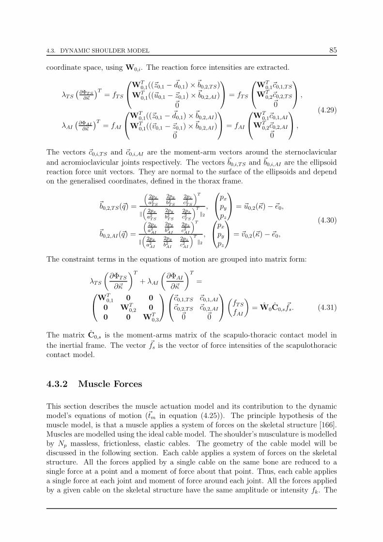
4.3. DYNAMIC SHOULDER MODEL 85
coordinate space, using W0,i. The reaction force intensities are extracted.
λTS(∂ΦTS
∂~κ
)T= fTS
WT0,1((~z0,1 − ~d0,1)×~b0,2,TS)
WT0,1((~u0,1 − ~z0,1)×~b0,2,AI)
~0
= fTS
WT0,1~c0,1,TS
WT0,2~c0,2,TS~0
,
λAI(∂ΦAI
∂~κ
)T= fAI
WT0,1((~z0,1 − ~d0,1)×~b0,2,AI)
WT0,1((~v0,1 − ~z0,1)×~b0,2,AI)
~0
= fAI
WT0,1~c0,1,AI
WT0,2~c0,2,AI~0
,
(4.29)
The vectors ~c0,i,TS and ~c0,i,AI are the moment-arm vectors around the sternoclavicular
and acromioclavicular joints respectively. The vectors ~b0,i,TS and ~b0,i,AI are the ellipsoidreaction force unit vectors. They are normal to the surface of the ellipsoids and dependon the generalised coordinates, defined in the thorax frame.
~b0,2,TS(~q) =
(
2pxa2TS
2pyb2TS
2pzc2TS
)T
‖
(
2pxa2TS
2pyb2TS
2pzc2TS
)T
‖2
,
pxpypz
= ~u0,2(~κ)− ~e0,
~b0,2,AI(~q) =
(
2pxa2AI
2pyb2AI
2pzc2AI
)T
‖
(
2pxa2AI
2pyb2AI
2pzc2AI
)T
‖2
,
pxpypz
= ~v0,2(~κ)− ~e0,
(4.30)
The constraint terms in the equations of motion are grouped into matrix form:
λTS
(∂ΦTS∂~κ
)T
+ λAI
(∂ΦAI∂~κ
)T
=
WT0,1 0 0
0 WT0,2 0
0 0 WT0,3
~c0,1,TS ~c0,1,AI~c0,2,TS ~c0,2,AI~0 ~0
(fTSfAI
)
= W0C0,s~fs. (4.31)
The matrix C0,s is the moment-arms matrix of the scapulo-thoracic contact model in
the inertial frame. The vector ~fs is the vector of force intensities of the scapulothoraciccontact model.
4.3.2 Muscle Forces
This section describes the muscle actuation model and its contribution to the dynamicmodel’s equations of motion (~tm in equation (4.25)). The principle hypothesis of themuscle model, is that a muscle applies a system of forces on the skeletal structure [166].Muscles are modelled using the ideal cable model. The shoulder’s musculature is modelledby Np massless, frictionless, elastic cables. The geometry of the cable model will bediscussed in the following section. Each cable applies a system of forces on the skeletalstructure. All the forces applied by a single cable on the same bone are reduced to asingle force at a point and a moment of force about that point. Thus, each cable appliesa single force at each joint and moment of force around each joint. All the forces appliedby a given cable on the skeletal structure have the same amplitude or intensity fk. The

86 4.3. DYNAMIC SHOULDER MODEL
forces and moments of force can be zero depending on the muscle. For instance, muscleswhich do not span the GH joint create no force and no moment of force about that joint.Forces applied to the clavicle are reduced to the centre of the SC joint. Forces applied tothe scapula are reduced to the centre of the AC joint. Forces applied to the humerus arereduced to the centre of the GH joint.
For a model with Np muscle segments, the total force and moment of force at eachjoint in the inertial reference frame R0 is defined by:
~f0,i =
Np∑
k=1
~f0,i,k, i = 1, 2, 3, (4.32)
~t0,i =
Np∑
k=1
~y0,i,k × ~f0,i,k =
Np∑
j=1
(
~y0,i,k ×~b0,i,k)
fk =
Np∑
j=1
~c0,i,kfk = C0,i~f. (4.33)
where the terms in these expressions are defined as:
• ~f0,i,k: resulting force of muscle k applied to body Bi in R0,
• ~y0,i,k: force system reduction vector for muscle k and body i in R0,
• ~c0,i,k = ~y0,i,k ×~b0,i,k: moment-arms of cable k and joint i in R0.
• C0,i: matrix of moment-arms of joint i in R0.
• ~f : Np × 1 total vector of muscle force intensities.
The equations of motion are in terms of rotational coordinates. Therefore, the musclecontribution to the equations of motion is from the resulting moments of force. Theresulting moment of force vectors ~t0,i are transformed to obtain the generalised momentof force vector ~tm, using the method described in chapter 3 section 3.6.4. The generalisedmoment of force is defined by
~tm =
WT0,1 0 0
0 WT0,2 0
0 0 WT0,3
~t0,1~t0,2~t0,3
= W0
C0,i~f
C0,2~f
C0,3~f
= W0C0
~f. (4.34)
C0 is the 9 × Np matrix of moment-arms dependent on the configuration of the model.Its computation will be discussed in detail in chapter 7. The expression (4.34) defines amap between the muscle force intensities and the generalised moments of force will bereferred to as the torque-force map.
The muscle-force contribution to the dynamic model’s equations of motion (4.25)-(4.27) is defined in terms of the force intensities using the torque-force map.
∂2L∂~κ2
~κ+∂2L∂~κ∂~κ
~κ− ∂L∂~κ
= W0C0~f + W0C0,s
~fs. (4.35)

4.3. DYNAMIC SHOULDER MODEL 87
Muscles can only pull the skeletal structure. As they contract, they pull on the bones towhich they are attached. This effect is included in the muscle force model by imposingbounds on the muscle-force intensities. A muscle’s force must be positive or zero withan upper limit given by the muscle’s maximum isometric strength (cf. chapter 2, section2.2).
~0 ≤ ~f ≤ ~fmax. (4.36)
The values used to implement these bounds were taken from VHP kinematic shouldermodel [76].
4.3.3 Muscle Cable Model
Geometrically, a muscle is an elongated volume between two points, the origin and inser-tion. The volume is filled with parallel fibres which go from origin to insertion. The cablemodel represents a particular fibre called the centroid line. The centroid line representsthe fibre which passes through the centre of the volume and therefore the centre of thevolume’s cross-sections.
Pi
Pi
Sj
Sj
Underlying Muscle
Cylinder Constraint ≡ Underlying muscle constraint Vi
Vi
Vj
Vj
Centroid line
Qk
Qk
Tk
Tk
Ri
Rk Ri
Figure 4.5: Illustration of the centroid line approach to muscle modelling as described insection 4.3.3. The underlying muscle is represented by a cylinder.
Once the centroid line is defined for the anatomical muscle, using MRI scans of themusculature, the geometric cable model is defined. The model is defined such that thecable follows the centroid line as closely as possible. To start, the cable is attachedat two points representing the origin Pi and insertion Sj which are fixed in the bonereference frames Ri and Rj respectively (Fig. 4.5). The centroid line of the anatomicalmuscle curves as the muscle passes over other anatomical structures. In the model,smooth geometric surfaces are inserted into the model to force the cable to curve as theanatomical centroid line does. The surfaces are spheres, cylinders, or cylinders with halfspheres at one end. For certain muscles, up to two extra fixed via points Vi and Vj areadded to force the cable to always pass through the point. These points are near theorigin and insertion points and are defined in the same reference frame. As the cablepasses over the surface, two points are defined which are the initial contact point Qk
and final contact point Tk with the surface. The points are defined in the same frameas the surface itself Rk. This construction of the cable model is the called the obstacle

88 4.3. DYNAMIC SHOULDER MODEL
set method and was initially developed for the VHP kinematic shoulder model [75]. Theapproach of modelling the muscle’s centroid line was first used in a model of the hip [108].
For the shoulder model, there are 16 anatomical muscles actuating the shoulder di-vided into 28 parts using the guide lines set fourth in [197] (cf. Appendix C for details).Thus, the shoulder model presented in this chapter uses at least 28 cables to model themusculature. A method of adding more cables is defined by parameterising the muscle’scentroid plane. A muscle’s centroid line passes through the centre of the muscle’s vol-ume. The muscle’s centroid plane cuts the muscle in half longitudinally and containsthe centroid line. The centroid plane defines a line at the muscle’s origin and insertion.The number of cables is modulated by parameterising these two lines using a third orderspline. The splines are constructed using three anchor points. The middle points are thecentroid line origins and insertions (Fig. 4.6).
Sj,s
Sj,m ≡ Sj,2Sj,f
Pi,s
Pi,m ≡ Pj,2Pi,f
Centroid Cable
Sj,1
Sj,3
Pi,1
Pi,3Vi,1
Vi,m ≡ Vi,2
Vi,3
Vi,s
Vi,f
12 3
Ri
Multi-cable model: Spline Construction:
Pi,s
Pi,m
Pi,f
Pi,k
~pi,s
~pi,m
~pi,f
~pi,k(µ)
Figure 4.6: (a) Illustration of a muscle’s centroid represented by three cables. (b) Illus-tration of the 3rd order spline parameterisation as described in section 4.3.3.
To illustrate the spline construction, consider the origin of a muscle which has beenidentified by a curved line. In the model, this line is parameterised using a 3rd orderspline with three anchor points Pi,s, Pi,m and Pi,f (Fig. 4.7). The spline is defined in thereference frame of the bone on which the muscle originates Ri. The location of any pointPi,k on the spline is defined using a single variable µ ∈ [0, 1]. The parameterisation isdefined by:
Pi,k(µ) : ~pi.k(µ) =
(µ3 µ2 µ 1
)S
~pi,s~pi,s~pi,m~pi,f
if 0 ≤ µ < 0.5
(µ3 µ2 µ 1
)S
~pi,s~pi,m~pi,f~pi,f
if 0.5 ≤ µ ≤ 1
,S =
−1
2
3
2−
3
2
1
2
1 5
22 −
1
2
−1
20 1
20
0 1 0 0
. (4.37)

4.4. REMARKS 89
The vectors ~pi,s, ~pi,m and ~pi,f are the points vectors of the points Pi,s, Pi,m and Pi,f in thelocal frame Ri. The matrix S is the spline coefficient matrix and is the same for everyspline. For muscle parts with multiple cables, the origin and insertion points of each cableare evenly distributed along the spline: µ = 1/(2 · Nb cables). This parameterisation isalso applied to the fixed via points (Fig. 4.6). If the number of cables is odd, there isa cable which represents the muscle’s centroid line. All the data necessary to constructthe geometry of the cable model was obtained through MRI scans of an adult male (cf.Appendix B).
The cable model defines the geometry of each cable. Once the geometry is known,pulley mechanics can be used to obtain the forces applied by each cable on the skeletalsystem. This information can then be used to compute the moment-arms and related theforces in the cables to the torques around the joints. This model does not state how muchforce is applied. The model simply gives the relation between the muscle force intensitiesand the joint torques. If there is force, this model transforms the force into torques atthe three joints.
4.4 Remarks
The musculoskeletal shoulder model presented in this chapter was developed for estimat-ing the forces within the muscles and in the glenohumeral joint. This is the model’spurpose that will be analysed in chapter 8. There are two other aspects to a model; itsstructure and numerical implementation. Many musculoskeletal models of the shoulderare presented in the context of their clinical application with a focus on the model’s clini-cal validity. While clinical validation is essential, the model’s mathematical structure andvalidity is also important. However, it seems there are few model oriented presentationsof musculoskeletal shoulder models, making their accurate reconstruction a challengingtask.
Figure 4.7: Pectoralis major (sternal muscle part, PMJs) modelled using one (left) and tensegments (right). Single cylinder wrapping constraint. The green and blue lines representthe muscle origin and insertion spline parameterisation.

90 4.4. REMARKS
The musculoskeletal shoulder model presented in this chapter contains a kinematicmodel of the skeletal structure. The bones are considered to be rigid bodies and thesynovial joints are modelled as ideal ball and socket joints parameterised by sphericalkinematic pairs. The model also considers the scapulothoracic contact, modelled byconstraining two points (TS, AI) to remain on the surface of two ellipsoids. The ellipsoidsrepresent the surface of the ribcage with an additional layer of muscle. The model’skinematics are completely characterised by the forward kinematic map.
ΞS : QS → WS ⊂ SE(3),
~q 7→ Ξ(~q) =(
~ǫ0,3(~q), ~Υ3
)
, with ~q = (~ΥT1 ,~ΥT
2 ,~ΥT
3 )T (4.38)
s.t. ΦTS(~Υ1, ~Υ2) = (~u0,2 − ~e0)TETS (~u0,2 − ~e0)− 1 = 0, (4.39)
ΦAI(~Υ1, ~Υ2) = (~v0,2 − ~e0)T EAI (~v0,2 − ~e0)− 1 = 0. (4.40)
The kinematic coordinates are the Euler and Bryan angles of the spherical kinematicpairs. There are nine coordinates total and the model has seven degrees of freedom giventhe two scapul-thoracic constraints.The dynamic model is constructed from the Euler-Lagrange equation. The kinematiccoordinates are defined as the generalised coordinates ~κ ≡ ~q. The dynamics are subjectto the scapulothoracic contact constraints (Eq. (4.39)-(4.40)). The muscles are modelledas massless, frictionless, perfectly elastic cables wrapping over the skeletal structure. Eachcable applies a system of forces to the skeletal structure modelled by a single matrix calledthe moment-arm matrix C0. The cable forces are also limited. Cables can only pull andtherefore the forces must be positive. Each cable’s ability to pull is limited by the muscle’smaximum isometric strength. This is the maximum force the muscle can produce whenit is at its optimal length (cf. chapter 3).
∂2L∂~κ2
~κ+∂2L∂~κ∂~κ
~κ− ∂L∂~κ
= W0C0~f + W0C0,s
~fs, (4.41)
s.t. ΦTS(~κ) = (~u0,2 − ~e0)TETS (~u0,2 − ~e0)− 1 = 0, (4.42)
ΦAI(~κ) = (~v0,2 − ~e0)T EAI (~v0,2 − ~e0)− 1 = 0, (4.43)
~0 ≤ ~f ≤ ~fmax. (4.44)
The musculoskeletal shoulder model presented in this chapter is most similar to thedynamic shoulder model constructed form the Visible Human Project (VHP) [76, 170].Both models differ mainly on the numerical data used to implement them and on thescapulothoracic contact model. The present model uses two ellipsoids while the VHPmodel uses a single ellipsoid. The model does not contain the entire upper limb or theconoid ligament constraint. The upper limb is considered to be outstretched.From a different perspective, the model presented in this chapter shares many similaritieswith models of cable-driven robots [29]. A cable-riven robot is a mechanism or system ofrigid bodies actuated by a network of cables [21, 80, 92, 178, 217, 220]. Models of suchsystems use the same hypothesis used to construct the musculoskeletal model presentedin this chapter. That is rigid bodies, ideal joints and ideal cables. This point is of interestbecause it means that theory developed for cable-driven robots can be applied to modelsof musculoskeletal systems. This will be used in chapter 7 to introduce a new conceptrelated to the muscle model.

4.5. CONCLUSIONS 91
4.5 Conclusions
This chapter presented a musculoskeletal model of the human shoulder constructed forthe purpose of estimating forces in the muscles and in the glenohumeral joint. The modelis constructed from three hypothesis. i. the bones are rigid bodies. ii. the synovialarticulations are ideal ball and socket joints. iii. the muscles are massless, frictionlesscables wrapping over the skeletal structure. The model also includes an ellipsoid model ofthe scapulothoracic contact. In comparison to other shoulder models, the present modelis most similar to the models constructed from the Visible Human Project. Furthermore,the model is shown to share similarities with models of cable-driven robots. Therefore, theoutlook of this thesis on musculoskeletal modelling in general is that the mathematicalstructure of musculoskeletal models is as important as their clinical validation. Thischapter presented many of the models mathematical details. The following chapterswill continue to discuss the different aspects of the shoulder model using the formalismintroduced in this chapter.

92 4.5. CONCLUSIONS

Chapter 5
Coordinated Redundancy
5.1 Introduction
The human shoulder is a system that is kinematically redundant and overactuated [36].The shoulder (humerus included) can move without moving the position of the elbow (tipof humerus) and multiple muscle activation patterns yield the same movement [66]. Tofunction properly, the shoulder uses coordination strategies to ensure that all parts worktogether harmoniously. Without the two characteristics of kinematic redundancy andoveractuation, the shoulder would not be nearly as performant as it is. The coordinatedmotion of the scapula and humerus, called the scapulo-humeral rhythm is an example ofthis coordination. As stated in chapter 2, the arm’s reachable space would be severelyreduced without the scapulo-humeral rhythm.
The general philosophy behind kinematic redundancy and overactuation is the dupli-cation of certain elements such that the tasks they perform are divided amongst them toenhance the system’s performance and flexibility [148]. This is called coordinated redun-dancy and is different from the usual definition of redundancy implying the duplicationof elements to increase reliability and not necessarily performance. Coordinated redun-dancy is used in systems design and robotics to increase performance and reduce costs.For example, in a milling machine multiple motors are used to drive the same positioningaxis (Fig. 5.1). One motor does the rough positioning of the part. Once the rough posi-tioning of the part is achieved, a second motor is used to precisely position the part. Thefirst motor drives the axis over its entire range of positions. The second motor drives theaxis around the rough position and has a small range of motion. This design enhances themilling machine’s precision and is cheaper. A single motor with higher performance char-acteristics is more expensive than two less performant motors. This is also an exampleof overactuation. Two motors are used when one could theoretically do the job.
Models of real systems that are kinematically redundant or overactuated or both,involve mathematical problems that are underdetermined. The primary characteristic ofunderdetermined mathematical problems is that there is an infinite number of solutions
93

94 5.2. KINEMATIC REDUNDANCY
[96]. Thus, a method of differentiating between the solutions is required, such that asolution can be selected that is best suited to the physics of the real system. There existmany methods of differentiating between solutions. Some consider the specifics of thesystem and others are more general and can be used for different systems sharing thesame mathematical structure. In general, a good solution is one taking advantage of themodel’s mathematics while considering the physics of the real system.
The goal of this chapter is to present kinematic redundancy and overactuation in anabstract mathematical context and to introduce possible coordination strategies withoutconsidering the specifics of the system. The notions of objective and task are also givenformal definitions. Kinematic redundancy is presented in section 5.2 with a formal defini-tion of a kinematically redundant mechanism. Overactuation is presented in section 5.3for a system where the equations of motion are described by the Euler-Lagrange equa-tion. Section 5.4 concludes the chapter with a presentation of using tasks for coordinatingredundancy.
Milling Machine Axes
Part to be milled
Tool
Motor 1
Rough positioning system
Precise positioning system
Motor 2
Figure 5.1: Illustration of coordinated redundancy in a milling machine as described insection 5.1.
5.2 Kinematic Redundancy
A kinematically redundant mechanism is informally defined as a mechanism with a num-ber of internal degrees of freedom that exceeds the number of degrees of freedom of theend-effector [148]. As stated in chapter 3, a mechanism is a rigid body model of a ma-chine where one body is fixed in the inertial frame. This body is called the carrier body.The purpose of a machine is to transmit motion and therefore force to a specific partof the machine called the end-effector. Motion is transmitted within a machine by theinteractions between bodies. Joints represent idealised mechanical models of the interac-tions and kinematic pairs represent mathematical parameterisations of the interactions.Kinematic pairs also impose holonomic skleronomic constraints on the bodies forming thejoint. This discussion is limited to systems subject to holonomic skleronomic constraints.Thus, a mechanism is a set of rigid bodies connected by kinematic pairs and subject toa certain number of constraints.

5.2. KINEMATIC REDUNDANCY 95
A kinematic chain is a set of rigid bodies connected together by kinematic pairs. Ifall the bodies are connected in series from carrier body to end-effector, the kinematicchain is open. An example is a serial robot manipulator (Fig. 5.2). A kinematic chainis closed if there are two serial chains with same initial and final bodies. The simplestclosed kinematic chain is two serial chains, joined together (not necessarily at the carrierbody and end-effector). A mechanism with more than two kinematic chains between twobodies is called a parallel mechanism. An example of a parallel mechanism is the Gough-Stewart platform. An important remark is that redundancy is not related to whethera kinematic chain is open or closed. Kinematic redundancy is defined by the numberof bodies and the number and types of connections. A Gough-Stewart platform is notkinematically redundant.
Machine (Serial Manipulator)
Mechanism
Carrier Body
End-effector
Connections
Bodies
Machine (Parallel Manipulator)
Mechanism
Carrier Body
End-effector
Figure 5.2: Illustrations of machines and their corresponding mechanisms as described insection 5.2 and chapter 3.
A kinematic model is a parameterisation of a mechanism’s geometric configurationand how it can change over time. Kinematics analyses the possible effects in terms ofmotion without considering the cause. The parameterisation is obtained by constructinga set of coordinates ~q completely defining the mechanism’s geometric configuration C atany given instant. Geometric configuration is understood as the position and orientationof each body Bi in the mechanism, defined by a Euclidean displacement with respect tothe inertial frame (cf. chapter 3).
X0,i ∈ Bi : ~x0,i = ~d0,i︸︷︷︸
Position
+ Ri,0~xi︸ ︷︷ ︸
Orientation
. (5.1)
A possible method of constructing the set of coordinates is to define coordinates for everykinematic pair along one of the kinematic chains between the carrier body and end-effector. If the set is incomplete, additional coordinates are defined until the remaining

96 5.2. KINEMATIC REDUNDANCY
kinematic pairs can be expressed as holonomic skleronomic constraints in terms of thecomplete set of kinematic coordinates. The selected kinematic chain between the carrierbody and end-effector is used to define the forward kinematic map which is then subjectto the constraints. The forward kinematic map of a mechanism with Nb bodies and Nk
kinematic pairs parameterised by Q coordinates and subject to Nc holonomic skleronomicconstraints is defined by:
Ξ : Q → W ,
~q 7→ Ξ(~q) = Ce = (~ǫT0,e, ~ΥTe )
T , with
(~ǫ0,e1
)
= He,0
(~ǫe1
)
(5.2)
s.t.
Φ1(~q) = 0,...ΦNc(~q) = 0.
(5.3)
The vector ~ǫ0,e is the end-effector’s position with respect to the carrier body and He,0 isthe 4×4 homogeneous transformation matrix. Q defines the coordinate or configurationspace and W defines the workspace. The workspace defines in what space the end-effectorcan move. The nature of the work space is dependent on the type of manipulator. Giventhat a rigid body has at most six degrees of freedom (dof), the work space is a subset ofone of the following possibilities.
• W ⊆ R: a linear manipulator (End-effector dof: De = 1)
• W ⊆ R2: a planar manipulator (dof: De = 2)
• W ⊆ R2 × SO(2): a planar manipulator with orientation (dof: De = 3)
• W ⊆ R3: spatial manipulator (dof: De = 3)
• W ⊆ R3 × SO(2): spatial manipulator with partial orientation (dof: De = 4)
• W ⊆ R3 × S2: spatial manipulator with partial orientation (dof: De = 5)
• W ⊆(R3 × SO(3)
)≡ SE(3): spatial manipulator with orientation (dof: De = 6)
The number of internal degrees of freedom of a mechanism is defined as Di = Q−Nc.Thus, a mechanism is kinematically redundant when Di > De. The number Dr = Di−De
is called the degree of redundancy. An equivalent formal definition is stated as follows.
Definition 12 (Kinematically Redundant Mechanism [148]). A mechanism consistingof Nb rigid bodies and Nk kinematic pairs, parameterised by Q coordinates subject to Nc
holonomic skleronomic constraints is kinematically redundant, when, for a fixed configu-ration Ce ∈ W of the end-effector, there exists an infinite number of joint configurations~q ∈ Q.
Given this definition of kinematic redundancy, a coordination strategy consists of find-ing for any fixed configuration Ce ∈ W of the end-effector, a solution ~q ∈ Q of the joint

5.3. OVERACTUATION 97
coordinates that satisfies the constraints. Furthermore, given the infinite number of so-lutions one can find a solution satisfying additional requirements. The greater the degreeof redundancy, the more additional requirements the solution can satisfy simultaneously.
The concepts discussed above are very machine inspired concepts. The notion of end-effector is a robotics oriented term. However, this discussion does have its meaning inthe context of biomechanics and musculoskeletal modelling. Indeed, the model presentedin chapter 4 is built as a multibody systems model. This type of model can be abstractlyseen as machine. Furthermore, the hand is a manipulator that we continuously use tointeract with out environment. Our hand is an end-effector in the same way a mechanicalgripper is the end-effector of a robotic machine.
5.3 Overactuation
Actuation is defined as to put into action. In a machine, the external forces make thedifferent links move. However, the term actuation is limited to the forces that can becontrolled. The torque generated by an electric motor is an actuation, the earth’s grav-itational pull is not. A machine can be fully actuated, underactuated or overactuated.A machine can also be simultaneously under and overactuated. Although this situationis not common, it is possible. Overactuation is to use more controlled forces than neces-sary. An overactuated mechanism has a number of controlled actuators that exceeds thenumber of internal degrees of freedom [159]. Fully actuated and underactuated machineshave respectively an equal number or less controlled actuators than internal degrees offreedom.
An actuator is a controlled element of a mechanism that applies a force and/or momentof force to the mechanism. The force and moment of force are function of a single variableui allowing the actuation to be controlled over time. The force in a muscle is controlledby its activation level. The force depends on other variables but is actively controlledby its neural activation level. Given that actuators generate forces in a machine, theyappear in the dynamic model of a mechanism relating the mechanism’s movement to theforces and moments of force that are applied to it. Consider the dynamic model of amechanism parameterised by a vector of Q generalised coordinates ~κ and subject to Nc
holonomic skleronomic constraints. The model is constructed using the Euler-Lagrangeequation. The generalised coordinates are defined as the kinematic coordinates from theprevious section: ~κ = ~q. The system has Na actuators. The Euler-Lagrange equation,with the lagragian augmented by the constraints is defined according to chapter 3 by:
d
dt
(
∂L∂~κ
)
− ∂L∂~κ
=
Na∑
i=1
~ti(ui), L = L+ ~Φ(~κ)T · ~λ. (5.4)
s.t. ~Φ(~κ) = ~0, Nc constraints. (5.5)
where ~ti(ui) is the generalised force associated to an actuator, parameterised by thevariable ui. The generalised actuator force is either a real force or a moment of force.

98 5.4. TASKS FOR COORDINATION STRATEGIES
The right-hand side of (5.4) is parameterised by the position, velocity and accelera-tions of the mechanism’s generalised coordinates. The set ~κ, ~κ, ~κ defines the mech-anism’s dynamic state. The vector ~u = (u1, . . . , uNa)
T ∈ RNa defines the mechanism’s
actuator state or input state. The degree of actuation of a mechanism is defined by thenumber of actuator variables Na. A mechanism is overactuated when Na > D = Q−Nc.An equivalent formal definition is stated below.
Definition 13 (Overactuated Mechanism [148]). A mechanism consisting of a numberof bodies and kinematic pairs, parameterised by n coordinates subject to p holonomic
skleronomic constraints is overactuated, when, for a fixed dynamic state ~κ, ˙~κ, ¨~κ of themechanism, there exists an infinite number actuator states ~u ∈ R
k.
Given this definition of overactuation, a coordination strategy consists of finding a
solution ~u ∈ Rk of the input states for any dynamic state ~κ, ˙~κ, ¨~κ of the mechanism.
Just like kinematic redundancy, if the mechanism is highly overactuated a solution canbe found satisfying multiple criteria.
5.4 Tasks for Coordination Strategies
In both kinematic redundancy and overactuation, a coordination strategy consists offinding a solution to a mathematically underdetermined problem. In this presentation, amathematically underdetermined problem is defined by a set of Ne smooth scalar equa-tions, function of Nq > Ne variables. The equations are grouped to define a map.
χ(~υ) : Rq ⊂ RNq → Re ⊂ R
Ne ,
~υ 7→χ1(~υ) = ε1...χNe(~υ) = εNe
χ(~υ) = ~ε, (5.6)
The map is surjective. There are more equations than variables and therefore there isan infinite number of vectors ~υ for a given vector ~ε. A coordination strategy for such aproblem is to find a parameterisation of the variables υj in terms of the parameters εi.
~υ = ~υ(~ε). (5.7)
The problem can be solved for a continous time-dependent parameterisation of ~ε(t),t ∈ [t0, tf ]. For every point ~ε(ti) along the path, there are an infinite number of solutions~υa(ti), ~υb(ti), ~υc(ti), . . . (Fig. 5.3). Thus, for every path ~ε(t) there are an infinite numberof paths ~υa(t), ~υb(t), ~υc(t), . . . , defined by the collection of points for all t ∈ [t0, tf ].
All the solutions ~υa(ti), ~υb(ti), ~υc(ti), . . . for a given point ~ε(ti) define a local man-ifold Ω~ε(ti) within Rq. For a given path ~ε(t), all the paths ~υa(t), ~υb(t), ~υc(t), . . . passthrough the local manifolds Ω~ε(t) at a point, respectively ~υa(ti), ~υb(ti), ~υc(ti), . . . . Thisis important, the local manifolds Ω~ε(ti) are normal to each other and do not intersect.

5.4. TASKS FOR COORDINATION STRATEGIES 99
RNq
RNe
χ
Rq
Re
~ε(t0)
~υa(t0)
~ε(ti)
~υa(ti)
~ε(tf )
~υa(tf )
~ε(t) = χ(~υa(t)) = χ(~υb(t)) = χ(~υc(t)), t ∈ [t0, tf ]~υa(t), t ∈ [t0, tf ]
~υb(t), t ∈ [t0, tf ]
~υc(t), t ∈ [t0, tf ]
η(tf ) ∈ Ω~ε(tf )
η(t0) ∈ Ω~ε(t0)
η(ti) ∈ Ω~ε(ti)
Figure 5.3: Illustrations of local manifolds Ω~ε(ti) in coordinated redundancy as describedin section 5.4.
The collection of local manifolds defines the redundant manifold Ω~ε(t). A coordinationstrategy is to find a path ~υ(t) on the redundant manifold, given ~ε(t).
The solutions are obtained by differentiation of the solution set Rq using a task [148].The primary task is ~ε(t) because it differentiates the redundant manifold from withinRq. The redundant manifold is a subset of Rq and contains all possible solutions giventhe primary task. The primary task reduces the search for a solution to a subset ofRq but does not define a specific solution. Multiple tasks can be used to obtain a finerdifferentiation of the solution set. The resulting solution will be a compromise betweenthe individual task specific solutions. This is defined as constructive coordination [148].
There are multiple methods of finding a specific solution. A first method which appliesto almost all underdetermined problems is to use static optimisation. A secondary taskis defined using a cost function of the variables ~υ. The primary task is discretised intoNt points: ~ε(t), t ∈ t0, t1, . . . , tNt = tf. A static optimisation problem or nonlinearprogram (NLP) is defined for each point, where the underdetermined map defines anequality constraint. The solution must also belong to the coordinate set Rq.
min~υ(tk)
Γ(~υ(tk)), ~υ(tk) ∈ Rq, (5.8)
s.t. χ(~υ(tk)) = ~ε(tk), (5.9)
A second method is to use an extension of the map χ. Extra equations are added such as toreduce the degree of underdeterminacy and thereby extend the map. Underdeterminacycannot be fully eliminated because there is no guarantee a solution will exist. However, byadding additional equations, the search for a solution can be made easier. An optimisation

100 5.4. TASKS FOR COORDINATION STRATEGIES
problem is defined using the extended map. The extension defines additional tasks.
min~υ(tk)
Γ(~υ(tk)), ~υ(tk) ∈ Rq, (5.10)
s.t. χ(~υ(tk)) = ~ε(tk), (5.11)
~Φ(~υ(tk)) = ~0, (5.12)
A third method is to define a reduced set of coordinates ~υ that is better suited to themathematical structure of the problem. This method is similar to the idea of usinggeneralised coordinates in analytical mechanics (cf. chapter 3). In analytical mechan-ics, generalised coordinates are defined that are better suited to the mathematics of thedynamic model. These coordinates are constructed from equality constraints that arethereby eliminated. In the context of underdetermined problems, the idea is the same. Areduced set of coordinates is constructed using the mathematical structure of the redun-dant manifold Ω~ε(t). If the number of coordinates still exceeds the number of equations,some form of optimisation will be needed. However, the problem will be easier, giventhat there are less optimisation variables.
These three methods are not the only solutions to solving underdeterminacy. Thereexist a number of other methods not discussed here. The following paragraphs redefinethe problems of kinematic redundancy and overactuation using the definitions of taskand redundancy manifold.
In kinematic redundancy, the primary task is a specific trajectory of the end-effectorCe(t), t ∈ [0, T ], defined with respect to the internal reference frame. The problem is tofind the kinematic coordinates ~q ≡ ~υ. If the static optimisation method is used, the costfunction could be for instance, the error between the kinematic coordinates of the modeland a set of measured coordinates obtained from the real system ~qm(tk), tk ∈ [0, T ]. Thecoordination problem is solved at each time step tk for which a measurement was taken.
min~q(tk)
Γ(~q(tk) = ‖~qm(tk)− ~q(tk)‖2, ~q(tk) ∈ Q, (5.13)
s.t. Ξ(~q(tk)) = Ce(tk) = Ξ(~qm(tk)), (5.14)
Φ1(~q) = 0,...ΦNc(~q) = 0
. (5.15)
The redundant manifold ΩCe(t) is comprised of all the local manifolds ΩCe(ti). The localmanifolds are called self motions. The mechanism moves without changing the configu-ration of the end-effector.
In overactuation, the primary task is a dynamic behaviour defined by a time-dependentparameterisation of the dynamic state: ~κ(t), ~κ(t), ~κ(t), t ∈ [0, T ]. The problem is to findthe input variables ~u ≡ ~υ. If the static optimisation method is used, the cost functioncould be for instance, the inputs using the least amount of energy. A static optimisationis defined for every discrete instant of the primary task and the input variables are further

5.4. TASKS FOR COORDINATION STRATEGIES 101
constrained by the real systems physical limitations.
min~u(tk)
Γ(~u(tk) =1
2
Na∑
j=1
uj(tk), ~u(tk) ∈ RNa , (5.16)
s.t.
(
d
dt
(
∂L∂~κ
)
− ∂L∂~κ
)
~κ(tk),~κ(tk),~κ(tk)
=
Na∑
j=1
~tj(uj(tk)), (5.17)
~umin ≤ ~u(tk) ≤ ~umax. (5.18)
The redundant manifold Ωu is the set of inputs that can be applied to the system withoutchanging the dynamic state.
As stated in the introduction, the human shoulder is a system that is both kinemati-cally redundant and overactuated. There are seven degrees of freedom while the humerushas six and there are p > 28 muscle forces. Overactuation coordination strategies requirethe dynamic state of the model. If a system is both kinematically redundant and overac-tuated, one must choose to either use two independent coordination strategies or to usea combined strategy. Combined strategies are in general more complex. An example of acombined strategy is optimal control [66, 165]. Therefore, this thesis proposes to use twostrategies that are solved successively. Chapter 6 discusses the coordination strategy forthe kinematic redundancy problem and chapter 7 discusses the coordination strategy forthe overactuation problem.

102 5.4. TASKS FOR COORDINATION STRATEGIES

Chapter 6
Shoulder Kinematic Redundancy
Coordination
6.1 Introduction
Human motion or kinematics is defined as the combined motion of all the bones in theskeletal system. Its synthesis for the purpose of simulation in a model is a challenging taskbecause the skeletal system is covered by a layer of skin and muscle. Human kinematicsare not directly observable [42]. One can only estimate human motion and a possibletechnique is the palpation of markers on the skin [211].The synthesis of human movement is composed of two parts: measurement based de-scription and model based parameterisation. The description of human motion is thedescription based on measurements of each bone’s individual movement relative to theother and with respect to a fixed frame [113, 143, 147]. The parameterisation of humanmotion is the use of mathematical models called kinematic pairs and chains to reproducethe description [50, 61, 104]. The models are constructed under the hypothesis that phys-iological articulations behave like ideal mechanical joints [61, 62]. The use of kinematicpairs to model joints provides a natural parameterisation of joint motion using joint co-ordinates. This chapter focuses on the parametrisation of shoulder motion that has anadditional challenge. The skeletal structure of the human shoulder is a kinematicallyredundant system. Multiple sets of joint coordinates produce the same elbow position.
Given the hypothesis of ideal mechanical joints, constructing kinematic shoulder mod-els is straightforward. Many different models have been developed that can be dividedinto two types. The first type includes the three anatomical joints and model the systemas an open kinematic chain [54, 63, 101, 103, 114]. The second type of kinematic shouldermodel includes the three joints and a model of the scapulothoracic contact, defining thesystem as a closed kinematic chain [74, 194]. Open kinematic chain models are easier touse because all the coordinates are independent but are less accurate because they donot consider the scapula being held against the thoracic cage by the muscles [58]. Closedkinematic chain models are more accurate but more difficult to use because the coordi-
103
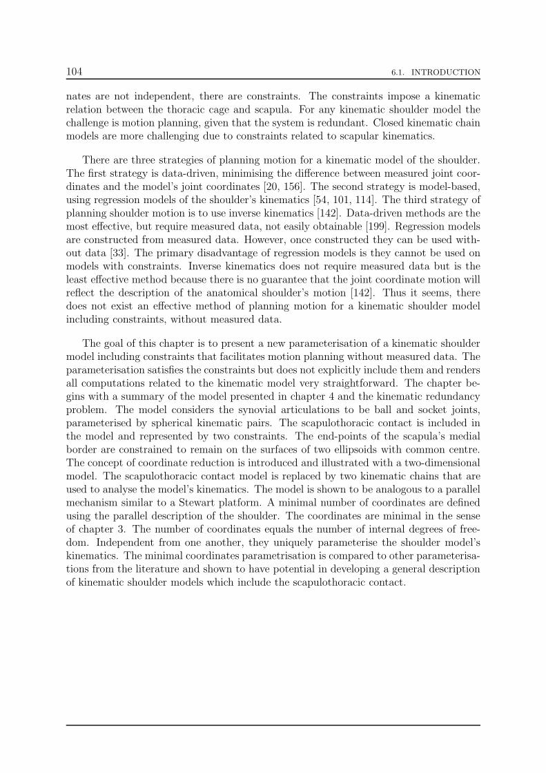
104 6.1. INTRODUCTION
nates are not independent, there are constraints. The constraints impose a kinematicrelation between the thoracic cage and scapula. For any kinematic shoulder model thechallenge is motion planning, given that the system is redundant. Closed kinematic chainmodels are more challenging due to constraints related to scapular kinematics.
There are three strategies of planning motion for a kinematic model of the shoulder.The first strategy is data-driven, minimising the difference between measured joint coor-dinates and the model’s joint coordinates [20, 156]. The second strategy is model-based,using regression models of the shoulder’s kinematics [54, 101, 114]. The third strategy ofplanning shoulder motion is to use inverse kinematics [142]. Data-driven methods are themost effective, but require measured data, not easily obtainable [199]. Regression modelsare constructed from measured data. However, once constructed they can be used with-out data [33]. The primary disadvantage of regression models is they cannot be used onmodels with constraints. Inverse kinematics does not require measured data but is theleast effective method because there is no guarantee that the joint coordinate motion willreflect the description of the anatomical shoulder’s motion [142]. Thus it seems, theredoes not exist an effective method of planning motion for a kinematic shoulder modelincluding constraints, without measured data.
The goal of this chapter is to present a new parameterisation of a kinematic shouldermodel including constraints that facilitates motion planning without measured data. Theparameterisation satisfies the constraints but does not explicitly include them and rendersall computations related to the kinematic model very straightforward. The chapter be-gins with a summary of the model presented in chapter 4 and the kinematic redundancyproblem. The model considers the synovial articulations to be ball and socket joints,parameterised by spherical kinematic pairs. The scapulothoracic contact is included inthe model and represented by two constraints. The end-points of the scapula’s medialborder are constrained to remain on the surfaces of two ellipsoids with common centre.The concept of coordinate reduction is introduced and illustrated with a two-dimensionalmodel. The scapulothoracic contact model is replaced by two kinematic chains that areused to analyse the model’s kinematics. The model is shown to be analogous to a parallelmechanism similar to a Stewart platform. A minimal number of coordinates are definedusing the parallel description of the shoulder. The coordinates are minimal in the senseof chapter 3. The number of coordinates equals the number of internal degrees of free-dom. Independent from one another, they uniquely parameterise the shoulder model’skinematics. The minimal coordinates parametrisation is compared to other parameterisa-tions from the literature and shown to have potential in developing a general descriptionof kinematic shoulder models which include the scapulothoracic contact.

6.2. MINIMAL COORDINATES FOR COORDINATION 105
6.2 Minimal Coordinates for Coordination
6.2.1 Shoulder Kinematic Redundancy Coordination
In chapter 4, a kinematic model of the shoulder’s skeletal structure is presented. Themodel is constructed on the hypotheses that all bones are rigid bodies and that all thesynovial articulations behave like ideal ball and socket joints. The joints are parame-terised using spherical kinematic pairs. The scapulothoracic contact is modelled usingtwo holonomic skleronomic constraints that keep the points TS and AI on the surfaceof two ellipsoids with identical centres E (cf. chapter 2 for anatomical references). Theellipsoids represent the thoracic cage with the additional layer of muscle between the ribsand the under side of the scapula. The constraints are equivalent to two spherical sliderkinematic pairs between the scapula and ribcage. A body gliding on a surface through apunctual contact is a spherical slider kinematic pair (cf. chapter 3).
R0
R1
R1
R2
R2
R3
R3
ψ1
ϑ1
ϕ1
ψ2
ϑ2
ϕ2
ψ3
ϑ3
ϕ3
Joint Coordinate Definitions:
IJ
IJ
PX
T8
T8
C7C7
SCAC
AC
AA AA
TS
AIGH
GH
HU
EL
EM
Figure 6.1: Illustration of the bony landmarks, reference frames and joint coordinates asdefined in section 6.2.1. Image created using ZygoteBodyTM zygotebody.com.
Each bone is attributed a reference system located at the centre of a joint. The bonereference frames are defined according to the ISB guide lines [214]. The thorax is thecarrier body and its reference frame is defined as the inertial frame R0 (cf. chapter 4).The frame is located at the point IJ (Fig. 6.1). The clavicle’s reference frame R1 islocated as the centre of the sternoclavicular joint SC. The scapula’s reference frameR2 is located at the centre of the acromioclavicular joint AC. The humeral referenceframe R3 is located at the centre of the glenohumeral joint R3. The reference frames are

106 6.2. MINIMAL COORDINATES FOR COORDINATION
differentiated using subindexes. 0: thorax frame, 1: clavicle frame, 2: scapula frame, 3:humerus frame.
The model’s configuration is parameterised by a set of nine angular coordinatesgrouped into subsets of three. The first three coordinates ~Υ1 = (ψ1, ϑ1, ϕ1)
T are Bryanangles parameterising the configuration of the sternoclavicular joint (SC) and therebythe clavicle’s configuration with respect to the thorax frame. The next three coordinates~Υ2 = (ψ2, ϑ2, ϕ2)
T are Bryan angles parameterising the configuration of the acromio-clavicular joint (AC) and scapula with respect to the thorax. The Bryan angle rotation
sequence is defined as XYZ. The last three coordinates ~Υ3 = (ψ3, ϑ3, ϕ3)T are Euler an-
gles parameterising the configuration of the glenohumeral joint (GH) and humerus withrespect to the thorax. The Euler angle rotation sequence is ZYZ. Thus, the vector ofkinematic coordinates is defined by:
~q =(~ΥT
1~ΥT
2~ΥT
3
)T=(ψ1 ϑ1 ϕ1 ψ2 ϑ2 ϕ2 ψ3 ϑ3 ϕ3
)T. (6.1)
The end-effector is defined as the humerus. Its configuration Ce is defined as the positionof the humeroulnar joint HU0,3 and the orientation of the humerus with respect to thethorax frame (cf. chapter 2 for conventions on notation).
Ce = (~ǫT0,3,~ΥT
3 )T , (6.2)
HU0,3 : ~ǫ0,3 = ~d0,1 +R1,0~z1 +R2,0~z2 +R3,0~ǫ3. (6.3)
~d0,1: vector from IJ to SC in R0. ~z1: vector from SC to AC in R1. ~z2: vector fromAC to GH in R2. ~ǫ3: vector from GH to HU in R3. The conventions on the rotationmatrices are defined in chapter 4.
The forward kinematic map is defined as the function which maps the joint coordinatesto the spatial configuration of the humerus (position and orientation). The map is subjectto the constraints modelling the scapulothoracic contact.
ΞS : QS → WS,
~q 7→ ΞS(~q) = Ce = (~ǫT0,3,~ΥT
3 )T , (6.4)
s.t. ΦTS(~q) = (~u0,2 − ~e0)TETS (~u0,2 − ~e0)− 1 = 0, (6.5)
ΦAI(~q) = (~v0,2 − ~e0)T EAI (~v0,2 − ~e0)− 1 = 0. (6.6)
The matrices ETS and EAI are the ellipsoid quadric matrices. The vectors ~u0,2 and ~v0,2are the point vectors of TS and AI respectively, in the inertial frame R0. The vector ~e0is the point vector of the common centre of the ellipsoids.
As stated in chapter 5, this kinematic shoulder model is kinematically redundant andthe map is underdetermined. For a fixed configuration of the humerus Ce ∈ WS, there isan infinite number of kinematic coordinates sets ~q ∈ QS. Furthermore, it was also statedin chapter 5 that a possible solution to the problem is to minimise the error between themodel’s coordinates ~q(tk) and the measured values of the coordinates ~qm(tk) at discreteinstances of a motion tk ∈ [0, T ] (the subindex m indicates measured).

6.2. MINIMAL COORDINATES FOR COORDINATION 107replacemen
TS Ellipsoid Gliding Surface R0
IJ
AI Ellipsoid Gliding Surface
ACACACSC
AC
GH
HU
TS
TS
AI
AI
AAAA
Scapulothoracic joint : ST
Figure 6.2: Diagram of the shoulder’s kinematic model, as defined in chapter 4. Imagecreated using ZygoteBodyTM zygotebody.com.
Consider a movement was measured on a real shoulder, for instance abduction in thescapular plane (cf. chapter 2). Markers were placed on the body of a subject at thelocations of bony landmarks and measurements of the marker locations were taken atN different instants tk ∈ t0, . . . , tN during the motion. The palpated marker positionswhere then used to estimate the position of the bony landmarks [56]. The estimatedbony landmark positions were used to reconstruct the bone reference frames and theEuler and Bryan angles were extracted [56, 58, 199]. The result is a set of measuredcoordinate vectors: ~qm(t0), ~qm(t1), . . . , ~qm(tk), . . . , ~qm(tN). As defined in chapter 5, aset of model coordinate vectors ~q(t0), ~q(t1), . . . , ~q(tk), . . . , ~q(tN) can be found by solvingthe following static optimisation problem at every instant tk of the motion.
min~q(tk)
Γ(~q(tk)) =1
2‖~qm(tk)− ~q(tk)‖2 =
1
2
9∑
i=1
(qm,i(tk)− qi(tk))2, ~q(tk) ∈ QS, (6.7)
s.t. ΞS(~q(tk))− ΞS(~qm(tk)) = ~0, (6.8)
ΦTS(~q(tk)) = 0, (6.9)
ΦAI(~q(tk)) = 0. (6.10)
This problem defines a kinematic coordination strategy as presented in chapter 5. Theapproach is straightforward but requires the availability of measured data. If the problemis unconstrained, an optimisation problem is unnecessary. One could directly impose theequality between the model’s coordinates and the measured coordinates.

108 6.2. MINIMAL COORDINATES FOR COORDINATION
6.2.2 Manifolds and Coordinate Reduction
This section introduces the idea that a different parameterisation of the coordinate spaceQS can eliminate the constraints in the kinematic coordination strategy. Furthermore,the parameterisation makes all computational operations related to the model’s kinematiccoordination straightforward. The parameterisation is constructed by taking advantageof the mathematical structure of the coordinate space QS.
The forward kinematic map and the two scapulothoracic constraints are assumedto be smooth or C∞ functions of the joint coordinates. Under these assumptions, thecoordinate space is a compact smooth manifold. Indeed, the nine kinematic coordinatesdefine charts φi,S from subsets of R3 to SO(3) in sets of three.
φi,S : [−π, π]× [−π, π]× [−π, π] → SO(3), i = 1, 2, 3,
(ψi, ϑi, ϕi) 7→ φi,S(ψi, ϑi, ϕi) = Ri,0. (6.11)
The coordinate space QS is a subset of the space (SO(3))3 = SO(3)× SO(3)× SO(3).The elements of the coordinate space are the rotation matrices (R1,0,R2,0,R3,0) ∈ QS ⊂(SO(3))3. For a given task of the end-effector, the redundant manifold Ω~ǫ(t) is a subspaceof QS (cf. chapter 5). The redundant manifold contains all the self motions associatedto the task.The group SO(3) is isomorphic or identical to the space of rotations in R
3. It is a Liegroup (group with a natural manifold structure), diffeomorphic to the real projectivespace RP
3, a compact smooth or C∞-manifold. This implies that SO(3) is a compactC∞-manifold which implies that (SO(3))3 is also a compact C∞-manifold. The coordinatespace of the kinematic shoulder model presented in chapter 4 and summarised in section6.2.1 is a compact C∞-manifold of dimension seven. There are nine coordinates subjectto smooth equality constraints.The image space or work space WS is a subset of SE(3) = R
3 × SO(3). SE(3) is notcompact (R3 is not compact) but is a smooth manifold. However, given that QS iscompact and that ΞS is smooth, the work space is also compact. The image of a compactspace through a smooth map is also compact. The humerus works in a compact subset ofR
3. Thus, the coordinate space QS and work space WS of the shoulder’s forward kinematicmaps are compact C∞-manifolds of dimensions seven and six respectively, having theparticular mathematical structure of locally looking like subsets of the Eulcidean spaceof the same respective dimension.
A smooth or C∞-manifold is a particular type of differentiable manifold. Differentiablemanifolds are found in numerous engineering problems and involve Ck functions withk ≥ 1. The constraints of an optimisation problem can define a differentiable manifold,under certain assumptions on the type of constraints. The domain space and imagespace of the kinematic map of a robot manipulator can involve differentiable manifoldsas illustrated previously. Dynamic systems can evolve on differentiable manifolds. Thus,differentiable manifolds are important from an engineering point of view but are notalways apparent. A simple definition of a differentiable manifold is that it is a subset ofRn of dimension k that locally ”looks” exactly like R
k. This can also be understood as
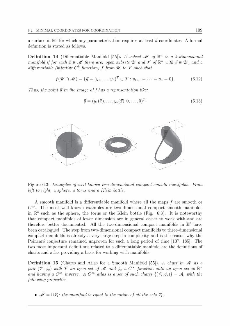
6.2. MINIMAL COORDINATES FOR COORDINATION 109
a surface in Rn for which any parameterisation requires at least k coordinates. A formal
definition is stated as follows.
Definition 14 (Differentiable Manifold [55]). A subset M of Rn is a k-dimensional
manifold if for each ~x ∈ M there are: open subsets U and V of Rn with ~x ∈ U , and adifferentiable (bijective Ck function) f from U to V such that
f(U ∩ M ) = ~y = (y1, . . . , yn)T ∈ V : yk+1 = · · · = yn = 0. (6.12)
Thus, the point ~y in the image of f has a representation like:
~y = (y1(~x), . . . , yk(~x), 0, . . . , 0)T . (6.13)
Figure 6.3: Examples of well known two-dimensional compact smooth manifolds. Fromleft to right, a sphere, a torus and a Klein bottle.
A smooth manifold is a differentiable manifold where all the maps f are smooth orC∞. The most well known examples are two-dimensional compact smooth manifoldsin R
3 such as the sphere, the torus or the Klein bottle (Fig. 6.3). It is noteworthythat compact manifolds of lower dimension are in general easier to work with and aretherefore better documented. All the two-dimensional compact manifolds in R
3 havebeen catalogued. The step from two-dimensional compact manifolds to three-dimensionalcompact manifolds is already a very large step in complexity and is the reason why thePoincare conjecture remained unproven for such a long period of time [137, 185]. Thetwo most important definitions related to a differentiable manifold are the definitions ofcharts and atlas providing a basis for working with manifolds.
Definition 15 (Charts and Atlas for a Smooth Manifold [55]). A chart in M as apair (V , φv) with V an open set of M and φv a C∞ function onto an open set in R
k
and having a C∞ inverse. A C∞ atlas is a set of such charts (Vi, φi) = A, with thefollowing properties.
• M = ∪Vi: the manifold is equal to the union of all the sets Vi,

110 6.2. MINIMAL COORDINATES FOR COORDINATION
M
U
V
φu
φv
φuv a diffeomorphism
φu(U )
φv(V )
φu(U ∩ V )
φv(U ∩ V )
Rk
Rk
Figure 6.4: Diagram of two charts of a C∞ atlas on a differentiable (smooth) manifoldM in R
n of dimension Rk as described in section 6.2.2, definition 4.
• If (Vu, φu) and (Vv, φv) are in A and Vv ∩ Vu 6= ∅, then
φvu = φu φ−1v : φv(Vv ∩ Vu) → φu(Vv ∩ Vu)
is a C∞ diffeomorphism (bijective C∞ function)
An intuitive example of charts and atlases on a smooth manifold, is the maps of theEarth that are flat. They are parameterised in R
2 but they map at part of the Earthwhich is a sphere in R
3. Each map defines a chart and all the maps form an atlas ofthe Earth’s spherical manifold. Just like maps of the Earth, charts and atlases are notunique.
A k-dimensional, differentiable manifold in Rn can be parameterised by k ≤ Q ≤ n
coordinates. In general, each coordinate belongs to a subset of R and the vector of coor-dinates belongs to a subset of RQ. The most attractive description is to use k coordinatesbecause they are all independent. Furthermore, the Euclidean space Rk is a vector spacethat is very easy to work with for any finite k. Given that the charts from the previousdefinition are all Ck and invertible, all operations related to the manifold can be carriedout in R
k and then mapped onto the manifold using the inverse chart. The independentdirections related to each variable are orthogonal and straight. It is the charts that curvethe representation. If k coordinates parameterise a k-dimensional, differentiable manifoldin R
n, the coordinates are said to be minimal. The difficulty lies in the construction ofcharts and an atlas.If the number of coordinates is greater than k, the coordinates are interdependent anddescribe the curved space. Although, they belong to R
Q, the independent direction arenot not orthogonal and not straight. A sphere can be described by interdependent carte-sian coordinates x, y and z. The interdependency is defined by x2 + y2 + z2 − r2 = 0,describing the curved surface of the sphere. This example is fairly simple and straight-forward. However, the interdependency is in general not straightforward and the use ofsuch coordinates becomes difficult.

6.2. MINIMAL COORDINATES FOR COORDINATION 111
Given a k-dimensional, differentiable manifold in Rn, parameterised by Q > k coordi-
nates, the construction of charts and an atlas is a coordinate reduction. The number ofcoordinates is reduced from Q to k, through the construction of the charts.
To illustrate the concept of coordinate reduction applied to kinematics, consider atwo-dimensional analogue model of the shoulder (Fig. 6.5). The model considers theclavicle rotating around the sternoclavicular joint (SC) through a revolute joint. Thejoint is parameterised by the coordinate ϕ1. The model considers the scapula (TS, ACand GH) rotating around the acromioclavicular joint (AC) through a revolute joint. Thejoint is parameterised by the coordinate ϕ2. The point TS on the scapula is constrainedto remain on an ellipse of axial dimensions ae, be centred at E. The scapula is notattached to the ellipse, the pout TS glides over the surface. The humerus is modelled asa body rotating around the glenohumeral joint (GH) through a revolute joint. The jointis parameterised by the coordinate ϕ3.
SC (R)
AC (R)
GH (R)
HU
TS (R)
E
Bc: ClavicleBs: Scapula
Bh: Humerus
ϕ1
ϕ2
ϕ3
ae
be
ϑ
~z1
~z2
R0
~u0,2
~e0
Figure 6.5: Illustration of a two-dimensional analogue for the shoulder discussed in section6.2.2.
The most natural kinematic model of this system is to use the three joint coordinatesϕi subject to the circular constraint. The end-effector is defined as the humerus and itsconfiguration is simply defined as the position of HU0,3. The forward kinematic map isdefined by
Ξ : Q → W ,
(ϕ1, ϕ2, ϕ3) 7→ Ce = ~ǫ0,3 = R1,0(ϕ1)~z1 +R2,0(ϕ2)~z2 +R3,0(ϕ3)~ǫ3, (6.14)
s.t. ΦTS(ϕ1, ϕ2, ϕ3) = (~u0,2 − ~e0)TETS(~u0,2 − ~e0)− 1 = 0. (6.15)
where Ri,0(ϕi) are the rotation matrices from local to inertial frame. The model has twodegrees of freedom and is not redundant. There are three coordinates subject to a singleconstraint. The coordinate space of a revolute joint is S1, a compact smooth manifold (cf.

112 6.2. MINIMAL COORDINATES FOR COORDINATION
chapter 3). Thus, the coordinate space is a compact subset of Q ⊂ (S1)3 = S1×S1×S1.The map Ξ is smooth and the work space W is a compact subset of R2. To each coordinateis associated a map φi from [−π, π] ⊂ R to SO(2) ≡ S1. These three maps define theinverse charts of (S1)3 but not the coordinate manifold Q.
φi : [−π, π] → S1,
ψi 7→ φi(ψ) = Ri,0(ψi). (6.16)
The constraint (6.15), defines an interdependency between ψ1 and ψ2. The coordinatereduction will be defined by using the constraint directly.
The point TS is constrained to remain on an ellipse that is homeomorphic or topolog-ically equivalent to a circle. Like the shoulder kinematic model where the scapulothoracicconstraints define spherical slider kinematic pairs, the circular constraint also defines atwo dimensional spherical slider kinematic pair. The scapula can rotate around the pointsTS if not connected to anything else and the point TS can translate along the edge ofthe ellipse. The position of TS can be parameterised by a polar coordinate ϑ. Thiscoordinate defines a chart from [−π, π] ⊂ R to S1 = ~x ∈ R
2|‖~x‖2 = 1. The ellipse isa deformed circle. Given the ellipse constraint, the radial polar coordinate ρ will also befunction of ϑ.
φϑ : [−π, π] → S1,
ϑ 7→ φϑ(ϑ) = ~u0,2 =
(ρ(ϑ) cos(ϑ) + xeρ(ϑ) sin(ϑ) + ye
)
, (6.17)
where xe and ye are the cartesian coordinates with respect to the inertial frame locatedat SC. This parameterisation must satisfy the ellipse constraint. This is imposed bydefining the following relation between the parameterisation and the parameterisation ofan ellipse, using a different angular coordinate ψ.
(ρ(ϑ) cos(ϑ)ρ(ϑ) sin(ϑ)
)
=
(ae cos(ψ)be sin(ψ)
)
⇒
tan(ϑ) = (be/ae) tan(ψ),
ρ(ϑ) =√
(ae cos(ψ))2 + (be sin(ψ))2.(6.18)
The parameterisation (6.16) is now be expressed in terms of the single elliptical coordinateψ.
~u0,2(ϑ(ψ)) =
(ρ(ϑ) cos(ϑ) + xeρ(ϑ) sin(ϑ) + ye
)
=
(cos(ϑ(ψ)) − sin(ϑ(ψ))sin(ϑ(ψ)) cos(ϑ(ψ))
)(ρ(ϑ(ψ))
0
)
+
(xeye
)
.
(6.19)This parameterisation mathematically represents a linear prismatic joint parameterisedby ρ(ϑ(ψ)). The prismatic joint is dependent on the elliptical coordinate ψ which isattached to a point E through a revolute joint parameterised by the elliptical coordinate.Effectively, the spherical slider kinematic pair has been replaced a revolute joint at E, arevolute joint at TS and a dependent or passive linear prismatic joint in-between (Fig.6.6). A second kinematic chain has been constructed between the carrier body and end-effector. A coordinate reduction will use this parameterisation of TS to parameters themechanism’s kinematics instead of using the two joint angles ϕ1 and ϕ2.

6.2. MINIMAL COORDINATES FOR COORDINATION 113
If the position of TS is known, using the elliptical coordinate ψ, the configuration ofthe scapula and clavicle are known. The point SC is fixed and the point TS is known.Under the rigid body hypothesis, the distance between SC and AC is constant and thedistance between TS and AC is constant. The point AC lies on the intersection of twocircles, centred at SC and TS (Fig. 6.5). The intersection has a single solution with twobranches. The two branches meet when the distance between SC and TS is equal to thesum of the radii. The mechanism’s initial configuration defines AC to be on one of thetwo branches. When the mechanism moves, it suffices to guarantee that AC is alwayson the same branch. Depending on the mechanism’s geometry in terms of length, thebranches meet or not. Furthermore, it is not guaranteed that the point TS can travelaround the entire ellipse. Thus, ϑ is a map between [ϑ−, ϑ+] ⊂ R and Qϑ ⊂ S1.
The kinematics of the entire mechanism can be parameterised using two coordinates(ϑ, ϕ3) in stead of three (ϕ1, ϕ2, ϕ3). The first two joint angles are defined as functions ofthe coordinate ϑ. The corresponding kinematic map is now defined without constraints.
Ξ : Q ⊂ (S1)3 → W ⊂ R2,
(ϑ, ϕ3) 7→ C3 = ~ǫ0,3 = ~u0,2(ϑ) +R2,0(ϕ2(ϑ))~z2 +R3,0(ϕ3)~ǫ3, (6.20)
The two coordinates (ϑ, ϕ3) and the two maps φϑ and φ3 define the charts on the coor-dinate manifold Q. This parameterisation of the kinematics makes all kinematic com-putations very straightforward given that there are no constraints. However, the param-eterisation using the joint angles will be kept for constructing the dynamic model. Thefollowing section extends this example to the entire shoulder model.
SC (R)
AC (R)
GH (R)
HU
TS (R)
E : (R)
Bc: ClavicleBs: Scapula
Bh: Humerus
R0
Circle-Circle Intersection Locii
Passive Prismatic joint
Figure 6.6: Illustration of a two-dimensional analogue shoulder model with the new kine-matic chain as discussed in section 6.2.2.

114 6.2. MINIMAL COORDINATES FOR COORDINATION
6.2.3 A Parallel Platform Kinematic Shoulder Model
The shoulder kinematic model presented in chapter 4 and briefly reviewed in section6.2.1 parameterises the skeletal system’s motion using the joint coordinates. The forwardkinematic map between the coordinates and the configuration of the humerus is subjectto two holomomic skleronomic constraints modelling the scapulothoracic contact. In theprevious section a method of constructing a coordinate reduction was presented. Theunderlying idea of the method is to redefine the constraints as kinematic chains betweenthe body that is constrained and the carrier body. Once the constraint is redefined, itscorresponding kinematic chain is used to parameterise the kinematics using less coordi-nates.
The scapulothoracic contact is modelled using two holomomic skleronomic constraints.The points TS and AI are constrained to remain on the surface of ellipsoids. It is statedin section 6.2.1, that these constraints can be viewed as spherical slider kinematic pairs.A single spherical slider kinematic pair as described in chapter 3 is a body gliding over atwo-dimensional surface in R
3. The contact between the body and the surface is punctual.The following paragraphs present a mechanical description of this kinematic pair usingother pairs.
The configuration C0,i of a three dimensional rigid body Bi in SE(3), is defined bya Euclidean displacement with respect to the inertial reference frame. Any point P0,i onthe body is defined in the inertial frame by:
P0,i : ~p0,i = ~d0,i +Ri,0 ~pi, (6.21)
If the body is free, the displacement is parameterised by six independent coordinates.The three cartesian coordinates of the centre of the body’s frame with respect to theinertial frame: ~d0,i. The three rotation angles (Bryan angles) of the body frame aboutthe inertial frame: Ri,0(ψ, ϑ, ϕ).A spherical kinematic pair parameterises the body’s rotation and is a mathematical de-scription of a ball and socket joint. A ball and socket joint is an idealised mechanicaldescription of a freely rotating body. An ideal ball and socket joint is a mechanical im-plementation of SO(3).
An alternate parameterisation of the linear translation ~d0,i uses spherical coordinates.Spherical coordinates (ρ, α, β) are an alternate way of charting R
3. The cartesian coor-dinates of the displacement (6.21) are replaced by spherical coordinates.
~d0,i =
x0,iy0,iz0,i
=
ρd cos(αd) sin(βd)ρd sin(αd) sin(βd)
ρd cos(βd)
. (6.22)
In the Euclidean displacement (6.21), the rotation is mechanically described by a balland socket joint. The mechanical description of the linear translation is defined by thefollowing theorem.
Theorem 18 (Mechanical Description of R3). The three-dimensional Euclidean space R3
is mechanically described using a linear prismatic joint connected to a fixed point througha universal joint (cf. chapter 3).

6.2. MINIMAL COORDINATES FOR COORDINATION 115
Proof. Any point P in R3 is described with respect to a fixed point in a fixed frame
by three coordinates. Cartesian coordinates are the standard coordinates and define anatlas with one chart, the identity chart. Each point is identified with itself and thisatlas defines the standard smooth structure of R3. Another possible parameterisation isspherical coordinates. The usual spherical coordinates define the following chart:
φ : R+ × [0, 2π[×[0, π] → U ⊂ R3,
(ρ, α, β) 7→ φ(ρ, α, β) = ~p =
xyz
=
ρ cos(α) sin(β)ρ sin(α) sin(β)
ρ cos(β)
. (6.23)
The inverse chart is defined by
φ−1 : U ⊂ R3 → R+ × [0, 2π[×[0, π],
(x, y, z) 7→ φ−1(x, y, z) =
ραβ
=
√
x2 + y2 + z2
arctan(yx
)
arctan
(√x2+y2
z
)
. (6.24)
These charts are local charts. A single set of spherical coordinates does not uniquely coverR
3. For a fixed value of ρ, the two coordinates α and β chart S2 requiring at least twocharts. For instance, the north and south pole stereographic projections. The sphericalparameterisation states that R3 is locally equivalent to R+ × S2. The chart φ is smoothbut not global. Thus, spherical coordinates do chart R3.
The chart (6.23) can be written in the following form:
P0 : ~p0,i =
cos(α) − sin(α) 0sin(α) cos(β) 0
0 0 1
cos(β) 0 sin(β)0 1 0
sin(β) 0 cos(β)
00ρ
. (6.25)
The vector(0 0 ρ
)T, with ρ ∈ R+, parameterises an infinite linear prismatic kinematic
pair. There is one coordinate parameterising a one-dimensional axes [23].The two successive rotations are rotations around intersecting axes. As stated in chapter3, the universal or cardan joint is a mechanical description of a two-dimensional rotationin three-dimensional space. In a universal joint, the rotations occur around intersecting.This differentiates the universal joint from two serially connected revolute joints withnon intersecting rotation axes. Thus, the spherical description of space is a mathematicalparameterisation of a mechanical description of space. The mechanical description usesa linear prismatic joint connected to a fixed point through a universal joint.
The special Euclidean group SE(3) has a mechanical implementation. The mechanismhas a universal joint fixed to a point in the inertial frame. An infinite prismatic jointis attached, at one end, to the universal joint and allowed to freely rotate around thefixed point. On the other end, there is a ball and socket joint connecting the body to theprismatic joint (Fig: 6.7).

116 6.2. MINIMAL COORDINATES FOR COORDINATION
O
O
i
j
k
B
B
P
P
α
β
ρ
Universal Joint: α, β
Prismatic Joint: ρ
Ball and Socket Joint: ψ, ϑ, ϕ
ψ
ϑ
ϕ
Figure 6.7: Illustration of the mechanical description of a free body in space defined byspherical coordinates and a spherical joint as described in Theorem 18, section 6.2.3.
The scapulothoracic contact is modelled using two spherical slider joints on surfacesthat are ellipsoids. A spherical slider kinematic pair has five degrees of freedom (cf. chap-ter 2). In the mechanical description of a body gliding on a surface, one of the coordinatesbecomes function of the other two. The point P on the body is now constrained to glideon a two-dimensional algebraic surface S defined by a smooth function of the coordinatesof P .
S : f(x, y, z) = f(ρ, α, β) = 0. (6.26)
Constraining P to remain on an algebraic surface S, is to enforce a dependency betweenthe coordinates. One of them is function of the others. For instance, ρ = ρ(αs, βs). Thesubindex s indicates that (αs, βs) parameterise the surface. The three Bryan angles (ψ,ϑ, ϕ) remain independent. Mechanically, the prismatic joint’s length is now functionof both of the universal joint’s angles. The prismatic joint is said to be passive, andcannot be actuated independently from the motion of the universal joint (Fig. 6.5). Inthe shoulder model, the surface is an ellipsoid imposing the following relation on thespherical coordinates:
ρ cos(α) sin(β)ρ sin(α) sin(β)
ρ cos(β)
=
ae cos(αe) sin(βe)be sin(αe) sin(βe)
ce cos(βe)
,(α, β) : Universal joint coordinates,(αe, βe) : Ellipsoid coordinates.
(6.27)
The prismatic and universal joint coordinates are now expressed in terms of the ellipsoidcoordinates (αe, βe).
ρ =√
(ae cos(αe) sin(βe))2 + (be sin(αe) sin(βe))2 + (ce cos(βe))2,
α = arctan(beaetan(αe)
)
,
β = arctan
(√(ae cos(αe))2+(be sin(αe))2
ctan(βe)
)
.
(6.28)
The mechanism is a universal joint with coordinates (αe, βe) and a passive prismaticjoint with coordinate ρ(αe, βe). This illustrates the following point. Kinematic pairs with

6.2. MINIMAL COORDINATES FOR COORDINATION 117
more degrees of freedom can be described using lower kinematic pairs. The sphericalslider kinematic pair is described by a universal pair, a prismatic pair and a sphericalpair [123].
OO
i
j
k
α
β
ρ
S S
B
B
PP
Ball and Socket Joint: ψ, ϑ, ϕ
Universal Joint: α, β
Prismatic Joint: ρ(α, β)
ψ
ϑ
ϕ
Figure 6.8: Illustration of the mechanical equivalent of a rigid body’s motion on a two-dimensional, algebraic surface as described in section 6.2.3.
The kinematic shoulder model described in chapter 3 contains two spherical sliderpairs. The algebraic surfaces are ellipsoids with identical centres. Applying the principlesdescribed in the previous paragraphs yields a kinematic model of the shoulder where thescapula is a 2-3 parallel platform. The synovial articulations are modelled as ball andsocket joints (Fig.6.9). There are two additional ball and socket joints at the points TSand AI. There are two universal joints located at the centre of the ellipsoids E. Betweenthe point E and TS there is a prismatic joint and between the point E and the pointAI there is a another. The lengths of both prismatic joints are function of the universaljoint coordinates (αTS, βTS) and (αAI, βAI) according to (6.27).
ρTS = ρTS(αTS, βTS), ρAI = ρAI(αAI, βAI). (6.29)
The kinematic model described in chapter 3 and the parallel model described in thischapter are equivalent. The change in representation of the scapulothoracic contact doesnot change the kinematic model. However, two additional kinematic chains have beenadded between the carrier body (thorax) and scapula. These kinematic chains will beused to find a reduced set of coordinates.
6.2.4 Equivalent Kinematic Maps and Coordinates
Section 6.2.1 summarised the kinematic shoulder model presented in chapter 4. Themodel is characterised by its forward kinematic map. This map is defined as the natu-ral kinematic map between the spherical joint coordinates and the configuration of thehumerus. The natural kinematic model is now given a formal definition.

118 6.2. MINIMAL COORDINATES FOR COORDINATION
SC
AC
GH
HU
TS
AI
AA
TS(ψTS , ϑTS , ϕTS)
AI(ψAI , ϑAI , ϕAI)
SC(ψ1, ϑ1, ϕ1)
AC(ψ2, ϑ2, ϕ2)
GH(ψ3, ϑ3, ϕ3)
AA
Scapulothoracic joint : ST
ρTS(αTS , βTS)
ρAI (αAI , βAI)
E
AA
HU
2 universal joints:(αTS, βTS)
(αAI, βAI)
Figure 6.9: Illustration of the equivalent parallel shoulder model as described in section6.2.3. Image courtesy of Visible Body (www.visiblebody.com).
Definition 16 (The Shoulder’s Natural Kinematic Map). The natural kinematic modelof the shoulder defines the bones as rigid bodies, the synovial articulations as ball andsocket joints, parameterised by spherical kinematic pairs. The scapulothoracic contactis modelled using two spherical slider kinematic pairs with respect to two ellipsoids withidentical centres. The kinematic coordinates are defined by:
QS,N :=
~q =
~q1~q2~q3
|~qi =
ψiϑiϕi
∈ Qi,S ⊂ [−π, π]3, φi,S(Qi,S) ⊂ SO(3), i = 1, 2, 3
,
⇒ QS,N = Q1,S × Q2,S × Q3,S ⊂ (SO(3))3 ≡ (SO(3)× SO(3)× SO(3)) . (6.30)
The end-effector is defined as the humerus and its configuration Ce is defined as theposition of the humeroulnar joint HU and orientation of the humerus with respect to theinertial frame R0. Under these assumptions, such a kinematic model of the shoulder hasa the following forward kinematic map, called the natural kinematic map.
ΞS,N : QS,N → WS,N ,
~q 7→ ΞS,N (~q) = Ce, ~ǫ0,3 = ~d0,1 +R1,0(~q1)~z1 +R2,0(~q2)~z2 +R3,0(~q3)~ǫ3, (6.31)
s.t. ΦTS(~q) = (~u0,2 − ~e0)TETS (~u0,2 − ~e0)− 1 = 0, (6.32)
ΦAI(~q) = (~v0,2 − ~e0)TEAI (~v0,2 − ~e0)− 1 = 0. (6.33)
where ~e0 = (xe, ye, ze)T is the point vector of the common ellipsoid centre E0 in the iner-
tial frame. The map parameterises the kinematic shoulder model using nine coordinatesand has seven degrees of freedom. The coordinate space QS,N is a compact C∞-manifoldof dimension seven. The work space WS,N is a compact C∞-manifold of dimension six.
WS,N :=
Ce =(~ǫ0,3~q3
)
∈ SE(3)|~ǫ0,3 ∈ R3, ~q3 ∈ Q3,S, Ce = ΞS,N (~q)
⊂ SE(3). (6.34)

6.2. MINIMAL COORDINATES FOR COORDINATION 119
The equivalent parallel model of the shoulder presented in section 6.2.3 replaces thescapulothoracic contact constraints by two kinematic chains. This equivalency providestwo alternate parameterisations of the shoulder model’s kinematics, using the methoddescribed in chapter 3, section 3.5.5. Two sets of three Bryan angles are defined for thetwo spherical kinematic pairs at TS and AI: (ψTS, ϑTS, ϕTS), (ψAI, ϑAI , ϕAI) (Fig. 6.9).Two sets of spherical angles are defined for the two superimposed universal joints locatedat the point E: (αTS, βTS), (αAI, βAI). The method is to define a forward kinematicmap with the necessary constraints, using either of these two kinematic chains.
The position of the humeroulnar joint centre HU is defined by one of the followingtwo expressions (cf. chapter 4).
TS map: ~ǫ0,3 = ~u0,2(αTS, βTS)−R2,0(~q2)~u2 +R2,0(~q2)~z2 +R3,0(~q3)~ǫ3, (6.35)
AI map: ~ǫ0,3 = ~v0,2(αAI, βAI)−R2,0(~q2)~v2 +R2,0(~q2)~z2 +R3,0(~q3)~ǫ3, (6.36)
where the vectors TS0 : ~u0,2(αTS, βTS) and AI0 : ~v0,2(αAI, βAI) are defined by:
~u0,2 =
aTS cos(αTS) sin(βTS) + xebTS sin(αTS) sin(βTS) + ye
cTS cos(βTS) + ze
, ~v0,2 =
aAI cos(αAI) sin(βAI) + xebAI sin(αAI) sin(βAI) + ye
cAI cos(βAI) + ze
(6.37)
The two definitions imply the following relation defining an interdependency between(αTS, βTS) and (αAI, βAI).
~u0,2(αTS, βTS)−R2,0(~q2)~u2 − ~v0,2(αAI, βAI) +R2,0(~q2)~v2 = ~0. (6.38)
The two alternate definitions ofHU are parameterised by the following sets of coordinates
~qTS =(ψ1 αTS βTS ψ2 θ2 φ2 ψ3 θ3 φ3
)T,
~qAI =(ψ1 αAI βAI ψ2 θ2 φ2 ψ3 θ3 φ3
)T.
(6.39)
The coordinate ψ1 is added to the list of coordinates because the clavicle can rotate aroundits longitudinal axes (SC − AC axes) without disturbing the scapula. The coordinate isnot in either map (6.35) or (6.36) but is included in the coordinate set to be complete.
The two alternate parameterisations are used to define two alternate forward kine-matic maps. They are called the upper and lower scapulothoracic kinematic maps. Al-though different from the natural kinematic map, they parameterise the same kinematicstructure.
Definition 17 (The Shoulder’s Upper Scapulothoracic Kinematic Map). The upperscapulothoracic kinematic model of the shoulder defined the bones as rigid bodies, the syn-ovial articulations as ball and socket joints, parameterised by spherical kinematic pairs.The scapulothoracic contact is modelled, using two spherical slider kinematic pairs withrespect to two ellipsoids with identical centres. The kinematic coordinates are defined by:
QS,U :=
~qTS (eq. (6.39)) |ψ1 ∈ Q1,S ⊂ S1, (αTS, βTS) ∈ Q2,S ⊂ S2, ~q2 ∈ Q2,S, ~q3 ∈ Q3,S
,
⇒ QS,U ⊂(S1 × S2 × SO(3)× SO(3)
). (6.40)

120 6.2. MINIMAL COORDINATES FOR COORDINATION
The end-effector is defined as the humerus and its configuration Ce is defined as theposition of the humeroulnar joint HU and orientation of the humerus with respect to theinertial frame R0. Under these assumptions, such a kinematic model of the shoulder hasthe following forward kinematic map, called the upper scapulothoracic kinematic map.
ΞS,U : QS,U → WS,U ,
~qTS 7→ ΞS,U (~qTS) = Ce, ~ǫ0,3 = eq. (6.35), (6.41)
s.t. ΦAC(~qTS) =(
~d0,1 − ~d0,2
)T (
~d0,1 − ~d0,2
)
− ‖SC −AC‖22 = 0, (6.42)
ΦAI(~qTS) = (~v0,2 − ~e0)TEAI (~v0,2 − ~e0)− 1 = 0. (6.43)
where ~d0,1 and ~d0,2 are the point vectors of SC and AC respectively in the inertial frame.The map parameterises the kinematic shoulder model using nine coordinates and has sevendegrees of freedom. The coordinate space QS,U is compact C∞-manifold of dimensionseven. The work space WS,U is a compact C∞-manifold of dimension six.
WS,U :=
Ce =(~ǫ0,3~q3
)
∈ SE(3)|~ǫ0,3 ∈ R3, ~q3 ∈ Q3,S, Ce = ΞS,U (~q)
⊂ SE(3). (6.44)
The lower scapulothoracic kinematic map is defined in a similar way.
Definition 18 (The Shoulder’s Lower Scapulothoracic Kinematic Map). The upperscapulothoracic kinematic model of the shoulder models the bones as rigid bodies, the syn-ovial articulations as ball and socket joints, parameterised by spherical kinematic pairs.The scapulothoracic contact is modelled, using two spherical slider kinematic pairs withrespect to two ellipsoids with identical centres. The kinematic coordinates are defined by:
QS,L :=
~qTS (eq. (6.39)) |ψ1 ∈ Q1,S ⊂ S1, (αAI, βAI) ∈ Q2,S ⊂ S2, ~q2 ∈ Q2,S, ~q3 ∈ Q3,S
,
⇒ QS,L ⊂(S1 × S2 × SO(3)× SO(3)
). (6.45)
The end-effector is defined as the humerus and its configuration Ce is defined as theposition of the humeroulnar joint HU and orientation of the humerus with respect to theinertial frame R0. Under these assumptions, such a kinematic model of the shoulder hasthe following forward kinematic map, called the lower scapulothoracic kinematic map.
ΞS,L : QS,L → WS,L ,
~qAI 7→ ΞS,L (~qAI) = Ce, ~ǫ0,3 = eq. (6.36), (6.46)
s.t. ΦAC(~qAI) =(
~d0,1 − ~d0,2
)T (
~d0,1 − ~d0,2
)
− ‖SC − AC‖22 = 0, (6.47)
ΦTS(~qAI) = (~u0,2 − ~e0)TETS (~u0,2 − ~e0)− 1 = 0. (6.48)
where ~d0,1 and ~d0,2 are the point vectors of SC and AC respectively in the inertial frame.The map parameterises the kinematic shoulder model using nine coordinates and has sevendegrees of freedom. The coordinate space QS,L is compact C∞-manifold of dimensionseven. The work space WS,L is a compact C∞-manifold of dimension six.
WS,L :=
Ce =(~ǫ0,3~q3
)
∈ SE(3)|~ǫ0,3 ∈ R3, ~q3 ∈ Q3,S, Ce = ΞS,L (~q)
⊂ SE(3). (6.49)
6.2. MINIMAL COORDINATES FOR COORDINATION 121
The parallel model of the shoulder defines the shoulder girdle as a 2-3 parallel plat-form. A platform with three legs. Each leg defines a kinematic chain between the carrierbody (thorax) and end-effector (humerus). The natural kinematic map, the upper scapu-lothoracic kinematic map and the lower scapulothoracic kinematic map, each define a mapbetween a vector of nine kinematic coordinates and the configuration of the end-effector.The maps are each subject to two smooth equality constraints (Fig. 6.10).
The three forward kinematic maps define coordinate spaces that are different repre-sentations of the same kinematic structure. Given that the maps all use nine coordinates,there are interdependencies between them. The following section analyses the three coor-dinates spaces to identify the interdependencies. It will be shown that the interdependen-cies are between specific coordinates. Once the interdependencies have been identified,the coordinate reduction will be presented.
(a) (b) (c)
IJIJIJ
End-effector
Carrier Body
(a) ~ǫ0,3 = ~d0,1 +R1,0(~q1)~z1 +R2,0(~q2)~z2 +R3,0(~q3)~ǫ3
(b) ~ǫ0,3 = ~u0,2(αTS, βTS)−R2,0(~q2)~u2 +R2,0(~q2)~z2 +R3,0(~q3)~ǫ3
(c) ~ǫ0,3 = ~v0,2(αAI , βAI)−R2,0(~q2)~v2 +R2,0(~q2)~z2 +R3,0(~q3)~ǫ3
~d0,1R1,0~z1
R2,0~z2R2,0~z2R2,0~z2
R3,0~ǫ3 R3,0~ǫ3 R3,0~ǫ3
R2,0~u2
R2,0~v2
~v0,2(αAI , βAI)~u0,2(αTS , βTS)
~e0~e0
The three forward kinematic maps:
Figure 6.10: Illustration of the three different methods of parameterising the forwardkinematic map. (a) The natural forward kinematic map. (b) The upper scapulothoracickinematic map. (c) The lower scapulothoracic kinematic map as described in section6.2.4. Image courtesy of Visible Body (www.visiblebody.com).

122 6.2. MINIMAL COORDINATES FOR COORDINATION
6.2.5 The Coordinate Space
The coordinate spaces of the natural kinematic map QS,N , the upper scapulothoracickinematic map QS,U and the lower scapulothoracic kinematic map QS,L are defined assubsets of a product of C∞-manifolds. Each of the coordinate spaces are parameterisedby nine coordinates subject to two smooth constraints. They are all C∞-manifolds in R
9
of dimension 7. The coordinate spaces are defined by:
~q ∈ QS,N ⊂
SO(3)︸ ︷︷ ︸
ψ1, ϑ1, ϕ1
× SO(3)︸ ︷︷ ︸
ψ2, ϑ2, ϕ2
× SO(3)︸ ︷︷ ︸
ψ3, ϑ3, ϕ3
, (6.50)
~qTS ∈ QS,U ⊂
S1︸︷︷︸
ψ1
× S2︸︷︷︸
αTS ,βTS
× SO(3)︸ ︷︷ ︸
ψ2, ϑ2, ϕ2
× SO(3)︸ ︷︷ ︸
ψ3, ϑ3, ϕ3
, (6.51)
~qAI ∈ QS,L ⊂
S1︸︷︷︸
ψ1
× S2︸︷︷︸
αAI ,βAI
× SO(3)︸ ︷︷ ︸
ψ2, ϑ2, ϕ2
× SO(3)︸ ︷︷ ︸
ψ3, ϑ3, ϕ3
. (6.52)
The three sets are equivalent in the sense that they each parameterises the configuration ofthree bodies in space. They all parameterise the same kinematic structure. Independentlyof the coordinates, the kinematic shoulder model defines a smooth manifold of dimension 7in R
9. The bodies are connected by spherical kinematic pairs and therefore, the kinematiccoordinate set can always be seen as a subset of (SO(3))3.
QS,N ≡ QS,U ≡ QS,L ≡ QS ⊂ (SO(3))3 = (SO(3)× SO(3)× SO(3)) . (6.53)
The three kinematic maps presented in the previous section define charts from subsets ofR
9 to the same subset QS of (SO(3))3.
A coordinate reduction for the kinematic shoulder model is to define charts fromsubsets of R7 to any of the three submanifolds. To define such charts, it is first necessaryto define the charts from the subsets R
9 to the same subset QS of (SO(3))3 for eachkinematic map.The natural kinematic map defines the space QS. It uses three sets of Euler/Bryanangles belonging to three subsets Qi,S of SO(3). The natural parameterisation uses threeidentical charts from [−π, π]3 to SO(3). In section 6.2.2, it was stated that Euler andBryan angles define maps from subsets of R3 to SO(3) (6.11). The three maps define thecharts from R
9 to the compact smooth manifold (SO(3))3.
φi,S : [−π, π]3 ⊂ R3 → SO(3),
(ψi, ϑi, ϕi) 7→ φi,S(ψi, ϑi, ϕi) = Ri,0. (6.54)
Given the constraints in the natural kinematic map, the domain spaces of the three chartsφi,S are restricted to subsets Qi,S ⊂ [−π, π]3 ⊂ R
3 and the image spaces are three subsetsφi,S(Qi,S) ⊂ SO(3) (Fig. 6.11). The subsets Qi,S are defined by the constraints. Withoutconstraints Qi,S ≡ [−π, π]3 and φi,S(Qi,S) ≡ SO(3) for i = 1, 2, 3.

6.2. MINIMAL COORDINATES FOR COORDINATION 123
SO(3): (ψ1, ϑ1, ϕ1)
SO(3): (ψ2, ϑ2, ϕ2)
SO(3): (ψ2, ϑ2, ϕ2)
SO(3): (ψ3, ϑ3, ϕ3)SO(3): (ψ3, ϑ3, ϕ3)
S1: ψ1
S2: (αTS , βTS) or (αAI , βAI)
Natural Kinematic Parameterisation: QS,N Alternate Kinematic Parameterisations: QS,U or QS,L
Figure 6.11: Illustration of the coordinates in the coordinate submanifolds as defined insection 6.2.5, eq. (6.50)-(6.52). Image courtesy of Visible Body (www.visiblebody.com).
The constraints are function of the clavicular coordinates and scapular coordinates only.The humeral coordinates are independent of any constraint Q3,S ≡ [−π, π]3. There is aninterdependency of the clavicular and scapular coordinates, not directly apparent in thenatural kinematic description of the shoulder.
The upper and lower scapulothoracic forward kinematic maps use four maps. Twomaps φ2,S and φ3,S from [−π, π]3 to SO(3), one map φ1,S from [−π, π] to S1 ≡ SO(2)
and one map φ2,S from [−π, π]× [−π2, π2] to S2. The two maps φ2,S and φ3,S are the same
as the natural parameterisation discussed previously.
φ1,S : [−π, π] ⊂ R → S1,
ψ1 7→ φ1,S(ψ1) = Rx(ψ1). (6.55)
φ2,S : [−π, π]× [−−π2,π
2] ⊂ R
2 → S2,
(αTS, βTS) or (αAI, βAI) 7→ φ2,S(α∗, β∗) = R(α∗, β∗). (6.56)
The domain space of φ1,S is Q1,S ≡ [−π, π] and the image space is φ1,S(Q1,S) ≡ S1 ≡SO(2). The clavicle can rotate around its longitudinal axes independently of all the
other coordinates. The domain space of φ2,S is a subset of the full domain space Q2,S ⊂[−π, π]× [−π
2, π2] and the image space is a subset φ2,S(Q2,S) ⊂ S2.
This analysis shows that four of the nine kinematic coordinates are independent of anyconstraints and of each other: (ψ1, ψ3, ϑ3, ϕ3). They define the clavicle’s axial rotation andthe orientation of the humerus. Furthermore, the five remaining coordinates parameterisethe scapula’s Euclidean displacement, a point that was not directly apparent in thenatural kinematic map. Two of the three clavicle coordinates (ϑ1, ϕ1) parameterise thelinear position of the scapula and the three scapular coordinates (ψ2, ϑ2, ϕ2) parameterisethe orientation about the linear position.

124 6.2. MINIMAL COORDINATES FOR COORDINATION
××
SO(3)SO(3)
R3
R3
R3
[−π, π]3[−π, π]3[−π, π]3
φ1,S
φ1,S(Q1,S)
φ2,S
φ2,S(Q2,S)
φ3,S
φ3,S(Q3,S) ≡ SO(3)
Q1,S Q2,S Q3,S
Independent CoordinatesInterdependent Coordinates
Figure 6.12: Illustration of the natural kinematic map charts from three subsets of Qi,S ⊂[−π, π]3 to three subsets of SO(3) as described in 6.2.5.
The upper and lower scapulothoracic kinematic maps model the scapula as a 2-3 par-allel platform. The platform includes six independent kinematic pairs without includingthe passive prismatic pairs. The mobility formula applied to the shoulder girdle (clavicleand scapula) states that there are four degrees of freedom.
DS = 6 · 4−6∑
i=1
(6− ki) = 6 · 4− 4 · 3︸︷︷︸
Spherical Joints
− 2 · 4︸︷︷︸
Universal Joints
= 4. (6.57)
Without the clavicle’s self rotation, the scapula has three degrees of freedom. In the kine-matic maps defined thus far, the scapula’s three degrees of freedom are parameterisedby five coordinates: (αTS, βTS, ψ2ϑ2, ϕ2) or (αAI, βAI, ψ2ϑ2, ϕ2). The following sectionpresents how the five coordinates are reduced to three, using two coordinates to param-eterise the scapula’s linear position and one coordinate to parameterise the orientation.
6.2.6 A Minimal Parameterisation
Finding a minimal parameterisation of the shoulder model’s kinematics is to find a setof seven coordinates. Four coordinates have already been found through the analysisof the coordinate manifold, associated to three different but equivalent kinematic maps.The four coordinates are the clavicle’s axial rotation and the glenohumeral Euler angles:(ψ1, ψ3, ϑ3, ϕ3). The three missing coordinates parameterise the scapula’s configuration.

6.2. MINIMAL COORDINATES FOR COORDINATION 125
× ××SO(2) S2 SO(3)
R3
R3
[−π, π]3 [−π, π]3
R R2
[−π, π] [−π, π]× [−π2 ,
π2 ]
φ2,S
φ2,S(Q2,S)
φ1,S
φ1,S(Q1,S)
φ2,S
φ2,S(Q2,S)
φ3,S
φ3,S(Q3,S) ≡ SO(3)
Q1,S Q2,S Q2,S Q3,S
Independent Coordinates Independent CoordinatesInterdependent Coordinates
Figure 6.13: Illustration of the submanifold decomposition as defined in section 6.2.5.
In the parallel platform description of the shoulder girdle (thorax, clavicle and scapula),the scapula is a platform resting on three legs. The points TS and AI are defined inthe model as articulations. Using this perspective, its configuration is defined using sixpolynomial equations. The polynomials are defined in terms of the cartesian coordinatesof the three articulation points AC, TS,AI.
TS ellipsoid: (~u0,2 − ~e0)TETS (~u0,2 − ~e0) = 1, (6.58)
AI ellipsoid: (~v0,2 − ~e0)TEAI (~v0,2 − ~e0) = 1, (6.59)
AC is on a sphere around SC:(
~d0,2 − ~d0,1
)T (
~d0,2 − ~d0,1
)
= ρ2AC, (6.60)
TS is on a sphere around AC:(
~d0,2 − ~u0,2
)T (
~d0,2 − ~u0,2
)
= µ21, (6.61)
AI is on a sphere around AC:(
~d0,2 − ~v0,2
)T (
~d0,2 − ~v0,2
)
= µ22, (6.62)
TS is on a sphere around AI: (~u0,2 − ~v0,2)T (~u0,2 − ~v0,2) = µ2
3. (6.63)
The first three equations define the location of the three points with respect to the thoraxand the remaining equations define their position with respect to each other (Fig. 6.14).The scapula’s configuration is defined by a Euclidean displacement. Any point on thescapula, for instance GH0,2, is defined by:
GH0,2 : ~z2,0 = ~d0,2 +R2,0~z2. (6.64)
The minimal set of coordinates can be obtained through either of the three kinematicmaps. In the three kinematic maps, there are two coordinates defining the position ofone of the three points on the scapula.

126 6.2. MINIMAL COORDINATES FOR COORDINATION
• AC: ϑ1, ϕ1, the y- and z-axis Bryan angles,
• TS: αTS, βTS, the two spherical coordinates of the TS ellipsoid,
• AI: αAI, βAI, the two spherical coordinates of the AI ellipsoid.
SC SC point vector: ~d0,1,
AC
AC point vector: ~d0,2 = ~d0,1 +R1,0~z1,GH
TS point vector: ~u0,2 = ~d0,1 +R1,0~z1 +R2,0~u2,
HU
AI point vector: ~v0,2 = ~d0,1 +R1,0~z1 +R2,0~v2,
TS
E point vector: ~e0
AI
AAR0
E
~e0
~d0,1
µ3
R2,0~z2R2,0~z2
µ2, R2,0~v2
µ1, R2,0~u2
ρAC , R1,0~z1
Figure 6.14: Diagram illustrating the vectors and constants defined in the polynomialdescription of the scapula’s configuration (6.58)-(6.63). Image courtesy of Visible Body(www.visiblebody.com)
Once either of these points is fixed, the scapula has a single degree of freedom ξS. Thecoordinate defines the motion of one of the other two points with respect to the one thatis known, using the two coordinates. The point lies on the intersection of two quadrics.All six polynomial equations stated previously define quadrics. The parameterisation ofthe intersection between two quadrics is well defined and is extensively used in computeraider design software (CAD). The locus can be parameterised using a single coordinateξS [127, 128].
Definition 19 (Natural Minimal Coordinates). The natural kinematic map definesthe following vector of minimal coordinates:
~q∗ = (ψ1, ϑ1, ϕ1, ξS, ψ3, ϑ3, ϕ3)T ∈ Q
∗S,N ⊂
(SO(3)× S1 × SO(3)
). (6.65)
Construction: The natural kinematic map defines the position of AC through theconfiguration of the sternoclavicular joint angles: ψ1, ϑ1, ϕ1. The point TS lies onthe intersection of two quadrics. A sphere centred at AC of radius µ1 and an ellip-soid centred at E (eq. 6.60, 6.57). This intersection is homeomorphic (topologicallyequivalent) to a circle [127]. It can be described using a single coordinate ξS. Oncethe position of TS is known, the position of AI is know by trilateration (Intersectionof three spheres). AI belongs to the common intersection between a sphere centred at

6.2. MINIMAL COORDINATES FOR COORDINATION 127
AC, a sphere centred at TS and an ellipsoid centred at E (eq. 6.61, 6.62, 6.58). Oncethe scapula’s configuration is known, the humerus configuration is defined through theglenohumeral joint angles ψ3, ϑ3, ϕ3.
Definition 20 (Upper Scapulothoracic Minimal Coordinates). The upper scapulotho-racic kinematic map defines the following vector of minimal coordinates:
~q∗ = (ψ1, αTS, βTS, ξS, ψ3, ϑ3, ϕ3)T ∈ Q
∗S,U ⊂
(S1 × S2 × S1 × SO(3)
). (6.66)
Construction: The upper scapulothoracic kinematic map defines the position ofthe point TS through the spherical coordinates (αTS, βTS). The point AI lies on theintersection of two quadrics. A sphere centred at TS of radius µ3 and an ellipsoidcentred at E eq. 6.62, 6.58). This intersection is also homeomorphic to a circleand parameterised by a single coordinate ξS. Once the position of AI is known, theposition of AC is know by trilateration. AC belongs to the common intersectionbetween a sphere centred at AI, a sphere centred at TS and a sphere centred at SC.The same works for the lower kinematic map by replacing TS with AI. (eq. 6.59,6.60, 6.61). Once the scapula’s configuration is known, the humerus configuration isdefined through the glenohumeral joint angles ψ3, ϑ3, ϕ3. The clavicle’s self rotationis also defined through ψ1.
Definition 21 (Lower Scapulothoracic Minimal Coordinates). The lower scapulotho-racic kinematic map defines the following vector of minimal coordinates:
~q∗ = (ψ1, αAI , βAI , ξS, ψ3, ϑ3, ϕ3)T ∈ Q
∗S,L ⊂
(S1 × S2 × S1 × SO(3)
). (6.67)
Construction: The lower scapulothoracic kinematic map defines the position ofthe point AI through the spherical coordinates (αAI, βAI). The point TS lies on theintersection of two quadrics. A sphere centred at AI of radius µ3 and an ellipsoidcentred at E eq. 6.62, 6.59). This intersection is also homeomorphic to a circleand parameterised by a single coordinate ξS. Once the position of TS is known, theposition of AC is know by trilateration. AC belongs to the common intersectionbetween a sphere centred at AI, a sphere centred at TS and a sphere centred at SC.The same works for the upper kinematic map by replacing AI with TS. (eq. 6.59,6.60, 6.61). Once the scapula’s configuration is known, the humerus configuration isdefined through the glenohumeral joint angles ψ3, ϑ3, ϕ3. The clavicle’s self rotationis also defined through ψ1.

128 6.2. MINIMAL COORDINATES FOR COORDINATION
In all three definitions, coordinate ξS parameterises the intersection between a sphereand an ellipsoid. The technical details of defining ξS are found in Appendix A. Theintersection locus is homeomorphic to a circle. Thus, the coordinate ξS has an associatedchart between [0, 1] ⊂ R and S1. The coordinate is not an angular coordinate andtherefore the domain space is defined as the unit interval. The chart is defined by:
φ∗2,S : [0, 1] ⊂ R → S1,
ξS 7→ φ∗2,S(ξS) = R2,0(ξS). (6.68)
The domain space is restricted to Q∗2,S ⊂ [0, 1] because, the triple sphere intersection
must exist. Given the location of two of the three points, the third point must lie onthe intersection of three spheres. This constraint limits the actual domain space and theimage space is therefore also a subset φ∗
2,S(Q∗2,S) ⊂ S1 (Fig. 6.15). This condition also
restricts the domain space of the chart associated to (ϑ1, ϕ1), (αTS, βTS) or (αAI , βAI),depending on the set of minimal coordinates
The coordinate space QS of the shoulder model is defined by a set of seven coordinates((6.65), (6.66) or (6.67)). The set of seven coordinates is said to be a minimal set ofcoordinates in the sense that the number of coordinates is equal to the number of degreesof freedom. There are three possible choices of coordinates depending on which kinematicchain is used. The coordinates define maps from subsets of R7 to the kinematic coordinatemanifold which is a submanifold of (SO(3))3.
SC
SC
AC
AC
GHGH
TS
AI
AAAA
E
ψ3
θ3
φ3
ψ1
αAI
βAI
ξTS
Sphere-ellipsoid
intersection locus
Figure 6.15: Illustration of the minimal set of coordinates, using the lower scapulo-thoracic kinematic map as described in section 6.2.5 (Definition 21). Image created usingZygoteBodyTM zygotebody.com.

6.2. MINIMAL COORDINATES FOR COORDINATION 129
The chart associated to the minimal coordinates, from a subset of R7 onto the coor-dinate manifold QS, using the natural kinematic map, is defined by:
φS,N : Q1,S × Q∗2,S × Q3,S → QS,
~q∗ = (ψ1, ϑ1, ϕ1, ξS, ψ3, ϑ3, ϕ3) 7→ φS,N (~q∗) = (φ1,S(ψ1, ϑ1, ϕ1), φ∗2,S(ξS), φ3,S(ψ3, ϑ3, ϕ3)),
= (R1,0,R2,0,R3,0). (6.69)
The chart associated to the minimal coordinates, constructed from the upper scapulo-thoracic kinematic map, is defined by:
φS,U : Q1,S × Q2,S × Q∗
2,S × Q3,S → QS,
~q∗ = (ψ1, αTS , βTS , ξS , ψ3, ϑ3, ϕ3) 7→ φS,U (~q∗) = (φ1,S(ψ1), φ2,S(αTS , βTS), φ∗
2,S(ξS), φ3,S(ψ3, ϑ3, ϕ3)),
= (R1,0,R2,0,R3,0). (6.70)
The chart associated to the minimal coordinates, constructed from the lower scapulo-thoracic kinematic map, is defined by:
φS,L : Q1,S × Q2,S × Q∗
2,S × Q3,S → QS,
~q∗ = (ψ1, αAI , βAI , ξS , ψ3, ϑ3, ϕ3) 7→ φS,L (~q∗) = (φ1,S(ψ1), φ2,S(αAI , βAI), φ∗
2,S(ξS), φ3,S(ψ3, ϑ3, ϕ3)),
= (R1,0,R2,0,R3,0). (6.71)
× ××SO(2) S2 S1
R3
R3
[−π, π]3[0, 1]
R R2
[−π, π] [−π, π]× [−π2 ,
π2 ]
φ2,S
φ2,S(Q2,S)
φ1,S
φ1,S(Q1,S)
φ∗2,S
φ∗2,S(Q∗
2,S)
φ3,S
φ3,S(Q3,S) ≡ SO(3)
Q1,S Q2,S Q∗
2,S
ψ1 αAI , βAI ξS ψ3, ϑ3, ϕ3
Q3,S
All seven independent coordinates
Figure 6.16: Illustration of the minimal coordinate charts onto the submanifolds as definedin section 6.2.6.
The coordinates parameterise the three rotation matrices of the clavicle, scapula andhumerus. The Euler and Bryan angle or natural parameterisation can be obtained, oncethe three matrices are defined. The natural parameterisation is needed to define the

130 6.3. REMARKS
dynamic model. The minimal coordinates are suited for describing the shoulder’s kine-matics but not its dynamics.In comparison to each other, the three possible sets of minimal coordinate parameterisethe same kinematic structure. Given this point, it is natural to ask if they are exactlyequivalent. The short answer is no. They are similar but not identical. There are fourcoordinates that are the found in all three sets of minimal coordinates. The differencesbetween the sets lies in the three coordinates parameterising the scapula’s configuration.For instance, if the natural set of minimal coordinates is used, the third point on thescapula (TS or AI) is obtained by computing the intersection between two spheres andan ellipsoid. For the other two sets of minimal coordinates, the third point is AC, lyingon the common intersection is between three spheres. Finally, an important differencebetween the coordinate sets is in their implementation. The numerical range of eachcoordinate will differ. Furthermore, this chapter presented the definition of the three co-ordinate sets without discussing the numerical values. The specifics of the domain spaceof the kinematic maps will depend on the numerical values of the shoulder model. Itcould be that when implemented, a coordinate set could lead to difficulties because ofthe numerics. The most likely source of trouble is the definition of the ellipsoids. Theirorientation and dimensions will have an impact on the implementation.
6.3 Remarks
This chapter began by presenting the usual parameterisation of a kinematic shouldermodel that includes the three synovial articulations and the scapulothoracic contact (cf.chapter 4). This parameterisation defines a natural forward kinematic map using thenatural joint coordinates as kinematic coordinates. The chapter then presented an alter-nate description of a kinematic model of the shoulder by replacing the scapulothoraciccontact model with two kinematic chains between the carrier body (thorax) and scapula.The kinematic chains were used to construct two alternate forward kinematic maps andto analyse the shoulder model’s kinematic structure. The result is a minimal set of sevencoordinates. A set of four charts are defined to map the minimal coordinates onto theshoulder model’s coordinate manifold, defined as a subset of (SO(3))3 and parameterisedby the three rotation matrices. The minimal coordinates considerably simplify any com-putational procedure associated with the kinematic model such as motion planning. Thefollowing paragraphs compare the use of minimal coordinates for shoulder motion plan-ning to other solutions from the literature.
Most kinematic models of the shoulder use the natural joint angle parameterisation[58, 61, 74, 101, 114, 129, 194]. For models that contain constraints [58, 74, 194], themost appropriate method of planning motion has been to use data-driven optimisation[8, 66, 156]. The motion is planned by minimising, at discrete instances during the mo-tion, the error between the model’s kinematic coordinates and measured values of thekinematic coordinates. The measured values can be obtained for instance, from palpatedskin marker locations, using a model of the soft tissue effect [42, 56]. The variables ofthe optimisation problem are the model’s coordinates for every discrete configuration.

6.3. REMARKS 131
The philosophy behind this approach is to obtain motion that satisfies the constraintsand reflects the real shoulder’s motion. Without the constraints, the model’s coordinatesare equal to the measured coordinates and motion planning is straightforward. Withconstraints, the problem is considerably more difficult because the coordinates are in-terdependent. Thus, constraints constitute one of the main challenges in planning themotion of shoulder models including constraints.
The solution presented in this chapter eliminates the constraints by constructing co-ordinates directly parameterising the constraints. The coordinates are independent fromeach other. If motion of the real shoulder is described directly in terms of these coor-dinates, the motion planning problem is mathematically trivial in that the model coor-dinates are equal to the measured coordinates. The minimal coordinates are specific tokinematic models of the shoulder where the scapulothoracic contact is modelled usingtwo points constrained on the surface of an ellipsoid [74, 194]. The coordinates are notspecific to a numerical implementation, but are specific to shoulder model’s with thestructure described above. This observation leads to the following remarks.The minimal coordinate parameterisation of a kinematic shoulder model has potentialbeyond the kinematic model presented in this chapter. In the literature, there are anumber of regression models that define thoraco-clavicular and scapulo-thoracic motionin terms of thoraco-humeral motion [50, 84, 101, 104]. The sternoclavicular and acromio-clavicular joint angles are defined as functions of the glenohumeral joint angles. Thesemodels are highly appealing because they can be used to build clavicular and scapularmotion using only the motion of the humerus which is very straightforward to define. Thedisadvantage with these models is that they produce motion that is generally incompati-ble with any of the model’s kinematic constraints. Furthermore, most of these models arelinear. The coordinate manifolds associated to kinematic shoulder models are in generalnonlinear [215]. Linear regression models are local models of shoulder kinematics. Theprimary drawback of regression models is that they do not respect the scapulothoracickinematic constraints. Therefore, the minimal coordinate parameterisation does presentan attractive alternative. Furthermore, given that the minimal coordinates presented inthis chapter directly incorporate the scapulothoracic constraints, they could be used toconstruct a regression model. The model would respect the constraints and be nonlinearand could be used to build general shoulder movements. Also, the minimal coordinatesparameterise the movement of bony landmarks and are seemingly suited for skin markerpalpation techniques. The possibility of building a constraint compatible regression modelrequires further investigation but is an attractive prospect.
6.3.1 Trammel of Archimedes
Before concluding this chapter, it is of interest to return to the two-dimensional mech-anism presented in section 6.2.2. Recall that in the mechanism, the point TS glides onan ellipse. A coordinate was defined directly parameterising the ellipse. This sectionproposes a method of enforcing and actuating the constraint using a very old mechanism:The Trammel of Archimedes. Kempe’s Universality theorem states that any portion ofa smooth curve in R
2 can be constructed using a linkage mechanism with only prismatic

132 6.3. REMARKS
and revolute joints [116]. The Trammel of Archimedes is a particular example of such amechanism.
R2
ϑ
X
x-axis
y-axis
−ϑae
be
P1
A : R1
P2
B : R2
O : R3
C : R4
Driving Disk
Figure 6.17: Illustration of the driven Trammel of Archimedes as described in section6.3.1.
In the mechanism from section 6.2.2, the point TS must follow an ellipse of dimensionsae and be. An ellipse can be constructed using a number of different mechanisms. Themost notable mechanism is the Trammel of Archimedes, using two blocks which movealong the two axes of the ellipse through two prismatic joints P1 and P2 (Fig. 6.17). Astraight link of length ae is connected to the two blocks through two revolute joints R1
and R2. The first revolute joint is connected at the tip of the link and the other revolutejoint is connected at a distance ae − be. As the two blocks move, the opposite tip of thelink X follows the edge of the ellipse. If the point TS on the two-dimensional mechanismis attached at this point to the link trough a revolute joint, it will follow the ellipse.It was further explained in section 6.2.2 that the ellipse coordinate ϑ kinematically definespart of the mechanism. The Trammel of Archimedes can be driven through a revolutejoint parameterised by ϑ. There is a point on the link which is always at a distance ae−be
2
from the centre of the ellipse. If a disk of radius ae−be2
is set at the centre and connected tothe link, the mechanism can be driven through the rotation of the disk. This mechanismwould be a mechanically more robust solution because there is a single driven joint. Theinitial solution using a single revolute joint and a single prismatic joint would not be agood solution because the prismatic joint would need to be driven although its lengthis dependent on ϑ. The point TS would not follow a perfect ellipse. The Trammel ofArchimedes on the other hand would guarantee that TS remain on a perfect ellipse.

6.4. CONCLUSIONS 133
SC (R)
AC (R)
GH (R)
HU
TS (R)
Bc: ClavicleBs: Scapula
Bh: Humerus
ϕ1
ϕ2
ϕ3
ϑ
Driven Joint
Figure 6.18: Illustration of the use of the Trammel of Archimedes in driving the two-dimensional analogue for the shoulder discussed in section 6.2.2.
6.4 Conclusions
The goal of this chapter was to present a novel parameterisation of a kinematic shoul-der model with constraints, facilitating motion planning without measured data. Themain idea of the parameterisation is minimal coordinates. Instead of using more coor-dinates subject to constraints, the parameterisation uses a number of coordinates equalto the number of internal degrees of freedom. The coordinates were defined for the mus-culoskeletal shoulder model presented in chapter 4. The model considers the synovialarticulations to be ball and socket joints, parameterised by spherical kinematic pairs.The scapulothoracic contact is modelled by constraining the end points of the scapula’smedial border to remain on the surface of two ellipsoids. The parameterisation in terms ofthe minimal coordinates was derived by replacing the contact model with two equivalentkinematic chains. There are three possible sets of minimal coordinates. Within each set,the coordinates are independent from one another. The coordinates are shown to be ahighly efficient solution of parameterising the model’s kinematics. Finally, the parame-terisation shows potential in constructing a regression model of the shoulder kinematics.Such a regression model would be compatible with the kinematic constraints present inthe model.

134 6.4. CONCLUSIONS

Chapter 7
Shoulder Overactuation
Coordination
7.1 Introduction
Musculoskeletal systems such as the shoulder, the hip or the knee, consist mainly ofbones, articulations and muscles. The bones and articulations define the skeletal systemwith a number of degrees of freedom and the muscles act as external force generatorsactuating the system. Musculoskeletal systems are overactuated. The number of musclesexceeds the number of degrees of freedom. Overactuation is necessary given that musclescan only pull and is a desirable characteristic to increase flexibility. This leads to whatchapter 5 defines as coordinated redundancy. The additional actuators are redundant,providing additional flexibility. However, the redundant actuators must be coordinatedto use the redundancy efficiently. The human body does this very well using neuromus-cular control.In models of musculoskeletal systems, the bones and articulations are modelled as idealrigid bodies and joints, yielding a dynamical system. The muscles are modelled as mass-less, frictionless cables wrapping over the bones, applying forces on the skeletal system.The models are also highly overactuated. For a given state of the dynamical skeletalsystem, there are an infinite number of muscle-force patterns. Therefore, coordinationstrategies for working with musculoskeletal models are also required.
There exist many different types of coordination strategies [66]. Such strategies areoften referred to in the literature as the force sharing problem [191], the muscle re-cruitment problem [172] or muscle-force estimation problem [90]. There are three mainfamilies of strategies. The first is called the inverse dynamics, static optimisation strat-egy [26, 94, 190]. The dynamical model of the skeletal system is inverted. A kinematicmovement is imposed and the muscle forces are obtained by static optimisation (an op-timisation problem is solved at discrete instances in time). The second family is calledforward dynamics assisted data tracking [145, 154]. Muscle forces are found, minimising
135

136 7.1. INTRODUCTION
the error between the skeletal model’s kinematics and measured kinematics. EMG1 mea-surements have also been used for this type of method. The third family of coordinationstrategies is optimal control [163]. These methods use a forward dynamics approach butthe cost function includes muscle forces and kinematics without measured data.The development of coordination strategies presents a challenge. The coordination strate-gies must reproduce similar activation patterns as the ones observed in the real system.Therefore, research related to muscle-force coordination has focused on the cost functionsand results which they produce [66]. For instance, it has been shown that minimisingmean square muscle stress yields muscle forces that agree with measured data [194]. Thisparticular cost function is referred to as the polynomial cost function. Another cost func-tion is the min/max function that is shown to produce similar results to the polynomialcost function with higher orders [6]. More recently energy based cost functions have beenproposed [167]. These results are fundamental but analyse the problem from a practicalapplication perspective.There has been little research into the theoretical aspect of the muscle-force estimationproblem. The problem represents an example of a family of mathematically underdeter-mined problems. These problems consist of finding a single solution within an infinite setof solutions. Another example of this type of problem is found in cable-driven robotics[57, 92, 178]. The forces in the cables actuating the system must be found to producea desired movement. In fact, the coordination problems found in cable-driven roboticsand the coordination problems found in biomechanics share a number of similarities. Theapproach taken in this chapter is therefore relatively novel in that it uses a concept fromcable-driven robots to analyse the muscle-force coordination problem. The concept iscalled wrench-feasibility and involves muscle moment-arms. Muscle moment-arms are offundamental importance and require further development. At present most presentationsrelated to moment-arms are experimental. They present the measured moment-arms ofcertain muscles using cadaveric studies [2, 102, 130, 161]. It seems that the main theo-retical developments concerning muscle moment-arms are, the tendon-excursion methodfor computing moment-arms [7, 51, 179] and the minimum number of muscle segmentsrequired to model muscles with large attachment sites [197].
The goal of this chapter, is to extend the theory of moment-arms using the con-cept of wrench-feasibility. The presentation begins by giving a general definition of themuscle-force coordination problem that applies to most musculoskeletal models. Themusculoskeletal shoulder model presented in chapter 4 is used to present the definition.A strategy for solving the muscle-force coordination problem for the shoulder model ispresented that uses the moment-arm map directly [3, 60, 190]. This particular method isselected because it highlights the importance of moment-arms. The general theory behindmuscle moment-arms is reviewed. Two definitions of muscle moment-arm are presented.The first is geometric and based on the cross-product of two vectors and the second is thetendon excursion method. This review also includes a presentation of the main problemsrelated to computing muscle moment-arms. Finally, the concept of wrench feasibility isintroduced. Its implications are analysed using a two-dimensional musculoskeletal modelwhere it is possible to visualise the mathematical structures involved in wrench-feasibility.
1Electromyography (EMG) is a technique for evaluating and recording the electrical activity producedby skeletal muscles.

7.2. MOMENT-ARMS FOR COORDINATION 137
7.2 Moment-Arms for Coordination
7.2.1 Shoulder Overactuation Coordination
In chapter 4, a musculoskeletal model of the shoulder is presented. The synovial articula-tions are modelled as ball and socket joints and parameterised using spherical kinematicpairs. The model is parameterised by nine generalised coordinates representing the jointangles, defined with respect to the inertial frame located on the thorax at the point IJ .The reference frame axes are defined according the ISB guide lines [214]. Subindexesare used to refer to each reference frame. 0: thorax (inertial), 1: clavicle, 2: scapula, 3:humerus. Mass and inertia is attributed to each bone, defined with respect to the bone’scentre of gravity [28] (cf. chapter 4 for details).
~κ =(ψ1 ϑ1 ϕ1 ψ2 ϑ2 ϕ2 ψ3 ϑ3 ϕ3
)T. (7.1)
The model considers the scapulothoracic contact. The contact is modelled by constrainingthe points TS and AI on the scapula’s medial border to remain in contact with thesurface of two ellipsoids. The ellipsoids have common centre and model the surface ofthe thoracic cage with an additional layer of muscle tissue. The muscles are modelled asone or more massless, frictionless, perfectly elastic cables from origin to insertion. Thecables wrap over the skeletal structure, modelled using constraints in the form of smoothsurfaces such as spheres and cylinders. Each cable creates a moment-arm around thejoints and the maximum amount of force a muscle can apply is limited. Muscles canonly pull and therefore the force must be positive and the upper bound is the muscle’smaximum isometric strength (cf. chapter 2). The model is defined in terms of the skeletalstructure’s equations of motion. These equations are obtained using the Euler-Lagrangeequation (cf. chapter 4). The dynamic model is defined by a set of differential algebraicequations (DAE):
∂2L∂~κ2
~κ+∂2L∂~κ∂~κ
~κ− ∂L∂~κ
= W0C0~f + W0C0,s
~fs, (7.2)
s.t. ~Φ(~κ) =(ΦTS(~κ) ΦAI(~κ)
)T= ~0, (7.3)
~0 ≤ ~f ≤ ~fmax. (7.4)
L defines the total lagrangian, sum of the three bone lagrangians. W0 is the matrixcontaining the jacobians of the instantaneous rotational velocity vectors. C0 is the ma-trix containing the muscle moment-arms. C0,s is the matrix containing the constraint
moment-arms. ~f is the vector of muscle-force intensities. The vector ~fs is the constraintforce intensities. For the constraint forces, the following equivalency holds (cf. chapter4):
W0C0,s~fs =
(
∂~Φ
∂~κ
)T
· ~λ, W0C0,s ∝(
∂~Φ
∂~κ
)T
. (7.5)
The vector ~λ is the vector of lagrangian multipliers. The projected constraint moment-arms W0C0,s are proportional to the constraint gradients. The columns of both matricesare collinear.

138 7.2. MOMENT-ARMS FOR COORDINATION
R0
R1
R1
R2
R2
R3
R3
ψ1
ϑ1
ϕ1
ψ2
ϑ2
ϕ2
ψ3
ϑ3
ϕ3
Joint Coordinate Definitions:
IJ
IJ
PX
T8
T8
C7
C7
SCAC
AC
AA AA
TS
AIGH
GH
HU
EL
EM
Figure 7.1: Illustration of the bony landmarks, reference frame and the locations of thebone centres of gravity. Image created using ZygoteBodyTM zygotebody.com.
The model is actuated by the muscle forces. The muscle-force intensities multipliedby the moment-arms yield the actuation vector ~ta of the dynamic model. The actuationvector is also defined by inverting the dynamic model. The actuation is function of thedynamic state and the intensity of the constraint forces.
∂2L∂~κ2
~κ+∂2L∂~κ∂~κ
~κ− ∂L∂~κ
− W0C0,s~fs = ~ta(~κ, ~κ, ~κ, ~fs) = W0C0
~f. (7.6)
The dynamic musculoskeletal model is overactuated. The number of muscle-force inten-sities is much larger than the number of generalised coordinates. For a given dynamicstate (~κ, ~κ, ~κ), there are an infinite number of muscle-force intensities producing thisstate. Finding a solution requires a coordination strategy. In chapter 5, it is stated thata solution can be found using a task. The primary task of the muscle forces is to producemotion. Therefore, a solution can be found by imposing a motion defined in terms ofthe dynamic state (~κ(t), ~κ(t), ~κ(t)). An appropriate solution that agrees with measuredmuscle forces, is found by minimising the amount of stress in each muscle [194]. Stressis defined as the force in the muscle divided by the physiological cross-sectional area(PCSA).To construct such a solution, consider a dynamic movement of the skeletal structure de-fined as a discrete sequence of dynamic states (~κ(tk), ~κ(tk), ~κ(tk)), ∀tk ∈ t0, . . . , tN. Thedynamic states all satisfy the constraints: ~Φ(~κ(tk)) = ~0 ∀tk ∈ t0, . . . , tN. The model

7.2. MOMENT-ARMS FOR COORDINATION 139
has Np cables representing the musculature. A set of muscle-force intensities ~fk can befound for each dynamic state by solving the following static optimisation problem.
min~fk
Γ(~fk) =1
2
p∑
j=1
(f 2j )k
PCSA2j
=1
2~fTk P
~fk, (P)i,j =δi,j
PCSA2j
. (7.7)
s.t. ~ta(~κ(tk), ~κ(tk), ~κ(tk), ~fs(tk)) = W0C0~fk, Torque-force constraint, (7.8)
~0 ≤ ~fk ≤ ~fmax, Min/max force bounds. (7.9)
This problem is referred to as the muscle-force estimation problem and represents aparticular coordination strategy. The first constraint imposes the primary task, the costfunction defines a secondary task and the second constraint imposes the limitations ofthe physical system. A comprehensive review of implementations of this problem can befound in [66].
7.2.2 Constraint Gradient Projection
The muscle-force coordination problem presented in the previous section has constraintswhich is not the case with all musculoskeletal models. The particular musculoskeletalmodel of the shoulder presented in chapter 4 considers the scapulothoracic contact usingtwo holonomic skleronomic constraints. The forces ~fs representing the contact of thescapula on the thorax ellipsoids are unknown a priori. This section presents two pos-sible methods of dealing with the vector ~fs. The first method uses the mathematicalstructure of the constraints and the second method incorporates the vector into the forcecoordination problem.
The first method is called the constraint gradient projective method [13]. As stated inchapter 6, the coordinates ~κ chart the space (SO(3))3 that is a compact smooth manifold.They are mapped onto the manifold by:
φS : [−π, π]3 × [−π, π]3 × [−π, π]3 → (SO(3))3 ,
~κ 7→ φS(~κ) = (R1,0,R2,0,R3,0). (7.10)
The manifold (SO(3))3 locally looks like R9. Given the presence of smooth holonomic
skleronomic constraints, the coordinate space QS is defined as a compact smooth sub-manifold of (SO(3))3.
QS :=
~κ ∈ [−π, π]9 ⊂ R9, φS(~κ) ⊂ (SO(3))3 ,Φ(~κ) = ~0
. (7.11)
There are two constraints and the dimension of the manifold is seven. This can beunderstood in the sense that the coordinates ~κ belong to a closed and bounded smoothsurface in R
9 of dimension seven.
At every point ~κ ∈ QS there is a tangent space T~κQS of dimension seven. This can beunderstood as the linear surface or plane that is tangent to the manifold surface at ~κ. Indynamics, the vector ~κ ∈ R
9 belongs to the tangent space. It is a vector of dimension 9

140 7.2. MOMENT-ARMS FOR COORDINATION
restricted to a subspace of dimension 7. The tangent bundle TQS is defined as the unionof the manifold and all the associated tangent spaces for all the points on the manifold.
TQS =⋃
~κ∈QS
T~κQS :=
(~κ, ~κ), ~κ ∈ QS, ~κ ∈ T~κQS
. (7.12)
The tangent bundle is locally equivalent to R7×R7, a Euclidean vector space of dimension
14. Given an initial condition (~κ0, ~κ0), a solution K(~κ0, ~κ0, t) to the equations of motionis defined as a path on the manifold QS. At every instant along the path, the vector ~κbelongs to the tangent space and is tangent to the path.
R3
QS ≡ T 2
K(~κ0, ~κ0, t)
∂~Φ∂~κ
(~κ∗)
~κ∗~κ∗
T~κ∗QS ≡ R2
Figure 7.2: Diagram of a manifold QS in R3 of dimension 2: the two-torus T 2. The
tangent space T~κQS at a point ~κ∗ is locally equivalent to R2 and the orthogonal space is
locally equivalent to R as described in section 7.2.2.
The constraints are defined by two functions of the generalised coordinates that areequal to zero. In the tangent space at a given point ~κ∗, these functions define the followingrelation.
∀~κ∗ ∈ QS, ~Φ(~κ∗) = ~0, ⇒ ∂~Φ
∂~κ(~κ∗) ~κ∗ = 0. (7.13)
The velocity and the constraint jacobian are orthogonal at every point on the manifoldQS. Furthermore, the column vectors of the constraint jacobian or constraint gradientare always orthogonal to the tangent space of every point ~κ∗. Thus, the null-space of theconstrain jacobian parameterises the tangent space.
The constraint gradient projective method projects the dynamics onto the tangentspace. The dynamics are defined using nine coordinates. Thus, nine equations of mo-tion are needed to describe the dynamics. Projecting the initial set of equations ontothe tangent space yields seven equations. The constraint gradients provide the missingequations and define a dynamic extension.

7.2. MOMENT-ARMS FOR COORDINATION 141
The dynamics are projected onto the tangent space, using the constraint gradient null-space. The null-space is parameterised by a matrix NΦ that annihilates the jacobian ofthe constraints for any configuration ~κ ∈ QS.
∀~κ ∈ QS and ~Φ(~κ) = 0, ∃NΦ(~κ), s.t. NΦ(~κ)
(
∂~Φ
∂~κ
)T
= 0. (7.14)
The projected dynamics are defined by:
NΦ(~κ)~ta(~κ, ~κ, ~κ, ~λ) = ~ta(~κ, ~κ, ~κ) = NΦ∂2L∂~κ2
~κ+NΦ∂2L∂~κ∂~κ
~κ−NΦ∂L∂~κ
= NΦW0C0~f. (7.15)
There are now seven dynamic equations and the constraints have been eliminated from theequations. To dynamics are extended using the second order derivative of the constraintswith respect to time. The constraints must always be equal to zero and therefore so musttheir derivatives.
~Φ(~κ) = ~0, ~Φ(~κ) =∂~Φ
∂~κ~κ = ~0, ~Φ(~κ) =
∂~Φ
∂~κ~κ+
d
dt
(
∂~Φ
∂~κ
)
~κ = ~0. (7.16)
The constraint gradient projective method leads to the equations of motion without theconstraints, defined by:
NΦ∂2L
∂~κ2
∂~Φ∂~κ
~κ+
NΦ∂2L
∂~κ∂~κ
− ddt
(∂~Φ∂~κ
)
~κ−
NΦ∂L∂~κ
~0
=
NΦW0C0~f
~0
. (7.17)
This method is used most often in forward dynamics simulation but is presented here tobe complete.
The second method, used in this chapter, is to include the vector of lagrangian mul-tipliers in the vector of muscle forces. In chapter 4, the constraint terms in the dynamicequations (7.2) are shown to be equivalent to the moments of force created by the scapulo-thoracic contact model around the joints. Thus, the constraint force intensities can beincluded in the muscle-force coordination problem. The constraint forces are found si-multaneously with the muscle forces.
∂2L∂~κ2
~κ +∂2L∂~κ∂~κ
~κ− ∂L∂~κ
=(
W0C0 W0C0,s
)
(~f~fs
)
= W0~f. (7.18)
The vector ~f is called the augmented muscle-force vector and the matrix W0 is theaugmented generalised moment-arms matrix. This matrix is function of the generalisedcoordinates only. The drawback of this approach is that the constraint forces are an effectof the muscle forces. The muscles apply a force that pushes the scapula onto the thoraxresulting in a contact. The second method includes them into the coordination strategyand defines them as additional parameters which is not entirely correct.

142 7.2. MOMENT-ARMS FOR COORDINATION
7.2.3 A Coordination Strategy to Shoulder Overactuation
This section presents a particular coordination strategy for solving the muscle-force es-timation problem. The problem is initially defined as in section 7.2.1. An additionalconstraint is added to ensure glenohumeral joint stability. This is understood as con-straining the glenohumeral reaction force to always be directed at the surface of theglenoid.
min~fk
Γ( ~fk) =1
2
p∑
j=1
(f2j )k
PCSA2j
=1
2~fTk P
~fk, (P)i,j =δi,j
PCSA2j
. (7.19)
s.t. ~ta(~κ(tk), ~κ(tk), ~κ(tk)) = W0(~κ(tk)) ~fk, Torque-force constraint, (7.20)
~0 ≤ ~fk ≤ ~fmax, Min/max force bounds, (7.21)
~Ψ(~κ(tk), ~κ(tk), ~κ(tk), ~fk) ≤ ~0, GH stability constraint. (7.22)
The scapulothoracic contact forces ~fs are compressive forces, the reaction forces are alwayspointed away from the surface of the ellipsoids. Thus, the contact force intensities mustbe positive. An upper bound is selected according to the observations from [88, 195].The PSCA values for the constraint forces are selected at 1.
Glenohumeral joint stability is imposed in this model by constraining the GH jointreaction force ~fr to remain within a cone representing the glenoid fossa’s orientation. Thereaction force in the glenohumeral joint satisfies the following relation:
M3~x0,3 =M3~ge +D0~f + ~fr, (7.23)
where ~x0,3 is the linear acceleration of the humerus’s centre of gravity with respect to theinertial frame R0. The vector ~ge is the Earth’s gravitational field vector. D0 is the matrixcontaining the muscle-force direction vectors. For a model with Np muscle segments, thetotal force and moment of force at each joint in the inertial frame R0 is defined by:
~f0,i =
Np∑
k=1
~f0,i,k = D0~f, i = 1, 2, 3, (7.24)
~t0,i =
Np∑
k=1
~y0,i,k × ~f0,i,k =
Np∑
j=1
(
~y0,i,k ×~b0,i,k)
fk =
Np∑
j=1
~c0,i,kfk = C0,i~f. (7.25)
The reaction force with respect to the humerus points away from the glenoid fossa intothe humeral head. The reaction force with respect to the scapula points in the oppositedirection. Glenohumeral joint stability is imposed by constraining the reaction forcewith respect to the scapula to remain within a cone. The cone’s apex is centred on theglenohumeral joint centre (near the centre of the humeral head) and its basis is an ellipsethat fits the glenoid (Fig. 7.3). Mathematically, the constraint is defined by the scalarproduct between the reaction force and the normal vectors to the cone’s surface aroundthe cone’s base. The scalar products must remain positive. NK points evenly distributedaround the cone define NK normal vectors and therefore NK inequality constraints, which

7.2. MOMENT-ARMS FOR COORDINATION 143
together define the joint stability constraint. The cone is given its own reference systemsituated at its apex (subindex 5). The x-axis is parallel to the line passing through thebase ellipse centre and the GH joint centre, pointing away from the base. The constraintsare grouped into matrix form and defined by:
0 ≤ B0,5
(
M3(~g − ~x0,3) +D0~f)
= B0,5
(
D0~f − ~fdyn
)
. (7.26)
B0,5 contains the NK vectors normal to the cone’s surface around the edge of the glenoidin the inertial frame.
Lateral View Posterior View
GH, cone apex
GH, cone apex
GlenoidGlenoid
Stability Cone Base (ay , az)
Stability Cone Base (ay , az)
Superior
posterior
x-axis
x-axis
cx
Inverse Reaction Force: −~fr
Reaction Force: ~fr
Normal Vectors
Normal Vectors
Figure 7.3: Construction of the GH joint stability constraint as presented in section7.2.3. The reaction force is attached to the glenoid but in the model, it is attached to theglenohumeral joint centre.
A point on the edge of the glenoid in the cone’s frame R5 is defined by:
P5 : ~p5 =(cx ay cos(ϑ) az sin(ϑ)
)T, (7.27)
where ay and az are the ellipse half axis representing the glenoid and cx is the cone heigh.The vector normal to the cone’s surface at this point is defined by:
~n5 =(
−1 − cx cos(ϑ)ay
− cx sin(ϑ)az
)T
. (7.28)
The cone’s reference frame is defined with respect to the scapular frame R2. Thus, all thenormal vectors are rotated into the absolute frame using the following transformation:
~n0,5 = R2,0R5,2~n5, ⇒ BT0,5 =
(~n0,5,1 . . . ~n0,5,NK
). (7.29)
The matrix R5,2 is constructed by defining the cone frame unit vectors in the scapularframe. The matrix R5,2 is the scapula to thorax rotation matrix. This constraint models

144 7.2. MOMENT-ARMS FOR COORDINATION
the edge of the glenoid as an ellipse. This is not strictly the shape of the anatomicalglenoid but is necessary to obtain an analytical form of the cone and define a constraint.
The muscle-force coordination strategy defined at the beginning of this section (7.19)-(7.22) is generally solved using a conventional optimisation solver. The idea of the fol-lowing method is to use the torque-force constraint directly. The constraint is an equalityconstraint and can be used directly to find an initial solution to the problem. Given anactuation vector ~ta(~κ(tk), ~κ(tk), ~κ(tk)), a vector of muscle-force intensities is found by tak-ing the Moore-Penrose pseudo-inverse of the augmented generalised moment-arms matrix[3].
~f ∗k = W
T
0,k
(
W0,kWT
0,k
)−1~ta(~κ(tk), ~κ(tk), ~κ(tk)). (7.30)
This solution is shown to minimise the mean square muscle forces [203]. Inserting thePCSA matrix P yields a solution that minimises the mean square muscle stress.
~f ∗k = PW
T
0,k
(
W0,kPWT
0,k
)−1~ta(~κ(tk), ~κ(tk), ~κ(tk)). (7.31)
This solution satisfies the first constraint (7.20) but not the others. The remainingconstraints (7.21) and (7.22) are satisfied by making use of the moment-arms matrixnull-space. Any vector within the moment-arm matrix’s null-space can be added to thissolution and the resulting solution will still respect the constraint (7.20). The solutionsatisfying all three constraints is parameterised by:
~fk = ~f ∗k + NW,k~v, W0,kNW,k = 0. (7.32)
The vector ~v is used to search for a solution, that respects all the constraints, but doesnot violate the torque-force constraint. Using the re-parameterisation, the matrix formof the cost function is defined by:
Γk(~v) =1
2~fTk P ~fk =
1
2~vT N
T
W,k PNW,k~v + ( ~f ∗k )T PNW,k~v +
1
2( ~f ∗k )T P ~f ∗
k . (7.33)
The maximum force constraint becomes:
0 ≤ ~fk ≤ ~fmax,
⇒0 ≤ ~f ∗k + NW,k~v ≤ ~fmax,
⇒− ~f ∗k ≤ NW,k~v ≤ ~fmax − ~f ∗
k . (7.34)
The joint stability constraint becomes:
0 ≤ B0,5
(
D0,k~fk − ~fdyn,k
)
, ⇒ −B0,5,kD0,kNW,k~v ≤ B0,5,k
(
D0,k~f ∗k − ~fdyn,k
)
.
(7.35)The matrix NW,k is the null space of the generalised moment-arms matrix without thescapulothoracic contact forces. Thus, the nonlinear program is now defined as a quadraticprogram with the constraints grouped together into a single linear inequality constraint[3, 190].
min~v
Γk(~v) =1
2~vT N
T
W,k PNW,k~v + ( ~f ∗k )T PNW,k~v, (7.36)
s.t. Ak~v −~bk ≤ ~0, (7.37)

7.3. MUSCLE MOMENT-ARMS THEORY 145
The constraint matrix Ak and vector ~bk are defined by:
Ak =
NW,k
−NW,k
−B0,5,kD0,kNW,k
, ~bk =
~fmax − ~f∗
k
~f∗
k
B0,5,k
(
D0,k~f∗
k − ~fdyn
)
. (7.38)
Once a solution to the muscle-force estimation problem is found, the results are used incombination with (7.23) to obtain the joint reaction force.
7.3 Muscle Moment-Arms Theory
As stated in the introduction to this chapter, moment-arms play a central role in de-termining if a solution to the muscle-force estimation problem exists. In the previoussection, a coordination strategy was presented and solved using the moment-arms ma-trix directly. The moment-arms matrix was used to parameterise the solution. Musclemoment-arms are the key element in any coordination strategy. Given this fact, musclemoment-arms require a formal presentation..
Physically a muscle’s moment-arm characterises its ability to actuate the skeletalsystem. It characterises the muscle’s ability to change the configuration of the joints in theskeletal system. The muscle moment-arms relate the forces in the muscles to the primarytask of movement. They map the muscle-force vector to the actuation vector and appearin the equations of motion. Muscle moment-arms were initially defined experimentallyin cadaveric studies, by relating the change in muscle length to the change in joint angle[2, 5, 25, 130, 161]. This experimental definition was formalised using the principle ofvirtual work, leading to the tendon excursion definition, where the moment-arm is definedas partial derivative of the muscle length with respect to the joint angle [7, 51]. Thisformalisation was done on the basis of a number of assumptions. First, the muscles arerepresented by one or more massless, frictionless cable(s). The path taken by the cableis the minimum distance between the two points passing over the bones modelled usingconstraints. The constraints define smooth surfaces. A second assumption is that thecable’s length depends only on the configuration of the skeletal structure. It is a kinematicquantity. The third assumption is that there is a uniform tension in the cable.The tendon excursion method is not the only method of computing muscle moment-arms. Other methods have been proposed using velocities [179]. However, moment-armshave a more fundamental interpretation that was introduced to biomechanics previouslyto the tendon excursion method. If the notion of muscle is removed, the concept ofmoment-arm has a more fundamental geometric interpretation. A moment-arm can bedefined for any system of forces. The notion of muscle length and coordinates is notrequired to define moment-arms. Previous to the formalisation of the tendon excursionmethod, muscles were initially considered to apply a system of forces on the skeletalsystem [166]. Furthermore, all the forces in the system of forces are assumed to have thesame intensity. This assumption can therefore be seen as the fundamental assumptionbehind muscle moment-arms.

146 7.3. MUSCLE MOMENT-ARMS THEORY
This section completely reviews the concept of moment-arm starting with the fun-damental concept of moment-arm without muscles. A method of computing a muscle’smoment-arm is presented based on the geometric interpretation. This method is relatedto the tendon excursion definition of moment-arms. Finally, a some practical issues re-lated to moment-arms are presented.
7.3.1 Fundamentals of Moment-Arms
In classical mechanics, a force ~f0,i, applied on a rigid body Bi at a point A, creates amoment of force at any other point B of the body (Fig. 7.4). The moment of force ~t0,iis defined as the cross product between the vector ~r0,i from points B to A and the force.The force and its moment, if grouped together in an ordered pair, define a wrench withrespect to the point B [12, 86, 204]. The wrench is defined by:
FB0,i=(
~f0,i, ~r0,i × ~f0,i
)
B0,i
= |f0,i|(
~b0,i, ~r0,i ×~b0,i)
B= |f0,i|
(
~b0,i, ~c0,i
)
B0,i
. (7.39)
All the vectors are defined in the inertial frame R0. The associated moment-arm ~c0,i is
defined by the same cross product but with a normalised force vector ~b0,i. This definitionof moment-arm applies to a single body subject to a single force, and has a geometricinterpretation. The norm of the moment-arm represents the distance from point B to theline defined by the vector ~b0,i passing through A, a quantity called the lever-arm. Themoment-arm is therefore a purely geometric quantity associated to a given point on thebody, depending only on the direction of the force and its point of application.
A
B
~f0,i = |f0,i| ·~b0,i
~b0,i
~r0,i
~t0,i
Bi
R0
• Moment of Force :
~t0,i = ~r0,i × |f0,i| ·~b0,i
• Moment-arm :
~r0,i ×~b0,i =1
|f0,i|· ~t0,i
i0
j0
k0
O
Figure 7.4: Illustration of the classical mechanics definition of force moment-arm asdescribed in section 7.3.1.
There is another interpretation of the moment-arm. If the body is attached to a fixedpoint trough a spherical kinematic pair at the point B, and no other force is applied tothe body, then the moment-arm vector defines the instantaneous axis of rotation of thebody around the joint. This is a direct result of the duality between Chasle’s theorem inkinematics and Poinsot’s theorem in dynamics (cf. chapter 3).
A system of Nf forces applied to a body can always be reduced to a single force andmoment of force at a given point. The resulting force is the sum of all the forces applied
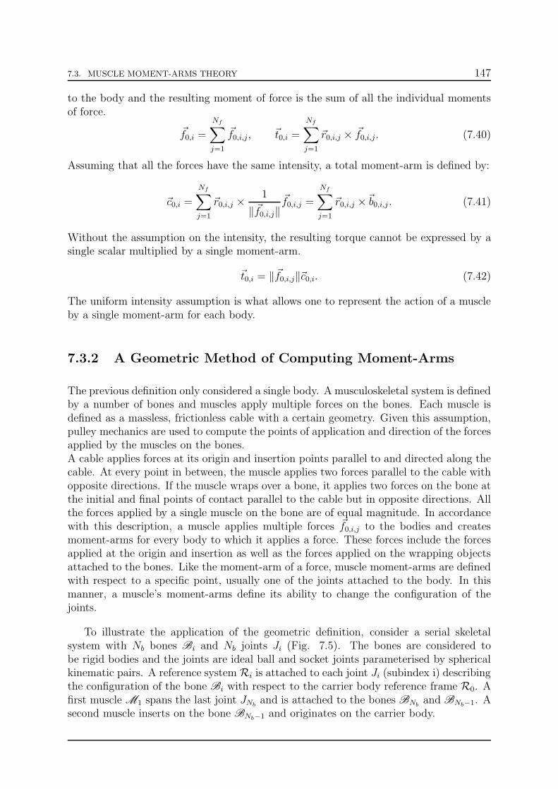
7.3. MUSCLE MOMENT-ARMS THEORY 147
to the body and the resulting moment of force is the sum of all the individual momentsof force.
~f0,i =
Nf∑
j=1
~f0,i,j, ~t0,i =
Nf∑
j=1
~r0,i,j × ~f0,i,j. (7.40)
Assuming that all the forces have the same intensity, a total moment-arm is defined by:
~c0,i =
Nf∑
j=1
~r0,i,j ×1
‖~f0,i,j‖~f0,i,j =
Nf∑
j=1
~r0,i,j ×~b0,i,j . (7.41)
Without the assumption on the intensity, the resulting torque cannot be expressed by asingle scalar multiplied by a single moment-arm.
~t0,i = ‖~f0,i,j‖~c0,i. (7.42)
The uniform intensity assumption is what allows one to represent the action of a muscleby a single moment-arm for each body.
7.3.2 A Geometric Method of Computing Moment-Arms
The previous definition only considered a single body. A musculoskeletal system is definedby a number of bones and muscles apply multiple forces on the bones. Each muscle isdefined as a massless, frictionless cable with a certain geometry. Given this assumption,pulley mechanics are used to compute the points of application and direction of the forcesapplied by the muscles on the bones.A cable applies forces at its origin and insertion points parallel to and directed along thecable. At every point in between, the muscle applies two forces parallel to the cable withopposite directions. If the muscle wraps over a bone, it applies two forces on the bone atthe initial and final points of contact parallel to the cable but in opposite directions. Allthe forces applied by a single muscle on the bone are of equal magnitude. In accordancewith this description, a muscle applies multiple forces ~f0,i,j to the bodies and createsmoment-arms for every body to which it applies a force. These forces include the forcesapplied at the origin and insertion as well as the forces applied on the wrapping objectsattached to the bones. Like the moment-arm of a force, muscle moment-arms are definedwith respect to a specific point, usually one of the joints attached to the body. In thismanner, a muscle’s moment-arms define its ability to change the configuration of thejoints.
To illustrate the application of the geometric definition, consider a serial skeletalsystem with Nb bones Bi and Nb joints Ji (Fig. 7.5). The bones are considered tobe rigid bodies and the joints are ideal ball and socket joints parameterised by sphericalkinematic pairs. A reference system Ri is attached to each joint Ji (subindex i) describingthe configuration of the bone Bi with respect to the carrier body reference frame R0. Afirst muscle M1 spans the last joint JNb
and is attached to the bones BNband BNb−1. A
second muscle inserts on the bone BNb−1 and originates on the carrier body.

148 7.3. MUSCLE MOMENT-ARMS THEORY
Carrier Body
J1
J2
J3
JNb−1
JNb
B1
B2
B3
BNb−2BNb−1 BNb
M1
M2
M2
Figure 7.5: Illustration of a skeletal system with n joints and two muscles. Muscle M1
spans a single joint. Muscle M2 spans multiple joints with m via points including originand insertion as described in section 7.3.2.
The muscle M1 spans the joint JNb, originates on the bone BNb−1 and inserts on
the bone BNb. In between it wraps over two surfaces WNb−1 and WNb
, modelling thebones. Given the location of the muscle’s origin and insertion points, the muscle createsmoment-arms at the joints JNb
and JNb−1. To define the moment-arms around the jointsJNb
and JNb−1, the two bodies are isolated (Fig. 7.6). There are three contact points withbody BNb
: PNb,1, PNb,2, PNb,3. There are three forces. The two contact points associatedto the wrapping surface and the insertion force. The total screw at the joint JNb
in thefixed frame (subindex 0) is defined by
FJNb=(
~f0,Nb,1, ~y0,Nb,1 × ~f0,Nb,1
)
JNb
+(
~f0,Nb,2, ~y0,Nb,2 × ~f0,Nb,2
)
JNb
+(
~f0,Nb,3, ~y0,Nb,3 × ~f0,Nb,3
)
JNb
,
=(
~f0,Nb,1, ~y0,Nb,1 × ~f0,n,1
)
JNb
−(
~f0,Nb,1, ~y0,Nb,2 × ~f0,Nb,1
)
JNb
+(
~f0,Nb,3, ~y0,Nb,3 × ~f0,Nb,3
)
JNb
,
=(
~f0,Nb,3, ~y0,Nb,3 × ~f0,Nb,3
)
JNb
. (7.43)
The forces applied at the points PNb,1 and PNb,2 completely cancel each other out. Themoment-arm of the muscle around the joint JNb
is thus equal to:
~c0,Nb= ~y0,Nb,3 ×
1
|f |~f0,Nb,3 = ~y0,Nb,3 ×~b0,Nb
. (7.44)
There are three contact points with body BNb−1: PNb−1,1, PNb−1,2, PNb−1,3. The jointJNb
is a ball and socket joint. It therefore transmits only forces and no moments of force.There are three forces associated to the contact points and the reaction force transmittedby the joint. This force is equal to the resulting force in the screw at the joint JNb
. Thescrew at the joint JNb−1 is defined by
FJNb−1=(
~f0,Nb−1,1, ~y0,Nb−1,1 × ~f0,Nb−1,1
)
JNb−1
+(
~f0,Nb−1,2, ~y0,Nb−1,2 × ~f0,Nb−1,2
)
JNb−1
+
(
~f0,Nb−1,3, ~y0,Nb−1,3 × ~f0,Nb−1,3
)
JNb−1
+(
~f0,Nb−1,4, ~y0,Nb−1,4 × ~f0,Nb−1,4
)
JNb−1
. (7.45)
The vector ~y0,Nb−1,4 is the vector between the joints, from JNb−1 to JNb. The force ~f0,Nb−1,4
is equal to ~f0,Nb,3 and is the inverse of ~f0,Nb−1,1. The forces at the points PNb−1,2 and PNb−1,3

7.3. MUSCLE MOMENT-ARMS THEORY 149
~f0,Nb,1
~f0,Nb,2
~f0,Nb,3
~y0,Nb,1
~y0,Nb,2 ~y0,Nb,3
~f0,Nb−1,1
~f0,Nb−1,4
~f0,Nb−1,3
~f0,Nb−1,2
~y0,Nb−1,4
~y0,Nb−1,1
~y0,Nb−1,2
~y0,Nb−1,3
JNb−1
JNb−1
JNb
JNb
JNb
WNb−1
WNb
BNb−2
BNb−1
BNb−1
BNb
BNb
M1
Moment-Arm Around JNb
Moment-Arm Around JNb−1
PNb,1
PNb,1
PNb,2
PNb,3
PNb−1,1
PNb−1,2
PNb−1,3
PNb−1,3
Figure 7.6: Isolation of the bones that the muscle M1 contacts and identification of allforces and points of application as described in section 7.3.2.
cancel each other out. The screw at joint JNb−1 reduces to the following expression
FJNb−1=−
(
~f0,n,3, ~y0,Nb−1,1 × ~f0,Nb,3
)
Jn−1+(
~f0,Nb,3, ~y0,Nb−1,4 × ~f0,Nb,3
)
JNb−1
,
=(
0, (~y0,Nb−1,4 − ~y0,Nb−1,1)× ~f0,Nb,3
)
JNb−1
. (7.46)
The resulting force at the joint JNb−1 is zero but the moment of force is not, and thereforethe moment arm is also not zero.
~c0,Nb−1 = (~y0,Nb−1,4 − ~y0,Nb−1,1)×1
|f |~f0,Nb,3 = (~y0,Nb−1,4 − ~y0,Nb−1,1)×~b0,Nb−1. (7.47)
The location of all the contact points can be computed using any one of a number ofwrapping algorithms [38, 75, 139]. Given these points, the force direction vectors ~b0,Nb
and ~b0,Nb−1 can be computed.
In the more general situation, a muscle’s moment-arm vector around a joint is com-puted by isolating the body associated to the joint and identifying all the forces which

150 7.3. MUSCLE MOMENT-ARMS THEORY
apply to it. Consider the muscle M2 from the illustration which applies forces to the bodyBi (Fig. 7.7). There are m points where forces are applied Pi,k, k = 1, 2, ..., m. The firstobservation is that the only forces which are of importance are the forces being appliedat the end points in the direction of the other bodies and the reaction force at the jointJi+1. All the other forces cancel each other. This leads to the second observation, theforce transmitted to the next body through the joint Ji along the chain in the directionof the carrier body is equal to the force being applied at the last point Pi,m. Thus, thescrew of the muscle at the joint Ji is defined by
FJi =(
~f0,i,m, ~y0,i,m × ~f0,i,m
)
Ji+(
~f0,i,1, ~y0,i,1 × ~f0,i,1
)
Ji−(
~f0,i,1, ~y0,i,m+1 × ~f0,i,1
)
Ji,
=(
~f0,i,m, ~y0,i,m × ~f0,i,m
)
Ji+(
0, (~y0,i,1 − ~y0,i,m−1)× ~f0,i,1
)
Ji. (7.48)
The muscle moment-arm around the joint Jk is defined by
~c0,i =~y0,i,m × 1
|f |~f0,i,m + (~y0,i,1 − ~y0,i,m−1)×
1
|f |~f0,i,1,
~y0,i,m ×~b0,i,m + (~y0,i,1 − ~y0,i,m−1)×~b0,i,1. (7.49)
This method of computing moment-arms is valid under the hypothesis that the bonesare rigid bodies, the muscles are ideal cables and that the joints are parameterised byspherical pairs. If the type of kinematic pairs within the musculoskeletal model aredifferent than spherical pairs, the method of computing the moment-arms would needto be adapted. Different types of kinematic pairs transfer different types of forces andmoments of force. However, the philosophy remains the same. Each body is isolated andanalysed in terms of muscle forces and joint reaction forces.
Bi
Ji
Ji+1
~y0,i,m+1
Cancellation
Cancellation
Cancellation
Only transmitted force
Pi−1,1
Pi,m
Pi,m−1
Pi,j+1
Pi,j
Pi,j−1
Pi,2
Pi,1
Pi+1,q
Figure 7.7: Illustration of force cancellations and force transmissions in a general mus-culoskeletal model as described in section 7.3.2.

7.3. MUSCLE MOMENT-ARMS THEORY 151
7.3.3 Tendon Excursion Method of Computing Moment-Arms
The second method of computing muscle moment-arms is the tendon excursion method.This method depends on the generalised coordinates used to define the model. Thismethod is derived from the principle of virtual work. Given its simplicity and relationto the experimental definition, the tendon excursion method has been widely used tocompute and validate model-based moment-arms [38, 76, 101]. However, it is a definitionthat requires caution and a certain amount of rigour. The tendon excursion method isdefined using the principle of virtual work, a concept from analytical mechanics, andmust be applied according to the same framework and hypothesis.
Consider a rigid body Bi in space that is part of a mechanism. Its configuration withrespect to a fixed frame R0 is parameterised by a Euclidean displacement function of themechanism’s generalised coordinates ~κ = (κ1, . . . , κQ)
T .
~x0,i = ~d0,i +Ri,0~xi = ~d0,i + ~x∗0,i, ~x∗0,i = Ri,0~xi. (7.50)
The velocity of the point is defined by:
~x0,i = ~d0,i + ~ω0,i × ~x∗0,i =∂~d0,i∂~κ
~κ+∂~ω0,i
∂~κ~κ× ~x∗0,i =
Q∑
k=1
∂~x0,i∂κk
κk. (7.51)
where ~ω0,i is the instantaneous rotational velocity of the body in the fixed frame. Giventhis definition of velocity, the real infinitesimal change in configuration or real infinitesimaldisplacement of the body is defined by (cf. chapter 3 for details):
d~x0,i =
Q∑
k=1
∂~x0,i∂κk
dκk =∂~d0,i∂~κ
d~κ+∂~ω0,i
∂~κd~κ× ~x∗0,i. (7.52)
A virtual displacement, is an infinitesimal displacement without an infinitesimal changein time.
δ~x0,i =
Q∑
k=1
∂~x0,i∂κk
δκk =∂~d0,i∂~κ
δ~κ+∂~ω0,i
∂~κδ~κ× ~x∗0,i. (7.53)
One of the primary differences between real and virtual displacements is that real dis-placements d~x0,i can be integrated along a path and virtual displacements δ~x0,i cannot. Ifthe mechanism’s kinematic parameterisation contains holonomic skleronomic constraintsof the form ~Φ(~κ) = (Φ1(~κ), . . .Φp(~κ))
T = ~0, both real and virtual displacements must becompatible with the constraints. The formal definition is as follows.
Definition 22 (Virtual displacement [86]). A virtual displacement δ~x0,i compatible withthe kinematic coordinates ~κ = (κ1, ..., κk, ..., κQ)
T is any displacement that can be imposedon the system satisfying the following relation:
δ~x0,i =
Q∑
k=1
∂~x0,i∂κk
δκk. (7.54)

152 7.3. MUSCLE MOMENT-ARMS THEORY
This equation is called the compatibility equation. The δqk are solutions to the equations
∑Qk=1
∂Φ1
∂κkδκk = 0,
...∑Q
k=1∂Φp
∂κkδκk = 0.
(7.55)
The virtual displacement δ~κ vector is part of the null-space of the matrix [∂Φ1
∂~κ, . . . , ∂Φp
∂~κ].
This definition states that if there are constraints, the real and virtual displacementsare in the constraint manifold’s tangent space, orthogonal to the space defined by theconstraint jacobians (cf. section 7.2.2).
There is a muscle inserting on the body Bi. This muscle applies a force ~f0,i, definedin the fixed frame at a point P (~y0,i). The virtual work created by the force, due to avirtual displacement, is defined by:
δW = ~fT0,i · δ~y0,i = ~fT0,i ·∂~d0,i∂~κ
δ~κ+ ~fT0,i ·∂~ω0,i
∂~κδ~κ× ~y0,i. (7.56)
The same force also shortens the muscle’s length by δL. The virtual work associated tothe muscle’s change in length is defined by:
δW = −f0,i · δL = −fT0,i ·∂L
∂~κδ~κ. (7.57)
The work in one-dimensional and function of the force intensity. The tendon excursionmethod is based on the hypothesis that both virtual works are equal.
δW = −fT0,i ·δL = ~fT0,i ·δ~y0,i, ⇒ −fT0,i ·∂L
∂~κδ~κ = ~fT0,i ·
∂~d0,i∂~κ
δ~κ+ ~fT0,i ·∂~ω0,i
∂~κδ~κ×~y0,i. (7.58)
The virtual change in generalised coordinates can be eliminated from the problem byrearranging the dot and cross products leading to:
−(∂L
∂~κ
)T
f0,i =
(
∂~d0,i∂~κ
)T
~f0,i +
(∂~ω0,i
∂~κ
)T (
~y0,i × ~f0,i
)
. (7.59)
The force intensity can also be removed from the expression yielding the following equiv-alence
−(∂L
∂~κ
)T
· 1 =
(
∂~d0,i∂~κ
)T
~b0,i +
(∂~ω0,i
∂~κ
)T (
~y0,i ×~b0,i)
. (7.60)
This expression states that the partial derivative of the muscle length with respect to thegeneralised coordinates is equal to the generalised muscle moment-arms. This point isfundamentally important. The tendon excursion method does not yield the moment-armsproper but the generalised moment-arms associated to the generalised coordinates. The

7.3. MUSCLE MOMENT-ARMS THEORY 153
following equality is true for models with revolute joints that all have parallel rotationaxes (one-dimensional moment-arms)
−(∂L
∂~κ
)T
=(
~y0,i ×~b0,i)
3rd coordinate. (7.61)
Thus, the coordinates used to construct the definition are not just any joint coordinates,but the generalised coordinates used to describe the musculoskeletal model. This lastpoint is key: the tendon excursion method is dependent on the choice of generalisedcoordinates and must be used accordingly. Furthermore, it is based on the principle ofvirtual displacements and therefore it must satisfy all the conditions of the definition ofvirtual displacement. The importance of this point will be illustrated in the followingsection.
7.3.4 Computing Muscle Moment-Arms
In the previous sections two definitions of moment-arms were presented. The first isgeometric and defined moment-arms using the cross-product. The second definition is thewell known tendon-excursion definition. The two definitions were shown not to be strictlyequivalent. The geometric definition yields the moment-arms proper in the inertial frame.The tendon excursion definition yields the moment-arms in the generalised coordinatespace. The definitions of moment-arms for a muscle Mj around joint Ji are given by:
Geometric definition :(
~y0,i,j ×~b0,i,j)
, ~f0,i,j = f0,i,j~b0,i,j (7.62)
Tendon excursion definition : −(∂Lj∂~κi
)T
, (7.63)
where Lj is the length of muscle Mj. The vector ~κi is the vector of generalised coordinatesparameterising joint Ji. The other coordinates are not considered. The vector ~y0,i,j is the
vector between the joint Ji and the point where muscle Mj applies a force. ~f0,i,j is theforce itself of amplitude f0,i,j. The two definitions are related by the following expression.
−(∂Lj∂~κi
)T
=
(
∂~d0,i∂~κi
)T
~b0,i +
(∂~ω0,i
∂~κi
)T (
~y0,i ×~b0,i)
. (7.64)
where ~d0,i is the displacement vector of joint i in the inertial frame. The vector ~ω0,i isthe instantaneous rotational velocity vector of the joint i in the inertial frame.
As stated in section 7.3.3, the tendon excursion method is defined from the principleof virtual work and must satisfy the conditions of the definition of virtual displacement.Given a configuration of the skeletal structure defined by the vector of generalised co-ordinates ~κ∗, the moment-arms of a muscle are computed using the tendon excursionmethod. The muscle’s length is computed for the configuration Lj(~κ
∗). The muscle’slength is then computed again after adding a small displacement δqk to each coordinate

154 7.3. MUSCLE MOMENT-ARMS THEORY
κ∗k in turn. Each generalised coordinate κk is displaced and the muscle length is computedLj(~κ
∗ + δκ∗k). The moment-arm associated to each coordinate is thus defined by:
c(κ∗k) = −Lj(~κ∗ + δκ∗k)− Lj(~κ
∗)
δκk. (7.65)
The displacement δκk is a virtual displacement and therefore must respect the conditionsof the definition of virtual displacement. These conditions are restated here.
∑Qk=1
∂Φ1
∂κkδκk = 0,
...∑Q
k=1∂Φp
∂κkδκk = 0.
(7.66)
The virtual displacements must respect the holonomic constraints. This point is fun-damental and can lead to issues during practical implementation. The musculoskeletalshoulder model presented in chapter 4 contains two holonomic constraints defining thescapulothoracic contact and a number Nw of holomomic constraints defining the wrappingsurfaces. Under the assumption that the muscle’s length is a purely kinematic quantity,the wrapping constraints for each muscle are constraints that must be respected by eachvirtual displacement. Therefore, if a fixed point of a muscle lies on the wrapping con-straint, the small displacements must be defined such that the point does not violate theconstraint. This point concerning constraints is essential and makes the tendon excursionmethod difficult to use appropriately if there are many muscles with many constraints.
Rhomboid Major Sternoclavicular Moment-Arm [m]
Scapula Fixed
Scapula Moves
Insertion Point Leaves Constraint−0.15
−0.1
−0.05
0.0
0.05
0.1
0.15
0.15
Origin
Origin
Insertion
Insertion
Wrapping
Wrapping
Surface
Surface
Initial Configuration: ~q
Initial Configuration with displacement: ~q + δ~q
X-axis Moment-Arm
Y-axis Moment-Arm
Z-axis Moment-Arm
Geometric Method
Tendon Excursion
Incompatible displacement ⇒ Constraint Violation
Figure 7.8: Illustration of how the tendon-excursion method can lead to incorrect moment-arms because the virtual displacement used to compute the moment-arm does not respectthe constraints.
To illustrate the difficulty of using the tendon excursion method appropriately, con-sider the rhomboid major muscle that originates on the thorax and inserts on the scapula.There is a wrapping constraint for this muscle that is cylinder (Fig. 7.8). The musclesegment representing the rhomboid major must pass over the surface of this cylinder. Forthis particular muscle, the insertion point of the segment lies on the surface of the cylinderin the initial configuration of the skeletal structure. If the tendon excursion method isapplied inappropriately the moment-arms differ greatly from the moment-arms computed

7.4. THE SOLUTION SET AND WRENCH-FEASIBILITY 155
using the geometric method. When the insertion point leaves the wrapping constraint,the tendon excursion method moment-arms coincide with the geometric moment-arms.However, there is a significant discontinuity of the tendon-excursion moment-arms.
By comparison, the geometric method does not rely on the principle of virtual dis-placements. Furthermore, the method does not rely on a particular choice of coordinates.It simply depends on the definition of the body frames and carrier body frames. However,the geometric method cannot easily be generalised to an algorithm. It can require a caseby case analysis of the muscles and is therefore more difficult to work with. The tendonexcursion method can be generalised more easily and is therefore favoured as a methodof computing moment-arms.
7.4 The Solution Set and Wrench-Feasibility
The previous sections showed that moment-arms are key in estimating muscle forces andreviewed the theory of moment-arms. This section re-introduces the concept of wrenchfeasibility. The concept has been extensively used in cable-driven robots [81] and hasbeen used in neuromuscular control [183]. However, it seems that it is a concept that israrely found in presentations of musculoskeletal models. The concept is related to theexistence of a solution to the muscle-force estimation problem.
In chapter 4 it is stated that models of musculoskeletal systems and models of cable-driven robots are constructed from the same hypothesis. These hypothesis include rigidbody mechanics, ideal mechanical joints and massless, frictionless, perfectly elastic mus-cles/cables. A cable-driven robot is a mechanism that is actuated by a network of ca-bles. There are two types of cable-driven robots: suspended and articulated. In sus-pended robots there is only one body connected to a frame through a network of cables[21, 80, 178]. In articulated robots there is a mechanical skeleton composed of mul-tiple bodies with joints between them and a network of cables [92, 217, 220]. In anycable-driven robot, each cable applies a system of forces to the bodies comprising themechanism and the tension in each cable is uniform. The system of forces is reduced toa single force and moment of force about one point for each body. This reduction yieldsthe body’s actuation as defined in section 7.3.1. Each cable has a motor and pulley atone end generating a tractive force within the cable by winding the cable around thepulley. The cable can only pull and its tractive strength is limited by the motor’s power.The first constraint of the cable-force coordination problem is the torque-force map. Thecables must apply the necessary actuation. The second constraint is the limitation ofthe cable’s strength. Thus, the first two constraints of the cable-force coordination prob-lem are identical to the first two constraints of the muscle-force coordination problem((7.8)-(7.9)).
~ta(~κ(tk), ~κ(tk), ~κ(tk)) = W0(~κ(tk))~fk, Torque-force constraint, (7.67)
~0 ≤ ~fk ≤ ~fmax, Min/max force bounds. (7.68)
As described in chapter 5, cost functions provide a means of differentiating the solutions

156 7.4. THE SOLUTION SET AND WRENCH-FEASIBILITY
within the feasible set. The solution set itself is defined by the constraints and the spaceof the decision variables (forces within the muscles/cables). Additional constraints fur-ther restrict the solution set defined by the first two constraints (7.8)-(7.9). Therefore,the muscle-force coordination problem defined in section 7.2.1 is mathematically almostidentical to the cable-force coordination problem of cable-driven robots. Both coordina-tion problems are defined by nonlinear programs. Their purpose being to compute therequired forces in the muscles/cables to drive the system (skeleton/mechanism) along apre-defined kinematic path. Therefore, theory regarding the force coordination problemthat has been developed for models of cable-driven robots can be applied to models ofmusculoskeletal systems such as the shoulder.
For both coordination problems, solving the NLP is straightforward [14, 24, 35]. Thereexist numerous NLP solvers. However, the question of the existence of a solution is not.In cable-driven robotics, this question is called wrench feasibility [21, 81, 146]. At the coreof the analysis is the torque-force map (7.75) governing the solutions to the NLP. At agiven instant tk, the relation between the forces in the cables and the actuation applied tothe system, defines a linear map between two vector spaces. The force intensity space F
which is a subset of RNp and the tangent space of the coordinate manifold T~κ(tk)QS ⊂ RD,
where D is the number of degrees of freedom.
Mk : F → T~κ(tk)QS,
~fk 7→ Mk(~fk) = ~ta(~κ(tk), ~κ(tk), ~κ(tk)) = W0(~κ(tk))~fk. (7.69)
For a system with Np forces, the upper and lower bounds (7.68) on the forces (withoutadditional constraints) define the map’s domain space F as a convex polytope2 in R
Np .The geometry of the domain space polytope is defined by the values of ~fmax. The imageof a convex polytope under linear transformation is a convex polytope [87]. The imagespace Mk(F ) is therefore also a convex polytope in T~κ(tk)QS. The geometry of the imagespace polytope is defined by Mk(~fmax).
Definition 23 (Torque Set Wreq(~κ)). The torque set Wreq(~κ) is the set of actuation vectors
that the cables must be able to produce for a given kinematic configuration (~κ, ~κ, ~κ).
Wreq(~κ) = ~ta ∈ T~κQS ⊂ RD. (7.70)
Definition 24 (Wrench-Feasible Workspace and Torque-Feasible Space). The wrench-feasible workspace is the set of kinematic configurations (~κ, ~κ, ~κ) such that for any actu-
ation vector ~ta ∈ Wreq(~κ), there is a vector of cable forces ~f ∈ F satisfying
~ta = W0(~κ)~f. (7.71)
The actuation vectors belong to the torque-feasible space.
Given this definition of wrench-feasible workspace, a system is said to be wrench-feasible if the following condition holds [21, 57]:
Wreq(~κ) ⊂ Mk(F ), ∀(~κ, ~κ, ~κ) ∈ TQS. (7.72)
2A polytope is a geometric object with flat sides. Examples include polygons in 2-dimensions andpolyhedrons in 3-dimensions.

7.4. THE SOLUTION SET AND WRENCH-FEASIBILITY 157
The torque set must be a subset of the image set of the force intensity space. Thiscondition guarantees the existence of a solution to force coordination problem.
In cable-driven robotics, wrench-feasibility is a design criterion. In musculoskeletalsystems, although the real system is already wrench-feasible, the model must be well de-fined such that wrench-feasibility naturally occurs. Design of the cable/muscle structureis the design of the moment-arms matrix. Thus, again the moment-arms matrix is thekey element in muscle-force estimation.
M1
M2
M3
J1
J2
Eϑ1ϑ2
B1: M1, I1 B2: M2, I2
Figure 7.9: A two-dimensional toy musculoskeletal model used to illustrate the discussionof section 7.4.
To illustrate wrench feasibility, consider a musculoskeletal model with two bones B1
and B2 (Fig. 7.9). The bones are connected through a revolute joint J2 and the first boneis connected to a carrier body through a second revolute joint J1. There are three musclesactuating the skeletal structure. The first muscle M1 spans the revolute joint J1. Thesecond muscle M1 spans both joints. There is a cylinder aligned with the second joint’srotation axis to constrain the muscle paths. The third muscle M3 spans the revolutejoint J2. The configuration of the skeletal structure is defined by the configurations ofthe revolute joints which are parameterised by the angles ~κ = (ϑ1, ϑ2)
T . The coordinatemanifold QS is S1 × S1.
f1
f2
f3ta,2
ta,1
~f =
f1f2f3
F = [0, 125]× [0, 75]× [0, 200] ⊂ R3
~ta(tk) = Mk(~f) =
(ta,1ta,2
)
Mk
The necessary actuation vectormust remain inside this area.
Mk(F ) ⊂ T~κ(tk)QS ⊂ R2
Figure 7.10: Range and image spaces of the torque-force map for the musculoskeletalmodel presented in section 7.4 and illustrated in figure 7.9.
The dynamics of the system are the dynamics of a double pendulum with distributed

158 7.4. THE SOLUTION SET AND WRENCH-FEASIBILITY
mass [209]. There are two equations of motion and the actuation vector is defined by:
~ta =
(ta,1ta,2
)
= M(ϑ1, ϑ2)~κ−~h(~κ, ~κ) = W0(~κ)~f. (7.73)
There are three cable-force intensities. The torque-force map is defined by:
Mk : F ⊂ R3 → T~κ(tk)QS ⊂ R
2,
~fk 7→ Mk(~fk) = ~ta(tk) = W0(~κ(tk))~fk. (7.74)
The first muscle always creates a moment-arm around the joint J1. The second andthird muscles define moment-arms around both joints. The moment-arm matrix has thefollowing structure:
~ta =
(ta,1ta,2
)
= M (~tg) = W0(~κ)~f =
(w1,1(ϑ1) w1,2(ϑ1, ϑ2) w1,3(ϑ1, ϑ2)
0 w2,2(ϑ2) w2,3(ϑ2)
)
f1f2f3
. (7.75)
The muscles are attributed different maximum forces: f1,max = 125[N ], f1,max = 75[N ],f3,max = 200[N ]. All the physical constants are set to 1, including the lengths of thependulum’s links.As the configuration of the mechanism changes, the image space polytopeMk(F ) changesshape (Fig. 7.11). The mechanism is wrench feasible as long as the necessary actuation~ta remains inside the image space polytope, and this for any configuration ~κ = (ϑ1, ϑ2)
T .
−60 −40 −20 0
0
10
20
30
40
50
60
−20 −10 0 10 20
−10
−5
0
5
10
15
20
25
−10 0 10 20
−15
−10
−5
0
5
10
15
20
−60 −40 −20 0
0
10
20
30
40
50
60
Joint 1 Actuation: ta,1Joint 1 Actuation: ta,1Joint 1 Actuation: ta,1
Joint2Actuation:t a
,2
ϑ1 = 0, ϑ2 = 0 ϑ1 = 45, ϑ2 = −45
ϑ1 = −45, ϑ2 = 45
Figure 7.11: Image space of the torque-force map in three different configurations for themusculoskeletal model presented in section 7.4 and illustrated in figure 7.9.
For a path ~κ(t) in the configuration space, the set Mt(F ) defines the time-dependentbehaviour of the image space polytope. The image space depends only on the set ofconfigurations ~κ(t) that the path passes through. The system remains wrench-feasible aslong as the necessary actuation to perform the motion remains within the image spacepolytope for the entire motion. The wrench-feasibility condition will limit how fast themotion can be performed. At slower speeds, the required actuation is smaller and morelikely to be inside Mt(F ), whereas at higher speed, the actuation vector increases andcan leave Mt(F ).

7.5. CONCLUSIONS 159
The concept of wrench-feasibility allows one to design the musculature as a collective[183]. This result complements the result regarding the modelling of large muscles [197].The previous result states how best to model each muscle individually. Wrench-feasibilityuses that result as a basis for improving the muscle model as a collective. Therefore, bothresults combined provide a tool for developing improved geometric muscle models. Theuse of wrench feasibility will be illustrated in the following chapter.
Joint 1 Actuation: ta,1
Joint2Actuation:t a
,2
Time t [s]00.2 0.4 0.6 0.8
1
-20
-10
0
10
20
30~ta, t = 0 [s]
~ta, t = 0.2 [s]~ta, t = 0.4 [s]
~ta, t = 0.6 [s] ~ta, t = 0.8 [s]
~ta, t = 1 [s]
-50
0
50
Figure 7.12: Illustration of the time-dependent behaviour of the image space polytope forthe musculoskeletal model presented in section 7.4 and illustrated in figure 7.9.
7.5 Conclusions
The goal of this chapter was to present the muscle-force coordination strategy used to es-timate the forces in the musculoskeletal shoulder model presented in chapter 4. Based onthis presentation, moment-arms were shown to be the key element governing muscle-forceestimation. Therefore, this chapter reviewed the theory of moment-arms by discussingthe fundamental geometric concepts behind moment-arms and presenting the tendon-excursion method of computing moment-arms. This chapter showed that the tendonexcursion method does not yield the muscle moment-arms in the geometric sense. Thetendon excursion method and geometric definition of moment-arms are related througha projection matrix from analytical mechanics. Finally, this chapter re-introduced a rel-atively new concept with respect to musculoskeletal modelling called wrench-feasibility.The concept complements the already existing results concerning muscle-force estimationby providing information regarding the possible movements, the system can perform. Thelimitations on the muscle forces defines limitations on the possible movements that themodel can realise. These limitations can be pre-analysed without solving the muscle-forceestimation problem by computing the torque-feasible set. The troque-feasible set can beused to improve the model of the musculature.

160 7.5. CONCLUSIONS

Chapter 8
Estimating Joint Force in the
Human Shoulder
8.1 Introduction
Osteoarthritis or degenerative arthritis is the most common form of arthritis and is justone of the many dysfunctions affecting the human musculoskeletal system. In the shoul-der, it causes premature degradation of the glenohumeral or shoulder joint and is quitepainful. The degradation is the result of frequent inappropriate mechanical loading ofthe articular cartilage [27] (cf. chapter 2 for anatomical references). To help understandosteoarthritis of the shoulder, it necessary to have an estimate of how the articular carti-lage is being loaded in healthy and dysfunctional shoulders. This information is criticalin the development of treatments of osteoarthritis.In general, the stress occurring in the articular cartilage cannot be measured. In recentyears a prothesis of the humeral bone has been developed containing a load sensor [201].The measurements obtained from such a device are a good indicator of the stress but arenot a completely accurate representation of the loading given that part of the shoulderhas been replaced with a prosthesis. We must therefore continue to rely on musculoskele-tal models to estimate the stress occurring in the articular cartilage of joints affected byosteoarthritis.
There are a number of musculoskeletal models of the shoulder that have been de-veloped for the purpose of studying the forces in the glenohumeral joint. There is theDelft shoulder and elbow model (DSEM). Constructed in 1994 [194], the model has beenrecently validated as a model for measuring the force in the glenohumeral joint [155]. Thevalidation process was done using data collected by the shoulder prosthesis mentionedpreviously [156]. There is the AnyBody R© shoulder model. Developed for multiple pur-poses [49], the model has been used to specifically estimate the force in the glenohumeraljoint [158]. There is the model developed at the ETH Zurich Switzelrand. Developed foranalysing the stability of the glenohumeral articulation [71], the model uses an algorithmdesigned specifically for computing the force in the glenohumeral joint [70]. Finally there
161

162 8.2. METHODS
is the Newcastle model. The model was initially developed for analysing the forces in theglenohumeral joint during activities of daily living [37] and has since been used to studythe effects of surgery on the joint force [120].Although these models are high fidelity models and are successful in estimating gleno-humeral joint forces, the consensus of the International Shoulder Group (ISG)1 is thatthere still remains a considerably large gap between models and reality [47, 48]. Giventhat there is no perfect match between simulations and experiments [182], future researchshould focus on clinical validation. A musculoskeletal model must be validated beforeit can be used to make conclusions regarding musculoskeletal systems. Validation con-stitutes the most challenging task of musculoskeletal modelling once a model has beenconstructed [135].
The goal of this chapter is to present the implementation of the musculoskeletal shoul-der model discussed in chapter 4. The model is being designed specifically for the purposeof estimating the force in the glenohumeral joint. The model is to be used in parallel witha finite element model of the glenohumeral joint [59]. The chapter begins by reviewingthe model’s characteristics and the methods from chapters 6 and 7 to solve its kinematicredundancy and overactuation. The chapter then introduces the computational proce-dure used to compute the models outputs that are muscle forces and the joint reactionforce in the glenohumeral joint. The model is used to estimate the forces during fastand slow abduction in the scapular plane. The results are presented in terms of scapu-lar kinematics, muscle moment-arms, muscle forces, joint reaction forces (intensity andorientation). The results are discussed and compared to results from the literature. Thechapter concludes with a brief discussion regarding the models current most importantweakness and suggestions on how to improve it.
8.2 Methods
8.2.1 A Musculoskeletal Model of the Human Shoulder
This section presents a brief review of the musculoskeletal shoulder model from chapter4. The model is a right shoulder of an adult male. It includes the thorax, clavicle,scapula and humerus. The thorax is the carrier body to which the inertial referenceframe is attached R0. A reference frame Ri is also defined for the clavicle, scapula andhumerus (Fig. 8.1). The reference frames are defined according the guide lines set by theInternational Society of Biomechanics (ISB) [214] (cf. chapter 4). Subindexes are usedto identify each frame: thorax: 0, clavicle: 1, scapula: 2, humerus: 3.
The three synovial articulations (sternoclavicular SC, acromioclavicular AC andglenohumeral GH) are modelled as ideal ball and socket joints and parameterised usingspherical kinematic pairs. The configurations of the sternoclavicular and acromioclavic-
1The ISG is a collaboration of biomechanics research groups who’s main focus is the shoulder. It isalso one of the many technical groups of the International Society of Biomechanics (ISB).

8.2. METHODS 163
ular spherical pairs are described using two sets of Bryan angles: ~ΥT1 = (ψ1, ϑ1, ϕ1)
T
and ~ΥT2 = (ψ2, ϑ2, ϕ2)
T . The rotation sequence is XYZ. The configuration of the gleno-
humeral spherical pair is described using Euler angles: ~ΥT3 = (ψ3, ϑ3, ϕ3)
T . The rotationsequence is ZYZ. The shoulder’s configuration is parameterised by a vector of nine jointangles.
~q =(~ΥT
1~ΥT
2~ΥT
3
)T=(ψ1 ϑ1 ϕ1 ψ2 ϑ2 ϕ2 ψ3 ϑ3 ϕ3
)T. (8.1)
Three Euclidean displacements are defined that map vectors in a local frame to vectorsin the inertial frame. The displacements are parameterised by the vector of coordinates~q using the standard charts on SO(3) to build the rotation matrices (cf. chapters 4 and6 for details on constructing the rotation sequences).
P0,i : ~p0,i = ~d0,i +Ri,0(ψi, ϑi, ϕi)~pi. (8.2)
The vector ~d0,i is the translation vector from the centre of the inertial frame to the centreof the local frame, defined in the inertial frame (cf. chapter 3 for notations regardingEuclidean displacements). The matrix Ri,0 is the rotation matrix from the local frameRi to the inertial frame R0.
R0
R1
R1
R2
R2
R3
R3
ψ1
ϑ1
ϕ1
ψ2
ϑ2
ϕ2
ψ3
ϑ3
ϕ3
Joint Coordinate Definitions:
IJ
IJ
PX
T8
T8
C7
C7
SCAC
AC
AA AA
TS
AIGH
GH
HU
EL
EM
Figure 8.1: Illustration of the bony landmarks, reference frame and the locations of thebone centres of gravity. Image created using ZygoteBodyTM zygotebody.com.
The scapulothoracic contact is modelled by constraining two points on the scapula’smedial border to remain on the surface of two ellipsoids. The ellipsoids have identical

164 8.2. METHODS
centres but different dimensions and are aligned with the inertial frame. The ellipsoidsmodel the surface of the ribcage with an additional layer of muscle. The points definingthe constraints are the trigonum spinae (TS) and the angulus inferior (AI). They are theend-points of the scapula’s medial border. The ellipsoids are defined in the thorax frameyielding the following two holonomic skleronomic constraints.
ΦTS(~Υ1, ~Υ2) = (~u0,2 − ~e0)TETS (~u0,2 − ~e0)− 1 = 0, TS0,2 : ~u0,2 = ~d0,2 +R2,0~u2, (8.3)
ΦAI(~Υ1, ~Υ2) = (~v0,2 − ~e0)T EAI (~v0,2 − ~e0)− 1 = 0, AI0,2 : ~v0,2 = ~d0,2 +R2,0~v2. (8.4)
where ~e0 is the point vector of the centre of the ellipsoid E common to both constraints,in the inertial frame. The matrices ETS and EAI are the quadric matrices of each ellipsoid(cf. appendix A).
The forward kinematic map defines the map from the joint coordinates to the spatialconfiguration of the end-effector. The end-effector is defined as the centre of the humer-oulnar joint (HU). Its spatial configuration is defined as the position of the humeroulnarjoint centre HU and the orientation of the humerus.
ΞS : QS → WS,
~q 7→ ΞS(~q) = Ce =(
~ǫT0,3,~ΥT
3
)T
, HU0,3 : ~ǫ0,3 = ~d0,3 +R3,0~ǫ3, (8.5)
s.t. ΦTS(~Υ1, ~Υ2) = (~u0,2 − ~e0)TETS (~u0,2 − ~e0)− 1 = 0, (8.6)
ΦAI(~Υ1, ~Υ2) = (~v0,2 − ~e0)T EAI (~v0,2 − ~e0)− 1 = 0. (8.7)
The kinematic model has seven degrees of freedom. The map is parameterised by thenine kinematic coordinates (8.1) and subject to the two scapulothoracic constraints.
Each body is given a mass Mi and an inertia Ii defined with respect to the centreof gravity [28]. The clavicle’s centre of gravity is located at the mid-point along theaxis between the SC and AC joints. The scapula’s centre of gravity is located one thirdof the way along the axis between the AC and AI points, starting from the AC point.The humerus centre of gravity also defining the arm’s centre of gravity, is located at thepoint HU. The arm is considered to always be outstretched. The equations of motion areobtained using the Euler-Lagrange equation. The generalised coordinates are defined asthe kinematic coordinates: ~κ = ~q. The total lagrangian is the sum of the bone lagrangiansaugmented by the constraints (cf. chapter 3 and 4). The dynamic model is defined by:
∂2L∂~κ2
~κ+∂2L∂~κ∂~κ
~κ− ∂L∂~κ
= W0(~κ) ~f, (8.8)
s.t. ΦTS(~κ) = (~u0,2 − ~e0)TETS (~u0,2 − ~e0)− 1 = 0, (8.9)
ΦAI(~κ) = (~v0,2 − ~e0)T EAI (~v0,2 − ~e0)− 1 = 0, (8.10)
where L is the sum of the bone lagrangians. As presented in chapter 7, the constraintforces (scapulothoracic contact forces) and muscle forces are grouped into a single vector
~f . The matrix W0 is the generalised moment-arm matrix defined with respect to theinertial frame. The muscles can only pull and the scapulothoracic contact forces are

8.2. METHODS 165
only compressive forces. They cannot pull the scapula onto the surface of the ellipsoid.Furthermore, the muscles have a maximum isometric strength [76] and the contact forcesare limited using the observations from [88, 195]
~0 ≤ ~f ≤ ~fmax. (8.11)
The geometric muscle model was constructed using the framework set in [76]. The 16anatomical muscles are divided into 28 segments and wrapping constraints are definedfor each segment using the algorithms from [75]. Thus, the wrapping constraints andtopology of the geometric muscle model are identical to the model defined in [76] but thenumerical values are different. Furthermore, in chapter 4 it is stated that each musclesegment can be parameterised by one or more cable(s). The musculature in the presentmodel is represented by Np ≥ 28 cables.
8.2.2 Kinematic Coordination
The forward kinematic map (8.5)-(8.7) is parameterised by nine angular coordinatessubject to two holonomic skleronomic constraints. This map is the structure for thedynamic model. In chapter 6, a method of planning the model’s kinematics is presented.The method proposes an alternate set of coordinates ~ζ that can be used to construct atime-dependent parameterisation of the joint angles ~q. The coordinates are called minimalcoordinates because their number is equal to the number of degrees of freedom. They areindependent and make kinematic computations more straightforward. Optimisation canbe used but is no longer required.
The minimal coordinates are defined using the lower scapulothoracic kinematic map.In chapter 6, the scapula is shown to be equivalent to a rigid body constrained to glideover three surfaces through punctual contacts AC, TS and AI. The surfaces are a spherecentred at SC, an ellipsoid centred at E and a second ellipsoid centred at E of differentdimensions. According to this description, the minimal coordinates are defined as follows.The first coordinate ζ1 parameterises the clavicle’s axial rotation and is equivalent tothe angular coordinate ψ1. The last three coordinates ζ5, ζ6 and ζ7 parameterise theglenohumeral motion and are equivalent the glenohumeral joint Euler angles (ψ3, ϑ3, ϕ3).The three remaining coordinates ζ2, ζ3 and ζ4 parameterise the configuration of thescapula. The point AI is located by the two spherical coordinates (αAI, βAI) ≡ (ζ2, ζ3)parameterising the ellipsoid on which it glides.
AI =
xe + aAI cos(αAI) sin(βAI),ye + bAI sin(αAI) sin(βAI),ze + cAI cos(βAI).
~e0 =
xeyeze
(8.12)
where aAI, bAI, cAI are the ellipsoid axial dimensions. The point TS is constrained onthe ellipsoid ΦTS (8.10) and is at a fixed distance from AI. The point is located by theintersection of a sphere centred at AI and the ellipsoid ΦTS. The intersection betweentwo such quadrics is well defined and is homeomorphic to a circle. The coordinate ζ4parameterises the intersection. Once the locations of the points AI and TS are known,

166 8.2. METHODS
the point AC is known by trilateration [125]. It lies on the intersection of three spheres.The coordinates ζ2, ζ3 and ζ4 parameterise thoraco-scapular motion and are equivalent tothe five joint angles (ϑ1, ϕ1, ψ2, ϑ2, ϕ2). The relation between the joint angle coordinates~q and the minimal coordinates is summarised by:
ζ1 ≡ ψ1,ζ2 ζ3 ζ4 ≡ ϑ1 ϕ1 ψ2 ϑ2 ϕ2,ζ5 ζ6 ζ7 ≡ ψ3 ϑ3 ϕ3.
Clavicle axial rotation,
Thoraco-Scapular motion,
Glenohumeral motion rotation.
Given the set of minimal coordinate, kinematic coordination of the shoulder model isachieved by first planning the motion in terms of the minimal coordinates ~ζ. Once amotion is constructed in terms of ~ζ(t), it is mapped to a motion in terms of ~q(t). Forcoordinates ζ1, ζ5, ζ6 and ζ7 the mapping is the identity map. For the coordinates ζ2, ζ3and ζ4, the five angular coordinates (ϑ1, ϕ1, ψ2, ϑ2, ϕ2) are obtained by constructing therotation matrices R1,0 and R2,0, using the geometric location of the points AC, AA, TSand AI with respect to the inertial frame. Once the rotations are known the angles areextracted using the inverse trigonometric functions. The joint angles ~q(t) are equivalentto the generalised coordinates ~κ(t).
The parameterisation is defined over the interval t ∈ [0, 1]. The first and secondderivatives are obtained numerically. The dynamic behaviour is further defined by settingthe time horizon T . As T increases, the behaviour becomes more quasi-static. Oppositely,as T decreases, the behaviour becomes more dynamic.
~κ(tk) =~κ(tk+1)− ~κ(tk)
T (tk+1 − tk), ~κ(tk) =
~κ(tk+2)− 2~κ(tk+1) + ~κ(tk)
T 2(tk+2 − tk+1)(tk+1 − tk), ∀tk ∈ [0, 1]. (8.13)
SC
SC
AC
AC
GHGH
TS
AI
AAAA
E
ψ3
θ3
φ3
ψ1
αAI
βAI
ξTS
Sphere-ellipsoidintersection locus
Figure 8.2: Illustration of the minimal coordinates used to coordinate the shoulder asdefined in section 8.2.2. Image created using ZygoteBodyTM zygotebody.com.
The model has thus far been used for humeral abduction in the scapular plane. Thetime-dependent parameterisation of the minimal coordinates was defined using a dataset

8.2. METHODS 167
from the literature [58]2. This particular dataset was chosen because it was specificallyconstructed to obtained measured shoulder kinematics. The data contains the location ofall the bony landmarks necessary to implement the kinematic model. The bony landmarkswere obtained by transformation of their corresponding measured skin markers [56]. Thedataset also contains a single ellipsoid that was used to construct the two ellipsoidsnecessary for the model described in this thesis. The single ellipsoid was rotated suchthat its axes coincide with the inertial frame axes. The ellipsoid was then uniformlydilated twice to produce two ellipsoids with identical centres. The dilation coefficientwas obtained such that TS and AI lie on their respective ellipsoids. Finally, the dataset contains measured values of the three scapular angles ψ2, ϑ2 and ϕ2 during humeralabduction in the scapular plane for six subjects. The measurements were taken at 0,45, 90, 120, 140 and 160 humeral abduction. The minimal coordinates were plannedto match these values as closely as possible.
Table 8.1: Joint angle terminology. The joint angles are defined in chapter 4.ψ1 ≡ ζ1 Axial Rotation ψ2 Anterior/Posterior Tilt ψ3 ≡ ζ5 Axial Rotation
ϑ1 Depression/Elevation ϑ2 Depression/Elevation ϑ3 ≡ ζ6 Elevation
ϕ1 Protraction/Retraction ϕ2 Protraction/Retraction ϕ3 ≡ ζ7 Elevation Plane
Using the dataset, each coordinate ζi(t) was planned according to the description ofhumeral abduction presented in chapter 3. Between 0 and 30 abduction, the scapularcoordinates ζ2, ζ3 and ζ4 were held constant at their initial values. Between 30 and160 abduction, the scapular coordinates were planned using a linear function of time.The clavicle’s axial rotation coordinate ζ1 was held constant during the first 30 humeralabduction and then rotated posteriorly by 40 using a linear function of time. Theglenohumeral coordinates ζ5 and ζ7 were held constant at 0 and 30 to obtain abductionin the scapular plane with no internal rotation. The third glenohumeral coordinate ζ6was planed using a linear function of time.
ζ1(t) =
0, t ∈ [0, 30/160]0 + 40t, t ∈ [30/160, 1]
(8.14)
ζ2(t) =
ζ2(0), t ∈ [0, 30/160]ζ2(0) + (ζ2(1) − ζ2(0))t, t ∈ [30/160, 1]
(8.15)
ζ3(t) =
ζ3(0), t ∈ [0, 30/160]ζ4(0) + (ζ3(1) − ζ3(0))t, t ∈ [30/160, 1]
(8.16)
ζ4(t) =
ζ4(0), t ∈ [0, 30/160]ζ3(0) + (ζ4(1) − ζ4(0))t, t ∈ [30/160, 1]
(8.17)
ζ5(t)= 0, t ∈ [0, 1] (8.18)
ζ6(t)= 0 + 160t, t ∈ [0, 1] (8.19)
ζ7(t)= 30, t ∈ [0, 1] (8.20)
The initial values ζ2(0), ζ3(0) and ζ4(0) are obtained from the location of the bony land-marks at 0 abduction. The values ζ2(1), ζ3(1) and ζ4(1) are selected appropriately to
2The dataset was provided courtesy of the Laboratoire de Biomecanique et Mecanique des Chocs,Universite de Lyon

168 8.2. METHODS
obtain a configuration of the scapula which is consistent with the measured configurationsat 160 abduction. The values were set by hand, but an optimisation method could alsobe used.
8.2.3 Muscle-Force Coordination
In chapter 7, the proposed muscle-force coordination strategy is to impose a desiredmotion and use the model’s inverse dynamics (8.8)-(8.10) to obtain the required actuationtorque for each joint. The desired kinematics reduce to a single vector ~ta(~κ, ~κ, ~κ) calledthe actuation vector. Given this torque, the muscle forces are computed by solvinga non-linear program. As stated in chapter 7, the central equation of of muscle-forcecoordination is the relation between the kinematics and the muscle forces.
∂2L∂~κ2
~κ+∂2L∂~κ∂~κ
~κ− ∂L∂~κ
= ~ta(~κ, ~κ, ~κ) = W0(~κ) ~f. (8.21)
This relation defines the inverse dynamic model used to coordinate the muscle forces.Using the same terminology as chapter 5, the primary task is the kinematics. By imposingthis task, a set of solutions has already been differentiated from the complete set ofsolutions for any kinematics. The muscle forces must generate the desired kinematics.The next phase is to use a secondary task to differentiate a single solution from withinthe subset.Given the desired kinematics (~κ(t), ~κ(t), ~κ(t)), a single solution to (8.21) is differentiatedfrom the subset using a static optimisation problem for a finite number of instances tk.The set of solutions is further differentiated by imposing the bounds on the muscle forces(8.11) and the glenohumeral stability constraint (cf. chapter 7). The secondary task isthe cost function of the optimisation problem. It has been shown that minimising themean square muscle stress yields solutions that agree with measured muscle forces [195].This cost function has been selected, although others are possible [167, 172].Muscle stress is defined as the muscle’s force divided by the physiological cross-sectionalarea (PCSA). The optimisation problem uses the primary task as a constraint. Thisconstraint is called the torque-force constraint.
min~fk
Γ( ~fk) =1
2
p∑
j=1
( ~f2j )k
PCSA2j
=1
2~fTk P
~fk, (P)i,j =δi,j
PCSA2j
. (8.22)
s.t. ~ta(~κ(tk), ~κ(tk), ~κ(tk)) = W0(~κ(tk))~fk, Torque-force constraint, (8.23)
~0 ≤ ~f ≤ ~fmax, Min/max force bounds, (8.24)
~g(~κ(tk), ~κ(tk), ~κ(tk), ~fk) ≤ ~0, GH stability constraint. (8.25)
A solution to this problem is found using null-space optimisation. The muscle-force vectoris parameterised directly in terms of the primary task or torque-force constraint. Thesolution is defined by:
~fk = ~f ∗k+Nk~vk, ~f ∗
k = W+
0 (~κ(tk)) ~ta(~κ(tk), ~κ(tk), ~κ(tk)) W0(~κ(tk))Nk = 0. (8.26)

8.2. METHODS 169
where ~f ∗k is an initial solution obtained by taking the Moore-Penrose pseudo-inverse of the
generalised moment-arms matrix W0(~κ(tk)). This particular pseudo-inverse minimisesthe mean-square muscle stress if it is weighted by the PCSAs [203]. The initial solutiondoes not however satisfy the other two constraints. The vector ~vk parameterises the null-space Nk of the generalised moment-arms matrix. This parameterisation is inserted intothe cost function (8.22) yielding a quadratic optimisation problem (c.f. chapter 7 fordetails).
min~vk
Γ(~vk) =1
2~vTk N
T
k PNk~vk + ( ~f ∗k )T PNk~vk, (8.27)
s.t. Ak~vk −~bk ≤ ~0, (8.28)
The null-space of the moment-arms matrix is used to change the initial solution withoutviolating the primary task while realising the secondary task and satisfying the additionconstraints.
Once the solution to the muscle-force coordination problem is found, the glenohumeraljoint reaction force is computed. The constraint forces are removed from the solutionyielding ~f , containing just the muscle forces. As stated previously in section 8.2.2, the
scapulothoracic contact forces are included in the vector ~f and must be removed beforecompute the joint reaction force. The glenohumeral reaction force ~fr is computed fromthe expression of the arm’s translational dynamics (Newton’s second law of motion).
M3~x0,3 =M3~g0 +D0~f + ~fr, (8.29)
whereM3 is the arm’s mass. The vector ~x0,3 is the arms translational acceleration definedin the inertial frame. The vector ~g0 is the earth’s gravitational vector field defined in theinertial frame. The matrix D0 is the force direction matrix defined in the inertial frame.
8.2.4 Implementation and Model Output
The musculoskeletal model of the human shoulder presented in chapter 4 and brieflyreviewed in section 8.2.1 was implemented into the Mathworks computing environment:MATLAB (Version 2014a for Mac) (Fig. 8.3). The necessary physical data (bony land-marks, muscle insertions and origins, etc.) to construct the model was collected fromMRI scans of an adult male [60]. All the data required to reconstruct and implement themodel can be found in appendix B.
The model is being designed to estimate the force in the glenohumeral joint. Asstated previously the general methodology is to define a kinematic motion. The inversedynamics model is used to compute the associated actuation vector. The muscle-forcesthat generate the actuation vector are found through a static optimisation program.Once the muscle-forces are found, the joint reaction force is obtained using the arm’stranslational dynamics. The computational procedure for obtaining the glenohumeraljoint reaction force for a given movement is defined as follows:

170 8.2. METHODS
Glenohumeral Joint-Force Estimation Computational Procedure:
1. A motion of the skeletal system is planned using the minimal coordinates ~ζ(t).The motion is planned over the time horizon t ∈ [0, 1] for N evenly distributeddiscrete instances.
2. The same motion is computed in terms of the generalised kinematics ~κ(t), ~κ(t)and ~κ(t). The dynamic behaviour is defined by setting the time horizon T(8.13).
3. The necessary actuation vector ~ta(~κ(t), ~κ(t), ~κ(t)) is computed using the inversedynamic model (8.21). The lagrangians are computed using the method pre-sented in chapter 3.
4. For each time step tk ∈ t0, t1, . . . , tN = T the muscle-force coordination prob-lem is solved using the quadratic optimisation problem (8.27), (8.28). Themoment-arms matrix is computed using the geometric method from chapter 7.The problem is numerically solved using MATLAB’s quadprog function. Theupper bounds on the muscle forces are taken from [76].
5. The scapulothoracic contact forces are removed from the solution to yield themuscle forces ~f(tk). The glenohumeral joint reaction force ~fr(t) is computedusing the arms translational dynamics (8.29). These dynamics are computedusing the method presented in chapter 3.
The model’s performance is evaluated with respect to four points that cover theimportant aspects of muscle and joint-force estimation. The results will be presentedin terms of these points.
• Scapular kinematics: The most challenging point of kinematic shoulder mod-elling is the description of scapular kinematics due to the scapulothoracic con-straints. The model-predicted scapular kinematics are compared to the measuredscapular kinematics from [58].
• Muscle moment-arms: The muscle-force coordination strategy is centred aroundthe moment-arms matrix. The moment-arms are compared to measured moment-arms from cadaveric studies [2, 102, 130, 161]. In cadaveric studies, the rotator cuffmuscle moment-arms are measured for humeral abduction in the scapular plane.the scapula remains fixed and the humerus is abducted up to 90 in the scapularplane. The moment-arm of each muscle in the rotator cuff is measured in termsof its component around the y-axis normal to the scapular plane. The model’smoment-arms were also compared to the moment-arms from the Visible HumanProject (VHP) kinematic model [76]. This comparison is well founded, given thatthe two models share the same muscle topology. The present model’s geometricmuscle model was constructed using the same framework.

8.2. METHODS 171
• Muscle-forces: The model is designed to estimate muscle forces. The muscleforces are presented for quasi-static (T = 20 [s]) and dynamic (T = 2 [s]) abductionin the scapular plane. The computation was done for 100 points evenly distributedbetween 0 and 140 abduction. The computation was stopped at 140 becausethe model’s validity is questionable for high abduction angles. The estimation wasperformed using 28 muscle segments (one segment per muscle).
• Joint reaction force intensity and orientation: Is the primary objective ofthe model. The joint reaction force intensity for quasi-static abduction is comparedto results reported in [10, 71, 155]. The joint force orientation with respect to theglenoid is compared to results reported in [59, 195].
Figure 8.3: Illustration of the musculoskeletal shoulder model implemented into the Math-works computing environment: MATLAB (Version 2014a for Mac).

172 8.3. RESULTS
8.3 Results
8.3.1 Scapular Kinematics
For humeral abduction in the scapular plane, the model predicted scapular kinematicsshow protraction, depression and posterior tilt (Fig. 8.4). The scapula protracts forwardsaround the ribcage and depresses. The movement of the lowest point on the scapula (an-gelus inferior AI) creates posterior tilt. The elevation/depression angle shows the largestvariation between initial and final values.For all three angles, the minimal coordinate-constructed scapular kinematics remainwithin the variability of the measured behaviour during the entire motion (Fig. 8.4).The tilt angle is the one that agrees best with the mean measured behaviour. The mini-mal coordinate-constructed kinematics show less overall depression and protraction. Thescapula is observed to depress quicker than the measured kinematics but finishes withless depression than the mean measured value. The minimal coordinate-constructed pro-traction initially has the same slope but slightly diverges after 120 abduction. Lastly,holding the scapula fixed in its initial configuration for the first 30 of abduction agreeswith the mean measured kinematics. The mean measured kinematics for all angles areobserved to remain nearly constant during the first 45 abduction.
0 45 90 120 140 160 0 45 90 120 140 160 0 45 90 120 140 160−
10
30
40
50
60
0
20
10
−
10
30
40
50
60
0
20
10
−20
−30
−
10
10
20
30
20
0
30
−40
−50
−
−
Retraction
(-)/
Protraction
(+)
Depression
(-)/
Elevation
(+)
Ante
rior(-)/
Posterior(+
)Tilt
Thoraco-Humeral Abduction Angle [Deg]
Mean Meas. Angles [58]
Minimal Coordinates
Figure 8.4: Comparison of model-predicted (black) scapular kinematics and measuredscapular kinematics (red). The shaded area represents the measured data variability asdescribed in section 8.3.1.
8.3.2 Muscle Moment-Arms
The muscle moment-arms are presented for the anterior deltoid, middle deltoid, posteriordeltoid, supraspinatus, infraspinatus and subscapularis (Fig. 8.5). The moment-arms ofall six muscles are of the same order of magnitude as the moment arms reported in the

8.3. RESULTS 173
literature. The moment-arm of the anterior deltoid is slightly larger than the moment-arm reported in [2] but has the same tendency to increase as the humerus abducts.The observed discontinuity is the segment leaving the wrapping surface. The moment-arm of the middle deltoid is initially larger than the values reported in the literaturebut decreases as the humerus abducts. The posterior deltoid moment-arm is positiveand increasing where as the moment-arms reported in the literature are negative andincreasing. The trends are similar but with an offset. The supraspinatus moment-arm shows the best correspondence with the measured moment-arms [102, 130]. Theinfraspinatus moment-arm shows an overall similar trend as the moment-arms from[2, 102]. The subscapularis exhibits an inverse trend to the moment-arms reported in[2, 102, 130].
0 10 20 30 40 50 60 70 80 90−15
−10
−5
0
5
10
0 10 20 30 40 50 60 70 80 90−10
−5
0
5
10
15
0 10 20 30 40 50 60 70 80 90−60
−45
−30
−15
0
15
0 10 20 30 40 50 60 70 80 90−10
0
10
20
30
0 10 20 30 40 50 60 70 80 900
10
20
30
40
50
0 10 20 30 40 50 60 70 80 900
10
20
30
40
50
Absolute Abduction Angle ϑ3 [deg] Absolute Abduction Angle ϑ3 [deg]
Absolute Abduction Angle ϑ3 [deg] Absolute Abduction Angle ϑ3 [deg]
Absolute Abduction Angle ϑ3 [deg] Absolute Abduction Angle ϑ3 [deg]
Anterior Deltoid Moment-Arm [mm] Middle Deltoid Moment-Arm [mm]
Posterior Deltoid Moment-Arm [mm] Supraspinatus Moment-Arm [mm]
Infraspinatus Moment-Arm [mm] Subscapularis Moment-Arm [mm]
Garner [76]
Garner [76]
Garner [76]
Garner [76]
Ackland [2]
Ackland [2]
Ackland [2]
Ackland [2]
Ackland [2]
Ackland [2]
Hughes [102]
Hughes [102]
Hughes [102]
Otis [161]
Otis [161]
Liu [130]
Liu [130]
Liu [130]
Liu [130]
Model
Model
Figure 8.5: Comparison of model-predicted (red) and measured moment-arms [2, 76, 102,130, 161] for abduction in the scapular plane as described in section 8.3.2.

174 8.3. RESULTS
Compared to the moment arms predicted by the Visible Human Project (VHP) kine-matic shoulder model [76], the moment-arms of the middle deltoid, posterior deltoid,supraspinatus and subscapularis of the present model differ more significantly from mea-sured values than do the moment-arms from the VHP model.
8.3.3 Muscle Forces
The model predicted muscle-forces are presented in % of the maximum isometric muscleforce (Fig. 8.6). The muscle-forces are presented for all the muscles spanning the gleno-humeral joint, not including the latissimus dorsi and pectoralis major muscles. All themuscles are active during part or all the motion. The only muscle not showing activityis the anterior part of the deltoid. The middle deltoid, teres minor and coracobrachialisare the muscles showing the most activity with activation levels above 50%, and are theonly muscles to remain active throughout the motion.
During quasi-static abduction, all active muscles except the middle deltoid, show anincrease followed by a decrease in muscle force. The curves are all more or less bell-shaped.In contrast, the middle deltoid shows a steady increase in muscle force throughout theentire motion.The middle deltoid shows a maximum activation level of almost 60% at 140 abduction.The posterior deltoid shows a maximum activation level of 17% at 110 abduction. Themuscle becomes inactive above 130 abduction. The supraspinatus and infraspinatus showa small amount of activity during the initiation of the movement. The supraspinatus re-mains active to around 125 abduction with a maximum value of 6%. The infraspinatusremains active up to 30 abduction with a maximum value of 4%. The subscapularis
muscle shows a peak activation level of 20% at 120 abduction after which it becomesinactive. The teres minor muscle shows a monotonous rise towards its peak activationlevel of 57% at 105 abduction, followed by a rapid decrease. The teres major muscleshows a behaviour similar to the posterior deltoid. The force initially decreases and thenincreases to a peak value of 21% at 125 abduction. The coracobrachialis shows amonotonous increase to its peak value of 28% at 70 abduction, followed by a decrease tonear inactivity. The peak activation levels of the posterior deltoid, subscapularis, teresminor and teres major occurs after 90 abduction.
During dynamic abduction, the behaviour is consistently a sharp rise at the initiationof the movement, followed by a steady decrease in muscle force. Furthermore, a numberof muscles show a notch at 30 abduction corresponding to the scapula beginning tomove. The middle deltoid, teres minor, teres major and coracobrachialis show a sharpincrease at the end of the dynamic motion.The middle deltoid has a peak value of 55% at 140 abduction. The posterior deltoid
exhibits a similar behaviour as in quasi-static but with a peak value of 8% at 100
abduction. The supraspinatus as a peak value of 17% at 10 abduction. After 45
abduction it shows the same trend as in quasi-static. The infraspinatus has a peakvalue of 10% at 10 abduction and also exhibits the same behaviour as in quasi-static

8.3. RESULTS 175
after 30 abduction. The subscapularis has a peak value of 18% at 10 abduction. Theforce then decreases progressively. The teres minor has a peak value of 44% at 45
abduction. Its final value at 140 is almost identical to its final value in quasi-static. Theteres major has a peak value of 8% at 140 abduction and follows the same trend asin quasi-static but with less amplitude at the end. The coracobrachialis shows a peakvalue of 56% at 140 abduction.
0 30 45 90 120 1400
20
40
60
80
100
0 30 45 90 120 1400
20
40
60
80
100
0 30 45 90 120 1400
20
40
60
80
100
0 30 45 90 120 1400
20
40
60
80
100
0 30 45 90 120 1400
20
40
60
80
100
0 30 45 90 120 1400
20
40
60
80
100
0 30 45 90 120 1400
20
40
60
80
100
0 30 45 90 120 1400
20
40
60
80
100
0 30 45 90 120 1400
20
40
60
80
100
Absolute Abduction Angle ϑ3 [deg]
Quasi-static Abduction
Dynamic Abduction
Muscle
Force[%f m
ax]
Muscle
Force[%f m
ax]
Muscle
Force[%f m
ax]
Anterior Deltoidfmax = 277 [N]
Middle Deltoidfmax = 1860 [N]
Posterior Deltoid
fmax = 567 [N]
Supraspinatusfmax = 687 [N]
Infraspinatusfmax = 1099 [N]
Subscapularisfmax = 1177 [N]
Teres Minor
fmax = 223 [N]
Teres Major
fmax = 514 [N]
Coracobrachialis
fmax = 150 [N]
Figure 8.6: Muscle forces in the muscles spanning the glenohumeral joint during quasi-static and dynamic abduction in the scapular plane (plane rotated 30 anteriorly withrespect to the frontal plane) as described in section 8.3.3.

176 8.3. RESULTS
8.3.4 Joint Reaction Force
The glenohumeral joint reaction force is presented in terms of the force intensitiy in New-tons (Fig. 8.7). The stereographic projection of the reaction force vector onto the glenoidis also presented (Fig. 8.8).During quasi-static abduction, the force intensity rises steadily from 140 [N] at 0 abduc-tion to a peak value of 1200 [N] at 140 abduction. Between 120 and 140 abduction, theforce intensity slightly drops. The initial behaviour is consistent with other behavioursreported in the literature [10, 71, 155]. The joint force direction is initially on the superior-anterior edge (quadrant I) of the glenoid (Fig. 8.8. From 0 to 45 abduction. The forceinitially moves posteriorly and then moves anteriorly between 0 and 45 abduction. After45 abduction the force moves downwards almost vertically. At 90 abduction, the forceis close to the middle axes in the anterior region (quadrant I). The force then continuesto drop until 140 abduction. The predicted behaviour is most similar to the behaviourfrom [195].During dynamic abduction, the joint reaction force shows a rapid increase from 100 [N]at 0 to 550 [N] at 10 abduction. The reaction force intensity then shows a slightlydecreasing behaviour. Like the muscle forces, there is a notch at 30 abduction. Between100 and 140 abduction, the force shows a rapid decrease follow by a sharp increase toits peak value of 1100 [N] at 140 abduction. This behaviour is consistent with havingto stop the arm’s abduction. The contact pattern in dynamic abduction is similar to thequasi-static situation. The force is observed to drop all the way to the bottom anterioredge of the glenoid (quadrant II). The final directions for both quasi-static and dynamicabduction are similar.
0
200
400
600
800
1000
1200
1400
0
200
400
600
800
1000
1200
200200
400
400
600
600
800
800
100100
1000
1000
1200
1200
1400
0
0
20
20
40
40
60
60
80
80
100
100
120
120
140
140
Absolute Abduction Angle ϑ3 [deg] Absolute Abduction Angle ϑ3 [deg]
Quasi-static Abduction (T = 20 [s])
GH
JointReaction
ForceM
agnitude[N
]
Dynamic Abduction (T = 2 [s])
Nikooyan [155]
Favre [71]
Model
Apreleva [10]
Figure 8.7: Reaction force in the glenohumeral joint during quasi-static and dynamicabduction in the scapular plane as described in section 8.3.4.

8.4. DISCUSSION 177
Quasi-static Abduction (T = 20 [s]) Dynamic Abduction (T = 2 [s])
[59]
[195]
00
15
30
3045 45
60
90
90
90
90120
120
120
120
140 140
150150
180Posterior
Posterior
InferiorInferior
II IIII
IIIIII IVIV
Figure 8.8: Visualisation of the model predicted glenohumeral joint contact patterns forquasi-static and dynamic optimisation as described in section 8.3.4.
8.4 Discussion
The goal of this chapter was to assess and review the ability of a musculoskeletal shouldermodel at estimating the reaction force in the glenohumeral joint. The model assumes thebones to be rigid bodies, the articulations to be ideal mechanical joints and the muscles tobe massless frictionless cables wrapping over the bones. The model has been tested for thesimple movement of abduction in the scapular plane and shown to perform moderatelywell. The results presented in this chapter constitute the first step of a lengthy validationprocess.
To fully review the model’s performance, it is necessary to review the computationalprocedure and extract the key points. The computational procedure that is currentlybeing used to estimate the glenohumeral contact force involves two stages. The first stageimposes the primary task of movement. A movement of the entire shoulder is definedthat provides through inverse dynamics, the required joint torques that the muscles mustgenerate. The secondary task computes the required muscle-force activation patterns.The joint reaction force is deduced from the activation pattern. The two importantelements of the computational procedure are kinematics and muscle geometry.The kinematics define the required torque through the inverse dynamics model. Physicalparameters such as length, mass and inertia do influence the torque but the kinematics arethe key element of inverse dynamics. The kinematics also contribute directly to the joint

178 8.4. DISCUSSION
reaction force through the translational dynamics, along with the muscle-force activationpatterns.A muscle’s geometry defines its contribution to the actuation of the skeletal system. Forthe shoulder model, the contribution is summarised by a vector of moment-arms thatdefine the relation between joint torques and muscle forces. The moment-arms matrix inthe torque-force relation (8.21) drives the muscle-force activation patterns. The moment-arm matrix is what relates the muscle-force intensities to the primary task of movement.
The model is currently able to produce shoulder kinematics that are in very goodagreement with the literature. The kinematics were planned using a new method withrespect to the shoulder. Minimal coordinates have been used in other contexts [106],but to the authors knowledge, this is the first time minimal coordinates have been usedto plan a shoulder model’s kinematics. There are seven coordinates, four of which areequivalent to joint angles. The three remaining coordinates uniquely parameterise thescapula’s kinematics and are new. The minimal coordinates have been used to plan ab-duction in the scapular plane and produce scapular kinematics that are very similar tothe findings from [58].In comparison to the joint angle-description of shoulder kinematics [214], the minimalcoordinates have the advantage of being independent. The traditional description isredundant and subject to constraints. The coordinates are dependent. The availablesolutions for constructing shoulder movement using the redundant description are, min-imisation with respect to measured kinematics [156] or regression models of scapularkinematics with respect to humeral kinematics [33]. The first solution requires measureddata that is not easily obtainable. Measuring scapular kinematics is a lengthy, chal-lenging task and therefore regression models of scapular kinematics have been developed[50, 84, 104, 215, 218]. These models define scapular kinematics in terms of Euler orBryan angles as functions of the glenohumeral joint angles. There are linear [50, 84] andnon-linear models [104, 215, 218]. The attractiveness of regression models is the easewith which movements can be defined once the model is constructed. The downside tothis point is that regression models do not satisfy the kinematic constraints such as thescapulothoracic constraints. Regression models can only be used with shoulder modelsexempt of kinematic constraints. Minimal coordinates present a method of correctingthis characteristic of regression models. If a regression model were to be constructed us-ing the minimal coordinate description of a shoulder model with scapulothoracic contactconstraints, it would be usable on other shoulder models that have the same constraints.Thus, minimal coordinates represent a promising new solution to planning shoulder kine-matics that merits further development.
The model is currently able to produce consistent kinematics but is unable to pro-duce muscle activation patterns that are consistent with activation patterns from theliterature. Although the intensity of the force in the glenohumeral joint does agree withresults reported in the literature up to 90 [10, 71, 155], it over estimates the force in-tensity for higher abduction values. A number of studies have reported that after 90
abduction, the reaction force decreases [189, 195]. However, more recently the force hasbeen estimated through simulation and measured in-vivo to steadily increase throughoutthe entire abduction movement [17, 68]. The predicted contact pattern is similar to the

8.4. DISCUSSION 179
contact pattern initially reported by the DSEM model [195] but lies partially on the edgeof the glenoid. These inconsistencies come from the muscle activation patterns that arenot in complete agreement with the literature and as explained previously, the muscleactivation patterns are primarily governed by the geometric muscle model. A poor geo-metric muscle model explains all these inconsistencies.The current geometric muscle model is constructed on the same framework as the kine-matic shoulder model constructed from the Visible Human Project (VHP) [74, 76]. Bothmodels share the same wrapping topology but have different numerical implementations.Furthermore, the VHP dataset was the result of an optimisation to follow the centroidline of the muscles. The dataset used to construct the current model has not been op-timised. A careful review of the wrapping topology defined in the presentation of theVHP model, revealed a number of inaccuracies. For instance, the superior part of thetrapezius is defined in the VHP model to insert on the scapula while anatomically itinserts on the clavicle. This point is an inaccuracy because after implementation of theVHP model, the superior part of the trapezius visually inserts on the clavicle. A secondexample concerns the definition of the wrapping objects for the deltoid and rotator cuffmuscles. The objects are used to represent the humeral head but are defined as beingpart of the scapula. While these inaccuracies explain part of the inconsistencies in themuscle activation patterns, they do not explain the inactive anterior deltoid muscle seg-ment. This point has a source related to the fundamental approach of modelling themusculature using cables that will be expanded subsequently in section 8.4.1.
The results presented in this chapter show that the model is currently capable of gen-erating consistent shoulder kinematics but does not completely fulfil its primary purposeof estimating the force in the glenohumeral joint. There are a number of points with theestimated muscle forces that must be sorted out before testing can continue. In compari-son to other models from the literature [71, 155, 158], the present model requires furtherdevelopment. The glenohumeral joint is now modelled as a fixed centre ball and socketjoint while in reality the humeral head moves with respect to the glenoid. The modelhas been insufficiently validated and tested. To illustrate this point, the DSEM modelunderwent its most thorough round of validation in 2011 while its initial developmentwas presented in 1994. Although in its initial development phase, the model does showpromise at being a competitive model for studying the shoulder and more specifically theforce in the glenohumeral joint.
8.4.1 Wrench-Feasibility of a Shoulder Musculoskeletal Model
The previous discussion stated that the source of the inconsistent muscle activation pat-terns comes from a poor definition of the geometric muscle model. The best example of theinconsistent behaviour is the inactivity of the anterior deltoid muscle segment. The sourceof the anterior deltoid’s inactivity is moment-arms and the torque-feasible workspace de-fined in chapter 7. This section analyses the shoulder model’s wrench-feasible workspaceand proposes a solution to the problem.
The presentation begins with a more complete description of the model’s geometric

180 8.4. DISCUSSION
muscle model. The shoulder musculature is modelled in this thesis using the same frame-work as the Visible Human Project (VHP) kinematic model [74, 76]. Both models sharethe same topological structure of the geometric muscle model but use different numericalimplementations. Both models use 28 cables or segments to represent the musculature.In both models, there are three joints parameterised by nine coordinates and both modelsconsider two points on the scapula’s medial border to define the scapulothoracic contact.Therefore, the size of the moment-arm matrix without the scapula-thoracic constraints is9× 28. Each column of the matrix corresponds to the moment-arms of a muscle segmentaround all three joints. The moment-arm matrix is defined by:
W0 ∈ M9×28(R), (W0)∗,i =
~w1,i
~w2,i
~w3,i
,~w1,i : SC moment-arms for muscle i,~w2,i : AC moment-arms for muscle i,~w3,i : GH moment-arms for muscle i.
(8.30)
The relation between the columns and muscle segments is defined as follows:
• Column 1: The first muscle is the subclavius, defining three moment-arms aroundeach of the three SC joint axes.
• Columns 2-4: The three serratus anteriormuscle segments originate on the thoraxand insert on the scapula. They all define six moment arms. Three moment-armsaround the SC joint axes and three moment-arms around the AC joint axes.
• Columns 5-8: The four trapezius muscle segments. All segments originate onthe thorax. The first segment corresponds to the superior part and inserts on theclavicle. The three remaining segments insert on the scapula.
• Columns 9: The levator scapulae muscle segment. Originates on the thorax andinsert on the scapula.
• Columns 10-12: The rhomboid minor and major muscle segments. Originateon the thorax and insert on the scapula.
• Column 13: The pectoralis minor muscle segment. Originates on the thorax andinsert on the scapula.
• Columns 14-16: The three pectoralis major muscle segments. The first segmentoriginates on the scapula and inserts on the humerus. The other two segmentsoriginate on the sternum and insert on the humerus.
• Columns 17-19: The three latissimus dorsi muscle segments. All the segmentsoriginate on the thorax and insert on the humerus.
• Columns 20-22: The three deltoid muscle segments. The first segment representsthe anterior deltoid, originating on the clavicle and inserting on the humerus. Theother two segments represent the middle and posterior parts of the deltoid. Bothoriginate on the scapula and insert on the humerus.
• Columns 23-24: The supraspinatus and infraspinatus muscle segments. Bothoriginates on the scapula and insert on humerus.

8.4. DISCUSSION 181
• Columns 25: The subscapularis muscle segment. Originates on the scapula andinserts on humerus.
• Columns 26-27: The teres minor and major muscle segments. Both originateon the scapula and insert on humerus.
• Column 28: The coracobrachialis muscle segment. Originates on the scapula andinserts on humerus.
In chapter 7 a geometric method of computing moment-arms is defined. The methodshows that each muscle defines non-zero moment-arms around the joints it spans andaround the proximal joint along the kinematic chain that it does not span. For instance,the middle deltoid spans the glenohumeral joint only but creates moment-arms around theglenohumeral and acromioclavicular joints. Thus, the non-zero elements of the moment-arm matrix can be defined using only the knowledge of each muscles origin and insertion(Table 8.2). The moment-arm around a joint that the muscle does not span is calledthe coupling moment-arm. The coupling moment-arms of the shoulder model explain theinconsistent muscle activation patterns.
The moment-arms of a muscle segment relate the intensity of the force in the segmentto the torque or actuation around the joints. This relation is defined for the entire modelby the torque-force map (8.21). The moment-arm matrix W0 defines the torque-forcemap for a given configuration ~κ.
M~κ : F → T~κQS,
~f 7→ M~κ(~f) = ~ta = W0(~κ)~f. (8.31)
As presented in chapter 7, the domain of the map F is defined by the upper and lowerbounds on the muscle forces. These bounds are simple inequalities that define the domainas being a polytope in R
28. This polytope is referred to as the muscle-force polytope.For the shoulder model specifically, the image of the muscle-force polytope through thetorque-force map is three polytopes. Each image polytope corresponds to the range ofpossible actuations that the musculature can produce at a each joint in a given configu-ration ~κ. Given the presence of the coupling moment-arms, the image polytopes are notindependent. To illustrate the concept, the image polytopes of the shoulder model havebeen computed in the resting configuration for the glenohumeral and sternoclavicularjoints (Figs. 8.9, 8.10).
There is a striking difference between the glenohumeral and sternoclavicular joint im-age polytopes. The sternoclavicular image polytope is almost flat. There is a directionin which it has almost no thickness. This results is explained by the following reason-ing: The sternoclavicular polytope is defined by the first 20 muscles (Table 8.2). Thereare four muscles originating or inserting directly on the clavicle (marked by a star intable 8.2). The remaining 16 muscles originate on the thorax and insert on the scapula.These muscles do not attach to the clavicle that has the following consequence. Themoment-arms created by the 16 muscles not attached to the clavicle define moment-arms

182 8.4. DISCUSSION
Table 8.2: Muscle segment moment-arms. This table describes where the muscle segmentsdefine moment-arms given their origin and insertion.
Muscle Name Origin Insertion SC AC GH
Subclavius Sternum Clavicle ~w1,1~0 ~0 *
Serratus Anterior 1 Thorax Scapula ~w1,2 ~w2,2~0
Serratus Anterior 2 Thorax Scapula ~w1,3 ~w2,3~0
Serratus Anterior 3 Thorax Scapula ~w1,4 ~w2,4~0
Trapezius 1 Thorax Clavicle ~w1,5~0 ~0 *
Trapezius 2 Thorax Scapula ~w1,6 ~w2,6~0
Trapezius 3 Thorax Scapula ~w1,7 ~w2,7 ~0
Trapezius 4 Thorax Scapula ~w1,8 ~w2,8~0
Levator scapulae Thorax Scapula ~w1,9 ~w2,9~0
Rhomboid minor Thorax Scapula ~w1,10 ~w2,10 ~0
Rhomboid major 1 Thorax Scapula ~w1,11 ~w2,11~0
Rhomboid major 2 Thorax Scapula ~w1,12 ~w2,12~0
Pectoralis minor Thorax Scapula ~w1,13 ~w2,8~0
Pectoralis major 1 Clavicle Humerus ~w1,14 ~w2,14 ~w3,14 *Pectoralis major 2 Thorax Humerus ~w1,15 ~w2,15 ~w3,15
Pectoralis major 3 Thorax Humerus ~w1,16 ~w2,16 ~w3,16
Latissimus dorsi 1 Thorax Humerus ~w1,17 ~w2,17 ~w3,17
Latissimus dorsi 2 Thorax Humerus ~w1,18 ~w2,18 ~w3,18
Latissimus dorsi 3 Thorax Humerus ~w1,19 ~w2,19 ~w3,19
Anterior Deltoid Clavicle Humerus ~w1,20 ~w2,20 ~w3,20 *Middle Deltoid Scapula Humerus ~0 ~w2,21 ~w3,21
Posterior Deltoid Scapula Humerus ~0 ~w2,22 ~w3,22
Supraspinatus Scapula Humerus ~0 ~w2,23 ~w3,23
Infraspinatus Scapula Humerus ~0 ~w2,24 ~w3,24
Subscapularis Scapula Humerus ~0 ~w2,25 ~w3,25
Teres minor Scapula Humerus ~0 ~w2,26 ~w3,26
Teres major Scapula Humerus ~0 ~w2,27 ~w3,27
Coracobrachialis Scapula Humerus ~0 ~w2,28 ~w3,28
around the sternoclavicular joint through the force they transmit across the acromioclav-icular joint. These muscles apply a force on the scapula that is transmitted across theacromioclavicular joint. Therefore, the moment-arm of the transmitted force is alwaysperpendicular to the vector between the two joints. Out of the 20 muscles creating amoment-arm around the sternoclavicular joint, 16 muscles create moment-arms that areco-planar. The plane in which they lie is normal the SC-AC axis (Fig. 8.11).
The flat shape of the sternoclavicular image polytope explains the inactivity of theanterior deltoid. If the anterior deltoid is activated, it creates a torque around the ster-noclavicular joint that cannot be compensated for. The anterior deltoid is one of thefour muscles creating a moment-arm around the sternoclavicular joint not in the planenormal to the SC-AC axis. The model’s current geometry is such that the moment-arms

8.4. DISCUSSION 183
Figure 8.9: Visualisation of the glenohumeral image space polytope M~κ,GH(F ) throughthe torque-force map M~κ as defined in section 8.4.1. The polytope is computed for theshoulder in the resting position and visualised from two different stand points.
Figure 8.10: Visualisation of the sternoclavicular image space polytope M~κ,SC(F ) throughthe torque-force map M~κ as defined in section 8.4.1. The polytope is computed for theshoulder in the resting position and visualised from two different stand points.
of the other three muscles cannot compensate for an active anterior deltoid. This analysisof the torque-force map is called wrench-feasibility analysis, and is extensively used incable-driven robotics to assess the geometry of the cable network [80, 81].
This preliminary analysis leads to a more fundamental remark concerning muscle mod-elling in general. At present, the theory of modelling muscles using cables has not beenfully developed. To the authors knowledge, there is a single theoretical result regardingthe use of cables to model muscles with large attachment sites [197]. The result gives theminimum number of cables to accurately and efficiently represent the mechanical effectof muscles. The result is of fundamental importance but is incomplete in that it does notconsider the collective effect of the musculature. To illustrate this point, consider the fol-lowing. The geometric muscle model of the musculoskeletal shoulder model presented inthis thesis is based on the framework from the VHP model. The geometric muscle modelof the VHP shoulder model was constructed using the guide lines to model muscles with

184 8.4. DISCUSSION
AC
SC
Anterior Deltoid (DLTa)
Superior Pectoralis Major (PMJs)
Superior Trapezius (TRPs)
Subclavius (SBCL)
DLTa force
PMJs force
TRPs force
SBCL force
Clavicle Actuation Plane
Figure 8.11: Visualisation of the clavicle’s actuation plane and the four forces not creatingmoment-arms in this plane as described in section 8.4.1.
large attachment sites [197]. Before the implementation presented in this chapter, theVHP model was implemented. The results were no activation of the anterior deltoidand no solution to the muscle-force coordination problem in certain configurations of themodel during simple movements such as abduction and elevation.These observations were not made during the presentation of the VHP model, becausethe torque-force map was not inverted. The VHP model found the muscle forces byminimising the error between the model’s joint torques and desired joint torques. Thetorque-force map was not imposed as an equality constraint. Therefore, a solution to theoptimisation problem could always be found. Imposing the torque-force map as an equal-ity constraint restricts the possible actuations to the image polytopes of the torque-forcemap. This leads to the final remark. The theoretical result regarding muscles with largeattachment sites defines a necessary condition of the muscle cable model. The moment-arm matrix must be full column rank. This result is necessary to invert the torque-forcemap when it is used as an equality constraint but is not sufficient to guarantee the ex-istence of a solution to the muscle-force coordination problem. The imposed actuationvector must be inside the wrench feasibility space.

8.5. CONCLUSIONS 185
8.5 Conclusions
This chapter presented the implementation of the musculoskeletal shoulder model de-scribed in chapter 4. The model is being designed to estimate the force in the gleno-humeral articulation for the study of osteoarthritis. The implementation used the min-imal coordinates from chapter 6 to plan the kinematics and the null-space optimisationmethod from chapter 7 to estimate the muscle forces. The joint reaction force was de-termined from the muscle forces using Netwon’s second law of motion. The model wastested for abduction in the scapular plane and is currently capable of estimating the forcein the glenohumeral articulation. However, the force is overestimated for high abductionvalues and the model predicts a contact pattern outside the glenoid during part of themovement. Furthermore, the estimated muscle forces are shown to exhibit abnormal be-haviours. The anterior part of the deltoid never activates.The muscle-force abnormalities have been investigated and are shown to come from thegeometric muscle model. The coupling terms in the moment-arm matrix are such thatan active anterior deltoid creates torque that cannot be compensate for by the othermuscles. The present model’s muscle geometry was constructed using the same frame-work as another model from the literature [76] but with different numerical values. Themodel from the literature constructed the muscle geometry using a method to determinethe number of cables required for each muscle [197]. The method defines the minimumnumber of cables for each muscle individually. The final conclusion of this chapter isthat this method requires updating. The muscle geometry should be designed as a col-lective to maximise wrench feasibility. Each muscle must be represented accurately andthe complete musculature should be represented. Future developments should thereforecompletely remodel the muscle geometry and continue the validation process.

186 8.5. CONCLUSIONS

Chapter 9
Introduction to Control Theory
This chapter presents a brief introduction to control theory that is necessary for chapter10 where the theory is used to investigate human motor control. Complete presentationscan be found in closed-form in the literature [117, 131, 153].Control theory is a field of engineering that analyses how the behaviour of dynamicsystems with inputs can be manipulated by feedback using one or more controller(s).It is a theory that can be applied to a large number of systems. Examples include,the cruise control in motor vehicles, the current flow in power grids or the control ofchemical reactions [208]. The chapter reviews the definitions of system and controller,the difference between open and closed-loop, the mathematical definition of stability inthe sense of Lyapunov, the LaSalle invariance theorem and the basics of linear statefeedback.
9.1 Systems and Controllers
A system is a set of element(s), interacting or independent that form a whole [207]. Thisdefinition includes the employees in a company as it does the parts in a mechanism. Everysystem has a structure and exhibits a behaviour. Systems are differentiated accordingto their structure and/or behaviour and one defines categories of systems. Every systemalso has interconnections defining the relations between the elements in terms of structureand behaviour. A system’s state characterises the interconnections between the differentelements at a given instant. In general, the state of a system changes over time and thesystem is said to be dynamic or exhibit dynamic behaviour.
A dynamical system is a concept from mathematics where, the time dependence ofa system’s state or dynamic behaviour is described using a fixed rule. The rule is amathematical model or dynamic model of the system’s dynamic behaviour. The modelis characterised by its state but also by its inputs and outputs. A dynamical system’sinputs model how a system’s behaviour can be changed by an external action. This canbe seen in the same way a motor changes the speed of a car. The car is the system,
187

188 9.1. SYSTEMS AND CONTROLLERS
its state is its speed and the input is the torque given to the car’s wheels. A dynamicalsystem’s outputs are a measure of its state by an external observer. The measure canbe complete or only partial. The speedometer of a car measure’s the car’s speed butdoes not give the car’s direction. Dynamical systems can also contain disturbances thatare similar to inputs. The inputs and disturbances are different from each other in thatinputs can be actively changed or designed, disturbances are the result of the system’senvironment. Using the car example, the driver can actively change how much torquethe motor produces while the state of the road is a disturbance.
A standard representation of a dynamical system is as a state model. A state modelis defined as a set of ordinary differential equations (ODE) characterising the system’sdynamic behaviour in terms of the states and inputs. Each equation is the mathematicalrule modelling a given state’s time dependence. A dynamical system with n states andm inputs is defined by a state model of the form:
x1 = f1(t, x1, . . . , xn) + g1(t, x1, . . . , xn, u1, . . . , um) = f1(t, ~x) + g1(t, ~x, ~u),...xi = fi(t, xi, . . . , xn) + gi(t, x1, . . . , xn, u1, . . . , um) = fi(t, ~x) + gi(t, ~x, ~u),...xn = fn(t, x1, . . . , xn) + gn(t, x1, . . . , xn, u1, . . . , um) = fn(t, ~x) + gn(t, ~x, ~u).
(9.1)
The variables xi ∈ R are the state variables and the state vector ~x ∈ Rn characterises
the dynamic state of the model at any given instant. The variables ui ∈ R are theinputs and the input vector ~u ∈ R
m characterises the current state of all the externalactuators. The rule of the differential equations is divided into two terms fi and gi. Thefirst term contains the model of the system’s intrinsic dynamic behaviour. In other wordshow the system behaves when no external actions are being applied. The second termcharacterises how the inputs can influence the system’s state. Both terms can be linearor nonlinear depending on the system they model and are assumed, in this presentation,to be smooth functions. If time appears explicitly in the equations, the dynamic modelis said to be time variant. The mathematical rule changes over time. If time does notappear, the system is time invariant. The outputs of a state model are functions of statevariables than can be observed or measured externally. Most state models are thereforecompletely characterised by a mathematical description of the form:
~x = ~f(t, ~x) + ~g(t, ~x, ~u), (9.2)
~y = ~h(~x), (9.3)
~x ∈ Rn, ~u ∈ R
m, ~y ∈ Rp. (9.4)
The input vector function ~g will be assumed to be of the form ~g(~x, ~u) = ~g(~x)~u. Suchstate models are said to be affine in the input and are the most common state models.A free solution of the state model (9.2) is defined as an evolution of the states X (~x0, t)under no input (~u = ~0) given a vector of initial conditions ~x0.
As stated previously, to control a system is to manipulate its intrinsic behaviour andthereby impose a desired behaviour. The purpose of control is to impose a specific be-haviour on the system. The outputs of a system are a measure of its behaviour. A

9.2. OPEN-LOOP AND CLOSED-LOOP 189
controller monitors the outputs of a dynamical system and compares them to a desiredset of outputs. The error between the two behaviours is used to actively and continuouslychange the inputs of the system.Initially, controllers where physical systems such as the regulator on a steam engine. To-day, controllers are computer chips containing mathematical algorithms for generatingphysical signals via motors or other actuators. The standard representation of the math-ematical algorithm or control law is a rule or vector function that defines the system’sinputs at every instant.
~u = ~K(t, ~e). (9.5)
The inputs of the control law are the errors ~e between the measured behaviour and desiredbehaviour. The error will be discussed in the following section. Like the dynamic model,the controller’s rule can be time variant or time invariant. In the following sections onlytime invariant systems and controllers are considered.
Given the previous descriptions and definitions of system and controller, the purposeof control theory is first, to analyse the state model’s intrinsic dynamic behaviour andsecond, to construct a controller with a control law ~K that imposes a desired dynamicbehaviour on the state model.
9.2 Open-Loop and Closed-Loop
When a controller and system are connected in series (Fig. 9.1), the information alwaysflows from the controller to the system. The system does not send any information backto the controller. This is called open-loop. In this situation, the vector ~e is equal tothe desired behaviour ~yc. The control law can be for instance, the inverse model of thesystem (if the equations are invertible, which is not always the case).
Open-Loop: ~e(t) = ~yc(t), ~u(t) = ~g−1(~xc − ~f(~xc), ~xc), ~xc = h−1(~yc) (9.6)
The drawback of open-loop control is that the controller does not know if the desiredpath is being followed because of the unilateral information flow direction. In open-loop,the controller does not monitor the system’s output. The controller assumes the systemto follow the desired behaviour. In a perfect world, this assumption is acceptable andmakes sense, the system is behaving exactly as the model predicts. In the real world, eventhe smallest error will make the system diverge from the desired behaviour. This occursalso in simulation where a controller can be given a desired path and an exact inversemodel of the system. Divergence from the path occurs during simulation simply becausethe numerical solver is imperfect. For instance, MATLAB’s precision is ǫ = 10−16 whichis far from perfect. Perfection exists only on paper.
Closed-loop is defined as creating an information loop between the controller andsystem. In closed-loop, the controller monitors the system’s outputs (Fig. 9.2). Theoutputs are fed back to the controller that compares them to the desired outputs. Giventhe error, the controller corrects, if necessary, the inputs using the control law. The error

190 9.2. OPEN-LOOP AND CLOSED-LOOP
Controller Dynamical System
Information Flow Direction
x = ~f(~x) + ~g(~x)~u~y = ~h(~x)
~y = ~h(~x)
Open-Loop:
~u = ~K(~e)
~u~e = ~yc
Figure 9.1: Illustration of the relation between system and controller and the direction ofinformation flow in open-loop as described in section 9.2.
is always defined as the desired behaviour minus the measured behaviour. This is callednegative feedback and is used to reduce the effect of changes in the inputs. The oppositeis positive feedback, characterised by exponential growth of the amplitude of the changesin input. As opposed to open-loop, the control law is now a function of this error andnot just the desired outputs.
Closed-Loop: ~e(t) = ~yc(t)− ~y(t) = ~yc(t)−~h(~x(t)), ~u(t) = ~K(~e(~yc(t), ~x(t))). (9.7)
The input is function of the states through the measured outputs. The simplest exampleof closed-loop control is proportional control. The input vector ~u is proportional to theerror and the proportionality factor K is called the gain.
Proportional Control: ~u(t) = K · (~yc(t)− ~y(~x)) . (9.8)
The key idea behind closed-loop control is to make the inputs function of the system’sdynamic state. If the function is inserted into the the state model, a new system isdefined:
x = ~f(~x) + ~g(~x) ~K(~yc, ~x) = ~f ∗(~x, ~yc). (9.9)
The new model is called the closed-loop state model and has the desired characteristicsimposed by the control law. Applied to a real system, closed-loop control defines a newsystem called the closed-loop dynamical system.
Controller Dynamical System
Information Loop
≡
x = ~f(~x) + ~g(~x)~u
Closed-Loop Dynamical System
x = ~f∗(~x, ~yc)
~y = ~h(~x)
~y = ~h(~x)
~y = ~h(~x)
~y = ~h(~x)
Closed-Loop:
+
− ~u = ~K(t, ~e)~u~e
~yc
~yc
Figure 9.2: Illustration of the relation between system and controller and the direction ofinformation flow in closed-loop as described in section 9.2.

9.3. STABILITY 191
The purpose of closed-loop control is to construct a control law that generates thenecessary inputs to manipulate the system. The closed-loop behaviour must be as nearas possible to the desired behaviour. In simulation, the desired behaviour is generallyimpose. Applied to a real system, there remains a difference due to the presence of effectsnot included in the model. The desired behaviour can be a specific fixed state, in whichcase the control law is designed for disturbance rejection. The desired behaviour can alsobe a time-dependent evolution of the state, in which case the control law is designed fortrajectory tracking.A system can also be controlled using multiple feedback loops (Fig. 9.3). This type ofcontrol is used for instance to reject disturbances while following a trajectory. The high-level tasks of trajectory planning and tracking are done by an outer feedback loop. Thelow-level task of disturbance rejection around the trajectory is done by an inner feedbackloop. The outer feedback loop generates the corrected trajectory for the inner loop touse as reference. The inner loop corrects the effects of disturbances being applied to thesystem around the trajectory generated by the outer loop.
Low-level
ControllerController
Dynamical
SystemPath Planning
High-Level
Figure 9.3: Illustration of the multi-feedback loop strategy as described in section 9.2.
9.3 Stability
For any type of closed-loop control, the most indispensable characteristic is stability. Theclosed-loop system must be stable. Stability is in general defined with respect to a certainstate called the equilibrium point. For every state model, there are equilibrium states orequilibrium points. These points correspond to dynamic states where the system stopsmoving. Equilibrium points are fixed points of the state model’s mathematical rule andhave the following definition.
Definition 25 (Equilibrium Point [153]). Given a dynamic time invariant system ofthe form
x = ~f(~x), ~x ∈ Rn. (9.10)
The equilibrium points are points ~x for which the following holds:
0 = ~f(~x). (9.11)

192 9.3. STABILITY
Equilibrium points can be stable or unstable. From a general perspective, an equilib-rium point is stable if the system naturally tends to go to that point from any neighbour-ing point. Oppositely, a system is unstable if it moves away from the point. A systemremains at an unstable point, if and only if, it is exactly at the point. If a beam is putupright, it stays upright. However, even the smallest perturbation will make it fall.Stability and instability can be understood in the same way a ball is stable with respectto the bottom of a valley and unstable with respect to the top of a hill (Fig. 9.4). Thismetaphor applies to almost any problem but is too unspecific to be used directly. Forinstance, does the ball roll to the bottom of the valley from any arbitrary point? Howfast does the ball roll to the bottom of the valley? Thus, stability requires a formalmathematical definition to eliminate any ambiguity.
Stable Unstable
Figure 9.4: Illustration of stability and instability using the ball metaphor as described insection 9.3.
The formal definition of stability is called Lyapunov stability (Lyapunov 1892 [136]).
Definition 26 (Lyapunov Stability [153]). Given a dynamic time invariant system
of the form x = ~f(~x), an equilibrium point ~x = ~0 and a solution X (~x0, t) startingfrom ~x0. The equilibrium point ~x = ~0 is Lyapunov stable if for any choice of R > 0,there exists at least one r > 0 such that all solutions starting in the ball of radius raround ~x = ~0, remain in the ball of radius R.
‖X (~x0, t)‖2, ∀t > 0. (9.12)
This definition is specific in that it uses the 2-norm to define the balls of radius r andR. Other norms can also be used. It also clearly defines the notion of neighbourhoodaround an equilibrium point as a ball defined by a norm.The above definition of stability is the fundamental definition but is not the most practicaldefinition. To prove a system is stable, one generally uses one of the following theoremsthat are some of the central theorems of stability in control theory. Both theorems involvea function V called a Lyapunov function.

9.3. STABILITY 193
Stable X (~x0, t) Unstable X (~x0, t)
RR
rr ~x0~x0
Figure 9.5: Illustration of Lyapunov stability and instability according to definition 26,stated in section 9.3.
Theorem 19 (Local Asymptotic Stability [153]). If there exists a ball BR0 such that
1. V (~x) > 0, ∀~x ∈ BR0, ~x 6= 0, and V (~0) = 0,
2. ( ddt)V (~x) < 0, ∀~x ∈ BR0,
then ~x = 0 is stable. If in addition ( ddt)V (~x) < 0, ∀~x 6= 0 in BR0 then ~x = 0 is
asymptotically stable. The function V is called a Lyapunov function.
Theorem 20 (Global Asymptotic Stability [153]). If there exists a function V suchthat
1. V (~x) > 0, ∀~x 6= 0, and V (~0) = 0,
2. ‖~x‖ → ∞, ⇒ V (~x) → ∞,
3. ( ddt)V (~x) < 0, ∀~x 6= ~0,
then ~x = 0 is globally asymptotically stable. The function V is called a Lyapunovfunction.
The strongest form of asymptotic stability is exponential stability. Meaning theasymptotic convergence can be described using a decreasing exponential function of time.

194 9.3. STABILITY
This form of stability is difficult to achieve, especially for systems with nonlinear be-haviours.
These theorems are very powerful but are hard to prove. They reduce the proofof stability to finding a single scalar function of the states V . Any candidate for theLyapunov function is required to satisfy all the points of either theorem 1 or 2. Theorem2 is harder to prove because it requires the properties to be valid for all ~x ∈ R
n. Theprimary difficulty with the Lyapunov function, is that there exists no well defined methodfor constructing V . Trial and error and intuition are often the only tools.
V (x1, x2)V
X (~x0, t)X (~x0, t)x1
x1
x2
x2~x0
~x0
Phase Plane with Lyapunov function contours.
Figure 9.6: Illustration of the Lyapunov function as positive definite function accordingto theorem 19, stated in section 9.3.
Associated to theorems 1 and 2 is the LaSalle invariance theorem which can be usedto identify a region where the system is stable and does not require global stability.
Theorem 21 (LaSalle Invariance Theorem [153]). Given a function V (~x) : Rn → R
and a dynamic system x = ~f(~x). If it is possible to determine three sets Ω, V and Isuch that:
• Ω a compact set (closed & bounded) is invariant :
~x0 ∈ Ω ⇒ X (~x0, t) ∈ Ω, ∀t ≥ 0.
• In all Ω, the derivative of the function V is less than or equal to zero,
∀~x ∈ Ω ⇒ V (~x) :=∂V
∂~xf ≤ 0.
• The set V is a subset containing points in Ω for which the derivative of V isequal to zero.
V = ~x ∈ Rn|s.t.~x ∈ Ω, V (~x) = 0.

9.4. LINEAR STATE FEEDBACK CONTROL 195
• The set I is the largest invariant set, subset of V
I ⊆ V, ∀~x ∈ I ⇒ X (~x0, t) ∈ I, ∀t ≥ 0.
Thus, for any given initial condition ~x0 ∈ Ω, the solution asymptotically converges toI,
~x0 ∈ Ω ⇒ X (~x0, t) → I, t→ ∞.
The invariant set I in this theorem can be a single point, a finite collection of pointsor an infinite set of points in which case the invariant set is called a limit cycle. The sizeof the region in which a system is stable is called the domain of attraction.
The are a number of other results related to stability including bounded-input, bounded-output stability (BIBO stability) and Nyquist’s stability theorem. These points are notdiscussed because they are not used in this dissertation.
9.4 Linear State Feedback Control
State feedback control is defined for systems where all the states are observed and used bythe controller. In this type of control, the goal is to stabilise the system at the equilibriumpoint ~x = ~0, ~u = ~0 (~0 is always an equilibrium under the appropriate coordinate change).
x = ~f(~x) + ~g(~x)~u,~y = ~x.
(9.13)
The control law is a smooth vector function of the system’s states.
~u = ~K(~x) (9.14)
The most well known example of state feedback control is linear state feedback. Thedynamic state model is linear and is defined by:
x = A~x+B~u,~y = ~x,~x ∈ R
n, ~u ∈ Rm, A ∈ Mn×n(R), B ∈ Mn×m(R)
(9.15)
A linear system (x = A~x) is stable without control if the eigenvalues of the matrix A
have negative real parts. The matrix A is said to be Hurwitz [40].
A~x = λ~x, with R(λ) < 0. (9.16)
In linear state feedback, the control law is defined by a linear function of the form:
~u = −K~x, where K ∈ Mm×n(R). (9.17)

196 9.4. LINEAR STATE FEEDBACK CONTROL
The closed-loop state model is defined by:
~x = A~x+BK~x = A~x. (9.18)
The values of the gain matrix K are found such that the closed-loop matrix A is Hurwitz.The appeal of this type of control is that there exists a wide range of methods for com-puting the gain matrix [1, 115, 134, 150, 198]. The method can even be applied to nonlinear systems using the first order Taylor expansion around the equilibrium point ~x = ~0.
~f(~x) = ~f(~x)︸︷︷︸=0
+∂ ~f
∂~x
∣∣∣∣∣~x=~x
(
~x− ~x)
+ higher order terms, (9.19)
Given a nonlinear system and an equilibrium point ~x = ~0, ~u = ~0. The model is linearisedaround the equilibrium point using the Taylor expansion. The matrices A and B of thelinearised model are defined by:
A =
(
∂ ~f
∂~x+∂~g
∂~x~u
)∣∣∣∣∣~x=~x
, B = ~g(~x) (9.20)
Once the linearised model is obtained, the gain matrix K is obtained using any one ofthe possible methods. The drawback is that the controller is only valid locally aroundthe equilibrium point because the linear model is itself a local model. With regards tothe LaSalle invariance theorem the set Ω is relatively small. However, this method doeswork well on a large number of systems and is therefore very popular. Furthermore, onecan compute gain matrices for linearised forms of the model around different points. Thismethod is used in aircraft control and is called gain scheduling.
There are two important properties related to state feedback in general. They aremost easily stated in the context of linear state feedback. The first is controllabilitywhich is the property that all the states can be modified using the inputs. The secondproperty is observability which is the property that all the states can be observed giventhe outputs. For state feedback to work, the system must be controllable and observable.
Definition 27 (Controllability). The state model (9.15) or the pair (A,B) is saidto be controllable if for any initial condition ~x0 and any final state ~x1, there exists aninput that transfers ~x0 to ~x1 in a finite time. Otherwise (9.15) or (A,B) is said tobe uncontrollable.
Definition 28 (Observability). The state model (9.15) is said to be observable if forany unknown initial state ~x0, there exists a finite time t1 > 0, such that the knowledgeof the input ~u and the output ~y over [0, t1] suffices to determine uniquely the initialstate ~x0. Otherwise (9.15) is said to be unobservable.

9.4. LINEAR STATE FEEDBACK CONTROL 197
It is not always necessary for a system to be controllable or observable for a controlstrategy to successfully stabilise the system. A system that is only partially controllableis stable if the uncontrollable part is stable. To determine if a system is controllable orobservable, it is sufficient to compute the ranks of the controllability G and observabil-ity O matrices, constructed using the pairs (A,B) and (A,C) respectively [40]. Thecontrollability and observability matrices of a system with n states are defined by:
G =(B AB . . . An−1B
), O =
C
CA...
CAn−1
(9.21)
A system with n states is controllable if rank(G) = n. A system is observable if rank(O)= n. For systems with many states, these conditions can be difficult to evaluate due tonumerical instability. Both the controllability and observability matrices use the systemmatrix at the power of n− 1. This can quickly lead to numerical problems.
A final remark concerning control is the notion of observer. If the full state vector can-not be measured, an observer is used to reconstruct the missing states from the measuredstates. The model of the system and the measured states are used to dynamically recon-struct the missing states and build an observed state vector ~x. The symbol ∧ indicatesobserved state vector. This procedure works as long as the states are observable throughthe measured outputs ~y. The simplest form of observer is called a Luenberger observer.The observed output C~x is compared to the measured output ~y. The error is used tomake the observed states converge to the values of the exact states. The convergence isimposed through the following dynamic equation.
˙~x = A~x+BK~x+ L
(
~y −C~x)
, L ∈ Mn×p(R). (9.22)
The observer matrix L is defined such that the error between the exact states and observedstates satisfies the dynamics:
~e = (A− LC)~e, ~e = ~x− ~x. (9.23)
For an observer to successfully provide the missing information on the system’s state, thematrix (A− LC) must be Hurwitz and have faster converging dynamics than the controllaw.
This chapter presented a very brief, very condensed introduction to control theory.The concepts that are used in chapter 10 are primarily Lyapunov stability, observabilityand the idea of closed-loop control.

198 9.4. LINEAR STATE FEEDBACK CONTROL

Chapter 10
Musculoskeletal Stability through
Joint Stiffness Control
10.1 Introduction
The previous chapters of the dissertation have presented a musculoskeletal model of theshoulder and two methods used to deal with its kinematic redundancy and overactuation.The model is being developed for the purpose of studying osteoarthritis, the most commonform of arthritis that causes frequent excessive loading of the articulations leading to theirpremature deterioration [27]. The model has been implemented and used to estimatethe force in the glenohumeral articulation, the most affected articulation of the shoulder.Excessive stress is the observed cause of osteoarthritis. However, it has been hypothesisedthat excessive stress is the result of an underlying neuromuscular dysfunction. Provingor disproving this hypothesis represents the following challenge. Given the complexity ofneuromuscular control, where does one begin to search for a cause?To understand the magnitude of the challenge, consider the following points. The humannervous system is the result of tens of thousands of years of evolution. It has developedinto a complex, versatile and highly efficient system capable of managing every processin our body, including the control of our musculoskeletal system [93, 177]. It is onlyrecently that technology has provided us with the tools to analyse in detail certain aspectsof the brain’s function. The nervous system is of such complexity that the amount ofinformation required to analyse only a portion of its function is already more than apersonal computer can handle. With the almost exponential growth of computing powerover the last decade, we have constructed more complex and more accurate models thatexplain the nervous system’s functions down to the molecular level [41]. However, atpresent any analysis of the nervous system still constitutes a challenging task.
A first observation is that any neuromuscular dysfunction creating a deterioration ofthe musculoskeletal system will most likely be found in the part of the nervous systemcontrolling the musculoskeletal system. This particular task of our nervous system iscalled human motor control.
199

200 10.1. INTRODUCTION
Human motor control is achieved in part through proprioception and coordination [177].Proprioception is the process where the nervous system integrates signals sent by thebody’s sensors. The signals include information regarding the body’s state. The nervoussystem then coordinates the body’s movements by sending activation signals to the mus-cles to produce force. Thus, human motor control can be understood as control in thesense of modern control theory (cf. chapter 9). There is an information loop between thebody’s musculoskeletal system and the motor controller (nervous system).The current leading paradigm for explaining and modelling human motor control is themodern control algorithm known as model predictive control (MPC) [112, 119, 193]. Sur-prisingly human motor control achieves stability through a number of mechanisms thando the current algorithms developed in control theory [133, 177]. Implementations ofmodern control theory generally use fast computers communicating with fast reactingactuators at nearly the speed of light (speed at which an electrical signal travels downa wire). The goal being to achieve a near continuous process given that the dynamicbehaviour of many dynamical systems is continuous and fast reacting. In contrast, thehuman nervous system communicates with the body at nearly the speed of sound andinvolves continuous and discrete processes in its function. Muscles are slow reacting ac-tuators although the dynamics of the musculoskeletal system are faster than the nervoussystem’s reaction time [177]. The subject of how stability of the musculoskeletal systemis maintained, in the sense of modern control theory, remains open to controversy [133].
To focus the search for a possible neuromuscular dysfunction, this chapter investigatesa particular mechanism that is known to be used in human motor control. The mechanismis called joint stiffness control through antagonistic muscle co-contraction [97, 98, 160].The topology of the musculature is such that certain muscles act as opposites to othermuscles. The muscles are said to be antagonistic. When one muscle contracts, the othermuscle is distended and vice versa. It is known that stability of the musculoskeletalsystem is partly achieved by continuously activating or co-contracting antagonistic mus-cles or muscle groups [177]. The co-contraction confers more or less stiffness the body’sjoints, contributing to their stability and thereby to the stability of the entire system.This mechanism is of particular relevance to the investigation of osteoarthritis given thatit involves the joints directly.The goal of this chapter is therefore the investigation of joint stiffness control by an-tagonistic muscle co-contraction using the model of a cable-driven pendulum. The useof such a model is relevant because in chapter 4, the mathematical structure of modelsof musculoskeletal systems and cable-driven systems are shown to be almost identical.The investigation uses a simple description of human motor control that defines a certainnumber of elements regarding the signals exchanged by the nervous and musculoskeletalsystems [196]. A more detailed comparison of human motor control and modern control ofa pendulum is presented followed by a quick overview of the different mechanisms used byhuman motor control. The model of the cable-driven pendulum is then presented. Jointstiffness control by antagonistic muscle co-contraction is defined in a formal mathematicalcontext and proven to be a stabilising mechanism in the sense of Lyapunov stability. Acontrol strategy based on joint stiffness control is then formulated and implemented ona physical system. A hypothesis regarding the cause of osteoarthritis is proposed anddiscussed using the results of the implementation.

10.2. STABILITY BY ANTAGONISTIC MUSCLE CO-CONTRACTION 201
10.2 Stability by Antagonistic Muscle Co-contraction
10.2.1 Human Motor Control
The following paragraphs give a brief, simplified overview of the nervous system’s anatomyand the physiology of human motor control. The presentation is based on the descriptionsfound in the following references [85, 107, 141, 177, 196]. Complete presentations can befound in closed-form in the literature [15, 45, 110].
The primary elements of human motor control are the central nervous system (CNS),consisting of the brain and spinal cord, and the peripheral nervous system (PNS) consist-ing of the nerve cells or neurones emanating from the spinal cord towards other parts ofthe body (Fig. 10.1). The CNS is responsible for integration and processing of the signalsreceived from the PNS and the coordination of the entire body’s activity. The PNS isresponsible for proprioception and transmitting signals between the CNS and the otherparts of the body. The somatic nervous system (SNS) is the part of the PNS connectingthe CNS to the musculoskeletal system. The brachial plexus is the SNS nerve bundleexiting the spinal cord and traveling down the upper limbs. The lumbar plexus is theSNS nerve bundle existing the spinal cord and traveling down the lower limbs.
The building block of the nervous system is the neuron that acts as a signal trans-mitter and processor. The two main functions of a neuron are to transmit and receiveinformation from other types of cells through sensory receptors and to transmit and re-ceive information from other neurons. The connection between two nerve cells is called asynapse (Fig. 10.1). If a neuron is compared to a tree, then the synapses are found bothat the tip of the branches as well as at the tip of the roots. The cell body containingthe nucleus would be between the trunk and the roots. The axon is the trunk emanatingfrom the cell body. At the end of the axon are dendrites consisting of smaller brancheswith the synapses at the tip. Axons are what allow neurons to be extremely long andconnect different parts of the body using a single cell.
The transmission of signals within the nervous system is achieved by an action po-tential. A chemical process creates a potential difference traveling down the axon like awave. The direction in which the wave travel’s depends on the signal’s origin. The axonsof a neuron are surrounded by a layer of myelin, designed to improve conductivity of theaxon given the resistive nature of the axons environment. Neurons can be classified intothree groups, based on the direction in which they transmit signals.
• afferent neurons: transmit signals from parts of the body to the spinal cord.
• efferent neurons: transmit signals from the spinal cord to other parts of the body.
• interneurons: found in the entire CNS and do all the integrating and processing.
The nervous system is such that the signals decussate. Meaning that signals coming fromthe left side of the body cross over to the right side of the CNS and vice versa.

202 10.2. STABILITY BY ANTAGONISTIC MUSCLE CO-CONTRACTION
Brain
Spinal Cord
Cerebellum
Neurvous System
Spinal Nerves
Brachial Plexus
Lumbar Plexus
Denrite
Cell Body
Axon
Myelin Sheath
Synapse
Interneuron
Afferent Neuron
Efferent Neuron
Vertebrae
Infromation flow directions
Neural Arrangement in the Spinal Cord
Neuron
Figure 10.1: Illustration of the nervous system. The arrangement of interneurons, affer-ent neurons and efferent neurons at the spinal cord level and the structure of a neuronas described in section 10.2.1.
The brachial plexus stems from the C5 vertebrae to the T1 vertebrae of the spinalcord. Each muscle is innervated by a group of motor neurons known as motor pools.A motor neuron together with the muscle fibre it innervates is called a motor unit.Each muscle fibre is innervated by a single motor neuron but a motor neuron can con-nect to multiple muscle fibres. There exist two types of motor neurons. There arealpha-motor neurons (α-motor neurons) that connect to extrafusal muscle fibres andthere are gamma-motor neurons (γ-motor neurons) that connect to intrafusal motor fi-bres (Figure 10.2). The extrafusal fibres are more numerous and give the muscle it’sstrength. Intrafusal muscle fibres are more sensitive to changes in a muscle’s length.There is a third type of neuron called a sensory neuron relaying information on a mus-cle’s state back to the spinal cord. Sensory neurons connect to intrafusal muscle fibres bywrapping around them creating muscle spindles. They also connect to the tendon partof the muscle through the golgi tendon organs (GTO).
Human motor control is achieved in part through the use of α-motor neurons, γ-motor neurons and sensory neurons (Fig. 10.3). α-motor neurons transmit activationlevel signals from the CNS to the extrafusal muscle fibres telling the fibres to generate acertain amount of force within the muscle’s strength limits (cf. chapter 2). This definesthe muscle fibre’s activation level a between 0 and 1. Sensory neurons attached to thegolgi tendon organs measure the muscle’s tension f which is also an indirect measure ofits activity. Given that intrafusal muscle fibres are sensitive to their length, the sensoryneurons measure the muscle’s length l through the muscle spindles. Furthermore, γ-motor neurons transmit sensitivity level signals s from the CNS to the intrafusal muscle

10.2. STABILITY BY ANTAGONISTIC MUSCLE CO-CONTRACTION 203
Motor Units Muscle Spindles
Muscle
Spinal Cord
Sensory neurons
Motor neurons
Muscle Spindle
Golgi tendon organs
α-motor neuron
Sensory neuron
γ-motor neuron
Muscle Spindle
Extrafusal Fibers
Intrafusal Fibers
Figure 10.2: Illustration of the neuromuscular communication system. Extrafusal & in-trafusal muscle fibers with innervation & muscle spindles as described in section 10.2.1.
fibres. By modulating the sensitivity of the intrafusal muscle fibres, the sensory neuronsalso measure the rate of change in muscle length l. Thus, it is assumed that the CNSmeasures each skeletal muscle’s state in terms of tension, length and rate of change inlength. These three states are only part of what the CNS measures. This chapter onlyconsiders the muscle’s state in terms of (a, l, l) because they are the most relevant froma musculoskeletal modelling perspective.
Brain
Spinal Cord
α-motor: a γ-motor: s
Sensory Neurons
Extrafusal Fibers Intrafusal Fibers/Muscle Spindles GTO
l, l
Bones & Joints
f
Force-Length behaviour
CNS
PNS
Muscle Structure
Skeletal Structure
Figure 10.3: Illustration of the human nervous system and motor control as described insection 10.2.1.

204 10.2. STABILITY BY ANTAGONISTIC MUSCLE CO-CONTRACTION
10.2.2 Stability in Human Motor Control
Human control does agree with modern control theory as defined in chapter 9. Thereis feedback between the musculoskeletal system and the nervous system. The nervoussystem monitors the outputs of the musculoskeletal system (f, l, l) and changes the inputsignals (a, s) to manipulate the musculoskeletal system. Furthermore, the musculoskele-tal system can be represented by a state model. In chapter 4, the dynamic behaviour ofa musculoskeletal shoulder model is presented in terms of the equations of motion. Theseequations can be used to construct a state model. However, the nervous system does notcontrol our bodies in the way computer chips control physical systems [133, 177]. Thereis no control law that is a function of the error between desired behaviour and measuredbehaviour.To illustrate the differences between human motor control and conventional control, con-sider the example of a pendulum which is a long body rotating with one degree of freedomaround an axis through a revolute joint. This metaphor is relevant because the humanbody, when upright, can be seen as a pendulum with the rotation axis at our ankles[72, 132, 212]. The pendulum’s states are its angle and angular velocity and it is actu-ated by applying a torque to the pendulum’s rotation axis (Fig 10.4). We use our musclesof the entire lower limb to stabilise our bodies. The pendulum’s state model is definedby:
x1 = x2,x2 = −ge
lsin(x1) + cu1,
x1 = ϑ, x2 = ϑc = cte.
(10.1)
A measure of the pendulum’s dynamic behaviour is its length. The pendulum’s lengthappears in a parameter called the time constant τ . This value defines the speed at whichthe pendulum reacts to changes in input and is defined by:
τ = 2π√
l/ge, (10.2)
where l is the pendulum’s length and ge is the earth’s gravitational constant.
For a human being the time constant is between 2.5 and 3 seconds. If a computer isused to control a pendulum with such a time constant, the sampling rate (rate at whichthe pendulum’s state is measured and at which the input signals are updated) needs tobe 50 Hz or higher. The time constant of the electric motor being used is approximately0.002 seconds and the rate at which the signals travel down the wires is near the speedof light. Our nervous system does the same job with a sampling rate between 10 and30 Hz. A muscle’s time constant is roughly 0.04 seconds and the information travels atthe speed of sound (∼80000 times slower). Muscles and electric motors are controlled ina similar way. In human motor control, information is transmitted through the nervoussystem in waves and the signal is binary. Muscles receive the activation level signals ason/off signals at different frequencies. This is very similar to pulse width modulation(PWM), used to control electric motors. Furthermore, the dynamic behaviour of bothmuscles and motors can be represented using first order dynamic models. The differencebetween a muscle and motor is that muscle’s react 10 times slower to a step input (stepresponse)(Fig. 10.4).

10.2. STABILITY BY ANTAGONISTIC MUSCLE CO-CONTRACTION 205
0 0.1 0.2 0.3 0.4 0.5 0.6 0.7 0.8 0.9 10
0.2
0.4
0.6
0.8
1
ActivationLevel
[%]
Time [s]
Motor reaction τ = 1/500
Muscle reaction τ = 1/40
ϑ
u
1st order model: a = 1τ(1− a)
Step response
(a) Pendulum Model (b) Step Responses
Figure 10.4: (a) Illustration of the pendulum metaphor for human postural control. (b)Example of muscle and electric motor reaction times. Graph obtained using 1st ordermodel with two time constants (Section 10.2.2).
To stabilise our body, human motor control uses multiple mechanisms. This presenta-tion distinguishes between mechanisms that are actively controlled from mechanisms thatare passive. For instance, muscle activation is actively controlled while the force-lengthbehaviour of muscles is a passive property helping to stabilise the system (cf. chapter 2).A first mechanism is the use of multiple control loops called reflex loops [177]. Theseloops, once set in place, never change and are the fastest reacting elements in humanmotor control. Reflex loops are used to compensate for small perturbations around thecurrent set point and ensure that motion occurs smoothly. There are two reflex loops orreflex pathways. Long-loop reflex pathways traveling into the brain and can be activelyregulated. Short-loop reflex pathways traveling to the spinal coord. Short-loop reflexesare passive in that they are not regulated.A second mechanism is the use of synergies that are groups of neurons that share thesame task. An individual neuron processes information slowly. Millions of neurons puttogether process the same information much faster. Thus, the brain has been called the”most powerful computer in the world” because of its ability to parallel compute on amassive scale. This mechanism can be actively changed to deal with new situations. Itcan be viewed as a low level or unconscious form of learning and has been modelled usingartificial neural nets (ANN) [19, 176, 187].A third mechanism is motor programs that are neurons designed to activate musclesaccording to specific patterns. In terms of control, motor programs are executed in open-loop. Once set in place, these patterns never change and produce ballistic movements[133]. Ballistic movements are in general fast movements over a short period of time.The term ballistic is understood as once the movement is initiated by the pattern it willfollow a known trajectory similar to a bullet being fired from a gun.A fourth mechanism is the use of models [177]. The information collected by the sensoryneurons is processed by the brain and is used in either forward or inverse models of partsof the body. This mechanism is much slower but gives human motor control the ability

206 10.2. STABILITY BY ANTAGONISTIC MUSCLE CO-CONTRACTION
to predict the future inputs. In modern control theory, this is known as a priori control.A model of the system is used to compute the input producing the desired behaviour.Thus, the controller need only correct around the desired input.
The mechanism that will be discussed throughout this chapter is joint stiffness con-trol through antagonistic muscle co-contraction [177, 196]. The human nervous systemchanges the stiffness of the joints to adapt to its environment using the muscles. Thismechanism is observed in hopping or when running over uneven terrain. The stiffness ischanged though the control of an antagonist muscle structure. The muscles work againsteach other. By contracting muscles at different activity levels, the joint stiffness can bevaried.
10.2.3 Model of a Cable-Driven Pendulum
This section presents the model of a cable-driven pendulum. The model is relevant to thepresent discussion, given the use of a pendulum model in the previous section to discusshuman motor control. Furthermore, the model constitutes a very simplified model of ashoulder. The pendulum can be seen as the humerus rotating around the glenohumeraljoint in the sagital plane. Lastly, models of cable-driven mechanisms are almost identicalto models of musculoskeletal systems. Thus, the results obtained from the cable-drivensystem can be transposed to musculoskeletal systems.The system is a pendulum of length l (Fig. 10.5). The pendulum rotates around an axis,normal to the xy plane, placed at the origin O0. The pendulum is body B1 and the frameis the carrier body B0. The rotation is defined by the angle ψ. The position of any pointS0,1 on the pendulum is defined by:
S0,1 : ~s0,1 = R1,0~s1, R1,0 =
(cos(ψ) − sin(ψ)sin(ψ) cos(ψ)
)
. (10.3)
There are four cables attached to the pendulum at four points S1,i on a rectangular platemounted on the pendulum. The plate is mounted at a distance lp from the rotation axisand has dimensions w × b. At the opposite end, the cables are attached to four pulleys,centred at C0,i. The rotation of each pulley is defined by an angle ϑi. The pulleys areof radius rp. The pulley attachment points P0,i are located on the top of each pulley.There is a disk of radius r centred at the origin, to keep the cables from intersecting thependulum’s rotation axis. The rotation of each pulley is defined by an angle ϑi. For thependulum angle and pulley angles, positive rotation is counterclockwise.
At this point, only the dynamic behaviour of the pendulum is considered. The cablesare considered to be taught, massless, frictionless cables wrapping over the pulleys andcentral disk. The pendulum has a massMp and an inertia Ip (Fig. 10.8). The pendulum’scentre of gravity is located at a distance lg from the rotation axis. The pendulum isconsidered to be subject to a viscous friction bp. The dynamic model is built using theEuler-Lagrange equation. The generalised coordinates of the model are the pendulumangle ψ and angular velocity ψ with respect to the vertical axis. The equation of motion

10.2. STABILITY BY ANTAGONISTIC MUSCLE CO-CONTRACTION 207
ψlg
P0,1
P0,2 P0,3
P0,4
ϑ1
ϑ2 ϑ3
ϑ4
Cable 1
Cable 2 Cable 3
Cable 4
i0
j0
i1
j1
S1,1
S1,2 S1,3
S1,4
C0,1
C0,2 C0,3
C0,4
l
lp
b
w
r
rp
x
y
O0
Figure 10.5: Illustration of the geometry of the cable-driven pendulum system as describedin section 10.2.3.
associated to the model is defined by;
ψ =
(
−bpψ −Mpgelp sin(ψ) +W(ψ) ~f)
(Ip +Mpl2p
) = −A sin(ψ)− Bψ + CW(ψ) ~f, (10.4)
where the vector ~f is the vector of cable tensions. The constants A, B and C are allstrictly positive. The matrix W(ψ) is the 4×1 cable moment-arms matrix. The moment-arms of each cable are defined with respect to the pendulum’s axis of rotation. There isa single degree of freedom and therefore, there is a single moment-arm per cable. Themoment arm is a vector along the z-axis parallel to the pendulum’s rotation axis.The geometry of the cables is defined by the configuration of the pendulum. The cablesare assumed to always be taught. Depending on the configuration of the pendulum, acable can have two configurations (Fig. 10.6).
• Configuration I: the cable wraps only around the pulley.
• Configuration II: the cable wraps around the pulley and around the central disk.

208 10.2. STABILITY BY ANTAGONISTIC MUSCLE CO-CONTRACTION
The geometric configuration Ci of a cable is defined by a set of points. The first point isthe origin P0,i, the second point G0,i is when the cable leaves the pulley. For configurationI, there is a third point S1,i where the cable attaches to the pendulum. For configurationII, there are three additional points H0,i, T0,i and S1,i. The points H0,i and T0,i definethe initial and final contact points between the cable and central disk. The location ofall the points are computed using planar geometry and a cable’s geometry is defined byone of the following set of points:
Ci,I : P0,i, G0,i, S1,i, or Ci,II : P0,i, G0,i, H0,i, T0,i, S1,i.
The two configurations can be identified based on an angle criteria. For any given con-figuration of the pendulum, the lines S1,iO0, S1,iG0,i and S1,iT0,i are defined, regardlessof the wrapping configuration. The following condition on the angles between these linesdifferentiates between the two cases.
Configuration I: ∡OS1,iT0,i < ∡OS1,iG0,i,Configuration II: ∡OS1,iT0,i ≥ ∡OS1,iG0,i,
(10.5)
This condition differentiates between the two configurations as long as the pendulumremains within the bounds ψ ∈ [−π
2, π2]. The pendulum’s work space is |ψ| < 75. The
configuration of the pulleys physically blocks the pendulum. At an angle ψ = ±75 thependulum touches the pulleys.
Configuration I: Not wrapped Configuration II: Wrapped
T0,i
T0,i
H0,i
∡O0S1,iT0,i
∡O0S1,iT0,i ∡O0S1,iG0,i
∡O0S1,iG0,i
S1,i
P0,i
P0,i
O0
O0
C0,i
C0,i
S0,i
G0,i
G0,i
Figure 10.6: Illustration of the two wrapping configurations and the angular differentiationcriterion as described by (10.5).
The attachment points P0,i are considered to be fixed. The length of each cable isdependent on the angle of the pendulum ψ: Li = Li(ψ). The length is computed explic-itly using the pendulum’s angle. The geometry of the cable is computed, knowing theconfiguration Ci,I/Ci,II and the length is obtained by adding the length of the segments.For instance:
Li = ‖S1,iT0,i‖+ la(T0,iH0,i) + ‖H0,iG0,i‖+ rplb(G0,iP0,i). (10.6)

10.2. STABILITY BY ANTAGONISTIC MUSCLE CO-CONTRACTION 209
The functions la(.) and lb(.) are the lengths of the circular arcs. The action of each cableon the pendulum is defined by its moment-arm (Fig. 10.7). For configurations I and II,the moment-arm vector of a cable is defined by (only the z-axis component is non-zero):
Ci,I : ~c0,i = ~r0,I,i ×~b0,I,i, Ci,II : ~c0,i = ~r0,II,i ×~b0,II,i. (10.7)
The vector ~r0,I,i is the vector from O0 to S1,i. The vector ~r0,II,i is the vector from O0 to
H0,i. The vector ~b0,I,i is the unit vector parallel to the line from S1,i to G0,i. The vector~b0,II,i is the unit vector parallel to the line from H0,i to G0,i. For the two centre cablesattached to pulleys two and three, the moment-arm becomes constant when the cablewraps around the centre disk.
d
−60 −40 −20 0 20 40 60−0.16
−0.14
−0.12
−0.1
−0.08
−0.06
−0.04
−60 −40 −20 0 20 40 60−0.12
−0.11
−0.1
−0.09
−0.08
−0.07
−0.06
−0.05
−0.04
−0.03
−60 −40 −20 0 20 40 600.04
0.06
0.08
0.1
0.12
0.14
0.16
−60 −40 −20 0 20 40 600.03
0.04
0.05
0.06
0.07
0.08
0.09
0.1
0.11
0.12
Cable 1 Moment-Arm w1(ψ) [mm] Cable 2 Moment-Arm w2(ψ) [mm]
C2,I/C2,II
Cable 3 Moment-Arm w3(ψ) [mm]
C3,I/C3,II
Cable 4 Moment-Arm w4(ψ) [mm]
Pendulum Angle ψ [deg]Pendulum Angle ψ [deg]
Pendulum Angle ψ [deg] Pendulum Angle ψ [deg]
Figure 10.7: The z-axis cable moment-arms wi(ψ) for ψ ∈ [−60, 60] computed using(10.7).
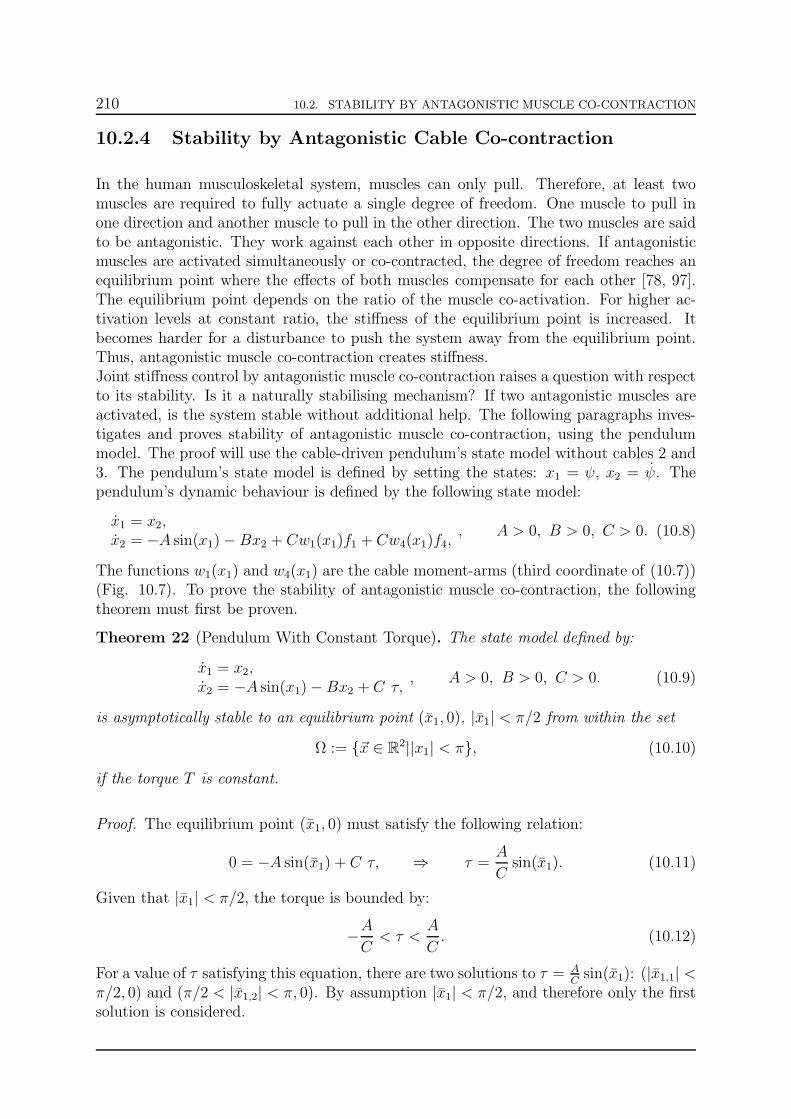
210 10.2. STABILITY BY ANTAGONISTIC MUSCLE CO-CONTRACTION
10.2.4 Stability by Antagonistic Cable Co-contraction
In the human musculoskeletal system, muscles can only pull. Therefore, at least twomuscles are required to fully actuate a single degree of freedom. One muscle to pull inone direction and another muscle to pull in the other direction. The two muscles are saidto be antagonistic. They work against each other in opposite directions. If antagonisticmuscles are activated simultaneously or co-contracted, the degree of freedom reaches anequilibrium point where the effects of both muscles compensate for each other [78, 97].The equilibrium point depends on the ratio of the muscle co-activation. For higher ac-tivation levels at constant ratio, the stiffness of the equilibrium point is increased. Itbecomes harder for a disturbance to push the system away from the equilibrium point.Thus, antagonistic muscle co-contraction creates stiffness.Joint stiffness control by antagonistic muscle co-contraction raises a question with respectto its stability. Is it a naturally stabilising mechanism? If two antagonistic muscles areactivated, is the system stable without additional help. The following paragraphs inves-tigates and proves stability of antagonistic muscle co-contraction, using the pendulummodel. The proof will use the cable-driven pendulum’s state model without cables 2 and3. The pendulum’s state model is defined by setting the states: x1 = ψ, x2 = ψ. Thependulum’s dynamic behaviour is defined by the following state model:
x1 = x2,x2 = −A sin(x1)− Bx2 + Cw1(x1)f1 + Cw4(x1)f4,
, A > 0, B > 0, C > 0. (10.8)
The functions w1(x1) and w4(x1) are the cable moment-arms (third coordinate of (10.7))(Fig. 10.7). To prove the stability of antagonistic muscle co-contraction, the followingtheorem must first be proven.
Theorem 22 (Pendulum With Constant Torque). The state model defined by:
x1 = x2,x2 = −A sin(x1)−Bx2 + C τ,
, A > 0, B > 0, C > 0. (10.9)
is asymptotically stable to an equilibrium point (x1, 0), |x1| < π/2 from within the set
Ω := ~x ∈ R2||x1| < π, (10.10)
if the torque T is constant.
Proof. The equilibrium point (x1, 0) must satisfy the following relation:
0 = −A sin(x1) + C τ, ⇒ τ =A
Csin(x1). (10.11)
Given that |x1| < π/2, the torque is bounded by:
−AC< τ <
A
C. (10.12)
For a value of τ satisfying this equation, there are two solutions to τ = ACsin(x1): (|x1,1| <
π/2, 0) and (π/2 < |x1,2| < π, 0). By assumption |x1| < π/2, and therefore only the firstsolution is considered.

10.2. STABILITY BY ANTAGONISTIC MUSCLE CO-CONTRACTION 211
Consider the following lyapunov candidate for this system:
V (x1, x2) =1
2x22 + A(1− cos(x1)), (10.13)
V (x1, x2) = (C τ − Bx2)x2, (10.14)
The lyapunov candidate satisfies the condition V (~x) < −δ, δ > 0 outside the followingneighbourhood of the origin:
Ω := ~x ∈ R2 | |x1| > π, |x2| >
C |τ |B
. (10.15)
The maximum value of V (~x) on the boundary ∂Ω is:
Vmax(∂Ω) =1
2
(C τ
B
)2
+ 2A. (10.16)
The lyapunov candidate satisfies the condition of uniform boundedness [117]. Thus,system will eventually enter the domain Ω and remain inside the domain. Furthermore,as stated previously, there are at most two fixed points inside Ω, given a value of τsatisfying (10.12). The point (|x1| < π/2, 0) ∈ Ω is a stable centre.The state model defined by (10.9) is asymptotically stable to an equilibrium point (x1, 0),|x1| < π/2 from within the set Ω.
This theorem is used to prove the stability of muscle co-contraction.
Theorem 23 (Antagonistic Cable Co-contraction Stability). The pendulum’s state model(10.8) is locally asymptotically stable to the point (x1, 0), |x1| < π
3, within the set
Ω∗ := ~x ∈ R2||x1| <
π
2, (10.17)
by imposing the cable tensions f1 and f4 to be fixed at constant values
f1 = f1 = cte ≥ 0, f4 = f4 = cte ≥ 0, (10.18)
such that −A sin(x1) + Cw1(x1)f1 + Cw4(x1)f4 = 0. Furthermore, the moment-armfunctions are assumed to have opposite signs (Antagonist muscles).
w1(x1) < 0, and w4(x1) > 0, ∀x1 ∈]−π
2,π
2[. (10.19)
Proof. The first point to observe is that given the geometry of the system the moment-arm functions w1(x1) and w4(x1) are bounded functions. The cable attachment pointsare defined such that in the pendulum frame R1, ∀x1 ∈]− π
2, π2[, cable 1’s force direction
vector ~b1,1 is always in quadrant II of the pendulum’s xy plane. Cable 2’s force direction
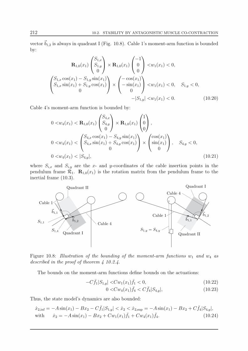
212 10.2. STABILITY BY ANTAGONISTIC MUSCLE CO-CONTRACTION
vector~b1,2 is always in quadrant I (Fig. 10.8). Cable 1’s moment-arm function is boundedby:
R1,0(x1)
S1,x
S1,y
0
×R1,0(x1)
−100
<w1(x1) < 0,
S1,x cos(x1)− S1,y sin(x1)S1,x sin(x1) + S1,y cos(x1)
0
×
− cos(x1)− sin(x1)
0
<w1(x1) < 0, S1,y < 0,
−|S1,y| <w1(x1) < 0. (10.20)
Cable 4’s moment-arm function is bounded by:
0 <w4(x1) < R1,0(x1)
S4,x
S4,y
0
×R1,0(x1)
100
,
0 <w4(x1) <
S4,x cos(x1)− S4,y sin(x1)S4,x sin(x1) + S4,y cos(x1)
0
×
cos(x1)sin(x1)
0
, S4,y < 0,
0 <w4(x1) < |S4,y|, (10.21)
where Si,x and Si,y are the x- and y-coordinates of the cable insertion points in thependulum frame R1. R1,0(x1) is the rotation matrix from the pendulum frame to theinertial frame (10.3).
Quadrant II
Quadrant II
Cable 1
Cable 1
Cable 4
Cable 4
~b1,1
~b1,1 ~b1,2~b1,2
Quadrant I
Quadrant IS1,y = S4,y
S1,1
S1,4
Figure 10.8: Illustration of the bounding of the moment-arm functions w1 and w4 asdescribed in the proof of theorem 4 10.2.4.
The bounds on the moment-arm functions define bounds on the actuations:
−Cf1|S1,y| <Cw1(x1)f1 < 0, (10.22)
0 <Cw4(x1)f4 < Cf4|S4,y|, (10.23)
Thus, the state model’s dynamics are also bounded:
x2,inf = −A sin(x1)− Bx2 − Cf1|S1,y| < x2 < x2,sup = −A sin(x1)− Bx2 + Cf4|S4,y|,with x2 = −A sin(x1)−Bx2 + Cw1(x1)f1 + Cw4(x1)f4. (10.24)

10.2. STABILITY BY ANTAGONISTIC MUSCLE CO-CONTRACTION 213
By theorem 4, the bounding dynamics are stable. The lower bound is asymptoticallystable to the equilibrium point (x1,inf, 0) with −π/2 < x1,inf ≤ 0 from within Ω = ~x ∈R
2||x1| < π. The upper bound is asymptotically stable to the equilibrium point (x1,sup, 0)with 0 ≤ x1,sup ≤ π/2 from within Ω = ~x ∈ R
2||x1| < π.The stability of the bounding dynamics imposes the following on the cable tensions:
0 ≤ f1 <A
C|S1,y|, S1,y 6= 0, 0 ≤ f4 <
A
C|S4,y|, S4,y 6= 0. (10.25)
The insertion points S1,1 and S1,4 of the cables are such that S1,y = S4,y (symmetry).
Furthermore, relations (10.22), (10.23) and (10.25) define:
−A < Cw1(x1)f1 < 0, 0 < Cw4(x1)f4 < A. (10.26)
For equilibrium points (x1, 0), |x1| < π/2, the following relation is defined:
− A sin(x1) + Cw1(x1)f1 + Cw4(x1)f4 = 0,
⇒ Cw1(x1)f1 + Cw4(x1)f4 = A sin(x1),
⇒ −A < Cw1(x1)f1 + Cw4(x1)f4 < A, ∀x1 ∈]−π
2,π
2[ (10.27)
Relations (10.26) and (10.27) agree with each other and impose:
−A < Cw1(x1)f1 + Cw4(x1)f4 < A. (10.28)
The actuation generated by the co-contraction is bounded. Through theorem 4, thesystem is stable to the equilibrium point (x1, 0) with −π/2 < x1 ≤ π/2 from withinΩ = ~x ∈ R
2||x1| < π. Therefore, the system is asymptotically stable to the equilibriumpoint (x1, 0) with −π/3 < x1 ≤ π/3 from within Ω∗ = ~x ∈ R
2||x1| < π/2.
The previous theorem proves that by activating antagonistic cables, the system isstabilised to an equilibrium point. The value of the equilibrium point depends on theratio between the cable tensions and the tensions are limited to a maximum value. Thecable tensions can be changed without changing the equilibrium point if the ratio betweencable tensions remains constant (Fig. 10.9).
10.2.5 Joint Stiffness Control
Thus far, the term ”stiffness” has been used without a formal definition. Stiffness gen-erally defines the relation between force and displacement applied to an object. In aspring, it characterises the amount of force ∆f required to stretch or compress the springby ∆l. In structural engineering it characterises the change in geometry or deflection(angle ∆ϑ or length ∆d) of the structure under an applied force ∆f . In material scienceit characterises the amount of deformation ∆ǫ of the material under a given load ∆σ.The common point between all of these different definitions of stiffness is that when the

214 10.2. STABILITY BY ANTAGONISTIC MUSCLE CO-CONTRACTION
0 1 2 3 4 5 60
1
2
3
4
5
6
−60
−40
−20
0
20
40
0 0.5 1 1.5 2−60
−40
−20
0
20
40
60
0 0.5 1 1.5 2−60
−40
−20
0
20
40
60
0 0.5 1 1.5 2−60
−40
−20
0
20
40
60
Cable force f1 [N] Time t [s]
ψψ
ψ
Cable
forcef 2
[N]
Equilibrium
point:ψ
[deg]
1.1.
f1 = 3, f2 = 6
2.
2.f1 = 3, f2 = 3
3.3. f1 = 4, f2 = 1
ψ = 48
ψ = 0
ψ = −33
Figure 10.9: Illustration of the equilibrium point achieved by antagonistic cable co-contraction as described by theorem 5, section 10.2.4.
force or load is removed, the spring, structure or material returns to its original state.Stiffness characterises a behaviour that is reversible or elastic.Stiffness is mathematically defined as the infinitesimal change in external action over theinfinitesimal change in internal reaction.
K =∂χ
∂q,
χ : force f / load σ,q : displacement l / deflection d/ deformation ǫ.
(10.29)
In this chapter, joint stiffness is defined as the required infinitesimal change in joint torqueτ to impose an infinitesimal change in joint configuration ψ.
K =∂τ
∂ψ,
τ : torque on pendulum axis,ψ : pendulum angle.
(10.30)
For the complete cable-driven mechanism (all four cables), the stiffness normalised bythe inertia, is defined by:
K(x1) =∂x2∂x1
= −A cos(x1) + C∂W(x1)
∂x1~f. (10.31)
The stiffness around an equilibrium point x1 is K(x1). For a given muscle activationlevel, the stiffness is governed by moment-arms. The first term in the previous relation isfrom the system’s dynamics. The second term is from the cable structure. Once the forceactivation levels are set, the stiffness depends on the internal dynamics and moment-arms. For there to be stability, the moment-arms must be the governing term. Themuscle co-contraction must control the stiffness and not the system’s dynamics.
Human motor control uses the muscle activation levels to actively change the prop-erties of the joint in terms of stiffness and configuration. Joint stiffness control by an-tagonistic muscle co-contraction changes the activation levels of the muscles to achieve a

10.2. STABILITY BY ANTAGONISTIC MUSCLE CO-CONTRACTION 215
desired characteristic.There are two distinct methods of using the antagonistic muscles. At constant ratio,the muscle forces can be changed to produce more or less stiffness without changing theequilibrium point. This is called iso-equilibrium stiffness control (Fig. 10.10). The mus-culature can actively control the stiffness to deal with the external perturbations. Atconstant stiffness, the equilibrium point can be changed. The activation ratio is changedsuch that the equilibrium point changes but not the stiffness. This is called iso-stiffnessequilibrium control. In general situations, the stiffness and equilibrium point are contin-uously changed.
0 1 2 3 4 5 60
1
2
3
4
5
6
0 1 2 3 4 5 60
1
2
3
4
5
6
0
2
4
6
8
10
12
14
16
Cable force f1 [N]Cable force f1 [N]
Cable
forcef 2
[N]
Cable
forcef 2
[N]
Iso-stiffness equilibrium point change
Iso-equilibrium point stiffness change
Equilibrium Stiffness Contours K(x1) Iso-Stiffness / Iso-Equilibrium
Figure 10.10: Illustration of the equilibrium stiffness and the relation between iso-stiffnessand iso-equilibrium lines 10.2.4.
10.2.6 Observability of Pendulum States
Joint stiffness control relies on knowledge of the joint’s position. In section 10.2.1, it isstated that the nervous system measures primarily each muscle’s length, rate of changeand activation level. There is another type of nerve cell that measures information re-garding the joints, called mechanoreceptor. Mechanoreceptors are known to measuremechanical deformation. There are other types of mechanoreceptors in our skin that giveus a sense of touch. Golgi tendon organs are also a type of mechanoreceptor. However, itis unclear if joint mechanoreceptors relay information regarding each joint’s current con-figuration [177]. Therefore, this section shows that the joint’s position can be measuredor observed through the measure of muscle length and rate of change.
As stated in section 10.2.1, the nervous system measures the muscle lengths Li andthe rates of changes in each length Li. Therefore, are the pendulum states x1 and x2observable through the cable lengths Li and rates Li? The short answer is yes, but theobservability will be formally proven.

216 10.2. STABILITY BY ANTAGONISTIC MUSCLE CO-CONTRACTION
Theorem 24 (Observability of Pendulum States). The states of the following dynamicsystem
x1 = x2, (10.32)
x2 = −A sin(x1)−Bx2 + CW(x1)~f, (10.33)
are observable through the output function defined by:
~y(x1, x2) =(
L1 L2 L3 L4 L1 L2 L3 L4
)T, (10.34)
Proof. The proof involves showing the observability matrix is full column rank. Thematrix is constructed from a linearisation around an arbitrary equilibrium point ~yc =
(x1, 0), |x1| ≤ π3. The vector ~f is the cable force distribution at the equilibrium point.
−A sin(x1) + CW(x1) ~f = 0. (10.35)
The linearised pendulum model is defined by:
x1 ≈ x2, (10.36)
x2 ≈(
−A cos(x1) + C∂W
∂x1
∣∣∣∣x1=x1
~f
)
x1 −Bx2 + CW(x1)~f, (10.37)
The state matrices A and B are defined by:
A =
0 1(
−A cos(x1) + C ∂W∂x1
∣∣∣x1=x1
~f
)
−B
, B =
(0
CW(x1)
)
(10.38)
The output function ~y(x1, x2) is also linearised around the equilibrium point:
~y(x1, x2) ≈
L1...L4
˙L1...˙L4
+
∂L1
∂x1
∣∣∣x1,0
0
......
∂L4
∂x1
∣∣∣x1,0
0
∂L1
∂x1
∣∣∣x1,0
∂L1
∂x2
∣∣∣x1,0
......
∂L4
∂x1
∣∣∣x1,0
∂L4
∂x2
∣∣∣x1,0
(x1x2
)
= ~y(x1, 0) +C
(x1x2
)
. (10.39)
The states x1 and x2 are locally observable if and only if the observability matrix O has

10.3. A JOINT STIFFNESS CONTROL STRATEGY 217
full column rank. The observability matrix is defined for this particular model by:
O =
(C
CA
)
=
∂L1∂x1
∣
∣
∣
x1,00
......
∂L4∂x1
∣
∣
∣
x1,00
∂L1∂x1
∣
∣
∣
x1,0
∂L1∂x2
∣
∣
∣
x1,0
......
∂L4∂x1
∣
∣
∣
x1,0
∂L4∂x2
∣
∣
∣
x1,0
0∂L1∂x1
∣
∣
∣
x1,0
......
0∂L4∂x1
∣
∣
∣
x1,0
∂L1∂x2
∣
∣
∣
x1,0A2,1,
∂L1∂x1
∣
∣
∣
x1,0+
∂L1∂x2
∣
∣
∣
x1,0A2,2
......
∂L4∂x2
∣
∣
∣
x1,0A2,1,
∂L4∂x1
∣
∣
∣
x1,0+
∂L4∂x2
∣
∣
∣
x1,0A2,2
≡
×1 0×2 0×3 0×4 0× ×× ×× ×× ×0 ⋆10 ⋆20 ⋆30 ⋆4× ×× ×× ×× ×
. (10.40)
The observability matrix is full column rank (rank = 2) for any equilibrium point ~yc =(x1, 0), |x1| ≤ π
3. Indeed, the first four rows have a single non-zero element (×i). Rows
9 to 12 also have a single non-zero element (⋆i). The non-zero elements are in differentcolumns. Furthermore, the elements are equal to each other in pairs of two (×i = ⋆i,i = 1, 2, 3, 4). These elements are never zero on the interval x1 ∈]−π/3, π/3[ (Fig. 10.7).Thus, as long as at least one of these elements is non-zero, the matrix is guaranteed tohave full column rank. Therefore, the states x1 and x2 or ψ and ψ are observable throughthe cable lengths Li and rates Li.
This theorem proves that the state of the pendulum can be known through the lengthsand rates of change in length of each cable. It is therefore hypothesised that the nervoussystem does know the state of each joint using the measured muscle states and theinformation from the mechanoreceptors [169].
10.3 A Joint Stiffness Control Strategy
Thus far, the general function of human motor control has been presented and the mech-anism of joint stiffness control through antagonistic muscle co-contraction has been pre-sented and analysed. The findings are that antagonistic muscle co-contraction producesmore or less stiffness around an equilibrium point and the equilibrium point dependson the muscle activation levels. Furthermore, muscle co-contraction yields a stabilisingeffect around the equilibrium point. The equilibrium point is stable. Meaning, if theskeletal system is pushed away from the equilibrium point by a disturbance, the muscleco-contraction pushes it back to the equilibrium in the same way a spring would.It was also shown that muscle moment-arms govern the stability around the equilibrium

218 10.3. A JOINT STIFFNESS CONTROL STRATEGY
point. Once the muscle activation levels are set, the moment-arms govern the actuation.Muscle moment-arms play an important role in that they relate skeletal dynamics to mus-cle forces. In musculoskeletal modelling, moment-arms are used to estimate the muscleforces, given desired skeletal dynamics. Thus, the hypothesis put fourth by this chapterconcerning a possible neuromuscular dysfunction causing osteoarthritis is the following.A deterioration in the nervous system’s knowledge of the moment-arms can lead to ex-cessive muscle forces. This in turn causes excessive joint forces. There is some form ofmismatch between the actual system and the nervous system’s perception of the system.
The following sections present and discuss how a mismatch between the system’smoment-arms and the moment-arms perceived by the controller can induce excessivejoint loading through joint stiffness control. If a mismatch is inserted into the joint stiff-ness control mechanism, excessive muscle forces are generated and therefore excessivejoint forces are generated. To illustrate this point, a joint stiffness control strategy is firstproposed for the cable-driven pendulum. The strategy is then implemented onto the realsystem and tests are run using biased and unbiased moment-arms.The reason for investigating moment-arms is that they are the primary quantity describ-ing the musculature’s ability to actuate the skeletal system. If the moment-arms arenot computed correctly, the coordination strategy will yield inappropriate muscle forces.This point was previously illustrated in chapter 8. A poor definition of the shouldermodel’s muscle wrapping yielded inappropriate muscle activation patterns and overesti-mated joint reaction forces. There is another less obvious reason for investigating theeffect of biased moment-arms. In control in general, there are a number of reason’s whya controller can generate inappropriate input patterns. However, in many situations theresult is instability. Therefore, the fact that biased moment-arms leads to inappropriatemoment-arms without loss of stability is relevant because osteoarthritis is a dysfunctionwithout loss of stability.
10.3.1 Control Algorithm
This section proposes a strategy of using muscle co-contraction to actively control andstabilise the cable-driven pendulum. The general concept of the strategy is to impose astiffness and compute the required forces by solving the cable-force coordination problempresented in chapter 7. In the previous section only two cables were considered. Theproposed strategy uses all four cables for more flexibility. The required torque on thependulum’s axis is produced by four cables thereby reducing the intensity in each cable.To impose a stiffness on the system, around an equilibrium point (x1, 0), is to impose thefollowing behaviour on the pendulum’s dynamics.
x2 = −A sin(x1)−Bx2+CW(x1)~f = −A sin(x1)−Bx2+Ks(x1−x1)+A sin(x1), (10.41)
where Ks > 0 is the imposed stiffness. The stiffness around any equilibrium point (x1, 0)is defined by:
K(x1) =∂x2∂x1
∣∣∣∣x1=x1
=
(
−A cos(x1) + C∂W(x1)
∂x1~f
)∣∣∣∣x1=x1
= −A cos(x1) +Ks. (10.42)

10.3. A JOINT STIFFNESS CONTROL STRATEGY 219
where ~f is the vector of muscle forces associated to the equilibrium point.
The proposed strategy is an iso-stiffness strategy. The stiffness coefficient is selectedand remains constant. The following theorem proves that such a strategy is stable forthe pendulum system.
Theorem 25. The dynamical system defined by the following state model:
x1 = x2,x2 = −A sin(x1)− Bx2 + Cu,
A > 0, B > 0, C > 0, (10.43)
is locally asymptotically stable to the point ~x = (x1, 0), |x1| < π, within the set
Ω := ~x ∈ R2||x1| < π, (10.44)
using the control law
u = Ks(x1 − x1) +A
Csin(x1), Ks > B > 0. (10.45)
Proof. The proof involves showing that a suitable lyapunov candidate satisfies the con-ditions of theorem 1 in chapter 9. To prove asymptotic stability of the system within thedomain Ω, the following variable change is defined
y1 = x1 − x1 −A
CKs
sin(x1) = x1 − x∗1,
y2 = x2,⇒y1 = y2,y2 = −A sin(y1 + x∗1)− C(Ksy1 +By2).
(10.46)
Consider the lyapunov candidate
V (~y) =1
2~yTP~y + A(1− cos(y1 + x∗1)), (10.47)
where the matrix P is symmetric positive definite [117].
P =
(p11 p12p12 p22
)
, p12 > 0, p11p22 − p212 > 0. (10.48)
Given that A > 0 by assumption and P is symmetric positive definite, the functionV (~y) > 0, ∀~y ∈ R
2. The time derivative of the function is defined by:
V (~y) =~yTP~y + Ay2 sin(y1 + x∗1)),
=2 (p12 −Kdp22) y22 − 2Ksp12y
21 + 2 (p11 −Kdp12 −Ksp22) y1y2+
(y2 − 2p12y1 − 2p22y2) sin(y1 + x∗1). (10.49)
By selecting p11 =CKs
2+ (CB)2
4, p12 =
CB4
and p22 =12, the expression of V reduces to
V (~y) = −1
2
(C2KsBy
21 + CBy22 + ACBy1 sin(y1 + x∗1)
). (10.50)
This function is negative definite within the set:
Ωy := ~y ∈ R2||y1 + x∗1| < π, (10.51)

220 10.3. A JOINT STIFFNESS CONTROL STRATEGY
The interval is valid because the term x∗1 = x1 +A
CKssin(x1) has the same sign as x1 over
the interval |x1| < π. Furthermore, the derivative is equal to zero for ~y = (0, 0). Thus,(10.46) is asymptotically stable to ~0 in Ωy and therefore (10.43) is asymptotically stableto (x1, 0) in Ω using the control law (10.45).
Given a stiffness KS and equilibrium point x1 the cable tensions must produce thedesired input. The desired behaviour is ~yc = (x1, 0). The outputs of the system are thestates ~y = (x1, x2). The cable-tension must satisfy the following relation which is theprimary task:
u = K(~yc − ~y) =
(
Ks(x1 − x1) +A
Csin(x1)
)
= W~f (10.52)
Furthermore, the desired behaviour must be within the wrench feasibility space imposedby the strength limits of each cable. The cable tensions are obtained using the samestrategy as chapter 7. The coordination strategy is defined as an optimisation problemto find a solution minimising the cable tensions. This is the secondary task. The costfunction is the sum of cable forces squared. The primary task is defined as an equalityconstraint. Bounds are also set on the tensions. Cables can only pull and have a maximumtensile strength. The coordination strategy is thus defined by:
min~f
Γ(~f) =1
2~fT ~f, Secondary Task, (10.53)
s.t.
(
Ks(x1 − x1) +A
Csin(x1)
)
= W~f, Control Law, Primary Task, (10.54)
~0 ≤ ~f ≤ ~fmax, Min/Max Tensions Bounds. (10.55)
This coordination strategy can be solved using the same null-space optimisation approachas defined in chapter 7. A pseudo-inverse of the moment-arms matrix yields a solutionminimising the cable tensions while satisfying the control law constraint.
~f ∗ = WT(WWT
)−1(
Ks(x1 − x1) +A
Csin(x1)
)
. (10.56)
The solution is then corrected using the null-space of the moment-arm matrix to satisfythe bounds on the cable-tensions.
~f = ~f ∗ +N~v, WN = 0. (10.57)
This parameterisation of the problem yields a quadratic program (cf. chapter 7).
min~v
Γ(~v) =1
2~vTNTN~v +
1
2
(
~f ∗)T
N~v, (10.58)
s.t. N~v ≤ ~fmax − ~f ∗, (10.59)
−N~v ≤ ~f ∗. (10.60)
Thus, the control algorithm is stated in the form of a theorem. A damping factor Kd isincluded into the control law to have more flexibility. This does not change the stability aslong asKS > Kd+B > 0 andKd > 0. There is no proof, given that the previous theoremsand proofs have already defined its stability. Lastly, wrench-feasibility is assumed.

10.3. A JOINT STIFFNESS CONTROL STRATEGY 221
Theorem 26 (Joint Stiffness Control Algorithm). The following dynamic system:
x1 = x2, (10.61)
x2 = −A sin(x1)−Bx2 + CW(x1)~f, (10.62)
~y = (x1, x2)T , (10.63)
is locally asymptotically stable to the point ~yc = (x1, 0), |x1| ≤ π3, within the set
Ω := ~x ∈ R2||x1| < π, (10.64)
using the control law
u = K(~yc − ~y) =
(
Ks(x1 − x1)−Kdx2 +A
Csin(x1)
)
= W~f (10.65)
where ~f is defined by
~f = ~f ∗ +N~v, ~f ∗ = WT(WW
T)−1(
Ks(x1 − x1)−Kdx2 +A
Csin(x1)
)
.
(10.66)
The vector ~f is found through the quadratic program
min~v
Γ(~v) =1
2~vTNT
N~v +1
2
(
~f ∗)T
N~v, (10.67)
s.t. N~v ≤ ~fmax − ~f ∗, (10.68)
−N~v ≤ ~f ∗. (10.69)
10.3.2 Implementation
The stiffness control strategy was implemented on a physical system (Fig. 10.11). Thephysical system is exactly like the model presented in section 10.2.3. The pulleys aredriven by brushless EC motors through a planetary gear head with a gear of ratio Ng
(Fig. 10.8). The electric motors are driven in current Ii and can be viewed as idealtorque sources. The pulleys have an inertia Jp. The motor’s have inertia’s Jm and thereis friction T (ϑi). The friction on the real system is hypothesised to behave according tothe kinetic friction model [4].
τ(ϑi) = σ2ϑi + σ0g(ϑi)sign(ϑi) +(
1− |sign(ϑi)|)
sat(NgkIi, τs), (10.70)
σ0g(ϑi) = τs exp(−ϑ2i /νs) + τc
(
1− exp(−ϑ2i /νs))
. (10.71)

222 10.3. A JOINT STIFFNESS CONTROL STRATEGY
where τs is the static friction torque, τc is the kinetic friction, νs the Stribeck curvecoefficient. sign(θi) is the sign usual sign function. sat(Ii, Ts) is a saturation functionthat switches between the current input being applied and the static friction force. Allthe coefficients were identified on the real system using the appropriate techniques [4].
ϑ1
ϑ2ϑ3
ϑ4
ψ
CAD Drawning
Frame
Real System
∼500[m
m]
∼ 400 [mm]
Schematic of drive-train
R1
R2
Motor 1
Motor 2Motor 3
Motor 4
Ng
Power Source
Amplifier
EC Brushless motor
Pulley Inertia Jp
Planetary Gearhead
ϑm,i
ϑi
Motor Inertia Jm
Friction T (ϑi)
Figure 10.11: Illustration of the physical system and schematic of the drive train asdescribed in section 10.3.3.
The motors are used to generate tension fi within each cable and actuate the system.A dynamic state model is constructed for each pulley. The states are defined as the anglex1,i = ϑi and angular velocity x2,i = ϑi. The inputs are the motor currents ui = Ii.
x1,i = x2, (10.72)
x2,i =1
(N2gJm + Jp
)(−N2
g τ(x2,i) +NgkIi − rfi), i = 1, 2, 3, 4, (10.73)
The parameter k is the ideal torque source proportionality constant. A state model isbuilt for the entire system by selecting the states and inputs as follows.
~x : x1 = ψ, x1,1 = ϑ1, ..., x1,4 = ϑ4, x2 = ψ, x2,1 = ϑ1, ..., x2,4 = ϑ4,~u : u1 = I1, u2 = I2, u3 = I3, u4 = I4.
All states are measured on the real system using angular encoders. The motor currentsare also measured. The resulting model is a non-linear affine in the input state model:

10.3. A JOINT STIFFNESS CONTROL STRATEGY 223
~x = ~f(~x) + ~g(~x)~u.
~x =
x1 = x2x1,1 = x2,1x1,2 = x2,2x1,3 = x2,3x1,4 = x2,4x2 = −A sin(x1)−Bx2 + CW(x1)~fx2,1 = D · τ(x2,1) + F · f1 +G · u1x2,2 = D · τ(x2,2) + F · f2 +G · u2x2,3 = D · τ(x2,3) + F · f3 +G · u3x2,4 = D · τ(x2,4) + F · f4 +G · u4
A = 4 MpglpIp+Ml2p
B = 4 bpIp+Ml2p
C = 4 1Ip+Ml2p
D = − 1N2
gJm+Jp
F = − rN2
gJm+Jp
G = Ngk
N2gJm+Jp
(10.74)
Given that each motor is equipped with an encoder, the length of each cable can becomputed using the pulley angles ϑi. The pendulum is initially at an angle ψ0 (= 0 bydefault). The initial length Li(ψ0) of each cable is known using method the geometricmethod described in section 10.2.3. The pulley angles are all initially zero and the cablesare assumed to always remain taught. Once the pendulum begins to move, the length ofeach cable is computed using the following relation.
Li = Li(ψ0) + rϑi, i = 1, 2, Li = Li(ψ0)− rϑi, i = 3, 4. (10.75)
The sign is different for cables three and four because the pulley angle is positive whenthe cable’s length is decreasing.
The joint stiffness control algorithm presented in the previous section is implementedfor tracking a reference behaviour ~yc = (x1, 0). The control algorithm yields the necessarycable tensions fi that each motor must produce. The motor currents were obtained byassuming that the pulley accelerations x2,i are equal to the desired accelerations x2,i,c.This assumption allows one to define the motor inputs as:
ui =1
G(x2,i,c − αD · τ(x2,i)− F · fi) , i = 1, 2, 3, 4. (10.76)
The friction term is incorporated into the control law. This is called friction compen-sation by positive feedback. The coefficient 0 < α < 1 is such that the friction termdoes not destabilise the system and is tuned by hand. Friction compensation is essentialbecause planetary gear heads are prone to large amounts of friction.The control algorithm was implemented using the assumption that the pendulum statesare known and need not be observed. An Luenberger observer was designed and imple-mented but the observer states were not used for control (cf. chapter 9). The observerwas designed for illustration purposes with respect to the discussion of section 10.2.6 onthe observability of joint states through the muscle states. The observer is not performantenough to use in a control strategy.
The state variables on the physical system are measured using angular encoders. Thereis an angular encoder on each motor with a precision of 0.7 (512 counts per turn). Onthe pendulum itself there is an angular encoder with a precision of 0.08 . The inputs are

224 10.3. A JOINT STIFFNESS CONTROL STRATEGY
also measured. Each motor is controlled by an operational amplifier that also measuresthe amount of current being applied to each motor. The implantation is done using asampling rate of 80Hz (Measurements are taken 80 times a second and inputs are sentto the system 80 times a second). Finally, the control algorithm was implemented by
imposing a minimum tension ~fmin > 0. This ensures that the cables remain taught.
10.3.3 Methods
To analyse the effect of biased moment-arms on the joint reaction force in the jointstiffness control strategy, the system was programmed to track a reference signal thatswitches between constant values at regular intervals. Each switch is defined using atransition function that smoothly changes the reference value. This avoides any suddenjump in motor current that would yank on the cables and cause damage to the mechanism.The transition function ξ(t, ψA, ψB) is defined by the following polynomial function. Theinitial time is always defined as t0 = 0 and the final time T can be modulated to imposemore or less dynamics.
ξ(t, x1,A, x1,B) = x1,A +
5∑
i=1
pi(x1,B − x1,A)
(t− t0T − t
)i
. (10.77)
The coefficients pi of the polynomial are obtained by imposing the following initial andfinal conditions:
ξ(t0, x1,A, x1,B) = x1,A,ξ(T, x1,A, x1,B) = x1,B
,ξ(t0, x1,A, x1,B) = 0,
ξ(T, x1,A, x1,B) = 0,
ξ(t0, xT,A, x1,B) = 0,
ξ(T, x1,A, x1,B) = 0.(10.78)
The order of the polynomial function is set at five but other orders can be used. Higherorders allow one to have greater control over the behaviour. The order five is selectedbecause it yields a sufficiently smooth behaviour.
The reference signal uses most of the pendulum’s angular space. In section 10.2.3 itwas stated that the pendulum can swing in the interval ±75. The reference signal isdefined with an amplitude range of ±60. The constant values are defined at 0, ±30
and 60.
During one cycle of the reference trajectory, the pendulum’s states are measuredthrough an encoder. The states of each motor and the amount of current being appliedto each motor are measured. The currents are proportional to the forces within eachcable and are used to compute the reaction force in the pendulum’s axis.To analyse the effect of stiffness control on the joint reaction force, the system was setto track the desired path using three settings of the moment arms. First, the path wastracked using nominal values of the moment-arms. Second, the path was tracked usingmoment-arms that were underestimated by 20%. Third, and last, the path was trackedusing moment-arms that were 20% overestimated.
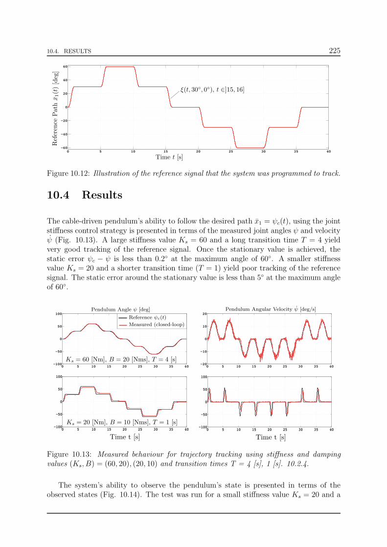
10.4. RESULTS 225
0 5 10 15 20 25 30 35 40−60
−40
−20
0
20
40
60
Reference
Pathx1(t)[deg]
Time t [s]
ξ(t, 30, 0), t ∈]15, 16]
Figure 10.12: Illustration of the reference signal that the system was programmed to track.
10.4 Results
The cable-driven pendulum’s ability to follow the desired path x1 = ψc(t), using the jointstiffness control strategy is presented in terms of the measured joint angles ψ and velocityψ (Fig. 10.13). A large stiffness value Ks = 60 and a long transition time T = 4 yieldvery good tracking of the reference signal. Once the stationary value is achieved, thestatic error ψc − ψ is less than 0.2 at the maximum angle of 60. A smaller stiffnessvalue Ks = 20 and a shorter transition time (T = 1) yield poor tracking of the referencesignal. The static error around the stationary value is less than 5 at the maximum angleof 60.
0 5 10 15 20 25 30 35 40−100
−50
0
50
100
0 5 10 15 20 25 30 35 40−20
−10
0
10
20
0 5 10 15 20 25 30 35 40−100
−50
0
50
100
0 5 10 15 20 25 30 35 40−100
−50
0
50
100
Time t [s]Time t [s]
Pendulum Angle ψ [deg] Pendulum Angular Velocity ψ [deg/s]
Reference ψc(t)
Measured (closed-loop)
Ks = 60 [Nm], B = 20 [Nms], T = 4 [s]
Ks = 20 [Nm], B = 10 [Nms], T = 1 [s]
Figure 10.13: Measured behaviour for trajectory tracking using stiffness and dampingvalues (Ks, B) = (60, 20), (20, 10) and transition times T = 4 [s], 1 [s]. 10.2.4.
The system’s ability to observe the pendulum’s state is presented in terms of theobserved states (Fig. 10.14). The test was run for a small stiffness value Ks = 20 and a

226 10.5. DISCUSSION
0 5 10 15 20 25 30 35 40−100
−50
0
50
100
0 5 10 15 20 25 30 35 40−500
−250
0
250
500
Time t [s]Time t [s]
Pendulum Angle ψ [deg] Pendulum Angular Velocity ψ [deg/s]
Ks = 20 [Nm], B = 10 [Nms], T = 1 [s]
Reference ψc(t)
Observed (closed-loop)Measured (closed-loop)
Figure 10.14: Observed pendulum states over one cycle of the path ψc(t) with stiffnessand damping values: Ks = 20 [Nm], B = 10 [Nms]. The transition time was set at T = 1[s].
short transition time. The observed pendulum angle follows the measured angle quite wellconsidering the nature of the observer. At every change in static angle, there is a smallovershoot of the observed angle. There is a static error of less than 4 at the maximumangle of 60 between the measured angle and the observed angle. The observed velocityhas an extremely large overshoot and does not converge to a steady state before the nextstep. The observed velocity does tend towards the measured value but convergence to astatic value is not observed.
The required tensions within the cables were observed through the currents in themotors (Fig. 10.15). The maximum cable tensions were observed when the right/leftcables had to pull the pendulum towards them at ±60 (t = 10 and t = 30 [s]). Thetwo outer cables were observed to pull harder than the two inner cables. Larger cabletensions were required for faster transition times and higher stiffness values.
The effect of using over or underestimated moments-arms is a decrease or increasein joint reaction force by the same amount (Fig. 10.16). It was observed that a 20%increase in moment-arms lead to a 20% decrease in joint reaction force. Vice-versa, a20% decrease in moment-arms results in a 20% increase in joint reaction force. Thisaffect was most prominently observed when the cables had to pull the hardest.
10.5 Discussion
In the introduction, it was stated that osteoarthritis could be caused by an underlyingneuromuscular dysfunction. The observed cause is frequent excessive loading of the ar-ticular cartilage leading to premature deterioration. However, the source of the excessiveloading has not been identified [16]. The neuromuscular dysfunction hypothesis resultsfrom the following reasoning. A musculoskeletal system is a tensegrity system [188]. Themuscles are in tension and the bones are in compression. The compression results fromthe muscles contracting. The contraction results from neural stimuli. Thus, the neu-romuscular dysfunction hypothesis is that the neural stimuli are causing inappropriate

10.5. DISCUSSION 227
0 10 20 30 400
10
20
30
40
50
60
0 10 20 30 400
20
40
60
80
100
120
0 10 20 30 400
20
40
60
80
100
120
140
0 10 20 30 400
10
20
30
40
50
60
70
Time t [s]Time t [s]
Time t [s]Time t [s]
Cable
Ten
sionf1[N
]
Cable
Ten
sionf2[N
]
Cable
Ten
sionf3[N
]
Cable
Ten
sionf4[N
]
Figure 10.15: Estimated cable tensions during one cycle of the path ψc(t). These tensionsare for a stiffness of Ks = 20 [Nm], a damping factor of B = 10 [Nms]. The transitiontime was set at T = 1 [s].
muscle contraction leading to excessive loads in the joints. Osteoarthritis is a neuralcontrol problem.The part of our nervous system controlling our musculoskeletal system is called humanmotor control. Within human motor control is a mechanism called joint stiffness controlthrough antagonistic muscle co-contraction. Our musculature is setup such that certainmuscles act as opposites. The nervous system activates or co-contracts these muscles togive the joints variable stiffness. The findings of this chapter show that such a mechanismcan contribute to excessive loads in the joints. The findings of this chapter are obtainedusing a model of a cable-driven pendulum. Although the model is not that of a muscu-loskeletal system, the results are relevant. Indeed, the model is mathematically identicalto a model of a musculoskeletal system. Models of cable-driven mechanisms and modelsof musculoskeletal systems are based on the same set of principles.
The chapter used a simplified model of neuromuscular interactions where the nervoussystem measures each muscle’s length, rate of change in length and muscle activationlevel. This information was also shown to contain the state of the joints using the con-cept of observability from control theory. Therefore, the nervous system is assumed tohave full knowledge of the dynamic state of the skeletal system [169]. Furthermore, itis believed that the nervous system has a model of the musculoskeletal system [177]. It

228 10.5. DISCUSSION
0 5 10 15 20 25 30 35 400
50
100
150
200
250
8 10 120
50
100
150
200
250
18 20 220
20
40
60
80
100
28 30 320
50
100
150
200
Time t [s]Time t [s]Time t [s]
Time t [s]
I.
I.
II.
II.
III.
III.
Pen
dulum
ReactionForcefr[N
]Pen
dulum
ReactionForcefr[N
]
Underestimatedmomen
t-arm
s
Unbiasedmomen
t-arm
s
Overestimatedmomen
t-arm
s
Figure 10.16: Reaction force in the pendulum rotation axis using nominal, overestimatedand underestimated moment-arms.
uses the model to predict required muscle activation levels.Throughout this dissertation, muscle moment-arms are shown to govern the prediction ofmuscle activation levels (cf. chapter 7). The moment-arms can be obtained using the ten-don excursion method. The moment-arms are defined as the variation in muscle lengthover the variation in joint configuration. Given that both quantities are measured bythe musculoskeletal system, it is highly probable that the nervous system has a measureof the moment-arms. Indeed, this information characterises the musculature’s ability toactuate the skeletal system and produce movement.Based on the hypothesis that moment-arms are measured by the nervous system, exces-sive joint loads are produced if the moment-arms are biased. Predicted muscle activationlevels computed from biased moment-arms yield altered joint loads. Underestimatedmoment-arms lead to excessive joint loads. This point was illustrated through an im-plementation of a joint stiffness control strategy onto a physical cable-driven pendulumsystem. There are many possible dysfunctions of the system that could disturb humanmotor control. Biased moment-arms were selected because they yielded altered jointloads without compromising stability. Loss of stability is not on the list of symptoms ofosteoarthritis. The insertion of delay into the control loop was tested but quickly lead toinstability.

10.6. CONCLUSIONS 229
Finally, the results showed that the use of underestimated moment-arms produces ex-cessive loads without producing instability. This point is important because osteoarthri-tis does not destabilise the musculoskeletal system. Thus, a contributing factor of os-teoarthritis could be biased information regarding the musculoskeletal system, leadingto underestimated muscle moment-arms, leading to excessive muscle forces, leading toexcessive joint forces. This point remains however an unproven conjecture.
10.6 Conclusions
The goal of this chapter was to initiate the investigation of a possible neuromusculardysfunction as the underlying cause of osteoarthritis. The investigation was carried outusing a model of a cable-driven pendulum that is mathematically identical to a modelof a musculoskeletal system. The presentation was set in the context of modern controltheory, using a simple model of the interactions between the musculoskeletal and nervoussystems. The investigation focused on the mechanism of joint stiffness control throughantagonistic muscle co-contraction. The results showed that joint stiffness control is anaturally stabilising mechanism. By activating the antagonistic cables, the pendulumis stabilised to an equilibrium point. The equilibrium point is defined by the ratio ofthe activation levels. The investigation also showed that the joint’s dynamic state can beobserved through the dynamic states of the muscles. An implementation of a joint stiffnesscontrol strategy onto a physical cable-driven pendulum showed that if the controller usesbiased information regarding the cable’s ability to actuate the system, the reaction forcein the joint is increased by a factor proportional to the bias. The use of biased informationdid not however lead to instability. Therefore, joint stiffness control can contribute toexcessive joint loads through antagonistic muscle co-contraction.The results are relevant to the subject of osteoarthritis and open the discussion on thepossible causes but does not provide a definitive answer. The next step of the investigationshould be to use a model of a musculoskeletal system such as the shoulder model presentedin this dissertation. Also an internal muscle model should be added to the shoulder modelto give it more realism.

230 10.6. CONCLUSIONS

Chapter 11
Conclusions
Modelling musculoskeletal systems constitutes a necessary tool for understanding muscu-loskeletal diseases and developing appropriate treatments. Models provide information onthe behaviour of musculoskeletal systems that cannot be directly observed. The develop-ment of such models is a challenging task because of the complexity of the musculoskeletalsystems and because there is no standard validation method.This dissertation presented a musculoskeletal model of the human shoulder. The modelis being developed for the study of osteoarthritis, the most common form of arthritis.Osteoarthritis can be defined as a premature deterioration of the articular cartilage dueto frequent excessive loading. The development of proper treatments for osteoarthritisrequires identifying and estimating the forces in the affected articulations. Given thatthe glenohumeral joint is the shoulder articulation that is most affected by osteoarthritis,the model is being specifically designed to compute the reaction force intensity in theshoulder joint, during quasi-static and dynamic movements of the upper limb.
Two main conclusions can be made from the work presented in this dissertation. Thefirst conclusion is that the reaction force in an articulation is dependent on the movementof the articulation itself and on the movement of other articulations. The parameterisa-tion of the shoulder’s kinematics constitutes the first critical point in estimating the forcein the glenohumeral joint. Muscle forces and joint reaction forces are related throughthe laws of motion from classical mechanics. A muscle activation pattern generates amovement of the skeletal structure and creates a reaction force in the joints. In this dis-sertation, the kinematics are imposed and the corresponding muscle forces are estimatedby inverting the laws of rotation motion. The estimated muscle forces are used to obtainthe reaction force in the glenohumeral joint through the translational laws of motion. Tosum up, for a musculoskeletal model to successfully predict the joint reaction forces, thekinematic model must be able to accurately reproduce the systems movement.The second conclusion is that geometry of the muscle model must be designed by con-sidering all the muscles together. In the real shoulder, muscles are coordinated by thenervous system and produce together the overall result of movement and strength of ourmusculoskeletal system. There have been few analysis of how to use the cable modelfor representing the musculature. The one most referred to in the literature analyses
231

232 11.1. CONTRIBUTIONS
muscles individually and describes how to represent muscles with large attachment sites[197]. This constitutes the first step in constructing the model of the musculature. As asecond step, this dissertation proposes to analyse the model’s wrench-feasibility throughthe moment-arms. In the model, the relation between muscle forces and movement is de-fined by muscle moment-arms. The muscles are geometrically modelled by cables definingmoment-arms around each joint. The force of a cable multiplied by its moment-arm cre-ates a torque at each joint that contributes with the other cable forces to the movementof the system. A model is wrench feasible if it can generate the same set of movementsas the real system.This leads to the third and final conclusion. The articulations of the real system are sta-ble. Stability in this context is understood as keeping the joint reaction force directed atthe surface of the joint. In the real system the muscle-force activation patterns producestable joint force patterns. In the model, the estimated muscle forces should also producestable joint reaction forces, without using constraints. For a musculoskeletal model tosuccessfully predict the joint reaction force pattern, the geometric muscle model mustbe able to accurately reproduce the relation between muscle-forces and movement. Toachieve stable reaction force patterns, the geometric muscle model should be designedas a collective, considering each muscle’s contribution in relation to the others. A goodmusculoskeletal model should naturally produce stable joint reaction force patterns.
11.1 Contributions
The motivation of this thesis was the construction of a musculoskeletal model of thehuman shoulder. The model is based on other shoulder models found in the literature [76,101, 170]. The main contributions of this thesis are the development of a parameterisationof the shoulder model’s kinematics to facilitate motion planning, and the improvementof a geometric model of the shoulder’s musculature.
• The model is constructed using classical mechanics on the hypothesis that bonesare rigid bodies, articulations are ideal mechanical joints, and muscles are massless,frictionless cables wrapping over the bones. The model is similar to the modelconstructed from the Virtual Human Project (VHP) dataset [74, 76], but uses amodified model of the scapulothoracic contact. Two ellipsoids are used to constraintthe motion of the scapula with respect to the ribcage. The cable model representingthe muscles is built using the same framework as the VHP model. The same set ofwrapping objects are used but the number of cables can be changed. The final pointregarding the model in general is that null-space optimisation is used to estimatethe muscle forces rather than the conventional methods.
• The shoulder model is shown to be kinematically redundant. There are more inter-nal degrees of freedom than the number of degrees of freedom of the elbow. Theshoulder model’s kinematic redundancy was solved using the modified scapulotho-racic contact model directly. The modified contact model leads to a redefinition ofthe shoulder girdle’s kinematics as a 2-3 parallel platform. Based on the parallel

11.1. CONTRIBUTIONS 233
definition of the model’s kinematics, three different kinematic parameterisationsof the parallel model were defined and used to extract a set of seven independentminimal coordinates. The coordinates considerably simplify the kinematic motionplanning procedure given their independence. Indeed, abduction in the scapularplane was planned manually using the minimal coordinates and shown to be verysimilar to the same motion measured on a real shoulder. Furthermore, the coordi-nates are shown to be a promising new method of developing a regression model ofshoulder kinematics that could be used on other models.
• The human shoulder is overactuated. There is an infinite number of muscle acti-vation patterns that generate the same motion. The problem of overactuation wassolved in this thesis using null-space optimisation [3, 190]. The method solves theproblem by computing an initial muscle activation pattern using a pseudo inverseof the moment-arms matrix. The solution is then corrected to satisfy constraintsusing the null-space of the moment-arm matrix. Null-space optimisation allowedthe detection of faults in the geometric muscle model. For instance, the model neveractivates the anterior deltoid because the torque generated by the muscle cannotbe compensate for by the other muscles. This leads to the following conclusion:it is insufficient to design a cable model of the shoulder’s musculature where eachmuscle is considered independently. The guidelines on how to model each muscleshould be used to construct an initial cable model [197]. Once the initial modelis defined, it should be optimised to obtain the largest torque-feasible space andthereby guarantee wrench feasibility.
• The purpose of the model is to help improve the understanding of osteoarthritis.The general question driving the research behind the model, is whether or nota neuromuscular disfunction is the underlying cause of osteoarthritis. This dis-sertation initiates the discussion of neuromuscular control as a possible cause ofosteoarthritis. The mechanism of joint stiffness control through antagonistic mus-cle co-contraction is investigated using a cable-driven pendulum. Human motorcontrol uses this mechanism to help stabilise our musculoskeletal system. Stabilityis understood here in the sense of Lyapunov stability from modern control theory.The use of a cable-driven pendulum is relevant to the issue in that its mathemati-cal modelling is identical to modelling a musculoskeletal system. The investigationshowed that the mechanism is a stabilising mechanism. It also showed that our ner-vous system measures the length and the rate of change in length of each muscle.Through the measurements, the nervous system can observe the joint’s configura-tion. This point was proven using the concept of observability from control theory.Finally, the implementation of stiffness control onto a physical system showed thatbias in the moment-arms, leads to changes in the joint reaction force without lossof stability. The evidence presented in this thesis is not fully conclusive but doesopen the discussion of the possibility that osteoarthritis is caused by change in theinformation regarding the muscle’s ability to actuate the system. As our bodiesage, our nervous system’s observation of the musculoskeletal system could becomebiased causing excessive joint force.
• The final contribution of this thesis is the presentation of musculoskeletal shoul-

234 11.2. FUTURE RESEARCH DIRECTIONS
der modelling from a technical perspective. Throughout the dissertation, elementsfrom theoretical robotics are used in an effort to mathematically formalise the mus-culoskeletal modelling of the shoulder. The formalisation helped to construct theminimal set of coordinates and helped improve the geometric muscle model. Fi-nally, the technical details of the model are presented throughout the dissertationin an a way to facilitate the model’s reconstruction, improvement, and testing aspart of future research work.
11.2 Future Research Directions
At present, the musculoskeletal shoulder model does not activate the anterior deltoidmuscle segment due to the moment-arm coupling; the superior part of the trapeziuscannot compensate for the moment of force created by the anterior deltoid around thesternoclavicular joint. This issue should be addressed by reviewing the muscle wrap-ping definitions for each muscle. Furthermore, the joint reaction force is currently beingoverestimated because the wrapping constraints of certain muscles are defined as beingattached to the scapula when anatomy says they should be part of the humerus.After improving the geometric muscle model as part of future research work, the modelshould be validated. Thus far, the model has been tested for abduction in the scapularplane. Other movements should be tested to ensure that the muscle wrappings remaincoherent, and that the model remains wrench-feasible.
In addition to addressing the current problems, future research can also work onimproving the model by adding new elements. For instance, the DSEM model considersinternal muscle behaviour and the upper limb [156]. The AnyBody model considers theupper limb and internal muscle dynamics [49]. The AnyBody software also allows one toinclude humeral head translation using force-dependent kinematics (FDK) [9].An initial improvement should be to consider the internal behaviour of the muscles. Thereare a number of models which already exist [77, 95, 177, 186]. These models are mostly forgeneral skeletal muscles and require adaptation for each muscle in the shoulder. Includingan internal muscle model will make the bounds on the muscle forces dependent on theconfiguration of the bones through the force-length behaviour. This will have the effectof reducing the wrench-feasible space. A suggestion for future work would be to combinethe development of the internal muscle model with the development of the geometricmuscle model.Another improvement is to include humeral head translation (HHT). Given that HHTadds a certain complexity to the model, strategies should initially be developed on modelswith reduced complexity. This will allow a more focused approach on the model ofhumeral head translation. Also it will determine the importance of considering HHT inthe model. A foreseeable challenge to including HHT, is the definition of humeral headmovement. There are accurate in-vivo studies of humeral head translation but thesestudies can only consider static positions due to the available measurement techniquessuch as X-ray, MRI or fluoroscopy [82, 124, 140, 175]. Furthermore, mathematicallykeeping the humeral head in the glenoid and obtaining movement for the model that is

11.2. FUTURE RESEARCH DIRECTIONS 235
consistent with the in-vivo data will also be challenging.Another useful future contribution would consist of including the entire upper limb intothe model. The biceps brachii has been shown to have an effect on the glenohumeral joint[216]. Integrating the entire upper limb will also provide a model, capable of analysingshoulder movements that are associated to more complex upper limb movements. Atpresent the model considers an outstretched arm.
An important direction of future research consists of using a forward dynamics ap-proach. The forward dynamics approach has been used but is not as popular as theinverse approach due to its complexity [144, 145, 162]. Using inverse models to estimatethe joint reaction force is restrictive in that the movement is completely imposed. Thekinematics are stiff. The only freedom is the muscle activation pattern. Also, the inversemodel approach is not ideal for incorporating elements such as HHT. As stated previously,HHT can be included into an inverse model approach using FDK. FDK has been provensuccessful in modelling joints with translation [9]. However, the drawback of using FDKis that it is based on a number of simplifying assumptions such as small movements andslow variation of the translational degrees of freedom. FDK also neglects friction anduses numerical artefacts to create stiffness. These coefficients have to be set empirically.A forward dynamics approach would require some form of run-to-run optimisation. Cur-rent methods for such problems include real time optimisation (RTO) [34] and machinelearning [151], but one could also develop an entirely new strategy, specifically adapted forthe shoulder and non-conforming joints in general. The general idea of these approachesis to run forward simulations and correct the activation patterns before each simulationusing an algorithm. The forward approach would include HHT but would not requireimposing a specific movement of the humeral head. Translation of the humeral headwould result from the activation pattern and be unknown a priori. Finally, a number ofsuch algorithms have been developed in robotics to deal with systems of high complexitywhere part of the behaviour is unknown [109]. This approach was used for instance tocontrol the Kenshiro humanoid robot which includes a cable-driven shoulder with floatingscapula [122].

236 11.2. FUTURE RESEARCH DIRECTIONS

Appendix A
Technical Details
A.1 Uniform Dilation of an Ellipsoid
In chapter 4, it is stated that the scapulothoracic contact is modelled by constrainingtwo points to remain on the surface of two ellipsoids with common centres. This modelis almost equivalent to the model where the two points are constrained to remain at aconstant distance from the surface of a single ellipsoid. The single ellipsoid has the samecentre as the two ellipsoids but has smaller dimensions. This section proves the statementthat using a uniformly dilated ellipsoid is almost equivalent to constraining a point toremain at a constant distance from its surface.
The single ellipsoid with smaller dimensions is assumed to be at the origin of a refer-ence frame and aligned with its axes. The surface is defined by a quadric equation andis parameterised by spherical coordinates (α, β).
x2
A2+y2
B2+z2
C2− 1 = 0, X(α, β) :=
x = A cos(α) sin(β),y = B sin(α) sin(β),z = C cos(β).
(A.1)
This ellipsoid is referred to as the original ellipsoid. The uniform dilation of an ellipsoidby a factor D is defined by:
x2
(A+D)2+
y2
(B +D)2+
z2
(C +D)2− 1 = 0, XD(α, β) :=
x = (A+D) cos(α) sin(β),y = (B +D) sin(α) sin(β),z = (C +D) cos(β).
(A.2)
A point is constrained to remain at a constant distance D from the original ellipsoid.The distance is defined along the normal to the original ellipsoid’s surface. The normalto an ellipsoid’s surface is defined by:
~n(α, β) :=
1
Acos(α) sin(β),
1
Bsin(α) sin(β),
1
Ccos(β),
‖~n‖ =
√√√√
((cos(α)
A
)2
+
(sin(α)
B
)2)
(sin(β))2 +
(cos(β)
C
)2
(A.3)
237
238 A.1. UNIFORM DILATION OF AN ELLIPSOID
The point is constrained to remain at a distance D and is defined by:
XD(α, β) :=
A cos(α) sin(β) + D‖~n‖
cos(α) sin(β),
B sin(α) sin(β) + D‖~n‖
sin(α) sin(β),
C cos(β) + D‖~n‖
cos(β).
(A.4)
The statement is that the error between XD(α, β) and XD(α, β) is negligible. Thedifference vector between the two is defined by:
XD(α, β)− XD(α, β) :=
D cos(α) sin(β)− DA‖~n‖
cos(α) sin(β),
D sin(α) sin(β)− DB‖~n‖
sin(α) sin(β),
D cos(β)− DC‖~n‖
cos(β).
(A.5)
The norm of this vector is defined by:
‖XD(α, β)− XD(α, β)‖ :=D
‖~n‖√
2‖~n‖2 − 2‖~n‖g(α, β), (A.6)
where the function g(α, β) is defined by:
g(α, β) =
((cos(α)√
A
)2
+
(sin(α)√
B
)2)
(sin(β))2 +
(cos(β)√
C
)2
. (A.7)
It can be shown that this function is bounded by:
0 < g(α, β) ≤ ‖~n‖. (A.8)
This inequality can be shown using the following:
0 ≤ (cos(α))2 < | cos(α)| ≤ 1, 0 ≤ (sin(α))2 < | sin(α)| ≤ 1. (A.9)
The error function is bounded by:
0 ≤ ‖XD(α, β)− XD(α, β)‖ =√
2(1− ζ)D <√2D. (A.10)
In the shoulder model, the values of A, B, C and D are such that:
max(‖XD(α, β)− XD(α, β)‖) ≈ 1%min(A,B,C). (A.11)
The difference of using two uniformly dilated ellipsoids rather than a single ellipsoid andfixed distances is negligible (Fig. A.1).

A.2. SPHERE-ELLIPSOID INTERSECTION 239
−100
0
100
−100
0
100
−200
−150
−100
−50
0
50
100
150
200
0.5
1
1.5
2
−500
50
−100
0
100
−200
−150
−100
−50
0
50
100
150
200
0.2
0.4
0.6
0.8
1
1.2
1.4
1.6
1.8
2
2.2
Figure A.1: Illustration of the error between the two scapulothoracic models. The erroris plotted on the original ribcage ellipsoid and defined relative to the original ellipsoid’ssmallest dimension. The error is plotted in %.
A.2 Sphere-Ellipsoid Intersection
A.2.1 Quadric Surfaces
Quadrics are surfaces resulting from a locus of zeros of a polynomial equation. Morespecifically, a quadric is an n-dimensional hyper surface in an n+1-dimensional space.Representing any point in space by a vector ~x = (x1, . . . , xn+1)
T , every point on thesurface is solution to an equation of the form
~xTC~x+ 2~cT~x+ r = 0, (A.12)
where C is a n + 1 × n + 1 matrix, ~c a n + 1 × 1 vector and r a constant. This sectionfocuses on quadrics which are two-dimensional surfaces in three-dimensional Euclideanspace.
A generalised two-dimensional quadric surface S is defined by the following equation
S : α1x21 + α2x
22 + α3x
23 + 2α4x1x2 + 2α5x1x3 + . . .
2α6x2x3 + 2α7x1 + 2α8x2 + 2α9x3 + α10 = 0. (A.13)
In homogeneous coordinates ~xh = (~xT , w)T = (x1, x2, x3, w)T , the same equation is
expressed by:
S : α1x21 + α2x
22 + α3x
23 + 2α4x1x2 + . . .
2α5x1x3 + 2α6x2x3 + 2α7x1w + 2α8x2w + 2α9x3w + α10w2 = 0. (A.14)
where w = 1. In matrix form, the quadric surface equation has the form:
S : ~xThC~xh =(x1 x2 x3 1
)T(α1 α4 α5 α7α4 α2 α6 α8α5 α6 α3 α9α7 α8 α9 α10
)(x1 x2 x3 1
)= 0. (A.15)

240 A.2. SPHERE-ELLIPSOID INTERSECTION
The matrix C is a 4× 4 symmetric matrix having the following structure
C =
Cq | ~cq− − −~cTq | α10
, (A.16)
where Cq is a 3× 3 matrix and ~cq a 3× 1 vector.
The generalised form of a quadric is not always simple to work with. If the quadric isreal (eigenvalues of Cq are all real), it is preferable to have the quadric in canonical form(Tab. A.1). In canonical form, the equation of a real quadric can in general be writtenby:
Sc : α1y21 + α2y
22 + α3y
23 + 2α9y3 + α10 = 0. (A.17)
The canonical coordinate vector is ~yh = (~yT , 1)T = (y1, y2, y3, 1)T . To pass from thisframe to the frame in which the general quadric is defined, a homogeneous transformationis used.
~xh = H ~yh =
R | ~d− − −~0T | 1
~yh, (A.18)
where R is the 3 × 3 rotation matrix and ~d the 3 × 1 translation vector. Inserting thisequation into (A.4) leads to:
~xTh C~xh = ~y
Th H
TCH~yh = ~y
Th
RTCqR | R
TCq
~d + RT~cq
− − −~dTCqR + ~c
Tq R | ~d
TCq
~d + 2~dT~cq + α10
~yh = ~y
Th
Cq |00α9
− − −0 0 α9 | α10
~yh, (A.19)
where Cq is diagonal with the coefficients α1, α2 and α3 along the diagonal. The coeffi-cients αi (i = 1, 2, 3) are the eigenvalues of the matrix Cq and Cq. The columns of therotation matrix R are the eigenvectors associated to the eigenvalues.
To find the coefficient α9 and the translation vector ~d one can solve the followingproblem
RTCq~d+RT~cq −
00α9
~dTCq~d+ 2~dT~cq + α10 − α10
= 0. (A.20)
Given an initial estimate µ0 = (~dT0 , (α9)0)T the solution to the problem is given by the
following recursion
~µk+1 = ~µk −
RTCq
|||
00−1
−−−−−− − −−2Cq
~dk + 2~cq | 0
−1
RTCq~dk +RT~cq −
00
(α9)k
~dTkCq~dk + 2~dTk~cq + α10 − α10
. (A.21)

A.2. SPHERE-ELLIPSOID INTERSECTION 241
The value of α10 is linked to the type of quadric. The type can be determined using thefollowing three scalars.
s1 = det(Cq) s2 = det(C) s3 = |p− n|,p = N positive eigenvalues of Cq
n = N negative eigenvalues of Cq.
(A.22)An exhaustive list is given in [127]. The quadric can also be normalised with respect to|α10|. The normalised canonical form is defined as
Sc :α1
|α10|y21 +
α2
|α10|y22 +
α3
|α10|y23 + 2
α9
|α10|y3 ± 1 = 0, α10 6= 0. (A.23)
Table A.1: List of non-degenerate and degenerate (d) real quadric surfaces in normalisedcanonical form.
Non-degenerate Intrinsic Equations Degenerate Intrinsic Equations
Ellipsoid x2
/a2 +y2
/b2 +z2 /c2 = 1 Cone (d)(r) x2
/a2 +y2
/b2 −z2 /c2 = 0
Elliptic Spheroid x2
/a2 +y2
/a2 +z2 /c2 = 1 Circular Cone (d)(r) x2
/a2 +y2
/a2 −z2 /c2 = 0
Sphere x2
/a2 +y2
/a2 +z2 /a2 = 1 Elliptic Cylinder (d)(r) x2
/a2 +y2
/b2 = 1
Elliptic paraboiloid x2
/a2 +y2
/b2 −z /c2 = 0 Circular Cylinder (d)(r) x2
/a2 +y2
/a2 = 1
Circular paraboloid x2
/a2 +y2
/a2 −z /c2 = 0 Hyperbolic Cylinder (d)(r) x2
/a2 −y2
/b2 = 1
Hyperbolic paraboloid (r) x2
/a2 −y2
/b2 −z /c2 = 0 Parabolic Cylinder (d)(r) x2 + 2ay = 0
Hyperboloid (1-sheet) (r) x2
/a2 +y2
/b2 −z2 /c2 = 1
Hyperboloid (2-sheet) x2
/a2 +y2
/b2 −z2 /c2 = −1
A.2.2 Ruled Surfaces
A ruled surface Sr is a surface for which at every point S on the surface, there is aline l passing through S which lies entirely on Sr. Such surfaces can be describedparametrically in terms of two parameters u and v. Any point S on the surface is definedusing the general form
S(u, v) : ~s = ~p(u) + v~q(u), (A.24)
where ~p(u) and ~q(u) are 3 × 1 vector functions of u. If the ruled surface is a quadric, itis easier to find the vectors ~p(u) and ~q(u) for the canonical form and then to transformusing (A.8). The quadrics that are also ruled surfaces are denoted with an (r) in tableA.1. The two most fundamental ruled quadrics are the hyperbolic paraboloid and thehyperbolic cylinder. These two surfaces are fundamental because they also parameterisethe intersection between two quadrics.
The hyperbolic paraboloid described in the previous section (Tab. A.1) has the fol-lowing parameterisation
S(u, v) : ~s =
ac(u+ v)bc(u− v)4uv
=
acubcu0
+ v
ac
− bc
4u
. (A.25)

242 A.2. SPHERE-ELLIPSOID INTERSECTION
This parameterisation comes from the change of variable
y1 = Y1 + Y2, y2 = Y1 − Y2, y3 = 4Y1Y2, with Y1 = u, Y2 = v. (A.26)
The hyperbolic cylinder, described in the previous section (Tab. A.1), has the param-eterisation
S(u, v) : ~s =
a sinh(u)b cosh(u)
v
=
a sinh(u)b cosh(u)
0
+ v
001
. (A.27)
Note that both parameterisations correspond to the normalised canonical forms of thequadric surfaces to which they correspond, respectively:
y21a2
− y22b2
− y3c2
= 0,y21a2
− y22b2
− 1 = 0. (A.28)
Figure A.2: Example of the hyperbolic paraboloid with lines representing the ruled surfaceparameterisation.

A.2. SPHERE-ELLIPSOID INTERSECTION 243
A.2.3 Quadric-Quadric Intersections
The intersection between two quadrics defines a locus of points. The locus in question isone-dimensional, i.e. parameterised by a single variable. There exists an algorithm forconstructing the intersection between two quadrics based on the following fundamentaltheorem [128].
Theorem 27. Given two real quadric surfaces S and T defined by the matrices S andT. There exists a real ruled quadric surface Q belonging to the pencil E = S + λT.Where the quadric matrices are define by:
S =
(α1 α4 α5 α7α4 α2 α6 α8α5 α6 α3 α9α7 α8 α9 α10
)
=
(Sq | ~sq− − −~sTq | α10
)
, T =
(β1 β4 β5 β7β4 β2 β6 β8β5 β6 β3 β9β7 β8 β9 β10
)
=
(Tq | ~tq− − −~tTq | β10
)
, (A.29)
The intersection between the two quadrics is defined by:
I(u) : ~i = ~p(u)±√
σ(u)~q(u), (A.30)
where u is the same parameter used to define the ruled quadric. The ruled quadricis called the parameterisation surface. The ruled surface in question can be found bysearching for the quadric with the following property
det(Sq + λTq) = det(Eq) = 0. (A.31)
The solutions to (A.20) are given as the roots of the following polynomial
P(λ) = p3λ3 + p2λ
2 + p1λ+ p0 = 0, (A.32)
p3 = β1β2β3 + 2β4β6β5 − β25β2 − β2
4β3 − β1β26,
p2 = α1(β2β3 − β26) + α2(β1β3 − β2
5) + α3(β1β2 − β24) + 2α4(β5β6 − β3β4) + 2α5(β4β6 − β2β5) + 2α6(β4β5 − β1β6),
p1 = β1(α2α3 − α26) + β2(α1α3 − α2
5) + β3(α1α2 − α24) + 2β4(α5α6 − α3α4) + 2β5(α4α6 − α2α5) + 2β6(α4α5 − α1α6),
p0 = α1α2α3 + 2α4α6α5 − α2α25 − α1α
26 − α2
4α3.
The solution λ of interest is identified by testing the conditions set fourth in [127].
s1 = det(Eu) = 0, s2 = det(E) > 0, s3 = |p− n| = 0. (A.33)
Once the parameterisation quadric is found, it is identified as either a hyperbolic paraboloidor a hyperbolic cylinder based on the structure of the matrix E. The intersection in par-ticular is computed by the following procedure.
The ruled quadric is defined by:
E(u, v) : ~e = ~p(u) + v~q(u) = R(~p(u) + v~q(u)) + ~d, ~p(u) = R~p(u) + ~d, ~q(u) = R~q(u). (A.34)
This parameterisation must also satisfy the quadric equation for the surface S , for certainvalues of u and v. Inserting (A.23) into the quadric equation associated to S leads tothe following expression:
(~ph(u) + v~qh(u))T · S · (~ph(u) + v~qh(u)) = 0,
⇒(
~qTh (u) · S · ~qh(u))
v2 + 2(
~qTh (u) · S · ~ph(u))
v + ~pTh (u) · S · ~ph(u) = 0. (A.35)

244 A.2. SPHERE-ELLIPSOID INTERSECTION
This equation gives the expression for v(u):
v =−(qTh (u) · S · ph(u)
)±√(qTh (u) · S · ph(u)
)2 −(qTh (u) · S · qh(u)
)pTh (u) · S · ph(u)
(qTh (u) · S · qh(u)
) . (A.36)
This equation also defines the interval for u. The possible values for u, must be suchthat:
s(u) =(
~qTh (u) · S · ~ph(u))2
−(
~qTh (u) · S · ~qh(u))
~pTh (u) · S · ~ph(u) ≥ 0. (A.37)
Thus, the bounds on u are obtained by finding the zeros of s(u). Finally, the parameter-isation of the intersection is defined by:
I(u) : ~i = ~p(u)−
(
~qTh (u) · S · ~ph(u))
(
~qTh (u) · S · ~qh(u)) ~q(u)±
√
s(u)(
~qTh (u) · S · ~qh(u)) ~qT (u), u ∈ [u−;u+]. (A.38)
The parameter u is parameterised by a normalised coordinate µ ∈ [0, 1]. The parameter-isation is defined by
u(µ) =
u− + 2µ(u+ − u−) if 0 ≤ µ < 0.5u+ − 2(µ− 0.5)(u+ − u−) if 0.5 ≤ µ ≤ 1
(A.39)
This presentation of the quadric-quadric intersection problem is general and does notconsider a number of important cases which can arise. For a more complete presentation,the reader is referred to [210].
A.2.4 Sphere-Ellipsoid Intersection
This section presents the particular case of the intersection between a sphere S2 and an
ellipsoid E2. The intersection between a sphere centred at Cs of radius ρs and an ellipsoid
centred at Ce with axial dimensions ex, ey and ez is a simple example of the quadric-quadric intersection problem. The quadric matrices S and T are partially diagonal andcan be written by:
S =
(α1 0 0 α70 α2 0 α80 0 α3 α9α7 α8 α9 α10
)
, T =
(β1 0 0 β70 β2 0 β80 0 β3 β9β7 β8 β9 β10
)
, (A.40)
Thus, the polynomial of λ is given by
P(λ) = (β1β2β3)λ3 + (α1β2β3 + α2β1β3 + α3β1β2)λ
2 + (β1α2α3 + β2α1α3 + β3α1α2)λ+ (α1α2α3) = 0. (A.41)
Because the sphere is independent of the orientation, the problem can always be solvedin the ellipsoid reference frame and thus R = I. The ruled quadric is given by
E(u, v) : ~e = ~p(u) + v~q(u) + ~d. (A.42)

A.2. SPHERE-ELLIPSOID INTERSECTION 245
The coordinates can always be arranged such that the implicit equations have the formgiven by (A.17) for the hyperbolic paraboloid and hyperbolic cylinder. The ruled quadricsurface is defined by:
E = S+ λT =
( γ1 0 0 γ70 γ2 0 γ80 0 γ3 γ9γ7 γ8 γ9 γ10
)
=
α1+λβ1 0 0 α7+λβ7
0 α2+λβ2 0 α8+λβ8
0 0 α3+λβ3 α9+λβ9
α7+λβ7 α8+λβ8 α9+λβ9 α10+λβ10
. (A.43)
If the ruled surface is a hyperbolic cylinder: γ3 = γ9 = 0. If the ruled surface is a hy-perbolic paraboloid: γ3 = 0. Once the type of ruled surface is known, the coefficients areidentified and the translation vector ~d is defined.
For the hyperbolic cylinder, the following relation is defined :
γ1x2 + γ2y
2 + 2γ7x+ 2γ8y + γ10 = α1(x− x0)2 + α2(y − y0)
2 + α4 = 0. (A.44)
Where the coefficients are
α1 = γ1, α2 = γ2,
2γ7 = −2α1x0 2γ8 = −2α2y0,
γ10 = α1x20 + α2y
20 + α4
For the hyperbolic paraboloid, the following relation is defined :
γ1x2+γ2y
2+2γ7x+2γ8y+2γ9z+γ10 = α1(x−x0)2+α2(y−y0)2+α3(z−z0) = 0. (A.45)
Where the coefficients are
α1 = γ1, α2 = γ2, α3 = 2γ9
2γ7 = −2α1x0 2γ8 = −2α2y0,
γ10 = α1x20 + α2y
20 − α3z0
These expressions are used to build the intersection.

246 A.2. SPHERE-ELLIPSOID INTERSECTION

Appendix B
Shoulder Model Numerical Dataset
B.1 Bony Landmarks and Rotation Matrices
This appendix provides the numerical dataset necessary to construct the musculoskeletalshoulder model described in chapter 4. The dataset was obtained from MRI scans ofan adult male’s right shoulder. The numerical data was extracted using the Amira 3DSoftware for Life Sciences.
The MATALB/ISG reference frame is defined by the following vectors. These vectorsare parallel to the unit vectors of the inertial frame R0, but are defined in the Amiraframe Ra.
ka,0 =12
(
~C7 + ~IJ)
− 12
(
~T8 + ~PX)
,
ia,0 =(
~C7− ~IJ)
× 12
((
~T8 + ~PX)
− ~IJ)
,
ja,0 = ka,0 × ia,0.
(B.1)
The rotation matrix to transform points in the Amira frame into points in the MAT-LAB/ISG frame is defined by:
Ra,0 =(
ia,0‖ia,0‖
,ja,0
‖ja,0‖,
ka,0
‖ka,0‖
)
. (B.2)
The homogeneous transformation from the Amira frame into the MATLAB/ISG inertialframe is defined by:
Ha,0 =
(
Ra,0 −Ra,0 · ~IJ0 0 0 1
)
. (B.3)
Using the transformed points, the clavicle, scapula and humerus reference frames areconstructed using the following definitions. The unit vectors are in the inertial frame.The clavicle frame vectors in the inertial frame are defined by:
i0,1 = ~AC0 − ~SC0,
j0,1 =(0 0 1
)T × i0,1,k0,1 = i0,1 × j0,1.
(B.4)
247
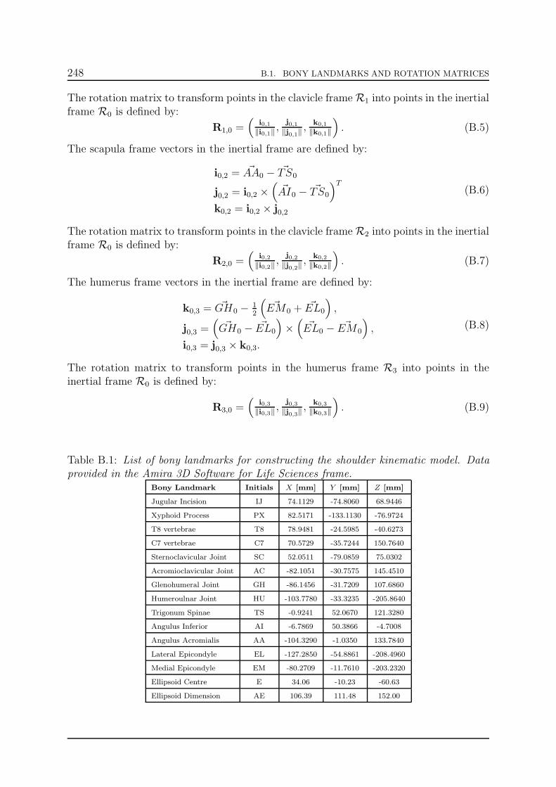
248 B.1. BONY LANDMARKS AND ROTATION MATRICES
The rotation matrix to transform points in the clavicle frameR1 into points in the inertialframe R0 is defined by:
R1,0 =(
i0,1‖i0,1‖
,j0,1
‖j0,1‖,
k0,1
‖k0,1‖
)
. (B.5)
The scapula frame vectors in the inertial frame are defined by:
i0,2 = ~AA0 − ~TS0
j0,2 = i0,2 ×(
~AI0 − ~TS0
)T
k0,2 = i0,2 × j0,2
(B.6)
The rotation matrix to transform points in the clavicle frameR2 into points in the inertialframe R0 is defined by:
R2,0 =(
i0,2‖i0,2‖
,j0,2
‖j0,2‖,
k0,2
‖k0,2‖
)
. (B.7)
The humerus frame vectors in the inertial frame are defined by:
k0,3 = ~GH0 − 12
(
~EM 0 + ~EL0
)
,
j0,3 =(
~GH0 − ~EL0
)
×(
~EL0 − ~EM 0
)
,
i0,3 = j0,3 × k0,3.
(B.8)
The rotation matrix to transform points in the humerus frame R3 into points in theinertial frame R0 is defined by:
R3,0 =(
i0,3‖i0,3‖
,j0,3
‖j0,3‖, k0,3
‖k0,3‖
)
. (B.9)
Table B.1: List of bony landmarks for constructing the shoulder kinematic model. Dataprovided in the Amira 3D Software for Life Sciences frame.
Bony Landmark Initials X [mm] Y [mm] Z [mm]
Jugular Incision IJ 74.1129 -74.8060 68.9446
Xyphoid Process PX 82.5171 -133.1130 -76.9724
T8 vertebrae T8 78.9481 -24.5985 -40.6273
C7 vertebrae C7 70.5729 -35.7244 150.7640
Sternoclavicular Joint SC 52.0511 -79.0859 75.0302
Acromioclavicular Joint AC -82.1051 -30.7575 145.4510
Glenohumeral Joint GH -86.1456 -31.7209 107.6860
Humeroulnar Joint HU -103.7780 -33.3235 -205.8640
Trigonum Spinae TS -0.9241 52.0670 121.3280
Angulus Inferior AI -6.7869 50.3866 -4.7008
Angulus Acromialis AA -104.3290 -1.0350 133.7840
Lateral Epicondyle EL -127.2850 -54.8861 -208.4960
Medial Epicondyle EM -80.2709 -11.7610 -203.2320
Ellipsoid Centre E 34.06 -10.23 -60.63
Ellipsoid Dimension AE 106.39 111.48 152.00

B.2. MASS, INTERTIA AND GLENDOID STABILITY 249
B.2 Mass, Intertia and Glendoid Stability
The dynamic model was constructed using the inertial data from [28] (Table B.2). Thecentre of gravity of each bone is defined by:
CG0,1 : ~x0,1 = ~SC0 +1
2R1,0
(
~AC1
)
, (B.10)
CG0,2 : ~x0,2 = ~SC0 +R1,0
(
~AC1
)
+1
3R2,0
(
~AI2
)
, (B.11)
CG0,3 : ~x0,3 = ~SC0 +R1,0
(
~AC1
)
+R2,0
(
~GH2
)
+R3,0
(
~HU2
)
. (B.12)
The humeral data is also the data for the outstretched arm.
Table B.2: List of inertial data to construct dynamic model. The data taken from [28].The humerus data includes the arm.
Data Type Clavicle Scapula Humerus (Arm)
Mass [kg] 0.156 0.704 3.67
Transverse Inertia [kgm2] 0.001 0.007 1.996
Longitudinal Inertia [kgm2] 0.003 0.007 0.309
The glenoid stability constraint is defined using the data collected from the MRI scans.The data contains the dimensions of the glenoid ellipse (Hy, Hz), the centre of the glenoidellipse GC in the inertial frame but with respect to the centre of the glenohumeral joint.The cone reference frame axes are defined by:
i0,5 = ~GH0 − ~GC0,k0,5 = (0, 0, 1)T ,j0,5 = k0,5 × i0,5,k0,5 = i0,5 × j0,5.
(B.13)
The rotation matrix to transform a point in the glenoid frame into a point in the inertialframe is defined by:
R5,0 =(
i0,5‖i0,5‖
,j0,5
‖j0,5‖, k0,5
‖k0,5‖
)
. (B.14)
Table B.3: The data is provided in the thorax/inertial reference system.Data Type X [mm] Y [mm] Z [mm]
Centre of Glenoid GC -13.80 -15.50 -2.46
Suprerior/Inferior Dimension Hz , [mm] 17.5
Posterior/Anterior Dimension Hy, [mm] 12.8

250 B.3. MUSCLE GEOMETRY AND WRAPPING
B.3 Muscle Geometry and Wrapping
This section provides the geometric data necessary to construct the muscle wrapping.The data contains the origin, the insertion and any via points of each muscle. Eachmuscle has been given a trio of anchor points to construct the third order splines of themuscle origins, insertions and via points. In the local bone frame, the spline constructionis defined by:
Pi,k(µ) : ~pi.k(µ) =
(µ3 µ2 µ 1
)S
~pi,s~pi,s~pi,m~pi,f
if 0 ≤ µ < 0.5
(µ3 µ2 µ 1
)S
~pi,s~pi,m~pi,f~pi,f
if 0.5 ≤ µ ≤ 1
,S =
−1
2
3
2−
3
2
1
2
1 5
22 −
1
2
−1
20 1
20
0 1 0 0
. (B.15)
where µ is the spline parameterisation variable. Each point is defined in terms of its x-,y-, and z-coordinates in the Amira frame. The bone reference frame Ri (i = 0, 1, 2, 3)to which the point is attached is also given.
The data contains the wrapping constraints, modelling the anatomical constraints ofthe real shoulder which are either other muscles or bony structures. The constraints areof the same type as the ones defined in [76]. The constraints are one of the following:
• None: The muscle has no wrapping constraints,
• Single: The muscle has single cylinder wrapping constraint,
• Double: The muscle has a double wrapping constraint,
• Stub: The muscle has a sphere capped cylinder wrapping constraint.
Each of the constraint types is a smooth surface. The surfaces are characterised bya point, an orientation and a dimension. The point fixes the location of the constraintsurface with respect to the bone which it represents. The point is designated by Oi,w. Thesubindex i is the index of the bone to which the constraint is attached. The orientation isparameterised by a single vector ~zi,w. The constraint surfaces are cylinders, the vector ~zi,wis the cylinder axes direction vector with respect to same bone as Oi,w. The dimension Dw
is the diameter of the cylinder. For sphere capped cylinders, the half sphere is situatedin the positive z-axis direction. All the data is provided in the MATLAB frame. Thewrappings are constructed using the geometric algorithms from [75]. The Dw values havea sign which indicates which path the muscle segment takes around the cylinder.

B.3. MUSCLE GEOMETRY AND WRAPPING 251
Table B.4: Muscle wrapping data for constructing the muscle geometric model. Data isprovided in the Amira 3D Software for Life Sciences frame.
Subclavius Origin R0 Insertion R1
Point Id X [mm] Y [mm] Z [mm] X [mm] Y [mm] Z [mm]
~pi,s 47.3022 -21.8898 21.4841 124.6826 -8.302 8.677
~pi,m 40.1071 -16.5496 14.6819 106.0602 -0.31249 6.6497
~pi,f 32.8671 -11.9641 8.885 89.4372 5.0201 2.5492
Type: None
Serratus Anterior Sup. Origin R0 Insertion R2
Point Id X [mm] Y [mm] Z [mm] X [mm] Y [mm] Z [mm]
~pi,s 94.7792 -28.9257 5.9179 -121.029 2.772 -7.7555
~pi,m 78.1183 -33.3803 35.5112 -119.0805 8.5437 6.9199
~pi,f 65.8219 -41.8242 48.2433 -113.547 21.9331 21.7063
Type: Single Centre R0 Axis R0
Radius: 62.4636 [mm] 78.9075 -68.7859 10.967 0.70426 0.099214 -0.70297
Serratus Anterior Mid. Origin R0 Insertion R2
Point Id X [mm] Y [mm] Z [mm] X [mm] Y [mm] Z [mm]
~pi,s 100.5324 -8.6176 -52.4343 -124.7227 0.035524 -48.6225
~pi,m 95.1886 -15.1122 -25.1971 -122.906 -0.065892 -32.328
~pi,f 92.3368 -19.8318 -4.0179 -121.6444 2.3897 -13.4542
Type: Single Centre R0 Axis R0
Radius: 83.3324 [mm] 90.9775 -58.6028 -37.1678 0.43024 0.096155 -0.89758
Serratus Anterior Inf. Origin R0 Insertion R2
Point Id X [mm] Y [mm] Z [mm] X [mm] Y [mm] Z [mm]
~pi,s 114.3886 -82.1116 -165.5598 -129.361 7.5023 -124.0556
~pi,m 126.4075 -24.6966 -110.3313 -131.0031 0.9116 -88.1316
~pi,f 104.6699 -7.7682 -54.275 -126.5523 0.86269 -55.1583
Type: Single Centre R0 Axis R0
Radius: 114.0104 [mm] 66.9717 -55.2411 -75.9889 -0.019976 -0.01175 -0.99973
Trapezius C1-C6 Origin R0 Insertion R1
Point Id X [mm] Y [mm] Z [mm] X [mm] Y [mm] Z [mm]
~pi,s 17.933 -40.1305 144.999 110.4728 2.4786 12.9065
~pi,m 6.9117 -54.655 130.1448 142.5331 -4.7352 13.0363
~pi,f 4.4143 -69.5781 116.992 157.5417 -5.5202 7.9516
Type: Single Centre R0 Axis R0
Radius: 65.23 [mm] 63.4174 -48.0171 130.8476 0.17043 -0.90071 0.39959
Trapezius C7 Origin R0 Insertion R2
Point Id X [mm] Y [mm] Z [mm] X [mm] Y [mm] Z [mm]
~pi,s 9.3247 -95.6367 80.1995 -45.7456 0.8996 13.1699
~pi,m 9.7249 -86.2045 101.2646 -28.0669 7.2086 14.5804
~pi,f 3.4617 -72.0971 113.1491 -13.8296 18.7389 12.4691
Type: Single Centre R0 Axis R0
Radius: 76.1526 [mm] 48.4107 -55.7942 80.0767 -0.11248 0.89622 0.42911

252 B.3. MUSCLE GEOMETRY AND WRAPPING
Trapezius T1 Origin R0 Insertion R2
Point Id X [mm] Y [mm] Z [mm] X [mm] Y [mm] Z [mm]
~pi,s 9.5704 -111.3463 35.6335 -79.9134 -11.4331 7.743
~pi,m 7.7586 -106.525 56.8341 -62.1015 -6.056 11.0343
~pi,f 5.5539 -97.0621 78.3253 -50.1784 -0.97814 13.5338
Type: Single Centre R0 Axis R0
Radius: 95.6832 [mm] 63.7866 -84.4989 52.4261 -0.025594 0.53043 0.84734
Trapezius T2-T7 Origin R0 Insertion R2
Point Id X [mm] Y [mm] Z [mm] X [mm] Y [mm] Z [mm]
~pi,s 4.3375 -114.3685 -203.4799 -86.013 -12.1708 6.5964
~pi,m 6.1887 -125.1353 -91.0941 -95.9787 -8.495 -2.1346
~pi,f 7.4436 -117.4578 32.2477 -113.4155 -3.393 -0.42729
Type: Single Centre R0 Axis R0
Radius: 121.5968 [mm] 50.3929 -74.9743 -70.7722 0.012283 0.012307 0.99985
Levator Scapulae Origin R0 Insertion R2
Point Id X [mm] Y [mm] Z [mm] X [mm] Y [mm] Z [mm]
~pi,s 16.0717 -42.3965 166.4632 -112.9184 17.2979 23.1744
~pi,m 15.824 -50.0719 154.5936 -117.6254 10.792 15.6349
~pi,f 16.8122 -56.7843 141.4639 -117.2106 4.8568 8.3213
Type: None
Rhomboid Minor Origin R0 Insertion R2
Point Id X [mm] Y [mm] Z [mm] X [mm] Y [mm] Z [mm]
~pi,s 10.1598 -85.1539 101.1227 -119.332 7.178 7.618
~pi,m 9.7589 -91.293 90.9366 -119.7223 0.62991 -2.048
~pi,f 9.6095 -96.2044 79.1984 -121.3933 -0.48993 -11.5158
Type: None
Rhomboid Major T1-T2 Origin R0 Insertion R2
Point Id X [mm] Y [mm] Z [mm] X [mm] Y [mm] Z [mm]
~pi,s 7.7951 -100.6494 72.6624 -122.0314 -1.3421 -16.8202
~pi,m 12.0043 -108.3404 54.4455 -124.3712 -2.7343 -38.3552
~pi,f 13.2638 -114.3854 32.1064 -127.6047 -1.1541 -65.5843
Type: Single Centre R0 Axis R0
Radius: 90.2222 [mm] 49.2891 -79.2561 39.7921 -0.077561 0.21154 0.97429
Rhomboid Major T3-T4 Origin R0 Insertion R2
Point Id X [mm] Y [mm] Z [mm] X [mm] Y [mm] Z [mm]
~pi,s 16.0253 -120.6784 -20.5786 -132.9776 2.8646 -122.1601
~pi,m 14.735 -119.6945 5.0805 -132.0646 -0.99899 -94.523
~pi,f 13.6637 -117.1852 25.4825 -129.3213 -1.4088 -70.663
Type: Single Centre R0 Axis R0
Radius: 90.2222 [mm] 52.2229 -88.3502 -9.6992 -0.052258 0.054114 0.99717

B.3. MUSCLE GEOMETRY AND WRAPPING 253
Pectoralis Minor Origin R0 Insertion R2
Point Id X [mm] Y [mm] Z [mm] X [mm] Y [mm] Z [mm]
~pi,s 112.4553 1.9047 -114.5028 -33.6689 66.8144 -12.1784
~pi,m 108.3519 -2.7766 -85.7049 -36.7303 63.7507 -9.9863
~pi,f 104.19 -11.663 -48.3304 -40.1253 60.8655 -7.3816
Type: None
Pectoralis Major Sup. Origin R1 Insertion R3
Point Id X [mm] Y [mm] Z [mm] X [mm] Y [mm] Z [mm]
~pi,s 6.5281 6.8431 -6.0261 6.0428 10.2123 -81.5794
~pi,m 30.0086 13.1245 -4.589 5.0411 9.4042 -89.0349
~pi,f 53.5354 17.2967 -3.6244 3.8217 8.5626 -94.5638
Type: Single Centre R0 Axis R0
Radius: 78.733 [mm] 89.7779 -32.6979 -17.2779 -0.31284 0.31596 -0.89571
Pectoralis Major Mid. Origin R0 Insertion R3
Point Id X [mm] Y [mm] Z [mm] X [mm] Y [mm] Z [mm]
~pi,s 8.527 24.306 -78.8645 6.7832 10.2222 -68.0628
~pi,m 9.7158 16.0647 -50.3474 5.727 10.3971 -75.4138
~pi,f 24.1675 -2.6064 -12.786 5.7225 10.2745 -83.3312
Type: Single Centre R0 Axis R0
Radius: 103.5784 [mm] 72.1919 -31.2906 -52.9492 -0.0025661 0.32076 -0.94716
Pectoralis Major Inf. Origin R0 Insertion R3
Point Id X [mm] Y [mm] Z [mm] X [mm] Y [mm] Z [mm]
~pi,s 45.934 39.1666 -157.381 7.5278 12.1484 -52.3811
~pi,m 10.9816 34.5373 -117.0259 7.0048 11.1011 -62.0383
~pi,f 8.7838 25.2681 -85.1756 6.6532 10.5044 -70.9866
Type: Single Centre R0 Axis R0
Radius: 119.8136 [mm] 65.2042 -25.25 -103.5016 0.36618 0.15146 -0.91814
Latisimuss Dorsi Thoracic Origin R0 Insertion R3
Point Id X [mm] Y [mm] Z [mm] X [mm] Y [mm] Z [mm]
~pi,s 10.6486 -127.1927 -59.9564 6.2547 10.1442 -81.9018
~pi,m 8.025 -125.1166 -121.7227 6.1941 10.4861 -77.1875
~pi,f 5.3463 -122.0054 -173.2486 5.6998 10.404 -70.9403
Type: Double Centre R0 Axis R0
Radius: 126.8796 [mm] 66.287 -75.6991 -117.425 0.064623 -0.03431 0.99732
Centre R3 Axis R3
Radius: 27.2296 [mm] -5.1088 -2.0566 -75.6967 0.019975 0.067257 -0.99754
Latisimuss Dorsi Lumbar Origin R0 Insertion R3
Point Id X [mm] Y [mm] Z [mm] X [mm] Y [mm] Z [mm]
~pi,s 16.6142 -92.133 -303.7379 7.1407 11.6001 -56.8227
~pi,m 12.0451 -107.6165 -240.7004 6.2475 11.0229 -62.8968
~pi,f 5.1454 -121.5951 -186.0512 5.6569 10.0836 -68.0006
Type: Double Centre R0 Axis R0
Radius: 144.3066 [mm] 78.1611 -42.8298 -240.6841 -0.075133 -0.11952 0.98999
Centre R3 Axis R3
Radius: 27.2296 [mm] -6.9135 -2.3851 -63.8543 0.1204 -0.0078034 -0.99269

254 B.3. MUSCLE GEOMETRY AND WRAPPING
Latisimuss Dorsi Iliac Origin R0 Insertion R3
Point Id X [mm] Y [mm] Z [mm] X [mm] Y [mm] Z [mm]
~pi,s 29.3382 -114.9391 -371.6228 7.2496 10.6415 -43.4864
~pi,m 21.7063 -96.3715 -338.6665 6.9115 10.7837 -49.0554
~pi,f 17.3063 -89.5 -308.8827 7.2819 11.9251 -53.6699
Type: Double Centre R0 Axis R0
Radius: 168.1542 [mm] 78.0742 -36.8231 -202.3643 -0.14768 -0.10953 0.98295
Centre R3 Axis R3
Radius: 27.2296 [mm] -5.7337 1.1047 -52.4145 0.038747 -0.11434 -0.99269
Anterior Deltoid Origin R1 Insertion R3
Point Id X [mm] Y [mm] Z [mm] X [mm] Y [mm] Z [mm]
~pi,s 126.6803 -0.87531 10.275 9.4509 4.0979 -129.2376
~pi,m 143.604 -0.39192 7.1363 9.56 5.2246 -139.2259
~pi,f 160.8002 6.0558 0.40596 9.3273 5.3664 -148.3023
Point Id Via A Via B R3
~pi,s 23.0056 13.9745 -102.6272
~pi,m 23.4855 10.2534 -102.7768
~pi,f 23.3426 5.9889 -102.9171
Type: Single Centre R2 Axis R2
Radius: -73.1998 [mm] -14.6895 44.6045 -32.5017 0.73986 -0.50467 0.44489
Middle Deltoid Origin R2 Insertion R3
Point Id X [mm] Y [mm] Z [mm] X [mm] Y [mm] Z [mm]
~pi,s -0.20406 -0.074248 0.13482 10.2435 -0.36749 -129.4244
~pi,m 11.8236 27.4926 1.9362 10.8922 0.59153 -139.4917
~pi,f 1.0065 39.9286 9.0799 10.3543 1.1799 -147.7047
Point Id Via A R2 Via B R3
~pi,s 20.1262 5.4089 -0.075243 21.9272 -7.8303 -103.3292
~pi,m 19.672 32.11 0.066403 22.6176 -3.6131 -103.215
~pi,f 8.8135 52.8413 2.7152 23.3555 1.4133 -103.0751
Type: Stub Centre R3 Axis R3
Radius: 55.3988 [mm] 6.9099 -3.21 0.56374 0.28815 -0.024237 0.95728
Posterior Deltoid Origin R2 Insertion R3
Point Id X [mm] Y [mm] Z [mm] X [mm] Y [mm] Z [mm]
~pi,s -69.6536 -10.1689 2.1174 9.7675 -4.5744 -129.1426
~pi,m -29.2521 -3.4775 7.3322 11.1254 -3.3937 -138.7676
~pi,f -3.5772 -0.92811 -0.30127 10.6649 -3.3442 -147.7837
Point Id Via A R2 Via B R3
~pi,s -38.2118 -13.8338 -13.9952 14.3382 -20.1916 -103.4148
~pi,m -14.3091 -11.162 -6.1601 18.0168 -16.2487 -103.4438
~pi,f 9.0994 -1.4206 -8.9833 20.6761 -11.6495 -103.4046
Type: Stub Centre R2 Axis R2
Radius: 58.0972 [mm] 3.4356 31.7188 -25.3069 0.2912 -0.17793 0.93997

B.3. MUSCLE GEOMETRY AND WRAPPING 255
Supraspinatus Origin R2 Insertion R3
Point Id X [mm] Y [mm] Z [mm] X [mm] Y [mm] Z [mm]
~pi,s -92.7644 31.4612 22.0077 23.834 9.767 6.4975
~pi,m -101.1358 22.9552 13.4189 25.7241 2.5645 5.9216
~pi,f -104.8622 10.9751 5.223 24.4828 -5.4397 3.8368
Point Id Via A R2 Via B
~pi,s -54.4191 40.7818 5.6817
~pi,m -56.2815 27.0486 4.2737
~pi,f -58.7211 13.4467 -2.6139
Type: Single Centre R3 Axis R3
Radius: 41.9158 [mm] 1.167 2.3044 2.4789 0.0013802 0.99991 0.013388
Infraspinatus Origin R2 Insertion R3
Point Id X [mm] Y [mm] Z [mm] X [mm] Y [mm] Z [mm]
~pi,s -124.0628 -1.9184 -105.6435 9.8596 -17.645 -7.6911
~pi,m -115.8308 -3.1223 -58.2159 17.373 -16.6175 0.37414
~pi,f -107.9192 0.17217 -13.055 23.5991 -10.3027 3.044
Point Id Via A R2 Via B
~pi,s -38.4143 9.8302 -57.7836
~pi,m -38.6937 3.2995 -30.2236
~pi,f -35.5198 3.7126 -3.7866
Type: Stub Centre R3 Axis R3
Radius: 41.9158 [mm] 1.0394 -0.96844 1.8502 -0.0013809 -0.99991 -0.013387
Subscapularis Origin R2 Insertion R3
Point Id X [mm] Y [mm] Z [mm] X [mm] Y [mm] Z [mm]
~pi,s -123.4762 7.3923 -122.5987 -3.3505 20.0523 -13.5801
~pi,m -116.0687 1.189 -29.0969 -4.1732 23.0766 -6.468
~pi,f -103.6795 22.1996 7.8449 -0.21938 24.4173 -0.067492
Point Id Via A R2 Via B
~pi,s -66.6935 26.507 -53.8117
~pi,m -65.0629 28.4745 -31.1974
~pi,f -66.4803 35.0349 -13.4779
Type: Stub Centre R3 Axis R3
Radius: 41.9158 [mm] -19.6158 0.39544 -5.8439 0.0013825 0.99991 0.013387
Teres Minor Origin R2 Insertion R3
Point Id X [mm] Y [mm] Z [mm] X [mm] Y [mm] Z [mm]
~pi,s -87.0304 2.9277 -98.9601 9.5286 -8.4224 -24.7259
~pi,m -69.9267 6.3263 -71.0541 8.6471 -11.0262 -17.2425
~pi,f -53.4579 11.6022 -54.0939 9.0415 -15.3647 -11.0582
Point Id Via A R2 Via B
~pi,s -39.943 3.277 -82.3658
~pi,m -33.9335 3.9595 -69.5523
~pi,f -32.2664 3.7599 -57.2188
Type: Stub Centre R3 Axis R3
Radius: 41.9158 [mm] -12.696 -1.8977 -28.0528 -0.0013809 -0.99991 -0.013387
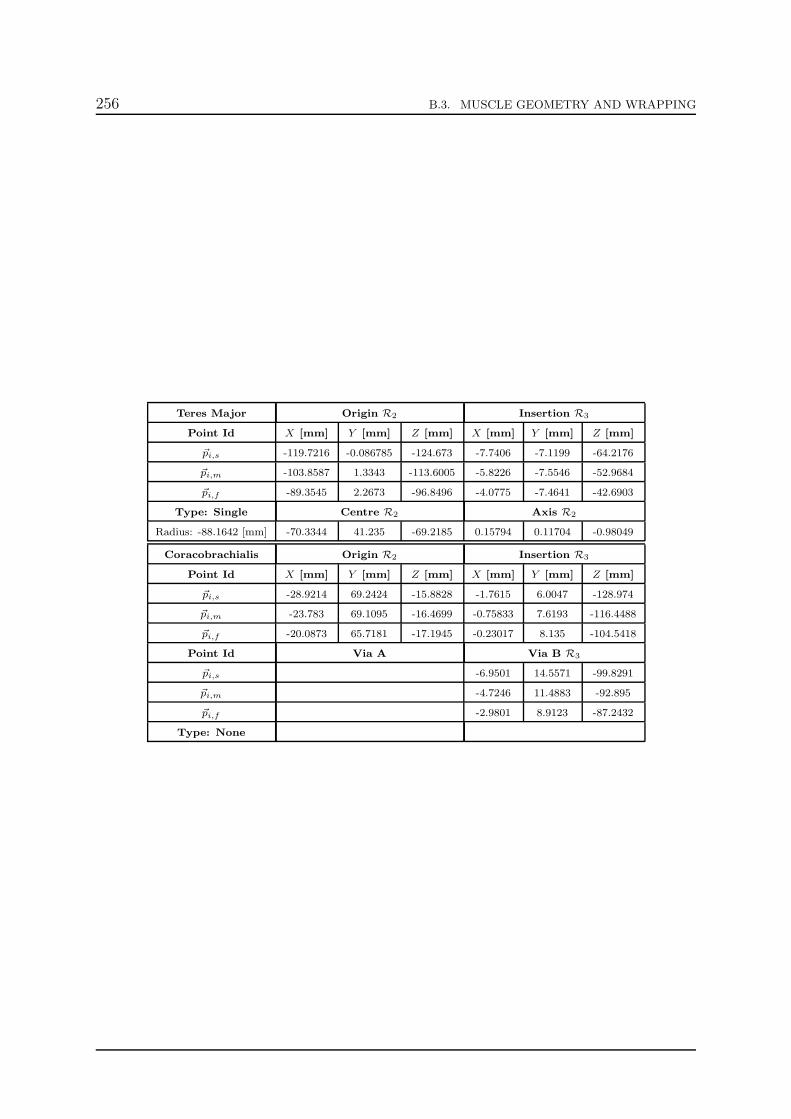
256 B.3. MUSCLE GEOMETRY AND WRAPPING
Teres Major Origin R2 Insertion R3
Point Id X [mm] Y [mm] Z [mm] X [mm] Y [mm] Z [mm]
~pi,s -119.7216 -0.086785 -124.673 -7.7406 -7.1199 -64.2176
~pi,m -103.8587 1.3343 -113.6005 -5.8226 -7.5546 -52.9684
~pi,f -89.3545 2.2673 -96.8496 -4.0775 -7.4641 -42.6903
Type: Single Centre R2 Axis R2
Radius: -88.1642 [mm] -70.3344 41.235 -69.2185 0.15794 0.11704 -0.98049
Coracobrachialis Origin R2 Insertion R3
Point Id X [mm] Y [mm] Z [mm] X [mm] Y [mm] Z [mm]
~pi,s -28.9214 69.2424 -15.8828 -1.7615 6.0047 -128.974
~pi,m -23.783 69.1095 -16.4699 -0.75833 7.6193 -116.4488
~pi,f -20.0873 65.7181 -17.1945 -0.23017 8.135 -104.5418
Point Id Via A Via B R3
~pi,s -6.9501 14.5571 -99.8291
~pi,m -4.7246 11.4883 -92.895
~pi,f -2.9801 8.9123 -87.2432
Type: None
Bibliography
[1] J. Ackermann. Der Entwurf Regelungssyteme im Zustandsraum. Regelungstechnikund Prozessedatenverarbeitung, 7:297–300, 1972.
[2] D.C. Ackland, P. Pak, M. Richardson, and M.G. Pandy. Moment arms of themuscles crossing the anatomical shoulder. Journal of Anatomy, 213(4):383–390,2008.
[3] M. Aeberhard, Y. Michellod, P. Mullhaupt, A. Terrier, D.P. Pioletti, and D. Gillet.Dynamical biomechanical model of the shoulder: Null space based optimization ofthe overactuated system. In Robotics and Biomimetics, 2008. ROBIO 2008. IEEEInternational Conference on, pages 67 –73, feb. 2009.
[4] F. Altpeter. Friction Modeling, Identification and Compensation. PhD thesis,EPFL, Lausanne, 1999.
[5] K.N. An, Y. Ueba, E.Y. Chao, W.P. Cooney, and R.L. Linscheid. Tendon excursionand moment arm of index finger muscles. Journal of Biomechanics, 16(6):419 – 425,1983.
[6] K.N. An, B.M. Kwak, E.Y. Chao, and B.F. Morrey. Determination of muscleand joint forces: a new technique to solve the indeterminate problem. Journal ofBiomechanical Engineering, 106:364–367, 1984.
[7] K.N. An, K. Takahashi, T.P. Harrigan, and E.Y. Chao. Determination of muscleorientations and moment arms. Journal of Biomechanical Engineering, 106(3):280–282, 1984.
[8] M.S. Andersen, M. Damsgaard, and J. Rasmussen. Kinematic analysis of over-determinate biomechanical systems. Computer Methods in Biomechanics andBiomedical Engineering, 12(4):371–384, 2009.
[9] M.S. Andersen, M. Damsgaard, and J. Rasmussen. Force-dependent kinematics: anew analysis method for non-conforming joints. In XIII International Symposiumon Computer Simulation in Biomechanics, 2011.
[10] M. Apreleva, I.M. IV Parsons, J.P. Warner, F.H. Fu, and S.L.-Y. Woo. Exper-imental investigation of reaction forces at the glenohumeral joint during activeabduction. Journal of Shoulder and Elbow Surgery, 9(5):409 – 417, 2000.
257

258 BIBLIOGRAPHY
[11] Xueling Bai, Gaofeng Wei, Ming Ye, Dongmei Wang, Yan Hu, Zongliang Liu, Wen-zhong Nie, Linlin Zhang, Wenting Ji, Yunting Li, and Chengtao Wang. Finiteelement musculoskeletal modeling of mechanical virtual human of china. In Bioin-formatics and Biomedical Engineering, 2008. ICBBE 2008. The 2nd InternationalConference on, pages 1847–1850, May 2008.
[12] Sir R.S. Ball. Theory of Screws: a study in the dynamics of a rigid body. HodgesPublication, Dublin, 1876.
[13] J.W. Baumgarte. A new method of stabilization for holonomic constraints. Journalof Applied Mechanics, 50:869–870, 1983.
[14] M.S. Bazaraa, H.D. Sherali, and Shetty C. M. Nonlinear Programming: Theoryand Algorithms. John Wiley and Sons, New York, 2 edition, 1993.
[15] M.F. Bear, B.W. Connors, and M.A. Paradiso. Neuroscience: Exploring the brain.Lippincott, Williams & Wilkins, 3rd edition, 2000.
[16] R. Becker, A. Berth, M. Nehring, and F. Awiszus. Neuromuscular quadricepsdysfunction prior to osteoarthritis of the knee. Journal of Orthopaedic Research,22(4):768–773, 2004.
[17] G. Bergmann, F. Graichen, A. Bender, A. Rohlmann, A. Halder, A. Beier, andP. Westerhoff. In vivo gleno-humeral joint loads during forward flexion and abduc-tion. Journal of Biomechanics, 44(8):1543 – 1552, 2011.
[18] J.M. Berthelot. Mechanics of Rigid Bodies. Springer, New-York, 1999.
[19] D. Blana and E.K. Kirsch R.F. Chadwick. Combined feedforward and feedbackcontrol of a redundant, nonlinear, dynamic musculoskeletal system. Med. Biol.Eng. Comput., 47:533–542, 2009.
[20] B. Bolsterlee, H.E. Veeger, and F.C.T. van der Helm. Modelling clavicular andscapular kinematics: from measurement to simulation. Medical & Biological Engi-neering & Computing, 52(3):283–291, 2014.
[21] P. Bosscher, A.T. Riechel, and I. Ebert-Uphoff. Wrench-feasible workspace gen-eration for cable-driven robots. Robotics, IEEE Transactions on, 22(5):890–902,2006.
[22] J. Botsis and M. Deville. Mecanique des Milieux Continus: Une Introduction.Lausanne: Presses Polytechniques et Universitaires Romandes, 2006.
[23] O. Bottema and Roth B. Theoretical Kinematics. Dover Publications, 2012.
[24] S. Boyd and L. Vandenberghe. Convex Optimization. Cambridge University Press,2004.
[25] P.W. Brand, Cranor K.C., and J.C. Ellis. Tendon and pulleys at the metacarpopha-langeal joint of a finger. The Journal of Bone & Joint Surgery, 57(6):779–784, 1975.

BIBLIOGRAPHY 259
[26] R.A. Brand, D.R. Pedersen, and J.A. Friederich. The sensitivity of muscle forcepredictions to changes in physiologic cross-sectional area. Journal of Biomechanics,19:589–596, 1986.
[27] K.D. Brandt, P. Dieppe, and E.L. Randin. Etiopathogenesis of osteoarthritis. Jour-nal of the American Osteopathic Association, 34:531–559, 2008.
[28] M.D.K. Breteler, C.W. Spoor, and F.C.T. van der Helm. Measuring muscle andjoint geometry parameters of a shoulder for modeling purposes. Journal of Biome-chanics, 32(11):1191 – 1197, 1999.
[29] T. Bruckmann and A. Pott. Cable-driven parallel robots. Springer Science & Busi-ness Media, 2013.
[30] J.A. Buckwalter, W.D. Stanish, R.N. Rosier, R.C. Schenck, D.A. Dennis, and R.D.Coutts. The increasing need for nonoperative treatment of patients with osteoarthri-tis. Clinical Orthopaedics and Related Research, 385:36–45, 2001.
[31] J. Burdick. Kinematic analysis and design of redundant robot manipulators. PhDthesis, Standford University, Standford, 1988.
[32] R. Cailliet. The Illustrated Guide to Functional Anatomy of the MusculokeletalSystem. American Medical Association, 2004.
[33] S. Carbes. Shoulder rhythm report: Anyscript support wiki, 2011.
[34] B. Chachuat, B. Srinivasan, and D. Bonvin. Adaptation strategies for real-timeoptimization. Computers & Chemical Engineering, 33:1557–1567, 2009.
[35] B.C. Chachuat. Nonlinear and dynamic optimisation, from theory to practice, 2006.
[36] E.K.J. Chadwick and F.C.T. van der Helm. Musculoskeletal modelling of the shoul-der, 2003.
[37] I.W. Charlton and G.R. Johnson. A model for the prediction of the forces at theglenohumeral joint. In Proc. Inst. Mech. Eng. [H], volume 220, page 801–812, 2006.
[38] W.I. Charlton and G.R Johnson. Application of spherical and cylindrical wrappingalgorithms in a musculoskeletal model of the upper limb. Journal of Biomechanics,34(9):1209 – 1216, 2001.
[39] M. Chasles. Note sur les proprietes generales du systeme de deux corps semblablesentr’eux et places d’une maniere quelconque dans l’espace; et sur le deplacement finiou infiniment petit d’un corps solide libre. Bulletin des Sciences Mathematiques,Astronomiques, Physiques et Chimiques, 14:321–326, 1830.
[40] C.-T. Chen. Linear System Theory and Design. Oxford University Press, New YorkOxford, 3 edition, 1999.
[41] W. Chen and E. De Schutter. Python-based geometry preparation and simulationvisualization toolkits for steps. Frontiers in Neuroinformatics, 2014.

260 BIBLIOGRAPHY
[42] L. Cheze, B.J. Fregly, and J. Dimnet. A solidification procedure to facilitate kine-matic analyses based on video system data. Journal of Biomechanics, 28(7):879 –884, 1995.
[43] E.A. Codman. The Shoulder: Rupture of the Supraspinatus Tendon and OtherLesions In or About the Subacromial Bursa. Boston: Thomas Todd Co., 1934.
[44] E. Conkur and R. Buckingham. Clarifying the definition of redundancy as used inrobotics. Robotica, 15:583 – 586, 1997.
[45] A.R. Crossman and D. Neary. Neuroanatomy, An illustrated colour text. ChuchillLivingstone Elsevier, 4rd edition, 2010.
[46] A. Curnier. Mecanique des Solides Deformables. Lausanne: Presses Polytechniqueset Universitaires Romandes, 2005.
[47] A.G. Cutti and E.K. Chadwick. Shoulder biomechanics and the success of transla-tional research. Medical & Biological Engineering & Computing, 52:205–210, 2014.
[48] A.G. Cutti and H.E.J. (DirkJan) Veeger. Shoulder biomechanics: today’s consensusand tomorrow’s perspectives. Medical & Biological Engineering & Computing, 47:463–466, 2009.
[49] M. Damsgaard, J. Rasmussen, S.T. Christensen, E. Surma, and M. de Zee. Analysisof musculoskeletal systems in the anybody modeling system. Simulation ModellingPractice and Theory, 14(8):1100 – 1111, 2006.
[50] J. H. deGroot and R. Brand. A three-dimension regression model of the shoulderrhythm. Clinical biomechanics, 16:735–743, 2001.
[51] S.L. Delp and J.P. Loan. A graphics-based software system to develop and analyzemodels of musculoskeletal structures. Computers in Biology and Medicine, 25(1):21 – 34, 1995.
[52] S.L. Delp, F.C. Anderson, A.S. Arnold, P. Loan, A. Habib, C.T. John, E. Guen-delman, and D.G. Thelen. Opensim: Open-source software to create and analysedynamic simulations of movement. IEEE Transactions on Biomedical Engineering,54(11):1940–1950, 2007.
[53] W. T. Dempster. Mechanism of shoulder movement. Archives of Physical Medicineand Rehabilitation, 46(1):49–69, 1965.
[54] C.R. Dickerson, D.B. Chaffin, and R.E. Hughes. A mathematical musculoskeletalshoulder model for proactive ergonomic analysis. Computer Methods in Biome-chanics and Biomedical Engineering, 10:389–400, 2007.
[55] B.F. Dulin and C.F. Martin. Introduction to differential geometry for engineers.New York: Marcel Dekker, 1990.
[56] R. Dumas and L. Cheze. Soft tissue artifact compensation by linear 3d interpolationand approximation methods. Journal of Biomechanics, 42(13):2214 – 2217, 2009.

BIBLIOGRAPHY 261
[57] I. Ebert-Uphoff and P.A. Voglewede. On the connections between cable-drivenrobots, parallel manipulators and grasping. In Robotics and Automation, 2004.Proceedings. ICRA ’04. 2004 IEEE International Conference on, volume 5, pages4521–4526, April 2004.
[58] A. El Habachi, S. Duprey, L. Cheze, and R. Dumas. A parallel mechanism of theshoulder—application to multi-body optimisation. Multibody System Dynamics,pages 1–13, 2014.
[59] C. Engelhardt, D. Ingram, P. Muellhaupt, E. Pralong, A. Farron, D. Pioletti, andA. Terrier. Solving overconstrained kinematic in numerical shoulder model usingnullspace optimization. In 10th International Symposium on Computer Methods inBiomechanics and Biomedical Engineering, CMBBE 2012 Berlin, april 2012.
[60] Ch. Engelhardt, V.M. Camine, D. Ingram, Ph. Mullhaupt, A. Farron, D. Pioletti,and A. Terrier. Comparison of an emg-based and a stress-based method to pre-dict shoulder muscle forces. Computer Methods in Biomechanics and BiomedicalEngineering, 0(0):1–8, 2014.
[61] A. E. Engin and S. M. Chen. Statistical data base for the biomechanical propertiesof the human shoulder complex-part i : Kinematics of the shoulder complex. Journalof biomechanical engineering, 108:215–221, 1986.
[62] A. E. Engin and S. M. Chen. Statistical data base for the biomechanical propertiesof the human shoulder complex-part ii : Passive resistive properties beyond theshoulder complex sinus. Journal of biomechanical engineering, 108:222–227, 1986.
[63] A. E. Engin and S. T. Tumer. Three-dimensional kinematic modeling of the humanshoulder complex–part i: Physical model and determination of joint sinus cones.Journal of biomechanical engineering, 111(2):107–112, 1989.
[64] A. E. Engin and S. T. Tumer. Three-dimensional kinematic modeling of the humanshoulder complex–part ii: Mathematical modeling and solution via optimization.Journal of biomechanical engineering, 111(2):113–221, 1989.
[65] A.E. Engin. On the biomechanics of the shoulder complex. Journal of Biomechan-ics, 13(7):575 – 590, 1980.
[66] A. Erdemir, S. McLean, W. Herzog, and A.J. van den Bogert. Model-based es-timation of muscle forces exerted during movements. Clinical Biomechanics, 22:131–154, 2007.
[67] L. Euler. Quacunque corporum rigidorum. Novi Commentarii academiae scien-tiarum Petropolitanae, 20:189–207, 1776.
[68] P. Favre, J.G. Snedeker, and C. Gerber. Numerical modelling of the shoulder forclinical applications. Philosophical transactions. Series A, Mathematical, physical,and engineering sciences, 367:2095–2118., 2009.

262 BIBLIOGRAPHY
[69] Ph. Favre. A model to study active shoulder motion and stability. PhD thesis,ETHZ, Zurich, 2011.
[70] Ph. Favre, R. Sheikh, S.F. Fucentese, and H.A.C. Jacob. An algorithm for estima-tion of shoulder muscle forces for clinical use. Clinical Biomechanics, 20(8):822 –833, 2005.
[71] Ph. Favre, M. Senteler, J. Hipp, S. Scherrer, C. Gerber, and J.G. Snedeker. Anintegrated model of active glenohumeral stability. Journal of Biomechanics, 45(13):2248 – 2255, 2012.
[72] R.C. Fitzpatrick, J.L. Taylor, and D.I. McCloskey. Ankle stiffness of standinghumans in response to imperceptible perturbation: reflex and task-dependent com-ponents. Journal of Physiology, 454:533–547, 1992.
[73] L.D. Freedman and R.R. Munro. Abduction of the arm in the scapular plane:Scapular and glenohumeral movements. a roentgenographic study. The Journal ofBone & Joint Surgery, 48(8):1503–1510, 1966.
[74] B.A. Garner and M.G. Pandy. Musculoskeletal model of the upper limb based on thevisible human male dataset. Computer Methods in Biomechanics and BiomedicalEngineering, 4(2):107–124, 1999.
[75] B.A. Garner and M.G. Pandy. The obstacle-set method for representing musclepaths in musculoskeletal models. Computer Methods in Biomechanics and Biomed-ical Engineering, 3(1):1–30, 2000.
[76] B.A. Garner and M.G. Pandy. A kinematic model of the upper limb based on thevisible human project (vhp) image dataset. Computer Methods in Biomechanicsand Biomedical Engineering, 2(2):93–126, 2001.
[77] B.A. Garner and M.G. Pandy. Estimation of musculotendon properties in thehuman upper limb. Annals of Biomedical Engineering, 31:207–220, 2003.
[78] A. Goodwin, B.-H. Zhou, R.V. Baratta, M. Solomonow, and A. P. Keegan. Theinfluence of antagonist muscle control strategies on the isometric frequency responseof the cat’s ankle joint. Biomedical Engineering, IEEE Transactions on, 44(7):634–639, 1997.
[79] V.E. Gough and S.G. Whitehall. Universal tyre test machine. In Proceedings of9th. Int. Congress of F.I.S.I.T.A, 117, page 117–135, 1962.
[80] M. Gouttefarde and C.M. Gosselin. Analysis of the wrench-closure workspace ofplanar parallel cable-driven mechanisms. Robotics, IEEE Transactions on, 22(3):434–445, 2006.
[81] M. Gouttefarde, J.-P. Merlet, and D. Daney. Wrench-feasible workspace of parallelcable-driven mechanisms. In Robotics and Automation, 2007 IEEE InternationalConference on, pages 1492–1497, 2007.

BIBLIOGRAPHY 263
[82] H. Graichen, T. Stammberger, H. Bonel, K.-H. Englmeier, M. Reiser, and F. Eck-stein. Glenohumeral translation during active and passive elevation of the shoulder* a 3d open-mri study. Journal of Biomechanics, 33:609–613, 2000.
[83] H. Gray. Anatomy of the Human Body Gray. Philadelphia: Lea & Febiger, 1918.
[84] T.-J. Grewal. Quantifying the Shoulder Rhythm and Comparing Non-Invasive Meth-ods of Scapular Tracking for Overhead and Axially Rotated Humeral Postures. PhDthesis, University of Waterloo, Waterloo, 2011.
[85] M.J. Grey. Proprioceptive Sensory Feedback, Encyclopedia of Life Sciences. JohnWiley & Sons, 2010.
[86] C. Gruber and W. Benoit. Mechanique Generale. Lausanne: Presses Polytechniqueset Universitaires Romandes, 1998.
[87] B. Grunbaum. Convex Polytopes. Spinrger-Verlag, New York, 2 edition, 2003.
[88] S. Gupta, F.C.T. van der Helm, J.C. Sterk, F. van Keulen, and B.L. Kaptein. De-velopment and experimental validation of a three-dimensional finite element modelof the human scapula. Proc. Inst Mech Eng H., 218(2):127–142, 2004.
[89] L.N. Hand and J.D. Finch. Analytical Mechanics. Cambridge University Press,New York, 1998.
[90] R. Happee. Inverse dynamic optimization including muscular dynamics, a newsimulation method applied to goal directed movements. Journal of Biomechanics,27(5):953 – 960, 1994.
[91] R.S. Hartenberg and J. Denavit. Kinematic synthesis of linkages. New York:McGraw-Hill, 1964.
[92] M. Hassan and A. Khajepour. Optimization of actuator forces in cable-based par-allel manipulators using convex analysis. Robotics, IEEE Transactions on, 24(3):736–740, 2008.
[93] J. Hawkins. On Intelligence. Times Books, 2004.
[94] W. Herzog and P. Binding. Predictions of antagonistic muscular activity usingnonlinear optimization. Mathematical Biosciences, 111(2):217 – 229, 1992.
[95] A.V. Hill. The heat of shortening and the dynamic constants of muscle. Proceedingsof the Royal Society of London. Series B, Biological Sciences, 126(843):pp. 136–195,1938.
[96] K. Hoffman and R. Kunze. Linear Algebra. PHI Learning Private Limited, NewDelhi, 2 edition, 2010.
[97] N. Hogan. Adaptive control of mechanical impedance by coactivation of antagonisticmuscles. IEEE Transactions on Automatic Control, 29(8):681–690, 1984.

264 BIBLIOGRAPHY
[98] N. Hogan. The mechanics of multi-joint posture and movement control. BiologicalCybernetics, 52(5):315–331, 1985.
[99] D. Holm. Geometric mechanics, part i: Dynamics and symmetry. Imperial Collegecourse material, 2012.
[100] D. Holm. Geometric mechanics, part ii: Rotating, translating and rolling. ImperialCollege course material, 2012.
[101] K. R. S. Holzbaur, W. M. Murray, and S. L. Delp. A model of the upper extremityfor simulating musculoskeletal surgery and analyzing neuromuscular control. Annalsof Biomedical Engineering, 33:829–840, 2005.
[102] R.E. Hughes, G. Niebur, J. Liu, and K.N. An. Comparison of two methods forcomputing abduction moment arms of the rotator cuff. Journal of Biomechanics,31(2):157 – 160, 1998.
[103] C. Hogfors, B. Peterson, and P. Herberts. Biomechanical model of the humanshoulder-i. elements. Journal of biomechanics, 20(2):157–166, 1987.
[104] C. Hogfors, B. Peterson, G. Sigholm, and P. Herberts. Biomechanical model of thehuman shoulder-ii. the shoulder ryrthm. Journal of biomechanics, 24(8):699–709,1991.
[105] V.T. Inman, M. Saunders, and L.C. and Abbott. The role of the scapula in athleticshoulder function. 1944. Clinical Orthopaedics Related Research, 330:3–12, 1996.
[106] Abhinandan Jain. Minimal coordinates formulation of contact dynamics. In inMultibody Dynamics 2013, ECCOMAS Thematic Conference, pages 153–160, 2013.
[107] Houk J.C. and W. Zevrymer. Handbook of physiology, the nervous system ii,chapter 8, neural control of muscle length and tension, 1981.
[108] R.H. Jensen and D.T. Davy. An investigation of muscle lines of action about the hip:A centroid line approach vs the straight line approach. Journal of Biomechanics, 8(2):103 – 110, 1975.
[109] M. Jantsch. Non-linear Control Strategies for Musculoskeletal robots. PhD thesis,Technische Universitat Munchen, 2013.
[110] E.R. Kandel, J.H. Schwartz, and T.M. Jessell. Principles of Neural Science.McGraw-Hill Medical, 3rd edition, 2000.
[111] T.R. Kane and A. son. Dynamics, Theory and Applications. McGraw-Hill, NewYork, 2005.
[112] M.L. Kaplan and J.H. Heegaard. Predictive algorithms for neuromuscular controlof human locomotion. Journal of Biomechanics, 34(8):1077–1083, 2001.
[113] A.R. Karduna, P.W. McClure, L.A. Michener, and B. Sennett. Dynamic measure-ments of three-dimensional scapular kinematics: A validation study. Journal ofBiomechanical Engineering, 123(2):184–190, 2001.

BIBLIOGRAPHY 265
[114] D. Karlsson and B. Peterson. Towards a model for force predictions in the humanshoulder. Journal of biomechanics, 25(2):189–199, 1992.
[115] J. Kautsky, N. K. Nichols, and P. Van Dooren. Robust pole assignment in linearstate feedback. Int. Jounral of Control, 41(5):1129–1155, 1985.
[116] A.B. Kempe. How to Draw a Straight Line. London: Macmillan and Co., 1877.
[117] H.K. Khalil. Nonlinear Systems. Prentice Hall, Upper Saddle River, NJ, 3 edition,2000.
[118] W.B. Kibler. The role of the scapula in athletic shoulder function. AmericanJournal of Sports medicine, 26(2):325–337, 1998.
[119] T. Kiemel, A.J. Elahi, and J.J. Jeka. Identification of the plant for upright stancein humans: multiple movement patterns from a single neural strategy. Journal ofNeurophysiology, 100:3394–3406, 2008.
[120] A. Kontaxis and G.R. Johnson. Gleohumeral contact force after total shoulderreplacement. Journal of Bone and Joint Surgery, 90(Supp II):212–213, 2008.
[121] J.H. Koolstra and T.M. van Eijden. Combined finite-element and rigid-body anal-ysis of human jaw joint dynamics. Journal of Biomechanics, 38:2431–2439, 2005.
[122] T. Kozuki, Y. Motegi, T. Shirai, Y. Asano, J. Urata, Y. Nakanishi, K. Okada, andM. Inaba. Design of upper limb by adhesion of muscles and bones - detail humanmimetic musculoskeletal humanoid kenshiro. In Intelligent Robots and Systems(IROS), 2013 IEEE/RSJ International Conference on, pages 935–940, Nov 2013.
[123] G.A. Kramer. Solving Geometric Constraint Systems: a case study in kinematics.MIT Press, Boston Massechusetts, 1992.
[124] P.-Y. Lagace, F. Billuart, X. Ohl, W. Skalli, P. Tereault, J. de Guise, and N. Hage-meister. Analysis of humeral head displacements from sequences of biplanar x-rays:repeatability study and preliminary results in healthy subjects. Computer Methodsin Biomechanics and Biomedical Engineering, 15(3):221–229, 2014.
[125] A. Leick. GPS satellite surveying, 3rd Edition. Wiley, 1990.
[126] J. Lenarcic, T. Bajd, and M.M. Stanisic. Robot Mechanisms. Springer Sci-ence+Buisness Media, Dordrecht, 2013.
[127] J.Z. Levin. A parametric algorithm for drawing pictures of solid objects composedof quadric surfaces. Commun. ACM, 19(10):555–563, 1976.
[128] J.Z. Levin. Mathematical models for determining the intersections of quadric sur-faces. Computer Graphics and Image Processing, 11(1):73 – 87, 1979.
[129] N. Lindsay. Modelling of the shoulder mechanism. a report describing the develop-ment of a three-dimensional biomechanical model of the human shoulder complex.Technical Report 106, Institute of Mechanical Engineering, Aalborg University,Denmark, ISSN 0905-4219, 2001.

266 BIBLIOGRAPHY
[130] J. Liu, R.E. Hughes, W.P. Smutz, G. Niebur, and K. N. An. Roles of deltoid androtator cuff muscles in shoulder elevation. Clinical Biomechanics, 12(1):32 – 38,1997.
[131] R. Longchamp. Commande Numerique de Systemes Dynamiques. Presses Poly-techniques et Universitaires Romandes, 3 edition, 2006.
[132] I.D. Loram and M. Lakie. Human balancing of an inverted pendulum: positioncontrol by small, ballistic-like, throw and catch movements? Journal of Physiology,504(3):1111–1124, 2002.
[133] I.D. Loram, H. Gollee, M. Lakie, and P.J. Gawthrop. Human control of an invertedpendulum: Is continuous control necessary? is intermittent control effective? isintermittent control physiological? Journal of Physiology, 589(2):307–324, 2011.
[134] D. G. Luenberger. Canonical forms for linear multivariable systems. AutomaticControl, IEEE Transactions on, 12(3):290–293, 1967.
[135] M.E. Lund, M. de Zee, M.S. Andersen, and J. Rasmussen. On validation of multi-body musculoskeletal models. Journal of Engineering in Medicine, 226(2):82 – 94,2012.
[136] A. M. Lyapunov. The General Problem of the Stability of Motion, (A. T. Fullertrans.). Taylor & Francis, London, 1992.
[137] D. Mackenzie. The poincare conjecture-proved. Science (American Association forthe Advancement of Science), 314:1848–1849, 2006.
[138] M. Makhsous, C. Hogfors, A. Siemien’ski, and B. Peterson. Total shoulder andrelative muscle strength in the scapular plane. Journal of Biomechanics, 32(11):1213 – 1220, 1999.
[139] S.P. Marsden, D.C. Swailes, and G.R. Johnson. Algorithms for exact multi-object muscle wrapping and application to the deltoid muscle wrapping aroundthe humerus. Jounral of Engineering in Medeicin in Proc. Inst. Mech. Eng. H., 7:1081–1095, 2008.
[140] D.F. Massimini, P.J. Boyer, R. Papannagari, T.J. Gill, J.P. Warner, and G. Li.In-vivo glenohumeral translation and ligament elongation during abduction andabduction with internal and external rotation. Journal of Orthopaedic surgery andresearch, 7, 2012.
[141] P.B.C. Mathews. Handbook of physiology, the nervous system ii, chapter 6, musclespindles: their messages and their fusimotor supply, 1981.
[142] W. Maurel. 3D modeling of the human upper limb including the biomechanics ofjoints, muscles and soft tissues. PhD thesis, EPFL, Lausanne, 1998.
[143] P.W. McClure, L.A. Michener, B.J. Sennett, and A.R. Karduna. Direct 3-dimensional measurement of scapular kinematics during dynamic movements invivo. Journal of Shoulder and Elbow Surgery, 10(3):269 – 277, 2001.

BIBLIOGRAPHY 267
[144] S.G. McLean, A. Su, and A.J. van den Bogert. Development and validation of a3-d model to predict knee joint loading during dynamic movement. J. Biomech.Eng., 125:864–874, 2003.
[145] S.G. McLean, X. Huang, A. Su, and A.J. van den Bogert. Sagittal plane biome-chanics cannot injure the acl during sidestep cutting. Clin. Biomech., 19:828–838,2004.
[146] J.-P. Merlet. The kinematics of the redundant n -1 wire driven parallel robot. InRobotics and Automation (ICRA), 2012 IEEE International Conference on, pages2313–2318, 2012.
[147] Carel G.M. Meskers, Michiel A.J. van de Sande, and Jurriaan H. de Groot. Com-parison between tripod and skin-fixed recording of scapular motion. Journal ofBiomechanics, 40(4):941 – 946, 2007.
[148] Y. Michellod. Overactuated systems coordination. PhD thesis, EPFL, Lausanne,2009.
[149] I. Michiels and J. Grevenstein. Kinematics of shoulder abduction in the scapularplane: On the influence of abduction velocity and external load. Clinical Biome-chanics, 10(3):137 – 143, 1995.
[150] G. S. Miminis and C. C. Paige. A direct algorithm for pole assignment of time-invariant multi-input linear systems using state feedback. Automatica, 24(3):343–356, 1988.
[151] T. Mitchell. Machine Learning. New York, NY: McGraw-Hill, 1997.
[152] S. Mollier. Uber die statik und mechanik des menschlichen schultergurtels unternormalen und pathologischen verhaltnissen. Festschrift zum 70. Geburtstag vonCarl von Kupffer. G. Fischer., pages 487–567, 1899.
[153] Ph. Mullhaupt. Introduction a l’analyse et a la commande des systemes nonlinenaires. Presses Polytechniques et Universitaires Romandes, 1 edition, 2009.
[154] R.R. Neptune and M.L. Hull. A theoretical analysis of preferred pedaling rateselection in endurance cycling. Journal of Biomechanics, 32:409–41, 1999.
[155] A. Nikooyan, H. Veeger, E. Chadwick, M. Praagman, and F. van der Helm. De-velopment of a comprehensive musculoskeletal model of the shoulder and elbow.Journal of Biomechanics, 43(25):3007 – 3014, 2011.
[156] A.A. Nikooyan, H.E.J. Veeger, P. Westerhoff, F. Graichen, G. Bergmann, andF.C.T. van der Helm. Validation of the delft shoulder and elbow model usingin-vivo glenohumeral joint contact forces. Journal of Biomechanics, 43(15):3007 –3014, 2010.
[157] P.E. Nikravesh. Computer aided analysis of mechanical systems. Prentice-HallInternational Inc., 1988.

268 BIBLIOGRAPHY
[158] A. Nolte, P. Augat, and J. Rasmussen. Analysis of the muscle and joint forces inthe shoulder joint using the anybody simulation model. Journal of Biomechanics:16th ESB Congress, 41, 2008.
[159] A Noshadi, M. Mailah, and A Zolfagharian. Active force control of 3-rrr planarparallel manipulator. In Mechanical and Electrical Technology (ICMET), 2010 2ndInternational Conference on, pages 77–81, Sept 2010.
[160] J.L. Oliver and P.M. Smith. Neural control of leg stiffness during hopping in boysand men. Journal of Electromyography and Kinesiology, 20(5):973–979, 2010.
[161] J.C. Otis, C.-C. Jiang, T.L. Wickiewicz, M.G.E. Peterson, R.F. Warren, and T.J.Santner. Changes in the moment arms of the rotator cuff and deltoid muscles withabduction and rotation. The Journal of Bone & Joint Surgery, 76(5):667–676, 1994.
[162] M.G. Pandy. Computer modeling and simulation of human movement. AnnualReview of Biomedical Engineering, 3:245–273, 2001.
[163] M.G. Pandy, B.A. Garner, and F.C. Anderson. Optimal control of non-ballisticmuscular movements: a constraint-based performance criterion for rising from achair. Journal of Biomechanics, 117:15–26, 1995.
[164] M. L. Poinsot. The Elements of Statics (Translated from french). CambridgeUniversity Press (1848), 1848.
[165] L.S. Pontryagin. L.S. Pontryagin Selected Works, Volume 4: Mathematical Theoryof Optimal Processes. CRC Press, 1987.
[166] N.K. Poppen and P.S. Walker. Forces at the glenohumeral joint in abduction.Journal of Clinical Orthopedics, 135:165–170, 1978.
[167] M. Praagman, E.K.J. Chadwick, F.C.T. van der Helm, and H.E.J. Veeger. Therelationship between two different mechanical cost functions and muscle oxygenconsumption. Journal of Biomechanics, 39(4):758 – 765, 2006.
[168] J.A. Prinold, M. Masjedi, G.R. Johnson, and A.M.J. Bull. Musculoskeletal shouldermodels: A technical review and proposals for research foci, proceedings of theinstitution of mechanical engineers, part h. Journal of Engineering in Medicine,227:1041–1057, 2013.
[169] D. Purves, G.J. Augustine, D. Fitzpatrick, L.C. Katz, A.-S. LaMantia, J.O. McNa-mara, and S.M. Williams. Neuroscience. Sinauer Associates, 5 edition, 2012.
[170] C. Quental, J. Folgado, J. Ambrosio, and J. Monteiro. A multibody biomechanicalmodel of the upper limb including the shoulder girdle. Multibody System Dynamics,28:83–108, 2012.
[171] N.A. Ramaniraka, A. Terrier, N. Theumann, and O. Siegrist. Effects of the posteriorcruciate ligament reconstruction on the biomechanics of the knee joint: a finiteelement analysis. Clinical Biomechanics, 20(4):434 – 442, 2005.

BIBLIOGRAPHY 269
[172] J. Rasmussen, Damsgaard M., and M. Voigt. Muscle recruitment by the min/maxcriterion – a comparative numerical study. Journal of Biomechanics, 34(3):409–415,2001.
[173] F. Reuleaux. The Kinematics of Machinery. Dover, New York (1963), 1876.
[174] P.J. Rundquist, D.D. Anderson, C.A. Guanche, and P.M. Ludewig. Shoulder kine-matics in subjects with frozen shoulder. Archives of Physical Medicine and Reha-bilitation, 84(10):1473 – 1479, 2003.
[175] J.G. San Juan and A.R. Karduna. Analysis of humeral head displacements fromsequences of biplanar x-rays: repeatability study and preliminary results in healthysubjects. Journal of Biomechanics, 43:771–774, 2010.
[176] R.M. Sanner and M. Kosha. A mathematical model of the adaptive control ofhuman arm motions. Biological Cybernetics, 80:369–382, 1999.
[177] R. Shadmehr and S.P. Wise. The Computational Neurobiology of Reaching andPointing. MIT-Press, 3rd edition, 2005.
[178] Y. Shen, H. Osumi, and T. Arai. Set of manipulating forces in wire driven systems.In Intelligent Robots and Systems ’94. ’Advanced Robotic Systems and the RealWorld’, IROS ’94. Proceedings of the IEEE/RSJ/GI International Conference on,volume 3, pages 1626–1631 vol.3, 1994.
[179] M. Sherman, A. Seth, and Delp S. How to compute muscle moment arm usinggeneralized coordinates, 2010.
[180] K. Shiino. Schultergelenkbewegungen und schultermuskelarbeit. Arch. Anat. Phys-iol., Suppl. Anat., pages 1–88, 1913.
[181] B. Siciliano and O. Khatib. Springer Handbood of Robotics. Srpinger Handbooks.,2008.
[182] F. Steenbrink, C.G.M. Meskers, B. van Vliet, J. Slaman, H.E.J. (DirkJan) Veejer,and J.H. De Groot. Arm load magnitude affects selective shoulder muscle activation.Medical & Biological Engineering & Computing, 47:565–572, 2009.
[183] D. Sternad. Progress in Motor Control: A Multidisciplinary Perspective. SpringerScience & Business Media, 2008.
[184] D. Stewart. A platform with six degrees of freedom. In Proceedings of the Instituteof Mechanical Engineering, London, UK, volume 180, page 371–386, 1965.
[185] J. Stillwell. Mathematics and Its History. Springer Science+Buisness Media, 3edition, 2010.
[186] Sybert Stroeve. Impedance characteristics of a neuromusculoskeletal model of thehuman arm i. posture control. Biological Cybernetics, 81:475–494, 1999.

270 BIBLIOGRAPHY
[187] Sybert Stroeve. Impedance characteristics of a neuromusculoskeletal model of thehuman arm ii. movement control. Biological Cybernetics, 81:495–504, 1999.
[188] R.L. 2nd Swanson. Biotensegrity: a unifying theory of biological architecture withapplications to osteopathic practice, education, and research–a review and analysis.Rheumatic Diseases Clinics of North America, 113:34–52, 2013.
[189] A. Terrier, A. Reist, F. Merlini, and A. Farron. Simulated joint and muscle forcesin reversed and anatomic shoulder prostheses. Journal of Bone and Joint Surgery,90:751–756, 2008.
[190] A. Terrier, M. Aeberhard, Y. Michellod, Ph. Mullhaupt, D. Gillet, A. Farron, andD.P. Pioletti. A musculoskeletal shoulder model based on pseudo-inverse and null-space optimization. Medical Engineering and Physics, 32(9):1050–1056, 2010.
[191] D. Tsirakos, V. Baltzopoulos, and Bartlett R. Inverse optimization: functional andphysiological considerations related to the force-sharing problem. Crit Rev BiomedEng., 25(4-5):371–407, 1997.
[192] J.J. Uicker, G.R. Pennock, and J.E. Shigley. Theory of Machines and Mechanisms.Oxford University Press, New York, 2003.
[193] F.J. Valero-Cuevas, H. Hoffmann, M.U. Kurse, J.J. Kutch, and E.A. Theodorou.Computational models for neuromuscular function. IEEE Rev. Biomed. Eng., 2:110–135, 2009.
[194] F.C.T. van der Helm. A finite element musculoskeletal model of the shoulder mech-anism. Journal of Biomechanics, 27(5):551 – 553, 555–569, 1994.
[195] F.C.T. van der Helm. Analysis of the kinematic and dynamic behaviour of theshoulder mechanism. Journal of Biomechanics, 27(5):527 – 550, 1994.
[196] F.C.T. van der Helm and L.A. Rozendaal. Musculoskeletal systems with intrinsicand proprioceptive feedback. In Biomechanics and Neural Control of Posture andMovement, pages 164–174, 2000.
[197] F.C.T. van der Helm and R. Veenbaas. Modeling the mechanical effect of muscleswith large attachment sites: Application to the shoulder mechanism. Journal ofBiomechanics, 24(12):1151 – 1163, 1991.
[198] A. Varga. Robust pole assignment via sylvester equation based state feedbackparametrization. In Computer-Aided Control System Design, 2000. CACSD 2000.IEEE International Symposium on, pages 13–18, 2000.
[199] Miroslav Senk and Laurence Cheze. A new method for motion capture of the scapulausing an optoelectronic tracking device: a feasibility study. Computer Methods inBiomechanics and Biomedical Engineering, 13(3):397–401, 2010.
[200] J.D.W. Webb. Contributions of the deltoid and rotator cuff to shoulder mobility andstability: A 3D Finite Element Analysis. PhD thesis, Stanford University, 2011.

BIBLIOGRAPHY 271
[201] P. Westerhoff, F. Graichen, A. Bender, and G. Rohlmann, A. amd Bergmann.An instrumented implant for in vivo measurement of contact forces and contactmoments in the shoulder joint. Medical Engineering & Physics, 31(2):207–213,2009.
[202] L. Westerlund. The Extended Arm of Man - A History of the Industrial Robot.Informationsforlaget, 2000.
[203] D.E. Whitney. Resolved motion rate control of manipulators and human prostheses.Man-Machine Systems, IEEE Transactions on, 10(2):47 –53, june 1969.
[204] T.E. Whittaker. A treatise on the analytical dynamics of particles and rigid bodies.Analytical dynamics, 3rd ed. Cambridge Universtiy Press, Cambridge, 1927.
[205] H. A. Wieland, M. Michaelis, B. J. Kirschbaum, and K. A. Rudolphi. Osteoarthritis- an untreatable disease? Nature Review Drug Discovery, 4:331–344, 2005.
[206] Wikipedia. Osteoarthritis, 2014. URL http://en.wikipedia.org/wiki/Osteoarthritis.[Online; accessed 23-October-2014].
[207] Wikipedia. System, 2014. URL http://en.wikipedia.org/wiki/System. [Online;accessed 15-October-2014].
[208] Wikipedia. Control theory, 2014. URL http://en.wikipedia.org/wiki/Control_theory.[Online; accessed 15-October-2014].
[209] Wikipedia. Double pendulum, 2014. URLhttp://http://en.wikipedia.org/wiki/Double_pendulum. [Online; accessed13-October-2014].
[210] I. Wilf and Y. Manor. Quadric-surface intersection curves: shape and structure.Computer-Aided Design, 25(10):633 – 643, 1993.
[211] D.A. Winter. Biomechanics and Motor Control of Human Movement. John Wiley& Sons, Hoboken, New Jersey, 4 edition, 2009.
[212] D.A. Winter, A.E. Patal, F. Prince, M. Ishac, and K. Gielo-Percazk. Stiffnesscontrol of balance in quiet standing. Journal of Neurophysiology, 80:1211–1221,1998.
[213] J. Wittenburg. Dynamics of Multibody Systems. Springer-Verlag, 1977.
[214] G. Wu, F.C.T. van der Helm, H.E.J. Veeger, M. Makhsous, P. Van Roy, C. Anglin,J. Nagels, A.R. Karduna, K. McQuade, X. Wang, F.W. Werner, and B. Buchholz.Isb recommendation on definitions of joint coordinate systems of various joints forthe reporting of human joint motion—part ii: shoulder, elbow, wrist and hand.Journal of Biomechanics, 38(5):981 – 992, 2005.
[215] Xu Xu, Jia-hua Lin, and Raymond W. McGorry. A regression-based 3-d shoulderrhythm. Journal of Biomechanics, In Press:–, 2014.

272 BIBLIOGRAPHY
[216] T. Yanagawa, C.J. Goodwin, K.B. Shelburne, J.E. Giphart, M.R. Torry, and M.G.Pandy. Contributions of the individual muscles of the shoulder to glenohumeraljoint stability during abduction. Journal of Biomechinal Engineering, 130(2):–,2008.
[217] G. Yang, W. Lin, M.S. Kurbanhusen, Cong Bang Pham, and Song Huat Yeo.Kinematic design of a 7-dof cable-driven humanoid arm: a solution-in-nature ap-proach. In Advanced Intelligent Mechatronics. Proceedings, 2005 IEEE/ASME In-ternational Conference on, pages 444–449, 2005.
[218] J. Yang, X. Feng, Y. Xiang, J.H. Kim, and S. Rajulu. Determining the three-dimensional relation between the skeletal elements of the human shoulder complex.Journal of Biomechanics, 42:1762–1767, 2009.
[219] J. Yang, X. Feng, J.H. Kim, and S. Rajulu. Review of biomechanical models forhuman shoulder complex. Int. J. Human Factors and Simulation, 1:271–293, 2010.
[220] L. Zollo, B. Siciliano, C. Laschi, G. Teti, and P. Dario. Compliant control for acable-actuated anthropomorphic robot arm: an experimental validation of differ-ent solutions. In Robotics and Automation, 2002. Proceedings. ICRA ’02. IEEEInternational Conference on, volume 2, pages 1836–1841 vol.2, 2002.

Glossary
abduction Abduction refers to a motion that pulls a structure or part away from themidline of the body. 17
acromioclavicular articulation The acromioclavicular articulation is the articulationbetween the acromion process of the scapula and the lateral end of the clavicle (Allanatomical definitions are from Wikipedia). 12
acromion The acromion is a bony process on the scapula (shoulder blade). 11
actin Actin is a globular multi-functional protein that forms microfilaments. 15
adduction Adduction refers to a motion that pulls a structure or part toward the midlineof the body, or towards the midline of a limb. 17
afferent In the nervous system, afferent neurons carry nerve impulses from receptors orsense organs toward the central nervous system. 201
alpha-motor neurons Alpha motor neurons (also called alpha motoneurons), are largelower motor neurons of the brainstem and spinal cord. 202
articular cartilage Articular or hyaline cartilage is cartilage that is transparent. It isfound on many joint surfaces. It is pearly bluish in color with firm consistency andhas a considerable amount of collagen. 12
axon An axon, also known as a nerve fibre, is a long, slender projection of a nerve cell,or neuron, that typically conducts electrical impulses away from the neuron’s cellbody. 201
brachial plexus The brachial plexus is a network of nerve, running from the spine,formed by the ventral rami of the lower four cervical nerves and first thoracic nerveroots (C5-C8, T1). 201
central nervous system The central nervous system is the part of the nervous systemconsisting of the brain and spinal cord. 201
clavicle The clavicle or collarbone is a long bone that serves as a strut between thescapula and the sternum. It makes up the anterior part of the shoulder girdle. 11
273

274 Glossary
connectin Connectin, is a giant protein, greater than 1 µm in length, that functions asa molecular spring which is responsible for the passive elasticity of muscle. 15
conoid ligament The conoidlLigament, the posterior and medial fasciculus, is a denseband of fibers, conical in form, with its base directed upward. 13
coracobrachialis The coracobrachialis is the smallest of the three muscles that attachto the coracoid process of the scapula. 15
coracohumeral ligament The coracohumeral ligament is a broad ligament which strength-ens the upper part of the capsule of the shoulder joint. 13
coracoid process The coracoid process is a small hook-like structure on the lateral edgeof the superior anterior portion of the scapula. 11
coronal plane The coronal plane (also known as the frontal plane) is any vertical planethat divides the body into ventral and dorsal (belly and back) sections. 16
deltoid The deltoid muscle is the muscle forming the rounded contour of the shoulder.Anatomically, it appears to be made up of three distinct sets of fibres thoughelectromyography suggests that it consists of at least seven groups that can beindependently coordinated by the central nervous system. 15
dendrites Dendrites are the branched projections of a neuron that act to propagatethe electrochemical stimulation received from other neural cells to the cell body, orsoma, of the neuron from which the dendrites project. 201
depression Depression refers to movement in an inferior direction, the opposite of ele-vation. 17
efferent In the nervous system, efferent nerves carry nerve impulses away from thecentral nervous system to effectors such as muscles or glands. 201
elevation Elevation refers to movement in a superior direction. 17
extension Extension is the opposite of flexion, describing a straightening movement thatincreases the angle between body parts. 17
extrafusal muscle fibres Extrafusal muscle fibres are the skeletal standard muscle fi-bres that are innervated by alpha motor neurons and generate tension by contract-ing, thereby allowing for skeletal movement. They make up large mass of skeletal(striated) muscle and are attached to bone by fibrous tissue extensions (tendons).15
flexion Flexion describes a bending movement that decreases the angle between twoparts. 17
gamma-motor neurons Gamma motor neurons, also called gamma motoneurons, area type of lower motor neuron that take part in the process of muscle contraction,and represent about 30% of fibres going to the muscle. 202
Glossary 275
glenohumeral articulation The glenohumeral articulation is the articulation betweenthe head of the humerus and the glenoid cavity of the scapula. 12
glenoid cavity The glenoid cavity is a part of the shoulder. It is a shallow pyriform,articular surface, which is located on the lateral angle of the scapula. 11
glenoid labrum The glenoid labrum is a fibrocartilaginous rim attached around themargin of the glenoid cavity in the shoulder blade. 12
golgi tendon organs The Golgi organ senses changes in muscle tension. It is a proprio-ceptive sensory receptor organ that is at the origins and insertion of skeletal musclefibres into the tendons of skeletal muscle. It provides the sensory component of theGolgi tendon reflex. 202
humeral head The upper extremity of the humerus or humeral head consists of thebone’s large rounded head joined to the body by a constricted portion called theneck, and two eminences, the greater and lesser tubercles. 12
humerolulnar articulation The humeroulnar joint is part of the elbow-joint. It com-posed of two bones, the humerus and ulna, and is the junction between the trochlearnotch of ulna and the trochlea of humerus. 12
humerus The humerus is a long bone in the arm or forelimb that runs from the shoulderto the elbow. 11
infraspinatus The infraspinatus muscle is a thick triangular muscle, which occupies thechief part of the infraspinatous fossa. 15
interneurons An interneuron is a neuron that forms a connection between other neu-rons. Interneurons are neither motor nor sensory. 201
intrafusal muscle fibres Intrafusal muscle fibers are skeletal muscle fibers that serveas specialized sensory organs (proprioceptors) that detect the amount and rateof change in length of a muscle.[1] They constitute the muscle spindle and areinnervated by two axons, one sensory and one motor. 15
lateral border The lateral border is the thickest of the three. It begins above at thelower margin of the glenoid cavity, and inclines obliquely downward and backwardto the inferior angle. 11
lateral epicondyle The lateral epicondyle of the humerus is a small, tuberculated em-inence, curved a little forward, and giving attachment to the radial collateral lig-ament of the elbow-joint, and to a tendon common to the origin of the supinatorand some of the extensor muscles. 12
latissimus dorsi The latissimus dorsi is the larger, flat, dorso-lateral muscle on thetrunk, posterior to the arm, and partly covered by the trapezius on its mediandorsal region. 15

276 Glossary
levator scapulae The levator scapulae is a skeletal muscle situated at the back and sideof the neck. Its main function is to lift the scapula. 14
ligaments Band of fibrous tissue connecting bones or cartilages, serving to support andstrengthen joints. 13
lumbar plexus The lumbar plexus is a nervous plexus in the lumbar region of the bodywhich forms part of the lumbosacral plexus. It is formed by the divisions of the firstfour lumbar nerves (L1-L4) and from contributions of the subcostal nerve (T12),which is the last thoracic nerve. 201
medial border The medial border of the scapula (vertebral border, medial margin) isthe longest of the three borders, and extends from the superior to the inferior angle.11
medial epicondyle The medial epicondyle of the humerus in humans is larger and moreprominent than the lateral epicondyle and is directed slightly more posteriorly inthe anatomical position. 12
motor neurons A motor neuron (or motoneuron) is a nerve cell (neuron) that originatesin the motor region of the cerebral cortex or the brain stem, whose cell body islocated in the spinal cord and whose fibre (axon) projects outside the spinal cordto directly or indirectly control muscles. 202
muscle fascicle In anatomy, a fascicle is a bundle of skeletal muscle fibres surroundedby perimysium, a type of connective tissue. 15
muscle spindles Muscle spindles are sensory receptors within the belly of a musclethat primarily detect changes in the length of this muscle. They convey lengthinformation to the central nervous system via sensory neurons. 202
myelin Myelin is a dielectric (electrically insulating) material that forms a layer, themyelin sheath, usually around only the axon of a neuron. 201
myofibrils A myofibril is a basic rod-like unit of a muscle. Muscles are composed oftubular cells called myocytes, also known as muscle fibres, and these cells in turncontain many chains of myofibrils. 15
myosin Myosins comprise a family of ATP-dependent motor proteins and are best knownfor their role in muscle contraction and their involvement in a wide range of othereukaryotic motility processes. 15
neuron A neuron is an electrically excitable cell that processes and transmits informationthrough electrical and chemical signals. 201
pectoralis major The pectoralis major is a thick, fan-shaped muscle, situated at thechest (anterior) of the human body. 15
pectoralis minor The pectoralis minor is a thin, triangular muscle, situated at theupper part of the chest, beneath the pectoralis major in the human body. 14

Glossary 277
peripheral nervous system The peripheral nervous system (or PNS), is composed ofnerves leading to and from the central nervous system. 201
proprioception Proprioception is the sense of the relative position of neighbouring partsof the body and strength of effort being employed in movement. 201
rhomboid major The rhomboid major is a skeletal muscle on the back that connectsthe scapula with the vertebrae of the spinal column. 14
rhomboid minor The rhomboid minor is a small skeletal muscle on the back that con-nects the scapula with the vertebrae of the spinal column. 14
sagittal plane The sagittal plane is a vertical plane which passes from anterior to pos-terior, dividing the body into right and left halves. 16
scapula The scapula or shoulder blade, is the bone that connects the humerus with theclavicle. The scapula forms the posterior located part of the shoulder girdle. 11
scapulo-humeral rhythm Coordinated rotational movement of the scapula that ac-companies abduction, adduction, internal and external rotation, extension, andflexion of the humerus; roughly a 2:1 ratio. 18
scapulothoracic joint The scapulocostal joint (also known as the scapulothoracic joint)is a physiological joint formed by an articulation of the anterior scapula and theposterior thoracic rib cage. 13
sensory neuron Sensory neurons are nerve cells that transmit sensory information(sight, sound, feeling, etc.). They are activated by sensory input, and send pro-jections to other elements of the nervous system, ultimately conveying sensory in-formation to the brain or spinal cord. 202
serratus anterior The serratus anterior is a muscle that originates on the surface of the1st to 8th ribs at the side of the chest and inserts along the entire anterior lengthof the medial border of the scapula. 14
shoulder girdle The pectoral girdle or shoulder girdle is the set of bones which connectsthe upper limb to the axial skeleton on each side. It consists of the clavicle andscapula. 11
skeletal muscles Skeletal muscle is a form of striated muscle tissue which is under thecontrol of the somatic nervous system; that is to say, it is voluntarily controlled. 14
somatic nervous system The somatic nervous system is the part of the peripheral ner-vous system associated with the voluntary control of body movements via skeletalmuscles. 201
sternoclavicular articulation The sternoclavicular articulation is the articulation ofthe manubrium of the sternum and the first costal cartilage with the medial end ofthe clavicle. 12

278 Glossary
sternum The sternum or breastbone is a long flat bony plate shaped like a capital ”T”located anteriorly to the heart in the centre of the thorax (chest). 11
subclavius The subclavius is a small triangular muscle, placed between the clavicle andthe first rib. 15
subscapularis The subscapularis is a large triangular muscle which fills the subscapularfossa and inserts into the lesser tubercle of the humerus and the front of the capsuleof the shoulder-joint. 15
supraspinatus The supraspinatus is a relatively small muscle of the upper back thatruns from the supraspinatous fossa superior of the scapula to the greater tubercleof the humerus. 15
synapse In the nervous system, a synapse is a structure that permits a neuron (or nervecell) to pass an electrical or chemical signal to another cell. 201
synovial articulations A synovial joint, also known as a diarthrosis, is the most com-mon and most movable type of joint in the body of a mammal. As with most otherjoints, synovial joints achieve movement at the point of contact of the articulatingbones. 12
tendons A tendon (or sinew) is a tough band of fibrous connective tissue that usuallyconnects muscle to bone and is capable of withstanding tension. 14
teres major The teres major muscle is a muscle of the upper limb and one of sevenscapulohumeral muscles. 15
teres minor The teres minor is a narrow, elongated muscle of the rotator cuff. 15
thorax The thorax or chest is a part of the anatomy of humans, located between theneck and the abdomen. In terms of the bones it is comprised of the ribs, sternumand vertebrae. 11
transverse plane The transverse plane (also called the horizontal plane, axial plane,or transaxial plane) is an imaginary plane that divides the body into superior andinferior parts. It is perpendicular to the coronal and sagittal planes. 16
trapezius The trapezius is a large superficial muscle that extends longitudinally fromthe occipital bone to the lower thoracic vertebrae and laterally to the spine of thescapula. 14
ulna The ulna is one of the two long bones in the forearm, the other being the radius.12
Z-disks A dark thin protein band to which actin filaments are attached in a striatedmuscle fibre, marking the boundaries between adjacent sarcomeres. 15

Index
acromioclavicular articulation, 12augmented Lagrange function, 70
carrier link, 52centre of mass, 43Chasles’ theorem, 35clavicle, 11closed-loop, 187control law, 187controllability, 194controller, 187coordinate system, 22
degrees of freedom, 59differentiable manifold, 106dynamic shoulder model, 82
end-effector, 52equations of motion, 47equilibrium point, 189Euclidean displacements, 24Euler’s laws of motion, 39Euler-Lagrange Equation, 69
force, 39forward kinematic map, 61fundamental transport theorem, 33
generalised coordinates, 62geometric configuration, 23glenohumeral articulation, 12
higher kinematic pairs, 55holonomic-skleronomic, 60homogeneous transformation, 58humerus, 11
inputs, 186instability, 190instantaneous screw axis, 37
kinematic chain, 54
kinematic constraint, 60kinematic pair, 54kinematic redundancy, 94kinematic shoulder model, 75kinetic energy, 48
Lagrange function, 68lever arm, 40lower kinematic pairs, 55Lyapunov function, 190Lyapunov stability, 190
machine, 52mass, 43mechanism, 52minimal coordinates, 122mobility, 59moment of force, 40moment of inertia, 43muscle cable model, 87muscle forces, 85muscle moment-arms, 143musculoskeletal modelling, 74
Newton’s laws of motion, 38
observability, 194observer, 195open-loop, 187outputs, 186overactuation, 95
parallel mechanism, 52Poinsot’s theorem, 42Poisson formula, 31power, 48principle of transmissibility, 40principle of virtual power, 65principle of virtual work, 66
quaternion, 30
279

280 INDEX
rotation matrix, 26
scapula, 11scapulothoracic, 13scapulothoracic contact model, 79screw motion, 35shoulder girdle, 14space, 22special orthogonal group, 27spherical pair, 55spherical slider pair, 55stability, 190state model, 186states, 186sternoclavicular articulation, 12system, 185
Tait-Bryan angles, 27tendon excursion method, 149torque, 41
universal pair, 55
virtual displacement, 64
work, 48wrench, 41wrench feasibility, 153

David Ryan Ingram
Chemin de Longet 68b, CH-1926 Fully, Switzerland
Nationality: American Date of Birth: 16-Mai-1983
Email: [email protected] Phone: +41(0)78 923 31 35
EDUCATION
PhD Ecole Polytechnique Federale de Lausanne Lausanne (EPFL), Laboratoire d’Automatique,Switzerland, 2009–2014
Master of Science MSc en Genie Mecanique avec Mineur en Science des Materiaux,EPFL, School of Mechanical Engineering, 2007–2009
Bachelor en Genie Mecanique, EPFL, School of Mechanical Engineering, 2004–2007
WORK EXPERIENCE
2009–2014 Teaching and research duties at the Laboratoire d’Automatique
– Supervision more than 25 semester projects in dynamics and control
– Teaching assistant for various courses
2003–2008 Summer job at MANOR SA, Vevey Switzerland
2006 One month internship at RUAG Space SA, Nyon Switzerland
2002 Summer job at Henri Badoux SA, Aigle Switzerland
2001 Summer job at Aiglon College, Villars-sur-Ollon Switzerland
TECHNICAL SKILLS
• Advanced mathematics
• Modeling and analysis of dynamical systems
• Design of control strategies
• Machine design
• Electronics
• Finite elements analysis
• Programming Languages: Matlab, LabView, C et C++
282 INDEX
PUBLICATIONS
• D. Ingram, C. Engelhardt, A. Farron, A. Terrier and P. Muellhaupt. Moment Arms : AKey Element In Muscle Force Estimation. Journal of Computer Methods in Biomechanicsand Biomedical Engineering, 2013
• D. Ingram, C. Engelhardt, A. Farron, A. Terrier and P. Muellhaupt. A Minimal Set ofCoordinates for Describing Humanoid Shoulder Motion. IEEE/RSJ International Con-ference on Intelligent Robots and Systems (IROS), Tokyo, JAPAN, 2013
• D. Ingram, Philippe, M. Alexandre T., Pralong E., and Farron A. Dynamical biome-chanical model of the shoulder for muscle-force estimation. Proceedings of the IEEERAS-EMBS International Conference on Biomedical Robotics and Biomechatronics, 2012
• D. Ingram, S. S. Willson, P. Mullhaupt and D. Bonvin. Stabilization of the cart-pendulumsystem through approximate manifold decomposition. IFAC, Milano, Italy 2011, 2011
LANGUAGES
• French
• English
• German