muscles in a shoulder model - infoscience liniger... · jeannette liniger muscles in a shoulder...

Jeannette Liniger

Muscles in aShoulder Model:

Identification of the necessary number of

muscle cables

Semester Project

Laboratory of Biomechanical OrthopedicsSwiss Federal Institute of Technology Lausanne

Supervision

Christoph EngelhardtAlexandre Terrier

Prof. Dominique Pioletti

June 2014

Contents

1 Introduction 1

2 State of the Art 22.1 Anatomy of the Shoulder Complex . . . . . . . . . . . . . . . . . . . . . . . . 2

2.1.1 Bones and Joints . . . . . . . . . . . . . . . . . . . . . . . . . . . . . . 22.1.2 Muscles . . . . . . . . . . . . . . . . . . . . . . . . . . . . . . . . . . . 4

2.2 Anatomical Reconstruction . . . . . . . . . . . . . . . . . . . . . . . . . . . . 62.3 Kinematic Modelling . . . . . . . . . . . . . . . . . . . . . . . . . . . . . . . . 7

2.3.1 Definitions . . . . . . . . . . . . . . . . . . . . . . . . . . . . . . . . . 72.3.2 Joint Coordinate System for the Shoulder Complex . . . . . . . . . . . 82.3.3 Kinematic Model of the Shoulder Complex . . . . . . . . . . . . . . . 11

2.4 Dynamic Modelling . . . . . . . . . . . . . . . . . . . . . . . . . . . . . . . . . 122.4.1 Definitions . . . . . . . . . . . . . . . . . . . . . . . . . . . . . . . . . 122.4.2 Dynamic Model of the Shoulder Complex . . . . . . . . . . . . . . . . 13

2.5 Muscle Force Estimation . . . . . . . . . . . . . . . . . . . . . . . . . . . . . . 132.5.1 Null-space Optimization . . . . . . . . . . . . . . . . . . . . . . . . . . 132.5.2 Application for Shoulder Model . . . . . . . . . . . . . . . . . . . . . . 14

2.6 Musculoskeletal Joint Model in Matlab . . . . . . . . . . . . . . . . . . . . . . 142.6.1 Bones . . . . . . . . . . . . . . . . . . . . . . . . . . . . . . . . . . . . 142.6.2 Muscles . . . . . . . . . . . . . . . . . . . . . . . . . . . . . . . . . . . 14

2.7 Geometry . . . . . . . . . . . . . . . . . . . . . . . . . . . . . . . . . . . . . . 162.7.1 Straight Line . . . . . . . . . . . . . . . . . . . . . . . . . . . . . . . . 162.7.2 Spline Interpolation . . . . . . . . . . . . . . . . . . . . . . . . . . . . 16

3 Methods 183.1 Muscle Modelling . . . . . . . . . . . . . . . . . . . . . . . . . . . . . . . . . . 18

3.1.1 Straight Line Approximation . . . . . . . . . . . . . . . . . . . . . . . 193.1.2 Catmull-Rom Spline Approximation . . . . . . . . . . . . . . . . . . . 21

3.2 Preprocessor Program Structure . . . . . . . . . . . . . . . . . . . . . . . . . 233.3 Data Structure . . . . . . . . . . . . . . . . . . . . . . . . . . . . . . . . . . . 243.4 Numerical Studies . . . . . . . . . . . . . . . . . . . . . . . . . . . . . . . . . 24

4 Results 26

5 Discussion and Conclusion 365.1 Acknowledgement . . . . . . . . . . . . . . . . . . . . . . . . . . . . . . . . . . 38

A Origin and Insertion for Shoulder Muscles 40A.1 Muscles of the Shoulder Joint . . . . . . . . . . . . . . . . . . . . . . . . . . . 40A.2 Muscles Migrated from the Trunk . . . . . . . . . . . . . . . . . . . . . . . . . 44

B Results: Force Graphs 47

i

Chapter 1

Introduction

The shoulder complex is an important and complex system of the human body. It consistsof several bones and joints and is moved and stabilized by 16 muscles. The movement ofthe human shoulder is the result of a complex coordination of bony articulations and muscleforces. The shoulder must be mobile to allow the great range of motion necessary for thehands and arms. At the same time it must be stable enough to allow fast dynamic move-ments and bear external loads.This balance between stability and mobility makes the shoulder complex an interesting fieldof research. Several experimental and numerical studies have already been done to assessmovement patterns, muscle coordination and joint loads in the shoulder. While experimen-tal in vivo studies assure to be close to reality, numerical studies have the advantage of beingindependent of specimens, they allow to measure experimentally not accessible quantities.Furthermore, a model permits to simulate certain movements and provides a better under-standing of the shoulder complex. Finally, the results from these numerical studies help tofind treatments for pathologies.The existing numerical model of the shoulder complex can compute the muscle forces nec-essary for a given movement. A solver was developed that uses inverse dynamics and null-space optimization to compute the muscle forces. The muscle segments in the shoulder aremodelled as cables. In the existing model one cable is implemented per muscle segment.However, the 1D modelling of a muscle segment represents a great simplification of themuscle. When modelling the muscle as 1D, the fibrous structure of a muscle is not repre-sented. Furthermore, the interaction between different muscles is not taken into accountand the distribution of the stress in the muscle cannot be modelled. The numerical studywith one cable per segment is therefore not representative. To have a better approximationof a muscle, multiple cables per muscle segment have to be implemented. Then the minimalnecessary number of cables to get consistent forces can be determined.The project’s aim is to adapt the existing model and introduce the parametrization of thenumber of cables. The first part of the report introduces the most important aspects of theshoulder complex anatomy. The joint coordinates necessary are introduced as well as thestandardized joint motion in the shoulder. To better understand the methods used for thenumerical model the basics of kinematic and dynamic modelling necessary to estimate themuscle forces are presented. The second part shows the methods used to introduce multiplecables per muscle segment in the model. The third part contains a comparison between thetwo methods and the results of the numerical studies. These results are then discussed, aconclusion is drawn and the report is finished with an outlook.

1

Chapter 2

State of the Art

In the first part the anatomy of the shoulder is presented. Especially the shoulder complexmuscles’ origin and insertion areas are shown. Then the joint coordinate systems (JCS) usedin the model are defined. In the second part an introduction to the kinematic and dynamicmodelling theory as well as the muscle force estimation is given. The last part consists in abrief review of some geometric principals.

2.1 Anatomy of the Shoulder Complex

2.1.1 Bones and Joints

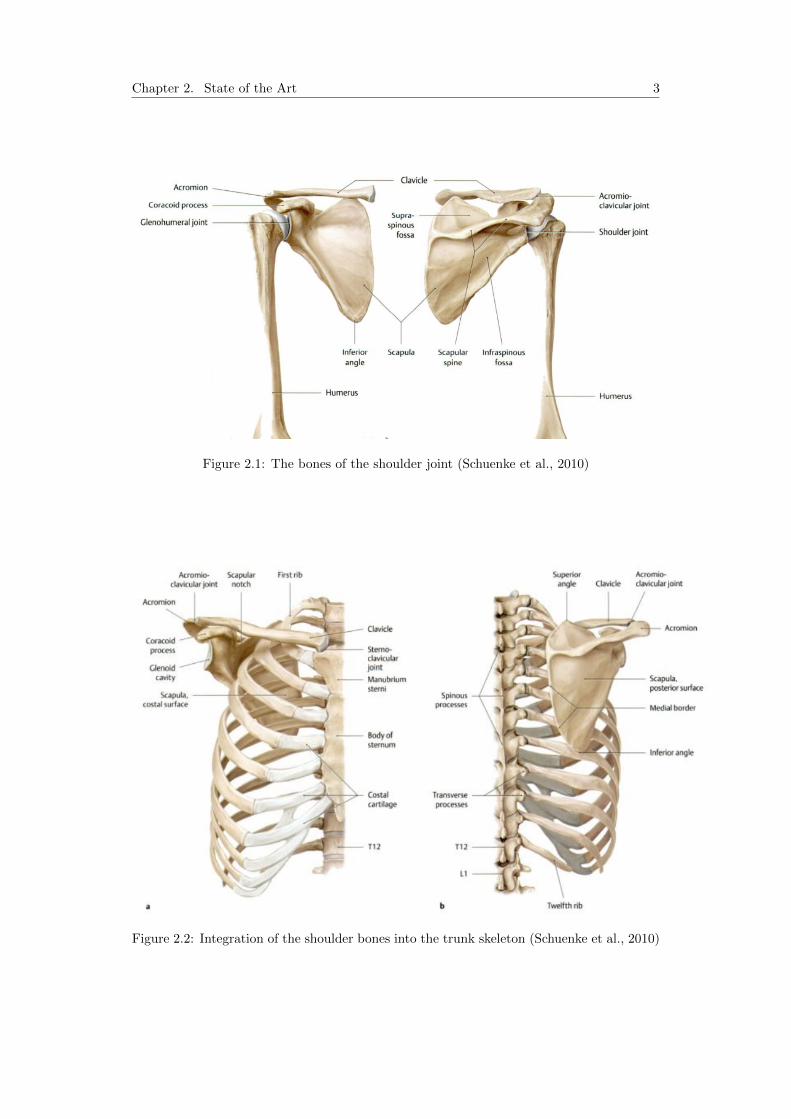
The human skeletal system is made up of 206 bones. The skeleton’s purpose is to protectthe body’s major organs and to allow motion and force transmission. A bone is composedof two types of tissue, cortical and trabecular bone. For a long bone, the trabecular bonetissue is located at the ends of the bone and in its center. The trabecular bone has a spongystructure, which allows a good distribution of the loads. The cortical bone forms the wallsof the central part of the bone. It is more dense and can take high constraints. The bonesform joints with each other to allow movement. At the joint interfaces cartilage reduces thefriction in the joint. The bones are held together by ligaments. (Pioletti, 2013) The mainbones in the shoulder are the humerus (upper arm bone), the scapula (shoulder blade) andthe clavicle (collarbone) (cf. Figure 2.1).The humerus is the longest bone of the upper extremities. In the section closest to theshoulder joint the head, a spheroid ariculation surface, and the greater and lesser tuberosityare located. The tuberosity serves as an attachment site for both ligaments and tendons.The scapula is a thin triangular bone lying on the posterior side of the thorax. The scapulahas several processes: The coracoid, spine, acromion and glenoid process. These processesserve as both origin and insertion site for multiple muscles. The clavicle connects the trunkto the other bones in the shoulder . The bone has a double curve along its long axis. It alsoserves as a site for muscle attachment as well as for protection of underlying neurovascularstructures. (Terry and Chopp, 2000)

These three bones are integrated into the skeleton of the trunk, meaning the sternum, therips and the vertebra. This construct can be seen in Figure 2.2. In this project the assemblyof these bones is called shoulder complex.

2

Chapter 2. State of the Art 3

Figure 2.1: The bones of the shoulder joint (Schuenke et al., 2010)

Figure 2.2: Integration of the shoulder bones into the trunk skeleton (Schuenke et al., 2010)


Bones of the shoulder complex are linked by several joints. The major joint is the gleno-humeral joint, which is mostly referred to as the shoulder joint. It is a synovial ball andsocket joint and involves articulation between the proximal head of the humerus and a shal-low socket in the scapula called glenoid fossa (more commonly glenoid cavity). Due to thesmall joint socket the shoulder is a very mobile joint. However, due to the same reason thestability in the shoulder can be an issue. (Terry and Chopp, 2000)There are further joints in the shoulder complex, such as the sternoclavicular joint betweenthe sternum and the clavicle and the acromioclavicular joint between the acromion, a con-tinuation of the scapular spine, and the clavicle. Furthermore, there is the scapula-thoracicjoint between the scapula and the thorax.

2.1.2 Muscles

The muscles are the engine of the musculoskeletal system. Muscles generate force, stiffenthe joints, move and thermoregulate the human body. They can be seen as a machine thatconverts chemical energy into mechanical work as well as heat. Skeletal muscles account forapproximately 40% of the body weight and are thus the largest organ of the body. Generally,a tendon attaches the muscle to the bone. (Pioletti, 2013)The shoulder complex is spanned by 16 muscles. The shoulder muscles can be categorisedwith a compromise between topographical and functional considerations. The shoulderjoint muscles are defined as the muscles that span over the glenohumeral joint, including therotator cuff muscles as well as the more superficial muscles. The complete list can be seenin Table 2.1. The rest are muscles that have migrated from the trunk (cf. Table 2.2). All ofthese muscles belong to the previously defined shoulder complex.

1. Muscles of the shoulder jointPosterior muscle groupSupraspinatus (rotator cuff)Infraspinatus (rotator cuff)Teres minor (rotator cuff)Subscapularis (rotator cuff)DeltoidLatissimus dorsiTeres majorAnterior muscle groupPectoralis majorCoracobrachialis

Table 2.1: Functional-topographical classification of shoulder muscles (Schuenke et al., 2010)

2. Muscles migrated from the trunkShoulder muscles that have migrated from the headTrapeziusPosterior muscles of the trunk and shoulderRhomboid majorRhomboid minorLevator scapulaeAnterior muscles of the trunk and shoulderSubclaviusPectoralis minorSerratus anterior

Table 2.2: Functional-topographical classification of shoulder muscles (Schuenke et al., 2010)


Origin and insertion

Every muscle has an origin and an insertion area. The origin of a muscle is the point ofattachment that remains relatively fixed during contraction. The muscle inserts on to thebone that is moved by the contraction of the muscle. For the 16 muscles of interest acomprehensive table is in Appendix A where the origin and insertion as well as their mainfunction is specified.

Rotator cuff muscles

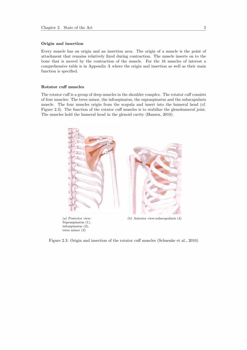
The rotator cuff is a group of deep muscles in the shoulder complex. The rotator cuff consistsof four muscles: The teres minor, the infraspinatus, the supraspinatus and the subscapularismuscle. The four muscles origin from the scapula and insert into the humeral head (cf.Figure 2.3). The function of the rotator cuff muscles is to stabilize the glenohumeral joint.The muscles hold the humeral head in the glenoid cavity (Hansen, 2010).

(a) Posterior view:Supraspinatus (1),infraspinatus (2),teres minor (3)

(b) Anterior view:subscapularis (4)

Figure 2.3: Origin and insertion of the rotator cuff muscles (Schuenke et al., 2010)


Deltoid muscle

The deltoid is a superficial muscle in the shoulder complex that gives the shoulder itsrounded form. The muscle has three sections, an anterior part, a medial part and a posteriorpart. They originate from three different locations, the clavicle, the acromial process andthe scapular spine respectively. They insert all together into the deltoid tuberosity of thehumerus. (Terry and Chopp, 2000)The deltoid muscle moves the shoulder joint. The middle part is responsible for the abduc-tion of the arm at the shoulder. The anterior part flexes and medially rotates the arm andthe posterior part extends and laterally rotates the arm at shoulder. (Hansen, 2010)

Figure 2.4: Deltoid muscle: Anterior (1), medial (2), posterior (3) (Schuenke et al., 2010)

2.2 Anatomical Reconstruction

An anatomical reconstruction is used to reconstruct a biological form, such as bones ormuscles. An anatomical reconstruction can be done using different data sources such ascomputed tomography (CT) or Magnetic Resonance Imaging (MRI). The MRI or CT scanscontain cross sectional images of the tissue. These images are segmented one by one tohighlight the 3D anatomical structures. A software, such as Amira, is necessary to visualisethe segmented data. Amira is 3D software platform for visualisation, manipulation andunderstanding data from different imaging modalities. For more detail on the Amira softwarerefer to Amira online (May 2014).


2.3 Kinematic Modelling

Kinematics describes the motion of objects. The kinematics of a multi-link system specifiesthe position, speed and acceleration of the reference frame of a segment. A map to describethese transformations has to be calculated, which is called the kinematic model (Burri andBleuler, 2013).

2.3.1 Definitions

Kinematic chain

A kinematic chain is an assembly of rigid bodies linked together by joints. The Figure 2.5shows a chain with two segments (L1 and L2) and two joints.

Figure 2.5: A simple kinematic chain (Burri and Bleuler, 2013)

Generalized coordinates

A set of generalized coordinates, also called joint variables, describe the joint space. Theydescribe the displacement of the reference frames of the segments (position or angle). Thesevariables are commonly represented by q (cf. Figure 2.5). The speed and the acceleration arenoted respectively q(t) and q(t). There is one generalized coordinate per degree of freedom(DOF) of the chain.

Operational coordinates

The operational coordinates describe what the end-effector of the kinematic chain does inthe world reference frame. If the world reference is in Cartesian coordinates the operationalcoordinates are (x, y, z).


Kinematic models

The purpose of the kinematic model, also called geometric model, is to establish the linkbetween the joint variables and the operational coordinates. It provides the mathematicaltools to transform from one set of variables to the other.

The forward kinematic model, also direct geometric model, is a set of kinematic equations.These equations compute the position of the end-effector in the world reference frame fromthe generalized coordinates. In other words, they express the operational coordinates (x, y, z)as a function of the generalized coordinates (q1, q2, ..., qn) (cf. Figure 2.6).

Figure 2.6: Forward kinematics (Burri and Bleuler, 2013)

Inverse kinematics, also inverse geometric model, uses the kinematic equations to determinethe generalized coordinates that provide a desired position of the end-effector in the worldreference frame. Hence, express the generalized coordinates (q1, q2, ..., qn) as a function ofthe operational coordinates (x, y, z) (cf. Figure 2.7).

Figure 2.7: Inverse kinematics (Burri and Bleuler, 2013)

2.3.2 Joint Coordinate System for the Shoulder Complex

In order to standardize the description of joint motion the Society of Biomechanics (ISB)has proposed a set of local coordinate systems (LCS). The following section gives a briefreview of this standardized description, for more detail refer to Wu et al. (2005): First a setof bony landmarks for the shoulder complex was defined (cf. Table 2.3).


Thorax C7: Spinous process of the 7th cervical vertebraT8: Spinal porcess of the 8th thoracic vertebraIJ: Deepest point of suprasternal notchPX: Xiphoid process, most caudal point on the sternum

Clavicle SC: Most ventral point on the sternoclavicular joint

AC:Most dorsal point on the acromioclavicular joint (sharedwith the scapula)

Scapula TS:Root of the spine, midpoint of the triangular surface onmedial border of the scapula in line with the scapular spine

AI: Inferior angle, most caudal point of the scapulaAA: Acromial angle, most laterodorsal point of the scapulaPC: Most ventral point of processus coracoideus

Humerus GH:Glenohumeral rotation center, estimated by regression ormotion recordings

EL: Most caudal point on lateral epicondyleEM: Most caudal point on medial epicondyle

Table 2.3: Anatomical landmarks: Thorax, clavicle, scapula and humerus. (Wu et al., 2005)

The next step is to define the coordinate system per body segment, here for the thorax, theclavicle, the scapula and the humerus (cf. Table 2.4).With these local coordinate systems the motion of the shoulder joint can be described. Tostandardize the motion of the shoulder, it was decided that Euler angles should be used todescribe all rotations. The proposed standardization suggests that the coordinate systemsof the proximal and distal body segment in question are initially aligned to each other. Thisalignment is obtained by the introduction of anatomical orientations of these coordinatesystems. When a rotation occurs, the rotation of the distal coordinate system should bereported with respect to the proximal coordinate system. If both coordinate systems arealigned the standardized sequence of rotation is the following: the first rotation around oneof the common axes, the second rotation around the axis of the moving coordinate systemand the third around a rotated axis of the moving coordinate system. To describe the jointdisplacement, a common point in both the distal and proximal coordinate systems should betaken. Such a point could be for example the initial rotation center. To represent true jointmotion, the displacement should be described with respect to the axes of the coordinatesystem of the segment directly proximal to the moving segment. (Wu et al., 2005)


Thorax coordinate system - XtYtZt

Ot: The origin coincident with IJ.

Yt:The line connecting the midpoint be-tween PX and T8 and the midpoint be-tween IJ and C7, pointing upwards.

Zt:The line perpendicular to the planeformed by IJ,C7 and the midpoint be-tween PX and T8, pointing to the right.

Xt:The common line perpendicular to theZt and Yt axis, pointing forwards.

Clavicle coordinate system - XcYcZc

Oc: The origin coincident with SC.

Zc:The line connecting SC and AC, point-ing to AC.

Xc:

The line perpendicular to Zc and Yt,pointing forward. Note that the Xc-axis is defined with respect to the verti-cal axis for the thorax(Yt-axis) becauseonly two bony landmarks can be dis-cerned at the clavicle.

Scapula coordinate system - XsYsZs

Os: The origin coincident with AA.

Zs:The line connecting TS and AA, point-ing to AA.

Ys:

The line perpendicular to the planeformed by AI, AA, and TS, pointing for-ward. Note that because of the use ofAA instead of AC, this plane is not thesame as the visual plane of the scapulabone.

Ys:The common line perpendicular to theXs- and Zs- axis, pointing upwards.

Humerus coordinate system - XhYhZh

Oh: The origin coincident with GH.

Yh:The line connecting GH and the mid-point of EL and EM, pointing to GH.

Xh:The line perpendicular to the planeformed by EL, EM, and GH, pointingforward.

Zh:The common line perpendicular to theYh- and Zh-axis, pointing to the right.

Table 2.4: Local coordinate systems for the shoulder complex. (Wu et al., 2005)


2.3.3 Kinematic Model of the Shoulder Complex

In biomechanics, kinematics can be used to describe the motion of the human skeleton. Thehuman skeleton can be seen as segments linked together by different joints. In the humanbody different kinds of joints exist with varying degrees of freedom (DOF).In the following section a brief review of the kinematic model of the shoulder complex ispresented, for more detail please refer to Ingram et al. (2012). When building the kine-matic chain of the shoulder complex the segments considered are the thorax, the clavicle,the scapula and the humerus. The segments are linked through the sternoclavicular joint(SC), the acromioclavicular joint (AC) and the glenohumeral joint (GH). For the generalmodel each of these joints is considered as an ideal spherical joint with three DOF. The lastjoint to consider is the scapulo-thoracic joint (ST), which is modelled using point-to-surface-constraints. With these assumptions the kinematic chain has a total of 7 DOF.To build the kinematic model, the joint coordinates as well as the reference frames for thesegments have to be defined. The standardized definition described in Section 2.3.2 is used.

The Figure 2.8 shows the shoulder complex with the kinematic chain, the bony landmarks,the joint reference system and coordinates. The notation used for the local origin andreference system is Oi, ei1, ei2, ei3, with the indices i = t, c, s, h for thorax, clavicle, scapulaand humerus. The absolute reference frame is placed at IJ.

Figure 2.8: The Shoulder complex:Kinematic chain and the JCS (Ingram et al., 2012)

In the zoomed detail in Figure 2.8 the rotations around the reference system at the AC jointare shown. To describe these rotations a vector of three coordinates for each segment isused:

xi = (θi1 θi2 θ

i3) ∈ χi ⊂ R3 i = t, c, s, h (2.1)

These are the generalized coordinates and χi is the bone configuration space.A point on a bone or segment can be described as:

pi = (pi2 pi2 p

i3) ∈ Wi ⊂ R3 i = t, c, s, h (2.2)


The workspace W attributed to each bone is equal to the cartesian coordinate space of thelocal reference frame. In order to be able to compute a point pi in the absolute workspacea set of maps has to be defined:

ξj : Wj →Wt

Pj → ξj(pj) = Rjpj, j = c, s, h(2.3)

The rotation matrix Rj is constructed using the joint coordinates. This set of equations isthe forward kinematic model for the shoulder complex. The inverse model is described bythe inverse of this map.

2.4 Dynamic Modelling

The dynamic modelling of a multi-link system describes the effects of external forces ortorques on the motion of a body. The dynamic model is calculated using either the Newton-Euler or the Lagrangian approach (Burri and Bleuler, 2013).

2.4.1 Definitions

Generalized forces

A generalized force is associated with each generalized coordinate defined earlier. They canbe either forces or torques and are denoted Γ(t).

Dynamic models

The direct dynamic model describes the position, speed and acceleration of the end-effectoras a function of the generalized forces in the system, q(t) = fD(Γ(t)) (cf. Figure 2.9).

Figure 2.9: Direct dynamic model (Burri and Bleuler, 2013)

The inverse dynmamic model is used to compute the torques necessary to reach a certainposition, speed and acceleration of the end-effector, Γ(t) = fI(q, q, q) (cf. Figure 2.10).

Figure 2.10: Inverse dynamic model (Burri and Bleuler, 2013)


2.4.2 Dynamic Model of the Shoulder Complex

This section describes the dynamic model of the shoulder complex, for more detail cf. Ingramet al. (2012). The dynamic model of the shoulder complex is obtained using the Langrangianmechanics and the joint coordinates xs. Each bone has a mass Mi and an inertia Ii (i = c,s, h) attached to the bone’s center of gravity. The dynamic equation is given as:

M(xs)xs + h(xs, xs) = fext (2.4)

where M(xs) is the dynamic inertia matrix and h(xs, xs) is a vector containing the internaldynamics. The vector fext is the generalized external force.The model includes 16 muscles which are divided into 28 segments. The segments arechosen according to anatomical criteria. The generalized external forces due to the musclesare calculated as follows:

fmscext =

∑pm × fm = P F (2.5)

where P is the 9× 28 moment arm matrix and F is the muscle force for each segment. Thematrix P has one column for each muscle segment, and there are 9 rows because for eachreference frame (clavicle, scapula and thorax) the moment arms are given. The dynamicmodel of the shoulder complex is given by the differential algebraic equations:

M(xs)xs = PF − h(xs, xs) (2.6)

2.5 Muscle Force Estimation

When estimating muscle forces in a biomechanical model a redundancy problem occurs.The redundancy problem is due to an over constraint set of equations of motion: The threeequations for the moment equilibrium have as many unknowns as there are muscle forces,leading to an infinite number of solutions for this set of equations. With the help of anoptimisation process and a suitable optimisation criteria a solution can be found.

2.5.1 Null-space Optimization

An optimization in mathematics is a process to find the most suitable solution out of all thepossible solutions according to a given criteria. For the shoulder model in this project thecriteria is:

Execute a given movement using minimal muscle stresses.

This criteria gives the additional equation necessary to solve the redundancy problem. So theoptimal solution within the null-space can be found. The null-space describes the solutionarea of the given problem, meaning all the possible solutions.


2.5.2 Application for Shoulder Model

Considering a joint motion which is defined by xs(t), xs(t) and xs(t), the generalized muscleforces can be defined by inverse dynamics as follows:

fmscext = P F = M(xs)xs + h(xs, xs) (2.7)

The muscle force has to be positive and a maximum strength constraint is defined:

0 ≤ F ≤ FMAX (2.8)

To find a solution, the problem is defined as an optimization problem as in Equation 2.9.Where g(F ) is the cost function defined as the mean square of the muscle stresses (cf. 2.10).

min g(F )

s.t. 0 ≤ F ≤ FMAX

fmscext = P F

(2.9)

g(F ) =

n∑i=1

(Fi/Ai)2

n(2.10)

In the cost function n is equal to the number of muscle forces that are to be computed andA is the physiological cross sectional area. For more detail refer to Ingram et al. (2012).

2.6 Musculoskeletal Joint Model in Matlab

The shoulder model was built using an existing approach (Ingram et al., 2012). The modelconsists of a preprocessor, that generates geometry and movement data, and a solver whichruns the optimization process to compute muscle and joint reaction forces.

2.6.1 Bones

The anatomical data to describe the bones in the numerical model come from a recon-struction of MRI images in Amira. The MRI images were taken from a young and healthyindividual. The definition of the bony landmarks and standardized definition of joint motionand local coordinate systems is taken from (Wu et al., 2005).

2.6.2 Muscles

In the existing numeric model the muscles are modelled as cables. As mentioned earlier,there are 16 muscles in the shoulder complex. These muscles are separated into 28 segments,chosen according to anatomical and topographical criteria. For example the deltoid muscleis split up in 3 segments according to their different origin locations.In the currently used Matlab program one cable per segment is computed. To define onecable, an origin and an insertion point has to be defined. Furthermore, the reference framesof those points have to be specified. For some muscle segments it is necessary to definesupplementary points called Via points. The cable passes through these points in order tohave the correct lever arm. If necessary two Via points can be defined, one close to theinsertion (Via A point) and one close to the origin (Via B point).


To further improve the anatomical representation of a muscle, the cable is guided alonga wrapping object. The wrapping objects are different kinds of cylinders. Three types ofwrapping object exist and are represented in the Table 2.5. For some segments no objectis necessary. For each type of wrapping object, its center, its reference frame, its diameterand its z-axis direction has to be specified.

Wrapping Objects

1 cylinder: 2 cylinders Cylinder with demi sphere’single’ ’double’ ’stub’

Table 2.5: Wrapping objects

The schematic in Figure 2.11 illustrates the path a cable has to follow.

Figure 2.11: Illustration of cable path


2.7 Geometry

2.7.1 Straight Line

Two points are necessary to define a straight line. Assuming the line passes through thepoint A and B, and the corresponding vectors are:

~a =

a1a2a3

, ~b =

b1b2b3

(2.11)

The parametrised line that passes through these two points is defined as:

r(t) = ~a+ t(~b− ~a) (2.12)

2.7.2 Spline Interpolation

The following section contains an introduction to spline interpolations, for more detail referto Barbic (2011): A spline is a piecewise polynomial, where many low degree polynomials areused to interpolate the control points. Cubic splines use cubic polynomials to interpolate.They are the lowest order polynomials that interpolate 2 points and allow the gradient ateach point to be defined (C1 continuity is possible).There are different types of splines. Here the Catmull-Rom spline, a special case of the cubicHermite spline and is explained first. A cubic Hermite spline is a spline where each segmentbetween two control points is a third-degree polynomial specified in 3D by the position andtangent vectors at the end points of the interval [0, 1] (cf. Figure 2.12).

Figure 2.12: Hermite spline specification (Barbic, 2011)

Four constraints can be defined, the position and the tangent vectors of the two end points:

p(0) = p1 = (x1, y1, z1)

p(1) = p2 = (x2, y2, z2)

p′(0) = p1 = (x1, y1, z1)

p′(1) = p2 = (x2, y2, z2)

(2.13)

The cubic form p(u) = au3 + bu2 + cu+d, is assumed which gives 4 unknowns a, b, c, d andleads to a linear system with 12 equations and 12 unknowns. After solving, the followingform is obtained:

[x(u) y(u) z(u)

]=[u3 u2 u 1

] 2 −2 1 1−3 3 −2 −10 0 1 01 0 0 0

x1 y1 z1x2 y2 z2x1 y1 z1x2 y2 z2

(2.14)


where (x, y, z) is a point on the spline segment, the parameter u varies between 0 and 1 andthe last matrix is the control matrix containing the information about the control points. Tohave a multi segment Hermite spline the joining ends of two segments have to have machingpositions and tangent vectors.As mentioned, the Catmull-Rom spline is a special case of the Hermite splines. For theCatmull-Rom spline the tangent at the control point pi is set to s ∗ (pi+1 − pi−1), where sis the tension parameter. This parameter determines the magnitude of the tangent vectorat pi. The two end points are used as extra control points at both ends of the spline todefine the tangents there. So the spline segment between the control points pi and pi+1 iscompletely defined by pi−1, pi, pi+1 and pi+2.The parametrized equation for a Catmull-Rom spline segment is in Equation 2.15. Theparameter s is typically set to 0.5. The matrix depending on the parameter s is called basisand the matrix with the four points is called control matrix.

[x(u) y(u) z(u)

]=[u3 u2 u 1

] −s 2− s s− 2 s2s s− 3 3− 2s −s−s 0 s 00 1 0 0

x1 y1 z1x2 y2 z2x3 y3 z3x4 y4 z4

(2.15)

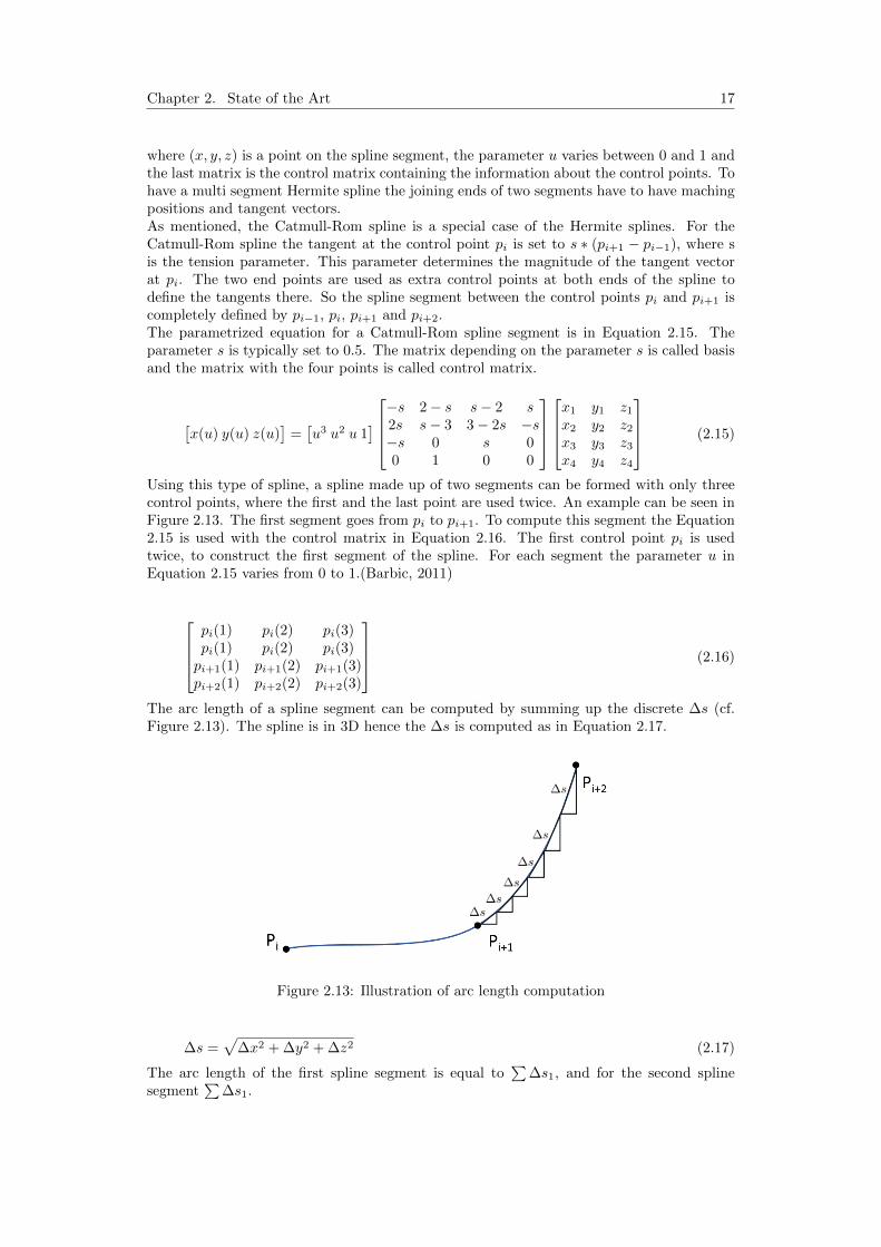
Using this type of spline, a spline made up of two segments can be formed with only threecontrol points, where the first and the last point are used twice. An example can be seen inFigure 2.13. The first segment goes from pi to pi+1. To compute this segment the Equation2.15 is used with the control matrix in Equation 2.16. The first control point pi is usedtwice, to construct the first segment of the spline. For each segment the parameter u inEquation 2.15 varies from 0 to 1.(Barbic, 2011)

pi(1) pi(2) pi(3)pi(1) pi(2) pi(3)pi+1(1) pi+1(2) pi+1(3)pi+2(1) pi+2(2) pi+2(3)

(2.16)

The arc length of a spline segment can be computed by summing up the discrete ∆s (cf.Figure 2.13). The spline is in 3D hence the ∆s is computed as in Equation 2.17.

Figure 2.13: Illustration of arc length computation

∆s =√

∆x2 + ∆y2 + ∆z2 (2.17)

The arc length of the first spline segment is equal to∑

∆s1, and for the second splinesegment

∑∆s1.

Chapter 3

Methods

The Matlab model evaluates the muscle force per muscle segment necessary for a givenmovement. In the existing model there is one cable for each muscle segment. The goal is toimplement the possibility to have multiple cables per segment. To achieve this goal, a newpreprocessor for this model is implemented which allows to generate the data for the bonesand configure the muscle cables before the solver computes the forces.

3.1 Muscle Modelling

A muscle inserts and originates from an area on a bone as schematized in Figure 3.1.

Figure 3.1: Schema of a muscle

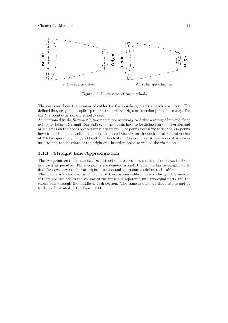
In the current model these areas are approximated with one point. In order to have multi-ple cables per segment this area has to be approximated differently. Two new approachesto approximate the insertion and origin areas are implemented for this project. The firstmethod consists in approximating the insertion and origin areas with a straight line as inFigure 3.2(a). For the second method, these areas are approximated with a Catmull-Romspline (cf. Figure 3.2(a)).

18

Chapter 3. Methods 19

(a) Line approximation (b) Spline approximation

Figure 3.2: Illustration of two methods

The user can chose the number of cables for the muscle segments at each execution. Thedefined line, or spline, is split up to find the defined origin or insertion points necessary. Forthe Via points the same method is used.As mentioned in the Section 2.7, two points are necessary to define a straight line and threepoints to define a Catmull-Rom spline. These points have to be defined on the insertion andorigin areas on the bones on each muscle segment. The points necessary to set the Via pointshave to be defined as well. The points are placed visually on the anatomical reconstructionof MRI images of a young and healthy individual (cf. Section 2.2). An anatomical atlas wasused to find the locations of the origin and insertion areas as well as the via points.

3.1.1 Straight Line Approximation

The two points on the anatomical reconstruction are chosen so that the line follows the boneas closely as possible. The two points are denoted A and B. The line has to be split up tofind the necessary number of origin, insertion and via points to define each cable.The muscle is considered as a volume, if there is one cable it passes through the middle.If there are two cables the volume of the muscle is separated into two equal parts and thecables pass through the middle of each section. The same is done for three cables and soforth, as illustrated in the Figure 4.11.


(a) One cable (b) Two cables

(c) Three cables

Figure 3.3: The cables distributed on a straight line

Looking at Figure 4.11, it is evident that if there is one cable it starts at 1/2 of the line, ifthere are two cables they start at 1/4 and 3/4 of the line. The Figure 3.4 shows the two

points A and B and their associated vectors ~a and ~b. To find a point C on the line theEquation 3.1 is used.

(a) One point on a line (b) Two points on a line

Figure 3.4: Method to split straight line

~c = ~a+ λ(~b− ~a) (3.1)

The parameter λ depends on the number of cables per muscle segment. The Table 3.1 showsthe parameter depending on the number of cables. The parameter λ can be determined forany number of cables with the Equation 3.2.

λ =2 ∗ Curr Muscle Cable − 1

2 ∗ Cable Array(Curr Muscle Segm)(3.2)


# cables first cable 2nd cable 3rd cable 4rd cable 5th cable1 λ = 1/22 λ = 1/4 λ = 3/43 λ = 1/6 λ = 3/6 λ = 5/64 λ = 1/8 λ = 3/8 λ = 5/8 λ = 7/85 λ = 1/10 λ = 3/10 λ = 5/10 λ = 7/10 λ = 9/10

Table 3.1: Row structure for the cable information cell array

3.1.2 Catmull-Rom Spline Approximation

When using a spline to approximate the origin and insertion areas the distribution of thecables is done similarly to the line approximation. The muscle is again considered as avolume and is split up. The Figure 3.5 shows the distribution of the cables on a spline.

(a) One cables (b) Two cables

(c) Three cables

Figure 3.5: The cables distributed on a Spline

To find any points on a spline, its parametrized equation can be used. The parametrizedequation is recalled here:

[x(u) y(u) z(u)

]=[u3 u2 u 1

] −s 2− s s− 2 s2s s− 3 3− 2s −s−s 0 s 00 1 0 0

x1 y1 z1x2 y2 z2x3 y3 z3x4 y4 z4

(3.3)

Each segment of the spline is defined by this parametrized equation and any point on thespline segment can be found by choosing the parameter u between 0 and 1. To split up thespline as in Figure 3.5 the arc length of the spline can be used. The total arc length of aspline, made up of two segments, is equal to the sum of the arc length of each segment:

total arc length =∑

∆s1 +∑

∆s2 (3.4)

The computations of the arc length of one segment∑

∆s is described in Section 2.7. Aspline with two segments is illustrated in Figure 3.6.


Figure 3.6: Arc length for a spline with two segments

As mentioned, the parameter u has to be determined to find a point on the spline segment.Since there are two spline segments there is a separate parameter for each segment, u1 andu2. For each segment the parameter goes from 0 to 1, as illustrated in Figure 3.7

Figure 3.7: Parameter u for a spline with two segments

Once the total arc length of the spline is known, the parameter λ is used to split up the totalarc length. Hence the target arc length for each desired point on the spline can be found:

target arc lenght = λ ∗ total arc length (3.5)


From the target arc length it can be determined on which spline segment the point is. Inthe case that the target arc lenght is smaller than

∑∆s1 the desired point C is on the first

segment. To find the point C, the parameter u1 has to be determined and entered in thethe parametrized equation of the first spline segment. The parameter u1 can be computedwith the ratio of length in the first segment:

u1 =target arc lenght∑

∆s1(3.6)

If the target arc lenght is bigger than the the length of the first segment, the point C is onthe second segment of the spline. Hence the parameter u2 has to be computed and enteredin the parametrized equation of the second segment. The parameter u2 is determined asfollows:

u2 =target arc length−

∑∆s1∑

∆s2(3.7)

3.2 Preprocessor Program Structure

The structure of the new preprocessor can be seen in Figure 3.8.

Figure 3.8: Flow chart for the preprocessor

The PRE PROC MAIN.m file is the main file of the preprocessor, it controls the config-uration of the bone and muscle structure and plots the chosen cable in the visualisation.The Amira Raw.m file’s output is the muscle data needed for the chosen cable. The com-putation of the muscle data for all cables is coordinated by the file Cable Preprocessor.m.The cable preprocessor calls all functions necessary to compute the origin, insertion, Viapoint and wrapping data necessary for each cable. Before executing the code, the user canchoose how many cables should be computed per muscle segment. This is done by changingthe values in the array Cable Array. The array’s size is 28 × 1 and each row of the arraycorresponds to the number of cables in a muscle segment. Furthermore, the user chooseswhich cable of which segment should be drawn in the visualisation.


3.3 Data Structure

The data transfer from one function to the other is done via cell arrays. For one cable 13parameters are necessary. Therefore, all cell arrays dealing with the cable data have 13 rowsstructured as in Table 3.2.

Parameters for one muscle cableRow 1: Pv : Muscle OriginRow 2: Pref : Origin Reference frameRow 3: Sv : Muscle InsertionRow 4: Sref : Insertion Reference frameRow 5: Ov : Wrapping Object CenterRow 6: Oref : Wrapping Object Reference frameRow 7: Otype : Wrapping Object typeRow 8: Ozaxis : Wrapping Object z axis directionRow 9: R : Wrapping Object DiameterRow 10: Vav : Via Point A (Near Insertion)Row 11: Varef : Via Point A Reference SystemRow 12: Vbv : Via Point B (Near Origin)Row 13: Vbref : Via Point B Reference System

Table 3.2: Row structure for the cable data cell array

In the get Points Amira function the points from Amira are saved in cell arrays. The cellarrays have 28 columns, one for each muscle segment. There is one cell array for the inser-tion points, the origin points and the Via point.The get Wrapping Info.m function fills a cell array (size 13 × 28) with the wrapping in-formation and the different reference frames for each segment. The cell array Cable Datais the one that saves all the information for all cables. Its size depends on the total numberof cables. The total number of cables is the sum of all the elements in the Cable Array.Hence the size of the Cable Data cell array is 13× total number of cables.

3.4 Numerical Studies

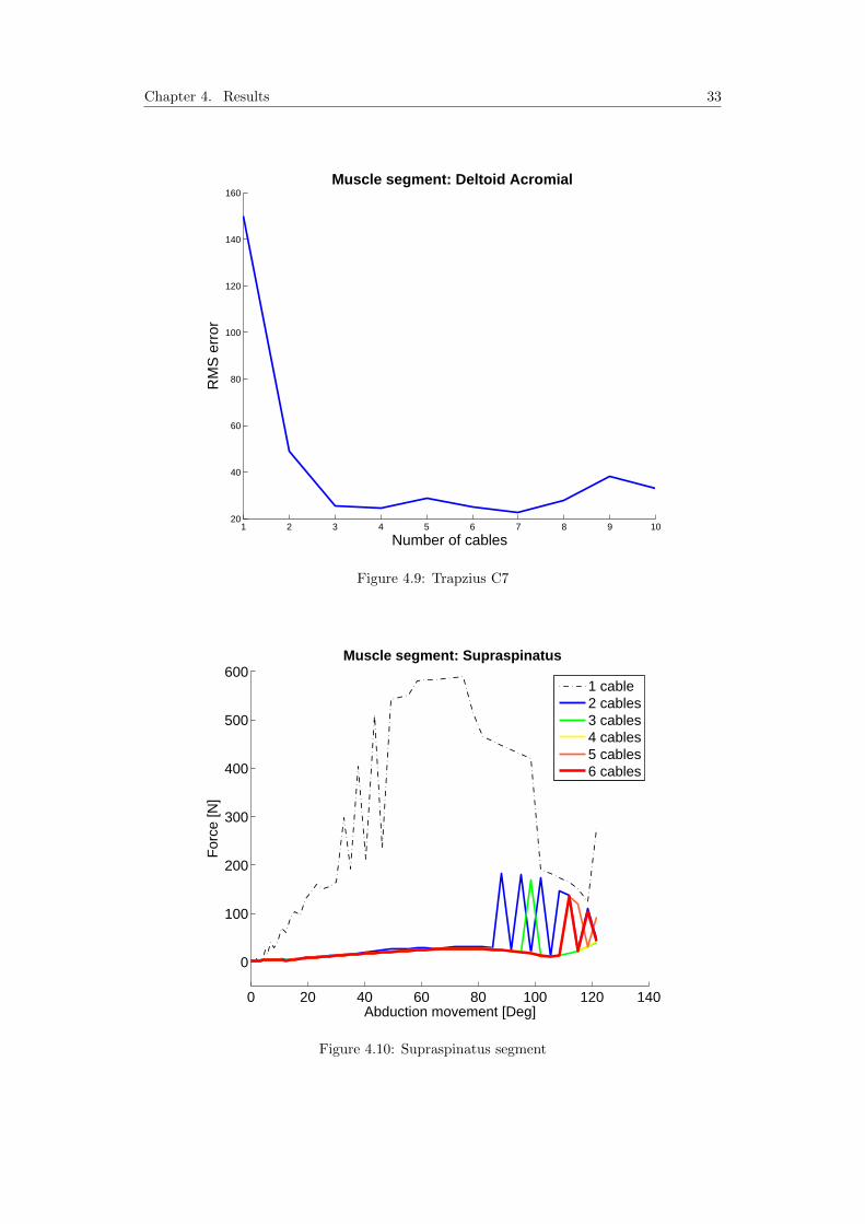
The new preprocessor has to be integrated in the existing solver in order that the muscleforces per cable can be computed. To get the muscle force per segment, the forces of allcables of that segment are summed up. The movement that is simulated for the first tests isthe abduction of the arm up to 120◦. The force can be plotted in function of the movementfor each segment. The goal is to determine how many cables per segment are necessary toget consistent results in the muscle force.First the muscle force necessary for the abduction, when the muscle is modelled as one cable,is computed. Then the number of cables per segment is increased and the computation is re-peated. The solver computes the force for each cable. To get a force for one muscle segmentthe forces per cable have to be added up. For each of the 28 muscle segments a graph can beplotted. Each graph will show the evolution of the force in a given muscle segment in func-tion of the movement. There is one curve per number of cables in each graph. The curvesfor the trapzius C7, deltoid acromial and supraspinatus will be analysed in detail. Thesethree muscle segments were chosen because they are important for the abduction movement.


To compare the results for the different number of cables, two indexes are used. The firstis the so called Smoothness Index. To determine the smoothness, the jumps of the curvehave to be evaluated. The jumps in each curve are counted and their height is measured.To count the number of jumps in a curve, the second order derivative is used. The secondorder derivative describes the curvature of a function, and per jump in the original curvethere is a peak in the second order derivative. The threshold for a change in the curve tobe categorised as a jump is defined at 5 Newton. The Smoothness Index is defined as thenumber of peaks

∑j multiplied with their average height H.

Smoothness Index = mean(H) ∗∑

j (3.8)

This gives an index for every number of cables per muscle segment. It shows whether thecurves get smoother after a certain number of cables.

The second index helps to determine how many cables are necessary to get consistent resultsof the muscle forces. The index used is the root mean square (RMS) error. The RMS errorbetween two consecutive number of cables is computed:

RMS error =√

(mean(data− estimate)2) (3.9)

With this index the difference between two consecutive curves can be evaluated. I.e. if thecurve for 3 and 4 cables are compared, the force curve for 4 cables is taken as the data andthe force curve for 3 cables is the estimate. If the RMS error gets smaller this means thatthe difference between the computed force per amount of cable decreases. Both indexes areplotted in graphs in function of the number of cables in a segment. The evolution of theseindexes is presented and then discussed in the following chapters of the report.

Chapter 4

Results

The first step is to compare the two methods to generate the muscle data. The comparisonbetween the line and the spline approximation is done visually. The Figure 4.1 shows theposterior part of the deltoid muscle once with the Line approximation (Figure 4.1(a)) andonce with the spline approximation (Figure 4.1(b)). The Figure 4.1(b) shows that the splinefollows the form of the bone more closely, which was to expect. All further simulations willbe done using the spline approximation.

(a) Line approximation (b) Spline approximation

Figure 4.1: Comparison between two approximation methods

In the following paragraphs the force curves for the muscle segments trapzius C7, deltoidacromial and supraspinatus are presented. The two indexes are computed and plotted forthese three segments. The force curves for the remaining muscle segments can be found inAppendix B.

The result for the trapezius C7 muscle segments, which originates from the 7th cervicalvertebra, can be seen in Figure 4.2.Per amount of cables there is one curve for the force evolution. The black dash-dot curverepresents the evolution of the force for one cable. The blue line represents the force for twocables. For the trapzius C7 segment, modelled with two cables, the force increases up toabout 80◦ of abduction. Afterwards, jumps appear in the force curve. The green line in thegraph shows the force using three cables, here the number of jumps decreases. Even if thenumber of cables is increased, there are still jumps in the curves but their height decreases.To quantify the observed jumps the Smoothness Index is computed. The second orderderivative can be seen in the Figures 4.3 for the trapzius C7 segment for one to six cables.

26

Chapter 4. Results 27

0 20 40 60 80 100 120 140

0

100

200

300

400

500

600 Muscle segment: Trapezius C7

Abduction movement [Deg]

For

ce [N

]

1 cable2 cables3 cables4 cables5 cables6 cables

Figure 4.2: Trapzius C7


0 20 40 60 80 100 120 140−50

0

50

100

150

200



For

ce [N

]

2 cables2nd derivative

(a) Two cables

0 20 40 60 80 100 120 140−50

0

50

100

150

200


Abduction movement [Deg]F

orce

[N]


(b) Three cables

0 20 40 60 80 100 120 140−50

0

50

100

150

200



For

ce [N

]


(c) Four cables

0 20 40 60 80 100 120 140−50

0

50

100

150

200



For

ce [N

]


(d) Five cables

0 20 40 60 80 100 120 140−50

0

50

100

150

200



For

ce [N

]


(e) Six cables

Figure 4.3: The second order derivative for the trapezius C7 muscle segment


For the trapezius C7 segment the Smoothness Index is calculated for one to 11 segmentsand is plotted against the number of cables. The plot can be seen in Figure 4.4. The indexdecreases up to 3 cables and then stabilizes, after 7 cables it starts to increase again.

1 2 3 4 5 6 7 8 9 10 110

100

200

300

400

500

600

700

800

900

1000 Muscle segment: Trapzius C7

Number of cables

Sm

ooth

ness

Inde

x

Figure 4.4: Smoothness Index for Trapzius C7

The RMS error is computed to see the difference between two consecutive number of cables.This has been done for the trapzius C7 segment and the plot for up to 11 cables can be seenin Figure 4.5.Here the same observation as before can be made. For the trapezius C7 segment the RMSerror decreases between 1 and 3 cables before it stabilizes.


1 2 3 4 5 6 7 8 9 100

10

20

30

40

50


Number of cables

RM

S e

rror


0 20 40 60 80 100 120 140

0

100

200

300

400

500

600 Muscle segment: Deltoid Acromial


For

ce [N

]


Figure 4.6: Deltoid acromial segment


0 20 40 60 80 100 120 140

0

100

200

300

400

500



For

ce [N

]


(a) One cable

0 20 40 60 80 100 120 140

0

100

200

300

400

500



orce

[N]


(b) Two cables

0 20 40 60 80 100 120 140

0

100

200

300

400

500



For

ce [N

]


(c) Three cables

0 20 40 60 80 100 120 140

0

100

200

300

400

500



For

ce [N

]


(d) Three cables

0 20 40 60 80 100 120 140

0

100

200

300

400

500



For

ce [N

]


(e) Three cables

Figure 4.7: The second order derivative for the deltoid acromial muscle segment


The Figure 4.6 shows the force for the middle part of the deltoid muscle, originating from theacromial process. The force for all number of cables increases up to about 80◦ where jumpsstart to occur. The second order derivatives in Figure 4.7 correspond to this observation.The Smoothness Index in Figure 4.8 decreases from 1 to 3 cables and stabilizes up to 7cables. With more then 7 cables the Smoothness Index increases again.

1 2 3 4 5 6 7 8 9 10 110

500

1000

1500

2000


Number of cables

Sm

ooth

ness

Inde

x

Figure 4.8: Smoothness Index for Trapzius C7

The RMS error for the deltoid acromial decreases up to 3 cables and then stabilizes as well.Again there is a slight increase after 7 cables.The Figure 4.10 shows the force evolution for the supraspinatus segment.The evolution of the Smoothness Index for the supraspinatus is similar to the previouslydiscussed segments. It decreases up to 3 cables, stabilizes and increases again after 7 cables.The RMS error for the supraspinatus decreases up to 4 cables and then stabilizes.


1 2 3 4 5 6 7 8 9 1020

40

60

80

100

120

140


Number of cables

RM

S e

rror


0 20 40 60 80 100 120 140

0

100

200

300

400

500

600 Muscle segment: Supraspinatus


For

ce [N

]


Figure 4.10: Supraspinatus segment


0 20 40 60 80 100 120 140−50

0

50

100

150

200



For

ce [N

]


(a) One cable

0 20 40 60 80 100 120 140−50

0

50

100

150

200



orce

[N]


(b) Two cables

0 20 40 60 80 100 120 140−50

0

50

100

150

200



For

ce [N

]


(c) Three cables

0 20 40 60 80 100 120 140−50

0

50

100

150

200



For

ce [N

]


(d) Three cables

0 20 40 60 80 100 120 140−50

0

50

100

150

200



For

ce [N

]


(e) Three cables

Figure 4.11: The second order derivative for the deltoid acromial muscle segment


1 2 3 4 5 6 7 8 9 10 110

100

200

300

400

500

600

700

800

900

1000 Muscle segment: Trapzius C7

Number of cables

Sm

ooth

ness

Inde

x

Figure 4.12: Smoothness Index for supraspinatus segment

1 2 3 4 5 6 7 8 9 100

10

20

30

40

50


Number of cables

RM

S e

rror

Figure 4.13: RMS error for the supraspinatus segment

Chapter 5

Discussion and Conclusion

The goal of the numerical study was to determine the minimal number of cables per musclesegment necessary to get consistent results for the muscle forces.A strong point of the musculoskeletal joint model used for the numerical studies is the factthat the model simulates all the muscles in the shoulder complex. Furthermore, the modelis dynamic and every movement of the shoulder can be simulated. An other advantage isthat the model is programmed on Matlab, which can be used on any operating system.However, the model has some limitations. The fact that the muscles were split up accordingto anatomical criteria can be seen as a limitation. The question is, whether this is the bestmethod to separate the muscles into segments. To estimate the muscle forces in the modelit would possibly be better to consider physiological criteria. Such as the innervation of themuscles or their function.There are the limitations of a 1D representation of muscles in general. A muscle is a verycomplex 3D structure in the human body. If the muscle is modelled as one cable, meaningas 1D, the line of action of the muscle is not exact. Furthermore, the distribution of thefibres is neglected and the interaction between different muscles and underlying structurescannot be taken into consideration. The advantage of the 1D model is its simplicity. It issimple to implement and the computational effort is small.For the numerical study conducted multiple cables per muscle segment were implementedand distributed on a spline. This could be seen as a 2D model of the muscle. Comparedto the 1D model, the 2D representation of a muscle represents the complex structure of themuscle more realistically. The line of action of the muscle is improved and the notion ofmuscle fibres is taken into account. However, it is still an approximation compared to the3D structure of the muscle.The force estimation is computed using an optimisation algorithm. The criteria used is:Execute a given movement with minimal muscle stresses. This is a purely mechanical cri-teria, which represents an other limitation of the model. By taking a mechanical criteriathe stabilizing functions of the muscles are not taken into consideration. With the currentcriteria only the muscle segments necessary for the movement are activated. However, thereare muscle segments that are not directly implied in the movement but stabilize the shoulderduring the execution of the movement. Instead of using the stress-based method to solvethe redundancy, the electromyography(EMG)-based method could be used, for more detailrefer to (Engelhardt et al., 2014).

36

Chapter 5. Discussion and Conclusion 37

As mentioned earlier, the 2D representation of the muscle is done either with a line or aspline method. The two methods to distribute several cables for one muscles segment werecompared in Section 4. When approximating an area on the bone with a straight line, theproblem is that the bone is not straight but has curves. For some origin and insertion areasthe line approximation would be sufficient, i. e. the insertion of the deltoid on the humerusis on a straight line. However, the origin of the deltoid acromial is on the scapular spinewhich makes a curve. So if this insertion site is approximated with a line, the line does notfollow the bone. With a spline approximation however, the spline can follow the curvatureof the bone.

The question to answer with the numerical study is: How many cables per muscle segmentare necessary to get consistent results of the muscle force?The results for the three muscle segments trapzius C7, deltoid acromial and supraspinatusare presented in the previous chapter. The computations for one cable per segment yieldinconsistent results. The problem is that the solver cannot find a solution within the opti-mization criteria if there is only one cable. This is due to the moment equilibrium at thesternoclavicular joint, which cannot be satisfied.To quantify the observations in the force graphs, two indexes are used. The SmoothnessIndex and the RMS error. The Smoothness Index quantifies the jumps observed in the forcecurves. The jumps can be explained with the used optimisation criteria. The solver tries tosatisfy the criteria at each movement step. The distribution of the force per muscle segmentis decided at each step to fulfil the criteria. If from one step to the other another segment iscloser to the optimal solution, there will be abrupt changes in the force which lead to jumpsin the curves. The RMS error quantifies whether the force curves converge to one resultwhen increasing the number of cables.When evaluating the indexes for the trapezius C7, the deltoid acromial and the supraspina-tus segment both the indexes decrease until the muscles are modelled with 3 to 4 cables.Then the indexes stabilize. For the Deloid Acromial the indexes increase again with morethan 7 cables. For the Trapezius C7 and the Supraspinatus the Smoothness Index increasesalso with more than 7 cables but the RMS error stays stable.The decreasing Smoothness Index indicates that both the number and height of the jumpsdecrease between 1 and 3 cables for all three segments. For more than 3 cables the indexis stabilized which means that the number or the height of the jumps do not change anymore. The decreasing RMS errors means that the difference between two consecutive cablenumbers decreases. If the RMS erros stabilizes the muscle forces have converged to oneresult. These observations lead to the conclusion that 3 or more cables are necessary to getconsistent results in the muscle forces.

However, the number of cables should not be increased to more than 7 cables because bothindexes start to increase again after 7 cables. This means that there are either more jumpsor higher jumps in the curves as well as a bigger difference between two consecutive cables.If the number of cables per segment is increased the computations get more complicated.Increasing the number of cables also increases the number of variables further in the alreadyover-constraint set of equations (c.f. Section 2.5). The computation of the null-space requiresa numerical matrix inversion which looses precision with increasing matrix sizes. Thus thequality of the solution will also decrease resulting in discontinuous force curves.

Chapter 5. Discussion and Conclusion 38

As the model is now, it is possible to estimate the muscle forces in the shoulder complexfor multiple cables per muscle segment. The adapted model will help to further understandthe complex kinematic system of the shoulder. The improved computation of muscle andjoint reaction forces will also help to further understand muscle coordination and articularmechanics. It is however possible to continue working and improving the musculoskeletaljoint model of the shoulder.A possible next step is to test the model with an alternative optimisation criteria, as men-tioned earlier. Furthermore, the results of the numerical studies can be compared to experi-mental data to validate the model. Another step is to further improve the modelling musclestructure. Now the muscles are modelled in 2D, the cables are distributed on a spline. Onecould try to model the muscles as close as possible to their 3D structure. Instead of approx-imating the areas on the bone with a spline or a line, it could be approximated by a finitenumber of points distributed on the area. For each cable a point among these points has tobe chosen according to a given algorithm.

5.1 Acknowledgement

At this point I would like to thank my assistant Christoph Engelhardt for his help andsupport during this semester project. I would also like to thank David Ingram for his workon the model which made it possible for me to test the newly implemented methods.

Bibliography

Amira online. May 2014. Amira homepage. http://www.vsg3d.com/amira/overview.

Barbic J., 2011. Script: CSCI 480 Computer Graphics. Georgia Institute of Technology(GT), Atlanta, Georgia.

Burri M. and Bleuler H., 2013. Lecture notes: Base de la robotique. Ecole polytechniquefederal de Lausanne (EPFL), Lausanne.

Engelhardt C., Malfroy Camine V., Ingram D., Muellhaupt P., Farron A., Pio-letti D. and Terrier A. 2014. Comparison of an emg-based and a stress-basedmethod to predict shoulder muscle forces. Computer Methods in Biomechanicsand Biomedical Engineering. URL http://www.scopus.com/inward/record.url?eid=

2-s2.0-84897353666&partnerID=40&md5=9e58b933723eed7bd9c30c04f3650047.

Hansen J., 2010. Netter’s Clinical Anatomy. Saunders Elsevier, Philadelphia. ISBN 978-1-4377-0272-9.

Ingram D., Muellhaupt P., Terrier A., Pralong E. and Farron A. 2012. Dynamical biome-chanical model of the shoulder for muscle-force estimation. Proceedings of the IEEERAS-EMBS International Conference on Biomedical Robotics and Biomechatronics. 407–412.

Pioletti D., 2013. Script: Biomechanics of the musculoskeletal system. Ecole polytechniquefederal de Lausanne (EPFL), Lausanne.

Schuenke M., Schulte E. and Schumacher U., 2010. Atlas of Anatomy: General Anatomyand Musculoskeletal System. Georg Thieme Verlag, Stuttgart. ISBN 978-1-60406-292-2.

Terry G. and Chopp T. 2000. Functional anatomy of the shoulder. Journal of Ath-letic Training. 35(3), 248–255. URL http://www.scopus.com/inward/record.url?eid=

2-s2.0-0347561430&partnerID=40&md5=f16331318751657e1392b43c1927c84c.

Wu G., Van Der Helm F., Veeger H., Makhsous M., Van Roy P., Anglin C., Nagels J.,Karduna A., McQuade K., Wang X., Werner F. and Buchholz B. 2005. Isb recom-mendation on definitions of joint coordinate systems of various joints for the reportingof human joint motion - part ii: Shoulder, elbow, wrist and hand. Journal of Biome-chanics. 38(5), 981–992. URL http://www.scopus.com/inward/record.url?eid=2-s2.

0-20144387878&partnerID=40&md5=0061c16426841273a89a29ca540b2283.

39

http://www.vsg3d.com/amira/overview

http://www.scopus.com/inward/record.url?eid=2-s2.0-84897353666&partnerID=40&md5=9e58b933723eed7bd9c30c04f3650047

http://www.scopus.com/inward/record.url?eid=2-s2.0-84897353666&partnerID=40&md5=9e58b933723eed7bd9c30c04f3650047

http://www.scopus.com/inward/record.url?eid=2-s2.0-0347561430&partnerID=40&md5=f16331318751657e1392b43c1927c84c

http://www.scopus.com/inward/record.url?eid=2-s2.0-0347561430&partnerID=40&md5=f16331318751657e1392b43c1927c84c

http://www.scopus.com/inward/record.url?eid=2-s2.0-20144387878&partnerID=40&md5=0061c16426841273a89a29ca540b2283

http://www.scopus.com/inward/record.url?eid=2-s2.0-20144387878&partnerID=40&md5=0061c16426841273a89a29ca540b2283

Appendix A

Origin and Insertion forShoulder Muscles

A.1 Muscles of the Shoulder Joint

40

Appendix A. Origin and Insertion for Shoulder Muscles 41

Mu

scle

Image

Ori

gin

Inse

rtio

nM

ain

acti

on

Su

pra

spin

atu

sS

up

rasp

inou

sfo

ssa

ofsc

ap

ula

Su

per

ior

face

ton

gre

ate

rtu

ber

cle

of

hu

mer

us

Hel

ps

del

toid

abd

uct

arm

at

shou

lder

an

dact

sw

ith

rota

tor

cuff

mu

scle

s

Infr

asp

inat

us

Infr

asp

inou

sfo

ssa

ofsc

ap

ula

Mid

dle

face

ton

gre

ate

rtu

ber

cle

of

hu

mer

us

Late

rall

yro

tate

sarm

at

shou

lder

;h

elp

sto

hold

hea

din

gle

noid

cavit

y

Ter

esm

inor

Late

ral

bord

erof

scap

ula

Infe

rior

face

ton

gre

ate

rtu

ber

cle

of

hu

mer

us

Late

rall

yro

tate

sarm

at

shou

lder

;h

elp

sto

hold

hea

din

gle

noid

cavit

y

Su

bsc

apu

lari

sS

ub

scap

ula

rfo

ssa

ofsc

ap

ula

Les

ser

tub

ercl

eof

hu

mer

us

Med

iall

yro

tate

sarm

at

shou

l-d

eran

dad

du

cts

it;

hel

ps

toh

old

hea

din

gle

noid

cavit

y


Del

toid

:

Ante

rior

par

t(1)

Mid

dle

par

t(2

)P

oste

rior

par

t(3

)

Late

ral

thir

dof

clav

icle

,ac

rom

ion

an

dsp

ine

of

scap

ula

Del

toid

tub

erosi

tyof

hu

mer

us

Anteriorpart:

Fle

xes

an

dm

edia

lly

rota

tes

arm

at

shou

lder

Middle

part:

Ab

du

cts

arm

at

shou

lder

Posteriorpart:

Exte

nd

san

dla

tera

lly

rota

tes

arm

at

shou

lder

Lat

issi

mu

sd

orsi

Sp

inou

sp

roce

sses

of

T7-

T12,

thora

colu

mb

ar

fas-

cia,

ilia

ccr

est

an

din

fe-

rior

thre

eor

fou

rri

bs

Inte

rtu

bec

ula

rgro

ove

of

hu

mer

us

Exte

nd

s,ad

du

cts

an

dm

edi-

all

yro

tate

shu

mer

us

at

shou

l-d

er

Ter

esm

ajo

rD

ors

al

surf

ace

of

infe

rior

angle

of

scap

ula

Med

ial

lip

of

inte

rtu

ber

-cu

lar

gro

ove

of

hu

mer

us

ad

du

cts

arm

san

dm

edia

lly

rota

tes

shou

lder


Pec

tora

lis

majo

rM

edia

lh

alf

of

clav

i-cl

est

ernu

msu

per

ior

six

cost

al

cart

ilages

;ap

on

euro

sis

of

exte

rnal

abd

om

inal

ob

liqu

e

inte

rtu

ber

cula

rgro

ove

of

hu

mer

us

Fle

xes

,ad

du

cts

an

dm

edia

lly

rota

tes

arm

at

shou

lder

Cor

acob

rach

iali

sT

ipof

cora

coid

pro

cess

ofsc

ap

ula

Mid

dle

thir

dof

med

ial

surf

ace

of

hu

mer

us

Hel

ps

tofl

exan

dad

du

ctarm

at

shou

lder

Tab

leA

.1:

Mu

scle

of

the

shou

lder

join

t;ori

gin

,in

sert

ion

an

dfu

nc-

tion

.F

igu

res:

(Sch

uen

keet

al.

,2010)

an

dte

xt:

(Han

sen

,2010)


A.2 Muscles Migrated from the Trunk


Mu

scle

Image

Ori

gin

Inse

rtio

nM

ain

acti

on

Tra

pez

ius

Med

ial

thir

dof

sup

erio

rnu

chal

lin

e;ex

tern

al

occ

ipit

al

pro

tub

er-

an

ce,

ligam

entu

mnu

chae

an

dsp

inou

sp

roce

sses

of

C7-T

12

Late

ral

thir

dof

clav

icle

,acr

om

ion

an

dsp

ine

of

scap

ula

Ele

vate

s,re

tract

san

dro

tate

ssc

ap

ula

;su

per

ior

fib

ers

elat-

vate

,m

idd

lefib

res

retr

act

an

din

feri

or

fib

res

dep

ress

scap

ula

Lev

ator

scap

ula

e(1

)T

ran

sver

sep

roce

ssof

C1-C

4

Su

per

ior

part

of

med

ial

bord

erof

scap

ula

Ele

vate

ssc

ap

ula

and

tilt

sit

sgle

noid

cavit

yin

feri

orl

yby

ro-

tati

on

the

scap

ula

Rh

omb

oid

min

or(2

)

Lig

am

entu

mnu

chae

an

dsp

inou

sp

roce

sses

of

C7

an

dT

1

Med

ial

bord

erof

scap

ula

ab

ove

spin

e

Ret

ract

ssc

ap

ula

an

dro

tate

sit

tod

epre

ssgle

noid

cavit

y;

fixes

scap

ula

toth

roaci

cw

all

Rh

omb

oid

ma

jor

(3)

Sp

inou

sp

roce

sses

of

T2-T

5

Med

ial

bord

erof

scap

ula

bel

owsp

ine

Ret

ract

ssc

ap

ula

an

dro

tate

sit

tod

epre

ssgle

noid

cavit

y;

fixes

scap

ula

toth

roaci

cw

all


Su

bcl

aviu

s(1

)Ju

nct

ion

of

firs

tri

ban

dco

stal

cart

ilage

Infe

rior

surf

ace

of

clav

i-cl

eD

epre

sses

clav

icle

Pec

tora

lis

min

or(2

)T

hir

dto

fift

hri

pC

ora

coid

pro

cess

of

scap

ula

Dep

ress

essc

ap

ula

an

dst

ab

i-li

zes

it

Ser

ratu

san

teri

orU

pp

erei

ght

ribs

Med

ial

bord

erof

scap

ula

Rota

tes

scap

ula

upw

ard

,and

pu

lls

itante

rior

tow

ard

tho-

raci

cw

all

Tab

leA

.2:

Mu

scle

mig

rate

dfr

om

the

Tru

nk;

ori

gin

,in

sert

ion

an

dfu

nct

ion

.F

igu

res:

(Sch

uen

keet

al.,2010)

an

dte

xt:

(Han

sen

,2010)

Appendix B

Results: Force Graphs

0 20 40 60 80 100 120 140

0

100

200

300

400

500

600 Muscle segment: Subclavius


For

ce [N

]


Figure B.1: Subclavius

47

Appendix B. Results: Force Graphs 48

0 20 40 60 80 100 120 140

0

100

200

300

400

500

600 Muscle segment: Serratus Anterior Upper


For

ce [N

]


Figure B.2: Serratus Anterior Upper

0 20 40 60 80 100 120 140

0

100

200

300

400

500

600 Muscle segment: Serratus Anterior Middle


For

ce [N

]


Figure B.3: Serratus Anterior Middle


0 20 40 60 80 100 120 140

0

100

200

300

400

500

600 Muscle segment: Serratus Anterior Lower


For

ce [N

]


Figure B.4: Serratus Anterior Lower

0 20 40 60 80 100 120 140

0

100

200

300

400

500

600 Muscle segment: Trapezius C1 − C6


For

ce [N

]


Figure B.5: Trapezius C1 - C6


0 20 40 60 80 100 120 140

0

100

200

300

400

500

600 Muscle segment: Trapezius T1


For

ce [N

]


Figure B.6: Trapzius T1

0 20 40 60 80 100 120 140

0

100

200

300

400

500

600 Muscle segment: Trapezius T2 − T7


For

ce [N

]


Figure B.7: Trapzius T2-T7


0 20 40 60 80 100 120 140

0

100

200

300

400

500

600 Muscle segment: Levator Scapulae


For

ce [N

]


Figure B.8: Levator Scapulae

0 20 40 60 80 100 120 140

0

100

200

300

400

500

600 Muscle segment: Rhomboid Minor


For

ce [N

]


Figure B.9: Rhomboid Minor


0 20 40 60 80 100 120 140

0

100

200

300

400

500

600 Muscle segment: Rhomboid Major T1 − T2


For

ce [N

]


Figure B.10: Rhomboid Major T1-T2

0 20 40 60 80 100 120 140

0

100

200

300

400

500

600 Muscle segment: Rhomboid Major T3 − T4


For

ce [N

]


Figure B.11: Rhomboid Major T3-T4


0 20 40 60 80 100 120 140

0

100

200

300

400

500

600 Muscle segment: Pectoralis Minor


For

ce [N

]


Figure B.12: Pectoralis Minor

0 20 40 60 80 100 120 140

0

100

200

300

400

500

600 Muscle segment: Pectoralis Major Clavicular


For

ce [N

]


Figure B.13: Pectoralis Major Clavicular


0 20 40 60 80 100 120 140

0

100

200

300

400

500

600 Muscle segment: Pectoralis Major Sternal


For

ce [N

]


Figure B.14: Pectoralis Major Sternal

0 20 40 60 80 100 120 140

0

100

200

300

400

500

600 Muscle segment: Pectoralis Major Ribs


For

ce [N

]


Figure B.15: Pectoralis Major Ribs


0 20 40 60 80 100 120 140

0

100

200

300

400

500

600 Muscle segment: Latissimus Dorsi Thoracic


For

ce [N

]


Figure B.16: Latissimus Dorsi Thoracic

0 20 40 60 80 100 120 140

0

100

200

300

400

500

600 Muscle segment: Latissimus Dorsi Lumbar


For

ce [N

]


Figure B.17: Latissimus Dorsi Lumbar


0 20 40 60 80 100 120 140

0

100

200

300

400

500

600 Muscle segment: Latissimus Dorsi Iliac


For

ce [N

]


Figure B.18: Latissimus Dorsi Iliac

0 20 40 60 80 100 120 140

0

100

200

300

400

500

600 Muscle segment: Deltoid Clavicular


For

ce [N

]


Figure B.19: Deltoid Clavicular


0 20 40 60 80 100 120 140

0

100

200

300

400

500

600 Muscle segment: Deltoid Scapular


For

ce [N

]


Figure B.20: Deltoid Scapular

0 20 40 60 80 100 120 140

0

100

200

300

400

500

600 Muscle segment: Infraspinatus


For

ce [N

]


Figure B.21: Infraspinatus


0 20 40 60 80 100 120 140

0

100

200

300

400

500

600 Muscle segment: Subscapularis


For

ce [N

]


Figure B.22: Subscapularis

0 20 40 60 80 100 120 140

0

100

200

300

400

500

600 Muscle segment: Teres Minor


For

ce [N

]


Figure B.23: Teres Minor


0 20 40 60 80 100 120 140

0

100

200

300

400

500

600 Muscle segment: Teres Major


For

ce [N

]


Figure B.24: Teres Major

0 20 40 60 80 100 120 140

0

100

200

300

400

500

600 Muscle segment: Coracobrachialis


For

ce [N

]


Figure B.25: Coracobrachialis

muscles in a shoulder model - infoscience liniger... · jeannette liniger muscles in a shoulder...

Documents