munich personal repec archive - uni- · pdf filemunich personal repec archive ... crisis...

MPRAMunich Personal RePEc Archive

Membership in the Euro area and fiscalsustainability. Analysis through panelfiscal reaction functions.

Piotr Cizkowicz and Andrzej Rzonca and Rafal Trzeciakowski

January 2015

Online at https://mpra.ub.uni-muenchen.de/61570/MPRA Paper No. 61570, posted 25 January 2015 08:36 UTC

http://mpra.ub.uni-muenchen.de/

https://mpra.ub.uni-muenchen.de/61570/

Membership in the Euro area and fiscal sustainability.

Analysis through panel fiscal reaction functions.

Piotr Ciżkowicz, Andrzej Rzońca and Rafał Trzeciakowski *

This version: January 2015

Abstract

We estimate various panel fiscal reaction functions, including those of the main categories of

general government revenue and expenditure for 12 Euro area member states over the 1970-

2013 period. We find that in the peripheral countries where sovereign bond yields decreased

sharply in the years 1996-2007, fiscal stance ceased to respond to sovereign debt

accumulation. This was due to lack of sufficient adjustment in government non-investment

expenditure and direct taxes. In contrast, in the core member states ,which did not benefit

from yields’ convergence related to the Euro area establishment, responsiveness of fiscal

stance to sovereign debt increased during 1996-2007. It was achieved mainly through

pronounced adjustments in government non-investment expenditure. Our findings are in

accordance with predictions of theoretical model by Aguiar et al. (2014) and are robust to

various changes in modelling approach.

JEL classification: C23, E62, F34, H63

Keywords: fiscal reaction function, sovereign bond yields’ convergence, fiscal adjustment

composition

Piotr Ciżkowicz: Warsaw School of Economics, Al. Niepodleglosci 162, 02-554, Warsaw, Poland, [email protected]. ,

Andrzej Rzońca: Warsaw School of Economics and Monetary Policy Council in the National Bank of Poland,

[email protected]. Rafał Trzeciakowski: Warsaw School of Economics, [email protected].

We would like to thank Professor Leszek Balcerowicz and the participants of a seminar at the Department of International

Comparative Studies of the Warsaw School of Economics for helpful comments.

mailto:[email protected]

2

I. INTRODUCTION

Although the European sovereign debt crisis burst five years ago1, its causes still remain

unclear. There are three explanations of the crisis which differ in respect of assessment of pre-

crisis fiscal policy in peripheral countries of the Euro area (i.e. in Greece, Ireland, Italy,

Portugal and Spain).

According to the first narrative, the debt crisis was closely linked to the global financial

crisis which pushed peripheral member states into particularly deep recession resulting in

huge fiscal deficit and exploding sovereign debt. This narrative emphasizes that before the

outburst of the global financial crisis fiscal, deficits in the peripheral member states were low

and sovereign debt levels rather stable (see, e.g. Bronner et al., 2014).

The second narrative links the sovereign debt crisis to unsustainable fiscal policy which

peripheral member states were running after joining the Euro area. According to this

narrative, these countries could anticipate a bailout by the remaining member states for either

political reasons or due to the fear of financial contagion (see, e.g. Baskaran and Hessami,

2013).

The third explanation (see, e.g. Aguiar et al., 2014) points to the following mechanism.

The prospects of joining the Euro area allowed peripheral countries to benefit from higher

credibility of remaining member states. This opportunity weakened incentive of their

governments to spend less in order to borrow cheaply, while leaving their impatience

unchanged.2 Thus, they loosened their fiscal policy. Nevertheless, this policy change was not

driven by anticipation of a bailout by the remaining countries (as suggested by the second

narrative), but by a windfall of lower interest payments. However, when the global financial

crisis spawned fears of Euro area disintegration3 and the windfall disappeared, fiscal policy

run by peripheral countries turned out to be unsustainable.

Empirical literature on pre-crisis fiscal sustainability in the Euro area has been growing

fast in recent years. Nevertheless, it does not provide evidence unambiguous enough to

confirm one explanation and reject others. For example, Baldi and Staehr (2013) do not find

different fiscal reaction functions, for the pre-crisis period, in countries which eventually

experienced serious sovereign debt problems, compared to the ones less affected. In contrast,

Baskaran and Hessami (2013) find some evidence that introduction of the Euro and, in

1. The crisis is described in details, e.g. by Lane (2012) and Shambaugh (2012). 2. By the same token, if credibility of the remaining countries was somewhat weakened by a currency union, the incentive of their

governments to spend less in order to borrow cheaply should have been strengthened.

3. In November 2011 the probability (implied from prices on the online betting market Intrade) that at least one country would leave the Euro area peaked at over 65% (Shambaugh, 2012).

3

particular, suspension of the Stability and Growth Pact in late 2003 encouraged borrowing in

countries which had traditionally run large fiscal deficits. In turn, Weichenrieder and Zimmer

(2013) find that Euro area membership has weakened responsiveness of fiscal policy to the

level of sovereign debt compared to the period prior to the euro adoption. However, they view

their results as not robust enough to draw firm conclusions. Thus, further research is needed.

We provide empirical evidence in favour of the third narrative, which provides at least three

testable hypotheses. Firstly, perspective of joining and then membership in the Euro area

subdued the importance of domestic factors in sovereign bond yields of peripheral countries.

These factors regained their importance only after the fears of Euro area disintegration had

spread. Secondly, peripheral countries run unsustainable fiscal policies before the global

financial crisis. Their policies ceased to be sustainable not after adopting the Euro, but when

their governments started gaining the windfall of low interest burden. Thirdly, during the

period, when peripheral countries were gaining the windfall of low interest burden, the

remaining countries strengthened their fiscal sustainability.

There is ample evidence supporting the first hypothesis4, therefore, we focus on the

remaining two. Our approach to study fiscal sustainability builds on the framework of fiscal

reaction function proposed by Bohn (1998) and developed by many others, in particular de

Mello (2005) and Mendoza and Ostry (2008). We use it in a form which controls for the

possibility of spurious correlation, much like, inter alia, Afonso (2008), Afonso and Jalles

(2011) or Medeiros (2012) have done. Following Favero and Marcellino (2005) and, in

particular, Burger and Marinkov (2012), we apply the function not only to fiscal stance

indicators, but also to major categories of government revenue and expenditure.

We estimate fiscal reaction functions on a sample of 12 early member states of the Euro

Area in the period of 1970-2013. We divide the sample into two groups based on the scale of

benefits from sovereign bond yields’ convergence related to establishment of the Euro area5.

The benefits also form the split of the analysed period into two sub-periods: the baseline time

(covering the years of 1970-1995 and 2008-2013) and the time of the windfall for the

peripheral member states (covering the years 1996-2007).

Our main findings are as follows. Firstly, in the countries where sovereign bond yields

decreased sharply in the years 1996-2007, fiscal stance ceased to respond to sovereign debt

accumulation. This was due to the lack of sufficient adjustment in government non-

4. See, e.g. Afonso et al., 2012; Afonso et al., 2013; Arghyrou and Kontonikas, 2011; Aßmann and Boysen-Hogrefe, 2012; Attinasi et al.,

2009; Bernoth and Erdogan, 2012; Borgy et al., 2012; De Grauwe and Ji, 2012a and 2012b; De Santis, 2012; Gibson et al., 2012; Gerlach et

al., 2010; von Hagen et al., 2011; or Haugh et al., 2009. 5. Other reasons for such a division are specified in the section two.

4

investment expenditure and direct taxes. In contrast, in the member states which did not

benefit from yields’ convergence related to the Euro area establishment, responsiveness of

fiscal stance to sovereign debt increased during 1996-2007. It was achieved mainly through

pronounced adjustments of government non-investment expenditure. The findings are robust

to changes in estimation method, measure of fiscal stance, composition of the sample and

definition of the windfall.

The paper makes three main contributions to the literature.

Firstly, while studying fiscal sustainability in the Euro area, the paper focuses on effects

of the windfall gains from sovereign bond yields’ convergence in the peripheral countries. To

the best of our knowledge, none of the previous studies on fiscal reaction functions in the

Euro area pay as much attention as this paper does to the role of windfall.

Secondly, due to such a focus, the paper contributes to relatively underdeveloped

literature on the effects of windfall gains in advanced economies. Although the literature on

windfall gains is broad and diverse, it is centred on developing countries. It has been focusing

on natural resources (see, e.g. Mehlum et al., 2006), foreign aid (see, e.g. Svensson, 2000) or

foreign borrowing (see, e.g. Vamvakidis, 2007). These sources of windfall are of no

importance to the vast majority of advanced economies. Exceptions include e.g. resource

abundant countries (like Norway), which have made good use of such kind of windfall (see,

e.g. Gylafson, 2011). Obviously, the paper is not the first one to deal with the effects of

windfall on peripheral countries of the Euro area. It follows, e.g. Fernández-Villaverde et al.

(2013), however only in very general terms. These authors, on the one hand, associate the

windfall with the global financial bubble, rather than with sovereign bond yields’

convergence related to the Euro area establishment. On the other hand, they study general

reform process in peripheral economies rather than fiscal policy.

Thirdly, the paper studies links between fiscal adjustment composition and fiscal

sustainability through the lens of fiscal reaction functions6. The main advantage of this

approach is being able to avoid discretion in defining the notion of fiscal sustainability. The

paper extends analyses by Favero and Marcellino (2005) and Burger and Marinkov (2012).

The former studies reactions of total revenue and expenditure only, whereas the latter

analyses South Africa rather than of the Euro area.

The remainder of the paper is organized in five sections. Section two provides a bird’s

eye view of the windfall in the peripheral economies resulting from the sovereign bond

6. Research on these links has intensified following the sovereign debt crisis in the Euro area (see, e.g. Afonso and Jalles, 2012; Alesina and

Ardagna, 2013; or Heylen et al., 2013). However, most papers generally approached the issue from different angles than the one which fiscal reaction functions allow for.

5

yields’ convergence related to establishment of the Euro area and how it was used. Section

three presents our estimation strategy. Section four provides estimation results of various

fiscal reaction functions. Section five verifies the results’ robustness. Section six discusses

policy implications. Section seven concludes. The appendix including figures and tables

follows.

II. A BIRD’S EYE VIEW OF THE EFFECTS OF WINDFALL FROM THE

SOVEREIGN BOND YIELDS’ CONVERGENCE IN THE EURO AREA

When the establishment of the Euro area was formally decided in the Maastricht Treaty in

1992, there was a clear division across the EU with regard to sovereign bond yields. While in

most EU countries they were very close to each other, spread against 10 year German bunds

was ranging from 4 to 6 percentage points in Italy, Portugal and Spain. In Greece it was even

exceeding 16 percentage points.

We label these 4 countries as peripheral. Ireland, with the spread in excess of

1 percentage point, hardly fits this group, however taking into account the yield path in the

aftermath of the crisis, we included it among the peripheral countries (as most other studies do

– see, e.g. Corsetti at al., 2014, Lane, 2012 or Shambaugh, 2012)7, 8

.

The spreads in peripheral countries started to narrow after December 1995, when details

on euro adoption were agreed upon. During the subsequent 3 years, spreads dropped to about

20 basis points, except for Greece, where the yields’ convergence took 2 years longer.

Therefore, financial markets treated the peripheral countries like most economically stable

core countries. The changes in spreads are examined in the Figure 1.

*** Insert Figure 1 here ***

Yields’ convergence contributed to a deep decline of interest payments on sovereign debt

in peripheral countries. In 1996-1999 the decline ranged from 1.7% of GDP in Spain to 4.9%

of GDP in Italy. By comparison, in core countries it ranged from 0.1% of GDP in

Luxembourg to 1.6% of GDP in Belgium. Gains in terms of lower interest payments due to

yields’ convergence were magnified in peripheral countries by larger sovereign debt levels

7. The first study applies sovereign CDS spread above 150 basis points as a formal criterion for delineation between peripheral countries and core countries. The remaining two studies do not specify criteria, but they also seem to base their division of Euro area on yield paths in the

aftermath of the crisis.

8. In the econometric analysis developed in section five we check robustness of the results to the exclusion of Ireland from peripheral economies.

6

compared to core countries. Although in 1996 the country with the largest net debt was

Belgium, the next five most indebted EU states belonged to peripheral countries.

In 1999-2007 interest payments declined further. In both groups of countries the decline

was similar and ranged from 0.1% – 3.0% of GDP. While in peripheral countries it was

primarily due to rollover of maturing debt at lower yields, in the majority of core countries it

was caused largely by a fall in sovereign debt level.

Described yields’ convergence in peripheral countries resulted in negative interest rate

growth differential (IRGD). While IRGD in the core countries became clearly negative only

in 2006-2007, i.e. at the peak of the pre-crisis boom and during the early phase of subsequent

flight-from-risk and flight-to-quality9, yields in peripheral countries fell below nominal GDP

growth rate in 1996 and remained clearly below that rate until 2007 (see Figure 2)10

.


Negative IRGD is inconsistent with dynamic efficiency of an economy as it implies that

larger spending today does not require lower future spending (see, e.g. Fischer and Easterly,

1990). In case of fiscal policy, this means that, in theory, permanently negative IRGD

prevents sovereign debt to GDP ratio from exploding notwithstanding primary deficit11

. There

where at least two reasons why negative IRGD in peripheral countries should be considered a

windfall rather than permanent phenomena. Firstly, domestic saving rates in these countries

have always been much lower than the capital share in GDP, indicating that they have been

far from dynamic inefficiency. Secondly, there is plenty of empirical evidence confirming that

country-specific credit and liquidity risk factors in yields of peripheral countries were

dominated by the international factor. Therefore, the former factors were mispriced in the

years preceding the global financial crisis12

. After its outburst, when these factors started

regaining their importance, the yields of peripheral countries soared13

.

9. Flight-from-risk and flight-to-quality are provided as an explanation of the negative IRGD in the core countries by, e.g. Caporale and Girardi (2011).

10. In this group only Italy which was struggling with slow GDP growth, did not benefit from negative IRGD. Lack of large external

imbalances was another Italian peculiarity. Due to this peculiarity Italy is not included in peripheral countries in some studies (see, e.g. Kang and Shambaugh, 2014). In the econometric analysis we check robustness of our results to the change of Italy’s classification (i.e. shifting

from peripheral to core countries).

11. However, Ball et al. (1998) argue that attempt to roll over sovereign debt forever would fail in the case of negative shock to output growth. Such a shock would force government to impose higher taxation on generations already burdened by slow output growth. This is

what apparently happened in the peripheral countries in the aftermath of the global financial crisis.

12. See, e.g. Afonso et al., 2012; Barrios et al., 2009; Bernoth and Erdogan, 2012; De Grauwe and Ji, 2012a, 2012b; Haugh et al., 2009; or Laubach, 2011.

13. See, e.g. Afonso et al., 2012; Afonso et al., 2013; Arghyrou and Kontonikas, 2012; Aßmann and Boysen-Hogrefe, 2012; Attinasi et al.,

2009; Bernoth and Erdogan, 2012; Borgy et al., 2012; De Grauwe and Ji, 2012a, 2012b; De Santis, 2012; Gerlach et al., 2010; Gibson et al., 2012; von Hagen et al., 2011; or Haugh et al., 2009.

7

Despite the arguments mentioned above, fiscal policy in peripheral countries had been

run as if IRGD was to be permanently negative. We present a justification of this thesis in the

following paragraphs.

The period prior to introducing the Euro is commonly hailed as one of a successful fiscal

consolidations, which even resulted in a “consolidation fatigue” after the Euro area

establishment (see, e.g. Briotti, 2004 or Fernández-Villaverde et al., 2013). In 1996-1999

fiscal balance indeed improved considerably. However, in peripheral countries almost 80% of

this improvement was due to decline of interest payments14

and the remaining part due to

cyclical factors. It was accompanied by increases in non-interest spending (sometimes very

large, e.g. Greece and Portugal), but their impact on fiscal stance was muted or even offset by

tax increases. In core countries in 1996-1999 fiscal balance improved much less than in

peripheral countries. In contrast to the one in peripheral countries, its improvement did not

result exclusively from the decline of interest payments, nor from cyclical factors but also

from cuts in non-interest spending. Changes of the main fiscal categories in peripheral and

core countries in 1996-1999 are compared in the Figure 3.


In 1999-2007 fiscal policy was expansionary in both peripheral and core countries.

However, both groups of countries substantially differed in terms of the size and composition

of fiscal expansion. In peripheral countries fiscal balance worsened in spite of a decline in

interest payments and booming economy. This worsening resulted from very large increases

in non-interest spending. In every peripheral country they exceeded 2% of GDP in cyclically

adjusted terms (and in Greece and Ireland – even 5% of GDP). Unlike in 1996-1999, their

impact on fiscal stance was not seriously alleviated by tax increases, except for Portugal and

Spain. In core countries the worsening of cyclically adjusted primary balance was not large

enough to outweigh the decline of interest payments and the positive effects of automatic

stabilizers on fiscal balance. Besides, it resulted from tax reductions (sometimes very large, in

particular in Austria, Germany and Luxembourg), while non-interest spending was usually

cut. It is also worth noting that the worsening reflected countercyclical fiscal stimulus after

the burst of the dotcom bubble, which was largely withdrawn in the subsequent years. That

said, fiscal profligacy in large core economies early after the Euro area establishment, led to

the suspension of the Stability and Growth Pact in 2003 and its’ watering-down in 2005.

14. This is probably why e.g. Briotti (2004) find that the more indebted the country was, the deeper the fiscal consolidation it undertook before the euro adoption.

8

Changes of the main fiscal categories in peripheral and core countries in 1999-2007 are

shown in Figure 4.


As the majority of peripheral countries increased their non-interest spending in 1996-

2007 by more than they saved on interest payments, they entered the global financial crisis

with cyclically adjusted primary balance in the red. Italy was the only exception to that rule.

By comparison, among core countries only France had sovereign debt on an unsustainable

path at the time. Still worse, although peripheral countries lacked fiscal space, most of them

introduced large fiscal stimuli in response to the outburst of the crisis. As a result, when the

yields diverged in 2010-2012, all peripheral countries experienced solvency problems. They

either accepted assistance from the EU bailout mechanisms: European Financial Stability

Facility (EFSF) or European Stability Mechanism (ESM) (Ireland, Greece, Portugal and

Spain), or were major beneficiaries of unconventional monetary policy measures undertaken

by the European Central Bank (ECB), which included bond purchase programs (Italy and

Spain). These problems forced the peripheral countries to introduce large fiscal consolidations

in 2010-2013. Nevertheless, their cyclically adjusted primary balance had remained worse

than in core countries, even though due to higher yields they would need better primary

balance (or faster growth) than the core countries to achieve fiscal sustainability.

The July 2012 declaration by Mario Draghi, the President of the ECB, to do “whatever

it takes to preserve the euro” and the announcement of Outright Monetary Transactions

(OMT) in September 2012 has been followed by yields’ re-convergence15

(even though the

OMT framework has not been used so far to make any bond purchase). The effects of this re-

convergence on fiscal sustainability in the peripheral countries remains to be seen.

III. ESTIMATION STRATEGY

The narrative analysis from the previous section suggests three hypotheses concerning

differences in the effects of yields’ convergence on fiscal sustainability across the Euro area

countries:

15. Although many observers credit these events for the falling sovereign spreads in peripheral countries (see, e.g. Corsetti et al., 2014), other

researchers argue that it was rather related to a reduction in external imbalances in countries in question (see, e.g. Gros, 2013). Some other

observers (in particular, Steikamp and Westermann, 2014) go even further in their skepticism, as the ECB has a status of senior lender and they find evidence that the share of senior lenders in the total sovereign debt increases sovereign bond yields.

9

Hypothesis A: peripheral countries were running unsustainable fiscal policies, when they

were receiving the windfall from yields’ convergence;

Hypothesis B: at that time, the core countries have strengthened their fiscal

sustainability;

Hypothesis C: these distinction has been mirrored mainly in differences between core

and peripheral countries in terms of non-interest expenditure changes during the windfall

period.

The hypotheses are in line with the explanation of the European sovereign debt crisis by

Aguiar et al. (2014) presented in the introduction to the paper. In the next two sections we

verify the hypotheses econometrically, based on heterogeneous fiscal reaction functions.

The literature on fiscal reaction functions has been fast growing in recent years. On the

theoretical ground, the new impulse to its development was given, in particular, by Bohn

(2007), who argued against reliability of unit root and cointegration tests in evaluating fiscal

sustainability. On empirical ground, this impulse was given by the global financial crisis,

followed by serious fiscal tensions in various parts of the world, especially in the Euro area

(see, e.g. Baldi and Staehr, 2013; Baskaran and Hessami, 2013; European Commission, 2011;

Medeiros, 2012 or Weichenrieder and Zimmer, 2013).

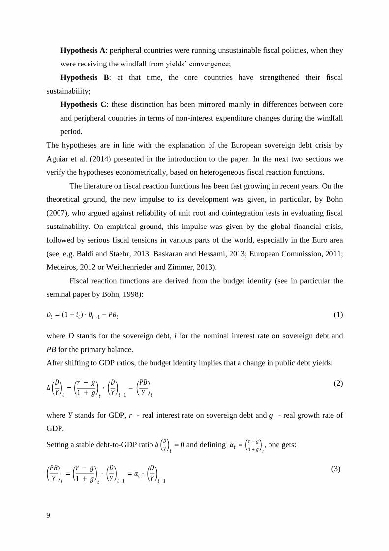
Fiscal reaction functions are derived from the budget identity (see in particular the

seminal paper by Bohn, 1998):

( ) (1)

where D stands for the sovereign debt, i for the nominal interest rate on sovereign debt and

PB for the primary balance.

After shifting to GDP ratios, the budget identity implies that a change in public debt yields:

(

) (

)

(

)

(

)

(2)

where Y stands for GDP, r - real interest rate on sovereign debt and g - real growth rate of

GDP.

Setting a stable debt-to-GDP ratio (

) and defining (

) , one gets:

(

) (

)

(

)

(

)

(3)

10

Equation (3) allows the estimation of the simplest fiscal reaction function:

(

)

(

)

(4)

Given that in a dynamically efficient economy, an inequality: > should hold16

, fiscal

sustainability requires a statistically significant and positive .

Empirical fiscal reaction functions usually include also output gap and government

expenditure gap to control for effects of cyclical fluctuations (see, e.g. Bohn, 1998), lag of

primary balance to allow for policy inertia (see, e.g. de Mello, 2005) or current account

balance to control for the “twin deficits” effect (Mendoza and Ostry , 2008 or European

Commission, 2011). In the first step of econometric analysis we start with the same

specification as European Commission (2011):

(5)

where is country effect, is the primary balance, is the sovereign debt, is

the output gap, is the cyclical component of government final consumption expenditure,

is the current account balance17

. We modify the specification in order to take into account

nonstationarity of the variables: according to Maddala and Wu (1999) and Pesaran (2007)

stationarity tests (results are presented in Table 1) only and vriables are

stationary18

. The final specification of fiscal reaction function (hereafter: Model 1) is

therefore:

(6)

*** Insert Table 1 here ***

We estimate equation (6) for 9 subsamples as specified in Table 2. As indicated in the

previous sections, the subsamples are created based on the scale of benefits from sovereign

16. At least in the long term, to which the notion of fiscal sustainability applies. Nevertheless, as already mentioned, Ball et al. (1998) provide some reservations to this claim with regard to sovereign bond yields.

17. Unlike Bohn (1998) and like European Commission (2011) and Mendoza and Ostry (2008) equation (5) does not include quadratic and

the cubic sovereign debt to control for possible non-linearity in the responsiveness of primary balance. It is worth noting that their inclusion in other studies gave results which are hardly robust. On the one hand, Bohn (1998) found that in the United States larger sovereign debt led

to stronger responsiveness of primary balance. IMF (2003), using debt-threshold dummies, confirms this result for industrialized countries.

Afonso (2008) finds an increasing responsiveness of primary balance to sovereign debt in the EU-15. On the other hand, the opposite effect is found by Calasun et al. (2007) and the IMF (2003) for the developing countries and by Ghosh et al. (2013) and Medeiros (2012) for the

industrialized economies and EU-15 respectively.

18. We are aware that the results of both tests may be biased. Maddala and Wu test assumes lack of cross-section dependence, which is actually the case for all analyzed variable but is most suitable for short and fixed time dimension as in our sample (Hoang and McNown,

2006). On the other hand, Pesaran test assumes cross-section dependence but T tending to infinity. Unfortunately, to our best knowledge

there is no test which addresses both of the shortcomings simultaneously.

11

bond yields’ convergence related to establishment of the Euro area. Given that these

definitions require some discretion, as part of robustness analysis, we re-estimate the model

under alternative composition of both groups of countries, and different splits of the analysed

period (for more on the robustness analysis, see section five).


In order to verify Hypotheses A and B, we compare lagged debt estimates

( ) between windfall and baseline period for peripheral and core countries. If the estimate

for peripheral countries, based on windfall subsample, is statistically non-significant or

significantly lower than the same parameter for baseline subsample, it will support

Hypothesis A. By the same token for core countries, statistically significant positive for

windfall subsample higher than baseline subsample would support Hypothesis B.

In the second step we estimate responsiveness of major categories of government

revenue and expenditure to changes in sovereign debt. Recall that as indicated in Hypothesis

C the divergence in fiscal sustainability between peripheral and core countries was mostly

driven by different paths of government non-interest spending. We estimate separate fiscal

reaction functions for (a) direct tax revenue ( ), (b) indirect tax revenue ( ), (c)

investment expenditure ( ) and (d) non-investment expenditure ( )19

. For each of

the variables we use specification presented in (6) e.g.

(7)

and each equation (hereafter: Model 2 - 5, respectively) has been estimated for 9 subsamples,

which gives us 36 estimates of . Direct comparison of values for different subsamples

and revenue or expenditure categories allows us to verify Hypothesis C.

Definitions of all variables used in the estimates and their data sources are presented in

Table 3. The majority of data are sourced from the AMECO database. Data on primary

balance for Ireland and Spain is obtained from the IMF WEO and the data on sovereign bond

yields – from the Eurostat. Descriptive statistics follow in Table 4.



19. This part of econometric analysis follows Favero and Marcellino (2005) and Burger and Marinkov (2012). The former paper uses the

fiscal reaction function framework for the government revenue and expenditure, while the latter applies it to specific categories of taxes and government expenditure.

12

We estimate the above equations using a set of panel data estimators. We begin with

fixed effects (FE) and random effects (RE) estimators, which assumes homogeneous

coefficients of the explanatory variables but allow for a different constant term for particular

countries. The results, based on the estimators mentioned, may be biased due to several

methodological problems. The first one is a possible cross-section dependence (or spatial

correlation) of error terms. In the analyzed model, this is equivalent to the assumption that

there are unobserved time-varying omitted variables common for all countries, which impact

individual states. Actually, the results of the Pesaran’s test for cross-section dependence

indicate that this is a characteristic of the data set used (but not necessarily of particular

subsamples). If these unobservable common factors are uncorrelated with the independent

variables, the coefficient estimates based on FE and RE regression are consistent, but standard

errors estimates are biased. Therefore, we use the Driscoll and Kraay (1998) nonparametric

covariance matrix estimator (DK) which corrects for the error structure spatial dependence.

This estimator also addresses the second problem, namely standard errors bias due to potential

heteroskedasticity and autocorrelation of the error terms. The third problem results from the

fact that the estimated equations are dynamic, so standard panel data estimators, such as fixed

effects (FE) and random effects (RE) are biased. One approach to addressing this problem is

to apply an instrumental variable estimator, such as that proposed by Arellano and Bond

(1991) or Arellano and Bover (1995). These estimators are asymptotically consistent, but their

properties are unsatisfactory in the case of short samples. As Kiviet (1995) notes, it is possible

to correct the bias of the standard estimators without affecting their efficiency. In this article,

we apply a corrected least square dummy variable estimator (LSDVC) proposed by Bun and

Kiviet (2002) and modified for the analysis of the unbalanced panels by Bruno (2005).

Taking into account all of the above restrictions, we use four types of panel data

estimators: fixed effects (FE), random effects (RE), Driscoll-Kraay (DK) and corrected least

square dummy variable estimator (LSDVC). That said, we are fully aware that our results

ought to be viewed with caution – at the very least due to estimation problems typical for

panel datasets with as short time dimension as in some of our subsamples.

IV. ESTIMATION RESULTS

We start the econometric analysis with verification of Hypotheses A and B put forward in

section three, on the basis of the theoretical model by Aguiar et al. (2014). To this aim we

13

estimate Model 1 for each of nine subsamples defined in Table 2 using four different

estimators. Table 5 provides results for the whole EU-12 sample with estimators and time

periods grouped in the particular columns. These models cover the largest data panel with up

to 402 observations, however they also conceal any heterogeneity within the EU-12. Lagged

public debt coefficients for all periods and estimators are positive and statistically significant

indicating that governments area-wide reduce fiscal deficits when faced with increases in debt

levels. In FE, DK and LSDVC estimators, reaction appears actually stronger during the

windfall period than the baseline. As the core country group dominates the EU-12 sample,

this may be attributed to its’ fiscal consolidations during the pre-accession period, which were

indicated by descriptive investigation in section three.


Tables 6 and Tables 7 show estimates for core and peripheral country groups respectively.

Results yield the primary support for Hypotheses A and B:

1. Estimates of ∆debtt-1 are positive and statistically significant in all cases except for the

windfall period in the peripheral country group, where it loses statistical significance

for the FE, RE and LSDVC estimators20

. It thus appears, that fiscal policy in

peripheral countries ceases to react to changes in sovereign debt during the windfall

years in accordance with Hypothesis A.

2. As further indicated by the coefficients of the ∆debtt-1 variable, fiscal positions of the

core member states react much more strongly to the levels of debt in the windfall

period than the baseline, with respective coefficients, amounted to 0.260-0.438 for the

former and 0.132-0.138 for the latter period (depending on the estimator used). The

results support Hypothesis B, which indicates that during windfall period core

countries, as opposed to peripheral ones, have strengthened their fiscal sustainability.

The result, which demands further elaboration, is the stronger reaction of fiscal balance to

sovereign debt in peripheral than core countries during the baseline period (estimates of

0.172-0.178 compared to 0.132-0.138). We see two plausible and non-exclusive explanations

for such results. First, the European sovereign debt crisis is part of the baseline period. This

may be unfortunate, but we cannot afford to leave it out, considering the limited size of our

sample. The peripheral member states, due to their dire fiscal positions, were required to

conduct stronger fiscal consolidations during this period than the core countries. Second,

20. 5% significance of the estimate obtained using DK estimator for windfall period in peripheral countries is rather spurious: the results of

Pesaran’s and Frees’ tests shown in the table indicate cross-section independence in this particular subsample. Utilizing the DK estimator in this case may yield biased estimates, as the ideas of the estimator is to correct standard errors for the presence of cross-section dependence.

14

Afonso (2008) found stronger responsiveness of fiscal policy at higher debt levels in the EU-

15 data during the 1970-2003 period. Mean consolidated gross debt in our sample is greater

for the periphery than core country group in every single year, perhaps explaining the

different responsiveness during the baseline period.



In the next step we estimate Model 2 – Model 5, i.e. fiscal reaction functions for tax

and spending categories, which allow to verify Hypothesis C. Results are presented in Table

8 in panels A-D respectively.21


First, in panel A (Model 2), we estimate a reaction function for direct taxes. Results

indicate that direct taxes were an adjustment instrument only during the baseline period in the

peripheral countries, which responded with tax increases to higher debt levels. In the

remaining subsamples the estimates are not significant.

Second, in panel B (Model 3), the reaction function is based on indirect taxes. In general,

it appears that peripheral countries have been increasing the indirect taxes in response to

rising debt in both periods, with stronger and more statistically significant estimates for the

windfall years. In the core member states rising debt coincided with opposite response in

indirect taxes, however the estimates are statistically significant only for the whole sample.

Third, in panel C (Model 4), an expenditure reaction function with investment expenditure

is estimated. It follows from results that both, core and periphery groups, used investment

spending as an adjustment mechanism to changing debt levels during the baseline timespan.

The adjustment has been significantly stronger for the periphery than core group (estimates of

-0.28 and -0.22 respectively). Both groups of countries did not use investment expenditure to

adjust to debt level during windfall years.

Fourth, in panel D (Model 5), non-investment expenditure reaction function is estimated.

In this case, results signal that non-investment expenditure has been an adjustment

mechanism in the baseline period for both core and peripheral member states, with stronger

and more statistically significant results for the core group. However, during the windfall

21. For the sake of brevity we restrict presentation of the results to lagged debt estimates only. Remaining estimates are available upon request.

15

timespan, results indicate even more substantial changes in reaction to debt fluctuations than

during baseline years in the core group, while lack of statistically significant relationship for

peripheral countries.

Recoupling the results give strong support to Hypothesis C:

1. During the baseline period, peripheral countries reacted to rising levels of debt

with cuts in both non-investment and investment expenditure. However, in the

windfall years, the fiscal stances of the peripheral member states ceased to react to

growing debt with expenditure cuts and increases in direct taxes, but instead

moved to rise the indirect taxes. As tax-based fiscal consolidations are typically

less likely to reduce debt-to-GDP ratios (Alesina and Ardagna, 2013), our results

give further credence to Hypothesis A.

2. The core member states in the baseline years responded to deteriorations in fiscal

position with non-investment spending cuts and much smaller decreases in

investment expenditure. In the windfall period, the core countries moved to

strengthen their fiscal stances with much stronger non-investment expenditure

consolidations than during the baseline period. This finding lends also further

support for Hypothesis B.

V. ROBUSTNESS ANALYSIS

In this section we examine if the results are robust to various changes in modelling approach.

All regressions presented in this section are carried out with fixed effects estimator, as

previously there were no major differences between the various estimation methods22

.

In part I and II of the analysis we check if the results are sensitive to the way, in which

cyclical factors are controlled for in the model. To this end, in Model 1 primary balance is

exchanged for the cyclically adjusted primary balance as the dependent variable and lagged

explanatory variable, while output gap is removed from explanatory variables. In part I, we

utilize the cyclically adjusted primary balance based on trend GDP23

and show results in

Table 9. As in our primary results, the ∆debtt-1 coefficient is positive and statistically

significant across all timespans and country groups, except for the windfall period in the

peripheral member states, where it lacks statistical significance. The strength of

responsiveness is similar to previous results. Subsequently, in part II, we utilize the cyclically

22. Results for other estimators are available on demand and they do not change our conclusions. 23. Trend GDP is calculated using the Hodrick-Prescott filter (European Commission, 2014; European Commission, 2000).

16

adjusted primary balance based on potential GDP24

instead of trend GDP. Results are

presented in Table 10. As previously, the ∆debtt-1 coefficient is positive and significant,

except the periphery sample during the windfall period.


*** Insert Table10 here ***

In part III we check whether our results are robust to excluding any single country

from our sample. Debt coefficients with their standard errors and significance levels from this

procedure are summarized in Table 11. Results for other estimators are available on demand

and they do not change our conclusions. When Belgium or Finland are excluded from the core

sample, statistical significance of fiscal responses during the baseline period is lost for the

core countries. However, the strength of the response remains similar and increased during

the windfall years and whole sample in the core country group. On the other hand, exclusion

of Greece from the periphery sample alters results in terms of both response strength and

statistical significance during all years and baseline periods in the periphery. There is not

much change in the all years EU-12 sample.


Subsequently, in part IV we alter the composition of the core and periphery groups.

The aim is to investigate the results when the periphery group is defined as the countries with

negative interest rate-growth differentials during the windfall period. This results in moving

Italy from the periphery to core country group. The outcome is presented in Table 12 and

does not alter our previous conclusions.


Finally, in part V we change the composition of baseline and windfall timespans. The

windfall period is now defined as pre-crisis Euro area membership years25

. Estimates are

presented in Table 13 and remain similar as previously, however the lagged debt coefficient

loses statistical significance during the baseline period in core countries. It is difficult to

account for this, nevertheless the result of a statistically insignificant response during the

24. Potential GDP is calculated based on a TFP adjusted Cobb-Douglas production function approach (European Commission, 2014; Denis

et al., 2002). 25. 2001-2007 for Greece and 1999-2007 for all other countries.

17

windfall period in the periphery remains valid (Hypothesis A) along with high fiscal policy

responsiveness in core countries during the windfall years (Hypothesis B).


In conclusion, the results are robust not only to the choice of different estimators (as

shown in the previous section), but also to the changes of the dependent variable (parts I and

II), exclusions of countries from the sample (part III), changes in country groups definitions

(part IV) and alternative time periods definitions (part V). Relatively small deviations are

present in the robustness analysis, however they are to be expected due to the small size of

our sample.

VI. DISCUSSION AND POLICY IMPLICATIONS

As mentioned in the introduction to the paper, studies analyzing fiscal sustainability in the

Euro area through the lens of fiscal reaction functions are hardly conclusive (cf. Baldi and

Staehr, 2013; Baskaran and Hessami, 2013; European Commission, 2011; Medeiros, 2012;

Weichenrieder and Zimmer, 2013). Our results are in line with these studies, which find

different reaction functions, for the pre-crisis period, in the peripheral countries, compared to

the core ones. We find the evidence that many similar studies fail to establish (see, e.g. Baldi

and Staehr, 2013 or Weichenrieder and Zimmer, 2013), possibly because we put stress on

windfall gained by the peripheral countries from the yields’ convergence, while these studies

usually focus either on establishment of the Euro area or on Euro adoption by peripheral

countries. It is worth noting that studies on fiscal reaction functions for Japan, which since

1990’s has been gaining a windfall of low interest burden due to unconventional monetary

policy measures, reach similar conclusions to ours (see, e.g. Doi et al., 2011; Ito et al., 2011;

Mauro et al., 2013 or Sakuragawa and Hosono, 2011).

Another main finding appears to be much less controversial. There is ample evidence that

the composition of fiscal adjustments matters for fiscal sustainability (see, e.g. Afonso et al.,

2005; Afonso and Jalles, 2012; Alesina and Ardagna, 2013, 2010 or 1998; Alesina and

Perotti, 1996; Alesina et al., 1998; Baldacci et al., 2010; von Hagen et al., 2002; von Hagen

and Strauch, 2001; Heylen et al., 2013; McDermott and Wescott, 1996; Purfield, 2003 or

Tsibouris et al., 2006). Our results suggest that this evidence also holds when one avoids

discretion in defining the notion of fiscal sustainability and instead refers to the budget

identity.

18

If these findings were correct, then they would have far reaching implications for

appropriate policy. They suggest that any actions which supress significance of country

specific credit risk in sovereign bonds’ prices, sow the seeds of a new crisis, given inherent

government’s temptation not to save a windfall of low interest burden. Paradoxically, the

more reason there is in the claims that the Euro area members are susceptible to similar risk to

the one faced by countries forced to issue debt in foreign currency (see, e.g. De Grauwe and

Ji, 2012a or 2012b), the greater the threat such actions cause. They widen the ranges of deficit

and debt levels, within which market does not act as a deterrent against unsustainable fiscal

policy. There is little chance that a government would not fully exploit this broader

opportunity to run unsustainable fiscal policy. The longer the market reactions are muted, the

more seriously the market may overreact (cf. Manganelli and Wolswijk, 2009). Our findings

would also contribute to the on-going debate on “austerity”26

. Namely, they suggest that the

peripheral countries have largely exhausted fiscal space during the pre-crisis period and have

had no choice but to struggle for restoring it thereafter. They suggest also that to make public

finances sustainable these countries should have adjusted mainly non-investment government

spending, rather than relied on tax increases or cuts in investment outlays.

VII. CONCLUDING REMARKS

We estimate various fiscal reaction functions for the 12 Euro area member states during the

1970-2013 period.

This allows us, firstly, to test two hypotheses which are implied by the explanation of the

European sovereign debt crisis provided by the theoretical model by Aguiar et al. (2014). We

find that the peripheral countries, in which sovereign bond yields fell deeply in the years

1996-2007, were running unsustainable fiscal policies. In contrast, in core countries which did

not benefit from yields’ convergence related to the Euro area establishment, fiscal

sustainability was strengthened during 1996-2007. These findings are robust to various

changes in modelling approach. They suggest that windfall gains are perilous not only for

developing countries but are likely to cause severe fiscal tensions even in advanced

economies.

Secondly, fiscal reaction functions that we estimate provide a new type of evidence that

the composition of fiscal innovations matters for fiscal sustainability. We find that

unsustainable fiscal policy in the peripheral countries during 1996-2007 resulted from lack of

26. It is surveyed, e.g. by Balcerowicz et al. (2013).

19

sufficient adjustment in government non-investment expenditure and direct taxes. In contrast,

the strengthened fiscal sustainability in the core countries at the time was mainly related to

pronounced adjustments of government non-investment expenditure.

We find our contributions both timely and policy relevant. That said, we are fully aware

that our results ought to be viewed with caution – at the very least due to estimation problems

typical for panel datasets with a short time dimension.

20

REFERENCES

Afonso, António (2008). Ricardian fiscal regimes in the European Union, Empirica.

35(3): 313-334.

Afonso, António and João T. Jalles (2011). Appraising fiscal reaction functions, ISEG

Department of Economics Working Papers No. 2011/23.

Afonso, António and João T. Jalles (2012). Measuring the success of fiscal consolidations,

Applied Financial Economics. 22(13): 1053-1061.

Afonso, António, Christiane Nickel and Philipp C. Rother (2005). Fiscal consolidations in

the Central and Eastern European countries, ECB Working Paper No. 473.

Afonso, António, Michael G. Arghyrou and Alexandros Kontonikas (2012). The

determinants of sovereign bond yield spreads in the EMU, ISEG Department of

Economics Working Papers No. 2012/36.

Afonso, António, Michael G. Arghyrou, George Bagdatoglou and Alexandros Kontonikas

(2013). On the time-varying relationship between EMU sovereign spreads and their

determinants, ISEG Department of Economics Working Papers No. 2013/05/DE/UECE.

Aguiar, Mark, Manuel Amador, Emmanuel Farhi and Gita Gopinath (2014).

Coordination and Crisis in Monetary Unions, NBER Working Paper No. 20277.

Alesina, Alberto F. and Roberto Perotti (1996). Fiscal Adjustments in OECD Countries:

Composition and Macroeconomic Effects, NBER Working Paper No. 5730.

Alesina, Alberto F. and Silvia Ardagna (1998). Tales of fiscal adjustment, Economic

Policy. 13(27): 487-546.

Alesina, Alberto F. and Silvia Ardagna (2010). Large changes in fiscal policy: taxes

versus spending, in: Jeffrey R. Brown (ed.), Tax Policy and the Economy. 24: 35-68,

Cambridge: University of Chicago Press.

Alesina, Alberto F. and Silvia Ardagna (2013). The Design of Fiscal Adjustments, in

Jeffrey R. Brown (ed.), Tax Policy and the Economy. 27: 19-67, Chicago: University of

Chicago Press.

Alesina, Alberto F., Roberto Perotti, and Jose Tavares (1998). The Political Economy of

Fiscal Adjustments, Brookings Papers on Economic Activity. 1: 197-266.

Arellano, Manuel and Olympia Bover (1995). Another Look at the Instrumental Variable

Estimation of Error-Components Models, Journal of Econometrics. 68(1): 29-51.

Arellano, Manuel and Stephen Bond (1991). Some Tests of Specification for Panel Data:

Monte Carlo Evidence and an Application to Employment Equations, Review of Economic

Studies. 58(2): 277-97.

Arghyrou, Michael G. and Alexandros Kontonikas (2012). The EMU sovereign-debt

crisis: Fundamentals, expectations and contagion, Journal of International Financial

Markets, Institutions and Money. 22(4): 658-677.

Aßmann, Christian and Jens Boysen-Hogrefe (2012). Determinants of government bond

spreads in the euro area: in good times as in bad, Empirica. 39(3): 341-356.

Attinasi, Maria-Grazia, Cristina Checherita and Christiane Nickel (2009). What explains

the surge in euro area sovereign spreads during the financial crisis of 2007-09?, ECB

Working Paper Series No. 1131.

Auerbach, Alan J. (2011). Fiscal Institutions for a Currency Union, Paper prepared for a

conference on Fiscal and Monetary Policy Challenges in the Short and Long Run,

sponsored by the Deutsche Bundesbank and the Banque de France, Hamburg, May 19-20.

Balcerowicz, Leszek, Andrzej Rzońca, Lech Kalina and Aleksander Łaszek (2013).

Economic Growth in the European Union. Brussels: Lisbon Council.

21

Baldacci, Emanuele, Sanjeev Gupta and Carlos Mulas-Granados (2010). Restoring Debt

Sustainability After Crises: Implications for the Fiscal Mix, IMF Working Paper No.

10/232.

Baldi, Guido and Karsten Staehr (2013). The European Debt Crisis and Fiscal Reaction

Functions in Europe 2000-2012, Discussion Papers of DIW Berlin No. 1295.

Ball, Laurence, Douglas W. Elmendorf and N. Gregory Mankiw (1998). The Deficit

Gamble, Journal of Money, Credit and Banking. 30(4): 699-720.

Barrios, Salvador, Per Iversen, Magdalena Lewandowska and Ralph Setzer (2009).

Determinants of intra-euro area government bond spreads during the financial crisis,

European Economy - Economic Papers No. 388.

Baskaran, Thushyanthan and Zohal Hessami (2013). Monetary Integration, Soft Budget

Constraints, and the EMU Sovereign Debt Crises, Working Paper Series of the

Department of Economics No. 2013-03. University of Konstanz.

Bernoth, Kerstin and Burcu Erdogan (2012). Sovereign bond yield spreads: A time-

varying coefficient approach, Journal of International Money and Finance. 31(3): 639-

656.

Bohn, Henning (1998). The Behavior of U.S. Public Debt and Deficits, The Quarterly

Journal of Economics. 113(3): 949-963.

Bohn, Henning (2007). Are Stationary and Cointegration Restrictions Really Necessary

for the Intertemporal Budget Constraint?, Journal of Monetary Economics. 57(7): 1837-

1847.

Borgy, Vladimir, Thomas Laubach, Jean-Stéphane Mésonnier and Jean-Paul Renne

(2012). Fiscal Sustainability, Default Risk and Euro Area Sovereign Bond Spreads

Markets, Banque de France Working papers No. 350.

Briotti, Maria G. (2004). Fiscal adjustment between 1991 and 2002 - stylised facts and

policy implications, ECB Occasional Paper Series No. 09.

Bronner, Fernando, Aitor Erce, Alberto Martin and Jaume Ventura (2014). Sovereign debt

markets in turbulent times: Creditor discrimination and crowding-out effects, Journal of

Monetary Economics. 61: 114-142.

Bruno, Giovanni S.F. (2005). Approximating the bias of the LSDV estimator for dynamic

unbalanced panel data models, Economics Letters. 87(3): 361-366.

Bun, Maurice and Jan F. Kiviet (2002). On the Diminishing Returns of Higher-order

Terms in Asymptotic Expansions of Bias, Tinbergen Institute Discussion Papers No. 02-

099/4.

Burger, Philippe and Marina Marinkov (2012). Fiscal rules and regime-dependent fiscal

reaction functions: The South African case, OECD Journal on Budgeting. 12(1).

Caballero, Ricardo J. (2010). Sudden Financial Arrest, IMF Economic Review. 58(1): 6-

36.

Caporale, Guglielmo M. and Alessandro Girardi (2011). Fiscal Spillovers in the Euro

Area, CESifo Working Paper Series No. 3693.

Celasun, Oya, Xavier Debrun and Jonathan D. Ostry (2007). Primary Surplus Behavior

and Risks to Fiscal Sustainability in Emerging Market Countries: A "Fan-Chart"

Approach, IMF Staff Papers, 53(3): 401-425.

Corsetti, Giancarlo, Keith Kuester, André Meier and Gernot J. Müller (2014). Sovereign

risk and belief-driven fluctuations in the euro area, Journal of Monetary Economics.

61(1): 53-73.

De Grauwe, Paul and Yuemei Ji (2012a). Mispricing of Sovereign Risk and Multiple

Equilibria in the Eurozone, CEPS Papers No. 6548.

22

De Grauwe, Paul and Yuemei Ji (2012b). Mispricing of Sovereign Risk and

Macroeconomic Stability in the Eurozone, JCMS: Journal of Common Market Studies.

50(6): 866–880.

de Mello, Luiz. (2005). Estimating a Fiscal Reaction Function: The Case of Debt

Sustainability in Brazil, OECD Economics Department Working Papers No. 423.

De Santis, Roberto A. (2012). The Euro area sovereign debt crisis: safe haven, credit

rating agencies and the spread of the fever from Greece, Ireland and Portugal, ECB

Working Paper Series No. 1419.

Denis, Cécile, Kieran McMorrow and Werner Röger (2002). Production function

approach to calculating potential growth and output gaps – estimates for the EU Member

States and the US, European Economy - Economic Papers No. 176.

Doi, Takero, Takeo Hoshi and Tatsuyoshi Okimoto (2011). Japanese government debt and

sustainability of fiscal policy, Journal of the Japanese and International Economies.

25(4): 414-433.

Driscoll, John C. and Aart Kraay (1998). Consistent Covariance Matrix Estimation With

Spatially Dependent Panel Data, The Review of Economics and Statistics. 80(4): 549-560.

European Commission (2000). European Economy Public finances in EMU – 2000,

European Economy – Reports and Studies No. 3, European Commission.

European Commission (2011). Public finances in EMU - 2011, European Economy No. 3.

European Commission (2014). Cyclical Adjustment of Budget Balances – Autumn 2014.

Favero, Carlo A. and Massimiliano Marcellino (2005). Modelling and Forecasting Fiscal

Variables for the Euro Area, Oxford Bulletin of Economics and Statistics. 67(S1): 755-

783.

Favero, Carlo and Tommaso Monacelli (2005). Fiscal Policy Rules and Regime

(In)Stability: Evidence from the U.S., IGIER Working Papers No. 282.

Fernández-Villaverde, Jesús, Luis Garicano and Tano Santos (2013). Political Credit

Cycles: the Case of the Euro Zone, Journal of Economic Perspectives. 27(3): 145-166.

Fischer, Stanley and William Easterly (1990). The economics of the government budget

constraint, World Bank Research Observer. 5(2): 127-142.

Frees, Edward W. (2004). Longitudinal and panel data: Analysis and Applications in the

Social Sciences. Cambridge: Cambridge University Press.

Gerlach, Stefan, Alexander Schulz and Guntram B. Wolff (2010). Banking and sovereign

risk in the euro-area, CEPR Discussion Paper No. 7833.

Ghosh, Atish R., Jun I. Kim, Enrique G. Mendoza, Jonathan D. Ostry and Mahvash S.

Qureshi (2013). Fiscal Fatigue, Fiscal Space and Debt Sustainability in Advanced

Economies, The Economic Journal. 123(566): F4–F30.

Gibson, Heather D., Stephen G. Hall and George S. Tavlas (2012). The Greek financial

crisis: Growing imbalances and sovereign spreads, Journal of International Money and

Finance. 31(3): 498-516.

Gros, Daniel (2013). The austerity debate is beside the point for Europe, CEPS

Commentaries. May 8.

Gylafson, Thorvaldur (2011). Natural Resource Endowment: A Mixed Blessing?, CESifo

Working Paper No. 3353.

Haugh, David, Patrice Ollivaud and David Turner (2009). What Drives Sovereign Risk

Premiums?: An Analysis of Recent Evidence from the Euro Area, OECD Economics

Department Working Papers No. 718.

Heylen, Freddy, Annelies Hoebeeck and Tim Buyse (2013). Government efficiency,

institutions, and the effects of fiscal consolidation on public debt, European Journal of

Political Economy. 31(C): 40-59.

23

Hoang, Nam T. and Robert F. McNown (2006). Panel Data Unit Roots Tests Using

Various Estimation Methods, working paper, Department of Economics, University of

Colorado at Boulder.

IMF (2003). Public Debt in Emerging Markets, World Economic Outlook. September:

113-152.

Ito, Arata, Tsutomu Watanabe and Tomoyoshi Yabu (2011). Fiscal Policy Switching in

Japan, the US, and the UK, Journal of the Japanese and International Economies. 25(4):

380-413.

Kang Joong S. and Jay Shambaugh (2014). Progress Towards External Adjustment in the

Euro Area Periphery and the Baltics, IMF Working Paper No. 14/131.

Kiviet, Jan F. (1995). On Bias, Inconsistency and Efficiency of Various Estimators in

Dynamic Panel Data Models, Journal of Econometrics. 68(1): 53-78.

Lane, Philip R. (2012). The European Sovereign Debt Crisis, Journal of Economic

Perspectives. 26(3): 49-68.

Laubach, Thomas (2011). Fiscal Policy and Interest Rates: The Role of Sovereign Default

Risk, in Richard Clarida and Francesco Giavazzi (eds.), NBER International Seminar on

Macroeconomics 2010. Chicago: University of Chicago Press: 7-29.

Maddala, G.S. Shaowen Wu (1999). A comparative study of unit root tests with panel data

and a new simple test, Oxford Bulletin of Economics and Statistics. 61(S1): 631–652.

Manganelli, Simone and Guido Wolswijk (2009). What drives spreads in the euro area

government bond market?, Economic Policy. 24(58): 191-240.

Mauro, Paolo, Rafael Romeu, Ariel Binder and Asad Zaman (2013). A Modern History of

Fiscal Prudence and Profligacy, IMF Working Paper No. 13/5.

McDermott, C. John and Robert F. Westcott (1996). An Empirical Analysis of Fiscal

Adjustments, IMF Staff Papers. 43(4): 723-753.

Medeiros, João (2012). Stochastic debt simulation using VAR models and a panel fiscal

reaction function – results for a selected number of countries, European Economy -

Economic Papers No. 459.

Mehlum, Halvor, Karl Moene and Ragnar Torvik (2006). Cursed by Resources or

Institutions?, World Economy. 29(8): 1117-1131.

Mendoza, Enrique G. and Jonathan D. Ostry (2008). International evidence on fiscal

solvency: Is fiscal policy 'responsible'?, Journal of Monetary Economics. 55(6): 1081-

1093.

Pesaran, M. Hashem (2007). A Simple Panel Unit Root Test in the Presence of Cross-

Section Dependence, Journal of Applied Econometrics. 22(2): 265-312.

Purfield, Catriona (2003). Fiscal Adjustment in Transition Countries: Evidence from the

1990s, IMF Working Paper No. 03/36.

Sakuragawa, Masaya and Kaoru Hosono (2011). Fiscal Sustainability in Japan, Journal of

Japanese and International Economies. 25(4): 434-446.

Shambaugh, Jay C. (2012). The Euro’s Three Crises, Brookings Papers on Economic

Activity. 44(1): 157-231.

Steikamp, Sven and Frank Westermann (2014). The role of creditor seniority in Europe’s

sovereign debt crisis, Economic Policy. 29(79): 495-552.

Svensson, Jakob (2000). Foreign Aid and Rent-Seeking, Journal of International

Economics. 51(2): 437–461.

Tsibouris, George C., Mark A. Horton, Mark J. Flanagan and Wojciech S. Maliszewski

(2006). Experience with Large Fiscal Adjustments, IMF Occasional Paper No. 246.

Vamvakidis, Athanasios (2007). External Debt and Economic Reform: Does a Pain

Reliever Delay the Necessary Treatment, IMF Working Paper No. 07/50.

24

von Hagen, Jurgen and Rolf Strauch (2001). Fiscal Consolidations: Quality, Economic

Conditions, and Success, Public Choice. 109(3-4): 327-46.

von Hagen, Jurgen, Andrew Hughes-Hallett and Rolf Strauch (2002). Budgetary

Consolidation in Europe: Quality, Economic Conditions, and Persistence. Journal of the

Japanese and International Economies. 16(4): 512-535.

von Hagen, Jurgen, Ludger Schuknecht and Guido Wolswijk (2011). Government bond

risk premiums in the EU revisited: The impact of the financial crisis, European Journal of

Political Economy. 27(1): 36-43.

Weichenrieder, Alfons J. and Jochen Zimmer (2013). Euro Membership and Fiscal

Reaction Functions, CESifo Working Paper Series No. 4255.

25

APPENDIX

FIGURE 1. Government bond spreads against Germany (percentage points)

Note: German long-term government bond yields have been subtracted from values for every single country (including

Germany) and then averaged. Further information on the source and computation method are given in Table 3.

FIGURE 2. Interest rate-growth differential (percentage points)

Note: Interest rate growth differential is defined as the differential between the cost of debt and growth rate of nominal GDP.

Effective interest rate on sovereign debt is approximated by the ratio of government interest payments to sovereign debt. The

same approximation is used, e.g. by Favero and Monacelli (2005). Further information on the source and computation

method are given in Table 3.

26

FIGURE 3. Change in main fiscal categories. EU-12 core and peripherial countries from 1996 to 1999 (percentage points

of GDP)

Note: 1996 values have been subtracted from 1999. All variables are cyclically adjusted based on potential GDP.

Appraisal of fiscal policy in the EU-12 core and periphery does not change when analysis is based on values cyclically

adjusted with trend GDP or without any cyclical adjustment.

FIGURE 4. Change in main fiscal categories. EU-12 core and peripherial countries from 1999 to 2007 (percentage points

of GDP)

Note: 1999 values have been subtracted from 2007. All variables are cyclically adjusted based on potential GDP.

Appraisal of fiscal policy in the EU-12 core and periphery does not change when analysis is based on values cyclically

adjusted with trend GDP or without any cyclical adjustment.

27

TABLE 1. Panel unit root tests

Variables

Test

Levels/first

differences Trend Lags pbalance debt ogap ggap cab dirtax indtax invexp consexp capb_p capb_t

Mad

dala an

d W

u 1

999

Levels No 0 59.921*** 59.922 59.923*** 59.924*** 59.925* 59.93*** 59.931 59.928* 59.929* 59.926*** 59.927***

Levels No 1 65.777*** 13.37 122.474*** 238.083*** 40.287** 51.167*** 50.148*** 38.875** 37.148** 56.211*** 48.528***

Levels No 2 44.054*** 16.209 80.265*** 152.563*** 36.782** 41.184** 37.676** 28.354 26.586 37.199** 33.115

Levels No 3 37.749** 20.535 88.567*** 136.497*** 32.39 32.524 31.759 21.196 31.281 33.535* 34.464*

Levels Yes 0 41.555** 4.701 52.117*** 98.104*** 30.297 40.368** 29.155 26.751 30.123 51.964*** 42.279**

Levels Yes 1 49.048*** 25.6 96.433*** 181.411*** 40.257** 47.951*** 45.909*** 24.51 43.655*** 43.509*** 35.698*

Levels Yes 2 31.906 22.097 57.482*** 106.593*** 46.461*** 44.174*** 32.092 11.463 24.527 28.828 25.27

Levels Yes 3 27.608 29.546 65.579*** 94.899*** 41.744** 30.386 36.064* 10.133 26.652 24.103 23.475

Dif. No 0 366.968*** 142.495*** 366.065*** 406.849*** 443.984*** 320.868*** 326.985*** 329.609*** 316.286*** 430.71*** 413.737***

Dif. No 1 234.341*** 96.154*** 323.642*** 393.783*** 233.938*** 182.921*** 208.067*** 214.295*** 196.024*** 235.124*** 213.741***

Dif. No 2 149.736*** 68.287*** 198.492*** 290.253*** 145.134*** 135.126*** 143.485*** 129.157*** 127.054*** 147.906*** 130.172***

Dif. No 3 106.919*** 66.546*** 196.633*** 219.695*** 152.133*** 108.106*** 122.929*** 89.3*** 83.483*** 97.506*** 82.099***

Dif. Yes 0 306.723*** 126.428*** 301.847*** 333.403*** 377.686*** 258.77*** 274.634*** 281.44*** 262.52*** 354.767*** 341.076***

Dif. Yes 1 190.585*** 72.525*** 261.715*** 322.512*** 189.42*** 133.273*** 167.65*** 180.794*** 154.237*** 179.872*** 160.69***

Dif. Yes 2 116.551*** 51.05*** 148.548*** 228.114*** 110.224*** 91.043*** 109.89*** 104.227*** 103.558*** 108.147*** 92.256***

Dif. Yes 3 83.811*** 51.692*** 156.09*** 162.463*** 111.482*** 71.532*** 90.938*** 72.309*** 70.117*** 69.912*** 55.038***

Pesaran

(200

7)

Levels No 0 -3.087*** 3.449 -4.275*** -6.837*** -0.385 -2.496*** -1.162 -0.67 -0.581 -3.748*** -3.345***

Levels No 1 -2.322** 1.321 -4.342*** -7.279*** -0.501 -1.825** -1.169 0.13 0.348 -2.334** -2.221**

Levels No 2 -1.382* 0.865 -2.676*** -6.241*** -0.006 0.078 -0.202 0.917 1.502 -0.966 -0.601

Levels No 3 -0.645 0.44 -2.785*** -4.673*** 0.303 -0.285 -0.467 1.351 1.764 -0.525 -0.311

Levels Yes 0 -2.102** 6.128 -3.057*** -4.883*** 0.364 -2.151** -0.501 0.232 -0.049 -3.079*** -2.704***

Levels Yes 1 -0.868 3.204 -3.202*** -5.364*** -0.132 -1.992** -0.804 1.577 1.122 -0.907 -0.602

Levels Yes 2 0.016 3.642 -1.515* -4.345*** -0.326 -0.583 0.744 2.459 1.659 0.681 1.279

Levels Yes 3 0.042 4.015 -1.895** -2.435*** 0.104 -1.171 0.749 3.041 1.358 1.01 1.515

Dif. No 0 -13.352*** -8.722*** -13.624*** -14.336*** -14.917*** -13.388*** -13.252*** -12.679*** -13.302*** -14.147*** -13.903***

Dif. No 1 -9.263*** -4.037*** -11.648*** -11.788*** -10.16*** -9.022*** -9.676*** -7.088*** -7.66*** -10.012*** -9.945***

Dif. No 2 -5.831*** -1.908** -8.004*** -8.747*** -6.588*** -5.983*** -5.292*** -3.786*** -4.017*** -5.633*** -5.477***

Dif. No 3 -3.113*** -0.879 -8.162*** -7.659*** -4.826*** -4.801*** -3.695*** -1.355* -1.633* -2.914*** -2.481***

Dif. Yes 0 -12.672*** -8.056*** -12.788*** -13.297*** -14.119*** -12.101*** -12.123*** -11.549*** -13.166*** -13.071*** -12.906***

Dif. Yes 1 -8.547*** -3.704*** -10.198*** -10.251*** -8.703*** -7.245*** -8.255*** -5.719*** -6.418*** -8.344*** -8.131***

Dif. Yes 2 -5.021*** -1.595* -6.431*** -6.866*** -5.012*** -4.378*** -3.661*** -2.425*** -2.891*** -4.095*** -3.753***

Dif. Yes 3 -2.064** -1.111 -7.182*** -5.596*** -3.066*** -3.523*** -1.418* 0.096 -0.86 -1.496* -1.003

Notes: The first test is Maddala and Wu (1999) panel unit root test. Results shown are chi-square statistics. The second test is a Pesaran (2007) Panel Unit Root Test (CIPS). Results are Zt-bars.

Stars denote stationarity at 1% (***), 5% (**), 10% (*) levels.

28

TABLE 2. Number of observations by country group and period

Group of countries All years

1970-2013

Baseline

1970-1995 & 2008-2013

Windfall

1996-2007

Core (Austria, Belgium, Finland, France, Germany, Luxembourg, Netherlands)

250 166 84

Periphery (Greece, Ireland, Italy, Portugal, Spain)

152 92 60

EU-12 (all of the above)

402 258 144

29

TABLE 3. Variable definitions

Variable Name in

models Unit Definition Source

Primary balance pbalance % GDP Primary balance of general government. Note that data is sourced from AMECO, however gaps

for Ireland (1980-1984) and Spain (1980-1994) are completed with WEO data. EC AMECO, IMF WEO

Debt debt % GDP Consolidated gross debt of general government. EC AMECO

Output gap ogap % GDP Gap between actual GDP and potential GDP. EC AMECO

Cyclical component of government final

consumption expenditure ggap % GDP

Cyclical component of final consumption expenditure of general government, constructed by

detrending the final government consumption expenditure as a share of GDP with the Hodrick-

Prescott filter (smoothing parameter set at 100).

Authors' calculations

based on EC AMECO

Current account balance cab % GDP Current account balance. EC AMECO

Cyclically adjusted primary balance

(trend GDP) capb_p % GDP Cyclically adjusted primary balance based on potential GDP. EC AMECO

Cyclically adjusted primary balance

(potential GDP) capb_t % GDP Cyclically adjusted primary balance based on trend GDP. EC AMECO

Indirect taxes indtax % GDP Taxes linked to imports and production. EC AMECO

Direct taxes dirtax % GDP Current taxes on income and wealth. EC AMECO

Investment expenditure invexp % GDP Gross fixed capital formation of general government. EC AMECO

Non-investment expenditure consexp % GDP Total expenditure of general government excluding interest and gross fixed capital formation. Authors' calculations

based on EC AMECO

Cyclically adjusted budget balance NA % GDP Cyclically adjusted budget balance of general government based on potential GDP. EC AMECO

Cyclically adjusted revenue NA % GDP Cyclically adjusted revenue of general government based on potential GDP. EC AMECO

Cyclically adjusted non-interest

expenditure NA % GDP Cyclically adjusted non-interest expenditure of general government based on potential GDP. EC AMECO

Cyclically adjusted interest payments NA % GDP Cyclically adjusted interest payments of general government based on potential GDP. Authors' calculations

based on EC AMECO

Interest-rate-growth differential NA Percentage

points

Differential between the cost of debt (computed by dividing interest payments in ECU/EUR by

consolidated gross debt of general government in ECU/EUR) and growth rate of nominal GDP.


based on EC AMECO

Bond spreads against Germany NA Percentage

points

Long-term government bond spreads against Germany based on EMU convergence criterion

bond yields. German bond yields have been subtracted from values for every single country

(including Germany) and then averaged. Yearly values have been aggregated from monthly

data.


based on Eurostat

30

TABLE 4. Descriptive statistics

All years Baseline Windfall

1970-2013 1970-1995 & 2008-2013 1996-2007

Name in

models Unit Obs Mean SD Min Max Obs Mean SD Min Max Obs Mean SD Min Max

Primary balance pbalance % GDP 433 0.55 3.19 -11.6 9.81 289 -0.29 3.16 -11.64 8.33 144 2.25 2.50 -3.97 9.81

Debt debt % GDP 513 56.51 33.76 4.05 175.05 369 53.73 34.95 4.05 175.05 144 63.65 29.43 6.07 127.15

Output gap ogap % potential

GDP 515 -0.01 2.51 -12.58 8.13 371 -0.35 2.69 -12.58 8.13 144 0.87 1.70 -3.57 5.61

Cyclical component of

government final

consumption expenditure

ggap % GDP 528 -0.00 0.63 -2.27 2.52 384 0.06 0.66 -2.27 2.52 144 -0.16 0.52 -1.50 1.51

Current account balance cab % GDP 528 0.27 5.77 -17.96 25.09 384 0.14 5.63 -17. 25.09 144 0.61 6.15 -17.63 13.22

Cyclically adjusted

primary balance

(potential GDP)

capb_p % GDP 414 0.67 3.16 -25.41 9.05 270 0.04 3.33 -25.41 9.05 144 1.86 2.42 -3.68 8.79

Cyclically adjusted

primary balance (trend

GDP)

capb_t % GDP 414 0.57 3.40 -25.12 8.61 270 -0.14 3.54 -25.12 8.43 144 1.91 2.66 -6.69 8.61

Indirect taxes indtax % GDP 414 12.61 1.78 7.68 15.94 270 12.40 1.91 7.68 15.94 144 13.01 1.42 9.91 15.89

Direct taxes dirtax % GDP 414 12.40 3.17 4.53 21.09 270 12.24 3.25 4.53 18.83 144 12.69 3.01 6.40 21.09

Investment expenditure invexp % GDP 414 3.05 0.91 1.00 5.46 270 3.13 0.88 1.00 5.46 144 2.88 0.95 1.07 5.26

Non-investment

expenditure consexp % GDP 414 40.64 6.28 24.37 58.93 270 41.28 6.46 24.37 58.93 144 39.45 5.75 25.68 53.15

31

TABLE 5. Estimation results. Fiscal reaction function, EU-12, dependent variable: primary balance

FE RE DK LSDVC

1970-2013

1970-1995

&

2008-2013

1996-2007 1970-2013

1970-1995

&

2008-2013

1996-2007 1970-2013

1970-1995

&

2008-2013

1996-2007 1970-2013

1970-1995

&

2008-2013

1996-2007

All years Baseline Windfall All years Baseline Windfall All years Baseline Windfall All years Baseline Windfall

∆pbalancet-1 -0.163** -0.125 -0.251*** -0.161** -0.111 -0.239*** -0.163** -0.125* -0.251 -0.139*** -0.088 -0.186**

(0.069) (0.074) (0.059) (0.070) (0.079) (0.065) (0.060) (0.058) (0.151) (0.042) (0.062) (0.085)

∆debtt-1 0.143*** 0.157*** 0.216* 0.138*** 0.158*** 0.157** 0.143*** 0.157*** 0.216*** 0.143*** 0.158*** 0.213***

(0.027) (0.041) (0.105) (0.024) (0.038) (0.069) (0.024) (0.024) (0.057) (0.029) (0.051) (0.050)

ogapt 0.072 0.113* -0.070 0.080 0.131** -0.155** 0.072 0.113* -0.070 0.070* 0.111 -0.074

(0.060) (0.062) (0.084) (0.059) (0.059) (0.060) (0.059) (0.056) (0.118) (0.041) (0.109) (0.101)

ggapt -1.604*** -1.651*** -1.408*** -1.576*** -1.599*** -1.537*** -1.604*** -1.651*** -1.408*** -1.590*** -1.627*** -1.398***

(0.159) (0.158) (0.345) (0.162) (0.162) (0.350) (0.406) (0.488) (0.279) (0.157) (0.248) (0.264)

∆cabt -0.018 0.004 -0.050 -0.008 0.014 0.001 -0.018 0.004 -0.050 -0.017 0.004 -0.051

(0.070) (0.092) (0.074) (0.066) (0.094) (0.060) (0.059) (0.064) (0.111) (0.058) (0.073) (0.094)

constant -0.225*** -0.365*** 0.234*** -0.216*** -0.361*** 0.244** -0.225 -0.365 0.234 NA NA NA

(0.032) (0.096) (0.051) (0.064) (0.137) (0.110) (0.194) (0.219) (0.374)

N 402 258 144 402 258 144 402 258 144 402 258 132

Within R2 0.2807 0.3394 0.2239 0.2805 0.3390 0.2127 0.2807 0.3394 0.2239 NA NA NA

Between R2 0.0267 0.2636 0.0520 0.0308 0.2890 0.2302 NA NA NA NA NA NA

Overall R2 0.2755 0.3373 0.1963 0.2757 0.3378 0.2105 NA NA NA NA NA NA

Pesaran's test (p-

val) 0.0000 0.0000 0.0000 0.0000 0.0000 0.0000 NA NA NA NA NA NA

Frees' test

(statistic) 1.397*** 1.102*** 1.194*** 1.455*** 1.047*** 1.206*** NA NA NA NA NA NA

Breush-Pagan's

test (p-val) NA NA NA 1.0000 1.0000 1.0000 NA NA NA NA NA NA

Notes: The dependent variable is primary balance and the estimated model is given by ∆pbalanceit = αi + α1∙∆pbalanceit-1 + α2∙∆debtit-1 + α3∙ogapit + α4∙ggapit + α5∙∆cabit + εit. Core consists of

Austria, Belgium, Finland, France, Germany, Luxembourg and the Netherlands. Periphery encompasses Greece, Ireland, Italy, Portugal and Spain. EU-12 is the sum of core and periphery.

Variables definitions are reported in Table 3. The first row of the table lists the estimators used in the subsequent regressions, while the second row indicates time dimension of the sample. We

use four types of panel data estimators: fixed effects (FE), random effects (RE), Driscoll–Kraay with corrected standard errors (DK) and a bias-corrected least squares dummy variables

(LSDVC). For Breush-Pagan’s and Pesaran’s (2004) cross-section dependence test results shown are p-values. For Frees’ (2004) cross-section dependence test results shown are Q-statistics.

Standard errors are given in parentheses. Stars denote estimates significance at 1% (***), 5% (**), 10% (*) levels.

32

TABLE 6. Estimation results. Fiscal reaction function, EU-12 core, dependent variable: primary balance

FE RE DK LSDVC

1970-2013

1970-1995

&

2008-2013

1996-2007 1970-2013

1970-1995

&

2008-2013

1996-2007 1970-2013

1970-1995

&

2008-2013

1996-2007 1970-2013

1970-1995

&

2008-2013

1996-2007


∆pbalancet-1 -0.217** -0.178** -0.216** -0.214*** -0.161** -0.244*** -0.217** -0.178* -0.216 -0.195*** -0.147* -0.157

(0.078) (0.071) (0.062) (0.079) (0.076) (0.076) (0.087) (0.085) (0.138) (0.052) (0.086) (0.101)

∆debtt-1 0.121*** 0.132** 0.438** 0.120*** 0.138*** 0.260*** 0.121** 0.132** 0.438*** 0.121*** 0.135*** 0.428***

(0.032) (0.049) (0.136) (0.031) (0.049) (0.092) (0.037) (0.041) (0.112) (0.036) (0.050) (0.097)

ogapt -0.025 -0.024 0.023 -0.013 0.014 -0.103 -0.025 -0.024 0.023 -0.027 -0.026 0.022

(0.052) (0.081) (0.105) (0.057) (0.074) (0.106) (0.067) (0.069) (0.111) (0.068) (0.078) (0.149)

ggapt -1.922*** -2.038*** -1.652*** -1.890*** -1.968*** -1.750*** -1.922*** -2.038*** -1.652*** -1.908*** -2.022*** -1.620***

(0.149) (0.215) (0.394) (0.144) (0.198) (0.440) (0.301) (0.376) (0.421) (0.256) (0.312) (0.557)

∆cabt 0.058 0.106 -0.083 0.061 0.113 -0.052 0.058 0.106 -0.083 0.061 0.109 -0.085

(0.057) (0.099) (0.126) (0.059) (0.098) (0.116) (0.086) (0.104) (0.119) (0.077) (0.119) (0.131)

constant -0.181*** -0.396*** 0.472*** -0.180*** -0.397*** 0.408*** -0.181 -0.396* 0.472 NA NA NA

(0.037) (0.101) (0.058) (0.064) (0.152) (0.123) (0.209) (0.169) (0.461)

N 250 166 84 250 166 84 250 166 84 250 166 77

Within R2 0.2775 0.3555 0.2842 0.2774 0.3546 0.2592 0.2775 0.3555 0.2842 NA NA NA



Pesaran's test (p-


Frees' test

(statistic) 1.222*** 0.804*** 1.162*** 1.251*** 0.737*** 1.470*** NA NA NA NA NA NA

Breush-Pagan's








33

TABLE 7. Estimation results. Fiscal reaction function, EU-12 periphery, dependent variable: primary balance

FE RE DK LSDVC

1970-2013

1970-1995

&

2008-2013

1996-2007 1970-2013

1970-1995

&

2008-2013

1996-2007 1970-2013

1970-1995

&

2008-2013

1996-2007 1970-2013

1970-1995

&

2008-2013

1996-2007


∆pbalancet-1 -0.089 -0.076 -0.273*** -0.084 -0.064 -0.220*** -0.089 -0.076 -0.273 -0.054 -0.016 -0.184*

(0.132) (0.165) (0.059) (0.134) (0.172) (0.053) (0.084) (0.105) (0.150) (0.090) (0.160) (0.096)

∆debtt-1 0.164** 0.177** 0.106 0.155*** 0.172*** 0.083 0.164*** 0.177*** 0.106** 0.163*** 0.178** 0.106

(0.042) (0.060) (0.088) (0.040) (0.058) (0.075) (0.025) (0.030) (0.037) (0.035) (0.069) (0.066)

ogapt 0.100 0.146 -0.195 0.106 0.161** -0.208 0.100 0.146* -0.195 0.098 0.141 -0.194

(0.082) (0.086) (0.165) (0.083) (0.081) (0.155) (0.065) (0.062) (0.106) (0.065) (0.154) (0.149)

ggapt -1.404*** -1.513*** -1.299** -1.375*** -1.452*** -1.359*** -1.404** -1.513** -1.299** -1.382*** -1.471** -1.280***

(0.194) (0.319) (0.309) (0.200) (0.308) (0.369) (0.465) (0.504) (0.293) (0.219) (0.575) (0.391)

∆cabt -0.099 -0.102 -0.089 -0.076 -0.095 -0.053 -0.099 -0.102 -0.089 -0.099 -0.106 -0.082

(0.137) (0.166) (0.158) (0.128) (0.161) (0.127) (0.119) (0.130) (0.157) (0.105) (0.168) (0.102)

constant -0.289*** -0.242 0.019 -0.272* -0.214 0.023 -0.289 -0.242 0.019 NA NA NA

(0.061) (0.169) (0.101) (0.148) (0.266) (0.226) (0.244) (0.364) (0.249)

N 152 92 60 152 92 60 152 92 60 152 92 55

Within R2 0.3120 0.3569 0.2466 0.3115 0.3563 0.2389 0.3120 0.3569 0.2466 NA NA NA



Pesaran's test (p-


Frees' test

(statistic) 0.224** 0.271 -0.008 0.195** 0.279 0.066 NA NA NA NA NA NA

Breush-Pagan's








34

TABLE 8. Estimation results. Coefficients of ∆debtt-1 from revenue and expenditure reaction functions, EU-12 core, EU-12 periphery and EU-12, dependent variable: direct taxes (panel A), indirect taxes (panel B), investment expenditure (panel C), non-investment expenditure (panel D)

FE RE DK LSDVC

1970-2013

1970-1995

&

2008-2013

1996-2007 1970-2013

1970-1995

&

2008-2013

1996-2007 1970-2013

1970-1995

&

2008-2013

1996-2007 1970-2013

1970-1995

&

2008-2013

1996-2007

Dependent

variable

Group of

countries All years Baseline Windfall All years Baseline Windfall All years Baseline Windfall All years Baseline Windfall

A. Direct

taxes

EU-12 0.024*** 0.029*** 0.004 0.027*** 0.031*** 0.016 0.024*** 0.029*** 0.004 0.024*** 0.029 0.005

(0.006) (0.009) (0.032) (0.007) (0.008) (0.024) (0.007) (0.009) (0.010) (0.007) (0.018) (0.023)

Core 0.021 0.023 0.039 0.023 0.023 0.041 0.021 0.023 0.039* 0.021 0.024 0.038

(0.013) (0.028) (0.028) (0.014) (0.024) (0.027) (0.014) (0.019) (0.019) (0.016) (0.025) (0.046)

Periphery 0.023** 0.030** -0.012 0.026*** 0.031*** 0.003 0.023** 0.030** -0.012 0.022* 0.028 -0.011

(0.007) (0.008) (0.051) (0.007) (0.009) (0.044) (0.008) (0.010) (0.015) (0.013) (0.028) (0.036)

B.Indirect

taxes

EU-12 0.007 0.013 0.025* 0.009 0.013 0.015* 0.007 0.013* 0.025 0.006 0.013 0.024

(0.007) (0.009) (0.013) (0.007) (0.009) (0.009) (0.004) (0.006) (0.014) (0.005) (0.011) (0.016)

Core -0.013** -0.009 -0.008 -0.013*** -0.011 -0.011 -0.013 -0.009 -0.008 -0.013 -0.010 -0.008

(0.004) (0.009) (0.016) (0.005) (0.009) (0.008) (0.008) (0.013) (0.012) (0.008) (0.013) (0.022)

Periphery 0.020* 0.023 0.038* 0.022*** 0.023* 0.031** 0.020* 0.023 0.038* 0.020** 0.022 0.037

(0.009) (0.014) (0.017) (0.008) (0.014) (0.015) (0.009) (0.011) (0.015) (0.010) (0.019) (0.031)

C.Investment

expenditure

EU-12 -0.025*** -0.026*** -0.010 -0.024*** -0.025*** -0.017 -0.025*** -0.026*** -0.010* -0.025*** -0.026*** -0.010

(0.006) (0.005) (0.010) (0.006) (0.006) (0.011) (0.003) (0.004) (0.005) (0.003) (0.006) (0.010)

Core -0.018*** -0.022** -0.002 -0.017*** -0.022*** -0.006 -0.018** -0.022** -0.002 -0.018*** -0.022*** -0.002

(0.003) (0.006) (0.008) (0.003) (0.006) (0.007) (0.006) (0.006) (0.016) (0.006) (0.007) (0.019)

Periphery -0.026** -0.028*** -0.010 -0.024*** -0.027*** -0.019 -0.026*** -0.028*** -0.010 -0.025*** -0.028** -0.009

(0.007) (0.006) (0.016) (0.007) (0.006) (0.014) (0.005) (0.006) (0.014) (0.006) (0.013) (0.017)

D.Non-

investment

expenditure

EU-12 -0.097*** -0.120*** -0.115 -0.087*** -0.122*** -0.070 -0.097* -0.120* -0.115* -0.096*** -0.122** -0.115***

(0.021) (0.035) (0.076) (0.018) (0.027) (0.053) (0.051) (0.056) (0.057) (0.019) (0.052) (0.039)

Core -0.099** -0.145** -0.321** -0.100** -0.161*** -0.205*** -0.099** -0.145*** -0.321** -0.099*** -0.148*** -0.315***

(0.038) (0.053) (0.103) (0.039) (0.047) (0.069) (0.027) (0.038) (0.112) (0.035) (0.046) (0.079)

Periphery -0.115*** -0.123** -0.023 -0.104*** -0.122*** 0.020 -0.115 -0.123 -0.023 -0.114*** -0.124 -0.024

(0.023) (0.039) (0.050) (0.020) (0.035) (0.037) (0.068) (0.070) (0.041) (0.041) (0.119) (0.052)

Notes: In panel A the dependent variable are direct taxes and the estimated model is given by ∆dirtaxit = αi + α1∙∆dirtaxit-1 + α2∙∆debtit-1 + α3∙ogapit + α4∙ggapit + α5∙∆cabit + εit, in panel B the

dependent variable are indirect taxes and the estimated model is given by ∆indtaxit = αi + α1∙∆indtaxit-1 + α2∙∆debtit-1 + α3∙ogapit + α4∙ggapit + α5∙∆cabit + εit, in panel C the dependent variable is

investment expenditure and the estimated model is given by ∆invexpit = αi + α1∙∆invexpit-1 + α2∙∆debtit-1 + α3∙ogapit + α4∙ggapit + α5∙∆cabit + εit, in panel D the dependent variable is investment

expenditure and the estimated model is given by ∆consexpit = αi + α1∙∆consexpit-1 + α2∙∆debtit-1 + α3∙ogapit + α4∙ggapit + α5∙∆cabit + εit. Core consists of Austria, Belgium, Finland, France,

Germany, Luxembourg and the Netherlands. Periphery encompasses Greece, Ireland, Italy, Portugal and Spain. EU-12 is the sum of core and periphery. Variables definitions are reported in

Table 3. The first row of the table lists the estimators used in the subsequent regressions, while the second row indicates time dimension of the sample. We use four types of panel data

estimators: fixed effects (FE), random effects (RE), Driscoll–Kraay with corrected standard errors (DK) and a bias-corrected least squares dummy variables (LSDVC). For Breush-Pagan's and

Pesaran’s (2004) cross-section dependence test results shown are p-values. For Frees’ (2004) cross-section dependence test results shown are Q-statistics. Standard errors are given in

parentheses. Stars denote estimates significance at 1% (***), 5% (**), 10% (*) levels.

35

TABLE 9. Robustness analysis part I. Change in the dependent variable: cyclically adjusted primary balance based on trend GDP

EU-12 Core Periphery

1970-2013

1970-1995 &

2008-2013 1996-2007 1970-2013

1970-1995 &

2008-2013 1996-2007 1970-2013

1970-1995 &

2008-2013 1996-2007

All years Baseline Windfall All years Baseline Windfall All years Baseline Windfall

∆capb_tt-1 -0.158*** -0.132*** -0.302*** -0.221*** -0.120* -0.295*** -0.145* -0.165** -0.186***

(0.039) (0.039) (0.046) (0.059) (0.049) (0.043) (0.053) (0.055) (0.027)

∆debtt-1 0.162*** 0.163*** 0.228** 0.101** 0.079** 0.411** 0.192*** 0.196** 0.126

(0.025) (0.040) (0.098) (0.029) (0.022) (0.138) (0.030) (0.059) (0.088)

ggapt -1.076*** -1.177*** -0.589** -0.686*** -0.740*** -0.825** -1.412** -1.628** -0.547

(0.201) (0.262) (0.228) (0.131) (0.108) (0.241) (0.327) (0.437) (0.334)

∆cabt 0.013 0.017 -0.023 0.100 0.193** -0.121 -0.087 -0.167 0.122

(0.060) (0.092) (0.086) (0.064) (0.073) (0.116) (0.098) (0.154) (0.154)

constant -0.246*** -0.313** -0.009 -0.145*** -0.197*** 0.306** -0.369*** -0.171 -0.278

(0.036) (0.108) (0.057) (0.037) (0.053) (0.086) (0.052) (0.259) (0.166)

N 388 244 144 251 167 84 137 77 60

Within R2 0.1827 0.1936 0.2143 0.1107 0.1036 0.3245 0.2525 0.2755 0.1270

Between R2 0.0431 0.1924 0.0117 0.0272 0.0379 0.1374 0.0052 0.0383 0.0012

Overall R2 0.1790 0.1976 0.1649 0.1087 0.1004 0.2463 0.2467 0.2720 0.1052

Pesaran's test (p-val) 0.0000 0.0046 0.0000 0.0000 0.0071 0.0000 0.0231 0.0947 0.1230

Frees' test (statistic) 0.933*** 0.235 0.758*** 0.811*** 0.237* 0.772*** 0.238** 0.274 -0.035

Notes: The estimated model is given by ∆capb_tit = αi + α1∙∆capb_tit-1 + α2∙∆debtit-1 + α3∙ggapit + α4∙∆cabit + εit. Only debtt-1 coefficients are presented, remaining estimates are available upon

request. Core consists of Austria, Belgium, Finland, France, Germany, Luxembourg and the Netherlands. Periphery encompasses Greece, Ireland, Italy, Portugal and Spain. EU-12 is the sum of

core and periphery. Variables definitions are reported in Table 3. Presented regressions were carried out using fixed effects estimator. Results for other estimators are available on demand and

they do not change our conclusions. Standard errors are given in parentheses. Stars denote estimates significance at 1% (***), 5% (**), 10% (*) levels.

36

TABLE 10. Robustness analysis part II. Change in the dependent variable: cyclically adjusted primary balance based on potential GDP


1970-2013

1970-1995 &

2008-2013 1996-2007 1970-2013

1970-1995 &

2008-2013 1996-2007 1970-2013

1970-1995 &

2008-2013 1996-2007


∆capb_pt-1 -0.188*** -0.147*** -0.345*** -0.240*** -0.133** -0.319*** -0.174** -0.171** -0.293***

(0.036) (0.034) (0.041) (0.058) (0.045) (0.037) (0.048) (0.052) (0.059)

∆debtt-1 0.138*** 0.145*** 0.199* 0.084** 0.064** 0.389** 0.165*** 0.178** 0.098

(0.026) (0.042) (0.096) (0.031) (0.022) (0.133) (0.034) (0.062) (0.077)

ggapt -1.179*** -1.253*** -0.742*** -0.857*** -0.882*** -1.002*** -1.448** -1.591** -0.707*

(0.197) (0.249) (0.236) (0.105) (0.088) (0.224) (0.368) (0.459) (0.302)

∆cabt -0.010 -0.017 -0.017 0.065 0.129 -0.101 -0.098 -0.174 0.087

(0.071) (0.098) (0.083) (0.085) (0.092) (0.115) (0.122) (0.186) (0.163)

constant -0.180*** -0.262** 0.062 -0.100** -0.154** 0.332*** -0.277*** -0.158 -0.212

(0.037) (0.110) (0.059) (0.038) (0.053) (0.084) (0.059) (0.267) (0.165)

N 385 242 143 250 166 84 135 76 59

Within R2 0.1851 0.1963 0.2335 0.1328 0.1214 0.3310 0.2372 0.2593 0.1569

Between R2 0.0425 0.1507 0.0186 0.4074 0.0148 0.1075 0.0244 0.0750 0.0189

Overall R2 0.1825 0.1981 0.1947 0.1297 0.1182 0.2544 0.2338 0.2560 0.1403

Pesaran's test (p-val) 0.0000 0.0060 0.0000 0.0000 0.0061 0.0000 0.0504 0.1298 0.5128

Frees' test (statistic) 0.606*** -0.002 0.319** 0.766*** 0.312* 0.412** 0.048 -0.320 -0.257

Notes: The estimated model is given by ∆capb_pit = αi + α1∙∆capb_pit-1 + α2∙∆debtit-1 + α3∙ggapit + α4∙∆cabit + εit. Only debtt-1 coefficients are presented, remaining estimates are available upon

request. Core consists of Austria, Belgium, Finland, France, Germany, Luxembourg and the Netherlands. Periphery encompasses Greece, Ireland, Italy, Portugal and Spain. EU-12 is the sum of

core and periphery. Variables definitions are reported in Table 3. Presented regressions were carried out using fixed effects estimator. Results for other estimators are available on demand and

they do not change our conclusions. Standard errors are given in parentheses. Stars denote estimates significance at 1% (***), 5% (**), 10% (*) levels.

37

TABLE 11. Robustness analysis part III. Exclusion of a country from the sample


Excluded

country

1970-2011 1970-1995 &

2008-2011 1996-2007 1970-2011

1970-1995 &

2008-2011 1996-2007 1970-2011

1970-1995 &

2008-2011 1996-2007


Austria 0.141*** 0.156*** 0.206* 0.112** 0.125* 0.446** NA NA NA

(0.028) (0.043) (0.107) (0.031) (0.051) (0.160)

Belgium 0.148*** 0.155*** 0.217* 0.133** 0.123 0.462** NA NA NA

(0.029) (0.044) (0.109) (0.049) (0.074) (0.149)

Finland 0.146*** 0.154*** 0.230* 0.124** 0.105 0.529*** NA NA NA

(0.030) (0.047) (0.114) (0.040) (0.063) (0.113)

France 0.143*** 0.156*** 0.209* 0.117** 0.132** 0.443** NA NA NA

(0.027) (0.042) (0.108) (0.031) (0.049) (0.164)

Germany 0.138*** 0.158*** 0.174* 0.099*** 0.119* 0.341** NA NA NA

(0.028) (0.044) (0.090) (0.022) (0.056) (0.126)

Luxembourg 0.146*** 0.160*** 0.209* 0.126** 0.139** 0.449** NA NA NA

(0.027) (0.042) (0.107) (0.034) (0.051) (0.173)

Netherlands 0.154*** 0.174*** 0.183* 0.145** 0.182*** 0.380* NA NA NA

(0.027) (0.040) (0.098) (0.037) (0.020) (0.157)

Greece 0.123*** 0.120** 0.339*** NA NA NA 0.136 0.124 0.250

(0.030) (0.043) (0.100)

(0.073) (0.081) (0.117)

Ireland 0.160*** 0.181*** 0.243* NA NA NA 0.203*** 0.223** 0.121

(0.023) (0.036) (0.132)

(0.023) (0.050) (0.125)

Italy 0.140*** 0.161*** 0.194* NA NA NA 0.162** 0.186* 0.057

(0.029) (0.044) (0.103)

(0.049) (0.066) (0.055)

Portugal 0.143*** 0.163*** 0.210* NA NA NA 0.164* 0.191* 0.086

(0.029) (0.045) (0.109)

(0.054) (0.077) (0.088)

Spain 0.132*** 0.138*** 0.212* NA NA NA 0.144** 0.143* 0.097

(0.025) (0.040) (0.110)

(0.042) (0.059) (0.091)

Notes: The estimated model is given by ∆pbalanceit = αi + α1∙∆pbalanceit-1 + α2∙∆debtit-1 + α3∙ogapit + α4∙ggapit + α5∙∆cabit + εit. Only debtt-1 coefficients are presented, remaining estimates are

available upon request. The sample of the countries consists of EU-12, core or periphery, respectively, without a country mentioned in the column named “excluded country”. Variables

definitions are reported in Table 3. All regressions were carried out with the fixed effects estimator as previously, there were no major differences between the various methods. Results for other

estimators are available on demand and they do not change our conclusions. Results shown are coefficients, while standard errors are given in parentheses. Stars denote estimates significance at

1% (***), 5% (**), 10% (*) levels.

38

TABLE 12. Robustness analysis part IV. Change in definition of countries included in periphery group

Core group with Italy Periphery group without Italy

1970-2013

1970-1995 &

2008-2013 1996-2007 1970-2013

1970-1995 &

2008-2013 1996-2007

All years Baseline Windfall All years Baseline Windfall

∆pbalancet-1 -0.190** -0.152* -0.207** -0.125 -0.116 -0.310***

(0.078) (0.065) (0.062) (0.145) (0.184) (0.041)

∆debtt-1 0.129*** 0.124** 0.456*** 0.162** 0.186* 0.057

(0.029) (0.045) (0.115) (0.049) (0.066) (0.055)

ogapt 0.054 0.086 0.039 0.071 0.131 -0.316

(0.084) (0.106) (0.085) (0.092) (0.099) (0.134)

ggapt -1.633*** -1.641*** -1.638*** -1.567*** -1.710** -1.412**

(0.309) (0.393) (0.337) (0.119) (0.314) (0.306)

∆cabt 0.073 0.133 -0.078 -0.131 -0.140 -0.144

(0.062) (0.094) (0.115) (0.156) (0.192) (0.180)

constant -0.163*** -0.301** 0.429*** -0.354*** -0.322 0.032

(0.040) (0.100) (0.049) (0.059) (0.171) (0.082)

N 282 186 96 120 72 48

Within R2 0.2526 0.3098 0.3095 0.3412 0.4007 0.2866

Between R2 0.0708 0.3988 0.1295 0.0978 0.3830 0.0840

Overall R2 0.2514 0.3107 0.2336 0.3293 0.3894 0.2569

Pesaran's test (p-val) 0.0000 0.0000 0.0000 0.0000 0.0000 0.9925

Frees' test (statistic) 1.143*** 0.609*** 0.832*** 0.082 0.421** -0.123

Notes: The estimated model is given by ∆pbalanceit = αi + α1∙∆pbalanceit-1 + α2∙∆debtit-1 + α3∙ogapit + α4∙ggapit + α5∙∆cabit +

εit. Periphery definition is changed to negative interest rate-growth differential during the windfall period, which results in

moving Italy from periphery to core. Core consists of Austria, Belgium, Finland, France, Germany, Italy, Luxembourg and

the Netherlands. Periphery encompasses Greece, Ireland, Portugal and Spain. EU-12 is the sum of core and periphery.

Variables definitions are reported in Table 3. Presented regressions were carried out using fixed effects estimator. Results

for other estimators are available on demand and they do not change our conclusions. Standard errors are given in

parentheses. Stars denote estimates significance at 1% (***), 5% (**), 10% (*) levels.

TABLE 13. Robustness analysis part V. Change in definition of windfall period


1970-1998 &

2008-2013 1999-2007

1970-1998 &

2008-2013 1999-2007

1970-1998 &

2008-2013 1999-2007

Baseline Windfall Baseline Windfall Baseline Windfall

∆pbalancet-1 -0.157* -0.312*** -0.230* -0.325*** -0.088 -0.334**

(0.083) (0.065) (0.111) (0.073) (0.142) (0.119)

∆debtt-1 0.132** 0.219* 0.082 0.375** 0.167* 0.163

(0.046) (0.107) (0.054) (0.135) (0.063) (0.117)

ogapt 0.090 0.069 -0.059 0.253** 0.136 -0.117

(0.072) (0.120) (0.088) (0.080) (0.086) (0.188)

ggapt -1.599*** -1.918*** -1.958*** -2.063*** -1.486*** -1.718

(0.181) (0.432) (0.196) (0.207) (0.259) (0.820)

∆cabt -0.018 0.020 0.111 -0.067 -0.129 0.040

(0.101) (0.076) (0.096) (0.105) (0.177) (0.151)

constant -0.129 -0.380** -0.075 -0.334* -0.143 -0.216

(0.088) (0.134) (0.096) (0.144) (0.140) (0.188)

N 296 106 187 63 109 43

Within R2 0.2763 0.3550 0.2687 0.4169 0.3317 0.3640

Between R2 0.2622 0.0443 0.0007 0.3887 0.3145 0.3379

Overall R2 0.2734 0.3259 0.2652 0.3370 0.3208 0.2937

Pesaran's test (p-val) 0.0000 0.0010 0.0000 0.0087 0.0000 1.1244

Frees' test (statistic) 2.047*** 0.387* 1.541*** 0.472** 0.506*** -0.276

Notes: The estimated model is given ∆pbalanceit = αi + α1∙∆pbalanceit-1 + α2∙∆debtit-1 + α3∙ogapit + α4∙ggapit + α5∙∆cabit + εit.

Windfall period definition is changed to beginning with accession to the Euro area, which results in a timespan 1999-2007

(2001-2007 for Greece). Core consists of Austria, Belgium, Finland, France, Germany, Luxembourg and the Netherlands.

Periphery encompasses Greece, Ireland, Italy, Portugal and Spain. EU-12 is the sum of core and periphery. Variables

definitions are reported in Table 3. Presented regressions were carried out using fixed effects estimator. Results for other

estimators are available on demand and they do not change our conclusions. Standard errors are given in parentheses. Stars

denote estimates significance at 1% (***), 5% (**), 10% (*) levels.

munich personal repec archive - uni- · pdf filemunich personal repec archive ... crisis...

Documents