energies

Article

Multivariate Analysis to Relate CTOD Values withMaterial Properties in Steel Welded Joints for theOffshore Wind Power Industry

Álvaro Presno Vélez 1, Antonio Bernardo Sánchez 1,* , Marta Menéndez Fernández 1 andZulima Fernández Muñiz 2

1 Department of Mining Technology, Topography and Structures, University of León, 24071 León, Spain;a.presno.velez@gmail.com (Á.P.V.); marta.menendez@unileon.es (M.M.F.)

2 Department of Mathematics, University of Oviedo, 33007 Oviedo, Spain; zulima@uniovi.es* Correspondence: abers@unileon.es; Tel.: +34-987-293-554

Received: 28 September 2019; Accepted: 18 October 2019; Published: 21 October 2019�����������������

Abstract: The increasingly mechanical requirements of offshore structures have established therelevance of fracture mechanics-based quality control in welded joints. For this purpose, crack tipopening displacement (CTOD) at a given distance from the crack tip has been considered one ofthe most suited parameters for modeling and control of crack growth, and it is broadly used at theindustrial level. We have modeled, through multivariate analysis techniques, the relationships amongCTOD values and other material properties (such as hardness, chemical composition, toughness, andmicrostructural morphology) in high-thickness offshore steel welded joints. In order to create thismodel, hundreds of tests were done on 72 real samples, which were welded with a wide range of realindustrial parameters. The obtained results were processed and evaluated with different multivariatetechniques, and we established the significance of all the chosen explanatory variables and the goodpredictive capability of the CTOD tests within the limits of the experimental variation. By establishingthe use of this model, significant savings can be achieved in the manufacturing of wind generators,as CTOD tests are more expensive and complex than the proposed alternatives. Additionally, thismodel allows for some technical conclusions.

Keywords: crack tip opening displacement; steels; welded or bonded joints; multivariate regressionmodel; marine structures

1. Introduction

As the burgeoning offshore wind power industry grows, so too do the technical demands on themetal frames and primary structures that sustain them. These structures are under enormous dynamicstresses due to the effects of their moving parts, wind, currents, tides, and waves. Within this sector,the quality control of the welded joints of these structures is of the utmost importance, considering thatwelding defects are widely considered as potential spots for structural failure initiation [1]. The studybased on fracture mechanics of parameters such as CTOD, in the context of crack nucleation and fatiguecrack growth, has become essential for manufacturers, designers, classification societies, and inspectors.The fatigue life calculation occupies a prominent place in codes, standards, and rules [2–4]. Suchfatigue analysis is based on “rule-based” methods or direct calculation based on Stress-Cycles datamodels, determined by fatigue testing of the considered welded details and linear damage hypothesis.

As this approach is rarely possible (due to the full fatigue test required for the welded details),the fatigue analysis may alternatively be based on fracture mechanics. The classification societies’crack growth models use the classic formulation of the Paris–Erdogan law, with developments for the

Energies 2019, 12, 4001; doi:10.3390/en12204001 www.mdpi.com/journal/energies

Energies 2019, 12, 4001 2 of 18

classical plastic hinge models (firstly developed by the British Standards Institution and publishedin 1979). According to the vast work of Zhu and Joyce [5], the stress intensity factor K [6], the cracktip opening displacement (CTOD) [7], the J-integral [8], and the crack tip opening angle (CTOA)(developed for thin-walled materials) are the most relevant parameters used in fracture mechanics. Outof these various parameters of the interaction of the materials with the formation and propagation ofcracks or defects, the critical crack tip opening displacement (CTOD) at a given distance from the cracktip is the most suited for modeling stable crack growth and instability during the fracture process [9].Currently, the tests are carried out by discarding the plastic hinge model and adopting the J-conversion,using recognized standards such as the (British Standard) BS-7910, (American Petroleum Institute)API-579, and (American Society for Testing and Materials) ASTM E1290.

CTOD testing requires the preparation of a notch with a specific geometry that promotes thenucleation of a stable and uniform crack in a delimited area [10]. The crack grows under the actionof dynamic mechanical forces that are generally transmitted with huge oleo-hydraulic equipmentand controlled by precision extensometers. The uncertainty of the test methods, as well as thesensitivity to any internal defect, make it necessary to carry out several of these tests to guaranteerepresentative values.

The CTOD tests are expensive, as they require significant investments in testing machinery,software, expertise, and outsourcing of services [11]. The destruction of large quantities of ad hocwelded material is also required (ASTM E1290-08e1c (2008) [12]). Additionally, deadlines offered by thetesting laboratories exceed the average for other quality control tests in welded unions. Consideringthe case of welded joints, in addition to the properties of the base material, dozens of other variablesrelated to the welding process could affect the features of the final welded material. Therefore, if theCTOD test result does not fulfil the requirements, it is very difficult for technicians to infer whichchanges in the variables could lead to an improvement of the CTOD results.

The aim of the present work is to evaluate the possibility of using multivariate mathematicalmodels to correlate the CTOD parameter with other test results that are simpler and cheaper to measure,and also well known by the parties involved.

2. Selection of Input Variables and Experimental Phase

The multivariate analysis consists of a series of appropriate statistical methods (such as multipleregression, logistic regression, analysis of variance (ANOVA), or cluster analysis, to name a few) usedwhen numerous observations are performed on the same object in one or several samples. Thosemethods allow the creation of formal hypothesis tests when given a structure of input–output data.Expressing a variable as a function of a set of underlying intercorrelated variables is among the possiblehypotheses [13].

2.1. Selection of Input Variables

The selection of these so-called explanatory variables was done considering the industrial approachof this research work. Among the numerous variables with proven effects on the material properties (seeTable 1 for a non-exhaustive selection proposed by Dunne et al. [14] and Haque and Sudhakar [15]), thefollowing ones were selected due to their widespread use in the industry, relatively cheap measurement,and possibility to be determined in modest-quality control laboratories. Also, the chosen variablesare part of the testing process required by the design codes, rules, and standards for the design,qualification, and control of welded joints. Therefore, these values are usually available (or easy togather), there are clear acceptance criteria, and their effects on the CTOD and on welded joints arewidely recognized.

Energies 2019, 12, 4001 3 of 18

Table 1. Non-exhaustive selection of variables with proven influence on material properties.

Variables

Carbon (wt %) Plate thickness (mm)Manganese (wt %) Post Welding Heat Treatment (PWHT) holding time

Silicon (wt %) PWH cooling rate/methodSulphur (wt %) Test piece orientation

Phosphorus (wt %) Test temperatureAluminum (wt %) Yield Strength (MPa)

Boron (wt %) Ultimate Tensile Strength (MPa)Molybdenum (wt %) Charpy toughness (J)

Oxygen (wt %) Grain boundaries and orientationNitrogen (wt %) Hardness

V% fraction of reaustenized region Grain boundary ferriteV% fraction of double-reheated zone Intragranular polygonal ferrite

Grain refined subzone Grain coarsened subzoneNon-metallic inclusions Mean 3D diameter of inclusions

2.1.1. Microstructure

The microstructure of the material in the area in which the CTOD value is to be determined willbe considered one of the input variables. Some authors [16–23] have studied the relation betweenmicrostructure characteristics and fracture mechanics properties and supports, and the influence ofgrain size, angle of grain boundaries, orientation, and inclusions on the nucleation and propagationof cracks. The average size of the metallic grains in the area of interest was determined according toASTM E112 (2013) [24] (determined by optical microscopy) to represent this variable. The specimenswere polished and prepared according to the recommendation of E3-11 (Guide for Preparation ofMetallographic Specimens) [25] for Al2O3 abrasive (1200 American National Standards Institute gritnumber), with rotation and etching reagent no. 77 (E407-07 Standard Practice for Microteaching Metalsand Alloys) [26].

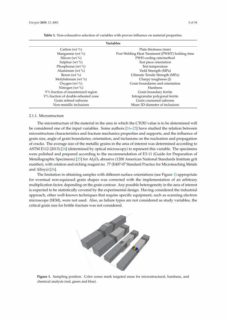
The limitation in obtaining samples with different surface orientations (see Figure 1) appropriatefor eventual non-equiaxed grain shapes was corrected with the implementation of an arbitrarymultiplication factor, depending on the grain contour. Any possible heterogeneity in the area of interestis expected to be statistically covered by the experimental design. Having considered the industrialapproach, other well-known techniques that require specific equipment, such as scanning electronmicroscope (SEM), were not used. Also, as failure types are not considered as study variables, thecritical grain size for brittle fracture was not considered.

Energies 2019, 12, x FOR PEER REVIEW 3 of 18

Manganese (wt %) Post Welding Heat Treatment (PWHT) holding time

Silicon (wt %) PWH cooling rate/method

Sulphur (wt %) Test piece orientation

Phosphorus (wt %) Test temperature

Aluminum (wt %) Yield Strength (MPa)

Boron (wt %) Ultimate Tensile Strength (MPa)

Molybdenum (wt %) Charpy toughness (J)

Oxygen (wt %) Grain boundaries and orientation

Nitrogen (wt %) Hardness

V% fraction of reaustenized region Grain boundary ferrite

V% fraction of double-reheated zone Intragranular polygonal ferrite

Grain refined subzone Grain coarsened subzone

Non-metallic inclusions Mean 3D diameter of inclusions

2.1.1. Microstructure

The microstructure of the material in the area in which the CTOD value is to be determined will

be considered one of the input variables. Some authors [16–23] have studied the relation between

microstructure characteristics and fracture mechanics properties and supports, and the influence of

grain size, angle of grain boundaries, orientation, and inclusions on the nucleation and propagation

of cracks. The average size of the metallic grains in the area of interest was determined according to

ASTM E112 (2013) [24] (determined by optical microscopy) to represent this variable. The specimens

were polished and prepared according to the recommendation of E3-11 (Guide for Preparation of

Metallographic Specimens) [25] for Al2O3 abrasive (1200 American National Standards Institute grit

number), with rotation and etching reagent no. 77 (E407-07 Standard Practice for Microteaching

Metals and Alloys) [26].

The limitation in obtaining samples with different surface orientations (see Figure 1) appropriate

for eventual non-equiaxed grain shapes was corrected with the implementation of an arbitrary

multiplication factor, depending on the grain contour. Any possible heterogeneity in the area of

interest is expected to be statistically covered by the experimental design. Having considered the

industrial approach, other well-known techniques that require specific equipment, such as scanning

electron microscope (SEM), were not used. Also, as failure types are not considered as study

variables, the critical grain size for brittle fracture was not considered.

Figure 1. Sampling position. Color zones mark targeted areas for microstructural, hardness, and

chemical analysis (red, green and blue). Figure 1. Sampling position. Color zones mark targeted areas for microstructural, hardness, andchemical analysis (red, green and blue).

Energies 2019, 12, 4001 4 of 18

2.1.2. Chemical Composition

The chemical composition of the material is a well-known factor that exerts influence on themechanical properties [27–29].

Samples were analyzed by optical emission spectrometry and X-ray diffraction using a Niton ® XL2analyzer and a Spectromax metal analyzer. Results were statistically processed to offer the best-weightedaverage estimator considering the different uncertainties of the testing method and for the followingelements: C, Mn, Si, Cr, Ni, Mo, and V. Both the test procedure and the uncertainty calculation usedwere approved by the testing laboratory. For the implementation of the chemical composition into themathematical model, we considered the influence of the different elements using the carbon equivalent(CE) index, expressed in Equation (1). Among the numerous CE formulae available in the bibliography,we chose American Welding Society (AWS) D1.1 [30], which was cited in [29] and is also known as theInternational Institute of Welding (IIW) carbon equivalent.

This expression was selected considering its precision for mechanical and microstructuralproperties [27]:

CEindex = C +(Mn + Si)

6+

(Cr + Mo + V)

5+

(Ni + Cu)15

(1)

where all values involved represent the mass percentage composition [w/w%]. Therefore, the result isa non-dimensional continuous variable.

2.1.3. Mechanical Strength

The mechanical resistance plays a fundamental role, and forms a constitutive part, in fracturemechanics [31]. Also, the determination and control of its value is a fundamental part of the qualitycontrol of the material properties (for structural materials). Tensile test results were discarded due tothe impossibility to take measurements exclusively in the small area of interest, as all the subsizedspecimens proposed by the standards exceed the capability of the testing machine (too small) ordestroy valuable testing material (too big). Nevertheless, according to numerous publications (e.g.,ASM Handbook for carbon steel), there is a consistent and almost linear relation between ultimatetensile strength (UTS) and hardness. Therefore, hardness measurements according to ASTM E92(Hardness Vickers 10) (2017) [32] were taken from the samples to estimate the mechanical resistance ofthe material. Standardized Vickers indenters (Class B) were used with a load of 98.7 N (HV 10) and anoptical indentation measurement. The average value of a set of three indentations (considering 2 mmof space between tests) were examined for each sample.

2.1.4. Toughness

Previous studies [15,16,33,34] support the relation between impact testing results (measured asCharpy V-notch (CVN) energy values) and fracture toughness. Some correlations have been adoptedby the standards ASME Boiler and Pressure Vessel Code (BPVC) XI (2017) [35] and API 579 [3].

CVN tests, according to ASTM E23 (2018) [36], were performed on the samples. Subsize Charpysimple-beam V-notch impact test specimens were used (2.5 mm, according to Figure A3.1 from ASTME-23), with the notch aligned with the future CTOD sample notch [10]. All tests were performed atroom temperature (between 20 and 25 ◦C) with a 300 J pendulum device. Three specimens (insteadof two) were used for each toughness characterization to ensure representative values (see Figure 1),due to the sample size limitation. Measurement of lateral expansion or the fracture region size wasnot considered.

2.2. Experimental Design

For a multivariate statistical study (with a suitable uncertainty), it is required to reach a determinedcritical mass of input data. This number is undetermined, and it will be verified after the modeling [17].In addition, a wide range that covers the industrial interest is required for the explanatory variables.

Energies 2019, 12, 4001 5 of 18

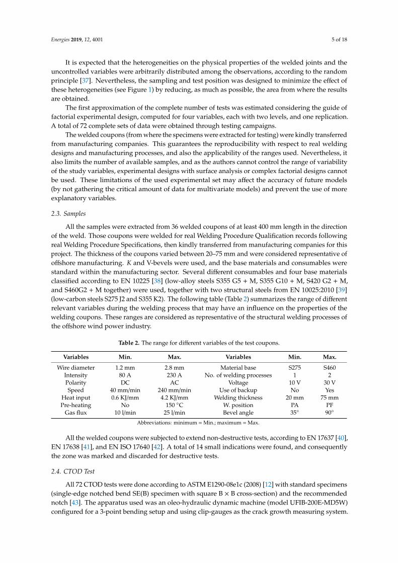
It is expected that the heterogeneities on the physical properties of the welded joints and theuncontrolled variables were arbitrarily distributed among the observations, according to the randomprinciple [37]. Nevertheless, the sampling and test position was designed to minimize the effect ofthese heterogeneities (see Figure 1) by reducing, as much as possible, the area from where the resultsare obtained.

The first approximation of the complete number of tests was estimated considering the guide offactorial experimental design, computed for four variables, each with two levels, and one replication.A total of 72 complete sets of data were obtained through testing campaigns.

The welded coupons (from where the specimens were extracted for testing) were kindly transferredfrom manufacturing companies. This guarantees the reproducibility with respect to real weldingdesigns and manufacturing processes, and also the applicability of the ranges used. Nevertheless, italso limits the number of available samples, and as the authors cannot control the range of variabilityof the study variables, experimental designs with surface analysis or complex factorial designs cannotbe used. These limitations of the used experimental set may affect the accuracy of future models(by not gathering the critical amount of data for multivariate models) and prevent the use of moreexplanatory variables.

2.3. Samples

All the samples were extracted from 36 welded coupons of at least 400 mm length in the directionof the weld. Those coupons were welded for real Welding Procedure Qualification records followingreal Welding Procedure Specifications, then kindly transferred from manufacturing companies for thisproject. The thickness of the coupons varied between 20–75 mm and were considered representative ofoffshore manufacturing. K and V-bevels were used, and the base materials and consumables werestandard within the manufacturing sector. Several different consumables and four base materialsclassified according to EN 10225 [38] (low-alloy steels S355 G5 + M, S355 G10 + M, S420 G2 + M,and S460G2 + M together) were used, together with two structural steels from EN 10025:2010 [39](low-carbon steels S275 J2 and S355 K2). The following table (Table 2) summarizes the range of differentrelevant variables during the welding process that may have an influence on the properties of thewelding coupons. These ranges are considered as representative of the structural welding processes ofthe offshore wind power industry.

Table 2. The range for different variables of the test coupons.

Variables Min. Max. Variables Min. Max.

Wire diameter 1.2 mm 2.8 mm Material base S275 S460Intensity 80 A 230 A No. of welding processes 1 2Polarity DC AC Voltage 10 V 30 VSpeed 40 mm/min 240 mm/min Use of backup No Yes

Heat input 0.6 KJ/mm 4.2 KJ/mm Welding thickness 20 mm 75 mmPre-heating No 150 ◦C W. position PA PF

Gas flux 10 l/min 25 l/min Bevel angle 35◦ 90◦

Abbreviations: minimum = Min.; maximum = Max.

All the welded coupons were subjected to extend non-destructive tests, according to EN 17637 [40],EN 17638 [41], and EN ISO 17640 [42]. A total of 14 small indications were found, and consequentlythe zone was marked and discarded for destructive tests.

2.4. CTOD Test

All 72 CTOD tests were done according to ASTM E1290-08e1c (2008) [12] with standard specimens(single-edge notched bend SE(B) specimen with square B × B cross-section) and the recommendednotch [43]. The apparatus used was an oleo-hydraulic dynamic machine (model UFIB-200E-MD5W)configured for a 3-point bending setup and using clip-gauges as the crack growth measuring system.

Energies 2019, 12, 4001 6 of 18

The testing temperature was in the range of 20–25 ◦C. As Figure 1 shows, the notch was aligned 1 mmfrom the fusion line.

The chosen testing method, ASTM E1290-08e1, calculate the CTOD value with the followingexpression:

δ =1

mσY

K2(1− ν2

)E

+ηCMODApl

CMOD

B(W − a0){1 + Z/(0.8a0 + 0.2W)}

(2)

where Z is the distance of the front face of the SE(B) specimens to the knife-edge measurement point,Apl

CMOD is the plastic area under load from the plastic CMOD curve, and the expression of m is:

m = A0 −A1

(σYSσts

)+ A2

(σYSσts

)2−A3

(σYSσts

)3(3)

where

A0 = 3.18− 0.22( a0

W

), A1 = 4.32− 2.23

( a0

W

), A2 = 4.44− 2.29

( a0

W

), A4 = 2.05− 1.06

( a0

W

)(4)

and

ηCMOD = 3.667− 2.199( a0

W

)+ 0.437

( a0

W

)2, (5)

Alternatives calculations, formulas, and predictions were studied by [33,44–48].All the tests were performed in the private laboratory testing facilities of the TAM group

(accreditation no. 808/LE1532).

2.5. Results

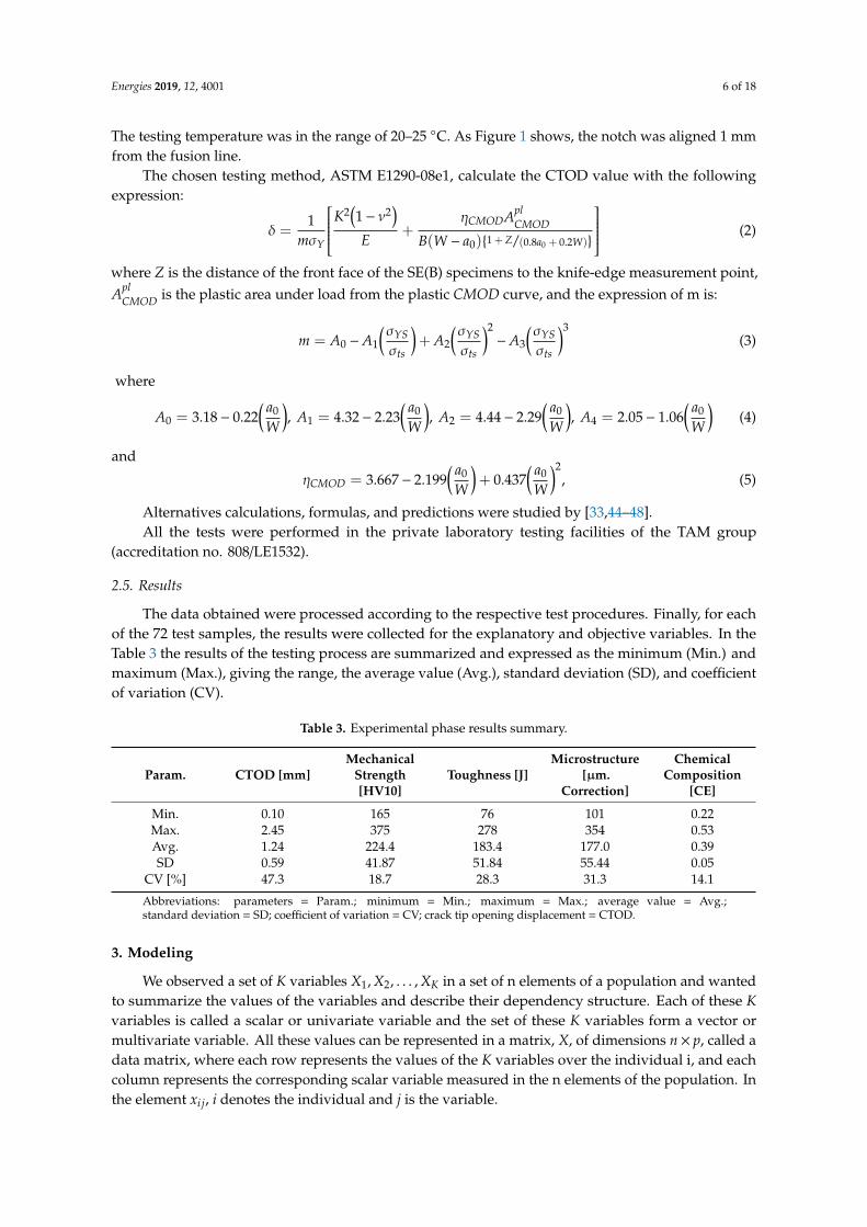
The data obtained were processed according to the respective test procedures. Finally, for eachof the 72 test samples, the results were collected for the explanatory and objective variables. In theTable 3 the results of the testing process are summarized and expressed as the minimum (Min.) andmaximum (Max.), giving the range, the average value (Avg.), standard deviation (SD), and coefficientof variation (CV).

Table 3. Experimental phase results summary.

Param. CTOD [mm]Mechanical

Strength[HV10]

Toughness [J]Microstructure

[µm.Correction]

ChemicalComposition

[CE]

Min. 0.10 165 76 101 0.22Max. 2.45 375 278 354 0.53Avg. 1.24 224.4 183.4 177.0 0.39SD 0.59 41.87 51.84 55.44 0.05

CV [%] 47.3 18.7 28.3 31.3 14.1

Abbreviations: parameters = Param.; minimum = Min.; maximum = Max.; average value = Avg.;standard deviation = SD; coefficient of variation = CV; crack tip opening displacement = CTOD.

3. Modeling

We observed a set of K variables X1, X2, . . . , XK in a set of n elements of a population and wantedto summarize the values of the variables and describe their dependency structure. Each of these Kvariables is called a scalar or univariate variable and the set of these K variables form a vector ormultivariate variable. All these values can be represented in a matrix, X, of dimensions n× p, called adata matrix, where each row represents the values of the K variables over the individual i, and eachcolumn represents the corresponding scalar variable measured in the n elements of the population. Inthe element xi j, i denotes the individual and j is the variable.

Energies 2019, 12, 4001 7 of 18

Next, we proceed to the multivariate analysis of the observations. To do this, we calculate thevector of means X =

[X1 X2 · · · XK

]of dimension p, whose components are the means of each

of the p variables and the covariance matrix. From the matrix of centered data X,

X = X −

11...1

X, (6)

the symmetric and positive semidefinite matrix of covariance S = 1n XTX is calculated.

The objective of describing multivariate data is to understand the dependence between theobjective variable and the explanatory variables. For this we studied:

1. The relationship between pairs of variables;2. Dependence between the objective variable and all the explanatory variables;3. Dependence between the objective variable and the explanatory ones, but eliminating the effect

of some of them.

The pairwise dependence between the variables is measured by the symmetric and positivesemidefinite correlation matrix R

R =

1

r21

r12

1. . . r1K. . . r2K

...... . . .

...rK1 rK2 . . . 1

, r jk =S jk

S jSk(7)

so that there is an exact linear relationship between the variables X j and Xk if∣∣∣r jk

∣∣∣ = 1.It may happen that there are variables that are very dependent on others, in which case it is

convenient to measure their degree of dependence. Assuming that Y = X j is the variable of interest,and calling Y the variable used to estimate Y, the best linear predictor from the other variables, calledthe explanatory variables, is:

Y = β0 + β1X1 + · · ·+ βKXK, (8)

where the parameter βi is determined through the data that we have at our disposal. The problem isfinding the set of parameters that minimizes

∑ni=1 (Yi − Yi)

2, leading to

y = Y −Yx j = X j −X j, j = 1, . . . , K

(9)

and defining y = Y −Y, we have Y − Y = y− y, and Equation (8) can be written as follows

y = α0 + α1x1 + · · ·+ αKxK, (10)

Since minimizing∑n

i=1 (Yi − Yi)2

is equivalent to minimizing∑n

i=1 (yi − yi)2 =

∑ni=1 e2

i , by derivingthis sum with respect to the αk parameters, we obtain a system of p− 1 equations that can be writtenas follows:

n∑i=1

eixil l = 1, . . . , K, l , j (11)

Equation (9) indicates that the prediction errors must not be correlated with the explanatoryvariables, so that the covariance of both is zero, or else the residual vector must be orthogonal to thespace generated by the explanatory variables. By defining the matrix XR, of size n× (p− 1), obtained

Energies 2019, 12, 4001 8 of 18

by eliminating the column in the matrix X corresponding to the variable that we want to predict,y = x j, the parameters are calculated by the normal equation system as follows

α =(XT

RXR)−1

XTRy (12)

and Equation (10), with these coefficients, is the multiple regression equation between variable y = x jand the remaining variables xi, i , j, i = 1, . . . , K.

To express this result based on the X1, . . . , XK variables of Equation (8), we must consider

βi = αi, i = 1, . . . , K

β0 = α0 + Y −K∑

i=1αiXi

(13)

The square of the multiple correlation coefficient (which can be greater than, less than, or equalto the sum of the squares of the simple correlations between variable y and each of the explanatoryvariables) [49] between the variable y = x j and the rest is

R2j = 1−

SSresidSStotal

= 1−1

s j js j j , (14)

where s j j = s2j is the j-th diagonal element of the covariance matrix S and s j j = 1

s2r ( j)

is the j-th diagonal

element of the S−1 matrix, which represents the residual variance of a regression between the j-thvariable and the rest. As each time a variable is added to the model the number of degrees of freedomis reduced and the adjustment is increased, it is necessary to make a correction of this coefficient andcalculate the adjusted R2

j ,

R2j = 1−

SSresid(n−k)SStotal(n−1)

, (15)

where n is the total number of observations and k is the number of model variables; that is, the samecalculation is made, but weighted by the degrees of freedom of the residuals, n − k, and the model,n− 1.

The R-squared RSQ =∑(yi−yi)

2∑(yi−y)2 is a descriptive measure of the predictive capacity of the model,

and for a single explanatory variable is the square of the simple correlation coefficient between thetwo variables.

3.1. Previous Data Processing

Correlation coefficients were determined among the study variables. A high degree of correlationbetween toughness (CVN) and microstructure was observed, which was strongly supported in thebibliography. This relationship also depends on other variables that have not been considered inthis experiment, such as temperature, tension state, or specimen geometry. Therefore, this particularrelation between both variables is exclusive to this experiment and cannot be generalized.

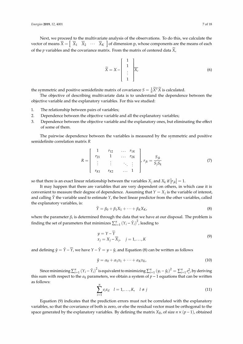
Figure 2 shows the correlation and scatterplot diagrams between all the variables (objectiveand explanatory) taken two-by-two. The kernel density estimation (KDE) representation is also away to estimate the probability density function of a random variable. A strong correlation can beobserved among the CTOD and the explanatory variables, particularly toughness, microstructure, andchemical composition. Excluding the chemical composition, other variables do not seem to follow anormal distribution.

Energies 2019, 12, 4001 9 of 18Energies 2019, 12, x FOR PEER REVIEW 9 of 18

Figure 2. Correlation, kernel density estimation (KDE), and scatterplots (the trendline that best fit

linear relation is represented in blue) among the different variables.

Figure 2 shows the correlation and scatterplot diagrams between all the variables (objective and

explanatory) taken two-by-two. The kernel density estimation (KDE) representation is also a way to

estimate the probability density function of a random variable. A strong correlation can be observed

among the CTOD and the explanatory variables, particularly toughness, microstructure, and

chemical composition. Excluding the chemical composition, other variables do not seem to follow a

normal distribution.

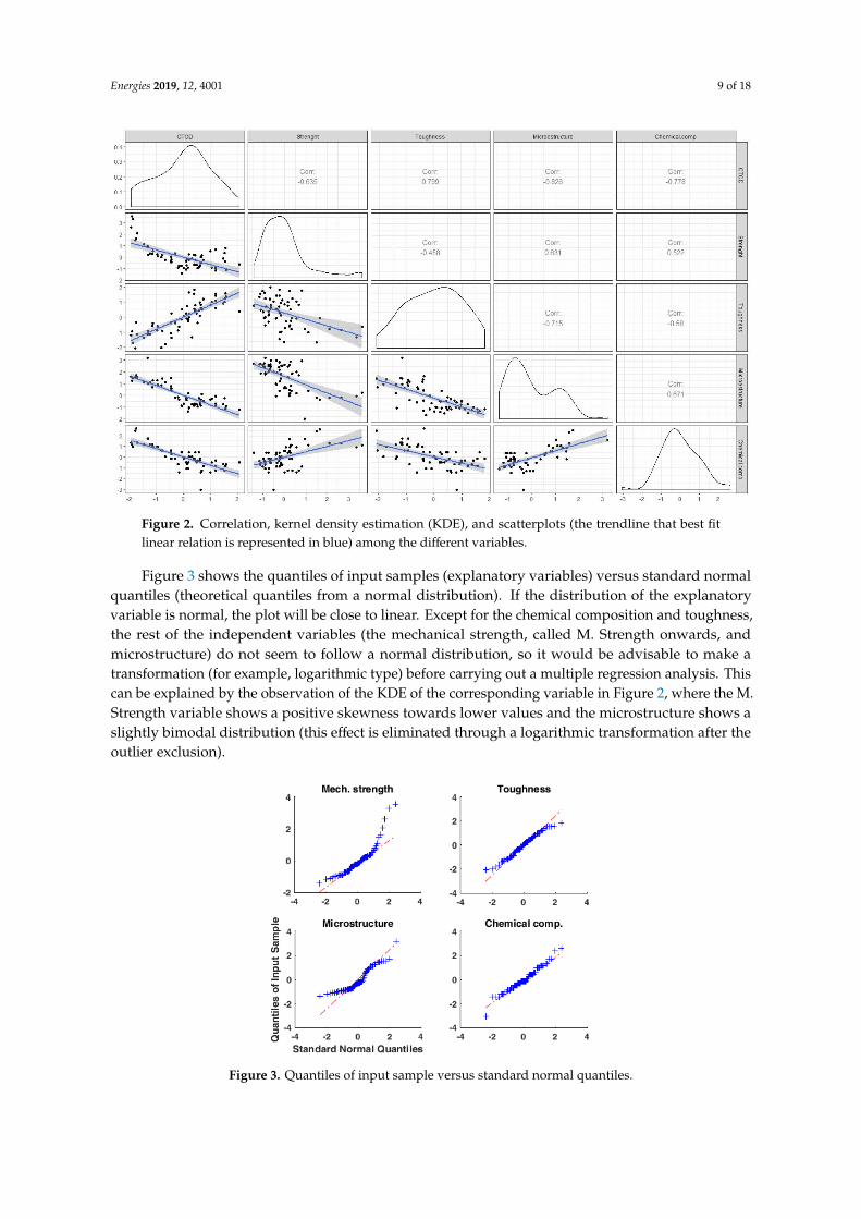
Figure 3 shows the quantiles of input samples (explanatory variables) versus standard normal

quantiles (theoretical quantiles from a normal distribution). If the distribution of the explanatory

variable is normal, the plot will be close to linear. Except for the chemical composition and toughness,

the rest of the independent variables (the mechanical strength, called M. Strength onwards, and

microstructure) do not seem to follow a normal distribution, so it would be advisable to make a

transformation (for example, logarithmic type) before carrying out a multiple regression analysis.

This can be explained by the observation of the KDE of the corresponding variable in Figure 2, where

the M. Strength variable shows a positive skewness towards lower values and the microstructure

shows a slightly bimodal distribution (this effect is eliminated through a logarithmic transformation

after the outlier exclusion).

With the aim of discarding the outliers that could influence observations, the Mahalanobis

distance was used [49,50] for their detection and ten complete data sets were excluded (14%).

Figure 2. Correlation, kernel density estimation (KDE), and scatterplots (the trendline that best fitlinear relation is represented in blue) among the different variables.

Figure 3 shows the quantiles of input samples (explanatory variables) versus standard normalquantiles (theoretical quantiles from a normal distribution). If the distribution of the explanatoryvariable is normal, the plot will be close to linear. Except for the chemical composition and toughness,the rest of the independent variables (the mechanical strength, called M. Strength onwards, andmicrostructure) do not seem to follow a normal distribution, so it would be advisable to make atransformation (for example, logarithmic type) before carrying out a multiple regression analysis. Thiscan be explained by the observation of the KDE of the corresponding variable in Figure 2, where the M.Strength variable shows a positive skewness towards lower values and the microstructure shows aslightly bimodal distribution (this effect is eliminated through a logarithmic transformation after theoutlier exclusion).Energies 2019, 12, x FOR PEER REVIEW 10 of 18

Figure 3. Quantiles of input sample versus standard normal quantiles.

3.2. Linear Regression Models

3.2.1. Linear Model 1

Here, Y is considered as the study variable that may be linearly related with K explanatory

variables 𝑋1, 𝑋2, ⋯ , 𝑋𝐾 through 𝛽0, 𝛽1, 𝛽2, ⋯ , 𝛽𝐾 (regression coefficients). A multiple linear

regression model can be written as:

𝑌 = 𝛽0 + 𝛽1𝑋1 + 𝛽2𝑋2 + ⋯ + 𝛽𝐾𝑋𝐾 + 𝑒 (16)

where e is the difference between the fitted relationship and the observations [51].

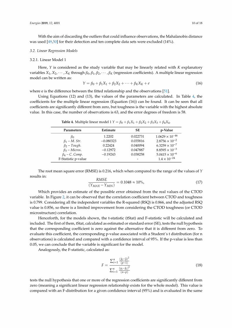
Using Equations (12) and (13), the values of the parameters are calculated. In Table 4, the

coefficients for the multiple linear regression (Equation (16)) can be found. It can be seen that all

coefficients are significantly different from zero, but toughness is the variable with the highest

absolute value. In this case, the number of observations is 63, and the error degrees of freedom is 58.

The root mean square error (RMSE) is 0.216, which when compared to the range of the values of

Y results in:

𝑅𝑀𝑆𝐸

(𝑌𝑀𝐴𝑋 − 𝑌𝑀𝐼𝑁)= 0.1048 ≈ 10%, (17)

Which provides an estimate of the possible error obtained from the real values of the CTOD

variable. In Figure 2, it can be observed that the correlation coefficient between CTOD and toughness

is 0.799. Considering all the independent variables the R-squared (RSQ) is 0.866, and the adjusted

RSQ value is 0.856, so there is a limited improvement from considering the CTOD toughness (or

CTOD microstructure) correlation.

Table 4. Multiple linear model 1 𝑌 = 𝛽0 + 𝛽1𝑋1 + 𝛽2𝑋2 + 𝛽3𝑋3 + 𝛽4𝑋4.

Parameters Estimate SE p-Value

𝛽0 1.2202 0.022731 1.0629 × 10-46

𝛽1 − 𝑀. 𝑆𝑡𝑟. −0.080323 0.035816 2.8756 × 10-2

𝛽2 − 𝑇𝑜𝑢𝑔ℎ. 0.22424 0.040094 6.3259 × 10-7

𝛽3 − 𝑀𝑖𝑐𝑟𝑜𝑠. −0.12972 0.047887 8.8595 × 10-3

𝛽4 − 𝐶. 𝐶𝑜𝑚𝑝. −0.19243 0.038258 5.0415 × 10-6

F-Statistic p-value - - 1.4 × 10-24

Figure 3. Quantiles of input sample versus standard normal quantiles.

Energies 2019, 12, 4001 10 of 18

With the aim of discarding the outliers that could influence observations, the Mahalanobis distancewas used [49,50] for their detection and ten complete data sets were excluded (14%).

3.2. Linear Regression Models

3.2.1. Linear Model 1

Here, Y is considered as the study variable that may be linearly related with K explanatoryvariables X1, X2, · · · , XK through β0, β1, β2, · · · , βK (regression coefficients). A multiple linear regressionmodel can be written as:

Y = β0 + β1X1 + β2X2 + · · ·+ βKXK + e (16)

where e is the difference between the fitted relationship and the observations [51].Using Equations (12) and (13), the values of the parameters are calculated. In Table 4, the

coefficients for the multiple linear regression (Equation (16)) can be found. It can be seen that allcoefficients are significantly different from zero, but toughness is the variable with the highest absolutevalue. In this case, the number of observations is 63, and the error degrees of freedom is 58.

Table 4. Multiple linear model 1 Y = β0 + β1X1 + β2X2 + β3X3 + β4X4.

Parameters Estimate SE p-Value

β0 1.2202 0.022731 1.0629 × 10−46

β1 −M. Str. −0.080323 0.035816 2.8756 × 10−2

β2 − Tough. 0.22424 0.040094 6.3259 × 10−7

β3 −Micros. −0.12972 0.047887 8.8595 × 10−3

β4 −C. Comp. −0.19243 0.038258 5.0415 × 10−6

F-Statistic p-value - - 1.4 × 10−24

The root mean square error (RMSE) is 0.216, which when compared to the range of the values of Yresults in:

RMSE(YMAX −YMIN)

= 0.1048 ≈ 10%, (17)

Which provides an estimate of the possible error obtained from the real values of the CTODvariable. In Figure 2, it can be observed that the correlation coefficient between CTOD and toughnessis 0.799. Considering all the independent variables the R-squared (RSQ) is 0.866, and the adjusted RSQvalue is 0.856, so there is a limited improvement from considering the CTOD toughness (or CTODmicrostructure) correlation.

Henceforth, for the models shown, the t-statistic (tStat) and F-statistic will be calculated andincluded. The first of them, tStat, calculated as estimated or standard error (SE), tests the null hypothesisthat the corresponding coefficient is zero against the alternative that it is different from zero. Toevaluate this coefficient, the corresponding p-value associated with a Student´s t distribution (for nobservations) is calculated and compared with a confidence interval of 95%. If the p-value is less than0.05, we can conclude that the variable is significant for the model.

Analogously, the F-statistic, calculated as:

F =

∑ni=1

(yi−y)2

(p−1)∑ni=1

(yi−yi)2

(n−p)

(18)

tests the null hypothesis that one or more of the regression coefficients are significantly different fromzero (meaning a significant linear regression relationship exists for the whole model). This value iscompared with an F-distribution for a given confidence interval (95%) and is evaluated in the same

Energies 2019, 12, 4001 11 of 18

way as the t-statistic (associated p-value less than 0.05). The F-distribution is more appropriate thanChi-square tests for small data sets [52].

Two different methods were used to verify that the obtained model was independent of the chosendata population: cross-validation and training-test samples.

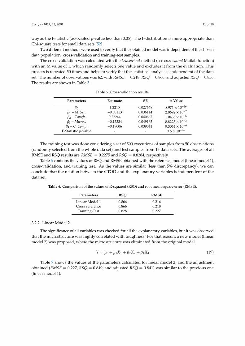
The cross-validation was calculated with the LeaveMout method (see crossvalind Matlab function)with an M value of 1, which randomly selects one value and excludes it from the evaluation. Thisprocess is repeated 50 times and helps to verify that the statistical analysis is independent of the dataset. The number of observations was 62, with RMSE = 0.218, RSQ = 0.866, and adjusted RSQ = 0.856.The results are shown in Table 5.

Table 5. Cross-validation results.

Parameters Estimate SE p-Value

β0 1.2215 0.027668 8.971 × 10−46

β1 −M. Str. −0.08113 0.036144 2.8692 × 10−2

β2 − Tough. 0.22244 0.040667 1.0436 × 10−6

β3 −Micros. −0.13334 0.049165 8.8225 × 10−3

β4 −C. Comp. −0.19006 0.039041 9.3064 × 10−6

F-Statistic p-value - - 3.5 × 10−24

The training test was done considering a set of 500 executions of samples from 50 observations(randomly selected from the whole data set) and test samples from 13 data sets. The averages of allRMSE and RSQ results are

________RMSE = 0.2275 and

_____RSQ = 0.8284, respectively.

Table 6 contains the values of RSQ and RMSE obtained with the reference model (linear model 1),cross-validation, and training test. As the values are similar (less than 5% discrepancy), we canconclude that the relation between the CTOD and the explanatory variables is independent of thedata set.

Table 6. Comparison of the values of R-squared (RSQ) and root mean square error (RMSE).

Parameters RSQ RMSE

Linear Model 1 0.866 0.216Cross reference 0.866 0.218Training-Test 0.828 0.227

3.2.2. Linear Model 2

The significance of all variables was checked for all the explanatory variables, but it was observedthat the microstructure was highly correlated with toughness. For that reason, a new model (linearmodel 2) was proposed, where the microstructure was eliminated from the original model.

Y = β0 + β1X1 + β2X2 + β4X4 (19)

Table 7 shows the values of the parameters calculated for linear model 2, and the adjustmentobtained (RMSE = 0.227, RSQ = 0.849, and adjusted RSQ = 0.841) was similar to the previous one(linear model 1).

Energies 2019, 12, 4001 12 of 18

Table 7. Multiple linear regression model 2 Y = β0 + β1X1 + β2X2 + β4X4.

Parameters Estimate SE p-Value

β0 1.2202 0.028657 5.353 × 10−46

β1 −M. Str. −0.11829 0.034686 1.1768 × 10−3

β2 − Tough. 0.27944 0.036337 1.8301 × 10−10

β4 −C. Comp. −0.22775 0.03785 1.2105 × 10−7

F-Statistic p-value - - 3.79 × 10−24

3.2.3. Linear Models 3 and 4

As the value of parameter β1 (coefficient of the mechanical strength) in linear model 1 wassmall compared to the values of the rest of the parameters, it was that the corresponding variable beeliminated to obtain a new model (linear model 3), considering that its contribution to the value of theCTOD variable was small. The values of the coefficients of linear model 3 are represented in Table 8.

Table 8. Linear regression model 3 Y = β0 + β2X2 + β3X3 + β4X4.

Parameters Estimate SE p-Value

β0 1.2202 0.028146 1.9133 × 10−46

β2 − Tough. 0.22225 0.04143 1.4246 × 10−6

β3 −Micros. −0.17174 0.045549 3.793 × 10−4

β4 −C. Comp. −0.20715 0.038957 1.961 × 10−6

F-Statistic p-value - - 1.32 × 10−24

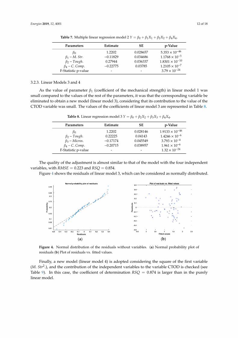
The quality of the adjustment is almost similar to that of the model with the four independentvariables, with RMSE = 0.223 and RSQ = 0.854.

Figure 4 shows the residuals of linear model 3, which can be considered as normally distributed.

Energies 2019, 12, x FOR PEER REVIEW 12 of 18

𝑌 = 𝛽0 + 𝛽1𝑋1 + 𝛽2𝑋2 + 𝛽4𝑋4 (19)

Table 7 shows the values of the parameters calculated for linear model 2, and the adjustment

obtained (𝑅𝑀𝑆𝐸 = 0.227, 𝑅𝑆𝑄 = 0.849, and adjusted 𝑅𝑆𝑄 = 0.841) was similar to the previous one

(linear model 1).

Table 7. Multiple linear regression model 2 𝑌 = 𝛽0 + 𝛽1𝑋1 + 𝛽2𝑋2 + 𝛽4𝑋4.

Parameters Estimate SE p-Value

𝛽0 1.2202 0.028657 5.353 × 10−46

𝛽1 − 𝑀. 𝑆𝑡𝑟. −0.11829 0.034686 1.1768 × 10−3

𝛽2 − 𝑇𝑜𝑢𝑔ℎ. 0.27944 0.036337 1.8301 × 10−10

𝛽4 − 𝐶. 𝐶𝑜𝑚𝑝. −0.22775 0.03785 1.2105 × 10−7

F-Statistic p-value - - 3.79 × 10−24

3.2.3. Linear Models 3 and 4

As the value of parameter 𝛽1 (coefficient of the mechanical strength) in linear model 1 was small

compared to the values of the rest of the parameters, it was that the corresponding variable be

eliminated to obtain a new model (linear model 3), considering that its contribution to the value of

the CTOD variable was small. The values of the coefficients of linear model 3 are represented in Table

8.

Table 8. Linear regression model 3 𝑌 = 𝛽0 + 𝛽2𝑋2 + 𝛽3𝑋3 + 𝛽4𝑋4.

Parameters Estimate SE p-Value

𝛽0 1.2202 0.028146 1.9133 × 10−46

𝛽2 − 𝑇𝑜𝑢𝑔ℎ. 0.22225 0.04143 1.4246 × 10−6

𝛽3 − 𝑀𝑖𝑐𝑟𝑜𝑠. −0.17174 0.045549 3.793 × 10−4

𝛽4 − 𝐶. 𝐶𝑜𝑚𝑝. −0.20715 0.038957 1.961 × 10−6

F-Statistic p-value - - 1.32 × 10−24

The quality of the adjustment is almost similar to that of the model with the four independent

variables, with 𝑅𝑀𝑆𝐸 = 0.223 and 𝑅𝑆𝑄 = 0.854.

Figure 4 shows the residuals of linear model 3, which can be considered as normally distributed.

(a)

(b)

Figure 4. Normal distribution of the residuals without variables. (a) Normal probability plot of

residuals (b) Plot of residuals vs. fitted values.

Figure 4. Normal distribution of the residuals without variables. (a) Normal probability plot ofresiduals (b) Plot of residuals vs. fitted values.

Finally, a new model (linear model 4) is adopted considering the square of the first variable(M. Str2.), and the contribution of the independent variables to the variable CTOD is checked (seeTable 9). In this case, the coefficient of determination RSQ = 0.874 is larger than in the purelylinear model.

Energies 2019, 12, 4001 13 of 18

Table 9. Linear regression model 4 Y = β0 + β1X21 + β2X2 + β3X3 + β4X4.

Parameters Estimate SE p-Value

β0 1.2584 0.029113 8.0522 × 10−46

β1 −M. Str2. −0.038872 0.012639 3.2021 × 10−3

β2 − Tough. 0.21641 0.038792 6.6704 × 10−7

β3 −Micros. −0.1562 0.042897 5.7976 × 10−4

β4 −C. Comp. −0.19142 0.036789 2.68 × 10−6

F-Statistic p-value - - 1.97 × 10−25

Other tests have been done with different interactions between variables, but they do not improvethe results.

3.3. Multivariate Adaptative Regression Splines (MARS)

Multivariate adaptive regression splines (MARS) is a non-parametric modeling method thatextends the linear model (incorporating nonlinearities and interactions). It is a generalization of therecursive partitioning regression (RPR), which splits up the space of the explanatory variables intodifferent subregions. MARS generates cut points for the variables. These knots are identified throughbaseline functions, which indicates the beginning and end of a region.

In each region in which the space is divided, a base linear function of one variable is adjusted.The final model is constituted from a combination of the generated base functions [53].

The general expression of the model is:

Y =k∑

i=1

ciBi(x) , (20)

where ci is the constant coefficient and Bi is the base function.A MARS model was applied using cubic splines. This method considers nonlinear relationships

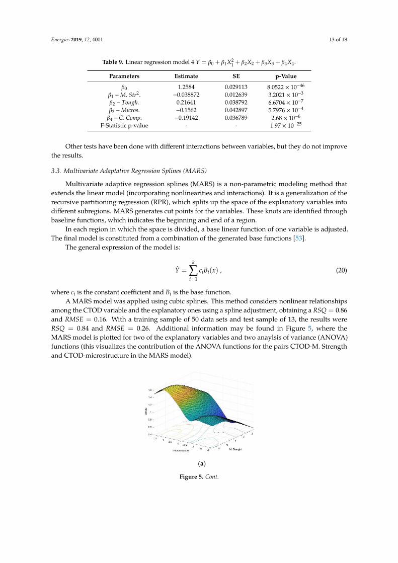
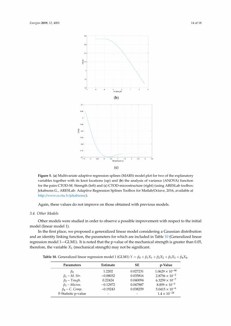
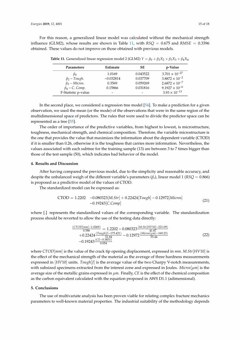
among the CTOD variable and the explanatory ones using a spline adjustment, obtaining a RSQ = 0.86and RMSE = 0.16. With a training sample of 50 data sets and test sample of 13, the results wereRSQ = 0.84 and RMSE = 0.26. Additional information may be found in Figure 5, where theMARS model is plotted for two of the explanatory variables and two anaylsis of variance (ANOVA)functions (this visualizes the contribution of the ANOVA functions for the pairs CTOD-M. Strengthand CTOD-microstructure in the MARS model).

Energies 2019, 12, x FOR PEER REVIEW 13 of 18

Finally, a new model (linear model 4) is adopted considering the square of the first variable

(𝑀. 𝑆𝑡𝑟2.), and the contribution of the independent variables to the variable CTOD is checked (see

Table 9). In this case, the coefficient of determination 𝑅𝑆𝑄 = 0.874 is larger than in the purely linear

model.

Table 9. Linear regression model 4 𝑌 = 𝛽0 + 𝛽1𝑋12 + 𝛽2𝑋2 + 𝛽3𝑋3 + 𝛽4𝑋4.

Parameters Estimate SE p-Value

𝛽0 1.2584 0.029113 8.0522 × 10−46

𝛽1 − 𝑀. 𝑆𝑡𝑟2. −0.038872 0.012639 3.2021 × 10−3

𝛽2 − 𝑇𝑜𝑢𝑔ℎ. 0.21641 0.038792 6.6704 × 10−7

𝛽3 − 𝑀𝑖𝑐𝑟𝑜𝑠. −0.1562 0.042897 5.7976 × 10−4

𝛽4 − 𝐶. 𝐶𝑜𝑚𝑝. −0.19142 0.036789 2.68 × 10−6

F-Statistic p-value - - 1.97 × 10−25

Other tests have been done with different interactions between variables, but they do not

improve the results.

3.3. Multivariate Adaptative Regression Splines (MARS)

Multivariate adaptive regression splines (MARS) is a non-parametric modeling method that

extends the linear model (incorporating nonlinearities and interactions). It is a generalization of the

recursive partitioning regression (RPR), which splits up the space of the explanatory variables into

different subregions. MARS generates cut points for the variables. These knots are identified through

baseline functions, which indicates the beginning and end of a region.

In each region in which the space is divided, a base linear function of one variable is adjusted.

The final model is constituted from a combination of the generated base functions [53].

The general expression of the model is:

�� = ∑ 𝑐𝑖𝐵𝑖(𝑥) ,

𝑘

𝑖=1

(20)

where ci is the constant coefficient and Bi is the base function.

A MARS model was applied using cubic splines. This method considers nonlinear relationships

among the CTOD variable and the explanatory ones using a spline adjustment, obtaining a 𝑅𝑆𝑄 =

0.86 and 𝑅𝑀𝑆𝐸 = 0.16. With a training sample of 50 data sets and test sample of 13, the results were

𝑅𝑆𝑄 = 0.84 and 𝑅𝑀𝑆𝐸 = 0.26. Additional information may be found in Figure 5, where the MARS

model is plotted for two of the explanatory variables and two anaylsis of variance (ANOVA)

functions (this visualizes the contribution of the ANOVA functions for the pairs CTOD-M. Strength

and CTOD-microstructure in the MARS model).

(a)

Figure 5. Cont.

Energies 2019, 12, 4001 14 of 18Energies 2019, 12, x FOR PEER REVIEW 14 of 18

(b)

(c)

Figure 5. (a) Multivariate adaptive regression splines (MARS) model plot for two of the explanatory

variables together with its knot locations (up) and (b) the analysis of variance (ANOVA) function for

the pairs CTOD-M. Strength (left) and (c) CTOD-microstructure (right) (using ARESLab toolbox:

Jekabsons G., ARESLab: Adaptive Regression Splines Toolbox for Matlab/Octave, 2016, available at

http://www.cs.rtu.lv/jekabsons/).

Again, these values do not improve on those obtained with previous models.

3.4. Other Models

Other models were studied in order to observe a possible improvement with respect to the initial

model (linear model 1).

In the first place, we proposed a generalized linear model considering a Gaussian distribution

and an identity linking function, the parameters for which are included in Table 10 (Generalized

linear regression model 1—GLM1). It is noted that the p-value of the mechanical strength is greater

than 0.05, therefore, the variable 𝑋1 (mechanical strength) may not be significant.

Table 10. Generalized linear regression model 1 (GLM1) 𝑌 = 𝛽0 + 𝛽1𝑋1 + 𝛽2𝑋2 + 𝛽3𝑋3 + 𝛽4𝑋4.

Parameters Estimate SE p-Value

𝛽0 1.2202 0.027231 1.0629 × 10−46

𝛽1 − 𝑀. 𝑆𝑡𝑟. −0.08032 0.035816 2.8756 × 10−2

𝛽2 − 𝑇𝑜𝑢𝑔ℎ. 0.22424 0.040094 6.3259 × 10−7

𝛽3 − 𝑀𝑖𝑐𝑟𝑜𝑠. −0.12972 0.047887 8.859 × 10−3

𝛽4 − 𝐶. 𝐶𝑜𝑚𝑝. −0.19243 0.038259 5.0415 × 10−6

F-Statistic p-value - - 1.4 × 10−24

Figure 5. (a) Multivariate adaptive regression splines (MARS) model plot for two of the explanatoryvariables together with its knot locations (up) and (b) the analysis of variance (ANOVA) functionfor the pairs CTOD-M. Strength (left) and (c) CTOD-microstructure (right) (using ARESLab toolbox:Jekabsons G., ARESLab: Adaptive Regression Splines Toolbox for Matlab/Octave, 2016, available athttp://www.cs.rtu.lv/jekabsons/).

Again, these values do not improve on those obtained with previous models.

3.4. Other Models

Other models were studied in order to observe a possible improvement with respect to the initialmodel (linear model 1).

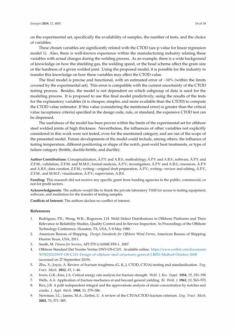
In the first place, we proposed a generalized linear model considering a Gaussian distributionand an identity linking function, the parameters for which are included in Table 10 (Generalized linearregression model 1—GLM1). It is noted that the p-value of the mechanical strength is greater than 0.05,therefore, the variable X1 (mechanical strength) may not be significant.

Table 10. Generalized linear regression model 1 (GLM1) Y = β0 + β1X1 + β2X2 + β3X3 + β4X4.

Parameters Estimate SE p-Value

β0 1.2202 0.027231 1.0629 × 10−46

β1 −M. Str. −0.08032 0.035816 2.8756 × 10−2

β2 − Tough. 0.22424 0.040094 6.3259 × 10−7

β3 −Micros. −0.12972 0.047887 8.859 × 10−3

β4 −C. Comp. −0.19243 0.038259 5.0415 × 10−6

F-Statistic p-value - - 1.4 × 10−24

Energies 2019, 12, 4001 15 of 18

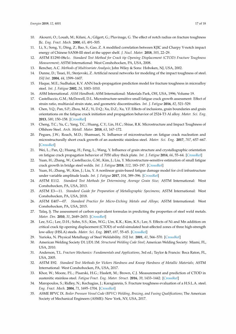
For this reason, a generalized linear model was calculated without the mechanical strengthinfluence (GLM2), whose results are shown in Table 11, with RSQ = 0.675 and RMSE = 0.3396obtained. These values do not improve on those obtained with previous models.

Table 11. Generalized linear regression model 2 (GLM2) Y = β0 + β2X2 + β3X3 + β4X4.

Parameters Estimate SE p-Value

β0 1.0169 0.043522 3.701 × 10−27

β2 − Tough. −0.032814 0.037709 3.8872 × 10−2

β3 −Micros. 0.3569 0.059269 2.6872 × 10−7

β4 −C. Comp. 0.15866 0.031816 9.1927 × 10−6

F-Statistic p-value - - 3.93 × 10−13

In the second place, we considered a regression tree model [54]. To make a prediction for a givenobservation, we used the mean (or the mode) of the observations that were in the same region of themultidimensional space of predictors. The rules that were used to divide the predictor space can berepresented as a tree [55].

The order of importance of the predictive variables, from highest to lowest, is microstructure,toughness, mechanical strength, and chemical composition. Therefore, the variable microstructure isthe one that provides the value that maximizes the information about the dependent variable (CTOD)if it is smaller than 0.26, otherwise it is the toughness that carries more information. Nevertheless, thevalues associated with each subtree for the training sample (13) are between 3 to 7 times bigger thanthose of the test sample (50), which indicates bad behavior of the model.

4. Results and Discussion

After having compared the previous model, due to the simplicity and reasonable accuracy, anddespite the unbalanced weigh of the different variable’s parameters (βi), linear model 1 (RSQ = 0.866)is proposed as a predictive model of the values of CTOD.

The standardized model can be expressed as:

CTOD = 1.2202 −0.080323[M.Str] + 0.22424[Tough] − 0.12972[Micros]−0.19243[C.Comp]

(21)

where [.] represents the standardized values of the corresponding variable. The standardizationprocess should be reverted to allow the use of the testing data directly:

(CTOD[mm]−1.0269)0.586 = 1.2202− 0.080323 (M.Str[HV10]−221.09)

41.87

+0.22424 (Tough[J]−175.421)51.84 − 0.12972 (Micros[µm]−169.23)

55.44

−0.19243 (CE−0.3831)0.054

(22)

where CTOD[mm] is the value of the crack tip opening displacement, expressed in mm. M.Str[HV10] isthe effect of the mechanical strength of the material as the average of three hardness measurementsexpressed in [HV10] units. Tough[J] is the average value of the two Charpy V-notch measurements,with subsized specimens extracted from the interest zone and expressed in Joules. Micros[µm] is theaverage size of the metallic grains expressed in µm. Finally, CE is the effect of the chemical compositionas the carbon equivalent calculated with the equation proposed in AWS D1.1 (adimensional).

5. Conclusions

The use of multivariate analysis has been proven viable for relating complex fracture mechanicsparameters to well-known material properties. The industrial suitability of the methodology depends

Energies 2019, 12, 4001 16 of 18

on the experimental set, specifically the availability of samples, the number of tests, and the choiceof variables.

These chosen variables are significantly related with the CTOD (see p-value for linear regressionmodel 1). Also, there is well-known experience within the manufacturing industry relating thesevariables with actual changes during the welding process. As an example, there is a wide backgroundof knowledge on how the shielding gas, the welding speed, or the bead scheme affect the grain sizeor the hardness of a given welded joint. Using the proposed model, it is possible for the industry totransfer this knowledge on how these variables may affect the CTOD value.

The final model is precise and functional, with an estimated error of ~10% (within the limitscovered by the experimental set). This error is compatible with the current uncertainty of the CTODtesting process. Besides, the model is not dependent on which subgroup of data is used for themodeling process. It is proposed to use this final model predictively, using the results of the testsfor the explanatory variables (it is cheaper, simpler, and more available than the CTOD) to computethe CTOD value estimator. If this value (considering the mentioned error) is greater than the criticalvalue (acceptance criteria) specified in the design code, rule, or standard, the expensive CTOD test canbe dispensed.

The usefulness of the model has been proven within the limits of the experimental set for offshoresteel welded joints of high thickness. Nevertheless, the influences of other variables not explicitlyconsidered in this work were not tested, even for the mentioned category, and are out of the scope ofthe presented model. Future developments of the model could include, among others, the influence oftesting temperature, different positioning or shape of the notch, post-weld heat treatments, or type offailure category (brittle, ductile-brittle, and ductile).

Author Contributions: Conceptualization, Á.P.V. and A.B.S.; methodology, Á.P.V. and A.B.S.; software, Á.P.V. andZ.F.M.; validation, Z.F.M. and M.M.F.; formal analysis, Á.P.V.; investigation, Á.P.V. and A.B.S.; resources, Á.P.V.and A.B.S.; data curation, Z.F.M.; writing—original draft preparation, Á.P.V.; writing—review and editing, Á.P.V.,Z.F.M., and M.M.F.; visualization, Á.P.V.; supervision, A.B.S.

Funding: This research did not receive any specific grant from funding agencies in the public, commercial, ornot-for-profit sectors.

Acknowledgments: The authors would like to thank the private laboratory TAM for access to testing equipment,software, and mediation for the transfer of testing samples.

Conflicts of Interest: The authors declare no conflict of interest.

References

1. Rodrigues, P.E.; Wong, W.K.; Rogerson, J.H. Weld Defect Distributions in Offshore Platforms and TheirRelevance to Reliability Studies, Quality Control and In-Service Inspection. In Proceedings of the OffshoreTechnology Conference, Houston, TX, USA, 5–8 May 1980.

2. American Bureau of Shipping. Design Standards for Offshore Wind Farms; American Bureau of Shipping:Huston Texas, USA, 2011.

3. Smith, M. Fitness for Service, API 579-1/ASME FFS-1. 2007.4. Offshore Standard Det Norske Veritas DNV-OS-C101. Available online: https://www.scribd.com/document/

50782302/DNV-OS-C101-Design-of-offshore-steel-structures-general-LRFD-Method-October-2008(accessed on 27 September 2019).

5. Zhu, X.; Joyce, A. Review of fracture toughness (G, K, J, CTOD, CTOA) testing and standardization. Eng.Fract. Mech. 2012, 85, 1–46.

6. Irwin, G.R.; Kies, J.A. Critical energy rate analysis for fracture strength. Weld. J. Res. Suppl. 1954, 19, 193–198.7. Wells, A.A. Application of fracture mechanics at and beyond general yielding. Br. Weld. J. 1963, 10, 563–570.8. Rice, J.R. A path independent integral and the approximate analysis of strain concentration by notches and

cracks. J. Appl. Mech. 1968, 35, 379–386.9. Newman, J.C.; James, M.A.; Zerbst, U. A review of the CTOA/CTOD fracture criterion. Eng. Fract. Mech.

2003, 70, 371–385.

Energies 2019, 12, 4001 17 of 18

10. Akourri, O.; Louah, M.; Kifani, A.; Gilgert, G.; Pluvinage, G. The effect of notch radius on fracture toughnessJIc. Eng. Fract. Mech. 2000, 65, 491–505.

11. Li, X.; Song, Y.; Ding, Z.; Bao, S.; Gao, Z. A modified correlation between KJIC and Charpy V-notch impactenergy of Chinese SA508-III steel at the upper shelf. J. Nucl. Mater. 2018, 505, 22–29.

12. ASTM E1290-08e1c. Standard Test Method for Crack tip Opening Displacement (CTOD) Fracture ToughnessMeasurement; ASTM International: West Conshohocken, PA, USA, 2008.

13. Rencher, A.C. Methods of Multivariate Analysis; John Wiley & Sons: Hoboken, NJ, USA, 2002.14. Dunne, D.; Tsuei, H.; Sterjovski, Z. Artificial neural networks for modeling of the impact toughness of steel.

ISIJ Int. 2004, 44, 1599–1607.15. Haque, M.E.; Sudhakar, K.V. ANN back-propagation prediction model for fracture toughness in microalloy

steel. Int. J. Fatigue 2002, 24, 1003–1010.16. ASM International. ASM Handbook; ASM International: Materials Park, OH, USA, 1996; Volume 19.17. Castelluccio, G.M.; McDowell, D.L. Microstructure-sensitive small fatigue crack growth assessment: Effect of

strain ratio, multiaxial strain state, and geometric discontinuities. Int. J. Fatigue 2016, 82, 521–529.18. Chen, Y.Q.; Pan, S.P.; Zhou, M.Z.; Yi, D.Q.; Xu, D.Z.; Xu, Y.F. Effects of inclusions, grain boundaries and grain

orientations on the fatigue crack initiation and propagation behavior of 2524-T3 Al alloy. Mater. Sci. Eng.2013, 580, 150–158. [CrossRef]

19. Cheng, T.C.; Yu, C.; Yang, T.C.; Huang, C.Y.; Lin, H.C.; Shiue, R.K. Microstructure and Impact Toughness ofOffshore Steel. Arch. Metall. Mater. 2018, 63, 167–172.

20. Pegues, J.W.; Roach, M.D.; Shamsaei, N. Influence of microstructure on fatigue crack nucleation andmicrostructurally short crack growth of an austenitic stainless steel. Mater. Sci. Eng. 2017, 707, 657–667.[CrossRef]

21. Wei, L.; Pan, Q.; Huang, H.; Feng, L.; Wang, Y. Influence of grain structure and crystallographic orientationon fatigue crack propagation behavior of 7050 alloy thick plate. Int. J. Fatigue 2014, 66, 55–64. [CrossRef]

22. Yuan, H.; Zhang, W.; Castelluccio, G.M.; Kim, J.; Liu, Y. Microstructure-sensitive estimation of small fatiguecrack growth in bridge steel welds. Int. J. Fatigue 2018, 112, 183–197. [CrossRef]

23. Yuan, H.; Zhang, W.; Kim, J.; Liu, Y. A nonlinear grain-based fatigue damage model for civil infrastructureunder variable amplitude loads. Int. J. Fatigue 2017, 104, 389–396. [CrossRef]

24. ASTM E112. Standard Test Methods for Determining Average Grain Size; ASTM International: WestConshohocken, PA, USA, 2013.

25. ASTM E3—11. Standard Guide for Preparation of Metallographic Specimens; ASTM International: WestConshohocken, PA, USA, 2018.

26. ASTM E407—07. Standard Practice for Micro-Etching Metals and Alloys; ASTM International: WestConshohocken, PA, USA, 2015.

27. Talas, S. The assessment of carbon equivalent formulas in predicting the properties of steel weld metals.Mater. Des. 2010, 31, 2649–2653. [CrossRef]

28. Lee, S.G.; Lee, D.H.; Sohn, S.S.; Kim, W.G.; Um, K.K.; Kim, K.S.; Lee, S. Effects of Ni and Mn addition oncritical crack tip opening displacement (CTOD) of weld-simulated heat-affected zones of three high-strengthlow-alloy (HSLA) steels. Mater. Sci. Eng. 2017, 697, 55–65. [CrossRef]

29. Yurioka, N. Physical Metallurgy of Steel Weldability. ISIJ Int. 2001, 41, 566–570. [CrossRef]30. American Welding Society D1.1/D1.1M. Structural Welding Code Steel; American Welding Society: Miami, FL,

USA, 2010.31. Anderson, T.L. Fracture Mechanics: Fundamentals and Applications, 3rd ed.; Taylor & Francis: Boca Raton, FL,

USA, 2005.32. ASTM E92. Standard Test Methods for Vickers Hardness and Knoop Hardness of Metallic Materials; ASTM

International: West Conshohocken, PA, USA, 2017.33. Khor, W.; Moore, P.L.; Pisarski, H.G.; Haslett, M.; Brown, C.J. Measurement and prediction of CTOD in

austenitic stainless steel. Fatigue Fract. Eng. Mater. Struct. 2016, 39, 1433–1442. [CrossRef]34. Maropoulos, S.; Ridley, N.; Kechagias, J.; Karagiannis, S. Fracture toughness evaluation of a H.S.L.A. steel.

Eng. Fract. Mech. 2004, 71, 1695–1704. [CrossRef]35. ASME BPVC IX. Boiler Pressure Vessel Code (BPVC) Welding, Brazing, and Fusing Qualifications; The American

Society of Mechanical Engineers (ASME): New York, NY, USA, 2017.

Energies 2019, 12, 4001 18 of 18

36. ASTM E23. Standard Test Methods for Notched Bar Impact Testing of Metallic Materials; ASTM International:West Conshohocken, PA, USA, 2018.

37. Yang, Y.Y.; Mahfouf, M.; Panoutsos, G. Probabilistic Characterization of Model Error Using Gaussian MixtureModel—with Application to Charpy Impact Energy Prediction for Alloy Steel. Control Eng. Pract. 2012, 20,82–92. [CrossRef]

38. EN 10225. Weldable Structural Steels for Fixed Offshore Structures; European Committee for Standardization:Brussels, Belgium, 2009.

39. EN ISO 10025. Hot Rolled Products of Structural Steels; European Committee for Standardization: Brussels,Belgium, 2006.

40. EN ISO 17637. Non-Destructive Testing of Welds—Visual Testing of Fusion-Welded Joints; European Committeefor Standardization: Brussels, Belgium, 2017.

41. EN ISO 17638. Non-Destructive Testing of Welds—Magnetic Particle Testing; European Committee forStandardization: Brussels, Belgium, 2017.

42. EN ISO 17640. Non-Destructive Testing of Welds—Ultrasonic Testing—Techniques, Testing Levels, and Assessment;European Committee for Standardization: Brussels, Belgium, 2011.

43. Ávila, J.A.; Lima, V.; Ruchert, C.O.; Mei, P.R.; Ramírez, A.J. Guide for Recommended Practices to PerformCrack Tip Opening Displacement Tests in High Strength Low Alloy Steels. Soldag. Inspeção 2016, 21, 290–302.[CrossRef]

44. Antunes, F.V.; Branco, R.; Prates, P.A.; Borrego, L. Fatigue crack growth modeling based on CTOD for the7050-T6 alloy. Fatigue Fract. Eng. Mater. Struct. 2017, 40, 11. [CrossRef]

45. Antunes, F.V.; Rodrigues, S.M.; Branco, R.; Camas, D. A numerical analysis of CTOD in constant amplitudefatigue crack growth. Theor. Appl. Fract. Mech. 2016, 85, 45–55. [CrossRef]

46. Janssen, M.; Zuidema, J.; Wanhill, R.J.H. Fracture Mechanics, 2nd ed.; Spon Press: New York, NY, USA, 2004.47. Kawabata, T.; Tagawa, T.; Sakimoto, T.; Kayamori, Y.; Ohata, M.; Yamashita, Y.; Tamura, E.I.; Yoshinari, H.;

Aihara, S.; Minami, F.; et al. Proposal for a new CTOD calculation formula. Eng. Fract. Mech. 2016, 159,16–34. [CrossRef]

48. Khor, W.L.; Moore, P.; Pisarski, H.; Brown, C. Comparison of methods to determine CTOD for SENBspecimens in different strain hardening steels. Fatigue Fract. Eng. Mater. Struct. 2017, 41, 551–564. [CrossRef]

49. Cuadras, C.M. Métodos de Análisis Multivariante; Eunibar: Barça, Barcelona, 1981.50. Everitt, B.S. Cluster Analysis; Edward Arnold: London, UK, 1993.51. Rao, C.R.; Toutenburg, H.; Shalabh Heumann, C. Linear Models and Generalizations; Springer Series in Statistics;

Springer: Berlin/Heidelberg, Germany, 2008.52. Goldstein, H. Introduction to F-testing in Linear Regression Models; Lecture note of the Department of Statistics,

University of Oslo: Oslo, Norway, 2014.53. Vanegas, J.; Vásquez, F. Multivariate Adaptative Regression Splines (MARS), una alternativa para el análisis

de series de tiempo. Gac. Sanit. 2017, 31, 235–237. [CrossRef]54. Berk, R.A. Classification and Regression Trees (CART). Statistical Learning from a Regression Perspective; Springer

Series in Statistics; Springer: New York, NY, USA, 2008.55. Seoane, J.; Carmona, C.P.; Tarjuelo, R.; Planillo, A. Árboles de Regresión y Clasificación; Análisis Bioestadístico

con Modelos de Regresión en R, UAM: Mexico City, Mexico, 2014.

© 2019 by the authors. Licensee MDPI, Basel, Switzerland. This article is an open accessarticle distributed under the terms and conditions of the Creative Commons Attribution(CC BY) license (http://creativecommons.org/licenses/by/4.0/).