multivariate spatial statistics -...
TRANSCRIPT
International Association of Mathematical Geology
2008 Distinguished Lecturer
MULTIVARIATE SPATIAL STATISTICS
Donald E. MyersUniversity of Arizona
http://www.u.arizona.edu/~donaldm
IAMG• www.iamg.org• Formed in Prague in 1968• Earth science in broad sense• Celebrated 25th anniversary in Prague• Publishes three journals• Annual conferences• Five previous Distinguished Lecturers
WHY MULTIVARIATE?• Physical reasons
– Air temperature, relative humidity, barometric pressure, wind velocity, wind direction, etc
– Hydraulic conductivity, head, porosity– Elevation vs precipitation
• Economic reasons– Ore usually contains multiple metals, value is
sum of values• Multiple hazards
– Multiple pollutants in soil, air, water
• Measurements at different scales– Ground level vs satellite– Ground level vs radar
• Proxy variables– Seismic readings vs porosity– Electric measurements vs hydrological
parameters• All variables of interest, correlated but no
known functional relationship• Response variable depends on multiple
variables
SOME QUESTIONS TO ASK
• Do any of the variables exhibit a trend?• Are any of the variables spatially
correlated?• Is there data for all variables at all
locations?• Is there a primary variable?• Is there less data for the primary variable?
QUESTIONS CONTINUED
• If there is a primary variable– Are the other variables to be used to
• (1) improve the estimation prediction of the primary?
• (2) to construct a functional dependence on some or all of the other variables
• (3) perhaps a combination of the two
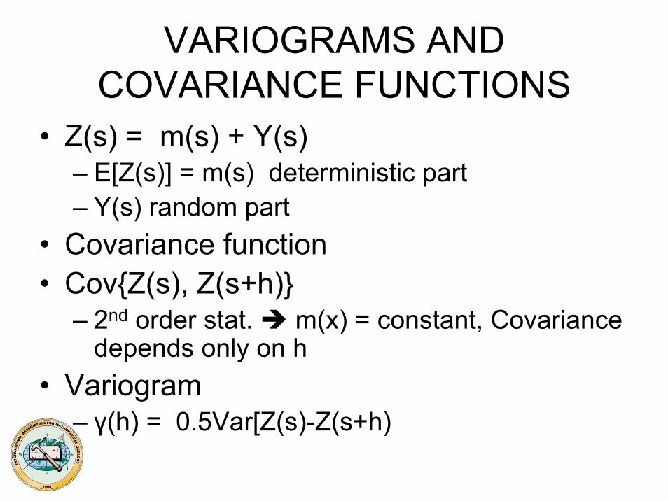
VARIOGRAMS AND COVARIANCE FUNCTIONS
• Z(s) = m(s) + Y(s)– E[Z(s)] = m(s) deterministic part– Y(s) random part
• Covariance function• Cov{Z(s), Z(s+h)}
– 2nd order stat. m(x) = constant, Covariance depends only on h
• Variogram– γ(h) = 0.5Var[Z(s)-Z(s+h)
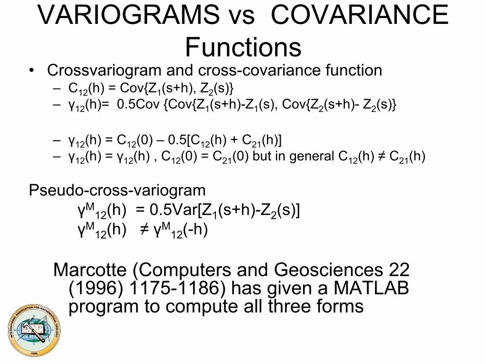
VARIOGRAMS vs COVARIANCE Functions
• Crossvariogram and cross-covariance function– C12(h) = Cov{Z1(s+h), Z2(s)}– γ12(h)= 0.5Cov {Cov{Z1(s+h)-Z1(s), Cov{Z2(s+h)- Z2(s)}
– γ12(h) = C12(0) – 0.5[C12(h) + C21(h)]– γ12(h) = γ12(h) , C12(0) = C21(0) but in general C12(h) ≠ C21(h)
Pseudo-cross-variogramγM
12(h) = 0.5Var[Z1(s+h)-Z2(s)]γM
12(h) ≠ γM12(-h)
Marcotte (Computers and Geosciences 22 (1996) 1175-1186) has given a MATLAB program to compute all three forms
REFERENCES• Clark, I., Basinger, K., and Harper, W.,
1989, MUCK--A Novel Approach to Co-Kriging.
• in B.E. Buxton (Ed.), Proceedings of the Conference on Geostatistical, Sensitivity, and Uncertainty:Methods for Ground-Water Flow and Radionuclide Transport Modeling: Batelle Press,Columbus, p. 473-494.
• Myers, Donald E.,1991, Pseudo-cross variograms, Positive Definiteness and cokriging.
• Mathematical Geology 23, 805-816
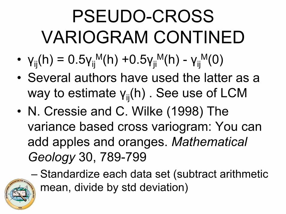
PSEUDO-CROSS VARIOGRAM CONTINED
• γij(h) = 0.5γijM(h) +0.5γji
M(h) - γijM(0)
• Several authors have used the latter as a way to estimate γij(h) . See use of LCM
• N. Cressie and C. Wilke (1998) The variance based cross variogram: You can add apples and oranges. Mathematical Geology 30, 789-799– Standardize each data set (subtract arithmetic
mean, divide by std deviation)
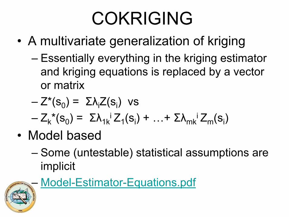
COKRIGING• A multivariate generalization of kriging
– Essentially everything in the kriging estimator and kriging equations is replaced by a vector or matrix
– Z*(s0) = ΣλiZ(si) vs – Zk*(s0) = Σλ1k
i Z1(si) + …+ Σλmki Zm(si)
• Model based – Some (untestable) statistical assumptions are
implicit– Model-Estimator-Equations.pdf
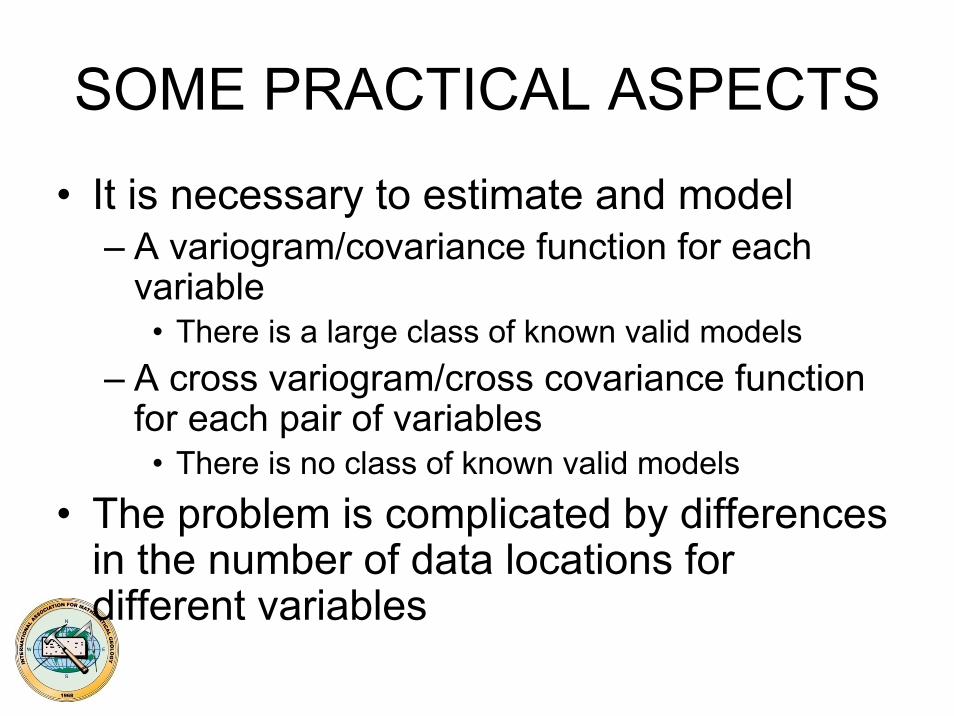
SOME PRACTICAL ASPECTS
• It is necessary to estimate and model – A variogram/covariance function for each
variable• There is a large class of known valid models
– A cross variogram/cross covariance function for each pair of variables
• There is no class of known valid models
• The problem is complicated by differences in the number of data locations for different variables
• The system of equations is larger, greater chance of numerical instability
• Ordinary cokriging assumes that the mean of each random function is constant (with respect to location), estimating the trend is not the same as estimating the mean– The sample variogram only estimates the
variogram is the mean is a constant– In practice one often uses the residuals from
a trend surface or a regression to estimate the variograms. This is sub-optimal
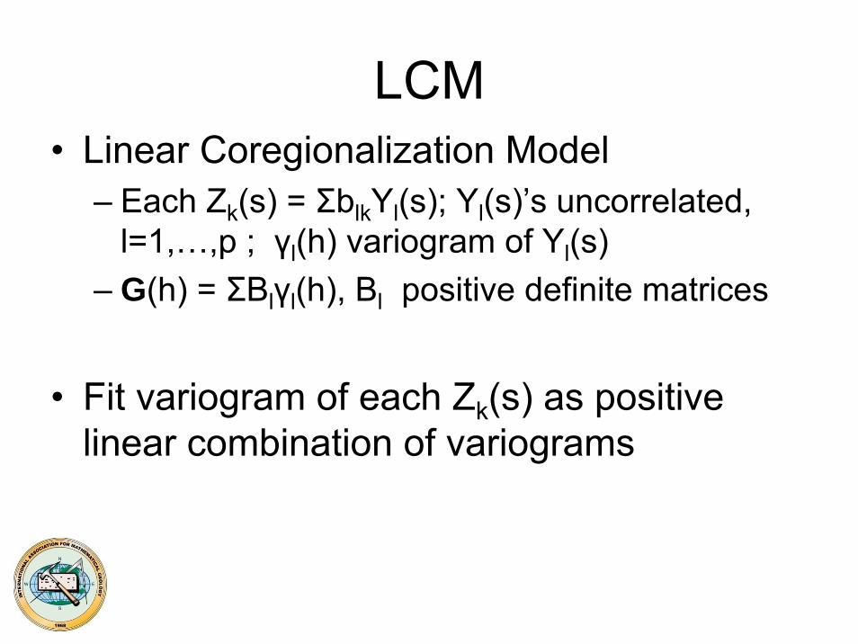
LCM• Linear Coregionalization Model
– Each Zk(s) = ΣblkYl(s); Yl(s)’s uncorrelated, l=1,…,p ; γl(h) variogram of Yl(s)
– G(h) = ΣBlγl(h), Bl positive definite matrices
• Fit variogram of each Zk(s) as positive linear combination of variograms
SOFTWARE• gstat (R package)
• gstat tutorial.pdf• gstat.pdf
– cran.r-project.org/web/packages/gstat/vignettes/gstat.pdf
– cran.r-project.org/web/packages/gstat/gstat.pdf• GSLIB
– FORTRAN codes– pangea.stanford.edu/ERE/research/scrf/software/gslib/help/progr
am/cokb3d.html– www.uofaweb.ualberta.ca/ccg/pdfs/Vol1-IntroCCGSC.pdf
• FAO-Rome– www.enge.ucl.ac.be/recherche/projets/agromet/man0.htm
• SGeMs – http://sgems.sourceforge.net/
• Cokriging with Matlab– Computers & Geosciences 17 (1991) 1265-
1280
MORE ON SOFTWARE
Overview gstat and geoR.pdf
Simplied form of cokriging demo in gstat.pdf
• 1997 A.E. Long and D.E. Myers, A new form of the Cokriging equations. Math. Geology 29, 685-703
SOME EXAMPLES• Precipitation estimation in mountainous terrain
using multivariate geostatistics– J. Applied Meteorology 31 (1992) 661-676 & 677-678
• Cokriging estimation of daily suspended sediment loads – J. Hydrology 327 (2006) 389-398
• A Statistical-Topographical model for mapping climatological precipitation in mountainous terrain – J. of Applied Meteorology 33 (1994) 140-158
MORE EXAMPLES• Flood estimation using radar and rain
gage data. – J. Hydrology 239 (2000) 4-18
• Spatial interpolation of climatic Normals: test of new method in the Canadian boreal forest. – Agric. and Forest Met. 92(1998) 211-225
• Estimating soil water content using cokriging. – Soil Science Soc. Amer. J. 51(1987) 21-30
MORE EXAMPLESRemote sensing based-geostatistical based modeling of forest canopy structure
www.kars.ku.edu/forest/asprs2000_cb.pdf Design of a Low-Boom Supersonic Business Jet Using Cokriging Approximation Models9th AIAA/ISSMO Symposium on Multidisciplinary Analysis and Optimization September 4–6, 2002/Atlanta, GeorgiaAerodynamic Optimization of Rocket Control Surfaces Using Cartesian Methods and CAD Geometry23rd AIAA Applied Aerodynamics Conference, Jun. 6–9, 2005, Toronto, Ontario
Nonlocal problems involving spatial structure for coupledreaction-diffusion systemsApplied Mathematics and Computation 185 (2007) 449-463
MORE EXAMPLES• Application of Cokriging in iron ore
evaluation: Iron ore quadrangle-Brazilin Geostatistics Wollongong ‘96 (eds) E. Baafi
and N. Schofield, Kluwer Academic publishers 1997
• A comparison between cokriging and ordinary kriging: Case study with a polymetallic deposit. Mathematical Geology 25 (2004) 377-398
• 3-D seismic porosity modeling using a new form of cokriging. World Oil May 1999
MORE EXAMPLES
• Climate spatial variability and data resolution in a semi-arid watershed, south-eastern Arizona
Susan M. Skirvin et al (2003) Journal of Arid Environments 54, 667–686
• Cokriging Optimization Of Monitoring Network Configuration Based On Fuzzy And Non-fuzzy Variogram Evaluation – Environmental Monitoring and Assessment 82
(2003) 1-21
MORE EXAMPLES• Detecting and modeling spatial and
temporal dependence in conservation biology – Conservation Biology 14(2000) 1893-1897
• A cokriging method for estimating population density in urban areas.– Computers, Environment and Urban Systems
29 (2005)• Analysis of microarray gene expression
data – Current Bioinformatics 1 (2006) 37-53
SPATIAL-TEMPORAL DATA AND COKRIGING II
• Practical problems with spatial temporal data– More time points than spatial– Not the same spatial locations for different
times– Complicates modeling a spatial temporal
variogram• Treat values at different times as different
variables
SPATIAL-TEMPORAL DATA AND COKRIGING II
• Use cokriging– Use pseudo-cross variogram – Doesn’t allow prediction at intermediate times
• Rouhani, S. and D.E. Myers, D.E. (1990) Problems in Space-Time Kriging of Hydrogeological data. Mathematical Geology, 22, 611-623
Pseudo-cross variogram examples I
Estimation of soil nitrate distributions using cokriging with pseudo-cross variograms
J. Environmental Quality 28 (1999) 424-428Robust estimation of the pseudo-cross variogram for cokriging soil properties
European J. of Soil Science 53 (2002) 253-270
Pseudo-cross variogram examples II
• Ortiz and Emery (J. South African Institute of Mining and Metallurgy 106 (2006) 577-584) use the pseudo-cross variogram to fit an LCM for drill hole and blast hole data for a Porphry copper deposit
• Vanderlinden et al (J. Environmental Quality 35 (2006) 21-36) used the pseudo cross variogram in mapping non-collocated spatial temporal mine spill data
Pseudo-cross variogram examples III
• Geostatistical analysis of stereoscopic pairs of satellite images– In P. Monestiez et al (eds) geoENV III
Environmental Applications of geostatistics (2001)
• Registering two different images of the same terrain
• Lark et al (Geoderma 133 (2006) 363-379) used pseudo cross variograms to map non –collocated spatial temporal soil data
VARIATIONS ON COKRIGING• UNDERSAMPLED CASE
– Most common application– Can be accommodated in the software
• COLLOCATED COKRIGING– Data on secondary variables only at
estimation points• FACTORIAL KRIGING
– Estimate data on Yl(s)’s in LCM• UNIVERSAL COKRIGING or
DETRENDED COKRIGING
ALTERNATIVES CONTINUED
• Which Models for Collocated Cokriging? Jacques Rivoirard (2001) Mathematical Geology 33, 117-131
• Estimating Monthly Streamflow Values by Cokriging . Andrew R. Solow and Steven M. Gorelick (1986) Mathematical Geology 18 , 785-809
FACTORIAL KRIGING EXAMPLES
• Scale Matching with Factorial Kriging for Improved Porosity Estimation from Seismic Data– Math. Geology 31 (1999) 23-46
• FACTOR2D: a computer program for factorial cokriging– Computers & Geosciences 28 (2202) 857-875
COLLOCATED EXAMPLES• Mapping Soil Carbon Using Collocated
Cokriging with Wetness Index – 12th Conference of Int. Association for Mathematical
Geology, Beijing, China, August 26-31, 2007, 391-395
• 3-D Seismic porosity modeling using a new form of cokriging (collocated cokriging)– World Oil 220 (1999) 77-84
ALTERNATIVES TO COKRIGING• KRIGING WITH EXTERNAL DRIFT
– E[Z1(s)] = f(Z2(s)), usually a polynomial• Assumes data for Z2(s) available at estimation points
– Geoadditive Models• J. of the Royal Statistical Society: Series C (Applied
Statistics) 52 (2003)1-18
• KRIGING LINEAR COMBINATIONS– Math.Geology 15 (1983) 633-637
• USE OF PCA TO SEPARATE VARIABLES– Math. Geology 15 (1983) 287-300
EXTERNAL DRIFT EXAMPLES I• Ahmed, S. and de Marsily, G. (1987).
Comparison of geostatistical methods for estimating transmissivity using data on transmissivity and specific capacity. Water Resources Research 23, 1717-1737
• Yates, S. and Warrick, A. W. (1987). `Estimating soil water content using cokriging'. Soil Science Society of
• America Journal 51, 23-30
EXTERNAL DRIFT EXAMPLES II
• Kriging with an external drift versus collocated cokriging for water table mapping – Applied Earth Science (Trans. Inst. Min. Metall. B)
115 (2006) 103-111
• Application of kriging with external drift to estimate hydraulic conductivity from electrical-resistivity data in unconsolidated deposits near Montalto Uffugo, Italy – Hydrogeology J. 8 (2000) 356-367
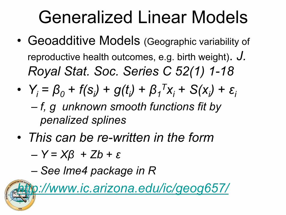
Generalized Linear Models• Geoadditive Models (Geographic variability of
reproductive health outcomes, e.g. birth weight). J. Royal Stat. Soc. Series C 52(1) 1-18
• Yi = β0 + f(si) + g(ti) + β1Txi + S(xi) + εi
– f, g unknown smooth functions fit by penalized splines
• This can be re-written in the form– Y = Xβ + Zb + ε– See lme4 package in R
http://www.ic.arizona.edu/ic/geog657/

IAMG
http://www.iamg.org