multistation methods for geotechnical characterization...

3Chapter 3

Rayleigh Waves

3.1 Overview

Waves that propagate in a medium can be roughly divided into two maincategories: body waves and surface waves. Surface waves are generated only inpresence of a free boundary and they can be essentially of two types: Love wavesand Rayleigh waves. Love waves can exist only in presence of a soft superficiallayer over a stiffer halfspace and they are produced by energy trapping in the softerlayer for multiple reflections. Rayleigh waves are always generated when a freesurface exists in a continuous body.

John Strutt Lord of Rayleigh firstly introduced them as solution of the freevibration problem for an elastic halfspace in 1885 (“On waves propagated alongthe plane surface of an elastic solid”). In the last sentences of the above paper, heanticipated the importance that such kind of wave could have in earthquake tremortransmission. Indeed the introduction of surface waves was preceded by someseismic observations that couldn’t be explained using only body wave theory,which was well known at that time. First of all the nature of the major tremor wasnot clear, because the first arrivals were a couple of minor tremors correspondingto P and S waves respectively. The greater amount of energy associated to this latetremor if compared to that of body wave was a strong evidence of less attenuationpassing through the same medium and this could be explained only assuming thatthis further kind of wave was essentially confined to the surface (Graff 1975).

Another main contribution regarding the forced vibrations was successively

28 Multistation methods for geotechnical characterization using surface waves S.Foti

given by Horace Lamb (“On the propagation of tremors over the surface of anelastic solid”, 1904), who solved the problem of a point harmonic force acting onthe ground surface. He also proposed the solution for the case of a general pulse,by using the Fourier synthesis concept.

Usefulness of surface waves for characterization problems has been soon cleardue to some important features and especially to the possibility of detecting themfrom the surface of a solid, with strong implications on non-invasive techniquesdevelopment (Viktorov 1967).

In this chapter an overview will be given about specific properties of Rayleighwaves, with special aim at soil characterization purposes, leaving morecomprehensive treatment to specific references.

Also some numerical simulations and some experimental data will bepresented in the view of clarifying some important aspects related to Rayleighwaves propagation and to its modelling.

3.2 Homogeneous halfspace

3.2.1 Linear elastic medium

If the free boundary condition is imposed on the general equations for wavepropagation in a linear elastic homogeneous medium, the solution for surfaceRayleigh wave can be deduced from the P-SV components of the wave. It isimportant to note that a SH wave propagating on a free boundary can exist onlyunder restrictive layering condition (and in that case it is usually called Love wave)and hence it cannot exist for the homogeneous halfspace.

The Navier’s equations for dynamical equilibrium in vector formulation canbe expressed as:

ufuu !!44((* '+5+&55+ 2)( (3.1)

where u is the particle displacement vector, 4 the medium density, * and ( theLamè’s constants and f the body forces. Neglecting the latter contribution, the freevibration problem is addressed.

The solution can be searched using Helmholtz decomposition and assumingan exponential form (Richart et Al. 1970). The motivation for assuming theexponential form is that by definition a surface wave must decay quickly withdepth.

Chapter 3 Rayleigh Waves 29

Imposing the boundary conditions of null stress at the free surface:

0ó ' (3.2)

the surface wave solution can be found. In particular for the case of plane strain,discarding the solutions that give infinite amplitude at infinite depth, a solution(Rayleigh wave) can be found only if the following characteristic equation issatisfied by the velocity of propagation of the surface wave:

0)1(16)1624(8 22246 '-&+&-+- ## KKK (3.3)

where K and G are the following ratios between velocities of longitudinal (P),distortional (S) and Rayleigh (R) waves:

S

R

V

VK ' (3.4)

P

S

V

V'# (3.5)

This equation is a cubic on 2K and its roots are a function of Poisson Ratio ,

since, as shown in Paragraph 2.3.1, )1(2

212

,,

#--

' . It can be shown (Viktorov

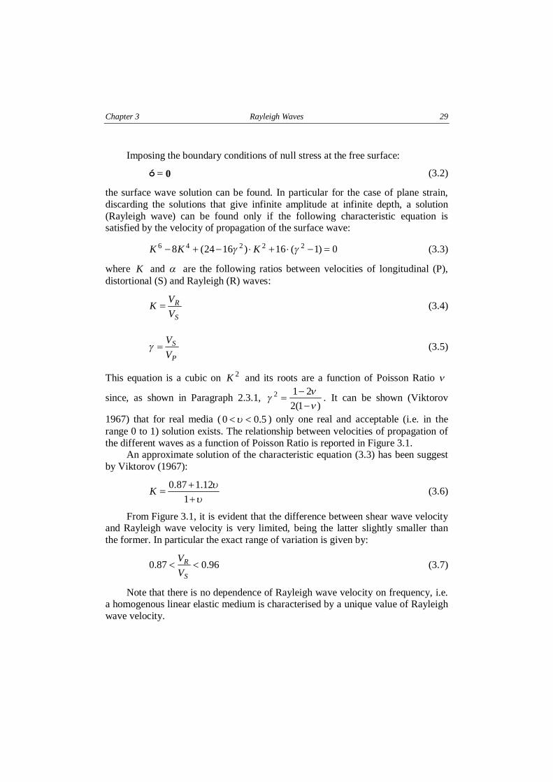
1967) that for real media ( 5.00 PP: ) only one real and acceptable (i.e. in therange 0 to 1) solution exists. The relationship between velocities of propagation ofthe different waves as a function of Poisson Ratio is reported in Figure 3.1.

An approximate solution of the characteristic equation (3.3) has been suggestby Viktorov (1967):

::

++

'1

12.187.0K (3.6)

From Figure 3.1, it is evident that the difference between shear wave velocityand Rayleigh wave velocity is very limited, being the latter slightly smaller thanthe former. In particular the exact range of variation is given by:

96.087.0 PPS

R

V

V(3.7)

Note that there is no dependence of Rayleigh wave velocity on frequency, i.e.a homogenous linear elastic medium is characterised by a unique value of Rayleighwave velocity.


Figure 3.1 Relation between Poisson’s ratio and velocity of propagation ofcompression (P), shear (S) and Rayleigh (R) waves in a linear elastic homogeneoushalfspace (from Richart 1962)

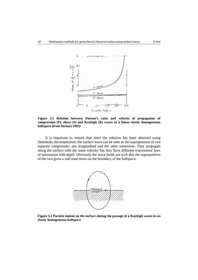
It is important to remark that since the solution has been obtained usingHelmholtz decomposition, the surface wave can be seen as the superposition of twoseparate components: one longitudinal and the other transverse. They propagatealong the surface with the same velocity but they have different exponential lawsof attenuation with depth. Obviously the wave fields are such that the superpositionof the two gives a null total stress on the boundary of the halfspace.

Figure 3.2 Particle motion on the surface during the passage of a Rayleigh waves in anelastic homogeneous halfspace


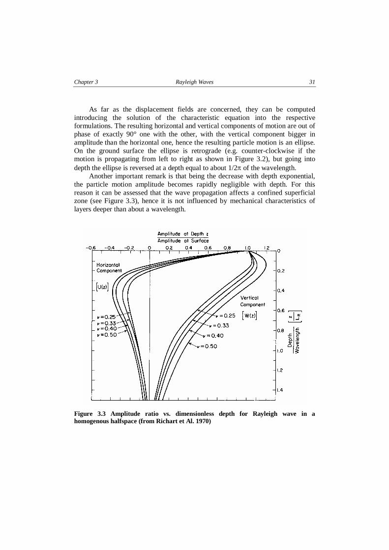
As far as the displacement fields are concerned, they can be computedintroducing the solution of the characteristic equation into the respectiveformulations. The resulting horizontal and vertical components of motion are out ofphase of exactly 90° one with the other, with the vertical component bigger inamplitude than the horizontal one, hence the resulting particle motion is an ellipse.On the ground surface the ellipse is retrograde (e.g. counter-clockwise if themotion is propagating from left to right as shown in Figure 3.2), but going intodepth the ellipse is reversed at a depth equal to about 1/2@ of the wavelength.

Another important remark is that being the decrease with depth exponential,the particle motion amplitude becomes rapidly negligible with depth. For thisreason it can be assessed that the wave propagation affects a confined superficialzone (see Figure 3.3), hence it is not influenced by mechanical characteristics oflayers deeper than about a wavelength.

Figure 3.3 Amplitude ratio vs. dimensionless depth for Rayleigh wave in ahomogenous halfspace (from Richart et Al. 1970)


The solution for a line or point source acting on the ground surface can befound in the Lamb’s paper that has been cited above. In this regard it is importantto remark that, due to the axial-symmetry of the problem, the disturbance spreadsaway in the form of an annular wave field. The reduced geometrical attenuation ofsurface waves can be directly associated to this property.

Also Lord Rayleigh, although he didn’t solve the case of a point source, had asimilar intuition about surface waves: "Diverging in two dimensions only, theymust acquire at a great distance from the source a continually increasingpreponderance" (concluding remarks of the above cited paper).

The geometric spreading factor, i.e. the factor according to which the wavesattenuate as they go away from the source, can be estimate with the followingphysical considerations about the wave fronts.

Considering a buried point source in an infinite medium, the released energyspreads over a spherical surface and hence its attenuation is proportional to thesquare of distance from the source. Since the energy is proportional to the square ofdisplacements, the latter ones attenuate proportionally to distance. Analogouslysince Rayleigh waves, that are generated by a point source acting on the groundsurface, propagate with a cylindrical wave-front, their energy attenuation must beproportional to distance and displacement attenuation to the square root of distance.Concerning the geometrical attenuation of longitudinal and shear waves along thefree surface, it is not possible an analogy to previous cases, but it can be shown thatbecause of leaking of energy into the free space the displacement attenuation goeswith the square of distance (Richart et al. 1970). In summary for a linear elastichalfspace a simple power law of the following type can express the radiationdamping consequences on waves amplitude:

QQ

R

QQ

S

T

'

wavesRayleighfor2

1

solidtheintowavesbodyfor1

surfacetheonwavesshearandallongitudinfor2

with1

nr n

(3.8)

where r is the distance from the point source.Back to Lamb’s work, the displacements at great distance r from a vertical

harmonic point force tiz eF 3& can be expressed as:


ABC

DEF --

&&' 4

@3 krti

zzz e

r

bFu (3.9)

ABC

DEF +-

&&' 4

@3 krti

rzr e

r

bFu (3.10)

where zu and ru are the vertical and radial displacements, zb and rb are

functions of the mechanical parameters of the medium and k is the wavenumberthat is defined by the following relation:

RVk

3' (3.11)

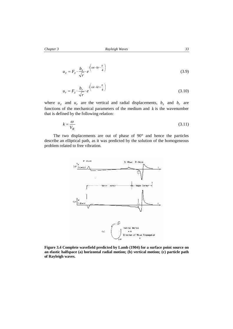
The two displacements are out of phase of 90° and hence the particlesdescribe an elliptical path, as it was predicted by the solution of the homogeneousproblem related to free vibration.

Figure 3.4 Complete wavefield predicted by Lamb (1904) for a surface point source onan elastic halfspace (a) horizontal radial motion; (b) vertical motion; (c) particle pathof Rayleigh waves.


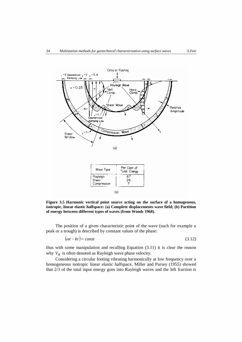
Figure 3.5 Harmonic vertical point source acting on the surface of a homogenous,isotropic, linear elastic halfspace: (a) Complete displacements wave field; (b) Partitionof energy between different types of waves (from Woods 1968).

The position of a given characteristic point of the wave (such for example apeak or a trough) is described by constant values of the phase:

/ 0 constkrt '-3 (3.12)

thus with some manipulation and recalling Equation (3.11) it is clear the reasonwhy RV is often denoted as Rayleigh wave phase velocity.

Considering a circular footing vibrating harmonically at low frequency over ahomogeneous isotropic linear elastic halfspace, Miller and Pursey (1955) showedthat 2/3 of the total input energy goes into Rayleigh waves and the left fraction is


divided between body waves (see Figure 3.5b). Adding this information to theabove considerations about geometrical attenuation, the conclusion is that at acertain distance from the source the wavefield is essentially dominated by theRayleigh waves. This is essentially the same conclusion reached by Lamb (1904),who divided the wave contributions in two minor tremors (P and S) and a majortremor (R) (Figure 3.4).

All the important features of the complete wave-field generated by a lowfrequency harmonic point source are summarised in Figure 3.5.

3.2.2 Linear viscoelastic medium

As seen in Chapter 2, also at very low strain levels soil behaviour can’t beconsidered elastic, indeed cycles of loading and unloading show energy dissipation.Recalling the actual nature of soil, it is intuitive that dissipation is essentially due tothe friction between particles and the motion of the pore fluid, and hence it occursalso for very small strains, when the soil is far from the plasticity conditions.

To account for dissipation, an equivalent linear viscoelastic model can beassumed at small strains. In this regard the correspondence principle can be used toextend the result obtained in the case of a linear elastic medium. According to it,the velocity of propagation of seismic waves can be substituted by a complexvalued velocity that accounts for the attenuation of such waves. Adopting thisprinciple Viktorov (1967) showed that the attenuation of surface waves in ahomogeneous linear viscoelastic medium is governed primarily by the shear waveattenuation factor. In particular he found that the Rayleigh wave attenuation RGcould be expressed as a linear combination of the longitudinal wave attenuation

PG and the shear wave attenuation SG , according to the expression:

/ 0 SPR AA GGG &-+&' 1 (3.13)

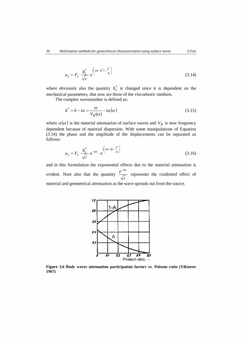
where is A a quantity depending only on the Poisson Ratio. Since A is alwayssmaller than 5.0 , the shear wave attenuation is prevalent in determining theRayleigh wave attenuation. Moreover for Poisson Ratio values higher than 0.2, Ais less than 2.0 (see Figure 3.6).

The wave field generated by a vertical harmonic point source acting on theground surface can be obtained applying the correspondence principle to theLamb’s solution. For example substituting a complex wavenumber in (3.9) it ispossible to evaluate the vertical displacements as:


AB

CDE

F --&&' 4

* * @3 rkti

zzz e

r

bFu (3.14)

where obviously also the quantity *zb is changed since it is dependent on the

mechanical parameters, that now are those of the viscoelastic medium.The complex wavenumber is defined as:

/ 03G33

G iV

ikkR

-'-')(

* (3.15)

where / 03G is the material attenuation of surface waves and RV is now frequencydependent because of material dispersion. With some manipulations of Equation(3.14) the phase and the amplitude of the displacements can be separated asfollows:

ABC

DEF --

- &&&' 4*

@3

Gkrti

rzzz ee

r

bFu (3.16)

and in this formulation the exponential effects due to the material attenuation is

evident. Note also that the quantity r

e rG- represents the combined effect of

material and geometrical attenuation as the wave spreads out from the source.

Figure 3.6 Body waves attenuation participation factors vs. Poisson ratio (Viktorov1967)


3.3 Vertically heterogeneous media

3.3.1 Linear elastic medium

For heterogeneous and anisotropic media the mathematical formulation ofRayleigh waves becomes very complex and there can be cases of anisotropic mediawhere they do not exist at all. However in the case of transverse isotropic mediumwith the free surface parallel to the isotropy plane (common situation for soilsystems) Rayleigh waves exist and the analogous of the Lamb solution can befound (Butchwald 1961).

As far as heterogeneity is concerned, when the mechanical properties of themedium are assumed to be dependent only on depth z , the formal expression ofthe Navier’s equations, neglecting body force, is:

uu

ue.ueu.u !!4(*

((* 'ABC

DEF

>>&+757+5+5+55+

zdz

d

dz

dzz 2)( 2 (3.17)

where ze is the base vector for the direction perpendicular to the free surface.Lai (1998) has showed that introducing in (3.17) the condition of plane strain

(that causes no loss of generality) and assuming the classical exponential form forthe solution, the final solution is given by a linear differential eigenvalue problem.Assuming the usual boundary condition of null stress at the surface, theeigenvalues )(3k can be found as the values that makes equal to zero the

equivalent of the Rayleigh characteristic equation, that in this case can only bewritten in implicit form (Lai 1998):

/ 0 / 0 / 08 9 0,,,,R '34(* jkzzzF (3.18)

It is noteworthy to remark some important features of this equation. First ofall the dependence on the frequency means that also the relative solution will befrequency dependant and hence the resulting wave field is dispersive, meaning thatits phase velocity will be a function of frequency. This dispersion is related to thegeometrical variations of Lamé’s parameters and density with depth and hence it isoften called geometric dispersion. The equation (3.18) itself is often nameddispersion equation.

For a given frequency the solutions of the dispersion equation are severalwhile in the case of the homogeneous halfspace there was only one admissiblesolution of the characteristic equation. This means that many modes of propagationof the Rayleigh wave exist and the solution of the forced vibration case mustaccount for them with a process of mode superposition.


Substituting each one of the eigenvalues (wavenumbers) in the eigenproblemformulation, four eigenfunctions can be retrieved. They correspond to the twodisplacements and the two stresses associated to that particular wave propagationmode.

The existence of several mode of propagation can be explained physicallythrough the concept of constructive interference (Lai 1998).

3.3.1.1 Mathematical formulations for layered media

In the formulation of the dispersion equation (3.18) there was no explicit referenceto any law of variation of the mechanical properties with depth. The problem canbe solved once a law of variation is specified. In general it is not possible to solvethe problem analytically and a numerical solution is needed.

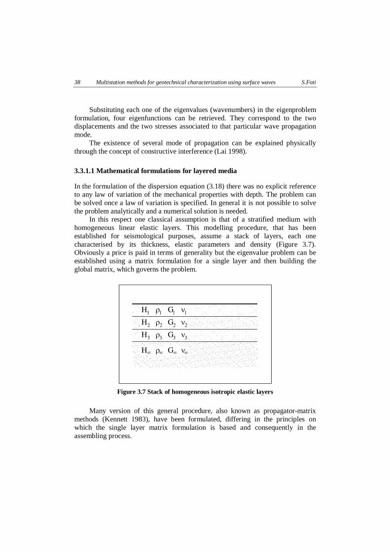
In this respect one classical assumption is that of a stratified medium withhomogeneous linear elastic layers. This modelling procedure, that has beenestablished for seismological purposes, assume a stack of layers, each onecharacterised by its thickness, elastic parameters and density (Figure 3.7).Obviously a price is paid in terms of generality but the eigenvalue problem can beestablished using a matrix formulation for a single layer and then building theglobal matrix, which governs the problem.

Figure 3.7 Stack of homogeneous isotropic elastic layers

Many version of this general procedure, also known as propagator-matrixmethods (Kennett 1983), have been formulated, differing in the principles onwhich the single layer matrix formulation is based and consequently in theassembling process.


The oldest and probably the most famous method is the Transfer-Matrixmethod, originally proposed by Thomson (1950) and successively modified byHaskell (1953).

The Stiffness-Matrix method proposed by Kausel and Roesset (1981) isessentially a reformulation of the Transfer-Matrix method, having the advantage ofa simplified procedure for the assembly of the global matrix, according to theclassical scheme of structural analysis.

The third possibility is given by the construction of reflection andtransmission matrices, which account for the partition of energy as the wave ispropagating. The wave field is then given by the constructive interference of wavestravelling from a layer to another (Kennett 1974, 1979; Kerry 1981).

Once the dispersion equation has been constructed using one of the abovemethods, the successive and very computationally intensive step is the use of a rootsearching technique to obtain the eigenvalues of the problem. Great attention mustbe paid in this process because of the behaviour of the dispersion function. Indeedsome solution searching techniques can easily fail due to the strong oscillations ofthe dispersion function especially at high frequencies (Hisada 1994, 1995). In thisrespect since these methods are borrowed from seismology, the frequenciesinvolved in the soil characterization methods have to be considered high.

Recalling the starting point of the above considerations (Equation (3.17)) theeigenvalues, and hence the correspondent eigenfunctions, that have been computedare the solution of the homogeneous problem, i.e. in absence of an external source.The obtained modes constitute the solution of the free Rayleigh oscillations of theconsidered medium.

If a source exists, the correspondent inhomogeneous problem must be solved.In this case a term that represents the external force is included in Equation (3.17).The solution comes from a mode superposition process. Sometimes this problem isaddressed as the three dimensional solution because waves spread out from thesource following a 3D axial-symmetric path, whereas the free modes representplane waves and hence are addressed as the solution of the 2D problem.

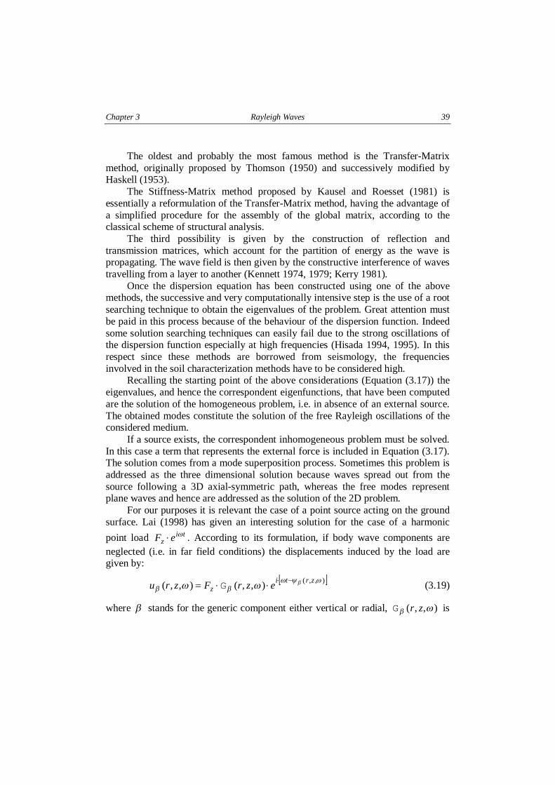
For our purposes it is relevant the case of a point source acting on the groundsurface. Lai (1998) has given an interesting solution for the case of a harmonic

point load tiz eF 3& . According to its formulation, if body wave components are

neglected (i.e. in far field conditions) the displacements induced by the load aregiven by:

8 9),,(),,(),,(

3U3VV

V33 zrtiz ezrFzru

-&&&' G (3.19)

where V stands for the generic component either vertical or radial, ),,( 3V zrG is


the Rayleigh geometrical spreading function, that models the geometric attenuationin layered medium, and ),,( 3U V zr is a composite phase function.

An interesting comparison can be made between Equation (3.19) and itsequivalent for a homogeneous halfspace (Eq. (3.9) and (3.10)), in which case themode of propagation was only one. First of all the geometric attenuation for thehomogeneous halfspace is much simpler. On the other side phase velocity iscoincident with that of the only one mode of propagation, while in the case of thelayered medium also the phase velocity comes from mode superposition and forthis reason is often indicated as effective or apparent phase velocity.

In analogy to Equation (3.12), the position of a given characteristic point ofthe harmonic wave (such for example a peak or a trough) is described by constantvalues of the phase:

/ 0 constzrt '- ),,( 3U3 V (3.20)

hence differentiating with respect to time, under the hypothesis that the function),,( 3U V zr be smooth enough, it is possible to obtain the effective phase velocity

RV̂ (Lai 1998):

r

zrzrVR

>

>'

),,(),,(ˆ

3U3

3V

(3.21)

It is very important to note that since the effective Rayleigh velocity is a functionnot only of frequency but also of the distance from the source, it is a local quantity(see Lai 1998 for a comprehensive discussion on this topic).

3.3.1.2 Physical remarks

Some physical aspects are implicitly included in the mathematical formulations ofvertically heterogeneous media described above. It can be useful trying to describethem in a more phenomenological way.

First of all the geometrical dispersion, i.e. the dependence of Rayleigh phasevelocity on frequency can be easily explained recalling the characteristics ofshallowness of this waves. As exposed in Paragraph 3.2.1 for a homogeneouslinear elastic halfspace the exponential decay of particle motion with depth is suchthat the portion of the medium that is affected by the wave propagation is equal toabout one wavelength. Since the wavelength R* is related to the frequency f bythe following relation:


f

VRR '* (3.22)

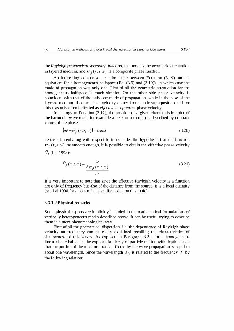
it is clear that low frequency waves will penetrate more into the ground surface.Hence in the case of a vertically heterogeneous medium, surface waves at differentfrequency will involve in their propagation different layers and consequently thephase velocity will be related to a combination of their mechanical properties.Consequently the surface waves velocity will be a function of frequency. Theabove concept is summarised in Figure 3.8, where the vertical displacements wavefield in depth at two different frequencies is presented for a layered medium.

Figure 3.8 Geometrical dispersion in layered media (from Rix 1988)

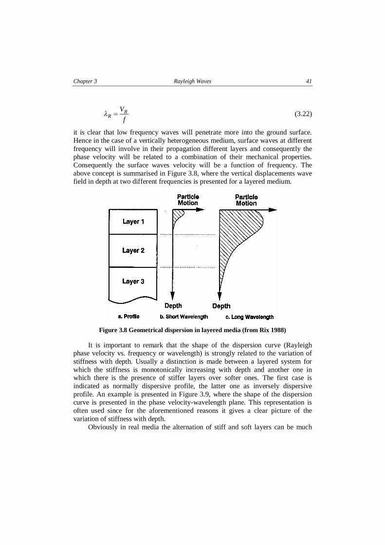
It is important to remark that the shape of the dispersion curve (Rayleighphase velocity vs. frequency or wavelength) is strongly related to the variation ofstiffness with depth. Usually a distinction is made between a layered system forwhich the stiffness is monotonically increasing with depth and another one inwhich there is the presence of stiffer layers over softer ones. The first case isindicated as normally dispersive profile, the latter one as inversely dispersiveprofile. An example is presented in Figure 3.9, where the shape of the dispersioncurve is presented in the phase velocity-wavelength plane. This representation isoften used since for the aforementioned reasons it gives a clear picture of thevariation of stiffness with depth.

Obviously in real media the alternation of stiff and soft layers can be much


more complex if compared to the above cases, still Figure 3.8 gives an idea of therelation existing between the stiffness profile and the dispersion curve.

Figure 3.9 Examples of non dispersive (homogeneous halfspace), normally dispersiveand inversely dispersive profiles (from Rix 1988)


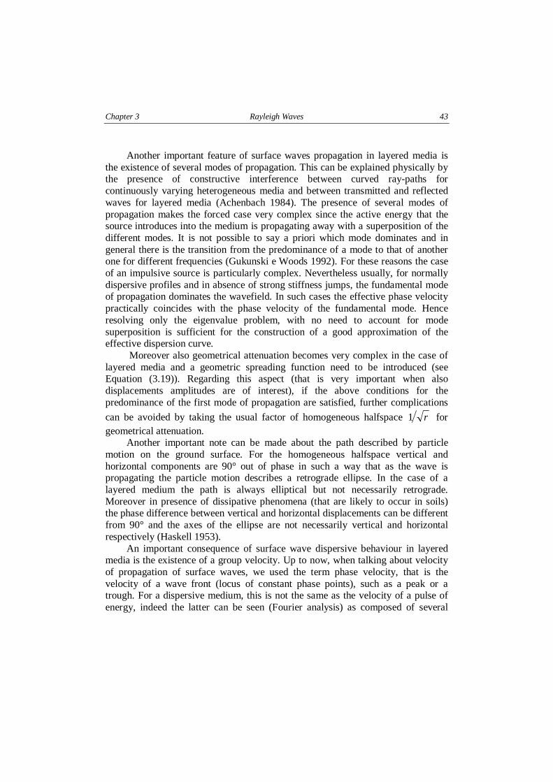
Another important feature of surface waves propagation in layered media isthe existence of several modes of propagation. This can be explained physically bythe presence of constructive interference between curved ray-paths forcontinuously varying heterogeneous media and between transmitted and reflectedwaves for layered media (Achenbach 1984). The presence of several modes ofpropagation makes the forced case very complex since the active energy that thesource introduces into the medium is propagating away with a superposition of thedifferent modes. It is not possible to say a priori which mode dominates and ingeneral there is the transition from the predominance of a mode to that of anotherone for different frequencies (Gukunski e Woods 1992). For these reasons the caseof an impulsive source is particularly complex. Nevertheless usually, for normallydispersive profiles and in absence of strong stiffness jumps, the fundamental modeof propagation dominates the wavefield. In such cases the effective phase velocitypractically coincides with the phase velocity of the fundamental mode. Henceresolving only the eigenvalue problem, with no need to account for modesuperposition is sufficient for the construction of a good approximation of theeffective dispersion curve.

Moreover also geometrical attenuation becomes very complex in the case oflayered media and a geometric spreading function need to be introduced (seeEquation (3.19)). Regarding this aspect (that is very important when alsodisplacements amplitudes are of interest), if the above conditions for thepredominance of the first mode of propagation are satisfied, further complications

can be avoided by taking the usual factor of homogeneous halfspace r1 forgeometrical attenuation.

Another important note can be made about the path described by particlemotion on the ground surface. For the homogeneous halfspace vertical andhorizontal components are 90° out of phase in such a way that as the wave ispropagating the particle motion describes a retrograde ellipse. In the case of alayered medium the path is always elliptical but not necessarily retrograde.Moreover in presence of dissipative phenomena (that are likely to occur in soils)the phase difference between vertical and horizontal displacements can be differentfrom 90° and the axes of the ellipse are not necessarily vertical and horizontalrespectively (Haskell 1953).

An important consequence of surface wave dispersive behaviour in layeredmedia is the existence of a group velocity. Up to now, when talking about velocityof propagation of surface waves, we used the term phase velocity, that is thevelocity of a wave front (locus of constant phase points), such as a peak or atrough. For a dispersive medium, this is not the same as the velocity of a pulse ofenergy, indeed the latter can be seen (Fourier analysis) as composed of several


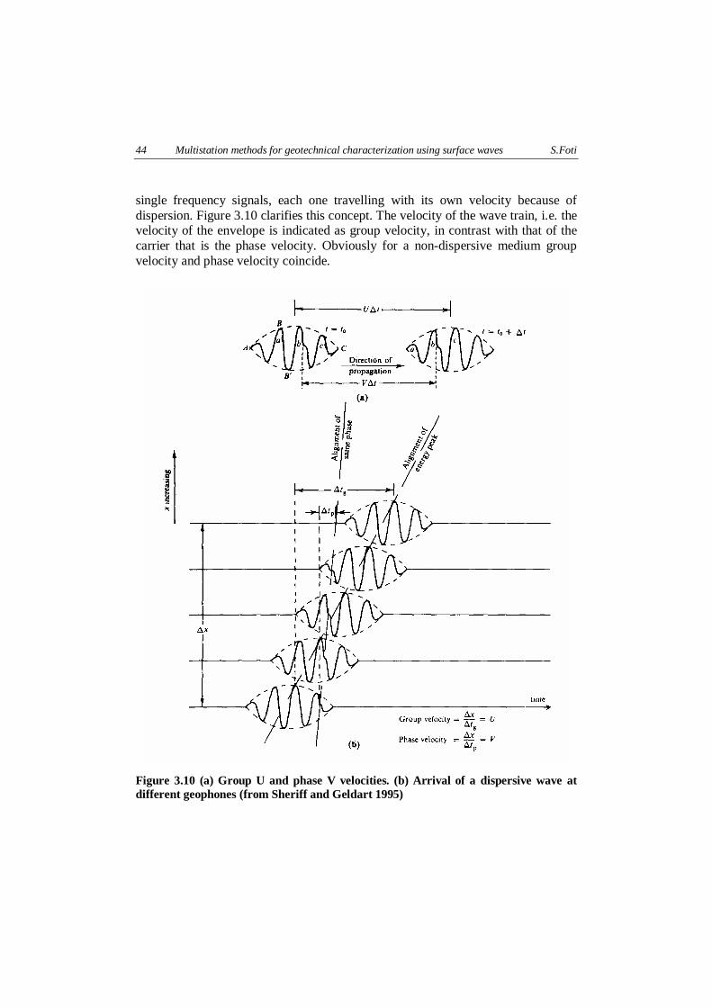
single frequency signals, each one travelling with its own velocity because ofdispersion. Figure 3.10 clarifies this concept. The velocity of the wave train, i.e. thevelocity of the envelope is indicated as group velocity, in contrast with that of thecarrier that is the phase velocity. Obviously for a non-dispersive medium groupvelocity and phase velocity coincide.

Figure 3.10 (a) Group U and phase V velocities. (b) Arrival of a dispersive wave atdifferent geophones (from Sheriff and Geldart 1995)


The group velocity U can be computed using the following expressions,which involve the derivative of phase velocity with respect to frequency f or to

wavelength * (Sheriff and Geldart 1995):

/ 0 **

33

d

dVV

df

dVfV

dk

dU -'+O' (3.23)

where all the values are the average ones over the dominant frequency range.From the above expression it is clear that if modal phase velocity decrease

with increasing frequency (normally dispersive profiles), V is greater than U andhence the carrier travels faster than the envelope. Thus in such cases if a phasedisturbance appears at the beginning of the pulse, then it overtakes and finally itdisappears in the front (as shown in Figure 3.10). Obviously everything reversesfor the case of an inversely dispersive profile.

3.3.2 Linear viscoelastic medium

It is important to distinguish two different cases: one is that of the weaklydissipative medium, the other one is the more general case were no assumption ismade on the magnitude of the dissipation (Lai 1998).

For weakly dissipative media the solution can be obtained directly from thesolution of the linear elastic eigenvalue problem substituting in the relevantexpressions the real elastic phase velocities of body waves with the correspondentcomplex values:

8 98 9SSS

PPP

iDVV

iDVV

-&'

-&'

1)()(

1)()(*

*

33

33(3.24)

where PD and SD are the damping ratios.Instead in the general case the correspondence principle has to be applied to

the formulation of the eigenvalue problem, so that it becomes a complexeigenvalue problem and its solution is not trivial. A solution based on thegeneralisation of the transmission and reflection matrix techniques and appropriateroot searching for complex dispersion equation can be found in Lai (1998). Anexpression, which is formally analogous to Equation (3.19), can be established forthe displacement field generated by a harmonic point source:

8 9),,(*

),,(),,(3U3

VVV33 zrti

vzvezrFzru

-&&&' G (3.25)


where ),,(),,( 33 VV zrzrv GG W is the geometric spreading function for the

layered viscoelastic medium and the function ),,(*

3U V zrv in the exponent is now

complex-valued.In relation to what exposed in Paragraph 3.3.1.2, it is important to recall that

in the case of a viscoelastic layered medium, material dispersion is added togeometrical dispersion, hence the phenomenon is more complex, with respect tothe way in which it was explained for layered elastic media.

3.4 Numerical examples

Some numerical simulations regarding the case of linear elastic stratified mediumare presented hereafter. The results have been obtained using a freeware computerprogram developed by Hisada and modified formerly by Lai (1998) andsuccessively by the Author. The construction of the eigenvalue problem is based onthe formulation of transmission and reflection matrices, initially proposed byKennet (1975) and successively modified with the contribution of severalresearches (Luco and Apsel 1983, Apsel and Luco 1983, Chen 1993). The relativetheory can be found in Hisada (1994, 1995).

The basic purpose of these numerical simulations is to illustrate some basicfeatures of Rayleigh waves in vertically heterogeneous media, that have beendelineated in the theory above.

Two stiffness profiles are considered to show the differences betweennormally dispersive and inversely dispersive media. This difference has a hugeinfluence on characterization problems, because the presence of stiff layers oversofter ones produces the shift of the dominating mode from the fundamental onetowards the higher ones.

3.4.1 Normally dispersive profile

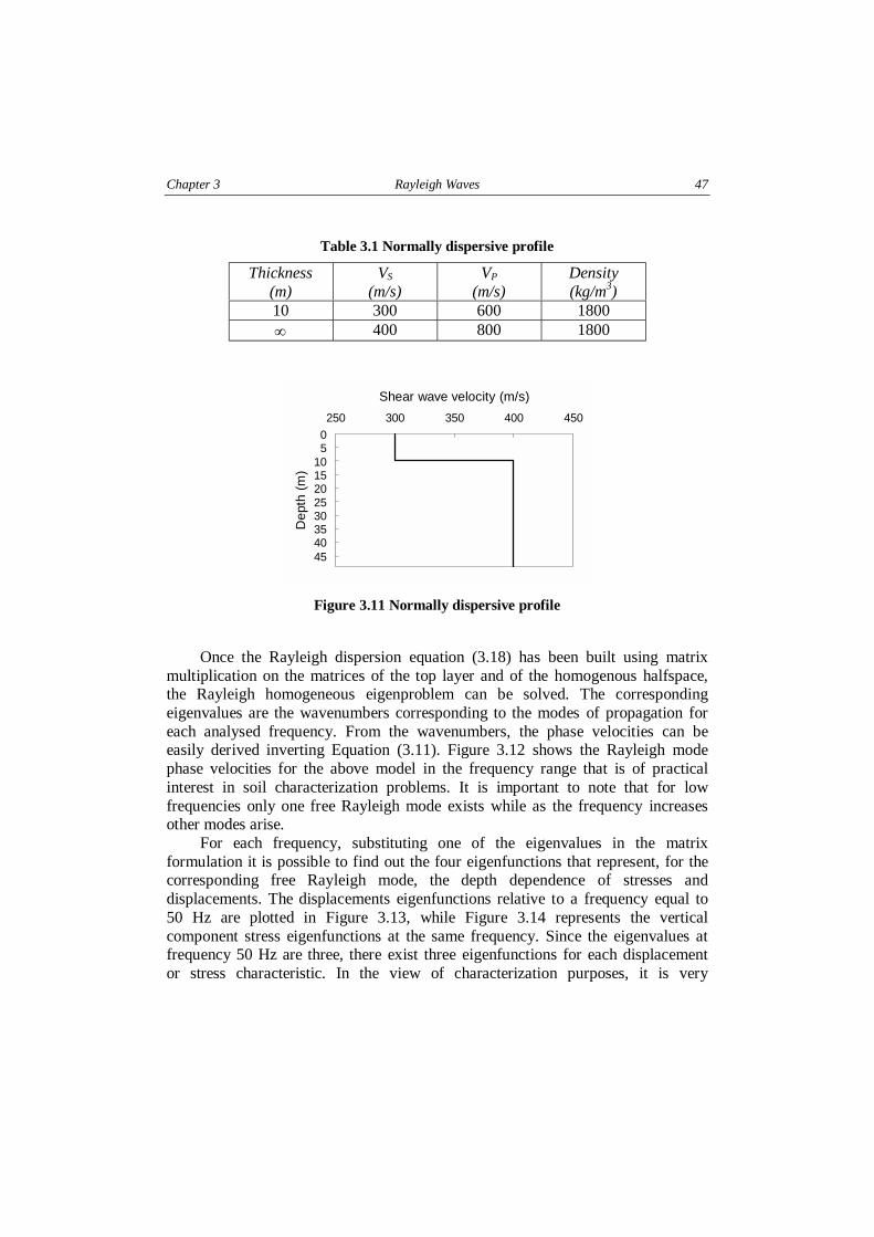
Firstly the very simple case of a layer over a homogeneous halfspace is considered.The model parameters are reported in Table 3.1. They are such that the medium isnormally dispersive, the stiffness being monotonically increasing with depth.


Table 3.1 Normally dispersive profile

Thickness(m)

VS

(m/s)VP

(m/s)Density(kg/m3)

10 300 600 18002 400 800 1800

05

1015202530354045

250 300 350 400 450

Shear wave velocity (m/s)

De

pth

(m

)

Figure 3.11 Normally dispersive profile

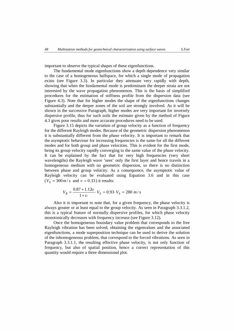
Once the Rayleigh dispersion equation (3.18) has been built using matrixmultiplication on the matrices of the top layer and of the homogenous halfspace,the Rayleigh homogeneous eigenproblem can be solved. The correspondingeigenvalues are the wavenumbers corresponding to the modes of propagation foreach analysed frequency. From the wavenumbers, the phase velocities can beeasily derived inverting Equation (3.11). Figure 3.12 shows the Rayleigh modephase velocities for the above model in the frequency range that is of practicalinterest in soil characterization problems. It is important to note that for lowfrequencies only one free Rayleigh mode exists while as the frequency increasesother modes arise.

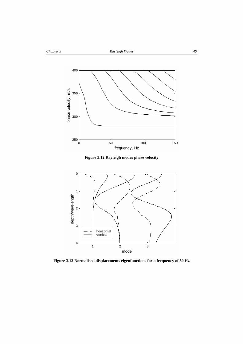
For each frequency, substituting one of the eigenvalues in the matrixformulation it is possible to find out the four eigenfunctions that represent, for thecorresponding free Rayleigh mode, the depth dependence of stresses anddisplacements. The displacements eigenfunctions relative to a frequency equal to50 Hz are plotted in Figure 3.13, while Figure 3.14 represents the verticalcomponent stress eigenfunctions at the same frequency. Since the eigenvalues atfrequency 50 Hz are three, there exist three eigenfunctions for each displacementor stress characteristic. In the view of characterization purposes, it is very


important to observe the typical shapes of these eigenfunctions.The fundamental mode eigenfunctions show a depth dependence very similar

to the case of a homogeneous halfspace, for which a single mode of propagationexists (see Figure 3.3). In particular they attenuate very rapidly with depth,showing that when the fundamental mode is predominant the deeper strata are notinterested by the wave propagation phenomenon. This is the basis of simplifiedprocedures for the estimation of stiffness profile from the dispersion data (seeFigure 4.3). Note that for higher modes the shape of the eigenfunctions changessubstantially and the deeper zones of the soil are strongly involved. As it will beshown in the successive Paragraph, higher modes are very important for inverselydispersive profile, thus for such soils the estimate given by the method of Figure4.3 gives poor results and more accurate procedures need to be used.

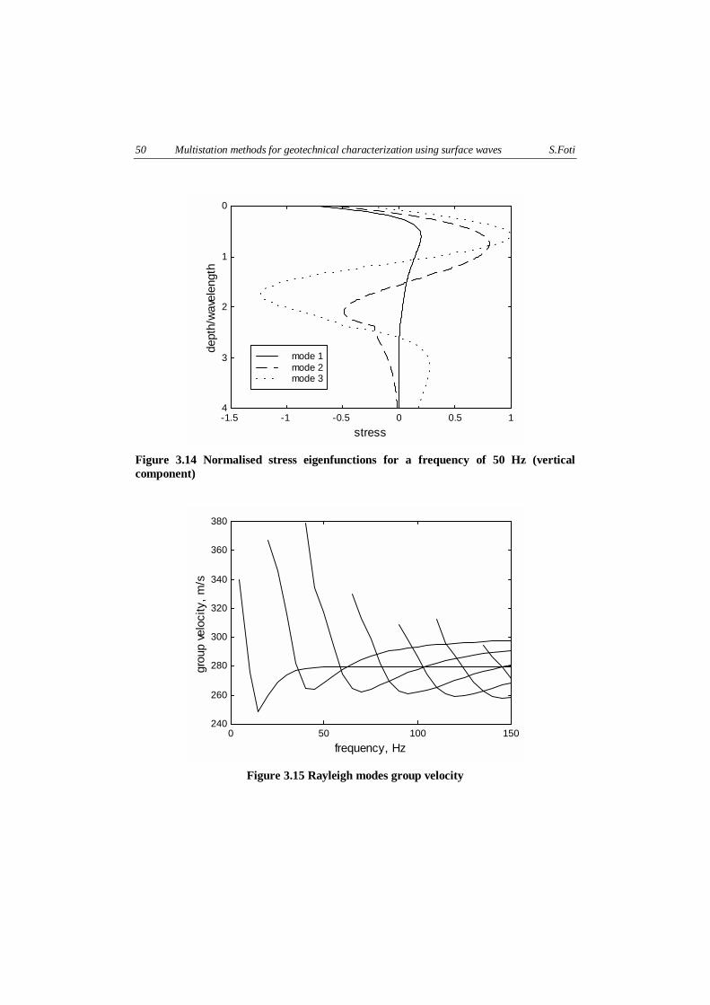
Figure 3.15 depicts the variation of group velocity as a function of frequencyfor the different Rayleigh modes. Because of the geometric dispersion phenomenonit is substantially different from the phase velocity. It is important to remark thatthe asymptotic behaviour for increasing frequencies is the same for all the differentmodes and for both group and phase velocities. This is evident for the first mode,being its group velocity rapidly converging to the same value of the phase velocity.It can be explained by the fact that for very high frequencies (very shortwavelengths) the Rayleigh wave ’sees’ only the first layer and hence travels in ahomogeneous medium with no geometric dispersion, so there is no distinctionbetween phase and group velocity. As a consequence, the asymptotic value ofRayleigh velocity can be evaluated using Equation 3.6 and in this case( smVS /300' and 33.0', ) it results:

smVVV SSR /28093.01

12.187.0 '&'&++

':

:

Also it is important to note that, for a given frequency, the phase velocity isalways greater or at least equal to the group velocity. As seen in Paragraph 3.3.1.2,this is a typical feature of normally dispersive profiles, for which phase velocitymonotonically decreases with frequency increase (see Figure 3.12).

Once the homogeneous boundary value problem that corresponds to the freeRayleigh vibration has been solved, obtaining the eigenvalues and the associatedeigenfunctions, a mode superposition technique can be used to derive the solutionof the inhomogeneous problem, that correspond to the forced vibrations. As seen inParagraph 3.3.1.1, the resulting effective phase velocity, is not only function offrequency, but also of spatial position, hence a correct representation of thisquantity would require a three dimensional plot.


0 50 100 150250

300

350

400

frequency, Hz

phas

e ve

loci

ty,

m/s

Figure 3.12 Rayleigh modes phase velocity

1 2 3

0

1

2

3

4

mode

dept

h/w

avel

engt

h

horizontalvertical

Figure 3.13 Normalised displacements eigenfunctions for a frequency of 50 Hz


-1.5 -1 -0.5 0 0.5 1

0

1

2

3

4

stress

dept

h/w

avel

engt

h

mode 1mode 2mode 3

Figure 3.14 Normalised stress eigenfunctions for a frequency of 50 Hz (verticalcomponent)

0 50 100 150240

260

280

300

320

340

360

380

frequency, Hz

grou

p ve

loci

ty,

m/s

Figure 3.15 Rayleigh modes group velocity


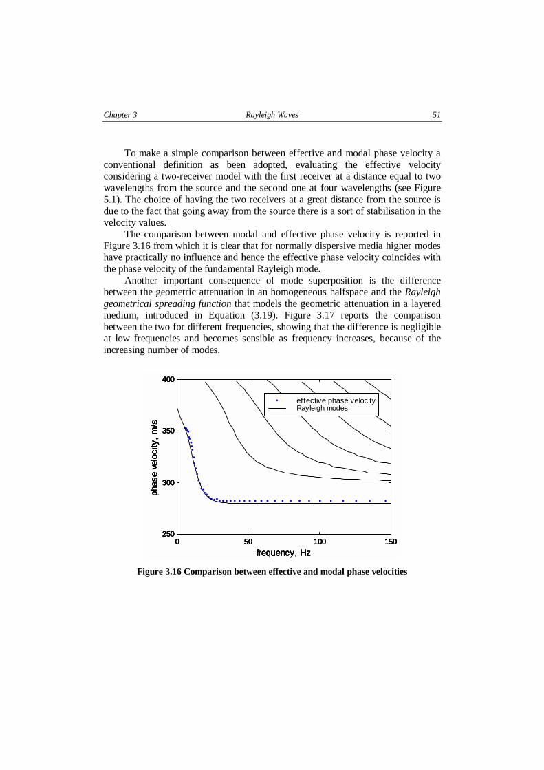
To make a simple comparison between effective and modal phase velocity aconventional definition as been adopted, evaluating the effective velocityconsidering a two-receiver model with the first receiver at a distance equal to twowavelengths from the source and the second one at four wavelengths (see Figure5.1). The choice of having the two receivers at a great distance from the source isdue to the fact that going away from the source there is a sort of stabilisation in thevelocity values.

The comparison between modal and effective phase velocity is reported inFigure 3.16 from which it is clear that for normally dispersive media higher modeshave practically no influence and hence the effective phase velocity coincides withthe phase velocity of the fundamental Rayleigh mode.

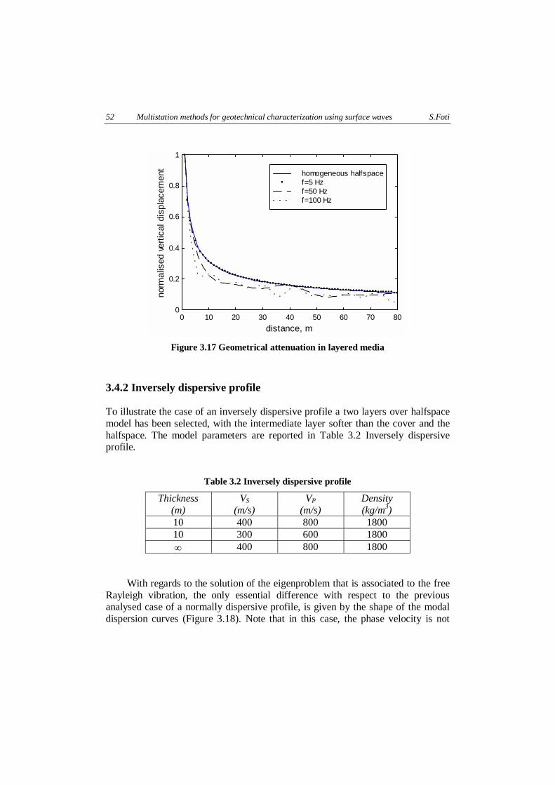
Another important consequence of mode superposition is the differencebetween the geometric attenuation in an homogeneous halfspace and the Rayleighgeometrical spreading function that models the geometric attenuation in a layeredmedium, introduced in Equation (3.19). Figure 3.17 reports the comparisonbetween the two for different frequencies, showing that the difference is negligibleat low frequencies and becomes sensible as frequency increases, because of theincreasing number of modes.

0 50 100 150250

300

350

400

frequency, Hz

phas

e ve

loci

ty,

m/s

effective phase velocityRayleigh modes

0 50 100 150250

300

350

400

frequency, Hz

phas

e ve

loci

ty,

m/s


0 50 100 150250

300

350

400

frequency, Hz

phas

e ve

loci

ty,

m/s

0 50 100 150250

300

350

400

frequency, Hz

phas

e ve

loci

ty,

m/s


Figure 3.16 Comparison between effective and modal phase velocities


0 10 20 30 40 50 60 70 800

0.2

0.4

0.6

0.8

1

distance, m

norm

alis

ed v

ertic

al d

ispl

acem

ent

homogeneous halfspacef=5 Hzf=50 Hzf=100 Hz

Figure 3.17 Geometrical attenuation in layered media

3.4.2 Inversely dispersive profile

To illustrate the case of an inversely dispersive profile a two layers over halfspacemodel has been selected, with the intermediate layer softer than the cover and thehalfspace. The model parameters are reported in Table 3.2 Inversely dispersiveprofile.

Table 3.2 Inversely dispersive profile

Thickness(m)

VS

(m/s)VP

(m/s)Density(kg/m3)

10 400 800 180010 300 600 18002 400 800 1800

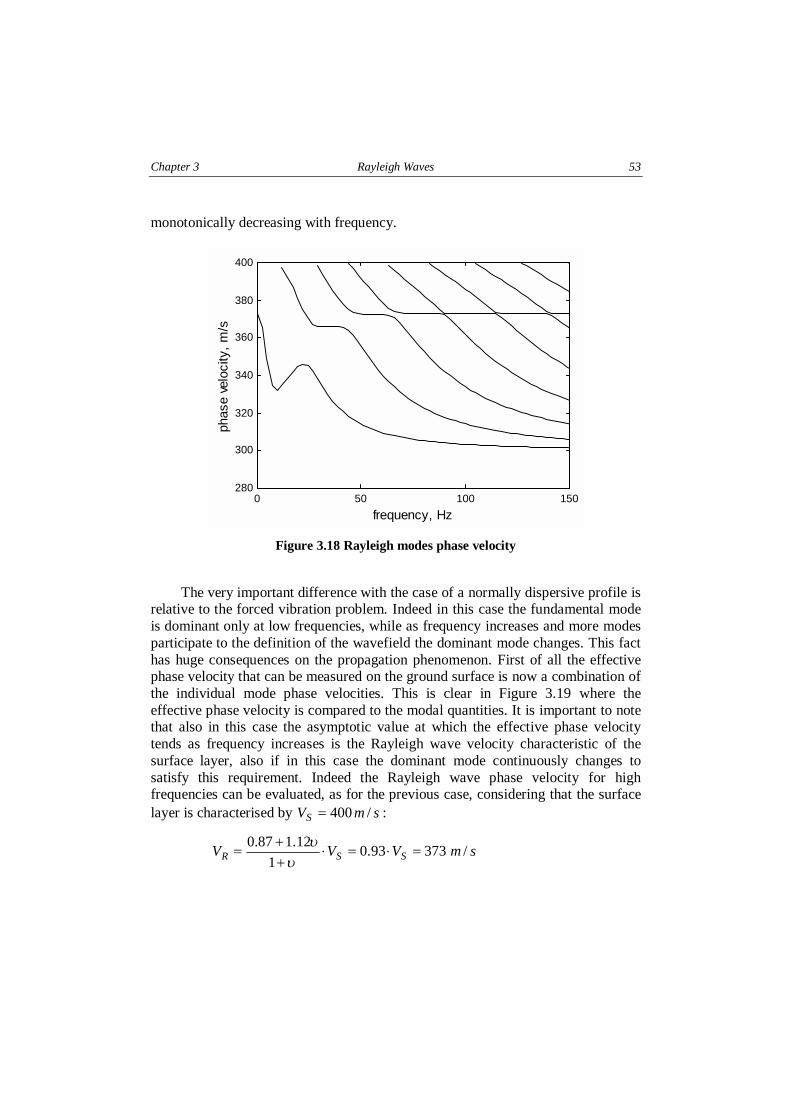
With regards to the solution of the eigenproblem that is associated to the freeRayleigh vibration, the only essential difference with respect to the previousanalysed case of a normally dispersive profile, is given by the shape of the modaldispersion curves (Figure 3.18). Note that in this case, the phase velocity is not


monotonically decreasing with frequency.

0 50 100 150280

300

320

340

360

380

400

frequency, Hz

phas

e ve

loci

ty,

m/s

Figure 3.18 Rayleigh modes phase velocity

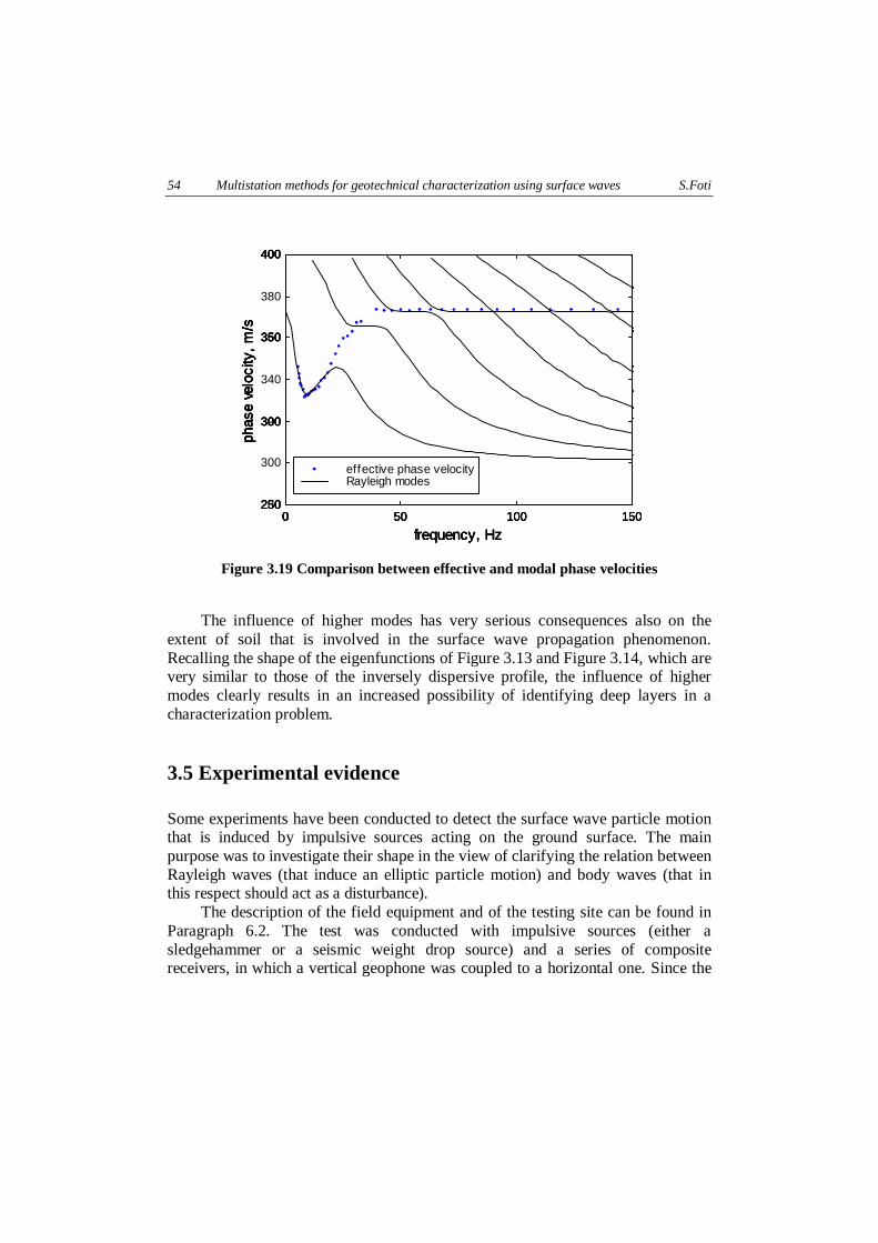
The very important difference with the case of a normally dispersive profile isrelative to the forced vibration problem. Indeed in this case the fundamental modeis dominant only at low frequencies, while as frequency increases and more modesparticipate to the definition of the wavefield the dominant mode changes. This facthas huge consequences on the propagation phenomenon. First of all the effectivephase velocity that can be measured on the ground surface is now a combination ofthe individual mode phase velocities. This is clear in Figure 3.19 where theeffective phase velocity is compared to the modal quantities. It is important to notethat also in this case the asymptotic value at which the effective phase velocitytends as frequency increases is the Rayleigh wave velocity characteristic of thesurface layer, also if in this case the dominant mode continuously changes tosatisfy this requirement. Indeed the Rayleigh wave phase velocity for highfrequencies can be evaluated, as for the previous case, considering that the surfacelayer is characterised by smVS /400' :

smVVV SSR /37393.01

12.187.0 '&'&++

':

:


0 50 100 150250

300

350

400

frequency, Hz

phas

e ve

loci

ty,

m/s


0 50 100 150250

300

350

400

frequency, Hz

phas

e ve

loci

ty,

m/s


0 50 100 150250

300

350

400

frequency, Hz

phas

e ve

loci

ty,

m/s

0 50 100 150250

300

350

400

frequency, Hz

phas

e ve

loci

ty,

m/s


0 50 100 150280

300

320

340

360

380

400

frequency, Hz

phas

e ve

loci

ty,

m/s


Figure 3.19 Comparison between effective and modal phase velocities

The influence of higher modes has very serious consequences also on theextent of soil that is involved in the surface wave propagation phenomenon.Recalling the shape of the eigenfunctions of Figure 3.13 and Figure 3.14, which arevery similar to those of the inversely dispersive profile, the influence of highermodes clearly results in an increased possibility of identifying deep layers in acharacterization problem.

3.5 Experimental evidence

Some experiments have been conducted to detect the surface wave particle motionthat is induced by impulsive sources acting on the ground surface. The mainpurpose was to investigate their shape in the view of clarifying the relation betweenRayleigh waves (that induce an elliptic particle motion) and body waves (that inthis respect should act as a disturbance).

The description of the field equipment and of the testing site can be found inParagraph 6.2. The test was conducted with impulsive sources (either asledgehammer or a seismic weight drop source) and a series of compositereceivers, in which a vertical geophone was coupled to a horizontal one. Since the


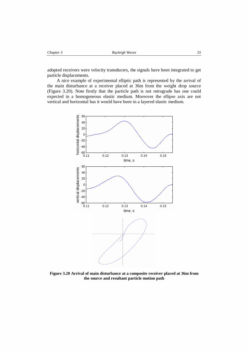
adopted receivers were velocity transducers, the signals have been integrated to getparticle displacements.

A nice example of experimental elliptic path is represented by the arrival ofthe main disturbance at a receiver placed at 36m from the weight drop source(Figure 3.20). Note firstly that the particle path is not retrograde has one couldexpected in a homogeneous elastic medium. Moreover the ellipse axis are notvertical and horizontal has it would have been in a layered elastic medium.

0.11 0.12 0.13 0.14 0.15-60

-40

-20

0

20

40

60

time, s

horiz

onta

l dis

plac

emen

ts

0.11 0.12 0.13 0.14 0.15-60

-40

-20

0

20

40

60

time, s

vert

ical

dis

plac

emen

ts

Figure 3.20 Arrival of main disturbance at a composite receiver placed at 36m fromthe source and resultant particle motion path


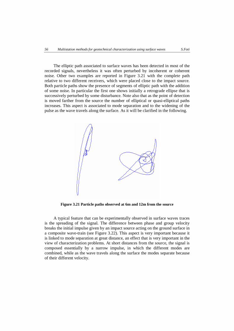
The elliptic path associated to surface waves has been detected in most of therecorded signals, nevertheless it was often perturbed by incoherent or coherentnoise. Other two examples are reported in Figure 3.21 with the complete pathrelative to two different receivers, which were placed close to the impact source.Both particle paths show the presence of segments of elliptic path with the additionof some noise. In particular the first one shows initially a retrograde ellipse that issuccessively perturbed by some disturbance. Note also that as the point of detectionis moved farther from the source the number of elliptical or quasi-elliptical pathsincreases. This aspect is associated to mode separation and to the widening of thepulse as the wave travels along the surface. As it will be clarified in the following.

Figure 3.21 Particle paths observed at 6m and 12m from the source

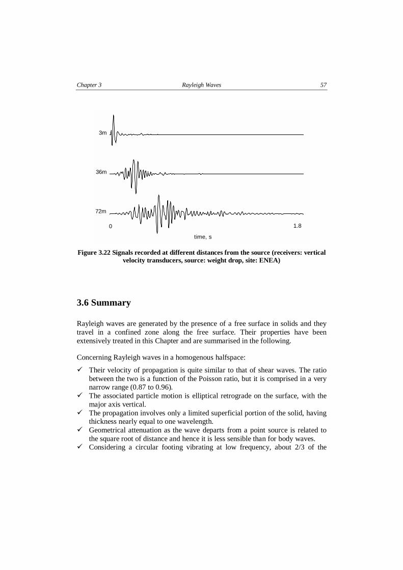
A typical feature that can be experimentally observed in surface waves tracesis the spreading of the signal. The difference between phase and group velocitybreaks the initial impulse given by an impact source acting on the ground surface ina composite wave-train (see Figure 3.22). This aspect is very important because itis linked to mode separation at great distance, an effect that is very important in theview of characterization problems. At short distances from the source, the signal iscomposed essentially by a narrow impulse, in which the different modes arecombined, while as the wave travels along the surface the modes separate becauseof their different velocity.


time, s

0 1.8

3m

36m

72m

Figure 3.22 Signals recorded at different distances from the source (receivers: verticalvelocity transducers, source: weight drop, site: ENEA)

3.6 Summary

Rayleigh waves are generated by the presence of a free surface in solids and theytravel in a confined zone along the free surface. Their properties have beenextensively treated in this Chapter and are summarised in the following.

Concerning Rayleigh waves in a homogenous halfspace:

! Their velocity of propagation is quite similar to that of shear waves. The ratiobetween the two is a function of the Poisson ratio, but it is comprised in a verynarrow range (0.87 to 0.96).

! The associated particle motion is elliptical retrograde on the surface, with themajor axis vertical.

! The propagation involves only a limited superficial portion of the solid, havingthickness nearly equal to one wavelength.

! Geometrical attenuation as the wave departs from a point source is related tothe square root of distance and hence it is less sensible than for body waves.

! Considering a circular footing vibrating at low frequency, about 2/3 of the


input energy goes in surface waves and only the remaining portion in bodywaves.

! Their material attenuation is much more influenced by shear wave attenuationthan by longitudinal waves one.

For a layered system, the following points regarding surface wave propagation areworthily highlighted:

" The phase velocity is frequency dependent also for an elastic medium(geometric dispersion).

" In general for a given frequency several free vibration modes exist, each onecharacterised by a given wavenumber and hence a given phase velocity. Thedifferent modes involve different stress and displacement distributions withdepth.

" It is necessary to distinguish group velocity from phase velocity." Particle motion on the ground surface is not necessarily retrograde." In presence of an external source acting on the ground surface it is necessary to

account for mode superposition that has some major consequences:# The geometrical attenuation is a complicate function of the mechanical

properties of the whole system.# The effective phase velocity is a combination of modal values and it is

spatially dependent.# Because of the difference between phase velocity and group velocity, mode

separation takes place going away from the source and hence the pulsechanges shape.

Finally it is noteworthy to mention the main lessons learned from the numericalsimulations:$ For a normally dispersive profile the fundamental mode is strongly predominant

on the higher modes at every frequency. This has some very importantconsequences:" The effective phase velocity is practically coincident with the fundamental

mode one." The wave propagation interests a portion of the medium nearly equal to a

wavelength$ For an inversely dispersive profile it is very important to account for mode

superposition.

multistation methods for geotechnical characterization...

Documents