multiscale geostatistical analysis of avhrr, spot-vgt, and modis

Multiscale geostatistical analysis of AVHRR, SPOT-VGT,and MODIS global NDVI products

Elena Tarnavsky a,⁎, Sebastien Garrigues b, Molly E. Brown c

a King's College London, Geography Department, United Kingdomb University of Maryland/NASA Goddard Space Flight Center, United States

c Science Systems and Applications, Inc./NASA Goddard Space Flight Center, United States

Received 15 March 2006; received in revised form 15 May 2007; accepted 19 May 2007

Abstract

Global NDVI data are routinely derived from the AVHRR, SPOT-VGT, and MODIS/Terra earth observation records for a range of applicationsfrom terrestrial vegetation monitoring to climate change modeling. This has led to a substantial interest in the harmonization of multisensorrecords. Most evaluations of the internal consistency and continuity of global multisensor NDVI products have focused on time-seriesharmonization in the spectral domain, often neglecting the spatial domain. We fill this void by applying variogram modeling (a) to evaluate thedifferences in spatial variability between 8-km AVHRR, 1-km SPOT-VGT, and 1-km, 500-m, and 250-m MODIS NDVI products over eight EOS(Earth Observing System) validation sites, and (b) to characterize the decay of spatial variability as a function of pixel size (i.e. data regularization)for spatially aggregated Landsat ETM+ NDVI products and a real multisensor dataset. First, we demonstrate that the conjunctive analysis of twovariogram properties – the sill and the mean length scale metric – provides a robust assessment of the differences in spatial variability betweenmultiscale NDVI products that are due to spatial (nominal pixel size, point spread function, and view angle) and non-spatial (sensor calibration,cloud clearing, atmospheric corrections, and length of multi-day compositing period) factors. Next, we show that as the nominal pixel sizeincreases, the decay of spatial information content follows a logarithmic relationship with stronger fit value for the spatially aggregated NDVIproducts (R2=0.9321) than for the native-resolution AVHRR, SPOT-VGT, and MODIS NDVI products (R2=0.5064). This relationship serves as areference for evaluation of the differences in spatial variability and length scales in multiscale datasets at native or aggregated spatial resolutions.The outcomes of this study suggest that multisensor NDVI records cannot be integrated into a long-term data record without proper considerationof all factors affecting their spatial consistency. Hence, we propose an approach for selecting the spatial resolution, at which differences in spatialvariability between NDVI products from multiple sensors are minimized. This approach provides practical guidance for the harmonization oflong-term multisensor datasets.© 2007 Elsevier Inc. All rights reserved.

Keywords: AVHRR; SPOT-VGT; MODIS; Landsat; NDVI; Geostatistics; Variograms; Variogram modeling; Spatial variability; Variogram sill; Length scale; EOSsites; Global vegetation monitoring; Multisensor; Multiscale

1. Introduction

Successful monitoring of terrestrial ecosystems at the regionaland global scales requires frequent and internally consistentrecords providing information on the spatial complexity andtemporal dynamics for a range of biophysical variables. Suchinformation is now regularly produced from remotely sensedimages processed into spectral vegetation indices (Cracknell,

2001; DeFries & Belward, 2000). The normalized differencevegetation index (NDVI) has become one of themost widely usedindices routinely derived from NOAA AVHRR images since1981 (Cracknell, 2001; Tucker, 1979, 1980). Since the 1980s,considerable effort has gone into generating multi-day vegetationindex composites for global vegetation monitoring and climatechangemodeling. The algorithms for generating vegetation indexrecords through compositing of daily measurements reduce noiseand atmospheric effects present in the direct reflectancemeasurements (Holben, 1986; Huete et al., 2002; Myneni et al.,1995; Sellers, 1985).Multi-day vegetation index composites have

Available online at www.sciencedirect.com

Remote Sensing of Environment 112 (2008) 535–549www.elsevier.com/locate/rse

⁎ Corresponding author.E-mail address: [email protected] (E. Tarnavsky).

0034-4257/$ - see front matter © 2007 Elsevier Inc. All rights reserved.doi:10.1016/j.rse.2007.05.008

mailto:[email protected]

http://dx.doi.org/10.1016/j.rse.2007.05.008

been shown to be highly sensitive to biophysical variables such asphotosynthetically active biomass (Goetz et al., 1999), chloro-phyll abundance (Dawson et al., 2003; Gitelson et al., 2002),presence of green vegetation and energy absorption (Myneniet al., 1995; Tucker, 1979).

The sensitivity of NDVI to a broad range of terrestrialecosystem parameters has not only extended the use of multi-dayNDVI composites far beyond intended applications (Cracknell,2001), but has also stimulated the development of new imaginginstruments. As result, NDVI data is now derived from a numberof moderate resolution sensors that have improved upon thespatial, spectral, and radiometric properties of AVHRR (Myneniet al., 1995; Tucker, 1979). The SPOT-Vegetation (SPOT-VGT)and MODIS imaging sensors have accumulated several years ofNDVI data since 1998 and 2000, respectively, and are widelyregarded as improved measurements of surface vegetation con-dition and dynamics (Huete et al., 2002; Justice et al., 2000;Maisongrande et al., 2004). As a result, the user community hasaccess to an extensive global record of multisensor, multi-dayNDVI composites for use in biophysical monitoring and climatechange modeling. Many users, such as the USDA Foreign Agri-culture Service and USAID Famine Early Warning System, havefound that often a combination of all available sources is moreuseful, as each imaging system has different length of record aswell as spatial, temporal, and radiometric characteristics (VanLeeuwen et al., 2006). Although the use of multisensor data canhelp to fill gaps in spatial and temporal coverage, differencesbetween sensor characteristics can hinder the successful integra-tion of multisensor datasets.

The increasing availability and accessibility of multisensorglobal NDVI products and the growing interest in their inte-gration into dynamic models, prompts the need to investigatetheir spatial and temporal consistency in order to facilitate (a) thedevelopment of a continuous and internally consistent NDVItime-series record, and (b) the harmonization of multisensorrecords for simultaneous or interchangeable use (Van Leeuwenet al., 2006). Substantial part of research in this direction hastargeted quantifying the spectral differences between NDVIproducts mostly in the temporal domain (Brown et al., 2006;Goetz, 1997; Justice et al., 2000; Steven et al., 2003; Thomlinsonet al., 1999; Tucker et al., 2005). However, relatively little re-search has focused on assessing the spatial consistency of multi-sensor records. To address this need, we quantify and evaluatethe differences in spatial variability for a multisensor, multi-resolution NDVI dataset selected from the widely used AVHRR,SPOT-VGT, and MODIS NDVI records.

In remote sensing images, spatial variability is mainly relatedto the scale (defined in terms of spatial extent and spatial reso-lution), at which the data are collected and analyzed, and referredto as length scale (Blöschl & Silvapalan, 1995). There are threeinter-related spatial scaling components in imaging, namelyground sampling distance (GSD), point spread function (PSF),and spatial extent of images. GSD describes the intrinsicresolution of images as a function of the sensor's view angle withincreasing GSDwith off-nadir view angles. The value of GSD atnadir determines the nominal pixel size of sensors. Sensorsystems apply to the radiometric signal a low-pass spatial filter,

known as the PSF. The PSF describes the distribution of therelative intensity of a point light source as a function of distancefrom the center of the light source, and characterizes the resultantmulti-directional blurring. The size of the actual spatial supportof the data (the area over which radiometric signal is integrated)is a function of both GSD and PSF and is generally larger thanthe nominal pixel size as determined by the GSD. While GSDdetermines the highest, the spatial extent of images determinesthe smallest spatial frequencies represented in the data. Inaddition to these spatial components, spatial variability ofremote sensing products is also affected by non-spatialcomponents of the image processing chain such as griddingmechanisms, atmospheric correction, cloud screening, calibra-tion, and length of the multi-day compositing period, the latterrecently individually evaluated in Fensholt et al. (2007).

Here, our objective is to quantify and evaluate the spatialvariability and length scales for a multisensor NDVI datasetthrough two geostatistical components, namely the overall imagespatial variance (sill) and the characteristic length scale (meanlength scale metric) (Blöschl & Silvapalan, 1995; Garrigues et al.,2006). The mean length scale represents the characteristic spatialscale of image features such as forest patches and agriculturalfields. These two components can be quantified using variogrammodeling (Curran, 1988, 2001; Garrigues et al., 2006; Milne &Cohen, 1999; Woodcock et al., 1988a,b). The variogram is apowerful geostatistical tool for understanding the loss of spatialinformation content as spatial resolution decreases (Curran &Atkinson, 1999; Jupp et al., 1988, 1989;Woodcock et al., 1988a,b),and thus, it is applied to the multi-resolution NDVI dataset here.

Although several studies have investigated spatial variabilityin relation to spatial resolution through variogram analysis, thesehave been mostly applied to single-sensor images that have beenspatially aggregated to multiple resolutions (Chen, 1999;Garrigues et al., 2006; Woodcock et al., 1988a,b). Goodin andHenebry (2002) took this approach further and quantified thedecay of spatial variability for realmulti-resolution data; however,their analyses included high spatial resolution aerial photographsand covered a small range of spatial resolutions from 0.625 to3.125 m pixel size. Using simulated data, Tan et al. (2006)assessed the differences of spatial information content of MODISproducts by examining the individual effects of spatial resolution,point spread function (PSF), gridding (assigning sensor observa-tions to grid cells), aggregation, and compositing methods. Al-though the Tan et al. (2006) study helped to better understand thefactors affecting spatial variability in remote sensing images, itonly considered data from the MODIS sensor, for which detailedsensor characterization is available. Finally, most studies werelimited to analysis of experimental variograms, while consider-ably less attention was given to variogram modeling for explicitquantitative analysis of both components of spatial variability,namely the overall image variance and the mean length scale.

In order to evaluate the impact of spatial resolution on thespatial variability captured by the widely used NDVI datasets,we characterize the differences in spatial variability between 8-km AVHRR, 1-km SPOT-VGT, and 1-km, 500-m, and 250-mMODIS NDVI products through geostatistical modeling. Theoutcomes of this study help users to understand the differences in

536 E. Tarnavsky et al. / Remote Sensing of Environment 112 (2008) 535–549

spatial information content in relation to the key spatial compo-nents described above. Further, we propose a practical approachfor determining the spatial resolution, at which differences be-tween datasets in the spatial domain are minimized.

2. Data

2.1. Characteristics of EOS sites and selection of NDVI subsets

For evaluation of spatial variability in AVHRR, SPOT-VGT,and MODIS NDVI products, we utilized image subsets for eightEarth Observing System (EOS) land validation core sites(NASA-GSFC, 2006) as illustrated in Fig. 1. The EOS sites areintended for validation of satellite-based land imaging sensorsover a range of biome types. The eight EOS sites consideredhere represent the broadleaf forest (Harvard and Ji-Parana),shrubland/woodland (Jornada and Mongu), broadleaf cropland(Bondville), and grassland/cereal crop (Konza Prairie, Mandal-gobi, and Uardry) biomes.

The AVHRR, SPOT-VGT, and MODIS NDVI subsets wereselected from nearly the same multi-day compositing period (lateAugust to early September 2001) and cropped to cover spatiallyidentical area of approximately 44,000 km2 (220 by 220 km) asshown in Fig. 2 for the Harvard site. The image subsets corres-pond to the relatively homogeneous EOS field sites, covering anarea of approximately 31,400 km2 within the 44,000 km2 extent

of image subsets (Morisette et al., 2002). The identical spatialextent forNDVI subsets frommultiple sources ensures that spatialvariability is compared over the same imaged land surface. Cloudand water pixels, as well as missing NDVI values, were excludedfrom the computation of spatial variability.

2.2. Description of NDVI data sources

An overview of sensor specifications and NDVI datasets isprovided in Table 1 with further discussion of the differencesbetween the spectral properties such as waveband width inTrishchenko et al. (2002) and Van Leeuwen et al. (2006).

2.2.1. AVHRR 8-km NDVI compositesThe AVHRRNDVI subsets for the eight EOS sites included in

this study were obtained from the NASA Global InventoryMapping and Monitoring System (GIMMS) group through theMODIS Land Validation Team web site (NASA-GSFC, 2006).The GIMMS group has generated 15-day maximum valueAVHRR NDVI composites at 8 km spatial resolution. Real-timeAVHRR data is sampled on board the satellite to produce a GlobalArea Coverage (GAC) dataset at reduced spatial resolution byaveraging four out of every five samples along the scan line, andprocessing data from only every third scan line. Scan dimensionsof GAC data at nadir are 1.1 km by 4.4 km with a 3.3-km gapbetween pixels across the scan line. As result, the spatial

Fig. 1. Location and characteristics of the eight Earth Observing System (EOS) land validation sites used for evaluation of multisensor NDVI products.

537E. Tarnavsky et al. / Remote Sensing of Environment 112 (2008) 535–549

resolution at nadir is 4.36 km (crosstrack average) by 1.09 km(along track) at 833 km altitude, but is generally treated as 4 kmresolution (NOAA, 2000; Townshend, 1994). Subsequently, eachGAC pixel is binned into one of the projected 8-km pixels of theoutput product. Therefore, data recorded with different viewangles may contain distortion and bi-directional reflectanceeffects (James & Kalluri, 1994). The GIMMS NDVI datasetshave been corrected for sensor degradation and intercalibrationdifferences, global cloud cover contamination, viewing angleeffects due to satellite drift, volcanic aerosols, and low signal-to-noise ratios due to sub-pixel cloud contamination and watervapor. Although relatively coarse resolution, the resulting globaldataset, known as the GIMMS NDVIg, is the only publiclyavailable AVHRR dataset to extend from 1981 to present and isthus widely used for near real-time global vegetation monitoring(Brown et al., 2004; Pinzon et al., 2005; Tucker et al., 2005).

2.2.2. SPOT-VGT 1-km NDVI compositesThe SPOT-VGT NDVI subsets obtained from the MODIS

Land Validation Team web site (NASA-GSFC, 2006) are 10-daycomposites at 1-km spatial resolution. The SPOT-VGT sensor isequippedwith awide-angle CCD chip cameras, avoidingmuch of

the spatial distortion at off-nadir viewing angles observedwith theAVHRR scanning instrument. Additionally, data from the SPOT4 platform outperforms the AVHRR sensor data in terms ofnavigation, radiometric sensitivity, and four spectral bands insteadof two in the visible-to-infrared part of the electromagneticspectrum (Gobron et al., 2000). The SPOT-VGT S10 (10-day)NDVI composites at full resolution of 1 kmare generated from theatmospherically corrected P products (surface reflectance cor-rected for molecular and aerosol scattering, water vapor, ozoneand other gas absorption) through maximum value compositing(Holben, 1986). The P products are corrected for band-to-bandmisregistration effects and linearity of radiometric response(CNES, 2006). The SPOT-VGT cloud clearing, atmosphericcorrection, and bi-directional compositing procedures substan-tially reduce the noise in reflectance andNDVI that is due to cloudand aerosol presence and the viewing geometry of the sensorsystem at the time of imaging (Maisongrande et al., 2004).

2.2.3. MODIS 1-km, 500-m, and 250-m NDVI compositesFor this study, Version 4MODIS/Terra NDVI products (1-km

MOD13A2, 500-m MOD13A1, and 250-m MOD13Q1) wereobtained from the EOS Data Gateway (NASA-EOS, 2006). The

Table 1Characteristics of the AVHRR, SPOT-VGT, and MODIS imaging systems and the respective NDVI datasets

System characteristics NOAA AVHRR SPOT-VGT MODIS Terra

NDVI data source AVHRR GIMMS SPOT-VGT S10 MOD13A2 MOD13A1 MOD13Q1Spatial characteristicsa. Nominal pixel size 8 km 1 km 1 km 500 m 250 mb. Subset size (pixels) 25!25 201!201 218!218 434!434 866!866

Radiometric quantization 10-bit 8-bit 12-bit 12-bit 12-bitSpectral wavelength/bandwidth (nm)a. Red 580–680/100 610–680/70 620–670/50 620–670/50 620–670/50b. NIR 730–980/250 780–890/110 840–880/40 840–880/40 840–880/40

Multi-day compositing 15-day 10-day 16-day 16-day 16-daya. Period (mm/dd-mm/dd, 2001) 09/01–09/15 09/01–09/10 a 08/29–09/13 08/29–09/13 08/29–09/13b. Method MVC MVC CV–MVC CV–MVC CV–MVC

Off-nadir view angle (degrees) 55.4 50.5 65 65 65

MVC=maximum value composite; CV–MVC=constrained maximum value composite.a SPOT-VGT 09/10–09/20 was used for Mandalgobi and Mongu EOS sites due to cloud cover in the 09/01–09/10 data.

Fig. 2. AVHRR, SPOT-VGT, and MODIS normalized difference vegetation index (NDVI) subsets at full spatial extent (approximately 220!220 km) for the HarvardEOS (Earth Observation System) validation site.


MODIS vegetation index 16-day composite products (MOD13series) were designed to continue the 20+ years NOAAAVHRR-derived NDVI time series (Huete et al., 2002). As a Level 3product, these are computed from the Level 2 daily surfacereflectance product (MOD09 series) corrected for molecular andaerosol scattering, and ozone absorption (Vermote et al., 2002).The 1-km MOD13 products are generated through aggregationof the red (band 1) and near-infrared (band 2) from their native250-m resolution via the MODIS Gridding and AggregationProcess. The gridding and aggregation algorithms, along with aproposed weighting algorithm to account for the triangular PSF(along-scan direction) and approximately rectangular PSF(along-track direction) of the MODIS instrument are describedin detail in Wolfe et al. (1998), Huete et al. (2002), and Tan et al.(2006). Unlike AVHRR and SPOT-VGT, the MODIS NDVIcomposites are generated through a constrained view maximumvalue compositing (CV-MVC) method. This approach isdesigned to address the angular variations that are inherent tomost space-based imaging instruments and reduces the spatialand temporal discontinuities in the multi-day composites (Hueteet al., 2002).

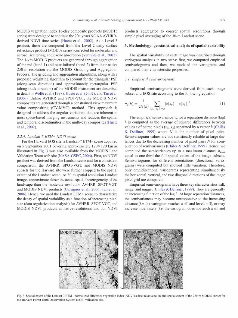
2.2.4. Landsat-7 ETM+ NDVI sceneFor the Harvard EOS site, a Landsat-7 ETM+ scene acquired

on 5 September 2001 covering approximately 120!120 km asillustrated in Fig. 3 was also available from the MODIS LandValidation Team web site (NASA-GSFC, 2006). First, an NDVIproduct was derived from the Landsat scene and for a consistentcomparison, the AVHRR, SPOT-VGT, and MODIS NDVIsubsets for the Harvard site were further cropped to the spatialextent of the Landsat scene. At 30 m spatial resolution Landsatimages approximate closer the actual spatial heterogeneity of thelandscape than the moderate resolution AVHRR, SPOT-VGT,and MODIS NDVI products (Garrigues et al., 2006; Tan et al.,2006). Hence, we used the Landsat ETM+ scene to characterizethe decay of spatial variability as a function of increasing pixelsize (data regularization analysis) for AVHRR, SPOT-VGT, andMODIS NDVI products at native-resolutions and for NDVI

products aggregated to coarser spatial resolutions throughsimple pixel averaging of the 30-m Landsat scene.

3. Methodology: geostatistical analysis of spatial variability

The spatial variability of each image was described throughvariogram analysis in two steps: first, we computed empiricalsemivariograms and then, we modeled the variograms andcompared their characteristic properties.

3.1. Empirical semivariograms

Empirical semivariograms were derived from each imagesubset and EOS site according to the following equation:

ge!h" #1

2N!h"X

txa$xbtch

!z!xa" $ z!xb""2: !1"

The empirical semivariance !e for a separation distance (lag)h is computed as the average of squared differences betweenvalues z of paired pixels (x", x#) separated by a vector h (Chilès& Delfiner, 1999) where N is the number of pixel pairs.Semivariogram values are not statistically reliable at large dis-tances due to the decreasing number of pixel pairs N for com-putation of semivariances (Chilès & Delfiner, 1999). Hence, wecomputed the semivariances up to a maximum distance hmax

equal to one-third the full spatial extent of the image subsets.Semivariograms for different orientations (directional vario-grams) were computed but showed little variation. Therefore,only omnidirectional variograms representing simultaneouslythe horizontal, vertical, and two diagonal directions of the imagepixel grid are compared.

Empirical semivariograms have three key characteristics: sill,range, and nugget (Chilès & Delfiner, 1999). They are generallyan increasing function of the lag h. At large separation distances,the semivariances may become unresponsive to the increasingdistance (i.e. the variogram reaches a sill and levels-off), or mayincrease indefinitely (i.e. the variogram does not reach a sill and

Fig. 3. Spatial extent of the Landsat-7 ETM+ normalized difference vegetation index (NDVI) subset relative to the full spatial extent of the 250-m MODIS subset forthe Harvard Forest Earth Observation System (EOS) validation site.


is unbound). The sill is an indicator of the overall spatial varianceof the data. If the sill is not reached before hmax, the spatial extentof the image is not sufficiently large to encompass the lowfrequency variation in the data (Chilès & Delfiner, 1999). This isgenerally due to spatial structures that extend beyond the spatialextent of the image subsets creating apparent trends in the image.The variograms under study here generally show more than onerange (Fig. 4), indicating spatial structuring of the data atmultiple scales. The largest range is the distance at which thevariogram reaches the sill and values of pixel pairs separated bydistances larger than the largest range are spatially uncorrelated(Chilès & Delfiner, 1999). The behavior of the variogram nearthe origin is also an important property characterizing the spatialcontinuity and the regularity of the data. A discontinuity of thevariogram near the origin (nugget effect) is related to eitheruncorrelated noise (measurement error) or to spatial structuresthat are prominent at spatial scales smaller than the pixel size.The nugget effect however is more common with high spatialresolution imagery (Atkinson, 1999; Curran, 1988) and accordingto change of support theory (Chilès&Delfiner, 1999), it decreasesconsiderably as pixel size increases. In addition, the blurringeffect induced by PSF associated with each sensor further reducesthe nugget effect. Hence, we assume that for the relatively coarseresolution datasets considered here, the nugget effect issufficiently small and can be neglected. This decision is con-firmed through the variogram modeling (Section 3.2).

3.2. Variogram modeling

Theoretical variogram models are typically fit throughempirical semivariograms to quantify the spatial variability com-ponents, namely overall image variance and length scales (Chilès& Delfiner, 1999; Webster & Oliver, 2001). Variogram modelingis based on a probabilistic approach considering the image as oneamong all possible realizations of a second-order stationaryrandom function Z(x) (Chilès & Delfiner, 1999). The theoreticalvariogram model of Z(x) in the following expression:

g!h" # 12Var%Z!x& h" $ Z!x"'; !2"

is estimated by fitting a valid mathematical function to eachempirical semivariogram (Chilès &Delfiner, 1999). To account forthe multiscale spatial structuring of the data (Fig. 4), we used alinear model of regionalization (Chilès & Delfiner, 1999) definedas a linear combination of two or more functions as follows:

g!h" # r2Xk#l

k#1

bkgk!rk ; h" !3"

In Eq. (3), !(h) is the modeled variogram, $2 is the variogram sill(i.e. overall image variance), bk is the fraction of overall imagevariance $2 related to each range rk, gk denotes each elementaryvariogram function, and rk is the variogram range related to eachfunctiongk. To confirm the decision to neglect the nugget effect, wefirst modeled experimental variograms with a nugget component(results not reported) and found that the fraction of overall variancebk associated with the nugget effect is sufficiently small, i.e. always

b10% and in most cases b5%. Hence, we focused the analysis onthe sill and range variogram properties.

A linear combination of one exponential and one sphericalelementary variogram functions gk was found to mostaccurately fit the experimental variograms. While for thespherical model (Eq. (4)) the range r2 is the distance, at whichthe sill is actually reached, for the exponential model (Eq. (5))the practical range r1 is the distance, at which the variogramreaches 95% of the sill.

g1!h" # r2 1$ exp $ 3hr

! "! "!4"

g2!h" #r2

32hr$ 12

hr

! "3 !

if h V r

r2if h N r

8>>><

>>>:!5"

The parameters of !(h) are automatically estimated by aniterative weighted least square optimization (Cressie, 1985)where the ranges r1 and r2 are investigated between a minimumdistance (dmin) and maximum distance (dmax) with a discretiza-tion step equal to the spatial resolution of each dataset. For eachpair of range values (r1, r2) being evaluated, the overall variance$2 and the weights b1 and b2 of the exponential and the sphericalmodels, respectively, are estimated using a non-linear leastsquares approach. The mean square difference between the esti-mated and the experimental variograms defined as:

Cr # 1Nd

XNd

i#1

!g!hi" $ ge!h""2 !6"

is evaluated over the Nd class of distances used to compute theexperimental variogram. The parameters $2, b1 and b2, and r1 andr2, which minimize the criteria Cr are reported as model solutions.

As suggested in Chilès and Delfiner (1999), dmin is optimallyselected to be equal to the pixel size of the image, while dmax is setto one-half of the spatial extent of the image subset. Selecting dmax(110 km) larger than the limit distance hmax (73 km) used tocompute the experimental variograms indicates whether the sill isreached at a range smaller or larger than hmax. Since experimentalvariograms are not statistically reliable for distances larger thanhmax, any estimated variogram ranges r2 above dmax are deemed notreliable, and are therefore not considered in the comparison ofvariogram parameters. In these cases, the underlying second-orderstationarity hypothesis, on which variogram modeling relies, isrejected.

Additionally, the integral range A (Chilès & Delfiner, 1999),which summarizes all structural parameters of the variogrammodel (rk and bk) into a single characteristic area-based metric A(the integral range), is also computed according to the followingequation:

A # 1r2

Z

haR2!r2 $ g!h""dh: !7"

The integral range of the linear model of regionalizationis computed as A #

Plk#1 bkAk ; where A1 #

2kr219

for the


exponential and A2 #kr225for the spherical functions. Garrigues et al.

(2006) used the square root of the integral range A, denoted asDc,to quantify the mean length scale of spatially aggregated images.Since Dc is the weighted average of the range parameters, it is

particularly appropriate to compare length scales of multiscaledatasets and is thus adopted here.

Through the variogram sill $2 and the mean length scalemetricDc, we evaluated spatial variability in relation to pixel size,

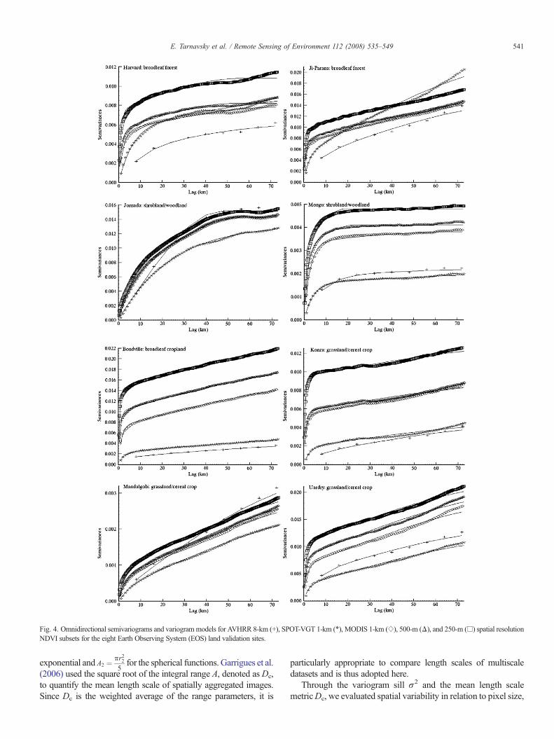
Fig. 4. Omnidirectional semivariograms and variogram models for AVHRR 8-km (+), SPOT-VGT 1-km (⁎), MODIS 1-km (⋄), 500-m (Δ), and 250-m (!) spatial resolutionNDVI subsets for the eight Earth Observing System (EOS) land validation sites.


a concept referred to as data regularization (Jupp et al., 1988,1989). This analysis was applied to characterize the decay ofspatial variability for NDVI products generated through spatialaggregation of the 30-m Landsat-7 ETM+ scene, and provided areference for the loss of spatial variability with increasing pixelsizes of the AVHRR, SPOT-VGT, and MODIS data for the EOSsites, for which the r2b73 km criteria (Section 3.2) was met.According to change of support geostatistical theory (Chilès &Delfiner, 1999), increasing size of the spatial support of data leadsto (a) decrease of the variogram sill, (b) detection of large-scalevariations only, and (c) respective loss of short-scale variationssmaller than two times the pixel size as stated in the Nyquist–Shannon sampling theorem (Nyquist, 1928; Shannon, 1949); thelatter is reflected in increasing Dc values.

4. Results and discussion

First, we evaluate the differences in spatial variability betweenmultisensor NDVI products over the eight EOS sites consideredhere through comparison of empirical semivariograms andanalysis of variogrammodel parameters characterizing the overallimage variance (through the variogram sill) and the actual spatialsupport of data (through the mean length scale metric). Next, wecharacterize the decay of spatial information content as pixel sizeincreases (data regularization) over the Harvard EOS site for thespatially aggregated Landsat-7 ETM+ scene and the AVHRR,SPOT-VGT, and MODIS NDVI products at their native spatialresolutions. Finally, we propose an approach for determining thespatial resolution, at which differences between the spatialproperties of multisensor datasets are minimized.

4.1. Spatial variability of multisensor NDVI products

Empirical semivariograms were computed for each site andeach NDVI product up to a distance of 73 km (hmax=220 km/3)and then modeled using the linear model of regionalization(Section 3.2). Empirical semivariograms and variogram modelsare provided in Fig. 4 (Section 3.1), and the respectiveparameters are reported in Table 2.

As illustrated in Fig. 4, the automatic adjustment of modelvariograms performs well for all empirical semivariograms. Formost sites, however, the spherical model range r2 (Table 2,Column 5) of the AVHRR NDVI scene is larger than hmax andmust be interpreted with caution. This is due to the small spatialextent of AVHRR subsets relative to their 8-km spatial resolution,and thus fewer pixel pairs for calculation of semivariances at largelag distances.Only theHarvard, Jornada, andMonguMODIS andthe Jornada AVHRR data have an r2≤73 km and according to thecriteria outlined in Section 3.2, we only consider the variogramparameters $2 and Dc for these three EOS sites. The variogramsfor the other EOS sites are clearly unbounded, i.e. not reaching asill within the spatial extent of the images. This indicates that theirspatial extents relative to spatial resolution are not sufficientlylarge to encompass the spatial variability of the landscape and thequantitative comparison of variograms properties can beuncertain. Hence, we first compare the overall differences inempirical variograms (Fig. 4) across sites and sensors, and then

Table 2Variogram model parameters for the eight EOS validation sites

NDVI datasource

Spatialvariability(sill), $2

Exponential Spherical Meanlengthscale,Dc

r1 b1 r2 b2

(km) (%) (km) (%) (km)

Harvard a

AVHRR 8 km 0.0062 32.0 60 104.0 40 56.3SPOT-VGT 1 km 0.0089 19.0 65 110.0 35 53.4MODIS 1 km 0.0078 6.0 69 73.0 31 32.6MODIS 500 m 0.0082 4.0 67 54.0 33 24.8MODIS 250 m 0.0108 2.8 69 56.3 31 25.0

Ji-ParanaAVHRR 8 km 0.0143 16.0 29 104.0 71 70.0SPOT-VGT 1 km 0.0217 7.0 23 110.0 77 76.4MODIS 1 km 0.0153 3.0 47 110.0 53 63.7MODIS 500 m 0.0155 3.0 51 110.0 49 61.2MODIS 250 m 0.0177 2.3 55 109.8 45 58.2

Jornada a


Mongu a


BondvilleAVHRR 8 km 0.0037 8.0 33 104.0 67 67.6SPOT-VGT 1 km 0.005 7.0 44 110.0 56 65.4MODIS 1 km 0.0153 4.0 47 110.0 53 63.7MODIS 500 m 0.0179 2.5 56 98.0 44 51.6MODIS 250 m 0.0221 1.8 64 94.3 36 44.6

KonzaAVHRR 8 km 0.0041 16.0 24 104.0 76 72.3SPOT-VGT 1 km 0.0044 8.0 42 110.0 58 66.5MODIS 1 km 0.0088 3.0 60 110.0 40 55.0MODIS 500 m 0.0088 2.5 65 110.0 35 51.9MODIS 250 m 0.0127 1.8 75 109.8 25 43.9

MandalgobiAVHRR 8 km 0.0034 8.0 7 104.0 93 79.5SPOT-VGT 1 km 0.0024 14.0 14 110.0 86 81.0MODIS 1 km 0.0028 8.0 21 110.0 79 77.7MODIS 500 m 0.0029 7.0 22 110.0 78 77.2MODIS 250 m 0.0031 5.3 26 109.8 74 74.6

UardryAVHRR 8 km 0.0131 16.0 35 104.0 65 66.8SPOT-VGT 1 km 0.0115 6.0 25 110.0 75 75.6MODIS 1 km 0.0182 4.0 35 110.0 65 70.2MODIS 500 m 0.0200 3.0 40 110.0 60 67.3MODIS 250 m 0.0218 2.8 49 109.8 51 62.1

r1, r2 — range of variogram models; b2, b2 — fractions of total variance $2.a EOS sites, for which the criteria r2≤73 km is met (i.e. variogram reaches

a sill).


focus on the quantitative analysis of the differences in overallimage variance $2 and mean length scale Dc for the Harvard,Jornada, and Mongu sites based on the variogram modelparameters.

4.1.1. Comparison of empirical semivariogramsThe empirical omnidirectional variograms (Fig. 4) illustrate

that for most sites and sensors semivariance consistentlydecreases as nominal pixel size increases. For the Harvard andJi-Parana sites SPOT-VGTsemivariances are lower than these ofthe 1-km MODIS data at short distances and higher at longdistances; for all other sites, SPOT-VGT semivariances areconsistently lower than these of the 1-kmMODIS data, althoughtheir nominal pixel size is approximately 1 km. As confirmedthrough the evaluation of variogram model parameters (Section4.1.2, Section 4.1.3), the actual size of the spatial support of theSPOT-VGT data is larger than that of the 1-km MODIS data,which according to change of support theory explains the lowersemivariances of SPOT-VGT relative to these for the 1-kmMODIS data. For the Jornada and Mongu (Fig. 4), and theMandalgobi and Uardry sites (Fig. 4), the AVHRR semivario-gram is inconsistent with respect to change of support theory.Since this sensor has the largest pixel size, the semivariancesshould be lowest. However, for Mongu and Uardry, these arehigher than the SPOT-VGT semivariances, and for Jornada andMandalgobi, these are close to the 250-mMODIS semivariancesat large distances. This illustrates that semivariances alone arelimited for characterizing the impact of data regularization. Aswe demonstrate next, the evaluation of variogram modelparameters provides a more robust characterization of spatialvariability in relation to spatial factors.

4.1.2. Overall image variance: variogram sill $2

Differences in overall image variance between products arefurther compared on the basis of the variogram sill $2.Consistent with change of support theory, $2 decreased as thepixel size increases from 250-m to 1-km MODIS data for allsites, including the Harvard, Jornada, and Mongu sites, forwhich variograms reach a sill value within the limit distance(Table 2, Column 2). Since the 1-km NDVI product is derivedthrough the aggregation and gridding of 250-m pixels in the redand near-infrared spectral bands (Wolfe et al., 1998), the spatialvariability of these MODIS products is directly related to thenominal pixel size.

As observed for the empirical semivariances, the spatialvariability characterized through the sill for SPOT-VGT isgenerally lower than that of the 1-km MODIS data for theMongu and Jornada sites. This confirms that the actual size of thespatial support of the SPOT-VGT data is larger than that of 1-kmMODIS data. Two additional spatial factors increase the actualsize of the spatial support of the data compared to the nominalpixel size, namely the PSF and view angle of the sensor system(Tan et al., 2006). The width of the PSF at its full maximum,termed the full width at half maximum (FWHM), quantifies thespatial blurring of the radiometric signal, resulting in largerspatial support than the nominal pixel size as demonstrated forhigh spatial resolution aerial images in Tarnavsky et al. (2004).

The 1-km MODIS product is generated through direct spatialaggregation of 250-m pixels in the red and near-infrared bandsand the MODIS PSF is triangular in along-scan and approxi-mately rectangular in along-track direction (Tan et al., 2006;Wolfe et al., 1998), while the SPOT-VGT product is character-ized by a non-rectangular PSF, which results in actual spatialsupport larger than 1 km. Since the 1-km MODIS NDVI isderived through aggregation of 250-m pixels, the effect of theview angle on the size of the spatial support can propagatethrough the gridding and aggregation algorithm to mask therelative effects of other factors (Tan et al., 2006). Moreover, theMODIS NDVI products are generated using the constrained-view maximum value compositing (CV–MVC) algorithm,which accounts for the angular variations in the standard MVCmethod by choosing near-nadir pixels for the multi-day NDVIproduct, thus further limiting the effect of view angle on the sizeof the spatial support of the data (Huete et al., 2002).

Other non-spatial factors may also contribute to the overallspatial variability captured by each sensor (MODIS and SPOT-VGT) and lead to different behavior than that explained throughthe analysis of data regularization. For example, the sill of SPOT-VGT is higher than that of MODIS for the Harvard site (Table 2,Column 2). Non-spatial factors such as the 6-days differencebetween the compositing periods of these two products, cloudclearing, and atmospheric corrections, also contribute to theoverall spatial variability. Similar inconsistencies between the sillvalue and the size of the spatial support are observed for theJornada and Mongu between the AVHRR and SPOT-VGT data(Table 2, Column 2). While change of support theory suggeststhat the sill of AVHRR should be lowest, it is largest for Jornadaand is higher than that of SPOT-VGT for the Mongu site.Although the estimation of the sill is uncertain for the 8-kmAVHRR data due to the small number of pixel pairs at largedistances, this behavior is confirmed by the comparison of empi-rical semivariances, and is likely due to non-spatial factors such asless precise cloud contamination and atmospheric correction ofAVHRR data than that of the SPOT-VGT (Maisongrande et al.,2004) and MODIS (Vermote & Vermuelen, 1999).

These results highlight that the overall spatial variabilityquantified by the variogram sill is affected by both non-spatial(mainly atmospheric correction and cloud contamination) andspatial (determining the actual size of the spatial support)factors. Since non-spatial factors can mask the effect of spatialfactors as observed for the 1-km SPOT-VGT and MODISHarvard data, the variogram sill alone does not provide for acomprehensive evaluation of the effects of data regularization inthe presence of non-spatial factors as encountered with realmultisensor NDVI datasets.

4.1.3. Characteristic length scales: mean length scale metric Dc

The cumulative effect of spatial factors (nominal pixel size,PSF, and view angle) on the spatial variability captured by eachsensor is evaluated through theDc metric (computed as the squareroot of the integral range A) as it less affected by non-spatialfactors than the variogram sill. Consistent with change of supporttheory, the mean length scale Dc decreases with the actual size ofthe spatial support for the MODIS and SPOT-VGT data for all


sites (Table 2, Column 7). If the AVHRR data is considered, thesame holds true for the Harvard, Bondville, and Konza sites(Table 2, Column 7). However, inconsistent Dc values obtainedfor the Jornada AVHRR data, namely Dc 8-km AVHRR≅Dc 1-km, 500-m, and 250-m MODIS (Table 2, Column 7), are likelydue to the small number of pixel pairs at large distances. For theHarvard and Mongu sites, NDVI data associated with relativelysmall nominal pixel size (e.g. 250-m MODIS) capture higherspatial frequencies (low Dc) from the surface than images havinglarge nominal pixel size (e.g. 8-km AVHRR).

The rates of Dc increase from 250-m MODIS through to the1-km MODIS and SPOT-VGT data depend on the spatialheterogeneity of each site and are thus different across sites. Thedata for the Harvard and Mongu sites show a considerableincreases in Dc value between the 500-m and 1-km MODISdata, i.e. approximately 24% for Harvard (from Dc=24.8 to32.6) and approximately 50% for Mongu (from Dc=9.8 to19.5) (Table 2, Column 7). This suggests that both sites containfeatures having length scales smaller than 2 km as most of thespatial variability is no longer captured in images having spatialresolution coarser than 1 km. Conversely, for Jornada, Dc

remains almost constant between the 500-m MODIS and 1-kmMODIS data (from Dc=37.8 to 38.5); however, it differsconsiderably between the 1-km MODIS and SPOT-VGT (fromDc=38.5 to 60.3) (Table 2, Column 7). This highlights that theJornada site contains features having large length scales thanthese in the Harvard and Mongu sites.

Similarly to the results from the comparison of empiricalsemivariances (Section 4.1.1) and variogram sill (Section4.1.2), the 1-km SPOT-VGTandMODIS datasets have differentspatial properties, i.e. Dc for the SPOT-VGT data are alwaysgreater than those for the 1-km MODIS data (Table 2, Column7). This is explained by the non-rectangular PSF of the SPOT-VGT instrument, which substantially increases the actual size ofthe SPOT-VGT spatial support, while the aggregation andgridding algorithm for the 1-km MODIS data takes into accountthe triangular PSF of the instrument in the along-scan and nearly

rectangular PSF in the along-track directions, resulting in size ofspatial support closer to the nominal pixels size (Tan et al.,2006). In the case of Harvard site, for which the effect of thenon-rectangular PSF of SPOT-VGT on the sill is offset by non-spatial factors, Dc allows for evaluation of differences betweenthe length scales of 1-km MODIS and SPOT-VGT datasets.

These results demonstrate that the Dc is more robust forassessing length scale differences and the effect of pixel size onspatial variability as characterized by the variogram sill. Hence,the conjunctive analysis of these two variogram parametersholds great potential for evaluation of multisensor data in thespatial domain as undertaken here.

4.2. Data regularization: Landsat-7 ETM+ NDVI product

The effect of increasing pixel size (i.e. data regularization) onvariogram propertieswas characterized through the overall spatialvariability $2 and the mean length scale Dc for the spatiallyaggregated 30-m Landsat-7 ETM+ NDVI images and theAVHRR, SPOT-VGT, and MODIS NDVI images (with spatialextent as in Fig. 3) at their native spatial resolutions. Empiricalsemivariograms were computed for the native and aggregatedspatial resolution datasets with spatial extent as illustrated inFig. 3 up to a distance of 40 km (hmax=120 km/3) and thenmodeled using the linear model of regionalization (Section 3.2).The empirical semivariograms and variogram models areprovided in Fig. 5, and the respective model parameters arereported in Table 3. All variograms for these image subsets reach asill before hmax (40 km), which indicates that the spatial variabilityis completely encompassed within the spatial extent of the image.This allows for a quantitative assessment of the decay of spatialvariability as pixel size increases to quantify the effect of spatialcomponents in isolation of sensor-dependent factors.

According to change of support theory, $2 decreases and Dc

increases as the pixel size increases (Table 3, Columns 2 and 8).Assuming the variogram of the 30-m Landsat image approx-imates the actual spatial variability of the landscape, the rate of

Fig. 5. Empirical omnidirectional semivariograms and variogram models for the spatially aggregated 30-m Landsat-7 ETM+ NDVI product and the 8-km AVHRR, 1-km SPOT-VGT, and 1-km, 500-m, and 250-m MODIS NDVI products for the Harvard EOS validation site according to the spatial extent shown in Fig. 3.


sill decrease relative to the sill of the 30-m image (Table 3,Column 3) characterizes the loss of landscape spatial variabilityas the pixel size increases. The rate of decay of spatial varia-bility is explained by the Nyquist–Shannon sampling theorem,according to which short length scales (i.e. smaller than twotimes the pixel size) are no longer captured within the coarserresolution images (Nyquist, 1928; Shannon, 1949). Forexample, at 250 m spatial resolution, the 40% loss of overallspatial variability is related to length scales smaller than 500 m,which are not captured by the 250 m scene, while length scaleslarger than 500 m are still detected and comprise the remaining60% of spatial variability. For the native-resolution dataset the

rate of decay is more substantial, i.e. only 26% of spatialvariability is captured at 250 m spatial resolution of the MODISdataset (Table 3, Column 3) and most of the landscape spatialvariability is lost at 8 km in both native and aggregatedresolution datasets (Table 3, Column 3).

Fig. 6 illustrates the loss of spatial information for theaggregated and native-resolution datasets. As pixel size in-creases, $2 decreases and Dc increases following a logarithmicrelationship (Fig. 6) with stronger fit for the aggregated data(R2 =0.9321) than for the native-resolution data (R2 =0.5064) asthe former represents the decay of spatial variability in isolationfrom sensor-dependent and image processing chain differences.

Table 3Variogram model parameters for the 8-km AVHRR, 1-km SPOT-VGT, and 1-km, 500-m, and 250-mMODIS NDVI products at their native spatial resolutions and thespatially aggregated 30-m Landsat-7 ETM+ NDVI data for the Harvard EOS validation site with image subsets according to the spatial extent in Fig. 3

NDVI datasource

Spatialvariability(sill), $2

Rate ofdecay ofspatialvariabilitya

(%)

Exponential Spherical Meanlengthscale,Dc

r1 b1 r2 b2

(km) (%) (km) (%) (km)

Native-resolution dataAVHRR 8 km 0.0004 4 8.0 73 16.0 27 8.7SPOT-VGT 1 km 0.0012 12 8.0 76 9.0 24 6.8MODIS 1 km 0.0017 17 3.0 77 9.0 23 4.1MODIS 500 m 0.0016 16 2.0 75 8.5 25 3.7MODIS 250 m 0.0026 26 1.3 78 6.3 22 2.5ETM+ 30 m 0.0100 – 0.4 82 6.6 18 2.2

Aggregated Landsat dataETM+ 8 km 0.0007 7 8.0 44 24.0 56 14.9ETM+ 1 km 0.0028 28 4.0 82 18.0 18 6.7ETM+ 500 m 0.0042 42 2.0 77 12.5 23 5.0ETM+ 250 m 0.0060 60 1.3 79 10.8 21 4.0ETM+ 30 mb 0.0100 – 0.4 82 6.6 18 2.2a Relative to the sill of ETM+ 30 m; b Source for aggregated datasets.r1, r2 — range of variogram models; b1, b2 — fractions of total variance.

Fig. 6. Decay of spatial information content characterized by decreasing variogram sill $2 and increasing mean length scale metric Dc in relation to the nominal pixelsize of the 8-km AVHRR, 1-km SPOT-VGT, and 1-km, 500-m, and 250-mMODIS NDVI products at their native spatial resolutions and the spatially aggregated 30-mLandsat-7 ETM+ NDVI product.


Similar results are reported for spatially aggregated high-resolution data in Goodin and Henebry (2002). The decay ofspatial information content for native-resolution data is lessstrong than that for spatially aggregated data due to sensor-dependent factors. This is due to spatial factors (PSF andview angle) affecting both the $2 and Dc, and non-spatialfactors (atmospheric correction, cloud screening, length ofcompositing period) affecting mostly $2. Similar logarithmicdecay is observed for the three sites reaching variogramsill, namely Harvard (y=−0.0024ln(x)+0.017, R2 =0.3338),Jornada (y=−0.0032ln(x)+0.0265, R2 =0.7684), and Mongu(y=−0.0016ln(x)+0.0082, R2 =0.9272). The differences be-tween fit values for the Harvard, Jornada, and Mongu datasetsare due to differing spatial heterogeneity of the sites in additionto sensor-dependent spatial and non-spatial factors. Thelogarithmic relationships for the native versus aggregated

spatial resolution datasets, and the native-resolution datasetsfor Harvard, Jornada, and Mongu serve as a reference forevaluation of spatial information decay in other datasets.

4.3. Minimizing multisensor differences in the spatial domain:a proposed strategy

We illustrated that important differences in NDVI spatialvariability are observed in multisensor datasets, even if datasetshave similar nominal pixel size such as the 1-km MODIS andSPOT-VGT records. Accounting for differences in spatialinformation content is thus critical for the successful integrationof multisensor datasets into a long-term data record, or thesimultaneous and interchangeable use of multisensor datasets. Apossible strategy is to aggregate the products at the spatialresolution, at which differences in spatial variability between

Fig. 7. Root mean square error (RMSE) (y-axis) between the empirical semivariances of 1-km MODIS and 1-km SPOT-VGT NDVI products aggregated to spatialresolutions of 2, 4, 6, and 8 km (x-axis) for the eight EOS validation sites.


products are reduced. Here, we identify the pixel size, at whichdifferences in spatial variability between the widely used 1-kmMODIS and SPOT-VGT NDVI products are minimal. This isachieved through aggregation of the 1-km MODIS and SPOT-VGT NDVI products to coarser spatial resolutions of 2, 4, 6, and8 km for the eight EOS sites considered here and evaluation of theoptimal pixel size for comparison of these products based on theroot mean square error (RMSEv) between the semivariances of 1-kmMODIS and SPOT-VGT data at each spatial resolution v. Theresults (Fig. 7) highlight that differences in spatial variabilitybetween the 1-km MODIS and SPOT-VGT NDVI productsgenerally decrease as pixel size increases. For all sites, except theHarvard and Ji-Parana, the rate of RMSE decrease stabilizesbeyond 6 km, suggesting that the spatial resolution of 1-kmdatasets needs to be degraded approximately 6 times, if data fromthese sources is to be used simultaneously or interchangeably.

These results are in agreement with the outcomes of similarstudies, which suggest that remote sensing products must becompared at spatial resolutions coarser than their native spatialresolutions in order to reduce the differences that are due tofactors such as co-registration and differences in actual spatialresolution (Chen et al., 2002; Fernandes et al., 2003; Tan et al.,2006; Weiss et al., 2007). Specifically, Weiss et al. (2007)compared 1-km SPOT-VGT and MODIS products and showedthat only a small fraction of the radiometric signal is actuallyreceived from the SPOT-VGT pixel. The authors (Weiss et al.,2007) proposed aggregation of SPOT-VGT products to 10 kmspatial resolution for conjunctive use with 1-km MODIS data.Through a more rigorous analysis of data regularization effectson spatial variability, we provide practical guidance for effectivecomparison of the 1-km MODIS and SPOT-VGT datasets atspatial resolutions v≥6 km, at which the effects of sensor-specific characteristics in the spatial domain are minimized.

5. Summary and conclusions

In this study, we used variogram modeling to evaluate thedifferences in spatial variability and length scales between 8-kmAVHRR, 1-km SPOT-VGT, and 1-km, 500-m, and 250-mMODIS NDVI data over eight EOS land validation core sites.For better understanding of the differences in spatial variabilityand the decay of spatial variability with increasing pixel size, wecompared empirical semivariograms and demonstrated theefficiency of two variogram model parameters, namely the sill$2 quantifying the overall image variability, and the square rootof the integral range A (the Dc metric) measuring the meanlength scale of the data. We interpreted the results in the contextof change of support theory, which states that with increasingsize of the data spatial support (referred as data regularization),the variogram sill $2 decreases and the mean length scale Dc

increases since only length scales larger than twice the pixel sizeare captured by the sensor according to the Nyquist–Shannonsampling theorem (Nyquist, 1928; Shannon, 1949).

First, we compared the empirical semivariograms for actualmultisensor NDVI datasets over the eight EOS sites consideredhere, and focused the evaluation of variogram properties on thethree EOS sites, for which variograms reached a sill value at a

distance smaller than the maximum distance hmax. Differencesin spatial variability are due to sensor-dependent spatial factors(e.g. nominal pixel size, PSF, and view angle), which determinethe actual size of spatial support of the data, and to sensor-dependent non-spatial factors (e.g. atmospheric correction,cloud screening, calibration, length of compositing period).While the latter affect the variogram sill, the spatial factors aremost effectively characterized through the conjunctive analysisof the sill $2 and the mean length scale metric Dc. Except forthe MODIS data, for which the sill consistently decreases whenthe nominal pixel size increases, we demonstrated that the sillalone cannot be used to assess spatial variability that is due tothe spatial factors since the effect of these can be masked by thatof non-spatial factors. Further, we found that the spatialvariability captured by the SPOT-VGT data is generally muchlarger than that of the 1-km MODIS NDVI due to the non-rectangular PSF and larger view angles of SPOT-VGT as bothfactors increase the size of the actual spatial support. Since the1-km MODIS is derived through aggregation of the 250-m redand near-infrared MODIS bands through an aggregation andgridding algorithm, which takes into account the MODIS PSFand view angle, the actual spatial support of MODIS data iscloser to the nominal pixel size for the 1 km dataset.

Next, through simultaneous analysis of the variogram sill $2

and the mean length scale metric Dc, we quantified the effect ofpixel size on data regularization using a Landsat-7 ETM+ NDVIimage aggregated to coarser spatial resolutions and compared tothe AVHRR, SPOT-VGT, and MODIS native-resolutiondatasets. We showed that as the nominal pixel size increases,the decay of spatial information content (i.e. decrease of the silland increase of the mean length scale) follows a logarithmicrelationship with stronger fit for the spatially aggregatedLandsat data than for the AVHRR, SPOT-VGT, and MODISNDVI products at native spatial resolutions. This relationshipprovides a reference for further evaluations of differences inspatial variability and length scales in multiscale datasets atnative or aggregated spatial resolutions.

Several points identified in this study can be improved byfurther investigations. For most sites, the variograms of all pro-ducts do not reach a sill value, suggesting that the spatial extent ofthe image subsets is not sufficiently large relative to the spatialresolution to encompass the spatial variability of the landscapesimaged within the subsets. In addition, due to the small spatialextent of the subsets relative to the coarse spatial resolution of the8-km AVHRR data, the AVHRR variogram models did notprovide reliable parameters for all sites to explain their atypicalbehaviors according to change of support theory. Hence, furtherstudies need to determine the required spatial extent for imagesubsets in order to provide a more detailed comparison of spatialvariability for multisensor datasets.

This study provides a relative quantification of the cumulativeeffect of all spatial and non-spatial factors to the spatial variabilitycaptured by different NDVI products. Further research is requiredto quantify the effect of individual factors testing firstly theindividual effects of view angle, PSF, and length of the com-positing period. These factors can be tested using concurrentnative-resolution products in conjunction with relatively high


spatial resolution data such as Landsat, approximating the actualspatial variability of imaged landscapes. Here, this was notundertaken due to the lack of accurate PSF information for thesensors being investigated and the lack of concurrently acquiredLandsat scenes for all EOS sites considered here. The approachesfor multisensor data comparisons presented here can be extendedto include additional sites with different types of land features,more recently available data sources such as from the MERISsensor, and/or analysis of moderate to coarse resolution multi-sensor datasets at the global scale.

This investigation makes a substantial contribution to therecent concern over inter-comparison of multisensor, moderate tocoarse resolution datasets. Until now, studies havemainly focusedon spectral normalization of time-series records in the temporaldomain, however spatial information is critical for the compilationof spatially and temporally continuous datasets. We illustrated theconsistencies and inconsistencies in spatial variability betweenglobal NDVI products at resolutions ranging from 250 m to 8 km,and showed that multisensor NDVI records cannot be integratedinto a long-term data record without proper consideration of allfactors affecting their spatial consistency. We identified factorssuch as view angle and PSF that need to be characterized so thatdata fromMODIS can be used interchangeablywith that of SPOT-VGT, AVHRR or similar data sources. A possible strategy toaccount for the differences in the spatial properties of multisensordatasets is to aggregate the products at the spatial resolution, atwhich their spatial variability is minimized. For the eight EOSsites considered here, we found that a spatial resolution of 6 km orcoarser sufficiently limits the spatial variability differencesbetween SPOT-VGTand 1-kmMODIS NDVI data. This strategyhas considerable implications for themuch-needed integration andharmonization of multisensor data for a range of bioclimaticmonitoring and modeling applications.

Acknowledgments

This study benefited from theMODIS Land Team data serverand from the NASA's Earth Observing System (EOS) DataGateway for the AVHRR, SPOT-VGT, and MODIS NDVIproducts.We thankMs. Emery Boose and Prof.WilliamMungerfromHarvard University for providingGIS reference data for theHarvard Forest LTER site. We also thank two anonymousreviewers for providing valuable comments, which helped us toimprove this manuscript.

References

Atkinson, P. (1999). Spatial Statistics. In A. Stein, B. Gorte, & F. Van der Meer(Eds.), Spatial statistics for remote sensing (pp. 57−81). Kluwer.

Blöschl, G., & Silvapalan, M. (1995). Scale issues in hydrological modelling: Areview. In J. D. Kalma & M. Sivapalan (Eds.), Scale issues in hydrologicalmodelling (pp. 9−48). Chicester: Wiley.

Brown, M. E., Pinzon, J. E., Morisette, J. T., Didan, K., & Tucker, C. J. (2006).Evaluation of the consistency of long term NDVI time series derived fromAVHRR, SPOT-Vegetation, SeaWIFS, MODIS, and Landsat ETM+. IEEETransactions Geosciences and Remote Sensing, 44(7), 1787−1793.

Brown,M. E., Pinzon, J. E., & Tucker, C. J. (2004). New vegetation index datasetavailable to monitor global change. EOS Transactions, 85(52), 565−569.

Chen, J. M. (1999). Spatial scaling of a remotely sensed surface parameter bycontexture. Remote Sensing of Environment, 69(1), 30−42.

Chen, J. M., Pavlic, G., Brown, L., Cihlar, J., Leblanc, S. G., White, H. P., et al.(2002). Derivation and validation of Canada-wide coarse-resolution leaf areaindex maps using high-resolution satellite imagery and ground measure-ments. Remote Sensing of Environment, 80(1), 165−184.

Chilès, J. -P., & Delfiner, P. (1999). Geostatistics: modeling spatial uncertainty(pp. 695). New York: Wiley Inter-Science.

CNES (2006). SPOT-VGTuser's guide [online].Available from: http://vegetation.cnes.fr/system/content.html#userguide [Accessed 07 November 2006].

Cracknell, A. P. (2001). The exciting and totally unanticipated success of theAVHRR in applications for which it was never intended. Advances inSpatial Research, 28(1), 233−240.

Cressie, N. (1985). Fitting variogram models by weighted least squares.Mathematical Geology, 17, 563−586.

Curran, P. J. (1988). The semivariogram in remote sensing: An introduction.Remote Sensing of Environment, 24, 493−507.

Curran, P. J. (2001). Remote sensing: Using the spatial domain. Environmentaland Ecological Statistics, 8, 331−344.

Curran, P. J., & Atkinson, P. M. (1999). Issues of scale and optimal pixel size. InA. Stein, B. Gorte, & F. van der Meer (Eds.), Spatial statistics for remotesensing (pp. 115−133). Kluwer.

Dawson, T. P., North, P. R. J., Plummer, S. E., & Curran, P. J. (2003). Forestecosystem chlorophyll content: Implications for remotely sensed estimatesof net primary productivity. International Journal of Remote Sensing, 24(3),611−617.

DeFries, R. S., & Belward, A. S. (2000). Global and regional land covercharacterization from satellite data: An introduction to the special issue.International Journal of Remote Sensing, 21(6 and 7), 1083−1092.

Fensholt, R., Anyamba, A., Stisen, S., Sandholt, I., Pak, E., & Small, J. (2007).Comparison of compositing period length for vegetation index data frompolar-orbiting and geostationary satellites for the cloud-prone region of WestAfrica. Photogrammetric Engineering and Remote Sensing, 73(3), 297−309.

Fernandes, R. A., Butson, C., Leblanc, S., & Latifovic, R. (2003). Landsat-5 TMand Landsat-7 ETM+ based accuracy assessment of leaf area index productsfor Canada derived from SPOT4/VGT data. Canadian Journal of RemoteSensing, 29(2), 241−258.

Garrigues, S., Allard, D., Baret, F., & Weiss, M. (2006). Quantifying spatialheterogeneity at the landscape scale using variogram models. RemoteSensing of Environment, 103, 81−96.

Gitelson, A. A., Kaufman, Y. J., Stark, R., & Rundquist, D. (2002). Novelalgorithms for remote estimation of vegetation fraction. Remote Sensing ofEnvironment, 80, 76−87.

Gobron, N., Pinty, B., Verstraete, M.M., &Widlowski, J. L. (2000). Developmentof spectral indices optimized for the vegetation instrument. Proceedings ofvegetation 2000. Belgirate, Italy, 3–6 April 2000 (pp. 275−280).

Goetz, S. J. (1997). Multi-sensor analysis of NDVI, surface temperature, andbiophysical variables at a mixed grassland site. International Journal ofRemote Sensing, 18(1), 71−94.

Goetz, S. J., Prince, S. D., Goward, S. N., Thawley,M.M., Small, J., & Johnson, A.(1999). Mapping net primary production and related biophysical variables withremote sensing: Application to the BOREAS region. Journal of GeophysicalResearch Atmospheres, 104(D22), 27719−27734.

Goodin, D. G., & Henebry, G. M. (2002). The effect of rescaling on fine spatialresolution NDVI data: A test using multi-resolution aircraft sensor data.International Journal of Remote Sensing, 23(18), 3865−3871.

Holben, B. (1986). Characteristics of maximum-value composite images fromtemporal AVHRR data. International Journal of Remote Sensing, 7(11),1417−1434.

Huete, A., Didan, K., Miura, T., & Rodriguez, E. (2002). Overview of theradiometric and biophysical performance of the MODIS vegetation indices.Remote Sensing of Environment, 83(1 and 2), 195−213.

James, M. E., & Kalluri, S. N. V. (1994). The pathfinder AVHRR land data set:An improved coarse resolution data set for terrestrial monitoring. Interna-tional Journal of Remote Sensing, 15(17), 3347−3363.

Jupp, D. L. B., Strahler, A. H., & Woodcock, C. E. (1988). Autocorrelation andregularization in digital images: I. Basic theory. IEEE TransactionsGeosciences and Remote Sensing, 26(4), 463−473.


http://vegetation.cnes.fr/system/content.html#userguide

http://vegetation.cnes.fr/system/content.html#userguide

Jupp, D. L. B., Strahler, A. H., & Woodcock, C. E. (1989). Autocorrelation andregularization in digital images: II. Simple image models. IEEE Transac-tions Geosciences and Remote Sensing, 27(3), 247−258.

Justice, C., Belward, A. S., Morisette, J., Lewis, P., Privette, J., & Baret, F.(2000). Developments in the ‘validation’ of satellite sensor products for thestudy of the land surface. International Journal of Remote Sensing, 21(17),3383−3390.

Maisongrande, P., Duchemin, B., & Dedieu, G. (2004). Vegetation/SPOT: Anoperational mission for the Earth monitoring: Presentation of new standardproducts. International Journal of Remote Sensing, 25(1), 9−14.

Milne, B. T., & Cohen, W. B. (1999). Multiscale assessment of binary andcontinuous landcover variables for MODIS validation, mapping, andmodeling applications. Remote Sensing of Environment, 70, 82−98.

Morisette, J. T., Privette, J. L., & Justice, C. O. (2002). A framework for thevalidation of MODIS landproducts. Rmote Sensing of Environment, 83,77−96.

Myneni, R. B., Hall, F. G., Sellers, P. J., & Marshak, A. L. (1995). Theinterpretation of spectral vegetation indexes. IEEE Transactions Geos-ciences and Remote Sensing, 33(2), 481−486.

NASA-EOS (2006). NASA Earth observing system data gateway [online].Available from: http://delenn.gsfc.nasa.gov/~imswww/pub/imswelcome/[Accessed 07 November 2006].

NASA-GSFC (2006).MODIS land: MODIS land validation [online]. Availablefrom: http://landval.gsfc.nasa.gov [Accessed 07 November 2006].

NOAA (2000). NOAA KLM user's guide [online].Available from: http://www2.ncdc.noaa.gov/docs/klm/ [Accessed 07 November 2006].

Nyquist, H. (1928). Certain topics in telegraph transmission theory.TransactionsAIEE, 47, 617−644 (Reprint as classic paper in: Proc. IEEE, Vol. 90, No. 2,Feb 2002).

Pinzon, J. E., Brown, M. E., & Tucker, C. J. (2005). Satellite time seriescorrection of orbital drift artifacts using empirical mode decomposition. InN. Huang (Ed.), Hilbert-Huang transform: introduction and applications,chapter 10, part II. applications.

Sellers, P. J. (1985). Canopy reflectance, photosynthesis, and transpiration. In-ternational Journal of Remote Sensing, 6(8), 1335−1372.

Shannon, C. E. (1949). Communication in the presence of noise. Proceedings ofthe Institute of Radio Engineers, 37, 10−21 (Reprint as classic paper in:Proc. IEEE, Vol. 86, No. 2, Feb 1998).

Steven, M. D., Malthus, T. J., Baret, F., Xu, H., & Chopping, M. J. (2003).Intercalibration of vegetation indices from different sensor systems. RemoteSensing of Environment, 88(4), 412−422.

Tan, B., Woodcock, C. E., Hu, J., Zhang, P., Ozdogan, M., Huang, D., et al.(2006). The impact of geolocation offsets on the local spatial properties ofMODIS data: Implications for validation, compositing, and band-to-bandregistration. Remote Sensing of Environment, 105, 98−114.

Tarnavsky, E., Stow, D. A., Coulter, L., & Hope, A. (2004). Spatial andradiometric fidelity of airborne multispectral imagery in the context of land-cover change analyses. GIScience and Remote Sensing, 41(1), 62−80.

Thomlinson, J. R., Bolstad, P. V., & Cohen, W. B. (1999). Coordinatingmethodologies for scaling landcover classifications from site-specific toglobal: Steps toward validating global map products. Remote Sensing ofEnvironment, 70(1), 16−28.

Townshend, J. R. G. (1994). Global data sets for land applications from theadvanced very high resolution radiometer: An introduction. InternationalJournal of Remote Sensing, 15(17), 3319−3332.

Trishchenko, A. P., Cihlar, J., & Li, Z. (2002). Effects of spectral responsefunction on surface reflectance and NDVI measured with moderateresolution satellite sensors. Remote Sensing of Environment, 81, 1−18.

Tucker, C. J. (1979). Red and photographic infrared linear combinations inmonitoring vegetation. Remote Sensing of Environment, 8(2), 127−150.

Tucker, C. J. (1980). Remote sensing of leaf water content in the near infrared.Remote Sensing of Environment, 10(1), 23−32.

Tucker, C. J., Pinzon, J. E., Brown,M. E., Slayback, D., Pak, E.W.,Mahoney, R.,et al. (2005). An extended AVHRR 8-km NDVI data set compatible withMODIS and SPOT-vegetation NDVI data. International Journal of RemoteSensing, 26(20), 4485−4498.

Van Leeuwen, W. J. D., Orr, B. J., Marsh, S. E., & Herrmann, S. M. (2006).Multi-sensor NDVI data continuity: Uncertainties and implications forvegetation monitoring applications. Remote Sensing of Environment, 100,67−81.

Vermote, E., El Saleous, N., & Justice, C. (2002). Atmospheric correction of theMODIS data in the visible and middle infrared: First results. Remote Sensingof Environment, 83(1 and 2), 97−111.

Vermote, E. F., & Vermuelen, A. (1999). Atmospheric correction algorithm:Spectral reflectances (MOD09). NASA contract NAS5-96062 (pp. 107).University of Maryland, Department of Geography.

Webster, R., & Oliver, M. A. (2001). Characterizing spatial processes: thecovariance and variogram (pp. 271). Chichester, UK: John Wiley.

Weiss, M., Baret, F., Garrigues, S., and Lacaze, R. (in Press). LAI and fAPARCYCLOPES global products derived from VEGETATION. Part 2:Validation and intercomparison with MODIS Collection 4 products. Re-mote Sensing of Environment, doi: 10.1016/j.rse.2007.03.001

Wolfe, R. E., Roy, D. P., & Vermote, E. F. (1998). MODIS land data storage,gridding, and compositing methodology: Level 2 grid. IEEE TransactionsGeosciences and Remote Sensing, 36(4), 1324−1338.

Woodcock, C. E., Strahler, A. H., & Jupp, D. L. B. (1988). The use ofvariograms in remote sensing: I. Scene models and simulated images. Re-mote Sensing of Environment, 25(3), 323−348.

Woodcock, C. E., Strahler, A. H., & Jupp, D. L. B. (1988). The use ofvariograms in remote sensing: II. Real digital images. Remote Sensing ofEnvironment, 25(3), 349−379.


http://delenn.gsfc.nasa.gov/~imswww/pub/imswelcome/

http://landval.gsfc.nasa.gov

http://www2.ncdc.noaa.gov/docs/klm/

http://www2.ncdc.noaa.gov/docs/klm/

http://dx.doi.org/doi:10.1016/j.rse.2007.03.001

multiscale geostatistical analysis of avhrr, spot-vgt, and modis

Documents