multiple-year optimization of conservation effort and monitoring effort for a fluctuating population

Journal of Theoretical Biology 230 (2004) 157–171

ARTICLE IN PRESS

*Correspond

E-mail addr

0022-5193/$ - se

doi:10.1016/j.jtb

Multiple-year optimization of conservation effort and monitoringeffort for a fluctuating population

Hiroyuki Yokomizoa,*, Patsy Haccoub, Yoh Iwasaa

aDepartment of Biology, Faculty of Sciences, Kyushu University, Fukuoka 812-8581, Japanb Institute of Biology, Leiden University, P.O. Box 9516, 2300 RA Leiden, The Netherlands

Received 5 January 2004; received in revised form 8 April 2004; accepted 26 April 2004

Available online 19 June 2004

Abstract

We consider optimal conservation strategies for an endangered population. We assume that juvenile survival is affected by

unpredictable environmental fluctuation and can be improved by costly conservation effort. The initial population size is not

accurately known at the time that the conservation effort level is chosen, but the uncertainty of its estimate can be reduced by a

costly monitoring effort. In a previous paper, we analysed the optimal management strategy that minimizes a weighted sum of

extinction probability and economic costs when only a single year is considered. Here we examine the case in which the conservation

period lasts for several years by dynamic programming with incompletely observed process states. We study the optimal levels of the

conservation and the monitoring efforts, and their dependence on the length of the conservation period and other parameters. The

main conclusions are: (1) The optimal conservation effort in the first year depends on the accuracy of the information on the

population size in the first year, but is almost independent of the accuracy of the information in later years. (2) When the risk of

population extinction is small, the optimal conservation effort increases with the uncertainty of the population size. In contrast when

the population is endangered, the optimal conservation effort decreases with the uncertainty of the population size. (3) The optimal

conservation and monitoring efforts both increase with the length of the conservation period, provided that the population is

relatively safe. However, if the population is endangered, both types of effort become smaller when the conservation period

increases.

r 2004 Elsevier Ltd. All rights reserved.

Keywords: Conservation effort; Monitoring effort; Fluctuating population; Multiple-year optimization

1. Introduction

Conservation and management of wild populations often include decision making under considerable uncertainty.Several theoretical studies have been performed on how to deal with such incomplete information (Ludwig, 1996; Engenet al., 1997; Matsuda et al., 1999; Taylor et al., 2000; Milner-Gulland and Akcakaya, 2001). In the case of conservation ofendangered species the management strategy is aimed at saving populations from extinction. The population sizefluctuates due to environmental and demographic stochasticity. Apart from this stochasticity, we need to consider theuncertainty concerning the population size, demographic properties and the effect of conservation effort.

In a previous paper (Yokomizo et al., 2003a), we examined the optimal conservation strategy to improve the survivalof a population under the assumption that the population size is accurately known. We proposed a simple and generalframework to examine how the optimal conservation effort is affected by environmental fluctuation. The survival ofthe population fluctuates due to environmental noise, expressed as a stochastic variable, and it can be improved byconservation effort, which is accompanied by a cost. The total cost was defined as the sum of the extinction probabilitymultiplied by the value of the population and the economic cost of the conservation effort. We analysed the optimalconservation effort for multiple-year optimization by means of dynamic programming. Dynamic programming has

ing author. Fax: +81-92-642-2645.

ess: [email protected] (H. Yokomizo).

e front matter r 2004 Elsevier Ltd. All rights reserved.

i.2004.04.036

ARTICLE IN PRESSH. Yokomizo et al. / Journal of Theoretical Biology 230 (2004) 157–171158

often been used to obtain the optimal conservation and management strategies of populations (Shea and Possingham,2000; Westphal et al., 2003). We have shown that the optimal conservation effort level depends on the variance of theenvironmental noise, the shape of the distribution of the noise, the effectiveness of conservation effort, and the lengthof the conservation period (Yokomizo et al., 2003a).

In Yokomizo et al. (2003a), we assumed that the population size is accurately known. However it is often the casethat we have only partial information on the population size. In the subsequent paper (Yokomizo et al., 2003b), weconsidered the case where we have a cue on the population size which is correlated with the real population size, butonly imperfectly. We assumed that there was some information available on the random fluctuations in the populationsize expressed in terms of a prior distribution. We further assumed that the value of the cue given the real populationsize has a normal distribution with the variance indicating unreliability of the cue. The distribution of the populationsize given the cue is called the posterior distribution and is calculated by means of Bayes’ formula. Bayesian methodshave been used in conservation biology and resource management (Wada, 2000; Dorazio and Johnson, 2003; Marinet al., 2003). In Yokomizo et al. (2003b), we developed a framework to study the effect of uncertainty of the populationsize on the optimal conservation effort, and the optimal level of assessment effort which improves the accuracy of theinformation on the population size but has a cost impact. We found that the ratio of the optimal conservation effort tothe optimal assessment effort is affected by the value of the population, the magnitude of the environmental fluctuationand the prior distribution of the real population size. However in Yokomizo et al. (2003b), we focused on the case inwhich the conservation period consists of a single year only.

In the present paper, we combine these two studies (Yokomizo et al., 2003a,b). We examine multiple-yearoptimization when the population size has a considerable uncertainty. The posterior distribution of the population sizein a year gives the prior distribution in the next year. A complicating factor is that the posterior distribution is non-normal, due to the reproduction process and the possibility of extinction. As a consequence, many results fromYokomizo et al. (2003b) are not applicable. Here, we adopt a numerical method which can deal with non-normal priordistributions. It corresponds to dynamical programming for uncertain process states (Whittle, 1982).

The model of Yokomizo et al. (2003b) had two constraints: (1) In order to calculate the optimal conservation effortanalytically, we assumed that the prior distribution of the population size is normal. (2) To ignore the possibility thatthe initial population size lies below the extinction threshold, we assumed that the mean of the prior distribution issufficiently large. We remove these restrictions in the current study.

For simplicity of calculation, we illustrate the method by focusing on the case with a small number of discretepopulation states: one state corresponding to extinction and three others signifying different population sizes. Themethod can be generalized in a straightforward manner to accommodate for a larger number of states. Wedemonstrate how to calculate the optimal conservation and monitoring efforts and we analyse their dependence on thelength of the conservation period.

2. Model of optimal conservation effort

We start with the model studied in Yokomizo et al. (2003a,b), which is illustrated in Fig. 1. Each year is composedof two periods: a risky period, in which the population can become extinct, and a reproductive period in whichthe population size normally increases. Extinction risk depends on the initial population size as well as on anenvironmental parameter that varies over the years. Even if the initial population size is reasonably large, it can dropbelow the extinction threshold if the environment happens to be unfavorable. We may reduce the extinction risk by

Environmentalnoise

reproduction

extinctionConservation

effort

Monitoringeffort

cue

young

adult

young

extinction thresholdPopu

latio

n si

ze

large

small

Fig. 1. Scheme of the model (see text).

ARTICLE IN PRESSH. Yokomizo et al. / Journal of Theoretical Biology 230 (2004) 157–171 159

investing in conservation effort. At the time when the effort level is chosen, the environmental value and the populationsize are unknown but a cue is available that gives (partial) information on the population size. The accuracy of the cueis affected by a monitoring effort.

2.1. Population dynamics

Let nt be the population size at the beginning of year t. We assume that the survival in this period equalsexp �a þ xt½ �; where �a is the mean decrease in the logarithmic population size. xt is a stochastic variable with meanzero that varies independently between years. Let et be the magnitude of the conservation effort in year t and let f be itseffectiveness ðf > 0Þ: Then the population size after the risky period is

n�t ¼nt exp �a þ fet þ xt½ �

nt

�if � a þ fet þ xtp0;

if � a þ fet þ xt > 0: ð1Þ

Note that n�t can never be larger than nt: Let zt be the logarithmic population size: zt ¼ lnnt: After the risky periodthere is a breeding season. The logarithmic population size just before the breeding season is ln n�: The populationbecomes extinct as soon as z� ¼ ln n� drops below a threshold value y:

Breeding success is the product of female fertility and the survival of the young. It decreases with high populationdensities, which serves as a mechanism for population regulation. This density dependence tends to pull the populationsize back to a ‘‘carrying capacity’’ level. We adopt the following simple formula:

ntþ1 ¼rtn

�t

bn�t� �d

; ð2Þ

which can be regarded as a simplified version of Hassell’s (1975) model: ntþ1 ¼ rtn�t = 1þ bn�t� �d

: rt indicates a net finiterate of population increase; d determines the magnitude of density dependence; b is a constant value. Eq. (2) gives alinear equation for changes in the logarithmic population size zt that is used in e.g. insect population dynamics(Royama, 1992):

ztþ1 ¼ lnrt

bdþ 1� dð Þz�t ð3Þ

We assume that the parameter rt is a stochastic variable that follows a uniform distribution over rminprtprmax: Wechoose rmin to be sufficiently high so that the number of young in the next generation is always greater than the adultpopulation size. This ensures that extinction does not occur in the reproductive period.

2.2. Uncertainty of the population size

We here consider the case in which nt (and hence zt ) is not directly observable, as assumed in Yokomizo et al.(2003b). To study the role of uncertainty of the population size, and also the effect of monitoring effort that reducesthis uncertainty, we introduce the following formalism. Before the onset of the conservation period we have a priordistribution of (log-) population size. In addition, in each year, a cue indicating the population size becomes availableto the manager who makes decisions on the conservation effort level (Fig. 1). If its correlation with the population sizeis not perfect, the manager has to make a decision based on inaccurate knowledge. We can however improve theaccuracy of the cue by investing monitoring effort. For the simplicity of calculation, we here assume that extinction ofthe population can be observed with certainty. In the first year of the conservation period, the posterior distribution ofzt is calculated from its prior distribution, the observed cue value, and the conditional distribution of the cue by meansof Bayes’ formula (e.g. Berger, 1985). The prior distribution in a year corresponds to the posterior distribution of theprevious year. The level of the conservation effort to be invested is determined on the basis of the calculated posteriordistribution.

2.3. Optimality condition

Let e be the amount of conservation effort. It incurs a cost, denoted by cee; with ce > 0: We search for theconservation effort level that minimizes the weighted sum of extinction risk and economic cost:

wExtinction risk

of the population

� �þ

Economic costs

of conservation

� �-minimum;


where the probability of extinction is multiplied by a positive constant w indicating the value of the population. Thiscan be rewritten as:

mineX0

E ww extinction½ � þ cee½ �; ð4Þ

where w extinction½ � is an indicator function which is 1 if extinction occurs, and 0 otherwise. Extinction occurs whenz� becomes equal to y or less. E �½ � denotes the average calculated with respect to the stochasticity caused byenvironmental fluctuation and the uncertainty in the estimate of the initial population size.

2.4. Discretization of the population size

Yokomizo et al. (2003b) assumed that the environmental parameter xt is normally distributed with expectation 0 andvariance s2

x: The conditional probability distribution of the cue, Z; given z was also assumed to be normal, withexpectation z (the cue is unbiased). The prior distribution of zt was also taken to be normal. When the scope of theconservation is a single year, these assumptions allow us to study optimal decisions analytically (Yokomizo et al.,2003b). However, in multiple-year optimization the distribution of the population size at the beginning of the secondyear is no longer normal, and we must adopt numerical calculations based on stochastic dynamic optimization. Weintroduce here a finite number of states indicating population size classes, instead of a continuous distribution of thepopulation size.

Let N be the number of states and divide the original interval �N;Nð Þ into the population states: y0 ¼�N; yð �; y1 ¼ y; yþ Dð �;y; yN ¼ yþ N � 1ð ÞD;Nð Þ: We define the population states in year t as xt ¼ yi if thepopulation size is in class yi ztAyi for 0pipNð Þ: y0 is the state corresponding to the situation that the population isextinct. If the population reaches y0; it will stay there forever (it is an absorbing state). We denote the central values ofthe middle intervals by %y1;y %yN�1: Further we define %yN ¼ yþ N � 1=2

� �D: Similarly, the range of possible cue values

is divided into intervals, with central values denoted by %Zi: Probabilities for the discretized model are derived inAppendix A. We assume that the conditional distribution of the cue is

Pr Ht ¼ Zi xt ¼ yj

�� ¼ C exp �

%Zi � %yj

� �22s2

cue

" #; ð5Þ

where Ht is the cue in year t; %Zi indicates the median of state Zi and C is a normalization constant. Since weassume that extinction is observed accurately, we exclude the probability Pr Ht ¼ Z0 xt ¼ yj

�� : We define the accuracy

of the cue l as 1=s2cue: When l ¼ 0; we obtain an inaccurate cue with Pr Ht ¼ Zi xt ¼ yj

�� ¼ 1=N for all i and j:

The posterior distribution of the states in year t þ 1; denoted by Pr xtþ1 ¼ yk Htþ1 ¼ Zj

��h i; is given by Eq. (A.6) in

Appendix A.

3. Optimal conservation effort in a single year

Before studying multiple-year optimization, we first examine the optimization of conservation effort in a single year.We consider the situation in which the optimal conservation effort is chosen after we obtained the information on thepopulation size. In other words, we know the posterior distribution and choose the conservation effort level based onthis information. Since extinction of the population is observable without error, the posterior distribution does notinclude the extinct state y0: For i ¼ 1; 2; :::;N; pi stands for the posterior probability that the population state equals yi

conditional on non-extinction. We denote the total cost to minimize by

F Pt½ � ¼ minetX0

wPr x�t ¼ y0 etj� �

þ ceet

�; ð6Þ

where Pt ¼ fp1; p2;y; pNg is the vector of the posterior distribution in year t:x�t indicates the state of population rightafter the risky period. The optimal choice of effort et is indicated by the minimum operation in Eq. (6). The extinctionprobability is

Pr x�t ¼ y0 etj� �

¼XN

i¼1

Pr x�t ¼ y0 xt ¼ yi; etj� �

pi; ð7Þ

which can be rewritten as Eq. (A.1) in Appendix A. In all the cases discussed in this paper, we have calculated theseprobabilities numerically for the case with N=3 (four states in total).

ARTICLE IN PRESS

Fig. 2. Contour plot of the optimal conservation effort e�: A darker shade indicates a higher effort. The magnitude of environmental noise s2x is 0.5

in (a), 5 in (b) and 10 in (c). The vertical axis indicates the posterior probability of y1; p1; and the horizontal axis the posterior probability of y3; p3:Note that p1 þ p3p1: Point S corresponds to P1 ¼ 0; 1; 0ð Þ and point L to P1 ¼ 1=3; 1=3; 1=3

� �: Parameters are: w ¼ 10; f ¼ 1; ce ¼ 0:8; a ¼ 0:5;

y ¼ 2;D ¼ 2:

H. Yokomizo et al. / Journal of Theoretical Biology 230 (2004) 157–171 161

Fig. 2 shows a contour plot of the optimal conservation effort e�: A darker shade indicates a higher conservationeffort. The variance of the environmental noise s2

x is 0.5 in (a), 5 in (b), and 10 in (c). The vertical axis indicates theposterior probability of y1 and the horizontal axis indicates the posterior probability of y3: When the environmentalfluctuations are large, as in Figs. 2b and c, the contour lines of the optimal conservation effort become slanted. Thismeans that the optimal conservation effort decreases with p3: In contrast, when the magnitude of the environmentalnoise is small, the contour lines are almost horizontal, which implies that the optimal conservation effort is nearlyindependent of p3: Thus, when the survival of a population has a low fluctuation, we do not need to consider the ratioof p2 to p3: Hence under small environmental fluctuations, the most essential information is contained in theprobability p1; the risk that the population size is very small.

In Fig. 2, point S indicates P1 ¼ 0; 1; 0ð Þ (small variance of posterior distribution) and point L indicatesP1 ¼ 1=3; 1=3; 1=3

� �(large variance). At point S we know that the population size equals y2; whereas at point L there is

no information at all on the population size. Fig. 3 shows the optimal conservation effort in (a), extinction probabilityin (b), and the total cost in (c) for these two (extreme) points. Fig. 3a shows that when the variance of the noise s2

x issmall, the optimal conservation effort for a large uncertainty of the population size (point L) is larger than at point S.Thus, we need to invest heavily in conservation effort when there is a large uncertainty of the population size.However, when the variance of the noise s2

x is large, the optimal conservation effort at point L is smaller than at S. Thiscounter-intuitive result can be explained by the results of Yokomizo et al. (2003a,b). They found that the optimalconservation effort is the largest for an intermediate variance of the noise. A very large uncertainty (due toenvironmental fluctuation and inaccuracy of the estimate of the population size) reduces the optimal conservationeffort because the extinction probability of the focal population remains high even if we would invest much inconservation effort (Yokomizo et al., 2003b).

Fig. 3b illustrates that a large uncertainty of the population size causes a higher extinction risk. The difference of theextinction probabilities does not change much with the magnitude of environmental fluctuation. Thus, a largeuncertainty in the population size causes high extinction probabilities in spite of the fact that a larger optimalconservation effort is invested.

Fig. 3c indicates that the total cost for P1 ¼ 1=3; 1=3; 1=3� �

is larger than that for P1 ¼ 0; 1; 0ð Þ: However thedifference in total cost decreases with the variance of the environmental noise s2

x: When the environmental fluctuationis large, the relative importance of uncertainty of the population size becomes smaller. The uncertainty of thepopulation size enhances the total cost especially when the variance of the noise is small.

4. Multiple-year optimization

In a multiple-year optimization problem, the optimal effort level in a year should be chosen by consideringwhat might happen in later years. This situation can be analysed by dynamic programming. We estimate thepopulation size based on a prior distribution together with a cue (possibly obtained by monitoring activity)and decide the optimal conservation effort based on the resulting posterior distribution. In this section we study theoptimal conservation effort for a given posterior distribution in a focal year. The total cost to be minimized can be

ARTICLE IN PRESS

(c)

total cost

(b)

extinction probability

variance of the noise σ2

(a)

optimal conservation effort

0.00

00

10 20

0.5

1.0

10 20

2

4

0.2

0.4

0.00

P =(1/3,1/3,1/3)1

10 20

P =(1/3,1/3,1/3)1

P =(1/3,1/3,1/3)1

P =(0,1,0)1

P =(0,1,0)1

P =(0,1,0)1

ξ

ξσ2

ξσ2

Fig. 3. The optimal conservation effort in (a), extinction probability in (b) and total cost in (c). Two curves are the results when posterior distribution

P1 ¼ 1=3; 1=3; 1=3� �

which corresponds to point L in Fig. 2 and P1 ¼ 0; 1; 0ð Þ which corresponds to point S in Fig. 2. Horizontal axis indicates the

variance of the noise s2x: Parameter values are the same as in Fig. 2.

H. Yokomizo et al. / Journal of Theoretical Biology 230 (2004) 157–171162

written as follows:

F P1½ � ¼ mine1;y;eTX0

wXT

t¼1

bt�1u tð ÞPr x�1 ay0;y; x�t�1ay0; x�t ¼ y0 P1; e1;y; etj

� �þ E

XT

t¼1

bt�1ceet

" #( ); ð8Þ

where b indicates a time-discounting factor 0obp1ð Þ: A small value of b implies that a cost to be paid in the future isless important than the same amount of cost to be paid now. T indicates the length of the conservation period and u tð Þis a weighting factor that indicates the importance of extinction occurring in year t: Yokomizo et al. (2003a) analysedthe effect of the shape of the function u tð Þ on the optimal conservation effort level. If u tð Þ is a decreasing function of t;then saving the population from extinction early in the conservation period is more important than avoiding extinctionlate in the period. If u tð Þ is independent of t; then there is no difference between extinction earlier or later in the


conservation period. When u tð Þ does not increase with the length of the total conservation period T ; the economic costof conservation effort becomes more important than the extinction risk as the length of the conservation periodincreases (Yokomizo et al., 2003a). To avoid this abnormality, we set u tð Þ ¼ T in this study.According to Appendix B,we can write the expected future total cost as:

V ½Pt; t� ¼ minetX0

fwuðtÞPrðx�t ¼ y0jPt; etÞ þ ceet þ bZPr½Ptþ1jPt; et� � V ½Ptþ1; t þ 1� dPtþ1g; ð9Þ

with terminal condition V PTþ1;T þ 1½ � ¼ 0:Figs. 4a and b show the optimal conservation level in the first year if the length of the conservation period is 5 years

whereas Fig. 4c shows the total cost. The horizontal axis indicates the variance of the noise s2x: The two curves are the

results for two different posterior distributions P1 ¼ 1=3; 1=3; 1=3� �

and 0; 1; 0ð Þ; in (a), and for two different accuraciesof the cue (l ¼ 0 and l ¼ N) in (b) and (c). When l ¼ N; the population size is known without error.

Fig. 4a shows that the optimal conservation effort in the first year depends on the calculated posterior distribution inthat year. We need to invest more in conservation effort when the uncertainty of the population size is larger, ifvariance of the noise s2

x is small. However, if the variance of the noise s2x is large, the optimal conservation effort

is smaller for a large variance of the posterior distribution P1 ¼ 1=3; 1=3; 1=3� ��

than for a small varianceP1 ¼ 0; 1; 0ð Þð Þ: The relation between the optimal conservation effort and the posterior distribution in multiple-yearoptimization (Fig. 4a) is similar to that in a single year optimization (Fig. 3a).

variance of the noise σ2

(a)

optim

al c

onse

rvat

ion

effo

rt in

the

firs

t yea

r

(b)

λ=

(c)

e 1e 1

tota

l cos

t

5 10 15

1

2

5 10 15

1

2

5 10 15

20

40

F

λ=0

λ=0

00

00

00

ξ

ξ

λ=

P =(0,1,0)1

P =(1/3,1/3,1/3)1

σ2

ξσ2

Fig. 4. The optimal conservation effort in the first year in (a), (b) and total cost in (c) for a conservation period of 5 years. The horizontal axis

indicates the variance of the noise s2x: The two curves are the results when posterior distribution P1 ¼ 1=3; 1=3; 1=3

� �and P1 ¼ 0; 1; 0ð Þ in (a) and

when the accuracy of the cue l ¼ 0 and N in (b), (c). The accuracy of the cue l ¼ 0 in (a). The posterior distribution is P1 ¼ 1=3; 1=3; 1=3� �

in (b),

(c). Parameters are: ce ¼ 1:5; b ¼ 1:2; d ¼ 0:6; rmax ¼ 30; rmin ¼ 3;b ¼ 1: Other parameter values are the same as in Fig. 2.


Fig. 4b shows that once the posterior distribution is given, however, the accuracy of the cue has little effect. Thisresult indicates that whether we obtain an accurate cue or an inaccurate cue in future years has little influence on thedecision concerning the optimal conservation effort in the first year.

Fig. 4c illustrates that a low accuracy of the cue causes a large total cost. However the difference of the total costdecreases with the variance of the noise s2

x: The benefit of having an accurate cue becomes less important as theenvironmental fluctuations become larger. The reason is that in this case the population size of adults has a largeuncertainty even if the initial population size is accurately known.

5. Optimal monitoring effort

So far we have studied the situation in which the accuracy of the cue is given. When we do not know the populationsize accurately, we may invest in conservation effort even though populations are safe or we may fail to invest muchconservation effort in endangered populations due to overestimation of their sizes. Hence we cannot choose theconservation effort correctly because of uncertainty in the population size. By investing in monitoring, we can improveestimates of the population size. However, monitoring effort is accompanied by a cost. We now consider the optimallevels of the conservation effort and the monitoring effort simultaneously.

We consider the situation in which we choose the optimal monitoring and conservation effort in a year t based onthe prior distribution of the population size in that year. We assume that the accuracy of the cue l increases inproportion to the monitoring effort m: l ¼ am; where a is the effectiveness of monitoring. The accuracy of the cue iszero when no monitoring effort is invested at all. We also assume that the cost of monitoring increases linearly with themonitoring effort with proportionality coefficient cm: The total cost is written as:

F *P1

� �¼ min

e1;y;eTX0; m1;y;mTX0wXT

t¼1

bt�1u tð ÞPr x�t ¼ y0

�� *P1; e1;y; et� �

þ EXT

t¼1

bt�1ceet

" #þ E

XT

t¼1

bt�1cmmt

" #( );

ð10Þ

where *P1 ¼ *p1; *p2; *p3f g is the prior distribution in the first year. Eq. (10) can be rewritten as:

F ½ *P1� ¼ minm1X0

fZfV P1; 1½ �Pr½P1j *P1;m1� dP1g þ cmm1g ð11Þ

where V Pt; t½ � is given by

V ½Pt; t� ¼ minetX0

fwuðtÞPrðx�t ¼ y0jPt; etÞ þ ceet þ b minmtþ1X0

fZPr½Ptþ1jPt; et;mtþ1� � V Ptþ1; t þ 1½ � dPtþ1 þ cmmtþ1gg

ð12Þ

The posterior distribution Pt depends on the monitoring effort level in year t;mt and the prior distribution *Pt: Thisprior distribution *Pt for 2ptpT depends on the events and the population size in year t � 1: *Pt is given in Eq. (A.2) inAppendix A.

5.1. Effects of prior distribution

First we examine the optimal efforts of conservation and monitoring in the first year and how it depends on priordistribution. Here we assume that the prior distribution is a discretized normal distribution:

Pr *xt ¼ yj

� �¼ C0 exp �

%yj � m� �2

2s2pri

" #ð13Þ

where C0 is normalization constant and m and s2pri are the mode of prior distribution and a measure of the width

respectively.Fig. 5a shows the optimal conservation effort, and Fig. 5b the optimal monitoring effort in the first year, for a

conservation period of 5 years. The horizontal axis indicates the mode of the prior distribution m: The three curves inFigs. 5a and b indicate the results when s2

pri ¼ 2; 5; 10:

ARTICLE IN PRESS

(a)

(b)

optim

alm

onito

ring

effo

rtin

the

seco

ndye

arm

1

optim

alco

nser

vatio

nef

fort

inth

efi

rsty

ear

e 1

=2 =5σ2pri

=10

µ6 12

3

6

6 12

3

6

index of magnitude of prior distribution µ

00

00

σ2pri

σ2pri

=2σ2pri

=5σ2pri

=10σ2pri

Fig. 5. Relationship between the optimal conservation, monitoring effort and prior distribution. Fig. 5a shows the optimal conservation effort in the

first year, and Fig. 5b shows the optimal monitoring effort in the first year, for a conservation period of 5 years. The horizontal axis indicates the

mode of prior distribution m: Three results are those when a measure of the width of the prior distribution is s2pri ¼ 2; 5; and 10: Parameters are:

a ¼ 1; ce ¼ 0:8; cm ¼ 0:1: Other parameters values are the same as in Fig. 4.


5.1.1. Dependence of optimal conservation effort on m and s2pri

Fig. 5a illustrates that the optimal conservation effort in the first year decreases with the mode m of the priordistribution. A small m implies that the population faces a large extinction risk. Hence it is worthwhile to invest inconservation effort in order to reduce the risk of extinction. A large s2

pri; a measure of the width of prior distribution,indicates that the uncertainty on the population size is very large before the monitoring effort is invested. For a smallmode of prior distribution m; the optimal conservation effort decreases with the width of prior distribution s2

pri:However when the mode of the prior distribution m is large, the optimal conservation effort increases with s2

pri: Fig. 5ashows that the m-dependence of the optimal conservation effort becomes weaker as s2

pri increases.

5.1.2. Dependence of optimal monitoring effort on m and s2pri

Fig. 5b shows that the optimal monitoring effort in the first year becomes less sensitive to m as s2pri increases. When

the variance is small ðs2pri ¼ 2Þ; the optimal monitoring effort is zero both for small m and for large m:

5.2. Effect of the length of conservation period

Next we examine dependence on the length of conservation period. Fig. 6 illustrates the optimal conservation effortin (a) and the optimal monitoring effort in (b) in the first year. The horizontal axis gives the variance of the noise s2

x:The three curves are the results when the length of the conservation period T is 2, 5, and 30 years.

5.2.1. Optimal conservation effort in the first year e1Fig. 6a shows that the optimal conservation effort in the first year increases with the length of conservation period

for a small variance of the noise s2x: However, when s2

x is large, the optimal conservation effort decreases withthe length of conservation period. This result is similar to the conclusion by Yokomizo et al. (2003a) for the case wherethe population size is accurately known. The optimal conservation effort level of a long-term optimization problemmay be higher than that for the corresponding short-term optimization, if the population is relatively safe. Howeverthe optimal conservation level for the long-term optimization becomes lower than for the short-term optimization ifthe population is endangered.

ARTICLE IN PRESS

variance of the noise

(a)op

timal

cons

erva

tion

effo

rtin

the

firs

tyea

re 1

(b)

optim

alm

onito

ring

effo

rtin

the

firs

tyea

rm

1

T = 2

T = 5

T = 30

T = 2

T = 5

T = 30

0

00

σ2ξ

σ2ξ

1

2

3

0 5 10 15

1

2

3

5 10 15

Fig. 6. Optimal conservation effort in the first year in (a) and optimal monitoring effort in the first year in (b), for conservation periods of 2, 5, and 30

years. The horizontal axis gives variance of the noise s2x: Parameters are: w ¼ 5:5;s2

pri ¼ 3;m ¼ 5: Other parameters are the same as in Fig. 5.

H. Yokomizo et al. / Journal of Theoretical Biology 230 (2004) 157–171166

5.2.2. Optimal monitoring effort in the first year m1

It can be seen from Fig. 6b that the length of conservation period affects the optimal monitoring effort in asimilar way as it influences the optimal conservation effort. Monitoring effort should increase with the length ofconservation period if the population is safe, but it should decrease with the conservation period if the population isendangered.

6. Dependence on the length of conservation period

Yokomizo et al. (2003a) analysed the optimal conservation effort in multiple-year optimization, but did not discussthe optimal monitoring effort level because the population size was assumed to be accurately known. Yokomizo et al.(2003b) analysed only the case in which the conservation period is a single year. In this section, we focus on thedependence of optimal strategy in the first year on the length of conservation period under the various parameterregions. Fig. 7 gives the mean optimal conservation effort e�1

� �in the first year (broken lines) when the optimal

monitoring effort is applied. This figure also shows the optimal monitoring efforts m1 (solid lines) in the first year asfunctions of the parameters ðf ; ce; cm; a; a;w and bÞ: The three curves in each graph correspond to different lengths ofthe conservation period T ¼ 1; 5; and 30ð Þ: As previously, we assume that u tð Þ increases in proportion to T : We canobtain the following conclusions:

(i) Effectiveness of conservation effort f

Fig. 7a illustrates that both monitoring effort m1 and mean optimal conservation effort e��

increase with the lengthof conservation period T for most values of f : However when f is small, both the conservation and monitoring effortsfor T ¼ 5 can be larger than those for T ¼ 30:

(ii) Cost of unit conservation effort ce

Fig. 7b illustrates that the monitoring effort m1 and the mean optimal conservation effort e��

increase with thelength of conservation period T for most of ce: However when ce is large, both the conservation and monitoring effortsfor T ¼ 5 are larger than those for T ¼ 30:

ARTICLE IN PRESS

(a) (b)

(c) (d)

(e) (f)

(g) (h)

f ce

cm a

T = 5

T = 30

00

T = 1

20.50.00

00

00

51 2 3

2

4

2

4

2

4

1

2

4

T = 30

T = 5

T = 1

T = 30

T = 5

T = 1

T = 30

T = 5

T = 1

β

wα0

00

0

T = 30

T = 5

T = 1

0.00

β1.00.0

0

10 20

2

4

0.5 1.0

2

4

T = 5

T = 1

0.5

T = 30

T = 5

T = 30T = 30

T = 52

4

T = 30

T = 5

2

4

1 2

Fig. 7. The mean optimal conservation effort level in the first year e�1� �

(broken lines) and the optimal monitoring effort level in the first year m1

(solid lines), for conservation periods of 1, 5 and 30 years. The horizontal axis indicates (a) f ; (b) ce; (c) cm; (d) a; (e) a; (f) w; (g) b w ¼ 10ð Þ; and(h) b w ¼ 3ð Þ: We used w ¼ 10 otherwise stated. The other parameter values are the same as in Fig. 6.


(iii) Cost of unit monitoring effort cm

Fig. 7c shows that both monitoring effort m1 and mean optimal conservation effort e��

increase with the length ofconservation period T : When T is large, the mean conservation effort increases with cm: However when T is smallðT ¼ 1Þ; the mean conservation effort decreases with cm:

(iv) Mean decrease of the log-population size a

Fig. 7d shows that both the mean optimal conservation and monitoring effort increase with T : However the T -dependence of optimal monitoring effort is weaker than that of the conservation effort. The increase of monitoringeffort with a for a small T is faster than that for a large T :


(v) Effectiveness of monitoring effort aFig. 7e illustrates that the mean optimal conservation effort increases with T : When T ¼ 5 or T ¼ 30; the optimal

conservation effort decreases with the monitoring effort level. However when T ¼ 1 the optimal conservation effortincreases with the monitoring effort level.

(vi) Value of the population w

Fig. 7f indicates that both mean optimal conservation and monitoring effort increase with T : The ratio of optimalconservation effort to monitoring effort increases with T :

(vii) Future discount factor bThe value of the population is w ¼ 10 in Fig. 7g and w ¼ 3 in Fig. 7h. Fig. 7g shows that the mean optimal

conservation and the optimal monitoring effort are not strongly affected by the value of b: However Fig. 7h shows thatwhen the value of the population w is small, the optimal levels of conservation effort and monitoring effort decreasewith b:

7. Discussion

In this paper, we have studied both the optimal conservation effort to improve the survival of a population underfluctuating environments and the optimal monitoring effort to reduce the uncertainty of the initial population sizewhen the conservation period includes multiple years. We assumed that the conservation effort level should be decidedupon prior to knowing the environment of that year.

In contrast to a previous paper (Yokomizo et al., 2003b) where the posterior distribution was assumed to be normalin order to obtain the optimal conservation strategy analytically, we here develop a numerical method to study theoptimal conservation effort level when the posterior distribution can have any form. Using this formalism, weexamined the conservation effort for conservation periods of multiple years. We observed that the optimalconservation effort depends more on the posterior distribution than on the accuracy of the cue on future populationsizes. This is because we cannot reduce the uncertainty of the population size in later years much due to theenvironmental noise, even if a large conservation effort is invested in the first year.

Next we examined the monitoring effort which reduces the uncertainty on the initial population size and has a costimpact. In the multiple-year optimization, the parameter dependence may change with the length of conservationperiod (see Figs. 7c,d and e). Both the optimal conservation level and monitoring effort level of a long-termoptimization are larger than those of the corresponding short-term optimization if the population is relatively safe (i.e.large f ; small s2

x; and small ceÞ: However the optimal conservation and monitoring effort levels for the long-termoptimization can be lower than for the short year optimization if the population is endangered (i.e. small f ; large s2

x;and large ceÞ:

Similarly, the dependence on prior distribution changes with the extinction risk of the population. If the risk ofpopulation extinction is large then the optimal conservation effort decreases with the uncertainty on the populationsize. However, if the population is relatively safe then the optimal conservation effort increases with the uncertainty onthe population size.

In the present paper we treated the value of the population w as a known parameter. This value can be determinedin several ways. One possibility is to choose w based on past conservation decisions made by society. In other words,we may regard w as the economic cost paid for past conservation actions that were taken in order to decreasethe extinction risk by one unit. The economic cost to decrease in the extinction probability by an amount of one unitcorresponds to the ratio of the economic costs of conservation and monitoring effort to the value of the population.An alternative method of evaluating w is to calculate the economic value of the population directly. There are manystudies in which the value of a population or an ecosystem is estimated (Costanza et al., 1997; Bosetti and Pearce,2003; Turpie et al. 2003). Jakobsson and Dragun (2001) evaluate a population of Leadbeater’s possum by using acontingent valuation method based on people’s preferences. However, since such estimates of w include a largevariation, it would be difficult to establish social agreement on how to evaluate the economical value of an endangeredpopulation. In practice conservation decisions are usually made on the basis of an annual budget (Haight et al., 2002).In this case we do not need to estimate w but we must consider optimal allocation to conservation andmonitoring efforts.

In this study, we are not dealing with optimal strategies for cases where the conservation period is infinite. Therehave been studies which consider the optimal strategies for infinite conservation periods (Possingham, 1996;Possingham and Tuck, 1996). We can easily generalize this model to the case of an infinite conservation period by


setting u tð Þ equal to a finite constant. The optimal strategy will converge to a positive value if the discount rate andwu tð Þ are large.

In all the numerical examples in the present paper, we analysed the case in which the number of population statesis as few as four N ¼ 3ð Þ: Such a small number of discrete states may not be very realistic. If the number of the statesincreases though, the computation time becomes much longer. We also assumed that extinction of the populationis observed with certainty, this assumption can be relaxed in a future study. Notwithstanding these limitations, theresults obtained in this paper provide a starting point for the future mathematical study of monitoring andconservation.

Acknowledgements

This work was done by the partial support from a JSPS grant-in-aid in Scientific Research to Y.I. E.A. van Astcorrected the English. We are also grateful to the following people for their helpful comments: M. Durinx,J. Greenman, H. Hakoyama, H. Hirakawa, K. Kaji, H. Matsuda, J.A.J. Metz, H.P. Possingham, T. Saitoh, K. Sato,R. Schlicht, H. Seno, K. Tamada, H. Uno, T. Yahara, and K. Yamamura.

Appendix A

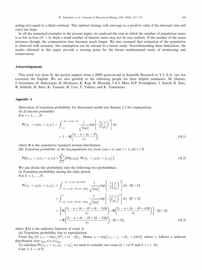
Derivation of transition probability for discretized model (see Section 2.3 for explanation).(I) Extinction probability

For i ¼ 1;y;N:

Pr x�t ¼ y0 xt ¼ yi; etj� �

¼Z � %yi�aþfet�yð Þ

�N

1ffiffiffiffiffiffiffiffiffiffi2ps2

x

q exp �1

2

x

sx

� �2" #

dx

¼ 1� F%yi � a þ fet � y

sx

� �; ðA:1Þ

where F is the cumulative standard normal distribution.(II) Transition probability of the log-population size from year t to year t þ 1; for s > 0;

Pr xtþ1 ¼ ys xt ¼ yi; etj½ � ¼XN

k¼1

Pr ysjyk½ � � Pr x�t ¼ yk xt ¼ yi; etj� � �

: ðA:2Þ

We can divide this probability into the following two probabilities.(i) Transition probability during the risky period.For k ¼ 1;y;N:

Pr x�t ¼ yk xt ¼ yi; etj� �

¼Z � %yi�aþfet�ðyþkDÞf g

� %yi�aþfet�ðyþ k�1ð ÞDÞf g


x

q exp �1

2

x

sx

� �2" #

dx � I i > k½ �

þZ

N

� %yi�aþfet� yþ k�1ð ÞDð Þf g


x

q exp �1

2

x

sx

� �2" #

dx � I i ¼ k½ �

¼ F%yi � a þ fet � ðyþ k � 1ð ÞDÞ

sx

� ��F

%yi � a þ fet � ðyþ kDÞsx

� �� I i > k½ �

þ F%yi � a þ fet � yþ k � 1ð ÞDð Þ

sx

� �� I i ¼ k½ �; ðA:3Þ

where I[A] is the indicator function of event A.(ii) Transition probability due to reproduction.From Eq. (3) ztþ1 ¼ ln rt=bd

� �þ 1� dð Þz�t : Hence rt ¼ exp ztþ1 � z�t þ dz�t þ d ln b

� �where rt follows a uniform

distribution over rminprtprmax:To calculate Pr xtþ1 ¼ ykþsjz�t ¼ yk

� �; we need to consider two cases (k þ saN and k þ s ¼ N):

Case 1: k þ saN:


(a)

Pr xtþ1 ¼ ykþsjx�t ¼ yk

� �¼ 0

for rmaxoexp s �1

2

� �Dþ d %yk þ d ln b

� �or rmin > exp s þ

1

2


� �; ðA:4aÞ

(b)


� �¼

min rmax; exp s þ1

2


� ��

�max rmin; exp s �1

2


� �� 26664

37775�

1

rmax � rminð ÞðA:4bÞ

otherwise.Case 2:k þ s ¼ N :(a)


� �¼ 0

for rmaxoexp s �1

2


� �; ðA:4cÞ

(b)


� �¼

rmax

�max rmin; exp s �1

2


� �� 24

35�

1

rmax � rminð ÞðA:4dÞ

otherwise.(III) Distribution of the cue value

We denote the stochastic variable of the cue in a year t by Ht:

Pr Htþ1 ¼ Zj;Pt; et;mtþ1

h i¼XN

k¼1

XN

i¼1

Pr xtþ1 ¼ yk4Htþ1 ¼ Zj xt ¼ yi; et;mtþ1jh i

pi

¼XN

k¼1

XN

i¼1

Pr Htþ1 ¼ Zj xtþ1 ¼ yk;mtþ1jh in

Pr xtþ1 ¼ yk xt ¼ yi; etj½ �pig: ðA:5Þ

(IV) Posterior probability of the population size given the cue

Pr xtþ1 ¼ yk Htþ1 ¼ Zj;Pt; et;mtþ1

��h i¼

PNi¼1 Pr xtþ1 ¼ yk4Htþ1 ¼ Zj xt ¼ yi; et;mtþ1j

h ipi

Pr Htþ1 ¼ Zj;Pt; et;mtþ1

h i ; ðA:6Þ

where the numerator is as given under III.

Appendix B. Optimal conservation strategy over multiple years

The criterion for the optimization is

F ¼ mine1;y;eTX0

E wXT

t¼1

bt�1u tð Þw x�1 ay0;y; x�t�1ay0; x�t ¼ y0

� �þce

XT

t¼1

bt�1et

��P1

#;

"ðB:1Þ

where w is the indicator function which is 1 if the condition in the brackets is satisfied and 0 otherwise. We introducethe expected future total cost:

V Pt; t½ � ¼ minet;y;eTX0

E wXT

t¼t

bt�tu tð Þ

"w x�t ay0;y;x�t�1ay0;x

�t ¼ y0

� �þce

XT

t¼t

bt�tet

��Pt

#: ðB:2Þ


This can be rewritten as

¼ minetX0

E wu tð Þw x�t ¼ y0

� �þ ceet

��Pt

� �þRPr Ptþ1 Pt; etj½ �

�b minetþ1;y;eTX0

E

wPT

t¼tþ1

bt� tþ1ð Þu tð Þw x�tþ1ay0;y;x�t�1ay0;x�t ¼ y0

� �

þce

PTt¼tþ1

bt� tþ1ð Þet

��Ptþ1

26664

37775 dPtþ1

8>>>>>><>>>>>>:

9>>>>>>=>>>>>>;

¼ minetX0

fwuðtÞPrðx�t ¼ y0jPt; etÞ þ ceet þ bZPr½Ptþ1jPt; et� � V ½Ptþ1; t þ 1� dPtþ1g: ðB:3Þ

In the last expression of Eq. (B.3), the first and the second terms within the brackets are the cost of extinction and thecost of conservation effort in the year t: The third term indicates the total cost after the year t: Eq. (B.3) can berewritten as Eq. (9) in the text.

References

Berger, J.O., 1985. Statistical Decision Theory and Bayesian Analysis 2nd Edition. Springer, New York.

Bosetti, V., Pearce, D., 2003. Study of environmental conflict: the economic value of grey seals in southwest England. Biodivers. Conserv. 12,

2361–2392.

Costanza, R., dArge, R., deGroot, R., Farber, S., Grasso, M., Hannon, B., Limburg, K., Naeem, S., O’Neill, R.V., Paruelo, J., Raskin, R.G., Sutton,

P., van den Belt, M., 1997. The value of the world’s ecosystem services and natural capital. Nature 387, 253–260.

Dorazio, R.M., Johnson, F.A., 2003. Bayesian inference and decision theory—a framework for decision making in natural resource management.

Ecol. Appl. 13, 556–563.

Engen, S., Lande, R., Saether, B.E., 1997. Harvesting strategies for fluctuating populations based on uncertain population estimates. J. Theor. Biol.

186, 201–212.

Hassell, M.P., 1975. Density-dependence in single-species populations. J. Anim. Ecol. 44, 283–295.

Haight, R.G., Cypher, B., Kelly, P.A., Phillips, S., Possingham, H.P., Ralls, K., Starfield, A.M., White, P.J., Williams, D., 2002. Optimizing habitat

protection using demographic models of population viability. Conserv. Biol. 16, 1386–1397.

Jakobsson, K.M., Dragun, A.K., 2001. The worth of a possum: valuing species with the contingent valuation method. Environ. Resour. Econ. 19,

211–227.

Ludwig, D., 1996. Uncertainty and the assessment of extinction probabilities. Ecol. Appl. 6, 1067–1076.

Marin, J.M., Diez, R.M., Insua, D.R., 2003. Bayesian methods in plant conservation biology. Biol. Conserv. 113, 379–387.

Matsuda, H., Kaji, K., Uno, H., Hirakawa, H., Saitoh, T., 1999. A management policy for sika deer based on sex-specific hunting. Res. Popul. Ecol.

41, 139–149.

Milner-Gulland, E.J., Akcakaya, H.R., 2001. Sustainability indices for exploited populations. Trends Ecol. Evol. 16, 686–692.

Possingham, H.P., 1996. Decision theory and biodiversity management: how to manage a metapopulation. In: Floyd, R.B., Sheppard, A.W.,

Wellings, P. (Eds.), Frontiers of Population Ecology. CSIRO Publishing, Canberra, Australia, pp. 391–398.

Possingham, H.P., Tuck, G., 1996. Fire management strategies that minimise the probability of population extinction for early and mid-successional

species. In: Fletcher, D., Kavaliers, L., Manly, B.J.F. (Eds.), Statistics in Ecology and Environmental Monitoring 2. University of Otago Press,

Dunedin, pp. 157–167.

Royama, T., 1992. Analytical population dynamics. Chapman & Hall, London, pp. 371.

Shea, K., Possingham, H.P., 2000. Optimal release strategies for biological control agents: an application of stochastic dynamic programming to

population management. J. Appl. Ecol. 37, 77–86.

Taylor, B.L., Wade, P.R., De Master, D.P., Barlow, J., 2000. Incorporating uncertainty into management models for marine mammals. Conserv.

Biol. 14, 1243–1252.

Turpie, J.K., Heydenrych, B.J., Lamberth, S.J., 2003. Economic value of terrestrial and marine biodiversity in the Cape Floristic Region:

implications for defining effective and socially optimal conservation strategies. Biol. Conserv. 112, 233–251.

Wada, P.R., 2000. Bayesian methods in conservation biology. Conserv. Biol. 14, 1308–1316.

Westphal, M.I., Pickett, M., Getz, W.M., Possingham, H.P., 2003. The use of stochastic dynamic programming in optimal landscape reconstruction

for metapopulations. Ecol. Appl. 13, 543–555.

Whittle, P., 1982. Optimization Over Time: Dynamic Programming and Stochastic Control. Vol. II, Wiley, New York.

Yokomizo, H., Yamashita, J., Iwasa, Y., 2003a. Optimal conservation effort for a population in a stochastic environment. J. Theor. Biol. 220,

215–231.

Yokomizo, H., Haccou, P., Iwasa, Y., 2003b. Conservation effort and assessment of population size in fluctuating environments. J. Theor. Biol. 224,

167–182.

multiple-year optimization of conservation effort and monitoring effort for a fluctuating population

Documents