Multiple Regression

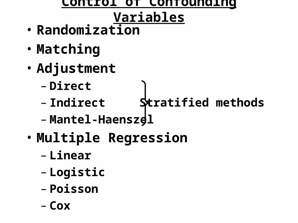
Control of Confounding Variables

• Randomization

• Matching

• Adjustment– Direct– Indirect– Mantel-Haenszel

• Multiple Regression– Linear– Logistic– Poisson– Cox

Stratified methods

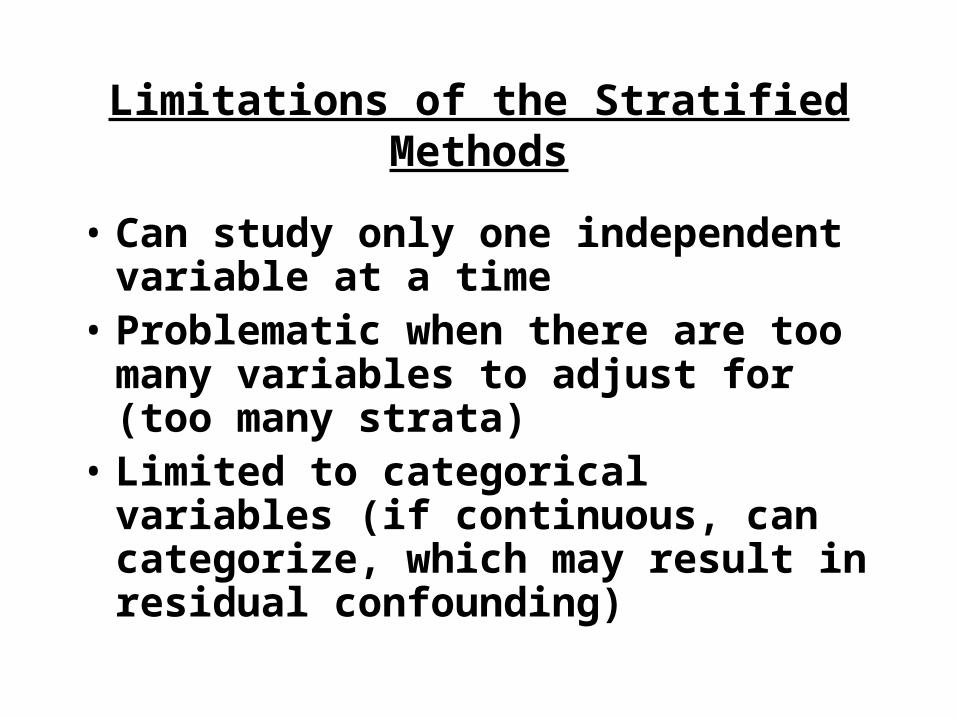
Limitations of the Stratified Methods

• Can study only one independent variable at a time

• Problematic when there are too many variables to adjust for (too many strata)

• Limited to categorical variables (if continuous, can categorize, which may result in residual confounding)

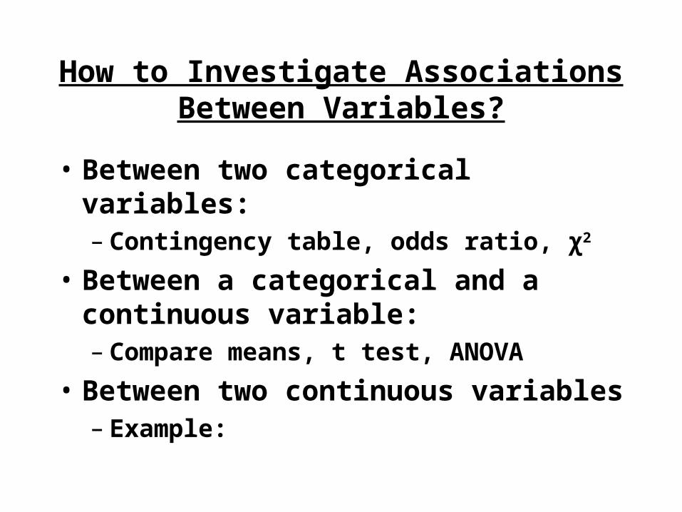
How to Investigate Associations Between Variables?

• Between two categorical variables:– Contingency table, odds ratio, χ2

• Between a categorical and a continuous variable: – Compare means, t test, ANOVA

• Between two continuous variables– Example:

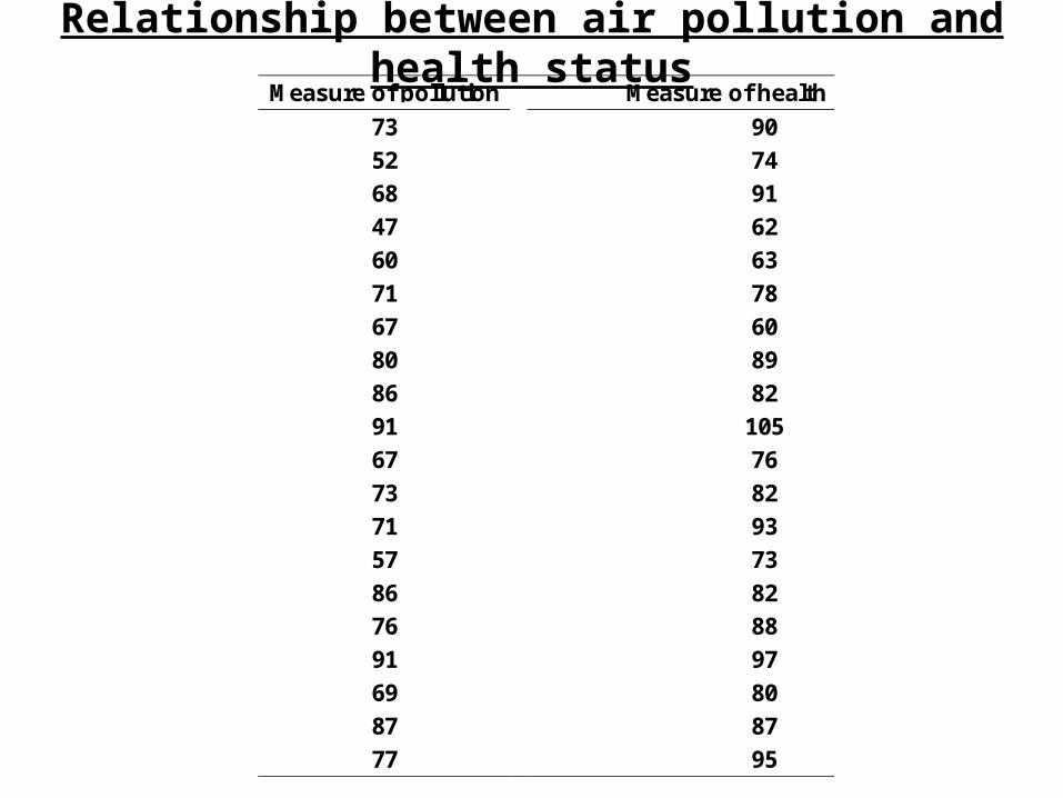
Relationship between air pollution and health statusMeasure of pollution Measure of health status

73 90

52 74

68 91

47 62

60 63

71 78

67 60

80 89

86 82

91 105

67 76

73 82

71 93

57 73

86 82

76 88

91 97

69 80

87 87

77 95

20 40 60 80 100 1200

20

40

60

80

100

120

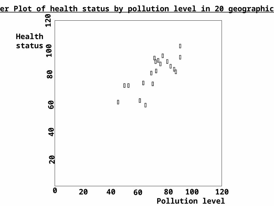
Scatter Plot of health status by pollution level in 20 geographic areas

Pollution level

Healthstatus

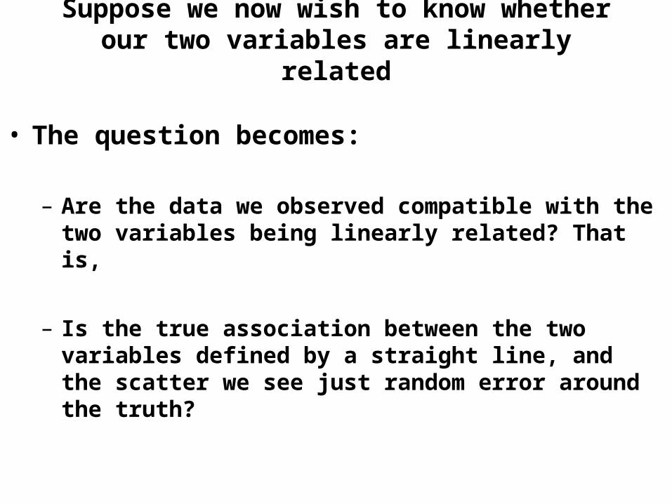
Suppose we now wish to know whether our two variables are linearly related

• The question becomes:

– Are the data we observed compatible with the two variables being linearly related? That is,

– Is the true association between the two variables defined by a straight line, and the scatter we see just random error around the truth?

20 40 60 80 100 1200

20

40

60

80

100

120

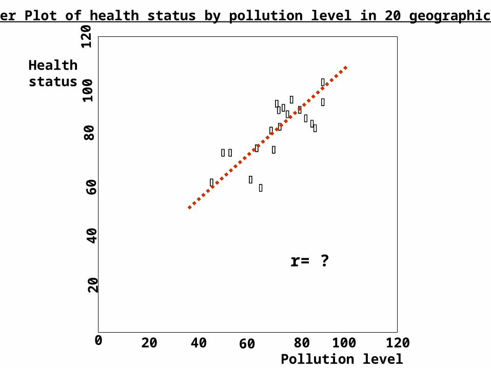
Scatter Plot of health status by pollution level in 20 geographic areas

Pollution level

Healthstatus

r= ?

20 40 60 80 100 1200

20

40

60

80

100

120

Scatter Plot of health status by pollution level in 20 geographic areas

Pollution level

Healthstatus

r0.7

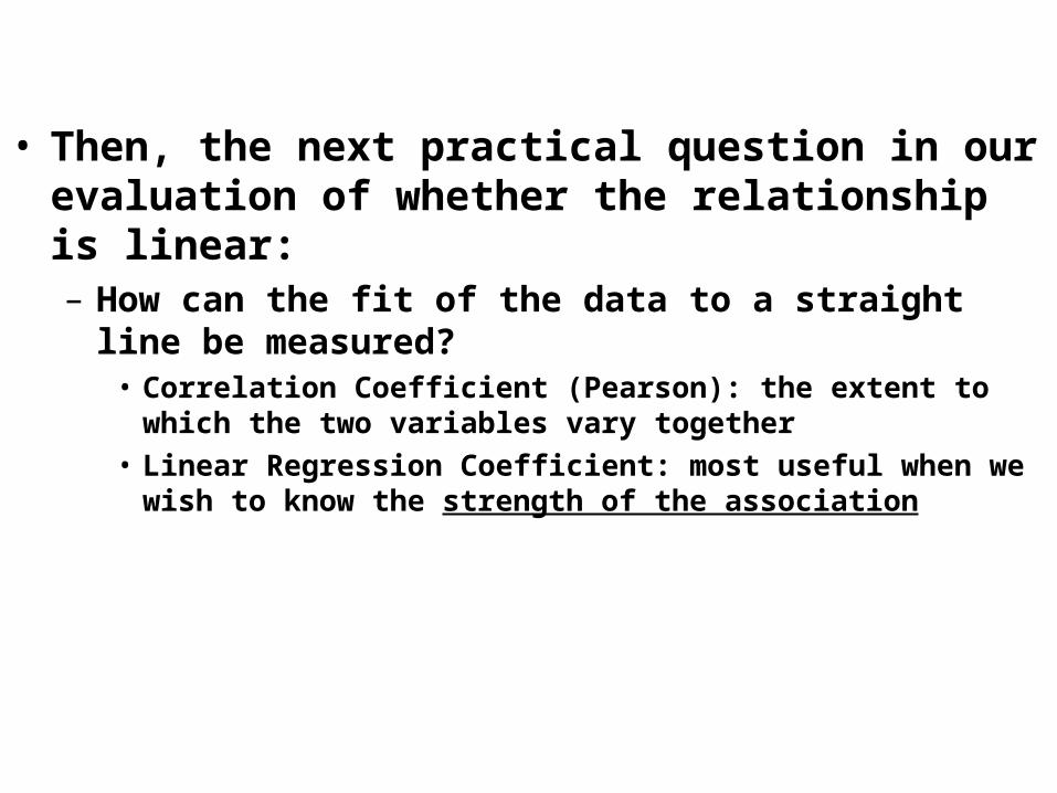
• Then, the next practical question in our evaluation of whether the relationship is linear:– How can the fit of the data to a straight line be

measured?• Correlation Coefficient (Pearson): the extent to which the two

variables vary together• Linear Regression Coefficient: most useful when we wish to

know the strength of the association

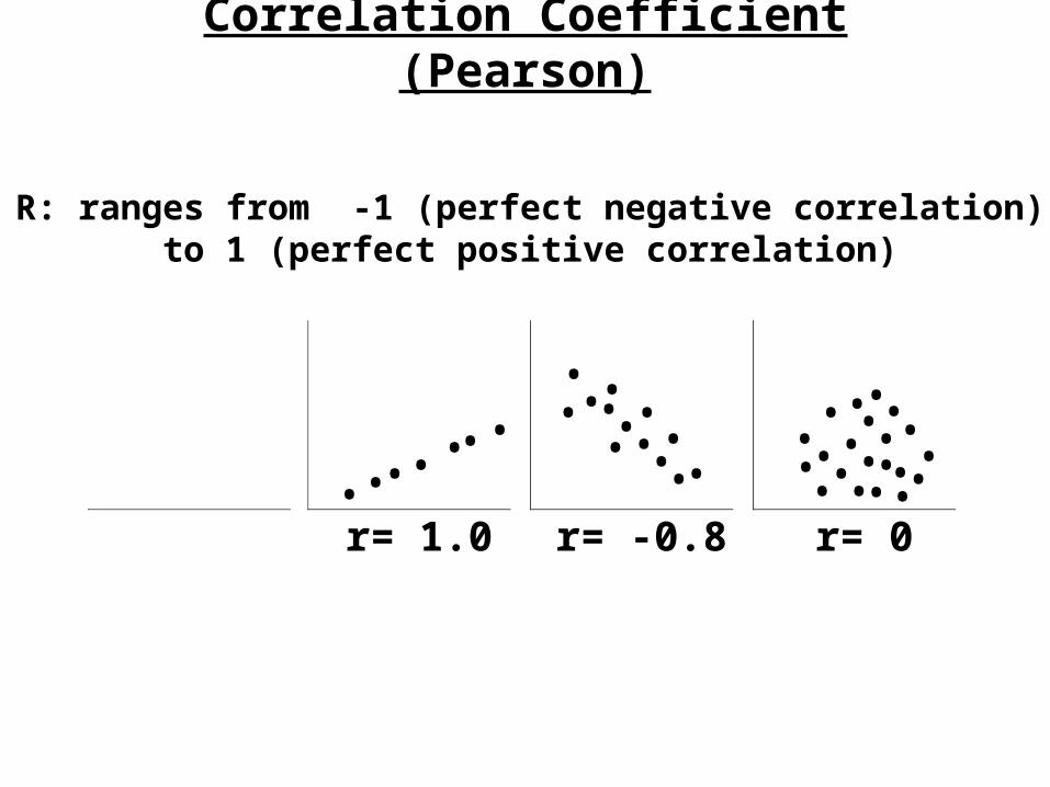
Correlation Coefficient (Pearson)

r= 1.0 r= -0.8 r= 0

R: ranges from -1 (perfect negative correlation) to 1 (perfect positive correlation)

•••

••

•

•

• • • • • • •

•• •

•

••

• • • •

••••• •• •

• ••

•••

•

• •

Linear Regression Coefficient of a Straight Line

1 unit

0

1

y

0

x= 0, y= 0

1 Linear regression coefficient: increase in y per unit increase in x: expresses strength of the association: allows prediction of the value of y, given x

y x 0 1

x

20 40 60 80 100 1200

20

40

60

80

100

120

X= Pollution level

Y= Healthstatus

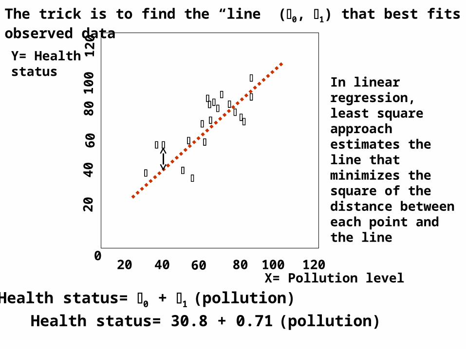
The trick is to find the “line” (0, 1) that best fits the observed data

Health status= 0 + 1 (pollution)

Health status= 30.8 + 0.71 (pollution)

In linear regression, least square approach estimates the line that minimizes the square of the distance between each point and the line

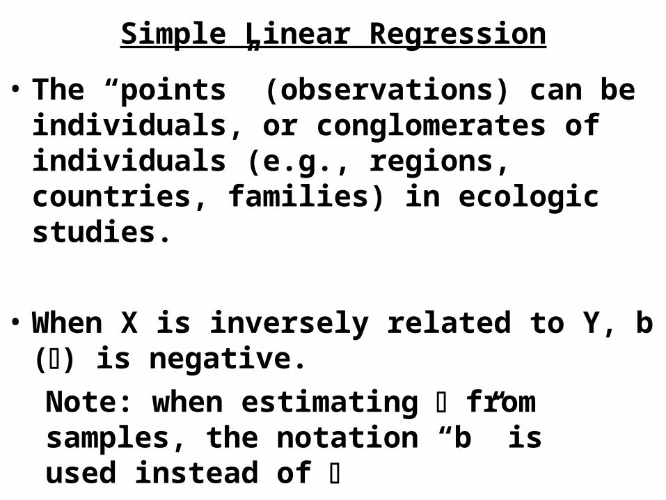
Simple Linear Regression

• The “points” (observations) can be individuals, or conglomerates of individuals (e.g., regions, countries, families) in ecologic studies.

• When X is inversely related to Y, b () is negative.

Note: when estimating from samples, the notation “b” is used instead of

• In epidemiologic studies, the value of the intercept (b0 or 0) is frequently irrelevant (X=0 is meaningless for many variables)– E.g. Relationship of weight (X) to systolic blood

pressure (Y):

0100 150 200

WEIGHT (Lb)

SBP(mmHg)

100

200

50?

••

•

•••

••

•

••

•

•

•• •

•

•

••

•

•

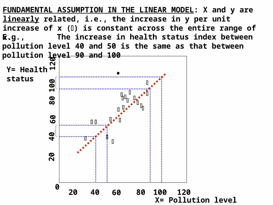
FUNDAMENTAL ASSUMPTION IN THE LINEAR MODEL: X and y are linearly related, i.e., the increase in y per unit increase of x () is constant across the entire range of x.E.g., The increase in health status index between pollution level 40 and 50 is the same as that between pollution level 90 and 100

•

20 40 60 80 100 1200

20

40

60

80

100

120

X= Pollution level

Y= Healthstatus

FUNDAMENTAL ASSUMPTION IN THE LINEAR MODEL:

X and y are linearly related

However…if the data look like this:

• • • ••

••

•• • •

••

•

•••

••

••

•

••• ••

•

x

y

•“u-shaped” function

Wrong model!

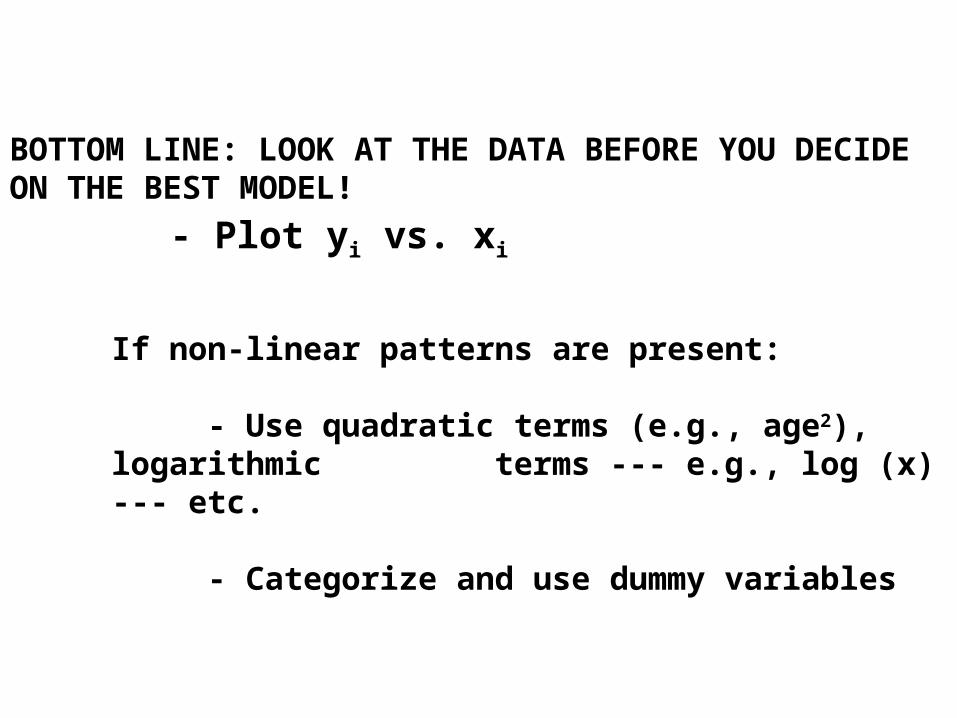
BOTTOM LINE: LOOK AT THE DATA BEFORE YOU DECIDE ON THE BEST MODEL!

If non-linear patterns are present:

- Use quadratic terms (e.g., age2), logarithmic terms --- e.g., log (x) --- etc.

- Categorize and use dummy variables

- Plot yi vs. xi

Other important points to keep in mind

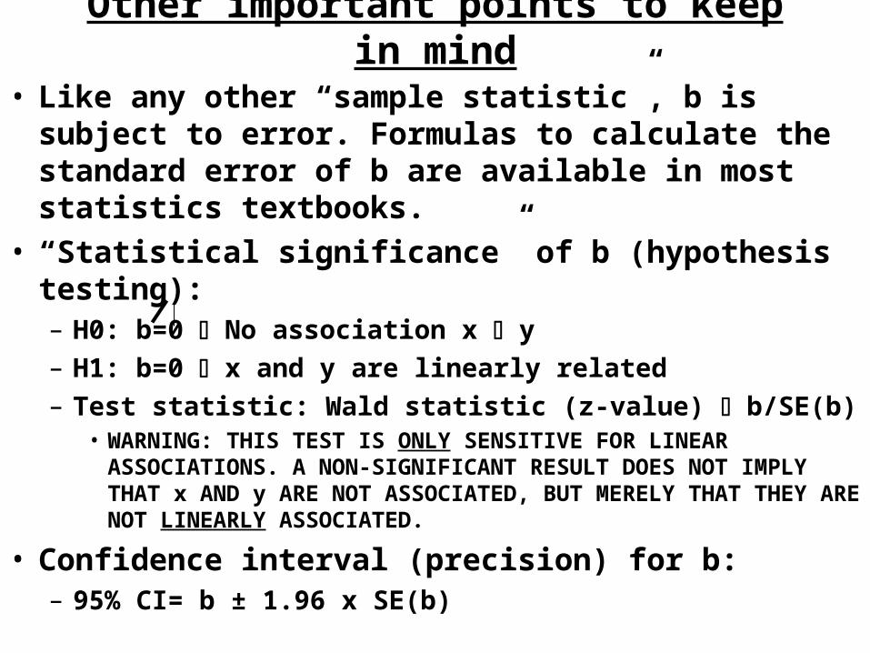
• Like any other “sample statistic”, b is subject to error. Formulas to calculate the standard error of b are available in most statistics textbooks.

• “Statistical significance” of b (hypothesis testing):– H0: b=0 No association x y– H1: b=0 x and y are linearly related– Test statistic: Wald statistic (z-value) b/SE(b)

• WARNING: THIS TEST IS ONLY SENSITIVE FOR LINEAR ASSOCIATIONS. A NON-SIGNIFICANT RESULT DOES NOT IMPLY THAT x AND y ARE NOT ASSOCIATED, BUT MERELY THAT THEY ARE NOT LINEARLY ASSOCIATED.

• Confidence interval (precision) for b:– 95% CI= b ± 1.96 x SE(b)

• The regression coefficient (b) is related to the correlation coefficient (r), but the former is generally preferable because:

– It gives some sense of the strength of the association, not only the extent to each two variables vary concurrently in a linear fashion.

– It allows prediction of Y as a function of X.

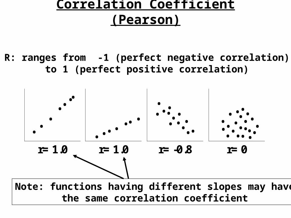
Correlation Coefficient (Pearson)

r= 1.0 r= 1.0 r= -0.8 r= 0

R: ranges from -1 (perfect negative correlation) to 1 (perfect positive correlation)

• •

•

•

••

•

•••

••

•

•

• • • • • • •

•• •

•

••

• • • •

••••• •• •

• ••

•••

•

• •

Note: functions having different slopes may havethe same correlation coefficient

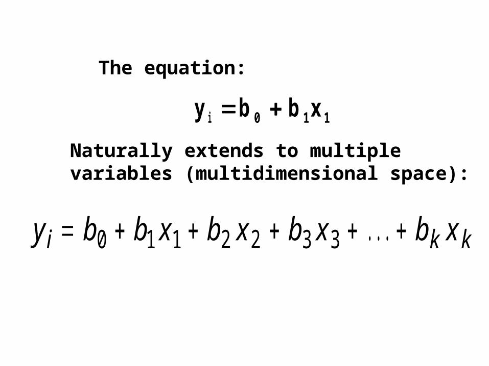
y b b xi 0 1 1

The equation:

Naturally extends to multiple variables (multidimensional space):

y b b x b x b x b xi k k 0 1 1 2 2 3 3 . . .

x1

y

x2

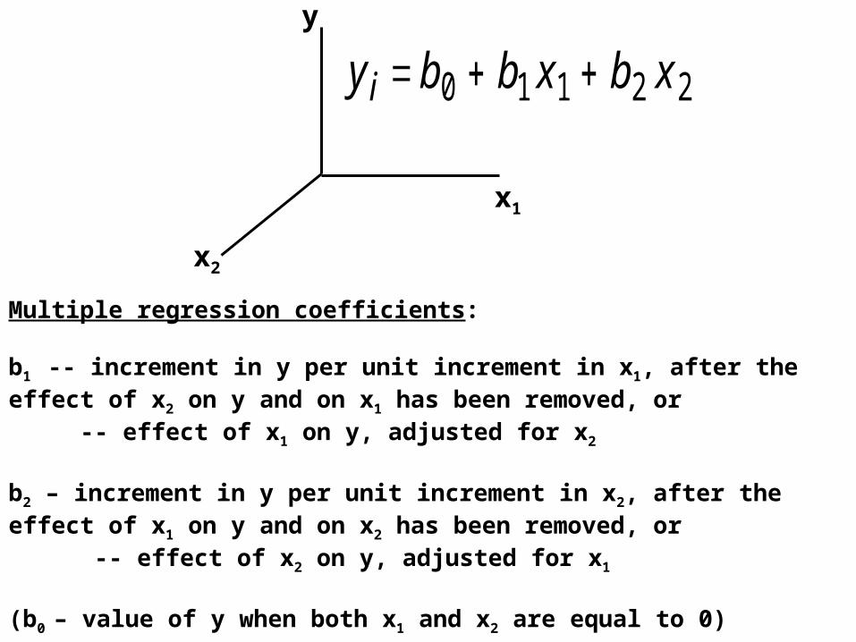
y b b x b xi 0 1 1 2 2

Multiple regression coefficients:

b1 -- increment in y per unit increment in x1, after the effect of x2 on y and on x1 has been removed, or -- effect of x1 on y, adjusted for x2

b2 – increment in y per unit increment in x2, after the effect of x1 on y and on x2 has been removed, or -- effect of x2 on y, adjusted for x1

(b0 – value of y when both x1 and x2 are equal to 0)

y b b x b x e

y b b x b x e

osed

un osed

exp

exp

0 1 1 2 2

0 1 1 2 2

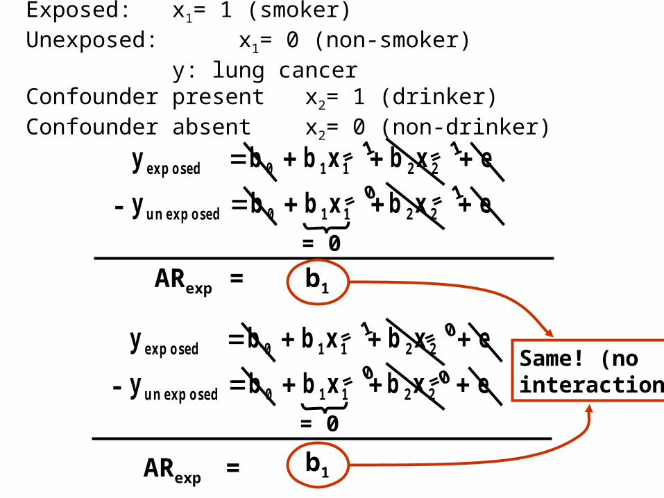
Exposed: x1= 1 (smoker)Unexposed: x1= 0 (non-smoker)

y: lung cancerConfounder present x2= 1 (drinker)Confounder absent x2= 0 (non-drinker)

-

= 1

= 0

= 0

= 1

= 1

ARexp = b1

= 0

=0

y b b x b x e

y b b x b x e

osed

un osed

exp

exp

0 1 1 2 2

0 1 1 2 2-

= 1

= 0

= 0

ARexp = b1

Same! (nointeraction)

x1

y

x2

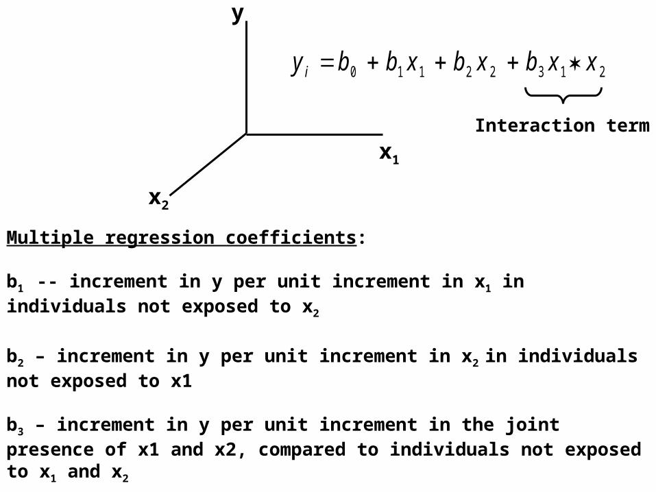
y b b x b x b x xi 0 1 1 2 2 3 1 2

Multiple regression coefficients:

b1 -- increment in y per unit increment in x1 in individuals not exposed to x2

b2 – increment in y per unit increment in x2 in individuals not exposed to x1

b3 – increment in y per unit increment in the joint presence of x1 and x2, compared to individuals not exposed to x1 and x2

Interaction term

Multiple Linear Regression Notes

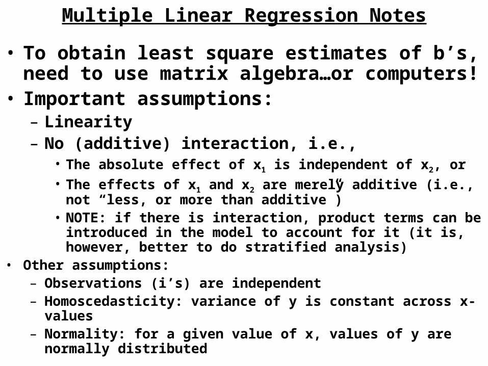
• To obtain least square estimates of b’s, need to use matrix algebra…or computers!

• Important assumptions:– Linearity– No (additive) interaction, i.e.,

• The absolute effect of x1 is independent of x2, or• The effects of x1 and x2 are merely additive (i.e., not “less, or

more than additive”)• NOTE: if there is interaction, product terms can be introduced in

the model to account for it (it is, however, better to do stratified analysis)

• Other assumptions:– Observations (i’s) are independent– Homoscedasticity: variance of y is constant across x-values– Normality: for a given value of x, values of y are normally

distributed

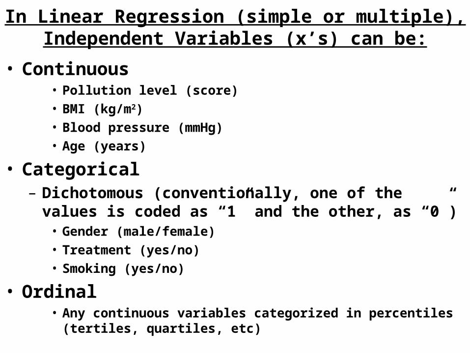
In Linear Regression (simple or multiple), Independent Variables (x’s) can be:

• Continuous• Pollution level (score)• BMI (kg/m2)• Blood pressure (mmHg)• Age (years)

• Categorical– Dichotomous (conventionally, one of the values is

coded as “1” and the other, as “0”)• Gender (male/female)• Treatment (yes/no)• Smoking (yes/no)

• Ordinal• Any continuous variables categorized in percentiles (tertiles,

quartiles, etc)

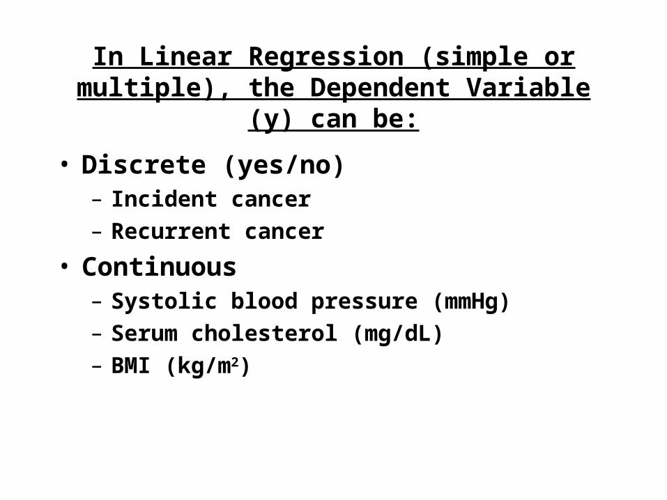
• Discrete (yes/no)– Incident cancer– Recurrent cancer

• Continuous– Systolic blood pressure (mmHg)– Serum cholesterol (mg/dL)– BMI (kg/m2)

In Linear Regression (simple or multiple), the Dependent Variable (y) can be:

Example of x as a discrete variable (obesity) and y as a continuous variable (systolic blood pressure, mmHg)

0 1

Obesity (x= 0 if “no”; x=1 if “yes”)

110

120

130

140

150

160

SBP b b b b 0 1 0 11When x= 1,

SBP b b b 0 1 00When x= 0,

Thus, b1 = increase in SBP per unit increase in obesity = average difference in SBP between “obese” and “non-obese” individuals

-SBP = b1

Unit: from zero to 1

Average difference(regression coefficient or slope = b1)

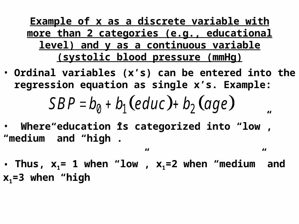
• Ordinal variables (x’s) can be entered into the regression equation as single x’s. Example:

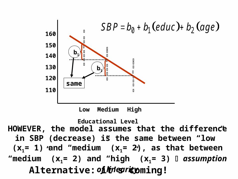
Example of x as a discrete variable with more than 2 categories (e.g., educational level) and y as a continuous variable (systolic blood pressure

(mmHg)

SBP b b educ b age 0 1 2• Where education is categorized into “low”, “medium” and “high”.

• Thus, x1= 1 when “low”, x1=2 when “medium” and x1=3 when “high”

110

120

130

140

150

160

Low Medium High

Educational Level

SBP b b educ b age 0 1 2

HOWEVER, the model assumes that the difference in SBP (decrease) is the same between “low” (x1= 1) and

“medium” (x1= 2), as that between “medium” (x1= 2) and “high” (x1= 3) assumption of linearity

b1

Alternative: it’s coming!

b1

same

Non-ordinal multilevel categorical variable

• Race (Asian, Black, Hispanic, White)• Treatment (A, B, C, D)• Smoking (cigarette, pipe, cigar, nonsmoker)

How to include these variables in a multipleregression model?

“Dummy” or indicator variables: Define the number of dummy dichotomous variables as the number of categories

minus one

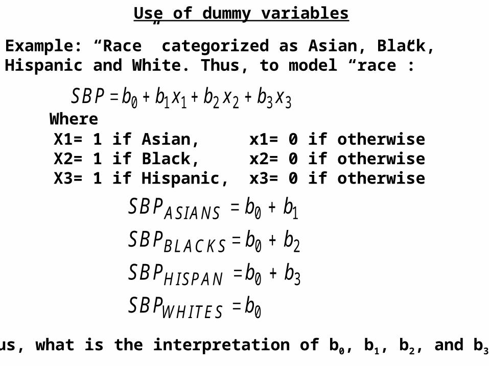
Use of dummy variables

Example: “Race” categorized as Asian, Black, Hispanic and White. Thus, to model “race”:

SBP b b x b x b x 0 1 1 2 2 3 3Where

X1= 1 if Asian, x1= 0 if otherwiseX2= 1 if Black, x2= 0 if otherwiseX3= 1 if Hispanic, x3= 0 if otherwise

SBP b b

SBP b b

SBP b b

SBP b

ASIANS

BLACKS

H ISPAN

WH ITES

0 1

0 2

0 3

0

Thus, what is the interpretation of b0, b1, b2, and b3?

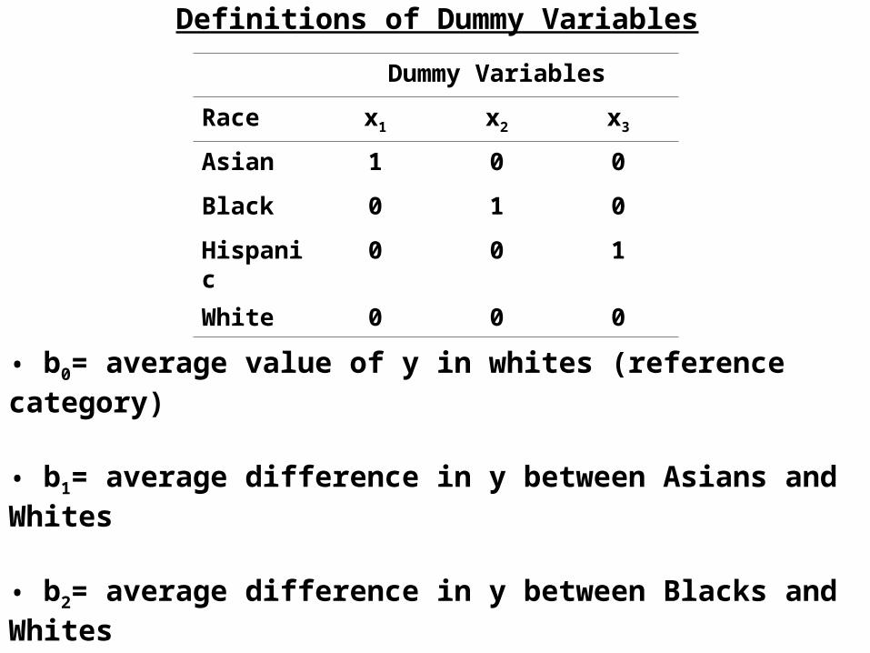
Definitions of Dummy Variables

Dummy Variables

Race x1 x2 x3

Asian 1 0 0

Black 0 1 0

Hispanic 0 0 1

White 0 0 0

• b0= average value of y in whites (reference category)

• b1= average difference in y between Asians and Whites

• b2= average difference in y between Blacks and Whites

• b3= average difference in y between Hispanics and Whites

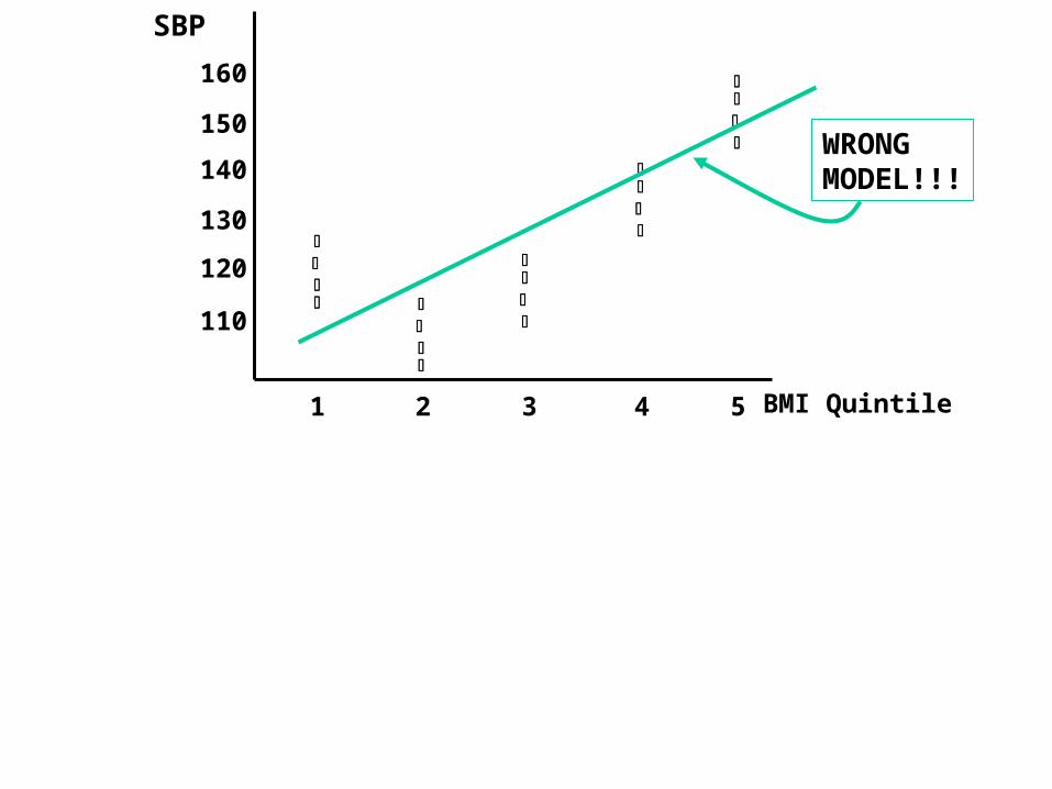
Use of dummy variables when the function is not a straight line

110

120

130

140

150

160

1 2 3 4 5

BMI Quintile

WRONG MODEL!!!

SBP

110

120

130

140

150

160

1 2 3 4 5

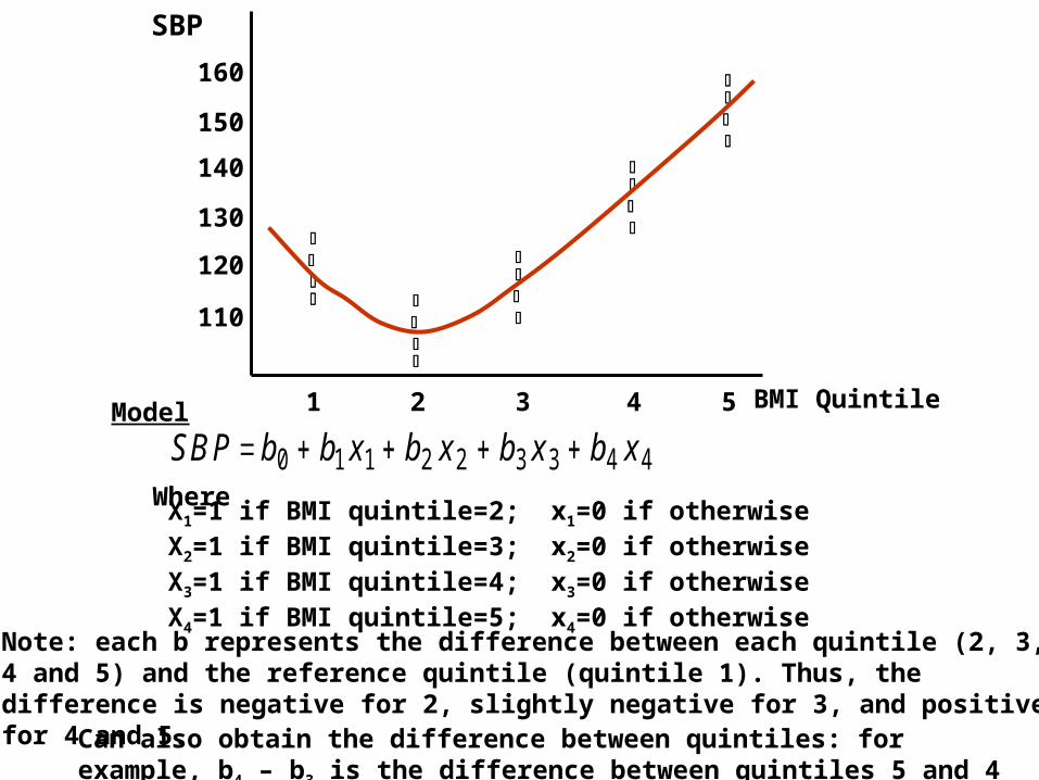
Model

SBP b b x b x b x b x 0 1 1 2 2 3 3 4 4

BMI Quintile

Where X1=1 if BMI quintile=2; x1=0 if otherwiseX2=1 if BMI quintile=3; x2=0 if otherwiseX3=1 if BMI quintile=4; x3=0 if otherwiseX4=1 if BMI quintile=5; x4=0 if otherwise

Note: each b represents the difference between each quintile (2, 3, 4 and 5) and the reference quintile (quintile 1). Thus, the difference is negative for 2, slightly negative for 3, and positive for 4 and 5.

Can also obtain the difference between quintiles: for example, b4 – b3 is the difference between quintiles 5 and 4

SBP

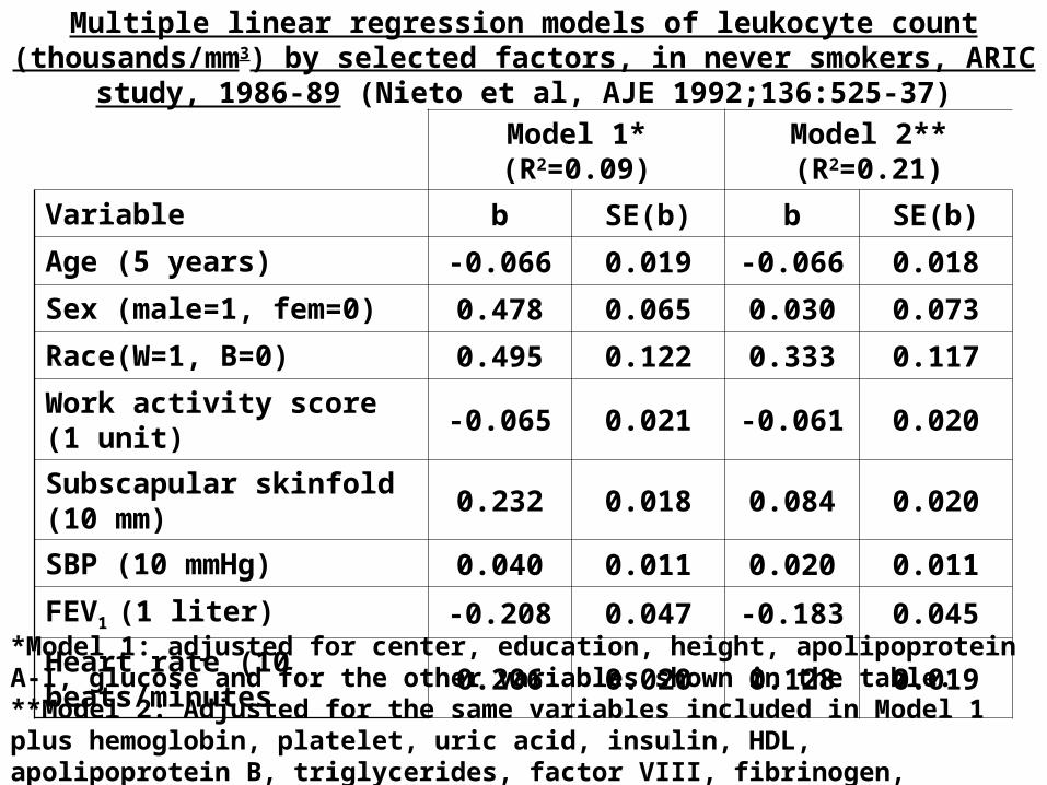
Multiple linear regression models of leukocyte count (thousands/mm3) by selected factors, in never smokers, ARIC study, 1986-89 (Nieto et al, AJE

1992;136:525-37)

Model 1* (R2=0.09) Model 2** (R2=0.21)

Variable b SE(b) b SE(b)

Age (5 years) -0.066 0.019 -0.066 0.018

Sex (male=1, fem=0) 0.478 0.065 0.030 0.073

Race(W=1, B=0) 0.495 0.122 0.333 0.117

Work activity score (1 unit) -0.065 0.021 -0.061 0.020

Subscapular skinfold (10 mm)

0.232 0.018 0.084 0.020

SBP (10 mmHg) 0.040 0.011 0.020 0.011

FEV1 (1 liter) -0.208 0.047 -0.183 0.045

Heart rate (10 beats/minutes 0.206 0.020 0.128 0.019

*Model 1: adjusted for center, education, height, apolipoprotein A-I, glucose and for the other variables shown in the table.**Model 2: Adjusted for the same variables included in Model 1 plus hemoglobin, platelet, uric acid, insulin, HDL, apolipoprotein B, triglycerides, factor VIII, fibrinogen, antithrombin III, protein C antigen and APTT

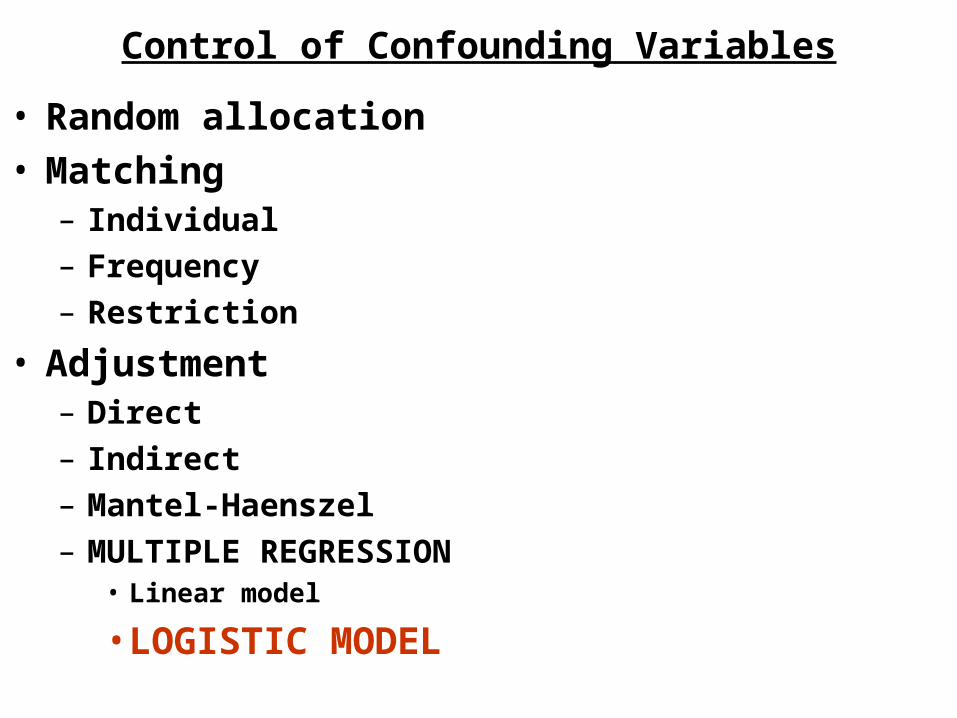
Control of Confounding Variables

• Random allocation• Matching

– Individual– Frequency– Restriction

• Adjustment– Direct– Indirect– Mantel-Haenszel– MULTIPLE REGRESSION

• Linear model

• LOGISTIC MODEL

Dose (x)

0

0.5

1.0

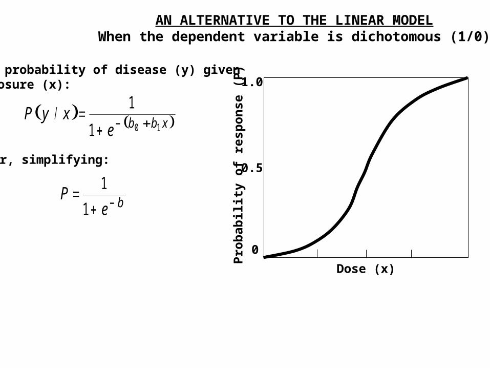
AN ALTERNATIVE TO THE LINEAR MODELWhen the dependent variable is dichotomous (1/0)

P y xe b b x

/

1

1 0 1

The probability of disease (y) givenexposure (x):

Or, simplifying:

Pe b

1

1

Pro

bab

ilit

y o

f re

spo

nse

(P

)

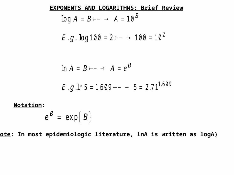
EXPONENTS AND LOGARITHMS: Brief Review

lo g

. . lo g

ln

. . ln . . .

A B A

E g

A B A e

E g

B

B

1 0

1 0 0 2 1 0 0 1 0

5 1 6 0 9 5 2 7 1

2

1 6 0 9

Notation:

e BB ex p

(Note: In most epidemiologic literature, lnA is written as logA)

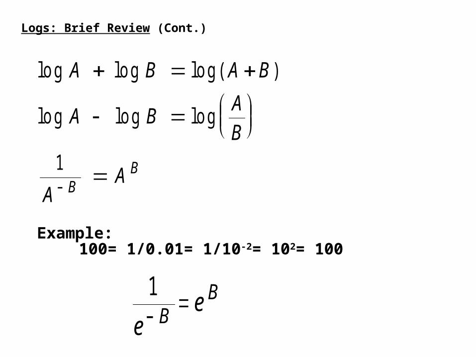
lo g lo g lo g ( )

lo g lo g lo g

A B A B

A BA

B

AA

BB

1

Logs: Brief Review (Cont.)

Example:100= 1/0.01= 1/10-2= 102= 100

1

ee

BB

1 11

1

1 1

1 1

P

e

e

e

e

eB

B

B

B

B

P

P

e B

e B

e Be B

e B1

1

1

1

1

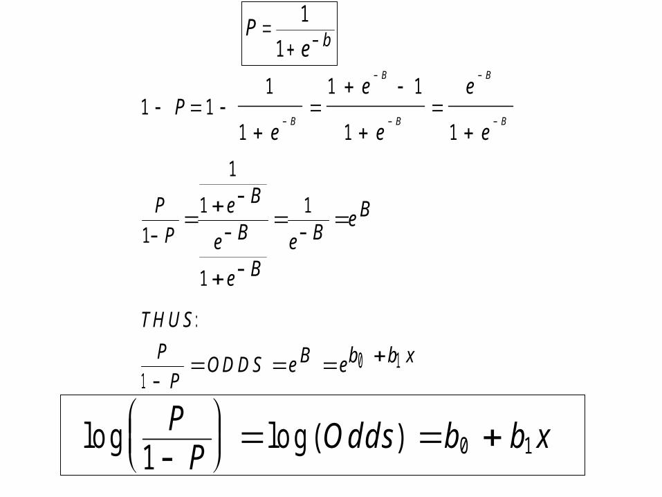
Pe b

1

1

THUS

P

PODDS e B eb b x

:

10 1

lo g lo g ( )PP

O dds b b x1 0 1

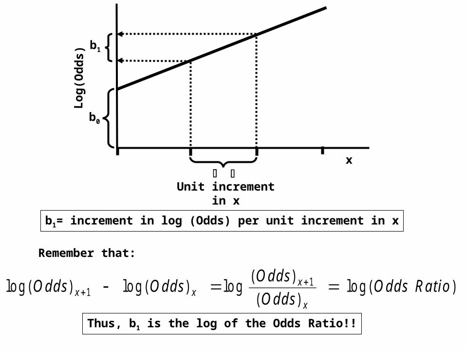
b0

x

b1

Unit incrementin x

b1= increment in log (Odds) per unit increment in x

Lo

g(O

dd

s)

lo g ( ) lo g ( ) lo g( )

( )lo g ( )Odds O dds

O dds

O ddsO dds Ra tiox x

x

x

11

Remember that:

Thus, b1 is the log of the Odds Ratio!!

Assume prospective data in which exposure (independent variable) is defined dichotomously (x):

Disease Non disease

Y=1 Y=0

Exposed X=1 p1 1 – p1

Unexposed X=0 P0 1 – p0

lo gPP

b b x b b1

10 1 0 11

1

For exposed (x=1):

lo gPP

b b b0

00 1 01

0

For unexposed (x=0):

bP

P

P

P

P

PP

P

OR11

1

0

0

1

1

0

0

1 1

1

1

lo g lo g lo g lo g

OR e An ti o f bb 11lo g

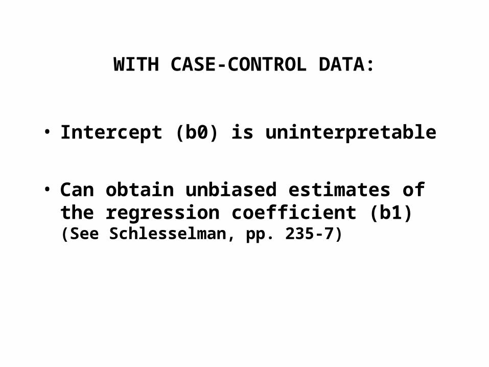
WITH CASE-CONTROL DATA:

• Intercept (b0) is uninterpretable

• Can obtain unbiased estimates of the regression coefficient (b1) (See Schlesselman, pp. 235-7)

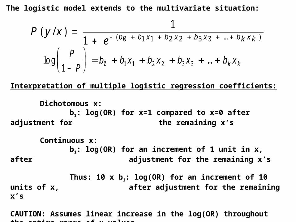
The logistic model extends to the multivariate situation:

P y xe b b x b x b x b k x k

( / )( ... )

1

1 0 1 1 2 2 3 3

lo g ...P

Pb b x b x b x b xk k1 0 1 1 2 2 3 3

Interpretation of multiple logistic regression coefficients:

Dichotomous x:b1: log(OR) for x=1 compared to x=0 after adjustment for the remaining x’s

Continuous x:b1: log(OR) for an increment of 1 unit in x, after adjustment for the remaining x’s

Thus: 10 x b1: log(OR) for an increment of 10 units of x, after adjustment for the remaining x’s

CAUTION: Assumes linear increase in the log(OR) throughout the entire range of x values

Logistic Regression Using Dummy Variables: Cross-Sectional Association Between Demographic Factors and Depressive State, NHANES, Mexican-

Americans Aged 20-74 Years, 1982-4

Factor b OR P value

Intercept -3.1187 - -

Sex (female= 1, male= 0) 0.8263 2.28 0.00

Age

20-24 Reference 1.00 -

25-34 0.1866 1.20 0.11

35-44 -0.1112 0.89 0.60

45-54 -0.1264 0.88 0.52

55-64 -0.1581 0.85 0.32

65-74 -0.3555 0.70 0.19

Years of Education

0-6 0.8408 2.32 0.00

7-11 0.4470 1.56 0.01

12 0.2443 1.28 0.21

13 Reference 1.00 -

Generalized Linear Models

Model Equation Interpretation

Linear (simple) Increase in outcome y mean value per unit increase in x1, adjusted for all other variables in model

Logistic Increase in log (odds) of outcome per unit increase in x1, adjusted for all other variables in model

Cox Increase in log (hazard) of outcome per unit increase in x1, adjusted for all other variables in model

Poisson Increase in log (hazard) of outcome per unit increase in x1, adjusted for all other variables in model

y b b x b x b xk k 0 1 1 2 2 . . .

Log odds b b x b x b xk k( ) . . . 0 1 1 2 2

Log hazard b b x b x b xk k( ) . . . 0 1 1 2 2

Log ra te b b x b x b xk k( ) . . . 0 1 1 2 2

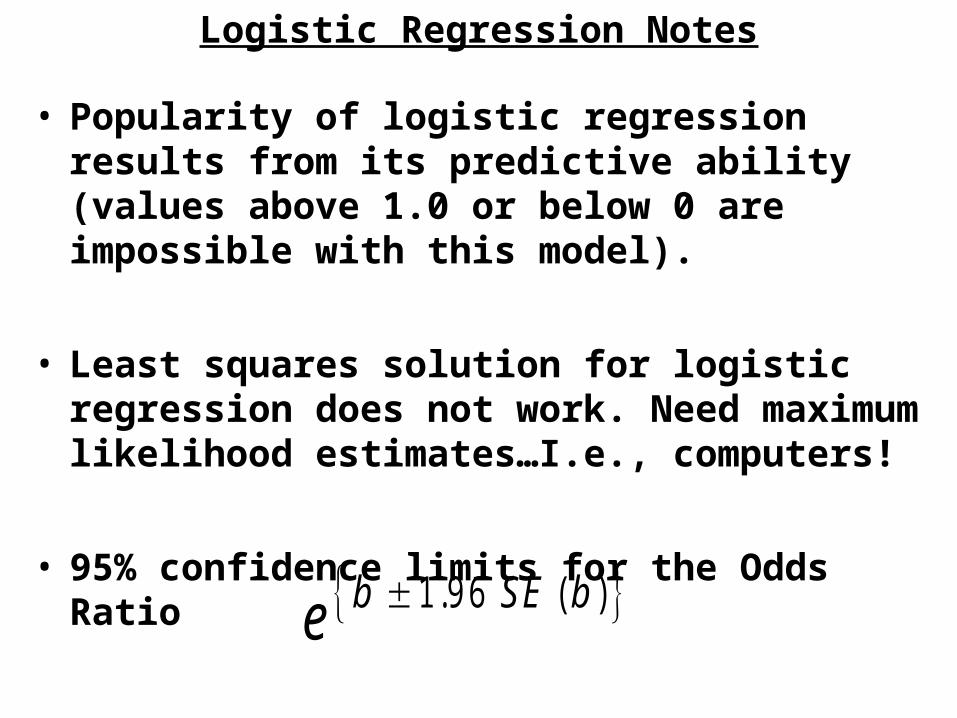
Logistic Regression Notes

• Popularity of logistic regression results from its predictive ability (values above 1.0 or below 0 are impossible with this model).

• Least squares solution for logistic regression does not work. Need maximum likelihood estimates…I.e., computers!

• 95% confidence limits for the Odds Ratio

e b SE b1 9 6. ( )

Logistic Regression on 7-Year Follow-Up, Washington County ARIC Cohort, Ages 45-64 Years at Baseline (1987-89)

Factor (x) b Odds Ratio

Intercept -4.5670 -

Gender (male=1, female=0)

1.3106 3.71

Smoking (yes=1, no=0) 0.7030 2.02

Age (1 year) 0.1444 1.16

Systolic Blood Pressure (1 mmHg)

0.5103 1.67

Serum Cholesterol (1 mg/dL)

0.4916 1.63

Body Mass Index (1 kg/m2)

0.1916 1.21

What is the probability (P) that can be predicted from this model for a male smoker less than 55 years old, who is hypertensive, non-hypercholesterolemic and obese?

PO dds

O dds

1

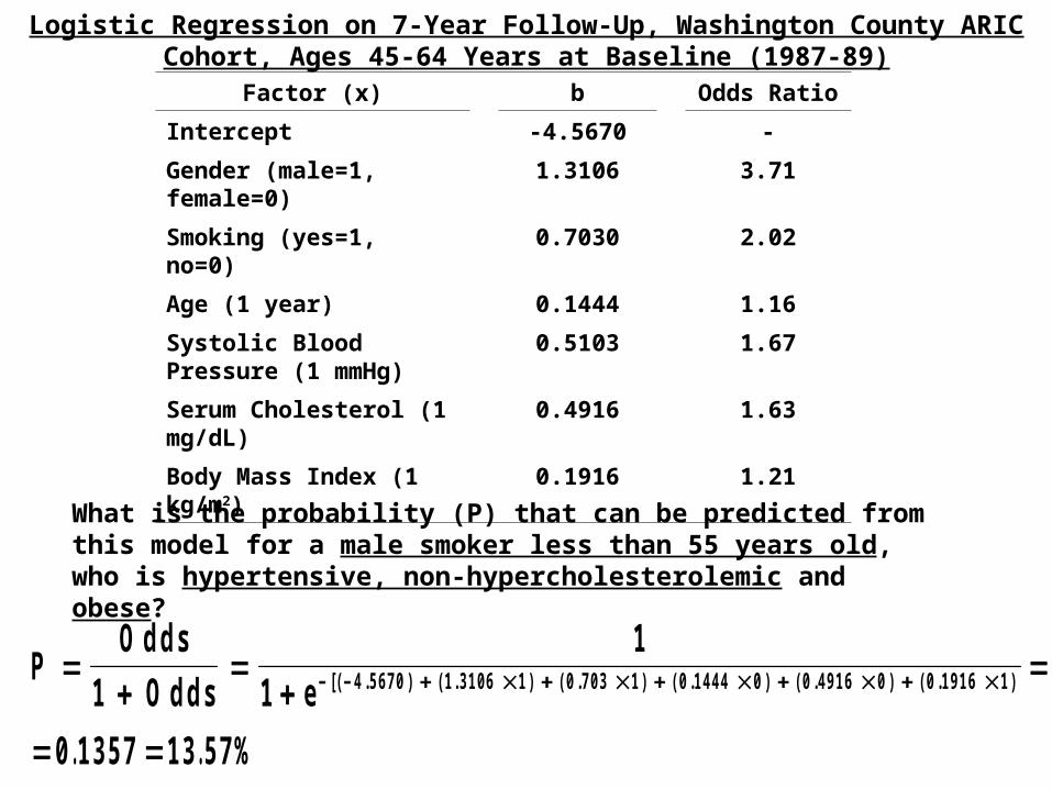
Logistic Regression on 7-Year Follow-Up, Washington County ARIC Cohort, Ages 45-64 Years at Baseline (1987-89)

Factor (x) b Odds Ratio

Intercept -4.5670 -

Gender (male=1, female=0)

1.3106 3.71

Smoking (yes=1, no=0) 0.7030 2.02

Age (1 year) 0.1444 1.16

Systolic Blood Pressure (1 mmHg)

0.5103 1.67

Serum Cholesterol (1 mg/dL)

0.4916 1.63

Body Mass Index (1 kg/m2)

0.1916 1.21

What is the probability (P) that can be predicted from this model for a male smoker less than 55 years old, who is hypertensive, non-hypercholesterolemic and obese?

PO dds

O dds e

1

1

1

0 1357 13 57%

4 5670 1 3106 1 0 703 1 0 1444 0 0 4916 0 0 1916 1[( . ) ( . ) ( . ) ( . ) ( . ) ( . )

. .

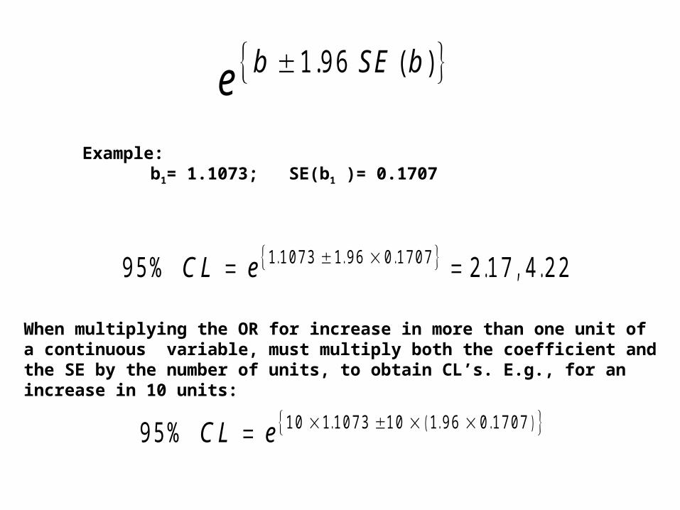
e b SE b1 9 6. ( )

Example: b1= 1.1073; SE(b1 )= 0.1707

9 5 % 2 1 7 4 2 21 1 07 3 1 9 6 0 1 70 7CL e . . . . , .

When multiplying the OR for increase in more than one unit of a continuous variable, must multiply both the coefficient and the SE by the number of units, to obtain CL’s. E.g., for an increase in 10 units:

9 5 % 1 0 1 1 0 7 3 1 0 1 9 6 0 1 7 0 7CL e . ( . . )

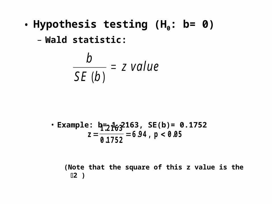
• Hypothesis testing (H0: b= 0)– Wald statistic:

• Example: b= 1.2163, SE(b)= 0.1752

(Note that the square of this z value is the 2 )

b

SE bz va lue

( )

z p 1 2163

0 17526 94 0 05

.

.. , .

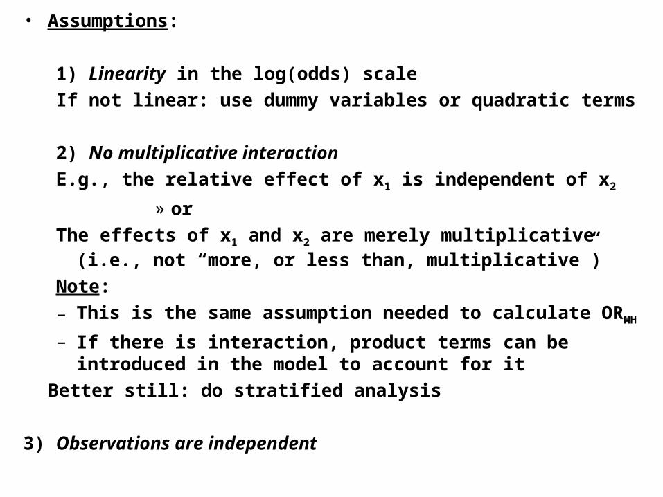
• Assumptions:

1) Linearity in the log(odds) scale

If not linear: use dummy variables or quadratic terms

2) No multiplicative interaction

E.g., the relative effect of x1 is independent of x2

» or

The effects of x1 and x2 are merely multiplicative (i.e., not “more, or less than, multiplicative”)

Note:

– This is the same assumption needed to calculate ORMH

– If there is interaction, product terms can be introduced in the model to account for it

Better still: do stratified analysis

3) Observations are independent

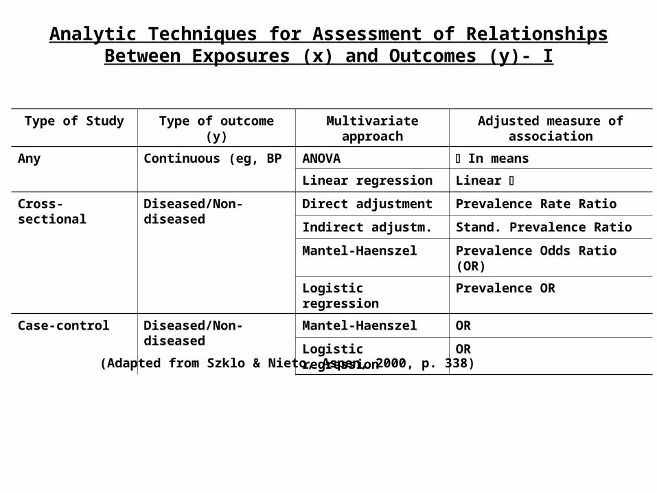
Analytic Techniques for Assessment of Relationships Between Exposures (x) and Outcomes (y)- I

Type of Study Type of outcome (y) Multivariate approach Adjusted measure of association

Any Continuous (eg, BP ANOVA In means

Linear regression Linear

Cross-sectional Diseased/Non-diseased Direct adjustment Prevalence Rate Ratio

Indirect adjustm. Stand. Prevalence Ratio

Mantel-Haenszel Prevalence Odds Ratio (OR)

Logistic regression Prevalence OR

Case-control Diseased/Non-diseased Mantel-Haenszel OR

Logistic regression OR

(Adapted from Szklo & Nieto, Aspen, 2000, p. 338)

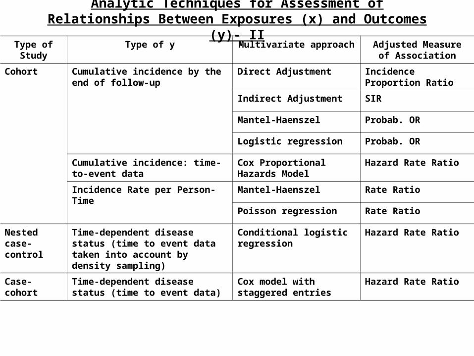
Analytic Techniques for Assessment of Relationships Between Exposures (x) and Outcomes (y)- II

Type of Study

Type of y Multivariate approach Adjusted Measure of Association

Cohort Cumulative incidence by the end of follow-up

Direct Adjustment Incidence Proportion Ratio

Indirect Adjustment SIR

Mantel-Haenszel Probab. OR

Logistic regression Probab. OR

Cumulative incidence: time-to-event data

Cox Proportional Hazards Model

Hazard Rate Ratio

Incidence Rate per Person-Time Mantel-Haenszel Rate Ratio

Poisson regression Rate Ratio

Nested case-control

Time-dependent disease status (time to event data taken into account by density sampling)

Conditional logistic regression

Hazard Rate Ratio

Case-cohort Time-dependent disease status (time to event data)

Cox model with staggered entries

Hazard Rate Ratio

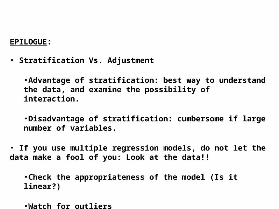
EPILOGUE:

• Stratification Vs. Adjustment

•Advantage of stratification: best way to understand the data, and examine the possibility of interaction.

•Disadvantage of stratification: cumbersome if large number of variables.

• If you use multiple regression models, do not let the data make a fool of you: Look at the data!!

•Check the appropriateness of the model (Is it linear?)

•Watch for outliers

• Consider the possibility of residual confounding.

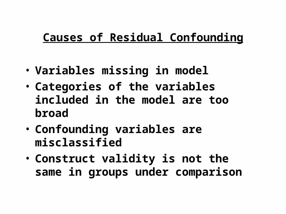
Causes of Residual Confounding

• Variables missing in model• Categories of the variables included in the

model are too broad• Confounding variables are misclassified• Construct validity is not the same in

groups under comparison

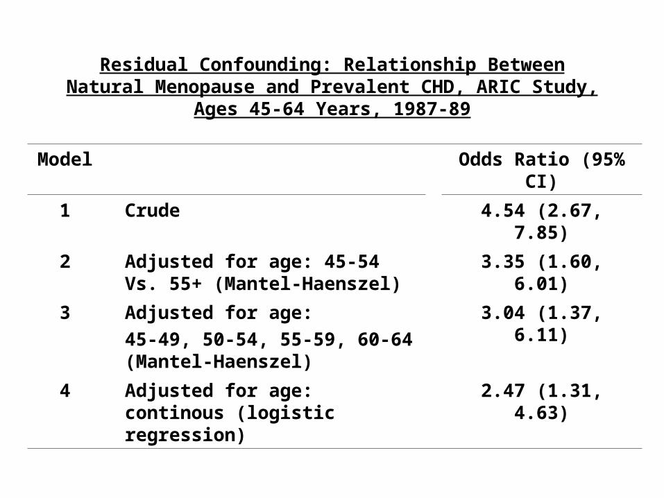
Residual Confounding: Relationship Between Natural Menopause and Prevalent CHD, ARIC Study, Ages 45-64

Years, 1987-89

Model Odds Ratio (95% CI)

1 Crude 4.54 (2.67, 7.85)

2 Adjusted for age: 45-54 Vs. 55+ (Mantel-Haenszel)

3.35 (1.60, 6.01)

3 Adjusted for age:

45-49, 50-54, 55-59, 60-64 (Mantel-Haenszel)

3.04 (1.37, 6.11)

4 Adjusted for age: continous (logistic regression)

2.47 (1.31, 4.63)

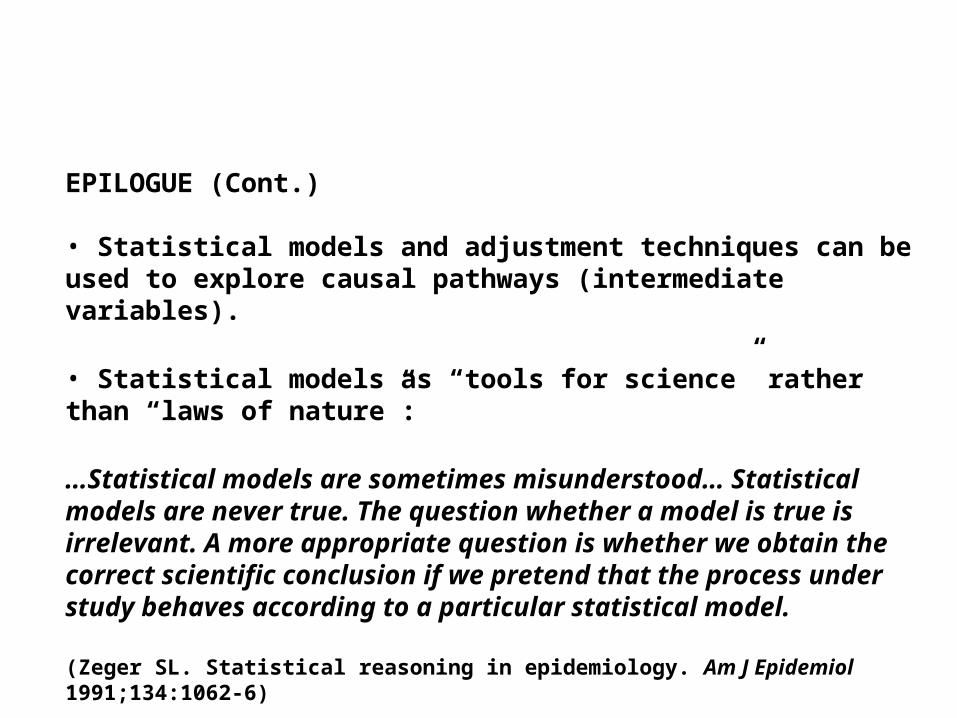
EPILOGUE (Cont.)

• Statistical models and adjustment techniques can be used to explore causal pathways (intermediate variables).

• Statistical models as “tools for science” rather than “laws of nature”:

…Statistical models are sometimes misunderstood… Statistical models are never true. The question whether a model is true is irrelevant. A more appropriate question is whether we obtain the correct scientific conclusion if we pretend that the process under study behaves according to a particular statistical model.

(Zeger SL. Statistical reasoning in epidemiology. Am J Epidemiol 1991;134:1062-6)