Multiple Climate States of Habitable Exoplanets:The Role of Obliquity and Irradiance

C. Kilic1,2,3, C. C. Raible1,2,3, and T. F. Stocker1,2,3,41 Climate and Environmental Physics, Physics Institute, University of Bern, Switzerland; stocker@climate.unibe.ch

2 Centre for Space and Habitability, University of Bern, Switzerland3 Oeschger Centre for Climate Change Research, University of Bern, Switzerland

Received 2017 April 3; revised 2017 May 29; accepted 2017 June 14; published 2017 August 1

Abstract

Stable, steady climate states on an Earth-size planet with no continents are determined as a function of the tilt of theplanet’s rotation axis (obliquity) and stellar irradiance. Using a general circulation model of the atmospherecoupled to a slab ocean and a thermodynamic sea ice model, two states, the Aquaplanet and the Cryoplanet, arefound for high and low stellar irradiance, respectively. In addition, four stable states with seasonally andperennially open water are discovered if comprehensively exploring a parameter space of obliquity from 0° to 90°and stellar irradiance from 70% to 135% of the present-day solar constant. Within 11% of today’s solar irradiance,we find a rich structure of stable states that extends the area of habitability considerably. For the same set ofparameters, different stable states result if simulations are initialized from an aquaplanet or a cryoplanet state. Thisdemonstrates the possibility of multiple equilibria, hysteresis, and potentially rapid climate change in response tosmall changes in the orbital parameters. The dynamics of the atmosphere of an aquaplanet or a cryoplanet state isinvestigated for similar values of obliquity and stellar irradiance. The atmospheric circulation substantially differsin the two states owing to the relative strength of the primary drivers of the meridional transport of heat andmomentum. At 90° obliquity and present-day solar constant, the atmospheric dynamics of an Aquaplanet state andone with an equatorial ice cover is analyzed.

Key words: planets and satellites: dynamical evolution and stability – planets and satellites: oceans – planets andsatellites: physical evolution – planets and satellites: terrestrial planets

1. Introduction

Habitability on exoplanets for known forms of life depends onthe presence of liquid water. This puts severe constraints on theclimatic conditions that result from the orbital configuration ofthe exoplanet, in particular stellar irradiation, the orientation of theplanet, rotation rates, atmospheric composition, and surfacealbedo, all of which are drivers of planetary surface temperature(Pierrehumbert 2010). Some of the largest climate variations on aplanetary surface are generated by the obliquity or tilt of theplanet’s rotation axis, that is, its orientation relative to the orbitaround the star. For instance, on Earth, obliquity is responsible notonly for the seasonal cycle but also for one of the strongest climatevariations, manifested as glacial–interglacial cycles with anamplitude of 3°C–4°C in global mean surface temperature overthe past 5million years (Masson-Delmotte et al. 2013). Changesin obliquity of the Earth during this time have a periodicity of41,000 years (Berger & Loutre 1991). Although they occur in anarrow range of 22°–24. 5 during the past 10million years, theyact as an effective pacemaker of substantial variations of theterrestrial ice mass and hence global sea level. This is evidenced inreconstructions of global sea level based on marine sediments(Huybers 2007; Lisiecki & Raymo 2007) and on the temperaturereconstructed from an Antarctic ice core (Jouzel et al. 2007).While in these records the obliquity cycle persisted throughout thepast 5 million years, in the past 800,000 years a longer cycle of

100,000 years, coinciding with the periodic variations of theeccentricity of the Earth’s orbit cycle, has become the dominantone. The importance of planetary obliquity has also beenrecognized for the habitability of exoplanets. Armstrong et al.(2014) have shown that oscillations in obliquity, caused by thegravitational interaction with nearby planets, can expand thehabitable zone of a planet considerably.Planetary mean surface temperature and the atmospheric

composition are fundamental quantities determining habitableconditions on a planetary surface. Surface temperature isdetermined by the net energy flux from the star reaching theplanet’s surface, which primarily depends on the stellarirradiance, the planetary albedo, and the composition of theatmosphere (H2O, CO2, CH4). Through Planck’s law, evensmall changes in stellar irradiance may cause fundamentalclimatic changes on a planet. Likewise, small changes ingreenhouse gas content of the atmosphere will producesubstantial climate changes through positive feedback effectssuch as the water vapor and ice–albedo feedbacks(Pierrehumbert 2010).The purpose of this paper is to comprehensively explore the

impact of changes in obliquity and in the stellar constant on theequilibrium climate of a planet in order to characterize possibleclimate states and determine their physical conditions, includ-ing habitability. Our study is therefore not limited to conditionsthat may have existed on Earth, but more generally itcontributes to the current and challenging research on thehabitability of exoplanets.The key determinant of planetary climate is the stellar

constant S; in the case of the Earth under current conditions,S 13610 = Wm−2. The first energy balance models demon-strated that reductions in S will cause transitions in the climatic

The Astrophysical Journal, 844:147 (13pp), 2017 August 1 https://doi.org/10.3847/1538-4357/aa7a03© 2017. The American Astronomical Society. All rights reserved.

4 Physics Institute, University of Bern, Sidlerstrasse 5 3012 Bern, Switzerland.

Original content from this work may be used under the termsof the Creative Commons Attribution 3.0 licence. Any further

distribution of this work must maintain attribution to the author(s) and the titleof the work, journal citation and DOI.

1

state from a habitable planet to a completely frozen planet(Budyko 1969; Sellers 1969). This is due to the temperature-dependent ice–albedo feedback, which is able to generatemultiple equilibrium states of the planet. This phenomenon wasfirst found in simple energy balance models (Budyko 1969;Sellers 1969; North et al. 1981) and is also simulated in state-of-the-art dynamical climate models (Rose & Marshall 2009;Ferreira et al. 2011; Linsenmeier et al. 2015). The occurrenceof different climate states is therefore independent of modelcomplexity. This insight has been offered as a physicalexplanation for geological indications of temporarily very coldconditions on Earth, in particular low-latitude glaciation some700 million years ago, referred to as the Snowball Earthhypothesis (Hoffmann & Schrag 2002). An alternative, butstill controversial, explanation is that the Earth may haveresided in a high-obliquity state caused by a giant impact at theearly stages of Earth with a subsequent rapid transition tocurrent low obliquity values some 500 million years ago(Williams 2008).

Qualitatively different instabilities can also occur atmoderately increased values of stellar irradiation, where arunaway greenhouse effect can be triggered. Using a one-dimensional model, Kasting (1988) found the occurrence ofrunaway at an irradiation of S1.4 0· for cloud-free conditionsand S4.8 0· for full cloud cover. A much lower threshold of

S1.4 0· for full cloud cover was reported by Popp et al. (2015).Recent simulations using comprehensive atmospheric modelsshow stable, moist greenhouse states (e.g., Popp et al. 2016) orconditions conducive to a runaway at about S1.2 0· (Wolf &Toon 2015). The threshold for a runaway greenhouse continuesto be debated (Goldblatt et al. 2013; Leconte et al. 2013).Taken together, even using comprehensive atmosphericmodels, it does not appear settled that a moderate increase ofirradiation, such as by 40%, necessarily results in a runawaygreenhouse.

The second determinant of planetary climate is theorientation of the rotation axis of a planet relative to its orbit.It governs the amount of energy that a planet receives from thestar at a given latitude in the course of a planet’s orbit aroundthe star. It is therefore responsible for both planetary meridionaltemperature gradients and seasonality. For small angles ofobliquity, the maximum input of annual mean energy is at theequator, while at the poles, the irradiance is strongly reduced.Because of these spatial differences, the atmosphere and oceanmust transport energy from the equator to the poles by meansof the general circulation (Lorenz 1967). The latitudinalgradient of annual mean energy supply to the planet changessign at an obliquity of about 54°: at higher values of obliquitymore energy is delivered to the polar latitudes than to thetropics (Jenkins 2000). In this situation, the atmosphere andocean will transport energy in the equatorward to achieve asteady state. With such fundamental changes of the spatialpattern of planetary energy supply, large climate changes on aplanet are expected if the obliquity changes.

Additionally, seasonality depends on obliquity ε. At zero tiltof the rotation axis, there are almost uniform conditionsthroughout the year, while at ε= 90° the amplitude of theseasonal cycle is at a maximum, with each latitude receiving noenergy from the star during some period of the year. Obliquityis highly variable among planets, as is evident in our solarsystem, where they range from ε= 0.01° for Mercury to 97.86°for Uranus, and 177.4° for Venus. Unfortunately, the tilt of

rotating exoplanets is not among the information that iscurrently available from astronomical observations (Winn &Fabrycky 2015), which leaves a key determinant of habitabilityunknown. With the recent discovery of entire planetary systemswithin the habitable zone (Gillon et al. 2017), such informationwould be particularly informative, and some research hasshown that this is in principle possible (Carter & Winn 2010;Zhu et al. 2014).Going beyond earlier studies that used highly simplified

energy balance models to illustrate possible climate states ofexoplanets (Spiegel et al. 2009), three-dimensional atmosphericmodels (Shields et al. 2013, 2014), and even comprehensiveclimate models for a small number of parameter values, such asstellar irradiation or obliquities (Ferreira et al. 2014; Hu &Yang 2014), here we employ a computationally efficientclimate model of intermediate complexity, the Planet Simulator(PlaSim) developed by Lunkeit et al. (2011). This allows us tocarry out extensive parameter exploration and a robust searchfor stable states. The model consists of a coarsely resolvedgeneral circulation model for the atmosphere coupled to a slabocean and a thermodynamic sea ice model. This modelrepresents the relevant dynamical processes of the atmosphericmeridional heat transport in a realistic manner and allowsseasonal or perennial sea ice cover if sea surface temperaturesfall below the freezing point. Here we use the model inaquaplanet configuration, that is, without any terrestrial surface.In a previous study with this model at lower resolution, theeffect of gradual changes of the solar constant at ε= 0°, 60°,and 90° was investigated (Linsenmeier et al. 2015). Theirresults suggest the existence of several climate states, but it isdifficult to establish whether these are true steady statesbecause the model was integrated for only 50 years.A more complex global model with a dynamical ocean

component in aquaplanet configuration was used by Ferreiraet al. (2014), who considered the cases of ε= 54° and 90° andpresent-day insolation. Only two equilibrium climates werefound: an Aquaplanet and a Snowball Earth, and theyconcluded that a stable state with equatorial ice was unlikely.Also, Earth configurations with modern and past continentaloutlines were used to assess the effect of high obliquity(Williams & Pollard 2003). They found a significant increase insnow accumulation during the winter for extreme seasonalvariations. However, this has not lead to a net annualaccumulation and subsequent glaciation, or even a transitionto a Snowball Earth.Today little is known about habitable conditions on Earth-

like exoplanets if the full range of obliquity is considered. It istherefore timely to explore in a comprehensive manner theentire parameter space of obliquity and stellar irradiance inorder to characterize the different steady-state climates thatspecific astronomical conditions are able to support. Our modelpermits a more realistic investigation of the meridionaltransport of heat carried by the atmospheric circulation in aspecific climate state. A further question that will be addressedhere concerns the circulation changes in an exoplanetatmosphere that result from transitions from one state toanother due to slowly changing astronomical parameters, thatis, state changes in the presence of multiple equilibria. Thisimplies hysteresis behavior and hence evolution-dependentclimatic conditions on an exoplanet.The paper is organized as follows. Section 2 describes the

climate model and the experimental setup. In Section 3 we

2

The Astrophysical Journal, 844:147 (13pp), 2017 August 1 Kilic, Raible, & Stocker

explore the parameter space and describe the various steady-state climates that are found. Section 4 presents transientexperiments and an analysis of the general circulation of theatmosphere with a focus on the differences between aCryoplanet and an Aquaplanet under nearly identical astro-nomical conditions. The special case of 90° obliquity isconsidered in Section 5, and discussions and conclusions arepresented in Section 6.

2. Climate Model and Experiments

In this study, the Planet Simulator, PlaSim, is used (Lunkeitet al. 2011). It is a climate model of intermediate complexityconsisting of a general circulation model for the atmosphere(AGCM) coupled to a slab ocean and a thermodynamic sea icemodel. The spectral resolution of the AGCM is T42,corresponding to a grid resolution of approximately 2.8°, and10 vertical levels are chosen. The radiation formulationresolves clear and cloudy sky for both long- and shortwaveradiation (Stephens 1978; Stephens et al. 1984), and thepresence of clouds and their effect on radiation are parameter-ized (Slingo & Slingo 1991). The model is run under Earth-likeconditions (planetary mass and radius, atmospheric composi-tion, rotation rate about the planetary axis, and form of theecliptic). Surface pressure is 1.01 10 Pa5· , and the concentra-tion of CO2 is kept constant at 360 ppm. The dynamicalatmosphere is coupled to a slab ocean in which heat istransported diffusively and which, through its heat capacity,serves as the slow component of the coupled climate system. Atthe ocean–atmosphere interface, sea ice can be formed if thesea surface temperature falls below the freezing point. Thisgenerates a positive feedback to perturbations through changesof the albedo. The albedo of open ocean surface is 0.069,whereas the albedo of the sea ice surface is temperaturedependent with a maximum value of 0.7 (Lunkeit et al. 2011).The minimum snow albedo is 0.4 for 0°C surface temperatureand increases linearly up to 0.8 for surface temperatures smallerthan −10°C. The model represents a compromise betweencomplexity, permitting the analysis of atmospheric circulationand planetary surface changes, and efficiency, allowingcomprehensive exploration of the parameter space, hereobliquity and stellar constant.

Our model has reduced complexity in several aspects. It usesclassical, simplified cloud parameterizations, and the sea icemodel is thermodynamic. With a slab ocean of 50 m depth,ocean heat transport is represented as a diffusive flux. Hence,potential effects of changing ocean circulation cannot becaptured with our model. Although this could have importantconsequences for the meridional distribution of heat and thepresence of multiple equilibria, recent simulations suggest thatthe overall effect of ocean dynamics is limited and that a slabocean is a good approximation for the major feedbackprocesses involving the storage and distribution of heat bythe ocean (Ferreira et al. 2014).

To focus on the fundamental physical processes, we select anaquaplanet configuration for all simulations (Kilic et al. 2017).Three different types of sensitivity simulations are performedwhile changing the two parameters obliquity and stellarconstant: (1) simulations starting from a warm initial climatestate (Aquaplanet), (2) simulations starting from a cold initialclimate state (Cryoplanet), and (3) transient simulationscontinuously changing one of the two parameters and keepingthe other constant. The first two types of simulations are

performed for different combinations of parameters and runinto an equilibrium state. Obliquity varies from 0°, in which noseasonal variations are present, to 90°, where the planet’srotation axis lies in the orbital plane. For irradiance, we chose arange of S S S0= ˜ · with S 1361 W m0

2= - , and S̃ varies from0.7 to 1.35. Simulations were integrated for 100 years, bywhich time a steady state was diagnosed based on the globalmean surface temperature and global mean sea ice thickness.For the “warm start” setup, 367 simulations were performed,for the “cold start” 200. The third setup consists of fourtransient simulations where the obliquity is fixed and the stellarconstant is continuously increased from S 0.52=˜ to 1.27 forε= 47°, and S 0.87=˜ to 1.35 for ε= 23.44° with a rate ofchange in stellar constant of 0.01% per year. Using the sameobliquities, the stellar constant is decreased starting fromS 1.27=˜ and S 1.3=˜ , respectively, for the other twosimulations. We note that in the range of S̃ considered here,all simulations are run to steady state. Therefore, the presenceof a runaway greenhouse can be excluded in our modelsimulations. For example, the maximum values of annual meansurface temperature and surface humidity are about 65°C and149 g kg−1, respectively, for S 1.35=˜ and ε= 15°. This ischaracteristic of a moist greenhouse (Kasting 1988).

3. A Diversity of Stable Climate States Depending onObliquity and Irradiation

Here we present the first systematic exploration of parameterspace of the two determinants of planetary climate, stellarirradiance and obliquity. We find several qualitatively differentsteady states and identify areas in parameter space where,depending on the initial conditions, two stable states exist(Figure 1). In total we have identified six stable climate states,as summarized in Table 1. These states are classified into twogeneral types: Aquaplanets with a dominant water surface, andCryoplanets with a predominantly frozen surface. These twotypes are well known from previous studies using a hierarchyof models. In fact, the first latitude-dependent energy balancemodels have already simulated these two stable states(Budyko 1969; Sellers 1969), and many later modeling studieshave confirmed their existence.Depending on the specific values of obliquity and irradiance,

several variants of these two types emerge (Table 1). This isrelevant because it significantly enlarges the area of habitabilityin this parameter space, here defined as the presence of waterduring some period of the year. It is evident that irrespective ofobliquity a Cryoplanet occurs for low stellar irradiances, whilean Aquaplanet is simulated for high values of irradiance. Thesimulations show that the exact location where either of thesetwo types prevails depends on the initial conditions. However,we find a rich structure of stable climate states for intermediatevalues of these two parameters (Figure 1).Starting from Earth-like conditions, with the relative stellar

irradiance S S S 10= =˜ and ε= 23.44°, and using a cryopla-net state as the initial condition, the planet remains completelyfrozen for these values of irradiance and obliquity (Figure 1(a)).If, on the other hand, the initial condition is an aquaplanet state,we find the Capped Aquaplanet (Figure 1(b)). This state has apermanent ice cover in the polar areas with an ice edge positionthat varies seasonally (Figure 2). The model therefore exhibitstwo stable states for the same parameter values at this locationin parameter space. This is indicated by the overlaid stateboundaries of Figure 1(b) in Figure 1(a).

3

The Astrophysical Journal, 844:147 (13pp), 2017 August 1 Kilic, Raible, & Stocker

If obliquity or irradiance are slightly increased, the permanentice cover in the polar areas becomes seasonal because of the

increased energy supply to the high latitudes. This state is termedNear Aquaplanet. It occurs in a very narrow region in parameterspace (Figure 1(b)) and can only be reached from aquaplanet initialconditions. If obliquity is further increased, the polar ice coverdisappears completely, resulting in a permanent ocean surface, oran Aquaplanet. The Aquaplanet is a state that occupies a widerange in parameter space. In particular for S 1.04>˜ , it occurs forall obliquities (Figure 1(b)) if simulations are initialized from anAquaplanet, and for S 1.3>˜ if they are started from a Cryoplanet(Figure 1(a)). This is the consequence of multiple equilibria that wefind to be a robust feature of our simulations. The Aquaplanetsurvives down to about S 0.83=˜ , provided there is sufficientseasonal energy input, which is the case of ε= 60°.Starting again from Earth-like conditions in the Capped

Aquaplanet state, but now reducing stellar irradiance, a Cryoplanetresults, which is the steady state with a complete ice coverthroughout the year (Figure 2). For S 0.74<˜ this state occursindependent of obliquity. Increasing seasonality will supplysufficient energy to the high latitudes so that the ice cover opensseasonally if S 0.73>˜ . This state is called Near Cryoplanet. Itfeatures a band of ice extending from the tropics to the highlatitudes with an open polar ocean during the summer season(Figure 2).Finally, if starting a simulation from cryoplanet conditions with,

for example, S 1=˜ and ε= 90°, we find the UncappedCryoplanet, which is the sixth stable state (Figure 2). It consistsof a low-latitude ice cover and a perennial ocean at high latitudes.This state was also reported by Linsenmeier et al. (2015) andoccurred in the range of S0.95 1.05< <˜ in their model. Here weconfirm the existence of this sixth steady state in our modelconfiguration with increased grid resolution and longer integrationtime. The seasonal and latitudinal characteristics of the six states

Figure 1. Regions of six distinct stable climate states in obliquity–irradiance space determined from 567 simulations using a dynamical atmosphere–slab ocean–sea icemodel. The simulations used the parameter combinations indicated by gray dots and were started from cryoplanet (a) or aquaplanet conditions (b). Integrations werecarried out for 100 years to steady state. Boundaries of regions that are not supported by symbols are interpolated. Four of the six possible states (Table 1) can bereached by initiating the simulations from a cryoplanet (a), and five from an aquaplanet initial state (b). The state boundaries of panel (b) are reproduced as white lineson panel (a) in order to determine the possible presence of multiple equilibria. For example, for S 1=˜ and 90e = the Uncapped Cryoplanet coexists with theAquaplanet state. The area of habitability is on the right side of the state boundary of the Cryoplanet, and it differs in size depending on the initial conditions; that is,the evolution history of the exoplanet is crucial in determining the current climate. The white star indicates the location of current Earth conditions in parameter space.

Table 1Characteristics of Multiple Stable Climate States

Climate State SurfaceLatitudeExtent Seasonality

InitialCond.

Aquaplanet Ocean global perennial aq, crIce L L

Near Aquaplanet Ocean 60S–60N perennial aqOcean 60–90 seasonalIce 60–90 seasonal

Capped Aquaplanet Ocean 60S–60N perennial aqIce 60–90 perennial

Cryoplanet Ice global perennial aq, crOcean L L

Near Cryoplanet Ice 60S–60N perennial aq, crIce 60–90 seasonalOcean 60–90 seasonal

Uncapped Cryoplanet Ice 60S–60N perennial crOcean 60–90 perennial

Notes. Stable climate states are found for ranges in obliquity from 0° to 90° and instellar irradiance from 70% to 135% of today’s solar constant, and simulations arestarted from aquaplanet or cryoplanet initial conditions. The states can be classifiedin two types: Aquaplanets and Cryoplanets, with variants depending on thepresence of seasonal ice cover or ocean surface. The notion “perennial” does notsuggest an absence of a seasonal cycle but the presence of ice or ocean throughoutthe year. Sea surface temperature or ice thickness will still exhibit a seasonal cyclein these cases (see Figure 2).

4

The Astrophysical Journal, 844:147 (13pp), 2017 August 1 Kilic, Raible, & Stocker

are displayed in Figure 2 using Hovmöller diagrams. Thesymmetry of the two types of Cryoplanets and Aquaplanets andtheir respective stable variants should be noted: each state of onetype has its counterpart in the other type.

Our finding of the Uncapped Cryoplanet state is evidenceagainst the supposition of Ferreira et al. (2014) that a stablestate with an equatorial ice cover is unlikely to exist. It isinteresting to hypothesize why they did not find this state withtheir more comprehensive model that has a dynamical ocean.Orbital parameters were almost identical to those we use here.With ε= 90° and S 1=˜ and starting from an Aquaplanet, their

model remains in this stable state. The results using a slabocean component instead are very similar, leading them toconclude that the ocean is simply storing and releasing heat asin a one-dimensional column (Ferreira et al. 2014). Ourextensive sampling of the parameter space does not indicate thepresence of an Uncapped Cryoplanet if the simulations startfrom an aquaplanet. This is consistent with the finding ofFerreira et al. (2014). We find the Uncapped Cryoplanet stateonly if we start from a Cryoplanet, as is indicated in Figure 1,where the complete area of this state is shared by theaquaplanet state. We therefore speculate that the more complete

Figure 2. Latitude–time Hovmöller diagrams of latitude and month for illustrative examples of the six stable states in the parameter space of obliquity and relativestellar irradiance displayed in Figure 1. Contours are sea surface temperature (SST) and sea ice thickness. The states fall into two types that can be characterized asCryoplanet (left column) and Aquaplanet (right column). Each state has a counterpart in the other type. Habitable conditions—here defined as the presence of liquidwater during some time of the year—are found in all states but the Cryoplanet. The states are obtained by starting the simulation from aquaplanet or cryoplanetconditions. The location of these states in parameter space are indicated in Figure 3.

5

The Astrophysical Journal, 844:147 (13pp), 2017 August 1 Kilic, Raible, & Stocker

climate model of Ferreira et al. (2014) would also sustain astable equatorial ice cover for high obliquity if it had startedfrom cryoplanet conditions.

Note also that Figure 1 exhibits a certain degree of symmetry.The orientation of the boundary between Aquaplanet states andCryoplanet states in parameter space indicates a general trade-offbetween irradiance and seasonality. For higher seasonality, asmaller amount of total energy from the star is necessary for atransition from a Cryoplanet to an Aquaplanet. The location of this

transition depends on the initial climate state. For high values ofobliquity and low irradiance, a seasonal opening of the ice cover athigh latitudes is simulated. For low values of obliquity, a stable icecover in polar areas throughout the year can be sustained on anAquaplanet, generating the Capped Aquaplanet state.

4. Transition from an Aquaplanet to a Cryoplanet:Impact on Atmospheric Circulation

Multiple equilibria are a robust feature of our simulations. Theyare present in a large range of relative stellar irradiance for

S0.83 1.3< <˜ and for all obliquities, as evidenced by the whiteboundaries in Figure 1(a). This can also be seen in Figure 3,where the two panels of Figure 1 are laid on top of each other.Depending on the exact values of the two parameters, different

pairs of stable states are found. For example, under Earth-likeconditions of S 1=˜ and ε= 23.44°, we find both the Cryoplanetand the Capped Aquaplanet, while if we increase obliquities to90°, four more pairs of steady states are visited (Figure 3). Exceptfor the parameter values where the Cryoplanet is found as a singlesteady state, the entire space produces conditions that permit atleast the seasonal presence of water and hence are favorable forlife in some regions on the planet.Some of the stable states can be accessed only from specific

initial states. The Capped and Near Aquaplanets cannot bereached from a cryoplanet initial state, since for these parametervalues the Cryoplanet is the other stable equilibrium. TheUncapped Cryoplanet, on the other hand, can only be reachedwhen simulations start from a Cryoplanet. A completerealization of possible steady states therefore requires simula-tions starting from different initial states.We now present two examples of transient simulations

across state boundaries by slowly varying stellar irradiance

Figure 3. Hovmöller diagrams of the six steady states in the parameter space of obliquity and relative stellar irradiance. Five states are obtained by starting thesimulation from an Aquaplanet (solid pointer line), whereas the Uncapped Cryoplanet state only results from a start from a Cryoplanet (dashed pointer line). Theexample of S 1=˜ and ε = 90° illustrates one case of multiple equilibria for these parameter values resulting from the initial conditions of Aquaplanet and Cryoplanet,respectively. The distribution of steady states in parameter space is depicted as the combination of the two panels in Figure 1. The striped color patterns of the centerpanel indicate that two equilibrium states coexist for the same parameter values, according to the colors of the stripes. Hysteresis is possible in the striped area.

Figure 4. Hysteresis of planetary annual mean temperature for variations in thestellar constant of S t 10 yr4 1D D = - -˜ illustrated at ε = 47° (solid line) andε = 23.44° (dashed line).

6

The Astrophysical Journal, 844:147 (13pp), 2017 August 1 Kilic, Raible, & Stocker

(Figure 4). At ε= 47° there is a single state boundary that iscrossed between S 0.9=˜ and 0.89 (solid line). A smaller jumpin planetary annual mean temperature already occurs aroundS 1.06=˜ . For ε= 23.44°, the simulation successively crossesthree state boundaries (dashed line) if the simulations start fromthe aquaplanet, whereas only one boundary is crossed in thepath back along the lower branch of the hysteresis.

Across a state boundary, only small changes in theparameters suffice to generate large changes in all climatevariables, in particular the atmospheric circulation of an

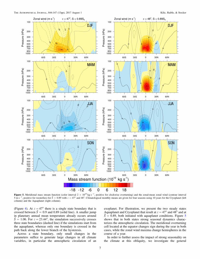
exoplanet. For illustration, we present the two steady statesAquaplanet and Cryoplanet that result at ε= 47° and 48° and atS 0.89=˜ , both initiated with aquaplanet conditions. Figure 5shows that in both states strong seasonal dynamics charac-terizes the atmospheric circulation. The meridional overturningcell located at the equator changes sign during the year in bothcases, while the zonal wind maxima change hemispheres in thecourse of a year.In order to further assess the impact of strong seasonality on

the climate at this obliquity, we investigate the general

Figure 5. Meridional mass stream function (color interval 2 × 1010 kg s−1, positive for clockwise overturning) and the zonal-mean zonal wind (contour interval5 m s−1, positive for westerlies) for S 0.89=˜ with ε = 47° and 48°. Climatological monthly means are given for four seasons using 10 years for the Cryoplanet (leftcolumn) and the Aquaplanet (right column).

7

The Astrophysical Journal, 844:147 (13pp), 2017 August 1 Kilic, Raible, & Stocker

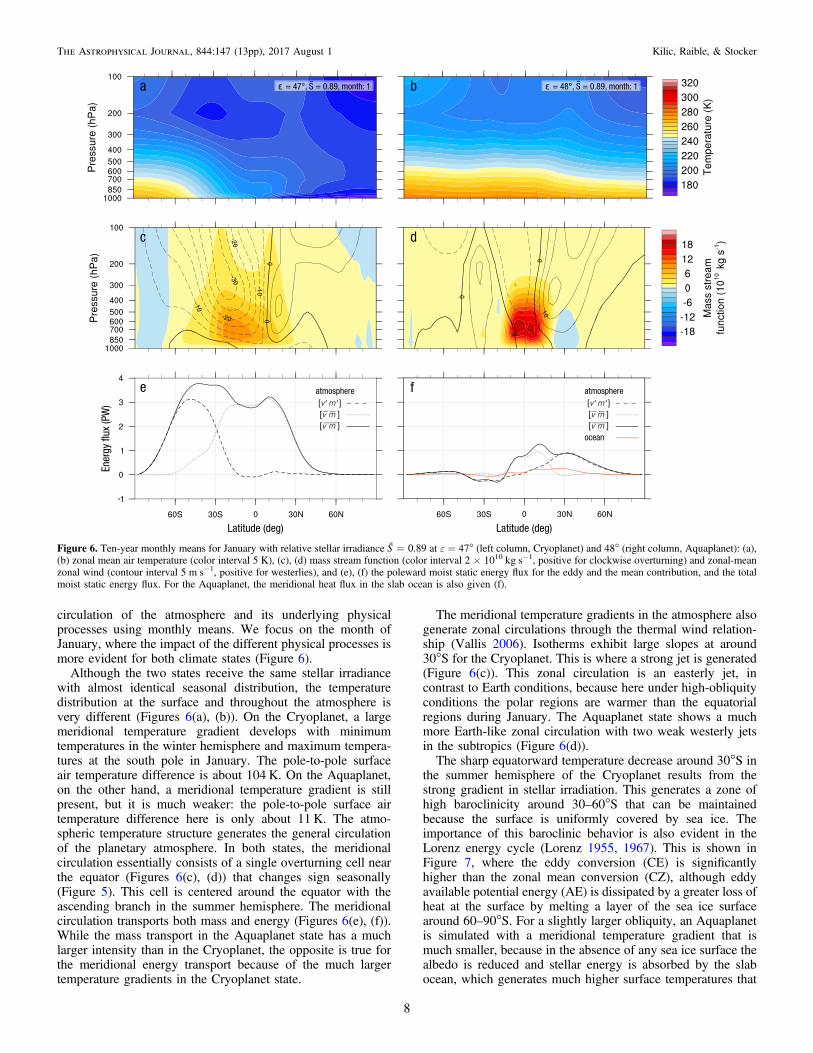
circulation of the atmosphere and its underlying physicalprocesses using monthly means. We focus on the month ofJanuary, where the impact of the different physical processes ismore evident for both climate states (Figure 6).

Although the two states receive the same stellar irradiancewith almost identical seasonal distribution, the temperaturedistribution at the surface and throughout the atmosphere isvery different (Figures 6(a), (b)). On the Cryoplanet, a largemeridional temperature gradient develops with minimumtemperatures in the winter hemisphere and maximum tempera-tures at the south pole in January. The pole-to-pole surfaceair temperature difference is about 104 K. On the Aquaplanet,on the other hand, a meridional temperature gradient is stillpresent, but it is much weaker: the pole-to-pole surface airtemperature difference here is only about 11 K. The atmo-spheric temperature structure generates the general circulationof the planetary atmosphere. In both states, the meridionalcirculation essentially consists of a single overturning cell nearthe equator (Figures 6(c), (d)) that changes sign seasonally(Figure 5). This cell is centered around the equator with theascending branch in the summer hemisphere. The meridionalcirculation transports both mass and energy (Figures 6(e), (f)).While the mass transport in the Aquaplanet state has a muchlarger intensity than in the Cryoplanet, the opposite is true forthe meridional energy transport because of the much largertemperature gradients in the Cryoplanet state.

The meridional temperature gradients in the atmosphere alsogenerate zonal circulations through the thermal wind relation-ship (Vallis 2006). Isotherms exhibit large slopes at around30°S for the Cryoplanet. This is where a strong jet is generated(Figure 6(c)). This zonal circulation is an easterly jet, incontrast to Earth conditions, because here under high-obliquityconditions the polar regions are warmer than the equatorialregions during January. The Aquaplanet state shows a muchmore Earth-like zonal circulation with two weak westerly jetsin the subtropics (Figure 6(d)).The sharp equatorward temperature decrease around 30°S in

the summer hemisphere of the Cryoplanet results from thestrong gradient in stellar irradiation. This generates a zone ofhigh baroclinicity around 30–60°S that can be maintainedbecause the surface is uniformly covered by sea ice. Theimportance of this baroclinic behavior is also evident in theLorenz energy cycle (Lorenz 1955, 1967). This is shown inFigure 7, where the eddy conversion (CE) is significantlyhigher than the zonal mean conversion (CZ), although eddyavailable potential energy (AE) is dissipated by a greater loss ofheat at the surface by melting a layer of the sea ice surfacearound 60–90°S. For a slightly larger obliquity, an Aquaplanetis simulated with a meridional temperature gradient that ismuch smaller, because in the absence of any sea ice surface thealbedo is reduced and stellar energy is absorbed by the slabocean, which generates much higher surface temperatures that

Figure 6. Ten-year monthly means for January with relative stellar irradiance S 0.89=˜ at ε = 47° (left column, Cryoplanet) and 48° (right column, Aquaplanet): (a),(b) zonal mean air temperature (color interval 5 K), (c), (d) mass stream function (color interval 2 × 1010 kg s−1, positive for clockwise overturning) and zonal-meanzonal wind (contour interval 5 m s−1, positive for westerlies), and (e), (f) the poleward moist static energy flux for the eddy and the mean contribution, and the totalmoist static energy flux. For the Aquaplanet, the meridional heat flux in the slab ocean is also given (f).

8

The Astrophysical Journal, 844:147 (13pp), 2017 August 1 Kilic, Raible, & Stocker

persist in the winter hemisphere. This leads to a significantlyless baroclinic atmosphere. Energy fluxes under such condi-tions are quantified in the Lorenz energy cycle (Figure 7),where all energy conversions are rather small compared to theCryoplanet state.

To further examine reasons for the different characteristics ofthe meridional circulation and the temperature pattern, weanalyze the meridional energy transport in the atmosphere bycalculating the moist static energy (MSE) flux v m =·v m v m+ ¢ ¢· · , where v is the meridional velocity and m isthe MSE given by m c T g z L qp e= + +· · · with c 1004p =J kg−1 K−1 the specific heat capacity of dry air, L 2.5 10e

6= ·J kg−1 the latent heat of vaporization, T the temperature, z theheight, and q the specific humidity. The overbars and primesdenote the time mean and its deviation, so the two terms on theright-hand side of the equation quantify the transport by themean flow and by the transient eddies.

The MSE flux around the equator is dominated by thetransport of the mean flow for both states (Figures 6(e), (f)). ThisMSE flux is related to thermally direct cells (Figures 6(c), (d)).However, the driving mechanisms are different in the two states:under cryoplanet conditions, only radiative heating around theequator is able to drive the thermally direct cell. Latent heating isalmost absent because there is no open water. For the aquaplanetstate, both radiative and latent heating are the main drivers of thisthermally direct cell (Figure 8). They are both stronger due to thepresence of a warm ocean surface that acts as a source of heatand moisture.

The part of the MSE flux (Figures 6(e), (f)) related to eddiesbehaves differently for the two states. The Cryoplanet shows a

peak contribution of eddy flux around 50°S, which overlapswith parts of a thermally direct cell (Figure 6(c)). This is incontrast to the Aquaplanet state, where we find a peakcontribution around 30°N, which coincides with a thermallyindirect cell (Figure 6(d)).To assess this difference, we consider the zonal mean pattern

of meridional eddy heat and momentum fluxes (Figure 9). Forthe cryoplanet state, the maximum eddy heat flux occurs in thelower troposphere at about 55–60°S (Figure 9(a)) withconvergence of eddy heat flux north and divergence south ofthis maximum. Therefore, the eddy heat transport is northwardand tends to reduce the pole-to-equator mean temperaturegradient. Furthermore, the gradient of eddy momentum flux inthe range 35–65°S is negative (Figure 9(c)) and thus illustratesa convergence of the eddy momentum flux. This convergencedecreases with height for the lower troposphere up to 500 hPa,which implies a clockwise circulation (Figure 9(c)). Thus, athermally indirect meridional cell in the southern hemisphere(Figure 6(c)) results, which turns clockwise as the thermaldirect cell between 30°S and 30°N. For the Aquaplanet, themaximum eddy heat flux is at about 30–40°N (Figure 9(b)),leading again to a northward heat transport. The gradient of themomentum flux (Figure 9(d)) is negative, showing thatmomentum flux converges, and this convergence increaseswith height in the lower troposphere up to 400 hPa around30°–40°, resulting in a counterclockwise, thermally indirectmean meridional cell.In summary, the main difference between the two states is

that the dominant meridional circulation cell is a thermallydirect cell, driven by radiative and latent heating under

Figure 7. Lorenz energy cycle for S 0.89=˜ with ε = 47° (Cryoplanet) and 48° (Aquaplanet) based on climatological monthly means for January using 10 years.Arrows indicate the direction of energy conversions (unit: Wm−2), and circles represent energy reservoirs (unit:105 Jm−2). The area of the energy reservoir circles andthe width of the conversion bars scale with their values.

9

The Astrophysical Journal, 844:147 (13pp), 2017 August 1 Kilic, Raible, & Stocker

aquaplanet conditions (similar to Earth), whereas the dominantcell of the cryoplanet state is driven by a combination ofradiative heating and eddy heat and momentum fluxes, and thusis a superposition of a thermally direct and a thermallyindirect cell.

5. Two Stable States at 90° Obliquity

The stable state that features a permanent ice cover fromabout 30°S to 30°N and a permanent open ocean toward thepoles was identified for S 1=˜ and ε= 90°. The UncappedCryoplanet occurs only when simulations are started from acryoplanet state (Figures 1 and 3). This state does not occur as asingle equilibrium but is always paired with the aquaplanetstate. Figure 10 compares these two stable states at ε= 90° forthe month of January. Although stellar radiation is identical, thestrong ice–albedo feedback causes very cold temperaturesabove the equatorial ice cover. The presence of the ocean as anefficient heat storage maintains warm temperatures at highlatitudes even when the stellar irradiation is zero during thewinter season (Figure 10(a)). One overturning cell is located atthe ice edge in the summer hemisphere and supports asubsidence at the equator that may stabilize the ice cover

(Figure 10(c)). The strong meridional temperature gradientsthroughout the atmospheric column at 30°S generate a strongeasterly jet. Note that the meridional ocean heat flux under theice cover vanishes (Figure 10(e)).At the same parameter values, the Aquaplanet exhibits very

warm surface temperatures at all latitudes (Figure 10(b)), withocean heat storage maintaining ice-free conditions during thewinter season. In the summer hemisphere, large meridionaltemperature gradients develop a strong easterly jet and a strongmeridional overturning circulation, which is the primarymechanism for heat transport convergence (Figure 10(d)).The structures of the zonal wind and the circulation cell areremarkably similar in the two states, although the Aquaplanet’smeridional circulation is much stronger. This is driven by thelatent heat release over the open ocean surface, as was alreadyseen in Figure 8(d). Related to the different strengths of thecirculation and jets, an important deviation between the twostates is illustrated in the meridional energy flux, as for latitudessouth of 30°S the transient part dominates for the UncappedCryoplanet state due to increased baroclinicity (increasedtemperature gradient). This is in contrast to the aquaplanetstate, where the mean circulation part of the energy flux drivesa poleward flux between 30 and 50°S.

Figure 8. (a), (b) Diabatic and (c), (d) latent heating rate (color interval 10 2- J kg−1 s−1) for S 0.89=˜ with ε = 47° (Cryoplanet, left column), and 48° (Aquaplanet,right column), based on climatological monthly means for January using 10 years.

10

The Astrophysical Journal, 844:147 (13pp), 2017 August 1 Kilic, Raible, & Stocker

6. Discussion and Conclusions

Stellar irradiance and obliquity are key determinants of thesurface climate conditions of a planet. We have demonstratedthat a richer variety of stable states can be simulated by acoupled atmosphere–slab ocean–sea ice climate model than justthe two classical types of an Aquaplanet and a Cryoplanet withperennial open water and sea ice surface, respectively. Eachtype comes in three variants with specific surface character-istics in the high latitudes. High obliquity causes a strongenergy input in the high latitudes during the summer. Byincreasing the stellar irradiance of a Cryoplanet at highobliquity, the polar ice cap is melted during the summer,resulting in a Near Cryoplanet state. Further increasing thestellar irradiances then generates an Uncapped Cryoplanet withan open polar ocean throughout the year. Finally, upon evenstronger irradiance, the ice is completely melted and anAquaplanet results. Similarly, if starting from an Aquaplanet atstrong irradiance and low obliquity, a reduction of irradianceproduces first a Near Aquaplanet with seasonal polar ice coverand then a Capped Aquaplanet with a perennial polar sea ice,before transiting to a Cryoplanet. Hence a quite symmetricdistribution of stable states results, which suggests that thereare many more possibilities for habitability on an exoplanet

than hitherto assumed on the basis of commonly used energybalance models.We have also presented an examination of the atmospheric

circulation and the meridional heat transport for the twoextreme states of the Aquaplanet and the Cryoplanet. Thepresence of multiple equilibria is a robust feature of oursimulations. It owes its existence to the ice–albedo feedback,which has been first described using zonally averaged energybalance models. As a consequence, hysteresis behavior exists,which implies that the current climate on an exoplanet dependson the evolution of a planet’s orbital configuration, in particularthe evolution of irradiance, or distance from the star, as well asof obliquity. The zone of habitability in the irradiance–obliquity parameter space is more extended if the planetevolves from an aquaplanet than from a cryoplanet.Our study has some limitations that are primarily associated

with the type of climate model that we have employed. Adynamical ocean component, including a dynamic sea icemodel, would be an obvious extension. Such a slowlyresponding component could generate a more complex solutionstructure by permitting different circulation modes in the ocean,which would modify the transport of heat meridionally. Thechemical composition of the atmosphere, in particular theconcentrations of greenhouse gases, would also strongly

Figure 9. (a), (b) Eddy heat (color interval 2 K m s−1) and (c), (d) momentum flux (color interval 2 m2 s−2) for S 0.89=˜ with ε = 47° (Cryoplanet, left column) and48° (Aquaplanet, right column), based on climatological monthly means for January using 10 years.

11

The Astrophysical Journal, 844:147 (13pp), 2017 August 1 Kilic, Raible, & Stocker

influence the results. By modifying the outgoing longwaveradiation due to changed greenhouse gas concentrations,changes in annual mean energy fluxes in addition to theseasonal variations by obliquity would occur that would havean impact on the occurrence and characteristics of the steadystates.

In summary, we have demonstrated that the tilt of theplanet’s rotation axis with respect to the orbit is a crucialparameter in determining habitability under multiple equilibria.While astronomical observations of exoplanetary systems,combined with model simulations, provide reliable estimatesof stellar irradiance, the geometry of the planets’ orbit, and theirmasses, some fundamental orbital information to determinehabitability on an exoplanet is still elusive. Future efforts ofastronomical observation should be directed to determine theobliquity of a planet in order to better assess the conditions ofpotential habitability on an exoplanet.

Continuous model support by E. Kirk and F. Lunkeit isacknowledged. Simulations were carried out at UBELIX of theUniversity of Bern and at the Swiss National SupercomputingCenter (CSCS). We acknowledge constructive comments by ananonymous reviewer. This work has been funded by the Centerfor Space and Habitability of the University of Bern. C.C.R.received support from the Oeschger Center for Climate Change

Research, and T.F.S. was supported by the Swiss NationalScience Foundation.

References

Armstrong, J. C., Barnes, R., Domagal-Goldman, S., et al. 2014, AsBio,14, 277

Berger, A., & Loutre, M. F. 1991, QSRv, 10, 297Budyko, M. I. 1969, Tell, 21, 611Carter, J. A., & Winn, J. N. 2010, ApJ, 716, 850Ferreira, D., Marshall, J., O’Gorman, P. A., & Seager, S. 2014, Icar, 243, 236Ferreira, D., Marshall, J., & Rose, B. 2011, JCli, 24, 992Gillon, M., Triaud, A. H. M. J., Demory, B.-O., et al. 2017, Natur, 542, 456Goldblatt, C., Robinson, T. D., Zahnle, K. J., & Crisp, D. 2013, NatGe, 6, 661Hoffmann, P. F., & Schrag, D. P. 2002, TeNov, 14, 129Hu, Y. Y., & Yang, J. 2014, PNAS, 111, 629Huybers, P. 2007, QSRv, 26, 37Jenkins, G. S. 2000, JGR, 105, 7357Jouzel, J., Masson-Delmotte, V., Cattani, O., et al. 2007, Sci, 317, 793Kasting, J. F. 1988, Icar, 74, 472Kilic, C., Raible, C. C., Stocker, T. F., & Kirk, E. 2017, P&SS, 135, 1Leconte, J., Forget, F., Charnay, B., Wordsworth, R., & Pottier, A. 2013,

Natur, 504, 268Linsenmeier, M., Pascale, S., & Lucarini, V. 2015, P&SS, 105, 43Lisiecki, L. E., & Raymo, M. E. 2007, QSRv, 26, 56Lorenz, E. N. 1955, Tell, 7, 157Lorenz, E. N. 1967, The Nature and Theory of the General Circulation of the

Atmosphere (Geneva: World Meteorological Organization), 161Lunkeit, F., Borth, H., Böttinger, M., et al. 2011, Planet Simulator—Reference

Manual Version 16, Meteorological Institute (Univ. Hamburg)

Figure 10. Ten-year monthly means for January with relative stellar irradiance S 1=˜ at ε = 90° for the Uncapped Cryoplanet (left column) and the Aquaplanet (rightcolumn): (a), (b) zonal mean air temperature (color interval 5 K), (c), (d) mass stream function (color interval 2 × 1010 kg s−1, positive for clockwise overturning) andzonal-mean zonal wind (contour interval 5 m s−1, positive for westerlies), and (e), (f) the poleward moist static energy flux for the eddy and the mean contribution, thetotal moist static energy flux, and the meridional heat flux in the slab ocean. Note the different scale of the y axis in panels (e) and (f) compared to Figure 6.

12

The Astrophysical Journal, 844:147 (13pp), 2017 August 1 Kilic, Raible, & Stocker

Masson-Delmotte, V., Schulz, M., Abe-Ouchi, A., et al. 2013, in ClimateChange 2013: The Physical Science Basis. Contribution of Working GroupI to the Fifth Assessment Report of the Intergovernmental Panel on ClimateChange, ed. T. F. Stocker et al. (Cambridge: Cambridge Univ. Press), 383

North, G. R., Cahalan, R. F., & Coakley, J. A. 1981, RvGSP, 19, 91Pierrehumbert, R. T. 2010, Principles of Planetary Climate (Cambridge:

Cambridge Univ. Press), 647Popp, M., Schmidt, H., & Marotzke, J. 2015, JAtS, 72, 452Popp, M., Schmidt, H., & Marotzke, J. 2016, NatCo, 7, 10627Rose, B. E., & Marshall, J. 2009, JAtS, 66, 2828Sellers, W. D. 1969, JApMe, 8, 392Shields, A. L., Bitz, C. M., Meadows, V. S., Joshi, M. M., & Robinson, T. D.

2014, ApJL, 785, L9

Shields, A. L., Meadows, V. S., Bitz, C. M., Pierrehumbert, R. T.,Joshi, M. M., & Robinson, T. D. 2013, AsBio, 13, 715

Slingo, A., & Slingo, J. M. 1991, JGR, 96, 15341Spiegel, D. S., Menou, K., & Schaft, C. A. 2009, ApJ, 691, 596Stephens, G. L. 1978, JAtS, 35, 2123Stephens, G. L., Ackerman, S., & Smith, E. A. 1984, JAtS, 41, 687Vallis, G. K. 2006, Atomspheric and Oceanic Fluid Dynamics (Cambridge:

Cambridge Univ. Press)Williams, D. M., & Pollard, D. 2003, IJAsB, 2, 1Williams, G. E. 2008, ESRv, 87, 61Winn, J. N., & Fabrycky, D. C. 2015, ARA&A, 53, 409Wolf, E. T., & Toon, O. B. 2015, JGR, 120, 5775Zhu, W., Huang, C. X., Zhou, G., & Lin, D. N. C. 2014, ApJ, 796, 1

13

The Astrophysical Journal, 844:147 (13pp), 2017 August 1 Kilic, Raible, & Stocker