multiphase ﬂows examples solved with ansys cfx

Ing. Paola RanutProf. Enrico NobileUniversità degli Studi di TriesteDipartimento di Ingegneria e Architettura

Corso di Termofluidodinamica Computazionale

Multiphase flows

Examples solved with ANSYS CFX

A.A. 2013-2014

CONTENTS 1

Contents

1 Example: particle tracking 31.1 Definition of the Reynolds number for the backward-facing step problem . . . 41.2 Available data . . . . . . . . . . . . . . . . . . . . . . . . . . . . . . . . . . . 41.3 CFD simulation . . . . . . . . . . . . . . . . . . . . . . . . . . . . . . . . . . 51.4 Set up of the CFD simulation . . . . . . . . . . . . . . . . . . . . . . . . . . . 6

1.4.1 Expressions . . . . . . . . . . . . . . . . . . . . . . . . . . . . . . . . 61.4.2 Definition of a new material . . . . . . . . . . . . . . . . . . . . . . . 61.4.3 Default domain settings . . . . . . . . . . . . . . . . . . . . . . . . . 61.4.4 Boundary conditions: inlet . . . . . . . . . . . . . . . . . . . . . . . . 81.4.5 Other Boundary conditions . . . . . . . . . . . . . . . . . . . . . . . . 81.4.6 Output Control . . . . . . . . . . . . . . . . . . . . . . . . . . . . . . 81.4.7 Solver Control . . . . . . . . . . . . . . . . . . . . . . . . . . . . . . 9

1.5 Results . . . . . . . . . . . . . . . . . . . . . . . . . . . . . . . . . . . . . . . 101.6 Comments . . . . . . . . . . . . . . . . . . . . . . . . . . . . . . . . . . . . . 16

1.6.1 Effect of the number of particles . . . . . . . . . . . . . . . . . . . . . 161.6.2 Effect of buoyancy . . . . . . . . . . . . . . . . . . . . . . . . . . . . 161.6.3 Velocity profile from expression . . . . . . . . . . . . . . . . . . . . . 161.6.4 Velocity profile from file . . . . . . . . . . . . . . . . . . . . . . . . . 19

1.7 Suggested exercises . . . . . . . . . . . . . . . . . . . . . . . . . . . . . . . . 19

2 Example: collapse of a water column (dam breaking problem) 212.1 Computational mesh . . . . . . . . . . . . . . . . . . . . . . . . . . . . . . . 212.2 Set up of the CFD computation . . . . . . . . . . . . . . . . . . . . . . . . . . 21

2.2.1 Expressions . . . . . . . . . . . . . . . . . . . . . . . . . . . . . . . . 222.2.2 Analysis Type . . . . . . . . . . . . . . . . . . . . . . . . . . . . . . . 232.2.3 Domain: Default Domain . . . . . . . . . . . . . . . . . . . . . . . . 242.2.4 Boundary conditions . . . . . . . . . . . . . . . . . . . . . . . . . . . 262.2.5 Solver control . . . . . . . . . . . . . . . . . . . . . . . . . . . . . . . 272.2.6 Output Control . . . . . . . . . . . . . . . . . . . . . . . . . . . . . . 27

2.3 Numerical results . . . . . . . . . . . . . . . . . . . . . . . . . . . . . . . . . 28

P. Ranut, E. Nobile - Aprile 2014

1 Example: particle tracking 3

1 Example: particle tracking

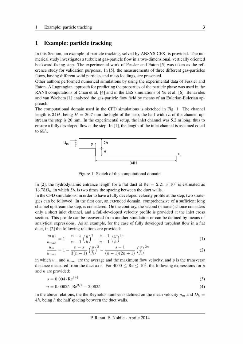
In this Section, an example of particle tracking, solved by ANSYS CFX, is provided. The nu-merical study investigates a turbulent gas-particle flow in a two-dimensional, vertically orientedbackward-facing step. The experimental work of Fessler and Eaton [5] was taken as the ref-erence study for validation purposes. In [5], the measurements of three different gas-particlesflows, having different solid particles and mass loadings, are presented.Other authors performed numerical simulations by using the experimental data of Fessler andEaton. A Lagrangian approach for predicting the properties of the particle phase was used in theRANS computations of Chan et al. [4] and in the LES simulations of Yu et al. [6]. Benavidesand van Wachem [1] analyzed the gas-particle flow field by means of an Eulerian-Eulerian ap-proach.The computational domain used in the CFD simulations is sketched in Fig. 1. The channellength is 34H , being H = 26.7 mm the hight of the step; the half-width h of the channel up-stream the step is 20 mm. In the experimental setup, the inlet channel was 5.2 m long, thus toensure a fully developed flow at the step. In [1], the length of the inlet channel is assumed equalto 65h.

2h

H

y

x

34H

Uin

Figure 1: Sketch of the computational domain.

In [2], the hydrodynamic entrance length for a flat duct at Re = 2.21 × 105 is estimated as13.75Dh, in which Dh is two times the spacing between the duct walls.In the CFD simulations, in order to have a fully developed velocity profile at the step, two strate-gies can be followed. In the first one, an extended domain, comprehensive of a sufficient longchannel upstream the step, is considered. On the contrary, the second (smarter) choice considersonly a short inlet channel, and a full-developed velocity profile is provided at the inlet crosssection. This profile can be recovered from another simulation or can be defined by means ofanalytical expressions. As an example, for the case of fully developed turbulent flow in a flatduct, in [2] the following relations are provided:

u(y)umax

= 1− n− sn− 1

(yh

)2− s− 1n− 1

(yh

)2n(1)

um

umax= 1− n− s

3(n− 1)

(yh

)2− s− 1

(n− 1)(2n+ 1)

(yh

)2n(2)

in which um and umax are the average and the maximum flow velocity, and y is the transversedistance measured from the duct axis. For 4000 ≤ Re ≤ 105, the following expressions for sand n are provided:

s = 0.004 ·Re3/4 (3)

n = 0.00625 ·Re3/4 − 2.0625 (4)

In the above relations, the the Reynolds number is defined on the mean velocity um and Dh =4h, being h the half spacing between the duct walls.


4 1.1 Definition of the Reynolds number for the backward-facing step problem

1.1 Definition of the Reynolds number for the backward-facing step problem

The literature offers several definitions of the characteristic length for a backward-facing stepproblem, which lead to different definitions of the Reynolds number, as stressed in [3]. Withreference with the variables reported in Fig. 1, the Reynolds number can be defined as:

ReDh =ρUb4hµ

(5a)

Re2h =ρUb2hµ

(5b)

ReH =ρUbH

µ(5c)

in which Ub is the average velocity of the inlet flow.Fessler and Eaton [5] provide two other definitions, one for flow in the inlet channel:

Reh =ρU0h

µ(6)

and the other for the flow downwards the step:

ReH =ρU0H

µ(7)

in which U0 is the centerline velocity of the inlet flow.

1.2 Available data

The experimental data reported in [5] are summarized in Tab. 1 and Tab. 2.

Nominal diameter (µm) 90 150 70Material glass glass copperDensity (kg ·m−3) 2500 2500 8800Stokes mean particle time constant, τpStokes (ms) 61 167 130Modified mean particle time constant, τp (ms) 38 92 88Large-eddy Stokes number, St 3.0 7.2 6.9Particle Reynolds number, Rep 7.3 11.8 5.5Mass loading 20% 20%, 40% 3%, 10%

Table 1: Particle parameters.

Centreline velocity, U0 (ms−1) 10.5Channel flow, Reh 13800Backward-facing step flow, ReH 1840090 µm glass velocity (ms−1) 0.46150 µm glass velocity (ms−1) 0.9270 µm copper velocity (ms−1) 0.88

Table 2: Fluid parameters.

As the reader certainly knows, the Stokes number St quantifies the nature of the kinetic equi-librium between the particles and the surrounding fluid. For St � 1 the particulate phase does


1.3 CFD simulation 5

not affect the motion of the fluid phase, and a one-way coupling approach can be applied. Viceverse, for St � 1 the inertia effect of particles becomes significant, and a two-way couplingtechnique must be used.The Stokes number is defined as the ratio of the particle response time τp to a representativetime scale in the flow τf :

St =τpτf

(8)

In the case of a creeping flow1 of solid spherical particles in a gaseous medium, the effect of thefluid density can be neglected and the particle response time can be expressed as:

τpStokes =ρpd

2p

18µ(9)

where ρp is the particle density, dp is the particle diameter and µ is the dynamic viscosity of thefluid. However, in the case of no-creeping flows, an alternative definition of τp must be used; in[5], the following modified time constant is employed:

τp =τpStokes

1 + Re0.687p

(10)

being Rep the Reynolds number characterizing the particle motion, defined as:

Rep =dpUrel

ν(11)

In the above equation, Urel is a velocity scale which characterizes the average slip velocity ofparticle relative to the flow.In [5], the fluid time scale was defined as:

τf =5HU0

(12)

1.3 CFD simulation

Benavides and van Wachem [1] employed a 65h channel upwards the step, corresponding to alength of 2.6 m. In order to obtain a center-line velocity U0 of about 10.5 m/s at the step (x/H =0), they imposed a uniform velocity Uin = 9.3 m/s at the inlet of the channel, corresponding toa Reynolds number of 1.3 × 104. Chan et al. [4] specified, at the inlet of the backward facingstep flow, the profiles of velocity previously computed on a 5.2 m long channel flow.For the particle phase, at the inlet Chan et al. [4] specified, in the streamwise direction, thevelocities recovered during the experiment and reported in Tab. 2 (0.88 m/s for the 70µm copperparticles), while the transverse velocity components were set to zero. However, Benavides andvan Wachem [1] claim that inlet velocity of the particulate phase does not influence the results.In the present simulation, two different solution strategies are followed. In the first one, anextended geometry is considered, comprehensive of a 3 m inlet channel. The length of thechannel was chosen in order to have a fully developed velocity profile at the outlet, and isintermediate between the lengths of [1] and [4]. However, as the post processing confirmed, aslightly shorter inlet channel could have been used.

1A creeping flow, also named Stokes flow, is a type of fluid flow in which the inertial forces are small comparedwith the viscous forces. These flows are characterized by Re � 1.


6 1.4 Set up of the CFD simulation

In the second approach, the inlet channel is omitted, and only the fluid domain from x/H = 0is considered. The profiles of velocity for the gas and particle phase are initialized with the datacomputed on a flat duct of height 2h and length 3 m. Here after, this flat duct will be indicatedas initialization duct.In order to get Reh and ReH as close as to the values reported in [5], both in the extendeddomain and in the initialization duct, a uniform streamwise velocity of 9.77 m/s was specifiedat the inlet. The resulting Reynolds numbers are Reh = 13796 and ReH = 18417, while thecenterline velocity at x/H = 0 is U0 = 10.66 m/s. On the contrary, in order to have a centerlinevelocity U0 = 10.5 m/s, as that reported in [5], a free stream velocity of 9.62 m/s should beapplied, which provides Reh = 13587 and ReH = 18139. However, the differences betweenthe two cases are negligible and, therefore, in the next sections only the results computed withan inlet velocity of 9.77 m/s will be illustrated.

1.4 Set up of the CFD simulation

1.4.1 Expressions

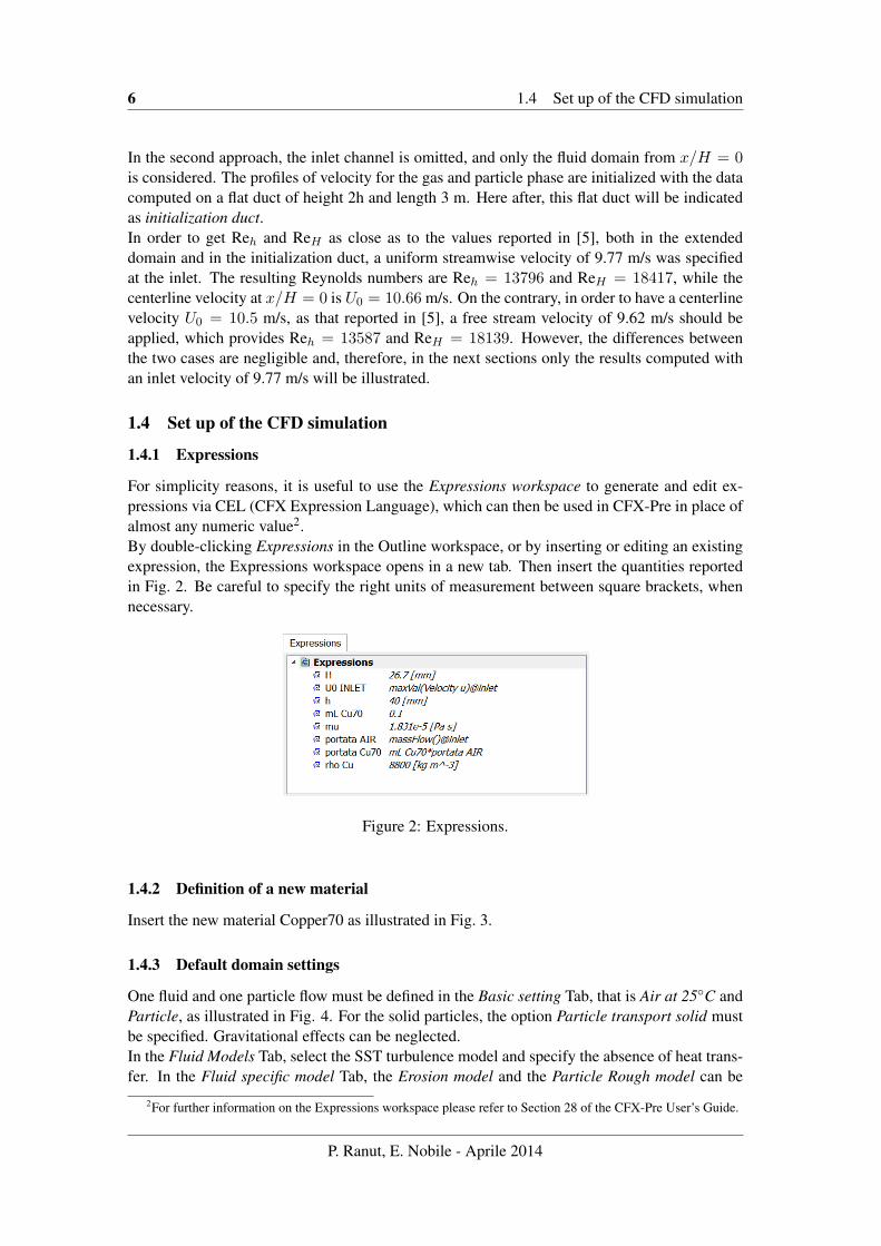
For simplicity reasons, it is useful to use the Expressions workspace to generate and edit ex-pressions via CEL (CFX Expression Language), which can then be used in CFX-Pre in place ofalmost any numeric value2.By double-clicking Expressions in the Outline workspace, or by inserting or editing an existingexpression, the Expressions workspace opens in a new tab. Then insert the quantities reportedin Fig. 2. Be careful to specify the right units of measurement between square brackets, whennecessary.

Figure 2: Expressions.

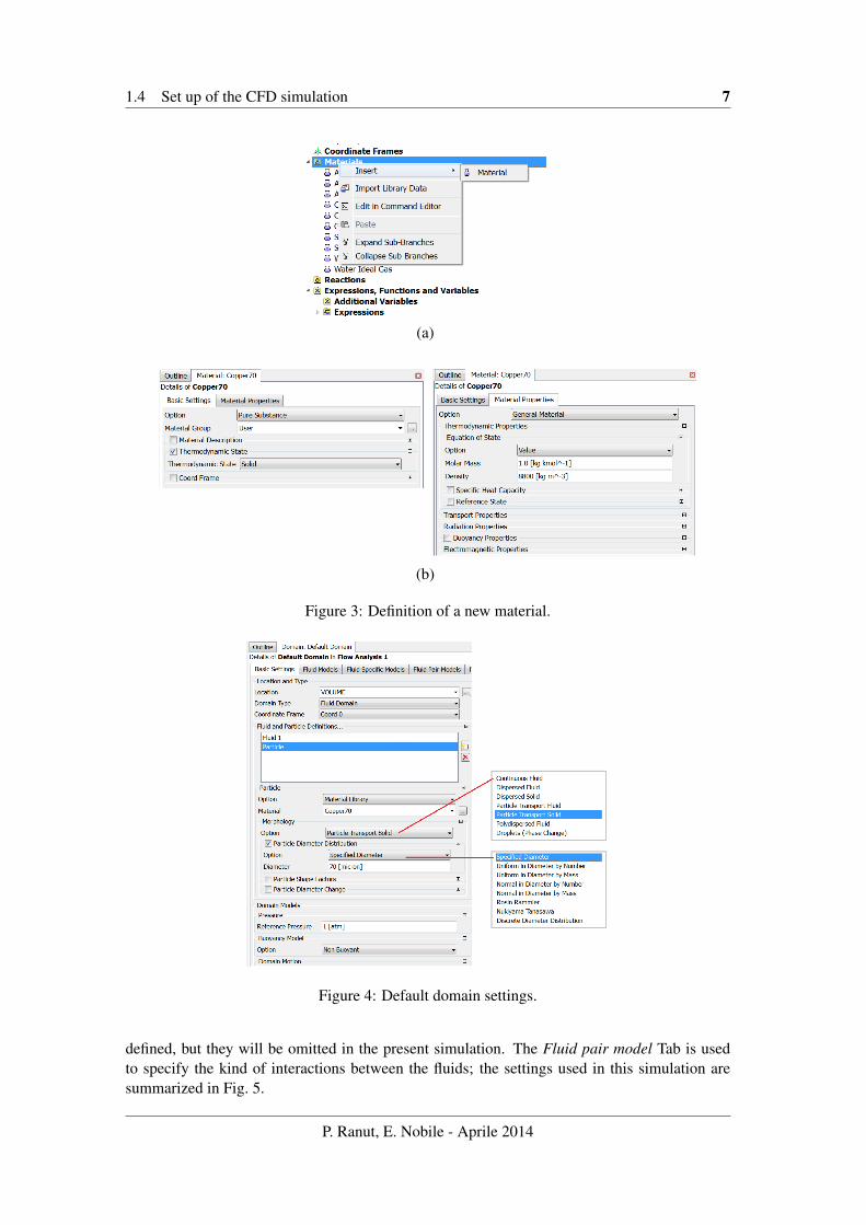
1.4.2 Definition of a new material

Insert the new material Copper70 as illustrated in Fig. 3.

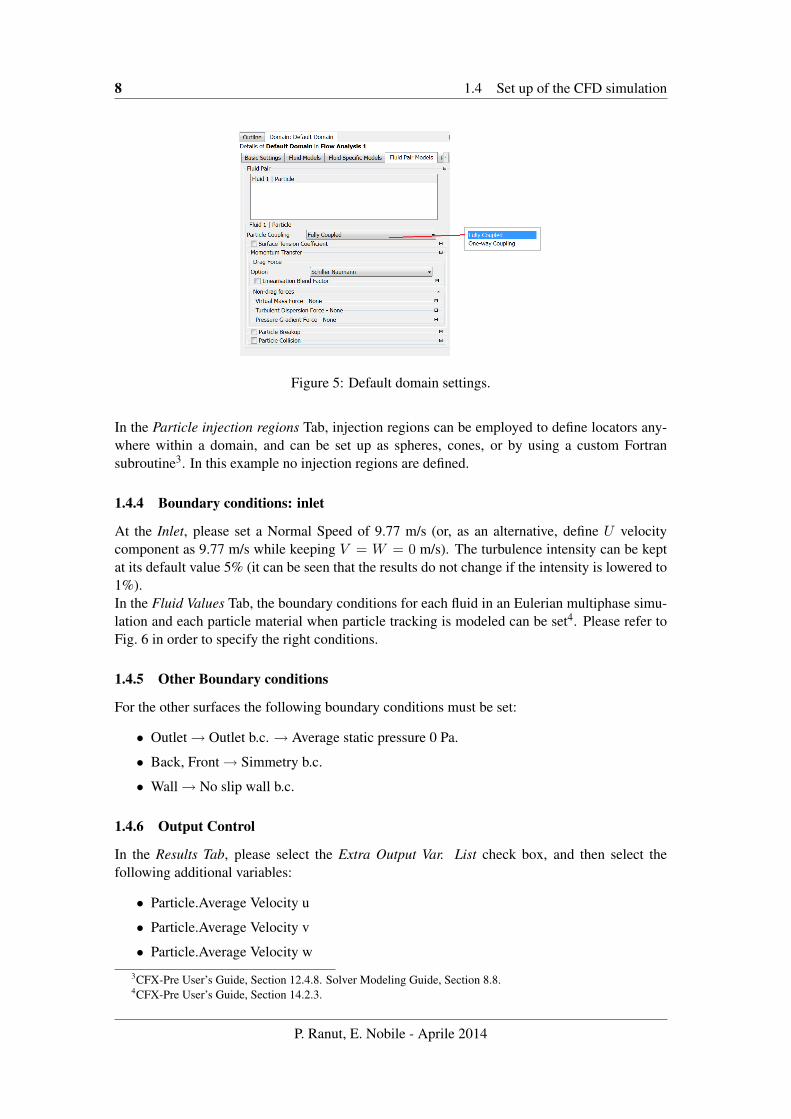
1.4.3 Default domain settings

One fluid and one particle flow must be defined in the Basic setting Tab, that is Air at 25◦C andParticle, as illustrated in Fig. 4. For the solid particles, the option Particle transport solid mustbe specified. Gravitational effects can be neglected.In the Fluid Models Tab, select the SST turbulence model and specify the absence of heat trans-fer. In the Fluid specific model Tab, the Erosion model and the Particle Rough model can be

2For further information on the Expressions workspace please refer to Section 28 of the CFX-Pre User’s Guide.


1.4 Set up of the CFD simulation 7

(a)

(b)

Figure 3: Definition of a new material.

Figure 4: Default domain settings.

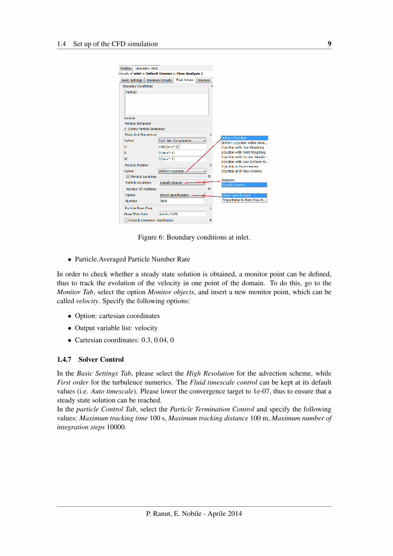
defined, but they will be omitted in the present simulation. The Fluid pair model Tab is usedto specify the kind of interactions between the fluids; the settings used in this simulation aresummarized in Fig. 5.


8 1.4 Set up of the CFD simulation

Figure 5: Default domain settings.

In the Particle injection regions Tab, injection regions can be employed to define locators any-where within a domain, and can be set up as spheres, cones, or by using a custom Fortransubroutine3. In this example no injection regions are defined.

1.4.4 Boundary conditions: inlet

At the Inlet, please set a Normal Speed of 9.77 m/s (or, as an alternative, define U velocitycomponent as 9.77 m/s while keeping V = W = 0 m/s). The turbulence intensity can be keptat its default value 5% (it can be seen that the results do not change if the intensity is lowered to1%).In the Fluid Values Tab, the boundary conditions for each fluid in an Eulerian multiphase simu-lation and each particle material when particle tracking is modeled can be set4. Please refer toFig. 6 in order to specify the right conditions.

1.4.5 Other Boundary conditions

For the other surfaces the following boundary conditions must be set:

• Outlet→ Outlet b.c. → Average static pressure 0 Pa.

• Back, Front→ Simmetry b.c.

• Wall→ No slip wall b.c.

1.4.6 Output Control

In the Results Tab, please select the Extra Output Var. List check box, and then select thefollowing additional variables:

• Particle.Average Velocity u

• Particle.Average Velocity v

• Particle.Average Velocity w

3CFX-Pre User’s Guide, Section 12.4.8. Solver Modeling Guide, Section 8.8.4CFX-Pre User’s Guide, Section 14.2.3.


1.4 Set up of the CFD simulation 9

Figure 6: Boundary conditions at inlet.

• Particle.Averaged Particle Number Rate

In order to check whether a steady state solution is obtained, a monitor point can be defined,thus to track the evolution of the velocity in one point of the domain. To do this, go to theMonitor Tab, select the option Monitor objects, and insert a new monitor point, which can becalled velocity. Specify the following options:

• Option: cartesian coordinates

• Output variable list: velocity

• Cartesian coordinates: 0.3, 0.04, 0

1.4.7 Solver Control

In the Basic Settings Tab, please select the High Resolution for the advection scheme, whileFirst order for the turbulence numerics. The Fluid timescale control can be kept at its defaultvalues (i.e. Auto timescale). Please lower the convergence target to 1e-07, thus to ensure that asteady state solution can be reached.In the particle Control Tab, select the Particle Termination Control and specify the followingvalues: Maximum tracking time 100 s, Maximum tracking distance 100 m, Maximum number ofintegration steps 10000.


10 1.5 Results

1.5 Results

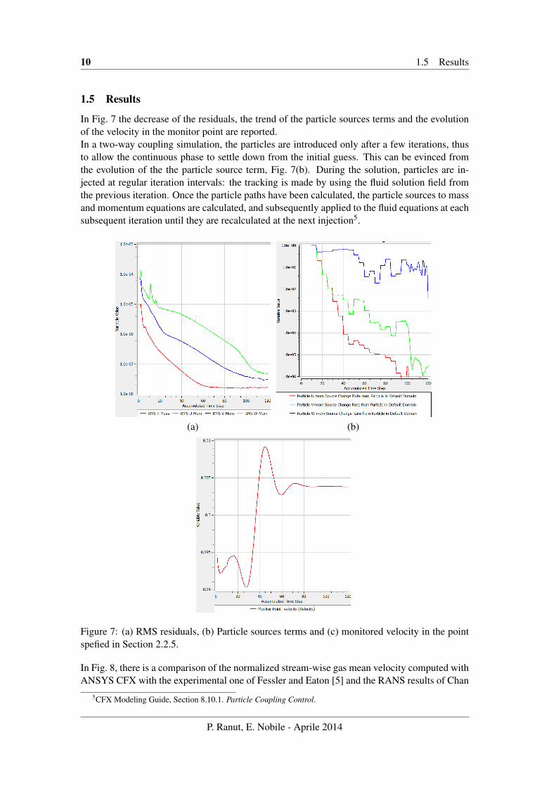
In Fig. 7 the decrease of the residuals, the trend of the particle sources terms and the evolutionof the velocity in the monitor point are reported.In a two-way coupling simulation, the particles are introduced only after a few iterations, thusto allow the continuous phase to settle down from the initial guess. This can be evinced fromthe evolution of the the particle source term, Fig. 7(b). During the solution, particles are in-jected at regular iteration intervals: the tracking is made by using the fluid solution field fromthe previous iteration. Once the particle paths have been calculated, the particle sources to massand momentum equations are calculated, and subsequently applied to the fluid equations at eachsubsequent iteration until they are recalculated at the next injection5.

(a) (b)

Figure 7: (a) RMS residuals, (b) Particle sources terms and (c) monitored velocity in the pointspefied in Section 2.2.5.

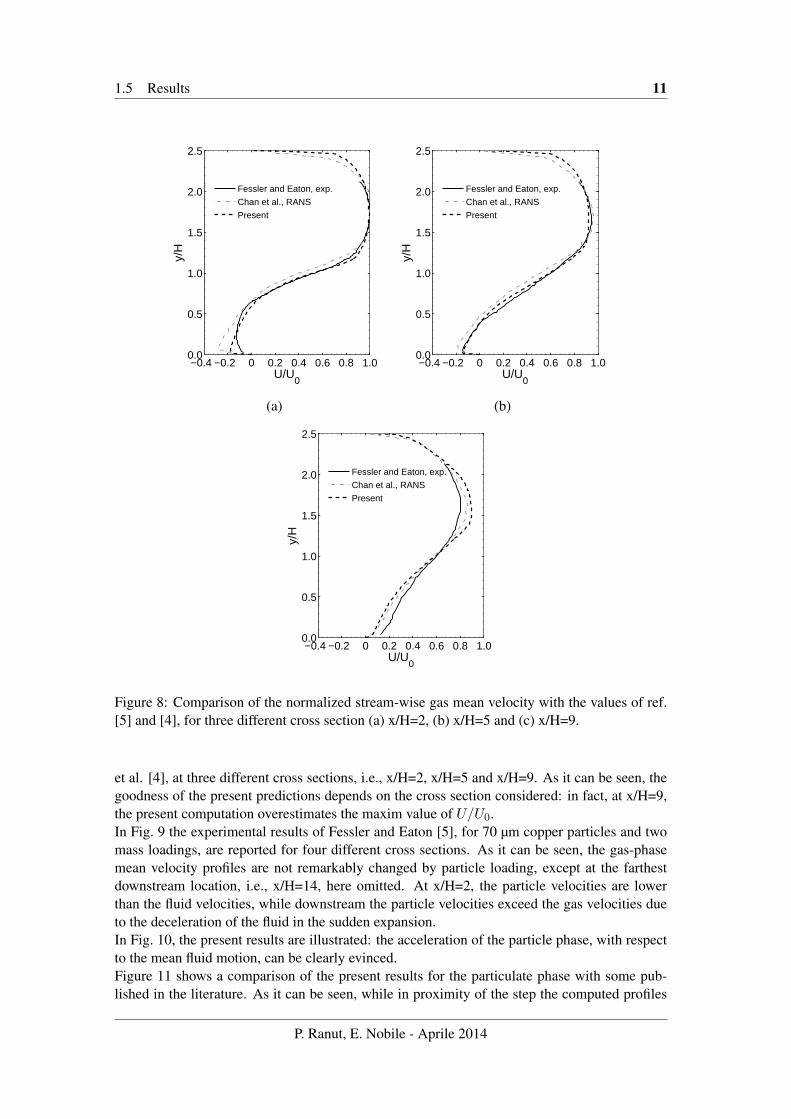
In Fig. 8, there is a comparison of the normalized stream-wise gas mean velocity computed withANSYS CFX with the experimental one of Fessler and Eaton [5] and the RANS results of Chan

5CFX Modeling Guide, Section 8.10.1. Particle Coupling Control.


1.5 Results 11

−0.4 −0.2 0 0.2 0.4 0.6 0.8 1.00.0

0.5

1.0

1.5

2.0

2.5

U/U0

y/H

Fessler and Eaton, exp.

Chan et al., RANS

Present

(a)

−0.4 −0.2 0 0.2 0.4 0.6 0.8 1.00.0

0.5

1.0

1.5

2.0

2.5

U/U0

y/H


Chan et al., RANS

Present

(b)

−0.4 −0.2 0 0.2 0.4 0.6 0.8 1.00.0

0.5

1.0

1.5

2.0

2.5

U/U0

y/H


Chan et al., RANS

Present

Figure 8: Comparison of the normalized stream-wise gas mean velocity with the values of ref.[5] and [4], for three different cross section (a) x/H=2, (b) x/H=5 and (c) x/H=9.

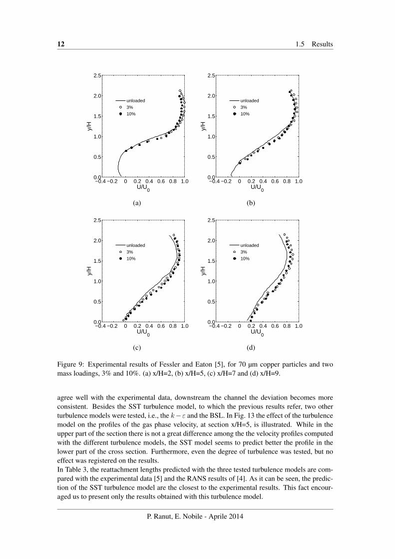
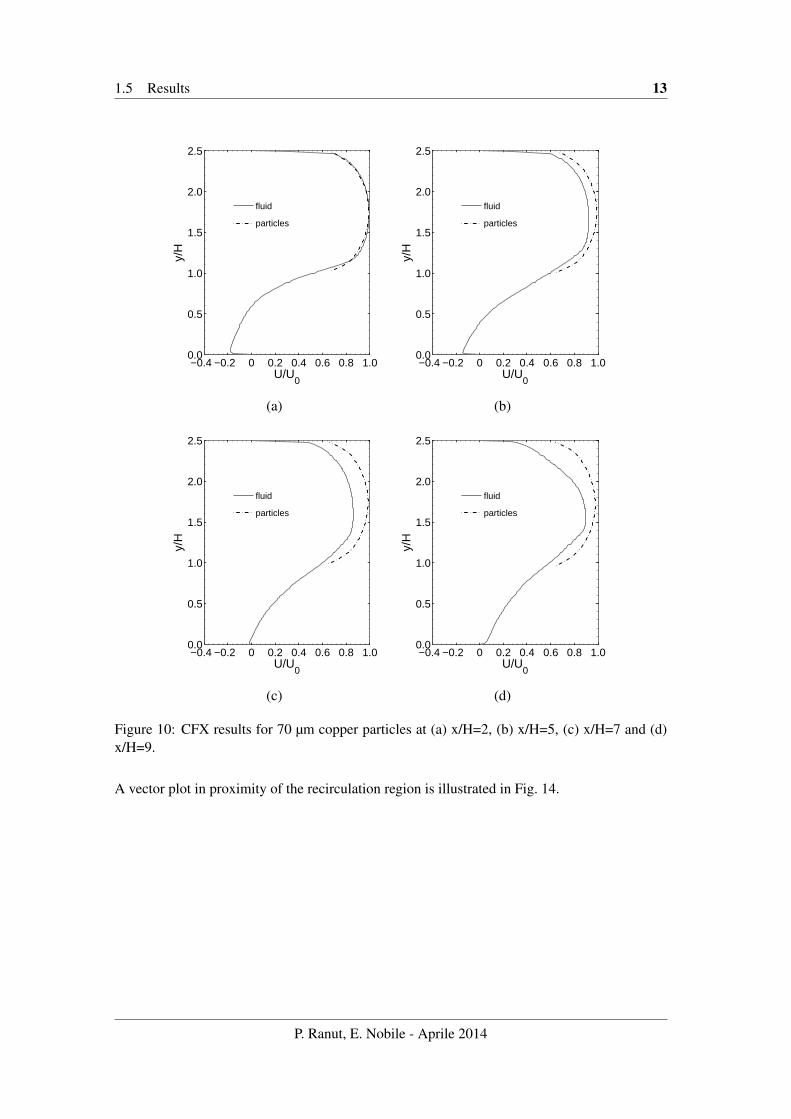
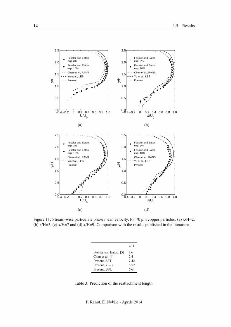
et al. [4], at three different cross sections, i.e., x/H=2, x/H=5 and x/H=9. As it can be seen, thegoodness of the present predictions depends on the cross section considered: in fact, at x/H=9,the present computation overestimates the maxim value of U/U0.In Fig. 9 the experimental results of Fessler and Eaton [5], for 70 µm copper particles and twomass loadings, are reported for four different cross sections. As it can be seen, the gas-phasemean velocity profiles are not remarkably changed by particle loading, except at the farthestdownstream location, i.e., x/H=14, here omitted. At x/H=2, the particle velocities are lowerthan the fluid velocities, while downstream the particle velocities exceed the gas velocities dueto the deceleration of the fluid in the sudden expansion.In Fig. 10, the present results are illustrated: the acceleration of the particle phase, with respectto the mean fluid motion, can be clearly evinced.Figure 11 shows a comparison of the present results for the particulate phase with some pub-lished in the literature. As it can be seen, while in proximity of the step the computed profiles


12 1.5 Results

−0.4 −0.2 0 0.2 0.4 0.6 0.8 1.00.0

0.5

1.0

1.5

2.0

2.5

U/U0

y/H

unloaded

3%

10%

(a)

−0.4 −0.2 0 0.2 0.4 0.6 0.8 1.00.0

0.5

1.0

1.5

2.0

2.5

U/U0

y/H

unloaded

3%

10%

(b)

−0.4 −0.2 0 0.2 0.4 0.6 0.8 1.00.0

0.5

1.0

1.5

2.0

2.5

U/U0

y/H

unloaded

3%

10%

(c)

−0.4 −0.2 0 0.2 0.4 0.6 0.8 1.00.0

0.5

1.0

1.5

2.0

2.5

U/U0

y/H

unloaded

3%

10%

(d)

Figure 9: Experimental results of Fessler and Eaton [5], for 70 µm copper particles and twomass loadings, 3% and 10%. (a) x/H=2, (b) x/H=5, (c) x/H=7 and (d) x/H=9.

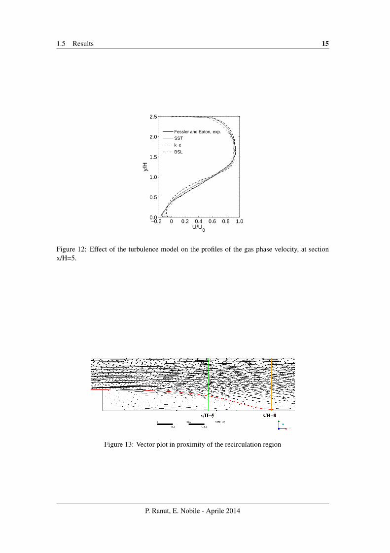
agree well with the experimental data, downstream the channel the deviation becomes moreconsistent. Besides the SST turbulence model, to which the previous results refer, two otherturbulence models were tested, i.e., the k−ε and the BSL. In Fig. 13 the effect of the turbulencemodel on the profiles of the gas phase velocity, at section x/H=5, is illustrated. While in theupper part of the section there is not a great difference among the the velocity profiles computedwith the different turbulence models, the SST model seems to predict better the profile in thelower part of the cross section. Furthermore, even the degree of turbulence was tested, but noeffect was registered on the results.In Table 3, the reattachment lengths predicted with the three tested turbulence models are com-pared with the experimental data [5] and the RANS results of [4]. As it can be seen, the predic-tion of the SST turbulence model are the closest to the experimental results. This fact encour-aged us to present only the results obtained with this turbulence model.


1.5 Results 13

−0.4 −0.2 0 0.2 0.4 0.6 0.8 1.00.0

0.5

1.0

1.5

2.0

2.5

U/U0

y/H

fluid

particles

(a)

−0.4 −0.2 0 0.2 0.4 0.6 0.8 1.00.0

0.5

1.0

1.5

2.0

2.5

U/U0

y/H

fluid

particles

(b)

−0.4 −0.2 0 0.2 0.4 0.6 0.8 1.00.0

0.5

1.0

1.5

2.0

2.5

U/U0

y/H

fluid

particles

(c)

−0.4 −0.2 0 0.2 0.4 0.6 0.8 1.00.0

0.5

1.0

1.5

2.0

2.5

U/U0

y/H

fluid

particles

(d)

Figure 10: CFX results for 70 µm copper particles at (a) x/H=2, (b) x/H=5, (c) x/H=7 and (d)x/H=9.

A vector plot in proximity of the recirculation region is illustrated in Fig. 14.


14 1.5 Results

−0.4 −0.2 0 0.2 0.4 0.6 0.8 1.00.0

0.5

1.0

1.5

2.0

2.5

U/U0

y/H

Fessler and Eaton,exp. 3%


Chan et al., RANS

Yu et al., LES

Present

(a)

−0.4 −0.2 0 0.2 0.4 0.6 0.8 1.00.0

0.5

1.0

1.5

2.0

2.5

U/U0

y/H



Chan et al., RANS

Yu et al., LES

Present

(b)

−0.4 −0.2 0 0.2 0.4 0.6 0.8 1.00.0

0.5

1.0

1.5

2.0

2.5

U/U0

y/H



Chan et al., RANS

Yu et al., LES

Present

(c)

−0.4 −0.2 0 0.2 0.4 0.6 0.8 1.00.0

0.5

1.0

1.5

2.0

2.5

U/U0

y/H



Chan et al., RANS

Yu et al., LES

Present

(d)

Figure 11: Stream-wise particulate phase mean velocity, for 70 µm copper particles. (a) x/H=2,(b) x/H=5, (c) x/H=7 and (d) x/H=9. Comparison with the results published in the literature.

x/H

Fessler and Eaton, [5] 7.6Chan et al. [4] 7.4Present, SST 7.42Present, k − ε 6.52Present, BSL 6.61

Table 3: Prediction of the reattachment length.


1.5 Results 15

−0.2 0 0.2 0.4 0.6 0.8 1.00.0

0.5

1.0

1.5

2.0

2.5

U/U0

y/H


SST

k−εBSL

Figure 12: Effect of the turbulence model on the profiles of the gas phase velocity, at sectionx/H=5.

Figure 13: Vector plot in proximity of the recirculation region


16 1.6 Comments

1.6 Comments

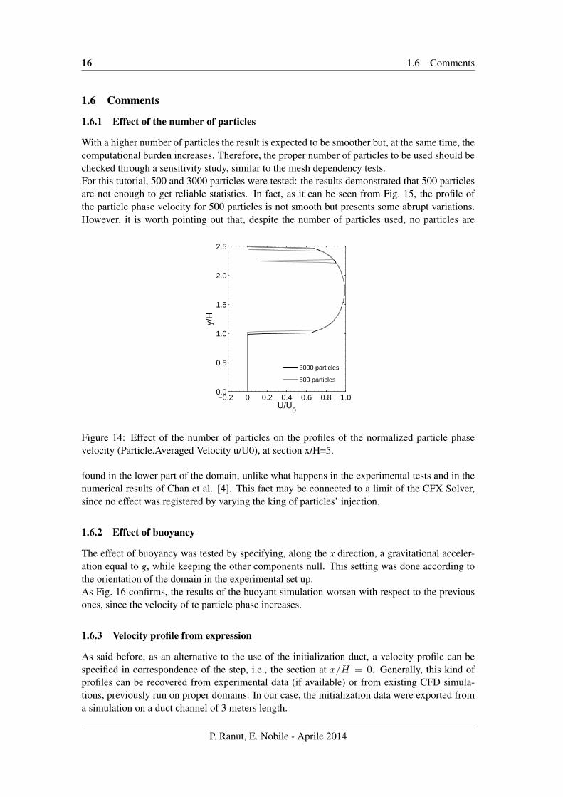
1.6.1 Effect of the number of particles

With a higher number of particles the result is expected to be smoother but, at the same time, thecomputational burden increases. Therefore, the proper number of particles to be used should bechecked through a sensitivity study, similar to the mesh dependency tests.For this tutorial, 500 and 3000 particles were tested: the results demonstrated that 500 particlesare not enough to get reliable statistics. In fact, as it can be seen from Fig. 15, the profile ofthe particle phase velocity for 500 particles is not smooth but presents some abrupt variations.However, it is worth pointing out that, despite the number of particles used, no particles are

−0.2 0 0.2 0.4 0.6 0.8 1.00.0

0.5

1.0

1.5

2.0

2.5

U/U0

y/H

3000 particles

500 particles

Figure 14: Effect of the number of particles on the profiles of the normalized particle phasevelocity (Particle.Averaged Velocity u/U0), at section x/H=5.

found in the lower part of the domain, unlike what happens in the experimental tests and in thenumerical results of Chan et al. [4]. This fact may be connected to a limit of the CFX Solver,since no effect was registered by varying the king of particles’ injection.

1.6.2 Effect of buoyancy

The effect of buoyancy was tested by specifying, along the x direction, a gravitational acceler-ation equal to g, while keeping the other components null. This setting was done according tothe orientation of the domain in the experimental set up.As Fig. 16 confirms, the results of the buoyant simulation worsen with respect to the previousones, since the velocity of te particle phase increases.

1.6.3 Velocity profile from expression

As said before, as an alternative to the use of the initialization duct, a velocity profile can bespecified in correspondence of the step, i.e., the section at x/H = 0. Generally, this kind ofprofiles can be recovered from experimental data (if available) or from existing CFD simula-tions, previously run on proper domains. In our case, the initialization data were exported froma simulation on a duct channel of 3 meters length.


1.6 Comments 17

0 0.2 0.4 0.6 0.8 1.0 1.20.0

0.5

1.0

1.5

2.0

2.5

U/U0

y/H

Non−buoyant

Buoyant

Figure 15: Effect of the buoyancy in x direction on the profiles of the normalized particle phasevelocity (Particle.Averaged Velocity u/U0), at section x/H=5.

Figure 16: Initialize profile data.

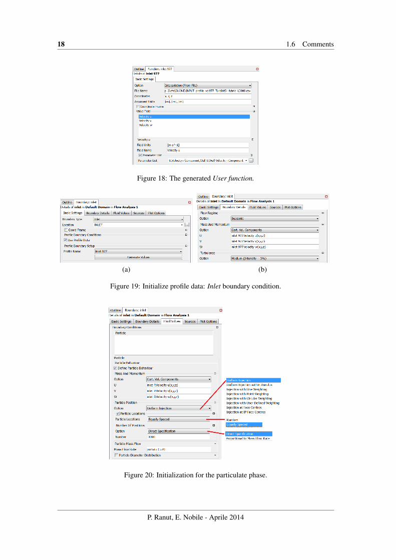
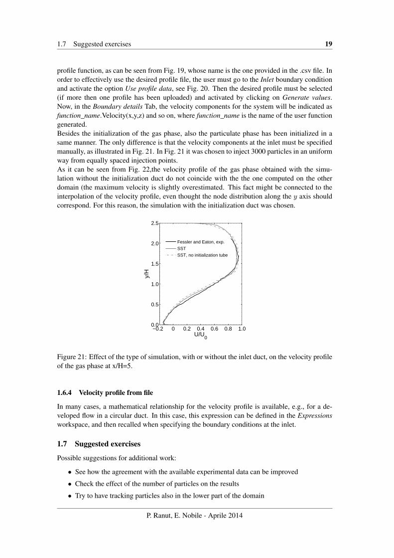
Figure 17: Structure of the initialization file .csv.

The specification of the velocity profile please refer to Fig. 17 and following. Go to Toolsand select Initialize Profile Data, then a dialog box appears. Hence select the file containingyour profile data, and click Open. The profile data is loaded and the profile data name, coordi-nates, variable names and units are displayed. The .csv file containing the initialization valuesmust be organized as illustrated in Fig. 18: a name must be provided for this profile (inlet 977in this case).Under the library section of the object tree, a new User Function object is generated for this


18 1.6 Comments

Figure 18: The generated User function.

(a) (b)

Figure 19: Initialize profile data: Inlet boundary condition.

Figure 20: Initialization for the particulate phase.


1.7 Suggested exercises 19

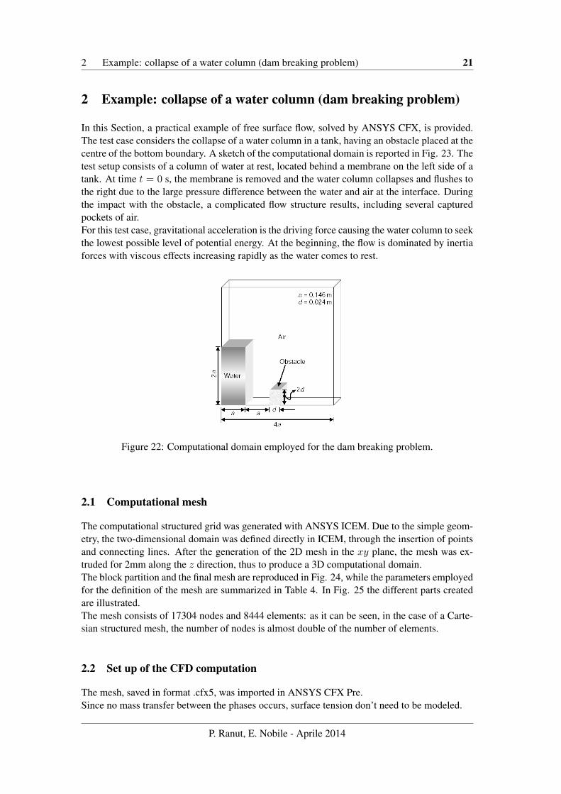
profile function, as can be seen from Fig. 19, whose name is the one provided in the .csv file. Inorder to effectively use the desired profile file, the user must go to the Inlet boundary conditionand activate the option Use profile data, see Fig. 20. Then the desired profile must be selected(if more then one profile has been uploaded) and activated by clicking on Generate values.Now, in the Boundary details Tab, the velocity components for the system will be indicated asfunction_name.Velocity(x,y,z) and so on, where function_name is the name of the user functiongenerated.Besides the initialization of the gas phase, also the particulate phase has been initialized in asame manner. The only difference is that the velocity components at the inlet must be specifiedmanually, as illustrated in Fig. 21. In Fig. 21 it was chosen to inject 3000 particles in an uniformway from equally spaced injection points.As it can be seen from Fig. 22,the velocity profile of the gas phase obtained with the simu-lation without the initialization duct do not coincide with the the one computed on the otherdomain (the maximum velocity is slightly overestimated. This fact might be connected to theinterpolation of the velocity profile, even thought the node distribution along the y axis shouldcorrespond. For this reason, the simulation with the initialization duct was chosen.

−0.2 0 0.2 0.4 0.6 0.8 1.00.0

0.5

1.0

1.5

2.0

2.5

U/U0

y/H


SST

SST, no initialization tube

Figure 21: Effect of the type of simulation, with or without the inlet duct, on the velocity profileof the gas phase at x/H=5.

1.6.4 Velocity profile from file

In many cases, a mathematical relationship for the velocity profile is available, e.g., for a de-veloped flow in a circular duct. In this case, this expression can be defined in the Expressionsworkspace, and then recalled when specifying the boundary conditions at the inlet.

1.7 Suggested exercises

Possible suggestions for additional work:

• See how the agreement with the available experimental data can be improved

• Check the effect of the number of particles on the results

• Try to have tracking particles also in the lower part of the domain


20 1.7 Suggested exercises

• Solve the problem by assuming a one-way coupling instead a two-way one, thus to verifywhether the results change and what it is the effect on the computational time

• Solve the problem in an Eulerian-Eulerian framework


2 Example: collapse of a water column (dam breaking problem) 21

2 Example: collapse of a water column (dam breaking problem)

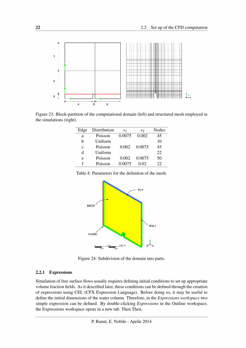
In this Section, a practical example of free surface flow, solved by ANSYS CFX, is provided.The test case considers the collapse of a water column in a tank, having an obstacle placed at thecentre of the bottom boundary. A sketch of the computational domain is reported in Fig. 23. Thetest setup consists of a column of water at rest, located behind a membrane on the left side of atank. At time t = 0 s, the membrane is removed and the water column collapses and flushes tothe right due to the large pressure difference between the water and air at the interface. Duringthe impact with the obstacle, a complicated flow structure results, including several capturedpockets of air.For this test case, gravitational acceleration is the driving force causing the water column to seekthe lowest possible level of potential energy. At the beginning, the flow is dominated by inertiaforces with viscous effects increasing rapidly as the water comes to rest.

Figure 22: Computational domain employed for the dam breaking problem.

2.1 Computational mesh

The computational structured grid was generated with ANSYS ICEM. Due to the simple geom-etry, the two-dimensional domain was defined directly in ICEM, through the insertion of pointsand connecting lines. After the generation of the 2D mesh in the xy plane, the mesh was ex-truded for 2mm along the z direction, thus to produce a 3D computational domain.The block partition and the final mesh are reproduced in Fig. 24, while the parameters employedfor the definition of the mesh are summarized in Table 4. In Fig. 25 the different parts createdare illustrated.The mesh consists of 17304 nodes and 8444 elements: as it can be seen, in the case of a Carte-sian structured mesh, the number of nodes is almost double of the number of elements.

2.2 Set up of the CFD computation

The mesh, saved in format .cfx5, was imported in ANSYS CFX Pre.Since no mass transfer between the phases occurs, surface tension don’t need to be modeled.


22 2.2 Set up of the CFD computation

Figure 23: Block-partition of the computational domain (left) and structured mesh employed inthe simulations (right).

Edge Distribution s1 s2 Nodesa Poisson 0.0075 0.002 45b Uniform 10c Poisson 0.002 0.0075 45d Uniform 22e Poisson 0.002 0.0075 50f Poisson 0.0075 0.02 22

Table 4: Parameters for the definition of the mesh.

Figure 24: Subdivision of the domain into parts.

2.2.1 Expressions

Simulation of free surface flows usually requires defining initial conditions to set up appropriatevolume fraction fields. As it described later, these conditions can be defined through the creationof expressions using CEL (CFX Expression Language). Before doing so, it may be useful todefine the initial dimensions of the water column. Therefore, in the Expressions workspace twosimple expression can be defined. By double-clicking Expressions in the Outline workspace,the Expressions workspace opens in a new tab. Then Then,


2.2 Set up of the CFD computation 23

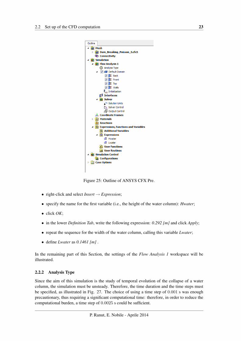
Figure 25: Outline of ANSYS CFX Pre.

• right-click and select Insert→ Expression;

• specify the name for the first variable (i.e., the height of the water column): Hwater;

• click OK;

• in the lower Definition Tab, write the following expression: 0.292 [m] and click Apply;

• repeat the sequence for the width of the water column, calling this variable Lwater;

• define Lwater as 0.1461 [m] .

In the remaining part of this Section, the settings of the Flow Analysis 1 workspace will beillustrated.

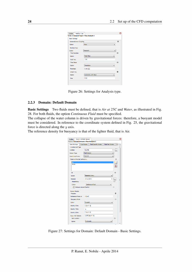
2.2.2 Analysis Type

Since the aim of this simulation is the study of temporal evolution of the collapse of a watercolumn, the simulation must be unsteady. Therefore, the time duration and the time steps mustbe specified, as illustrated in Fig. 27. The choice of using a time step of 0.001 s was enoughprecautionary, thus requiring a significant computational time: therefore, in order to reduce thecomputational burden, a time step of 0.0025 s could be sufficient.



Figure 26: Settings for Analysis type.

2.2.3 Domain: Default Domain

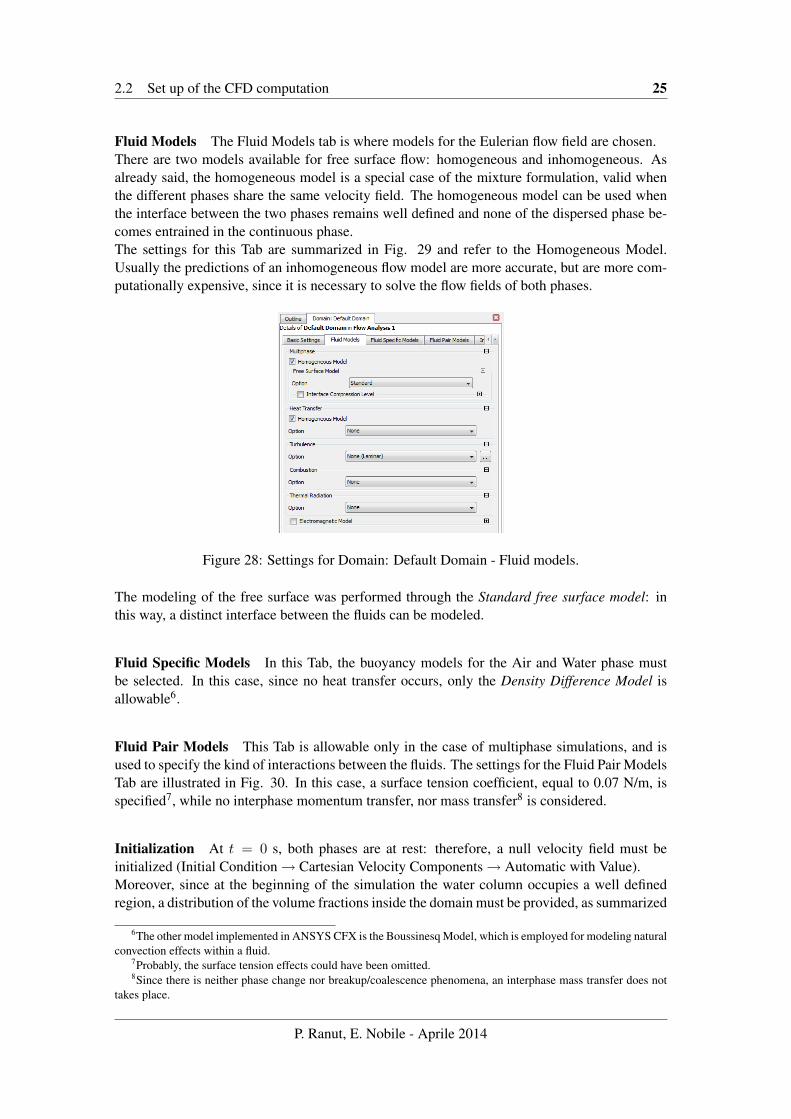
Basic Settings Two fluids must be defined, that is Air at 25C and Water, as illustrated in Fig.28. For both fluids, the option Continuous Fluid must be specified.The collapse of the water column is driven by gravitational forces: therefore, a buoyant modelmust be considered. In reference to the coordinate system defined in Fig. 25, the gravitationalforce is directed along the y axis.The reference density for buoyancy is that of the lighter fluid, that is Air.

Figure 27: Settings for Domain: Default Domain - Basic Settings.



Fluid Models The Fluid Models tab is where models for the Eulerian flow field are chosen.There are two models available for free surface flow: homogeneous and inhomogeneous. Asalready said, the homogeneous model is a special case of the mixture formulation, valid whenthe different phases share the same velocity field. The homogeneous model can be used whenthe interface between the two phases remains well defined and none of the dispersed phase be-comes entrained in the continuous phase.The settings for this Tab are summarized in Fig. 29 and refer to the Homogeneous Model.Usually the predictions of an inhomogeneous flow model are more accurate, but are more com-putationally expensive, since it is necessary to solve the flow fields of both phases.

Figure 28: Settings for Domain: Default Domain - Fluid models.

The modeling of the free surface was performed through the Standard free surface model: inthis way, a distinct interface between the fluids can be modeled.

Fluid Specific Models In this Tab, the buoyancy models for the Air and Water phase mustbe selected. In this case, since no heat transfer occurs, only the Density Difference Model isallowable6.

Fluid Pair Models This Tab is allowable only in the case of multiphase simulations, and isused to specify the kind of interactions between the fluids. The settings for the Fluid Pair ModelsTab are illustrated in Fig. 30. In this case, a surface tension coefficient, equal to 0.07 N/m, isspecified7, while no interphase momentum transfer, nor mass transfer8 is considered.

Initialization At t = 0 s, both phases are at rest: therefore, a null velocity field must beinitialized (Initial Condition→ Cartesian Velocity Components→ Automatic with Value).Moreover, since at the beginning of the simulation the water column occupies a well definedregion, a distribution of the volume fractions inside the domain must be provided, as summarized

6The other model implemented in ANSYS CFX is the Boussinesq Model, which is employed for modeling naturalconvection effects within a fluid.

7Probably, the surface tension effects could have been omitted.8Since there is neither phase change nor breakup/coalescence phenomena, an interphase mass transfer does not

takes place.



Figure 29: Settings for Domain: Default Domain - Fluid Pair Models.

in Fig. 31. This is done by specifying a logic expression as it follows:

if((x < Lwater)&&(y < Hwater), 0, 1) for Air (13)

if((x < Lwater)&&(y < Hwater), 1, 0) for Water (14)

The statement of a logic if condition is the following:

if(condition, value if it is true, value if it is false) (15)

Figure 30: Settings for Domain: Default Domain - Initialization - Fluid Specific Initialization

2.2.4 Boundary conditions

With reference to Fig. 25, the following boundary conditions were applied:

• Front: simmetry;

• Back: simmetry;

• Walls: no slip wall;

• Top: opening9

– Boundary details: Flow regime: subsonic; Mass and Momentum: Entrainment, Rel-ative Pressure: 0 Pa

9The opening boundary condition allow fluid to exit and enter the computational domain



– Fluid Values: Air, volume fraction: option: value, 1; Water, volume fraction: option:value, 0.

The setting of an opening boundary condition allow to free from the interaction of the waterwith the upper wall (if some particles reach the top boundary, they escape from the domain).

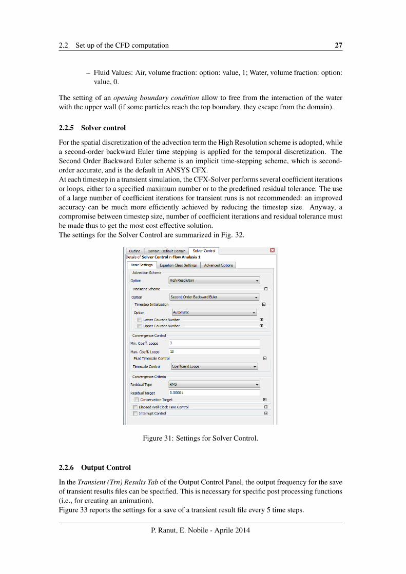
2.2.5 Solver control

For the spatial discretization of the advection term the High Resolution scheme is adopted, whilea second-order backward Euler time stepping is applied for the temporal discretization. TheSecond Order Backward Euler scheme is an implicit time-stepping scheme, which is second-order accurate, and is the default in ANSYS CFX.At each timestep in a transient simulation, the CFX-Solver performs several coefficient iterationsor loops, either to a specified maximum number or to the predefined residual tolerance. The useof a large number of coefficient iterations for transient runs is not recommended: an improvedaccuracy can be much more efficiently achieved by reducing the timestep size. Anyway, acompromise between timestep size, number of coefficient iterations and residual tolerance mustbe made thus to get the most cost effective solution.The settings for the Solver Control are summarized in Fig. 32.

Figure 31: Settings for Solver Control.

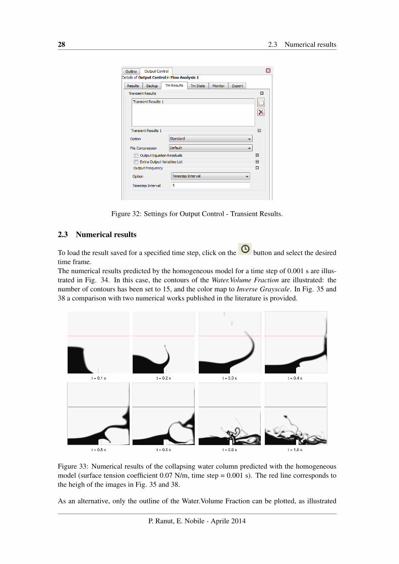
2.2.6 Output Control

In the Transient (Trn) Results Tab of the Output Control Panel, the output frequency for the saveof transient results files can be specified. This is necessary for specific post processing functions(i.e., for creating an animation).Figure 33 reports the settings for a save of a transient result file every 5 time steps.


28 2.3 Numerical results

Figure 32: Settings for Output Control - Transient Results.

2.3 Numerical results

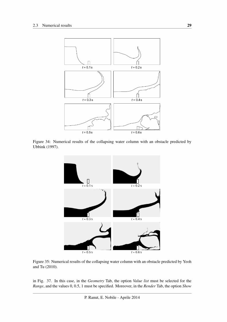
To load the result saved for a specified time step, click on the button and select the desiredtime frame.The numerical results predicted by the homogeneous model for a time step of 0.001 s are illus-trated in Fig. 34. In this case, the contours of the Water.Volume Fraction are illustrated: thenumber of contours has been set to 15, and the color map to Inverse Grayscale. In Fig. 35 and38 a comparison with two numerical works published in the literature is provided.

Figure 33: Numerical results of the collapsing water column predicted with the homogeneousmodel (surface tension coefficient 0.07 N/m, time step = 0.001 s). The red line corresponds tothe heigh of the images in Fig. 35 and 38.

As an alternative, only the outline of the Water.Volume Fraction can be plotted, as illustrated


2.3 Numerical results 29

Figure 34: Numerical results of the collapsing water column with an obstacle predicted byUbbink (1997).

Figure 35: Numerical results of the collapsing water column with an obstacle predicted by Yeohand Tu (2010).

in Fig. 37. In this case, in the Geometry Tab, the option Value list must be selected for theRange, and the values 0, 0.5, 1 must be specified. Moreover, in the Render Tab, the option Show


30 2.3 Numerical results

Contours Bands must be unchecked. To draw the contour with line of a specified color, expandthe Show Surface Lines options, and check the option Constant Coloring→ User Specified.

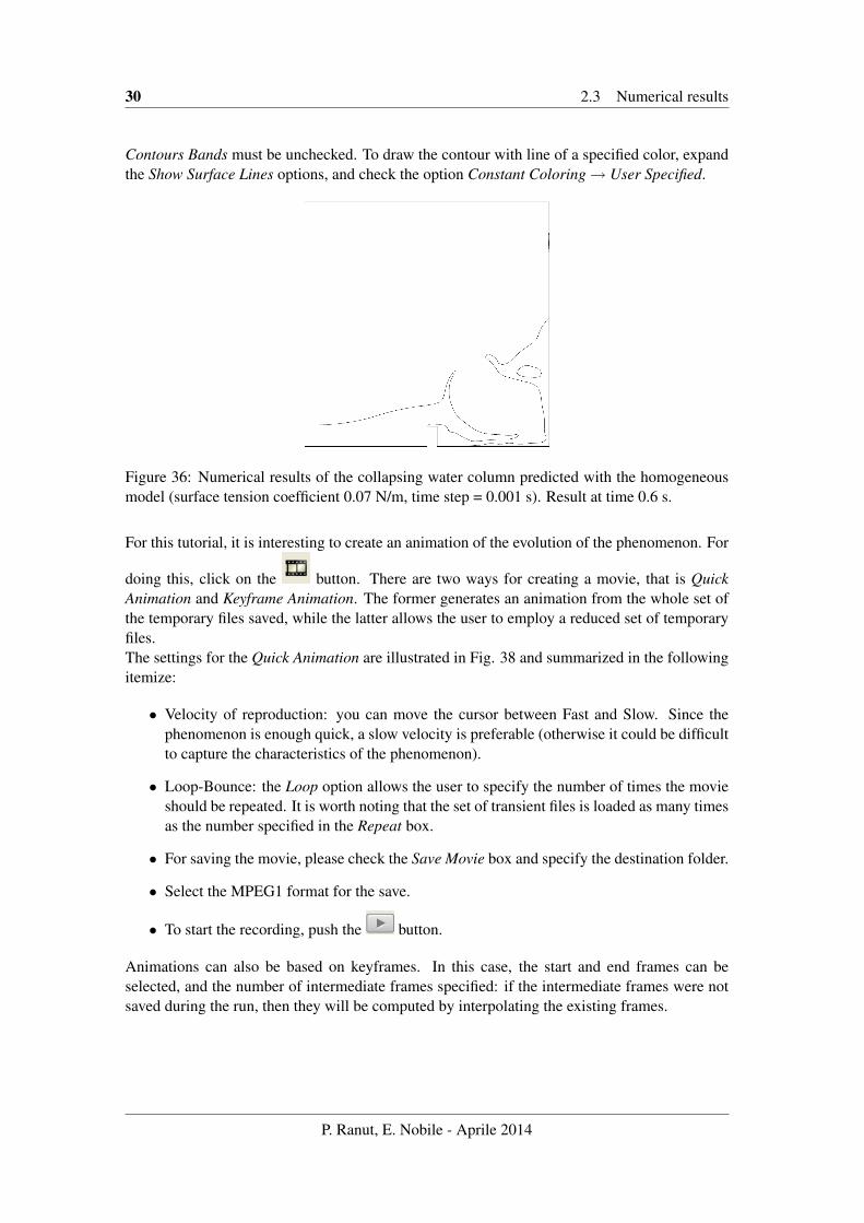
Figure 36: Numerical results of the collapsing water column predicted with the homogeneousmodel (surface tension coefficient 0.07 N/m, time step = 0.001 s). Result at time 0.6 s.

For this tutorial, it is interesting to create an animation of the evolution of the phenomenon. For

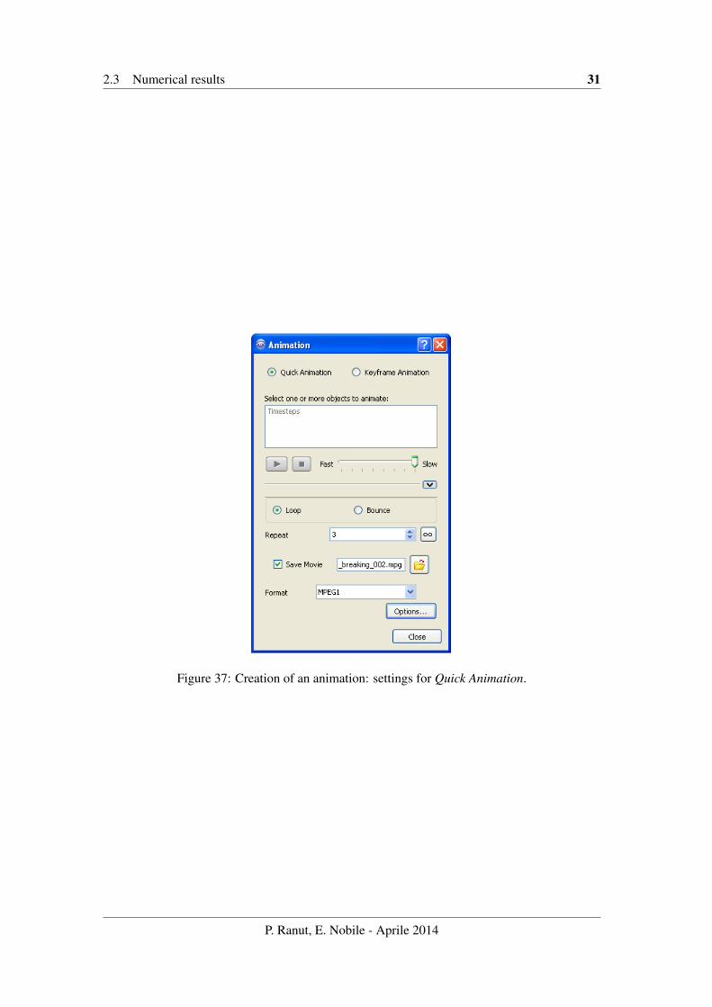
doing this, click on the button. There are two ways for creating a movie, that is QuickAnimation and Keyframe Animation. The former generates an animation from the whole set ofthe temporary files saved, while the latter allows the user to employ a reduced set of temporaryfiles.The settings for the Quick Animation are illustrated in Fig. 38 and summarized in the followingitemize:

• Velocity of reproduction: you can move the cursor between Fast and Slow. Since thephenomenon is enough quick, a slow velocity is preferable (otherwise it could be difficultto capture the characteristics of the phenomenon).

• Loop-Bounce: the Loop option allows the user to specify the number of times the movieshould be repeated. It is worth noting that the set of transient files is loaded as many timesas the number specified in the Repeat box.

• For saving the movie, please check the Save Movie box and specify the destination folder.

• Select the MPEG1 format for the save.

• To start the recording, push the button.

Animations can also be based on keyframes. In this case, the start and end frames can beselected, and the number of intermediate frames specified: if the intermediate frames were notsaved during the run, then they will be computed by interpolating the existing frames.


2.3 Numerical results 31

Figure 37: Creation of an animation: settings for Quick Animation.


32 REFERENCES

References

[1] A. Benavides and B. van Wachem. Eulerian-eulerian prediction of dilute turbulent gas-particle flow in a backward-facing step. Int. J. Heat Fluid Flow, 30:452–461, 2009.

[2] M.S. Bhatti and R.K. Shah. Turbulent and transition flow convective heat transfer in ducts.In S. Kakaç, R.K. Shah, and W. Aung, editors, Handbook of Single-Phase Convective HeatTransfer. John Wiley & sons, 1987.

[3] G. Biswas, M. Breuer, and F. Durst. Backward-facing step flows for various expansionratios at low and moderate reynolds numbers. J. Fluids Eng., 126:362–374, 2004.

[4] C.K. Chan, H.Q. Zhang, and K.S. Lau. Numerical simulation of gas-particle flows behinda backward-facing step using an improved stochastic separated flow model. ComputationalMechanics, 27:412–417, 2001.

[5] J.R. Fessler and J.K. Eaton. Turbulence modification by particles in a backward-facing stepflow. J. Fluid Mesh., 394:97–117, 1999.

[6] K.F. Yu, K.S. Lau, and C.K. Chan. Numerical simulation of gas-particle flow in a single-sidebackward-facing step flow. Journal of Computational and Applied Mathematics, 163:319–331, 2004.


multiphase ﬂows examples solved with ansys cfx

Documents