direct numerical simulations of gas-liquid multiphase flows · in a large number of applications...
TRANSCRIPT

Direct Numerical Simulations of Gas-Liquid
Multiphase Flows
Gretar Tryggvason, Ruben Scardovelli and Stephane Zaleski

1
Introduction
Gas-liquid multiphase flows play an essential role in the workings of Na-ture and the enterprises of mankind. Our everyday encounter with liquidsis nearly always at a free surface, such as when drinking, washing, rinsingand cooking. Similarly, such flows are in abundance in industrial applica-tions: heat transfer by boiling is the preferred mode in both conventionaland nuclear power plants and bubble driven circulation systems are used inmetal processing operations such as steel making, ladle metallurgy and thesecondary refining of aluminum and copper. A significant fraction of theenergy needs of mankind is met by burning liquid fuel and a liquid mustevaporate before it burns. In almost all cases the liquid is therefore atom-ized to generate a large number of small droplets and hence a large surfacearea. Indeed, except for drag (including pressure drops in pipes) and mixingof gaseous fuels we would not be far off to assert that nearly all industrialapplications of fluids involve a multiphase flow of one sort or another. Some-times, one of the phases is a solid, such as in slurries and fluidized beds, butin a large number of applications one phase is a liquid and the other is a gas.Of natural gas-liquid multiphase flows, rain is perhaps the experience thatfirst comes to mind, but bubbles and droplets play a major role in the ex-change of heat and mass between oceans and the atmosphere and in volcanicexplosions. Living organisms are essentially large and complex multiphasesystems.
Understanding the dynamics of gas-liquid multiphase flows is of criticalengineering and scientific importance and the literature is extensive. Froma mathematical point of view multiphase flow problems are notoriously dif-ficult and much of what we know has been obtained by experimentation andscaling analysis. Not only are the equations, governing the fluid flow in bothphases, highly nonlinear, but the position of the phase boundary must gen-erally be found as a part of the solution. Exact analytical solutions therefore
11

12 Introduction
Fig. 1.1. A picture of many buoyant bubbles rising in an otherwise quiescent liq-uid pool. The average bubble diameter is about 2.2 mm and the void fractionis approximately 0.75%. From Broder and Sommerfeld (2007). Reproduced withpermission.
exist only for the simplest problems such as the steady-state motion of bub-bles and droplets in Stokes flow, linear inviscid waves and small oscillationsof bubbles and droplets. Experimental studies of multiphase flows are noteasy either. For many flows of practical interest the length scales are small,the time scales are short and optical access to much of the flow is limited.The need for numerical solutions of the governing equations has thereforebeen felt by the multiphase research community since the origin of computa-tional fluid dynamics, in the late fifties and early sixties. Although much hasbeen accomplished, simulations of multiphase flows have remained far be-hind homogeneous flows where direct numerical simulations (DNS)—wherethe governing equations are solved using sufficiently fine grids so that allcontinuum time- and length-scales are fully resolved—have become a stan-dard tool in turbulence research. While this is not surprising, consideringthe added difficulty, the situation is certainly not due to lack of effort. How-ever, in the last decade and a half or so, these efforts have started to pay offand rather significant progress has been accomplished on many fronts. It isnow possible to do DNS for a large number of fairly complex systems and

1.1 Examples of multiphase flows 13
Fig. 1.2. A photograph of an atomization experiment performed with coaxial waterand air jets reproduced from Villermaux et al. (2004). Reproduced with permission.Copyright American Physical Society.
DNS are starting to yield information that are likely to be unobtainable inany other way. This book is an effort to assess the state-of-the-art, to re-view how we came to where we are and to provide the foundation to furtherprogress, for even more complex multiphase flows.
1.1 Examples of multiphase flows
Since this is a book about numerical simulations, it seems appropriate tostart by showing a few “real” systems. The following examples are pickedsomewhat randomly, but give some insight into the kind of systems that canbe examined by direct numerical simulations.
Bubbles are found in a large number of industrial applications. For exam-ple they carry vapor away from hot surfaces in boiling heat transfer, dispersegasses and provide stirring in various chemical processing systems and alsoaffect the propagation of sound in the ocean. To design systems that involvebubbly flows it is necessary to understand how the collective rise velocity ofmany bubbles depends on the void fraction and the bubble size distribution,how bubbles disperse and how they stir up the fluid. Figure 1.1 is a pictureof air bubbles rising through water in a small bubble column. The averagebubble diameter is about 2.2 mm and the void fraction is approximately0.75%. At these parameters the bubbles rise with an average velocity of

14 Introduction
Fig. 1.3. The splash generated when a droplet hits a free surface. From A. David-hazy. Rochester Institute of Technology. Reproduced with permission.
roughly 0.27 m/s, but since the bubbles are not all of the same size theywill generally rise with different velocities.
To generate sprays for combustion, coating and painting, irrigation, hu-midification and a large number of other applications a liquid jet must beatomized. Predicting the rate of atomization and the resulting droplet sizedistribution, as well as their velocity, is critical to the successful design ofsuch processes. In Fig. 1.2, a liquid jet is ejected from a nozzle of diameter 8mm with a velocity of 0.6 m/s. To accelerate its breakup, the jet is injectedinto a co-flowing air stream, with a velocity of 35 m/s. Initially, the shearbetween the air and the liquid leads to large axisymmetric waves but as thewaves move downstream the air pulls long filaments from the crest of thewave. The filaments then break into droplets by a capillary instability. SeeMarmottant and Villermaux (2001) and Villermaux et al. (2004) for details.
Droplets impacting solid or liquid surfaces generally splash, often disrupt-ing the surface significantly. Rain droplets falling on the ground often resultin soil erosion, for example. But droplet impact can also help to increase theheat transfer, such as in quenching and spray cooling, and rain often greatlyenhances the mixing at the ocean surface. Figure 1.3 shows the splash cre-ated when a droplet of a diameter of about three millimeters, released from

1.1 Examples of multiphase flows 15
Fig. 1.4. Massive cavitation near the leading edge of an airfoil. The flow is fromthe left to right. From Kermeen (1956). Reproduced with permission.
nearly half a meter above the surface, impacts a liquid layer a little over adroplet-diameter deep. The impact of the droplet creates a liquid crater anda rim that often breaks into droplets. As the crater collapses, air bubblesare sometimes trapped in the liquid.
While bubbles are often generated by air injection into a pool of liquidor are formed by entrainment at a free surface, such as when waves break,they also frequently form when a liquid changes phase into vapor. Such aphase change is often nucleated at a solid surface and can take place eitherby heating the liquid above the saturation temperature, as in boiling, orby lowering the pressure below the vapor pressure, as in cavitation. Figure1.4 shows massive cavitation at the leading edge of an airfoil submerged inwater. The chord of the airfoil is 7.6 cm, the flow speed is 13.7 m/s from leftto right, and the increase in the liquid velocity as it passes over the leadingedge of the airfoil leads to a drop in pressure that is sufficiently large so thatthe liquid “boils”. As the vapor bubbles move into regions of higher pressureat the back of the airfoil, they collapse. However, residual gases, dissolvedin the liquid, diffuse into the bubbles during their existence, leaving tracesthat are visible after the vapor has condensed.
In many multiphase systems one phase is a solid. Suspensions of solidparticles in liquids or gases are common and the definition of multiphaseflows is sometimes extended to cover flows through or over complex station-ary solids, such as packed beds, porous media, forests and cities. The main

16 Introduction
Fig. 1.5. Microstructure of an aluminum-silicon alloy. From D. Apelian, WorcesterPolytechnic Institute. Reproduced with permission.
difference between gas-liquid multiphase flows and solid-gas and solid-liquidmultiphase flows is usually that the interface maintains its shape in the lattercases, even though the location of the solid may change. In some instances,however, that is not the case. Flexible solids can change their shape in re-sponse to fluid flow and during solidification or erosion the boundary canevolve, sometimes into shapes that are just as convoluted as encounteredfor gas-liquid systems. When a metal alloy solidifies, the solute is initiallyrejected by the solid phase. This leads to constitutional undercooling andan instability of the solidification front. The solute-rich phase eventually so-lidifies, but with a very different composition than the material that first be-came solid. The size, shape and composition of the resulting microstructuresdetermine the properties of the material and those are usually sensitively de-pendent on the various process parameters. A representative micrograph ofan Al-Si alloy prepared by metallographic techniques and etching to revealphase boundaries and interfaces is shown in Fig. 1.5. The light gray phaseis almost pure aluminum and solidifies first, but constitutional undercoolingleads to dendritic structures of a size measured in few tens of micrometers.
Living systems provide an abundance of multiphase flow examples. Sus-pended blood cells and aerosol in pulmonary flow are obvious examples atthe “body” scale, as are the motion of organs and even complete individu-

1.2 Computational modeling 17
Fig. 1.6. A school of yellow-tailed goatfish (Mulloidichthys flavolineatus) near theNorthwest Hawaiian Islands. From the NOAA Photo Library.
als. But even more complex systems, such as the motion of a flock of birdsthrough air and a school of fish through water, are also multiphase flows.Figure 1.6 show a large number of yellow-tailed goatfish swimming togetherand coordinating their movement. An understanding of the motion of botha single fish as well as the collective motion of a large school may have im-plication for population control and harvesting, as well as the constructionof mechanical swimming and flying devices.
1.2 Computational modeling
Computations of multi-fluid (two different fluids) and multiphase (samefluid, different phases) flows are nearly as old as computations of constant-density flows. As for such flows, a number of different approaches have beentried and a number of simplifications used. In this section we will attemptto give a brief but comprehensive overview of the major efforts to simulatemulti-fluid flows. We make no attempt to cite every paper, but hope tomention all major developments.

18 Introduction
1.2.1 Simple flows (Re=0 and Re=∞)
In the limit of either very large or very small viscosity (as measured bythe Reynolds number, see Chapter 2.2.6), it is sometimes possible to sim-plify considerably the flow description by either ignoring inertia completely(Stokes flow) or by ignoring viscous effects completely (inviscid flow). Forinviscid flows it is usually further necessary to assume that the flow is irrota-tional, except at fluid interfaces. Most success has been achieved for disperseflows of undeformable spheres where, in both these limits, it is possible toreduce the governing equations to a system of coupled ordinary differentialequations (ODEs) for the particle positions. For Stokes flow the main de-veloper was Brady and his collaborators (see Brady and Bossis, 1988, fora review of early work) who have investigated extensively the properties ofsuspensions of particles in shear flows, among other problems. For inviscidflows, Sangani and Didwania (1993) and Smereka (1993) simulated the mo-tions of spherical bubbles in a periodic box and observed that the bubblestended to form horizontal clusters, particularly when the variance of thebubble velocity was small.
For both Stokes flows and inviscid potential flows, problems with de-formable boundaries can be simulated with boundary integral techniques.One of the earliest attempts was due to Birkhoff (1954) where the evolutionof the interface between a heavy fluid initially on top of a lighter one (theRayleigh-Taylor instability) was followed by a method tracking the interfacebetween two inviscid and irrotational fluids. Both the method and the prob-lem later became a staple of multiphase flow simulations. A boundary inte-gral method for water waves was presented by Longuet-Higgins and Cokelet(1976) and used to examine breaking waves. This paper had enormous in-fluence and was followed by a large number of very successful extensions andapplications, particularly for water waves (Baker et al., 1982; Vinje and Bre-vig, 1981; Schultz et al., 1994, and others). Other applications include theevolution of the Rayleigh-Taylor instability (Baker et al., 1980), the growthand collapse of cavitation bubbles (Blake and Gibson, 1981; Robinson et al.,2001), the generation of bubbles and droplets due to the coalescence of bub-bles with a free surface (Oguz and Prosperetti, 1990; Boulton-Stone andBlake, 1993), the formation of bubbles and droplets from an orifice (Oguzand Prosperetti, 1993) and the interactions of vortical flows with a free sur-face (Yu and Tryggvason, 1990), just to name a few. All boundary integral(or boundary element, when the integration is element based) methods forinviscid flows are based on following the evolution of the strength of surfacesingularities in time by integrating a Bernoulli-type equation. The surface

1.2 Computational modeling 19
Fig. 1.7. A Stokes flow simulation of the breakup of a droplet in a linear shear flow.The barely visible line behind the numerical results is the outline of a drop tracedfrom an experimental photograph. Reprinted with permission from Cristini et al.(1998). Copyright 2005, American Institute of Physics.
singularities give one velocity component and Green’s second theorem yieldsthe other, thus allowing the position of the surface to be advanced in time.Different surface singularities allow for a large number of different methods(some that can only deal with a free surface and others that are suited fortwo-fluid problems) and different implementations multiply the possibilitieseven further. For an extensive discussion and recent progress see Hou et al.(2001). Although continuous improvements are being made and new appli-cations continue to appear, two-dimensional boundary integral techniquesfor inviscid flows are by now—more than thirty years after the publicationof the paper by Longuett-Higgins and Cokelet—a fairly mature technology.Fully three-dimensional computations are, however, still rare. Chahine andDuraiswami (1992) computed the interactions of a few inviscid cavitationbubbles and Xue et al. (2001) have simulated a three-dimensional breakingwave. While the potential flow assumption has lead to many spectacularsuccesses, particularly for short-time transient flows, its inherent limitationsare many. The lack of a small-scale dissipative mechanism makes thosemodels susceptible to singularity formation and the absence of dissipationusually makes them unsuitable for the predictions of the long-time evolutionof any system.
20 Introduction
The key to the reformulation of inviscid interface problems with irrota-tional flow in terms of a boundary integral is the linearity of the potentialequation. In the opposite limit, where inertia effects can be ignored andthe flow is dominated by viscous dissipation, the Navier-Stokes equationsbecome linear (it is the so-called Stokes flow limit) and it is also possible torecast the governing equations into an integral equation on a moving surface.Boundary integral simulations of unsteady two-fluid Stokes problems origi-nated with Youngren and Acrivos (1976) and Rallison and Acrivos (1978),who simulated the deformation of a bubble and a droplet, respectively, in anextensional flow. Subsequently, several authors have investigated a numberof problems. Pozrikidis and collaborators have examined several aspects ofsuspensions of droplets, starting with a study by Zhou and Pozrikidis (1993)of the suspension of a few two-dimensional droplets in a channel. Simula-tions of fully three-dimensional suspensions have been done by Loewenbergand Hinch (1996) and Zinchenko and Davis (2000). The method has beendescribed in detail in the book by Pozrikidis (1992), and Pozrikidis (2001)gives a very complete summary of the various applications. An example ofa computation of the breakup of a very viscous droplet in a linear shearflow, using a method that adaptively refines the surface grid as the dropletdeforms is shown in Fig. 1.7.
In addition to inviscid flows and Stokes flows, boundary integral methodshave been used by a number of authors to examine two-dimensional, two-fluid flows in Hele-Shaw cells. Although the flow is completely viscous, awayfrom the interface it is a potential flow. The interface can be representedby the singularities used for inviscid flows (de Josselin de Jong, 1960) butthe evolution equation for the singularity strength is different. This wasused by Tryggvason and Aref (1983) and Tryggvason and Aref (1985) toexamine the Saffman-Taylor instability, where an interface separating twofluids of different viscosity deforms if the less viscous fluid is displacing themore viscous one. They used a fixed grid to solve for the normal velocitycomponent (instead of Green’s theorem), but Green’s theorem was subse-quently used by several authors to develop boundary integral methods forinterfaces in Hele-Shaw cells. See, for example, DeGregoria and Schwartz(1985), Meiburg and Homsy (1988) and the review by Hou et al. (2001).
Under the heading of simple flows we should also mention simulations ofthe motion of solid particles, in the limit where the fluid motion can beneglected and the dynamics is governed only by the inertia of the particles.Several authors have followed the motion of a large number of particles thatinteract only when they collide with each other. Here, it is also sufficientto solve a system of ODEs for the particle motion. Simulations of this
1.2 Computational modeling 21
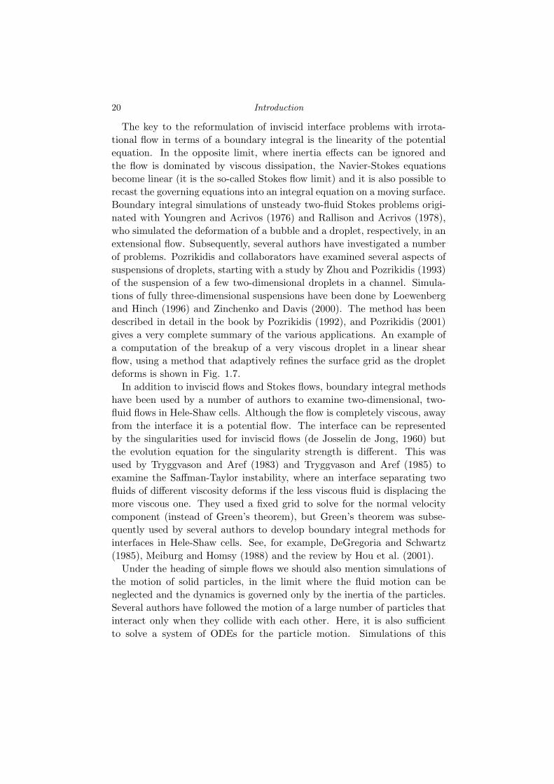
Fig. 1.8. The beginnig of computational studies of multiphase flows. The evolutionof the nonlinear Rayleigh-Taylor instability, computed using the two fluid MACmethod. Reprinted with permission from Daly (1969b). Copyright 2005, AmericanInstitute of Physics.
kind are usually called “granular dynamics.” For an early discussion seeLouge (1994) and a more recent one can be found in Poschel and Schwage(2005), for example. While these methods have been enormously successfulin simulating certain types of solid-gas multiphase flows, they are limited toa very small class of problems. One could, however, argue that simulations ofthe motion of particles interacting through a potential, such as simulations ofthe gravitational interactions of planets or galaxies and molecular dynamics,also fall into this class. Discussing such methods and their applicationswould enlarge the scope of the present work enormously and we will confineour coverage by simply suggesting that the interested reader consults theappropriate references, such as Schlick (2002) for molecular simulations andHockney and Eastwood (1981) for astrophysical and other systems.
1.2.2 Finite Reynolds number flows
For intermediate Reynolds numbers it is necessary to solve the full Navier-Stokes equations. Nearly ten years after Birkhoff’s effort to simulate theinviscid Rayleigh-Taylor problem by a boundary integral technique, theMarker-and-Cell (MAC) method was developed at Los Alamos by Harlowand collaborators. In the MAC method the fluid is identified by marker par-ticles distributed throughout the fluid region and the governing equationssolved on a regular grid that covers both the fluid-filled and the empty partof the domain. The method was introduced in Harlow and Welch (1965)

22 Introduction
and two sample computations of the so-called dam breaking problem wereshown in that first paper. Several papers quickly followed: Harlow andWelch (1966) examined the Rayleigh-Taylor problem (Fig. 1.8) and Harlowand Shannon (1967) studied the splash when a droplet hits a liquid surface.As originally implemented, the MAC method assumed a free surface so therewas only one fluid involved. This required boundary conditions to be ap-plied at the surface and the fluid in the rest of the domain to be completelypassive. The Los Alamos group realized, however, that the same method-ology could be applied to two-fluid problems. Daly (1969b) computed theevolution of the Rayleigh-Taylor instability for finite density ratios and Dalyand Pracht (1968) examined the initial motion of density currents. Surfacetension was then added by Daly (1969a) and the method again used to ex-amine the Rayleigh-Taylor instability. The MAC method quickly attracteda small group of followers that used it to study several problems: Chan andStreet (1970) applied it to free surface waves, Foote (1973) and Foote (1975)simulated the oscillations of an axisymmetric droplet and the collision of adroplet with a rigid wall, respectively, and Chapman and Plesset (1972) andMitchell and Hammitt (1973) followed the collapse of a cavitation bubble.While the Los Alamos group did a number of computations of various prob-lems in the sixties and early seventies and Harlow described the basic ideain a Scientific American article (Harlow and Fromm, 1965), the enormouspotential of this newfound tool did not, for the most part, capture the fancyof the fluid mechanics research community. Although the MAC method wasdesigned specifically for multifluid problems (hence the M for Markers!) itwas also the first method to successfully solve the Navier-Stokes equation us-ing the primitive variables (velocity and pressure). The staggered grid usedwas a novelty and today it is a common practice to refer to any methodusing a projection based time integration on a staggered grid as a MACmethod (see Chapter 3).
The next generation of methods for multifluid flows evolved graduallyfrom the MAC method. It was already clear in the Harlow and Welch(1965) paper that the marker particles could cause inaccuracies and of themany algorithmic ideas explored by the Los Alamos group, the replacementof the particles by a marker function soon became the most popular alter-native. Thus the Volume-of-Fluid (VOF) method was born. VOF was firstdiscussed in a refereed journal article by Hirt and Nichols (1981) but themethod originated earlier (DeBar, 1974; Noh and Woodward, 1976). Thebasic problem with advecting a marker function is the numerical diffusionresulting from working with a cell-averaged marker function (see Chapter4). To prevent the marker function from continuing to diffuse, the inter-

1.2 Computational modeling 23
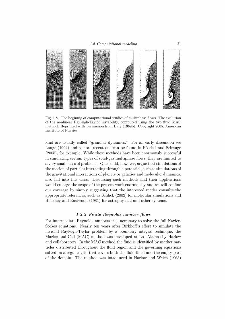
face is “reconstructed” in the VOF method in such a way that the markerdoes not start to flow into a new cell until the current cell is full. Theone-dimensional implementation of this idea is essentially trivial and in theearly implementation of VOF, the interface in each cell was simply assumedto be a vertical plane for advection in the horizontal direction and a hor-izontal plane for advection in the vertical direction. This relatively crudereconstruction often lead to large amount of “floatsam and jetsam” (smallunphysical droplets that break away from the interface) that degraded theaccuracy of the computation. To improve the representation, Youngs (1982)and Ashgriz and Poo (1991) and others introduced more complex recon-structions of the interface, representing it with a line (two dimensions) or aplane (three dimensions) that could be oriented arbitrarily in such a way asto best fit the interface. This increased the complexity of the method con-siderably but resulted in greatly improved advection of the marker function.Even with higher-order representation of the fluid interface in each cell, theaccurate computation of surface tension remained a major problem. In hissimulations of surface tension effects on the Rayleigh-Taylor instability, us-ing the MAC method, Daly (1969b) introduced explicit surface markers forthis purpose. However, the premise behind the development of the VOFmethod was to get away from using any kind of surface marker so that thesurface tension had to be obtained from the marker function instead. Thiswas achieved by Brackbill et al. (1992) who showed that the curvature (andhence surface tension) could be computed by taking the discrete divergenceof the marker function. A “conservative” version of this “continuum surfaceforce” method was developed by Lafaurie et al. (1994). The VOF methodhas been extended in various ways by a number of authors. In addition tobetter ways to reconstruct the interface (Rider and Kothe, 1998; Scardovelliand Zaleski, 2000; Aulisa et al., 2007) and compute the surface tension (Re-nardy and Renardy, 2002; Popinet, 2009), more advanced advection schemesfor the momentum equation and better solvers for the pressure equation havebeen introduced (see Rudman, 1997, for example). Other refinement includethe use of sub-cells to keep the interface as sharp as possible (Chen et al.,1997a). VOF methods are in widespread use today and many commercialcodes include VOF to track interfaces and free surfaces. Figure 1.9 showsone example of a computation of the splash made when a liquid droplet hitsa free surface, done by a modern VOF method. We will discuss the use ofVOF extensively in later Chapters.
The basic ideas behind the MAC and the VOF methods gave rise toseveral new approaches in the early nineties. Unverdi and Tryggvason (1992)introduced a Front-Tracking method for multifluid flows where the interface
24 Introduction
Fig. 1.9. Computation of splashing droplets using an advanced VOF method.Reprinted from Rieber and Frohn (1999) with permission from Elsevier.
was marked by connected marker points. The markers are used to advect thematerial properties (such as density and viscosity) and to compute surfacetension, but the rest of computations is done on a fixed grid as in the VOFmethod. Although using connected markers to update the material functionwas new, marker particles had already been used by Daly (1969a) who usedthem to evaluate surface tension in simulations with the MAC method, inthe Immersed-Boundary Method of Peskin (1977) for one-dimensional elasticfibers in homogeneous viscous fluids and in the Vortex-in-Cell method ofTryggvason and Aref (1983) for two-fluid interfaces in a Hele-Shaw cell, forexample. The Front-Tracking method of Unverdi and Tryggvason (1992)has been very successful for simulations of finite Reynolds number flows ofimmiscible fluids and Tryggvason and collaborators have used it to explorea large number of problems.
The early nineties also saw the introduction of the Level-Set, the CIP,and the Phase-Field methods to track fluid interfaces on stationary grids.The Level-Set method was introduced by Osher and Sethian (1988), but itsfirst use to track fluid interfaces appears to be in the work of Sussman et al.(1994) and Chang et al. (1996) who used it to simulate the rise of bubblesand the fall of droplets in two-dimensions. An axisymmetric version wasused subsequently by Sussman and Smereka (1997) to examine the behaviorof bubbles and droplets. Unlike the VOF method, where a discontinuousmarker function is advected with the flow, in the Level-Set method a contin-uous level-set function is used. The interface is then identified with the zero

1.2 Computational modeling 25
contour of the level-set function. To reconstruct the material properties ofthe flow (density and viscosity, for example) a marker function is constructedfrom the level-set function. The marker function is given a smooth transitionzone from one fluid to the next, thus increasing the regularity of the interfaceover the VOF method where the interface is confined to only one grid space.However, this mapping from the level-set function to the marker functionrequires the level-set function to maintain the same shape near the interfaceand to deal with this problem, Sussman et al. (1994) introduced a reinitial-ization procedure where the level-set function is adjusted in such a way thatits value is equal to the shortest distance to the interface at all times. Thisstep was critical in making level-sets work for fluid-dynamics simulations.Surface tension is found in the same way as in the continuous surface forcetechnique introduced for VOF methods by Brackbill et al. (1992). The earlyimplementation of the Level-Set method did not conserve mass very well anda number of improvements and extension followed its original introduction.Sussman et al. (1998) and Sussman and Fatemi (1999) introduced ways toimproved mass conservation, Sussman et al. (1999) coupled level-set track-ing with adaptive grid refinement and a hybrid VOF/Level-Set method wasdeveloped by Sussman and Puckett (2000), for example.
The Constrained Interpolated Propagation (CIP) method introduced byTakewaki et al. (1985) has been particularly popular with Japanese authorswho have applied it to a wide variety of multiphase problems. In the CIPmethod the transition from one fluid to another is described by a cubicpolynomial. Both the marker function and its derivative are then updatedto advect the interface. In addition to simulating two-fluid problems, themethod has been used for a number of more complex applications, such asthose involving floating solids, see Yabe et al. (2001).
In the Phase-Field method the governing equations are modified in such away that the dynamics of the smoothed region between the different fluids isdescribed in a thermodynamically consistent way. In actual implementationsthe thickness of the transition is, however, much larger than it is in realsystems and the net effect of the modification is to provide an “antidiffusive”term that keeps the interface reasonably sharp. While superficially thereare considerable similarities between Phase-Field and Level-Set methods,the fundamental ideas behind the methods are very different. In the Level-Set method the smoothness of the phase boundary is completely artificialand introduced for numerical reasons only. In Phase-Field methods, on theother hand, the transition zone is real, although it is made much thickerthan it should be for numerical reasons. It is not clear, at the time ofthis writing, whether keeping the correct thermodynamic conditions in an

26 Introduction
artificially thick interface has any advantages over methods that start witha completely sharp interface. The key drawback seems to be that sincethe propagation and properties of the interface depend sensitively on thedynamics in the transition zone, it must be well resolved. For the motion oftwo immiscible fluids, that are well described by assuming a sharp interface,this adds a resolution requirement that is more stringent than for other“one-fluid” methods. The phase-field approach was originally introduced tomodel solidification (see Kobayashi, 1992, 1993) and has found widespreaduse in such simulations. With the exception of the modeling of solidificationin the presence of flows (Beckermann et al., 1999; Tonhardt and Amberg,1998), its use for fluid dynamic simulations is relatively limited (Jacqmin,1999; Jamet et al., 2001). The main appeal of the Phase-Field methodsappears to be for problems where small-scale physics must be accounted forand it is difficult to do so in the sharp interface limit.
In the “one-fluid” methods described above, where a single set of govern-ing equations is used to describe the fluid motion in both fluids, the fluidmotion is computed on regular structured grids and the main difference be-tween the various methods is how a marker function is advected (and howsurface tension is found). The thickness of the interface varies from onecell in VOF methods to a few cells in Level-Set and Front-Tracking meth-ods, but once the marker function has been found, the specific scheme forthe interface advection is essentially irrelevant for the rest of the compu-tations. While these methods have been enormously successful, their ac-curacy is generally somewhat limited. There have therefore recently beenseveral attempts to generate methods that retain most of the advantages ofthese methods but treat the interface as “fully sharp.” The origin of theseattempts can be traced to the work of Glimm and collaborators (Glimmet al., 1981; Glimm and McBryan, 1985; Chern et al., 1986), who used gridsthat were modified locally near an interface in such a way that the interfacecoincided with a cell boundary, and more recent “cut-cell” methods for theinclusion of complex bodies in simulations of inviscid flows (Quirk, 1994;Powell, 1998). In their modern incarnation, sharp interface methods includethe Ghost Fluid method, the Immersed-Interface method and the method ofUdaykumar et al. (2001). In the “ghost fluid” method introduced by Fedkiwet al. (1999) the interface is marked by advecting a level-set function, but tofind numerical approximations to derivatives near the interface, where thefinite difference stencil involves values from the other side of the interface,fictitious values are assigned to those grid points. The values are obtainedby extrapolation and a few different possibilities for doing so are discussedby Glimm et al. (2001), for example. The “Immersed-Interface” method

1.2 Computational modeling 27
of Lee and LeVeque (2003) is, on the other hand, based on modifying thenumerical approximations near the interface by explicitly incorporating thejump across the interface into the finite difference equations. While this iseasily done for relatively simple jump conditions, it becomes more involvedfor complex situations. Lee and LeVeque (2003) thus found it necessary tolimit their development to fluids with the same viscosity. In the methodof Udaykumar et al. (2001) complex solid boundaries are represented on aregular grid by merging cells near the interface and using polynomial fittingto find field values at the interface. This method, which is related to the“cut-cell” methods used for inviscid compressible flows (Powell, 1998) hasso far only been implemented for solids and fluids, including solidification(Yang and Udaykumar, 2005), but there seems to be no reason why themethod can not be used for multifluid problems. For an extension to threedimensions, see Marella et al. (2005).
While the original “one-fluid” methods require essentially no modificationof the flow solver near the interface (except allowing for variable density andviscosity), the sharp interface methods all require localized modifications ofthe basic scheme. This results in considerably more complex numericalschemes, but is also likely to improve the accuracy. That may be importantfor extreme values of the governing parameters, such as large differences be-tween the material properties of the different fluids and low viscosities. Thesharp interface approach may also be required for flows with very complexinterface physics. However, methods based on a straightforward implemen-tation of the “one-fluid” formulation of the governing equations, coupledwith advanced schemes to advect the interface (or marker function) havealready demonstrated their usefulness for a large range of problems and it islikely that their simplicity will ensure that they will continue to be widelyused.
In addition to the development of more accurate implementations of the“one-fluid” approach, many investigators have pursued extension of the basicschemes to problems that are more complex than the flow of two immiscibleliquids. More complex physics has been incorporated to simulate contam-inated interfaces, mass transfer and chemical reactions, electrorheologicaleffects, boiling, solidification, as well as the interaction of solid bodies witha free surface or a fluid interface. We will briefly review such advancedapplications at the very end of the book, in Chapter 11.
While methods based on the “one-fluid” approach were being developed,other techniques were also explored. Hirt et al. (1970) describe one of theearliest use of structured, boundary-fitted Lagrangian grids. In this ap-proach a logically rectangular structured grid is used, but the grid points
28 Introduction
!
DNS OF FLUID–SOLID SYSTEMS 455
Segre–Silberberg effect. Using the ALE particle mover, Zhu [70] is able to perform an
extensively study on the effects of various parameters influencing the particle migration in
this Poiseuille flow.
12.3. Interaction of a Pair of Particles in a Newtonian Fluid: Drafting–Kissing–Tumbling
One very important mechanism that controls the particle microstructure in flows of a
Newtonian fluid is called “drafting, kissing, and tumbling” (Hu et al. [29]). There is a wake
with low pressure at the back of a fluidized or sedimenting particle. If a trailing particle is
caught in the wake of the leading one, it experiences a reduced drag and thus falls faster than
the leading particle. This is called drafting, after the well-known bicycle racing strategy that
is based on the same principle. The increased speed of fall impels the trailing particle into a
kissing contact with the leading particle. Kissing particles form a long body that is unstable
in a Newtonian fluid, when its line of centers is along the stream. The same couples which
force a long body to float broadside-on cause kissing particles to tumble. Tumbling particles
in a Newtonian fluid induce anisotropy of suspended particles since on the average the line
of centers between particles must be across the stream.
Figure 11 displays a numerically simulated drafting–kissing–tumbling sequence. In the
simulation, two spheres are dropped in tandem into an infinitely long tube filled with a
Newtonian fluid; the fluid properties are selected as !f = 1 g · cm!3 and " = 1 poise, the
particle density is !s = 2 g · cm!3, the particle diameter is d = 2 cm, and the tube diameter
is D = 20 cm. This case corresponds to a particle Reynolds number of 22.
12.4. Interaction of Particles in a Viscoelastic Fluid: Chaining
The interaction of two particles in a viscoelastic fluid is quite different from that in
a Newtonian fluid. The particles still undergo drafting and kissing. However, because
broadside-on sedimentation of a long body is stable, kissing particles form a long body
that is stable and will not tumble in a viscoelastic fluid under certain conditions (see Joseph
[44]). Here we simulate the motion of two spheres of the same size released side-by-side
into a tube filled with an Oldroyd-B fluid. The ratio of the sphere diameter to the tube
FIG. 11. Interaction between a pair of particles settling in a Newtonian fluid: drafting–kissing–tumbling.
(a) streamlines at t = 1.08 s (drafting); (b) streamlines at t = 1.45 s (kissing); (c) streamlines at t = 1.67 s
(tumbling); (d) streamlines at t = 2.58 s.
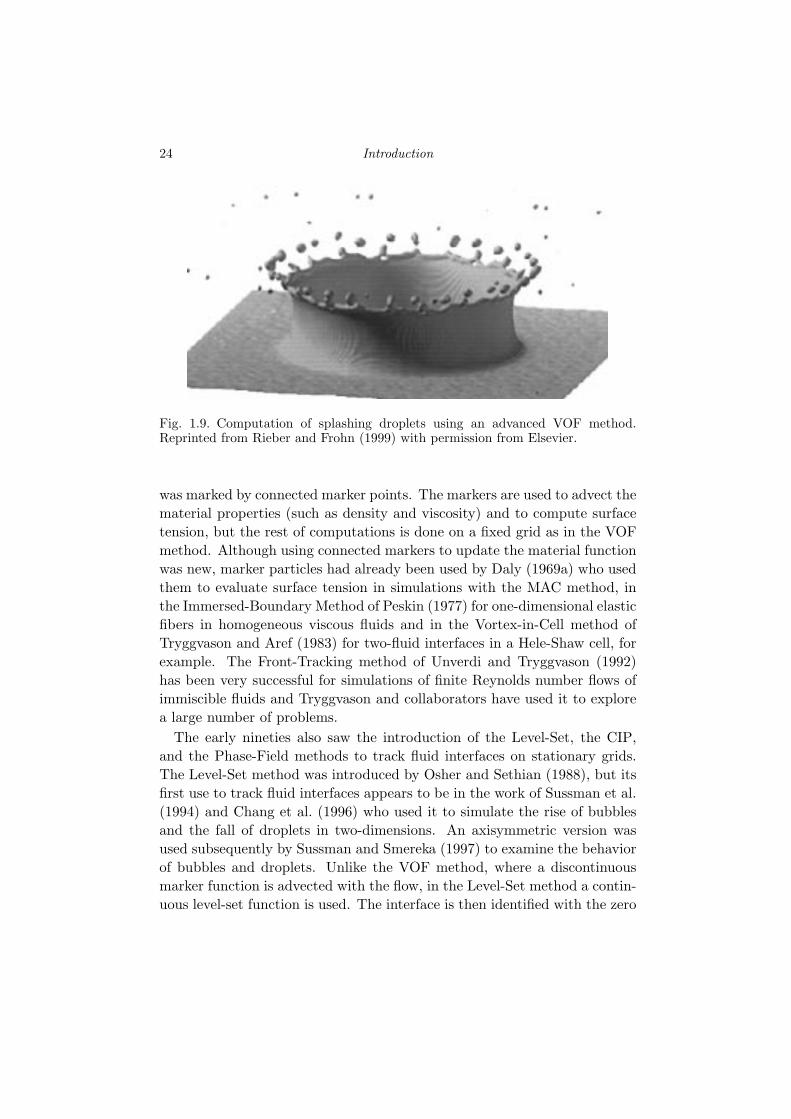
Fig. 1.10. The interaction of two falling spheres. The spheres are shown at fourdifferent times, going from left to right. Reprinted from Hu et al. (2001), withpermission from Elsevier.
move with the fluid velocity, thus deforming the grid. This approach is par-ticularly well-suited when the interface topology is relatively simple and nounexpected interface configurations develop. In a related approach, a gridline is aligned with the fluid interface, but the grid away from the interface isgenerated using standard grid generation techniques such as conformal map-ping or other more advanced elliptic grid generation schemes. The methodwas used by Ryskin and Leal (1984) to compute the steady rise of buoyant,deformable, axisymmetric bubbles. They assumed that the fluid inside thebubble could be neglected, but Dandy and Leal (1989) and Kang and Leal(1987) extended the method to two-fluid problems and unsteady flows. Sev-eral authors have used this approach to examine relatively simple problemssuch as the steady state motion of single particles or moderate deformationof free surfaces. Fully three-dimensional simulations are relatively rare (seethough Takagi et al., 1997) and it is probably fair to say that it is unlikelythat this approach will be the method of choice for very complex problemssuch as the three-dimensional unsteady motion of several particles.
A much more general approach to continuously represent a fluid interfaceby a grid line is to use fully unstructured grids. This allows grid points tobe inserted and deleted as needed and distorted grid cells to be reshaped.While the grid was moved with the fluid velocity in some of the early ap-plications of this method, the more modern approach is to either move onlythe interface points or to move the interior nodes with a velocity differentfrom the fluid velocity, in such a way that the grid distortion is reduced butadequate resolution is still maintained. A large number of methods have

1.3 Looking Ahead 29
been developed that fall into this general category, but we will only refer-ence a few examples. Oran and Boris (1987) simulated the breakup of atwo-dimensional drop; Shopov et al. (1990) examined the initial deforma-tion of a buoyant bubble; Feng et al. (1994), Feng et al. (1995) and Hu(1996) computed the unsteady two-dimensional motion of several particlesand Fukai et al. (1995) followed the collision of a single axisymmetric dropletwith a wall. Although this appears to be a fairly complex approach, Johnsonand Tezduyar (1997) and Hu et al. (2001) have produced very impressive re-sults for the three-dimensional unsteady motion of many spherical particles.Figure 1.10 shows an example of a simulation done using the Arbitrary-Lagrangian-Eulerian method of Hu et al. (2001). Here, two solid spheresare initially falling in-line (left frame). Since the trailing sphere is shelteredfrom the flow by the leading one, it catches up and “kisses” the leading one.The in-line configuration is unstable and the spheres “tumble” (two middleframes). After tumbling the spheres drift apart (right frame).
The most recent addition to the collection of methods to simulate fi-nite Reynolds number multiphase flows is the Lattice-Boltzmann Method(LBM). It is now clear that LBM can be used to obtain results of accuracycomparable to more conventional methods. It is still not clear, however,whether the LBM is significantly faster or simpler than other methods (assometimes claimed), but most likely these methods are here to stay. For adiscussion see, for example, Shan and Chen (1993) and Sankaranarayananet al. (2002). A comparison of results obtained by the LBM method and theFront-Tracking method of Unverdi and Tryggvason (1992) can be found inSankaranarayanan et al. (2003). We will not discuss LBM in this book, butrefer the reader to Rothman and Zaleski (1997) and Chapter 6 in Prosperettiand Tryggvason (2007).
1.3 Looking Ahead
Direct numerical simulations of multiphase flows have come a long way inthe last decade and a half or so. It is now possible to simulate accuratelythe evolution of disperse flows of several hundred bubbles, droplets andparticles for sufficiently long times so that reliable values can be obtained forvarious statistical quantities. Similarly, major progress has been achieved inthe development of methods for more complex flows, including those wherea liquid solidifies or evaporates. Simulations of large systems undergoingboiling and solidification are therefore within reach.
Much remains to be done, however, and it is probably fair to say thatthe use of direct numerical simulations of multiphase flows for research and

30 Introduction
design is still in the embryonic state. The possibility of computing the evo-lution of complex multiphase flows—such as churn-turbulent bubbly flowundergoing boiling, or the breakup of a jet into evaporating droplets—willtransform our understanding of flows of enormous economic significance.Currently, control of most multiphase flow processes is fairly rudimentaryand almost exclusively based on intuition and empirical observations. In-dustries that deal primarily with multiphase flows are, however, multibilliondollar operations and the savings realized if atomizers for spray genera-tion, bubble injectors in bubble columns and inserts into pipes to break updroplets, just to name a few examples, could be improved by just a littlebit would add up to a substantial amount of money. Reliable predictionswould also reduce the design cost significantly for situations such as spacevehicles and habitats where experimental investigations are expensive. And,as the possibilities of manipulating flows at the very smallest scales by eitherstationary or free flowing MEMS devices become more realistic, the need topredict the effect of such manipulations becomes critical.
While speculating about the long term impact of any new technology is adangerous thing—and we will simply state that the impact of direct numer-ical simulations of multiphase flows will without doubt be significant—it iseasier to predict the near future. Apart from the obvious prediction thatcomputers will continue to become faster and more available, we expectthat the development of numerical methods will focus mainly on flows withcomplex physics. Although some progress has already been achieved forflows with variable surface tension, flows coupled to temperature and elec-tric fields and flows with phase change, simulations of such systems are stillfar from being commonplace. In addition to the need to solve a large num-ber of equations, coupled systems generally possess much larger ranges oflength and time scales than simple two-fluid systems. Thus, the incorpo-ration of implicit time-integrators for stiff systems and adaptive griddingwill become even more important. It is also likely, as more and more com-plex problems are dealt with, that the differences between direct numericalsimulations—where everything is resolved fully—and simulations where thesmallest scales are modeled will become blurred. Simulations of atomizationwhere the evolution of thin films are computed by “subgrid” models and verysmall droplets are included as point particles are relatively obvious examplesof such simulations (for a discussion of the point-particle approximation seeChapter 9 in Prosperetti and Tryggvason, 2007, for example). Other exam-ples include possible couplings of continuum approaches as those describedin this Book with microscopic simulations of moving contact lines, kineticseffects at a solidifying interface, and reactions in thin flames. Simulations of

1.3 Looking Ahead 31
non-Newtonian fluids, where the microstructure has to be modeled in sucha way that the molecular structure is accounted for in some way, also fallunder this category.
In addition to the development of more powerful numerical methods, itis increasingly critical to deal with the “human” aspect of large-scale nu-merical simulations. The physical problems that we must deal with and thecomputational tools that are available are rapidly becoming very complex.The difficulty of developing fully parallelized software to solve the continuumequations (fluid flow, mass and heat transfer, etc), where three-dimensionalinterfaces must be handled and the grids must be dynamically adapted, areputting such simulations beyond the reach of a single graduate student. Inthe future these simulations may even be beyond the capacity of small re-search groups. It is becoming very difficult for a graduate student to learneverything that he or she needs to know and make significant new progressin four to five years. Lowering the “knowledge barrier” and ensuring thatnew investigators can enter the field of direct numerical simulations of mul-tiphase flow may well become as important as improving the efficiency andaccuracy of the numerical methods. The present book is an attempt to easethe entry of new researchers into this field.

2
Fluid mechanics with interfaces
The equations governing multiphase flows, where a sharp interface separatesimmiscible fluids or phases, are presented in this Chapter. We first derivethe equations for flows without interfaces, in a relatively standard manner.Then we discuss the mathematical representation of a moving interface andthe appropriate jump conditions needed to couple the equations across theinterfaces. Finally, we introduce the so-called “one-fluid” approach wherethe interface is introduced as a singular distribution in equations writtenfor the whole flow field. The “one-fluid” form of the equations plays afundamental role for the numerical methods discussed in the rest of thebook.
2.1 General principles
The derivation of the governing equations is based on three general prin-ciples: the continuum hypothesis, the hypothesis of sharp interfaces andthe neglect of intermolecular forces. The assumption that fluids can betreated as a continuum is usually an excellent approximation. Real fluidsare, of course, made of atoms or molecules. To understand the continuumhypothesis, consider the density or amount of mass per unit volume. Ifthis amount were measured in a box of sufficiently small dimensions �, itwould be a wildly fluctuating quantity (see Batchelor, 1970, for a detaileddiscussion). However as the box side � increases the density becomes eversmoother, until it is well approximated by a smooth function ρ. For liquidsin ambient conditions this happens for � above a few tens of nanometers (1nm = 10−9 m). In some cases, such as in dilute gases the discrete natureof matter may be felt over much larger length scales. For dilute gases theaverage distance between molecular collisions, or the mean free path �mfp, isthe important length scale. The gas obeys the Navier-Stokes equations for
32

2.2 Basic equations 33
scales �� �mfp. Molecular simulations, where the motion of many individualmolecules is followed for sufficiently long times so that meaningful averagescan be computed, show that the fluid behaves as a continuum for a surpris-ingly small number of molecules. Koplik et al. (1988) found, for example,that under realistic pressure and temperature a few hundred molecules ina channel resulted in a Poiseuille flow that agreed with the predictions ofcontinuum theory.
Beyond the continuum hypothesis, for multiphase flows we shall makethe assumption of sharp interfaces. Interfaces separate different fluids, suchas air and water, oil and vinegar, or any other pair of immiscible fluidsand different thermodynamic phases such as solid and liquid or vapor andliquid. The properties of the fluids, including their equation of state, density,viscosity and heat conductivity, generally change across the interface. Thetransition from one phase to another occurs on very small scales, as describedabove. For continuum scales we may safely assume that interfaces havevanishing thickness.
We also impose certain restrictions on the type of forces that are taken intoaccount. Long range forces between fluid particles, such as electromagneticforces in charged fluids, shall not be considered. Intermolecular forces, suchas Van der Waals forces that play an important role in interface physics, aremodelled by retaining their most important effect: capillarity. This effect,also called surface tension, amounts to a stress concentrated at the sharpinterfaces.
The three assumptions above also reflect the fact that it would be nearlyimpossible, with the current state-of-the-art, to describe complex dropletand bubble interactions while keeping the microscopic physics. For instance,simulating physical phenomena from the nanometer to the centimeter scalewould require 107 grid points in every direction, an extravagant requirementfor any type of computation, even with the use of cleverly employed adaptivemesh refinement.
Beyond the three assumptions above, we mostly deal with incompressibleflows in this Book, although in the present Chapter we derive the equationsinitially for general flow situations.
2.2 Basic equations
Expressing the basic principles of conservation of mass, momentum andenergy mathematically leads to the governing equations for fluid flow. Inaddition to the general conservation principles, we also need constitutive

34 Fluid mechanics with interfaces
n!
ds!
dv! u(x,t)!Volume V!
Surface S!
Fig. 2.1. A stationary control volume V . The surface is denoted by S.
assumptions about the specific nature of each fluid. Here we will work onlywith Newtonian fluids.
2.2.1 Mass conservation
The principle of conservation of mass states that mass cannot be creatednor destroyed. Therefore, if we consider a volume V , fixed in space, thenthe mass inside this volume can only change if mass flows in or out throughits boundary S. The flow out of V , through a surface element ds, is ρu ·ndswhere n is the outward normal, ρ is the density and u is the velocity. Thenotation is shown in Fig. 2.1. Stated in integral form, the principle of massconservation is
d
dt
�
Vρdv = −
�
Sρu · nds. (2.1)
Here, the left hand side is the rate of change of mass in the volume V and theright-hand side represents the net flow through its boundary S. Since thevolume is fixed in space we can take the derivative inside the integral and,by applying the divergence theorem to the integral of the fluxes through theboundary, we have
�
V
�∂ρ
∂t+∇ · (ρu)
�dv = 0. (2.2)
This relation must hold for any arbitrary volume, no matter how small, andthat can only be true if the quantity inside the square brackets is zero. The
2.2 Basic equations 35
partial differential equation expressing conservation of mass is therefore
∂ρ
∂t+∇ · (ρu) = 0. (2.3)
By using the definition of the substantial derivative
D()Dt
=∂()∂t
+ u ·∇(), (2.4)
and expanding the divergence, ∇ · (ρu) = u · ∇ρ + ρ∇ · u, the continuityequation can be rewritten in convective form as
Dρ
Dt= −ρ∇ · u, (2.5)
emphasizing that the density of a material particle can only change if thefluid is compressed or expanded (∇ · u �= 0).
2.2.2 Momentum conservation
The equation of motion is derived by using the momentum-conservationprinciple, stating that the rate of change of fluid momentum in the fixedvolume V is the difference in momentum flux across the boundary S plusthe net forces acting on the volume. Therefore,
d
dt
�
Vρudv = −
�
Sρu(u · n)ds +
�
Vfdv +
�
Sn · Tds. (2.6)
The first term on the right-hand side is the momentum flux through theboundary of V and the next term is the total body force on V . Frequently,the force per unit volume f is only the gravitational force, f = ρg. Thelast term is the total surface force. Here, the tensor T is a symmetric stresstensor constructed in such a way that n·Tds is the force on a surface elementds with a normal n.
By the same argument as applied to the mass conservation equation, equa-tion (2.6) must be valid at every point in the fluid, so that
∂ρu∂t
= −∇ · (ρuu) + f +∇ · T. (2.7)
Here we denote with ab, whose ij-th component is aibj , the dyadic productof the two vectors a and b, hence uu has components uiuj . The nonlinearadvection term can be written as
∇ · (ρuu) = ρu ·∇u + u∇ · (ρu), (2.8)

36 Fluid mechanics with interfaces
and using the definition of the substantial derivative and the continuityequation we can rewrite equation (2.7) as
ρDuDt
= f +∇ · T. (2.9)
This is Cauchy’s equation of motion and is valid for any continuous medium.For fluids like water, oil and air (as well as many others that are generallyreferred to as Newtonian fluids) the stress may be assumed to be a linearfunction of the rate of strain
T = (−p + λ∇ · u)I + 2µS. (2.10)
Here, I is the unit tensor, p the pressure, µ the viscosity and S = 12(∇u +
∇uT ) is the rate-of-strain or deformation tensor whose components are
Sij =12
�∂ui
∂xj+
∂uj
∂xi
�. (2.11)
λ is the second coefficient of viscosity and if Stokes’ hypothesis is assumed tohold, then λ = −(2/3)µ.† Substituting the expression for the stress tensorinto Cauchy’s equation of motion results in
ρDuDt
= f −∇p +∇(λ∇ · u) +∇ · (2µS), (2.12)
which is the Navier-Stokes equation for fluid flow.
2.2.3 Energy conservation
In integral form the conservation of energy principle, as applied to a controlvolume V fixed in space, is:
d
dt
�
Vρ(e +
12u2)dv = (2.13)
−
�
Sρ(e +
12u2)u · nds +
�
Vu · fdv +
�
Sn · (u · T)ds−
�
Sqds.
Here, u2 = u · u and e is the total internal energy per unit mass. Theleft-hand side is the internal and kinetic energy, the first term on the right-hand side is the flow of internal and kinetic energy across the boundary, thesecond term represents the work done by body forces, the third term is thework done by the stresses at the boundary (pressure and viscous shear) andq in the fourth term is the heat-flux vector. This equation can be simplified
† In several texts the discussion is based on the bulk viscosity κ = 2/3µ + λ. Stokes’ hypothesisis that the bulk viscosity vanishes.

2.2 Basic equations 37
by using the momentum equation. Taking the dot product of the velocitywith equation (2.9) gives
ρ∂u2/2
∂t= −ρu ·∇u2/2 + u · f + u · (∇ · T) (2.14)
for the mechanical energy. After using this equation to cancel terms in (2.13)and applying the same arguments as before, we obtain the convective formof the energy equation:
ρDe
Dt−T : ∇u +∇ · q = 0. (2.15)
Here we denote with A : B =�
i
�j AijBji the scalar product of the two
tensors A and B. This equation needs to be supplemented by constitutiveequations for the specific fluids we are considering.
We will assume that the flux of heat is proportional to the gradient of thetemperature T , so that
q = −k∇T. (2.16)
This is called Fourier’s law and k is the thermal conductivity. Using Fourier’slaw, assuming a Newtonian fluid, so that the stress tensor is given by equa-tion (2.10), and that radiative heat transfer is negligible, then the energyequation takes the form:
ρDe
Dt+ p∇ · u = Φ +∇ · k∇T, (2.17)
where Φ = λ(∇ · u)2 + 2µS : S is called the dissipation function. It canbe shown that Φ, which represents the rate at which work is converted intoheat, is always greater or equal to zero.
In general we also need an equation of state giving, say, pressure as afunction of density and internal energy
p = p(e, ρ), (2.18)
as well as equations for the transport coefficients µ, λ and k as functions ofthe state of the fluid.
The governing equations are summarized in Figs. 2.2 to 2.4. The integralform obtained by applying the conservation principles directly to a smallcontrol volume is shown in Fig. 2.2. While usually not very convenient foranalytical work, the integral form is the starting point for Finite-Volumenumerical methods. In Fig. 2.3 we show the differential form obtaineddirectly by assuming that the integral laws hold at a point. This formcan be used for finite difference numerical methods and usually leads to

38 Fluid mechanics with interfaces
d
dt
�
Vρdv +
�
Sρu · nds = 0
d
dt
�
Vρudv =
�
Vfdv +
�
S
�n · T− ρu(u · n)
�ds
d
dt
�
Vρ(e +
12u2)dv =
�
Vu · fdv +
�
Sn · (u · T− ρ(e +
12u2)u− q)ds
Fig. 2.2. The equations of fluid motion in integral form. The flux terms have beenmoved under the same surface integral as the stress terms.
∂ρ
∂t+∇ · (ρu) = 0
∂ρu∂t
= f +∇ · (T− ρuu)
∂
∂tρ(e +
12u2) = −∇ ·
�ρ(e +
12u2)u−T · u + q
�+ u · f
Fig. 2.3. The equations of fluid motion in conservative form.
Dρ
Dt+ ρ∇ · u = 0
ρDuDt
= f +∇ · T
ρDe
Dt= T : ∇u−∇ · q
Fig. 2.4. The equations of fluid motion in convective or non-conservative form.
discretizations that are essentially identical to those obtained by the Finite-Volume method. In Fig. 2.4 we have regrouped the terms to obtain theconvective or the non-conservative form of the equations. This is the formusually shown in textbooks and is often used as a starting point for finitedifference methods.
2.2 Basic equations 39
2.2.4 Incompressible Flow
For an important class of flows the density of each fluid particle does notchange as they move. This is generally the case when the maximum orcharacteristic flow velocity U is much smaller than the velocity of sound cs,or equivalently when the Mach number Ma = U/cs is much smaller thanunity. The equation for the evolution of the density is then
Dρ
Dt=
∂ρ
∂t+ u ·∇ρ = 0, (2.19)
and the mass conservation equation (2.5) becomes
∇ · u = 0. (2.20)
Equation (2.20) states that the volume of any fluid element cannot bechanged and these flows are therefore referred to as incompressible flows.If we integrate this equation over a finite volume V with boundary S anduse the divergence theorem (or expand the divergence in (2.2) and use equa-tion (2.3)), we find that the integral form of the mass conservation equationfor incompressible flows is
�
Su · nds = 0, (2.21)
stating that inflow balances outflow.Notice that there is no requirement that the density is the same every-
where in incompressible flows. The density of a material particle can varyfrom one particle to the next one, but the density of each particle must stayconstant. When the density is not the same everywhere its value at anygiven point in space can change with time as material particles of differentdensity are advected with the flow. In this case the density field must beupdated using equation (2.19). If the density is constant everywhere this is,of course, not necessary.
The pressure plays a special role for incompressible flows. Instead of beinga thermodynamic function of (say) density and temperature, it is determinedsolely by the velocity field and will take on whatever value is necessary tomake the flow divergence free. It is sometimes convenient—and we will usethis extensively—to think of the pressure as projecting the velocity field intothe space of incompressible functions. That is, we imagine the velocity firstbeing predicted by (2.12) without the pressure, then we find the pressurenecessary to enforce incompressibility and correct the velocity field. Noticethat for incompressible flow it is not necessary to solve the energy equa-tion to find the velocity and the pressure, unless the material properties

40 Fluid mechanics with interfaces
∇ · u = 0
ρDuDt
= −∇p + f +∇ · µ(∇u +∇uT )
Fig. 2.5. The equations of fluid motion for incompressible Newtonian flow in con-vective form.
are functions of the temperature. Thus, the flow field is found by solvingthe momentum equation, equation (2.12), along with the incompressibilitycondition, equation (2.20) or (2.21). The governing equations for incom-pressible, Newtonian flows in convective form are summarized in Fig. 2.5.The total derivative in the momentum equation in Fig. 2.5 can be written inseveral different ways, all of which are equivalent analytically but that gener-ally lead to slightly different numerical approximations. The most commonones areDuDt
=∂u∂t
+∇ ·(uu) =∂u∂t
+u ·∇u =∂u∂t
+12∇(u ·u)−u×(∇×u). (2.22)
We will usually work with the second form, but we note that the third oneis very commonly used as well. For compressible flows the fully conservativeform of the momentum equations is usually used, but as discussed at the endof Chapter 3, doing so for incompressible flow with a density that changesabruptly can lead to certain numerical difficulties.
The special case of incompressible fluids with constant density and vis-cosity is of considerable importance. By writing the deformation tensorin component form is easily shown that ∇ · (∇u + ∇uT ) = ∇2u and themomentum equation becomes
∂u∂t
+ u ·∇u−∇p
ρ+
fρ
+ ν∇2u, (2.23)
where ν = µ/ρ is the kinematic viscosity.
2.2.5 Boundary conditions
One of the major difficulties in numerical simulations of fluid flows is thecorrect implementation of the boundary conditions. In principle the condi-tions at boundaries are well defined. For viscous, incompressible fluids werequire the fluid to stick to the wall so the fluid velocity there is equal tothe wall velocity
u = Uwall. (2.24)

2.2 Basic equations 41
n
solidβ
Fig. 2.6. In some models the fluid is allowed to slip on the solid surface. Thevelocity vanishes at some distance β inside the solid, called the slip length. Thismodel is useful when dealing with triple lines (contact lines) involving two fluidsand a solid.
This equation includes both the normal and the tangential components ofthe velocity. For inviscid flows, where viscous stresses are absent and thefluid can slip freely at the wall, only the normal velocity is equal to thatof the wall. In some cases, for instance for flow in very small channels, itis useful to introduce a slip boundary condition for the tangential velocitycomponent ut
ut − Uwall = β∂ut
∂n. (2.25)
Here β is a slip coefficient, with the dimensions of a (small) length and ∂/∂nis the derivative in the direction normal to the wall. The slip length is thedistance at which the velocity would vanish if extrapolated inside the wall(Fig. 2.6).
Frequently we are interested in simulating a fluid domain with in- andoutflow boundaries, or we are interested in simulating only a part of a largerfluid-filled domain. In those cases it is necessary to specify in- and outflowboundary conditions. For inflow boundaries the velocity is usually given.Realistic outflow boundaries, on the other hand, pose a challenge that un-fortunately does not have a simple solution. Similar difficulties are facedby the experimentalist who must carefully design his or her wind tunnelto provide uniform inlet velocity and outlet conditions that have minimalinfluence on the upstream flow. While it is probably easier to implement uni-form inlet conditions computationally than in experiments, the outlet flowis more problematic since the solution often available to the experimentalist,simply by making the wind tunnel long enough, usually requires extensivenumber of grid points. The goal is generally to truncate the domain using
42 Fluid mechanics with interfaces
h(x,t)
y
x
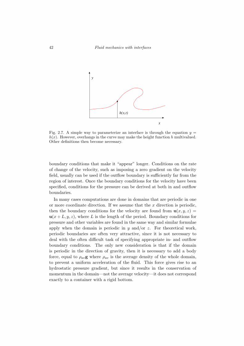
Fig. 2.7. A simple way to parameterize an interface is through the equation y =h(x). However, overhangs in the curve may make the height function h multivalued.Other definitions then become necessary.
boundary conditions that make it “appear” longer. Conditions on the rateof change of the velocity, such as imposing a zero gradient on the velocityfield, usually can be used if the outflow boundary is sufficiently far from theregion of interest. Once the boundary conditions for the velocity have beenspecified, conditions for the pressure can be derived at both in and outflowboundaries.
In many cases computations are done in domains that are periodic in oneor more coordinate direction. If we assume that the x direction is periodic,then the boundary conditions for the velocity are found from u(x, y, z) =u(x + L, y, z), where L is the length of the period. Boundary conditions forpressure and other variables are found in the same way and similar formulaeapply when the domain is periodic in y and/or z. For theoretical work,periodic boundaries are often very attractive, since it is not necessary todeal with the often difficult task of specifying appropriate in- and outflowboundary conditions. The only new consideration is that if the domainis periodic in the direction of gravity, then it is necessary to add a bodyforce, equal to ρavg where ρav is the average density of the whole domain,to prevent a uniform acceleration of the fluid. This force gives rise to anhydrostatic pressure gradient, but since it results in the conservation ofmomentum in the domain—not the average velocity—it does not correspondexactly to a container with a rigid bottom.

2.3 Interfaces: description and definitions 43
Fluid 2
tFluid 1
un
x(u)=(x(u),y(u))x
y
Fig. 2.8. A parameterization of the interface. The coordinate u follows the interface.
2.3 Interfaces: description and definitions
Following the motion of a deformable interface separating different fluids orphases is at the center of accurate predictions of multiphase flows. Describ-ing the interface location and how it moves can be accomplished in severalways. The simplest case is when the location of the interface can be de-scribed by a single-valued function of one (in two dimensions) or two (inthree dimensions) coordinates. For a thin liquid layer, we can, for example,write
y = h(x) (two dimensions); z = h(x, y) (three dimensions). (2.26)
This situation is sketched in Fig. 2.7, which also shows the limitation of thisapproach: if part of the interface “overhangs,” h becomes a multi-valuedfunction. While there are many situations, particularly for thin films, whereequation (2.26) is the most convenient description, generally we need a moresophisticated way to describe the interface.
To handle interfaces of arbitrary shape we can parameterize the interfaceby introducing a coordinate u in two dimensions, such that the location ofthe interface is given by
x(u) =�x(u), y(u)
�. (2.27)
Fig. 2.8 shows a closed contour separating fluid “1” from fluid “2”, de-scribed in this way. For a curve in two dimensions, described by equation(2.27), dx/du yields a vector tangent to the curve. Although u can be any
44 Fluid mechanics with interfaces
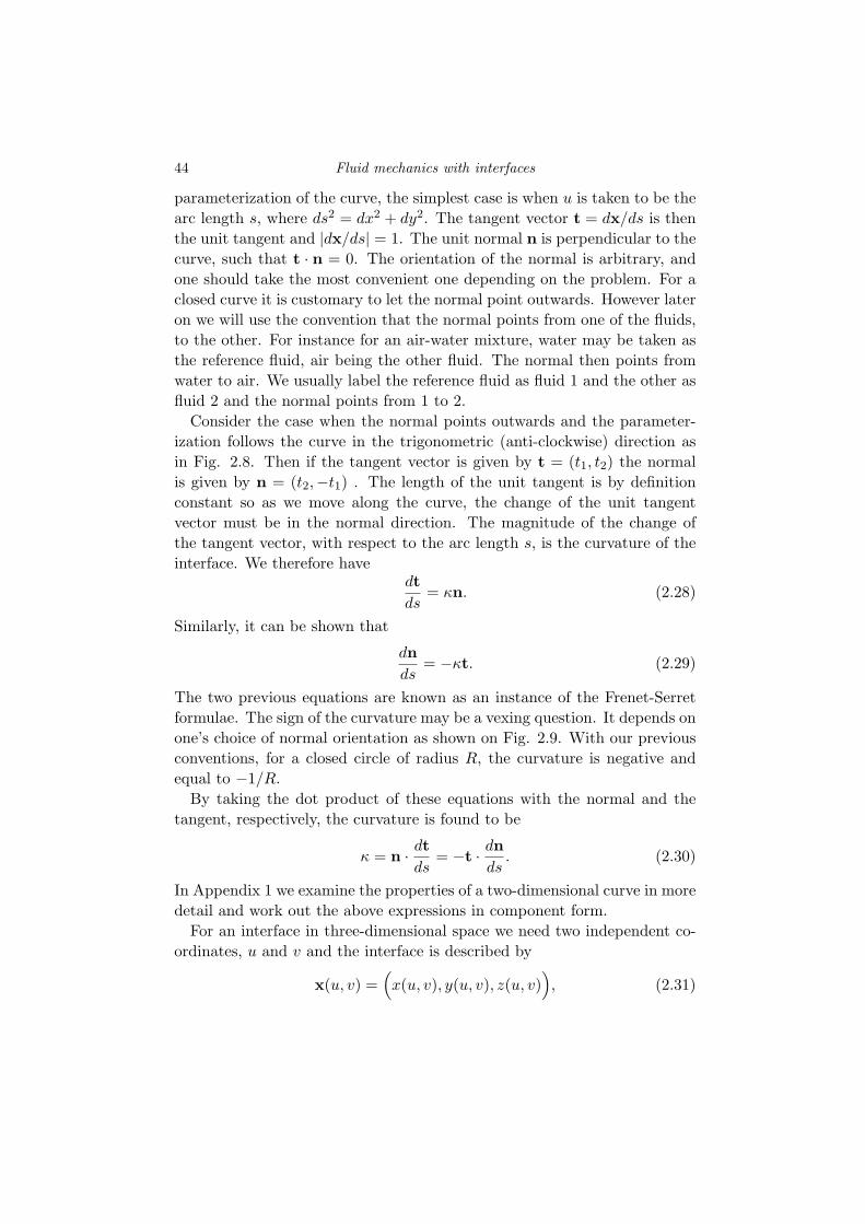
parameterization of the curve, the simplest case is when u is taken to be thearc length s, where ds2 = dx2 + dy2. The tangent vector t = dx/ds is thenthe unit tangent and |dx/ds| = 1. The unit normal n is perpendicular to thecurve, such that t · n = 0. The orientation of the normal is arbitrary, andone should take the most convenient one depending on the problem. For aclosed curve it is customary to let the normal point outwards. However lateron we will use the convention that the normal points from one of the fluids,to the other. For instance for an air-water mixture, water may be taken asthe reference fluid, air being the other fluid. The normal then points fromwater to air. We usually label the reference fluid as fluid 1 and the other asfluid 2 and the normal points from 1 to 2.
Consider the case when the normal points outwards and the parameter-ization follows the curve in the trigonometric (anti-clockwise) direction asin Fig. 2.8. Then if the tangent vector is given by t = (t1, t2) the normalis given by n = (t2,−t1) . The length of the unit tangent is by definitionconstant so as we move along the curve, the change of the unit tangentvector must be in the normal direction. The magnitude of the change ofthe tangent vector, with respect to the arc length s, is the curvature of theinterface. We therefore have
dtds
= κn. (2.28)
Similarly, it can be shown that
dnds
= −κt. (2.29)
The two previous equations are known as an instance of the Frenet-Serretformulae. The sign of the curvature may be a vexing question. It depends onone’s choice of normal orientation as shown on Fig. 2.9. With our previousconventions, for a closed circle of radius R, the curvature is negative andequal to −1/R.
By taking the dot product of these equations with the normal and thetangent, respectively, the curvature is found to be
κ = n ·dtds
= −t ·dnds
. (2.30)
In Appendix 1 we examine the properties of a two-dimensional curve in moredetail and work out the above expressions in component form.
For an interface in three-dimensional space we need two independent co-ordinates, u and v and the interface is described by
x(u, v) =�x(u, v), y(u, v), z(u, v)
�, (2.31)

2.3 Interfaces: description and definitions 45
Fig. 2.9. The sign of the curvature depends on one’s choice for the orientation ofthe normal. If the curve folds towards the normal the curvature is positive.
xun
xvA
p
t
v=constx(u,v)=(x(u,v), y(u,v), z(u,v))
u=const
Fig. 2.10. A small surface element. The surface is parameterized by u and v. p isa vector perpendicular to the edge of the element but tangent to the surface.
as shown in Fig. 2.10. The geometry of three-dimensional surfaces is anelaborate subject and we will only need a few specific results. To avoidcluttering the discussion unnecessarily we have gathered some of the morepertinent elements of the theory in Appendix 1 and here we simply quotethe results that we need.
In addition to knowing the location of the interface, we frequently needto compute the normal to the interface, tangent vectors and the mean cur-vature. Differentiating x(u, v) with respect to the surface coordinates yields
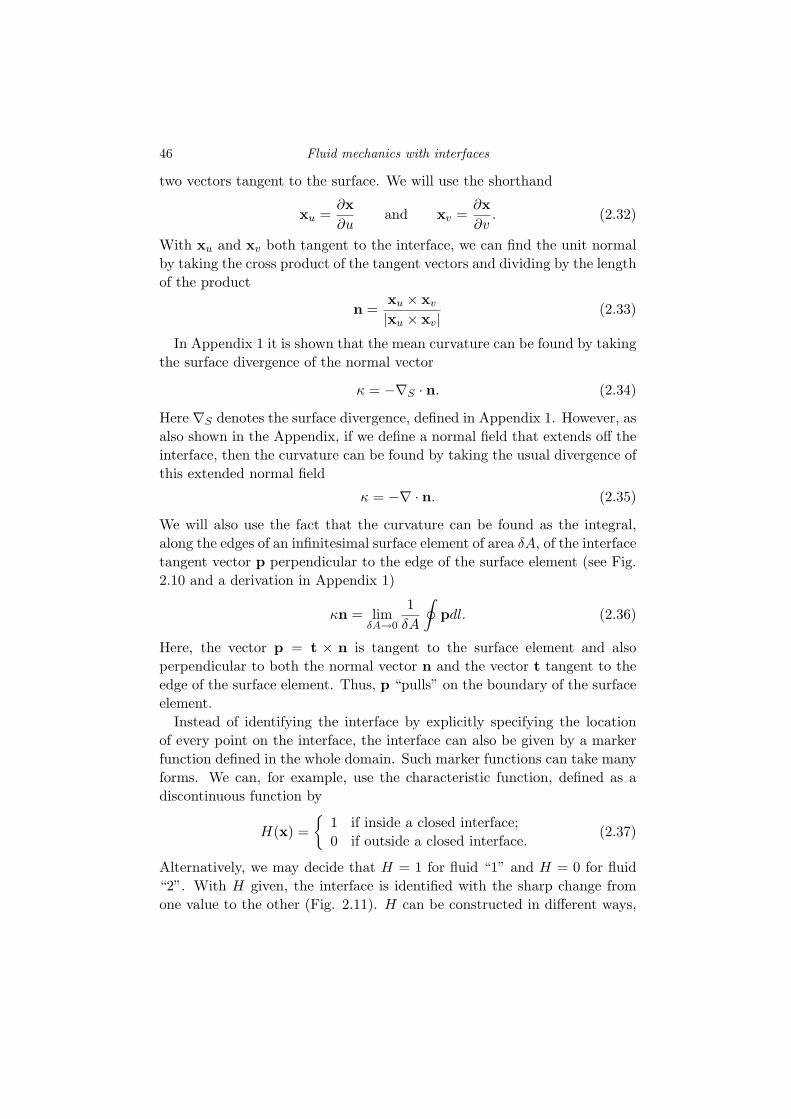
46 Fluid mechanics with interfaces
two vectors tangent to the surface. We will use the shorthand
xu =∂x∂u
and xv =∂x∂v
. (2.32)
With xu and xv both tangent to the interface, we can find the unit normalby taking the cross product of the tangent vectors and dividing by the lengthof the product
n =xu × xv
|xu × xv|(2.33)
In Appendix 1 it is shown that the mean curvature can be found by takingthe surface divergence of the normal vector
κ = −∇S · n. (2.34)
Here ∇S denotes the surface divergence, defined in Appendix 1. However, asalso shown in the Appendix, if we define a normal field that extends off theinterface, then the curvature can be found by taking the usual divergence ofthis extended normal field
κ = −∇ · n. (2.35)
We will also use the fact that the curvature can be found as the integral,along the edges of an infinitesimal surface element of area δA, of the interfacetangent vector p perpendicular to the edge of the surface element (see Fig.2.10 and a derivation in Appendix 1)
κn = limδA→0
1δA
�pdl. (2.36)
Here, the vector p = t × n is tangent to the surface element and alsoperpendicular to both the normal vector n and the vector t tangent to theedge of the surface element. Thus, p “pulls” on the boundary of the surfaceelement.
Instead of identifying the interface by explicitly specifying the locationof every point on the interface, the interface can also be given by a markerfunction defined in the whole domain. Such marker functions can take manyforms. We can, for example, use the characteristic function, defined as adiscontinuous function by
H(x) =�
1 if inside a closed interface;0 if outside a closed interface.
(2.37)
Alternatively, we may decide that H = 1 for fluid “1” and H = 0 for fluid“2”. With H given, the interface is identified with the sharp change fromone value to the other (Fig. 2.11). H can be constructed in different ways,

2.3 Interfaces: description and definitions 47
H=1!
H=0!
dv’=dx’dy’!
S!
x!
y!
V!
ds’!
Fig. 2.11. A step function identifying the region occupied by a specific fluid.
but for our purpose it is convenient to express it in terms of an integral overthe product of one-dimensional δ-functions. For a two-dimensional domain:
H(x, y) =�
Vδ(x− x�)δ(y − y�)dv�. (2.38)
Here, the integration is over the region bounded by the contour S and dv� =dx�dy� (Fig. 2.11). Obviously, H = 1 if the point (x, y) is inside the contour,where it will coincide with (x�, y�) during the integration, and zero if it isoutside and will never be equal to (x�, y�) .
The properties of the step function are discussed in more detail in Ap-pendix 1 where we show that the gradient of H is given by
∇H(x, y) = −�
Sδ(x− x�)δ(y − y�)n�ds� = −δ(n)n, (2.39)
where n is the coordinate normal to the interface in a local coordinate systemaligned with the interface. We can also define a surface distribution δS(x) =δ(n), and write
∇H = −δSn. (2.40)
In addition, the interface can be described by a smooth function F , if theinterface is identified with a particular value of the function, say F = 0 (Fig.2.12). Obviously, F < 0 on one side of the interface and F > 0 on the other.One usually takes the reference fluid (fluid “1”) to be in the F > 0 region.Taking F > 0 inside the closed surface, the normal points outwards and is

48 Fluid mechanics with interfaces
Fig. 2.12. The identification of an interface by a level-set function.
found by
n = −∇F
|∇F |(2.41)
and the curvature is given by
κ = −∇ · n = ∇ ·
�∇F
|∇F |
�. (2.42)
The representation of the interface as a contour with a specific value is usedin Level-Set methods.
The motion of the interface S is determined by the normal velocity V (u, v, t),for each point on S. This velocity may be that of the fluid itself, or may bedifferent due to, for example, evaporation or condensation. In parametricform
V (u, v, t) = n ·∂
∂tx(u, v, t). (2.43)
To update the location of S, we note that there is no need to specify atangential velocity, although from a physical point of view the interface is

2.4 Fluid mechanics with interfaces 49
n V
u2
u1
S
V
S
Fig. 2.13. A thin control volume δV with boundary δS including a portion of theinterface S. The thickness of the control volume is taken to be zero, so no accumu-lation takes place.
made of fluid particles that travel at some tangential as well as normalvelocity. The fact that the motion of the interface is determined only by thenormal velocity at the interface can be seen by considering the interface asa level-set function F . Since the function moves with the fluid velocity, itsmotion is described by
DF
Dt=
∂F
∂t+ u ·∇F = 0. (2.44)
The normal to the interface is given by (2.41) so we can rewrite the aboveequation as
∂F
∂t− u · n|∇F | =
∂F
∂t− V |∇F | = 0. (2.45)
which involves only the normal velocity V = u · n.
2.4 Fluid mechanics with interfaces
Consider the incompressible flow of two immiscible fluids filling a given do-main. The domain may be decomposed into any number of subdomains filledwith the individual phases. In any subdomain the usual Navier-Stokes equa-tions hold and here we derive the interface conditions that allow us to couplethe fluid motion in the different fluids, across the interface. These conditionsare, for the most part, derived using mass and momentum conservation. Inone case (for surface tension) it is necessary to introduce additional physics.

50 Fluid mechanics with interfaces
2.4.1 Mass conservation and velocity conditions
To derive the jump conditions for the normal velocity, we apply the conser-vation principle used in Section 2.2.1 to the control volume shown in Fig.2.13. Since its thickness is taken to be zero, there can be no accumulationof mass inside it, so the mass flux into the control volume must be equal tothe flow out. If the velocity on one side of the interface is u1 and on theother it is u2 and the normal velocity of the interface is V , then the inflowis u1 · n − V and the outflow is u2 · n − V . Denoting the mass flow acrossthe interface by m, we have
ρ1(u1 · n− V ) = ρ2(u2 · n− V ) = m . (2.46)
This is simply the Rankine-Hugoniot condition. If there is no change ofphase, m = 0. For incompressible flows this condition must hold for arbi-trary density ratios and we therefore have
V = u1 · n = u2 · n. (2.47)
Mass conservation places no restriction on the tangential velocity compo-nents. Indeed, inviscid fluids are usually assumed to slip at the interface.For very low viscosity and rarefied gases it is possible that finite slip is theappropriate interface condition, but for viscous fluid under normal operatingconditions it is an experimentally observed fact—like the no-slip boundaryconditions at solid walls—that no slip takes place. It is also possible to arguethat if the sharp interface is assumed to come about by taking the limit of afinite interface zone as its thickness goes to zero, then anything but no slipwould result in infinitely high stresses if the interface zone consists of a fluidwith a finite viscosity. Thus, if there is no phase change and the fluids areincompressible, the interfacial condition for viscous fluid is simply u1 = u2,or
[u]S = 0, (2.48)
where we have used the jump notation, i. e. the notation [x]S = x2 − x1.
2.4.2 Surface tension
From a molecular point of view, surface tension arises because the interfaceis not an optimal region thermodynamically: the molecules “prefer” to beat the gas or the liquid density, which minimizes the free energy. The non-optimal conditions near the interface result in an excess energy
dEσ = σds, (2.49)
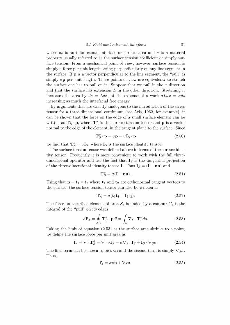
2.4 Fluid mechanics with interfaces 51
where ds is an infinitesimal interface or surface area and σ is a materialproperty usually referred to as the surface tension coefficient or simply sur-face tension. From a mechanical point of view, however, surface tension issimply a force per unit length acting perpendicularly on any line segment inthe surface. If p is a vector perpendicular to the line segment, the “pull” issimply σp per unit length. These points of view are equivalent: to stretchthe surface one has to pull on it. Suppose that we pull in the x directionand that the surface has extension L in the other direction. Stretching itincreases the area by ds = Ldx, at the expense of a work σLdx = σdsincreasing as much the interfacial free energy.
By arguments that are exactly analogous to the introduction of the stresstensor for a three-dimensional continuum (see Aris, 1962, for example), itcan be shown that the force on the edge of a small surface element can bewritten as Tσ
S · p, where TσS is the surface tension tensor and p is a vector
normal to the edge of the element, in the tangent plane to the surface. Since
TσS · p = σp = σIS · p (2.50)
we find that TσS = σIS , where IS is the surface identity tensor.
The surface tension tensor was defined above in terms of the surface iden-tity tensor. Frequently it is more convenient to work with the full three-dimensional operator and use the fact that IS is the tangential projectionof the three-dimensional identity tensor I. Thus IS = (I− nn) and
TσS = σ(I− nn). (2.51)
Using that n = t1 × t2 where t1 and t2 are orthonormal tangent vectors tothe surface, the surface tension tensor can also be written as
TσS = σ(t1t1 + t2t2). (2.52)
The force on a surface element of area S, bounded by a contour C, is theintegral of the “pull” on its edges
δFσ =�
CTσ
S · pdl =�
S∇S · Tσ
Sds. (2.53)
Taking the limit of equation (2.53) as the surface area shrinks to a point,we define the surface force per unit area as
fσ = ∇ · TσS = ∇ · σIS = σ∇S · IS + IS ·∇Sσ. (2.54)
The first term can be shown to be σκn and the second term is simply ∇Sσ.Thus,
fσ = σκn +∇Sσ, (2.55)

52 Fluid mechanics with interfaces
where the last term, the surface gradient of σ, is obviously zero for constantsurface tension.
2.4.3 Momentum conservation with interfaces
Applying the conservation of momentum principle to the control volume inFig. 2.13, moving with the interface S, we obtain
0 = −�
δSρu(u · n− V )ds +
�
δSn · Tds +
�
Sfσds, (2.56)
Notice that the integration is around the edges of the control volume δVfor the first two terms and along the interface for the last term. The firstterm on the right-hand side is zero for incompressible flows in the absence ofphase change, since the control volume is moving with the fluid velocity. Asthe thickness of the control volume approaches zero, the boundary coincideswith the interface and by integrating the stresses first on one side and thenon the other, the second term yields the jump in T across the interface.Since the results hold for any control volume that includes the interface,they must be valid at any interface point, resulting in
− [T]S · n = σκn +∇Sσ. (2.57)
This condition may be split into a normal and tangential stress condition,using equation (2.55) for fσ, yielding the boxed jump conditions in Fig. 2.14.
2.4.4 Free-surface flow
Free-surface flow is a limiting case of flows with interfaces, in which thetreatment of one of the fluids is simplified. For air-water flow, for instance,we can sometimes assume that the pressure pfree in the air is a constant, ordepends only on time, and that the viscous stresses in the air are negligible.The jump conditions then become boundary conditions for the liquid domainas shown in Fig. 2.15. In the case of constant σ, the tangential stressesvanish and
t(k)· S · n
���S
= 0. (2.58)
This is a purely kinematic condition: it does not involve material propertiesat all. For this reason it has interesting consequences. The vorticity vectoris defined in general as ∇×u and its study reveals interesting aspects of the

2.4 Fluid mechanics with interfaces 53
[u]S = 0,
− [−p + 2µn · S · n]S = σκ,
−
�2µt(k)
· S · n�
S= t(k)
·∇Sσ,
∇ · u = 0,
ρDuDt
= −∇p + f + µ∇2u.
Fig. 2.14. The jump conditions and the partial differential equations for a New-tonian, incompressible fluid, without evaporation or condensation. The last twoequations apply in the bulk of each phase. The first three are jump conditions onthe interface S. There, the t(k) are two unit tangent vectors. In the two-dimensionalflow case there is a single tangent vector. Together with boundary conditions onwalls or entry and exit conditions, these equations form a complete set for flowswith interfaces.
(−p + 2µn · S · n)|S = −pfree + σκ,
2µ t(k)· S · n
���S
= t(k)·∇Sσ,
∇ · u = 0,
ρDuDt
= −∇p + f + µ∇2u.
Fig. 2.15. The boundary conditions and the partial differential equations for aNewtonian, incompressible fluid with a free surface. In this example the pressureon the free surface is set to pfree.
dynamics of the flow. In two dimensions, we note ω = (∇× u) · ez its onlynon-zero component. Then on the free surface
ω = 2κq (2.59)
where q = (u · u)1/2 is the norm of the velocity as shown in Batchelor(1970). This implies that a large vorticity will be seen on the free surface inregions of high velocity and high curvature. This is were the departure fromthe hypothesis of irrotational flow will be the most pronounced. Moreover,the vorticity is also seen in these regions for two-phase flows with a strongdensity and viscosity contrast, since these flows resemble free-surface flows.

54 Fluid mechanics with interfaces
Numerical simulations show characteristic patches of vorticity in the regionsof high curvature.
2.5 Fluid mechanics with interfaces: the one-fluid formulation
In contrast to the approach described in Section 2.4, where we wrote thegoverning equations separately for each phase and used jump conditions tocouple the solutions at the fluid interface, it is possible to write one setof governing equations for the whole flow domain occupied by the variousphases, without resorting to jump conditions. The various phases are treatedas one fluid with variable material properties that change abruptly at thephase boundary. To account for the “extra” forces at the phase boundary itis, however, necessary to add singular terms (δ-functions) to the equations.These singular terms are the counterpart of the jump conditions of the pre-ceding section and it can be shown that both formulations are equivalent.
This form of the equations is often referred to as the “one-fluid” approach.Since the solution can change discontinuously across the interface, we musteither interpret the governing equations in a weak sense where they aresatisfied only in an integral sense, or admit solutions that include generalizedfunctions such as delta functions and step functions. The latter approachis taken here. The “one-fluid” formulation is the starting point for severalnumerical methods based on the use of fixed grids, as we will see in laterChapters.
The derivation of the “one-fluid” equations is exactly the same as before(Section 2.2) except that we need to add the surface tension as a body forceto the momentum equation. The mass conservation equation for the totalmass has no source terms. For reacting flows the conservation equation foreach species may have localized source terms and for flows with phase change(Chapter 11) we shall see that a localized volume source emerges naturallyat the phase boundary.
For a control volume including an interface, the surface tension force isgiven by fσ integrated over S, the part of the surface enclosed in the controlvolume. Just as we use the divergence theorem to convert surface integralsto volume integrals, we use equation (A2.9) to transform the surface integral
�
Sfσds =
�
VfσδSdv, (2.60)
where δS = δS(x−xs). Adding this force to the integral form of the momen-tum equation, equation (2.6), and applying the same arguments as before—that the integral can only be zero for all possible control volumes if the

2.6 Nondimensional numbers 55
integrand is zero—we obtain the “one-fluid” version of the Navier-Stokesequation for incompressible, Newtonian flows with sharp interfaces
ρ∂u∂t
+ ρ∇ · uu = −∇p + f +∇ · µ[∇u + (∇u)T ] + fσδS . (2.61)
We emphasize that this equation holds for the whole flow field, even if thedensity field ρ and the viscosity field µ change discontinuously. For constantsurface tension, the surface force is
fσδS = σκnδS . (2.62)
For completeness we observe that the last term can be written in severaldifferent, but equivalent forms:
fσδS =�
fσδ(x− xs)dA and σκnδS =�
σκnδ(x− xs)dA, (2.63)
where we have used that δ(x − xs) = δ(x − xs)δ(y − ys)δ(z − zs). Noticealso that it is possible to add an arbitrary constant to the surface tensionterm, replacing σκ by (σκ + ∆po). The constant ∆po is balanced exactlyby a change in the pressure jump across the interface and since the flowon either side of the interface is driven by the pressure gradient—not theabsolute value of the pressure—adding the constant has no effect on the flow.Jan (1994) used this observation to subtract the average pressure inside abubble to reduce the pressure jump across the interface in his computationsof the motion of clean and contaminated axisymmetric and two-dimensionalbubbles.
2.6 Nondimensional numbers
The dynamics of multifluid and multiphase flows is governed by a varietyof nondimensional numbers, depending on the exact situation driving theflow. Those include the Reynolds number Re, usually defined based on theproperties of one of the fluids, using an external length scale L and velocityU
Re =ρLU
µ=
LU
ν. (2.64)
Re represents the ratio of inertial to viscous forces. If we construct a velocityscale by
�(∆ρ/ρ)gL, then the square of the Reynolds number becomes the
Galileo number
N =gρ∆ρL3
µ2. (2.65)

56 Fluid mechanics with interfaces
The ratio of inertia to surface tension gives the Weber number defined by
We =ρLU2
σ, (2.66)
and the ratio of viscous to capillary stresses yields the capillary number givenby
Ca =µU
σ. (2.67)
Eliminating the velocity U between the Reynolds and Weber numbers givesthe Ohnesorge number
Oh =µ
√ρσL
. (2.68)
We sometimes also work with the Laplace number, defined by La = 1/Oh2.The combination
Eo =∆ρgL2
σ, (2.69)
defines the Eotvos number, sometimes also called the Bond number. TheMorton number is given by
Mo =∆ρgµ4
ρ2σ3. (2.70)
The Morton number has the attractive property that for a given g, it dependsonly on the fluid properties. When inertia and gravity are the importantforces, such as for surface waves, we often work with the Froude number
Fr =U2
gL. (2.71)
The numbers listed here are the most common ones for two-fluid flows. Forsystems with more complex physics, such as heat or mass transfer, phasechange and chemical reactions, additional numbers must be defined.
2.7 Thin films, intermolecular forces and contact linesTopology changes in multiphase flows, such as when two droplets coalesceinto one or one droplet breaks into two, take place when thin films rup-ture and thin threads snap. Thin threads appear to be—by far—the easiestto deal with. There are good reasons to believe that the Navier-Stokesequations describe how their diameter becomes zero in a finite time andsimulations suggest that the overall results are relatively insensitive to howthey are treated. For thin films, on the other hand, it is necessary to include
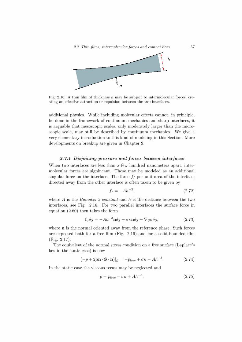
2.7 Thin films, intermolecular forces and contact lines 57
Fig. 2.16. A thin film of thickness h may be subject to intermolecular forces, cre-ating an effective attraction or repulsion between the two interfaces.
additional physics. While including molecular effects cannot, in principle,be done in the framework of continuum mechanics and sharp interfaces, itis arguable that mesoscopic scales, only moderately larger than the micro-scopic scale, may still be described by continuum mechanics. We give avery elementary introduction to this kind of modeling in this Section. Moredevelopments on breakup are given in Chapter 9.
2.7.1 Disjoining pressure and forces between interfaces
When two interfaces are less than a few hundred nanometers apart, inter-molecular forces are significant. Those may be modeled as an additionalsingular force on the interface. The force fI per unit area of the interface,directed away from the other interface is often taken to be given by
fI = −Ah−3, (2.72)
where A is the Hamaker’s constant and h is the distance between the twointerfaces, see Fig. 2.16. For two parallel interfaces the surface force inequation (2.60) then takes the form
fσδS = −Ah−3nδS + σκnδS +∇SσδS , (2.73)
where n is the normal oriented away from the reference phase. Such forcesare expected both for a free film (Fig. 2.16) and for a solid-bounded film(Fig. 2.17).
The equivalent of the normal stress condition on a free surface (Laplace’slaw in the static case) is now
(−p + 2µn · S · n)|S = −pfree + σκ−Ah−3. (2.74)
In the static case the viscous terms may be neglected and
p = pfree − σκ + Ah−3, (2.75)

58 Fluid mechanics with interfaces
P (h)
Fig. 2.17. A film near a solid wall. Positive disjoining pressure will result in thefilm being broken.
so the pressure is increased or decreased depending on the sign of A. ThusΠ(h) = −Ah−3 is called the disjoining pressure. When A > 0 the disjoiningpressure is negative and the interfaces attract each other. On the otherhand when A < 0 the disjoining pressure is positive and the interfaces repeleach other. The value of A depends on the fluid but values in the rangeof 10−20 Joules are common. It is well known that when A > 0 the filmbreaks, as for pure water, while when A < 0 the film is stable, as for watercontaminated with surfactants. Indeed positive A tends to increase thepressure in narrow regions and forces the fluid to flow out of them. Thus acatastrophic instability occurs and the film ruptures.
In principle, equation (2.74) can be used when solving the Navier-Stokesequation for the macroscopic flow evolution. However, the range of scalesthat must be resolved is enormous and this has seldom been achieved in theliterature.
2.7.2 Contact line statics and dynamics
The interface separating two fluids may meet a solid boundary at a contactline (Fig. 2.18). In the absence of motion, the contact line angle θ is fixedby the capillary properties of the substrate and the two fluids. Considera liquid and a gas on a solid surface. The liquid-gas surface energy perunit area is the capillary tension σ. For the liquid-solid and the gas-solidinterfaces we have respectively energies per unit area σls and σgs. Movingthe contact point by a small distance δx along the solid surface results in again of energy σgsδx on one side and a loss (σls + σ cos θeq)δx on the otherside. Equating these energies yields the famous Young-Laplace relation
σgs = σls + σ cos θeq, (2.76)
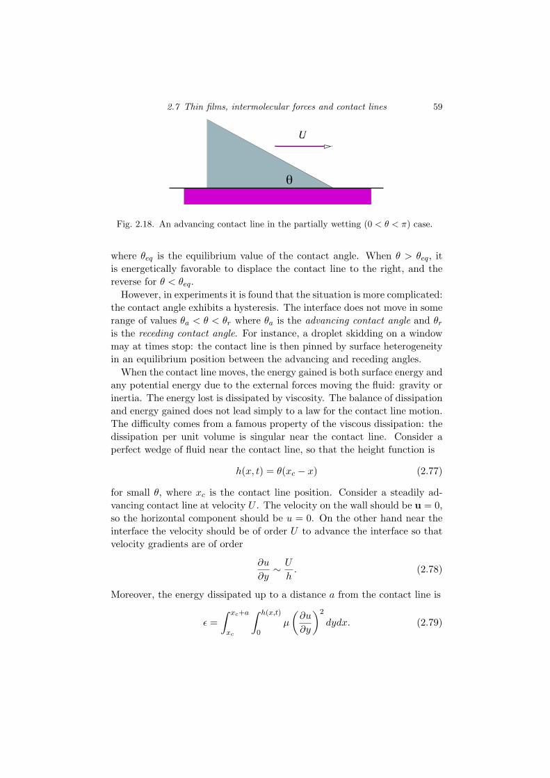
2.7 Thin films, intermolecular forces and contact lines 59
U
θ
Fig. 2.18. An advancing contact line in the partially wetting (0 < θ < π) case.
where θeq is the equilibrium value of the contact angle. When θ > θeq, itis energetically favorable to displace the contact line to the right, and thereverse for θ < θeq.
However, in experiments it is found that the situation is more complicated:the contact angle exhibits a hysteresis. The interface does not move in somerange of values θa < θ < θr where θa is the advancing contact angle and θr
is the receding contact angle. For instance, a droplet skidding on a windowmay at times stop: the contact line is then pinned by surface heterogeneityin an equilibrium position between the advancing and receding angles.
When the contact line moves, the energy gained is both surface energy andany potential energy due to the external forces moving the fluid: gravity orinertia. The energy lost is dissipated by viscosity. The balance of dissipationand energy gained does not lead simply to a law for the contact line motion.The difficulty comes from a famous property of the viscous dissipation: thedissipation per unit volume is singular near the contact line. Consider aperfect wedge of fluid near the contact line, so that the height function is
h(x, t) = θ(xc − x) (2.77)
for small θ, where xc is the contact line position. Consider a steadily ad-vancing contact line at velocity U . The velocity on the wall should be u = 0,so the horizontal component should be u = 0. On the other hand near theinterface the velocity should be of order U to advance the interface so thatvelocity gradients are of order
∂u
∂y∼
U
h. (2.78)
Moreover, the energy dissipated up to a distance a from the contact line is
� =� xc+a
xc
� h(x,t)
0µ
�∂u
∂y
�2
dydx. (2.79)

60 Fluid mechanics with interfaces
Using (2.77) and the estimate (2.78) for the velocity gradient this becomes
� =� a
0µ
U2
θxdx (2.80)
which diverges logarithmically near x = 0. This divergence leads to a para-dox: in the framework of continuum mechanics any motion of the contactline would dissipate infinite energy and thus the contact line cannot move.One way out of the paradox is to use partial-slip boundary conditions suchas equation (2.25). This cuts off the divergence and the dissipation becomes
� =µU2
θln
�a
β
�. (2.81)
2.8 Notes2.8.1 Fluid and interface mechanics
A derivation or even a textbook presentation of the equations governingfluid interfaces is not the primary purpose of this monograph. The inter-ested reader may consult basic fluid mechanics treatises such as Batchelor(1970) who devotes ample space to issues involving interfaces and for a moresystematic description of interface geometry the reader is referred to Weath-erburn (1927) as well as other references, such as Aris (1962).
While the constitutive assumption given by equation (2.49) allows forvariable surface tension, due to contaminants or temperature variations, forexample, we have excluded any stresses due to surface shear or dilation.More complex constitutive equations can be introduced to account for sucheffects, see Scriven (1960), Aris (1962) and Edwards et al. (1961) for discus-sions.
2.8.2 Thin films and contact lines
Intermolecular forces, our equation (2.72), can be modeled in a variety ofways, depending on the polar nature of the interface, on electric chargesand the presence of large molecules on the interface. Other forms of thedisjoining pressure may be found in Oron et al. (1997), which also providesa general introduction to the dynamics of thin films. The thin film equationsare in general of the form
∂h
∂t=
∂
∂x[f(h)
∂h
∂x+ g(h)
∂3h
∂x3+ k(h)], (2.82)
where f(h), g(h) and k(h) are some functions dependent on the exact prob-lem being solved. For Hamaker’s law and surface tension on a solid substrate

2.8 Notes 61
(equation 2.74) the film breaks forming a self-similar solution for the thick-ness h that goes to zero as t1/5 (Lister and Zhang, 1999).
The slip length condition (2.25) first appeared in Navier (1823) in the verypaper that gave the viscous flow equations. It acquired renewed interest asHuh and Scriven (1971) proposed it to remove the contact line dissipationparadox. The contact line paradoxes are discussed in detail in Dussan (1979)and issues related to static and dynamic wetting in general are discussed inde Gennes (1985), de Gennes et al. (2003), Oron et al. (1997), Pomeau(2002) and Bonn et al. (2009).
Experimental observations yield mobility relation of the form
θ(a) = f(Ca , a/β, ...), (2.83)
relating the velocity of the contact line to the apparent contact angle θ(a) ata distance a from the contact line. The length β is some microscopic scale,for instance the slip length in equation (2.25). The theoretical form of thefunction f is still debated. For a perfectly wetting fluid (θeq = 0) and smallangles several approximations and theories (Bonn et al., 2009) yield
θ(a) � [9Ca ln(a/β)]1/3. (2.84)
The logarithmic dependence may be seen as arising from the logarithmicsingularity in equation (2.81). This equation was justifed by the Navier slipcondition (2.25) but other microscopic theories have been proposed. A gen-eralized Navier slip model has been proposed by Shikmurzaev (1997), whoalso noticed that the Navier slip, while removing the dissipation singular-ity did not remove a singularity in the pressure. Intermolecular forces havealso been invoked (Hervet and de Gennes, 1984; de Gennes, 1985) as well asPhase-Field (or Cahn-Hilliard, or second gradient, or diffuse interface) mod-els (Pomeau, 2002) or interface relaxation theories (Blake and Shikmurzaev,2002). For a recent discussion see Bonn et al. (2009).
In computational studies it is natural to fix the contact angle in the firstcell near the wall. The grid size (assuming a square grid ∆x = ∆y) is theminimum distance from the tip that is “seen” by the numerical method.Thus an expression useful as a sort of “effective boundary condition” fornumerics should be of the form
θnum = f(Ca ,∆x/β, ...), (2.85)
as for example discussed in Afkhami et al. (2009). However this approachhas not often been used and many authors have instead fixed the dynamiccontact angle in the numerical method without dependence on the grid size,

62 Fluid mechanics with interfaces
or have tried to use a grid scale smaller than the slip length to avoid thegrid dependence.

3
Numerical solutions of the Navier-Stokes equations
The one-field formulation of the Navier-Stokes equations described in the lastChapter, where a single set of equations is used to describe the motion of allthe fluids present, allows us to use numerical methods developed for singlephase flows. There are, however, two complications: the material properties(usually density and viscosity) generally vary from one fluid to the other andto set these properties we must construct an indicator function that identifieseach fluid. We must usually also find the surface tension at the interface.The advection of the indicator function is the topic of Chapters 4 to 6 andfinding the surface tension will be dealt with in Chapter 7. In the presentChapter we discuss numerical methods to solve the Navier-Stokes equations,allowing for variable density and viscosity. We will use the Finite-Volumemethod and limit the presentation to regular Cartesian grids. Since themultiphase flows considered in this book all involve relatively low velocities,we will assume incompressible flows.
For any numerical solution of the time-dependent Navier-Stokes equationsit is necessary to decide:
(i) how the grid points, where the various discrete approximations arestored, are arranged,
(ii) how the velocity field is integrated in time,(iii) how the advection and the viscous terms are discretized,(iv) how the pressure equation, resulting from the incompressibility con-
dition, is solved,(v) how boundary conditions are implemented.
These tasks can be accomplished in a variety of ways, but the approach out-lined here has been widely used for multiphase flow simulations and resultsin a reasonably accurate and robust numerical method.
63

64 Numerical solutions of the Navier-Stokes equations
The governing equations are the Navier-Stokes equations for incompress-ible, Newtonian, flow (Fig. 2.5) including the incompressibility condition,(equation 2.20 or 2.21), derived in the last Chapter. As discussed there,the equations can be written in a number of equivalent forms and, to keepthe discussion as general as possible, we will write the momentum equationsymbolically as
ρ∂u∂t
+ ρA = −∇p + D + f , (3.1)
where A = ∇ · (uu) is the advection term, D = ∇ · µ(∇u + ∇uT ) thediffusion term, and f denotes all other forces, such as gravity and surfacetension. Although we have selected a specific form for the advection termhere, obviously any of the forms shown in equation (2.22) could be usedinstead.
3.1 Time integration
For incompressible flows, where the pressure must be adjusted to give adivergence-free velocity field at the end of each time-step, the governingequations are usually solved by the so-called projection method. In thismethod, a temporary velocity field is first found by ignoring the pressuregradient. This velocity field is generally not divergence free and in the secondstep the velocity is corrected by adding the appropriate pressure gradient.Formally, the second step is a projection onto a space of divergence-freevelocity fields. Hence the name. Although it is likely that the early MACmethod for incompressible flows was programmed in exactly this way, theconcept was introduced by Chorin (1968) and Yanenko (1971).
The integration in time is usually done using a second (or higher) ordermethod, but for simplicity we start by describing a first-order method. A fewdifferent ways of achieving second-order accuracy are then outlined. Usinga first-order, explicit, forward in time discretization of the time derivative,the momentum equation (3.1) becomes
un+1 − un
∆t+ An
h =1ρn
�−∇hp + Dn
h + fn�. (3.2)
Here, ∆t is the size of the time step. The superscript n denotes a quantityevaluated at the beginning of the step and n+1 identifies the end of the step.We have introduced the notation Ah and Dh for numerical approximations ofthe advection and diffusion terms, respectively and∇h stands for a numericalapproximation of the gradient or the divergence operators. The velocity at

3.1 Time integration 65
the end of the time step must be divergence free:
∇h · un+1 = 0. (3.3)
Since the momentum equation includes a time derivative for the velocityfield it can be used to find the velocity at the next time step, once thepressure is known. The continuity equation, however, is a condition thatmust be satisfied by the velocity at the end of the step, and although thepressure must be adjusted in such a way that it is satisfied, there is noexplicit equation for the pressure in the formulation described by equations(3.2) and (3.3). It is therefore necessary to devise a strategy to solve theequations in the right order, where all the pieces of information are availablewhen they are needed. This is where the projection method comes in. Themomentum equation, (3.2), is split into two parts: the first is a predictorstep where a temporary velocity field (u∗) is found by ignoring the effect ofthe pressure:
u∗ − un
∆t= −An
h +1ρn
�Dn
h + fn�. (3.4)
In the second step, the projection step, the pressure gradient is added toyield the final velocity at the new time step:
un+1 − u∗
∆t= −
1ρn∇hp. (3.5)
Adding those two equations yields exactly equation (3.2).To find the pressure, such that the velocity at the new time step is diver-
gence free, we take the divergence of (3.5) and use (3.3) to eliminate un+1,resulting in a Poisson equation for the pressure:
∇h ·
�1ρn∇hp
�=
1∆t∇h · u∗. (3.6)
Once the pressure has been found, equation (3.5) can be used to find theprojected velocity at time n + 1.
The scheme described above is completely explicit and the time step musttherefore be small enough to ensure stability. The advection term A andthe diffusion term D both impose restrictions on ∆t. The diffusion termis almost always discretized using second-order, centered, finite-differenceaproximations, which require
µ∆t
ρh2≤
14
(3.7)
for two-dimensional flow. In three dimensions, the right-hand side is replaced

66 Numerical solutions of the Navier-Stokes equations
by 1/6. Here, h is the smallest grid spacing (∆x, ∆y, or ∆z). If we use asecond-order centered approximation for the advection terms, the explicitapproximation in equation (3.4) results in a scheme that is unstable in theabsence of diffusion. The scheme is stabilized by the viscous terms, if ∆t islimited by
(u · u)ρ∆t
µ≤ 2. (3.8)
Notice that this condition does not involve the grid spacing h.Temporal and spatial discretizations that result in explicit but stable
schemes for the advection terms (see below) are usually subject to theCourant, Friedrichs, and Lewy (CFL) condition
umax∆t
h≤ 1, (3.9)
where umax is the maximum velocity. Equation (3.9) states that ∆t mustbe sufficiently small so that a material point travels less than one grid spac-ing during a time step. This condition is derived using one-dimensionalflow. For multidimensional schemes the limitation can be more restrictive,but advanced methods for the advection terms are frequently applied usingsplitting—where advection in each spatial direction is done sequentially—and then the one-dimensional limitations holds.
The time-integration scheme outlined by equations (3.4), (3.5) and (3.6) isonly first order, as already observed. The simplest way to generate a higher-order method for the integration in time, is by a second-order predictor-corrector method where the first-order explicit method described above isused to find a temporary velocity utmp. The temporary velocity is thenused to compute an approximate right-hand side (RHS) of equation (3.2)at time n+1 so that a second-order approximation for the new velocity canbe found by the trapezoidal rule
un+1 − un
∆t=
12
�RHSn + RHStmp
�. (3.10)
Here RHSn is computed using un and RHStmp is found using utmp. Foractual programming, it is easier to take two first-order steps and then averageun and un+2. Doing this is easily shown to be equivalent to the above schemeand makes it particularly simple to extend a first-order scheme to secondorder. This method is generally subject to the same stability limits as thefirst-order explicit method and is, in particular, subject to the diffusionlimitation imposed by equation (3.7). For low Reynolds numbers, explicit

3.1 Time integration 67
treatment of the viscous terms results in impractically small time steps andit is better to treat those terms implicitly.
A large number of methods have been developed to solve the Navier-Stokes equations with second-order accuracy in time. Many of the mostpopular versions treat the viscous terms implicitly and the advection termsexplicitly. We outline below the method of Kim and Moin (1985), extendedto flows with variable material properties. The Kim and Moin method isa two-step projection method where in the first step the advection termsare computed explicitly using an Adams-Bashforth scheme and half of theviscous terms are implicit in the temporary velocity:
u∗ − un
∆t= −
�32An−1
h −12An
h
�+
12ρn
�Dn
h + D∗h
�. (3.11)
In the second step the velocity is corrected by adding the gradient of apressure-like variable Φ:
un+1 − u∗
∆t= −
∇Φρn
. (3.12)
An equation for Φ is derived by combining (3.12) and (3.3), resulting in anequation that looks like (3.6) but with p replaced by Φ. To see exactly whatΦ is we add equations (3.11) and (3.12), yielding:
un+1 − un
∆t= −
�32An−1
h −12An
h
�
+1ρn
�12(Dn
h + Dn+1h ) +
12(D∗
h −Dn+1h )−∇Φ
�.
Here we have added and subtracted Dn+1h to allow a comparison with
an Adams-Bashforth/Crank-Nicholson method where the viscous terms areevaluated using the velocities at the new time, un+1, instead of the tempo-rary velocities u∗. From this we see that Φ is related to p by
12(D∗
−Dn+1)−∇Φ = −∇p. (3.13)
Kim and Moin used a staggered grid, second order spatial differences andsolved (3.11), which is implicit, by splitting.
The projection method is not the only way of integrating the Navier-Stokes equations in time. Essentially any standard method to solve theNavier-Stokes equations for homogeneous flows, such as the artificial com-pressibility method of Chorin (1967), the SIMPLE method of Patankar(1980), the PISO method of Issa (1985), and many others, can be adaptedto multiphase flows, when the one-fluid formulation is used.
68 Numerical solutions of the Navier-Stokes equations
For flows where there are strong capillary effects, additional stability re-strictions may apply. Usually, those are taken to be analogous to the CFLconditions and a capillary wave is allowed to move only one grid spacingduring time ∆t. The phase velocity of a capillary wave is:
c =
�σk
ρ1 + ρ2
�1/2
, (3.14)
where k is the wavenumber. The smallest resolved wave has k = π/h andusing this wave number and replacing umax in equation (3.9) by c, we findthat the time step is limited by
∆t ≤
�(ρ1 + ρ2)h3
πσ
�1/2
. (3.15)
3.2 Spatial discretizationTo discretize the momentum equations, we use the Finite-Volume approachwhere the conservation principles of mass and momentum are applied to asmall control volume. While the governing equations in integral form, asshown in Fig. 2.2, are often taken as the starting point for the derivationof the discrete approximations, we can also simply integrate the differentialform, as in Fig. 2.5, over the control volume. In either case, the velocity atthe center of the control volume, uc, is approximated by the average value
uc =1V
�
Vu(x)dv. (3.16)
Here V is the volume of the control volume and for a two-dimensional rect-angular control volume, V = ∆x∆y. To find numerical approximations forthe advection and the diffusion terms, we first define the average value overa control volume
Ac =1V
�
V∇ · (uu)dv =
1V
�
Su(u · n)ds (3.17)
and
Dc =1V
�
V∇ · Tvdv =
1V
�
Sn · Tv ds, (3.18)
where Tv is the viscous stress tensor for incompressible flow
Tv = µ[∇hu + (∇hu)T ]. (3.19)
Here, we have used the divergence theorem to rewrite the volume integralsas surface integrals over the boundary S of a control volume. Numerical

3.2 Spatial discretization 69
pi-1,j+1 pi,j+1 pi+1,j+1
pi-1,j pi,j pi+1,j
pi-1,j-1 pi,j-1 pi+1,j-1
ui-1/2,j+1 ui+1/2,j+1
ui-1/2,j ui+1/2,j
ui-1/2,j-1 ui+1/2,j-1
vi-1,j+1/2
vi-1,j-1/2
vi,j+1/2
vi,j-1/2
vi+1,j+1/2
vi+1,j-1/2
fig1.pdf
Fig. 3.1. The notation used for a standard staggered MAC mesh. The pressure isassumed to be known at the center of the control volume outlined by a thick solidline. The horizontal velocity components (u) are stored at the middle of the leftand right edges of this control volume and the vertical velocity components (v) arestored at middle of the top and bottom edges.
approximations for these terms, Ah and Dh, are obtained by evaluating theintegrals numerically. The average value of the pressure gradient is:
(∇p)c =1V
�
V∇pdv =
1V
�
Spnds, (3.20)
and the average value of the body force is:
fc =1V
�
Vf(x)dv. (3.21)
The continuity equation is approximated in the integral form (equation2.21) at time n + 1 by evaluating
�
Sun+1
· nds = 0. (3.22)
Before we derive discrete approximations to the Navier-Stokes equationsby approximating the integrals above, we have to decide what the controlvolumes look like and where the various variables, or rather the discreteapproximations to these variables, are located with respect to each other.Generally, the discrete variables are put at the nodes of a regular grid andwhile it may seem most natural to store the pressure, the velocity, and thematerial properties of the fluid at the same grid node (usually referred ascollocated grids), experience shows that for incompressible flows it is simplerto use a staggered grid where each of these variables is located on a separate

70 Numerical solutions of the Navier-Stokes equations
grid. This is especially true if the grid lines are straight. For simplicity,we shall limit the discussion in the rest of this Chapter to two-dimensionalflows. The extension to three dimensions is straightforward but makes theexposition more cumbersome.
The staggered grid was introduced by Harlow and Welch (1965) for theMarker and Cell (MAC) method and has been used extensively in compu-tational fluid mechanics ever since. Fig. 3.1 shows the structure of the gridand the location of each variable for two-dimensional flow. The startingpoint is a control volume around the pressure points (outlined by a thickline). The role of pressure for incompressible flows is to force the divergenceof the velocity field to be zero: the pressure must be raised if there is anet inflow into this control volume and lowered if there is net outflow. Forthe computation of the net flow in or out of the control volume around thepressure node we need the horizontal velocity components (u) at the verti-cal boundaries and the vertical velocity components (v) on the horizontalboundaries. It is natural to locate the velocity components at the middle ofthe boundaries, where we need them, and the grid for the horizontal velocityis therefore displaced half a mesh to the right from the pressure node andthe vertical velocity grid is displaced half a mesh upward (see Fig. 3.2). Itis customary to identify the pressure nodes by the indices (i, j) and to referto the location of the u-velocity component by (i + 1/2, j) and the locationof the v-velocity component by (i, j + 1/2). In an actual computer code thegrids are, of course, simply shifted and each component referenced by aninteger. The density and other material properties are usually stored at thepressure nodes.
On the staggered grid shown in Fig. 3.1, the discrete form of the continuityequation is obtained by writing the integral in equation (3.22) for each sideof the control volume
0 =1
∆x∆y
�
Sun+1
· nds =1
∆x∆y
��
i+1/2,jun+1dy (3.23)
−
�
i−1/2,jun+1dy +
�
i,j+1/2vn+1dx−
�
i,j−1/2vn+1dx
�,
and then by approximating the integrals by the midpoint rule:
1∆x∆y
��un+1
i+1/2,j − un+1i−1/2,j
�∆y +
�vn+1i,j+1/2 − vn+1
i,j−1/2
�∆x
�= 0. (3.24)

3.2 Spatial discretization 71
u-velocity
pi-1,j+1 pi,j+1 pi+1,j+1
pi-1,j pi,j pi+1,j
pi-1,j-1 pi,j-1 pi+1,j-1
ui-1/2,j+1 ui+1/2,j+1
ui-1/2,j ui+1/2,j
ui-1/2,j-1 ui+1/2,j-1
vi-1,j+1/2
vi-1,j-1/2
vi,j+1/2
vi,j-1/2
vi+1,j+1/2
vi+1,j-1/2
fig2a.pdf
v-velocity
pi-1,j+1 pi,j+1 pi+1,j+1
pi-1,j pi,j pi+1,j
pi-1,j-1 pi,j-1 pi+1,j-1
ui-1/2,j+1 ui+1/2,j+1
ui-1/2,j ui+1/2,j
ui-1/2,j-1 ui+1/2,j-1
vi-1,j+1/2
vi-1,j-1/2
vi,j+1/2
vi,j-1/2
vi+1,j+1/2
vi+1,j-1/2
fig2b.pdf
Fig. 3.2. The control volumes for the u and the v velocity components are displacedhalf a grid cell to the right (horizontal velocities) and up (vertical velocities). Herethe indices show the location of the stored quantities. Thus, half indices indicatethose variables stored at the edges of the pressure control volumes.
Rewriting this equation slightly, the final result is:
un+1i+1/2,j − un+1
i−1/2,j
∆x+
vn+1i,j+1/2 − vn+1
i,j−1/2
∆y= 0, (3.25)
which could also have been obtained by discretizing equation (3.3) with finitedifferences.
Using the grid in Fig. 3.2 and the notation introduced above, the discreteapproximations for the x and the y component of the predicted velocities(equation 3.4) are:
u∗i+1/2,j = uni+1/2,j + ∆t
��−Ax
�ni+1/2,j
+ (fbx)ni+1/2,j (3.26)
+1
12(ρn
i+1,j + ρni,j)
��Dx
�ni+1/2,j
+ (fσx)ni+1/2,j
��
and
v∗i,j+1/2 = vni,j+1/2 + ∆t
��−Ay
�ni,j+1/2
+ (fby)ni,j+1/2 (3.27)
+1
12(ρn
i,j+1 + ρni,j)
�(Dy
�ni,j+1/2
+ (fσy)ni,j+1/2
��.

72 Numerical solutions of the Navier-Stokes equations
The equations for the projected velocities (equation 3.5) are:
un+1i+1/2,j = u∗i+1/2,j −
∆t12(ρn
i+1,j + ρni,j)
pi+1,j − pi,j
∆x(3.28)
and
vn+1i,j+1/2 = v∗i,j+1/2 −
∆t12(ρn
i,j+1 + ρni,j)
pi,j+1 − pi,j
∆y. (3.29)
We note that some of the variables in the equations above, such as thedensity, are at locations where they are not defined. For those values, weuse linear interpolation (by taking the average).
There are three main reasons why the staggered grid is so widely usedinstead of collocated grids where all the variable are located at the samepoint. One is accuracy. Since the pressure gradient is computed as thedifference between adjacent points, versus points two ∆x or ∆y apart whena collocated grid is used, the mesh is in effect finer. However, since otherderivatives are evaluated using grid points further apart the result are not asaccurate as if a twice as fine collocated grid were used. The second reason isthat it is relatively simple to produce conservative methods when working ona staggered grid. The third, and perhaps the most important advantage ofa staggered grid, is that it results in a tighter coupling between the variablesthan if they were all located at the same grid node. The continuity equation,when written on a collocated grid, links every other grid point and it ispossible to satisfy continuity exactly, yet have highly fluctuating velocities.Although there are ways to overcome this problem for collocated grids (seeRhie and Chow, 1983, for example), the staggered grid provides a simplerapproach.
3.3 Discretization of the advection terms
In the original MAC method, centered differencing was used for all spatialvariables and the time integration was done by the simple explicit first-orderprojection method described above. Later implementations used first-orderupwind or the so-called donor-cell method for the advection terms. Here wewill first present the second-order centered scheme and then discuss otheralternatives.
The discrete approximation of the x-component of the advection term isfound by approximating the integral in equation (3.17) by the midpoint rule:
(Ax)i+1/2,j = (3.30)

3.3 Discretization of the advection terms 73
1∆x∆y
��(uu)i+1,j − (uu)i,j
�∆y +
�(uv)i+1/2,j+1/2 − (uv)i+1/2,j−1/2
�∆x
�
and the y-component is approximated by:
(Ay)i,j+1/2 = (3.31)
1∆x∆y
��(uv)i+1/2,j+1/2 − (uv)i−1/2,j+1/2
�∆y +
�(vv)i,j+1 − (vv)i,j
�∆x
�.
The velocities are given at the center of the respective control volumes (Fig.3.2), but the momentum fluxes in (3.30) and (3.31) are computed at theboundaries of the control volumes. The different way of finding the veloci-ties for the momentum-flux calculations differentiates between the differentnumerical schemes.
In the centered, second-order scheme, the velocities at the boundaries ofthe velocity control volumes are found by linear interpolation and the mo-mentum fluxes computed using these interpolated values. The x-componentat (i + 1/2, j) is then
(Ax)ni+1/2,j = (3.32)
1∆x
��uni+3/2,j + un
i+1/2,j
2
�2−
�uni+1/2,j + un
i−1/2,j
2
�2�
+1
∆y
��uni+1/2,j+1 + un
i+1/2,j
2
��vni+1,j+1/2 + vn
i,j+1/2
2
�
−
�uni+1/2,j + un
i+1/2,j−1
2
��vni+1,j−1/2 + vn
i,j−1/2
2
��.
The y-component, at the (i, j + 1/2) point, is:
(Ay)ni,j+1/2 = (3.33)
1∆x
��uni+1/2,j + un
i+1/2,j+1
2
��vni,j+1/2 + vn
i+1,j+1/2
2
�
−
�uni−1/2,j+1 + un
i−1/2,j
2
��vni,j+1/2 + vn
i−1,j+1/2
2
��
+1
∆y
��vni,j+3/2 + vn
i,j+1/2
2
�2−
�vni,j+1/2 + vn
i,j−1/2
2
�2�.
The centered second-order scheme is more accurate than any non-centered

74 Numerical solutions of the Navier-Stokes equations
second-order scheme and usually gives the best results for fully resolvedflows. It has, however, two serious shortcomings. The first problem is thatfor flows that are not fully resolved it can produce unphysical oscillationsthat can degrade the quality of the results. The second problem is that thecentered second-order scheme is unconditionally unstable for inviscid flowswhen used in combination with the explicit forward-in-time integration givenby equation (3.2). It is only the addition of the diffusion terms that makesthe scheme stable and if diffusion is small, the time-step must be small. Athigh Reynolds numbers this usually results in excessively small timesteps.
The velocity at the boundaries of the velocity control volumes, ui,j , forexample, can be found in many other ways. Each approach leads to a newscheme whose properties are different from other schemes. The simplest wayto generate a robust scheme that is stable in the limit of zero viscosity is touse upwinding to find the edge velocity:
ui,j =
�ui−1/2,j , if 1
2(ui−1/2,j + ui+1/2,j) > 0;ui+1/2,j , if 1
2(ui−1/2,j + ui+1/2,j) < 0.(3.34)
While very robust, upwinding is only first order accurate and leads to exces-sive numerical diffusion, as we will see in the next Chapter. The accuracyis improved significantly by using a third-order upwind biased polynomial:
ui,j =
�(1/8)
�3ui+1/2,j + 6ui−1/2,j − ui−3/2,j
�, if 1
2(ui−1/2,j + ui+1/2,j) > 0;(1/8)
�3ui−1/2,j + 6ui+1/2,j − ui+3/2,j
�, if 1
2(ui−1/2,j + ui+1/2,j) < 0.(3.35)
This is the so-called QUICK (Quadratic Upstream Interpolation for Convec-tive Kinematics) scheme of Leonard (1979). QUICK and its variants are notcompletely free of “wiggles” for steep-enough gradients, but they are muchmore robust than the centered difference scheme and much more accuratethan the first-order upwind method. Even more robust, the ENO (Essen-tially Non-Oscillating) scheme of Shu and Osher (1989) has been used by anumber of authors. In this scheme the edge value is extrapolated from theknown values at the center of the control volumes by:
ui,j =
ui−1/2,j + si
�∆x2
�, if 1
2(ui−1/2,j + ui+1/2,j) > 0;
ui+1/2,j − si+1
�∆x2
�, if 1
2(ui−1/2,j + ui+1/2,j) < 0.(3.36)
The slope si is the smallest (in terms of absolute value) of
s+i = (ui+1/2,j − ui−1/2,j)/∆x,
s−i = (ui−1/2,j − ui−3/2,j)/∆x. (3.37)
3.4 The viscous terms 75
This selection of the slopes in the second-order ENO scheme is the sameas that used in the MINMOD limiter (Sweby, 1984). A variant of thisapproach, the Bell-Colella-Glaz (BCG) (Bell et al., 1989) scheme (see alsoMartin, 1998) is used in the Gerris code (see Popinet, 2003, 2008, 2009) usedfor several of the simulations shown in this Book. While the edge velocitiesfound using either QUICK or ENO can be used with the conservative dis-cretization in equation (2.2), they are also often used with a discretization ofthe non-conservative version of the advection terms (2.5). Both QUICK andENO greatly improve the robustness of the computation of the advectionterms for low viscosities, while yielding accuracy that is comparable to thecentered difference scheme for viscosities where both give reliable results.
3.4 The viscous terms
We approximate the integral of the viscous fluxes (equation 3.18) at theboundaries of the velocity control volumes shown on Fig. 3.3 by the midpointrule. This results in
(Dx)ni+1/2,j =
T v,xxi+1,j − T v,xx
i,j
∆x+
T v,xyi+1/2,j+1/2 − T v,xy
i+1/2,j−1/2
∆y(3.38)
and
(Dy)ni,j+1/2 =
T v,xyi+1/2,j+1/2 − T v,xy
i−1/2,j+1/2
∆x+
T v,yyi,j+1 − T v,yy
i,j
∆y. (3.39)
The velocity derivatives that appear in the viscous stress tension Tv arefound using the standard second-order centered differences, resulting in
T v,xxi,j = µn
i,j
uni+1/2,j − un
i−1/2,j
∆x,
T v,xyi+1/2,j+1/2 = µn
i+1/2,j+1/2
�uni+1/2,j+1 − un
i+1/2,j
∆y+
vni+1,j+1/2 − vn
i,j+1/2
∆x
�,
T v,yyi,j = µn
i,j
vni,j+1/2 − vn
i,j−1/2
∆y. (3.40)
In equations (3.40) we account for the fact that the viscosity coefficientµ may be space-dependent. If the viscosity is constant in each fluid, butchanges discontinuously across the interface, it is, in principle, given by
µ(x) = µ1H(x) + µ2[1−H(x)], (3.41)
where H is the Heaviside function defined in Section 2.3. In many cases weset the viscosity using this equation, with H replaced by a marker function

76 Numerical solutions of the Navier-Stokes equations
ui+1/2,j
vi,j+1/2
vi,j-1/2
vi+1,j+1/2
vi+1,j-1/2
pi,j+1 pi+1,j+1ui+1/2,j+1
pi,j-1 pi+1,j-1ui+1/2,j-1
Ti+1/2,j+1/2
Ti+1/2,j-1/2
v, xy
v, xy
Ti+1,j
v, xxTi,j
v, xx
Fig. 3.3. Computation of the viscous stresses on the staggered grid. A controlvolume for the horizontal velocity ui+1/2,j is drawn. The components T xy and T xx
must be found at locations (i, j) and (i + 1/2, j + 1/2), respectively. An interfacecutting the control volume is represented. Grey shade indicates the location of fluid1 in the control volume.
.
approximating it. In a Volume-of-Fluid method, for instance, one wouldcompute the viscosity at location (i, j) as
µi,j = µ1Ci,j + µ2(1− Ci,j), (3.42)
where the Volume-of-Fluid color function Ci,j approximates H(x). In othermethods, typically Front-Tracking or Level-Set methods, one would firstconstruct a smooth indicator function and then use it as an approximationfor H. For small viscosity differences this approach generally works well.However, for larger differences this approach can result in an error since adiscontinuous viscosity implies, by virtue of the equations in Fig. 2.14, a dis-continuous velocity derivative, so that the approximation of the derivativesin (3.40) is not consistent.
For higher accuracy we need to do something else. One option is to useone-sided approximations of the velocity derivatives that use only the dataon a given side of the interface. A few authors have implemented this idea.Another option is to use harmonic means as advocated by Patankar (1980)in the relatively simpler case of heat diffusion, or by Coward et al. (1997)for viscous shear flows. To explain the idea behind the harmonic mean weconsider the simple two-phase parallel shear flow of Fig. 3.4. For simplicity

3.4 The viscous terms 77
ui+1/2,j+1Ti+1/2,j+1/2 u
ui+1/2,jTi+1/2,j-1/2
uIh
ui+1/2,j-1
Fig. 3.4. A simple two-phase parallel shear flow with a horizontal interface. Becauseof the viscosity jump the velocity gradient is discontinuous.
the interface is assumed to be horizontal. We need to compute the shearstress at points (i + 1/2, j − 1/2) and (i + 1/2, j + 1/2). The horizontalvelocity is given at levels j− 1, j, and j +1. Because the region between thetwo levels j − 1 and j is completely filled with a single phase, say fluid 1,the stress located at the intermediate level j − 1/2 can easily be computedto be
τj−1/2 = µ1uj − uj−1
∆y, (3.43)
where we use the compact notation τj−1/2 = T v,xyi+1/2,j−1/2 and uj = ui+1/2,j .
On the other hand the stress at level j + 1/2 must be computed using aneffective viscosity µi+1/2,j+1/2 so that
τj+1/2 = µi+1/2,j+1/2uj+1 − uj
∆y. (3.44)
What it the correct value of µi+1/2,j+1/2? First we notice that in a shearflow the stress is not only continuous but constant: τj−1/2 = τj+1/2 = τ .Second, it is useful to introduce the velocity uI = u(yI) on the interface atyI = yj + h, where h is the height of the interface above the grid line j.Then
τ = µ2uj+1 − uI
∆y − h= µ1
uI − uj
h. (3.45)
Hence
uj+1 − uj = uj+1 − uI + uI − uj = τ∆y − h
µ2+ τ
h
µ1(3.46)
78 Numerical solutions of the Navier-Stokes equations
and using (3.44)
µi+1/2,j+1/2 =τ∆y
uj+1 − uj= ∆y
�h
µ1+
∆y − h
µ2
�−1
. (3.47)
Notice that h/∆y is the fraction of phase 1 in the control volume centeredaround (i + 1/2, j + 1/2) (see Fig. 3.4), so we can write it using a colorfunction notation Ci,j+1/2 = Ci+1,j+1/2 = Cj+1/2, where we are consistentwith the hypothesis of a horizontal interface and assume that there is nodependence on index i. Then the mixed-cell viscosity becomes
µi+1/2,j+1/2 =�
φ
µ1+
1− φ
µ2
�−1
, (3.48)
a typical harmonic mean, where φ = Cj+1/2. However the VOF color func-tion Ci,j is defined at pressure grid points (i, j) (see Chapter 5). Thus wemay use the second-order approximation φ = h/∆y = Cj + Cj+1 − 1/2.The interface is actually located between j and j + 1, as we have assumed,whenever 1/2 ≤ Cj + Cj+1 ≤ 3/2, in other cases the single-phase formulas,for instance (3.43), must be used. An example of the use of the harmonicmean is given in Chapter 9.
In general the problem is more complex than the simple case above wherethe interface is aligned both with the grid axis and the flow. The harmonicmean is not a panacea, for instance if the horizontal interface in Fig. 3.4 isreplaced by a vertical interface, the arithmetic mean (3.42) becomes exact. Aconsistent second-order method for this problem has not yet been published.
In practice, interfaces tend to be aligned with the flow direction in a shearflow so the harmonic mean is more accurate. It may however be less robust:in flows with large density differences, the arithmetic mean “favors” thelargest viscosity while the harmonic mean “favors” the smallest viscosity.The arithmetic mean thus displaces the “effective” interface from its trueposition towards the small viscosity region. It thus creates a larger viscosityregion around the interface, which may have the effect of “protecting” theinterface against its destruction by short wavelength physical or numericalinstabilities.
In this section we have assumed that the viscous terms are computedexplicitly. For an implicit treatment the subscript n must be replaced byn + 1.

3.5 The pressure equation 79
pi,j! pi+1,j!
vi,j+1/2!
vi,j-1/2!
vi+1,j+1/2!
vi+1,j-1/2!
ui+1/2,j!
fig4!
Ub,j = ui-1/2,j!
Fig. 3.5. The pressure equation next to a vertical boundary is derived using thecontinuity equation for a control volume where one side (the wall) has a givennormal velocity.
3.5 The pressure equation
To derive a discrete Poisson equation for the pressure, we substitute equa-tions (3.28) and (3.29), for the corrected velocity components at the newtime, into equation (3.25) for the continuity of the new velocities. Thisyields
1∆x2
�pi+1,j − pi,j
ρni+1,j + ρn
i,j
−pi,j − pi−1,j
ρni,j + ρn
i−1,j
�+
1∆y2
�pi,j+1 − pi,j
ρni,j+1 + ρn
i,j
−pi,j − pi,j−1
ρni,j + ρn
i,j−1
�
=1
2∆t
�u∗i+1/2,j − u∗i−1/2,j
∆x+
v∗i,j+1/2 − v∗i,j−1/2
∆y
�. (3.49)
The pressure equation must be solved using the appropriate boundary condi-tions and the staggered mesh makes the derivation of the appropriate bound-ary conditions particularly straightforward. Consider the vertical bound-ary in Fig. 3.5, on the left side of the domain and passing through node(i − 1/2, j), where the horizontal velocity is Ub,j . The continuity equationfor the cell next to the boundary, for the cell surrounding the pressure node(i, j), is
un+1i+1/2,j − Ub,j
∆x+
vn+1i,j+1/2 − vn+1
i,j−1/2
∆y= 0. (3.50)
Since one of the velocities is known, we only substitute the equations forthe correction velocities (3.28 and 3.29) for the three unknown velocities,
80 Numerical solutions of the Navier-Stokes equations
through the top, bottom and right edge. Thus, we have
1∆x2
�pi+1,j − pi,j
ρni+1,j + ρn
i,j
�+
1∆y2
�pi,j+1 − pi,j
ρni,j+1 + ρn
i,j
−pi,j − pi,j−1
ρni,j + ρn
i,j−1
�
=1
2∆t
�u∗i+1/2,j − Ub,j
∆x+
v∗i,j+1/2 − v∗i,j−1/2
∆y
�(3.51)
for the pressure node next to the boundary. Similar equations are derivedfor the pressure next to the other boundaries and for each corner point.Notice that it is not necessary to impose any new conditions on the pressureat the boundaries and that simply using incompressibility yields the correctboundary equations.
Since the value of the pressure is not specified at the boundaries, equations(3.49) and (3.51) do not determine the pressure uniquely and we can addan arbitrary constant to the solution. For many iterative techniques thisconstant is set by the average value of the initial guess and the iteration canbe carried out without explicitly enforcing the constant. In other cases, theaverage pressure, or the pressure at one point must be specified.
We also note that when only inflow or no-through-flow boundary condi-tions are used it must be verified that no net flow enters the domain, sothat
�Ub · n = 0, where the sum is over boundary nodes. Otherwise the
pressure solver will never converge.The boundary conditions given by equation (3.51) apply to solid walls
and boundaries where the inflow is specified. For outflow boundaries, seeSection 3.7.
Solving the pressure equation (3.49), with the appropriate boundary con-ditions, (3.51), can be done in many ways. During code development andfor preliminary runs, it is usually more convenient to use a simple Succes-sive Over-Relaxation (SOR) iteration method. To do so, equation (3.49) isrearranged to isolate pi,j on the left hand side. The pressure is then updatediteratively by substituting on the right-hand side the approximate values pα
of the pressure from the previous iteration and by taking a weighted averageof the updated value and the pressure pα
i,j from the last iteration to compute

3.5 The pressure equation 81
the new approximation pα+1i,j :
pα+1i,j = β
�1
∆x2
� 1ρn
i+1,j + ρni,j
+1
ρni,j + ρn
i−1,j
�(3.52)
+1
∆y2
� 1ρn
i,j+1 + ρni,j
+1
ρni,j + ρn
i,j−1
��−1
�1
∆x2
� pαi+1,j
ρni+1,j + ρn
i,j
+pα
i−1,j
ρni,j + ρn
i−1,j
�+
1∆y2
� pαi,j+1
ρni,j+1 + ρn
i,j
+pα
i,j−1
ρni,j + ρn
i,j−1
�
+1
2∆t
�u∗i+1/2,j − u∗i−1/2,j
∆x+
v∗i,j+1/2 − v∗i,j−1/2
∆y
��+ (1− β)pα
i,j .
Here, β is a relaxation parameter and for over-relaxation we must haveβ > 1. For stability reasons we must also have β < 2. Taking β = 1.2− 1.5is usually a good compromise between stability and accelerated convergence.pi,j is also isolated in the same way in the pressure equations for boundaryand corner points. Initially, the pressure can be set to zero, but once thetime integration has started, the value of the pressure from the last timestep usually provides a good first estimate. For vector computers the SORprocess needs to be modified slightly, resulting in the so-called Black andRed SOR.
The chief merit of the SOR iteration is its simplicity. The solution of thepressure equation is generally the most time-consuming part of any simula-tion of incompressible flows and the SOR converges too slowly for resource-intensive computations. Thus, while we recommend the use of SOR duringcode development (or when a small problem has to be solved infrequently),for production runs it is necessary to use more advanced methods.
The development of efficient solution methods for elliptic equations is ahighly developed field and a large number of methods have been proposed.Advanced techniques include fast Poisson solvers based of the discrete fastFourier transform or cyclic reduction, multigrid methods, and advanced iter-ative Krylov-subspace methods. Fast Poisson solvers were immensely popu-lar in the eighties, in part due to the freely available and popular routines inFISHPAK (Swarztrauber and Sweet, 1979) but these methods are limited tosimple boundary conditions and separable elliptic equations. They cannottherefore be used when the density changes, as in equation (3.49).
Multigrid methods, developed in the late eighties, (Briggs, 1987; Wessel-ing, 1992) have been used by many authors to solve the pressure equation formultifluid flow simulations. The fundamental idea behind multigrid solvers

82 Numerical solutions of the Navier-Stokes equations
is perhaps best understood by looking at the iterative solution of the Poissonequation as an explicit “pseudo” time integration of a diffusion equation toa steady state solution. To obtain convergence (steady-state) as quickly aspossible, we would like to use the maximum allowable time step. Elemen-tary analysis shows that the maximum allowable time step is proportionalto ∆x2 (or ∆y2) , so more time steps must be used for fine grids. If wewrite the difference between the initial conditions and the final steady stateas a Fourier series, it is easily seen that the decay rate is proportional to thesquare of the wave number. The high-wavenumber components of the solu-tion die out quickly and the time needed to reach steady state is controlledby the decay rate of the low-wavenumber modes. Thus, if we use a fine grid,we are forced to take small steps to accurately resolve wavenumbers that donot exist after a few steps! This suggests that the convergence rate can beimproved considerably by using a coarser grid, where large time steps can beused, for the slowly decaying low-wavenumber modes. In multigrid methodswe generally start on a fine grid and iterate until the high wavenumber com-ponents of the error have decayed and the rate of convergence becomes slow.The approximate solution is then transferred to a coarser grid and an equa-tion for the correction iterated until the convergence rate slows down. Theprocess is repeated on coarser and coarser grids until the grid is so coarsethat the equations can be solved exactly. The corrections are then addedto the solution found on the finer grids and the equations iterated againto eliminate errors introduced by the transfer between the grids. Once allthe corrections have been added to the results on the finer grids, we shouldonly need a few iterations to converge fully. In practice, it is usually moreefficient to adopt more complex strategies where the solution is transferredmore frequently between the coarse and the fine grids.
Although multigrid methods have been used for a large number of simula-tions of multiphase flows, it is often found that multigrid solvers have diffi-culty converging for very high density ratios. Another option is therefore touse advanced Krylov methods to solve the pressure equation. Moreover, sev-eral researchers have recently been using a combination of advanced Krylovmethods and multigrid, where several multigrid iterations are used as a pre-conditioner for the Krylov method. Krylov methods seek to minimize theresidual iteratively using only the multiplication of a matrix with a vector.The SOR method is an example of a stationary Krylov method, but in non-stationary methods the search direction is determined based on the currentresidual. Practical implementations of the Krylov methods almost alwaysinvolve the use of a preconditioner where the original operator is replacedby a simpler operator that in some ways preserves the properties of the

3.6 Velocity boundary conditions 83
original operator. Early Krylov methods include the Conjugate-Gradientmethod, but more recent methods are generally based on the Generalized-Minimal-RESidual method (GMRES). For each iteration, GMRES requiresthe results from every previous iteration to produce a new approximationto the solution and the required memory and work therefore increases withthe number of iterations. Nevertheless, it has been used succesfully in mul-tiphase calculations (Francois et al., 2006). A large number of methodshave been developed to reduce the memory and work requirement, but asof this writing it looks like there is no “best” method for all problems.While it is possible that there is a method that is optimum for the ratherspecial situation that we are interested in—a Poisson equation with co-efficients that change discontinuously—the optimal method has yet to bediscovered. Methods that have been used successfully, however, include theBi-Conjugate Gradient STABilized (BiCGSTAB) method of van der Vorst(1992, 2003) used for example by Gerlach et al. (2006b). Takahira et al.(2004) claim that density ratios as large as 1:10000 may be reached usingBiCGSTAB.
The ease by which the pressure equation is solved depends generally onthe density jump. While a SOR method with a low enough overrelaxationparameter always allows us to solve the pressure equation, it can be veryslow and more advanced methods can fail to converge. Furthermore, smallerrors in the indicator or marker function can lead to negative densities thatin turn usually cause convergence difficulties. These problems are, however,eliminated relatively easily by minor filtering. For many problems, suchas for bubbles, the exact density difference plays a relatively minor role,once it is large enough, and it is possible to speed up the calculations byapproximating the density of the bubbles by a value that is much higher thanthe real one. For droplets subject to aerodynamic forces, as in atomisation,droplet impact or wave breaking problems, the exact density ratios must,however, be used.
3.6 Velocity boundary conditions
Although the treatment of the pressure boundary conditions, as well as thenormal velocities, simplifies considerably on a staggered mesh, the tangen-tial velocity boundary conditions become a little more complicated. Whenvi,j+1/2 in Fig. 3.6 (next to a left boundary) is updated, the velocity at thenode to the left, vi−1,j+1/2, is needed. This node is, however, outside theboundary. The easiest way to implement the boundary conditions for thetangent velocity is by the use of ghost points. The value of the tangential

84 Numerical solutions of the Navier-Stokes equations
pi-1,j! pi,j! pi+1,j!ui+1/2,j!ui-1/2,j!
vi-1,j+1/2! vi,j+1/2! vi+1,j+1/2!vbdry,j+1/2!
pi-1,j+1! pi,j+1! pi+1,j+1!ui-1/2,j+1! ui+1/2,j+1!
Fig. 3.6. The tangential velocity at a boundary is enforced using ghost points out-side the computational domain. The velocity at a ghost point is specified so thatlinear interpolation gives the desired tangent velocity at the wall.
velocity at the ghost point is obtained by treating it as regular point andusing the fact that for no-slip boundary conditions the fluid velocity at theboundary is equal to the wall velocity. A linear interpolation gives
vbdry,j+1/2 =12(vi,j+1/2 + vi−1,j+1/2), (3.53)
where vbdry,j+1/2 is the tangential velocity of the wall. Solving for the ve-locity at the ghost point yields:
vi−1,j+1/2 = 2vbdry,j+1/2 − vi,j+1/2, no slip boundary. (3.54)
Full-slip boundary conditions are usually implemented by simply puttingthe velocity at the ghost point equal to the velocity inside the domain. Thederivative of the tangential velocity is then zero, assuming that we use acentered finite difference approximation. For the situation shown in Fig.3.6
vi−1,j+1/2 = vi,j+1/2, full slip boundary. (3.55)
3.7 Outflow boundary conditionsOften, we would like to simulate only the part of a flow field that is of interestto us, even though the domain is in reality much larger. In other cases, we areinterested in a region with in and outflow. While it is often realistic to specifythe inflow velocity exactly, the goal of the outflow boundary conditions is tolet fluid leave the computational domain in realistic ways.
The simplest situation arises if it is physically justifiable to specify theoutflow velocity at each grid point on the outflow boundary. Then thesituation is exactly the same as for the inflow boundaries described above

3.7 Outflow boundary conditions 85
Outflow
boundary!
pi,j!
vi,j+1/2!
vi,j-1/2!
ui+1/2,j!ui-1/2,j!
Fig. 3.7. At an outflow boundary it is generally desirable to apply conditions thatdisturb the upstream flow as little as possible. If the outflow is perpendicular tothe boundary, assuming that the normal velocity is constant across the boundaryresults in a reasonably “soft” outflow conditions.
and the implementation is straightforward. This condition is, however, toorestrictive in most cases.
Although we stop following the flow computationally at an outflow bound-ary, the flow usually continues beyond it. To justify truncating the domain,we have to assume that whatever the flow does downstream, it has little im-pact upstream of the boundary. This usually implies that the downstreamflow is smooth and uniform. Thus, the outflow boundary conditions shouldconstrain the outflow as little as possible and let the fluid “flow freely” outof the domain.
One possibility is to assume that the streamlines at the outflow are per-pendicular to the boundary. If the outflow takes place at the right boundaryof a rectangular domain (Fig. 3.7), this means that v = 0 at the boundary.
From continuity it follows that ∂u/∂x = 0 and for the grid shown in Fig.3.7 the velocity of the boundary is therefore
ui+1/2,j = ui−1/2,j . (3.56)
Thus we can sometimes simply use (3.56) along with pi,j = constant andvi,j+1/2 = 0. This approach results in a relatively “soft” outflow conditionand does not, in particular, require the u velocity to be uniform across theoutflow boundary. In principle, u can even change sign, allowing some inflow.However, the location of the outflow boundary will generally impact thecomputed solution if there is a significant variation in the outflow velocity.
Many other boundary conditions have been proposed in the literature toaccount for outflows in a physically plausible, yet computationally efficientway. A discussion of outflow boundary conditions can be found in section6.5 of Wesseling (2001) and in Johansson (1993), for example.

86 Numerical solutions of the Navier-Stokes equations
In many cases it is convenient to make one or more coordinate directionsperiodic. If the domain is periodic in the x direction and the length of theperiod is L, then a(x, y, z) = a(x ± mL, y, z) where a is any variable and mis any positive or negative integer. If the domain is discretized by N cellsin the x direction and we have one ghost grid point on either side then thetotal number of grid points is N + 2. If the ghost point on the left is givenby i = 1 and the one on the right by i = N + 2, then the value of a at thesepoints is given by a(1, j, k) = a(N + 1, j, k) and a(N + 2, j, k) = a(2, j, k),respectively.
3.8 Adaptive Mesh Refinement
For many multiphase flow problems—as for single phase flows—the resolu-tion requirements vary greatly from one point to another. Allocating com-putational resources according to need can, at least in principle, result insignificant savings compared with using a single grid with equal size cells.In spite of major efforts to develop fluid solvers based on unstructured, of-ten arbitrarily shaped, control volumes, several decades of experience haveshown that in terms of accuracy and computational efficiency it is hard tobeat regular structured grids. The obvious solution is to use structuredgrids with curved grid lines that remain logically rectangular but whosegrid lines can be pushed and pulled to regions of the computational domainwhere they are needed. This obvious and attractive approach has been usedextensively for single phase flow in complex domains (but less so for multi-phase flows, see Muradoglu and Kayaalp, 2006, for an exception) but it isnow understood that since the number of grid points, in this approach, isfixed, the achievable adaptivity is limited and the method is only suitablefor relatively simple problems.
Currently, the main choice for multiphase flows are techniques based onadding grid points by refining a regular structured grid locally. A single gridcell is usually split into four (in two dimensions) or eight (three dimensions)smaller cells, either by embedding a patch of finer grid into the coarser gridor by splitting each cell individually. In the latter case, which appears to bemore popular, an octree data structure (quadtree in two dimensions) is usedto organize the grid and to transfer information between cells. In most cases,the small cells can be split again, for increased resolution. This approach togrid adaptivity is usually referred to as Adaptive Mesh Refinement (AMR)although the name could be used for many other strategies for local refine-ment of the grid. Early examples of the use of octree/quadtree AMR includeFront-Tracking simulations of biological cells by Agresar et al. (1998) and

3.9 Summary 87Diesel jet atomisation
Fig. 3.8. One example of the use of adaptive mesh refinement (AMR) with a volumeof fluid (VOF) simulation of atomization. Computations using the Gerris code.Here the density ratio is ρl/ρg = 28, the Weber number is Wel = 11, 600 and theReynolds number is Rel = 5, 800. The jet diameter is 1/12 of the domain widthand by using seven level of grid refinement it is possible to reduce the requirednumber of grid cells from over hundred million if a uniformly fine grid is used toabout three million cells.
the Level-Set simulations of the breakup of a jet by Sussman et al. (1999).More recent uses include simulations of underwater explosions by Kadio-glu and Sussman (2008), done by a Level-Set/Volume-of-Fluid method andHua and Lou (2007) who used a Front-Tracking method in conjunction witha general purpose AMR code (PARAMESH, see MacNeice et al., 2000) tosimulate the rise of bubbles. In Figure 3.8 we show one frame from a simula-tion of the atomization of a fuel jet using the open-source flow solver Gerris(see Popinet, 2003, 2008, 2009) where a Volume-of-Fluid interface-trackingscheme is coupled with a octree Adaptive Mesh Refinement. The use ofAMR for multiphase flow simulations involves essentially no major issuesbeyond those encountered for single-phase flow simulations and we refer thereader to the already voluminous literature for more details.
3.9 SummaryIn this Chapter, we have outlined a very standard numerical method to solvethe Navier-Stokes equations numerically for flows with variable density and

88 Numerical solutions of the Navier-Stokes equations
viscosity. Combined with the techniques described in the next Chapters toadvect the phase boundary (and therefore the density and viscosity fields)and to compute the surface tension, this results in a method capable ofsimulating reasonably accurately a wide variety of multifluid flows. Theaccuracy, robustness, and efficiency of the method can, however, be improvedin a number of ways and we have indicated briefly a few ways to do so.
While the equations presented in this Chapter are reasonably complex,they generally do not result in a very lengthy code. More advanced treat-ment, particularly of the advection terms, adds some complexity but fre-quently it is not necessary to start completely “from scratch” when devel-oping a new code. The equations of this Chapter have been implementedby a large number of investigators and many codes and code “snippets” areavailable as open source codes on the Internet. Using those as a startingpoint can result in a considerably shorter development time.
Appendix: Conservative vs. non-conservative formTo gain some insight into the differences between the discretization of theconservative and non-conservative form of the Navier-Stokes equations (Fig.2.3 versus Fig. 2.4) we will consider the uniform one-dimensional motion ofa fluid with a sharp density interface. The pressure gradient and the viscousterms can be taken to be zero so we only need to solve
∂ρu
∂t+
∂ρu2
∂x= 0 (A.1)
for the momentum and∂ρ
∂t+
∂ρu
∂x= 0 (A.2)
for the density. We assume a collocated grid, so that ui and ρi are givenat the same physical location. A simple forward in time, centered in spacescheme† for the momentum equation lets us write
un+1i =
1ρn+1
i
�ρn
i uni −
∆t
2h((ρu2)n
i+1 − (ρu2)ni−1)
�. (A.3)
The initial velocity field is constant, ui = uo, so we can write this as
un+1i =
uo
ρn+1i
�ρn
i −uo∆t
2h(ρn
i+1 − ρni−1)
�(A.4)
and since the velocity should remain constant, the right-hand side shouldbe uo which requires the parenthesis to be equal to ρn+1
i . If we apply the
† This is actually an unstable scheme, but that is immaterial for the argument being made here.

3.9 Summary 89
same scheme to the advection equation for the density, we find that
ρn+1i = ρn
i −uo∆t
2h(ρn
i+1 − ρni−1), (A.5)
using that the velocity is constant. The right hand side of this equation isexactly the same as the bracket on the right hand side of equation (A.4),showing that the velocity remains constant, as it should.
If the density is, however, advected in a different way, say by an upwindscheme, such that
ρn+1i = ρn
i −uo∆t
h(ρn
i − ρni−1), (A.6)
then the same cancelation will obviously not take place and the velocitywill not remain exactly equal to uo. While the error is generally small,it is not exactly zero, particularly if the density jump is large. The sameconsiderations hold for a staggered grid. Equation (A.1) can, however, bewritten in a non-conservative form as
∂u
∂t+
∂u2
∂x= 0 (A.7)
using equation (A.2). Any discretization of this form will preserve the con-stant velocity.
For methods where the density is generated from a marker function thatis advected differently from how the momentum is updated, we are likelyto encounter the situation described above and the non-conservative formof the equations is therefore generally preferred. Another way to avoid theproblem is to first advect the density using a scheme consistent with theadvection of the momentum and then re-advect the density using the moresophisticated scheme at the end of the time step.


4
Advecting a fluid interface
When the governing equations are solved on a fixed grid, using one set ofequations for the whole flow field, the different fluids must be identified insome way. This is generally done by using a marker function that takesdifferent values in the different fluids. Sometimes a material property, suchas the fluid density for incompressible fluids, can serve as a marker function,but here we shall assume that the role of the marker function is only toidentify the different fluids. As the fluids move, and the boundary betweenthe different fluids changes location, the marker function must be updated.Updating the marker function accurately is both critical for the success ofsimulations of multiphase flows and also surprisingly difficult. In this Chap-ter we discuss the difficulties with advecting the marker function directly andthe various methods that have been developed to overcome these difficulties.
The Volume-of-Fluid (VOF) method is the oldest method to advect amarker function and—after many improvements and innovations—continuesto be widely used. Other marker function methods include the Level-Setmethod, the Phase-Field method, and the CIP method. Instead of advect-ing the marker function directly, the boundary between the different fluidscan also be tracked using marker points, and the marker function then recon-structed from the location of the interface. Methods using marker points aregenerally referred to as “front-tracking” methods to distinguish them from“front-capturing” methods were the marker function is advected directly. Inaddition to the difference in the way the marker function is updated, surfacetension can be included in several different ways, as explained in Chapter 7.
91
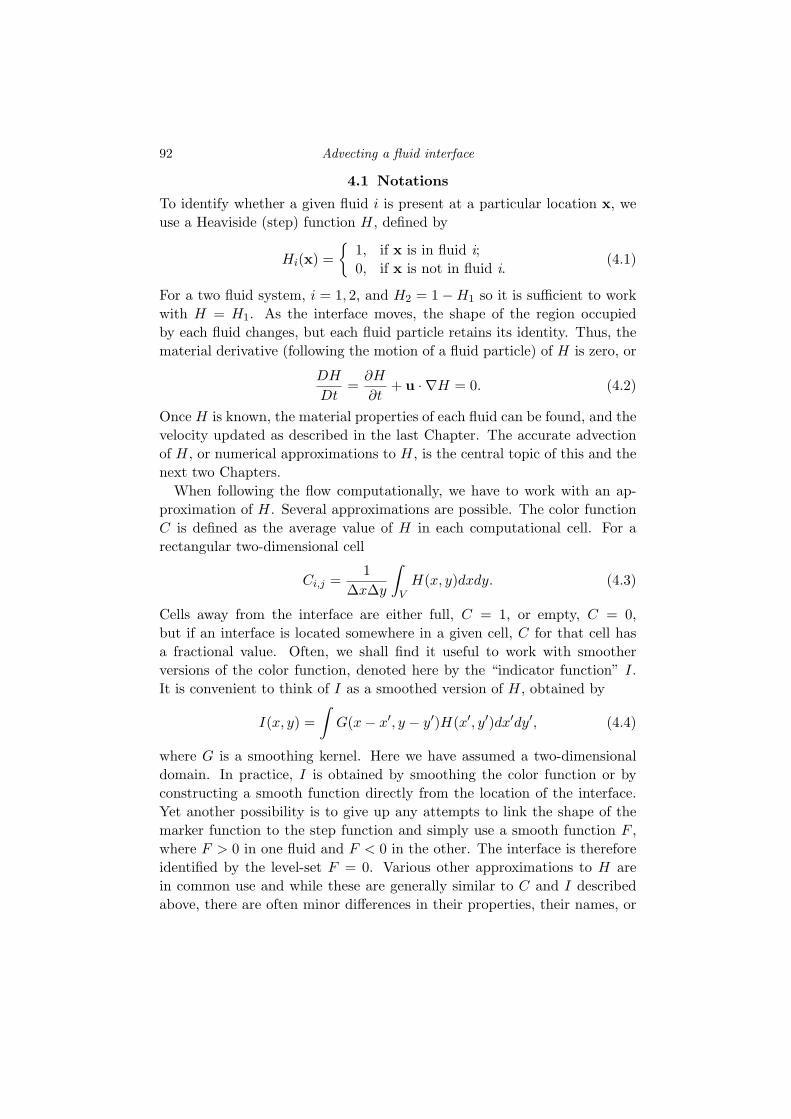
92 Advecting a fluid interface
4.1 NotationsTo identify whether a given fluid i is present at a particular location x, weuse a Heaviside (step) function H, defined by
Hi(x) =�
1, if x is in fluid i;0, if x is not in fluid i.
(4.1)
For a two fluid system, i = 1, 2, and H2 = 1−H1 so it is sufficient to workwith H = H1. As the interface moves, the shape of the region occupiedby each fluid changes, but each fluid particle retains its identity. Thus, thematerial derivative (following the motion of a fluid particle) of H is zero, or
DH
Dt=
∂H
∂t+ u ·∇H = 0. (4.2)
Once H is known, the material properties of each fluid can be found, and thevelocity updated as described in the last Chapter. The accurate advectionof H, or numerical approximations to H, is the central topic of this and thenext two Chapters.
When following the flow computationally, we have to work with an ap-proximation of H. Several approximations are possible. The color functionC is defined as the average value of H in each computational cell. For arectangular two-dimensional cell
Ci,j =1
∆x∆y
�
VH(x, y)dxdy. (4.3)
Cells away from the interface are either full, C = 1, or empty, C = 0,but if an interface is located somewhere in a given cell, C for that cell hasa fractional value. Often, we shall find it useful to work with smootherversions of the color function, denoted here by the “indicator function” I.It is convenient to think of I as a smoothed version of H, obtained by
I(x, y) =�
G(x− x�, y − y�)H(x�, y�)dx�dy�, (4.4)
where G is a smoothing kernel. Here we have assumed a two-dimensionaldomain. In practice, I is obtained by smoothing the color function or byconstructing a smooth function directly from the location of the interface.Yet another possibility is to give up any attempts to link the shape of themarker function to the step function and simply use a smooth function F ,where F > 0 in one fluid and F < 0 in the other. The interface is thereforeidentified by the level-set F = 0. Various other approximations to H arein common use and while these are generally similar to C and I describedabove, there are often minor differences in their properties, their names, or

4.2 Advecting the color function 93
j-1 !j !j+1!
j-1/2 !j+1/2!
F(x)!
I(x)!
Figure 4.1!
H(x)!
Cj!
Fig. 4.1. Different representations of an interface on a grid. The solid line representsa step function H, the shaded function is the color function Cj , and the dashed lineis a smooth indicator function I. The dash-dot line is a level-set function whosezero contour marks the interface.
their physical interpretation. With this in mind, we will use c for the phase-field variable in Section 4.6 and f for the CIP marker function in Section4.7.
Figure 4.1 shows a few different ways to identify the interface. The Heav-iside function H(x) is the discontinuous function shown by a solid line thatchanges abruptly from H = 1 to H = 0 in cell j, exactly where the interfaceis located. The color function Cj , the average value of the marker in eachcell, is shown by the shaded area, and the smooth approximation I(x) isshown by the dashed line. Notice that H and C are identical everywhereexcept in the interface cell j, but that I approaches a uniform value moreslowly. The level-set function F (x), defined such that |F | = d where d isthe distance from the interface, is shown by a dashed-dot line. While H, I,and F obviously vary with x, Cj is inherently identified with cell j. In thediscussion below we will, however, sometimes talk about C as a continuousfunction approximated by the Cjs in each cell.
4.2 Advecting the color function
It is perhaps somewhat counterintuitive that the seemingly simple problemof pushing a piecewise-constant function around by a prescribed velocityfield, using the linear first order advection equation, should be one of thehard problems in computational science. The difficulty is even more surpris-ing given the deceptive simplicity of the one-dimensional problem. Yet, theone-dimensional problem can serve as both an introduction to the difficultiesas well as a motivation for the various techniques that have been designedto overcome the difficulties. We shall therefore examine the one-dimensionalproblem in some detail here. To simplify our task, we assume that the flow

94 Advecting a fluid interface
is incompressible so that the velocity is constant, u = uo > 0. The advectionof the color function is therefore governed by
∂C
∂t+
∂F
∂x= 0, (4.5)
where F = uoC is the flux function. As the interface moves to the right,C flows into cell j through the left boundary and out through the rightboundary. For cell j we denote the left and the right boundaries by j − 1/2and j + 1/2, respectively, and the fluxes by Fj−1/2 and Fj+1/2. If the valueof C in cell j at time level n is denoted by Cn
j and the value at the end of atime step ∆t by Cn+1
j , then we can write:
Cn+1j = Cn
j −1
∆x
� t+∆t
t(Fj+1/2 − Fj−1/2) dt. (4.6)
Or, in words, the change in Cj is the difference between what flows in andwhat flows out of cell j. Here, Fj−1/2 = uoCj−1/2 and Fj+1/2 = uoCj+1/2
and the key challenge is to accurately estimate Cj−1/2 and Cj+1/2.If we take C in each cell to be a constant, then the integration of the
fluxes over time is simple. The value of C that crosses the j−1/2 boundaryis simply the value in the cell to the left, Cj−1, and the value of C crossingthe j + 1/2 boundary is Cj . Thus, as long as we limit the size of each timestep to ∆tuo ≤ ∆x, we can update Cj by
Cn+1j = Cn
j −uo∆t
∆x(Cj − Cj−1). (4.7)
In Fig. 4.2 we show the advection of C using this scheme. The initialcondition is a blob of constant C that should move to the right by a constantvelocity without changing its shape. The exact solution is shown at timet = 0, t = 140∆t, and t = 280∆t, along with the solution advected usingthe scheme above (equation 4.7 using 200 equal-sized control volumes fora domain of length 1, blob width of 20∆x, and ∆t = 0.5∆x). Obviously,scheme (4.7) does a terrible job. Even though the blob has only moved twiceits length it has diffused excessively and as it moves further it continues todiffuse. What went wrong? We used the exact fluxes, so the problem cannotbe there. The culprit is the assumption that the correct way to computethe flux of C is to represent the distribution of C in each cell by the cellaverage Cj . Since C is supposed to approximate H we do not want any Cto flow out of cell j until it is full. Thus, if cell j is initially half full, sothe interface is in middle, and we take a time step ∆t = uo∆x/4 so thatthe interface moves to the left boundary, then cell j should be full and cellj + 1 should still be empty at the end of the step. The problem is therefore
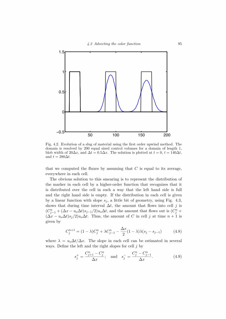
4.2 Advecting the color function 95
50 100 150 2000.5
0
0.5
1
1.5
Fig. 4.2. Evolution of a slug of material using the first order upwind method. Thedomain is resolved by 200 equal sized control volumes for a domain of length 1,blob width of 20∆x, and ∆t = 0.5∆x. The solution is plotted at t = 0, t = 140∆t,and t = 280∆t.
that we computed the fluxes by assuming that C is equal to its average,everywhere in each cell.
The obvious solution to this smearing is to represent the distribution ofthe marker in each cell by a higher-order function that recognizes that itis distributed over the cell in such a way that the left hand side is fulland the right hand side is empty. If the distribution in each cell is givenby a linear function with slope sj , a little bit of geometry, using Fig. 4.3,shows that during time interval ∆t, the amount that flows into cell j is(Cn
j−1 + (∆x− uo∆t)sj−1/2)uo∆t, and the amount that flows out is (Cnj +
(∆x − uo∆t)sj/2)uo∆t. Thus, the amount of C in cell j at time n + 1 isgiven by
Cn+1j = (1− λ)Cn
j + λCnj−1 −
∆x
2(1− λ)λ(sj − sj−1) (4.8)
where λ = uo∆t/∆x. The slope in each cell can be estimated in severalways. Define the left and the right slopes for cell j by
s+j =
Cnj+1 − Cn
j
∆x; and s−j =
Cnj − Cn
j−1
∆x. (4.9)
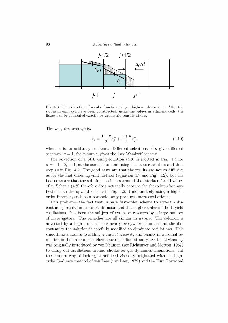
96 Advecting a fluid interface
j-1/2 j+1/2
tu0 tsj-1
sj
j-1 j j+1
Figure 4.3
Fig. 4.3. The advection of a color function using a higher-order scheme. After theslopes in each cell have been constructed, using the values in adjacent cells, thefluxes can be computed exactly by geometric considerations.
The weighted average is:
sj =1− κ
2s−j +
1 + κ
2s+j , (4.10)
where κ is an arbitrary constant. Different selections of κ give differentschemes. κ = 1, for example, gives the Lax-Wendroff scheme.
The advection of a blob using equation (4.8) is plotted in Fig. 4.4 forκ = −1, 0, +1, at the same times and using the same resolution and timestep as in Fig. 4.2. The good news are that the results are not as diffusiveas for the first order upwind method (equation 4.7 and Fig. 4.2), but thebad news are that the solutions oscillates around the interface for all valuesof κ. Scheme (4.8) therefore does not really capture the sharp interface anybetter than the upwind scheme in Fig. 4.2. Unfortunately using a higher-order function, such as a parabola, only produces more oscillations.
This problem—the fact that using a first-order scheme to advect a dis-continuity results in excessive diffusion and that higher-order methods yieldoscillations—has been the subject of extensive research by a large numberof investigators. The remedies are all similar in nature. The solution isadvected by a high-order scheme nearly everywhere, but around the dis-continuity the solution is carefully modified to eliminate oscillations. Thissmoothing amounts to adding artificial viscosity and results in a formal re-duction in the order of the scheme near the discontinuity. Artificial viscositywas originally introduced by von Neuman (see Richtmyer and Morton, 1967)to damp out oscillations around shocks for gas dynamics simulations, butthe modern way of looking at artificial viscosity originated with the high-order Godunov method of van Leer (van Leer, 1979) and the Flux Corrected

4.2 Advecting the color function 97
50 100 150 2000.5
0
0.5
1
1.5
Fig. 4.4. Evolution of a slug of material using higher-order methods. All parametersare the same as in figure 4.2.
Transport method (Boris and Book, 1973). While modern shock capturingmethods have reached a high degree of sophistication and do, in particular,capture shocks in compressible flows very well, they are usually not entirelysatisfactory for the advection of a passive marker function, particularly for along time. Shocks in compressible flows generally “want” to remain sharp†and slight smoothing of the shock is immediately repaired. For a passivemarker there is no inherent mechanism that sharpens a smoothed interfaceand the flow does not “know” the difference between an absolutely sharpinterface and a smoother one. Thus, shocks are generally captured betterthan contact discontinuities in simulations of compressible flows. For theadvection of a marker function, advanced monotonicity-preserving methodsfor shock capturing work well for short times, but for longer times differentapproaches are needed.
† since characteristics flow into the shock

98 Advecting a fluid interface
j-1/2 j+1/2xCj x+u0 t- x
u0 t
j-1 j j+1
Figure 4.5
Fig. 4.5. One-dimensional advection by the Volume of Fluid method. Given thevalue of the color function in the interface cell j, and the side where the full cell is,the location of the interface can be found and the fluxes computed exactly.
4.3 The Volume-of-Fluid (VOF) method
While high-order monotonicity-preserving methods have been a great suc-cess for computations of flows with shocks, their success in solving equation(4.5) is mixed at best—although we should acknowledge that for relativelyshort times, the best of these methods do just fine. For the long time evo-lution of a marker function we have to step back, take a fresh look at theproblem of advecting the color function C, and seek a different way of doingso.
In one-dimension, as depicted in Fig. 4.5, the answer is embarrassinglysimple. Cj is either 0 or 1, except in an interface cell, so the value of Cj
in the interface cell yields immediately the exact location of the interface.If Cj−1 = 1, Cj = 1/3, and Cj+1 = 0 the interface is ∆x/3 from the leftboundary. If Cj = 1/2, the interface is in the middle of the cell, and soforth. If uo ≥ 0 the flux through the left boundary is always uo and we cancompute exactly the flux through the right boundary, since we know theexact location of the interface. If uo∆t < (1 − Cj)∆x, the flux is zero andif uo∆t > (1 − Cj)∆x the flux is first zero and then uo after the interfacereaches the left boundary. Thus,� t+∆t
tFj+1/2 dt =
�0, ∆t ≤ (1− Cj)∆x/uo;(Cj − 1)∆x + uo∆t, ∆t > (1− Cj)∆x/uo.
(4.11)
This expression was used to compute the exact motion of the blob in Figs.4.2 and 4.4.
Thus, for one-dimensional problems the advection of the marker functionis essentially trivial. Not so in higher dimensions! The first attempt to ex-tend the advection described by equation (4.11) to higher dimension was the

4.3 The Volume-of-Fluid (VOF) method 99
Simple Line Interface Calculation, or SLIC, method of Noh and Woodward(1976). In this approach the marker function is advected by time splittingwhere we advect first in one coordinate direction and then in the other (as-suming two-dimensional flow). For advection in the horizontal direction, aninterface cell is divided by a vertical line into a full part and an empty part,with the decision of which side is empty and which is full depending on thevolume fraction in the cells to the left and the right. Once the location of theinterface has been determined, the time integration of the fluxes is done us-ing equation (4.11). The interface is then advected in the vertical directionby dividing the cell by a horizontal line into a full and an empty part. Inthree dimensions this process obviously must also be repeated for the thirdcoordinate direction. Hirt and Nichols (1981) proposed a slightly differentmethod where the interface was still approximated by straight lines, parallelto the coordinate axis, but the same orientation was used for the advectionin the different coordinate directions. To determine whether the interfaceshould be horizontal or vertical, Hirt and Nichols found the normal to theinterface, using values of C in the neighboring cells, and selected the orien-tation of the interface depending on whether the normal was more closelyaligned with the horizontal or the vertical axis. Although perhaps moreappealing than the original SLIC method, tests by Rudman (1997) suggestthat the Hirt and Nichols method is not significantly more accurate. Inaddition to distorting the interfaces, both methods generally generate con-siderable amount of “floatsam” and “jetsam” where pieces of the interfacebreak away in an unphysical way.
Although the method of Hirt and Nichols perhaps did not improve sig-nificantly on the SLIC approach, it nevertheless suggested that the key toimproving the behavior of the advection scheme was the reconstruction ofthe interface in each cell, using the values of the marker function in each cell,along with the value in the neighboring cells. In the Piecewise Linear Inter-face Calculation (PLIC) method introduced by DeBar (1974) and Youngs(1982), the interface is approximated by a straight line segment in each cell,but the line can be oriented arbitrarily with respect to the coordinate axis.The orientation of the line is determined by the normal to the interface,which is found by considering the average value of C in both the cell underconsideration as well as the adjacent cells. Once the interface in each cell hasbeen constructed, the fluxes from one cell to another are computed by geo-metric considerations. The result of the advection generally depends on theaccuracy of the interface reconstruction and finding the normal accuratelytherefore becomes critical for PLIC methods. Several methods have beenproposed to do so. Given C in each cell and the normals, the exact loca-

100 Advecting a fluid interface
a b
c d
Fig. 4.6. VOF reconstruction of the solution for advection in two-dimensions. (a)The original interface. (b) The original SLIC reconstruction. (c) The Hirt andNichols reconstruction. (d) PLIC reconstruction. Figure adapted from Rudman(1997).
tion of the interface can be determined. In two dimensions the line segmentcan cross any of two adjacent or opposite cell faces, so there are four basicinterface configurations. In three dimensions there are many more possibleconfigurations, adding considerably to the complexity of the method.
Figure 4.6, adapted from Rudman (1997), shows the main difference be-tween the interface reconstruction using SLIC, the Hirt and Nichols VOFmethod, and PLIC. While the linear reconstruction captures slowly varyingsections of the interface very well, it usually does less well for interfacesthat are changing rapidly. Notice that the line segments are not continuousacross cell boundaries.
In the next Chapter we discuss modern VOF methods in detail, and laterin the book we will show several examples of computations done using VOFmethods.

4.4 Front Tracking 101
Figure 4.7
Fig. 4.7. When using a Front-Tracking method the fluid interface is representedby connected marker particles that are advected by the fluid velocity, interpolatedfrom the fixed grid.
4.4 Front Tracking
Instead of advecting a marker function by reconstructing the location of theinterface in a partially full cell, for one-dimensional problems we can, ofcourse, simply use a marker point that is moved with the imposed velocity.If the interface is located at xf , then the amount of Cj in the interface cell isgiven exactly by Cj = (xf − xj−1/2)/∆x. We can also construct a smootherapproximations to the step function by setting the cell values as a func-tion of the distance to the interface. In one dimension both approaches areequally straightforward. For two- and three-dimensional problems, we needto use many marker points that are connected to represent a curve (in two-dimensions) or a surface (in three-dimensions). Figure 4.7 shows schemat-ically the representation of an interface using connected marker points, intwo dimensions.
The use of connected marker points in simulations of the motion of a fluidinterface in viscous fluids goes back to Daly (1969b), who used the points tocompute surface tension in MAC simulations of the Rayleigh-Taylor instabil-ity. The use of marker points to track shocks was discussed by Richtmyer andMorton (1967) who appear to have introduced the term “Front Tracking,”but they neither showed nor referenced any implementations. Glimm and
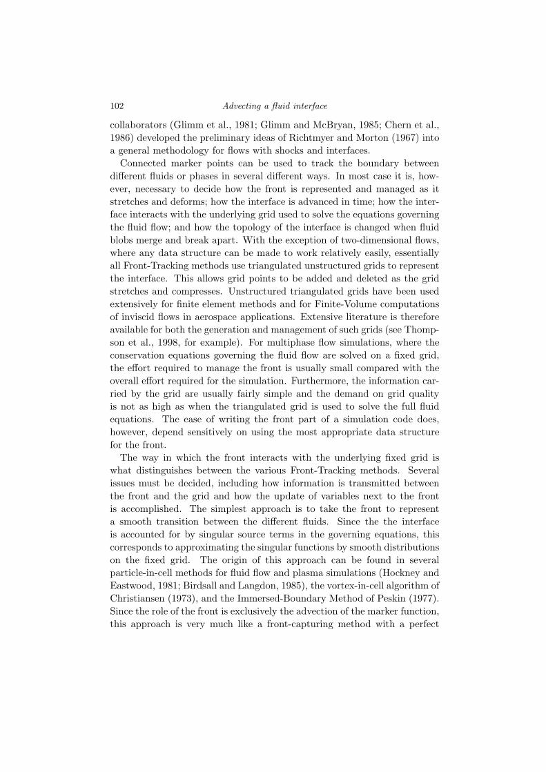
102 Advecting a fluid interface
collaborators (Glimm et al., 1981; Glimm and McBryan, 1985; Chern et al.,1986) developed the preliminary ideas of Richtmyer and Morton (1967) intoa general methodology for flows with shocks and interfaces.
Connected marker points can be used to track the boundary betweendifferent fluids or phases in several different ways. In most case it is, how-ever, necessary to decide how the front is represented and managed as itstretches and deforms; how the interface is advanced in time; how the inter-face interacts with the underlying grid used to solve the equations governingthe fluid flow; and how the topology of the interface is changed when fluidblobs merge and break apart. With the exception of two-dimensional flows,where any data structure can be made to work relatively easily, essentiallyall Front-Tracking methods use triangulated unstructured grids to representthe interface. This allows grid points to be added and deleted as the gridstretches and compresses. Unstructured triangulated grids have been usedextensively for finite element methods and for Finite-Volume computationsof inviscid flows in aerospace applications. Extensive literature is thereforeavailable for both the generation and management of such grids (see Thomp-son et al., 1998, for example). For multiphase flow simulations, where theconservation equations governing the fluid flow are solved on a fixed grid,the effort required to manage the front is usually small compared with theoverall effort required for the simulation. Furthermore, the information car-ried by the grid are usually fairly simple and the demand on grid qualityis not as high as when the triangulated grid is used to solve the full fluidequations. The ease of writing the front part of a simulation code does,however, depend sensitively on using the most appropriate data structurefor the front.
The way in which the front interacts with the underlying fixed grid iswhat distinguishes between the various Front-Tracking methods. Severalissues must be decided, including how information is transmitted betweenthe front and the grid and how the update of variables next to the frontis accomplished. The simplest approach is to take the front to representa smooth transition between the different fluids. Since the the interfaceis accounted for by singular source terms in the governing equations, thiscorresponds to approximating the singular functions by smooth distributionson the fixed grid. The origin of this approach can be found in severalparticle-in-cell methods for fluid flow and plasma simulations (Hockney andEastwood, 1981; Birdsall and Langdon, 1985), the vortex-in-cell algorithm ofChristiansen (1973), and the Immersed-Boundary Method of Peskin (1977).Since the role of the front is exclusively the advection of the marker function,this approach is very much like a front-capturing method with a perfect

4.4 Front Tracking 103
(or nearly perfect) advection scheme. While information must be passedbetween the front and the grid, the smoothing of the interface alleviates theneed for any modification of the solution method for the fluid equations nearthe interface (except that the solver must be written for material propertiesthat vary spatially). For finite-Reynolds-number multiphase flows, Unverdiand Tryggvason (1992) developed a method where the front is used both toupdate the marker function and to include surface tension. Their methodhas been used to study a wide variety of multiphase flows and we describeit in more detail in Chapter 6.
To avoid smoothing the interface, but still use a fixed grid for the solutionof the conservation equations, it is necessary to modify the numerical ap-proximations near the front. In Glimm’s Front-Tracking method, the fieldvariables at the front are extrapolated to grid points on the other side ofthe front, allowing the use of regular finite-difference discretizations for gridpoints next to an interface. A similar approach is used in the Ghost-Fluidmethod of Fedkiw et al. (1999), although the interface tracking is done usinga Level-Set method instead of connected marker particles. As discussed byGlimm et al. (2001), the extrapolation can be done in several different ways,but in all cases the contribution from the ghost points results in the equiv-alence of source terms in the discrete governing equations. This is also thecase in the Immersed-Interface Method of Lee and LeVeque (2003) wherethe jump conditions at the front are incorporated directly into the numericalapproximations for gradients evaluated near the front, on the fixed grid.
Another approach to keep the interface sharp is the modification of thefixed grid near the front in such a way that the grid lines coincide withthe interface. This generally leads to irregularly-shaped control volumesnear the interface and often involves merging some of the control volumesto eliminate very small ones. The origin of this approach is the “cut cell”methods initially developed for aerospace applications (see Powell, 1998, forexample), but its application to multiphase flow simulations was originatedby Udaykumar et al. (1997). See also Udaykumar et al. (1999), Udaykumaret al. (2001), Liu et al. (2005) and Marella et al. (2005). Since the jumpconditions can be imposed directly at the cell boundary, this method is,in many ways, similar to using two separate grids for each phase. We do,however, mention it here as most of the grid is left unchanged.
One of the main objections to the use of Front-Tracking methods is thattopology changes, where fluid regions merge or breakup, are not handled au-tomatically, as in methods where the marker function is advected directly.Changing the connection of the front points can obviously be accomplished,but at the cost of increased code complexity. When two interfaces come close

104 Advecting a fluid interface
together, the film between them can sometimes become very thin and rup-ture. However, it may or may not be appropriate to fuse interfaces togetherwhen the film is of the order of one grid spacing. In Front Tracking the in-terfaces never fuse together unless something special is done and sometimesthe added level of control provided by the tracking is desirable. The questionof how interfaces merge is still not a completely resolved issue as discussedin Chapter 2, and we will return to how to handle it computationally at theend of Chapter 6.
4.5 The Level-Set methodIn the Level-Set method the different fluid regions are identified by a smoothmarker function, F (x, t) which is positive in one fluid and negative in theother. The boundary between the fluids is identified by the F (x, t) = 0 levelcurve. The level-set function moves with the fluid and therefore evolvesaccording to
∂F
∂t+ u ·∇F = 0. (4.12)
The motion of the zero level-set curve depends only on the normal velocitycomponent. The normal can be found by
n = −∇F
|∇F |. (4.13)
Substituting for ∇F in equation (4.12) and using that u · n = Vn results in
∂F
∂t− Vn|∇F | = 0 (4.14)
which is an alternate expression for the advection of F .Unlike the C function in the VOF method, the level-set marker function
is smooth and it can therefore—at least in principle—be advected using anystandard method for hyperbolic equations. Most authors have, however,used high order schemes such as the ENO method of Osher and Shu (1991).
To reconstruct the material properties of the flow (density and viscosity,for example), a marker function is constructed from F
I(F ) =
0, if F < −α∆x;12(1 + (F/α∆x) + 1
π sin(πF/α∆x)), if |F | ≤ α∆x;1, if F > α∆x.
(4.15)
Here ∆x is the size of a grid cell and α is an empirical coefficient, oftentaken to be equal to 3, giving an interface thickness of about 6 cells. Thus,I changes from 0 to 1 over only a few cells, describing a smooth transition

4.5 The Level-Set method 105
zone from one fluid to the next. Once I has been constructed, the variousmaterial properties can be assigned. Given I(x), we can generate a smoothedgrid delta function at the interface by taking its gradient
δ = ∇I =dI
dF∇F. (4.16)
The mapping in equation (4.15) requires the use of the values of F off theF = 0 contour (or level set). For the thickness of the transition zone toremain approximately constant, F must have the same shape near the in-terface for all times. If F is simply advected by the fluid, this is not usuallythe case. Where the interface is stretched the gradient of F becomes steeperand where the interface is compressed the gradient becomes smaller. Todeal with this problem, Sussman et al. (1994) introduced a reinitializationprocedure where they modified F by solving
∂F
∂τ+ sgn(Fo)(|∇F |− 1) = 0 (4.17)
at each time step. Here, sgn is the sign function and F0 is the un-reinitializedlevel-set function. τ is a pseudo-time and equation (4.17) is integrated tosteady state, thus enforcing |∇F | = 1. This makes F a distance functionand ensures that the slope near the interface is always the same. For slowly-moving interfaces the level-set function only needs to be re-initialized everyonce in a while, but for more rapidly moving interfaces it may have to bereinitialized at every time step. The re-initialization can result in an artifi-cial motion of the interface which can contribute to poor mass conservation.Several improvements have therefore been proposed, including approximat-ing the sgn function using a smoother function. Peng et al. (1999) proposedreplacing sgn(Fo) in equation (4.17) by
S(F ) =F�
F 2 + |∇F |2∆x2(4.18)
and applying (4.17) at every time step. As long as the level-set functiontakes a large positive or negative values far away from the interface, thereconstruction only needs to be done near the F = 0 contour. Since thesolution to equation (4.17) propagates outward from the interface, whereF is given, the solution is first corrected there and it is usually sufficienttake only a few steps in pseudo time. The reconstruction of the level-setfunction as a distance function was critical in making level sets work forfluid dynamics simulations. As Osher and Fedkiw (2001) point out, re-initialization is still an active area of research.
For fluid-dynamics problems the F function is generally advected by the

106 Advecting a fluid interface
fluid velocity. In other applications, such as the motion of a solidificationfront, the velocity is only defined at the interface and must be extended offthe interface to advect the level-set function. The extension of the velocitiesoff the interface has been the subject of several papers, including Chen et al.(1997b) who showed that the velocity field known at the interface could beextended into the region around the interface by using an upwind methodto solve
∂S
∂τ+ S(F )n ·∇S = 0 (4.19)
for each velocity component (taking S = u, v, or w). This process results ina velocity field that is constant in a direction normal to the interface. As forthe reinitalization of the level-set function as a distance function (equation4.17), the velocity field only needs to be constructed in the neighborhood ofthe F = 0 contour.
The Level-Set method, at least in its original embodiment, has the ap-peal of simplicity. For a fluid mechanics problem one only has to solve oneadditional partial differential equation and there are essentially no addi-tional complex steps, such as the reconstruction of an interface in the VOFmethod, or the addition of new computational objects such as when FrontTracking is used. This simplicity has, however, come at some cost and earlyimplementations had considerable problems with mass conservation. Whilemany of the early difficulties have been overcome, efforts to generate moreaccurate methods generally result in added complexity. This has eroded themain appeal of Level-Set methods and made them more comparable to otherapproaches, both in terms of complexity and performance.
For further discussions of the Level-Set method, the reader is referred toSussman et al. (1998) who proposed a way to improve the mass conserva-tion; Sussman and Puckett (2000), who introduced a hybrid VOF/Level-Set method, sometimes known by its acronym CLSVOF; and Fedkiw et al.(1999) who developed a “ghost fluid” method based on assigning fictiousvalues to grid points on the other side of a fluid discontinuity. For generalreviews of the Level-Set method, see Osher and Fedkiw (2002) and Sethian(2001).
4.6 Phase-Field methodsIn the Phase-Field method, the interface is kept relatively sharp by a modi-fication of the governing equations. The interface is assumed to be of a finitethickness and described by thermodynamically consistent conservation laws.In actual implementations, however, the thickness of the transition is much

4.6 Phase-Field methods 107
larger than it is in real systems and it is not clear whether keeping thethermodynamic conditions correct in an artificially thick interface has anyadvantages over methods that model the behavior in the transition zone inother ways. The Phase-Field approach has found widespread use in sim-ulation of solidification, but its use for fluid dynamic simulations is morelimited.
To update the phase function c, which identifies the different fluids, anonlinear diffusion term is added to the advection equation, resulting in theso-called Cahn-Hilliard equation with advection. The diffusion terms smearsout an interface that is becoming thinner due to straining but an antidiffusivepart prevents the interface from becoming too thick, such as if the interfaceis compressed. The Navier-Stokes equations are also modified by adding aterm that results in surface tension in the interface zone. The key to themodification is the introduction of a free-energy function and by selectingthe function in the proper way—including the appropriate values for thevarious adjustable coefficients—it is possible to ensure that the thickness ofthe interface remains of the same order as the grid spacing.
For a two-fluid system where the two fluids have similar densities (sothe Boussinesq approximation can be used) and same viscosity and massdiffusion coefficient, Jacqmin (1999) solved
ρ0DuDt
= −∇S + µ∇2u− c∇φ + gρ(c) (4.20)
for the fluid velocity and updated the phase-field variable by
Dc
Dt= κ∇2φ. (4.21)
Here, κ is a diffusion coefficient and the potential φ is derived from the freeenergy of the fluid by
φ = βdψ(c)
dc− α∇2c, (4.22)
where ψ(c) = (c + 1/2)2(c − 1/2)2. The coefficients α and β describe therelative importance of the “gradient” energy and bulk energy density. Itcan be shown that the thickness of the phase boundary is O(α/β) and sur-face tension is proportional to
√αβ. S is a pressure-like variable used to
enforce incompressibility. For any given grid spacing ∆x, we must selectthe appropriate diffusion coefficient κ as well as α and β. For the ψ usedabove, Jacqmin (1999) showed that the surface tension is σ =
�αβ/18 and
that the interface thickness �, defined as the 90% variation of c, is given by� ≈ 4.164
�α/β. Thus, if surface tension and interface thickness are given
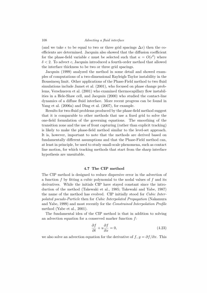
108 Advecting a fluid interface
(and we take � to be equal to two or three grid spacings ∆x) then the co-efficients are determined. Jacqmin also showed that the diffusion coefficientfor the phase-field variable c must be selected such that κ = O(�δ) whereδ < 2. To advect c, Jacqmin introduced a fourth-order method that allowedthe interface thickness to be two or three grid spacings.
Jacqmin (1999) analyzed the method in some detail and showed exam-ples of computations of a two-dimensional Rayleigh-Taylor instability in theBoussinesq limit. Other applications of the Phase-Field method to two fluidsimulations include Jamet et al. (2001), who focused on phase change prob-lems, Verschueren et al. (2001) who examined thermocapillary flow instabil-ities in a Hele-Shaw cell, and Jacqmin (2000) who studied the contact-linedynamics of a diffuse fluid interface. More recent progress can be found inYang et al. (2006a) and Ding et al. (2007), for example.
Results for two-fluid problems produced by the phase-field method suggestthat it is comparable to other methods that use a fixed grid to solve theone-field formulation of the governing equations. The smoothing of thetransition zone and the use of front capturing (rather than explicit tracking)is likely to make the phase-field method similar to the level-set approach.It is, however, important to note that the methods are derived based onfundamentally different assumptions and that the Phase-Field method can,at least in principle, be used to study small-scale phenomena, such as contactline motion, for which tracking methods that start from the sharp interfacehypothesis are unsuitable.
4.7 The CIP method
The CIP method is designed to reduce dispersive error in the advection ofa function f by fitting a cubic polynomial to the nodal values of f and itsderivatives. While the initials CIP have stayed constant since the intro-duction of the method (Takewaki et al., 1985; Takewaki and Yabe, 1987)the name of the method has evolved. CIP initially stood for Cubic Inter-polated pseudo-Particle then for Cubic Interpolated Propagation (Nakamuraand Yabe, 1999) and most recently for the Constrained Interpolation Profilemethod (Yabe et al., 2001).
The fundamental idea of the CIP method is that in addition to solvingan advection equation for a conserved marker function f :
∂f
∂t+ u
∂f
∂x= 0, (4.23)
we also solve an advection equation for the derivative of f , g = ∂f/∂x. This
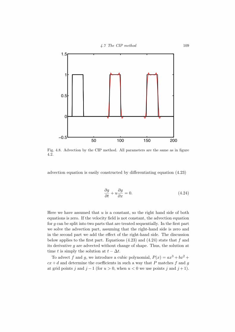
4.7 The CIP method 109
50 100 150 2000.5
0
0.5
1
1.5
Fig. 4.8. Advection by the CIP method. All parameters are the same as in figure4.2.
advection equation is easily constructed by differentiating equation (4.23)
∂g
∂t+ u
∂g
∂x= 0. (4.24)
Here we have assumed that u is a constant, so the right hand side of bothequations is zero. If the velocity field is not constant, the advection equationfor g can be split into two parts that are treated sequentially. In the first partwe solve the advection part, assuming that the right-hand side is zero andin the second part we add the effect of the right-hand side. The discussionbelow applies to the first part. Equations (4.23) and (4.24) state that f andits derivative g are advected without change of shape. Thus, the solution attime t is simply the solution at t−∆t.
To advect f and g, we introduce a cubic polynomial, P (x) = ax3 + bx2 +cx + d and determine the coefficients in such a way that P matches f and gat grid points j and j− 1 (for u > 0, when u < 0 we use points j and j +1).
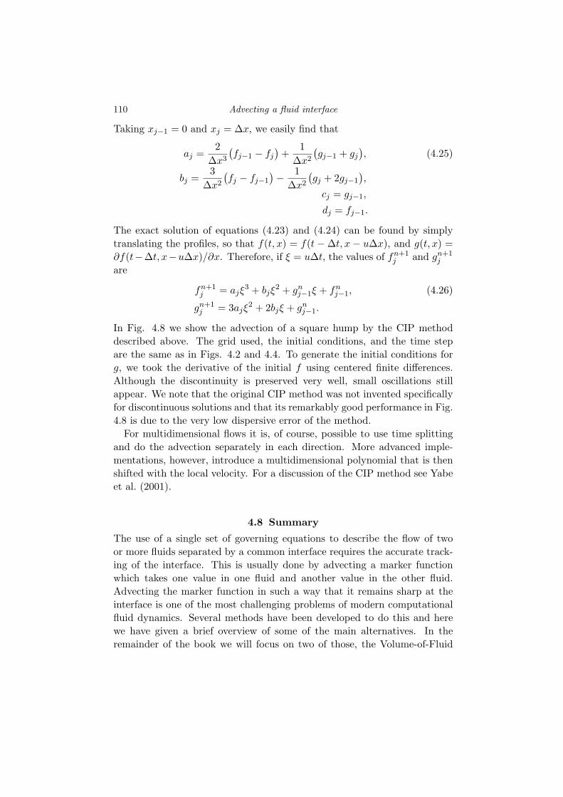
110 Advecting a fluid interface
Taking xj−1 = 0 and xj = ∆x, we easily find that
aj =2
∆x3
�fj−1 − fj
�+
1∆x2
�gj−1 + gj
�, (4.25)
bj =3
∆x2
�fj − fj−1
�−
1∆x2
�gj + 2gj−1
�,
cj = gj−1,
dj = fj−1.
The exact solution of equations (4.23) and (4.24) can be found by simplytranslating the profiles, so that f(t, x) = f(t−∆t, x− u∆x), and g(t, x) =∂f(t−∆t, x−u∆x)/∂x. Therefore, if ξ = u∆t, the values of fn+1
j and gn+1j
are
fn+1j = ajξ
3 + bjξ2 + gn
j−1ξ + fnj−1, (4.26)
gn+1j = 3ajξ
2 + 2bjξ + gnj−1.
In Fig. 4.8 we show the advection of a square hump by the CIP methoddescribed above. The grid used, the initial conditions, and the time stepare the same as in Figs. 4.2 and 4.4. To generate the initial conditions forg, we took the derivative of the initial f using centered finite differences.Although the discontinuity is preserved very well, small oscillations stillappear. We note that the original CIP method was not invented specificallyfor discontinuous solutions and that its remarkably good performance in Fig.4.8 is due to the very low dispersive error of the method.
For multidimensional flows it is, of course, possible to use time splittingand do the advection separately in each direction. More advanced imple-mentations, however, introduce a multidimensional polynomial that is thenshifted with the local velocity. For a discussion of the CIP method see Yabeet al. (2001).
4.8 SummaryThe use of a single set of governing equations to describe the flow of twoor more fluids separated by a common interface requires the accurate track-ing of the interface. This is usually done by advecting a marker functionwhich takes one value in one fluid and another value in the other fluid.Advecting the marker function in such a way that it remains sharp at theinterface is one of the most challenging problems of modern computationalfluid dynamics. Several methods have been developed to do this and herewe have given a brief overview of some of the main alternatives. In theremainder of the book we will focus on two of those, the Volume-of-Fluid

4.8 Summary 111
(VOF) method and the Front-Tracking method of Unverdi and Tryggvason(1992). The VOF method is the most widely used method to directly ad-vect the marker function. While early implementations may not have beenable to capture interfaces accurately, major improvements have been madeand these methods are now capable of producing solutions comparable tothe best of the more recent alternatives. Although some of the alternative,such as level sets, have gained popularity because of their apparent simplic-ity, effort to increase their accuracy generally result in added complexity,thus reducing their appeal when compared to the VOF method. The mostadvanced methods to directly advect a marker function on a fixed grid arecurrently capable of producing solutions of a quality comparable to earlyimplementations of front-tracking methods. However, the accuracy of front-tracking methods can also be improved and it is probably fair to say thatfor comparable computational effort, the use of interface markers will alwaysyield superior results. Such methods are, however, more complex and it islikely that methods where the marker function is advected on a fixed gridwill remain more popular for the foreseeable future.