Multinomial + Cont. JointChris Piech

CS109, Stanford University

CS109 Flow

Discrete Joint Distributions:General Case

Multinomial: A parametric Discrete Joint

Cont. Joint Distributions: General Case

Today

1. Know how to use a multinomial2. Be able to calculate large bayes problems using a computer

3. Use a Joint CDF

Learning Goals

Motivating Examples

Four Prototypical Trajectories

Recall logs

Log Review

log(x) = y implies ey = xlog(x) = y implies ey = x

Log Identities

log(a · b) = log(a) + log(b)

log(a/b) = log(a)� log(b)

log(an) = n · log(a)

Products become Sums!

log(Y

i

ai) =X

i

log(ai)

log(a · b) = log(a) + log(b)

* Spoiler alert: This is important because the product of many small numbers gets hard for computers to represent.

Four Prototypical Trajectories

Where we left off

Joint Probability Table

Roommates 2RoomDblShared Partner Single

Frosh 0.30 0.07 0.00 0.00 0.37Soph 0.12 0.18 0.00 0.03 0.32Junior 0.04 0.01 0.00 0.10 0.15Senior 0.01 0.02 0.02 0.01 0.05

5+ 0.02 0.00 0.05 0.04 0.110.49 0.27 0.07 0.18 1.00

Prob

abili

ty

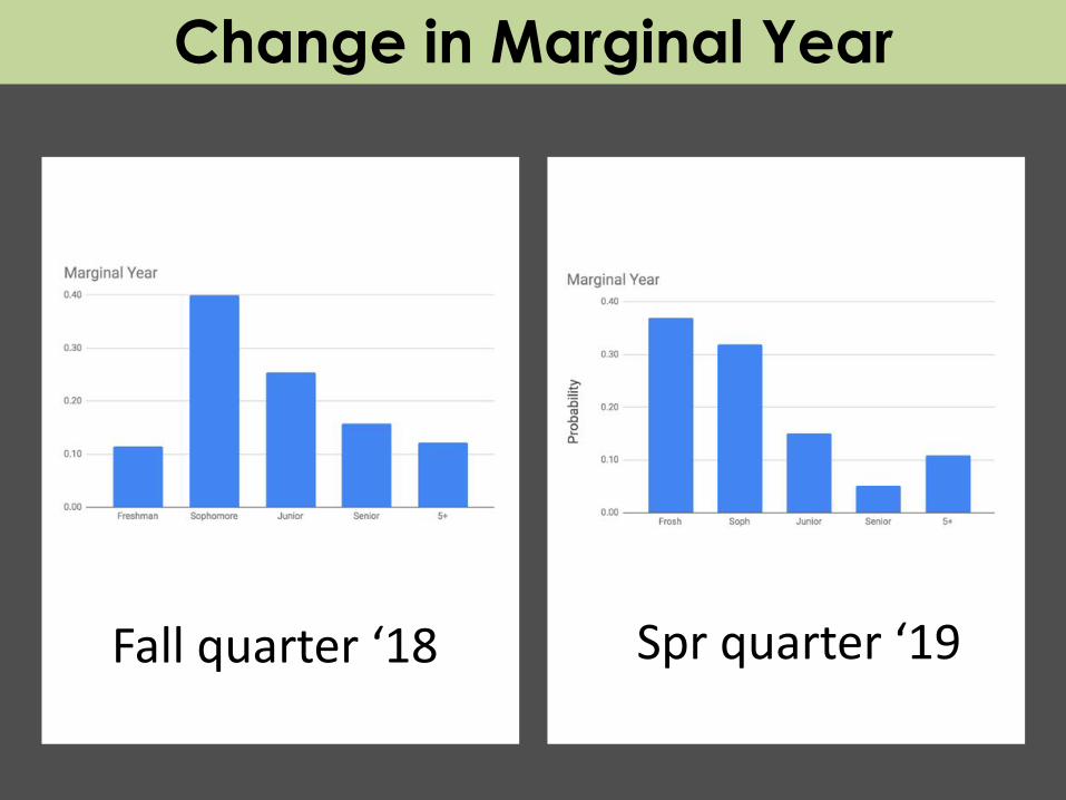
Change in Marginal Year

Fall quarter ‘18 Spr quarter ‘19

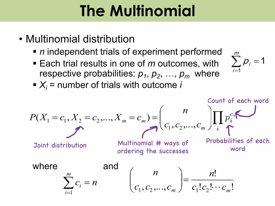
• Multinomial distribution§ n independent trials of experiment performed§ Each trial results in one of m outcomes, with

respective probabilities: p1, p2, …, pm where§ Xi = number of trials with outcome i

where and

mcm

cc

mmm ppp

cccn

cXcXcXP ...,...,,

),...,,( 2121

212211 ÷÷

ø

öççè

æ====

ncm

ii =å

=1!!!

!,...,, 2121 mm ccc

nccc

n×××

=÷÷ø

öççè

æ

The Multinomial

Joint distribution Multinomial # ways of ordering the successes

Probabilities of each ordering are equal and

mutually exclusive

å=

=m

iip

11

• Multinomial distribution§ n independent trials of experiment performed§ Each trial results in one of m outcomes, with

respective probabilities: p1, p2, …, pm where§ Xi = number of trials with outcome i

where and

å=

=m

iip

11

ncm

ii =å

=1!!!

!,...,, 2121 mm ccc

nccc

n×××

=÷÷ø

öççè

æ

The Multinomial

Joint distribution Multinomial # ways of ordering the successes

Probabilities of each word

P (X1 = c1, . . . Xm = cm) =

✓n

c1, . . . , cm

◆Y

i

pcii<latexit sha1_base64="CoIhbDQWH6rpHTi6qJXKQj2YbFg=">AAACNnicbVDLSgMxFM3UV62vUZdugkWoUMqMCHYjFNy4ESrYB7R1yKRpG5rHkGSEMsxXufE73HXjQhG3foLptAttvRByOOfcm9wTRoxq43lTJ7e2vrG5ld8u7Ozu7R+4h0dNLWOFSQNLJlU7RJowKkjDUMNIO1IE8ZCRVji+memtJ6I0leLBTCLS42go6IBiZCwVuHf1Ujvw4TXEgV+G3b40GrYDnhH83F6JgF08klITmMw8maVsxTSF3UjJfkBhFNBHK9I0cItexcsKrgJ/AYpgUfXAfbXzcMyJMJghrTu+F5legpShmJG00I01iRAeoyHpWCgQJ7qXZGun8MwyfTiQyh5hYMb+7kgQ13rCQ+vkyIz0sjYj/9M6sRlUewkVUWyIwPOHBjGDRsJZhrBPFcGGTSxAWFH7V4hHSCFsbNIFG4K/vPIqaF5UfK/i318Wa9VFHHlwAk5BCfjgCtTALaiDBsDgGUzBO/hwXpw359P5mltzzqLnGPwp5/sHF8WpSA==</latexit><latexit sha1_base64="CoIhbDQWH6rpHTi6qJXKQj2YbFg=">AAACNnicbVDLSgMxFM3UV62vUZdugkWoUMqMCHYjFNy4ESrYB7R1yKRpG5rHkGSEMsxXufE73HXjQhG3foLptAttvRByOOfcm9wTRoxq43lTJ7e2vrG5ld8u7Ozu7R+4h0dNLWOFSQNLJlU7RJowKkjDUMNIO1IE8ZCRVji+memtJ6I0leLBTCLS42go6IBiZCwVuHf1Ujvw4TXEgV+G3b40GrYDnhH83F6JgF08klITmMw8maVsxTSF3UjJfkBhFNBHK9I0cItexcsKrgJ/AYpgUfXAfbXzcMyJMJghrTu+F5legpShmJG00I01iRAeoyHpWCgQJ7qXZGun8MwyfTiQyh5hYMb+7kgQ13rCQ+vkyIz0sjYj/9M6sRlUewkVUWyIwPOHBjGDRsJZhrBPFcGGTSxAWFH7V4hHSCFsbNIFG4K/vPIqaF5UfK/i318Wa9VFHHlwAk5BCfjgCtTALaiDBsDgGUzBO/hwXpw359P5mltzzqLnGPwp5/sHF8WpSA==</latexit><latexit sha1_base64="CoIhbDQWH6rpHTi6qJXKQj2YbFg=">AAACNnicbVDLSgMxFM3UV62vUZdugkWoUMqMCHYjFNy4ESrYB7R1yKRpG5rHkGSEMsxXufE73HXjQhG3foLptAttvRByOOfcm9wTRoxq43lTJ7e2vrG5ld8u7Ozu7R+4h0dNLWOFSQNLJlU7RJowKkjDUMNIO1IE8ZCRVji+memtJ6I0leLBTCLS42go6IBiZCwVuHf1Ujvw4TXEgV+G3b40GrYDnhH83F6JgF08klITmMw8maVsxTSF3UjJfkBhFNBHK9I0cItexcsKrgJ/AYpgUfXAfbXzcMyJMJghrTu+F5legpShmJG00I01iRAeoyHpWCgQJ7qXZGun8MwyfTiQyh5hYMb+7kgQ13rCQ+vkyIz0sjYj/9M6sRlUewkVUWyIwPOHBjGDRsJZhrBPFcGGTSxAWFH7V4hHSCFsbNIFG4K/vPIqaF5UfK/i318Wa9VFHHlwAk5BCfjgCtTALaiDBsDgGUzBO/hwXpw359P5mltzzqLnGPwp5/sHF8WpSA==</latexit><latexit sha1_base64="CoIhbDQWH6rpHTi6qJXKQj2YbFg=">AAACNnicbVDLSgMxFM3UV62vUZdugkWoUMqMCHYjFNy4ESrYB7R1yKRpG5rHkGSEMsxXufE73HXjQhG3foLptAttvRByOOfcm9wTRoxq43lTJ7e2vrG5ld8u7Ozu7R+4h0dNLWOFSQNLJlU7RJowKkjDUMNIO1IE8ZCRVji+memtJ6I0leLBTCLS42go6IBiZCwVuHf1Ujvw4TXEgV+G3b40GrYDnhH83F6JgF08klITmMw8maVsxTSF3UjJfkBhFNBHK9I0cItexcsKrgJ/AYpgUfXAfbXzcMyJMJghrTu+F5legpShmJG00I01iRAeoyHpWCgQJ7qXZGun8MwyfTiQyh5hYMb+7kgQ13rCQ+vkyIz0sjYj/9M6sRlUewkVUWyIwPOHBjGDRsJZhrBPFcGGTSxAWFH7V4hHSCFsbNIFG4K/vPIqaF5UfK/i318Wa9VFHHlwAk5BCfjgCtTALaiDBsDgGUzBO/hwXpw359P5mltzzqLnGPwp5/sHF8WpSA==</latexit>

Count of each wordmcm

cc

mmm ppp

cccn

cXcXcXP ...,...,,

),...,,( 2121

212211 ÷÷

ø

öççè

æ====

• 6-sided die is rolled 7 times§ Roll results: 1 one, 1 two, 0 three, 2 four, 0 five, 3 six

• This is generalization of Binomial distribution§ Binomial: each trial had 2 possible outcomes§ Multinomial: each trial has m possible outcomes

7302011654321

61420

61

61

61

61

61

61

!3!0!2!0!1!1!7

)3,0,2,0,1,1(

÷øö

çèæ=÷

øö

çèæ

÷øö

çèæ

÷øö

çèæ

÷øö

çèæ

÷øö

çèæ

÷øö

çèæ=

====== XXXXXXP

Hello Die Rolls, My Old Friends

According to the Global Language Monitor there are 988,968 words in the english language used on the internet.

The

Probabilistic Text Analysis

Example document:“Pay for Viagra with a credit-card. Viagra is great. So are credit-cards. Risk free Viagra. Click for free.”n = 18

Text is a Multinomial

Viagra = 2Free = 2Risk = 1Credit-card: 2…For = 2

P

✓1

2|spam

◆=

n!

2!2! . . . 2!p2viagrap

2free . . . p

2forP

✓1

2|spam

◆=

n!

2!2! . . . 2!p2viagrap

2free . . . p

2forP

✓1

2|spam

◆=

n!

2!2! . . . 2!p2viagrap

2free . . . p

2for

Probability of seeing this document | spam

It’s a Multinomial!

The probability of a word in spam email being viagra

Four Prototypical Trajectories

Who wrote the federalist papers?

• Authorship of “Federalist Papers”

§ 85 essays advocating ratification of US constitution

§ Written under pseudonym “Publius”o Really, Alexander Hamilton, James

Madison and John Jay

§ Who wrote which essays?o Analyzed probability of words in each

essay versus word distributions from known writings of three authors

Old and New Analysis

Four Prototypical Trajectories

Let’s write a program!

Example document:“Pay for Viagra with a credit-card. Viagra is great. So are credit-cards. Risk free Viagra. Click for free.”n = 18

Text is a Multinomial

Viagra = 2Free = 2Risk = 1Credit-card: 2…For = 2

P

✓1

2|spam

◆=

n!

2!2! . . . 2!p2viagrap

2free . . . p

2forP

✓1

2|spam

◆=

n!

2!2! . . . 2!p2viagrap

2free . . . p

2forP

✓1

2|spam

◆=

n!

2!2! . . . 2!p2viagrap

2free . . . p

2for

Probability of seeing this document | spam

It’s a Multinomial!

The probability of a word in spam email being viagra

Four Prototypical Trajectories

woot

Continuous Random Variables

Joint Distributions

Four Prototypical Trajectories

Continuous Joint Distribution

Riding the Marguerite

You are running to the bus stop. You don’t know exactly when the bus arrives. You arrive at 2:20pm.

What is P(wait < 5 min)?

Joint Dart Distribution

P(hit within R pixels of center)?

What is the probability that a dart hits at (456.234231234122355, 532.12344123456)?

Joint Dart Distribution

Dart x location

Dar

t y lo

catio

n

0.005

0.12

P(hit within R pixels of center)?

Joint Dart Distribution

Dart x location

Dar

t y lo

catio

n

0.005

0.12

P(hit within R pixels of center)?

Joint Dart Distribution

Dart x location

Dar

t y lo

catio

nP(hit within R pixels of center)?

0

y

x900

900

Joint Dart Distribution

In the limit, as you break down continuous values into intestinally small buckets, you end up with

multidimensional probability density

A joint probability density function gives the relative likelihood of more than one continuous random variable each taking on a specific value.

Joint Probability Density Funciton

0

y

x 900

900

0 900

900

a1a2

b2b1

fX,Y (x, y)

xy

Joint Probability Density Funciton

!

plot by Academo

Joint Probability Density Function

l Let X and Y be two continuous random variables§ where 0 ≤ X ≤ 1 and 0 ≤ Y ≤ 2

l We want to integrate g(x,y) = xy w.r.t. X and Y:§ First, do “innermost” integral (treat y as a constant):

§ Then, evaluate remaining (single) integral:

òòò òò ò=== == =

=úû

ùêë

é=÷÷

ø

öççè

æ=

2

0

2

0

22

0

1

0

2

0

1

0 21

2

0

1

yyy xy x

dyydyx

ydydxxydydxxy

101 42

10

222

0

=-=úû

ùêë

é=ò

=

ydyyy

Multiple Integrals Without Tears

Marginal probabilities give the distribution of a subset of the variables (often, just one) of a joint distribution.

Sum/integrate over the variables you don’t care about.

Marginalization

pX(a) =X

y

pX,Y (a, y)

fX(a) =

1Z

�1

fX,Y (a, y) dy

fY (b) =

1Z

�1

fX,Y (x, b) dx

Marginal probabilities give the distribution of a subset of the variables (often, just one) of a joint distribution.

Sum/integrate over the variables you don’t care about.

Marginalization

pX(a) =X

y

pX,Y (a, y)

fX(a) =

1Z

�1

fX,Y (a, y) dy

fY (b) =

1Z

�1

fX,Y (x, b) dx

Marginal probabilities give the distribution of a subset of the variables (often, just one) of a joint distribution.

Sum/integrate over the variables you don’t care about.

Marginalization

pX(a) =X

y

pX,Y (a, y)

fX(a) =

1Z

�1

fX,Y (a, y) dy

fY (b) =

1Z

�1

fX,Y (x, b) dx

Marginal probabilities give the distribution of a subset of the variables (often, just one) of a joint distribution.

Sum/integrate over the variables you don’t care about.

Marginalization

pX(a) =X

y

pX,Y (a, y)

fX(a) =

1Z

�1

fX,Y (a, y) dy

fY (b) =

1Z

�1

fX,Y (x, b) dx

Darts!

Dart PDF

X-Pixel Marginal

y

xY-Pixel Marginal

X ⇠ N✓900

2,900

2

◆Y ⇠ N

✓900

3,900

5

◆

Cumulative Density Function (CDF):

ò ò¥- ¥-

=a b

YXYX dxdyyxfbaF ),( ),( ,,

),(),( ,

2

, baFbaf YXYX ba ¶¶¶=

Joint Cumulative Density Function

FX,Y (a, b) = P (X < a, Y < b)<latexit sha1_base64="dSeAv8GAi6lbSe+0enumc8Mzb0k=">AAACB3icbVDLSsNAFJ3UV62vqEtBBovQQimJCHahUBDEZQXbprQhTKaTduhkEmYmQgndufFX3LhQxK2/4M6/cdpmoa0HLvdwzr3M3OPHjEplWd9GbmV1bX0jv1nY2t7Z3TP3D1oySgQmTRyxSDg+koRRTpqKKkacWBAU+oy0/dH11G8/ECFpxO/VOCZuiAacBhQjpSXPPL7xUqfSmZRQxS/DK9goOfASogrs6OaXPbNoVa0Z4DKxM1IEGRqe+dXrRzgJCVeYISm7thUrN0VCUczIpNBLJIkRHqEB6WrKUUikm87umMBTrfRhEAldXMGZ+nsjRaGU49DXkyFSQ7noTcX/vG6igpqbUh4ninA8fyhIGFQRnIYC+1QQrNhYE4QF1X+FeIgEwkpHV9Ah2IsnL5PWWdW2qvbdebFey+LIgyNwAkrABhegDm5BAzQBBo/gGbyCN+PJeDHejY/5aM7Idg7BHxifP8fjlV0=</latexit><latexit sha1_base64="dSeAv8GAi6lbSe+0enumc8Mzb0k=">AAACB3icbVDLSsNAFJ3UV62vqEtBBovQQimJCHahUBDEZQXbprQhTKaTduhkEmYmQgndufFX3LhQxK2/4M6/cdpmoa0HLvdwzr3M3OPHjEplWd9GbmV1bX0jv1nY2t7Z3TP3D1oySgQmTRyxSDg+koRRTpqKKkacWBAU+oy0/dH11G8/ECFpxO/VOCZuiAacBhQjpSXPPL7xUqfSmZRQxS/DK9goOfASogrs6OaXPbNoVa0Z4DKxM1IEGRqe+dXrRzgJCVeYISm7thUrN0VCUczIpNBLJIkRHqEB6WrKUUikm87umMBTrfRhEAldXMGZ+nsjRaGU49DXkyFSQ7noTcX/vG6igpqbUh4ninA8fyhIGFQRnIYC+1QQrNhYE4QF1X+FeIgEwkpHV9Ah2IsnL5PWWdW2qvbdebFey+LIgyNwAkrABhegDm5BAzQBBo/gGbyCN+PJeDHejY/5aM7Idg7BHxifP8fjlV0=</latexit><latexit sha1_base64="dSeAv8GAi6lbSe+0enumc8Mzb0k=">AAACB3icbVDLSsNAFJ3UV62vqEtBBovQQimJCHahUBDEZQXbprQhTKaTduhkEmYmQgndufFX3LhQxK2/4M6/cdpmoa0HLvdwzr3M3OPHjEplWd9GbmV1bX0jv1nY2t7Z3TP3D1oySgQmTRyxSDg+koRRTpqKKkacWBAU+oy0/dH11G8/ECFpxO/VOCZuiAacBhQjpSXPPL7xUqfSmZRQxS/DK9goOfASogrs6OaXPbNoVa0Z4DKxM1IEGRqe+dXrRzgJCVeYISm7thUrN0VCUczIpNBLJIkRHqEB6WrKUUikm87umMBTrfRhEAldXMGZ+nsjRaGU49DXkyFSQ7noTcX/vG6igpqbUh4ninA8fyhIGFQRnIYC+1QQrNhYE4QF1X+FeIgEwkpHV9Ah2IsnL5PWWdW2qvbdebFey+LIgyNwAkrABhegDm5BAzQBBo/gGbyCN+PJeDHejY/5aM7Idg7BHxifP8fjlV0=</latexit><latexit sha1_base64="dSeAv8GAi6lbSe+0enumc8Mzb0k=">AAACB3icbVDLSsNAFJ3UV62vqEtBBovQQimJCHahUBDEZQXbprQhTKaTduhkEmYmQgndufFX3LhQxK2/4M6/cdpmoa0HLvdwzr3M3OPHjEplWd9GbmV1bX0jv1nY2t7Z3TP3D1oySgQmTRyxSDg+koRRTpqKKkacWBAU+oy0/dH11G8/ECFpxO/VOCZuiAacBhQjpSXPPL7xUqfSmZRQxS/DK9goOfASogrs6OaXPbNoVa0Z4DKxM1IEGRqe+dXrRzgJCVeYISm7thUrN0VCUczIpNBLJIkRHqEB6WrKUUikm87umMBTrfRhEAldXMGZ+nsjRaGU49DXkyFSQ7noTcX/vG6igpqbUh4ninA8fyhIGFQRnIYC+1QQrNhYE4QF1X+FeIgEwkpHV9Ah2IsnL5PWWdW2qvbdebFey+LIgyNwAkrABhegDm5BAzQBBo/gGbyCN+PJeDHejY/5aM7Idg7BHxifP8fjlV0=</latexit>

!

"

to 0 asx → -∞,y → -∞,

to 1 asx → +∞,y → +∞,

plot by Academo

Joint CDF

FX,Y (a, b) = P (X < a, Y < b)<latexit sha1_base64="dSeAv8GAi6lbSe+0enumc8Mzb0k=">AAACB3icbVDLSsNAFJ3UV62vqEtBBovQQimJCHahUBDEZQXbprQhTKaTduhkEmYmQgndufFX3LhQxK2/4M6/cdpmoa0HLvdwzr3M3OPHjEplWd9GbmV1bX0jv1nY2t7Z3TP3D1oySgQmTRyxSDg+koRRTpqKKkacWBAU+oy0/dH11G8/ECFpxO/VOCZuiAacBhQjpSXPPL7xUqfSmZRQxS/DK9goOfASogrs6OaXPbNoVa0Z4DKxM1IEGRqe+dXrRzgJCVeYISm7thUrN0VCUczIpNBLJIkRHqEB6WrKUUikm87umMBTrfRhEAldXMGZ+nsjRaGU49DXkyFSQ7noTcX/vG6igpqbUh4ninA8fyhIGFQRnIYC+1QQrNhYE4QF1X+FeIgEwkpHV9Ah2IsnL5PWWdW2qvbdebFey+LIgyNwAkrABhegDm5BAzQBBo/gGbyCN+PJeDHejY/5aM7Idg7BHxifP8fjlV0=</latexit><latexit sha1_base64="dSeAv8GAi6lbSe+0enumc8Mzb0k=">AAACB3icbVDLSsNAFJ3UV62vqEtBBovQQimJCHahUBDEZQXbprQhTKaTduhkEmYmQgndufFX3LhQxK2/4M6/cdpmoa0HLvdwzr3M3OPHjEplWd9GbmV1bX0jv1nY2t7Z3TP3D1oySgQmTRyxSDg+koRRTpqKKkacWBAU+oy0/dH11G8/ECFpxO/VOCZuiAacBhQjpSXPPL7xUqfSmZRQxS/DK9goOfASogrs6OaXPbNoVa0Z4DKxM1IEGRqe+dXrRzgJCVeYISm7thUrN0VCUczIpNBLJIkRHqEB6WrKUUikm87umMBTrfRhEAldXMGZ+nsjRaGU49DXkyFSQ7noTcX/vG6igpqbUh4ninA8fyhIGFQRnIYC+1QQrNhYE4QF1X+FeIgEwkpHV9Ah2IsnL5PWWdW2qvbdebFey+LIgyNwAkrABhegDm5BAzQBBo/gGbyCN+PJeDHejY/5aM7Idg7BHxifP8fjlV0=</latexit><latexit sha1_base64="dSeAv8GAi6lbSe+0enumc8Mzb0k=">AAACB3icbVDLSsNAFJ3UV62vqEtBBovQQimJCHahUBDEZQXbprQhTKaTduhkEmYmQgndufFX3LhQxK2/4M6/cdpmoa0HLvdwzr3M3OPHjEplWd9GbmV1bX0jv1nY2t7Z3TP3D1oySgQmTRyxSDg+koRRTpqKKkacWBAU+oy0/dH11G8/ECFpxO/VOCZuiAacBhQjpSXPPL7xUqfSmZRQxS/DK9goOfASogrs6OaXPbNoVa0Z4DKxM1IEGRqe+dXrRzgJCVeYISm7thUrN0VCUczIpNBLJIkRHqEB6WrKUUikm87umMBTrfRhEAldXMGZ+nsjRaGU49DXkyFSQ7noTcX/vG6igpqbUh4ninA8fyhIGFQRnIYC+1QQrNhYE4QF1X+FeIgEwkpHV9Ah2IsnL5PWWdW2qvbdebFey+LIgyNwAkrABhegDm5BAzQBBo/gGbyCN+PJeDHejY/5aM7Idg7BHxifP8fjlV0=</latexit><latexit sha1_base64="dSeAv8GAi6lbSe+0enumc8Mzb0k=">AAACB3icbVDLSsNAFJ3UV62vqEtBBovQQimJCHahUBDEZQXbprQhTKaTduhkEmYmQgndufFX3LhQxK2/4M6/cdpmoa0HLvdwzr3M3OPHjEplWd9GbmV1bX0jv1nY2t7Z3TP3D1oySgQmTRyxSDg+koRRTpqKKkacWBAU+oy0/dH11G8/ECFpxO/VOCZuiAacBhQjpSXPPL7xUqfSmZRQxS/DK9goOfASogrs6OaXPbNoVa0Z4DKxM1IEGRqe+dXrRzgJCVeYISm7thUrN0VCUczIpNBLJIkRHqEB6WrKUUikm87umMBTrfRhEAldXMGZ+nsjRaGU49DXkyFSQ7noTcX/vG6igpqbUh4ninA8fyhIGFQRnIYC+1QQrNhYE4QF1X+FeIgEwkpHV9Ah2IsnL5PWWdW2qvbdebFey+LIgyNwAkrABhegDm5BAzQBBo/gGbyCN+PJeDHejY/5aM7Idg7BHxifP8fjlV0=</latexit>

Jointly Continuous

ò ò=£<£<2

1

2

1

),( ) ,(P ,2121

a

a

b

bYX dxdyyxfbYbaXa

a1a2

b2b1

fX,Y (x, y)

xy

a1

a2

b1

b2

Probabilities from Joint CDF

! "# < % ≤ "',)# < * ≤ )' = ,-,. "',)'

a1

a2

b1

b2

Probabilities from Joint CDF

! "# < % ≤ "',)# < * ≤ )' = ,-,. "',)'

a1

a2

b1

b2

Probabilities from Joint CDF

! "# < % ≤ "',)# < * ≤ )' = ,-,. "',)'

a1

a2

b1

b2

Probabilities from Joint CDF

! "# < % ≤ "',)# < * ≤ )' = ,-,. "',)'−,-,. "#,)'

a1

a2

b1

b2

Probabilities from Joint CDF

! "# < % ≤ "',)# < * ≤ )' = ,-,. "',)'−,-,. "#,)'

a1

a2

b1

b2

Probabilities from Joint CDF

! "# < % ≤ "',)# < * ≤ )' = ,-,. "',)'−,-,. "#,)'−,-,. "',)#

a1

a2

b1

b2

Probabilities from Joint CDF

! "# < % ≤ "',)# < * ≤ )' = ,-,. "',)'−,-,. "#,)'−,-,. "',)#

a1

a2

b1

b2

Probabilities from Joint CDF

! "# < % ≤ "',)# < * ≤ )' = ,-,. "',)'−,-,. "#,)'−,-,. "',)#+,-,. "#,)#

! "# < % ≤ "',)# < * ≤ )' = ,-,. "',)'−,-,. "#,)'−,-,. "',)#+,-,. "#,)#

a1

a2

b1

b2

Probabilities from Joint CDF

Probability for Instagram!

Gaussian BlurIn image processing, a Gaussian blur is the result of blurring an image by a Gaussian function. It is a widely used effect in graphics software, typically to reduce image noise.

Gaussian blurring with StDev = 3, is based on a joint probability distribution:

fX,Y (x, y) =1

2⇡ · 32 e� x2+y2

2·32

FX,Y (x, y) = �⇣x3

⌘· �

⇣y3

⌘

Joint PDF

Joint CDF

Used to generate this weight matrix

Gaussian Blur

fX,Y (x, y) =1

2⇡ · 32 e� x2+y2

2·32

FX,Y (x, y) = �⇣x3

⌘· �

⇣y3

⌘

Joint PDF

Joint CDF

Each pixel is given a weight equal to the probability that X and Y are both within the pixel bounds. The center pixel covers the area where

-0.5 ≤ x ≤ 0.5 and -0.5 ≤ y ≤ 0.5What is the weight of the center pixel?

P (�0.5 < X < 0.5,�0.5 < Y < 0.5)

=P (X < 0.5, Y < 0.5)� P (X < 0.5, Y < �0.5)

� P (X < �0.5, Y < 0.5) + P (X < �0.5, Y < �0.5)

=�

✓0.5

3

◆· �

✓0.5

3

◆� 2�

✓0.5

3

◆· �

✓�0.5

3

◆

+ �

✓�0.5

3

◆· �

✓�0.5

3

◆

=0.56622 � 2 · 0.5662 · 0.4338 + 0.43382 = 0.206

P (�0.5 < X < 0.5,�0.5 < Y < 0.5)

=P (X < 0.5, Y < 0.5)� P (X < 0.5, Y < �0.5)

� P (X < �0.5, Y < 0.5) + P (X < �0.5, Y < �0.5)

=�

✓0.5

3

◆· �

✓0.5

3

◆� 2�

✓0.5

3

◆· �

✓�0.5

3

◆

+ �

✓�0.5

3

◆· �

✓�0.5

3

◆

=0.56622 � 2 · 0.5662 · 0.4338 + 0.43382 = 0.206

P (�0.5 < X < 0.5,�0.5 < Y < 0.5)

=P (X < 0.5, Y < 0.5)� P (X < 0.5, Y < �0.5)

� P (X < �0.5, Y < 0.5) + P (X < �0.5, Y < �0.5)

=�

✓0.5

3

◆· �

✓0.5

3

◆� 2�

✓0.5

3

◆· �

✓�0.5

3

◆

+ �

✓�0.5

3

◆· �

✓�0.5

3

◆

=0.56622 � 2 · 0.5662 · 0.4338 + 0.43382 = 0.206

P (�0.5 < X < 0.5,�0.5 < Y < 0.5)

=P (X < 0.5, Y < 0.5)� P (X < 0.5, Y < �0.5)

� P (X < �0.5, Y < 0.5) + P (X < �0.5, Y < �0.5)

=�

✓0.5

3

◆· �

✓0.5

3

◆� 2�

✓0.5

3

◆· �

✓�0.5

3

◆

+ �

✓�0.5

3

◆· �

✓�0.5

3

◆

=0.56622 � 2 · 0.5662 · 0.4338 + 0.43382 = 0.206

P (�0.5 < X < 0.5,�0.5 < Y < 0.5)

=P (X < 0.5, Y < 0.5)� P (X < 0.5, Y < �0.5)

� P (X < �0.5, Y < 0.5) + P (X < �0.5, Y < �0.5)

=�

✓0.5

3

◆· �

✓0.5

3

◆� 2�

✓0.5

3

◆· �

✓�0.5

3

◆

+ �

✓�0.5

3

◆· �

✓�0.5

3

◆

=0.56622 � 2 · 0.5662 · 0.4338 + 0.43382 = 0.206

P (�0.5 < X < 0.5,�0.5 < Y < 0.5)

=P (X < 0.5, Y < 0.5)� P (X < 0.5, Y < �0.5)

� P (X < �0.5, Y < 0.5) + P (X < �0.5, Y < �0.5)

=�

✓0.5

3

◆· �

✓0.5

3

◆� 2�

✓0.5

3

◆· �

✓�0.5

3

◆

+ �

✓�0.5

3

◆· �

✓�0.5

3

◆

=0.56622 � 2 · 0.5662 · 0.4338 + 0.43382 = 0.206

Weight Matrix

0

y

x900

900

How do you integrate under a circle?

Four Prototypical Trajectories

Have a great weekend!