Munich Personal RePEc Archive

Multidimensional structural

transformation index: a new measure of

development

Kelbore, Zerihun Getachew

University of South Africa

22 December 2014

Online at https://mpra.ub.uni-muenchen.de/62920/

MPRA Paper No. 62920, posted 18 Mar 2015 09:59 UTC

Multidimensional Structural Transformation Index: A New Measure of

Development

Zerihun Getachew Kelbore

University of South Africa, Bureau of Market Research

Pretoria, South Africa

Email: zehagu@gmail.com

Abstract

Achieving structural transformation is believed to be a priority agenda in development policy of developing

countries. However, the discussion of structural transformation has been bound to an analysis of labor shifts

and productivity convergence between economic sectors. This narrow definition of structural transformation

neglects the vital aspect of structural transformation: social transformation. This study tries to fill this gap by

proposing a multidimensional structural transformation index (STI). The proposed index measures structural

transformation in two phases based on economic and socio-demographic indicators. This multidimensional

indicator may contribute to the development literature as it can be used to measure the extent of structural

transformation across economies and overtime.

The investigation of the relationships of the STIs with the GDP per capita revealed that the STI based on

economic and social dimensions appears to have greater effect on GDP per capita than STI focusing on

economic indicators. The implication of this is that structural transformation containing social transformation

as its priority is essential to achieve inclusive growth, sustain structural transformation, significantly reduce

poverty, and hence enhance economic development.

Each of the STI is a single number lying between 0 and 1, where 0 indicates lack of structural transformation

and 1 complete transformation. The index is mathematically consistent, easy to compute, and comparable

across countries overtime.

Key words: Structural Transformation Index, Normalized Euclidean Distance, Inverse Euclidean Distance,

Factor/Principal Components Analysis

2

1. Introduction

Structural change has been considered as one of the essential ingredients of modern economic growth. As a

stylized fact in development economics literature, structural change is defined as a reallocation of economic

activity across three broad sectors of the economy (agriculture, industry, and services) that accompany the

process of modern economic growth. The reallocation, induced by some policy measures, occurs as factors of

production moved from lower productivity to higher productivity uses (Lewis, 1954; Chenery H. , 1986). For

Kuznets structural changes not only in economic but also in social institutions and beliefs are required for

modern economic growth (Kuznets, 1971). In line with Kuznets, Chenery indicated that economic

development is a result of a set of interrelated changes in the structure of an economy that is required for its

continued growth (Chenery, 1979).

It is believed that in poor countries, where there is disequilibrium in factor returns across sectors, the

reallocation of resources to sectors of higher productivity contributes to growth. This belief among

development economists resulted in a proposition that structural change and economic growth are strongly

interrelated. The possible implications of this hypothesis in development policy attracted the attention of

early development economists including Fisher, Clark, Lewis, Kuznets, and Chenery, among others.

Despite the indications by (Kuznets, 1971), of the essence of social transformation in addition to economic

transformation, studies so far concentrated on and made structural transformation synonymous to economic

transformation. The possible reason for the relegation of the social aspect of the transformation in the

analysis of structural transformation may relate to a dearth of data or lack of interest on social

transformation indicators as an essential part of the required transformation. However, as we discuss in the

theoretical framework (Section 2 of this paper), modern economic growth is much more than mere economic

transformation, and a disruptive process. Various sectors of the economy grow at different rates and hence

the groups of the population attached to the slow growing sectors lose out relatively to those in faster

growing sectors(Syrquin, 1988). To this effect, policy actions and institutional changes are essential

ingredients of the transformation in order to minimize the costs of, and resistance to, the disruptive process

of the high rates of economic growth and structural transformation. Thus, the role of the state (sovereign

state) in managing the transformation is that it has to act as a clearing house for necessary institutional

innovations; as an agency for resolution of conflicts among group of interests; and as a major entrepreneur

for the socially required infrastructure ( (Kuznets, 1971).1

Structural transformation is on the spotlight in Africa`s development policy agenda. As it is one of the

manifestations of the modern economic growth as well as a mechanism to sustain the economic growth,

understanding the structure of the African economies and designing policies that pave the way to growth

promoting structural transformation is what Africa needs today.

To this end, the proposed new multidimensional measure of structural transformation in Africa, called

structural transformation index (STI), measures the extent of structural transformation in African economies

and indicates the aspects of structural transformation that hinder the pace of the transformation. The STI

helps in guiding policy design, infrastructure investment decision, and political commitment to speed up the

transition out of poverty and to an inclusive growth in which the benefits are equally shared among citizens

in each of the countries. It may also help in indicating areas where donors and development partners can

substantially influence and contribute towards achieving the goals of structural transformation and poverty

reduction. .

The United Nations Economic Commission for Africa`s Economic Report on Africa (2014) discusses structural

transformation in Africa measured by changes in the shares of rural labor force in total labor and the share of

agriculture in GDP during 1960—2008 and found that the transformation has lagged far behind that of other

developing regions, especially East Asia and Latin America. With quite a small share of GDP from agriculture

and the rural labor force accounting around 20% of the total labor, the Latin American countries appear to

1 Syrquin (1988) calls this intervention “minimal development state”, although its role goes beyond the one in classical liberal theory where the role of the state is limited to the functions of protecting all its citizens against

violence, theft, and fraud and to the enforcement of contracts, and so on.

3

reflect the most advanced stages of structural transformation compared with the other developing regions

such as East Asia and Pacific, South Asia, and Africa(excluding North Africa). Whereas structural

transformation in Africa remains limited, and the data show that still share of rural population is high, and the

downward trend as a function of income per worker is limited and inconsistent. Agriculture`s share of GDP in

Africa has declined as a function of income per capita, with a nearly linear trend (UNECA, 2014).

The path Africa is going through differs from other developing regions. In the case of East Asia and Latin

America as the structural transformation occurs we observe a trend towards convergence of the rural

population share with the agricultural value added share of GDP as income grows. This distinction is

important due to its implication on rural-urban income disparities. The rural-urban income disparity,

consequently, dies out as the structural transformation leads the rural population share to converge

downwards to the agricultural value added share of GDP. This is the path that Africa is yet to follow (UNECA,

2014).

The remaining parts of the paper are organized as follows, Section 2 discusses the theoretical framework of

the proposed index; Section 3 elaborates the methodological framework and data; Section 4 provides results

and discussion; and Section 5 concludes.

2. Theoretical Framework

Modern analysis of sectoral transformation originated with Fisher (1935, 1939) and Clark (1940), and dealt

with sectoral shifts in the composition of the labor force(Syrquin, 1988).2 However, in the later years, studies

of long run transformation by Kuznets established the stylized facts of structural transformation. The stylized

facts that focus on economic aspect of the transformation are organized into two measures of structural

transformation namely, production and consumption measures. Although both measures are equally

important, in this paper the focus is on the production measure per se due to lack of comparable cross

country data on consumption expenditure for African countries.3

The production measure of structural transformation analyzes the sectoral changes in the employment and

value added shares in the gross domestic product (GDP) as economies grow. That is, structural

transformation is said to occur when the increase in GDP per capita is associated with a decrease in both the

employment share and the nominal value added share in agriculture, and increases in both employment

share and the nominal value added share in services and industry.

However, following (Kuznets, 1971) and (Timmer & Akkus, 2008) this paper adopts a wider framework in the

analysis of structural transformation and constructs a composite indicator of structural transformation

encompassing economic, social, and political dimensions of the transformation.

The guiding framework of the proposed measure of structural transformation takes into account the broader

definition of structural transformation and constitutes the following dimensions as its building blocks. First, it

starts with the production measures of structural transformation and analyses the shifts in sectoral

composition as an indication of structural transformation. In this regard, we take sectoral shares of value

added in GDP and consider each of the sectoral shares as indicators of structural transformation and compare

the observed shifts in sectoral compositions against the stylized facts. The other important aspect of

structural transformation under the production measure approach is the changes in employment shares

among the sectors. This measure, though empirically appealing, is not included in the construction of the STI

due to irregularities of data overtime and across countries.

2 They are the first to deal with the process of reallocation during the epoch of modern economic growth, and to use the form of

sectoral division of (primary—secondary—tertiary), which later on Kuznets categorized as agriculture, industry, and service. 3 In the case of consumption measures final consumption expenditure shares are used as a measure of economic activity at the

sectoral level. Although both the consumption and production measures are used interchangeably in the literature, in fact, there is

a distinction between the two measures. The difference mainly comes from the fundamental distinction between production and

final consumption; and the consumption measure includes investment, import, and export.

4

Second, as a departure from the conventional measures of structural transformation, we incorporate the

socio-demographic indicators as a measure of structural transformation. The socio-demographic dimensions

are captured by the level of urbanization, demographic transition, and human capital accumulation. The

rationale behind these measures is that as the historical evidence shows high rates of growth in per capita

income in the developed world were accompanied by rapid shifts in production and social structure mainly

referred to as industrialization and/or urbanization accompanied by shifts in demographic patterns, an

increasing input into human capital through formal education, and shifts in sets of values that largely conform

to the opportunities and requirements associated with modern urban life.

We consider urbanization as an outcome of structural transformation and take it as one of the multiple

dimensions that enable us track the level of structural transformation of economies. The demographic

transition from high fertility/high mortality rate to low fertility/low mortality is also considered as one

aspect of structural transformation.

3. Methodology for constructing Structural Transformation Index Composite indicators which compare country performance are increasingly recognized as a useful tool in

policy analysis and public communication. They provide simple comparisons of countries that can be used to

illustrate complex and sometimes elusive issues in wide ranging fields such as environment, economy, society

or technological development.

It often seems easier for the general public to interpret composite indicators than to identify common trends

across many separate indicators, and they have also proven useful in benchmarking country performance

(Saltelli, 2007). This is because composite indicator provides a clue to the matter of larger significance or

makes it perceptible a trend or phenomenon that is not immediately (Hammond, Adriaanse, Rodenburg,

Bryant, & Woodward, 1995).

As structural transformation is multidimensional, it needs to be evaluated along several dimensions and has

to be presented in a way which is comprehensive, easy to understand and interpret. To this end, we follow a

multidimensional approach to construct a structural transformation index. Our approach is similar to the

approaches adopted by the UNDP for the construction of Human Development Index (HDI) and Financial

Inclusion Index (Sarma, 2012). As indicated by OECD (2008), we have built a theoretical framework that

guides the construction of the structural transformation index (STI) and in the following we provide a

methodology to compute the indicators of each dimension that constitute the composite indicator.

Each of the indicators is selected based on the theoretical framework and normalized to make them

comparable. The indicators are normalized using a Mini-Max Normalization method and compare the

performance within the continent, Africa.

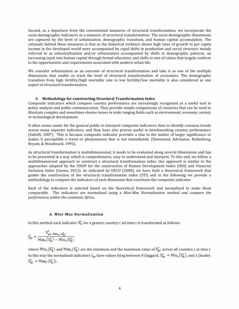
A. Mini-Max Normalization

In this method each indicator for a generic country c nd time t is transformed as follows:

where and are the minimum and the maximum value of across all counties c at time t.

In this way the normalized indicators have values lying between 0 (laggard, , and 1 (leader,

.

5

Thus the higher the value of the higher the country`s achievement in indicator i. If n dimensions of

structural transformation are considered, then, a country`s achievements in these dimensions will be

represented by a point S= (I1, I2,…., In) on the n-dimensional space. On the n-dimensional space, the point O= (0, 0,…, 0) represents the point indicating the worst situation while the point P=(1, 1,…., 1) represents an idea situation indicating the highest achievement in all indicators.

B. Weighting

We applied a factor analysis to generate the weights. Factor analysis groups together individual indicators,

which are collinear to form a composite indicator, that captures as much as possible of the information

common to individual indicators. Each factor, estimated using the principal components analysis, reveals the

set of indicators with which it has the strongest association. In doing so, the factor analysis helps in

accounting for the highest variation in the indicator set using the smallest possible number of factors. As a

result, the composite indicator no longer depends upon the dimensionality of the data set but rather is based on the “statistical” dimensions of the data(OECD, 2008). However, the weight generated using factor analysis

is not a measure of the theoretical importance of the indictors associated with the composite indicator; it only

corrects the overlapping information between two or more correlated indictors.

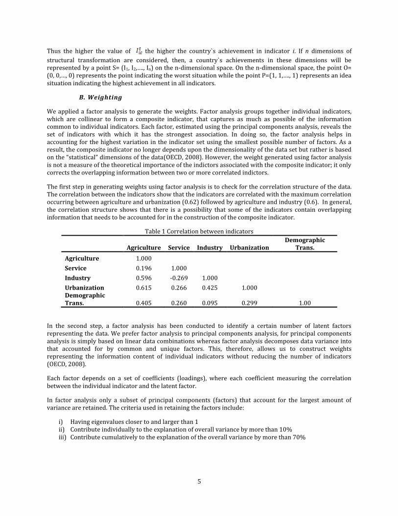
The first step in generating weights using factor analysis is to check for the correlation structure of the data.

The correlation between the indicators show that the indicators are correlated with the maximum correlation

occurring between agriculture and urbanization (0.62) followed by agriculture and industry (0.6). In general,

the correlation structure shows that there is a possibility that some of the indicators contain overlapping

information that needs to be accounted for in the construction of the composite indicator.

Table 1 Correlation between indicators

Agriculture Service Industry Urbanization

Demographic

Trans.

Agriculture 1.000

Service 0.196 1.000

Industry 0.596 -0.269 1.000

Urbanization 0.615 0.266 0.425 1.000

Demographic

Trans. 0.405 0.260 0.095 0.299 1.00

In the second step, a factor analysis has been conducted to identify a certain number of latent factors

representing the data. We prefer factor analysis to principal components analysis, for principal components

analysis is simply based on linear data combinations whereas factor analysis decomposes data variance into

that accounted for by common and unique factors. This, therefore, allows us to construct weights

representing the information content of individual indicators without reducing the number of indicators

(OECD, 2008).

Each factor depends on a set of coefficients (loadings), where each coefficient measuring the correlation

between the individual indicator and the latent factor.

In factor analysis only a subset of principal components (factors) that account for the largest amount of

variance are retained. The criteria used in retaining the factors include:

i) Having eigenvalues closer to and larger than 1

ii) Contribute individually to the explanation of overall variance by more than 10%

iii) Contribute cumulatively to the explanation of the overall variance by more than 70%

6

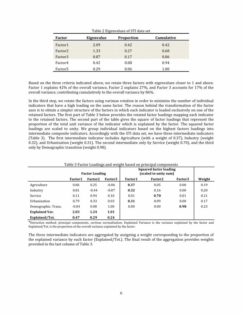
Table 2 Eigenvalues of STI data set

Factor Eigenvalue Proportion Cumulative

Factor1 2.09 0.42 0.42

Factor2 1.33 0.27 0.68

Factor3 0.87 0.17 0.86

Factor4 0.42 0.08 0.94

Factor5 0.29 0.06 1.00

Based on the three criteria indicated above, we retain three factors with eigenvalues closer to 1 and above.

Factor 1 explains 42% of the overall variance, Factor 2 explains 27%, and Factor 3 accounts for 17% of the

overall variance, contributing cumulatively to the overall variance by 86%.

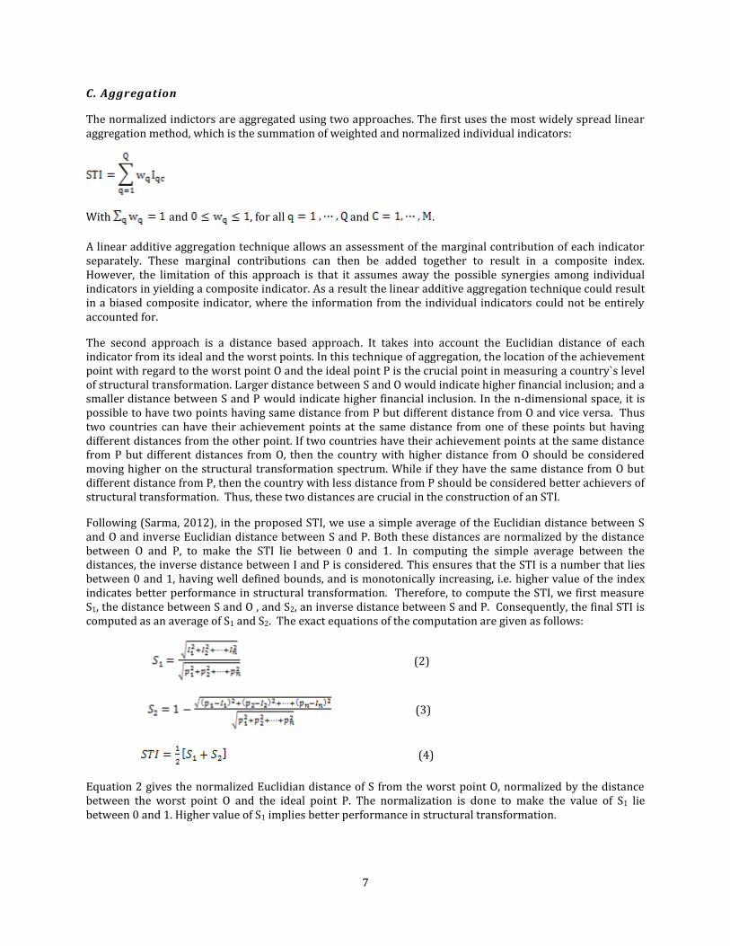
In the third step, we rotate the factors using varimax rotation in order to minimize the number of individual

indicators that have a high loading on the same factor. The reason behind the transformation of the factor

axes is to obtain a simpler structure of the factors in which each indicator is loaded exclusively on one of the

retained factors. The first part of Table 3 below provides the rotated factor loadings mapping each indicator

to the retained factors. The second part of the table gives the square of factor loadings that represent the

proportion of the total unit variance of the indicator which is explained by the factor. The squared factor

loadings are scaled to unity. We group individual indicators based on the highest factors loadings into

intermediate composite indicators. Accordingly with the STI data set, we have three intermediate indicators

(Table 3). The first intermediate indicator includes Agriculture (with a weight of 0.37), Industry (weight

0.32), and Urbanization (weight 0.31). The second intermediate only by Service (weight 0.70), and the third

only by Demographic transition (weight 0.98).

Table 3 Factor Loadings and weight based on principal components

Factor Loading

Squared factor loading

(scaled to unity sum)

Factor1 Factor2 Factor3 Factor1 Factor2 Factor3 Weight

Agriculture 0.86 0.25 -0.06 0.37 0.05 0.00 0.19

Industry 0.81 -0.44 -0.07 0.32 0.16 0.00 0.20

Service 0.11 0.94 0.10 0.01 0.70 0.01 0.21

Urbanization 0.79 0.33 0.03 0.31 0.09 0.00 0.17

Demographic. Trans. -0.04 0.08 1.00 0.00 0.00 0.98 0.23

Explained Var. 2.03 1.24 1.01

Explained/Tot. 0.47 0.29 0.24

*Extraction method: principal components, varimax normalization; Explained Variance is the variance explained by the factor and

Explained/Tot. is the proportion of the overall variance explained by the factor.

The three intermediate indicators are aggregated by assigning a weight corresponding to the proportion of

the explained variance by each factor (Explained/Tot.). The final result of the aggregation provides weights

provided in the last column of Table 3.

7

C. Aggregation

The normalized indictors are aggregated using two approaches. The first uses the most widely spread linear

aggregation method, which is the summation of weighted and normalized individual indicators:

With and , for all and .

A linear additive aggregation technique allows an assessment of the marginal contribution of each indicator

separately. These marginal contributions can then be added together to result in a composite index.

However, the limitation of this approach is that it assumes away the possible synergies among individual

indicators in yielding a composite indicator. As a result the linear additive aggregation technique could result

in a biased composite indicator, where the information from the individual indicators could not be entirely

accounted for.

The second approach is a distance based approach. It takes into account the Euclidian distance of each

indicator from its ideal and the worst points. In this technique of aggregation, the location of the achievement

point with regard to the worst point O and the ideal point P is the crucial point in measuring a country`s level

of structural transformation. Larger distance between S and O would indicate higher financial inclusion; and a

smaller distance between S and P would indicate higher financial inclusion. In the n-dimensional space, it is

possible to have two points having same distance from P but different distance from O and vice versa. Thus

two countries can have their achievement points at the same distance from one of these points but having

different distances from the other point. If two countries have their achievement points at the same distance

from P but different distances from O, then the country with higher distance from O should be considered

moving higher on the structural transformation spectrum. While if they have the same distance from O but

different distance from P, then the country with less distance from P should be considered better achievers of

structural transformation. Thus, these two distances are crucial in the construction of an STI.

Following (Sarma, 2012), in the proposed STI, we use a simple average of the Euclidian distance between S

and O and inverse Euclidian distance between S and P. Both these distances are normalized by the distance

between O and P, to make the STI lie between 0 and 1. In computing the simple average between the

distances, the inverse distance between I and P is considered. This ensures that the STI is a number that lies

between 0 and 1, having well defined bounds, and is monotonically increasing, i.e. higher value of the index

indicates better performance in structural transformation. Therefore, to compute the STI, we first measure

S1, the distance between S and O , and S2, an inverse distance between S and P. Consequently, the final STI is

computed as an average of S1 and S2. The exact equations of the computation are given as follows:

(2)

(3)

(4)

Equation 2 gives the normalized Euclidian distance of S from the worst point O, normalized by the distance

between the worst point O and the ideal point P. The normalization is done to make the value of S1 lie

between 0 and 1. Higher value of S1 implies better performance in structural transformation.

8

Equation 3 provides the inverse normalized Euclidean distance of S from the ideal point P. In this, the

numerator of the second component in the equation is the Euclidean distance of S from the ideal point P,

normalizing it by the denominator and subtracting it from 1 gives the inverse normalized distance. The

normalization is required to ensure the value of S2 lie between 0 and 1; and the inverse distance is considered

in order to enable higher values of S2 correspond to higher performance in structural transformation.

Equation 4 is a simple average of S1 and S2, thus incorporating distances from both the worst and the ideal

point.

The proposed STI, as discussed above follows a multidimensional approach of composite indicator

construction similar to the UNDP and with the adjustments introduced by Samra (2012). The method of aggregation is similar to the “method of displaced ideal” of (Zelany, 1974) in the context of multi objective

optimization programming. Unlike Zeleny (1974) that considers only the displacement from the ideal point,

the STI, following Samra (2012), is constructed considering displacement form both an ideal and the worst

points. The distance based aggregation approach is preferred to the arithmetic average and geometric averages, where “perfect substitutability” across indicators is assumed. With a perfect substitutability

assumption in case of arithmetic aggregation an increase in one indicator can be compensated for by a

decrease of equal amount in another and in the case of geometric aggregation a decrease in one indicator is

compensated by a proportional increase in the other. However, as long as all indicators (dimensions) are

assumed to be equally important for the overall index value, the perfect substitutability assumption is

inappropriate.

The constructed STI satisfies the following mathematical properties:

1. Boundedness: The STI has well defined and meaningful bounds. It is bounded below by 0 and above

by 1 ).

2. Unit free measure: The overall STI is unit free due to the fact that each indicator (dimension) is unit

free.

3. Homogeneity: The STI is homogeneous of degree zero, i.e., STI (I1, I2,…., In) = STI (α1I1, α2I2,…., αnIn).

This implies that if the dimensions (indicators) are changed by the same constant, the STI value

remains unchanged.

4. Monotonicity: The STI is a monotonous function of the indicators (dimensions). This indicates that

higher values of the indicators will give to higher values of the STI.

4. Results and Discussion

In this part we depict the behavior of the individual indicators constituting the composite indicator, STI.

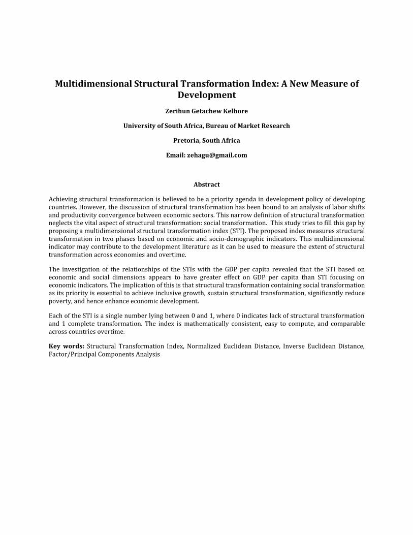
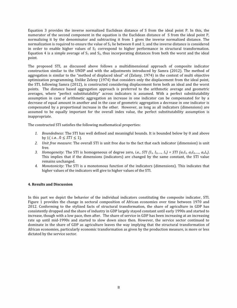
Figure 1 provides the change in sectoral composition of African economies over time between 1970 and

2012. Conforming to the stylized facts of structural transformation, the share of agriculture in GDP has

consistently dropped and the share of industry in GDP largely stayed constant until early 1990s and started to

increase, though with a low pace, then after. The share of service in GDP has been increasing at an increasing

rate up until mid-1990s and started to slow down since then. However, the service sector continued to

dominate in the share of GDP as agriculture leaves the way implying that the structural transformation of

African economies, particularly economic transformation as given by the production measure, is more or less

dictated by the service sector.

9

3.78

3.8

3.82

3.84

Log

of S

ervi

ce V

alue

Add

ed

3.1

3.2

3.3

3.4

3.5

1970 1980 1990 2000 2010Year

Log of Agri. Value Added Log of Industry Value Added

Log of Service Value Added

Figure 1 Change in Sectoral Composition of African Economies overtime, 1970—2012.

Although we have shown the shares of industry in GDP in its broader definition, the contribution of

manufacturing—thought to be the nucleus of the modern economic growth—is dismal as the share of

manufacturing in GDP changed from 10.79% in 1981 to 10.92% in 2010 (WDI, 2014).The dismal

performance of manufacturing over the three decades period implies that the structural transformation in the

economic front has been largely biased towards the service sector. Therefore, the structural transformation

in the economic front, we can say, is not in the conventional direction in which countries move out of

agriculture, embark on industrialization, and end up services dominated. The drift of African countries out of

the conventional path is influenced by stagnation of the growth of the agricultural sector that led to rapid

labor migration to urban informal service sector, which appear to have lower productivity levels. Further, this

labor shift to the informal service sector has been aggravated due to inadequate expansion of the industrial

sector to absorb the growing labor force, and decline in the agricultural sector faster than normal under

successful transformation (Badiane, 2012).

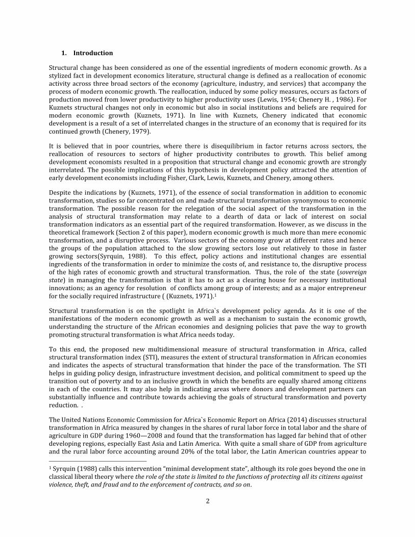
Over the past four decades urbanization in Africa has increased more than two-fold. The rising urbanization

may lead to change in social structure and requires the urbanites to adopt the modern life style of urban

areas. Further, the increasing urban population increases demands of social services commensurate with

urban areas, and this in turn, results in transformation of and widespread of social institutions and expansion

of socio-economic infrastructures such as roads, communication, electricity, and health services.

10

1012

1416

1820

Cru

de D

eath

Rat

e

2025

3035

4045

1970 1980 1990 2000 2010Year

Urbanization Crude Birth Rate

Crude Death Rate

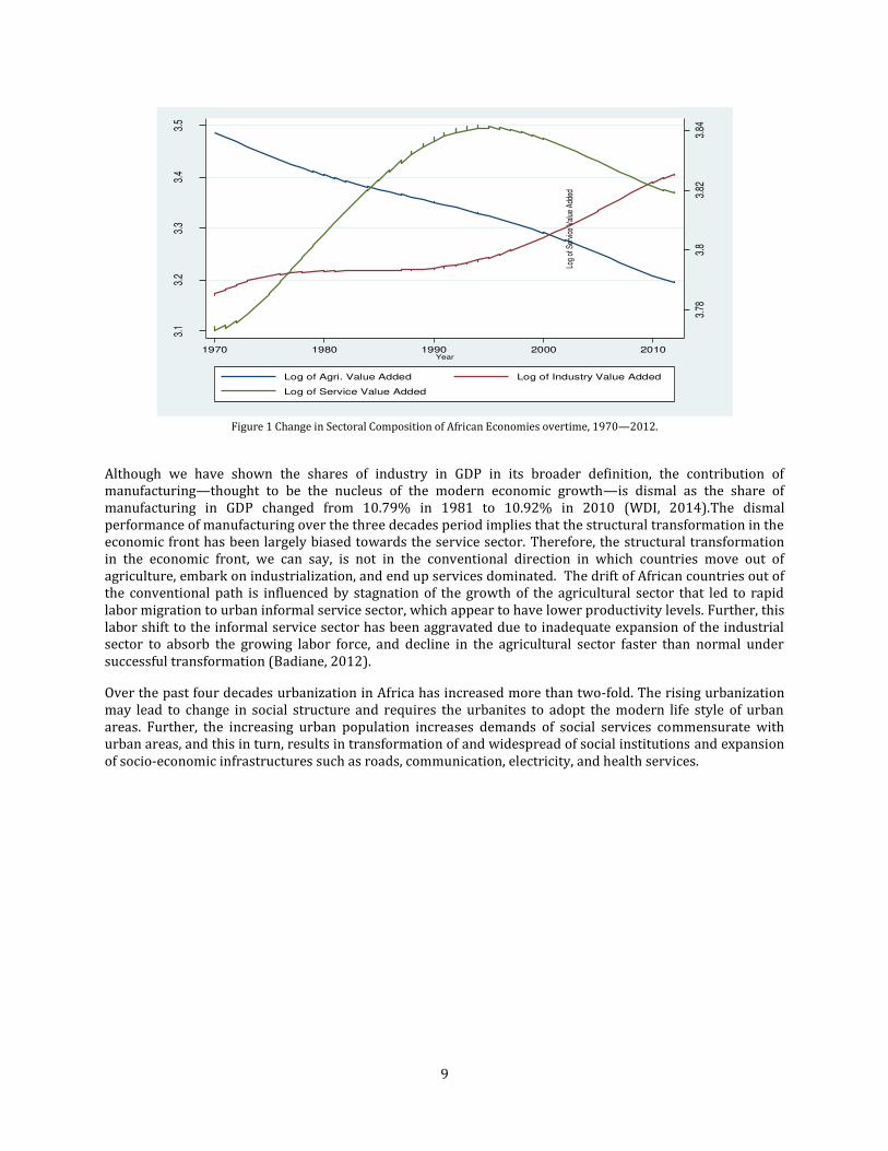
Figure 2 Urbanization and Demographic Transition in Africa, 1970—2012.

The demographic transition indicators (crude birth rate and crude death rates per 1000 people) indicate that

Africa is still in stage two of the demographic transition. The crude death rate per 1000 people substantially

declined from about 20 to 10 over the period of four decades owing to the application of highly effective

imported medical and public health technologies. Similarly, the crude birth rate per 1000 people has declined

from over 45 to 34. Although, this implies that the stage of the demographic transition in Africa is still marked

by high population growth, the declining rates are indicative of the undergoing demographic transition. The

progress in demographic transition from high fertility and mortality to low fertility and mortality paves the

way for reaping the demographic dividend that follows the transition4.

4.1 Economic Transformation

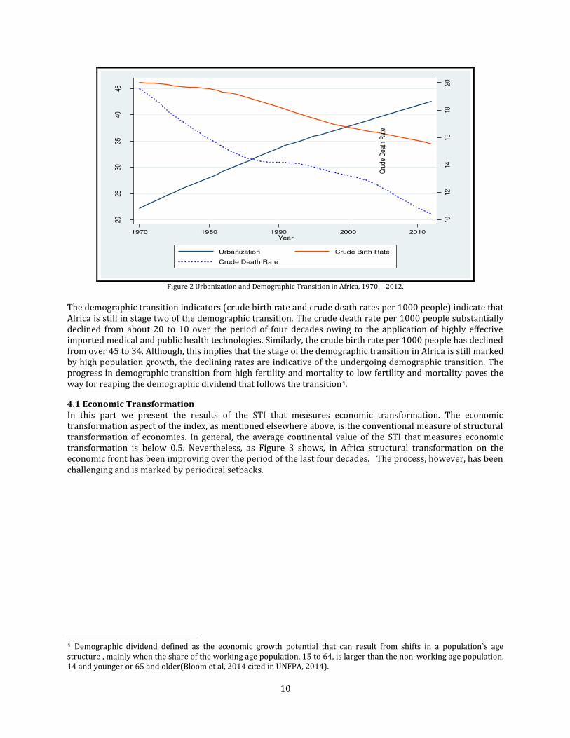
In this part we present the results of the STI that measures economic transformation. The economic

transformation aspect of the index, as mentioned elsewhere above, is the conventional measure of structural

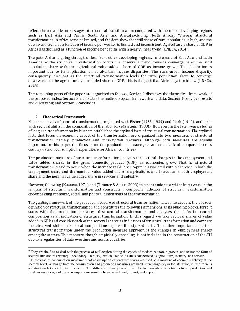
transformation of economies. In general, the average continental value of the STI that measures economic

transformation is below 0.5. Nevertheless, as Figure 3 shows, in Africa structural transformation on the

economic front has been improving over the period of the last four decades. The process, however, has been

challenging and is marked by periodical setbacks.

4 Demographic dividend defined as the economic growth potential that can result from shifts in a population`s age

structure , mainly when the share of the working age population, 15 to 64, is larger than the non-working age population,

14 and younger or 65 and older(Bloom et al, 2014 cited in UNFPA, 2014).

11

.22

.24

.26

.28

.3.3

2

1970 1980 1990 2000 2010

Year

Figure 3 STI (Economic) for Africa from 1970—2012

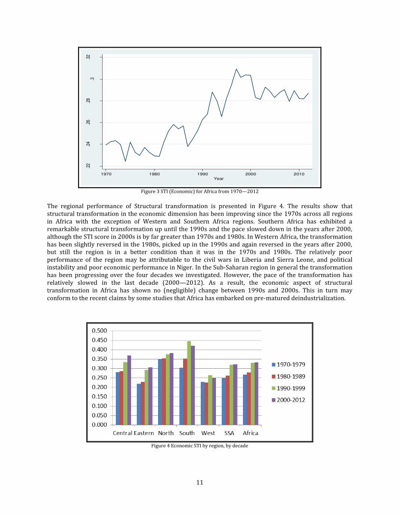
The regional performance of Structural transformation is presented in Figure 4. The results show that

structural transformation in the economic dimension has been improving since the 1970s across all regions

in Africa with the exception of Western and Southern Africa regions. Southern Africa has exhibited a

remarkable structural transformation up until the 1990s and the pace slowed down in the years after 2000,

although the STI score in 2000s is by far greater than 1970s and 1980s. In Western Africa, the transformation

has been slightly reversed in the 1980s, picked up in the 1990s and again reversed in the years after 2000,

but still the region is in a better condition than it was in the 1970s and 1980s. The relatively poor

performance of the region may be attributable to the civil wars in Liberia and Sierra Leone, and political

instability and poor economic performance in Niger. In the Sub-Saharan region in general the transformation

has been progressing over the four decades we investigated. However, the pace of the transformation has

relatively slowed in the last decade (2000—2012). As a result, the economic aspect of structural

transformation in Africa has shown no (negligible) change between 1990s and 2000s. This in turn may

conform to the recent claims by some studies that Africa has embarked on pre-matured deindustrialization.

Figure 4 Economic STI by region, by decade

12

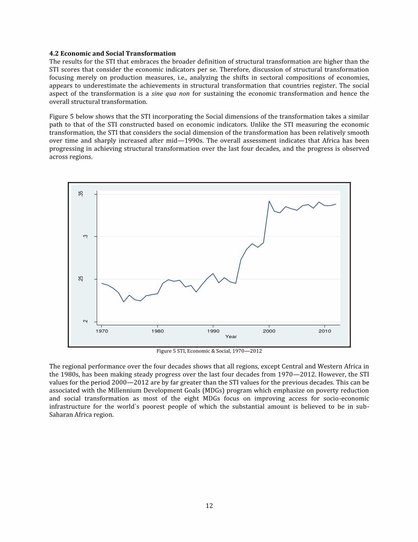
4.2 Economic and Social Transformation

The results for the STI that embraces the broader definition of structural transformation are higher than the

STI scores that consider the economic indicators per se. Therefore, discussion of structural transformation

focusing merely on production measures, i.e., analyzing the shifts in sectoral compositions of economies,

appears to underestimate the achievements in structural transformation that countries register. The social

aspect of the transformation is a sine qua non for sustaining the economic transformation and hence the

overall structural transformation.

Figure 5 below shows that the STI incorporating the Social dimensions of the transformation takes a similar

path to that of the STI constructed based on economic indicators. Unlike the STI measuring the economic

transformation, the STI that considers the social dimension of the transformation has been relatively smooth

over time and sharply increased after mid—1990s. The overall assessment indicates that Africa has been

progressing in achieving structural transformation over the last four decades, and the progress is observed

across regions.

.35

.25

.2.3

1970 1980 1990 2000 2010

Year

Figure 5 STI, Economic & Social, 1970—2012

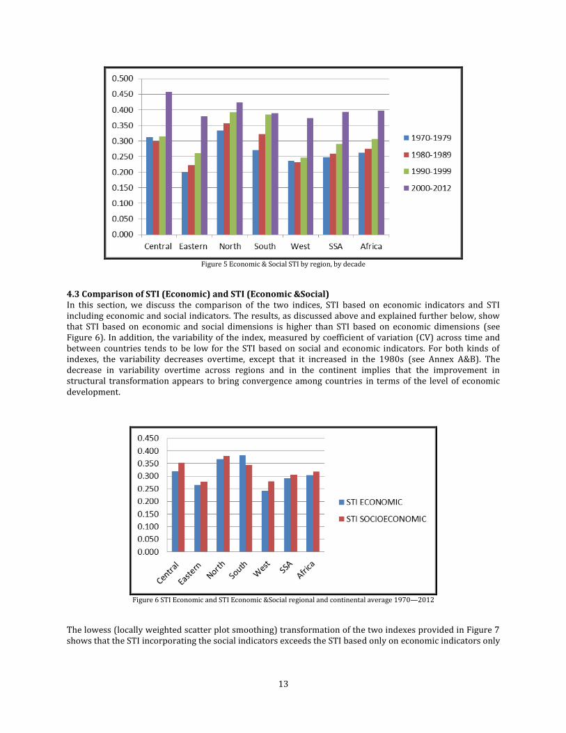
The regional performance over the four decades shows that all regions, except Central and Western Africa in

the 1980s, has been making steady progress over the last four decades from 1970—2012. However, the STI

values for the period 2000—2012 are by far greater than the STI values for the previous decades. This can be

associated with the Millennium Development Goals (MDGs) program which emphasize on poverty reduction

and social transformation as most of the eight MDGs focus on improving access for socio-economic

infrastructure for the world`s poorest people of which the substantial amount is believed to be in sub-

Saharan Africa region.

13

Figure 5 Economic & Social STI by region, by decade

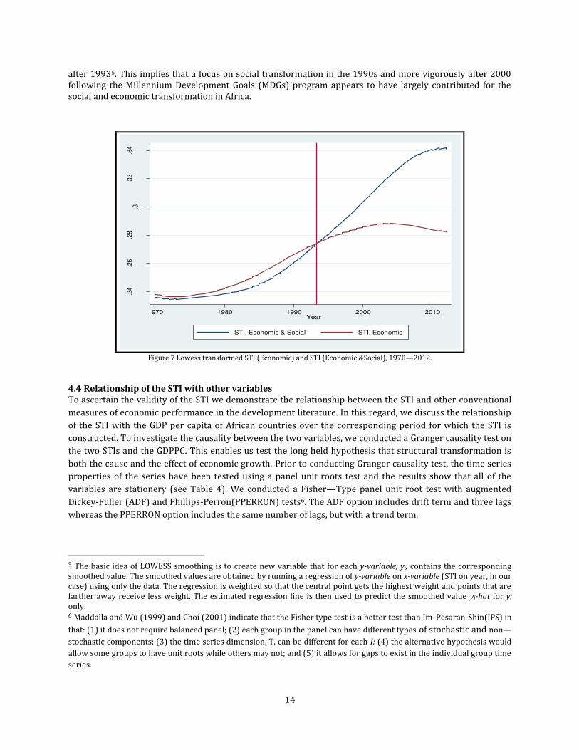
4.3 Comparison of STI (Economic) and STI (Economic &Social)

In this section, we discuss the comparison of the two indices, STI based on economic indicators and STI

including economic and social indicators. The results, as discussed above and explained further below, show

that STI based on economic and social dimensions is higher than STI based on economic dimensions (see

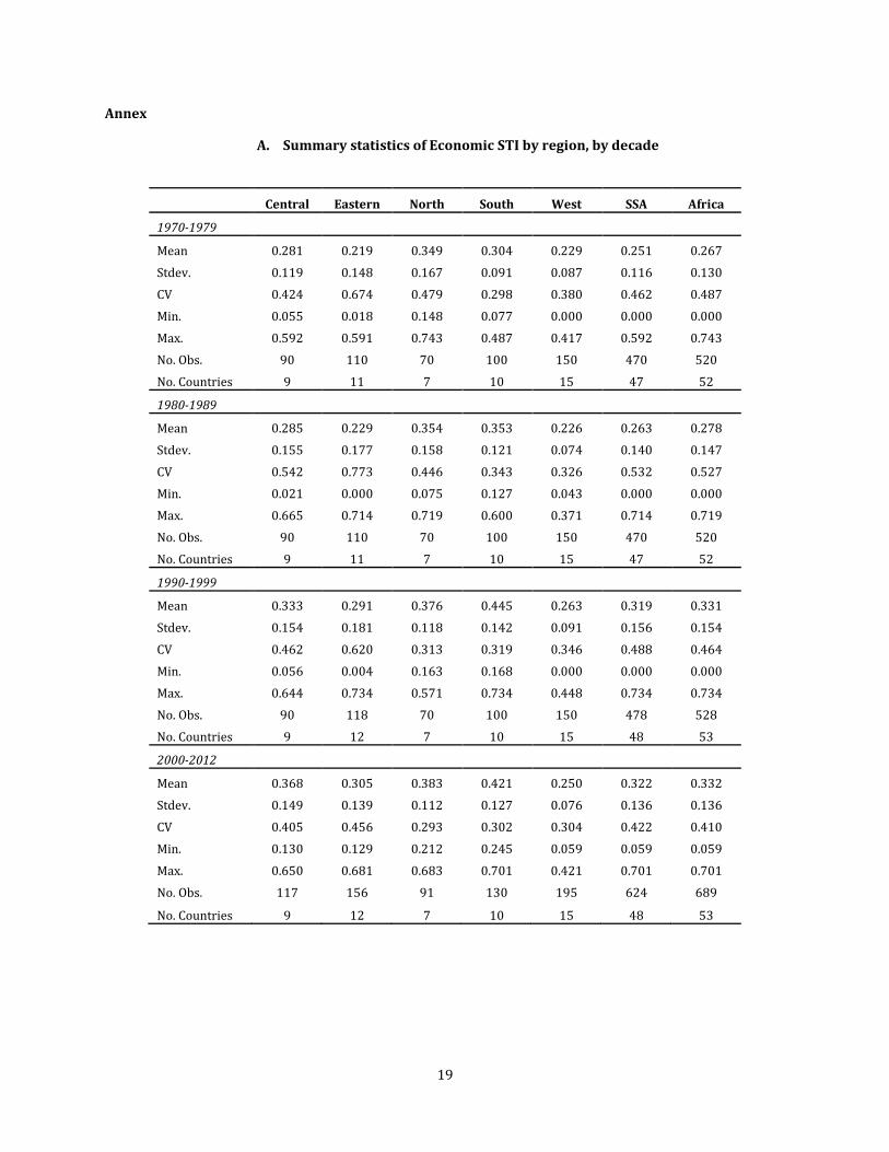
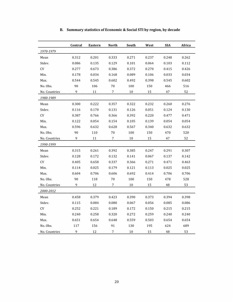
Figure 6). In addition, the variability of the index, measured by coefficient of variation (CV) across time and

between countries tends to be low for the STI based on social and economic indicators. For both kinds of

indexes, the variability decreases overtime, except that it increased in the 1980s (see Annex A&B). The

decrease in variability overtime across regions and in the continent implies that the improvement in

structural transformation appears to bring convergence among countries in terms of the level of economic

development.

Figure 6 STI Economic and STI Economic &Social regional and continental average 1970—2012

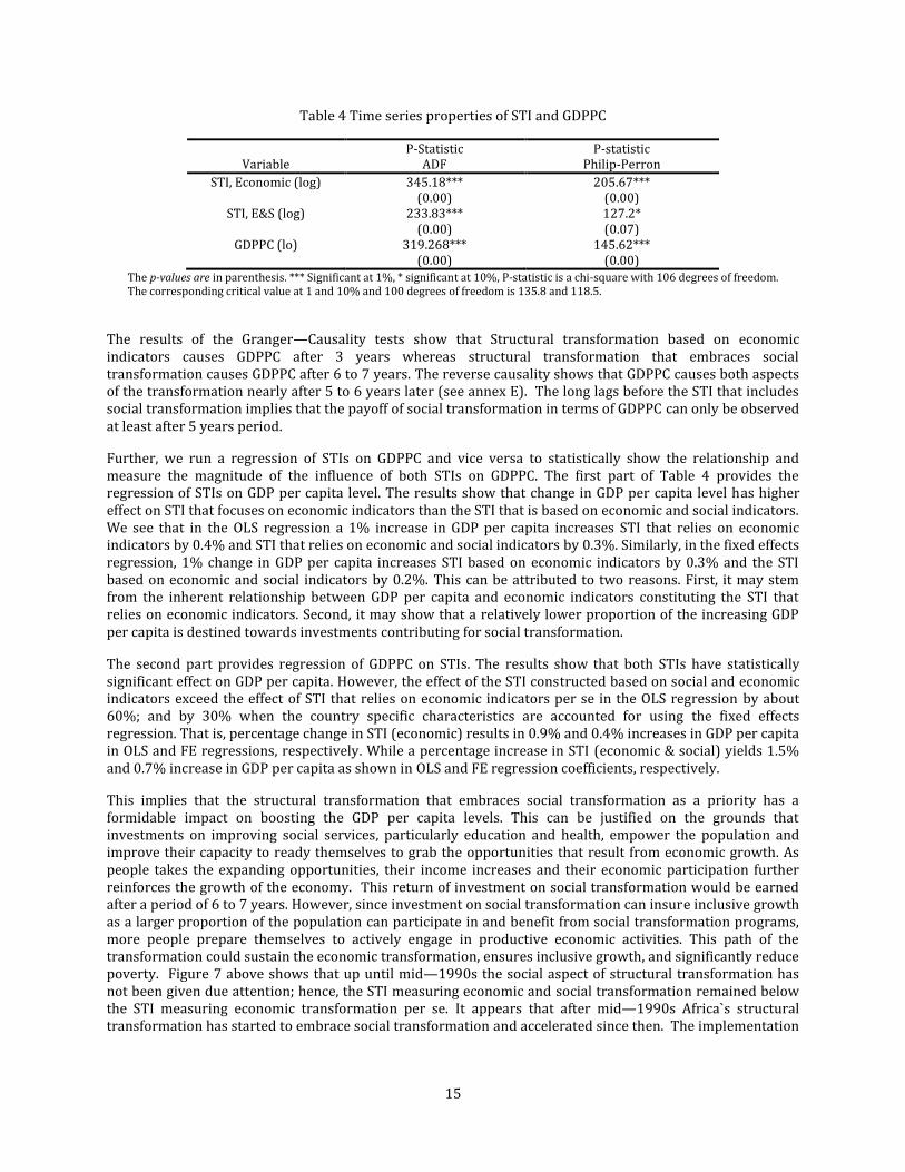
The lowess (locally weighted scatter plot smoothing) transformation of the two indexes provided in Figure 7

shows that the STI incorporating the social indicators exceeds the STI based only on economic indicators only

14

after 19935. This implies that a focus on social transformation in the 1990s and more vigorously after 2000

following the Millennium Development Goals (MDGs) program appears to have largely contributed for the

social and economic transformation in Africa.

.24

.26

.28

.3.3

2.3

4

1970 1980 1990 2000 2010Year

STI, Economic & Social STI, Economic

Figure 7 Lowess transformed STI (Economic) and STI (Economic &Social), 1970—2012.

4.4 Relationship of the STI with other variables

To ascertain the validity of the STI we demonstrate the relationship between the STI and other conventional

measures of economic performance in the development literature. In this regard, we discuss the relationship

of the STI with the GDP per capita of African countries over the corresponding period for which the STI is

constructed. To investigate the causality between the two variables, we conducted a Granger causality test on

the two STIs and the GDPPC. This enables us test the long held hypothesis that structural transformation is

both the cause and the effect of economic growth. Prior to conducting Granger causality test, the time series

properties of the series have been tested using a panel unit roots test and the results show that all of the

variables are stationery (see Table 4). We conducted a Fisher—Type panel unit root test with augmented

Dickey-Fuller (ADF) and Phillips-Perron(PPERRON) tests6. The ADF option includes drift term and three lags

whereas the PPERRON option includes the same number of lags, but with a trend term.

5 The basic idea of LOWESS smoothing is to create new variable that for each y-variable, yi, contains the corresponding

smoothed value. The smoothed values are obtained by running a regression of y-variable on x-variable (STI on year, in our

case) using only the data. The regression is weighted so that the central point gets the highest weight and points that are

farther away receive less weight. The estimated regression line is then used to predict the smoothed value yi-hat for yi

only. 6 Maddalla and Wu (1999) and Choi (2001) indicate that the Fisher type test is a better test than Im-Pesaran-Shin(IPS) in

that: (1) it does not require balanced panel; (2) each group in the panel can have different types of stochastic and non—stochastic components; (3) the time series dimension, T, can be different for each I; (4) the alternative hypothesis would

allow some groups to have unit roots while others may not; and (5) it allows for gaps to exist in the individual group time

series.

15

Table 4 Time series properties of STI and GDPPC

Variable

P-Statistic

ADF

P-statistic

Philip-Perron

STI, Economic (log)

345.18***

(0.00)

205.67***

(0.00)

STI, E&S (log)

233.83***

(0.00)

127.2*

(0.07)

GDPPC (lo)

319.268***

(0.00)

145.62***

(0.00)

The p-values are in parenthesis. *** Significant at 1%, * significant at 10%, P-statistic is a chi-square with 106 degrees of freedom.

The corresponding critical value at 1 and 10% and 100 degrees of freedom is 135.8 and 118.5.

The results of the Granger—Causality tests show that Structural transformation based on economic

indicators causes GDPPC after 3 years whereas structural transformation that embraces social

transformation causes GDPPC after 6 to 7 years. The reverse causality shows that GDPPC causes both aspects

of the transformation nearly after 5 to 6 years later (see annex E). The long lags before the STI that includes

social transformation implies that the payoff of social transformation in terms of GDPPC can only be observed

at least after 5 years period.

Further, we run a regression of STIs on GDPPC and vice versa to statistically show the relationship and

measure the magnitude of the influence of both STIs on GDPPC. The first part of Table 4 provides the

regression of STIs on GDP per capita level. The results show that change in GDP per capita level has higher

effect on STI that focuses on economic indicators than the STI that is based on economic and social indicators.

We see that in the OLS regression a 1% increase in GDP per capita increases STI that relies on economic

indicators by 0.4% and STI that relies on economic and social indicators by 0.3%. Similarly, in the fixed effects

regression, 1% change in GDP per capita increases STI based on economic indicators by 0.3% and the STI

based on economic and social indicators by 0.2%. This can be attributed to two reasons. First, it may stem

from the inherent relationship between GDP per capita and economic indicators constituting the STI that

relies on economic indicators. Second, it may show that a relatively lower proportion of the increasing GDP

per capita is destined towards investments contributing for social transformation.

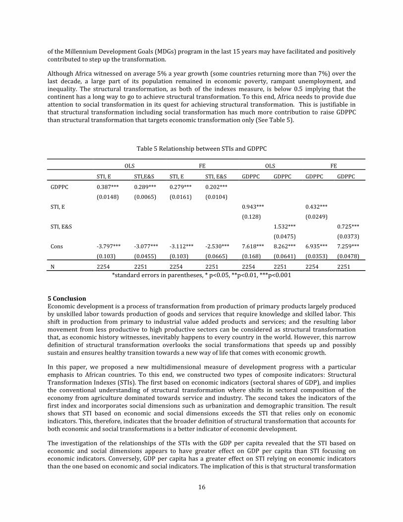
The second part provides regression of GDPPC on STIs. The results show that both STIs have statistically

significant effect on GDP per capita. However, the effect of the STI constructed based on social and economic

indicators exceed the effect of STI that relies on economic indicators per se in the OLS regression by about

60%; and by 30% when the country specific characteristics are accounted for using the fixed effects

regression. That is, percentage change in STI (economic) results in 0.9% and 0.4% increases in GDP per capita

in OLS and FE regressions, respectively. While a percentage increase in STI (economic & social) yields 1.5%

and 0.7% increase in GDP per capita as shown in OLS and FE regression coefficients, respectively.

This implies that the structural transformation that embraces social transformation as a priority has a

formidable impact on boosting the GDP per capita levels. This can be justified on the grounds that

investments on improving social services, particularly education and health, empower the population and

improve their capacity to ready themselves to grab the opportunities that result from economic growth. As

people takes the expanding opportunities, their income increases and their economic participation further

reinforces the growth of the economy. This return of investment on social transformation would be earned

after a period of 6 to 7 years. However, since investment on social transformation can insure inclusive growth

as a larger proportion of the population can participate in and benefit from social transformation programs,

more people prepare themselves to actively engage in productive economic activities. This path of the

transformation could sustain the economic transformation, ensures inclusive growth, and significantly reduce

poverty. Figure 7 above shows that up until mid—1990s the social aspect of structural transformation has

not been given due attention; hence, the STI measuring economic and social transformation remained below

the STI measuring economic transformation per se. It appears that after mid—1990s Africa`s structural

transformation has started to embrace social transformation and accelerated since then. The implementation

16

of the Millennium Development Goals (MDGs) program in the last 15 years may have facilitated and positively

contributed to step up the transformation.

Although Africa witnessed on average 5% a year growth (some countries returning more than 7%) over the

last decade, a large part of its population remained in economic poverty, rampant unemployment, and

inequality. The structural transformation, as both of the indexes measure, is below 0.5 implying that the

continent has a long way to go to achieve structural transformation. To this end, Africa needs to provide due

attention to social transformation in its quest for achieving structural transformation. This is justifiable in

that structural transformation including social transformation has much more contribution to raise GDPPC

than structural transformation that targets economic transformation only (See Table 5).

Table 5 Relationship between STIs and GDPPC

OLS FE OLS FE

STI, E STI,E&S STI, E STI, E&S GDPPC GDPPC GDPPC GDPPC

GDPPC 0.387*** 0.289*** 0.279*** 0.202***

(0.0148) (0.0065) (0.0161) (0.0104)

STI, E

0.943*** 0.432***

(0.128) (0.0249)

STI, E&S

1.532*** 0.725***

(0.0475) (0.0373)

Cons -3.797*** -3.077*** -3.112*** -2.530*** 7.618*** 8.262*** 6.935*** 7.259***

(0.103) (0.0455) (0.103) (0.0665) (0.168) (0.0641) (0.0353) (0.0478)

N 2254 2251 2254 2251 2254 2251 2254 2251

*standard errors in parentheses, * p<0.05, **p<0.01, ***p<0.001

5 Conclusion

Economic development is a process of transformation from production of primary products largely produced

by unskilled labor towards production of goods and services that require knowledge and skilled labor. This

shift in production from primary to industrial value added products and services; and the resulting labor

movement from less productive to high productive sectors can be considered as structural transformation

that, as economic history witnesses, inevitably happens to every country in the world. However, this narrow

definition of structural transformation overlooks the social transformations that speeds up and possibly

sustain and ensures healthy transition towards a new way of life that comes with economic growth.

In this paper, we proposed a new multidimensional measure of development progress with a particular

emphasis to African countries. To this end, we constructed two types of composite indicators: Structural

Transformation Indexes (STIs). The first based on economic indicators (sectoral shares of GDP), and implies

the conventional understanding of structural transformation where shifts in sectoral composition of the

economy from agriculture dominated towards service and industry. The second takes the indicators of the

first index and incorporates social dimensions such as urbanization and demographic transition. The result

shows that STI based on economic and social dimensions exceeds the STI that relies only on economic

indicators. This, therefore, indicates that the broader definition of structural transformation that accounts for

both economic and social transformations is a better indicator of economic development.

The investigation of the relationships of the STIs with the GDP per capita revealed that the STI based on

economic and social dimensions appears to have greater effect on GDP per capita than STI focusing on

economic indicators. Conversely, GDP per capita has a greater effect on STI relying on economic indicators

than the one based on economic and social indicators. The implication of this is that structural transformation

17

incorporating social transformation is important to achieve solid and sustainable structural transformation

and hence inclusive economic growth and development. Most importantly, it significantly contributes to

poverty reduction as the social transformation involves more population and allows them to ready

themselves both to take up economic opportunities and maintain the economic growth.

Thus, in order to achieve inclusive economic development African countries must provide due attention to

achieving social transformation. To this effect, designing policies and strategies that focus on improving

education, health, and physical infrastructure is a priority and has to be done juxtaposed to other investments

that help in fostering economic transformation such as industrialization.

18

References

Badiane, O. (2012). Beyond Economic Recovery: The Agenda for Economic Transformation in Africa, in Patterns

of Economic Growth and Structural Transformation in Africa . IFPRI. Washington D.C.: International

Food Policy Research Institute.

Chenery, H. (1979). Structural Change and Development Policy. New York: Oxford University Press.

Chenery, H. (1986). Growth and Transformation, in: H. Chenery, S. Robinson and M. Syrquin, Industrialization

and Growth. New York: Oxford University Press.

Choi, I. (2001). Unit Root Tests for Panel Data. Journal of International Money and Finance, 20, 249-272.

Kuznets, S. (1971). Economic Growth oof Nations. Cambridge, MA: Harvard University Press.

Lewis, W. A. (1954). Economic Development with unlimited supplies of labor. Manchester School of Economic

and Social Studies.

Madalla, G., & Wu, S. (1999). A Comparative Study of Unit Root Tests with Panel Data an New Simple Test.

Oxford Bulletin of Economics and Statistics(Special Issue), 0305-0349.

UNFPA. (2014). The Power of 1.8 Billion: Adolescents, Youth, and the Transformation of the Future: The State of

World Population in 2014. New York: United Nations Population Fund.

Hammond, A., Adriaanse, A., Rodenburg, E., Bryant, D., & Woodward, R. (1995). Environmental indicators: A

systematic approach to measuring and reporting on environmental policy performance in the context of

sustainable development (Vol. 36, p. 460). World Resource Institute.

OECD. (2008). Handbook on Constructing Composite Indicators (pp. 1–162). Paris: OECD Publishing.

Saltelli, A. (2007). Composite indicators between analysis and advocacy. Social Indicators Research, 81, 65–77.

doi:10.1007/s11205-006-0024-9

Sarma, M. (2012). Index of Financial Inclusion – A measure of financial sector inclusiveness Mandira Sarma July

2012 (No. 07). Berlin.

Syrquin, M. (1988). Chapter 7 Patterns of structural change. Handbook of Development Economics, 1, 203–273.

doi:10.1016/S1573-4471(88)01010-1

Timmer, B. C. P., & Akkus, S. (2008). The Structural Transformation as a Pathway out of Poverty : Analytics , Empirics and Politics. Center for Global Development, (150).

UNECA. (2014). Ecopnomic Report on Africa: Dynamic industrial policy in africa. Addis Ababa, Ethiopia: United

Nations Economic Commission for Africa.

Zelany, M. (1974). A concept of compromise solutions and the method of the displaced ideal. Computers &

Operations Research, 1, 479–496. doi:10.1016/0305-0548(74)90064-1

19

Annex

A. Summary statistics of Economic STI by region, by decade

Central Eastern North South West SSA Africa

1970-1979

Mean 0.281 0.219 0.349 0.304 0.229 0.251 0.267

Stdev. 0.119 0.148 0.167 0.091 0.087 0.116 0.130

CV 0.424 0.674 0.479 0.298 0.380 0.462 0.487

Min. 0.055 0.018 0.148 0.077 0.000 0.000 0.000

Max. 0.592 0.591 0.743 0.487 0.417 0.592 0.743

No. Obs. 90 110 70 100 150 470 520

No. Countries 9 11 7 10 15 47 52

1980-1989

Mean 0.285 0.229 0.354 0.353 0.226 0.263 0.278

Stdev. 0.155 0.177 0.158 0.121 0.074 0.140 0.147

CV 0.542 0.773 0.446 0.343 0.326 0.532 0.527

Min. 0.021 0.000 0.075 0.127 0.043 0.000 0.000

Max. 0.665 0.714 0.719 0.600 0.371 0.714 0.719

No. Obs. 90 110 70 100 150 470 520

No. Countries 9 11 7 10 15 47 52

1990-1999

Mean 0.333 0.291 0.376 0.445 0.263 0.319 0.331

Stdev. 0.154 0.181 0.118 0.142 0.091 0.156 0.154

CV 0.462 0.620 0.313 0.319 0.346 0.488 0.464

Min. 0.056 0.004 0.163 0.168 0.000 0.000 0.000

Max. 0.644 0.734 0.571 0.734 0.448 0.734 0.734

No. Obs. 90 118 70 100 150 478 528

No. Countries 9 12 7 10 15 48 53

2000-2012

Mean 0.368 0.305 0.383 0.421 0.250 0.322 0.332

Stdev. 0.149 0.139 0.112 0.127 0.076 0.136 0.136

CV 0.405 0.456 0.293 0.302 0.304 0.422 0.410

Min. 0.130 0.129 0.212 0.245 0.059 0.059 0.059

Max. 0.650 0.681 0.683 0.701 0.421 0.701 0.701

No. Obs. 117 156 91 130 195 624 689

No. Countries 9 12 7 10 15 48 53

20

B. Summary statistics of Economic & Social STI by region, by decade

Central Eastern North South West SSA Africa

1970-1979

Mean 0.312 0.201 0.333 0.271 0.237 0.248 0.262

Stdev. 0.086 0.135 0.129 0.101 0.064 0.103 0.112

CV 0.277 0.673 0.386 0.372 0.270 0.415 0.426

Min. 0.178 0.034 0.168 0.089 0.106 0.033 0.034

Max. 0.544 0.545 0.602 0.492 0.398 0.545 0.602

No. Obs. 90 106 70 100 150 466 516

No. Countries 9 11 7 10 15 47 52

1980-1989

Mean 0.300 0.222 0.357 0.322 0.232 0.260 0.276

Stdev. 0.116 0.170 0.131 0.126 0.051 0.124 0.130

CV 0.387 0.766 0.366 0.392 0.220 0.477 0.471

Min. 0.122 0.054 0.154 0.105 0.139 0.054 0.054

Max. 0.596 0.632 0.628 0.567 0.340 0.632 0.632

No. Obs. 90 110 70 100 150 470 520

No. Countries 9 11 7 10 15 47 52

1990-1999

Mean 0.315 0.261 0.392 0.385 0.247 0.291 0.307

Stdev. 0.128 0.172 0.132 0.141 0.067 0.137 0.142

CV 0.405 0.658 0.337 0.366 0.271 0.471 0.463

Min. 0.114 0.025 0.179 0.121 0.113 0.025 0.025

Max. 0.604 0.706 0.606 0.692 0.414 0.706 0.706

No. Obs. 90 118 70 100 150 478 528

No. Countries 9 12 7 10 15 48 53

2000-2012

Mean 0.458 0.379 0.423 0.390 0.373 0.394 0.398

Stdev. 0.115 0.084 0.080 0.067 0.056 0.085 0.086

CV 0.252 0.221 0.189 0.172 0.150 0.215 0.215

Min. 0.240 0.258 0.320 0.272 0.259 0.240 0.240

Max. 0.651 0.654 0.648 0.559 0.503 0.654 0.654

No. Obs. 117 156 91 130 195 624 689

No. Countries 9 12 7 10 15 48 53

21

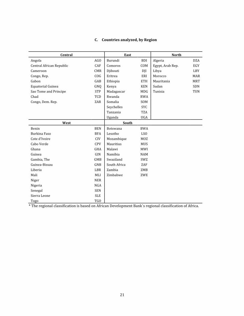
C. Countries analyzed, by Region

Central East North

Angola AGO Burundi BDI Algeria DZA

Central African Republic CAF Comoros COM Egypt, Arab Rep. EGY

Cameroon CMR Djibouti DJI Libya LBY

Congo, Rep. COG Eritrea ERI Morocco MAR

Gabon GAB Ethiopia ETH Mauritania MRT

Equatorial Guinea GNQ Kenya KEN Sudan SDN

Sao Tome and Principe STP Madagascar MDG Tunisia TUN

Chad TCD Rwanda RWA

Congo, Dem. Rep. ZAR Somalia SOM

Seychelles SYC

Tanzania TZA

Uganda UGA

West South

Benin BEN Botswana BWA

Burkina Faso BFA Lesotho LSO

Cote d'Ivoire CIV Mozambique MOZ

Cabo Verde CPV Mauritius MUS

Ghana GHA Malawi MWI

Guinea GIN Namibia NAM

Gambia, The GMB Swaziland SWZ

Guinea-Bissau GNB South Africa ZAF

Liberia LBR Zambia ZMB

Mali MLI Zimbabwe ZWE

Niger NER

Nigeria NGA

Senegal SEN

Sierra Leone SLE

Togo TGO

* The regional classification is based on African Development Bank`s regional classification of Africa.

22

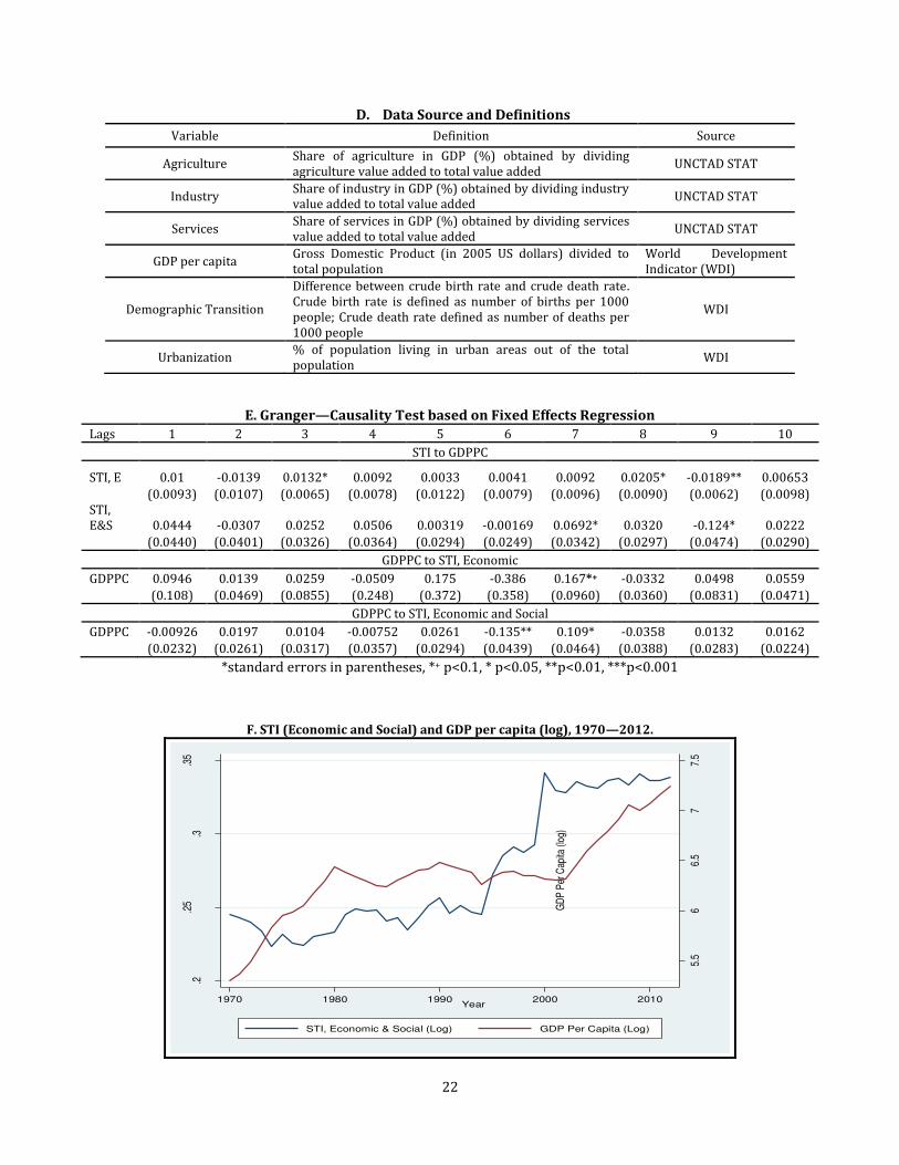
D. Data Source and Definitions

Variable Definition Source

Agriculture Share of agriculture in GDP (%) obtained by dividing

agriculture value added to total value added UNCTAD STAT

Industry Share of industry in GDP (%) obtained by dividing industry

value added to total value added UNCTAD STAT

Services Share of services in GDP (%) obtained by dividing services

value added to total value added UNCTAD STAT

GDP per capita Gross Domestic Product (in 2005 US dollars) divided to

total population

World Development

Indicator (WDI)

Demographic Transition

Difference between crude birth rate and crude death rate.

Crude birth rate is defined as number of births per 1000

people; Crude death rate defined as number of deaths per

1000 people

WDI

Urbanization % of population living in urban areas out of the total

population WDI

E. Granger—Causality Test based on Fixed Effects Regression

Lags 1 2 3 4 5 6 7 8 9 10

STI to GDPPC

STI, E 0.01 -0.0139 0.0132* 0.0092 0.0033 0.0041 0.0092 0.0205* -0.0189** 0.00653

(0.0093) (0.0107) (0.0065) (0.0078) (0.0122) (0.0079) (0.0096) (0.0090) (0.0062) (0.0098)

STI,

E&S 0.0444 -0.0307 0.0252 0.0506 0.00319 -0.00169 0.0692* 0.0320 -0.124* 0.0222

(0.0440) (0.0401) (0.0326) (0.0364) (0.0294) (0.0249) (0.0342) (0.0297) (0.0474) (0.0290)

GDPPC to STI, Economic

GDPPC 0.0946 0.0139 0.0259 -0.0509 0.175 -0.386 0.167*+ -0.0332 0.0498 0.0559

(0.108) (0.0469) (0.0855) (0.248) (0.372) (0.358) (0.0960) (0.0360) (0.0831) (0.0471)

GDPPC to STI, Economic and Social

GDPPC -0.00926 0.0197 0.0104 -0.00752 0.0261 -0.135** 0.109* -0.0358 0.0132 0.0162

(0.0232) (0.0261) (0.0317) (0.0357) (0.0294) (0.0439) (0.0464) (0.0388) (0.0283) (0.0224)

*standard errors in parentheses, *+ p<0.1, * p<0.05, **p<0.01, ***p<0.001

F. STI (Economic and Social) and GDP per capita (log), 1970—2012.

5.5

66.

57

7.5

GD

P P

er C

apita

(log

)

.2.2

5.3

.35

1970 1980 1990 2000 2010Year

STI, Economic & Social (Log) GDP Per Capita (Log)