Research Division Federal Reserve Bank of St. Louis Working Paper Series

Rural-Urban Migration, Structural Transformation, and Housing Markets in China

Carlos Garriga Yang Tang

And Ping Wang

Working Paper 2014-028C http://research.stlouisfed.org/wp/2014/2014-028.pdf

April 21, 2016

FEDERAL RESERVE BANK OF ST. LOUIS Research Division

P.O. Box 442 St. Louis, MO 63166

______________________________________________________________________________________

The views expressed are those of the individual authors and do not necessarily reflect official positions of the Federal Reserve Bank of St. Louis, the Federal Reserve System, or the Board of Governors.

Federal Reserve Bank of St. Louis Working Papers are preliminary materials circulated to stimulate discussion and critical comment. References in publications to Federal Reserve Bank of St. Louis Working Papers (other than an acknowledgment that the writer has had access to unpublished material) should be cleared with the author or authors.

Rural-Urban Migration, Structural Transformation,and Housing Markets in China

Carlos GarrigaFederal Reserve Bank of St. Louis

Yang TangNanyang Technological University

Ping WangWashington University in St. Louis,

Federal Reserve Bank of St. Louis, and NBER

April 21, 2016

Abstract: This paper explores the contribution of the structural transformation and urban-ization process in the housing market in China. City migration flows combined with aninelastic land supply, due to entry restrictions, has raised house prices. This issue is ex-amined using a multi-sector dynamic general-equilibrium model with migration and housingmarket. Our quantitative findings suggest that this process accounts for about 80 percent ofurban housing prices. This mechanism remains valid in an extension calibrated to the twolargest cities where housing booms have been particularly noticeable. Overall, supply factorsand productivity account for most of the housing price growth.Keywords: Migration, structural transformation, housing boom.JEL Classification: D90, E20, O41, R23, R31.

Acknowledgment: The authors are grateful for stimulating discussions with Costas Azariadis, RickBond, James Bullard, Kaiji Chen, Morris Davis, Jang-Ting Guo, Berthold Herrendorf, Tom Holmes,Alexander Monge-Naranjo, Yongs Shin, Don Schlagenhauf, B. Ravikumar, Paul Romer, MichaelSpence, Stijn Van Nieuwerburgh, Yi Wen, and the seminar participants at the Federal Reserve Bankof St. Louis, Fengchia University, Nanyang Technological University, National Chengchi University,National University of Singapore, Washington University in St. Louis, the 2015 China EconomicsSummer Institute, the 2013 Econometric Society Asia Meeting, the 2015 International Real EstateConference in Singapore, the 2013 Midwest Economic Association Meeting, the 2014 Society forEconomic Dynamics Meeting, the NBER conference on the Chinese Economy, the 6th ShanghaiMacroeconomic Workshop, and the 2015 Meetings of Society for the Advancement of EconomicTheory. The views expressed herein do not necessarily reflect those of the Federal Reserve Bank ofSt. Louis, the Board of Governors, or the Federal Reserve System.Correspondence: Ping Wang, Department of Economics, Washington University in St. Louis, St.Louis, MO 63130, U.S.A.; 314-935-4236 (Phone): 314-935-4156 (Fax); pingwang@wustl.edu .

1 Introduction

Over the past three decades, several major developed and developing economies have experi-

enced sizable housing booms over prolonged periods. China – the world’s factory– is one of

the most prominent cases of rapid growth. It has experienced a fast but still ongoing struc-

tural transformation from a largely agricultural society to a modern one whose agricultural

employment share was reduced from almost 70 percent in 1980 to about 33 percent in 2012.

Compared with the speed of its structural transformation, China’s urbanization process has

been relatively moderate, with the rural population dropping from about three-quarters to

still more than half over the same period. Given this moderate urbanization pace, it is to

some degree puzzling why China has experienced one of the most noticeable price hike’s in

urban housing markets, leading its government to implement regulatory mortgage and sales

policies to cool off the housing boom even after the financial tsunami.1 The primary purpose

of this paper is to investigate this issue by exploring the role structural transformation played

in China’s housing boom.

We highlight three major channels through which structural change may have affected

housing prices. First, structural transformation increases manufacturing productivity and

that generates higher incomes in urban areas and a greater ability to pay for housing. Second,

the housing supply is relatively inelastic due to heavy regulations on land supply and the

market entrance of real estate developers. As a consequence of structural transformation,

the third channel is an ongoing rural-urban migration that increases the demand for urban

housing. Our view is that structural transformation implies job reallocation from agricultural

to non-agricultural sectors and also induces migration from rural to urban areas where most

production takes place.

The appreciation of housing values has been remarkable in China. Figure 1 shows the

average real housing price per square meter in China has increased rapidly from about 750

RMB in 1998 to 5000 RMB in 2012. To motivate the main mechanism in our paper, we further

report cross-city data of structural transformation, migration flows, and housing prices in

Figure 2. The top panel plots the average annual growth rate of housing prices against the

average annual growth rate of net migration from rural areas to China’s 29 major cities from

1998-2007.2 The positive relationship suggests that housing prices grow faster in cities with

larger net inflows of migrants from rural areas. The bottom panel plots the average annual

growth rate of the employment share in the non-agricultural sector against the average annual

1Based on the 2000 census, about 87 percent of Chinese households owned houses. According to theNational Bureau of Statistics of China, the total residential investment in urban areas reached nearly 57.8trillion RMB in 2012, which is 100 times more than it was in 1998. The rising demands have led to a surgein housing prices (as documented below).

2This list includes all the first-tier and major second-tier cities in China.

1

growth rate of migration from rural areas to the 29 cities. The positive relationship implies

most migrants from rural areas work in the non-agricultural sector in the cities. These two

observations together are consistent with the idea that workers migrating from rural areas

to cities most likely have switched from agricultural to non-agricultural jobs. As such, cities

offering more non-agricultural jobs can potentially attract more migrants, which in turn can

lead to faster housing price growth rates.

In order to fully examine the influence of structural transformation on urban housing

development, we construct a dynamic general equilibrium model with structural transforma-

tion and endogenous migration. Specifically, we consider an economy that is geographically

divided into two regions: a rural area that produces agricultural goods and an urban area

(a city) that produces manufactured goods (inclusive of urban services in the remainder of

the paper). Ongoing technological progress drives workers away from the rural agricultural

sector to the urban manufacturing sector. When workers arrive in a city, they must purchase

a house with a down payment and a long-term mortgage. In the baseline model, while a

house is required for urban living, it has no resale value. New homes are built by real estate

developers who purchase land and construction permits from the government.

Our basic framework considers only a single urban area and then it is generalized to

multiple cities. This extension allows us to assess the contribution of different migration flows

to changes in housing price growth rates across cities. More importantly, evaluating what

contributed to the structural transformation of large cities further allows us to determine

whether or not any portion of the appreciation in housing prices is induced by structural

change.

To disentangle the contributions of various underlying forces (housing finance, entry fees,

land supply policy, and the productivity of the manufacturing sector), we calibrate the model

to mimic the early stages of development in China from 1980 to 2012. The future projected

path for China’s structural transformation through 2065 is based on the U.S. experience from

1950 to 1990. We restrict our attention to the period from 1998 to 2012. This is because

China’s pre-1998 housing market was largely controlled by the government and housing prices

were heavily regulated.

The main findings can be summarized as follows. At the national level, the process of

structural change can account for 80.5 percent of housing over 1998-2012 and 86.1 percent

over 1998-2007. More specifically, supply factors account for more than 60 percent of the

changes in housing prices. Productivity (income) accounts for more than one-fifth of the

changes in housing with its contribution rising over time, while access to credit has limited

impact throughout the entire sample period.

In the multiple-city case, the model accounts for 82.8 percent and 60.2 percent of housing

2

price growth in Beijing and Shanghai, respectively. While supply conditions remain crucial,

productivity growth becomes more important in explaining Shanghai’s housing prices. Land

supply becomes more important in explaining Beijing’s housing prices during 2008-2012.

In both cities, the role played by productivity is enhanced during 2008-2012. This finding

suggests that market fundamentals driven by structural transformation remain a key driver

of housing prices. At the micro level, an issue that is frequently noted is the possibility of

the burst of “ghost cities.”3 It is noted, however, that this is not a widespread phenomenon

and refers to low-tier cities often overly built by the government. There is some speculation

whether these cities may experience housing bubbles, but these are not representative of the

major metropolitan areas in China.

The baseline model is extended in several dimensions, including the smoothness of the

volatile migration flows, the consideration of tenant-occupied housing, the adoption of non-

homothetic preferences, the introduction of housing quality and the incorporation of savings,

the consumption valuation of housing, and the investment value of housing. We find that

while these extensions could improve on the predictability of housing price movements in

China, such improvements are either marginal or moderate. Thus, not only does structural

transformation remain an important driver of China’s housing boom, but our baseline frame-

work is also viewed as an adequate benchmark for the purpose of our study.

In summary, by incorporating endogenous rural-urban migration decisions responding to

structural change, we find that the process of relocating workers to cities combined with the

typical stages of economic development can account for a nontrivial portion of the housing

boom in China.

Literature Review

The Chinese economy has undergone many political and economic reforms since 1978. Its

rapid growth has made it the second-largest economy in the world, with especially signifi-

cant growth since 1992. There is a large literature studying the development of China. For

brevity, the reader is referred to Zhu (2012) for an extensive summary of the various stages of

economic development. There is a small but growing literature investigating China’s housing

boom, including research by Chen and Wen (2014), Fang, Gu and Zhou (2014), and Deng,

Gyourko, and Wu (2015). In contrast to this literature, we highlight the structural trans-

formation of the manufacturing sector as a key driver of rural migrants to the cities. There

have been numerous studies on structural transformation using dynamic general equilibrium

models without spatial considerations. For a comprehensive survey, the reader is referred to

Herrendorf, Rogerson, and Valentinyi (2014). Of particular relevance, Hansen and Prescott

3This refers to large urban property developments which have remained mostly unoccupied after theywere built.

3

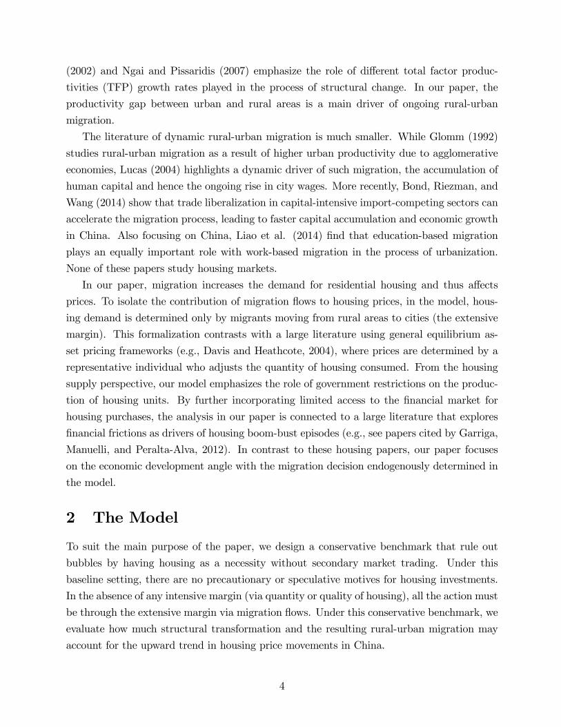
(2002) and Ngai and Pissaridis (2007) emphasize the role of different total factor produc-

tivities (TFP) growth rates played in the process of structural change. In our paper, the

productivity gap between urban and rural areas is a main driver of ongoing rural-urban

migration.

The literature of dynamic rural-urban migration is much smaller. While Glomm (1992)

studies rural-urban migration as a result of higher urban productivity due to agglomerative

economies, Lucas (2004) highlights a dynamic driver of such migration, the accumulation of

human capital and hence the ongoing rise in city wages. More recently, Bond, Riezman, and

Wang (2014) show that trade liberalization in capital-intensive import-competing sectors can

accelerate the migration process, leading to faster capital accumulation and economic growth

in China. Also focusing on China, Liao et al. (2014) find that education-based migration

plays an equally important role with work-based migration in the process of urbanization.

None of these papers study housing markets.

In our paper, migration increases the demand for residential housing and thus affects

prices. To isolate the contribution of migration flows to housing prices, in the model, hous-

ing demand is determined only by migrants moving from rural areas to cities (the extensive

margin). This formalization contrasts with a large literature using general equilibrium as-

set pricing frameworks (e.g., Davis and Heathcote, 2004), where prices are determined by a

representative individual who adjusts the quantity of housing consumed. From the housing

supply perspective, our model emphasizes the role of government restrictions on the produc-

tion of housing units. By further incorporating limited access to the financial market for

housing purchases, the analysis in our paper is connected to a large literature that explores

financial frictions as drivers of housing boom-bust episodes (e.g., see papers cited by Garriga,

Manuelli, and Peralta-Alva, 2012). In contrast to these housing papers, our paper focuses

on the economic development angle with the migration decision endogenously determined in

the model.

2 The Model

To suit the main purpose of the paper, we design a conservative benchmark that rule out

bubbles by having housing as a necessity without secondary market trading. Under this

baseline setting, there are no precautionary or speculative motives for housing investments.

In the absence of any intensive margin (via quantity or quality of housing), all the action must

be through the extensive margin via migration flows. Under this conservative benchmark, we

evaluate how much structural transformation and the resulting rural-urban migration may

account for the upward trend in housing price movements in China.

4

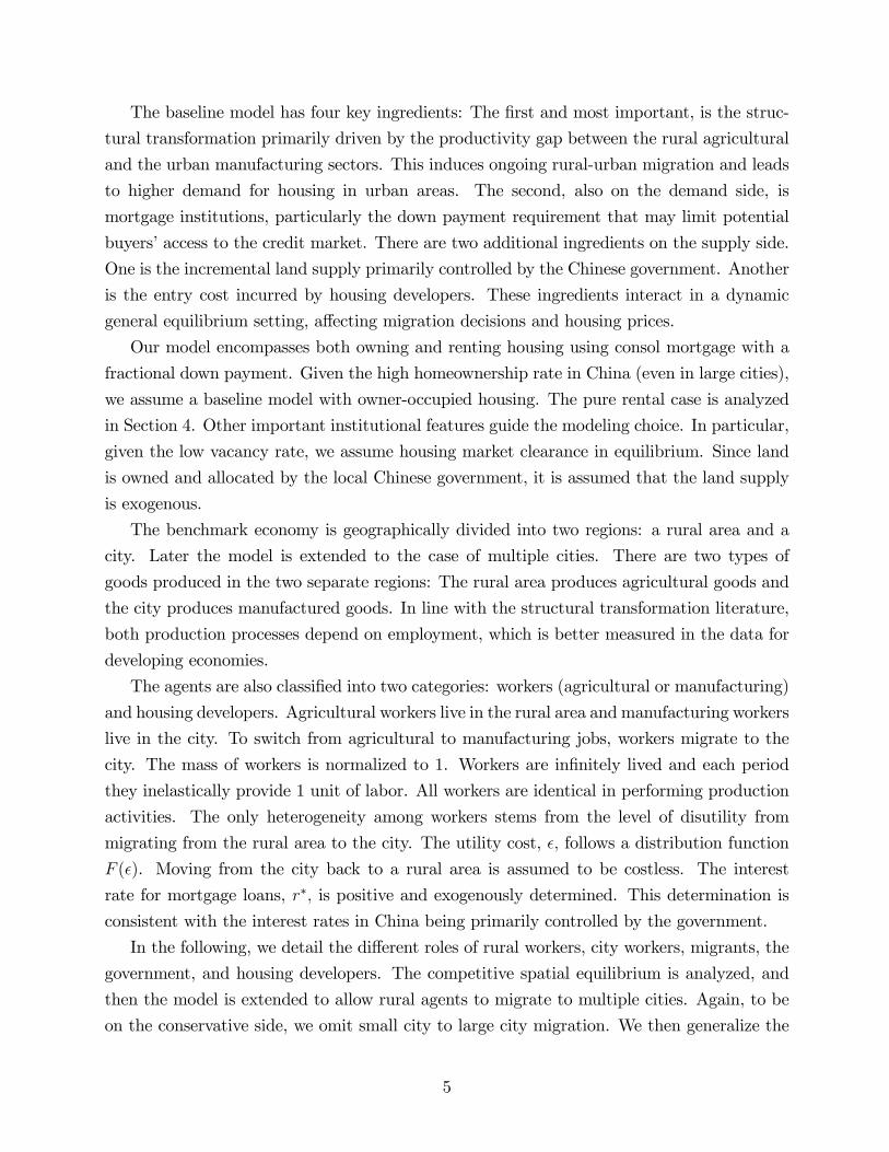
The baseline model has four key ingredients: The first and most important, is the struc-

tural transformation primarily driven by the productivity gap between the rural agricultural

and the urban manufacturing sectors. This induces ongoing rural-urban migration and leads

to higher demand for housing in urban areas. The second, also on the demand side, is

mortgage institutions, particularly the down payment requirement that may limit potential

buyers’access to the credit market. There are two additional ingredients on the supply side.

One is the incremental land supply primarily controlled by the Chinese government. Another

is the entry cost incurred by housing developers. These ingredients interact in a dynamic

general equilibrium setting, affecting migration decisions and housing prices.

Our model encompasses both owning and renting housing using consol mortgage with a

fractional down payment. Given the high homeownership rate in China (even in large cities),

we assume a baseline model with owner-occupied housing. The pure rental case is analyzed

in Section 4. Other important institutional features guide the modeling choice. In particular,

given the low vacancy rate, we assume housing market clearance in equilibrium. Since land

is owned and allocated by the local Chinese government, it is assumed that the land supply

is exogenous.

The benchmark economy is geographically divided into two regions: a rural area and a

city. Later the model is extended to the case of multiple cities. There are two types of

goods produced in the two separate regions: The rural area produces agricultural goods and

the city produces manufactured goods. In line with the structural transformation literature,

both production processes depend on employment, which is better measured in the data for

developing economies.

The agents are also classified into two categories: workers (agricultural or manufacturing)

and housing developers. Agricultural workers live in the rural area and manufacturing workers

live in the city. To switch from agricultural to manufacturing jobs, workers migrate to the

city. The mass of workers is normalized to 1. Workers are infinitely lived and each period

they inelastically provide 1 unit of labor. All workers are identical in performing production

activities. The only heterogeneity among workers stems from the level of disutility from

migrating from the rural area to the city. The utility cost, ε, follows a distribution function

F (ε). Moving from the city back to a rural area is assumed to be costless. The interest

rate for mortgage loans, r∗, is positive and exogenously determined. This determination is

consistent with the interest rates in China being primarily controlled by the government.

In the following, we detail the different roles of rural workers, city workers, migrants, the

government, and housing developers. The competitive spatial equilibrium is analyzed, and

then the model is extended to allow rural agents to migrate to multiple cities. Again, to be

on the conservative side, we omit small city to large city migration. We then generalize the

5

model to permit durable housing investments and multiple units of housing.

2.1 Rural Workers

Workers in the rural area are self-employed, residing in their farm houses and producing agri-

cultural goods. A single unit of labor can produce Aft units of agricultural goods. Therefore,

if there are N ft workers in the rural area, the total supply of agricultural goods is

ft = AftNft . (1)

Given the agricultural goods price, pt, the income level of a rural worker is thus ptAft .

A worker derives utility from consumption of manufactured and agricultural goods. The

bundle (xmt , xft ) defines the amount of manufactured and agricultural goods consumed by

rural workers. The recursive optimization problem for a rural worker in period t can be

written as follows:

V Rt (ε) = maxu(xft , x

mt ) + βmax{V R

t+1(ε), VMt+1(ε)− ε}, (2)

s.t. ptxft + xmt = ptA

ft ,

where V Rt (ε) denotes the lifetime payoff for the rural worker in period t. The worker derives

current utility level u(xft , xmt ). In the next period, t + 1, he can choose to either stay in the

rural area or move to the city. The payoff associated to stay is represented by V Rt+1(ε), and

V Mt+1(ε) is the payoff for a rural worker who moves to the city in period t+ 1 after paying the

mobility cost, ε, measured in terms of utility.

The population in the rural area is an equilibrium object and its determination is specified

later. Since housing in the rural area is not relevant, we abstract from its formalization.

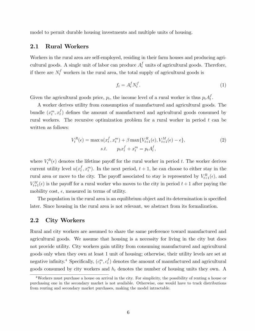
2.2 City Workers

Rural and city workers are assumed to share the same preference toward manufactured and

agricultural goods. We assume that housing is a necessity for living in the city but does

not provide utility. City workers gain utility from consuming manufactured and agricultural

goods only when they own at least 1 unit of housing; otherwise, their utility levels are set at

negative infinity.4 Specifically, (cmt , cft ) denotes the amount of manufactured and agricultural

goods consumed by city workers and ht denotes the number of housing units they own. A

4Workers must purchase a house on arrival in the city. For simplicity, the possibility of renting a house orpurchasing one in the secondary market is not available. Otherwise, one would have to track distributionsfrom renting and secondary market purchases, making the model intractable.

6

city worker’s instantaneous utility function takes the following form:

U(cmt , cft , ht) =

{u(cmt , c

ft ) if ht ≥ 1

−∞ otherwise,

where this utility function implies that each worker is satiated by owning 1 unit of housing

and does not benefit from owning more. In equilibrium, manufacturing workers demand 1

unit of housing.

The optimization problem for workers who have already purchased a house in τ < t is

V Ct (ε, bτ ) = maxU(cmt , c

ft , ht) + βmax{V C

t+1(ε, bτ ), VRt+1(ε)}, (3)

s.t. ptcft + cmt + bτr

∗ = wmt .

Workers who have been in the city for more than one period have two state variables: their

utility cost from migration, ε, and mortgage debt from purchasing a house at time τ , bτ .

Here, V Ct (ε, bτ ) represents the lifetime payoff for a worker with disutility level ε and mortgage

debt bτ . The worker derives current utility U(cmt , cft , ht) and discounts future payoffs at rate

β by choosing between staying in the city, V Ct+1(ε, bτ ), or returning to the rural area, V

Rt+1(ε).

The worker spends his wage income, wmt , on consumption of manufactured and agricultural

goods and mortgage debt repayment, bτr∗.

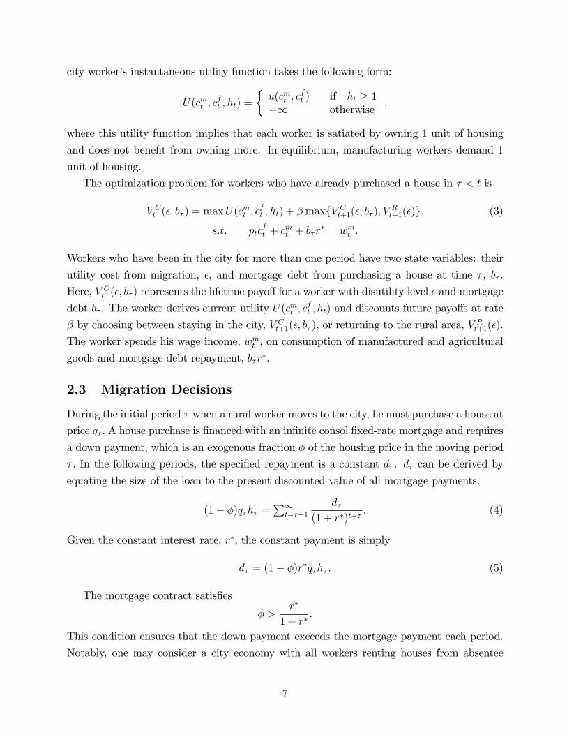
2.3 Migration Decisions

During the initial period τ when a rural worker moves to the city, he must purchase a house at

price qτ . A house purchase is financed with an infinite consol fixed-rate mortgage and requires

a down payment, which is an exogenous fraction φ of the housing price in the moving period

τ . In the following periods, the specified repayment is a constant dτ . dτ can be derived by

equating the size of the loan to the present discounted value of all mortgage payments:

(1− φ)qτhτ =∑∞

t=τ+1

dτ(1 + r∗)t−τ

. (4)

Given the constant interest rate, r∗, the constant payment is simply

dτ = (1− φ)r∗qτhτ . (5)

The mortgage contract satisfies

φ >r∗

1 + r∗.

This condition ensures that the down payment exceeds the mortgage payment each period.

Notably, one may consider a city economy with all workers renting houses from absentee

7

landlords who purchase them in advance to fill the demand. Maintaining the same housing

demand structure, one may then capture this pure rental case by setting φ = r∗/(1 + r∗),

under which an agent migrating in period τ signs a long-term rental agreement paying a rent

dτ every period based on the housing price.5 Thus, the pure rental market can be viewed as a

special case of our model (this case is discussed in more detail in Section 4.2). As elaborated

in Section 4, abstracting from the rental market in this model gives a conservative prediction

of the changes in housing and land prices.

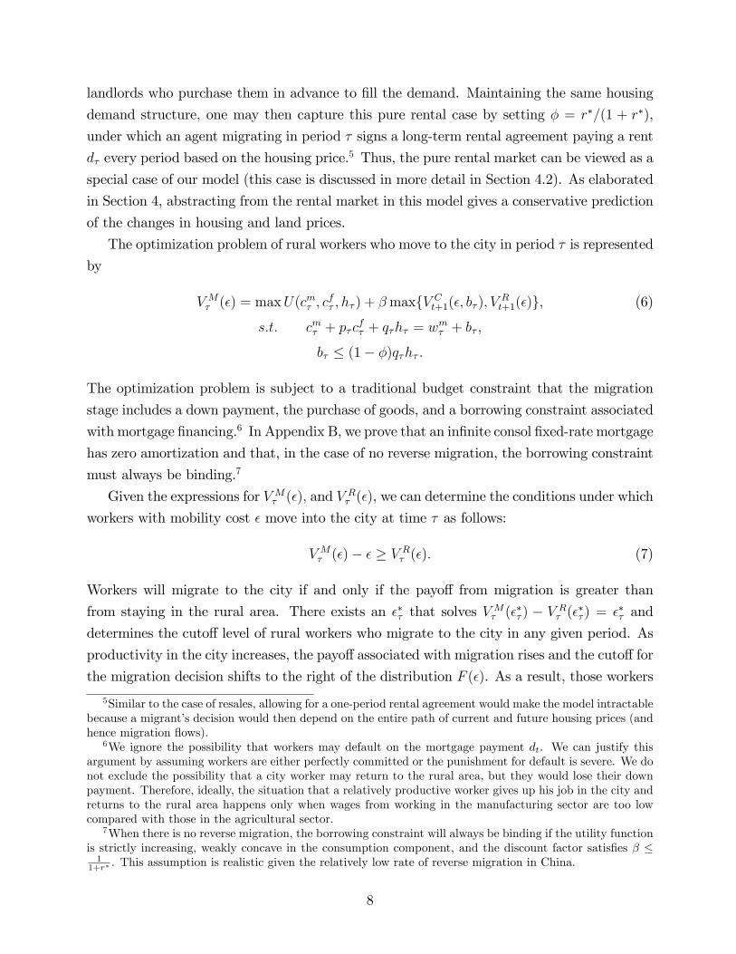
The optimization problem of rural workers who move to the city in period τ is represented

by

V Mτ (ε) = maxU(cmτ , c

fτ , hτ ) + βmax{V C

t+1(ε, bτ ), VRt+1(ε)}, (6)

s.t. cmτ + pτcfτ + qτhτ = wmτ + bτ ,

bτ ≤ (1− φ)qτhτ .

The optimization problem is subject to a traditional budget constraint that the migration

stage includes a down payment, the purchase of goods, and a borrowing constraint associated

with mortgage financing.6 In Appendix B, we prove that an infinite consol fixed-rate mortgage

has zero amortization and that, in the case of no reverse migration, the borrowing constraint

must always be binding.7

Given the expressions for V Mτ (ε), and V R

τ (ε), we can determine the conditions under which

workers with mobility cost ε move into the city at time τ as follows:

V Mτ (ε)− ε ≥ V R

τ (ε). (7)

Workers will migrate to the city if and only if the payoff from migration is greater than

from staying in the rural area. There exists an ε∗τ that solves VMτ (ε∗τ ) − V R

τ (ε∗τ ) = ε∗τ and

determines the cutoff level of rural workers who migrate to the city in any given period. As

productivity in the city increases, the payoffassociated with migration rises and the cutoff for

the migration decision shifts to the right of the distribution F (ε). As a result, those workers

5Similar to the case of resales, allowing for a one-period rental agreement would make the model intractablebecause a migrant’s decision would then depend on the entire path of current and future housing prices (andhence migration flows).

6We ignore the possibility that workers may default on the mortgage payment dt. We can justify thisargument by assuming workers are either perfectly committed or the punishment for default is severe. We donot exclude the possibility that a city worker may return to the rural area, but they would lose their downpayment. Therefore, ideally, the situation that a relatively productive worker gives up his job in the city andreturns to the rural area happens only when wages from working in the manufacturing sector are too lowcompared with those in the agricultural sector.

7When there is no reverse migration, the borrowing constraint will always be binding if the utility functionis strictly increasing, weakly concave in the consumption component, and the discount factor satisfies β ≤1

1+r∗ . This assumption is realistic given the relatively low rate of reverse migration in China.

8

initially unwilling to move now decide to migrate.

At the aggregate level, the incremental flow of migrants from the previous period is

represented by

∆F ∗τ (ε∗τ , ε∗τ−1) = F (ε∗τ )− F (ε∗τ−1). (8)

The flow of migrants is the key driver of housing and land prices in the model.

2.4 Manufacturing Sector

The manufactured goods market is perfectly competitive. For simplicity, labor is the only

productive input abstracting from capital. In the quantitative analysis, increases in the

capital-labor ratio would be included in productivity growth. The production technology of

the manufacturing sector is linear in labor:

Y mt = Amt N

mt , (9)

where Amt denotes the labor productivity in the manufacturing sector at period t. The em-

ployment level in the city is endogenous and depends on the disutility cutoff for migration

decisions, Nmt = F (ε∗t ). The price of manufactured goods is normalized to 1, and the opti-

mality conditions imply

wmt = Amt . (10)

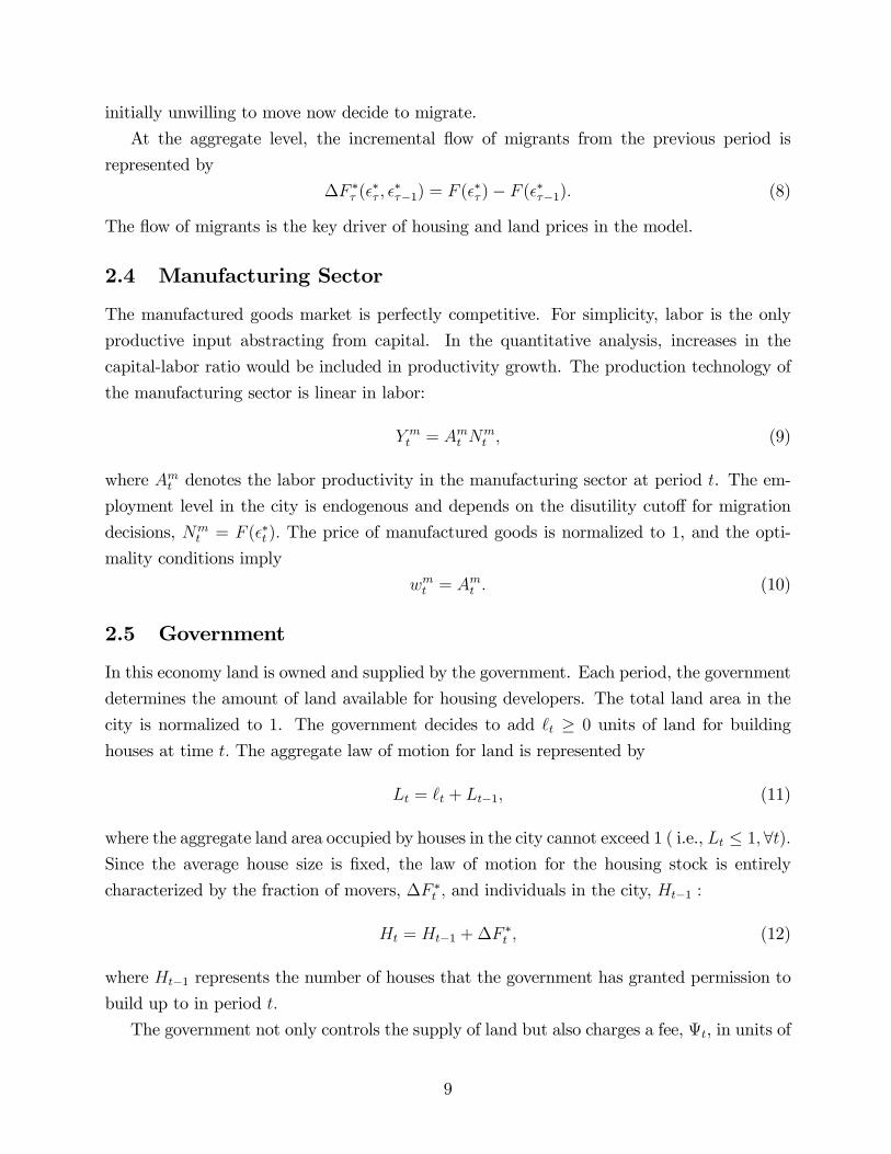
2.5 Government

In this economy land is owned and supplied by the government. Each period, the government

determines the amount of land available for housing developers. The total land area in the

city is normalized to 1. The government decides to add `t ≥ 0 units of land for building

houses at time t. The aggregate law of motion for land is represented by

Lt = `t + Lt−1, (11)

where the aggregate land area occupied by houses in the city cannot exceed 1 ( i.e., Lt ≤ 1,∀t).Since the average house size is fixed, the law of motion for the housing stock is entirely

characterized by the fraction of movers, ∆F ∗t , and individuals in the city, Ht−1 :

Ht = Ht−1 + ∆F ∗t , (12)

where Ht−1 represents the number of houses that the government has granted permission to

build up to in period t.

The government not only controls the supply of land but also charges a fee, Ψt, in units of

9

manufactured goods, to housing developers, which determines the number of permits granted:

Ψt = ψHt−1, (13)

where the average land leasing fee, ψ > 0, is constant over time. A larger number of permits

granted in the past, Ht−1, implies a higher fixed construction fee. This assumption captures

public concern about congestion and overcrowding in cities.

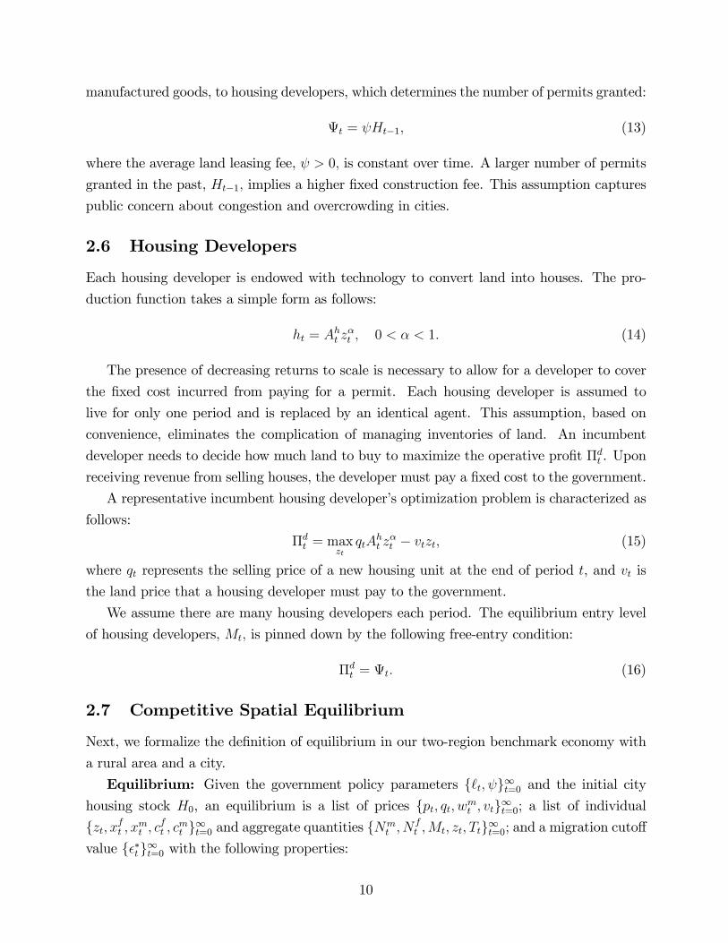
2.6 Housing Developers

Each housing developer is endowed with technology to convert land into houses. The pro-

duction function takes a simple form as follows:

ht = Aht zαt , 0 < α < 1. (14)

The presence of decreasing returns to scale is necessary to allow for a developer to cover

the fixed cost incurred from paying for a permit. Each housing developer is assumed to

live for only one period and is replaced by an identical agent. This assumption, based on

convenience, eliminates the complication of managing inventories of land. An incumbent

developer needs to decide how much land to buy to maximize the operative profit Πdt . Upon

receiving revenue from selling houses, the developer must pay a fixed cost to the government.

A representative incumbent housing developer’s optimization problem is characterized as

follows:

Πdt = max

ztqtA

ht z

αt − vtzt, (15)

where qt represents the selling price of a new housing unit at the end of period t, and vt is

the land price that a housing developer must pay to the government.

We assume there are many housing developers each period. The equilibrium entry level

of housing developers, Mt, is pinned down by the following free-entry condition:

Πdt = Ψt. (16)

2.7 Competitive Spatial Equilibrium

Next, we formalize the definition of equilibrium in our two-region benchmark economy with

a rural area and a city.

Equilibrium: Given the government policy parameters {`t, ψ}∞t=0 and the initial cityhousing stock H0, an equilibrium is a list of prices {pt, qt, wmt , vt}∞t=0; a list of individual{zt, xft , xmt , c

ft , c

mt }∞t=0 and aggregate quantities {Nm

t , Nft ,Mt, zt, Tt}∞t=0; and a migration cutoff

value {ε∗t}∞t=0 with the following properties:

10

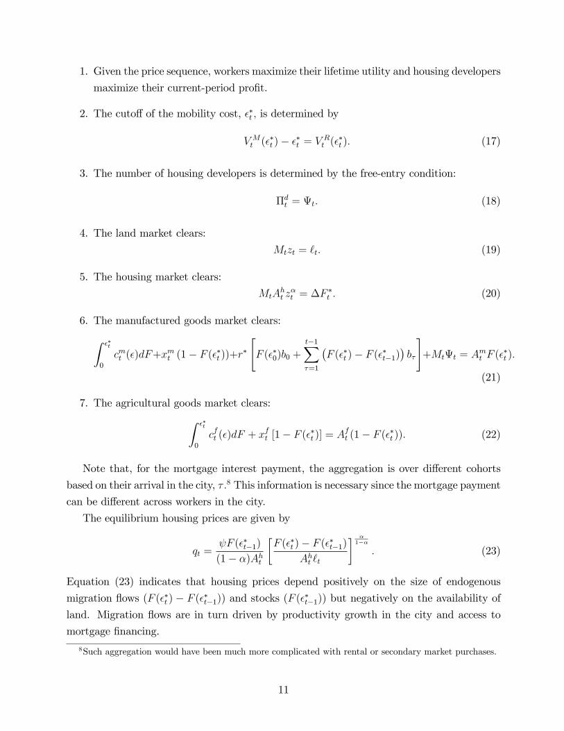
1. Given the price sequence, workers maximize their lifetime utility and housing developers

maximize their current-period profit.

2. The cutoff of the mobility cost, ε∗t , is determined by

V Mt (ε∗t )− ε∗t = V R

t (ε∗t ). (17)

3. The number of housing developers is determined by the free-entry condition:

Πdt = Ψt. (18)

4. The land market clears:

Mtzt = `t. (19)

5. The housing market clears:

MtAht z

αt = ∆F ∗t . (20)

6. The manufactured goods market clears:∫ ε∗t

0

cmt (ε)dF+xmt (1− F (ε∗t ))+r∗

[F (ε∗0)b0 +

t−1∑τ=1

(F (ε∗t )− F (ε∗t−1)

)bτ

]+MtΨt = Amt F (ε∗t ).

(21)

7. The agricultural goods market clears:∫ ε∗t

0

cft (ε)dF + xft [1− F (ε∗t )] = Aft (1− F (ε∗t )). (22)

Note that, for the mortgage interest payment, the aggregation is over different cohorts

based on their arrival in the city, τ .8 This information is necessary since the mortgage payment

can be different across workers in the city.

The equilibrium housing prices are given by

qt =ψF (ε∗t−1)

(1− α)Aht

[F (ε∗t )− F (ε∗t−1)

Aht `t

] α1−α

. (23)

Equation (23) indicates that housing prices depend positively on the size of endogenous

migration flows (F (ε∗t ) − F (ε∗t−1)) and stocks (F (ε∗t−1)) but negatively on the availability of

land. Migration flows are in turn driven by productivity growth in the city and access to

mortgage financing.

8Such aggregation would have been much more complicated with rental or secondary market purchases.

11

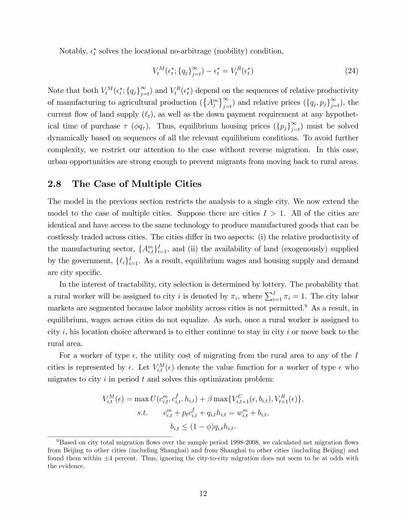
Notably, ε∗t solves the locational no-arbitrage (mobility) condition,

V Mt (ε∗t ; {qj}

∞j=t)− ε

∗t = V R

t (ε∗t ) (24)

Note that both V Mt (ε∗t ; {qj}

∞j=t) and V

Rt (ε∗t ) depend on the sequences of relative productivity

of manufacturing to agricultural production ({Amj}∞j=t) and relative prices ({qj, pj}∞j=t), the

current flow of land supply (`t), as well as the down payment requirement at any hypothet-

ical time of purchase τ (φqτ ). Thus, equilibrium housing prices ({pj}∞j=t) must be solveddynamically based on sequences of all the relevant equilibrium conditions. To avoid further

complexity, we restrict our attention to the case without reverse migration. In this case,

urban opportunities are strong enough to prevent migrants from moving back to rural areas.

2.8 The Case of Multiple Cities

The model in the previous section restricts the analysis to a single city. We now extend the

model to the case of multiple cities. Suppose there are cities I > 1. All of the cities are

identical and have access to the same technology to produce manufactured goods that can be

costlessly traded across cities. The cities differ in two aspects: (i) the relative productivity of

the manufacturing sector, {Ami,t}Ii=1, and (ii) the availability of land (exogenously) suppliedby the government, {`i}Ii=1. As a result, equilibrium wages and housing supply and demand

are city specific.

In the interest of tractability, city selection is determined by lottery. The probability that

a rural worker will be assigned to city i is denoted by πi, where∑I

i=1 πi = 1. The city labor

markets are segmented because labor mobility across cities is not permitted.9 As a result, in

equilibrium, wages across cities do not equalize. As such, once a rural worker is assigned to

city i, his location choice afterward is to either continue to stay in city i or move back to the

rural area.

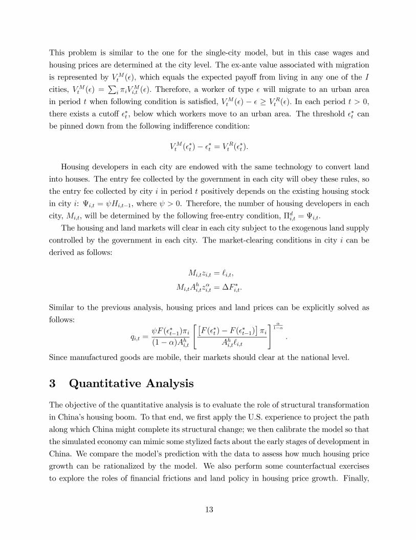
For a worker of type ε, the utility cost of migrating from the rural area to any of the I

cities is represented by ε. Let V Mi,t (ε) denote the value function for a worker of type ε who

migrates to city i in period t and solves this optimization problem:

V Mi,t (ε) = maxU(cmi,t, c

fi,t, hi,t) + βmax{V C

i,t+1(ε, bi,t), VRt+1(ε)},

s.t. cmi,t + ptcfi,t + qi,thi,t = wmi,t + bi,t,

bi,t ≤ (1− φ)qi,thi,t.

9Based on city total migration flows over the sample period 1998-2008, we calculated net migration flowsfrom Beijing to other cities (including Shanghai) and from Shanghai to other cities (including Beijing) andfound them within ±4 percent. Thus, ignoring the city-to-city migration does not seem to be at odds withthe evidence.

12

This problem is similar to the one for the single-city model, but in this case wages and

housing prices are determined at the city level. The ex-ante value associated with migration

is represented by V Mt (ε), which equals the expected payoff from living in any one of the I

cities, V Mt (ε) =

∑i πiV

Mi,t (ε). Therefore, a worker of type ε will migrate to an urban area

in period t when following condition is satisfied, V Mt (ε) − ε ≥ V R

t (ε). In each period t > 0,

there exists a cutoff ε∗t , below which workers move to an urban area. The threshold ε∗t can

be pinned down from the following indifference condition:

V Mt (ε∗t )− ε∗t = V R

t (ε∗t ).

Housing developers in each city are endowed with the same technology to convert land

into houses. The entry fee collected by the government in each city will obey these rules, so

the entry fee collected by city i in period t positively depends on the existing housing stock

in city i: Ψi,t = ψHi,t−1, where ψ > 0. Therefore, the number of housing developers in each

city, Mi,t, will be determined by the following free-entry condition, Πdi,t = Ψi,t.

The housing and land markets will clear in each city subject to the exogenous land supply

controlled by the government in each city. The market-clearing conditions in city i can be

derived as follows:

Mi,tzi,t = `i,t,

Mi,tAhi,tz

αi,t = ∆F ∗i,t.

Similar to the previous analysis, housing prices and land prices can be explicitly solved as

follows:

qi,t =ψF (ε∗t−1)πi

(1− α)Ahi,t

[[F (ε∗t )− F (ε∗t−1)

]πi

Ahi,t`i,t

] α1−α

.

Since manufactured goods are mobile, their markets should clear at the national level.

3 Quantitative Analysis

The objective of the quantitative analysis is to evaluate the role of structural transformation

in China’s housing boom. To that end, we first apply the U.S. experience to project the path

along which China might complete its structural change; we then calibrate the model so that

the simulated economy can mimic some stylized facts about the early stages of development in

China. We compare the model’s prediction with the data to assess how much housing price

growth can be rationalized by the model. We also perform some counterfactual exercises

to explore the roles of financial frictions and land policy in housing price growth. Finally,

13

we extend the quantitative analysis to the multiple city case, which allows us to evaluate

for various cities the different contributions structural change might make to housing price

growth.

3.1 Projection of the Chinese Population and Land Distribution

In 1840 almost 90 percent of the total U.S. population lived in rural areas. This percentage

steadily declined to about 3 percent in 1990 and has since remained at about 3 percent.

Because the fraction of the population living in rural areas is a main indicator of the progress

of structural transformation, the United States is viewed as having completed its structural

transformation by 1990. In 2012, the agricultural share of employment in China is still over

30 percent and the fraction of urban employment is around 50 percent as can be seen in

Figure 3.10

Calculating the path of future prices requires making different assumptions about the

length of the structural transformation process. In the baseline case, we assume that the

path of China’s structural transformation will take another 50 years. Under this assumption,

in the year 2065 urban employment in China will become steady thereafter. Our algorithm

is simply as follows: We assume net migration flow into urban area will continue to grow

until the year 2020, and then, it will steadily decline as shown in the top left panel of Figure

4. The definition of net migration flows from rural to urban areas include permanent and

temporary permits where many of the latter, mostly renting, but are later granted permanent

permits. Overall, the time path for the fraction of urban employment is plotted in the top

right panel of Figure 4. By 2065, the fraction of urban employment will reach 95 percent.11

We also perform a similar projection algorithm for the residential land supply. We back

out the annual residential land supply from the data by using “land space purchased this

year by real-estate enterprises” divided by “total land area for inhabitation, mining, and

manufacturing”, where we assume that the fraction of land for residential use is constant

over time. Based on currently available data for China, we extrapolate the residential land

supply series to 2065. The stock and the flow are summarized in the bottom panels of Figure

4.12

10While there is discrepancy in the definition of urban areas between these two large economies, the contrastis sharp regardless.11Note that there may be more optimistic projections on the progress of structural transformation in China,

with a much faster transition for China than the United States. The conjecture above is provided as a startingpoint. As a robustness check, we performed various exercises with more optimistic and pessimistic projectedpaths. While the results have some effects in the very long-run, but they have only a minor impact on thesimulated dynamics of housing prices between 1998 and 2012.12The results for the period 1998-2012 do not appear to be extremely sensitive to slightly different paths

of the residential land supply.

14

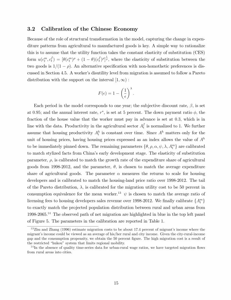
3.2 Calibration of the Chinese Economy

Because of the role of structural transformation in the model, capturing the change in expen-

diture patterns from agricultural to manufactured goods is key. A simple way to rationalize

this is to assume that the utility function takes the constant elasticity of substitution (CES)

form u(cmt , cft ) = [θ(cmt )ρ + (1 − θ)(cft )

ρ]1ρ , where the elasticity of substitution between the

two goods is 1/(1 − ρ). An alternative specification with non-homothetic preferences is dis-

cussed in Section 4.5. A worker’s disutility level from migration is assumed to follow a Pareto

distribution with the support on the interval [1,∞) :

F (ε) = 1−(

1

ε

)λ.

Each period in the model corresponds to one year; the subjective discount rate, β, is set

at 0.95; and the annual interest rate, r∗, is set at 5 percent. The down payment ratio φ, the

fraction of the house value that the worker must pay in advance is set at 0.3, which is in

line with the data. Productivity in the agricultural sector Aft is normalized to 1. We further

assume that housing productivity Aht is constant over time. Since Ah matters only for the

unit of housing prices, having housing prices expressed as an index allows the value of Ah

to be immediately pinned down. The remaining parameters {θ, ρ, α, ψ, λ, Amt } are calibratedto match stylized facts from China’s early development stage. The elasticity of substitution

parameter, ρ, is calibrated to match the growth rate of the expenditure share of agricultural

goods from 1998-2012, and the parameter, θ, is chosen to match the average expenditure

share of agricultural goods. The parameter α measures the returns to scale for housing

developers and is calibrated to match the housing-land price ratio over 1998-2012. The tail

of the Pareto distribution, λ, is calibrated for the migration utility cost to be 50 percent in

consumption equivalence for the mean worker.13 ψ is chosen to match the average ratio of

licensing fees to housing developers sales revenue over 1998-2012. We finally calibrate {Amt }to exactly match the projected population distribution between rural and urban areas from

1998-2065.14 The observed path of net migration are highlighted in blue in the top left panel

of Figure 5. The parameters in the calibration are reported in Table 1.

13Zhu and Zhang (1996) estimate migration costs to be about 17.4 percent of migrant’s income where themigrant’s income could be viewed as an average of his/her rural and city income. Given the city-rural-incomegap and the consumption propensity, we obtain the 50 percent figure. The high migration cost is a result ofthe restricted “hukou”system that limits regional mobility.14In the absence of quality time-series data for urban-rural wage ratios, we have targeted migration flows

from rural areas into cities.

15

3.3 Quantitative Results: National Benchmark

The main quantitative analysis focuses on the model’s ability to generate movements in

housing. The model generates yearly predictions for the variables that can then be compared

with the data. The evaluation of the model’s performance is based on average growth rates

for the period 1998-2012. The results are summarized in Table 2 (top panel).

In China, the average housing price growth rate is 9.7 percent and the model predicts

6.4 percent in the overall sample. Nevertheless, the performance improves by measuring the

model’s generated data in a restricted subsample for the period 2003-2007. The model is

able to generate a housing price growth rate of 6.6 percent while the data counterpart is 9.1

percent. This finding suggests that in the aftermath of the financial crisis, the contribution

of migration to house prices has weakened relative to other factors.

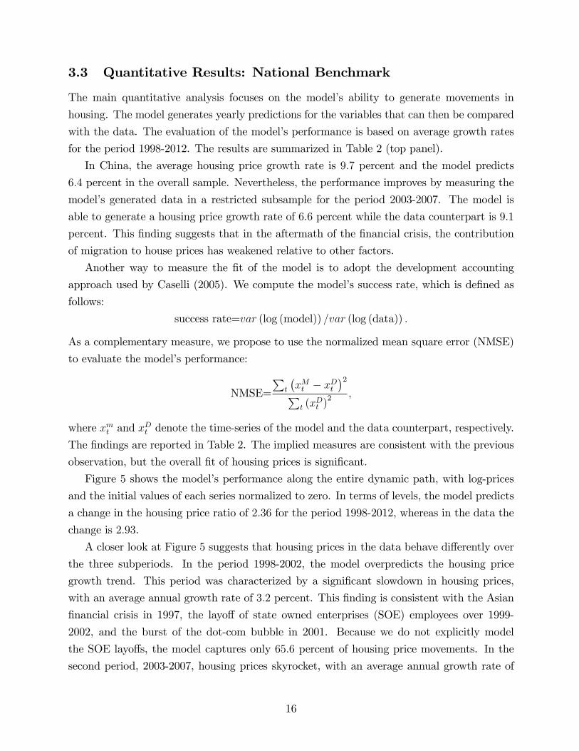
Another way to measure the fit of the model is to adopt the development accounting

approach used by Caselli (2005). We compute the model’s success rate, which is defined as

follows:

success rate=var (log (model)) /var (log (data)) .

As a complementary measure, we propose to use the normalized mean square error (NMSE)

to evaluate the model’s performance:

NMSE=

∑t

(xMt − xDt

)2∑t (xDt )

2 ,

where xmt and xDt denote the time-series of the model and the data counterpart, respectively.

The findings are reported in Table 2. The implied measures are consistent with the previous

observation, but the overall fit of housing prices is significant.

Figure 5 shows the model’s performance along the entire dynamic path, with log-prices

and the initial values of each series normalized to zero. In terms of levels, the model predicts

a change in the housing price ratio of 2.36 for the period 1998-2012, whereas in the data the

change is 2.93.

A closer look at Figure 5 suggests that housing prices in the data behave differently over

the three subperiods. In the period 1998-2002, the model overpredicts the housing price

growth trend. This period was characterized by a significant slowdown in housing prices,

with an average annual growth rate of 3.2 percent. This finding is consistent with the Asian

financial crisis in 1997, the layoff of state owned enterprises (SOE) employees over 1999-

2002, and the burst of the dot-com bubble in 2001. Because we do not explicitly model

the SOE layoffs, the model captures only 65.6 percent of housing price movements. In the

second period, 2003-2007, housing prices skyrocket, with an average annual growth rate of

16

15.1 percent. This finding is consistent with fast economic growth and further deregulation

of the migration policy and the financial sector in conjunction with the government’s reduced

control of urban land and housing permits. For this subperiod, the model captures housing

price movements from 2004 forward and explains only 65.1 percent of this movement because

of underprediction carried from the previous subperiod.

Remark: It is informative to consider the case of a pure rental market, re-calibrating themodel by setting φ = r∗/(1 + r∗) = 4.76%. In this case, the new migrants are indifferent

between owning or renting. With no down payment requirement, it is easier for rural workers

to migrate to the city. Our quantitative results suggest that the effects from this increased

migration flow dominate the general equilibrium effects, which results in the model predicting

higher housing prices. In this case, the model accounts for 87.0 percent of the movement in

housing prices. With tenant choices, the model’s predictive power would be somewhere

between the benchmark case and the pure rental case. Thus, one may conclude that our

benchmark model provides a conservative prediction of the changes in housing.

The model can be used to understand the relative importance of the different driving

forces of housing prices over the sample period 1998-2012. To do this, we decompose the

contributions of the various factors (the down payment constraint, entry fee, land supply

policy, and productivity of the manufacturing sector) relative to the benchmark model. This

decomposition maintains the calibrated parameters of the benchmark values and changes one

factor at a time. More specifically, the decomposition considers the following counterfactuals

for each factor:

• Entry fee: The magnitude of the entry fee paid by land developers depends positivelyon the current city population. A higher value of ψ implies a higher entry fee and

fewer developers. The benchmark value in the calibration is 4.5. In the counterfactual

analysis, the value of ψt varies each period so that government revenue remains constant

at its level in the initial period t = 0. When the population of the city grows, the

computed value of ψt decreases over time, inducing the entry of housing developers

and increasing housing production. In equilibrium, more houses lead to lower housing

prices and a higher level of migrants. By comparing the counterfactual price with the

benchmark price, it is possible to compute the relative contribution of the entry fee.

• Land supply: In the counterfactual experiment, the flow of land supplied by the

government to the market is fixed at the initial high level, `t = `0, for all t. The relative

increase in the land supply generates an upward shift in the housing supply, leading to

a decrease in housing prices and an increase in the number of migrants.

17

• Mortgage financing (down payment constraint): The counterfactual considersno mortgage financing, φ = 1, instead of the benchmark value of 0.3. The elimination

of mortgage financing should drive down housing demand and, hence, housing prices.

• Productivity: Productivity acts as the residual in the decomposition exercise. Thatis, within our framework, in the absence of other variations beyond the above-mentioned

factors, productivity growth explains the remaining portions of the increases in housing

prices and the average fraction of migrants in the city population.

The results of the decomposition are summarized in Table 2 (bottom panel), which shows

by time period the percentage increases in housing prices due to each single factor. For

example, in the case of land supply controls, the decomposition compares the benchmark

with an economy that has the same increased availability of land as in the initial years

(1998-2002). The increased availability of land leads to a decrease in housing prices and an

increase in the migrant population in the city. The data for the period 1998-2012 reveal

the following: Tightening the land supply policy in the benchmark case contributes to 36.0

percent of housing price growth. The decomposition results suggest that supply factors are

the most important factor for increases in housing prices, accounting for 62.7 percent of

the total change in the model, whereas productivity (income) accounts for only about 20

percent. The role of productivity becomes more important over time while the contribution

of supply factors diminishes. This would be consistent with the rising role of an effective

“world factory”that China played during its urbanization process. Over the entire sample

period, the contributions of access to credit to all indicators are below 20 percent.

3.4 Quantitative Results: Multiple-City Model

One may question whether structural transformation can still explain the rapid growth of

housing prices in large cities. This section explores the contribution of urbanization to the

dynamics of housing and land prices at the city level. Although the size of migration flows

could be responsible for the rapid increase in housing prices in many cities in China, other fac-

tors (i.e., different housing supply restrictions and land regulations) could also be important.

For better illustration, the analysis is restricted to the two largest cities in China: Beijing

and Shanghai. These two cities accounted for 6.5 percent of the entire urban population in

2011.

As shown in Figure 6, the rapid population growth naturally led to housing booms in these

two major cities with housing prices growing above the national average. Housing prices in

Beijing remained relatively stable until 2005; in contrast, housing prices in Shanghai grew

continuously, with a more rapid trend starting in 2004.

18

The multiple-city model has to be consistent not only with the rural-urban migration but

also with the change in city population. The quantitative analysis maintains the values of

the preference and technology parameters of the single-city model with these exceptions: the

exogenous probability of migrating to city i from the rural area, πi; the relative manufacturing

productivity in city i, {Ai,t}; and the total residential land area in city i, {Li,t}. When thereare I > 1 cities in the urban area, the share of the population in city i, ni,t, is denoted as

follows, where Ni,t denotes the total population in city i and NRt denotes the total population

in the rural area:

ni,t =Ni,t∑I

i=1Ni,t +NRt

.

When the total population is normalized to 1, the growth rate of ni,t can be shown to be

equivalent to the growth rate of Ni,t:

4Ni,t

Ni,t

=4ni,tni,t

.

Since each period a fraction πi of migrants moves to city i, it is implied that4Ni,t = −πiNRt .

Therefore, the growth rate of ni,t can be represented as follows:

4ni,tni,t

=4Ni,t

Ni,t

= −πi4NR

t

NRt

NRt

Ni,t

. (25)

The rule for assigning migrants to a particular city πi can be estimated from the equation

above. The change in the fraction of migrants in the populations of Beijing and Shanghai

between 1994 and 2011 was 52.75 percent and 45.65 percent, respectively.15 Therefore, using

equation (25), for that period the fractions of migrants flowing to Beijing and Shanghai are

3.4 and 3.9 percent, respectively.

In 1994, 1.03 percent and 1.17 percent of the total population of China lived in Beijing

and Shanghai, respectively; 26.8 percent lived in other cities, and 71.0 percent lived in rural

areas. Given the values of {nB,0, nS,0,πB, πs}, it is straightforward to calculate the sequencesof {nB,t} and {nS,t} from ni,t+1 = ni,t + πi(n

Rt − nRt+1), i ∈ {B, S,O}.

To complete the calibration of the multiple-city model it is necessary to determine the

land supply and the entry fee in each city. The total land area is 164, 100 square kilometers

in Beijing and 82, 400 in Shanghai. The annual residential land supply in each city from data

is still defined by using “land space purchased this year by real-estate enterprises”divided by

“total land area for inhabitation, mining and manufacturing,”where we have assumed that

the fraction of land for residential use is constant over time in each city. The data for the

15We use a longer span of data to capture the long-run trend and mitigate large fluctuations in migrationflows from events such as the SOE layoffs and the SARS epidemic (discussed below).

19

residential land supply in each city are plotted in Figure 6. Consistent with the aggregate

model, in each city an entry fee is collected by the local government.

The migration flow is combined with supply factors to generate a sequence of housing

and land prices for each city for the period 1998-2012. As shown in Table 3 (top panel), the

average housing price growth rate in the data is 4.5 and 12.4 percent in Beijing and Shanghai

from 1998 to 2012, respectively, while our model predicts 8.1 percent for each city. If we

restrict the analysis to the period 1998-2007, our model performs better only in predicting

housing price growth in Shanghai. As for the success rate, the model seems to be successful

in predicting housing price growth in both cities. The NMSE remains low for housing prices

in both cities. The dynamic evolution of model-predicted housing prices over 1998-2012 with

the data is summarized in Figure 7. The model captures not only an important fraction

of the level change, but also the dynamic adjustment of house prices. To understand the

differential patterns across these two cities it is useful to decompose the sample into three

subperiods:

• 1998-2002: During this period the economy was affected by the financial crises inAsia and the burst of the dot-com bubble. During these years, China had high levels

of unemployment, especially for SOE workers. The gradual but deepening economic

reform encouraged more and more private enterprises to enter the market. Beijing, the

capital of China, was the headquarters for many SOE; thus, more workers were laid off

in Beijing than in Shanghai.

• 2003-2007: The spread of the SARS virus affected Beijing more severely in 2002 thanit did Shanghai in 2003 and reduced migration to Beijing. After 2003, the period

was characterized by rapid growth leading up to the 2008 Summer Olympic Games in

Beijing.

• 2008-2012: This is the burst of global financial crisis period.

The model captures a “flying geese” pattern of city development. As an early starter,

Beijing has transferred more and more industrial production to Shanghai and, hence, the

latter has attracted a larger labor force. This fact explains why housing prices in Shanghai

grew faster than in Beijing. Across the two cities and the three subperiods, the model

performs quite well except for Beijing in the second subperiod. As mentioned, the spread of

the SARS virus significantly reduced migration to Beijing. Since housing prices in the model

are critically driven by migration, the model predicts a much larger decline in housing prices

than found in the data. This underprediction is also responsible for the relatively low average

growth rate of housing prices.

20

Historically, Beijing and Shanghai have been the main industrialized cities in China. Ever

since the implementation of reform and open policy in China, these cities have received the

most rural migrants. The fact that the model can explain a sizable fraction of housing price

growth in both cities affi rms the idea that structural change plays a crucial role in housing

price growth in industrialized cities.

In the model, both cities have similar migration flows. The main differences in price

dynamics have to be the result of institutional differences operating through the supply

factors. To assess the relative importance of all factors, but in particular on the supply side,

we decompose the relative contribution of each factor for the full sample by subperiods, as

shown in Table 3 (bottom panel).

For both cities, supply factors are the most important driver of the increase in housing

prices, accounting for an average of 60.2 percent in Beijing and 53.2 percent in Shanghai.

These numbers are slightly lower than that for the nation reported in the single-city model.

The contribution of productivity in Beijing is similar to that at the national level, whereas

productivity plays a noticeably more important role in Shanghai, indicating that the ag-

glomerations could be critical in the largest city of China. We also find that productivity

becomes more important over time for explaining housing price movements during the last

subperiod. In the initial subperiod, the relatively higher income growth in Shanghai drives

the variation in housing prices across the two cities. The relatively low productivity in Bei-

jing captures the low growth in employment and migration due to the layoff of SOE workers.

Even though the relative contribution of productivity in the two cities is comparable in the

first and second subperiod, it is important to note the stagnation of housing prices in Beijing

due to a productivity slowdown. Again, the impact of the SARS virus is captured by low

migration flows and, hence, low income growth (productivity). Land supply becomes more

important in explaining Beijing’s housing prices during 2008-2012. The regulation of housing

developments through fees and land supply also plays an important role.

The quantitative findings indicate that the process of structural transformation can be

an important driver of housing prices, not only at the national level but also for large cities

such as Beijing and Shanghai, where housing booms have been particularly noticeable.

4 Extensions

This section extends the baseline model along several dimensions. The objective is to assess

the robustness of the main findings obtained in the benchmark model. The first modification

smooths the volatile migration flows. The next extension departs from direct ownership of

housing and considers the case where migrants rent houses perpetually. We then introduce

21

housing quality into our model in a parsimonious manner, to examine the potential role of

home upgrading in China’s housing boom. Moreover, we consider savings, the consumption

valuation of housing and the investment value of housing, to check the extent to which the

predictability of house price in China could be enhanced. Finally, we show that our model

with standard non-homothetic preferences is isomorphic to one with CES preferences.

4.1 Migration Flow Smoothing

In the baseline model, the annual flow of migrant workers is targeted for calibrating the rela-

tive productivity growth between the manufacturing and agricultural sectors. The volatility

of migration flows could imply unnecessary choppiness in productivity measures. It is there-

fore natural to consider a 5-year moving average of the series. In doing so, we can also

indirectly capture possible effects from delayed housing purchases present in the data. As

can be seen in Figure 8 (top left), the results are essentially unchanged relative to the baseline

model.

4.2 Pure Housing Rental

The baseline model assumes 100 percent homeownership in the urban areas. While the

homeownership rate is very high in China (over 80 percent), it is clear that some migrant

workers might not be able to afford to purchase a house immediately after their arrival in

the city. To assess the importance of this assumption, this section explores another extreme:

assuming that all migrants rent houses perpetually.

The case of tenant-occupied residency is captured by setting φ = r∗/(1 + r∗), where an

agent migrating in period τ signs a long-term rental agreement paying each period a fixed

rent dτ based on the housing price when the tenant moved in. Figure 8 (top right) shows

some noticeable improvements over the benchmark case. The prediction of housing price

growth under the pure rental case improves from 66 percent to 78 percent. This is because

renting mitigates the financial barriers to migration, thus leading to the prediction of higher

growth rates of housing. The differences between these two extreme cases can be indirectly

interpreted as the contribution of homeownership to housing prices.

4.3 Housing Quality

The benchmark model assumes that housing is a necessity to live in the urban area with-

out adding valuation to households. This section considers a simple departure that allows

for variations of housing quality entering a city worker’s utility function in a parsimonious

22

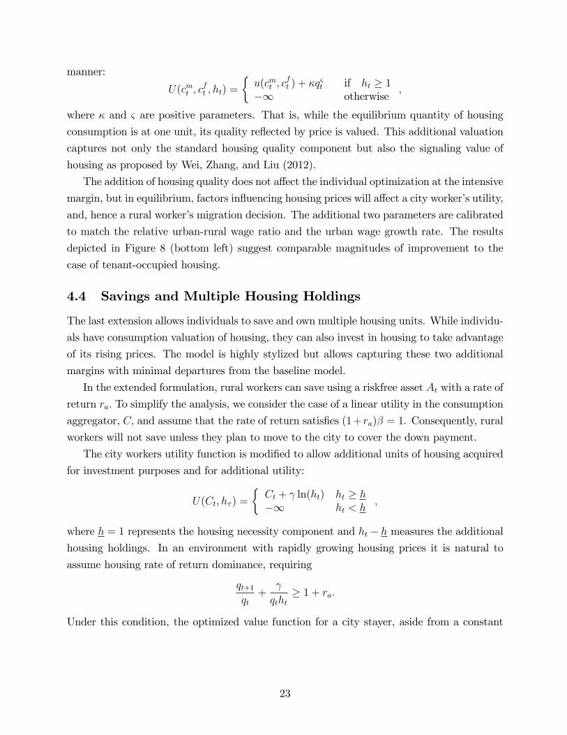
manner:

U(cmt , cft , ht) =

{u(cmt , c

ft ) + κqςt if ht ≥ 1

−∞ otherwise,

where κ and ς are positive parameters. That is, while the equilibrium quantity of housing

consumption is at one unit, its quality reflected by price is valued. This additional valuation

captures not only the standard housing quality component but also the signaling value of

housing as proposed by Wei, Zhang, and Liu (2012).

The addition of housing quality does not affect the individual optimization at the intensive

margin, but in equilibrium, factors influencing housing prices will affect a city worker’s utility,

and, hence a rural worker’s migration decision. The additional two parameters are calibrated

to match the relative urban-rural wage ratio and the urban wage growth rate. The results

depicted in Figure 8 (bottom left) suggest comparable magnitudes of improvement to the

case of tenant-occupied housing.

4.4 Savings and Multiple Housing Holdings

The last extension allows individuals to save and own multiple housing units. While individu-

als have consumption valuation of housing, they can also invest in housing to take advantage

of its rising prices. The model is highly stylized but allows capturing these two additional

margins with minimal departures from the baseline model.

In the extended formulation, rural workers can save using a riskfree asset At with a rate of

return ra. To simplify the analysis, we consider the case of a linear utility in the consumption

aggregator, C, and assume that the rate of return satisfies (1+ ra)β = 1. Consequently, rural

workers will not save unless they plan to move to the city to cover the down payment.

The city workers utility function is modified to allow additional units of housing acquired

for investment purposes and for additional utility:

U(Ct, hτ ) =

{Ct + γ ln(ht) ht ≥ h−∞ ht < h

,

where h = 1 represents the housing necessity component and ht − h measures the additionalhousing holdings. In an environment with rapidly growing housing prices it is natural to

assume housing rate of return dominance, requiring

qt+1qt

+γ

qtht≥ 1 + ra.

Under this condition, the optimized value function for a city stayer, aside from a constant

23

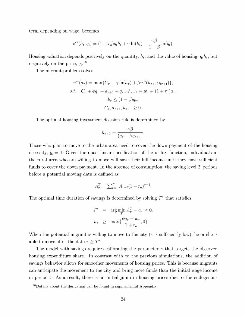
term depending on wage, becomes

vcs(ht; qt) = (1 + ra)qtht + γ ln(ht)−γβ

1− β ln(qt).

Housing valuation depends positively on the quantity, ht, and the value of housing, qtht, but

negatively on the price, qt.16

The migrant problem solves

vm(aτ ) = max{Cτ + γ ln(hτ ) + βvcs(hτ+1; qτ+1)},s.t. Cτ + φqτ + aτ+1 + qτ+1hτ+1 = wτ + (1 + ra)aτ ,

bτ ≤ (1− φ)qτ ,

Cτ , aτ+1, hτ+1 ≥ 0.

The optimal housing investment decision rule is determined by

hτ+1 =γβ

(qτ − βqτ+1).

Those who plan to move to the urban area need to cover the down payment of the housing

necessity, h = 1. Given the quasi-linear specification of the utility function, individuals in

the rural area who are willing to move will save their full income until they have suffi cient

funds to cover the down payment. In the absence of consumption, the saving level T periods

before a potential moving date is defined as

ATτ =∑T

t=1Aτ−t(1 + ra)τ−1.

The optimal time duration of savings is determined by solving T ∗ that satisfies

T ∗ = arg minTATτ − aτ ≥ 0.

aτ ≥ max{φqτ − wτ1 + ra

, 0}

When the potential migrant is willing to move to the city (ε is suffi ciently low), he or she is

able to move after the date τ ≥ T ∗.

The model with savings requires calibrating the parameter γ that targets the observed

housing expenditure share. In contrast with to the previous simulations, the addition of

savings behavior allows for smoother movements of housing prices. This is because migrants

can anticipate the movement to the city and bring more funds than the initial wage income

in period τ . As a result, there is an initial jump in housing prices due to the endogenous

16Details about the derivation can be found in supplemental Appendix.

24

decision of the moving date.

The quantitative findings associated with this extension are depicted in Figure 8 (bottom

right). This version of the model shows comparable magnitudes of improvement in housing

prices to the extension of tenant-occupied housing, suggesting that this extension is unlikely

to be critical for explaining the housing boom in China.

4.5 Non-Homothetic Preferences

In the standard structural transformation literature, it is common to consider non-homothetic

preferences to account for the transition from agriculture to manufacturing/services. For a

detailed review of the literature, see Herrendorf, Rogerson, and Valentinyi (2014). In this

subsection we show that our baseline specification with CES preferences is isomorphic to the

standard non-homothetic preferences as proposed by Kongsamut, Rebelo, and Xie (2001).

Recall individual preferences defined by a CES utility index U(xft , xmt ) = [θ(xft )

ρ + (1 −θ)(xmt )ρ]

1ρ and solving the optimized agricultural expenditure share, σft (pt), gives

σft (pt) =xftxt

=

(1 +

[(1− θ)θ

1

pρt

] 11−ρ)−1

.

Next, consider standard non-homothetic preferences in the Stone-Geary form, U(xft , xmt ) =

(xft −xf )η(xmt )1−η, with a minimum consumption requirement of agricultural goods, xf . This

preferences give an optimized agricultural expenditure share, σft (xt) :

σft (xt) = η + (1− η)xf

xt.

By the appropriate choice of xf , we show that the trend of the two expenditure shares is

the same. Given the baseline values of our preference specification θ = 0.50 and ρ = 0.80, we

calibrate the non-homothetic model to obtain η = 0.10 and xf = 0.50. Under the predicted

path of relative prices in the baseline model {pt}, the resulting expenditure shares in the twosetups are depicted in Figure 9 for the period 1998-2013. Consequently, the predictions on

housing and land price growth rates under the preference specifications are quantitatively

equivalent.

5 Conclusions

This paper uses a dynamic general equilibrium framework to investigate the role of structural

transformation in the rapid growth of housing prices in China. The benchmark economy

incorporates three major channels: (i) structural transformation, the increased productivity

25

of the manufacturing sector that leads to higher income and greater ability to pay; (ii) the

relatively inelastic supply of housing due to incremental city land released by the government

and the controlled entry of real estate developers through entry fees; and (iii) urbanization,

ongoing rural-urban migration that increases demand for urban housing. The quantitative

findings suggest that the process of structural transformation and the resulting urbanization

are important drivers of housing and land price movements in China. The model accounts for

80.5 percent of housing prices over 1998-2012 at the national level. The model performance

improves during the pre-financial tsunami period, accounting for 86.1 percent of housing over

1998-2012.

What important implications for policy are derived from this research? One is that

China’s housing prices are apparently driven primarily by structural transformation and the

induced migration from rural to urban areas. Thus, if China’s urban housing boom is a

concern, then our results suggest that to cool down the housing market, proper control of

supply factors such as land controls and developer entry regulations are likely to be much

more effective than mortgage restrictions.

In line with our model prediction, the tightened housing policy together with the growth

slowdown has led to a sluggish housing market in recent years. Events such as the turmoil

in the stock market combined with lower expectations about future growth are likely to

slow migrations flows from rural to urban areas. In the absence of supply changes, reduced

migration flows could have negative impacts on the housing market. Our approach is flexible

enough to be applied to different economic environments, and the implications of our analysis

have a larger scope than the Chinese experience. For example, in the case of U.S. urbanization

the pace of migration was relatively slow, which, combined with greater availability of land,

led to modest growth of housing prices during the whole process. On the contrary, countries

such as Japan, Korea, and Taiwan have experienced much faster migration flows and with

limited land availability, the urbanization process generated a noticeable housing boom.

References

[1] E. W. Bond, R. Riezman, and P. Wang (2014): “Trade, Urbanization and CapitalAccumulation in a Labor Surplus Economy,”Working Paper, Washington University inSt. Louis.

[2] K. Chen and Y. Wen (2014): “The Great Housing Bubble of China,”Mimeo.

[3] M. Davis and J. Heathcote (2005): “Housing and the Business Cycle,” InternationalEconomic Review, 46, 751—784.

26

[4] Y. Deng, J. Gyourko, and J. Wu (2015): “Evaluating the Risk of Chinese HousingMarkets: What We Know and What We Need to Know,”NBER, Cambridge, MA.

[5] H. Fang, Q. Gu, and L. Zhou (2014): “The Gradients of Power: Evidence from theChinese Housing Market,”National Bureau of Economic Research.

[6] C. Garriga, R. Manuelli, and A. Peralta-Alva. (2012): “A Model of Price Swings in theHousing Market,”Working Paper 2012-022, Federal Reserve Bank of St. Louis.

[7] G. Glomm, (1992): “A Model of Growth and Migration,”Canadian Journal of Eco-nomics, 25, 901-922.

[8] G.D. Hansen and E.C. Prescott. (2002): “Malthus to Solow,”American Economic Re-view, 92(4), 1205-1217.

[9] B. Herrendorf, R. Rogerson, and A. Valentinyi (2014): “Growth and Structural Trans-formation,”Handbook of Economic Growth, (2), 855—941.

[10] P. Kongsamut, S. Rebelo, and D. Xie. (2001): “Beyond Balanced Growth,”Review ofEconomic Studies, 68 (4): 869-882.

[11] P.J. Liao, Y.-C. Wang, P. Wang, and C.K. Yip (2014): “Education and Rural-urbanMigration: The Role of Zhaosheng in China,”Working Paper, Chinese University ofHong Kong.

[12] R. E. Lucas, Jr. (2004): “Life Earnings and Rural-Urban Migration,”Journal of PoliticalEconomy, 112, S29-S59.

[13] R. Ngai and C. Pissarides. (2007): “Structural Change in a Multi-Sector Model ofGrowth,”American Economic Review, 97, 429-443.

[14] S. Wei, X. Zhang, and Y. Liu. (2012): “Status Competition and Housing Prices,”Mimeo.

[15] X. Zhu. (2012): “Understanding China’s Growth: Past, Present, and Future,”Journalof Economic Perspectives 26 (4), 103-124.

[16] C. Zhu and Y. Zhang. (1996): “Cost and Benefit of Rural Children in the XianyangProvince of China,”Population and Economics, 5, 13-22.

27

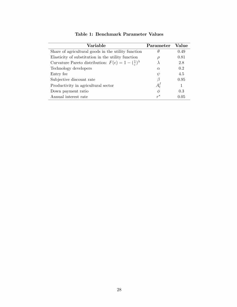
Table 1: Benchmark Parameter Values

Variable Parameter ValueShare of agricultural goods in the utility function θ 0.49Elasticity of substitution in the utility function ρ 0.81Curvature Pareto distribution: F (ε) = 1− (1

ε)λ λ 2.8

Technology developers α 0.2Entry fee ψ 4.5Subjective discount rate β 0.95Productivity in agricultural sector Aft 1Down payment ratio φ 0.3Annual interest rate r∗ 0.05

28

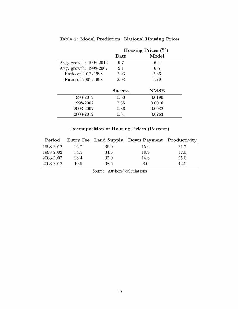
Table 2: Model Prediction: National Housing Prices

Housing Prices (%)Data Model

Avg. growth: 1998-2012 9.7 6.4Avg. growth: 1998-2007 9.1 6.6Ratio of 2012/1998 2.93 2.36Ratio of 2007/1998 2.08 1.79

Success NMSE1998-2012 0.60 0.01901998-2002 2.35 0.00162003-2007 0.36 0.00822008-2012 0.31 0.0263

Decomposition of Housing Prices (Percent)

Period Entry Fee Land Supply Down Payment Productivity1998-2012 26.7 36.0 15.6 21.71998-2002 34.5 34.6 18.9 12.02003-2007 28.4 32.0 14.6 25.02008-2012 10.9 38.6 8.0 42.5

Source: Authors’calculations

29

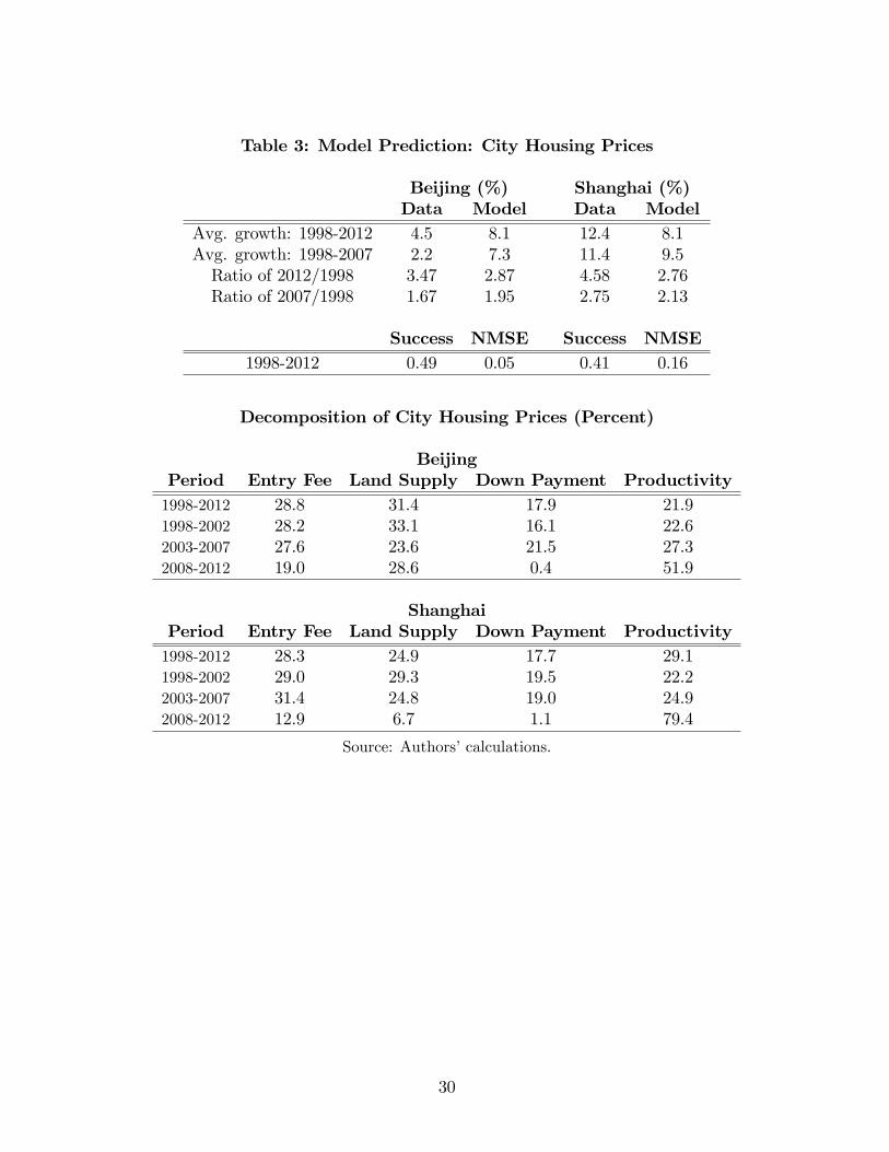
Table 3: Model Prediction: City Housing Prices

Beijing (%) Shanghai (%)Data Model Data Model

Avg. growth: 1998-2012 4.5 8.1 12.4 8.1Avg. growth: 1998-2007 2.2 7.3 11.4 9.5Ratio of 2012/1998 3.47 2.87 4.58 2.76Ratio of 2007/1998 1.67 1.95 2.75 2.13

Success NMSE Success NMSE1998-2012 0.49 0.05 0.41 0.16

Decomposition of City Housing Prices (Percent)

BeijingPeriod Entry Fee Land Supply Down Payment Productivity1998-2012 28.8 31.4 17.9 21.91998-2002 28.2 33.1 16.1 22.62003-2007 27.6 23.6 21.5 27.32008-2012 19.0 28.6 0.4 51.9

ShanghaiPeriod Entry Fee Land Supply Down Payment Productivity1998-2012 28.3 24.9 17.7 29.11998-2002 29.0 29.3 19.5 22.22003-2007 31.4 24.8 19.0 24.92008-2012 12.9 6.7 1.1 79.4

Source: Authors’calculations.

30

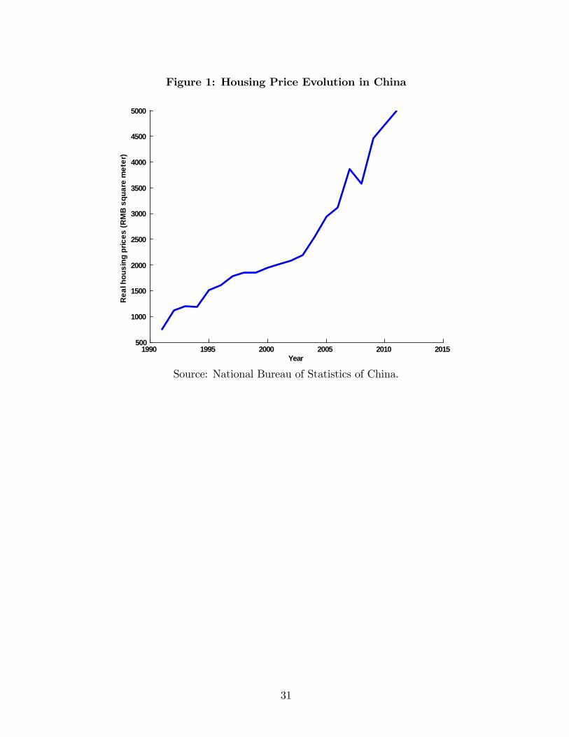
Figure 1: Housing Price Evolution in China

1990 1995 2000 2005 2010 2015500

1000

1500

2000

2500

3000

3500

4000

4500

5000R

eal h

ousi

ng p

rices

 (RM

B s

quar

e m

eter

)

Year

Source: National Bureau of Statistics of China.

31

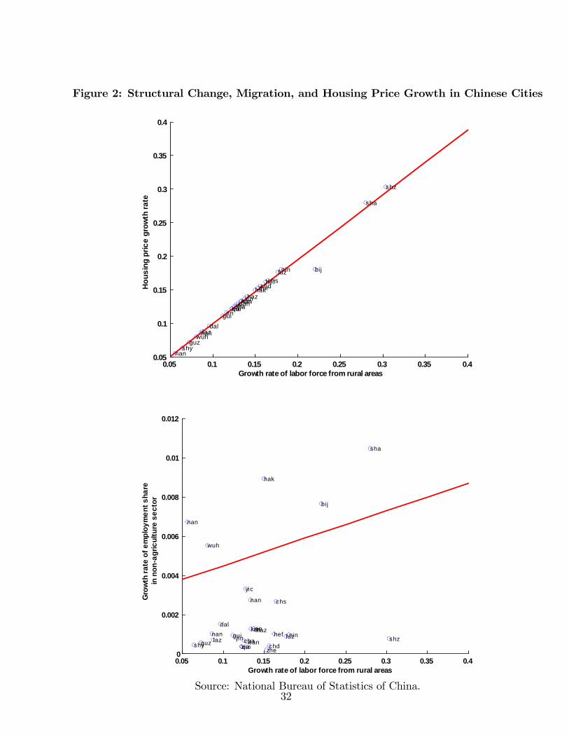
Figure 2: Structural Change, Migration, and Housing Price Growth in Chinese Cities

0.05 0.1 0.15 0.2 0.25 0.3 0.35 0.40.05

0.1

0.15

0.2

0.25

0.3

0.35

0.4

Growth rate of labor force from rural areas

Hou

sing

 pric

e gr

owth

 rate

bij

shy

dal

cha

sha

nan

haz

nin

heffuz

xianan

jinqin

zhe

wuh

chs

guz

shz

nan

hakchd

gui

kunxian

laz

xinyic

0.05 0.1 0.15 0.2 0.25 0.3 0.35 0.40

0.002

0.004

0.006

0.008

0.01

0.012

Growth rate of labor force from rural areas

Gro

wth

 rate

 of e

mpl

oym

ent s

hare

in n

on­a

gric

ultu

re s

ecto

r

bij

shy

dal

cha

sha

nan hazninhef fuz

xia

nan

jinqin zhe

wuh

chs

guzshz

nan

hak

chd

guikun

xianlaz

xin

yic

Source: National Bureau of Statistics of China.32

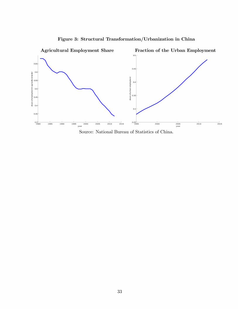
Figure 3: Structural Transformation/Urbanization in China

Agricultural Employment Share Fraction of the Urban Employment

1980 1985 1990 1995 2000 2005 2010 20150.3

0.35

0.4

0.45

0.5

0.55

0.6

0.65

y ear

shar

e of

 em

ploy

men

t in a

gricu

ltura

l sec

tor

1995 2000 2005 2010 20150.25

0.3

0.35

0.4

0.45

0.5

y ear

shar

e of

 urb

an e

mpl

oym

ent

Source: National Bureau of Statistics of China.

33

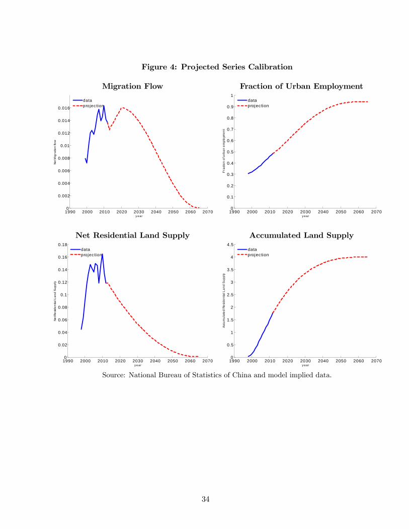
Figure 4: Projected Series Calibration

Migration Flow Fraction of Urban Employment

1990 2000 2010 2020 2030 2040 2050 2060 20700

0.002

0.004

0.006

0.008

0.01

0.012

0.014

0.016

y ear

Net

 Mig

ratio

n flo

w

dataprojec tion

1990 2000 2010 2020 2030 2040 2050 2060 20700

0.1

0.2

0.3

0.4

0.5

0.6

0.7

0.8

0.9

1

y ear

Frac

tion 

of u

rban

 em

ploy

men

t

dataprojection

Net Residential Land Supply Accumulated Land Supply

1990 2000 2010 2020 2030 2040 2050 2060 20700

0.02

0.04

0.06

0.08

0.1

0.12

0.14

0.16

0.18

y ear

Net R

esid

entia

l Lan

d Su

ppl

y

dataprojec tion

1990 2000 2010 2020 2030 2040 2050 2060 20700

0.5

1

1.5

2

2.5

3

3.5

4

4.5

y ear

Accu

mul

ated

 Res

iden

tial L

and 

Supp

ly

dataprojection

Source: National Bureau of Statistics of China and model implied data.

34

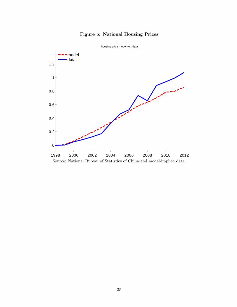
Figure 5: National Housing Prices

1998 2000 2002 2004 2006 2008 2010 2012

0

0.2

0.4

0.6

0.8

1

1.2

housing price model v.s. data

modeldata

Source: National Bureau of Statistics of China and model-implied data.

35

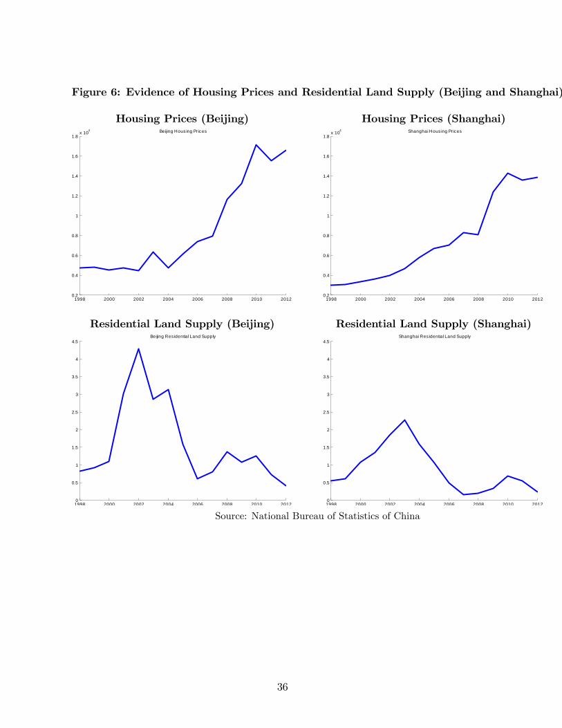
Figure 6: Evidence of Housing Prices and Residential Land Supply (Beijing and Shanghai)

Housing Prices (Beijing) Housing Prices (Shanghai)

1998 2000 2002 2004 2006 2008 2010 20120.2

0.4

0.6

0.8

1

1.2

1.4

1.6

1.8x  104 Beijing Hous ing Prices

1998 2000 2002 2004 2006 2008 2010 20120.2

0.4

0.6

0.8

1

1.2

1.4

1.6

1.8x  104 Shanghai Hous ing Prices

Residential Land Supply (Beijing) Residential Land Supply (Shanghai)

1998 2000 2002 2004 2006 2008 2010 20120

0.5

1

1.5

2

2.5

3

3.5

4

4.5Beijing Res idential Land Supply

1998 2000 2002 2004 2006 2008 2010 20120

0.5

1

1.5

2

2.5

3

3.5

4

4.5Shanghai Res idential Land Supply

Source: National Bureau of Statistics of China

36

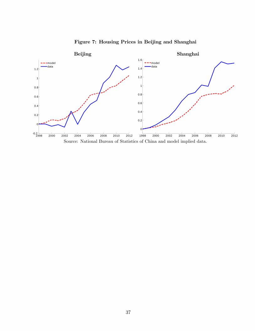
Figure 7: Housing Prices in Beijing and Shanghai

Beijing Shanghai

1998 2000 2002 2004 2006 2008 2010 2012­0.2

0

0.2

0.4

0.6

0.8

1

1.2

modeldata

1998 2000 2002 2004 2006 2008 2010 2012

0

0.2

0.4

0.6

0.8

1

1.2

1.4

1.6modeldata

Source: National Bureau of Statistics of China and model implied data.

37

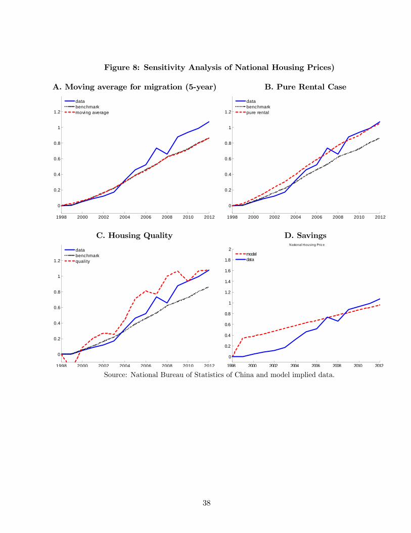
Figure 8: Sensitivity Analysis of National Housing Prices)

A. Moving average for migration (5-year) B. Pure Rental Case

1998 2000 2002 2004 2006 2008 2010 2012

0

0.2

0.4

0.6

0.8

1

1.2

databenchmarkmoving average

1998 2000 2002 2004 2006 2008 2010 2012

0

0.2

0.4

0.6

0.8

1

1.2

databenchmarkpure rental

C. Housing Quality D. Savings

1998 2000 2002 2004 2006 2008 2010 2012

0

0.2

0.4

0.6

0.8

1

1.2

databenchmarkquality

1998 2000 2002 2004 2006 2008 2010 2012

0

0.2

0.4

0.6

0.8

1

1.2

1.4

1.6

1.8

2National Hous ing Pric e

modeldata

Source: National Bureau of Statistics of China and model implied data.

38

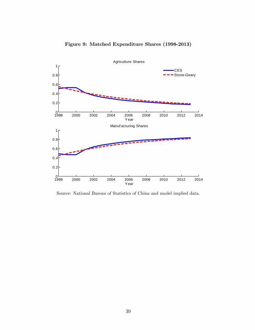
Figure 9: Matched Expenditure Shares (1998-2013)

1998 2000 2002 2004 2006 2008 2010 2012 20140

0.2

0.4

0.6

0.8

1

Year

Agriculture Shares

CESStone­Geary

1998 2000 2002 2004 2006 2008 2010 2012 20140

0.2

0.4

0.6

0.8

1Manuf acturing Shares

Year

Source: National Bureau of Statistics of China and model implied data.

39

Appendix A: An Overview of Development inChina (Not Intended for Publication)

This appendix summarizes development in China by focusing on the processes of struc-tural transformation and urbanization and their impact on the housing market. We begin bydocumenting some stylized facts and then discuss the importance of migration policies andthe deregulation of housing markets.

MIGRATION POLICIES

“The Third Plenary Session of the Eleventh Central Committee of the Communist Partyin China” in 1978 is widely believed to be the turning point in China’s development path.After this meeting, the Chinese economy began to transition from a centrally planned toa market-oriented economy. A key feature of the market economy is the introduction ofincentive mechanisms and the reduction of the monopoly power of state-owned enterprises.The encouragement of entrepreneurship stimulated unprecedented technological progress inall sectors. As labor productivity in the agricultural sector improved, surplus rural laborbecame available for urban employment. However, migration across regions remained heavilyregulated by the household registration system in China.The individual registration system, called “hukou”in Chinese, is required by law and still

in use, although it has changed significantly through the years. Each individual must have aregistration record, which offi cially identifies him or her as a resident of an area and includesidentifying information such as name, parents, spouse, and date of birth. In 1958, the Chinesegovernment offi cially promulgated this system to control the movement of people betweenurban and rural areas. Individuals were broadly categorized as “rural”or “urban”workers.A worker seeking to move from the country to an urban area for non-agricultural work had toapply through the relevant bureaucracies. The number of workers allowed to make such moveswas tightly controlled. Migrant workers needed six passes to work in provinces other thantheir own. People who worked outside their authorized domain or geographical area did notqualify for grain rations, employer-provided housing, or health care. There were additionalcontrols over education, employment, marriage, and so on. Although there have been changesover time, the hukou system is widely regarded as an impediment to economic development,and removing its restrictions is often viewed as crucial for fostering the migration needed tosupport industrialization. Indeed, China’s reform could not have begun without changes ineconomic institutions. China’s rural-urban migration history can be divided into three stagesbased on changes in the central government’s migration policy that began in 1978.

1. Steady stage (1978-1983): During this early stage of reform, all economic changes werestill under probation and the key theme was slow progress. Because of the continued emphasis

40

on agricultural self-suffi ciency, most of the migration flows were within rural areas. Of theabout 14 to 23 million migrants during this time, only 1 million migrated across provinces,which was less than 0.1 percent of the total population. Although agricultural productivityadvanced during this period, those workers who left their farmland moved mainly to localtownship enterprises. This shift created a phenomenon called “leave the land without leavinghome.”Workers left the farm labor force but still resided in rural areas.

2. Gradual growth stage (1984-1994): As agricultural productivity continued to in-crease, more rural workers left the agricultural sector, and local township enterprises couldnot accommodate these surplus laborers. The leave-the-land-without-leaving-home mode re-quired a breakthrough. As a result, to meet the needs of economic development, policiesrestricting migrants from moving from rural areas to cities were mitigated. In 1984, theGeneral Offi ce of the State Council published a new document on the settlement of ruralmigrants in urban areas, making it easier to migrate to the city. This reform of the hukousystem drastically improved the employment opportunities for rural workers. Cities grew asthe mantra gradually changed to “leave both land and home.”Meanwhile, instead of movingmainly to small towns, as in the early 1980s, rural workers started moving to bigger cities,including megalopolises such as Beijing and Shanghai. From 1984 to 1994, rural-urban mi-gration generally kept a steady pace. The average number of rural migrants moving acrossprovinces increased to 3.2 million per year, three times as many as in the previous stage.

3. Highly active stage (1995-2000): Population movement in China became highlyactive beginning in 1995. Over the period 1995 to 2000, the total number of rural migrantsmoving across provinces grew from 3.5 to 10 million. Growth in this stage was the result ofthree important policy changes:

• Deng Xiaoping southern tour: With the world-famous speech given by Deng Xi-aoping in 1992 and the reforms that followed, the Chinese economy boomed. Theeastern coastal area experienced unprecedented economic growth, and a number ofspecial economic development zones were built, which attracted many foreign enter-prises and investment. This growth created more jobs in cities in these zones, inducingmore workers to leave rural areas.

• Abandonment of the centrally planned food and housing allocation system:Prior to 1995, the central government generally controlled the allocation of food andhousing among citizens; workers without a legal permit to live in the city were not ableto obtain food and housing. Even though they could afford them because there wereessentially no markets for them to trade in. The establishment of markets for basicliving necessities such as food and housing greatly facilitated the entry of rural peopleinto the city.

41

• Temporary work permits in large cities: Toward the end of the 1990s, migrationaccelerated as a result of policies that allowed migrants temporary permits to work inlarge cities. For instance, in 1997 the General Offi ce of the State Council permittedsome big cities, such as Shanghai and Guangzhou, to print “blue household registra-tion cards”or “temporary permits”for rural workers according to the city’s needs. Itis estimated that in Zhejiang province, one of the richest provinces in China, the ruralmigrant population reached 1.9 million from 1998 to 2001. Some provinces abolishedall offi cial restrictions between rural and urban areas by declaring everyone a “citizen ofthat province”with equal treatment under the same set of policies. The salient featureof the rural-urban migration in this period was likely the concentration of economicdevelopment in the eastern coastal areas, which had faster economic growth and higherwages.

THE DEVELOPMENT OF THE HOUSING MARKET IN CHINA

After the 1978 Central Committee the Communist Party sessions, urban housing reformsbecame a major focus of the economic transformation. The central government has beenvery cautious in applying new reform policies in the public housing sector and has conductedout various experiments to commercialize the existing urban public housing. All land (urbanand rural) is owned by the state, where developers can lease the rights to use the land fromthe government.According to the 2010 Population Census, the reported statistic for the national home-

ownership rate in China is around 85 percent. The national average roughly captures a closeto 100 percent homeownership rate in rural areas (close to 50 percent of the householdssurveyed) with a relatively lower rate in large cities. More specifically, the homeownershiprates in the two largest cities, Beijing and Shanghai, were close to 60 percent (with severalprovinces above 80 percent). These numbers are substantially higher than some of the largestcities in the United States (i.e., cities like Los Angeles and New York have home ownershiprates below 40 percent). In addition to a high homeownership rate, Deng, Gyourko, and Wu(2015) use the Urban Household Survey in nine provinces from 2002 to 2009 to show thatmost Chinese cities have a modest vacancy rate. In particular, the vacancy rate in Beijingis about 5 percent, with the highest vacancy rate in Zhejiang province at only 7.9 percent.The high homeownership and low vacancy rate are considered in designing the structure ofthe model.The path of urban housing and land market reforms can be divided into three stages:

1. Probation and experimentation stage (1978-1988): An April 1980 speech by DengXiaoping announced urban housing reform. He pointed out specifically that (i) urban resi-dents should be allowed to purchase houses (old or new) and (ii) public housing rents should

42

be adjusted in accordance with rising construction costs (which encouraged home buyingrather than renting). These policies symbolized a major shift in long-standing policies forthe public housing system. Following Xiaoping’s directive, limited experiments were con-ducted in selected cities between 1980 and 1998, focused on reorganizing housing productionand promoting sales of public housing to ensure a suffi cient return on housing investment.These experiments included encouraging new housing sales for building costs alone, subsidiz-ing public housing sales, and increasing public housing rents steadily each year to promotesales.These policies, however, provided little incentive for private or other forms of housing

investment. In the centrally planned economy, housing investments were provided solely bythe state through a redistribution process. During economic reform, the central governmenttried to adopt policies to decentralize managerial power and introduce market functionsinto the economy. With no experience with a market economy, however, the majority ofSOE became less competitive than the emerging collectively owned and private enterprises.Consequently, public housing subsidized by the central government could not keep up withthe increasing demand for public housing. Although the private sector increased steadily eachyear, there was not enough incentive for the private sector to move toward urban housinginvestment because of the risk. Therefore, private investment in housing production was lowand insuffi cient total investment in urban housing was inevitable. The market for land useis nonexistent and developers purchase the rights of use directly from the government.

2. Further urban housing reform (1988-1998): At the beginning of 1988, the centralgovernment held the first national housing reform conference in Beijing. It was agreed in thatconference that housing reform could lead to great economic and social benefits and that abigger systematic housing reform plan was necessary. The major resolutions of the conferencewere summarized in a document that was updated and published in 1991. This documentmarked a turning point in urban housing reform, from pilot tests and experiments in selectedcities to implementation in all urban areas. Although there were no significant changes inthe overall objectives, this was the first resolution to recognize ownership of private housingpurchased from the public sector. Purchasers of public housing had two options: (i) Paythe market price and have complete ownership of the unit or (ii) pay the “standard price”(subsidized price) for partial ownership. This reform conveyed the message that the urbanhousing sector would eventually rely on market forces rather than central planning.Although a less than fully privatized housing market had been established, most partic-

ipants in that market at that time were employers, not individual buyers. With differentinterests and more independent policies, employers and local governments purchased housesand then provided them to their employees at rents substantially below market rates. Thus,the overwhelming majority of urban residents lived in public housing that was also tied totheir employment. As a consequence, there was less incentive for urban residents to purchase

43

housing units.

3. Current stage of urban housing policies (1998-present): In July 1998, the newState Council adjusted the housing policy and issued an offi cial document. One major changewas the termination of material distribution of housing at the end of 1998, which was com-pletely replaced by monetary distribution. According to the new plan, no newly built unitswere to be allotted. The new policy symbolized the end of the existing public housing sys-tem, with the ultimate goal of fully commercializing the housing market. Nonetheless, thegovernment continued to provide cheap-rent housing for the lowest-income households, butthe average floor space per person could not exceed 60 percent of the local average. Individ-uals who did not qualify for these government programs had to purchase or rent houses inthe private market. During this period public land auctions were institutionalized in 2002and became widespread across all cities. By August 31, 2004, all urban land leasing saleswere required to be through public auctions with Internet posting to the public. Local landbureaus remained in charge of annual allocation of land plots for development, the associatedregulations (including the floor area ratios), and the types and reservation prices for auctions.In response to the financial tsunami, the Chinese government implemented two additional

policies with the objective of cooling off the housing boom. The main regulatory changeswere the restriction on owning multiple housing units (including regulations that required aminimum down payment of 60 percent), mortgage restrictions on nonlocal households, andsales restrictions in second- and third-tier cities to only local or migrant households. Otherhousing policies aimed at slowing housing price growth included higher property tax ratesin Shanghai and Chongqing as well as building and running public rental housing. Suchtightened housing policy was recently reverted during the first quarter of 2015 to revive thesluggish growth of the housing market.

Appendix B: Technical Companionconsol Mortgage: The consol fixed-rate mortgage (FRM) considered in our paper possessesthe following properties:

Proposition 1: Consol FRM has zero amortization, bt = bt+1.

Proof: A mortgage payment contains two parts: the amortization and the interest payment.Amortization is defined as the difference between today’s debt and tomorrow’s debt:

mt = at + it,

at = bt − bt+1.

The debt level in period 0 is b0 = (1− φ)q0h, and the interest payment in period 1 is

i1 = (1

β− 1)b0.

44

Assume the mortgage payment decreases at a constant rate g over time. The absence ofarbitrage condition implies

(1− φ)q0h =∞∑t=1

βtd1(1− g)t.

We can solve d1 as follows:

d1 = (1− φ)q0h1− β(1− g)

β(1− g).

Therefore, amortization in period 1 can be derived as

a1 = d1 − i1 = g(1− φ)q0h.

Under a constant debt repayment scheme, amortization is zero.

Proposition 2: The down payment constraint is always binding.

Proof: Consider parameter values {Amt } such that there “reverse migrations”from the cityto the rural area are not optimal. In this case, the relevant optimization problem becomes

V Ct (ε, bτ ) = maxU(cmt , c

ft , ht) + βV C

t+1(ε, bτ ),

s.t. ptcft + cmt + bτr

∗ = wmt .

Rewriting the optimization problem sequentially gives

max∞∑t=0

βtU(cmτ+t, cfτ+t, hτ ),

s.t. cmτ + pτcfτ + qτhτ = wmτ + bτ ,

cmt+τ + pt+τcft+τ + bτr

∗ = wmt+τ , ∀t > 1,

bτ ≤ (1− φ)qτhτ .

The Lagrangian has the form

L = U(cmτ , cfτ , hτ ) + λ0(w

mτ + bτ − cmτ − pτcfτ − qτhτ )+

∞∑t=1

βt[U(cmτ+t, cfτ+t, hτ ) + λt(w

mt+τ − cmt+τ − pt+τc

ft+τ − bτr∗) + γ((1− φ)qτhτ − bτ ).

45

First-order conditions with respect to{cmt+τ , c

ft+τ

}and bτ give the following:

cmt+τ : U′

1(cmτ+t, c

fτ+t, hτ ) = λt,

hτ : U′

3(cmτ , c

fτ , hτ )− λ0qτ +

∞∑t=1

βtU′

3(cmτ+t, c

fτ+t, hτ ) + γ(1− φ)qτ = 0,

bτ : λ0 −∞∑t=1

βtλtr∗ − γ = 0.

When γ > 0, the borrowing constraint will be binding. Collecting the terms gives

γ = λ0 −∞∑t=1

βtλtr∗ = U

′

1(cmτ , c

fτ , hτ )[1− r∗

∞∑t=1

βtU′1(c

mτ+t, c

fτ+t, hτ )

U′1(c

mτ , c

fτ , hτ )

].

Therefore, γ is positive as long as the utility function is strictly increasing, weakly concavein the consumption component, and the discount factor satisfies β ≤ 1

1+r∗ .

46

Data Appendix C: Data Sources andDefinitions

Employment and Population: The source for the urban and agricultural employmentdata come from China Statistical Yearbook. The statistics cover all agencies and units pro-viding employment services and job centers. The scope of statistics on private enterprises andself-employed individuals covers the whole country, which includes 31 provinces, autonomousregions and municipalities directly under the central government. The number of employedpeople in urban areas does not include those who had left their working units and kept theirlabor contract/employment relation unchanged since 1998. The share of agriculture in GDPis from primary industry measures.

Migration Flow: The migration charts in Figure 2 are obtained from the City StatisticalYearbook. The labor force from rural areas is measured as the number of workers holdingagricultural hukou.

Housing Prices: The data source is China Statistical Yearbook. Nominal housing pricesare calculated using total sales of residential buildings divided by the floor space of residen-tial buildings. Real housing prices are calculated by deflating nominal housing prices by theconsumer price index in urban areas.

Residential Land Supply: The data source is China Statistical Yearbook. The flow ofresidential land supply is land purchased in the current year. The measure of total urbanland area is constructed from data on area of land used for urban construction.

City-Level Data: Housing price data for both Beijing and Shanghai are from ChinaStatistical Yearbook 1998-2012 and are deflated using the consumer price index in eachcity. The simulated housing price is based on a calibrated multiple-city model, which mimicsseveral stylized facts of the Chinese economy as well as migration patterns into each city.The flow of residential land supply is land purchased in the current year. We use the area ofland used for urban construction to measure the total urban land area for both cities.

47