multidimensional poverty measurement and analysis: chapter
TRANSCRIPT

Oxford Poverty & Human Development Initiative (OPHI) Oxford Department of International Development Queen Elizabeth House (QEH), University of Oxford
* Sabina Alkire: Oxford Poverty & Human Development Initiative, Oxford Department of International Development, University of Oxford, 3 Mansfield Road, Oxford OX1 3TB, UK, +44-1865-271915, [email protected] ** James E. Foster: Professor of Economics and International Affairs, Elliott School of International Affairs, 1957 E Street, NW, [email protected]. *** Suman Seth: Oxford Poverty & Human Development Initiative (OPHI), Queen Elizabeth House (QEH), Department of International Development, University of Oxford, UK, +44 1865 618643, [email protected]. **** Maria Emma Santos: Instituto de Investigaciones Económicas y Sociales del Sur (IIES,), Departamento de Economía, Universidad Nacional del Sur (UNS) - Consejo Nacional de Investigaciones Científicas y Técnicas (CONICET), 12 de Octubre 1198, 7 Piso, 8000 Bahía Blanca, Argentina. Oxford Poverty and Human Development Initiative, University of Oxford. [email protected]; [email protected]. ***** Jose Manuel Roche: Save the Children UK, 1 St John's Lane, London EC1M 4AR, [email protected]. ****** Paola Ballon: Assistant Professor of Econometrics, Department of Economics, Universidad del Pacifico, Lima, Peru; Research Associate, OPHI, Department of International Development, Oxford University, Oxford, U.K, [email protected].
This study has been prepared within the OPHI theme on multidimensional measurement.
OPHI gratefully acknowledges support from the German Federal Ministry for Economic Cooperation and Development (BMZ), Praus, national offices of the United Nations Development Programme (UNDP), national governments, the International Food Policy Research Institute (IFPRI), and private benefactors. For their past support OPHI acknowledges the UK Economic and Social Research Council (ESRC)/(DFID) Joint Scheme, the Robertson Foundation, the John Fell Oxford University Press (OUP) Research Fund, the Human Development Report Office (HDRO/UNDP), the International Development Research Council (IDRC) of Canada, the Canadian International Development Agency (CIDA), the UK Department of International Development (DFID), and AusAID.
ISSN 2040-8188 ISBN 978-19-0719-471-9
OPHI WORKING PAPER NO. 84
Multidimensional Poverty Measurement and Analysis: Chapter 3 – Overview of Methods for Multidimensional Poverty Assessment
Sabina Alkire*, James E. Foster**, Suman Seth***, Maria Emma Santos***, Jose M. Roche**** and Paola Ballon*****
January 2015
Abstract This chapter presents a constructive survey of the major existing methods for measuring multidimensional poverty. Many measures were motivated by the basic needs approach, the capability approach, and the social inclusion approach among others. This chapter reviews Dashboards, the composite indices approach, Venn diagrams, the dominance approach, statistical approaches, fuzzy sets, and the axiomatic approach. The first two methods (dashboard and composite indices) are implemented using aggregate data from different sources ignoring the joint distribution of deprivations The other methods reflect the joint distribution and are implemented using data in which information on each dimension is available for each unit of analysis. After outlining each method, we provide a critical evaluation by discussing its advantages and disadvantages.

Alkire, Foster, Seth, Santos, Roche and Ballon 3: Overview of Methods
The Oxford Poverty and Human Development Initiative (OPHI) is a research centre within the Oxford Department of International Development, Queen Elizabeth House, at the University of Oxford. Led by Sabina Alkire, OPHI aspires to build and advance a more systematic methodological and economic framework for reducing multidimensional poverty, grounded in people’s experiences and values.
The copyright holder of this publication is Oxford Poverty and Human Development Initiative (OPHI). This publication will be published on OPHI website and will be archived in Oxford University Research Archive (ORA) as a Green Open Access publication. The author may submit this paper to other journals.
This publication is copyright, however it may be reproduced without fee for teaching or non-profit purposes, but not for resale. Formal permission is required for all such uses, and will normally be granted immediately. For copying in any other circumstances, or for re-use in other publications, or for translation or adaptation, prior written permission must be obtained from OPHI and may be subject to a fee.
Oxford Poverty & Human Development Initiative (OPHI) Oxford Department of International Development Queen Elizabeth House (QEH), University of Oxford 3 Mansfield Road, Oxford OX1 3TB, UK Tel. +44 (0)1865 271915 Fax +44 (0)1865 281801 [email protected] http://www.ophi.org.uk
The views expressed in this publication are those of the author(s). Publication does not imply endorsement by OPHI or the University of Oxford, nor by the sponsors, of any of the views expressed.
Keywords: Multidimensional poverty measures, dashboard approach, composite indices, Venn diagrams, dominance approach, statistical approaches, fuzzy sets approach, axiomatic approach.
JEL classification: B40, I32.
Acknowledgements: We received very helpful comments, corrections, improvements, and suggestions from many across the years. We are also grateful for direct comments on this working paper from Tony Atkinson, Achille Lemmi, Betti Gianni, Conchita D'Ambrosio, Enrica Chiappero Martinetti, Frances Stewart, Jacques Silber, Jaya Krishnakumar, Jean-Yves Duclos, Francois Bourguignon.
Citation: Alkire, S., Foster, J. E., Seth, S., Santos, M. E., Roche, J. M., and Ballon, P. (2015). Multidimensional Poverty Measurement and Analysis, Oxford: Oxford University Press, ch. 3.

Alkire, Foster, Seth, Santos, Roche and Ballon 3: Overview of Methods
OPHI Working Paper 84 www.ophi.org 1
3 Overview of Methods for Multidimensional Poverty Assessment
Since the early twentieth century, poverty measurement has predominantly used an
income approach.1 Yet the recognition of poverty as a multidimensional phenomenon is
not new. Since the mid-1970s at least, empirical analyses have considered various non-
monetary deprivations that the poor experience, complementing monetary measures.
Conceptually, many analyses were motivated by the basic needs approach, the capability
approach, and the social inclusion approach among others. A number of methodologies
have emerged to assess poverty from a multidimensional perspective. This chapter
presents a constructive survey of the major existing methods. Each section describes a
methodology; identifies the data requirements, assumptions, and choices made during
measurement design; and lists the types of problems it best analyses—as well as its
challenges. A reader, upon reading this chapter and the next, should have a clear
overview of existing methodologies as well as the Alkire–Foster measures, their
applicability, and insights. The AF methodology, which we focus on from Chapter 5
onwards, draws together the axiomatic and counting approaches explicitly, yet builds
upon insights from other methodologies too. So a further motivation for this chapter is
to acknowledge intellectual debts to many others in this fast-moving field.
This chapter reviews the dashboard approach, the composite indices approach, Venn
diagrams, the dominance approach, statistical approaches, fuzzy sets, and the axiomatic
approach. Some techniques within each approach can be used with ordinal as well as
cardinal data. These methods can be grouped into two broad categories. One category
encompasses methods that are implemented using aggregate data from different sources.
These thus ignore the joint distribution of deprivations and are ‗marginal measures‘ as
defined in Chapter 2. The second category encompasses methods that reflect the joint
distribution and thus are implemented using data in which information on each
dimension is available for each unit of analysis.
Among marginal methods, dashboards assess each and every dimension separately but a
priori impose no hierarchy across these dimensions. Also dashboards do not identify who
is to be considered multidimensionally poor. Thus the dashboard method does not
indicate the direction and extent of changes in overall poverty. Composite indices have
1 This is evidenced in the seminal surveys of Booth (1894, 1903), Rowntree (1901), and Bowley and Burnett-Hurst (1915) conducted in specific cities in the UK.

Alkire, Foster, Seth, Santos, Roche and Ballon 3: Overview of Methods
OPHI Working Paper 84 www.ophi.org 2
‗the powerful attraction of a single headline figure‘ (Stiglitz et al. 2009) but like the
dashboard approach, have the disadvantage of missing a key aspect of multidimensional
poverty assessment: the joint distribution of deprivations. Dashboards and composite
indexes are discussed in section 3.1.
Within the second group of methods, Venn diagrams, outlined in section 3.2, graphically
represent the joint distribution of individuals‘ deprivations in multiple dimensions. Yet
they become difficult to read when more than four dimensions are used and do not per
se contain a definition of the poor. The dominance approach, covered in section 3.3,
enables us to state whether a country or region is or is not unambiguously less poor than
another with respect to various parameters and functional forms, but it becomes
empirically difficult to implement beyond two or more dimensions. It also shares with
the Venn diagrams the disadvantage of not offering a summary measure. Moreover, the
dominance approach only ranks regions or poverty levels from different periods
ordinally; it does not permit a cardinally meaningful assessment of the extent of the
differences in poverty levels.
Statistical approaches (section 3.4) comprise a wide range of techniques. Techniques such
as principal component analysis and multiple correspondence analysis extract
information on the correlation or association between dimensions to reduce the number
of dimensions; other techniques, such as cluster analysis, identify groups of people who
are similar in terms of their joint deprivations. These and other methods, such as factor
analysis and structural equation models, can be used to construct overall indices of
poverty. It should be noted that even when overall indices of poverty can be obtained,
because statistical techniques rely on the particular dataset used, it may be difficult to
make intertemporal and cross-country comparisons.
The fuzzy set approach, outlined in section 3.5, also falls within the second category of
techniques and builds on the idea that there is ambiguity in the identification of who is
deprived or poor. Thus, instead of using a unique set of deprivation cut-offs for
identification, it uses a band of deprivation cut-offs for each dimension. A person falling
above the band is identified as unambiguously non-deprived, whereas a person falling
below the band is identified as unambiguously deprived. Within the band of ambiguity, a
membership function is chosen to assign the degree to which the person is deprived.
Fuzzy sets are used to construct a summary measure, and they may address joint
Alkire, Foster, Seth, Santos, Roche and Ballon 3: Overview of Methods
OPHI Working Paper 84 www.ophi.org 3
deprivations. The challenge lies in selecting and justifying the membership function, as
well as in communicating results.
It is worth noting that the measurement methods just mentioned are not regularly
scrutinized according to the set of properties stated in Chapter 2. The measures
developed within the axiomatic approach discussed in section 3.6—our last method—
articulate precisely some of the properties for multidimensional poverty measurement
they satisfy. Measures that clearly specify the axioms or properties they satisfy enable the
analyst to understand the ethical principles they embody and to be aware of the direction
of change they will exhibit under certain transformations. Note that the appropriateness
of axiomatic measures critically depends on whether their properties are essential or
useful given the purpose of measurement.
3.1 Dashboard of Indicators and Composite Indices
A starting point for measuring the multidimensionality of poverty is to assess the level of
deprivation in dimensions separately, in other words, to apply a ‗standard unidimensional
measure to each dimension‘ (Alkire, Foster, and Santos 2011). This is the so-called
dashboard approach, which consists of considering a set of dimensional deprivation
indices ( ; )jj jP x z , defined in section 2.2.2. The dashboard of indicators, denoted by DI ,
is a d -dimensional vector containing the deprivation indices of all d dimensions: 1
1 1( ( ; ), , ( ; } dd dDI P x z P x z .)).
Writing from within a basic needs approach framework, Hicks and Streeten proposed the
use of dashboards: ‗as a first step, it might be useful to define the best indicator for each
basic need …. A limited set of core indicators covering these areas would be a useful
device for concentrating efforts‘ (1979: 577). 2 A prominent implementation of a
dashboard approach has been the Millennium Development Goals: a dashboard of 49
indicators was initially defined to monitor the eighteen targets to achieve the eight goals.
Improvements in different aspects of poverty are evaluated with independent indicators,
such as the proportion of people living below $1.25 a day, the fraction of children under
5 years of age who are underweight, the child mortality rate, the share of seats held by
women in single or lower houses of national parliaments, and so on. This provides a rich
and variegated profile of a population‘s achievements across a spectrum of dimensions
2 See also Ravallion (1996, 2011b).

Alkire, Foster, Seth, Santos, Roche and Ballon 3: Overview of Methods
OPHI Working Paper 84 www.ophi.org 4
and their changes over time. Furthermore, in many cases the indicators can be
decomposed to illuminate disparities.
Observe that the different indicators in a dashboard are not necessarily based on the
same reference population (section 2.2.2). In our notation, the jn population may be
different for each j dimension. For example, the indicator of the proportion of people
living below the $1.25-a-day poverty line reflects the entire population, whereas the
indicator of the fraction of children under 5 years of age who are underweight is based
only on children under 5 years old. In turn, the share of seats held by women in single or
lower houses of national parliaments reflects only the men and women in the single or
lower houses of national parliaments. The different reference populations reflected in the
indicators of a dashboard may be ‗disjoint‘ (that is, they have no people in common) or
overlapping (they have people in common).
An example of disjoint indicators is child malnutrition (computed using information for
children under 5 years of age) and share of seats held by women in parliament (computed
using information for men and women in the single or lower houses of national
parliaments). If the indicators pertain to disjoint populations, there seems to be no need
to consider joint deprivations. However, even in this case, joint deprivations could be
relevant if the disjoint populations have something in common—such as belonging to
the same household. Under such circumstances, the deprivation experienced by one
individual (for example, a child who is malnourished) can affect others (like her mother).
This is known as an intra-household negative externality. Thus, ignoring the joint
distribution of a composite unit of analysis (households in the example) may obscure
important aspects of poverty. An example of indicators with overlapping populations is
the proportion of people living on less than $1.25 a day and the percentage of people
without adequate sanitation. In this case, because both deprivations can be experienced
by both groups of people, the information on the extent to which those living on less
than $1.25 a day are also deprived in sanitation and vice versa may be relevant.
Dashboards have the advantage of broadening the set of considered dimensions, offering
a rich amount of information, and potentially allowing the use of the best data source for
each particular indicator and for assessing the impact of specific policies (such as
nutritional or educational interventions). However, they have some significant
disadvantages. First of all, dashboards do not reflect joint distribution of deprivations
across the population and precisely because of that they are marginal methods. Recall the

Alkire, Foster, Seth, Santos, Roche and Ballon 3: Overview of Methods
OPHI Working Paper 84 www.ophi.org 5
example presented in Table 2.2 on section 2.2.3, which used two deprivation matrices
with equal marginal distributions but different joint distributions, one in which each of
the four persons in the distribution is deprived in exactly one dimension and another
distribution in which one person is deprived in all dimensions and three persons
experience zero deprivations. A dashboard of dimensional deprivation indices for these
four dimensions would indicate that the level of deprivation in each of the four
dimensions is the same in both distributions.
Technically, a dashboard could also include a measure of correlation or association
between every pair of dimensions, which may account for the joint distribution in some
restricted sense. However, a large number of indicators in dashboards require an even
larger number of pairwise correlations to be reported, which is definitely expected to
increase complexity. Perhaps that is why such kinds of correlation indicators are not in
practice included in dashboards. Even if bivariate associations/correlations are reported,
they still do not account for the underlying multivariate joint distribution, and thus
remain silent in identifying who the poor are. Secondly and relatedly, ‗…dashboards
suffer because of their heterogeneity, at least in the case of very large and eclectic ones,
and most lack indications about … hierarchies among the indicators used. Furthermore,
as communications instruments, one frequent criticism is that they lack what has made
GDP a success: the powerful attraction of a single headline figure that allows simple
comparisons of socio-economic performance over time or across countries‘ (Stiglitz et al.
2009: 63).
One way to overcome this heterogeneity and communications challenge is through
composite indices. A composite index (CI ) is a function 1 2
1 1 2 2: ( ; ) ( ; ) ( ; )u u}u odd dCI P x z P x z P x z that converts d deprivation indices
(which one may consider in a dashboard) into a real number. An example of an
aggregation function used in composite indices is the family of generalized means of
appropriate order E , introduced in section 2.2.5.
There is a burgeoning literature on composite indices of poverty or well-being.3 Well-
known indices include the Physical Quality of Life Index (Morris 1978), the Human
Development Index (HDI) (Anand and Sen 1994), the Gender Empowerment Index
3 For further discussions on composite indices see Nardo et al. (2008), Bandura (2008), Alkire and Sarwar (2009), Maggino (2009), Fattore, Maggino, and Colombo (2012), Fleurbaey and Blanchet (2013), and Santos and Santos (2013).

Alkire, Foster, Seth, Santos, Roche and Ballon 3: Overview of Methods
OPHI Working Paper 84 www.ophi.org 6
(GEM) (UNDP 1995), and, within poverty measurement, the Human Poverty Index
(HPI) (Anand and Sen 1997). These indices have been published in the global Human
Development Reports for several years.4 A prominent policy index is the official EU-2020
measure of poverty and social exclusion, which uses a union counting approach across
three dimensions: income poverty, joblessness, and material deprivation (Hametner et al.
2013).
Composite indices, like dashboards, can capture deprivations of different population
subgroups and can combine distinct data sources. In contrast to dashboards, they impose
relative weights on indicators, which govern trade-offs across aggregate dimensional
dimensions. Such normative judgements are very demanding (Chapter 6) and have been
challenged (Ravallion 2011b). In practice, they have catalysed expert, political, or public
scrutiny of and debate about these trade-offs, facilitating a process of public reasoning as
recommended by Sen (2009).
Like dashboards, composite indices do not reflect the joint distribution of deprivations.
In fact, a composite index of the four dimensional deprivations presented in Table 2.2
would combine these indices with some aggregation formula, but would show the level
of overall deprivation in the two distributions as being identical. In other words, both the
dashboard and composite indices are insensitive to the degree of simultaneous
deprivations.
Moreover, composite indices like dashboards remain silent to one of the basic steps of
poverty measurement: identification of the poor. Even when a composite index is
constructed by considering all deprivations within a society in the selected dimensions, it
fails to identify the set of the poor Z within the society. It may appear that, when the
base population is the same for all considered dimensions, such composite indices follow
the union criterion to identification as they consider all deprivations, but this notion is
not correct because the identification of all deprivations does not ensure the
identification of the set of poor. In fact as long as there is at least one person
experiencing more than one deprivation, counting the deprived in each dimension would
4 The HDI has been published since the first Human Development Report in 1990 (UNDP 1990). The GEM was published between 1995 and 2009; in 2010, it was replaced by the Gender Inequality Index (GII), which is based on the methodology proposed by Seth (2009). The HPI was published between 1997 and 2009; in 2010, it was replaced by the Multidimensional Poverty Index (Alkire and Santos 2010), when the IHDI or Inequality Adjusted HDI was added (Alkire and Foster 2010).

Alkire, Foster, Seth, Santos, Roche and Ballon 3: Overview of Methods
OPHI Working Paper 84 www.ophi.org 7
lead to a double counting of the number of the ‗union poor‘ (see Bourguignon and
Chakravarty 2003: 28–9). Thus neither dashboards nor composite indices can answer the
questions: Who is poor? How many poor people are there? How poor are they? (Alkire,
Foster, and Santos 2011). In sum, the dashboard approach and composite indices
represent important tools for understanding poverty based on multiple dimensions, and
can be used with multiple data sources covering different reference populations.
However, their inability to capture the joint distribution of multiple dimensions and to
identify what proportion of the population are poor make them limited tools for
multidimensional poverty measurement and analysis. 5 In the following sections, we
introduce approaches that address the joint distribution of deprivations.
3.2 Venn Diagrams
Venn diagrams are a diagrammatic representation that shows all possible logical relations
between a finite collection of sets. The name of Venn diagrams refers to John Venn who
formally introduced the tool (Venn 1880), although the tool pre-existed and was
known—as Venn himself mentions—as Eulerian circles (in fact, although Euler used
them, there were uses of similar representations even before Euler).6 Venn diagrams
consist of a collection of closed figures, such as circles and ellipses, that include, exclude,
or intersect one another such that each compartment is associated with a class.7
3.2.1 The Methodology and Applications
Applied to the analysis of multidimensional poverty measurement, the interior of each
closed figure in a Venn diagram can be used with a set of indicators and associated
deprivation cut-offs to represent the number of people who are deprived in a certain
dimension. Naturally, the exterior of each closed figure can be used to represent the
number of people who are non-deprived in the same dimension. Note that these two
groups—deprived and non-deprived—within each dimension are mutually exclusive and
collectively exhaustive with respect to the considered population. The intersections
between the closed figures show the extent to which deprivations in different dimensions
5 Seth (2010) pointed out the key difference between composite indices and multidimensional indices, which is that the former do not capture the joint distribution of achievements. 6 Venn (1880) does not refer to the diagrams as ‗Venn diagrams‘. Lewis (1918) first named the tool as a Venn diagram. 7 ‗... any closed figure will do as well ... all that we demand of it ... is that it shall have an inside and an outside, so as to indicate what does and what does not belong to the class‘ (Venn 1880: 6).

Alkire, Foster, Seth, Santos, Roche and Ballon 3: Overview of Methods
OPHI Working Paper 84 www.ophi.org 8
overlap, that is, the number of people who are jointly deprived in the overlapping
dimensions in a particular society.
Table 3.1 Joint distribution of deprivation in two dimensions
Dimension 2 Non-deprived Deprived Total
Dimension 1 Non-deprived 00n 01n 0�n Deprived 10n 11n 1�n
Total 0�n 1�n n
When there are only two dimensions, a Venn diagram provides a diagrammatic
representation of a 2u2 contingency table, introduced in section 2.2.3. Here we reproduce
Table 2.1 as Table 3.1 in order to visually link it to Figure 3.1 below. Figure 3.1 contains
the same pattern of joint distribution as Table 3.1, but in a Venn diagram. The circle with
a darker shade to the left denotes the number of people who are deprived in Dimension
1, whereas the circle with a lighter shade denotes those who are deprived in Dimension
2. In this example, without a loss of generality, we assume that more people are deprived
in Dimension 2 than in Dimension 1; hence, the circle corresponding to Dimension 2 is
larger than that of Dimension 1. The intersection of the two circles represents the
number of people who experience deprivations in both dimensions, 11, n and is larger or
smaller according to the extent of overlap The diagram also represents the number of
people deprived in the first but not in the second dimension, 10n , and those deprived in
the second but not the first dimension, 01n . If some people are deprived in each
dimension but no one is jointly deprived, the two circles do not intersect.
Figure 3.1 Venn diagram of joint distribution of deprivations in two dimensions
The Venn diagram is particularly useful when two to four dimensions are involved,
because the visual representation is easy to interpret. A three-dimension Venn diagram is

Alkire, Foster, Seth, Santos, Roche and Ballon 3: Overview of Methods
OPHI Working Paper 84 www.ophi.org 9
shown in Figure 3.2. The diagram depicts the frequencies for all the possible
combinations of deprivations using the notation 1 2 3j j jn , such that 1 jL signals deprivation
in dimension jL and 0 jL signals non-deprivation in dimension jL for all 1,2,3 L . Thus,
for example, 111n in the intersection of the three circles denotes the number of people
who are deprived in all three dimensions, 010n denotes the number of people who are
deprived in the second dimension only, and so on for other combinations.
Figure 3.2 Venn diagram of joint distribution of deprivations in three dimensions
In empirical work, the Venn diagram has been used as an exploratory tool to understand
the overlapping deprivations in various dimensions and to draw attention to mismatches
between them (Ferreira and Lugo 2013). For example, Atkinson et al. (2010) use a three-
dimension Venn diagram to depict joint deprivations in income poverty, severe material
deprivation, and joblessness. Naga and Bolzani (2006) employ a three-dimension Venn
diagram to show how there are disagreements on which households are identified as
poor when three different definitions based on income, consumption, and predicted
permanent income are used. Venn diagrams have also been selected to capture how
different poverty measures or multidimensional targeting instruments agree with each
other. For example, Roelen, Gassman, and de Neubourg (2009) created a two-dimension
Venn diagram to present the mismatch between the monetary poor and the
multidimensionally poor; Alkire and Seth (2013a) used Venn diagrams to portray the
mismatches and overlaps between multidimensional poverty targeting instruments; and

Alkire, Foster, Seth, Santos, Roche and Ballon 3: Overview of Methods
OPHI Working Paper 84 www.ophi.org 10
Decancq, Fleurbaey, and Maniquet (2014) evaluated the degree of overlap between
measures of poverty based on expenditures, counting, and preference sensitivity.8
Figure 3.3 Venn diagrams of deprivations for four and five dimensions
3.2.2 A Critical Evaluation
Venn diagrams are simple and intuitive, yet powerful and information-rich visual
graphics. They depict the level of deprivation by dimension (the relative size of the
circles) as well as the matches and mismatches across deprivations. By presenting the
joint distribution, Venn diagrams provide more information than dashboard measures or
composite indices. Additionally, although Venn diagrams do not identify who is poor,
they organize the information on the joint distribution in such a way that one could
graphically outline an equally weighted identification function of the poor. In terms of
limitations, Venn diagrams are intuitively interpretable when there are up to four
dimensions. As can be seen from Figure 3.3, the rudimentary diagrammatic interpretation
becomes highly complicated when there are five or more dimensions involved, a
weakness Venn (1880) highlighted: ‗it must be admitted that such a diagram is not quite
so simple to draw as one might wish it to be‘ (p. 7) and ‗beyond five terms it hardly
seems as if diagrams offered much substantial help‘ (p. 8). Furthermore, this tool does
not generate a summary measure, so it is not necessarily possible to conclude if one
society has higher/lower poverty than another society, unless in addition an
identification criterion of the poor has been implemented with the diagram. Finally, the
8 Decanq and Neumann (2014) do so for measures of individual well-being.
Dimension 4 Dimension 3
Dimension 2 Dimension 1
Dimension 1Dimension 2
Dimension 5
Dimension 3 Dimension 4

Alkire, Foster, Seth, Santos, Roche and Ballon 3: Overview of Methods
OPHI Working Paper 84 www.ophi.org 11
tool does not reflect (when an indicator has a cardinal scale) the depth of deprivation in
each dimension. Regardless of the scale, every dimension is converted into the binary
states of deprived and non-deprived.
3.3 The Dominance Approach
The dominance approach provides a framework to ascertain whether unambiguous
poverty comparisons can be made across a whole class or range of poverty measures and
parameter values. If an unambiguous comparison is claimed to have been made either
across two societies at a given time or across two time periods of a certain society, then
such an ordering will hold for a wide range of poverty measures within a certain class and
for a range of parameter values. This is an important claim to establish: if poverty
comparisons differ depending upon the choice of parameter values and poverty
measures, then their credibility may be contested. On the contrary, if the conclusions are
the same regardless of those choices, this can soften disagreements about measurement
design. This section focuses on dominance approaches across any choice of parameter
values and across poverty measures that use various functional forms.
The dominance approach has been widely used in the measurement and analysis of
poverty and also of inequality within a unidimensional framework (Atkinson 1970, 1987;
Foster and Shorrocks 1988a,b; Jenkins and Lambert 1998). It was extended to the
multidimensional framework for inequality measurement by Atkinson and Bourguignon
(1982, 1987) and Bourguignon (1989), then to the context of multidimensional poverty
measurement by Duclos, Sahn, and Younger (2006a) and Bourguignon and Chakravarty
(2009). We first elaborate the dominance approach in the unidimensional context and
then show how it has been extended to the multidimensional context.
3.3.1 Poverty Dominance in Unidimensional Framework
In the unidimensional context, a society is judged to ‗poverty dominate‘ another society
with respect to a particular poverty measure if the former has equal or lower poverty
than the other society for all poverty lines and strictly lower for some poverty lines. On
the contrary, if poverty in the former society is lower for some poverty lines and higher
for other poverty lines, we cannot claim that either of the two societies‘ poverty
dominates the other. We formally define the concept drawing on Foster and Shorrocks

Alkire, Foster, Seth, Santos, Roche and Ballon 3: Overview of Methods
OPHI Working Paper 84 www.ophi.org 12
(1988a,b).9 Suppose there are two societies with achievement vectors x , �� ny . The
society with achievement vector x poverty dominates the society with achievement
vector y for poverty measure P , which we denote as x P y , if and only if
� �; ( ; )dU UP x z P y z for all poverty lines ���Uz and � �; ( ; )�U UP x z P y z for some
poverty lines ���Uz .
In poverty measurement, the tool most frequently used for dominance analysis is
stochastic dominance. Stochastic dominance has different orders: first, second, and
higher, which can be presented in terms of univariate cumulative distribution functions
(CDF). The two achievement vectors x and y presented in the previous paragraph may
also be represented by using CDFs xF and yF , respectively. Thus, vectors x and y can
also be referred to as distribution x and y , respectively. The value of CDF xF at any
achievement level ��b , denoted by ( )xF b , is the share of population in distribution x
with achievement levels less than b . Similarly, ( )yF b denotes the share of the population
in distribution y with achievement levels less than b .
We first introduce the concept of first-order stochastic dominance for a unidimensional
distribution.10 Distribution x first-order stochastically dominates distribution y , which is
written ,x FSD y if and only if � � ( )dx yF b F b for all b and � � ( )�x yF b F b for some b .11 In
other words, the CDF of x lies to the right of the CDF of y . This is shown in Panel I of
Figure 3.4. The horizontal axis denotes the achievements and the vertical axis denotes
the values of the CDFs for the corresponding achievement level. For example, ( ')xF b
and '( )yF b denote the values of CDF xF and yF corresponding to achievement level 'b .
Note that � �' ( ')�x yF b F b and also � �'' ( '')�x yF b F b . In fact, there is no value of b , for
which � �' ( ')!x yF b F b .
9 Fields (2001: ch. 4) helpfully introduces unidimensional dominance in poverty measurement. 10 Here we present the dominance conditions in terms of the cumulative distribution function. It could be presented in terms of the quantile function by exchanging the vertical and the horizontal axes (Foster et al. 2013: 71). 11 Note that in empirical applications, some statistical tests cannot discern between weak and strong dominance and thus assume x first-order stochastically dominates distribution y , if � � ( )�x yF b F b for all b . See, for example, Davidson and Duclos (2012: 88–9).
Alkire, Foster, Seth, Santos, Roche and Ballon 3: Overview of Methods
OPHI Working Paper 84 www.ophi.org 13
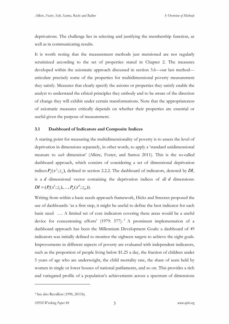
Figure 3.4 First-order stochastic dominance using cumulative distribution functions
Panel I Panel II
The value of a CDF corresponding to certain level of achievement is the proportion of
the population with achievements below that level. Interestingly, if a particular level of
achievement is set as a unidimensional poverty line ( ' Ub z ), then the value of the CDF
at Uz is the headcount ratio 0P (see section 2.1). Thus, � �x UF z and � �y UF z are the
headcount ratios for distributions x and y for poverty line Uz , respectively. Then, x FSD
y if and only if � �0 0; ( ; )�U UP x z P y z . In other words, first-order stochastic dominance is
equivalent to the condition when the headcount ratio in distribution x is either equal to
or lower than that in distribution y for all poverty cut-offs. Equivalently, y has no lower
headcount ratio than x for all poverty cut-offs. Moreover, first-order stochastic
dominance provides results beyond the headcount ratio. As Atkinson (1987) shows, if
one distribution first-order stochastically dominates another distribution, then poverty is
equal or lower in the former distribution for all poverty measures (and any monotonic
transformation of these measures) satisfying population subgroup decomposability and
weak monotonicity. The result, as Atkinson discusses, can be extended to measures that
are not necessarily subgroup decomposable.
Unlike in Panel I, Panel II shows a situation where the CDFs cross each other. For all b
to the left of the crossing, � � ( )!x yF b F b , whereas for all b to the right of the crossing,
� � ( )�x yF b F b . Thus, in this case, no distribution first-order stochastically dominates the
other. When a pair of distributions cannot be ranked by first-order stochastic dominance,
one should look at second- or higher-order stochastic dominance. The second-order
stochastic dominance is equivalent to comparing the area underneath the CDFs for every
achievement level. In this section, our objective is to provide a brief overview of the
dominance approach, and so we mainly focus on the first-order stochastic dominance
and its extension to the multidimensional context. Foster and Shorrocks (1988a,b) show
b ' b '' b
Cum
ulat
ive
Dis
trib
utio
n Fu
nctio
n
yF xF( )yF b"
( )xF b"( )yF b'
( )xF b'
b ' b '' b
Cum
ulat
ive
Dis
trib
utio
n Fu
nctio
n
xF
yF
( )yF b"
( )xF b''
( )xF b'
( )yF b'

Alkire, Foster, Seth, Santos, Roche and Ballon 3: Overview of Methods
OPHI Working Paper 84 www.ophi.org 14
how higher orders of stochastic dominance are linked to poverty dominance for different
poverty measures in the Foster–Greer–Thorbecke (FGT) class (see Box 2.1 for a
numerical example of the FGT measures).12 Atkinson (1987) provides a condition when
poverty measures satisfying certain properties agree with the second-order stochastic
dominance condition.
3.3.2 Poverty Dominance in the Multidimensional Framework
This approach has been extended to the multidimensional context by Duclos, Sahn, and
Younger (2006a) and Bourguignon and Chakravarty (2009). Poverty dominance in the
multidimensional framework is slightly different in that it needs to consider the
identification method as well as the assumed relationship between achievements, namely,
whether they are considered substitutes, complements, or independent. As discussed in
Chapter 2, the identification of those who are multidimensionally poor is not as
straightforward as in the unidimensional framework. In a multidimensional dominance
approach, a poverty frontier based on an overall achievement value of well-being for
each individual is used for identification, and the overall achievement is required to be
non-decreasing in each dimensional achievement. The poverty frontier belongs to the so-
called aggregate achievement approach (section 2.2.2) and it is defined as the different
combinations of the d achievements that provide the same overall achievement as an
aggregate poverty line or subsistence level of well-being. If a person‘s set of d
achievements produces a lower level of well-being than the subsistence level of well-
being, then that person is identified as poor.
The poverty frontier method—like other identification methods such as counting—
encompasses the two extreme criteria for identification, namely, union and intersection,
as well as intermediate cases. The poverty frontier method for identification is presented
in Figure 3.5 using two dimensions. The horizontal axis of the diagram represents
achievements in dimension 1, and the vertical axis denotes achievements in dimension 2.
The deprivation cut-offs of both dimensions are denoted by 1z and 2,z respectively. The
intersection frontier is given by the bold black line, and any person with achievement
combinations to the left of and below this line is identified as poor. Similarly, the union
12 For graphical depictions of higher-order stochastic dominance conditions in terms of different dominance curves, see Ravallion (1994) and Foster et al. (2013).

Alkire, Foster, Seth, Santos, Roche and Ballon 3: Overview of Methods
OPHI Working Paper 84 www.ophi.org 15
frontier is given by the dotted line, and any person with achievement combinations to
the left of or below the dotted is considered poor. Finally, an example of an intermediate
criterion is given by the bold grey line, and any person with an achievement combination
falling below this frontier is identified as poor.
Figure 3.5 Identification using poverty frontiers
Poverty dominance is defined by Duclos, Sahn, and Younger (2006a) in the
multidimensional context as follows. Once a poverty frontier is selected for identifying
the poor, for any two societies with achievement matrices X , �Y , the society with
achievement matrix X poverty dominates the society with achievement matrix Y for
poverty measure P, which we refer to as X PY , if and only if � �; ( ; )dP X z P Y z for all
z�z and � �; ( ; )�P X z P Y z for some z�z .
As in the unidimensional framework, the achievement matrices presented in the previous
paragraph may also be represented using joint CDFs XF and YF , respectively.13 Each
column of an achievement matrix can be represented by a univariate marginal
distribution. In a multidimensional framework, in order to have poverty dominance
between X and ,Y it is not sufficient to check for deprivation dominance in each of the
marginal distributions. It is, in fact, possible to have two different joint CDFs that have
the same set of marginal distributions. For example, while comparing child poverty in
two dimensions between Madagascar and Cameroon, Duclos, Sahn, and Younger
(2006a) found that although statistically significant dominance held for each of the
marginal distributions, dominance did not hold for the joint distribution. Hence,
although it was apparent that deprivation was unambiguously higher in one country
13 See Chapter 2 (section 2.2.3) for a definition of joint CDF in the two-dimension case.
Union
Intermediate
Intersection
z 1
Achievements in Dimension 1
Achi
evem
ents
in D
imen
sion
2
z 2
Alkire, Foster, Seth, Santos, Roche and Ballon 3: Overview of Methods
OPHI Working Paper 84 www.ophi.org 16
when examining both dimensions separately, the same could not be concluded when
looking at two dimensions together. It is thus imperative to consider the joint
distribution or the association between dimensions.
How overall multidimensional poverty is sensitive to association between dimensions
depends on the relation between dimensions as discussed in section 2.5.2. If dimensions
are seen as substitutes, then an increase in association between dimensions, with the
same set of marginal distributions, should not reduce overall poverty. On the contrary, if
dimensions are complements, then an increase in association between dimensions, with
the same set of marginal distributions, should not increase poverty. Duclos, Sahn, and
Younger (2006a) present the stochastic dominance results for two dimensions, assuming
the dimensions are substitutes. Thus, they show under the assumption of substitutability
that if the joint cumulative distribution Y lies above the joint cumulative distribution X
or � �1 2 1 2, ( , )!Y XF b b F b b for all 1b 2 ��b , then X PY for all poverty measures that
satisfy weak monotonicity and subgroup decomposability and use either union,
intersection, or any intermediate poverty frontier method for identification. Note that the
condition � �1 2 1 2, ( , )!Y XF b b F b b for all 1b 2 ��b is an intersection-like condition
because � �1 2,YF b b and � �1 2,XF b b denote the shares of population with achievements less
than 1b in dimension 1 and at the same time achievements less than 2b in dimension 2.
This is analogous to the rectangular area bounded by the black bold lines in Figure 3.5.
Thus, the novelty of this finding is that one should only check the intersection-like
condition. For higher-order stochastic dominance conditions, readers are referred to
Duclos, Sahn, and Younger (2006a).14
Bourguignon and Chakravarty (2009) develop related first-order dominance conditions
for multidimensional poverty measurement in the two-dimension case. Unlike Duclos,
Sahn, and Younger, they use a counting approach for identification. They show that for
poverty measures that satisfy deprivation focus, symmetry, replication invariance,
14 Note that when using a sample rather than the whole population, there is a difference between the mathematical conditions for poverty dominance and the statistical tests that determine when such conditions hold in a statistically significant way. In other words, it is possible to find cases in which although mathematically the dominance condition holds, the difference between the two joint distributions is not statistically significant, thus dominance cannot be concluded. Statistical tests for the dominance conditions in the multidimensional case have been developed by Duclos, Sahn, and Younger (2006a) and Batana and Duclos (2010), among others. Issues of statistical significance in poverty comparisons when using samples should also be considered when implementing other methodologies presented in this chapter. Chapter 8 and Chapter 9 present statistical tools to be used alongside the AF methodology.

Alkire, Foster, Seth, Santos, Roche and Ballon 3: Overview of Methods
OPHI Working Paper 84 www.ophi.org 17
population subgroup decomposability, weak monotonicity, and weak deprivation
rearrangement (substitutes), poverty dominance is required with respect to each marginal
distribution and with respect to the joint distribution in the intersection area (the
rectangular area bounded by solid bold lines in Figure 3.5). This result is consistent with
Duclos, Sahn, and Younger (2006a). Additionally, Bourguignon and Chakravarty (2009)
show that for poverty measures that satisfy the same previously mentioned properties
but also converse weak deprivation rearrangement (complements), poverty dominance is
required with respect to each marginal distribution and with respect to the joint
distribution in the union area (L-shaped area bounded by the dotted lines in Figure 3.5).
For a detailed discussion, see Atkinson (2003).
3.3.3 Applications of the Multidimensional Dominance Approach
The Duclos, Sahn, and Younger (2006a) framework has been applied in several empirical
studies. Batana and Duclos (2010) used the technique with two dimensions to compare
multidimensional poverty across six members of the West African Economic and
Monetary Union: Benin, Burkina Faso, Côte d‘Ivoire, Mali, Niger, and Togo. The
comparison of these six countries involved fifteen pairwise comparisons, and identified a
statistically significant dominance relation for twelve of the pairwise comparisons. Anaka
and Kobus (2012) employed the technique, also using two dimensions, to compare
multidimensional poverty across Polish gminas or municipalities. Labar and Bresson
(2011) used this approach to study the change in multidimensional poverty in China
between 1991 and 2006 and showed that the change in multidimensional poverty was not
unambiguous. Gräb and Grimm (2011) extended this multidimensional dominance
framework to the multi-period context and illustrated their approach using data for
Indonesia and Peru.
Other applications of dominance analysis have also been undertaken recently. For
example, Duclos and Échevin (2011) used a dominance approach to find that welfare in
both Canada and the United States did not unambiguously change in terms of the joint
distribution of income and health. In fact, although dominance in terms of income was
prominent across the entire population, dominance across incomes did not hold across
each health status. Extending the Atkinson and Bourguignon (1982) framework using
four dimensions in the Indian context, Gravel and Mukhopadhyay (2010) found a robust

Alkire, Foster, Seth, Santos, Roche and Ballon 3: Overview of Methods
OPHI Working Paper 84 www.ophi.org 18
reduction in multidimensional poverty between 1987 and 2002. The study used
municipality-level information for three dimensions, not household-level information.
The above studies assume that the dimensions are continuous. In practice, most relevant
indicators are discrete. Duclos, Sahn, and Younger (2006b) extend their multidimensional
robustness approach to situations where one dimension is continuous but the rest of the
dimensions may be discrete (Batana and Duclos 2011). For an alternative approach to
discrete variables extending the Atkinson and Bourguignon (1982) framework, see
Yalonetzky (2009, 2013).
3.3.4 A Critical Evaluation
The strength of the dominance approach is that when poverty dominance holds between
a pair, then the comparison is unambiguous. No alternative specifications can alter the
direction of comparison. Thus, it offers a tool to produce strong empirical assertions
about poverty comparisons—assertions that hold across a range of poverty measures and
in spite of any ‗controversial‘ decisions on parameter values. Even if distributions cross,
and thus it is not possible to have a rank, it is possible to check where the crossing has
taken place and identify limited areas of dominance, which can provide important
information. In addition, the dominance approach takes into account the joint
distribution of achievements when identifying the poor and making poverty
comparisons. The dominance approach has been used with both discrete and continuous
data.
Despite its strengths, this approach has certain limitations that prevent it from being
more widely used for empirical analysis. First, when dominance holds, conclusions about
comparisons can be made, but when there is no dominance, no unambiguous
comparisons can be made. In other words, the dominance approach can only provide a
partial ordering—similar to Lorenz dominance in inequality measurement. Second, even
in situations in which dominance comparisons are empirically possible and generate
ordinal rankings of regions or societies across time, it is not possible to compare the
extent of differences in poverty across two populations in any cardinally meaningful way.
In other words, it is not possible to say how poor a region is compared to another or
how much poverty has fallen or gone up over a certain period of time. The complete
orderings and meaningful cardinal comparisons achieved using other methods, such as
axiomatic measures, can be criticized as imposing arbitrariness or ‗creating artificial

Alkire, Foster, Seth, Santos, Roche and Ballon 3: Overview of Methods
OPHI Working Paper 84 www.ophi.org 19
problems‘ (Sen 1997: 5). However, it must also be recognized that the inability to offer a
complete ranking in certain cases can make this tool of limited use from a policy
perspective.
A third limitation of this approach (although not exclusive to it) is that the dominance
conditions depend on assumptions regarding the relationship between achievements
(either substitutes or complements). In practice, all empirical applications so far have
assumed substitutability between achievements because conditions and their statistical
tests in this case are more fully developed. As Duclos, Sahn, and Younger (2006a) point
out, one of the reasons for not pursuing the case of complementarity further is that it
would drastically limit the scope of robust orderings across alternative poverty frontiers.
Furthermore, the test developed by Duclos, Sahn, and Younger (2006a) is more suitable
for measures that use the aggregate achievement approach (poverty frontier) to
identification than for measures that use a counting approach.
Fourth, although in this section we present the results in terms of population, it may be
empirically challenging to compute dominance using more than two or three dimensions
due to the ‗curse of dimensionality‘—the need for the sample size to increase
exponentially with the number of dimensions. As Duclos, Sahn, and Younger (2006a)
put it, ‗in theory, extending our results to more than two dimensions is straightforward.
In practice, though, most existing datasets in developing countries are probably not large
enough to support tests on more than a few dimensions of wellbeing. This is because the
curse of dimensionality … (p. 944)‘. In such cases of higher dimensionality, other tests or
procedures may be required.15 Another relevant point for the empirical implementation
of the dominance approach is that there is often noise at the extremes of the distribution
that one may wish to ignore, because otherwise results may be artificially biased. For this
reason, one may want to base the dominance criteria on a range that starts, for example,
at certain percent of the median of the distribution of each variable.
Finally, in the multidimensional context, dominance results beyond first order require
more stringent conditions on the individual poverty function, such as on signs of third
order, fourth order, derivatives, and cross derivatives, which are less intuitive (see
Duclos, Sahn, and Younger 2006a and Atkinson 2003).
15 This is well discussed in Anderson (2008), and several empirical routes have been designed due to this problem, as well as the problem of correlated samples. Of course all measures must assess how many indicators are enough (Chs 6, 8).

Alkire, Foster, Seth, Santos, Roche and Ballon 3: Overview of Methods
OPHI Working Paper 84 www.ophi.org 20
The remaining three sections present methodologies that create indices of
multidimensional poverty reflecting the joint distribution across dimensions. As in the
case of Venn diagrams and the dominance approach, each approach requires that
information be available for the same unit of analysis so that the joint distribution among
dimensions can be captured. We first outline some of the widely applied multivariate
statistical techniques used in the analysis and measurement of multidimensional poverty
and well-being.
3.4 Statistical Approaches
Statistical techniques are widely used in the design of poverty measures as well as in
measures of well-being (Nardo et al. 2008; Maggino and Zumbo 2012). Key techniques
include principle component analysis, multiple correspondence analysis, cluster analysis,
latent class analysis, and factor analysis. These techniques use information from the joint
distribution of indicators to inform different aspects of poverty measurement such as
identifying who is poor, setting indicator weights, constructing individual deprivation
scores, and aggregating information into poverty indices representing the level of poverty
in a society. The techniques are often used because they are well-documented and
allegedly less controversial than normative judgements. This section first provides a
synthetic overview of the various contributions of statistical techniques to poverty
measurement design and their applicability to cardinal and ordinal data. It then
introduces the most commonly implemented techniques of principle component
analysis, multiple correspondence analysis, factor analysis, and structural equation
modelling. The section concludes with an assessment of the insights and oversights that
can occur in measures based on statistical approaches.
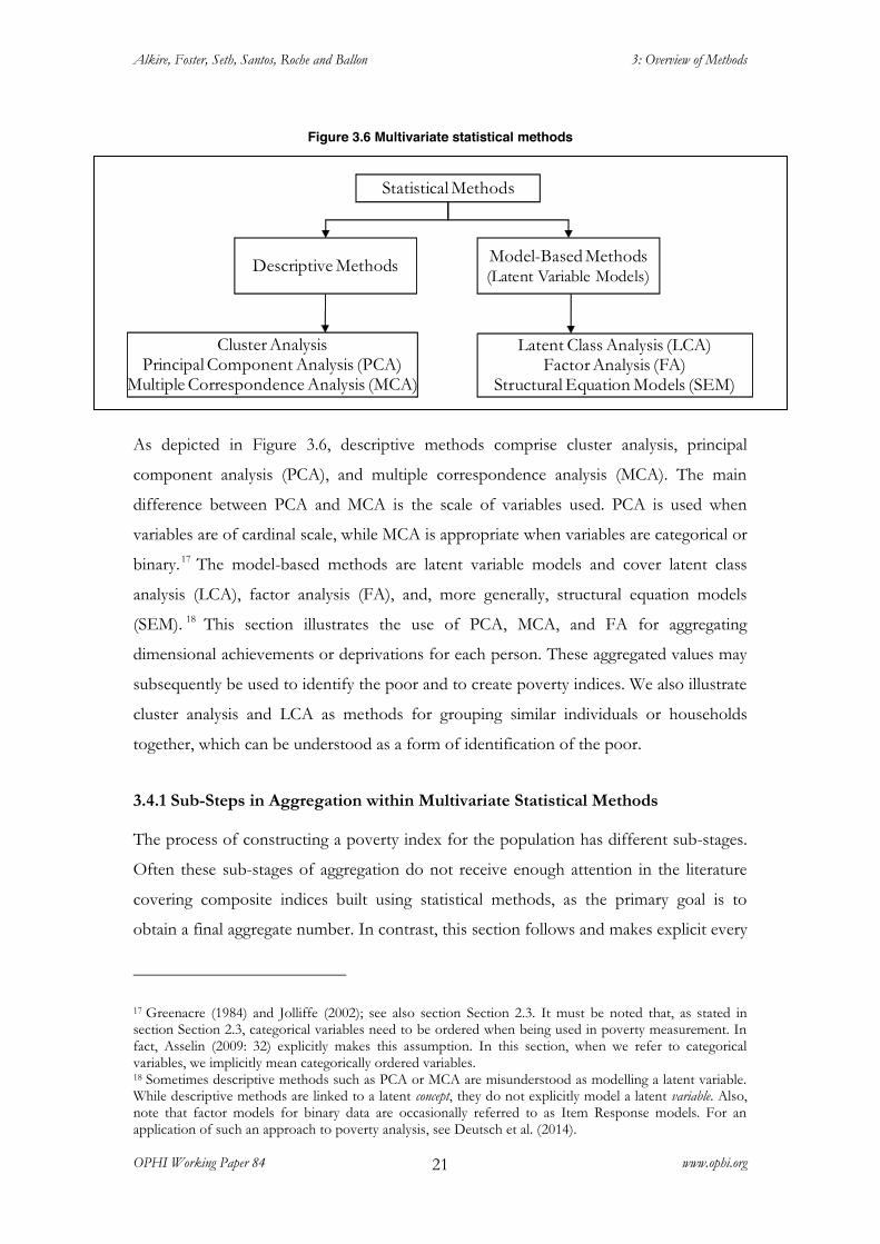
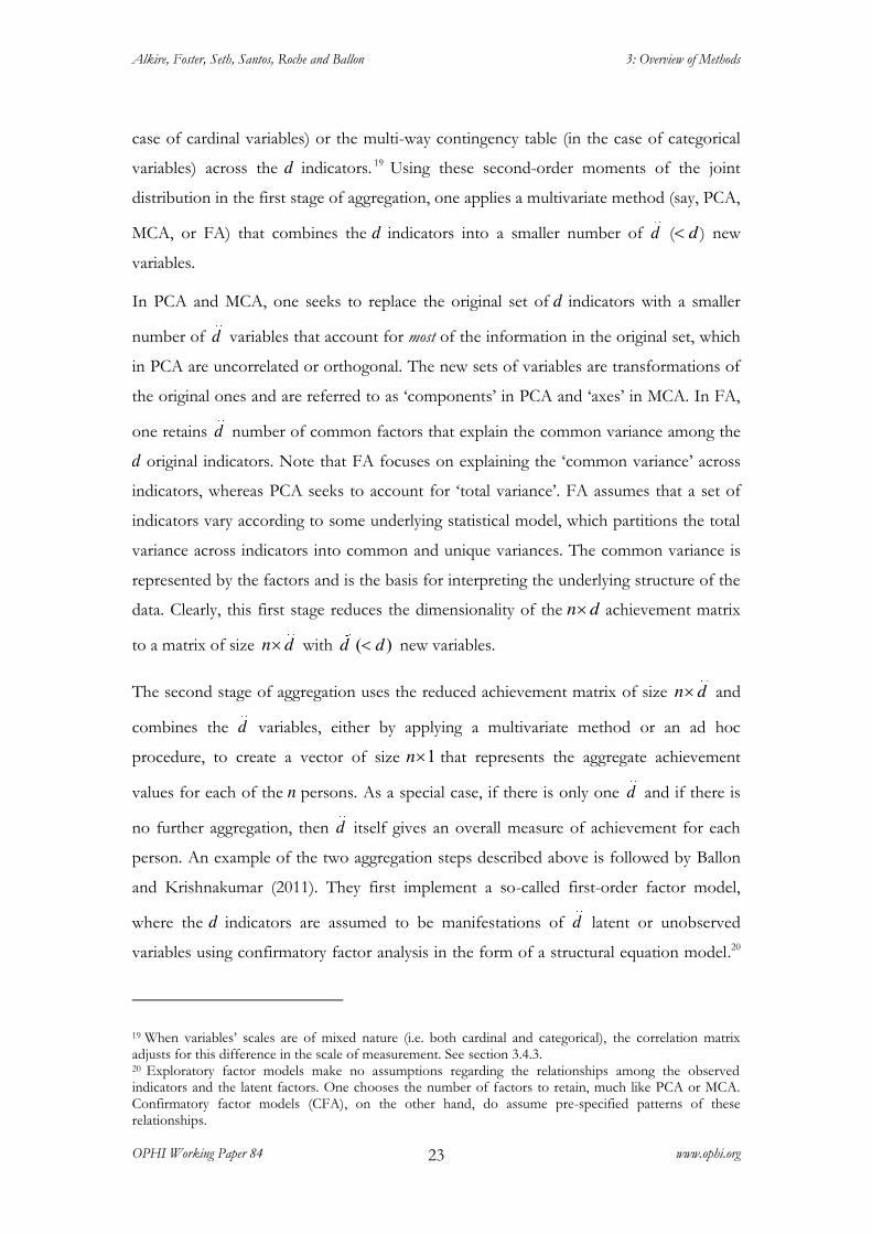
We divide the statistical techniques into two categories. Figure 3.6 sketches this
classification. The two categories are: descriptive methods, whose primary aim is to
describe a multivariate dataset, and model-based methods, which additionally attempt
to make inferences about the population (Bartholomew et al. 2008). One of the
challenges in surveying statistical approaches is that applied methodologies vary widely,
but our classification does summarize the methods most frequently used.16
16 For discussions and applications of further statistical methods, see Mardia, Kent, and Biby (1979) and Bartholomew et al. (2008); for poverty in particular, see Kakwani and Silber (2008).
Alkire, Foster, Seth, Santos, Roche and Ballon 3: Overview of Methods
OPHI Working Paper 84 www.ophi.org 21
Figure 3.6 Multivariate statistical methods
As depicted in Figure 3.6, descriptive methods comprise cluster analysis, principal
component analysis (PCA), and multiple correspondence analysis (MCA). The main
difference between PCA and MCA is the scale of variables used. PCA is used when
variables are of cardinal scale, while MCA is appropriate when variables are categorical or
binary.17 The model-based methods are latent variable models and cover latent class
analysis (LCA), factor analysis (FA), and, more generally, structural equation models
(SEM). 18 This section illustrates the use of PCA, MCA, and FA for aggregating
dimensional achievements or deprivations for each person. These aggregated values may
subsequently be used to identify the poor and to create poverty indices. We also illustrate
cluster analysis and LCA as methods for grouping similar individuals or households
together, which can be understood as a form of identification of the poor.
3.4.1 Sub-Steps in Aggregation within Multivariate Statistical Methods
The process of constructing a poverty index for the population has different sub-stages.
Often these sub-stages of aggregation do not receive enough attention in the literature
covering composite indices built using statistical methods, as the primary goal is to
obtain a final aggregate number. In contrast, this section follows and makes explicit every
17 Greenacre (1984) and Jolliffe (2002); see also section Section 2.3. It must be noted that, as stated in section Section 2.3, categorical variables need to be ordered when being used in poverty measurement. In fact, Asselin (2009: 32) explicitly makes this assumption. In this section, when we refer to categorical variables, we implicitly mean categorically ordered variables. 18 Sometimes descriptive methods such as PCA or MCA are misunderstood as modelling a latent variable. While descriptive methods are linked to a latent concept, they do not explicitly model a latent variable. Also, note that factor models for binary data are occasionally referred to as Item Response models. For an application of such an approach to poverty analysis, see Deutsch et al. (2014).
Descriptive Methods Model-Based Methods(Latent Variable Models)
Cluster AnalysisPrincipal Component Analysis (PCA)
Multiple Correspondence Analysis (MCA)
Latent Class Analysis (LCA)Factor Analysis (FA)
Structural Equation Models (SEM)
Statistical Methods
Alkire, Foster, Seth, Santos, Roche and Ballon 3: Overview of Methods
OPHI Working Paper 84 www.ophi.org 22
single step followed in each of these techniques and itemizes the decisions made at each
step. For different decisions taken, at each stage, different conclusions may arise. This
novel presentation will enable readers to transparently compare poverty measures built
using statistical methods with other approaches such as counting-based methods.
For example, when PCA or MCA is used, one needs to determine the number of
components or axes to retain. There are several rules for choosing among these ‗new‘
variables, which are essentially transformations of the original indicator variables. The
users of PCA or MCA are often unaware of these various rules and their consequences in
the construction of the individual achievement/deprivation values or the final poverty
index (Coste et al. 2005). Moreover, if more than one component or axis is retained, the
user also needs to decide how to combine them. In this regard, Asselin (2009) discusses
the consistency requirements (axioms) that, in his view, a multidimensional poverty index
obtained through MCA should satisfy and suggests using more than the first factorial
axis. Whether or not one agrees with these particular axioms and requirements, it shows
that when constructing measures through multivariate techniques one needs to be aware
of the intermediate processes of aggregation, as the decisions made at each stage are
likely to lead to varying results.
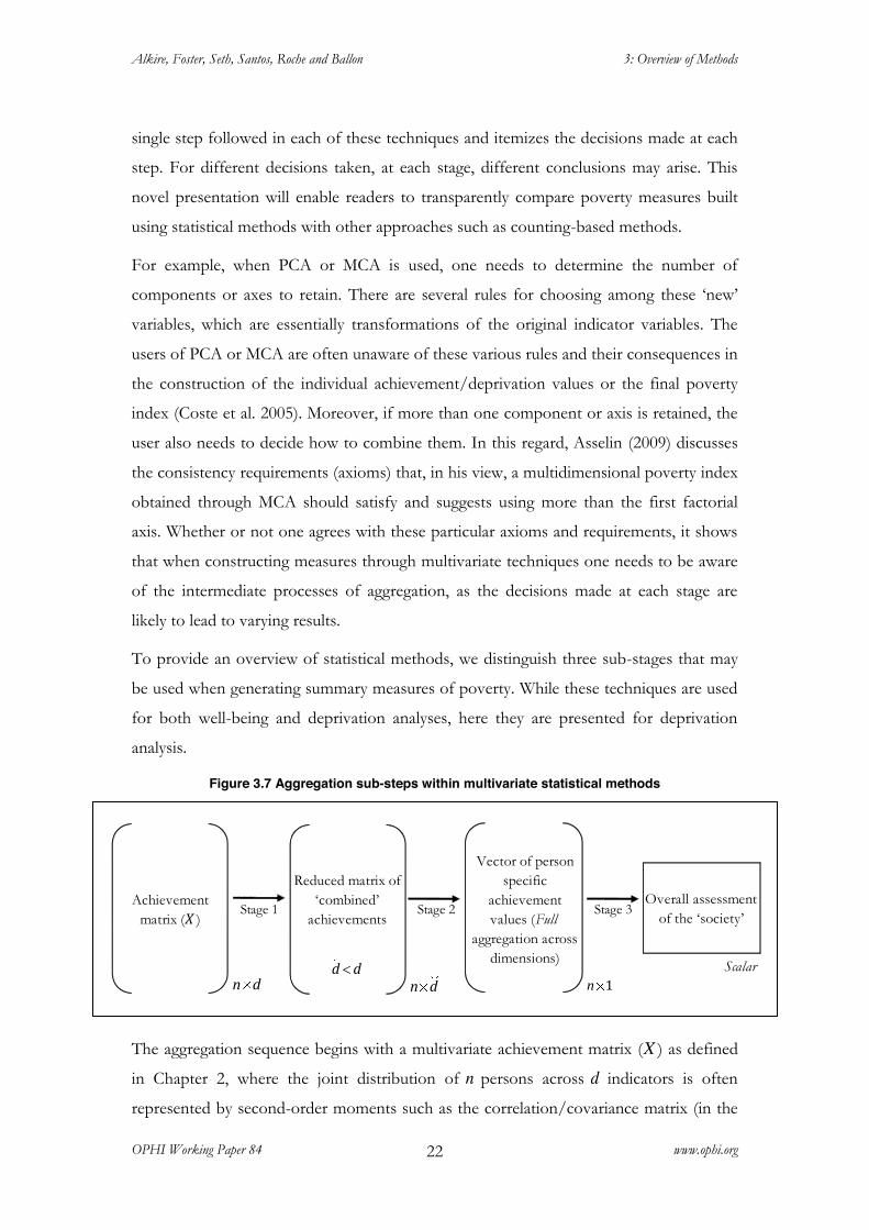
To provide an overview of statistical methods, we distinguish three sub-stages that may
be used when generating summary measures of poverty. While these techniques are used
for both well-being and deprivation analyses, here they are presented for deprivation
analysis.
Figure 3.7 Aggregation sub-steps within multivariate statistical methods
The aggregation sequence begins with a multivariate achievement matrix (X ) as defined
in Chapter 2, where the joint distribution of n persons across d indicators is often
represented by second-order moments such as the correlation/covariance matrix (in the
Stage 1 Stage 2 Stage 3
Scalar
Achievement matrix (X )
Vector of person specific
achievement values (Full
aggregation across dimensions)
Overall assessment of the ‗society‘
Reduced matrix of ‗combined‘
achievements
�d dn dn d 1n
Alkire, Foster, Seth, Santos, Roche and Ballon 3: Overview of Methods
OPHI Working Paper 84 www.ophi.org 23
case of cardinal variables) or the multi-way contingency table (in the case of categorical
variables) across the d indicators. 19 Using these second-order moments of the joint
distribution in the first stage of aggregation, one applies a multivariate method (say, PCA,
MCA, or FA) that combines the d indicators into a smaller number of d (� d ) new
variables.
In PCA and MCA, one seeks to replace the original set of d indicators with a smaller
number of d variables that account for most of the information in the original set, which
in PCA are uncorrelated or orthogonal. The new sets of variables are transformations of
the original ones and are referred to as ‗components‘ in PCA and ‗axes‘ in MCA. In FA,
one retains d number of common factors that explain the common variance among the
d original indicators. Note that FA focuses on explaining the ‗common variance‘ across
indicators, whereas PCA seeks to account for ‗total variance‘. FA assumes that a set of
indicators vary according to some underlying statistical model, which partitions the total
variance across indicators into common and unique variances. The common variance is
represented by the factors and is the basis for interpreting the underlying structure of the
data. Clearly, this first stage reduces the dimensionality of the un d achievement matrix
to a matrix of size n du with ( )d d� new variables.
The second stage of aggregation uses the reduced achievement matrix of size n du and
combines the d variables, either by applying a multivariate method or an ad hoc
procedure, to create a vector of size 1un that represents the aggregate achievement
values for each of the n persons. As a special case, if there is only one d and if there is
no further aggregation, then d itself gives an overall measure of achievement for each
person. An example of the two aggregation steps described above is followed by Ballon
and Krishnakumar (2011). They first implement a so-called first-order factor model,
where the d indicators are assumed to be manifestations of d latent or unobserved
variables using confirmatory factor analysis in the form of a structural equation model.20
19 When variables‘ scales are of mixed nature (i.e. both cardinal and categorical), the correlation matrix adjusts for this difference in the scale of measurement. See section 3.4.3. 20 Exploratory factor models make no assumptions regarding the relationships among the observed indicators and the latent factors. One chooses the number of factors to retain, much like PCA or MCA. Confirmatory factor models (CFA), on the other hand, do assume pre-specified patterns of these relationships.

Alkire, Foster, Seth, Santos, Roche and Ballon 3: Overview of Methods
OPHI Working Paper 84 www.ophi.org 24
Then, they suggest using a so-called second-order factor model that combines these d
variables into an ‗overall‘ factor, assuming that these d variables are also manifestations
of a latent variable.21 The overall factor score for each person in this case is analogous to
the aggregate achievement value in the aggregate achievement approach to identification
described in section 2.2.2.
Alternatively, rather than using a multivariate method, one may use an ad hoc
procedure—a common one being to combine the d variables using some form of
weighted average. For example, in their study of quality of life among forty-three
countries, Rahman et al. (2011) use the proportion of the total variance accounted for
each component as its weight. Krishnakumar and Ballon (2008), in their estimation of
children‘s capabilities in Bolivia, use the inverse of the component‘s variance as its
weight. Note that the choice of weights may affect the results.
The third stage aggregates the person-specific aggregate achievement values of all
persons into an index that reflects the overall poverty of the population. Clearly, to
achieve such a poverty index, identification of the poor needs to take place, comparing
the person-specific aggregate achievement value against some poverty cut-off. This cut-
off may be absolute but typically is relative in these methods. Thus, in this third stage,
the 1un vector, containing person-specific achievements, is compressed into a scalar
measure to assess the society. Section 3.4.2 presents a brief overview of implementations
of the various statistical approaches.
3.4.2 Applications of Statistical Approaches in Poverty Aggregation
Filmer and Pritchett (1999, 2001) applied PCA to a set of asset variables found in the
Demographic and Health Surveys and retained the first principal component in order to
construct a household asset index. The asset index scores were standardized in relation
to a standard normal distribution with a mean of 0 and a standard deviation of 1. All
individuals in each household were assigned the household‘s standardized asset index
21 Second-order factor models are applied when the hypothesis is that several related factors can be accounted for by one or more common underlying higher-order factors. In multidimensional poverty, a first-order model hypothesizes that each dimension is a factor measured by multiple indicators. As each of these dimensions is a partial representation of the multidimensional phenomenon of poverty, one can further hypothesize that each dimension can be accounted for by a single and common factor (see Ballon and Krishnakumar 2011).

Alkire, Foster, Seth, Santos, Roche and Ballon 3: Overview of Methods
OPHI Working Paper 84 www.ophi.org 25
score, and all individuals in the sample population were ranked according to that score.
The sample population was then divided into quintiles of individuals, with all individuals
in a single household being assigned to the same quintile. In this case, the third sub-step
was not completed and no scalar societal measure was generated. Filmer and Prichett‘s
approach has since been used for the analysis of health inequalities (Bollen et al. 2002;
Gwatkin et al. 2000; Schellenberg et al. 2003), child nutrition (Sahn and Stifel 2003), and
child mortality (Fay et al. 2005; Sastry 2004) among other purposes. In the field of
poverty and inequality, PCA and FA have been applied by Sahn and Stifel (2000), Stifel
and Christiaensen (2007), McKenzie (2005), Lelli (2001), and Roche (2008) among
others.
Within the correspondence analysis literature, we find applications by Asselin and Anh
(2008), Booysen et al. (2008), Deutsch, Silber, and Verme (2012), Batana and Duclos
(2010), and Ballon and Duclos (2014). Asselin and Anh (2008) built a MCA composite
index of human and physical assets to study poverty dynamics in Vietnam between 1999
and 2002. Booysen et al. (2008) applied MCA to obtain an asset index for comparing
poverty over time and across seven West African countries. Deutsch, Silber, and Verme
(2012) use correspondence analysis to analyse social exclusion in Macedonia. Batana and
Duclos (2010) calculated a multidimensional index of wealth (ownership of durable
goods and access to services) using MCA for a series of sub-Saharan African countries.
This index was used to compare cross-country multidimensional poverty via sequential
stochastic dominance analysis. Ballon and Duclos (2014) applied MCA to obtain two sets
of values reflecting households‘ access to ‗public‘ assets (basic services) and ‗private‘
assets (durable goods) in North and South Sudan. These two sets of MCA values were
further used for measuring multidimensional poverty according to the Alkire and Foster
(2011a) methodology.
Interesting applications of statistical techniques up to the last stage of aggregation (i.e.
obtaining an overall well-being or deprivation index for the society) include those used
by Kuklys (2005), Klasen (2000), and Ballon and Krishnakumar (2011). Kuklys used the
factor scores obtained from a structural equation model as the input distributions in
FGT poverty-type measures (Foster, Greer, and Thorbecke 1984). Ballon and
Krishnakumar (2011) proposed an index of capability deprivation, where the input
variables were the factor scores of a structural equation model that estimated children‘s
capabilities. Klasen (2000) derived a material deprivation index for households in South

Alkire, Foster, Seth, Santos, Roche and Ballon 3: Overview of Methods
OPHI Working Paper 84 www.ophi.org 26
Africa. Other interesting applications of structural equation models in development
studies, although not focused on aggregation into a scalar measure, are the ones
proposed by Di Tommaso (2007) for India, Wagle (2009) for Nepal and the United
States, and Ballon (2011) for Cambodia.
3.4.3 A Brief and Formal Outline of Different Statistical Approaches
This section presents in greater detail the three methods most commonly implemented
for both identification and aggregation, namely, PCA, MCA, and FA. Additional
methodological variations are also implemented; this section covers the more standard
approaches.
3.4.3.1 Principal Component Analysis
Principal component analysis was first proposed by Pearson (1901) and was further
developed by Hotelling (1933). Hotelling derived principal components using
mathematical arguments, leading to the standard algebraic derivation that optimizes the
variance of the original dataset (known as an ‗eigen decomposition‘), while Pearson
approached PCA geometrically.22
The main aim of PCA is parsimony.23 Basically, in PCA the d indicator variables are
transformed into linear combinations called principal components. In this search for
parsimony, one seeks to find fewer principal components (PCs) that retain most of the
information in the original set of observed indicators. The information retained by the
PCs is measured by the proportion of the total (sample) variance that is accounted for in
each of the PCs. There is usually a trade-off between a gain in parsimony and a loss of
information. If the original indicators are correlated, and especially if they are highly
correlated, then one can replace them by a relatively small set of PCs—say, d , where d
is smaller than d . If the original indicators are only slightly correlated, the resulting PCs
22 Pearson‘s geometric derivation defines principal components as ‗optimal‘ lines and planes. The first
principal component is the line that best fits a set of n points in a reduced d dimensional space. The first
two principal components define a plane that best fits a cloud of n points in the d dimensional space, and likewise for other principal components. Jolliffe (2002) and Basilevsky (1994) provide historical surveys of the development of PCA. 23 Other aims of PCA include addressing multicollinearity issues in regression analysis, the detection of outliers, or the interpretation of the underlying structure of a set of observed indicators (Jolliffe 2002). The latter is similar to factor analysis, which is discussed later on in this section, but there are important differences between these two techniques.
Alkire, Foster, Seth, Santos, Roche and Ballon 3: Overview of Methods
OPHI Working Paper 84 www.ophi.org 27
will largely reflect the original set without much gain in parsimony. Clearly, the full set of
PCs will fully account for the total variance of the original indicators and will be the case
where no reduction in dimensionality is achieved. A particular feature of the PCs is that
these are uncorrelated (orthogonal).
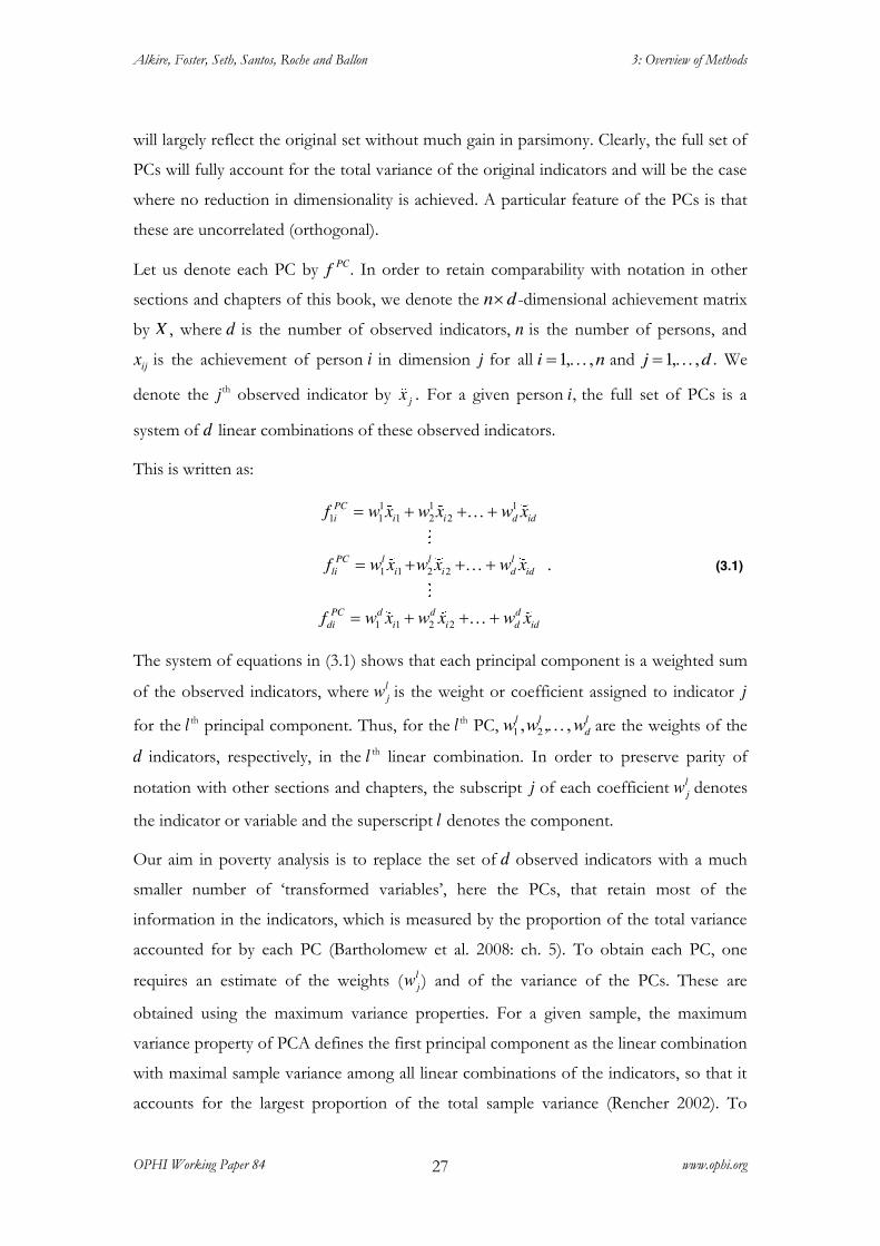
Let us denote each PC by PCf . In order to retain comparability with notation in other
sections and chapters of this book, we denote the un d -dimensional achievement matrix
by X , where d is the number of observed indicators, n is the number of persons, and
ijx is the achievement of person i in dimension j for all 1, , }i n and 1, , }j d . We
denote the j th observed indicator by jx . For a given person ,i the full set of PCs is a
system of d linear combinations of these observed indicators.
This is written as:
1 1 11 1 1 2 2
1 1 2 2
1 1 2 2
.
PCi i i d id
PC l l lli i i d id
PC d d ddi i i d id
x x x
x x x
x x x
f w w w
f w w w
f w w w
� �}�
� �}�
� �}�
(3.1)
The system of equations in (3.1) shows that each principal component is a weighted sum
of the observed indicators, where ljw is the weight or coefficient assigned to indicator j
for the l th principal component. Thus, for the l th PC, 1 2, , ,}l l ldw w w are the weights of the
d indicators, respectively, in the l th linear combination. In order to preserve parity of
notation with other sections and chapters, the subscript j of each coefficient ljw denotes
the indicator or variable and the superscript l denotes the component.
Our aim in poverty analysis is to replace the set of d observed indicators with a much
smaller number of ‗transformed variables‘, here the PCs, that retain most of the
information in the indicators, which is measured by the proportion of the total variance
accounted for by each PC (Bartholomew et al. 2008: ch. 5). To obtain each PC, one
requires an estimate of the weights ( ljw ) and of the variance of the PCs. These are
obtained using the maximum variance properties. For a given sample, the maximum
variance property of PCA defines the first principal component as the linear combination
with maximal sample variance among all linear combinations of the indicators, so that it
accounts for the largest proportion of the total sample variance (Rencher 2002). To

Alkire, Foster, Seth, Santos, Roche and Ballon 3: Overview of Methods
OPHI Working Paper 84 www.ophi.org 28
achieve a maximum, one needs to add some normalization constraints on the coefficients ljw , which usually require that the sum of squares of these coefficients is equal to one.24
This leads to an optimization problem, where one maximizes the variance of the first
linear combination subject to the sum of squares of the weights being equal to one to
find the coefficients 1jw for all 1,.. j d, and the variance of the first PC. If we write the
first principal component 1( )PCf as
1
11
,d
PCj j
j
xf w
¦ (3.2)
its sample variance
� � ' '
'
21 1 2 1 11
1 1
d d dPC
j j j j j j jjj j j j
Var f Var w w s w sx w z
ª ºª º �« »¬ ¼
¬ ¼¦ ¦ ¦ (3.3)
is given by the variance of the linear combination of the indicators, which takes into
account the sample variances 2js of the indicators and also the sample covariances 'jj
s
across indicators. Thus to obtain the first PC, one will maximize 1ª º¬ ¼PCVar f given by
equation (3.3) subject to � �21
1
1
¦d
jj
w . This will provide an estimate of the weight vector
1jw for all 1,.., j d and of the variance of 1
PCf .
The second principal component is the linear combination that accounts for the second
largest proportion of total variance among indicators that is orthogonal (uncorrelated) to
the first PC. To find the second PC one will maximize 2ª º¬ ¼PCVar f subject to � �22
1
1
¦d
jj
w
and the orthogonality constraint between the first and second PC, given by 1 2
1
0
¦d
j jj
w w .
This optimization will give estimates of the weight vector 2jw for all 1, , }j d and of the
variance of 2PCf . In a similar manner, one can define the third PC as the weight vector
that maximizes the third linear combination, given that the sum of squares of the
coefficients is equal to one and that the third PC is orthogonal to the first two PCs, and
so on and so forth for the fourth PC, fifth, and d th PC.
24 This restriction ensures that weights are non-negative and each weight is bounded above by one.

Alkire, Foster, Seth, Santos, Roche and Ballon 3: Overview of Methods
OPHI Working Paper 84 www.ophi.org 29
It turns out that the maximization problem is equivalent to finding the eigenvalues and
eigenvectors of the sample covariance matrix. 25 The eigenvalues usually denoted by
1 2, , ,} dO O O are listed from largest to smallest 1 2t }t dO O O and determine the variances
of each PC. The eigenvector associated with each eigenvalue determines the weights or
coefficients of the indicators on the corresponding component. Thus the variance of
component l , ª º¬ ¼PC
lVar f , is the eigenvalue ,lO and the eigenvector 1 2( , , , ) }l l l ldw w ww
associated with this eigenvalue lO gives the coefficients or weights of each indicator on
the l th PC. The percentage of variance accounted for by PClf is therefore
1 2/ ( )� �}�l dO O O O .
When the units of measurements across (cardinal) indicators vary or when the variances26
across them differ widely, one may wish to use the sample correlation matrix R instead
of the sample covariance matrix S. This is equivalent to standardizing each of the d
indicators to have a mean of 0 and variance of 1, then finding the PCs of the
standardized covariance matrix R. The principal components obtained from R will
contribute evenly to total variation and thus be more interpretable. However, the
components extracted from S, the unstandardized covariance matrix, will differ from
those extracted from the correlation matrix 27 R, and so the percentage of variance
accounted for by the components of each of the matrices will be different. Thus the
decision to use either R or S may affect the final results.
Once one has computed the PCs and obtained an estimate of the weights and the
variances of each PC, one needs to decide the number of components to retain. This is
especially important in studies of deprivation that use PCA as the basis for obtaining
either a person-specific or a society measure of poverty, as the results may vary
depending on number of PCs retained. This aspect has been thoroughly examined by
Coste et al. (2005) while obtaining synthetic measures of deprivation in health.
There is a multiplicity of rules for determining the number of components to retain
(Jolliffe 2002). The main guidelines for selecting components in PCA are based on a
25 For definitions of eigenvalues, eigenvectors, and singular value decomposition, see the statistical Appendix A.6 of Mardia, Kent, and Bibby (1979). 26 In PCA, by meaningful variances, we mean the variances of cardinal indicators having a meaningful scale of measurement. For binary or categorical indicators, MCA should be used instead of PCA. 27 Note that for R the sum of the eigenvalues will be equal to the number of indicators, d in our context,
and hence the proportion of variance due to the l th PC is /l dO , where lO is the l th eigenvalue of R.
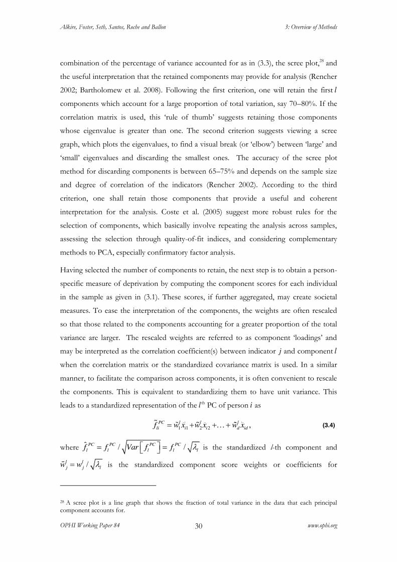
Alkire, Foster, Seth, Santos, Roche and Ballon 3: Overview of Methods
OPHI Working Paper 84 www.ophi.org 30
combination of the percentage of variance accounted for as in (3.3), the scree plot,28 and
the useful interpretation that the retained components may provide for analysis (Rencher
2002; Bartholomew et al. 2008). Following the first criterion, one will retain the first l components which account for a large proportion of total variation, say 70–80%. If the
correlation matrix is used, this ‗rule of thumb‘ suggests retaining those components
whose eigenvalue is greater than one. The second criterion suggests viewing a scree
graph, which plots the eigenvalues, to find a visual break (or ‗elbow‘) between ‗large‘ and
‗small‘ eigenvalues and discarding the smallest ones. The accuracy of the scree plot
method for discarding components is between 65–75% and depends on the sample size
and degree of correlation of the indicators (Rencher 2002). According to the third
criterion, one shall retain those components that provide a useful and coherent
interpretation for the analysis. Coste et al. (2005) suggest more robust rules for the
selection of components, which basically involve repeating the analysis across samples,
assessing the selection through quality-of-fit indices, and considering complementary
methods to PCA, especially confirmatory factor analysis.
Having selected the number of components to retain, the next step is to obtain a person-
specific measure of deprivation by computing the component scores for each individual
in the sample as given in (3.1). These scores, if further aggregated, may create societal
measures. To ease the interpretation of the components, the weights are often rescaled
so that those related to the components accounting for a greater proportion of the total
variance are larger. The rescaled weights are referred to as component ‗loadings‘ and
may be interpreted as the correlation coefficient(s) between indicator j and component l when the correlation matrix or the standardized covariance matrix is used. In a similar
manner, to facilitate the comparison across components, it is often convenient to rescale
the components. This is equivalent to standardizing them to have unit variance. This
leads to a standardized representation of the l th PC of person i as
1 1 2 2 ,PC l l lli i i d idxw w x xf w � �}� (3.4)
where / /ª º ¬ ¼PC PC PC PC
l l l l lf f Var f f O is the standardized l-th component and
/ l lj j lw w O is the standardized component score weights or coefficients for
28 A scree plot is a line graph that shows the fraction of total variance in the data that each principal component accounts for.

Alkire, Foster, Seth, Santos, Roche and Ballon 3: Overview of Methods
OPHI Working Paper 84 www.ophi.org 31
component l and indicator j, for all l and all j . Note that the number of retained factors
and the choice of weight and standardization procedures may affect results.
As in section 3.4.2, the dimensional components may be combined into an individual
score using a multivariate or an ad hoc procedure, and individual scores may be
aggregated, for example, by using a simple average.
3.4.3.2 Multiple Correspondence Analysis
When the indicators are ordinal, binary, or categorical, a more suitable multivariate
technique for a lower-dimensional description of the data is correspondence analysis
(CA). The use of correspondence analysis in social sciences increased significantly in the
late 1980s, inspired mainly by the work of Bourdieu (1986, 1987). The history of CA can
be traced back to the mid 1930s during which various authors defined correspondence
analysis in different but mathematically equivalent ways.29 An intuitive and widely used
definition in the multivariate statistical literature is the geometrical approach suggested in
Greenacre (1984) and Greenacre and Blasius (2006) who follow the ideas of the French
mathematician and linguist Jean-Paul Benzécri (Benzécri and Bellier 1973). This
geometric approach sees CA as an adaptation of PCA to categorical data.
Like PCA, CA is based on a geometric decomposition.30 Simple correspondence analysis
explores the association between two categorical indicators, lx and ' l
x using a two-way
contingency table or cross-tab of relative frequencies denoted by P, which is also referred
to as the correspondence matrix. The elements of P are the set of relative frequencies
across pairs of categories of the two indicators, denoted by 𝕡𝑙𝑙′ , for all ' '1, , ; 1,l l } } , where and 'denote the number of response categories of each
of the two indicators, respectively.
The basic MCA algorithm analyses the association using the singular value
decomposition (SVD) of the matrix of standardized residuals Z with the 'll th element
being 𝕫𝑙𝑙′ = 𝕡𝑙𝑙′ − 𝕡𝑙+ 𝕡+𝑙′ / 𝕡𝑙+ 𝕡+𝑙 , where 𝕡𝑙+ = 𝕡𝑙𝑙′𝕃𝑙=1 and 𝕡+𝑙′ =
29 Greenacre (1984) and Gifi (1990) provide an overview of the historical development of CA dating back to Hirschfeld (1935), Fisher (1940), and Guttman (1941). Louis Guttman was the first to extend the ideas behind simple CA to the general case of more than two variables, leading to what today is known as MCA. 30 In PCA this involves the eigen decomposition of the correlation matrix, while in CA this involves the singular value decomposition of the standardized residual matrix.

Alkire, Foster, Seth, Santos, Roche and Ballon 3: Overview of Methods
OPHI Working Paper 84 www.ophi.org 32
𝕡𝑙𝑙′𝕃′𝑙′ =1 are the row and column margins. These margins are the marginal frequencies
also known as masses in the CA literature (see section 2.2.3 for an explanation of a 2 2u
contingency table). The standardized residuals 𝕫𝑙𝑙′ are similar to those used in the
calculation of the Pearson chi-square statistic ( 2F ), which measures dissimilarity between
the row and column profiles of a two-way contingency table. For this reason, in CA the
total variance in the cross-tab, called ‗total inertia‘, is equal to 2F divided by the sample
size. Similar to PCA, in CA one also needs estimates of the total inertia (‗variance‘) and
of the component weights or coefficients to obtain person-specific achievement values.
These are obtained from the SVD of Z where the eigenvalues, 31 called ‗principal
inertias‘, quantify the variance in the cross-tab and the singular vectors give the axes‘
coordinates for the low-dimensional representation and play a similar role as weights or
coefficients in PCA. When the reduction in dimensionality involves two axes, one can
plot the axes‘ coordinates, providing a visual representation (bi-plot) of the association
across categories of the indicators.
In the general case of a set of categorical indicators, CA extends the analysis to a
multiway table of all associations amongst pairs of variables. This is an MCA, which
performs a CA on a Burt or indicator matrix. The indicator matrix I is an individuals-by-
categories matrix. The elements of this matrix are 0s and 1s with columns for all
categories of all indicators and rows corresponding to individuals. A value of 1 indicates
that a category is observed; a 0 indicates that it is not. The Burt matrix is a matrix of all
two-way cross-tabulations of the categorical variables. MCA on either the Burt or
indicator matrix gives equivalent standard coordinates, but the total principal inertias
obtained from each of the two approaches differ.
As with simple correspondence analysis, the principal inertias and the singular vectors are
used to obtain person-specific achievement or deprivation values. Thus, the person‘s
deprivation score will vary depending on whether the Burt or indicator matrix is used.
The Burt matrix is the most commonly used.32
31 Or squared singular values. 32 A slight inconvenience of MCA is that it artificially inflates the chi-squared distances between profiles and the total inertia. This can be partially remedied after CA of the Burt matrix by scale readjustments of the MCA solution. Additionally, in MCA the notion of accounted inertia has less justification because the
2F statistic involves distances not only between categories of two different variables but also between two categories of the same variable. These within-variable distances depend only on the marginal frequencies of

Alkire, Foster, Seth, Santos, Roche and Ballon 3: Overview of Methods
OPHI Working Paper 84 www.ophi.org 33
3.4.3.3 Factor Analysis and Structural Equation Modelling
Factor Analysis (FA) and structural equation models fit within the broad class of Latent
Variable Models (LVM). LVMs are regression models that make assumptions and
express relationships between observed and unobserved (or latent) variables. The
development of the single-factor model was initiated by Spearman (1904) to measure
overall intelligence. This was further generalized by Garnett (1919) and Thurstone
(1931), among others. In an FA model, the main assumption is that several observed
indicators depend on the same latent variable or variables. This dependence is reflected
in the correlation matrix across indicators. Thus FA is a model-based technique that
assumes an underlying statistical model regarding the variation in a set of indicators. As
discussed earlier, the common variance is represented by a factor. Like PCA, FA is also
used as a data reduction method; however, there is a fundamental difference between the
two methods. PCA is a descriptive method that attempts to interpret the underlying
(latent) structure of a set of indicators on the basis of their total variation, while FA is a
model-based method that focuses on explaining the common variance across indicators
instead of total variance.
Factor models could be either exploratory or confirmatory. Exploratory factor analysis
(EFA) models make no prior assumptions regarding the pattern of relationships among
the observed indicators and the latent factors. Confirmatory factor analysis (CFA)
models do assume a pre-specified pattern of relationships.
In the general linear (exploratory) factor model with observed cardinal indicators, the d
indicators are expressed as linear combinations of a few unobserved factors
ˇ1 2, , , ( )FA FA FA
df f f d d} � . For a given individual i , this takes the form of a
measurement equation:
1 20 1 2 ; 1, ,FA FA d FA
ij j i j i j ijdif f f jx dJ J J J � � �}� � } , (3.5)
where 1 2, , , FA FA FAdf f f} are the common factors, ij are residuals, and l
jJ is the l th
regression parameter for the j th indicator—referred to as ‗factor loading‘.
each indicator and do not contribute to the analysis of association with other indicators (cf. Greenacre and Blasius 2006).

Alkire, Foster, Seth, Santos, Roche and Ballon 3: Overview of Methods
OPHI Working Paper 84 www.ophi.org 34
The general linear factor model assumes that the factors have a mean of 0, a variance of
1, and are uncorrelated with each other. It also assumes that the residuals have a mean of
0, are heteroscedastic, and that they are uncorrelated with the factors. The general linear
factor model may lead to the normal linear factor model if, additionally, it is assumed
that the observed indicators and the residuals follow a multivariate normal distribution.
The essence of factor models is the correlation structure of the model‘s indicators. This
is reflected by the correlation matrix predicted by the model. To fit factor models, one
looks for values of the parameters such that the observed correlation matrix is as close as
possible to the one predicted by the model. The estimation could be done through a
variety of methods comprising generalized least squares and maximum likelihood (cf.
Joreskog 1970; Bollen 1989; Joreskog and Sorbom 1999; Muthén 1984; Muthén and
Muthén 1998–2012). The adequacy of the model and the selection of the number of
factors to retain are checked through goodness-of-fit statistics (Bartholomew and
Tzamourani 1999). When the observed indicators comprise categorical variables it is
possible to construct a meaningful correlation matrix. This ‗adjusted‘ correlation matrix
will include standard Pearson correlations for pairs of cardinal indicators, tetrachoric
(polychoric) correlations for pairs of binary (categorical) indicators, and bi-serial
(polyserial) correlations for pairs of cardinal and dichotomous (categorical) variables. For
such purposes, one can assume that a latent continuous variable, normally distributed,
underlies every categorical variable. This is referred to as the underlying variable
approach (cf. Joreskog and Moustaki 2001).
Following the estimation, and to ease interpretation, the factors are transformed into a
‗new‘ set of factors. This process is called ‗rotation‘ and involves orthogonal and oblique
rotations, among others. The latter requires relaxing the assumption of absence of
correlation among factors.
Once the factors have a meaningful interpretation, it is possible to obtain person-specific
achievement values on the latent variable. The prediction of the
achievement/deprivation values could be achieved through several methods that lead to
highly correlated but different cardinal values of the factor (Bollen 1989). In the presence
of only cardinal values, factor scores often come from regression analysis (see, for
example, Lawley and Maxwell 1971). In the presence of binary or categorical variables,
factor scores may be computed through Bayesian estimation.

Alkire, Foster, Seth, Santos, Roche and Ballon 3: Overview of Methods
OPHI Working Paper 84 www.ophi.org 35
CFA models differ from EFA models as they pre-specify patterns of relationships
between the observed indicators and the latent variables. These models extend to
structural equation models, which, in addition to the measurement equation, specify
relationships across factors and between factors and other explanatory variables. The
second type of relationship is referred to as the structural part of the model. Hence in
this case the statistical model is composed of two parts: a measurement part and a
structural part (Bollen 1989).
Among these models we find the so-called multiple-indicator multiple-causes models
(MIMIC), which are characterized by a latent endogenous variable but no measurement
error in the independent variables. The full structural equation model corresponds to a
regression model where both dependent and independent variables are measured with
error (cf. Bollen 1989; Browne and Arminger 1995; Joreskog and Sorbom 1979). As with
EFA, with CFA models one needs to estimate the model, assess its quality of fit, and
predict factor scores. Further, one could also be interested in performing statistical
inference with the predicted scores. For a discussion of the exact statistical properties of
scores resulting from factorial methods, see Krishnakumar and Nagar (2008).
3.4.4 A Critical Evaluation
The strengths of statistical methods that we have presented in this section are several.
First, descriptive techniques such as PCA and MCA aim to reduce dimensionality and
can be used in an appropriate normative setting to create an aggregate achievement value
that can be further used for identification of the poor and for constructing poverty
indices. In addition to the reduction of dimensionality, model-based techniques are
appropriate when poverty is considered to be an unobserved or latent phenomenon, and
the measurement purpose is to specify relationships between the unobserved variables
and some observed indicators that are assumed to partially and indirectly measure this
abstract concept. Furthermore, statistical techniques are easy to apply, and certain
methods can be used with ordinal as well as cardinal data. Also, statistical methods can
be used in conjunction with other approaches. For example, PCA, MCA, or FA could be
helpful for the selection and categorization of indictors when constructing a
multidimensional poverty measure. Thus, statistical methods can complement other
methods presented in this chapter.

Alkire, Foster, Seth, Santos, Roche and Ballon 3: Overview of Methods
OPHI Working Paper 84 www.ophi.org 36
Despite their strengths, statistical methods have certain limitations when constructing
poverty measures. First, it remains unclear which of the axiomatic properties outlined in
Chapter 2 these indices do and do not satisfy. As explained in Chapter 2, an
understanding of the embedded properties is important in order to follow how a poverty
index behaves, given various changes in the joint distribution of achievements or
deprivations. As it may not be intuitively easy to understand various properties that
indices based on statistical methods may satisfy, further research is required. For
example, recall that all statistical methods, in practice, use sample moments. For first-
and second-order sample moments, in order to obtain an unbiased estimate of the
variance and covariance, we lose one degree of freedom, i.e. instead of dividing by the
sample size, we divide by the sample size minus one. This may cause the overall poverty
index based on these methods to violate the replication invariance property (section
2.5.1), which would make the comparison of countries with different population sizes
very difficult. Measures based on certain statistical applications may violate other axioms
such as deprivation focus or monotonicity.
Second, comparisons across different datasets require considerable care when statistical
methods are used to create individual achievement values or an overall poverty index.
For example, when comparing two countries or time periods using the standardized
component score or weights in equation (3.4), one should bear in mind that the
comparisons are relative. That is, they depend on the eigen decomposition of the
corresponding datasets. Even if datasets are pooled in order to improve comparability,
the resulting weights are still relative. For example, suppose that to compare the weights
in equation (3.4) across two time periods, one pools two national datasets. Now suppose
a third period is added and must be compared with the previous two periods. In order to
preserve comparability of weights across all three periods, one now needs to pool all
three datasets. But the conclusions for the first two datasets in the three-way pooling
may not remain the same as the conclusions when only two datasets were pooled. Hence,
the conclusions remain relative even when datasets are pooled.
The assumptions underlying statistical methods also require scrutiny. For example, some
descriptive methods capture the associations between dimensions using Pearson‘s
correlation, which is only a linear measure of association and may not always be
successful in capturing the more complex association structure between dimensions. In
the case of model-based methods, one should bear in mind the underlying statistical

Alkire, Foster, Seth, Santos, Roche and Ballon 3: Overview of Methods
OPHI Working Paper 84 www.ophi.org 37
assumptions, specifically bivariate normality used for computing the tetrachoric
correlations. This correlation applies to binary indictors and is used for fitting purposes
in the model. But the assumption of bivariate normality may not be an appropriate
assumption when indicators are binary (Mardia, Kent, and Bibby 1979).
Another challenge is that it may be difficult to provide an intuitive interpretation of the
person-specific achievement/deprivation values or the overall poverty index constructed
through PCA or EFA. For example, the well-known person-specific asset index scores
that are often used to rank the population may not have an intuitive interpretation, nor
may components such as the weights. Thus, in the analysis of poverty using the asset
index scores, it is often not possible to set an absolute poverty cut-off to identify the
poor. The usual practice is to follow a relative approach, dividing the entire population
into percentiles and then identifying the population in the bottom percentiles as ‗poor‘.
Finally, as this section has specified perhaps more clearly than in standard expositions of
these techniques, the precise applications of statistical methods can vary a great deal, and
seemingly minor or incidental methodological choices may affect results. Relevant
decisions include the selection of the statistical methodology, the number of components
to retain, the method for combining components (multivariate or ad hoc), the selection
of weights (e.g. proportion of variance, inverse of variance, or some other approach), and
the functional form used to aggregate across individuals. Other choices that may affect
results include the selection of the unstandardized or standardized covariance matrix in
PCA, the choice of the Burt or indicator matrix in MCA, and the choice of CFA rather
than EFA, as well as methods used to rescale weights or generate factor scores, if
relevant. The normative basis of such a multidimensional poverty measure could be
difficult to ascertain. The reach of statistical approaches could be greatly strengthened if
the axiomatic properties were clarified, methodological choices were justified
normatively, and the robustness of results to alternative justifiable implementation
methods were routinely and transparently assessed.
3.5 Fuzzy Set Approaches
One challenge of poverty measurement is that it requires identifying who is poor. As
presented in Chapter 2, such identification is traditionally accomplished using poverty
lines in the unidimensional framework. In a multidimensional counting framework,
deprivation cut-offs enable us to identify who is deprived and a cross-dimensional
Alkire, Foster, Seth, Santos, Roche and Ballon 3: Overview of Methods
OPHI Working Paper 84 www.ophi.org 38
poverty cut-off identifies who is poor. In each of these cases, a ‗crisp‘ threshold
dichotomizes the population into two groups that are understood to be qualitatively
different, with an implicit presumption of certainty about such a distinction. Yet,
intuition suggests that there might actually be considerable ambiguity in such an exercise.
In fact, for example, in the unidimensional space, one might argue that being one cent
above or below the income poverty line of US$1.25/day does not make any substantive
difference in the person‘s actual situation. Similarly with ordinal data, there may be some
uncertainty about the cut-offs distinguishing ‗safe‘ from ‗unsafe‘ water. Amartya Sen has
warned about the risks of merrily ignoring such ambiguity:
If an underlying idea has an essential ambiguity a precise formulation of that idea
must try to capture that ambiguity rather than attempt to lose it. Even when
precisely capturing an ambiguity proves to be a difficult exercise, that is not an
argument for forgetting the complex nature of the concept and seeking a
spuriously narrow exactness. In social investigation and measurement, it is
undoubtedly more important to be vaguely right than to be precisely wrong.33
3.5.1 Fuzzy Set Poverty Approach
It is precisely with the aim of dealing with such ambiguity that the fuzzy set theory—a
technique extensively used in computer science and mathematics literature—was adapted
for poverty measurement. The concept of fuzzy sets was first articulated by Zadeh
(1965) and then developed by a large academic community, including Dubois and Prade
(1980). Beginning with the seminal work of Cerioli and Zani (1990), fuzzy sets began to
be used for multidimensional as well as unidimensional poverty analysis.34 The use of this
technique in poverty analysis expanded considerably, following Chiappero-Martinetti
(1994, 1996, 2000) and Cheli and Lemmi (1995), during a period of fast-emerging
research on the capability approach.35
A significant academic literature now applies the fuzzy set approach to poverty
measurement. The theoretical contributions include Betti and Verma (2008), Cerioli and
Zani (1990), Chakravarty (2006), Cheli and Lemmi (1995), Chiappero-Martinetti (1994,
33 Sen 1992: 48–9. 34 See Ragin (2000) for an extensive application and Smithson and Verkuilen (2006) for a review of applications in the social sciences. 35 Chiappero-Martinetti and Roche (2009) review empirical work in the late 1990s and early 2000s.

Alkire, Foster, Seth, Santos, Roche and Ballon 3: Overview of Methods
OPHI Working Paper 84 www.ophi.org 39
1996, 2000), Clark and Hulme (2010), and Qizilbash (2006). Papers with comparative
empirical analysis across methodologies include Amarante et al. (2010), Belhadj (2011),
Belhadj and Matoussi (2010), Belhadj and Limam (2012), D‘Ambrosio, Deutsch and
Silber (2011), Deutsch and Silber (2005), Lelli (2001), and Roche (2008). The context of
analysis varies from countries in Europe to developing countries. Most analyses use
household survey data; others employ macro data in which the country is the unit of
analysis (see Baliamoune-Lutz and McGillivray 2006; Berenger and Verdier-Chouchane
2007). While most published materials are academic papers, there are also policy
applications—such as a targeting method implemented for the ministry of planning in
Colombia by Flórez et al. (2008, 2011) and a proposal for fuzzy targeting applied to Chile
by Makdissi and Wodon (2004). The edited book by Lemmi and Betti (2006) present a
valuable compilation of conceptual and empirical papers on the fuzzy set approach.
Fuzzy sets extend classical set theory, on which the Venn diagrams introduced in section
3.2 are based. While in classical set theory elements either belong to a set or not, fuzzy
sets allow elements to have different degrees of membership to a set. Applied to poverty
measurement, a key innovation is that rather than defining a person as either belonging
to the set of the poor or not (i.e. identifying in a crisp way), the approach allows for
degrees of membership to the set of the poor or deprived. Fuzzy set theorists believe
that poverty is conceptually a ‗vague predicate‘ and that the fuzzy set approach deals
systematically with the vagueness and complexity of multidimensional poverty
(Chiappero-Martinetti 2008; Qizilbash 2006).36 At the time of its first implementation,
fuzzy set approach was one of the techniques aiming to deal with various dimensions
and level of measures systematically. Chiappero-Martinetti (2008) argued that the fuzzy
set approach offered a way to deal systematically with the complexity in the measurement of
multidimensional poverty that emerges because of the need to make various choices
(dimensions, weights, cut-offs, and so on).
Identification of poverty status is typically clear in cases of the undeniably rich or the
absolutely destitute. But there are many intermediate cases where it is not completely
36 In addition to applying to the predicates of being poor or deprived, fuzzy set applies to other similar predicates such as ‗being ultra poor‘ or ‗being in chronic poverty‘ (Chiappero-Martinetti 2008; Qizilbash 2006).

Alkire, Foster, Seth, Santos, Roche and Ballon 3: Overview of Methods
OPHI Working Paper 84 www.ophi.org 40
clear if people are poor or not.37 This is typical of vague predicates.38 The predicate ‗being
poor‘ is subject to what is known as the Sorites paradox. Suppose that we take one dollar
away from someone who we consider undeniably rich, say a billionaire. We would be
prepared to accept that this act would not change the fact that the person is rich. Taking
another dollar away would not make any difference either. If we continue repeating this
act and asking the same question every time, we would always need to accept that taking
one dollar away does not make the wealth level of the billionaire significantly different.
However, the paradox is that if one continues repeating this action long enough, at some
point we would have to accept that the billionaire is no longer a rich person and may
have even become poor. Although it would be a paradox if the billionaire were rich and
poor at the same time, there remains a vagueness about the exact point at which the
billionaire became poor.
The fuzzy set approach addresses the intrinsic vagueness of the ‗being poor‘ predicate by
using so-called ‗membership functions‘ at the identification step. Instead of setting a
crisp deprivation or poverty cut-off, it defines a ‗band‘ where the predicate is neither true
nor false. Within the poverty band, a membership function is chosen to establish the
degree of certainty of the predicates ‗this person is poor‘ or ‗this person is deprived‘ in a
particular dimension. A fuzzy set approach may aggregate across dimensions using fuzzy
logic operators and across individuals using an aggregation function. As we will see, the
fuzzy set approach has been applied with cardinal or ordinal variables.
Fuzzy set approaches have been applied mainly to deprivation cut-offs and to an overall
poverty cut-off used to identify who is poor. These are sketched in the next two sections
below.
3.5.2 Membership Functions
In traditional crisp set, a person i is deprived in a given dimension j (among all d
dimensions) by comparing her achievement in that dimension, ijx , with the deprivation
cut-off jz . If the achievement is below the deprivation cut-off, the individual is
37 Chiappero-Martinetti (2008) distinguishes intrinsic vagueness and vagueness in measurement. The former is a theoretical conception; the latter is a methodological response. 38 Qizilbash (2006) identifies three interrelated characteristics of vague predicates: (1) there are borderlines where it is not possible to establish with complete certainty if the person is poor; (2) there is not a sharp limit from which the predicate is undeniably true; and (3) the predicate is susceptible to the Sorites paradox.

Alkire, Foster, Seth, Santos, Roche and Ballon 3: Overview of Methods
OPHI Working Paper 84 www.ophi.org 41
considered unambiguously deprived and otherwise she is considered unambiguously
non-deprived. Let 𝕞𝑗 (𝑥𝑖𝑗 ) denote the membership function of individual i to the set of
those deprived in dimension j , which is a function of the level of achievement of an
individual i in a dimension j. In a crisp set, the membership function is given by
𝕞𝑗𝐶 𝑥𝑖𝑗 = 1 if 𝑥𝑖𝑗 < 𝑧𝑗
0 if 𝑥𝑖𝑗 ≥ 𝑧𝑗 . (3.6)
Thus each individual is either a member of the set of the deprived, in which case she is
assigned a value of 1, or not a member of the set of the deprived, in which case she is
assigned a value of 0.39 In the unidimensional case, such as for income or consumption
poverty measurement, the individual is considered unambiguously poor or non-poor
correspondingly.
In contrast, fuzzy sets allow for partial membership in the set of the deprived by
considering a more general function, which can take different values ranging from zero
to one; that is 𝕞𝑗 : ℝ+ → 0,1 for all j . When the result is 0 or 1, we have complete
certainty that the individual is non-deprived or deprived (or non-poor and poor),
respectively. However, any value between 0 and 1 indicates a partial degree of certainty in
the predicates ‗being deprived‘ or ‗being poor‘.40
Naturally, as Cerioli and Zani (1990) explain, the main challenge of this approach is
selecting and justifying a particular membership function from various alternatives.41 The
appropriate membership function will depend on the purpose of the study and the
nature of the variable (Cerioli and Zani 1990; Chiappero-Martinetti 1994, 1996, 2000;
Cheli and Lemmi 1995). The simplest membership function for cardinal variables is a
simple linear form in which the lower bound is the minimum achievement value and the
upper bound is the maximum, and a linear function is used for all intermediary values
(Cerioli and Zani 1990). Instead of using a linear function, it is also possible to use a non-
linear function such as a trapezoidal function in (3.8) or a sigmoid function in (3.10).
Other common membership functions include normalized deprivation gaps below an
upper bound with the lower bound being the minimum achievement value (Chakravarty
39 We refer to ‗deprived‘ and ‗deprivation cut-off‘ following the notation and terminology from Chapter 2. The fuzzy set literature often describes these as ‗poor in dimension j ‘ and ‗poverty line‘. 40 Note that the interpretation is different from the depth or severity of poverty in FGT measures. 41 For a summary of common membership functions, see Chiappero-Martinetti (2000).

Alkire, Foster, Seth, Santos, Roche and Ballon 3: Overview of Methods
OPHI Working Paper 84 www.ophi.org 42
2006).42 A particularly interesting approach is Cheli and Lemmi‘s (1995) Totally Fuzzy
and Relative (TFR) method, in which the degree of membership is defined by the
cumulative frequency function. It is argued by the proponents of this approach that
relative membership functions like this can be used uncontroversially with ordinal data
because the distance between categories is defined directly from the relative frequency of
the event. Recently, a series of membership functions based on the notion of inequality
have also been proposed (Betti et al. 2006; Betti and Verma 1999, 2008; Cheli and Betti
1999).
We do not provide a comprehensive list of membership functions but present four
illustrations.43
Linear function (Cerioli and Zani 1990)
𝕞𝑗𝐿 𝑥𝑖𝑗
1 if min( )max( )
if min( ) max( ).max( ) min( )
0 if max( )
ij j
j ijj ij j
j j
ij j
x xx x
x x xx x
x x
�
�� �
� �
�
°
�° � �® �°° ¯
(3.7)
Trapezoidal function
𝕞𝑗𝑇 𝑥𝑖𝑗
1 if
if .
0 if
lij j
hij j l h
j ij jh lj j
hj ij
x zx z
z x zz z
z x
d°
�° � �® �°° d¯
(3.8)
where ljz and h
jz denote the lower and upper cut-offs. Any value or category between ljz
and hjz has an associated degree of uncertainty with respect to the predicates ‗being poor‘
or ‗being deprived‘.
42 This function is similar to the FGT normalized deprivation gap. 43 We refer the reader to the following works for further study of alternative membership functions: Chiappero-Martinetti (2000), Deutsch and Silber (2005), Verkuilen (2005), Belhadj (2011), Betti et al. (2006), and Betti and Verma (2008).

Alkire, Foster, Seth, Santos, Roche and Ballon 3: Overview of Methods
OPHI Working Paper 84 www.ophi.org 43
Normalized gap membership function (Chakravarty 2006)
𝕞𝑗𝐶 𝑥𝑖𝑗
1 if 0
if 0
0 if
j
ij
j ijij j
j
ij j
x
z xx z
z
x z
D
°§ ·�°
� �¨ ¸®¨ ¸°© ¹° t¯
(3.9)
where 1tjD is a parameter for dimension j .
Sigmoid function
𝕞𝑗𝑆 𝑥𝑖𝑗
2
2
1 if
11 if 2
.1 if 2
0 if
lij j
lj ij l s
j ij jl sj j
hj ij s h
j ij js hj j
hj ij
x z
z xz x z
z z
z xz x z
z z
z x
�°
ª º° �� d �« »°
�« »° ¬ ¼ ®ª º° �
d d« »°�« »° ¬ ¼
° �¯
(3.10)
Totally Fuzzy and Relative (TFR) function
𝕞𝑗𝑇𝐹𝑅 𝑥𝑖𝑗
1 if min( )1 ( ) if min( ) max( ).
0 if max( )
ij j
j ij j ij j
ij j
x xF x x x x
x x
�
� �
�
° � � �®° ¯
(3.11)
A key challenge of the fuzzy set approach is choosing and justifying the appropriate
membership function, because measurement estimations are sensitive to the choice of
membership function.44 It would be necessary to run a series of robustness tests to check
the sensitivity of various membership functions. A further challenge is that the choice of
membership function and even the results are less intuitive than other approaches and
therefore difficult to assess normatively or to communicate. Fuzzy aggregation across
dimensions or across individuals presents additional challenges, and each requires similar
robustness tests across membership functions.
44 Note that, depending on interpretation, the membership function can also be seen as a welfare function, which is certainly the case in equation (3.7) or even (3.9). Theorists of the fuzzy set approach prefer to interpret the membership function strictly as the area of uncertainty with respect to the predicates ‗being deprived‘ or ‗being poor‘. This is more evident when bounded functions are used as in equations (3.8) or (3.10).

Alkire, Foster, Seth, Santos, Roche and Ballon 3: Overview of Methods
OPHI Working Paper 84 www.ophi.org 44
3.5.3 Aggregation across Dimensions
Once the degree of deprivation in each dimension has been determined for each person,
the next step involves aggregating across dimensions to obtain a synthetic individual
measure indicating the degree to which someone is considered poor. 45 This step is
equivalent to constructing the deprivation score in the counting approach described in
Chapter 2.
The aggregation function of dimensional deprivation membership values that has been
most frequently used was suggested by Cerioli and Zani (1990) and Cheli and Lemmi
(1995). It is the weighted arithmetic mean across the degree of membership in each
dimension, where the weights represent the importance attributed to each dimension. Let
i denote the aggregated degree of membership for individual i . Using the arithmetic
mean expression, this is given by
𝕄𝑖 = 𝕞𝑗 𝑥𝑖𝑗 𝑤𝑗𝑑
𝑗=1 𝑤𝑗𝑑
𝑗=1, (3.12)
where jw denotes the weight attributed to dimension j . Note that, like the degrees of
membership to each deprivation, the overall degree of membership i also ranges from
0 to 1, and it denotes the degree of membership to the set of the multidimensional poor
people. Naturally, as stated by Chiappero-Martinetti (1996, 2000), the aggregation
function in (3.12) can be generalized to the weighted generalized means family (see
section 2.2.5). In terms of the dimensional weights, different alternatives have been
proposed, including those by Cerioli and Zani (1990) and Cheli and Lemmi (1995).
Chiappero-Martinetti (1996, 2000) summarizes other possible aggregation functions that
use fuzzy logic operators based on Zadeh (1965), including the intersection approach,
which are listed in Box 3.1. Further aggregation functions are presented in Betti and
Verma (2004) and summarized in Betti et al. (2006). Most commonly, when the i
function has been used in the fuzzy set literature, the implicit identification function has
been � � 1 iU if 0!i and � � 0 iU otherwise. In other words, a union criterion as
been used implicitly to identify the multidimensionally poor.
45 Again our terminology follows the framework outlined in Chapter 2.

Alkire, Foster, Seth, Santos, Roche and Ballon 3: Overview of Methods
OPHI Working Paper 84 www.ophi.org 45
3.1 Different identification functions based on fuzzy logic operators
For person i and dimensions j and 'j , the different fuzzy logic operators can be defined as follows.46
Strong union SU
i mj�j' '( , ) maxij ijx x [mj ( )ijx , mj' '( )ijx ]. (3.13)
Weak union (probabilistic sum) WU
i mj+j' '( , )ij ijx x mj ( )ijx + mj' '( )ijx − mj ( )ijx × mj' '( )ijx . (3.14)
Bounded sum BS
i mj j' '( , ) minij ijx x [1, mj ( )ijx + mj' '( )ijx ] (3.15)
mj�j' '( , )ij ijx x d mj+j' '( , )ij ijx x d mj j' '( , )ij ijx x (3.16)
Strong intersection SI
i mj∩j' '( , ) minij ijx x [mj ( )ijx , mj' '( )ijx ]. (3.17)
Weak intersection (algebraic product) WI
i mj*j' '( , )ij ijx x mj ( )ijx × mj' '( )ijx . (3.18)
Bounded difference BD
i mj j' '( , ) maxij ijx x [0, mj ( )ijx + mj' '( )ijx − 1] (3.19)
mj∩j' '( , )ij ijx x t mj*j' '( , )ij ijx x t mj j' '( , )ij ijx x (3.20)
3.5.4 Aggregation across People
The final step consists of aggregating across individuals to obtain an overall indicator
that quantifies the total extent of poverty.47 Cerioli and Zani (1990) propose a fuzzy
poverty measure that is the arithmetic average of the individual grade of membership to
the set of the poor, given by
1 . ¦
nii
CZPn
(3.21)
Inserting (3.12) in (3.21), the poverty measure is given by
𝑃𝐶𝑍 = 𝕞𝑖𝑗 𝑥𝑖𝑗 𝑤𝑗𝑑
𝑗=1 𝑛𝑖=1
𝑛 𝑤𝑗𝑑𝑗=1
. (3.22)
46 This box is a summary of the operators in Chiappero-Martinetti (1996) which are based on Zadeh (1965). 47 In addition to these commonly used functions, Vero (2006) proposed an approach to deal with issues of collinearity between indicators that Deutsch and Silber (2005) implemented. Betti et al. (2006) and Betti and Verma (2008) address redundancy using Betti and Verma‘s (1999) relative weighting system that places less importance on dimensions displaying lower deprivations.

Alkire, Foster, Seth, Santos, Roche and Ballon 3: Overview of Methods
OPHI Working Paper 84 www.ophi.org 46
As in other methods of multidimensional poverty measurement, the researcher or analyst
implementing a fuzzy set approach needs to make a number of decisions in each of the
measurement steps: selecting a membership function to identify deprivations, choosing a
function and a weighting structure to aggregate deprivations, then selecting an
aggregation function across individuals.
3.5.5 A Critical Evaluation
The novel conceptual contribution of the fuzzy set approach lies at the identification
stage of poverty measurement. The notable merit of the approach is that it tries to
systematize into measurement the ambiguity frequently faced when defining the poor
using crisp cut-offs.
Using fuzzy set methods, analysts can construct empirical poverty indices that can reflect
the joint distribution of deprivations when certain fuzzy logic operators are used. Some
of the proposed measures within this approach can be meaningfully implemented with
ordinal data, such as those based on relative membership functions. Other requires value
judgements that may be contested. Additionally, the measures are described normatively
with reference to some of the basic properties of multidimensional poverty measurement
discussed in Chapter 1. Specifically, certain measures have been shown to satisfy
symmetry, replication invariance, scale invariance, weak monotonicity, population
subgroup consistency, and dimensional breakdown. Using the arithmetic mean
aggregation formula stated in (3.21) with membership functions that are not of the
relative type, the measures also satisfy population subgroup decomposability.
However, fuzzy set measures have some important challenges. Depending on the type of
membership function used, fuzzy set measures may not satisfy other properties usually
considered key: focus, weak transfer, and, in some cases, subgroup decomposability. For
example, any measure based on an unbounded membership function, such as (3.7),
(3.10), and (3.11), violates the focus axiom: poverty will change when the achievement of
an arguably rich person—i.e. someone at the upper end of the distribution—changes.
As Chakravarty (2006) shows, a measure using the membership function in (3.9) and an
aggregation such as (3.21) satisfies a number of desirable properties, including focus,
monotonicity, and transfer. Indeed, such a gap-based measure is actually a generalized
FGT measure, which coincides with the non-fuzzy approach to poverty measurement

Alkire, Foster, Seth, Santos, Roche and Ballon 3: Overview of Methods
OPHI Working Paper 84 www.ophi.org 47
traditionally used not only in FGT measures but in other poverty measures as well (Sen
1976, for example). The only difference is a matter of interpretation of the gap as a
degree of membership to the set of the deprived. In contrast, in the standard version of
Cerioli and Zani (1990) and Cheli and Lemmi (1995), which use relative membership
functions such as the one in (3.11), the measures are not decomposable across
population subgroups because they depend on the rank order across categories and are
relative to the frequency distributions.
In terms of measures based on membership functions that use a lower and an upper
bound, there are two fundamental concerns. First, reductions in achievements among
those who are certainly poor are not reflected in the overall measure unless the
achievement value falls lower than the lower bound, i.e. in this range they only satisfy
weak monotonicity. Second, a measure using such a membership function will definitely
violate the transfer axiom. If there is a progressive transfer between a person whose
achievement is above the lower bound ljz but below the upper bound h
jz and a person
whose achievement is below the lower bound ljz so that the latter does not surpass it, the
measure will reflect an increase in poverty rather than registering the expected decrease.
Conversely, a regressive transfer between the same two persons will create a decrease in
the overall poverty measure rather than the expected increase.
A second challenge with the fuzzy set approach is the grounds on which membership
functions are selected and justified, and how robust results are to the selection of a
particular membership function. In this case, one needs to justify the choices, and
perform sensitivity analyses or robustness tests on the alternative membership functions
used at different steps of poverty measurement. This raises the question as to how value
is added by performing essential robustness tests across membership and aggregation
functions, rather than performing these directly on a set of crisp deprivation and poverty
cu-toffs. One might argue that in a crisp set, the method is easier to communicate and so
are the underlying normative choices.
A third challenge relates to the use of ordinal data. Some fuzzy set approaches in effect
cardinalize ordinal data through assumptions such as equidistance between points. In this
book, we adopt a rather more cautious approach to ordinal data as a starting point.
Assumptions regarding the value of ordinal data must themselves be subject to a further

Alkire, Foster, Seth, Santos, Roche and Ballon 3: Overview of Methods
OPHI Working Paper 84 www.ophi.org 48
series of evaluations as to whether the same policy-relevant results hold for alternative
plausible cardinalizations of the same ordinal data.
In sum, the fuzzy set approach has contributed greatly to the literature by bringing
attention to the importance of the identification of the poor, which is very often—
paradoxically—overlooked in poverty measurement methodologies. However, in the
current state of the literature, measures that propose incorporating fuzziness at the
identification step violate some basic properties of poverty measurement such as focus
and transfer, and may require quite an array of sensitivity and robustness analyses. There
is thus room for further developments in a fuzzy set measure that can incorporate the
ambiguity in identification while respecting key properties. At the moment, non-fuzzy
approaches to measurement typically deal with ambiguity in the identification of the poor
by testing a measure‘s robustness to changes in the cut-offs used, as is recommended
when using the AF methodology and addressed in detail in Chapter 5. The following
section discusses in more detail the measures based on axiomatic approaches.
3.6 Axiomatic Measures
The axiomatic approach to multidimensional poverty measurement refers to measures
that, given their mathematical structure, satisfy principles or axioms—in other words,
behave in predictable ways. Chapter 2 introduced and discussed the various properties
proposed in the literature on multidimensional poverty measurement and their normative
justification. We observed that no measure can satisfy all axioms because some of them
formally conflict. This section briefly surveys key multidimensional poverty measures
that have been proposed and the different subsets of those properties each satisfies. The
decision of which measure to choose often distils into a discussion of which axiom sets
are more desirable. To blend this assessment with feasibility considerations, we follow
Alkire and Foster (2013) in introducing indicator scales of measurement into the
axiomatic assessment using the property of ordinality. 48 It is worth noting that all
measures in the axiomatic approach comply with the two steps of poverty measurement:
identification and aggregation (Sen 1976).
In the axiomatic approach literature, two broad identification methods have been used:
the aggregate achievement approach and the censored achievement approach,
48 Even if axiomatic measures satisfy relevant properties, other empirical, normative, and policy issues must be addressed during their implementation and analysis, as Chapters 6–8 clarify.
Alkire, Foster, Seth, Santos, Roche and Ballon 3: Overview of Methods
OPHI Working Paper 84 www.ophi.org 49
both described in Chapter 2. Within the censored achievement approach, a prominent
method used is the counting approach. The counting approach entails defining a
deprivation cut-off jz for each dimension j, so that each person is defined as deprived or
not in each dimension by comparing her dimensional achievement with the
corresponding deprivation cut-off. Formally, if �ij jx z , person i is considered deprived
in dimension j and assigned 0 1 ijg ; otherwise, person i is considered non-deprived and
assigned 0 0 ijg . Subsequently, a weight for each dimension jw is defined, and a
deprivation score ic is computed such that 0
1
¦d
i j ijj
c w g ; in other words ic is the weighted
sum of deprivations. When dimensions are equally weighted, the deprivation score is
equal to the number of deprivations. The deprivation score is compared to the poverty
cut-off denoted by k (Alkire and Foster 2011a), which is the minimum score a person
must have to be considered poor. A person is considered poor if tic k. The poverty cut-
off k can range from the union to the intersection criterion. The union criterion requires
(0,min( )]�j
k w and identifies a person as poor if the person is deprived in any dimension.
The intersection criterion requires 1
¦d
jj
k w and identifies a person as poor only if she is
deprived in all considered dimensions. In-between these two extreme criteria there is
room for intermediate criteria. Note that unless the union criterion is used, someone may
experience some deprivations and yet not be identified as poor. The deprivations of
those who have been identified as poor are then aggregated to obtain a poverty measure.
In turn, the aggregate achievement approach consists of applying some aggregation
function sf to the achievements across dimensions for each person to obtain an overall
or aggregate achievement value � �;�s i jf x w . The same function is also applied to the
dimensional deprivation cut-offs to obtain an aggregate poverty line ( ; )s jf z w . A person
is identified as poor when her aggregate achievement is below the aggregate poverty line.
This resembles the unidimensional case. Formally, a person i is identified as poor if
� � � �� �s i sf x f z and non-poor otherwise. The summary well-being measures of the poor
are then aggregated to obtain a poverty measure.
The main difference between these two identification approaches is that the counting
approach gives independent importance to each deprivation. This is appropriate
normatively if not being deprived has intrinsic value—for example, one could not

Alkire, Foster, Seth, Santos, Roche and Ballon 3: Overview of Methods
OPHI Working Paper 84 www.ophi.org 50
compensate the violation of a human right of freedom from torture by offering someone
more of another right like more job opportunities within the right to work. In poverty, a
severely malnourished child‘s future is impaired, and nutritional deficiencies matter
directly—they cannot be compensated, for example, by giving the child more nice
clothes. In line with these requirements a counting approach does not allow a non-
deprived dimension to compensate for a deprived dimension, whereas the aggregate
achievement approach allows such compensation. Thus, the aggregate achievement
approach can violate the deprivation focus property.
Before we present the different measures proposed within each identification method, let
us introduce the most basic measure that has been used in the multidimensional context:
the multidimensional headcount ratio. 49 This measure can be used with different
identification methods. Recall that q is the number of people who have been identified as
poor, regardless of the identification method used—that is, all people i such that �i Z.The multidimensional headcount ratio is given by
. HqPn
(3.23)
In other words, the headcount ratio, or incidence of poverty, is the proportion of the
population who have been identified as poor. The headcount ratio applies to indicators
of any scale type. It satisfies symmetry, replication invariance, scale invariance, poverty
focus, and, depending on the identification method used, may also satisfy deprivation
focus. In addition, it satisfies weak dimensional monotonicity, weak monotonicity, weak
transfer, and weak rearrangement. However, it does not satisfy any of the strong versions
of the previous properties. It is fully subgroup decomposable, but, importantly, it does
not satisfy dimensional breakdown and continuity.
3.6.1 Measures Based on a Counting Approach
Most of the multidimensional poverty measures introduced in the axiomatic approach
use a counting approach to identifying the poor. Among those, most use the union
criterion; that is, anyone deprived in any one or more dimensions is considered
multidimensionally poor. The measures presented in this section can be computed from
49 See Chapter 4 for examples of uses of the headcount ratio alongside counting approaches to identify the poor in the multidimensional context.

Alkire, Foster, Seth, Santos, Roche and Ballon 3: Overview of Methods
OPHI Working Paper 84 www.ophi.org 51
the censored achievement matrix ,X introduced in Chapter 2, such that ij ijx x if �ij jx z
and ij jx z otherwise. Alternatively, they can be computed from the normalized gap
matrices of different orders introduced in Chapter 2. Specifically, measures that apply to
dimensions of either ordinal or cardinal scale use the deprivation matrix 0g .50 Measures
that apply only to dimensions that are cardinal in nature can use any normalized gap
matrix of order D corresponding to X as gD, where its typical ij th element is ( ) ij ijg gD D
such that ( ) / �ij j ij jg z x z and 0!D , as defined in section 2.2.1. In other words, the
typical element is the normalized gap with respect to the deprivation cut-off jz for all
1, , }j d dimensions and for all 1, , }i n people. Clearly, normalized gaps are greater
the further the deprived achievements are beneath the deprivation cut-off. Note that for
any non-deprived achievement, ij jx z , and naturally 0 ijg . The value taken by D
depends on the kind of dominance properties—monotonicity or transfer—that must be
satisfied.
In what follows, we classify the measures that use a counting approach for identifying the
poor according to the property of ordinality, beginning with those which can only be
implemented when all indicators are cardinal, then turning to those which permit
indicators of an ordinal nature.
3.6.1.1 Measures Applicable to Cardinal Variables
Let us first present key multidimensional poverty measures that employ a counting
approach to identification, use the union criterion, and assume the underlying variables
to be cardinal. The earliest axiomatic multidimensional measures were proposed by
Chakravarty, Mukherjee, and Ranade (1998), and are defined in a general way as
� �
1 1
1; ,
§ · ¨ ¸¨ ¸
© ¹¦¦
n dij
CMR ji j j
xP X z w f
n z (3.24)
where f is continuous, non-increasing, and convex such that � �0 1 f and � �1 0 f .Note
that � �1f is obtained when ij jx z , which means that person i is not deprived in
dimension j . On the other hand, (0)f is obtained when 0 ijx . The measure satisfies
many of the properties introduced in section 2.5. In particular, CMRP satisfies symmetry,
replication invariance, scale invariance, poverty focus, deprivation focus, weak
50 See section 2.3 for a discussion on scales of measurement.
Alkire, Foster, Seth, Santos, Roche and Ballon 3: Overview of Methods
OPHI Working Paper 84 www.ophi.org 52
monotonicity, dimensional monotonicity, weak transfer, weak deprivation
rearrangement, population subgroup decomposability, dimensional breakdown,
normalization, non-triviality, and continuity. However, the measure does not satisfy the
strong deprivation rearrangement property.
Chakravarty, Mukherjee, and Ranade (1998) offer several formulations of f as examples.
Two of them are as follows: (i) � � 1 ( / )� � ij jf x z D for 0 1d dD and (ii) � �� ijf gD for
1tD . The functional form of ( )�f in (i) is inspired by Chakravarty‘s (1983b)
unidimensional poverty measure, and thus the index is as follows:
� �1
1 1
1; 1 .
ª º§ ·« » �¨ ¸¨ ¸« »© ¹¬ ¼
¦¦n d
ijCMR j
i j j
xP X z w
n z
D
(3.25)
1CMRP increases as D increases; as 0oD , 1 0oCMRP ; and for 1 D , 11 1
1
¦¦n d
CMR j iji j
P w gn
.
The functional form in (ii) is inspired by Foster, Greer, and Thorbecke‘s (1984)
unidimensional poverty measure, thus the index is as follows:
� �21 1
1; .
¦¦n d
CMR j iji j
P X z w gn
D (3.26)
Note that for 1 D , 1 2 CMR CMRP P , being the average normalized deprivation gap across
dimensions and across people.
The class of indices CMRP was designed to satisfy the dimensional breakdown property.
As discussed in section 2.5, this property is incompatible with strong versions of
rearrangement properties (Alkire and Foster 2013). Other measures have been designed
to be sensitive to associations between dimensions. For example, Tsui (2002) proposed
two different classes of multidimensional indices of poverty. One is based on the
unidimensional measure proposed by Chakravarty (1983b). The other is based on the
unidimensional index proposed by Watts (1968).51 The first class of indices is defined as
51 Tsui (2002) introduced three other multidimensional indices of poverty. One of these was developed to consider dimensions with non-positive values, and the other two indices were developed to satisfy the translation invariance property discussed in section 2.5.1. For further discussion on the measure proposed by Tsui (2002) and also by Chakravarty, Mukherjee, and Ranade (1998), see Chakravarty (2009).

Alkire, Foster, Seth, Santos, Roche and Ballon 3: Overview of Methods
OPHI Working Paper 84 www.ophi.org 53
� �1
1 1
1; 1 ,�
ª º§ ·« » �¨ ¸¨ ¸« »© ¹¬ ¼
¦ �jn d
ijT
i j j
xP X z
n z
D
(3.27)
where 0tjD for all j and the ‗ jD ‘s have to be chosen so that � �1
/�
� j
d
ij jj
x zD
is convex in
its arguments. The requirement of convexity is to guarantee that the measure satisfies the
transfer principle stated in section 2.5.2. 1TP satisfies symmetry, replication invariance,
scale invariance, poverty focus, deprivation focus, weak monotonicity, dimensional
monotonicity, weak transfer, weak deprivation rearrangement (assuming achievements to
be substitutes), population subgroup decomposability, and continuity. It does not satisfy
dimensional breakdown and normalization because the maximum value is not bounded
by 1; however, the measure is bounded at 0, i.e. 1 0 TP whenever there is no one who is
poor in the society. 1TP satisfies non-triviality when at least one 0!jD and strong
deprivation rearrangement when 0!jD for all j.
The second family of indices proposed by Tsui (2002) is given by
� �2
1 1
1; ln ,
§ · ¨ ¸¨ ¸
© ¹¦¦
n dj
T ji j ij
zP X z
n xD (3.28)
where 0!jD , but need not necessarily sum up to one. However, 1
/ ¦
d
j jj
D D can be
understood as the relative weight assigned to dimension j . It is worth noting that 2TP is
in fact a member of the CMRP general class. 2TP satisfies symmetry, replication invariance,
scale invariance, poverty focus, deprivation focus, weak monotonicity, dimensional
monotonicity, weak transfer, weak deprivation rearrangement, population subgroup
decomposability, dimensional breakdown, and continuity. However, the measure does
not satisfy the property of strong deprivation rearrangement. The property of
normalization is not satisfied because its upper bound is not equal to one.
The next two classes of multidimensional poverty indices were proposed by
Bourguignon and Chakravarty (2003). The first class of indices is a straightforward
extension of the unidimensional family of indices by Foster, Greer, and Thorbecke
(1984). The class of measures is defined as follows:

Alkire, Foster, Seth, Santos, Roche and Ballon 3: Overview of Methods
OPHI Working Paper 84 www.ophi.org 54
� �11 1
1; ;with 1.
t¦¦ jn d
BC j ij ji j
P X z w gn
D D (3.29)
By design, the class of indices in (3.29) is identical to the class of indices in (3.26) and so
satisfies identical properties. Bourguignon and Chakravarty (2003) extended Tsui (2002),
in terms of the sensitivity of a poverty index to association between dimensions, to the
case in which achievements can be considered complements. The second class of
measures proposed by Bourguignon and Chakravarty is
� �
/
21 1
1; ,
ª º « »
¬ ¼¦ ¦
n d
BC j iji j
P X z w gn
D E
E (3.30)
where 1!E and 0tD . Note that the class of indices in (3.30) has two parameters D and
E . The relationship between these two parameters determines whether poverty should
increase or decrease due to an association decreasing rearrangement. When dimensions
are substitutes, !D E and 2BCP satisfy weak rearrangement. On the other hand, when
dimensions are complements, �D E and 2BCP satisfy converse weak rearrangement.52
The Bourguignon and Chakravarty (2003) measure in (3.30) was used by Maasoumi and
Lugo (2008) as one of their measures within an information theory approach (see Box
3.2 for the intuition of this approach). Breaking down expression (3.30) one can note
that in the first place normalized deprivation gaps are aggregated across dimensions for
each person using the so-called ‗generalized mean of order β ‘, introduced in section 2.2.5
(see also Box 2.2).
Maasoumi and Lugo (2008) also proposed another measure within an information theory
approach. The measure can be computed over the censored matrix of achievements X as
� � � � � �
� �11
; ;1; ,;
�
ª º� « »
« »¬ ¼¦
ni
MLi
z w x wP X z
n z w
D
E E
E
P PP
(3.31)
where EP is the generalized means operator defined in section 2.2.5 and the value of the
parameter in the range is 1�E , 1 tD and 1
1
¦d
ji
w . A generalized mean is computed
using different dimensional deprivation cut-offs, such that, for 0zE :
52 Note that Bourguignon and Chakravarty (2003) did not explore the deprivation rearrangement properties. Whether their measures satisfy the deprivation rearrangement properties weakly or strictly is a subject for further research.

Alkire, Foster, Seth, Santos, Roche and Ballon 3: Overview of Methods
OPHI Working Paper 84 www.ophi.org 55
� �1/
1
; ( ) ,
§ · ¨ ¸¨ ¸© ¹¦
d
j jj
z w w zE
EEP and using different censored dimensional achievements,
such that � �1/
1
; ( )�
§ · ¨ ¸¨ ¸© ¹¦
d
i j ijj
x w w xE
EEP . For 0 E , � �
1
;
� jd
wj
j
z w zEP and
� �1
( )
� jd
wi ij
j
x xEP . The measure is analogous to an FGT unidimensional measure
outlined in section 2.1. This measure satisfies symmetry, replication and scale invariance,
deprivation focus, poverty focus, monotonicity, transfer, and deprivation focus.
Interestingly, when 0 E and �j jw D , measure 1 MLP is a monotonic transformation of
Tsui‘s 1TP measure in (3.27).
All measures presented thus far satisfy the scale invariance property, which means that
they automatically satisfy the unit consistency property presented in section 2.5.1.
Recently, Chakravarty and D‘Ambrosio (2013) have proposed a class of indices that
satisfies the unit consistency property and, only for a particular restriction on a
parameter, satisfies the scale invariance property. The measure can be expressed as
� � 1
1 1
; 1 ,
ª º§ ·« » � ¨ ¸¨ ¸« »© ¹¬ ¼
�¦ �
jdn djj ij
CDUi j j
z xP X z
n z
DED (3.32)
where E is a real number and parameters D and jD should be chosen in such a way that
0!jDD for all 1, , }j d . The measure satisfies symmetry, replication invariance, unit
consistency, poverty focus, deprivation focus, monotonicity, dimensional monotonicity,
population subgroup decomposability, and continuity. It also satisfies other properties
based on different restrictions on the set of parameters. First, CDUP satisfies scale
invariance when 0 E . Second, it satisfies strong deprivation rearrangement when
' 0!j jDD D for all ' 1, ,z }j j d and satisfies converse strong deprivation
rearrangement when ' 0�j jDD D for all ' 1, ,z }j j d . Third, when there are two
dimensions ( 2 d ), the authors show that the necessary and sufficient condition for the
weak transfer property to be satisfied is 1 1( 1)�DD D and 1 2 1 2(1 ) 0� � �DD D D . For a
higher number of dimensions, the parametric conditions are not derived, as they become
quite complicated.
Finally, Alkire and Foster (2007, 2011a) proposed a family of measures, some of which
are only applicable when variables are cardinal and one of which that can be

Alkire, Foster, Seth, Santos, Roche and Ballon 3: Overview of Methods
OPHI Working Paper 84 www.ophi.org 56
implemented with both cardinal and ordinal variables. The AF family of measures is
explained in greater detail in Chapter 5. Here we introduce the expression synthetically.
It must be noted that the AF methodology, as the other measures presented in this
section, uses a counting approach for identifying the poor. However, it departs from
considering only the union criterion and actually allows for a range of different possible
identification cut-offs, from union to intersection, i.e. 1
0
� d¦d
jj
k w . A person is
identified as poor if tic k. Note that when an intermediate criterion (neither union nor
intersection) is used to identify the poor, the weights assigned to each dimension start
playing an important role in identification and not just in aggregation, as in the axiomatic
measures presented thus far. Subsequently, a censored matrix of D -deprivation gaps
( )g kD is obtained such that the typical element � � ij ijg k gD D if tic k , and ( ) 0 ijg kD if
0
1
�¦d
j ijj
w g k. In other words, the deprivations of those who are not identified as poor are
replaced by zero, whereas the deprivations of those who are identified as poor are left
unchanged. The family of measures proposed by Alkire and Foster (2007, 2011a) can be
expressed as
� � � �
1 1
1; ; 0.
t¦¦n d
AF j ij AFi j
P X z w g k M Pn
DDD (3.33)
All measures in the AFP family satisfy symmetry, replication invariance, scale invariance,
poverty focus, deprivation focus, dimensional monotonicity, population subgroup
decomposability, dimensional breakdown and weak deprivation rearrangement. For
0 D , the measure in the AF family is named as the ‗Adjusted Headcount Ratio‘, further
discussed in the next section because it is suitable when there are ordinal variables among
the considered indicators. For 0!D , the measures require all indicators to be cardinal.
When 1 D , the measure is referred to as the ‗Adjusted Poverty Gap‘. This and any
member with 1!D satisfy strong monotonicity. When 2 D , the measure is referred to
as the ‗Adjusted Squared Poverty Gap‘, which satisfies transfer, as well as any member
with 2!D . When the union criterion is used for identification and 1tD , the measures
satisfy continuity.
Finally, comparing the different formulas one can find coincidences across the measures.
For example, when 1 D , and the union criterion is used, 1 2 CMR CMR AFP P P . Also, if all

Alkire, Foster, Seth, Santos, Roche and Ballon 3: Overview of Methods
OPHI Working Paper 84 www.ophi.org 57
1 tjD D for all j and the union criterion is used for identification, then
1 2 BC CMR AFP P P .
3.6.1.2 Measures Applicable to Ordinal Variables
The measures in (3.24) to (3.30) assume the indicators under consideration to be
cardinal. However, the indicators in which achievements in many dimensions are
expressed are very often ordinal in nature. Thus, the following measures have been
designed in order to be suitable when variables are ordinal. Specifically, achievements are
dichotomized into deprived and non-deprived, that is, the elements of the deprivation
matrix 0g are used (where 0 1 ijg when �ij jx z and 0 0 ijg , otherwise).
One measure of multidimensional poverty that can handle ordinal indicators has recently
been proposed by Aaberge and Peluso (2012). For simplicity‘s sake, we assume that all
dimensions are equally weighted, i.e. 1/ jw d for all j and thus 0
1
¦d
i j ijj
c w g is the
deprivation count of person i . Let us denote the proportion of people with exactly j
number of deprivations by jS . For example, dS denotes the proportion of people
deprived in all d dimensions simultaneously, where 0S is the proportion of people not
deprived in any dimension. The measure proposed by Aaberge and Peluso (2012) is
� �
'
'
1
00
; Γ ,�
§ · � ¨ ¸¨ ¸
© ¹¦ ¦
jd
AP jjj
P X z d S (3.34)
where Γ is increasing in its argument with � �Γ 0 0 and � �Γ 1 1 . When there is no poor
person in the society, then 0 1 S but 0 jS for all 1, , }j d . Therefore, � �Γ 1� for all ' 0, , }j d and so 0 APP . On the other hand, if everybody is poor in the society, then 1 dS
but ' 0 j
S for all ' 0, , 1 } �j d . Thus, � �Γ 0� for all 'j and so APP d. The measure APP
satisfies symmetry, replication invariance, scale invariance, poverty focus, deprivation
focus, ordinality, dimensional monotonicity, weak deprivation rearrangement, and
normalization (if the measure is divided by d ).53 However, this class of measures does
not satisfy additive decomposability and subgroup consistency unless Γ is an affine
transformation. No measure in this class satisfies the dimensional breakdown property.
53 Silber and Yalonetzky (2014) have presented the Aaberge and Peluso measure by dividing by the total number of dimensions d so that the measure lies between 0 and 1.

Alkire, Foster, Seth, Santos, Roche and Ballon 3: Overview of Methods
OPHI Working Paper 84 www.ophi.org 58
Another measure suitable for ordinal variables has been proposed by Chakravarty and
D‘Ambrosio (2006) as an index of social exclusion:
� � 0
1 1
1; ,
ª º « »
¬ ¼¦ ¦
n d
CD j iji j
P X z f w gn
(3.35)
where � �0 0 f and f is increasing and convex in its argument. In the empirical
application of their measure, they use the following particular functional formulation of
f :
� � 0
11 1
1; ,
ª º « »
¬ ¼¦ ¦
n d
CD j iji j
P X z w gn
E
(3.36)
where 1tE . The measure 1CDP has been used by Jayaraj and Subramanian (2009) to
analyse multidimensional poverty in India. 1CDP satisfies symmetry, replication invariance,
scale invariance, poverty focus, deprivation focus, ordinality, dimensional monotonicity,
dimensional transfer, weak deprivation rearrangement, normalization, and population
subgroup decomposability. It does not satisfy the dimensional breakdown property.
A third measure in this group is Bossert, Chakravarty, and D‘Ambrosio‘s (2013) family of
multidimensional measures
� �1/
0
1 1
1; ,
§ ·ª º¨ ¸ « »¨ ¸¬ ¼© ¹¦ ¦
n d
BCD j iji j
P X z w gn
EE
(3.37)
where 1tE . Note that this family also makes use of the generalized means expression
for aggregating deprivations across people, and in fact BCDP is a monotonic
transformation of 1CDP . The measure BCDP satisfies symmetry, replication invariance, scale
invariance, poverty focus, deprivation focus, ordinality, dimensional monotonicity, weak
deprivation rearrangement, normalization, and subgroup consistency. It does not satisfy
the axioms of population subgroup decomposability and dimensional breakdown.
Finally, it should be emphasized that one of the measures of the AF family introduced in
the previous section is suitable for ordinal variables—the Adjusted Headcount Ratio.
Following (3.33), the measure can be expressed as
� � � �0
0 0 01 1
1; .
¦¦n d
AF j ij AFi j
P X z w g k M Pn
(3.38)

Alkire, Foster, Seth, Santos, Roche and Ballon 3: Overview of Methods
OPHI Working Paper 84 www.ophi.org 59
This measure satisfies symmetry, replication invariance, scale invariance, poverty focus,
deprivation focus, ordinality, dimensional monotonicity, weak monotonicity, weak
transfer, weak rearrangement, population subgroup decomposability, and dimensional
breakdown. However, it does not satisfy strong monotonicity and strong rearrangement.
Note that the 0AFP measure coincides with both 1CDP and BCDP for 1 E , when a union
criterion is used for identifying the poor (see Chapter 5).
It is worth noting that, like the multidimensional headcount ratio in (3.23), the measures
(3.34) to (3.38) are suitable for ordinal variables, but they are also superior to measure
(3.23) because they satisfy dimensional monotonicity. Additionally, the Adjusted
Headcount Ratio in (3.38) satisfies the dimensional breakdown property.
3.6.2 Measures Using an Aggregate Achievement Approach
In the aggregate achievement line approach, we find one measure developed by
Maasoumi and Lugo (2008) within the so-called information theory approach (see Box
3.2).54 It is should be observed that these measures require indicators to be cardinal. The
measure is defined as follows:
� � � � � �
� �21
; ;1; max ,0 ,;
�
ª º ½�° ° « »® ¾° °« »¯ ¿¬ ¼
¦n
iML
i
z w x wP X z
n z w
D
E E
E
P PP
(3.39)
where EP is the generalized means operator defined in section 2.2.5 and the values of the
parameters in the range are 1�E , 1tD , and 1
1
¦d
ji
w . A generalized mean is computed
using the different dimensional deprivation cut-offs, such that, for 0zE :
� �1/
1
; ( )
§ · ¨ ¸¨ ¸© ¹¦
d
j jj
z w w zE
EEP , and using the different dimensional achievements, such that
� �1/
1
; ( )�
§ · ¨ ¸¨ ¸© ¹¦
d
i j ijj
x w w xE
EEP . For 0 E , � �
1
;
� jd
wj
j
z w zEP and � �1
( )
� jd
wi ij
j
x xEP .The
max function implies that the normalized gap between the overall achievement value
� �;ix wEP and the aggregate poverty line ( ; )z wEP is positive for everyone with an overall
achievement value below the aggregate poverty line, and zero otherwise. This measure is
also analogous to an FGT unidimensional measure.
54 They build upon Maasoumi‘s (1986) multidimensional measure of inequality.

Alkire, Foster, Seth, Santos, Roche and Ballon 3: Overview of Methods
OPHI Working Paper 84 www.ophi.org 60
It should be noted that measure 2MLP in (3.39) allows achievements below the poverty
line to be compensated for by achievements above the poverty line. The degree of
compensation or substitution is determined by the parameter E , with 1/ (1 )�E being the
standard‘s elasticity of substitution. In other words, 2MLP satisfies the poverty focus
property, but it does not satisfy the deprivation focus property (because changes in the
achievements above the corresponding deprivation cut-off of poor people can reduce the
poverty measure). The measure also satisfies symmetry, replication and scale invariance,
strong monotonicity, and transfer. The measure may satisfy rearrangement properties
depending on the parameter values. 2MLP can be decomposed by population subgroups,
but it does not satisfy dimensional breakdown.
Box 3.2 Information theory measures
Maasoumi and Lugo‘s (2008) multidimensional poverty measures emerged from the so-called information theory approach. The approach is called ‗information theory‘ because it borrows from measures of information related to event occurrences in the context of engineering (Shannon 1948). The approach is built around three main concepts: (1) information content, (2) measurement of entropy, and (3) measurement of entropy divergence or relative entropy between two probability distributions.
(1) Information content: Suppose one has a set of possible events, each of which has an associated probability of occurrence. The information content that a certain event has occurred is greater the lower its probability of occurrence is. In other words, the information content of the occurrence of an event is inversely related to its probability of occurrence. If the event was very likely to occur, then the information that it has occurred is not very interesting, as this was highly expected. On the contrary, if the event was unlikely, the information that it has occurred is indeed very interesting.
(2) Measure of entropy: Given an experiment with n possible outcomes, entropy is defined as the expected information content—that is, the sum of the information content of each event weighted by its probability. Entropy can be understood as a measure of uncertainty, disorder, or volatility associated with a distribution (Maasoumi 1993: 141). The more concentrated the probability of occurrence around one event is, the lower entropy will be: that is, the lower will be the expected information content from those possible outcomes as one particular outcome is highly predicted. On the other hand, when all events are equally likely to occur, entropy is higher: that is, the expected information content from those possible outcomes will be higher as no particular outcome is highly predicted; thus, there is a lot of uncertainty.
(3) Measure of entropy divergence or relative entropy: Given two probability distributions, a measure of entropy divergence or relative entropy between them assesses how the two distributions differ from each other (Kullback and Leibler 1951).
The concepts of information theory were first used in distributional analysis in order to measure income inequality by Theil (1967). Consider an income (achievement) distribution x with n incomes. Here each particular income value is an ‗event‘. The distribution of income shares,
where each share is given by 1 ¦
in
ii
xx
, can be interpreted as a probability distribution. If all

Alkire, Foster, Seth, Santos, Roche and Ballon 3: Overview of Methods
OPHI Working Paper 84 www.ophi.org 61
3.6.3 A Critical Evaluation
Axiomatic measures present a number of convenient features. First, they comply with
the two necessary steps of poverty measurement: identifying the poor and aggregating
the information into a single headline figure. Second, the portfolio of axiomatic measures
includes measures that only apply when indicators are cardinal but also includes measures
that apply when indicators are ordinal. Third, the axiomatic measures described in this
section, unlike dashboards and composite indices, can use the joint distribution of
achievements both at the identification and at the aggregation step. Measures that use a
counting approach with the union criterion to identify the poor do not incorporate joint
deprivations at the identification step. However, such measures could be implemented
with a different criterion requiring joint deprivations as a restriction. In terms of
aggregation, only the headcount ratio of multidimensional poverty is insensitive to the
joint distribution; the other measures satisfy dimensional monotonicity, and some of
them also satisfy the strict versions of rearrangement properties.
A fourth advantage of axiomatic measures is that it is possible to know exactly how they
behave under different transformations of the data. Thus, policymakers and researchers
can select a particular measure based on the properties it satisfies as well as on its data
incomes are obtained by only one person (i.e. one share equals 1 and the rest equal 0), this is the situation of lowest entropy. Undoubtedly, it is also the situation of highest inequality. On the other hand, if every person receives the same share of income (1/ n), this is the situation of highest entropy. Undoubtedly, it is also the situation of lowest inequality. Thus, inequality can be seen as the complement of entropy. Equivalently, a measure of inequality can be constructed using a measure of entropy divergence, where inequality is given by the distance between the probability distribution of a perfectly equal distribution (each probability being 1/ n) and the actual observed income distribution (each probability being the actual income share of each person). Theil proposed two measures of income inequality which are essentially the minimum possible distance between an ‗ideal‘ distribution (perfectly equal) and the one observed (Maasoumi and Lugo 2008).
Although not easily interpretable, Theil indices became attractive measures of inequality because they satisfy four properties considered to be essential to inequality measurement (Atkinson 1970; Foster 1985 Foster and Sen 1997) and are also additively decomposable, meaning that they can be expressed as a weighted sum of the inequality values calculated for population subgroups (within-group inequality) plus the contribution arising from differences between subgroup means (Shorrocks 1980: 613). Given their attractive characteristics, these measures were extended by Shorrocks (1980), Cowell (1980), and Cowell and Kuga (1981) into a parametric family named ‗generalized entropy (GE) measures‘.
It is worth emphasizing that the expressions of the generalized means (as described in section 2.2.5) are closely linked to information theory measures. In fact, it is found that the expression of the generalized means is such that it minimizes the entropy divergence or relative entropy between two distributions (Maasoumi 1986; Maasoumi and Lugo 2008).

Alkire, Foster, Seth, Santos, Roche and Ballon 3: Overview of Methods
OPHI Working Paper 84 www.ophi.org 62
requirements, namely, whether it requires variables to be cardinal. As mentioned when
introducing the properties in section 2.5, some properties are incompatible: a measure
can satisfy one or the other but not both, i.e. there is a trade-off. The key decision among
feasible axiomatic measures is which properties are to be privileged.
For example, in presence of cardinal variables, one may want to privilege dimensional
breakdown and thus select a measure from the Alkire and Foster (2011a) family of
measures. Alternatively, one may want to privilege sensitivity to associations among
dimensions (strong rearrangement), foregoing dimensional breakdown, and thus select
the 2BCP measure of the Bourguignon and Chakravarty (2003) family or the 1TP measure
proposed by Tsui (2002). At the same time, it is also clear that as long as one of the
considered dimensions is measured with an ordinal indicator, the set of applicable
measures is substantially reduced but the practicality is greatly expanded, so again
decisions need to be made. If one is not concerned about capturing the intensity of
deprivations (dimensional monotonicity), the headcount ratio of multidimensional
poverty will work. On the contrary, if one wants a measure that is sensitive to intensity
and provides policy incentives to address those with high deprivation scores, one can
select the 0AFP measure of the Alkire and Foster (2011a) family, the BCDP measure
proposed by Bossert, Chakravarty, and D‘Ambrosio (2013), or the 1CDP measure
proposed by Chakravarty and D‘Ambrosio (2006). However, if one would like the
measure to satisfy dimensional breakdown as well, then neither the BCDP measure nor the
1CDP measure are suitable—although 0AFP is. Note that these types of decisions regarding
the trade-offs between certain properties are not minor issues as they have direct
implications for policy design and assessment. Ultimately, these decisions reflect the
properties that the researcher or policymaker holds to be so important that they should
be axioms—that is, undisputable attributes a measure must exhibit.
Constructing measures based on axiomatic properties has several merits. First, for any
poverty index, it is important to understand how the measure behaves with respect to
various data transformations. A measure that does not satisfy certain properties
understood to be fundamental—say, weak monotonicity—may lead to dire policy
consequences. Despite the advantages of axiomatic poverty measures, they also have
limitations—as is true for any measurement methodology. First, for the reasons already
stated, no single measure can satisfy all the properties presented in Chapter 2 at the same
time. Thus, the selection of one measure over others always involves normative trade-

Alkire, Foster, Seth, Santos, Roche and Ballon 3: Overview of Methods
OPHI Working Paper 84 www.ophi.org 63
offs. Yet, as long as such action is explicit and justifications are provided, by no means
should this discourage the use of axiomatic measures. Second, the measures presented in
this section require data to be available from the same source for each unit of
identification. This may reduce the applicability of these measures when it is not possible
to obtain such data. Yet, as data collection continues to improve, this difficulty will be
progressively eased. Third, as mentioned at the end of the dominance approach section,
axiomatic measures might be criticized for providing a complete ordering and cardinally
meaningful distances between poverty values at the cost of imposing an arbitrary
structure. However, not only are these properties desirable from a policy and practical
perspective, but axiomatic measures are transparent about the structure they impose.
Despite these limitations, we take the view that axiomatic measures offer a strong tool
for measuring multidimensional poverty, with the advantages outweighing the potential
drawbacks. Yet many of the other methodologies for poverty measurement addressed
throughout this chapter can work as invaluable complementary tools, as we shall see.
This chapter provides an overview of methodologies that are used for multidimensional
poverty measurement or analysis other than the counting approach, to which we shall
shortly term. The chapter has described the main characteristics, scopes and limitations
of these methodologies. Table 3.2 presents a schematic summary of the reviewed
methodologies in terms of three essential characteristics, namely: whether the
methodology is able to capture the joint distribution of deprivations, whether it identifies
the poor (i.e. dichotomizing the population into poor and non-poor, creating the set of
the poor), and whether it provides a single cardinal figure to assess poverty.
Table 3.2 Summary of the multidimensional poverty measurement methodologies
Method
Able to Capture Joint Distribution of
Deprivations: Require Microdata
Identification of the Poor
Provide a Single Cardinal Index to
Assess Poverty Dashboards No No No Composite Indices No No Yes Venn Diagrams Yes May No Dominance Approach Yes Yes No Statistical Approaches Yes May May Fuzzy Sets Yes Yes Yes Axiomatic Approaches Yes Yes Yes
Note: ‗May‘ means that the compliance with that criterion depends on the particular technique used within that approach.

Alkire, Foster, Seth, Santos, Roche and Ballon 3: Overview of Methods
OPHI Working Paper 84 www.ophi.org 64
Many methodologies outlined in this chapter rely on the assumption that data for all
dimensions are cardinal. Others are applied to ordinal data, but make strong assumptions
that the ordinal information can be treated as cardinal equivalent. Poverty measures
based on the counting approach, however, do not make such assumptions and satisfy the
ordinality property. Chapters 5–10 focus on a particular poverty measurement
methodology proposed by Alkire and Foster (2011a), based on a counting approach.
Before introducing this particular poverty measurement methodology, we step back in
Chapter 4 to present a historical review of applications of the counting approach to
identify the poor and the ways it has been used in different parts of the world.

Alkire, Foster, Seth, Santos, Roche and Ballon 3: Overview of Methods
OPHI Working Paper 84 www.ophi.org 65
References
Aaberge, R. and Peluso, E. (2012). ‗A Counting Approach for Measuring Multidimensional Deprivation.‘ Statistics Norway Discussion paper 700.
Alkire, S. and Foster, J. (2007, rev. 2008). ‗Counting and Multidimensional Poverty Measurement‘. OPHI Working Paper 7, Oxford University.
Alkire, S. and Foster, J. (2010). ‗Designing the Inequality Adjusted Human Development Index (IHDI)‘. OPHI Working Paper 37, Oxford University.
Alkire, S. and Foster, J. (2011a). ‗Counting and Multidimensional Poverty Measurement‘. Journal of Public Economics, 95(7–8): 476–487.
Alkire, S. and Foster, J. E. (2013). ‗Evaluating Dimensional and Distributional Contributions to Multidimensional Poverty‘. OPHI: Mimeo.
Alkire, S. and Santos, M. E. (2010). ‗Acute Multidimensional Poverty: A New Index for Developing Countries‘. OPHI Working Paper 38, Oxford University; also published as Human Development Research Paper 2010/11.
Alkire, S. and Sarwar, M. (2009). ‗Multidimensional Measures of Poverty and Wellbeing‘. OPHI Research in Progress 6a, Oxford University.
Alkire, S. and Seth, S. (2013a). ‗Identifying BPL Households‘. Economic & Political Weekly, 48(2): 49–67.
Alkire, S., Foster, J., and Santos, M. E. (2011). ‗Where did Identification Go?‘ Journal of Economic Inequality, 9(3): 501–505.
Anaka, M. and Kobus, M. (2012). ‗Multidimensional Poverty Analysis in Polish Gminas‘. Ekonomista, 112(1): 101–117.
Anand, S. and Sen, A. (1994). ‗Human Development Index: Methodology and Measurement‘. Human Development Report Office Occasional Paper. UNDP.
Anand, S. and Sen, A. (1997). ‗Concepts of Human Development and Poverty: A Multidimensional Perspective‘, in Human Development Papers 1997: Poverty and Human Development. UNDP, 1–20.
Anderson, G. (2008). 'The Empirical Assessment of Multidimensional Welfare, Inequality and Poverty: Sample Weighted Multivariate Generalizations of the Kolmogorov-Smirnov Two Sample Test for Stochastic Dominance'. Journal of Economic Inequality, 6(1): 73–87.
Asselin, L. M. (2009). Analysis of Multidimensional Poverty: Theory and Case Studies. Springer.
Asselin, L. M. and Anh, V. T. (2008). ‗Multidimensional Poverty and Multiple Correspondence Analysis‘, in N. Kakwani and J. Silber (eds.) Quantitative Approaches to Multidimensional Poverty Measurement. Palgrave Macmillan, 80–103.
Atkinson et al. (2010): Atkinson, A. B., Marlier, E., Monatigne, F., and Reinstadler, A. (2010). ‗Income Poverty and Income Inequality‘, in A. B. Atkinson and E. Marlier (eds.), Income and Living Conditions in Europe. Eurostat, European Union, 101–132
Atkinson, A. B. (1970). ‗On the Measurement of Inequality‘. Journal of Economic Theory, 2(3): 244–263.

Alkire, Foster, Seth, Santos, Roche and Ballon 3: Overview of Methods
OPHI Working Paper 84 www.ophi.org 66
Atkinson, A. B. (1987). ‗On the Measurement of Poverty‘. Econometrica, 55(4): 749–764.
Atkinson, A. B. (2003). ‗Multidimensional Deprivation: Contrasting Social Welfare and Counting Approaches‘. Journal of Economic Inequality, 1(1): 51–65.
Atkinson, A. B. and Bourguignon, F. (1982). ‗The Comparison of Multi-dimensioned Distributions of Economic Status‘. Review of Economic Studies, 49(2): 183–201.
Baliamoune-Lutz, M. and McGillivray, M. (2006). ‗Fuzzy Well-being Achievement in Pacific Asia‘. Journal of the Asia Pacific Economy, 11(2): 168–177.
Ballon, P. (2011). ‗A Structural Model of Female Empowerment‘, in P. Ballon, Model-based Multidimensional Poverty Indices: Theoretical Construction and Statistical Properties. Doctoral Dissertation, Thesis No. 759, University of Geneva, ch. 3.
Ballon, P. and Duclos, J. Y. (2014). ‗Multidimensional Poverty in North and South Sudan‘. African Development Bank Research Paper, forthcoming.
Ballon, P. and Krishnakumar, J. (2011). ‗Measuring Capability Poverty: A Multidimensional Model-based Index‘, in P. Ballon, Model-based Multidimensional Poverty Indices: Theoretical Construction and Statistical Properties. Doctoral Dissertation, Thesis No. 759, University of Geneva, ch. 2.
Bandura, R. (2008). A Survey of Composite Indices Measuring Country Performance: 2008 Update. United Nations Development Program.
Bartholomew et al. (2008): Bartholomew, D. J., Steele, F., Moustaki, I, and Galbraith, J. I. (2008). Analysis of Multivariate Social Science Data. Chapman and Hall/CRC press.
Bartholomew, D. J. and Tzamourani, P. (1999). ‗The Goodness-of-Fit of Latent Trait Models in Attitude Measurement‘. Sociological Methods and Research, 27: 525–546.
Basilevsky, A. T. (1994). Statistical Factor Analysis and Related Methods: Theory and Applications. Wiley.
Batana, Y. and Duclos, J. Y. (2010). ‗Multidimensional Poverty among West African Children: Testing for Robust Poverty Comparisons‘, in J. Cockburn and J. Kabubo-Mariara (eds.), in Child Welfare in Developing Countries. Springer, 95–122.
Batana, Y. M. and Duclos, J.-Y. (2011). ‗Comparing Multidimensional Poverty with Qualitative Indicators of Well-being‘, in J. Deutsch and J. Silber (eds.), The Measurement of Individual Well-being and Group Inequalities: Essays in Memory of Z. M. Berrebi. Routledge, ch. 13.
Belhadj, B. (2011). ‗A New Fuzzy Poverty Index by Distinguishing Three Levels of Poverty‘. Research in Economics, 65(3): 221–231.
Belhadj, B. and Limam, M. (2012). ‗Unidimensional and Multidimensional Fuzzy Poverty Measures. New approach.‘ Economic Modelling, 29(4): 995–1002.
Belhadj, B. and Matoussi, M. S. (2010). ‗Poverty in Tunisia: A Fuzzy Measurement Approach‘. Swiss Journal of Economic and Statistics, 146(2): 431–450.
Benzécri, J. P. and Bellier, L. (1973). L’Analyse de Données: L’Analyse des Correspondances. Dunod.
Berenger, V. and Verdier-Chouchane, A. (2007). ‗Multidimensional Measures of Well-being: Standard of Living and Quality of Life across Countries‘. World Development, 35(7): 1259–1276.
Alkire, Foster, Seth, Santos, Roche and Ballon 3: Overview of Methods
OPHI Working Paper 84 www.ophi.org 67
Betti et al. (2006): Betti G., Cheli B., Lemmi A., and Verma V. (2006). ‗Multidimensional and Longitudinal Poverty: an Integrated Fuzzy Approach‘, in A. Lemmi and G. Betti (eds.), Fuzzy Set Approach to Multidimensional Poverty Measurement. Springer, 111–137.
Betti G. and Verma V. (1999). ‗Measuring the Degree Of Poverty in a Dynamic and Comparative Context: A Multi-dimensional Approach Using Fuzzy Set Theory‘, in Proceedings of the ICCS-VI, vol. 11: 289–301. Lahore, Pakistan, August, 27–31.
Betti G. and Verma V. (2004). ‗A Methodology for the Study of Multi-Dimensional and Longitudinal Aspects of Poverty and Deprivation‘. Working Paper 49, Dipartimento di Metodi Quantitativi, Università di Siena.
Betti G. and Verma V. (2008). ‗Fuzzy Measures of the Incidence of Relative Poverty and Deprivation: A Multi-Dimensional Perspective‘. Statistical Methods and Applications, 17(2): 225–250.
Bollen et al. (2002): Bollen, K. A., Glanville, J. L., and Stecklov, G. (2002). ‗Economic Status Proxies in Studies of Fertility in Developing Countries: Does the Measure Matter?‘ Population Studies, 56(1): 81-96.
Bollen K. A. (1989). Structural Equations with Latent Variables. Wiley.
Booth, C. (1894). The Aged Poor: Condition. Macmillan.
Booth, C. (1903). Life and Labour of the People in London. Macmillan.
Booysen et al. (2008): Booysen, F., Servass Van Derberg, R., Von Maltitz, M., and Du Rand, G. (2008). ‗Using an Asset Index to Assess Trends in Poverty in Seven Sub-Saharan African Countries‘. World Development, 36(6): 1113–1130.
Bossert, W., Chakravarty, S., and D‘Ambrosio, C. (2013) ‗Multidimensional Poverty and Material Deprivation With Discrete Data‘. Review of Income and Wealth, 59(1): 29–43.
Bourdieu, P. (1986). ‗The Forms of Capital‘, in J. G. Richardson (ed.) and R. Nice (tr.), Handbook of Theory and Research for the Sociology of Education. Greenwood.
Bourdieu, P. (1987). ‗What Makes a Social Class? On the Theoretical and Practical Existence of Groups‘. Berkeley Journal of Sociology, 32: 1–17.
Bourguignon, F. and Chakravarty, S. R. (2003). ‗The Measurement of Multidimensional Poverty‘. Journal of Economic Inequality, 1(1): 25–49.
Bourguignon, F. and Chakravarty, S. R. (2009). ‗Multidimensional Poverty Orderings: Theory and Applications‘, in K. Basu and R. Kanbur (eds.), Arguments for a Better World: Essays in Honor of Amartya Sen. Vol. I: Ethics, Welfare, and Measurement. OUP, ch. 18.
Bowley, A. L. and Burnett-Hurst, A. R. (1915). Livelihood and Poverty, A Study in the Economic and Social Conditions of Working Class Households in Northampton, Warrington, Stanley, Reading (and Bolton). King.
Browne, M.W. and Arminger, G. (1995). ‗Specification and Estimation of Mean-and-covariance Structure Models‘, in G. Arminger, C. C. Clogg, and M.E Sobel (eds.), Handbook of Statistical Modeling for the Social and Behavioral Sciences. Plenum Press, 311–359.

Alkire, Foster, Seth, Santos, Roche and Ballon 3: Overview of Methods
OPHI Working Paper 84 www.ophi.org 68
Cerioli, A. and Zani, S. (1990). ‗A Fuzzy Approach to the Measurement of Poverty‘, in C. Dagum, and M. Zenga (eds.), Income and Wealth Distribution, Inequality and Poverty, Vol. 1. Springer, 272–284.
Chakravarty, S. R. (1983b). A new index of poverty. Mathematical Social Sciences, 6(3), 307-313.
Chakravarty, S. R. (2006). ‗An Axiomatic Approach to Multidimensional Poverty Measurement via Fuzzy Sets‘, in A. Lemmi and G. Betti (eds.), Fuzzy Set Approach to Multidimensional Poverty Measurement. Springer, 49–72.
Chakravarty, S. R. (2009). Inequality, Polarization and Poverty: Advances in Distributional Analysis, vol. VI. Springer.
Chakravarty, S. R. and D‘Ambrosio, C. (2006). ‗The Measurement of Social Exclusion‘. Review of Income and Wealth, 52(3): 377–398.
Chakravarty, S. R. and D‘Ambrosio, C. (2013). ‗A Family of Unit Consistent Multidimensional Poverty Indices‘, in V. Bérenger and F. Bresson (eds.), Poverty and Social Exclusion around the Mediterranean Sea. Springer, 75–88.
Chakravarty, S. R., Mukherjee, D., and Ranade, R. R. (1998). ‗On the Family of Subgroup and Factor Decomposability Measures of Multidimensional Poverty‘, in D. J. Slottje (ed.), Research on Economic Inequality 8. JAI Press, 175–194.
Cheli, B. and Betti G. (1999). ‗Totally Fuzzy and Relative Measures of Poverty Dynamics in an Italian Pseudo Panel, 1985–1994‘. Metron, 57(1–2): 83–104.
Cheli, B. and Lemmi, A. (1995). 'A "Totally" Fuzzy and Relative Approach to the Multidimensional Analysis of Poverty'. Economic Notes, 24(1): 115–133.
Chiappero-Martinetti, E. (1994). ‗A New Approach to Evaluation of Well-being and Poverty by Fuzzy Set Theory‘. Giornale degli Economisti e Annali di Economia, 53(3): 367–388.
Chiappero-Martinetti, E. (1996). ‗Standard of Living Evaluation Based on Sen's Approach: Some Methodological Suggestions‘. Notizie di Politeia, 12(43/44): 37–53.
Chiappero-Martinetti, E. (2000). ‗A Multidimensional Assessment of Well-being Based on Sen's Functioning Approach‘. Rivista Internazionale di Scienze Sociali, 108(2): 207–239.
Chiappero-Martinetti, E. (2008) ‗Complexity and Vagueness in the Capability Approach: Strengths or Weaknesses?‘, in F. Comim, M. Qizilbash, and S. Alkire (eds.), The Capability Approach: Concepts, Applications and Measurement. CUP, 268–309.
Chiappero-Martinetti, E. and Roche, J. M. (2009). ‗Operationalization of the Capability Approach, from Theory to Practice: A Review of Techniques and Empirical Applications‘, in E. Chiappero-Martinetti (ed.), Debating Global Society: Reach and Limits of the Capability Approach. Fondazione Feltrinelli, 157–203.
Clark, D. and Hulme, D. (2010). ‗Poverty, Time and Vagueness: Integrating the Core Poverty and Chronic Poverty Frameworks‘. Cambridge Journal of Economics, 34(2): 347–366.
Coste et al. (2005): Coste, J., Bouee, S., Ecosse, E., Leplege, A., and Pouchot, J. (2005). ‗Methodological Issues in Determining the Dimensionality of Composite Health

Alkire, Foster, Seth, Santos, Roche and Ballon 3: Overview of Methods
OPHI Working Paper 84 www.ophi.org 69
Measures Using Principal Component Analysis: Case Illustration and Suggestions for Practice‘. Quality of Life Research, 14: 641–654.
Cowell, F. (1980). ‘Generalized Entropy and the Measurement of Distributional Change‘. European Economic Review, 13(1): 147–159.
Cowell, F. and Kuga, K. (1981). ‗Additivity and the Entropy Concept: An Axiomatic Approach to Inequality Measurement‘. Journal of Economic Theory, 25(1): 131–143.
D‘Ambrosio, C., Deutsch, J., and Silber, J. (2011). ‗Multidimensional Approaches to Poverty Measurement: An Empirical Analysis of Poverty in Belgium, France, Germany, Italy and Spain, Based on the European Panel‘. Applied Economics, 43(8): 951–961.
Davidson, R. and Duclos, J.-Y. (2012). ‗Testing for Restricted Stochastic Dominance‘. Econometric Reviews, 32(1): 84–125.
Decancq, K., Fleurbaey, M., and Maniquet, F. (2014). ‗Multidimensional Poverty Measurement with Individual Preferences‘. Princeton University William S. Dietrich II Economic Theory Center Research Paper 058.
Deutsch et al. (2014): Deutsch, J., Guio, A. C., Pomati, M., and Silber, J. (2014). ‗Material Deprivation in Europe: Which Expenditures are Curtailed First?‘. Social Indicators Research, DOI 10.1007/s11205-014-0618-6.
Deutsch, J. and Silber, J. (2005). ‗Measuring Multidimensional Poverty: An Empirical Comparison of Various Approaches‘. Review of Income and Wealth, 51(1): 145–174.
Deutsch, J., Silber, J., and Verme, P. (2012). ‗On Social Exclusion in Macedonia: Measurement and Determinants‘, in C. Ruggeri Laderchi and S. Savastano (eds.), Poverty and Exclusion in the Western Balkans. New Directions in Measurement and Policy. Springer, ch. 7.
Di Tommaso, M. (2007). ‗Children Capabilities: A Structural Equation Model for India‘. Journal of Socio-Economics, 36(3): 436–450.
Dubois, D. and Prade, H. (1980). Fuzzy Sets and Systems: Theory and Applications. Academic Press.
Duclos, J. Y., and Échevin, D. (2011). ‗Health and Income: A Robust Comparison of Canada and the US‘. Journal of Health Economics, 30(2): 293–302.
Duclos, J. Y., Sahn, D. E., and Younger, S. D. (2006a). ‗Robust Multidimensional Poverty Comparisons‘. The Economic Journal, 116(514): 943–968.
Fattore, M., Maggino, F., and Colombo, E. (2012). ‗From Composite Indicators to Partial Orders: Evaluating Socio-Economic Phenomena through Ordinal Data‘, in F. Maggino and G. Nuvolati (eds.), Quality of Life in Italy. (Social Indicators Research Series, 48), 41–68.
Fay et al. (2005): Fay, M., Leipziger, D., Wodon, Q., and Yepes, T. (2005). ‗Achieving Child-Health-Related Millennium Development Goals: The Role of Infrastructure‘. World Development, 33(8): 1267–1284.
Ferreira, F. H. G. and Lugo, M. A. (2013). ‗Multidimensional Poverty Analysis: Looking for a Middle Ground‘. World Bank Research Observer, 28(2): 220–235.
Fields, G. S. (2001). Distribution and Development, A New Look at the Developing World. Russell Sage Foundation and the MIT Press.

Alkire, Foster, Seth, Santos, Roche and Ballon 3: Overview of Methods
OPHI Working Paper 84 www.ophi.org 70
Filmer, D. and Pritchett, L. H. (1999). ‗The Effect of Household Wealth on Educational Attainment: Evidence From 35 Countries.‘ Population and Development Review 25(1): 85–120.
Filmer, D. and Pritchett, L. H. (2001). ‗Estimating Wealth Effects without Expenditure Data — or Tears: An Application to Educational Enrolments in States of India‘. Demography, 38(1): 115–132.
Fisher R. A. (1940). ‗The Precision of Discriminant Functions‘. Annals of Eugenics, 10: 422–429.
Fleurbaey, M. and Blanchet, D. (2013). Beyond GDP. Measuring Welfare and Assessing Sustainability. OUP.
Flórez et al. (2008): Flórez, C. E., Sánchez, L. M., and Espinosa, F. (2008). Diseño del Índice SISBEN en su tercera versión (Resumen Ejecutivo). Departamento Nacional de Planeación, Colombia.
Flórez et al. (2011): Flórez, C. E., Sánchez, L. M., Espinosa, F., and Angulo, R. (2011). The SISBEN III Index. Paper presented at the HDCA Conference 2011, Hague, The Netherlands, September 5–8th, 2011.
Foster et al. (2013): Foster, J. E., Seth S., Lokshin, M., and Sajaia Z. (2013). A Unified Approach to Measuring Poverty and Inequality: Theory and Practice. The World Bank.
Foster J., Greer, J., and Thorbecke, E. (1984). ‗A Class of Decomposable Poverty Measures‘. Econometrica, 52(3): 761–766.
Foster, J. and Sen, A. K. (1997). ‗On Economic Inequality after a Quarter Century‘, an annexe to A. Sen, On Economic Inequality. OUP, 107–220.
Foster, J. and Shorrocks, A. F. (1988a). ‗Poverty Orderings and Welfare Dominance‘. Social Choice and Welfare, 5(2–3): 179–198.
Foster, J. and Shorrocks, A. F. (1988b). ‗Poverty Orderings‘. Econometrica, 56(1): 173–177.
Foster, J. E. (1985) ‗Inequality measurement‘, in H. Peyton Young (ed.) Fair Allocation, American Mathematical Society, Providence, RI.
Garnett, J. C. (1919). ‗General Ability, Cleverness and Purpose‘. British Journal of Psychology, 1904–1920, 9(3–4): 345–366.
Gifi, A. (1990). Nonlinear Multivariate Analysis. Wiley.
Gräb, J. and Grimm, M. (2011). ‗Robust Multiperiod Poverty Comparisons‘. Journal of Statistics: Advances in Theory and Applications, 6(1/2): 19–54.
Gravel, N. and Mukhopadhyay, A. (2010). ‗Is India Better off Today Than 15 Years Ago? A Robust Multidimensional Answer‘. Journal of Economic Inequality, 8(2): 173–195.
Greenacre, M. J. (1984). Theory and Applications of Correspondence Analysis. Academic Press.
Greenacre, M. J. and Blasius, J. (ed.). 2006. Multiple Correspondence Analysis and Related Methods. Chapman & Hall.
Guttman, L. (1941). ‗The Quantification of a Class of Attributes: A Theory and Method of Scale Construction‘, in P. Horse (ed.), The Prediction of Personal Adjustment. Social Science Research Council, 321–348.

Alkire, Foster, Seth, Santos, Roche and Ballon 3: Overview of Methods
OPHI Working Paper 84 www.ophi.org 71
Gwatkin et al. (2000): Gwatkin, D. R., Rutstein, S., Johnson, K., Pande, R., and Wagstaff, A. (2000). Socio-Economic Differences in Health, Nutrition, and Population within Developing Countries. HNP/Poverty Thematic Group, The World Bank.
Hametner et al. (2013): Hametner, M., Dimitrova, A., Endl, A., Fliedner, J., Schwab, S., Umpfenback, K., and Timeus Cerezo, K. (eds.). (2013). ‗Poverty and Social Exclusion‘, in I. Savova (ed.-in-chief), Smarter, Greener, More Inclusive?: Indicators to Support the Europe 2020 Strategy. Eurostat, European Commission, ch. 5.
Hicks, N. and Streeten, P. (1979). ‗Indicators of Development: The Search for a Basic Needs Yardstick‘. World Development, 7(6): 567–580.
Hirschfeld, H.O. (1935). ‗A Connection between Correlation and Contingency‘. Mathematical Proceedings of the Cambridge Philosophical Society, 31(4): 520–524.
Hotelling, H. (1933). ‗Analysis of a Complex of Statistical Variables into Principal Components‘. Journal of Educational Psychology, 24(6): 417–441.
Jayaraj, D., and Subramanian, S. (2009). ‗A Chakravarty-D‘Ambrosio View of Multidimensional Deprivation: Some Estimates for India‘. Economic and Political Weekly, 45(6): 53–65.
Jolliffe, I. T. (2002). Principal Component Analysis. (2nd ed.). Springer.
Joreskog, K. G. (1970). ‗A General Method for Analysis of Covariance Structures‘. Biometrika, 57(2): 239–251.
Joreskog, K. G. and Moustaki, I. (2001). ‗Factor Analysis or Ordinal Variables: A Comparison of Three Approaches‘. Multivariate Behavioral Research, 36(3): 347–387.
Joreskog, K. G. and Sorbom, D. (1979). Advances in Factor Analysis and Structural Equation Models. Abt Books.
Joreskog, K. G. and Sorbom, D. (1999). LISREL 8 User’s Reference Guide. Scientific Software International.
Kakwani, N. and Silber, J. (eds.). (2008). Quantitative Approaches to Multidimensional Poverty Measurement. Palgrave Macmillan.
Klasen, S. (2000). ‗Measuring Poverty and Deprivation in South Africa‘. Review of Income and Wealth, 46(1): 33–58.
Krishnakumar, J. and Ballon, P. (2008). ‗Estimating Basic Capabilities: A Structural Equation Model Applied to Bolivia‘. World Development, 36(6): 992–1010.
Krishnakumar, J. and Nagar, A. (2008). ‗On Exact Statistical Properties of Multidimensional Indices Based on Principal Components, Factor Analysis, MIMIC and Structural Equation Models‘. Social Indicators Research, 86(3): 481–496.
Kuklys, W. (2005). Amartya Sen’s Capability Approach: Theoretical Insights and Empirical Applications. Springer–Verlag.
Kullback, S. and Leibler, R. A. (1951). ‗On Information and Sufficiency‘. The Annals of Mathematical Statistics, 22(1): 79-86.
Labar, K. and Bresson, F. (2011). ‗A Multidimensional Analysis of Poverty in China from 1991 to 2006‘. China Economic Review, 22(4): 646–668.

Alkire, Foster, Seth, Santos, Roche and Ballon 3: Overview of Methods
OPHI Working Paper 84 www.ophi.org 72
Lawley, D.N. and Maxwell, A.E. (1971). Factor Analysis as a Statistical Method (2nd ed.). Butterworth.
Lelli, S. (2001). ‗Factor Analysis vs. Fuzzy Sets Theory: Assessing the Influence of Different Techniques on Sen‘s Functioning Approach‘. Center of Economic Studies Discussion Paper, 01.21.
Lemmi, A. and Betti, G. (2006). Fuzzy Set Approach to Multidimensional Poverty Measurement. Springer.
Lewis, C. I. (1918). A Survey of Symbolic Logic. University of California Press.
Maasoumi, E. (1986). ‗The Measurement and Decomposition of Multi-Dimensional Inequality‘. Econometrica, 54(4): 991–997.
Maasoumi, E. (1993), ―A Compendium to Information Theory in Economics and Econometrics‖. Econometric Reviews 12 (2): 137-181.
Maasoumi, E. and Lugo, M. A. (2008). ‗The Information Basis of Multivariate Poverty Assessments‘, in N. Kakwani and J. Silber. (eds.), Quantitative Approaches to Multidimensional Poverty Measurement. Palgrave Macmillan: 1–29.
Maggino, F. (2009). ―Towards More Participative Methods in the Construction of Social Indicators: Survey Techniques Aimed at Determining Importance Weights.‖ Paper presemte at 62nd Annual Conference of the World Association for Public Opinion Research.
Maggino, F. and Zumbo, B. D. (2012). ‗Measuring the Quality of Life and the Construction of Social Indicators‘, in Handbook of Social Indicators and Quality of Life Research. Springer: 201–238.
Makdissi, P. and Wodon, Q. (2004). ‗Fuzzy Targeting Indices and Ordering‘. Bulletin of Economic Research, 56(1): 41–51.
Mardia, K. V., Kent, J. T., and Bibby, J. M. (1979). Multivariate analysis. Probability and Mathematical Statistics. Academic Press.
McKenzie, D. (2005). ‗Measuring Inequality with Asset Indicators‘. Journal of Population Economics, 18(2): 229–260.
Morris, M. D. (1978). ‗A Physical Quality of Life Index‘. Urban Ecology 3(3): 225–240.
Muthén, B. (1984). ‗A General Structural Equation Model with Dichotomous, Ordered Categorical, and Continuous Latent Variable Indicators‘. Psychometrika, 49(1): 115–132.
Muthén, L. K. and Muthén, B. O. (1998–2012). Mplus User’s Guide. (7th ed.). Muthén & Muthén.
Naga, R. H. A. and Bolzani, E. (2006). ‗Poverty and Permanent Income: A Methodology for Cross-Section Data‘. Annales d'Economie et de Statistique, 81: 195–223.
Nardo et al. (2008): Nardo, M., Saisana, M., Saltelli, A., Tarantola, S., Hoffman, A., and Giovannini, E. (2008). Handbook on Constructing Composite Indicators: Methodology and User Guide (No. 2008/3). OECD Publishing.
Pearson, K. (1901). ‗On Lines and Planes of Closest Fit to Systems of Points in Space‘. Philosophical Magazine, 6(2): 559–572.

Alkire, Foster, Seth, Santos, Roche and Ballon 3: Overview of Methods
OPHI Working Paper 84 www.ophi.org 73
Qizilbash, M. (2006). ‗Philosophical Accounts of Vagueness, Fuzzy Poverty Measures and Multidimensionality‘, in A. Lemmi and G. Betti (eds.), Fuzzy Set Approach to Multidimensional Poverty Measurement. Springer: 9–28.
Ragin, C. C. (2000). Fuzzy-Set Social Science. The University of Chicago Press.
Rahman et al. (2011): Rahman, T., Mittelhammer, R. C., and Wandscheider, P. (2011). ‗Measuring the Quality of Life Across Countries: A Multiple Indicators and Multiple Causes Approach‘. The Journal of Socio-Economics, 40(1): 43–52.
Ravallion, M. (1994). Poverty Comparisons, Vol. 56. Harwood Academic Press.
Ravallion, M. (1996). 'Issues in Measuring and Modelling Poverty'. The Economic Journal, 106(438): 1328–1343.
Ravallion, M. (2011b). 'On Multidimensional Indices of Poverty'. Journal of Economic Inequality, 9(2): 235–248.
Rencher, A. C. (2002). Methods of Multivariate Analysis. (2nd ed.). Wiley.
Roche, J. M. (2008). ‗Monitoring Inequality among Social Groups: A Methodology Combining Fuzzy Set Theory and Principal Component Analysis‘. Journal of Human Development and Capabilities, 9(3): 427–452.
Roelen, K.; Gassmann, F., and de Neubourg, C. (2009). ‗The Importance of Choice and Definition for the Measurement of Child Poverty-the case of Vietnam‘. Child Indicators Research, 2(3): 245–263.
Rowntree, B. S. (1901). Poverty: A Study of Town Life. Macmillan.
Sahn, D. E. and Stifel, D. (2000). ‗Poverty Comparisons over Time and Across Countries in Africa‘. World Development, 28(12): 2123–2155.
Sahn, D. E. and Stifel, D. (2003). ‗Exploring Alternative Measures of Welfare in the Absence of Expenditure Data‘. Review of Income and Wealth, 49(4): 463–489.
Santos, M. E. and Santos, G. (2013). ‗Composite Indices of Development‖, in B. Currie-Alder, D. Malone, R. Y. Medhora, and R. Kanbur (eds.), International Development: Ideas, Experience and Prospects. OUP, ch. 5. UNDP. (1995). Human Development Report 1995: Gender and Human Development OUP.
Sastry, N. (2004). ‗Trends in Socioeconomic Inequalities in Mortality in Developing Countries: The Case of Child Survival in São Paulo, Brazil‘. Demography, 41(3): 443–464.
Schellenberg et al. (2003) : Schellenberg, J. A., Victora, C. G., Mushi, A., de Savigny, D., et al. (2003). ‗Inequities among the Very Poor: Health Care for Children in Rural Southern Tanzania‘. Lancet, 361(9357): 561–566.
Sen, A. (1976). ‗Poverty: An Ordinal Approach to Measurement‘. Econometrica, 44(2): 219–231.
Sen, A. K. (1992). Inequality Re-Examined. OUP.
Sen, A. K. (1997). On Economic Inequality. Expanded Edition with a Substantial Annex by James E Foster and Amartya Sen. OUP.
Sen, A. K. (2009). The Idea of Justice. Penguin.
Seth, S. (2009). ‗Inequality, Interactions, and Human Development‘. Journal of Human Development and Capabilities, 10(3): 375–396.

Alkire, Foster, Seth, Santos, Roche and Ballon 3: Overview of Methods
OPHI Working Paper 84 www.ophi.org 74
Seth, S. (2010). ‗Essays in Multidimensional Measurement: Welfare, Poverty, and Robustness‘. Doctoral dissertation, Vanderbilt University.
Shannon, C. E. (1948). ‗A Mathematical Theory of Communication‘. The Bell System Technical Journal 27(3): 379–423.
Shorrocks, A. (1980). ‗The Class of Additively Decomposable Inequality Measures‘. Econometrica, 48(3): 613–625.
Silber, J. and Yalonetzky, G. (2014). ‗Measuring Multidimensional Deprivation with Dichotomized and Ordinal Variables‘, in G. Betti and A. Lemmi (eds.), Poverty and Social Exclusion: New Methods of Analysis. Routledge, ch. 2.
Spearman, C. (1904). ‗‖General Intelligence‖, Objectively Determined and Measured‘. American Journal of Psychology 15(2): 201–293.
Stifel, D. and Christiaensen, L. (2007). ‗Tracking Poverty over Time in the Absence of Comparable Consumption Data‘. World Bank Economic Review, 21(2): 317–341.
Stiglitz et al. (2009): Stiglitz, J. E., Sen, A., and Fitoussi, J.-P. (2009). Report by the Commission on the Measurement of Economic Performance and Social Progress. www.stiglitz-sen-fitoussi.fr.
Theil, H. (1967). Economics and Information Theory. Rand McNally and Company.
Thurstone, L. L. (1931). ‗Multiple Factor Analysis‘. Psychological Review, 38(5): 406–427.
Tsui, K. (2002). ‗Multidimensional Poverty Indices‘. Social Choice and Welfare 19(1): 69–93.
UNDP. (1990). Human Development Report 1990. United Nations Development Programme, New York: OUP.
UNDP. (1995). Human Development Report 1995: Gender and Human Development OUP.
Venn, J. (1880). ‗On the Diagrammatic and Mechanical Representation of Propositions and Reasonings‘. Philosophical Magazine and Journal of Science, Series 5, 10(59): 1–18.
Verkuilen, J. (2005). ‗Assigning Membership in a Fuzzy Set Analysis‘. Sociological Methods and Research, 33(4): 462–496.
Vero, J. (2006). ‗A Comparison of Poverty According to Primary Goods, Capabilities and Outcomes. Evidence from French School Leavers' Survey‘, in A. Lemmi and G. Betti (eds.), Fuzzy Set Approach to Multidimensional Poverty Measurement. Springer, 211–232.
Wagle, U. (2009). Multidimensional Poverty Measurement: Concepts and Applications, Vol. 4. Springer.
Watts, H.W. (1968). ‗An Economic Definition of Poverty‘, in D. P. Moynihan (ed.), On Understanding Poverty. Basic Books.
Yalonetzky, G. (2009). ‗Testing for Stochastic Dominance Among Additive, Multivariate Welfare Functions with Discrete Variables‘. OPHI Research in Progress 9a, Oxford University.
Yalonetzky, G. (2013). ‗Stochastic Dominance with Ordinal Variables: Conditions and a Test‘. Econometric Reviews, 32(1): 126–163.
Zadeh, L. A. (1965). ‗Fuzzy Sets‘. Information and Control, 8(3): 338–353.