multicarrier transmission techniques

MULTICARRIER TRANSMISSION TECHNIQUES

A Thesis Submitted

to the College of Graduate and Postdoctoral Studies

in Partial Fulfillment of the Requirements

for the Degree of Master of Science

in the Department of Electrical and Computer Engineering

University of Saskatchewan

by

QUANG DUONG

Saskatoon, Saskatchewan, Canada

c© Copyright QUANG DUONG, September, 2017. All rights reserved.

Permission to Use

In presenting this thesis in partial fulfillment of the requirements for a Postgraduate degree

from the University of Saskatchewan, it is agreed that the Libraries of this University may

make it freely available for inspection. Permission for copying of this thesis in any manner,

in whole or in part, for scholarly purposes may be granted by the professors who supervised

this thesis work or, in their absence, by the Head of the Department of Electrical and

Computer Engineering or the Dean of the College of Graduate and Postdoctoral Studies at

the University of Saskatchewan. Any copying, publication, or use of this thesis, or parts

thereof, for financial gain without the written permission of the author is strictly prohibited.

Proper recognition shall be given to the author and to the University of Saskatchewan in

any scholarly use which may be made of any material in this thesis.

Request for permission to copy or to make any other use of material in this thesis in

whole or in part should be addressed to:

Head of the Department of Electrical and Computer Engineering

57 Campus Drive


Saskatoon, Saskatchewan S7N 5A9

Canada

OR

Dean

College of Graduate and Postdoctoral Studies


116 Thorvaldson Building, 110 Science Place

Saskatoon, Saskatchewan S7N 5C9

Canada

i

Abstract

In this thesis, multicarrier transmission techniques envisioned for the fifth-generation

wireless networks are studied. First, three basic techniques, namely orthogonal frequency-

division multiplexing (OFDM), filter-bank multicarrier offset quadrature amplitude modula-

tion (FBMC-OQAM), and generalized frequency-division multiplexing (GFDM) are reviewed

in detail. In particular, the block-based structure and cyclic prefixing of OFDM are discussed

and its bit error rate (BER) performance is analyzed. Then it is demonstrated that with

offset QAM the orthogonality between subcarriers in FBMC-OQAM is preserved. Next, the

roles of tail biting technique and circular convolution in GFDM are explained. An efficient

implementation of GFDM is also described.

Second, circular filterbank multicarrier offset QAM (CFBMC-OQAM), a technique which

combines the block-based structure of GFDM and offset QAM of FBMC-OQAM, is pre-

sented. Then a precoded scheme is proposed, in which the Walsh-Hadamard (WH) transform

is applied to CFBMC-OQAM system, resulting in a precoded scheme called WH-CFBMC-

OQAM. The proposed system has a block-based structure and can be implemented efficiently

using fast Fourier transform (FTT) and inverse FFT (IFFT). In addition, a cyclic prefix can

be inserted to facilitate simple equalization at the receiver. WH-CFBMC-OQAM exploits

the frequency diversity by averaging the signal-to-noise ratios (SNRs) over all subcarriers.

A theoretical approximation for the bit error rate performance of WH-CFBMC-OQAM over

a frequency-selective channel is derived. Under the same system configuration, simulation

results demonstrate the excellent performance of the proposed scheme when compared to the

performance of other techniques. Simulation also verifies that the theoretical results match

perfectly with simulation results for any SNR value.

ii

Acknowledgments

Firstly, I would like to express my sincere gratitude to my advisor, Prof. Ha Nguyen,

for the continuous support of my M.Sc studies and research, for his patience, motivation,

and immense knowledge. His guidance helped me in carrying out research and writing this

thesis.

I thank my fellow labmates, Binh Vo, and Tung Nguyen, for stimulating discussions, for

the help of creating illustrative figures, and for all the fun we have had in the last three

years.

Last but not the least, I would like to thank my parents and my brother for supporting

me spiritually throughout my M.Sc. program and my life in general.

iii

Table of Contents

Permission to Use i

Abstract ii

Acknowledgments iii

Table of Contents iv

List of Abbreviations vi

List of Figures viii

List of Tables xi

1 Introduction 1

2 Background 6

2.1 Single Carrier QAM System (SC-QAM) . . . . . . . . . . . . . . . . . . . . . 7

2.2 OFDM System . . . . . . . . . . . . . . . . . . . . . . . . . . . . . . . . . . 22

2.3 FBMC-OQAM System . . . . . . . . . . . . . . . . . . . . . . . . . . . . . . 32

3 GFDM and CFBMC-OQAM 42

3.1 Generalized Frequency Division Multiplex (GFDM) . . . . . . . . . . . . . . 43

3.1.1 GFDM Transmitter . . . . . . . . . . . . . . . . . . . . . . . . . . . . 43

3.1.2 GFDM Receiver . . . . . . . . . . . . . . . . . . . . . . . . . . . . . . 48

3.1.3 Efficient Implementation of GFDM . . . . . . . . . . . . . . . . . . . 55

3.2 Circular Filterbank Multicarrier Communications Offset QAM (CFBMC-OQAM) 58

3.2.1 CFBMC-OQAM Transmitter . . . . . . . . . . . . . . . . . . . . . . 59

iv

3.2.2 CFBMC-OQAM Receiver . . . . . . . . . . . . . . . . . . . . . . . . 60

3.2.3 Efficient Implementation of CFBMC-OQAM . . . . . . . . . . . . . . 70

3.3 Summay . . . . . . . . . . . . . . . . . . . . . . . . . . . . . . . . . . . . . . 72

4 Walsh-Hadamard(WH)-CFBMC-OQAM 74

4.1 System Model . . . . . . . . . . . . . . . . . . . . . . . . . . . . . . . . . . . 75

4.2 Performance Analysis . . . . . . . . . . . . . . . . . . . . . . . . . . . . . . . 81

4.3 Simulation Result . . . . . . . . . . . . . . . . . . . . . . . . . . . . . . . . . 83

4.4 Summay . . . . . . . . . . . . . . . . . . . . . . . . . . . . . . . . . . . . . . 85

5 Conclusion and Suggestion for Further Research 87

5.1 Conclusion . . . . . . . . . . . . . . . . . . . . . . . . . . . . . . . . . . . . . 87

5.2 Suggestion for Further Research . . . . . . . . . . . . . . . . . . . . . . . . . 88

Appendix 90

v

List of Abbreviations

AWGN Additive White Gaussian Noise

BER Bit Error Rate

CFBMC-OQAM Circular Filterbank Multicarrier Offset QAM

CP Cyclic Prefix

FBMC-OQAM Filterbank Multicarrier Offset QAM

FEQ Frequency Domain Equalizer

FFT/IFFT Fast Fourier Transform/Inverse Fast Fourier Transform

FSC Frequency Selective Channel

GFDM Generalized Frequency Division Multiplexing

IBI Interblock Interference

ICI Intercarrier Interference

ISI Intersymbol Interference

LPF Low Pass Filter

MFR Matched Filter Receiver

ML Maximum Likelihood

MMSE Minimum Mean Square Error

OFDM Orthogonal Frequency Division Multiplexing

QAM Quadrature Amplitude Modulation

QPSK Quadrature Phase Shift Keying

QoS Quality of Service

RC Raised Cosine

SC-QAM Single Carrier QAM

SNR Signal to Noise Ratio

SRRC Square Root Raised Cosine

WH Walsh Hadamard

vi

WH-CFBMC-OQAM Walsh Hadamard Circular Filterbank Multicarrier Off-

set QAM

WH-GFDM Walsh Hadamard Generalized Frequency Division Mul-

tiplexing

WSS Wise Sense Stationary

ZFR Zero Forcing Receiver

ZP Zero Padding

vii

List of Figures

2.1 Main components of a communication system. . . . . . . . . . . . . . . . . . 6

2.2 Block diagram of a digital communication system. . . . . . . . . . . . . . . . 7

2.3 Block diagram of a single carrier QAM system. . . . . . . . . . . . . . . . . . 8

2.4 QAM constellations (a) QPSK (b) 16-QAM. . . . . . . . . . . . . . . . . . . 10

2.5 Representation of a SC-QAM system using complex baseband equivalent signals. 11

2.6 Complex baseband-equivalent channel model. . . . . . . . . . . . . . . . . . 11

2.7 Equivalent discrete-time channel model. . . . . . . . . . . . . . . . . . . . . 12

2.8 Condition on He(f) to achieve zero ISI. . . . . . . . . . . . . . . . . . . . . . 14

2.9 The raised-cosine spectrum . . . . . . . . . . . . . . . . . . . . . . . . . . . . 15

2.10 Time domain function of the raised-cosine spectrum . . . . . . . . . . . . . . 15

2.11 A Raised-cosine and SRRC impulse response with β = 0.5 . . . . . . . . . . 17

2.12 Minimum-distance decision regions of 16-QAM. . . . . . . . . . . . . . . . . 19

2.13 Bit error rates for different QAM systems. . . . . . . . . . . . . . . . . . . . 20

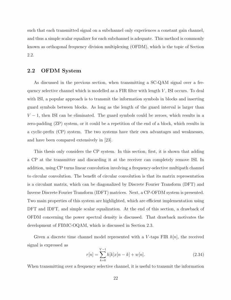
2.14 Transmission scheme using a CP. . . . . . . . . . . . . . . . . . . . . . . . . 23

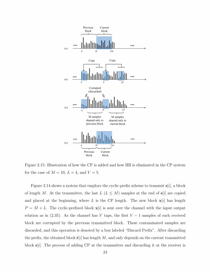
2.15 Illustration of how the CP is added and how IBI is eliminated in the CP

system for the case of M = 10, L = 4, and V = 5. . . . . . . . . . . . . . . . 24

2.16 Discrete-time OFDM system. . . . . . . . . . . . . . . . . . . . . . . . . . . 27

2.17 Equivalent parallel-subchannel model for the OFDM system. . . . . . . . . . 28

2.18 Frequency response of a rectangular pulse and its shifted version. . . . . . . 31

2.19 The OFDM transmitted signal synthesized from a bank of M filters. . . . . . 31

viii

2.20 Representation of an OFDM system in the continuous time domain. . . . . . 32

2.21 An illustration of how orthogonality is established in OFDM. . . . . . . . . . 33

2.22 Time-frequency phase-space lattice representation of an OFDM system. . . . 33

2.23 Block diagram of an FBMC-OQAM transmitter. . . . . . . . . . . . . . . . . 34

2.24 Block diagram of an FBMC-OQAM receiver. . . . . . . . . . . . . . . . . . . 35

2.25 Time frequency phase space for transmission of FBMC-OQAM system. . . . 36

2.26 The mth subcarrier channel in an FBMC-OQAM system. . . . . . . . . . . . 38

2.27 The interference branch from subcarrier (m+ 1) to subcarrier m. . . . . . . 39

2.28 Mangitude responses of the prototype filters and the estimated PSDs of OFDM

and FBMC-OQAM. M = 64 subcarriers, 32 active subcarriers which are

[17 : 48] , SRRC filter with roll-off factor β = 1 for FBMC-OQAM. . . . . . . 40

3.1 Block diagram of a GFDM transceiver. . . . . . . . . . . . . . . . . . . . . . 44

3.2 GFDM symbols obtained by linear convolution. . . . . . . . . . . . . . . . . 45

3.3 GFDM symbols obtained by circular convolution. . . . . . . . . . . . . . . . 46

3.4 Block structures of OFDM and GFDM systems for M = 5 and K = 4. . . . 48

3.5 Illustration of the impulse response of the GFDM system with K = 3, and

K = 4. . . . . . . . . . . . . . . . . . . . . . . . . . . . . . . . . . . . . . . . 50

3.6 ISI power versus the difference of m − m′ for RC and SRRC filters. g[n] is

obtained from a RC or SRRC filter with M = 9 symbols and K = 16 samples

per symbols. . . . . . . . . . . . . . . . . . . . . . . . . . . . . . . . . . . . . 52

3.8 Illustration of (3.24) for K = 3, and M = 2. . . . . . . . . . . . . . . . . . . 56

3.9 Efficient implementation of a GFDM system. . . . . . . . . . . . . . . . . . . 57

3.10 Comparison of implementation complexity of a GFDM system with K = 64. 58

ix

3.11 CFBMC-OQAM transmitted symbols after phase offset. . . . . . . . . . . . 60

3.12 Block diagram of the CFBMC-OQAM transceiver. . . . . . . . . . . . . . . . 61

3.13 ISI power versus the difference of m−m′, CFBMC-OQAM with SRRC, β =

0.9, K = 16, and M = 9. . . . . . . . . . . . . . . . . . . . . . . . . . . . . . 63

3.14 Illustration of the terms in (3.32) when M = 5, K = 8, SRRC filter with

β = 0.9, m′ = 0, and k − k′ = 1. . . . . . . . . . . . . . . . . . . . . . . . . . 64


β = 0.9, m′ = 3, and k − k′ = 3. . . . . . . . . . . . . . . . . . . . . . . . . . 65


β = 0.9, m′ = 0, and k − k′ = 2. . . . . . . . . . . . . . . . . . . . . . . . . . 66

3.17 The power of IICI,s versus k− k′ for various values of β, and M . K = 16, and

the filter is SRRC. . . . . . . . . . . . . . . . . . . . . . . . . . . . . . . . . 67


β = 0.9, m = 2, m′ = 3, k = 1, k′ = 2. One can see that nsym = 20 + 382−

(3− 2)84= 30. . . . . . . . . . . . . . . . . . . . . . . . . . . . . . . . . . . . 68

3.19 BER performance of OFDM, GFDM, and CFBMC-OQAM over AWGN chan-

nel. K = 64, M = 31, SRRC filter with β = 0.5. . . . . . . . . . . . . . . . . 69

3.21 Efficient implementation of a CFBMC-OQAM system. . . . . . . . . . . . . 73

4.1 Precoded CFBMC-OQAM system. . . . . . . . . . . . . . . . . . . . . . . . 75

4.2 Equivalent complex baseband WH-CFBMC-OQAM system. . . . . . . . . . 77

4.4 WH-CFBMC-OQAM and WH-GFDM BER performance over Channel A. . 85

4.5 WH-CFBMC-OQAM and WH-GFDM BER performance over Channel B. . 86

4.6 Simulation versus theoretical results of WH-CFBMC-OQAM system. . . . . 86

x

List of Tables

3.1 Impulse response of h1[n] and h2[n] . . . . . . . . . . . . . . . . . . . . . . . 70

4.1 ICI power (dB) for the example illustrated in Figure 4.3. . . . . . . . . . . . 81

4.2 Simulation parameters. . . . . . . . . . . . . . . . . . . . . . . . . . . . . . . 84

4.3 Delay profile used in simulation. . . . . . . . . . . . . . . . . . . . . . . . . . 84

xi

1. Introduction

Driven by the fast-growing demand in data traffic, research on enabling technologies for

the next (i.e., the fifth) generation of cellular networks, 5G networks, has been very active

during the past few years [1], [2]. Today, the use of powerful smartphones and tablets imposes

a high demand on advanced multimedia capabilities [3]. Since there are more users, devices,

and content, new innovative technologies that are efficient and intelligent are desired to

address many challenges, such as bandwidth shortage [4], high energy consumption [5], and

diverse quality of service requirements (QoS). The current cellular networks, 4G networks,

have reached the theoretical limit on the data rate with the current technologies and therefore

are not sufficient to cope with the above challenges. In developing 5G networks, three main

requirements have been identified [2], [3], [6]. First, a wide range of data rates has to be

supported, up to multiple gigabits per second, and tens of megabits per second need to be

guaranteed with very high availability and reliability. Second, a roundtrip latency of about

1 ms, an order of magnitude shorter than in 4G networks, is expected. Third, network

scalability and flexibility are required to support a large number of devices with very low

complexity and requirements for very long battery lifetime. Among ongoing research areas

that support these requirements, the modulation formats play an important role. They are

the key features for the past cellular generations, and yet again are expected to undergo

another major change in the upcoming fifth generation.

The fundamental design issues of the modulation formats are rooted in the random quality

of the wireless channels. Due to scattering, reflection and diffraction of the transmitted signal

caused by the presence of objects in the signal path, multiple versions of a transmitted signal

might reach the destination via multiple paths, called multipath propagation. An important

1

parameter of a wireless system is the multipath delay spread, defined as the difference in

propagation time between the longest and shortest paths [7]. When the delay spread is much

less than the symbol time, the channel is considered as flat, and a single tap is sufficient to

represent the channel. When the delay spread is larger than the symbol time, the channel

is said to be frequency-selective, and it has to be represented by multiple taps.

The frequency selectivity gives rise to intersymbol interference (ISI), where the received

symbol over a given symbol period experiences interference from other symbols that have

been delayed by multipath [8]. An approach to deal with the ISI problem is to design an

equalizer at the receiver that could compensate or reduce ISI [9]. However, the complexity of

the equalizer might increase dramatically when the channel is represented by so many taps.

For that reason, other approaches which require simpler equalizers are preferred. Multicar-

rier modulation is a well-known solution to serve that need. In fact, it is the dominating

modulation format for today’s wireless systems.

Multicarrier modulation is a method that divides a bit stream into multiple substreams

and sends them over many different subcarriers. By doing so, the data rate on each of

the subcarriers is much less than the total data rate, and the corresponding subcarrier

bandwidth is much smaller than the total system bandwidth. In particular, the number

of subcarriers should be chosen such that the subcarrier bandwidth is much less than the

coherence bandwidth of the channel, so that the individual subcarrier experiences a relatively

constant gain (i.e., flat channel) [8]. In short, multicarrier modulation decouples an ISI

(frequency-selective) channel into multiple parallel subchannels such that equalization and

detection at the receiver side can be done per subchannel.

Among many multicarrier techniques, orthogonal frequency division multiplexing (OFDM)

dominates the current broadband wireless communication systems [10]. OFDM can com-

pletely eliminate ISI through the use of a cyclic prefix, which consists of redundant symbols

replicated from the end to the beginning of each transmitted block. Further, OFDM offers

other advantages such as simple equalization by applying a scalar gain per subcarrier, and

efficient discrete-time implementation through fast Fourier transform (FFT). On the other

hand, OFDM also has its own drawbacks, such as high spectral leakage, high peak-to-average

2

power ratio (PARP), and strict orthogonality requirements.

Finding an appropriate multicarrier modulation technique for the next generation net-

works may be based on two approaches [10]. In the first approach, the existing OFDM

structure is preserved, and its drawbacks are addressed through appropriate solutions [11].

The second approach is based on a generalized framework for multicarrier systems [12], which

results in different techniques than OFDM.

Filter bank multicarrier communication offset QAM (FBMC-OQAM) is another candi-

date for 5G networks. Although, FBMC-OQAM has been invented even before OFDM, only

recently has FBMC-OQAM been considered as a promising technique, and drawn interest

from research community [12]. At the transmitter, FBMC-OQAM uses a set of filters, called

synthesis filter bank, to shape and then combine a set of input signals. At the receiver,

FBMC-OQAM uses another set of filters, called analysis filter bank, to split the received

signal into individual components. The OQAM modulation splits the complex data into real

and imaginary parts. By doing so, the orthogonality condition is relaxed and only applies

to the real field. This enables the use of flexible waveforms which leads to improvement

of signal’s power spectrum properties. These characteristics are the desired features for 5G

applications. However, FBMC-OQAM does not have a block-based structure as OFDM so

that CP can be inserted. This means that the subcarrier orthogonality could be destroyed

when the signal is transmitted through a frequency selective channel (FSC). In that case, an

equalizer with high complexity is needed at the receiver to compensate ISI.

Beside OFDM and FBMC-OQAM, there is another multicarrier scheme, called general-

ized frequency division multiplexing (GFDM), that has been recently proposed for the air

interface of the 5G networks [13]. GFDM has a block based structure and then CP can

be easily inserted. Further, GFDM exploits the block based structure to perform circular

convolution for pulse shaping rather than conventional linear convolution. By doing so, fil-

ters that are better than the rectangular filter can be utilized to improve the localization

property of the power spectrum density (PSD) of the transmitted signal without increasing

the CP length. However, the main issue of GFDM is that it is a nonorthogonal system,

and thus requiring an advanced receiver to reduce ISI and intercarrier interference (ICI). In

3

an additive white Gaussian noise (AWGN) channel, a matched filter receiver with iterative

interference cancellation can achieve almost the same symbol error rate performance as that

of OFDM [14].

Recently, circular FBMC-OQAM (CFBMC-OQAM), a modified version of FBMC-OQAM,

which makes use of circular convolution as in GFDM, has been proposed [15]. By using cir-

cular convolution, CFBMC-OQAM also has a block based structure, which enables the use

of CP to achieve free interblock interference (IBI), and eases the task of equalization at the

receiver. Furthermore, the circular convolution preserves the continuity of the transmitted

waveform within one block. That continuity is necessary to guarantee a good localized power

spectrum of the transmitted signal.

When operating over FSCs, the above multicarrier schemes do not offer any multipath

diversity due to the fact that each symbol is transmitted over a single flat subchannel that

may experience severe fading. Thus, the overall performance of the system is dominated

by the performance of badly affected subchannels if no additional technique to counteract

is applied. Precoding techniques are methods to solve such severe problem, and they have

been substantially studied for OFDM systems. In [16], precoded vector OFDM systems are

proposed for combating channel spectral nulls and reduce CP length. In [17], designs of linear

precoding to maximize diversity gain and coding gain are considered. Reference [18] proposes

the use of unitary precoders to minimize the bit error rate performance. In FBMC-OQAM

systems, a few precoding proposals have been presented in the literature. An analytical

approximation of the error performance of a precoded FBMC-OQAM system is establised

in [19] with the assumption that the transmission channel is perfectly equalized. Later, [20]

extends the previous study to the case where linear MMSE equalization is employed. For

GFDM systems, [21] investigates the use of a unitary matrix, the Walsh-Hadamard matrix, as

the precoder, and presents analytical approximation that can be used to estimate the bit error

rate of GFDM over frequency-selective channels. To the best of our knowledge, precoding

techniques and bit error rate performance of CFBMC-OQAM in frequency selective channels

have never been reported in the literature. Studying a precoding scheme that can improve

the overall bit error rate performance of CFBMC-OQAM system in FSCs is precisely the

4

main objective of this thesis.

The remainder of this chapter gives an overview of the thesis, its contributions and

organization.

In Chapter 2, background of single carrier and multicarrier wireless communication sys-

tems considered in this thesis is provided. In the single carrier systems, quadrature amplitude

modulation (QAM) and discrete time channel model are introduced. For multicarrier sys-

tems, the transceivers of OFDM and FBMC-OQAM are presented, in which the key features

of each system and the important differences between the two are discussed.

Chapter 3 presents two kinds of circular pulse-shaped waveforms for 5G networks, which

are GFDM and CFBMC-OQAM. For each system, the system model and its properties

are discussed, followed by the implementation structures. This chapter also highlights the

necessary of circular convolution and its usefulness in multicarrier systems. Further, the

similarities and differences between GFDM and CFBMC-OQAM are examined.

Chapter 4 investigates the combination of CFBMC-OQAM with WH transform, called

WH-CFBMC-OQAM, to improve the BER performance over FSCs. First, the system model

of WH-CFBMC-QOAM is introduced. The transceiver of a WH-CFBMC-OQAM system is

basically the same as that presented in Chapter 3 for CFBMC-OQAM except that a WH

precoder is applied at the transmitter side to perform a linear combination of the inputs, and

the Hermitian tranpose of the precoder is applied to the output at the receiver side to reverse

the precoding process. This chapter also derives the theoretical approximation for the BER

performance. The simulation results show that the WH-CFBMC-OQAM is superior than

WH-GFDM, and the theoretical results match well with the simulation results.

Finally, Chapter 5 draws conclusion and offers suggestions for further studies.

5

2. Background

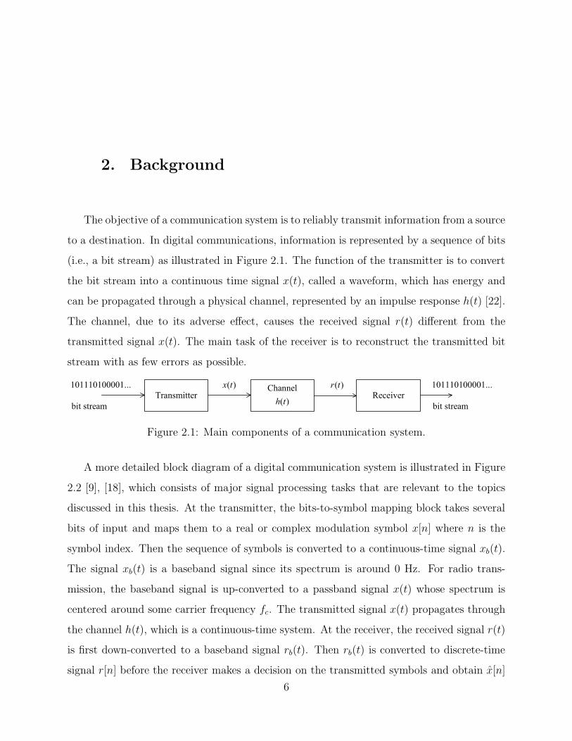
The objective of a communication system is to reliably transmit information from a source

to a destination. In digital communications, information is represented by a sequence of bits

(i.e., a bit stream) as illustrated in Figure 2.1. The function of the transmitter is to convert

the bit stream into a continuous time signal x(t), called a waveform, which has energy and

can be propagated through a physical channel, represented by an impulse response h(t) [22].

The channel, due to its adverse effect, causes the received signal r(t) different from the

transmitted signal x(t). The main task of the receiver is to reconstruct the transmitted bit

stream with as few errors as possible.

Transmitter ReceiverChannel

( )h tbit stream

101110100001...

bit stream

101110100001...( )x t ( )r t

Figure 2.1: Main components of a communication system.

A more detailed block diagram of a digital communication system is illustrated in Figure

2.2 [9], [18], which consists of major signal processing tasks that are relevant to the topics

discussed in this thesis. At the transmitter, the bits-to-symbol mapping block takes several

bits of input and maps them to a real or complex modulation symbol x[n] where n is the

symbol index. Then the sequence of symbols is converted to a continuous-time signal xb(t).

The signal xb(t) is a baseband signal since its spectrum is around 0 Hz. For radio trans-

mission, the baseband signal is up-converted to a passband signal x(t) whose spectrum is

centered around some carrier frequency fc. The transmitted signal x(t) propagates through

the channel h(t), which is a continuous-time system. At the receiver, the received signal r(t)

is first down-converted to a baseband signal rb(t). Then rb(t) is converted to discrete-time

signal r[n] before the receiver makes a decision on the transmitted symbols and obtain x[n]

6

h t

x n bx t x t

r tbr t r n x n

Figure 2.2: Block diagram of a digital communication system.

(symbol detection). Finally, the symbol-to-bits block maps the symbols x[n] back to the bit

stream.

This chapter will provide more details of the signal processing tasks that are illustrated

in Figure 2.2. First, a single-carrier QAM (SC-QAM) system is presented in Section 2.1.

The limitation of a single carrier system is discussed, which then motivates the development

of multicarrier systems. The well-known multicarrier system, orthogonal frequency division

multiplexing (OFDM), is presented in Section 2.2. An alternative multicarrier scheme, which

is based on the filter banks technique, called filter bank multicarrier offset QAM (FBMC-

OQAM), is presented in Section 2.3. A comparision between FBMC-OQAM and OFDM is

also provided in that section.

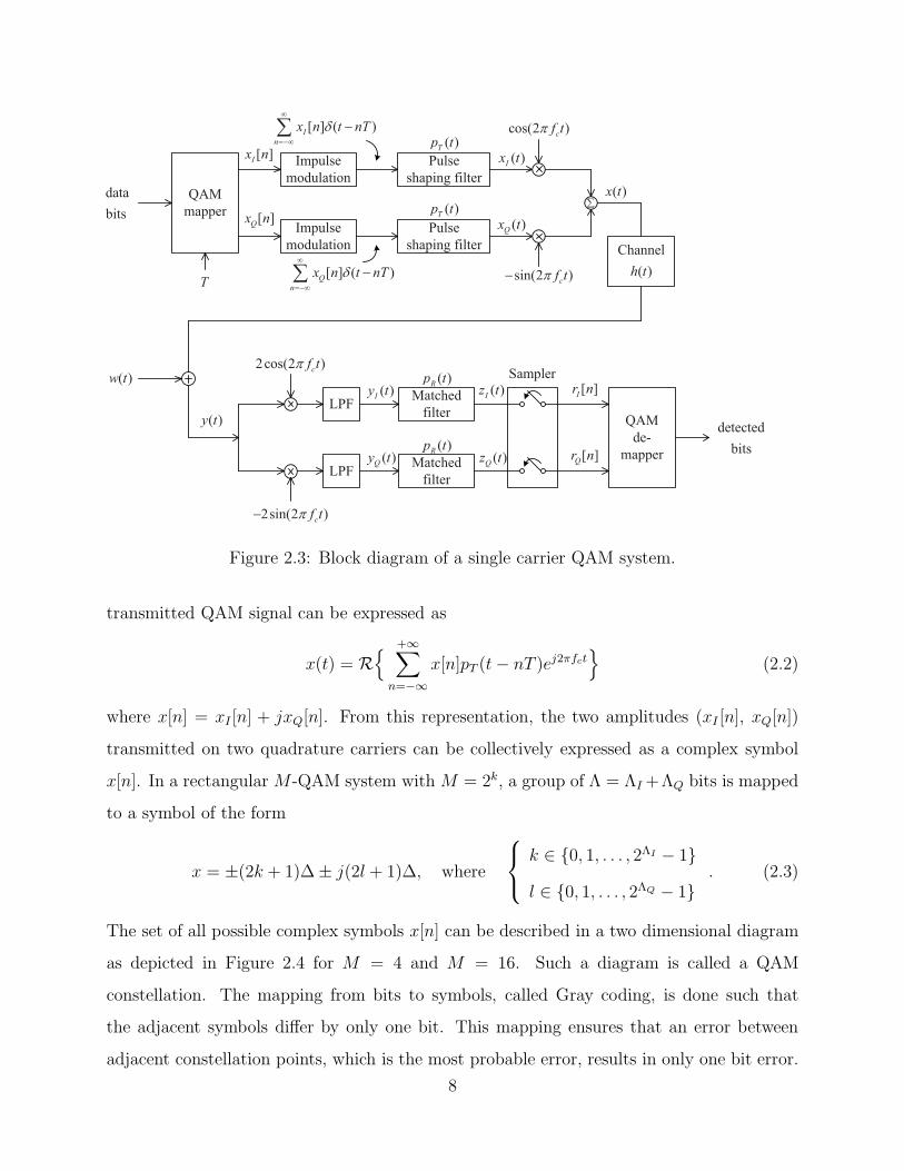
2.1 Single Carrier QAM System (SC-QAM)

Figure 2.3 illustrates a SC-QAM system. This system transmits two bit streams simulta-

neously by changing the amplitudes of two quadrature carriers, hence the name quadrature

amplitude modulation. The transmitted QAM signal can be expressed as

x(t) =+∞∑

n=−∞xI [n]pT (t− nT ) cos(2πfct)−

+∞∑

n=−∞xQ[n]pT (t− nT ) sin(2πfct) (2.1)

where xI [n] and xQ[n] are the signal amplitudes (which are real values) of the quadrature

carriers, pT (t) is the pulse shaping filter and T is the symbol period. Alternatively, the

7

Ix n

Qx n

h tT

I

n

x n t nT

Q

n

x n t nT

Tp t

Tp t

Ix t

Qx t

cf t

cf t

x t

w tcf t

cf t

Rp t

Rp tQy t

Iy t Iz t

Qz t

Ir n

Qr n

y t

Figure 2.3: Block diagram of a single carrier QAM system.

transmitted QAM signal can be expressed as

x(t) = R{ +∞∑

n=−∞x[n]pT (t− nT )ej2πfct

}

(2.2)

where x[n] = xI [n] + jxQ[n]. From this representation, the two amplitudes (xI [n], xQ[n])

transmitted on two quadrature carriers can be collectively expressed as a complex symbol

x[n]. In a rectangular M-QAM system with M = 2k, a group of Λ = ΛI +ΛQ bits is mapped

to a symbol of the form

x = ±(2k + 1)∆± j(2l + 1)∆, where

k ∈ {0, 1, . . . , 2ΛI − 1}

l ∈ {0, 1, . . . , 2ΛQ − 1}. (2.3)

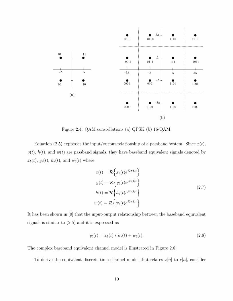
The set of all possible complex symbols x[n] can be described in a two dimensional diagram

as depicted in Figure 2.4 for M = 4 and M = 16. Such a diagram is called a QAM

constellation. The mapping from bits to symbols, called Gray coding, is done such that

the adjacent symbols differ by only one bit. This mapping ensures that an error between

adjacent constellation points, which is the most probable error, results in only one bit error.

8

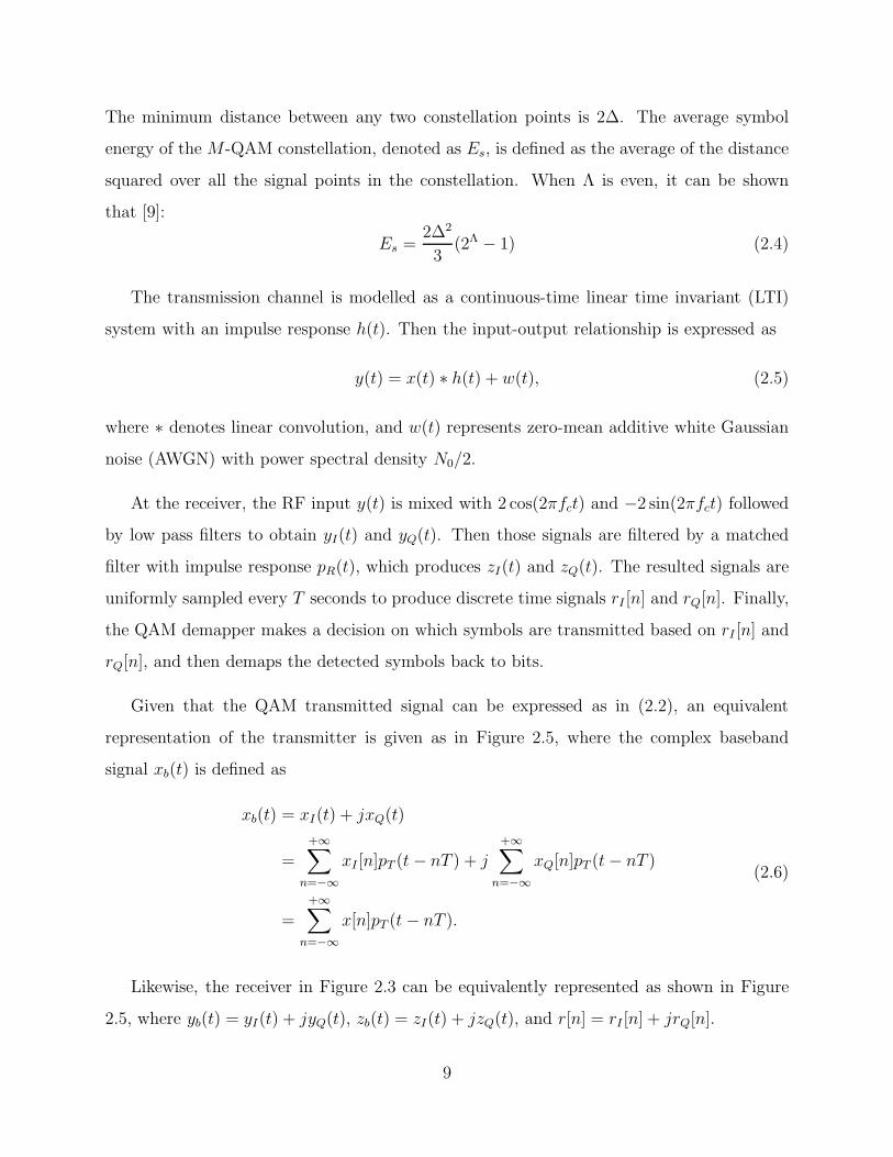
The minimum distance between any two constellation points is 2∆. The average symbol

energy of the M-QAM constellation, denoted as Es, is defined as the average of the distance

squared over all the signal points in the constellation. When Λ is even, it can be shown

that [9]:

Es =2∆2

3(2Λ − 1) (2.4)

The transmission channel is modelled as a continuous-time linear time invariant (LTI)

system with an impulse response h(t). Then the input-output relationship is expressed as

y(t) = x(t) ∗ h(t) + w(t), (2.5)

where ∗ denotes linear convolution, and w(t) represents zero-mean additive white Gaussian

noise (AWGN) with power spectral density N0/2.

At the receiver, the RF input y(t) is mixed with 2 cos(2πfct) and −2 sin(2πfct) followed

by low pass filters to obtain yI(t) and yQ(t). Then those signals are filtered by a matched

filter with impulse response pR(t), which produces zI(t) and zQ(t). The resulted signals are

uniformly sampled every T seconds to produce discrete time signals rI [n] and rQ[n]. Finally,

the QAM demapper makes a decision on which symbols are transmitted based on rI [n] and

rQ[n], and then demaps the detected symbols back to bits.

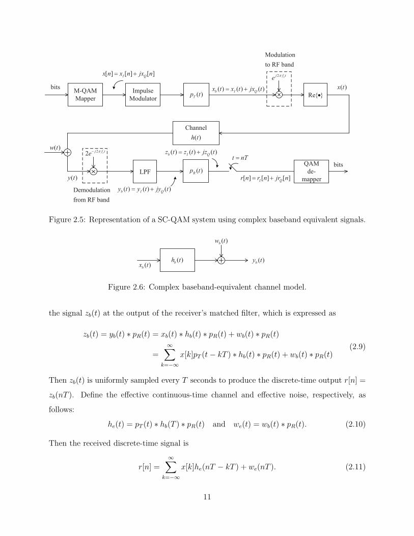
Given that the QAM transmitted signal can be expressed as in (2.2), an equivalent

representation of the transmitter is given as in Figure 2.5, where the complex baseband

signal xb(t) is defined as

xb(t) = xI(t) + jxQ(t)

=+∞∑

n=−∞xI [n]pT (t− nT ) + j

+∞∑

n=−∞xQ[n]pT (t− nT )

=

+∞∑

n=−∞x[n]pT (t− nT ).

(2.6)

Likewise, the receiver in Figure 2.3 can be equivalently represented as shown in Figure

2.5, where yb(t) = yI(t) + jyQ(t), zb(t) = zI(t) + jzQ(t), and r[n] = rI [n] + jrQ[n].

9

-D

00

01 11

10

D

(a)

(b)

Figure 2.4: QAM constellations (a) QPSK (b) 16-QAM.

Equation (2.5) expresses the input/output relationship of a passband system. Since x(t),

y(t), h(t), and w(t) are passband signals, they have baseband equivalent signals denoted by

xb(t), yb(t), hb(t), and wb(t) where

x(t) = R{

xb(t)ej2πfct

}

y(t) = R{

yb(t)ej2πfct

}

h(t) = R{

hb(t)ej2πfct

}

w(t) = R{

wb(t)ej2πfct

}

(2.7)

It has been shown in [9] that the input-output relationship between the baseband equivalent

signals is similar to (2.5) and it is expressed as

yb(t) = xb(t) ∗ hb(t) + wb(t). (2.8)

The complex baseband equivalent channel model is illustrated in Figure 2.6.

To derive the equivalent discrete-time channel model that relates x[n] to r[n], consider

10

h t

Tp tb I Qx t x t jx t

w t

x t

Rp t

I Qr n r n jr n

t nTb I Qz t z t jz t

b I Qy t y t jy t

cj f te

y t

I Qx n x n jx ncj f t

e

Figure 2.5: Representation of a SC-QAM system using complex baseband equivalent signals.

bh t

bw t

by tbx t

Figure 2.6: Complex baseband-equivalent channel model.

the signal zb(t) at the output of the receiver’s matched filter, which is expressed as

zb(t) = yb(t) ∗ pR(t) = xb(t) ∗ hb(t) ∗ pR(t) + wb(t) ∗ pR(t)

=

∞∑

k=−∞x[k]pT (t− kT ) ∗ hb(t) ∗ pR(t) + wb(t) ∗ pR(t)

(2.9)

Then zb(t) is uniformly sampled every T seconds to produce the discrete-time output r[n] =

zb(nT ). Define the effective continuous-time channel and effective noise, respectively, as

follows:

he(t) = pT (t) ∗ hb(T ) ∗ pR(t) and we(t) = wb(t) ∗ pR(t). (2.10)

Then the received discrete-time signal is

r[n] =∞∑

k=−∞x[k]he(nT − kT ) + we(nT ). (2.11)

11

h n

w n

r nx n

Figure 2.7: Equivalent discrete-time channel model.

The above expression can be rewritten as

r[n] =

∞∑

k=−∞x[k]h[n− k] + w[n], (2.12)

where h[n] and w[n] are, respectively, the discrete-time equivalent channel and noise given

by

h[n] = pT (t) ∗ hb(t) ∗ pR(t)∣∣∣t=nT

,

w[n] = wb(t) ∗ pR(t)∣∣∣t=nT

.(2.13)

Thus, the system shown in Figure 2.6 can be represented as in Figure 2.7, which contains

only discrete-time signals and system.

When an SC-QAM system operates in a channel with the input-output relationship

expressed as in (2.12), the received signal r[n] at time slot n not only depends on the

transmitted signal x[n], but also depends on the past symbols x[n − 1], x[n − 2], . . . . This

phenomenon is called intersymbol interference (ISI) and needs to be addressed. In the

following, one approach to deal with ISI in an SC-QAM system is presented.

Equation (2.12) can be rewritten as

r[n] = x[n]h[0] +∑

k 6=n

x[k]h[n− k] + w[n], (2.14)

where the term x[n]h[0] is the desired information symbol at the time slot n, and the term∑

k 6=n x[k]h[n− k] represents ISI. It is noted that h[n] is the sample of he(t) = pT (t) ∗ hb(t) ∗pR(t) at time slot n. Thus, in order to have zero ISI, one should have

he(nT ) =

1, n = 0

0, otherwise. (2.15)

12

Denote He(f) as the frequency response of he(t). Then the condition in (2.15) is satisfied

if [22]∞∑

n=−∞He

(

f +n

T

)

= T for |f | ≤ 1

2T. (2.16)

Equation (2.16) means that if one designs he(t) such that He(f) and its aliases (resulted

from sampling he(t)) add up to a constant value in frequency band |f | ≤ 1/2T , then zero

ISI is achieved. This is known as Nyquist’s first criterion.

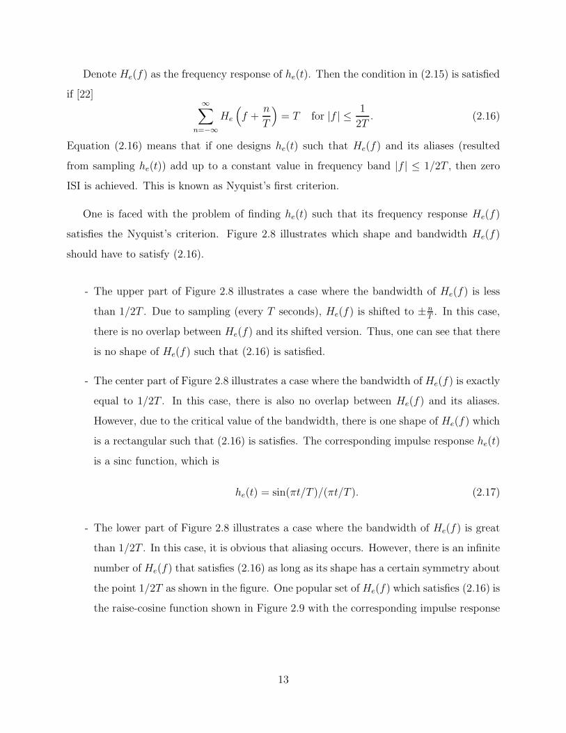
One is faced with the problem of finding he(t) such that its frequency response He(f)

satisfies the Nyquist’s criterion. Figure 2.8 illustrates which shape and bandwidth He(f)

should have to satisfy (2.16).

- The upper part of Figure 2.8 illustrates a case where the bandwidth of He(f) is less

than 1/2T . Due to sampling (every T seconds), He(f) is shifted to ± nT. In this case,

there is no overlap between He(f) and its shifted version. Thus, one can see that there

is no shape of He(f) such that (2.16) is satisfied.

- The center part of Figure 2.8 illustrates a case where the bandwidth of He(f) is exactly

equal to 1/2T . In this case, there is also no overlap between He(f) and its aliases.

However, due to the critical value of the bandwidth, there is one shape of He(f) which

is a rectangular such that (2.16) is satisfies. The corresponding impulse response he(t)

is a sinc function, which is

he(t) = sin(πt/T )/(πt/T ). (2.17)

- The lower part of Figure 2.8 illustrates a case where the bandwidth of He(f) is great

than 1/2T . In this case, it is obvious that aliasing occurs. However, there is an infinite

number of He(f) that satisfies (2.16) as long as its shape has a certain symmetry about

the point 1/2T as shown in the figure. One popular set ofHe(f) which satisfies (2.16) is

the raise-cosine function shown in Figure 2.9 with the corresponding impulse response

13

eH f eH fT

eH fT

eH fT

eH f eH fT

eH fT

eH fT

T T T TTT

T T T TTT

eH f eH fT

eH fT

eH fT

T T T TTT

e

n

nH f

T

TT

Figure 2.8: Condition on He(f) to achieve zero ISI.

shown in Figure 2.10. It is given as [22]

He(f) = HRC(f) =

T, |f | ≤ 1−β2T

T cos2[πT2β

(|f | − 1−β

2T

)]

, 1−β2T

≤ |f | ≤ 1+β2T

0, |f | ≥ 1+β2T

. (2.18)

14

fT-1 -0.8 -0.6 -0.4 -0.2 0 0.2 0.4 0.6 0.8 1

He(f)

0

0.1

0.2

0.3

0.4

0.5

0.6

0.7

0.8

0.9

1

β=0β=0.5β=1

Figure 2.9: The raised-cosine spectrum

The impulse response is given by

he(t) = sinc(t/T )cos(πβt/T )

1− 4β2t2/T 2, (2.19)

where β is the roll-off factor, which controls the excess bandwidth.

t/T-3 -2 -1 0 1 2 3

he(t)

-0.05

0

0.05

0.1

0.15

0.2

0.25

0.3

β=0β=0.5β=1

Figure 2.10: Time domain function of the raised-cosine spectrum

Recall that He(f) = HT (f)Hb(f)HR(f) is the overall frequency response and one knows

what He(f) must be such that zero-ISI is achieved. For a given choice of a Hb(f), such as

a raised-cosine spectrum, one still needs to find out what are the optimal designs of HT (f)

15

and HR(f). However, the optimal design in what sense should be stated first. It is noted

that the design of HR(f) not only affects the ISI term but also the noise. It will be shown

later that the probability of error is determined by the signal-to-noise ratio (SNR). Thus,

the choice of HR(f) affects the probability of error. Therefore, the design problem is an

optimization problem which is stated

minimizeHT (f),HR(f)

probability of error

subject to transmitted power PT

HT (f)Hb(f)HR(f) satisfies zero-ISI criterion

(2.20)

If the noise has a flat PSD over the channel bandwidth, then the solution for the above

problem is given as [22]

|HR(f)|2 = K1|He(f)||Hb(f)|

,

|HT (f)|2 = K2|He(f)||Hb(f)|

=K2

K1|HR(f)|2,

(2.21)

where K1, and K2 are arbitrary constant which set the power levels at the transmitter and

the receiver. In addition, the phases of HT (f) and HR(f) should cancel each other, which

implies that the transmit and receive filters are a matched-filter pair.

In the special case where the channel is ideal, i.e., Hb(f) = 1 for |f | ≤ W where W is

the channel bandwidth and K1 = K2, one obtains |HT (f)| = |HR(f)| =√

|He(f)|/√K1.

If He(f) is a raise-cosine spectrum and K1 = 1, then HT (f) and HR(f) are square-root

raised-cosine (SRRC) spectrum:

HT (f) = HR(f) =

√T , |f | ≤ 1−β

2T

√T cos

[πT2β

(|f | − 1−β

2T

)]

, 1−β2T

≤ |f | ≤ 1+β2T

0, |f | ≥ 1+β2T

. (2.22)

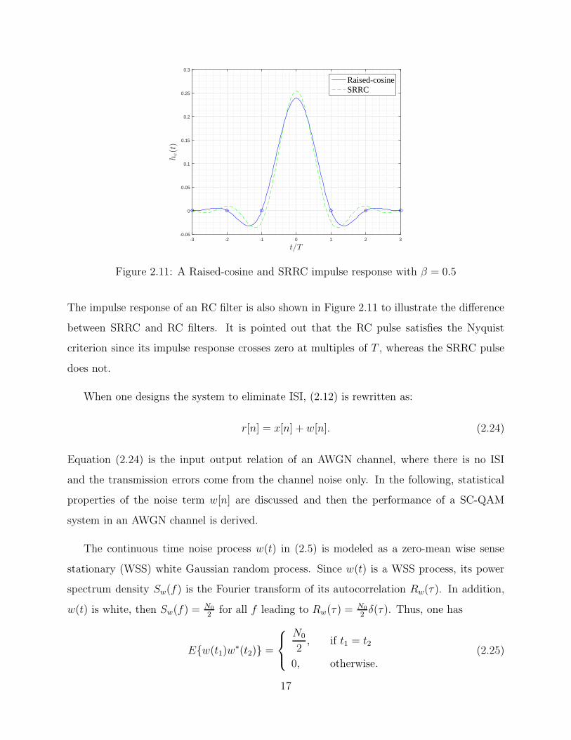
The impulse response of SRRC is shown in Figure 2.11 and is given as [22]

hT (t) = hR(t) =4βt/T cos[π(1 + β)t/T ] + sin[π(1− β)t/T ]

(πt/T )[1− (4βt/T )2](2.23)

16

t/T-3 -2 -1 0 1 2 3

he(t)

-0.05

0

0.05

0.1

0.15

0.2

0.25

0.3

Raised-cosineSRRC

Figure 2.11: A Raised-cosine and SRRC impulse response with β = 0.5

The impulse response of an RC filter is also shown in Figure 2.11 to illustrate the difference

between SRRC and RC filters. It is pointed out that the RC pulse satisfies the Nyquist

criterion since its impulse response crosses zero at multiples of T , whereas the SRRC pulse

does not.

When one designs the system to eliminate ISI, (2.12) is rewritten as:

r[n] = x[n] + w[n]. (2.24)

Equation (2.24) is the input output relation of an AWGN channel, where there is no ISI

and the transmission errors come from the channel noise only. In the following, statistical

properties of the noise term w[n] are discussed and then the performance of a SC-QAM

system in an AWGN channel is derived.

The continuous time noise process w(t) in (2.5) is modeled as a zero-mean wise sense

stationary (WSS) white Gaussian random process. Since w(t) is a WSS process, its power

spectrum density Sw(f) is the Fourier transform of its autocorrelation Rw(τ). In addition,

w(t) is white, then Sw(f) =N0

2for all f leading to Rw(τ) =

N0

2δ(τ). Thus, one has

E{w(t1)w∗(t2)} =

N0

2, if t1 = t2

0, otherwise.(2.25)

17

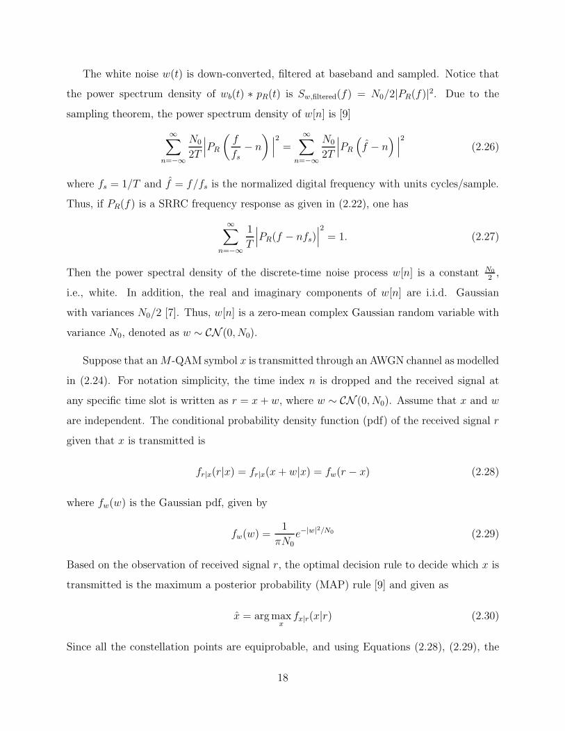
The white noise w(t) is down-converted, filtered at baseband and sampled. Notice that

the power spectrum density of wb(t) ∗ pR(t) is Sw,filtered(f) = N0/2|PR(f)|2. Due to the

sampling theorem, the power spectrum density of w[n] is [9]

∞∑

n=−∞

N0

2T

∣∣∣PR

(f

fs− n

) ∣∣∣

2

=

∞∑

n=−∞

N0

2T

∣∣∣PR

(

f − n) ∣∣∣

2

(2.26)

where fs = 1/T and f = f/fs is the normalized digital frequency with units cycles/sample.

Thus, if PR(f) is a SRRC frequency response as given in (2.22), one has

∞∑

n=−∞

1

T

∣∣∣PR(f − nfs)

∣∣∣

2

= 1. (2.27)

Then the power spectral density of the discrete-time noise process w[n] is a constant N0

2,

i.e., white. In addition, the real and imaginary components of w[n] are i.i.d. Gaussian

with variances N0/2 [7]. Thus, w[n] is a zero-mean complex Gaussian random variable with

variance N0, denoted as w ∼ CN (0, N0).

Suppose that anM-QAM symbol x is transmitted through an AWGN channel as modelled

in (2.24). For notation simplicity, the time index n is dropped and the received signal at

any specific time slot is written as r = x+ w, where w ∼ CN (0, N0). Assume that x and w

are independent. The conditional probability density function (pdf) of the received signal r

given that x is transmitted is

fr|x(r|x) = fr|x(x+ w|x) = fw(r − x) (2.28)

where fw(w) is the Gaussian pdf, given by

fw(w) =1

πN0e−|w|2/N0 (2.29)

Based on the observation of received signal r, the optimal decision rule to decide which x is

transmitted is the maximum a posterior probability (MAP) rule [9] and given as

x = argmaxx

fx|r(x|r) (2.30)

Since all the constellation points are equiprobable, and using Equations (2.28), (2.29), the

18

r

Figure 2.12: Minimum-distance decision regions of 16-QAM.

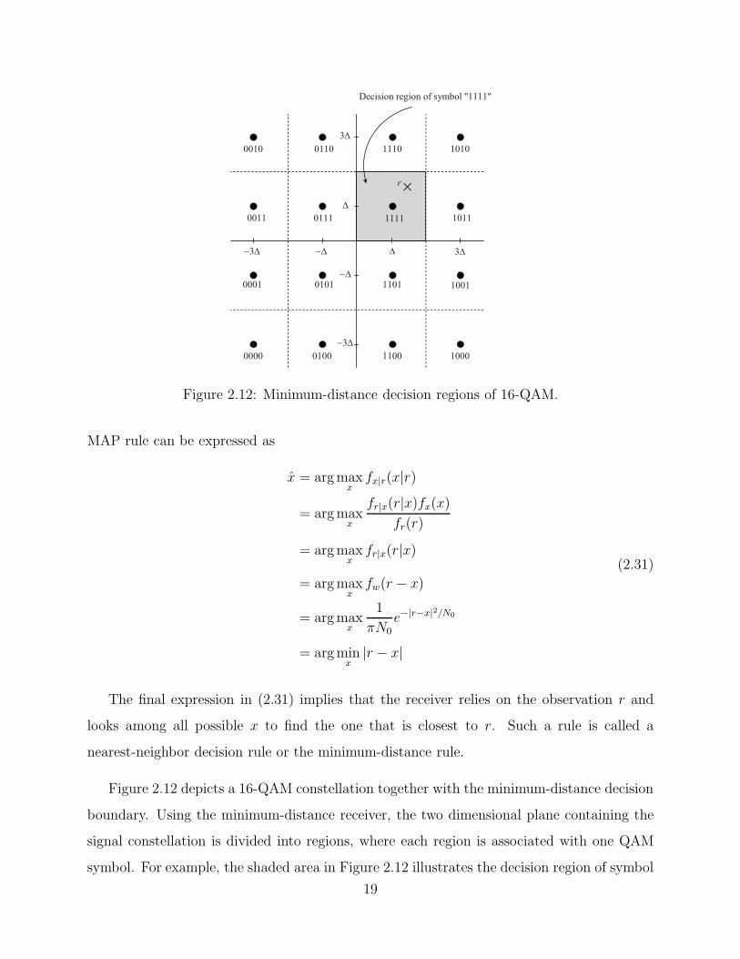
MAP rule can be expressed as

x = argmaxx

fx|r(x|r)

= argmaxx

fr|x(r|x)fx(x)fr(r)

= argmaxx

fr|x(r|x)

= argmaxx

fw(r − x)

= argmaxx

1

πN0e−|r−x|2/N0

= argminx

|r − x|

(2.31)

The final expression in (2.31) implies that the receiver relies on the observation r and

looks among all possible x to find the one that is closest to r. Such a rule is called a

nearest-neighbor decision rule or the minimum-distance rule.

Figure 2.12 depicts a 16-QAM constellation together with the minimum-distance decision

boundary. Using the minimum-distance receiver, the two dimensional plane containing the

signal constellation is divided into regions, where each region is associated with one QAM

symbol. For example, the shaded area in Figure 2.12 illustrates the decision region of symbol

19

SNR per bit, Eb/N0 [dB]0 2 4 6 8 10 12 14 16 18 20

Biterrorrate,Pb

10-6

10-5

10-4

10-3

10-2

10-1

100

QPSK16-QAM64-QAM

Figure 2.13: Bit error rates for different QAM systems.

(1111). The received signal r, due to noise, could be a random point in the two dimension

plane. If r falls into the shaded area, then the QAM symbol (1111) is decided to be the

transmitted symbol.

To derive the probability of error for a QAM system under an AWGN channel, one

must specify the signal constellation. This thesis considers rectangular QAM constellations.

Although they are not the best M-QAM signal constellations for M ≥ 16, the average

transmitted power required to achieve a given minimum distance is only slighly greater than

the average power required for the best M-QAM signal constellation [9]. In addition, a

rectangular QAM signal constellation has the distinct advantage of being easily generated

as two ASK signals transmitted on the in-phase and quadrature carriers.

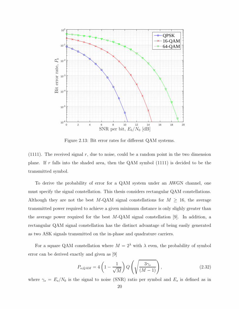
For a square QAM constellation where M = 2λ with λ even, the probability of symbol

error can be derived exactly and given as [9]

Ps,QAM = 4

(

1− 1√M

)

Q

(√

3γs(M − 1)

)

, (2.32)

where γs = Es/N0 is the signal to noise (SNR) ratio per symbol and Es is defined as in

20

(2.4). If one uses Gray mapping to map the real and imaginary parts, respectively, any

QAM symbol and its neighbors will differ only by one bit. In this case, the bit error rate

(BER) of the M-QAM system can be approximated by

Pb,QAM =1

log2(M)Ps,QAM .

=4

log2(M)

(

1− 1√M

)

Q

(√

3γb log2(M)

(M − 1)

)

,

(2.33)

where γb = γs/ log2(M) is the SNR per bit.

Figure 2.13 shows the BER plots of QPSK, 16-QAM, and 64-QAM systems under the

AWGN channel. Notice that to achieve the same level of error rate the QAM system with

larger M requires more power. For example, at the level of Pb = 10−6, the gap between 16-

QAM and 64-QAM is around 5dB. This means that the transmit power needs to be increased

by 5dB in order to send two additional bits per symbol while maintaining the same quality

of service, at Pb = 10−6.

Designing the transmit and receive filters as discussed is one approach to deal with ISI.

Another approach is that one does not design the system to eliminate ISI but design the

demodulator, with the ISI present, that best reconstructs the transmitted sequence [22]. Ref-

erence [9] demonstrates that an optimum demodulator can be realized as a filter matched

to the overall impulse response of the chain: modulator/transmit filter/channel, followed

by a sampler operating at the symbol rate and subsequent maximum-likelihood (ML) de-

tection for estimating the transmitted sequence from the sample values. The optimal ML

detection can be implemented using the Viterbi algorithm. However, the complexity of the

Viterbi algorithm grows exponentially with the number of channel taps. Alternatively, sub-

optimal demodulators which have lower complexity and yield comparable performance can

be considered. Some candidates are linear equalizers such as the zero-forcing and minimum

mean square error equalizers, which involve simple linear operations on the received symbols

followed by simple hard detection.

Another popular alternate approach to deal with ISI is to use signal processing techniques

at the transmitter and receiver to convert the ISI channel into non ISI parallel subchannels

21

such that each transmitted signal on a subchannel only experiences a constant gain channel,

and thus a simple scalar equalizer for each subchannel is adequate. This method is commonly

known as orthogonal frequency division multiplexing (OFDM), which is the topic of Section

2.2.

2.2 OFDM System

As discussed in the previous section, when transmitting a SC-QAM signal over a fre-

quency selective channel which is modelled as a FIR filter with length V , ISI occurs. To deal

with ISI, a popular approach is to transmit the information symbols in blocks and inserting

guard symbols between blocks. As long as the length of the guard interval is larger than

V − 1, then ISI can be eliminated. The guard symbols could be zeroes, which results in a

zero-padding (ZP) system, or it could be a repetition of the end of a block, which results in

a cyclic-prefix (CP) system. The two systems have their own advantages and weaknesses,

and have been compared extensively in [23].

This thesis only considers the CP system. In this section, first, it is shown that adding

a CP at the transmitter and discarding it at the receiver can completely remove ISI. In

addition, using CP turns linear convolution involving a frequency-selective multipath channel

to circular convolution. The benefit of circular convolution is that its matrix representation

is a circulant matrix, which can be diagonalized by Discrete Fourier Transform (DFT) and

Inverse Discrete Fourier Transform (IDFT) matrices. Next, a CP-OFDM system is presented.

Two main properties of this system are highlighted, which are efficient implementation using

DFT and IDFT, and simple scalar equalization. At the end of this section, a drawback of

OFDM concerning the power spectral density is discussed. That drawback motivates the

development of FBMC-OQAM, which is discussed in Section 2.3.

Given a discrete time channel model represented with a V -taps FIR h[n], the received

signal is expressed as

r[n] =

V−1∑

k=0

h[k]x[n− k] + w[n]. (2.34)

When transmitting over a frequency selective channel, it is useful to transmit the information

22

Cyclic PrefixDiscard

Prefix

Channel

[ ]h n

[ ]s n [ ]x n [ ]r n [ ]r n

Figure 2.14: Transmission scheme using a CP.

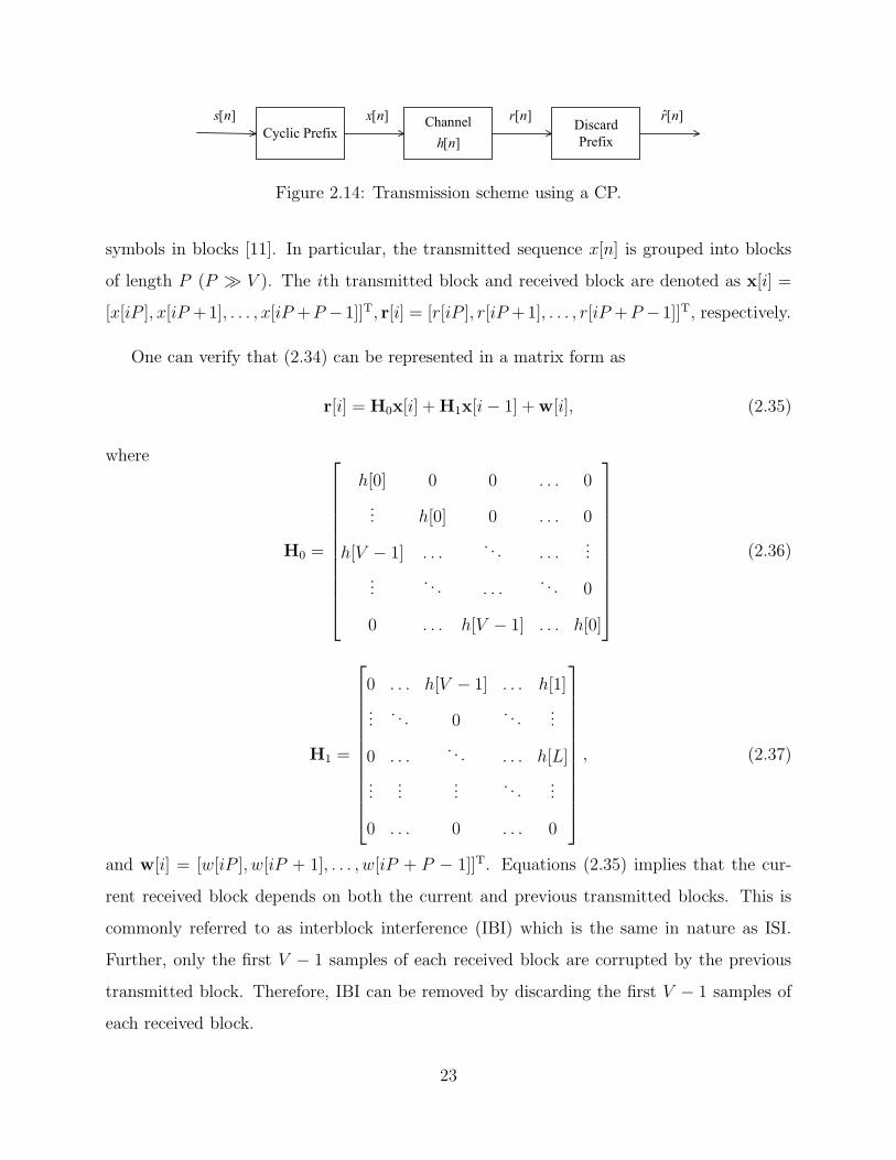
symbols in blocks [11]. In particular, the transmitted sequence x[n] is grouped into blocks

of length P (P ≫ V ). The ith transmitted block and received block are denoted as x[i] =

[x[iP ], x[iP +1], . . . , x[iP +P −1]]T, r[i] = [r[iP ], r[iP +1], . . . , r[iP +P −1]]T, respectively.

One can verify that (2.34) can be represented in a matrix form as

r[i] = H0x[i] +H1x[i− 1] +w[i], (2.35)

where

H0 =

h[0] 0 0 . . . 0

... h[0] 0 . . . 0

h[V − 1] . . .. . . . . .

...

.... . . . . .

. . . 0

0 . . . h[V − 1] . . . h[0]

(2.36)

H1 =

0 . . . h[V − 1] . . . h[1]

.... . . 0

. . ....

0 . . .. . . . . . h[L]

......

.... . .

...

0 . . . 0 . . . 0

, (2.37)

and w[i] = [w[iP ], w[iP + 1], . . . , w[iP + P − 1]]T. Equations (2.35) implies that the cur-

rent received block depends on both the current and previous transmitted blocks. This is

commonly referred to as interblock interference (IBI) which is the same in nature as ISI.

Further, only the first V − 1 samples of each received block are corrupted by the previous

transmitted block. Therefore, IBI can be removed by discarding the first V − 1 samples of

each received block.

23

Current

block

Previous

block

M samples

depend only to

current block

M samples

depend only to

previous block

Corrupted

(discarded)

Copy Copy

Current

block

Previous

block

[ ]s n

[ ]x n

[ ]r n

ˆ[ ]r n

0 M 2M

0 P 2P

0 P 2P

0 M 2M

···

···

···

··· ···

···

···

···

Figure 2.15: Illustration of how the CP is added and how IBI is eliminated in the CP system

for the case of M = 10, L = 4, and V = 5.

Figure 2.14 shows a system that employs the cyclic-prefix scheme to transmit s[i], a block

of length M . At the transmitter, the last L (L ≤ M) samples at the end of s[i] are copied

and placed at the beginning, where L is the CP length. The new block x[i] has length

P = M + L. The cyclic-prefixed block x[i] is sent over the channel with the input output

relation as in (2.35). As the channel has V taps, the first V − 1 samples of each received

block are corrupted by the previous transmitted block. These contaminated samples are

discarded, and this operation is denoted by a box labeled “Discard Prefix”. After discarding

the prefix, the obtained block r[i] has lengthM , and only depends on the current transmitted

block s[i]. The process of adding CP at the transmitter and discarding it at the receiver is

24

illustrated in Figure 2.15. The length of the CP is chosen such that L ≥ V − 1 in order to

completely eliminate IBI.

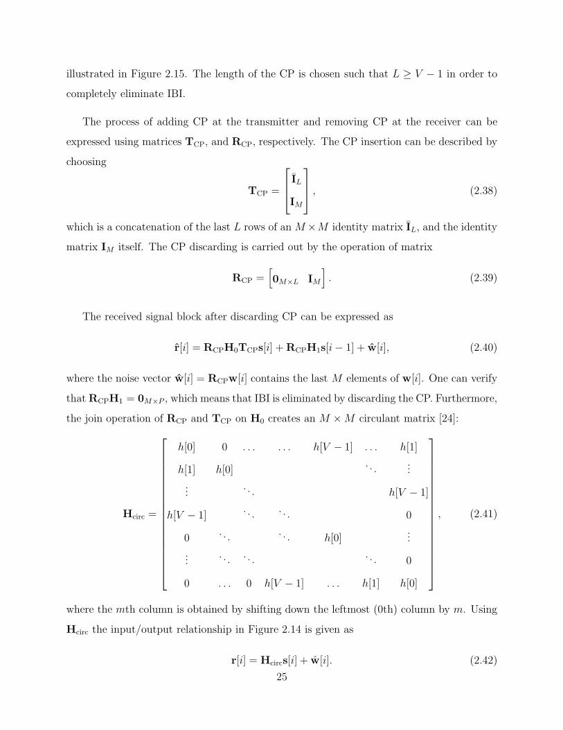
The process of adding CP at the transmitter and removing CP at the receiver can be

expressed using matrices TCP, and RCP, respectively. The CP insertion can be described by

choosing

TCP =

IL

IM

, (2.38)

which is a concatenation of the last L rows of an M×M identity matrix IL, and the identity

matrix IM itself. The CP discarding is carried out by the operation of matrix

RCP =[

0M×L IM

]

. (2.39)

The received signal block after discarding CP can be expressed as

r[i] = RCPH0TCPs[i] +RCPH1s[i− 1] + w[i], (2.40)

where the noise vector w[i] = RCPw[i] contains the last M elements of w[i]. One can verify

thatRCPH1 = 0M×P , which means that IBI is eliminated by discarding the CP. Furthermore,

the join operation of RCP and TCP on H0 creates an M ×M circulant matrix [24]:

Hcirc =

h[0] 0 . . . . . . h[V − 1] . . . h[1]

h[1] h[0]. . .

...

.... . . h[V − 1]

h[V − 1]. . .

. . . 0

0. . .

. . . h[0]...

.... . .

. . .. . . 0

0 . . . 0 h[V − 1] . . . h[1] h[0]

, (2.41)

where the mth column is obtained by shifting down the leftmost (0th) column by m. Using

Hcirc the input/output relationship in Figure 2.14 is given as

r[i] = Hcircs[i] + w[i]. (2.42)

25

It should be noted that the operation Hcircs[i] is equivalent to circular convolution of s[i]

and the leftmost column of Hcirc [25]. Therefore, Equation (2.42) shows that by inserting

the CP at the transmitter and discarding the CP at the receiver, the linear convolution with

the channel (which results in IBI) in (2.35) is converted to a circular convolution and IBI is

eliminated.

The matrix Hcirc can be diagonalized by DFT and IDFT matrices as

Hcirc = FHΓF, (2.43)

where the M ×M DFT matrix F is a matrix whose (k,m)th element is given as

[F]k,m =1√M

e−j2πkm/M , (2.44)

and Γ is the diagonal matrix

Γ =

H0 0 . . . 0

0 H1 . . . 0

......

. . ....

0 0 . . . HM−1

. (2.45)

The quantity Hl is the lth DFT coefficient of h[n]:

Hl =

M−1∑

n=0

h[n]e−j2πnl/M . (2.46)

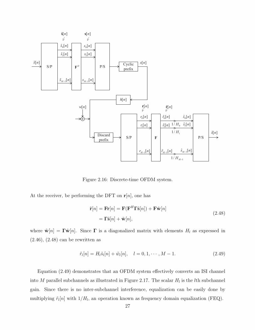
Figure 2.16 shows the block diagram of a system, known as OFDM, that takes advantage

of the circular channel matrix as given in (2.43). In this system, the information sequence s[n]

is first demultiplexed intoM−1 streams such that the lth stream is given as sl[n] = s[nM+l].

A block of symbols at time n is given an s[n] = [s0[n], s1[n], · · · , sM−1[n]]. The vector sn

is processed (precoded) by FH to produce s[n] = FH s[n]. Then, the CP system is applied

to s[n]. Substituting s[n] = FH s[n] and Hcirc = FHΓF into (2.42) the nth received signal

vector is expressed as

r[n] = (FHΓF)FH s[n] + w[n]

= FHΓs[n] + w[n].(2.47)

26

H

h n

w n

x n

s ns n

s n

s n

Ms n

H

H

MH

n n

s n

s n

Ms n

n

s n

Ms n

n

r n

r n

Mr n

r n

r n

Mr n

s n

Figure 2.16: Discrete-time OFDM system.

At the receiver, be performing the DFT on r[n], one has

r[n] = Fr[n] = F(FHΓs[n]) + Fw[n]

= Γs[n] + w[n],(2.48)

where w[n] = Γw[n]. Since Γ is a diagonalized matrix with elements Hl as expressed in

(2.46), (2.48) can be rewritten as

rl[n] = Hlsl[n] + wl[n], l = 0, 1, · · · ,M − 1. (2.49)

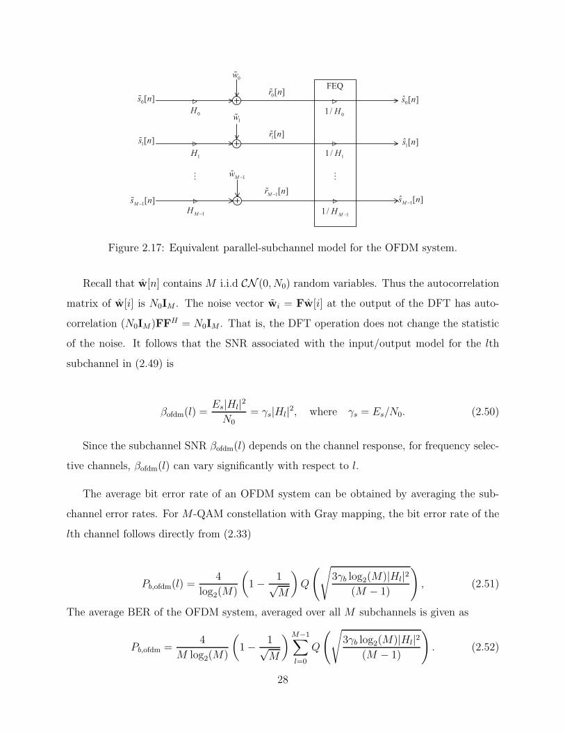
Equation (2.49) demonstrates that an OFDM system effectively converts an ISI channel

into M parallel subchannels as illustrated in Figure 2.17. The scalar Hl is the lth subchannel

gain. Since there is no inter-subchannel interference, equalization can be easily done by

multiplying rl[n] with 1/Hl, an operation known as frequency domain equalization (FEQ).

27

s nr n

s n

H

w

H

s n

HH

Ms n

MHMH

w

Mw

s n

Ms n

r n

Mr n

Figure 2.17: Equivalent parallel-subchannel model for the OFDM system.

Recall that w[n] contains M i.i.d CN (0, N0) random variables. Thus the autocorrelation

matrix of w[i] is N0IM . The noise vector wi = Fw[i] at the output of the DFT has auto-

correlation (N0IM)FFH = N0IM . That is, the DFT operation does not change the statistic

of the noise. It follows that the SNR associated with the input/output model for the lth

subchannel in (2.49) is

βofdm(l) =Es|Hl|2N0

= γs|Hl|2, where γs = Es/N0. (2.50)

Since the subchannel SNR βofdm(l) depends on the channel response, for frequency selec-

tive channels, βofdm(l) can vary significantly with respect to l.

The average bit error rate of an OFDM system can be obtained by averaging the sub-

channel error rates. For M-QAM constellation with Gray mapping, the bit error rate of the

lth channel follows directly from (2.33)

Pb,ofdm(l) =4

log2(M)

(

1− 1√M

)

Q

(√

3γb log2(M)|Hl|2(M − 1)

)

, (2.51)

The average BER of the OFDM system, averaged over all M subchannels is given as

Pb,ofdm =4

M log2(M)

(

1− 1√M

)M−1∑

l=0

Q

(√

3γb log2(M)|Hl|2(M − 1)

)

. (2.52)

28

As demonstrated, CP plays an important role in an OFDM system. However, CP leads

to bandwidth inefficiency. Transmitting an information block of length M requires a block

of length M + L, which results in a reduced bandwidth efficiency of η = M/(M + L).

In a frequency selective channel with a large number of taps, L should be long enough

to combat IBI leading to small η. One could increase M such that M ≫ L to have an

expected η. However, largeM increases the delay of the system as well as the implementation

complexity. Therefore, CP length needs to be carefully chosen when operating CP-OFDM in

frequency selective channels, especially in cellular communication channels where bandwidth

is a valuable resource.

Another drawback of OFDM system is inefficiency in using bandwidth since guard bands

need to be allocated to prevent interference between communication system (which use

OFDM transmission) operating in adjacent bands. This is due to the high side lobes of the

spectrum of the transmitted signal. This is shown in the following.

From Figure (2.16), the transmitted signal on each subcarrier can be expressed as

sk[n] =1√M

M−1∑

l=0

sl[n]ej2πkl/M (2.53)

The signal sequence x[n] (assume no CP is added for simplicity) after the P/S converter is

x[n] =

M−1∑

k=0

[sk[n− k]]↑M , (2.54)

where [•]↑M denotes the upsampling by M samples of the sequence inside the bracket [26].

From (2.53), (2.54), the z transform of x[n] is given as

X(z) =

M−1∑

k=0

Sk(zM)z−k

=M−1∑

k=0

1√M

M−1∑

m=0

Sl(zM )ej2πkl/Mz−k

=1√M

M−1∑

l=0

Sl(zM )

M−1∑

k=0

(zej2πl/M

)−k

=1√M

M−1∑

l=0

Sl(zM )Fl(z),

(2.55)

29

where

Fl(z) = F0(zej2πl/M )

F0(z) = 1 + z−1 + . . .+ z−(M−1)(2.56)

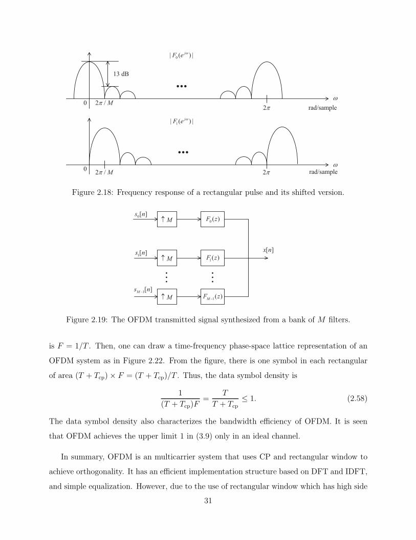
Equation (2.55) shows that the frequency spectrum of the lth subcarrier signal is compressed

by M and then passes through the filter Fl(z). In addition, (2.56) implies f0[n] is a rectan-

gular window and |F0(ejω)| = | sin(Mω/2)/ sin(ω/2)|, which is plotted in Figure 2.18. The

filter Fl[z] has response

Fl(ejω) = F0(e

j(ω−(2πl/M))) (2.57)

which is a shifted version of F0(ejω). Thus, one can conclude that the transmitted OFDM

signal can be synthesized from a bank of M filters as illustrated in Figure 2.19. The M filters

are obtained from a single filter F0(z) by uniformly shifting the response. The stop-band

attenuation of F0(z) is around 13 dB and its stop-band decays slowly with frequency.

To address the high stop-band attenuation, one could design F0(z) that has a sharper

cutoff and higher stopband attenuation. However, in that case f0[n] is no longer an rectan-

gular window and the CP length of the OFDM system should add to the length of f0[n] to

guarantee no IBI [24]. Longer length of CP reduces the spectrum efficiency and should be

avoided. Alternate multicarrier systems that do not require CP to achieve free IBI, and then

can use well localized prototype filters have been studied. One of them is FBMC-OQAM,

which is the topic of the next session.

Although, OFDM system is presented in this section in the discrete time domain, it

is beneficial to represent it in the continuous time domain to compare with the SC-QAM

system discussed in the previous section and the FBMC-OQAM system presented later.

Figure 2.20 shows an OFDM system with M subcarriers in the continuous time domain

where pR(t) is a rectangular window with duration T . In an ideal channel, pT (t) is also

a rectangular window with duration T . Whereas, in a frequency selective channel, the

duration of pT (t) is extended by a guard interval greater than the duration of the channel

impulse response. This is illustrated in Figure 2.21. It is noticed that each subcarrier signal

processing chain of an OFDM system is a SC-QAM system. Especially, each subcarrier signal

is modulated in frequency by ej2π(fc+k/T ), where k = 0, · · · ,M−1 and the frequency spacing

30

jF e

jF e

M

M

Figure 2.18: Frequency response of a rectangular pulse and its shifted version.

s n

M

s n

Ms n

M

M F z

F z

MF z

x n

Figure 2.19: The OFDM transmitted signal synthesized from a bank of M filters.

is F = 1/T . Then, one can draw a time-frequency phase-space lattice representation of an

OFDM system as in Figure 2.22. From the figure, there is one symbol in each rectangular

of area (T + Tcp)× F = (T + Tcp)/T . Thus, the data symbol density is

1

(T + Tcp)F=

T

T + Tcp≤ 1. (2.58)

The data symbol density also characterizes the bandwidth efficiency of OFDM. It is seen

that OFDM achieves the upper limit 1 in (3.9) only in an ideal channel.

In summary, OFDM is an multicarrier system that uses CP and rectangular window to

achieve orthogonality. It has an efficient implementation structure based on DFT and IDFT,

and simple equalization. However, due to the use of rectangular window which has high side

31

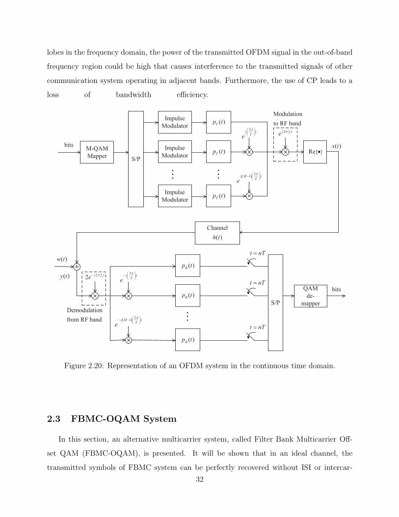
lobes in the frequency domain, the power of the transmitted OFDM signal in the out-of-band

frequency region could be high that causes interference to the transmitted signals of other

communication system operating in adjacent bands. Furthermore, the use of CP leads to a

loss of bandwidth efficiency.

Tp t

j tTe

Tp t

Tp t

j M tTe

h t

w t

Rp t

t nT

Rp t

t nT

Rp t

t nT

x t

y t

cj f te

cj f te j t

Te

j M tTe

Figure 2.20: Representation of an OFDM system in the continuous time domain.

2.3 FBMC-OQAM System

In this section, an alternative multicarrier system, called Filter Bank Multicarrier Off-

set QAM (FBMC-OQAM), is presented. It will be shown that in an ideal channel, the

transmitted symbols of FBMC system can be perfectly recovered without ISI or intercar-

32

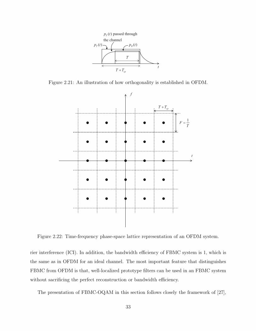
Tp t Rp t

T

cpT Tt

Tp t

Figure 2.21: An illustration of how orthogonality is established in OFDM.

f

t

cpT T

FT

Figure 2.22: Time-frequency phase-space lattice representation of an OFDM system.

rier interference (ICI). In addition, the bandwidth efficiency of FBMC system is 1, which is

the same as in OFDM for an ideal channel. The most important feature that distinguishes

FBMC from OFDM is that, well-localized prototype filters can be used in an FBMC system

without sacrificing the perfect reconstruction or bandwidth efficiency.

The presentation of FBMC-OQAM in this section follows closely the framework of [27],

33

Rs tp t

Tp t

Ijs t

p t

Tp t

p t

Tp t

j M T te

j T te

x t

Rs t

R

Ms t

Ijs t

I

Mjs t

Rs n

Ijs n

Rs n

Ijs n

R

Ms n

I

Mjs n

cj f te

x t

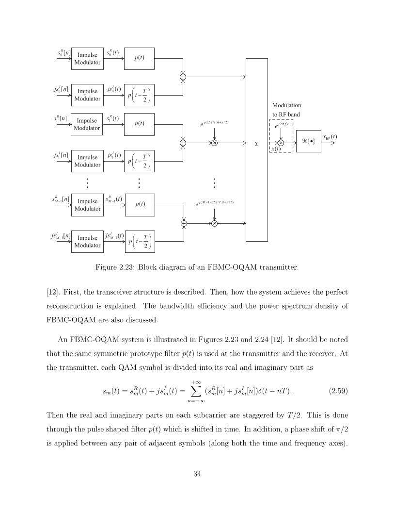
Figure 2.23: Block diagram of an FBMC-OQAM transmitter.

[12]. First, the transceiver structure is described. Then, how the system achieves the perfect

reconstruction is explained. The bandwidth efficiency and the power spectrum density of

FBMC-OQAM are also discussed.

An FBMC-OQAM system is illustrated in Figures 2.23 and 2.24 [12]. It should be noted

that the same symmetric prototype filter p(t) is used at the transmitter and the receiver. At

the transmitter, each QAM symbol is divided into its real and imaginary part as

sm(t) = sRm(t) + jsIm(t) =+∞∑

n=−∞(sRm[n] + jsIm[n])δ(t− nT ). (2.59)

Then the real and imaginary parts on each subcarrier are staggered by T/2. This is done

through the pulse shaped filter p(t) which is shifted in time. In addition, a phase shift of π/2

is applied between any pair of adjacent symbols (along both the time and frequency axes).

34

p t

Tp t

p t

Tp t

p t

Tp t

j T te

j M T te

r t

Rs n

Rs n

R

Ms n

Is n

Is n

I

Ms n

cj f te

r t

t nT

t nT

t nT

t nT

t nT

t nT

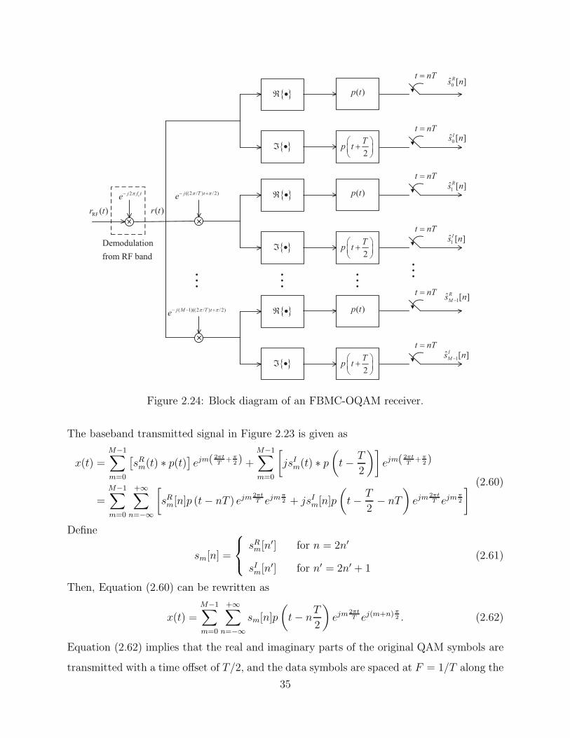
Figure 2.24: Block diagram of an FBMC-OQAM receiver.

The baseband transmitted signal in Figure 2.23 is given as

x(t) =M−1∑

m=0

[sRm(t) ∗ p(t)

]ejm(

2πtT

+π2 ) +

M−1∑

m=0

[

jsIm(t) ∗ p(

t− T

2

)]

ejm(2πtT

+π2 )

=M−1∑

m=0

+∞∑

n=−∞

[

sRm[n]p (t− nT ) ejm2πtT ejm

π2 + jsIm[n]p

(

t− T

2− nT

)

ejm2πtT ejm

π2

] (2.60)

Define

sm[n] =

sRm[n′] for n = 2n′

sIm[n′] for n′ = 2n′ + 1

(2.61)

Then, Equation (2.60) can be rewritten as

x(t) =

M−1∑

m=0

+∞∑

n=−∞sm[n]p

(

t− nT

2

)

ejm2πtT ej(m+n)π

2 . (2.62)

Equation (2.62) implies that the real and imaginary parts of the original QAM symbols are

transmitted with a time offset of T/2, and the data symbols are spaced at F = 1/T along the

35

2

T 3

2

T 2TT

2

T-

T-3

2

T-2T-

1

T

2

T

1

T

-

2

T

-

·

·

·

·

·

·

·

·

·

·

·

·

·

·

·

·

·

·

·

·

·

·

·

·

·

·

·

·

·

·

·

·

·

·

·

·

·

·

·

·

·

·

·

·

·

·

·

·

·

·

·

·

·

·

·

·

·

·

·

·

·

·

·

·

·

·

·

·

·

·

·

·

·

·

·

·

·

·

·

·

·

·

·

·

Figure 2.25: Time frequency phase space for transmission of FBMC-OQAM system.

frequency axis. In addition, the term ej(m+n)π2 indicates the phase offset of π/2 between any

pair of adjacent symbols along the time and frequency axes as illustrated in time-frequency

phase-space lattice representation in Figure 2.25, where the blue dots denote phase shift of

integer factor of π and the orange dots denote phase shift of odd factor of π/2. It is obvious

from the figure that there is one symbol over an area of T/2×F = 1/2, which results in the

density symbol of two. However, notice that the symbol in Figure 2.25 is a real symbol (sRm[n]

or sIm[n]) and it carries one half of the information bits of the original complex QAM symbol

(sm[n]). Thus, one can conclude that FBMC-OQAM achieves the bandwidth efficiency of

one, the same as OFDM system illustrated in Figure 2.22.

Figure 2.24 depicts the receiver of an FBMC-OQAM system. The detected data symbols

at the receiver output are denoted as sRm[n] (or sIm[n]). The filter p(t) should be designed

to have perfect reconstruction, i.e., sRm[n] = sRm[n] when the channel is ideal (there is no

multipath fading and noise). The condition of p(t) for such a perfect recovery is discussed

next.

First, in an FBMC-OQAM system, the prototype filter is designed with an assumption

36

that p(t) is band-limited such that only adjacent subcarrier channels overlap [28]. Thus, one

can ignore possible interference from non-adjacent bands. In that case, there are only three

interference scenarios that may happen:

1. The ISI on each subcarrier, that is, sRm[n] interferences with sRm[n′] for n 6= n′, and

similarly for sIm[n].

2. The cross interference between sRm[n] and sIm[n].

3. ICI among the adjacent subcarrier signals.

To investigate the first and second scenarios, consider the relevant branches from Figure

2.23 and 2.24 that connect sRm[n] and jsIm[n] to sRm[n] and sIm[n]. In an ideal channel, these

branches are illustrated in Figure 2.26. It is noted that the subcarrier modulator ejm(2πtT

+π2 )

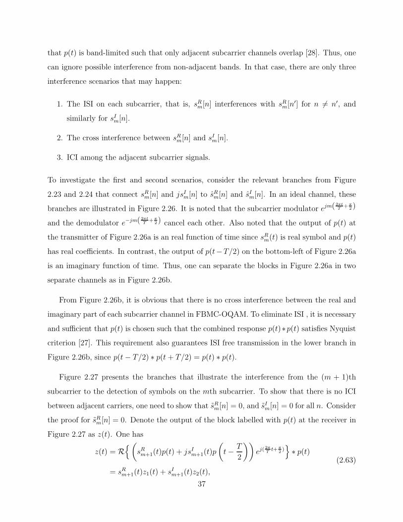
and the demodulator e−jm( 2πtT

+π2 ) cancel each other. Also noted that the output of p(t) at

the transmitter of Figure 2.26a is an real function of time since sRm(t) is real symbol and p(t)

has real coefficients. In contrast, the output of p(t−T/2) on the bottom-left of Figure 2.26a

is an imaginary function of time. Thus, one can separate the blocks in Figure 2.26a in two

separate channels as in Figure 2.26b.

From Figure 2.26b, it is obvious that there is no cross interference between the real and

imaginary part of each subcarrier channel in FBMC-OQAM. To eliminate ISI , it is necessary

and sufficient that p(t) is chosen such that the combined response p(t)∗p(t) satisfies Nyquistcriterion [27]. This requirement also guarantees ISI free transmission in the lower branch in

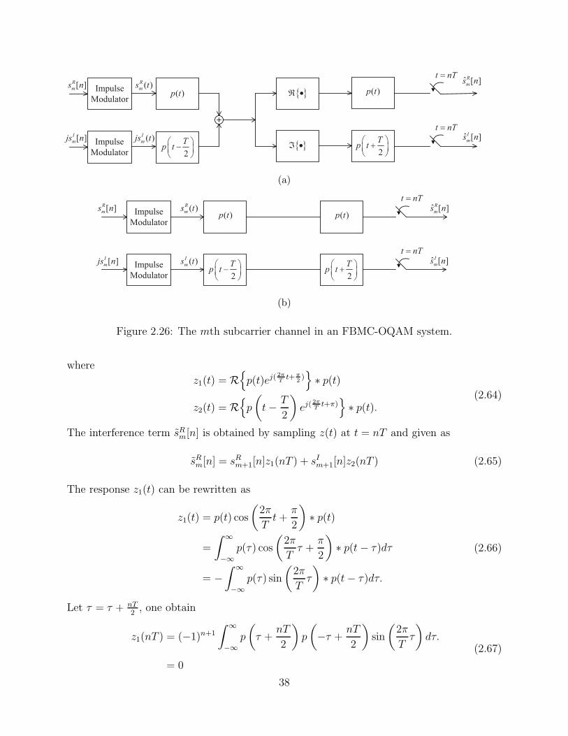
Figure 2.26b, since p(t− T/2) ∗ p(t + T/2) = p(t) ∗ p(t).

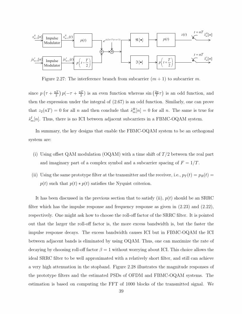
Figure 2.27 presents the branches that illustrate the interference from the (m + 1)th

subcarrier to the detection of symbols on the mth subcarrier. To show that there is no ICI

between adjacent carriers, one need to show that sRm[n] = 0, and sIm[n] = 0 for all n. Consider

the proof for sRm[n] = 0. Denote the output of the block labelled with p(t) at the receiver in

Figure 2.27 as z(t). One has

z(t) = R{(

sRm+1(t)p(t) + jsIm+1(t)p

(

t− T

2

))

ej(2πTt+π

2)}

∗ p(t)

= sRm+1(t)z1(t) + sIm+1(t)z2(t),

(2.63)

37

m

Rs tp t

Tp t

m

Ijs t

p t

Tp t

R

ms n

I

ms n

m

Rs n

m

Ijs n

t nT

t nT

(a)

R

ms tp t

Tp t

I

ms t

p t

Tp t

R

ms n

I

ms n

m

Rs n

m

Ijs n

t nT

t nT

(b)

Figure 2.26: The mth subcarrier channel in an FBMC-OQAM system.

where

z1(t) = R{

p(t)ej(2πT

t+π2)}

∗ p(t)

z2(t) = R{

p

(

t− T

2

)

ej(2πTt+π)}

∗ p(t).(2.64)

The interference term sRm[n] is obtained by sampling z(t) at t = nT and given as

sRm[n] = sRm+1[n]z1(nT ) + sIm+1[n]z2(nT ) (2.65)

The response z1(t) can be rewritten as

z1(t) = p(t) cos

(2π

Tt+

π

2

)

∗ p(t)

=

∫ ∞

−∞p(τ) cos

(2π

Tτ +

π

2

)

∗ p(t− τ)dτ

= −∫ ∞

−∞p(τ) sin

(2π

Tτ

)

∗ p(t− τ)dτ.

(2.66)

Let τ = τ + nT2, one obtain

z1(nT ) = (−1)n+1

∫ ∞

−∞p

(

τ +nT

2

)

p

(

−τ +nT

2

)

sin

(2π

Tτ

)

dτ.

= 0

(2.67)

38

R

ms tp t

Tp t

m

Ijs t

p t

Tp t

R

ms n

I

ms n

j T tem

Rs n

m

Ijs n

z tt nT

t nT

Figure 2.27: The interference branch from subcarrier (m+ 1) to subcarrier m.

since p(τ + nT

2

)p(−τ + nT

2) is an even function whereas sin

(2πTτ)is an odd function, and

then the expression under the integral of (2.67) is an odd function. Similarly, one can prove

that z2(nT ) = 0 for all n and then conclude that sRm[n] = 0 for all n. The same is true for

sIm[n]. Thus, there is no ICI between adjacent subcarriers in a FBMC-OQAM system.

In summary, the key designs that enable the FBMC-OQAM system to be an orthogonal

system are:

(i) Using offset QAM modulation (OQAM) with a time shift of T/2 between the real part

and imaginary part of a complex symbol and a subcarrier spacing of F = 1/T .

(ii) Using the same prototype filter at the transmitter and the receiver, i.e., pT (t) = pR(t) =

p(t) such that p(t) ∗ p(t) satisfies the Nyquist criterion.

It has been discussed in the previous section that to satisfy (ii), p(t) should be an SRRC

filter which has the impulse response and frequency response as given in (2.23) and (2.22),

respectively. One might ask how to choose the roll-off factor of the SRRC filter. It is pointed

out that the larger the roll-off factor is, the more excess bandwidth is, but the faster the

impulse response decays. The excess bandwidth causes ICI but in FBMC-OQAM the ICI

between adjacent bands is eliminated by using OQAM. Thus, one can maximize the rate of

decaying by choosing roll-off factor β = 1 without worrying about ICI. This choice allows the

ideal SRRC filter to be well approximated with a relatively short filter, and still can achieve

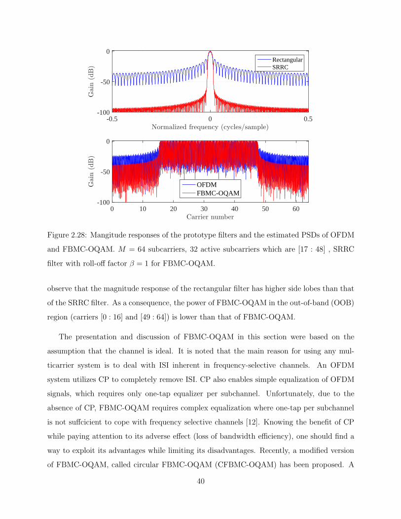
a very high attenuation in the stopband. Figure 2.28 illustrates the magnitude responses of

the prototype filters and the estimated PSDs of OFDM and FBMC-OQAM systems. The

estimation is based on computing the FFT of 1000 blocks of the transmitted signal. We

39

Normalized frequency (cycles/sample)-0.5 0 0.5

Gain

(dB)

-100

-50

0RectangularSRRC

Carrier number0 10 20 30 40 50 60

Gain

(dB)

-100

-50

0

OFDMFBMC-OQAM

Figure 2.28: Mangitude responses of the prototype filters and the estimated PSDs of OFDM

and FBMC-OQAM. M = 64 subcarriers, 32 active subcarriers which are [17 : 48] , SRRC

filter with roll-off factor β = 1 for FBMC-OQAM.

observe that the magnitude response of the rectangular filter has higher side lobes than that

of the SRRC filter. As a consequence, the power of FBMC-OQAM in the out-of-band (OOB)

region (carriers [0 : 16] and [49 : 64]) is lower than that of FBMC-OQAM.

The presentation and discussion of FBMC-OQAM in this section were based on the

assumption that the channel is ideal. It is noted that the main reason for using any mul-

ticarrier system is to deal with ISI inherent in frequency-selective channels. An OFDM

system utilizes CP to completely remove ISI. CP also enables simple equalization of OFDM

signals, which requires only one-tap equalizer per subchannel. Unfortunately, due to the

absence of CP, FBMC-OQAM requires complex equalization where one-tap per subchannel

is not suffcicient to cope with frequency selective channels [12]. Knowing the benefit of CP

while paying attention to its adverse effect (loss of bandwidth efficiency), one should find a

way to exploit its advantages while limiting its disadvantages. Recently, a modified version

of FBMC-OQAM, called circular FBMC-OQAM (CFBMC-OQAM) has been proposed. A

40

CFBMC-OQAM system not only benefits from all good properties of FBMC-OQAM system

but also has the simple equalization like OFDM system due to the use of CP. Details of this

scheme will be presented in the next chapter.

41

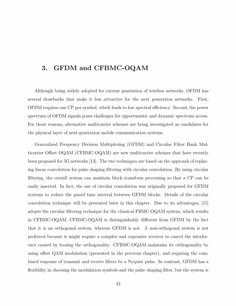
3. GFDM and CFBMC-OQAM

Although being widely adopted for current generation of wireless networks, OFDM has

several drawbacks that make it less attractive for the next generation networks. First,

OFDM requires one CP per symbol, which leads to low spectral efficiency. Second, the power

spectrum of OFDM signals poses challenges for opportunistic and dynamic spectrum access.

For those reasons, alternative multicarrier schemes are being investigated as candidates for

the physical layer of next-generation mobile communication systems.

Generalized Frequency Division Multiplexing (GFDM) and Circular Filter Bank Mul-

ticarrier Offset OQAM (CFBMC-OQAM) are new multicarrier schemes that have recently

been proposed for 5G networks [13]. The two techniques are based on the approach of replac-

ing linear convolution for pulse shaping filtering with circular convolution. By using circular

filtering, the overall system can maintain block transform processing so that a CP can be

easily inserted. In fact, the use of circular convolution was originally proposed for GFDM

systems to reduce the guard time interval between GFDM blocks. Details of the circular

convolution technique will be presented later in this chapter. Due to its advantages, [15]

adopts the circular filtering technique for the classical FBMC-OQAM system, which results

in CFBMC-OQAM. CFBMC-OQAM is distinguishably different from GFDM by the fact

that it is an orthogonal system, whereas GFDM is not. A non-orthogonal system is not

preferred because it might require a complex and expensive receiver to cancel the interfer-

ence caused by loosing the orthogonality. CFBMC-OQAM maintains its orthogonality by

using offset QAM modulation (presented in the previous chapter), and requiring the com-

bined response of transmit and receive filters be a Nyquist pulse. In contrast, GFDM has a

flexibility in choosing the modulation symbols and the pulse shaping filter, but the system is

42

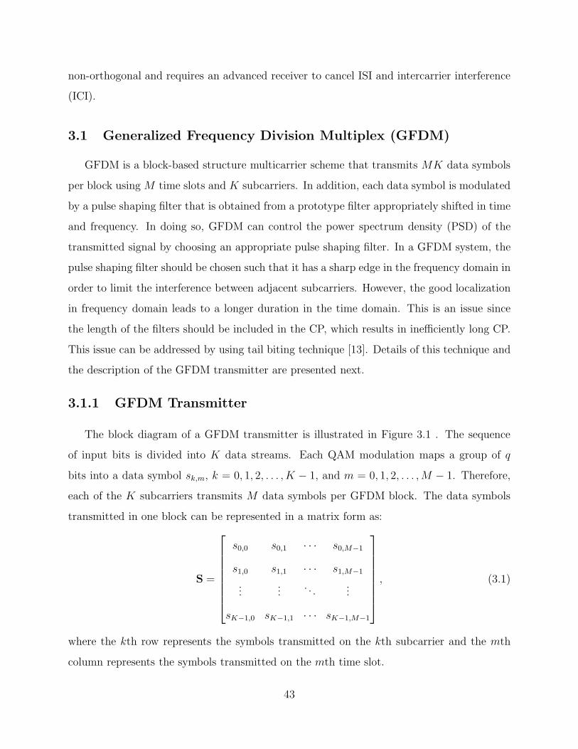
non-orthogonal and requires an advanced receiver to cancel ISI and intercarrier interference

(ICI).

3.1 Generalized Frequency Division Multiplex (GFDM)

GFDM is a block-based structure multicarrier scheme that transmits MK data symbols

per block using M time slots and K subcarriers. In addition, each data symbol is modulated

by a pulse shaping filter that is obtained from a prototype filter appropriately shifted in time

and frequency. In doing so, GFDM can control the power spectrum density (PSD) of the

transmitted signal by choosing an appropriate pulse shaping filter. In a GFDM system, the

pulse shaping filter should be chosen such that it has a sharp edge in the frequency domain in

order to limit the interference between adjacent subcarriers. However, the good localization

in frequency domain leads to a longer duration in the time domain. This is an issue since

the length of the filters should be included in the CP, which results in inefficiently long CP.

This issue can be addressed by using tail biting technique [13]. Details of this technique and

the description of the GFDM transmitter are presented next.

3.1.1 GFDM Transmitter

The block diagram of a GFDM transmitter is illustrated in Figure 3.1 . The sequence

of input bits is divided into K data streams. Each QAM modulation maps a group of q

bits into a data symbol sk,m, k = 0, 1, 2, . . . , K − 1, and m = 0, 1, 2, . . . ,M − 1. Therefore,

each of the K subcarriers transmits M data symbols per GFDM block. The data symbols

transmitted in one block can be represented in a matrix form as:

S =

s0,0 s0,1 · · · s0,M−1

s1,0 s1,1 · · · s1,M−1

......

. . ....

sK−1,0 sK−1,1 · · · sK−1,M−1

, (3.1)

where the kth row represents the symbols transmitted on the kth subcarrier and the mth

column represents the symbols transmitted on the mth time slot.

43

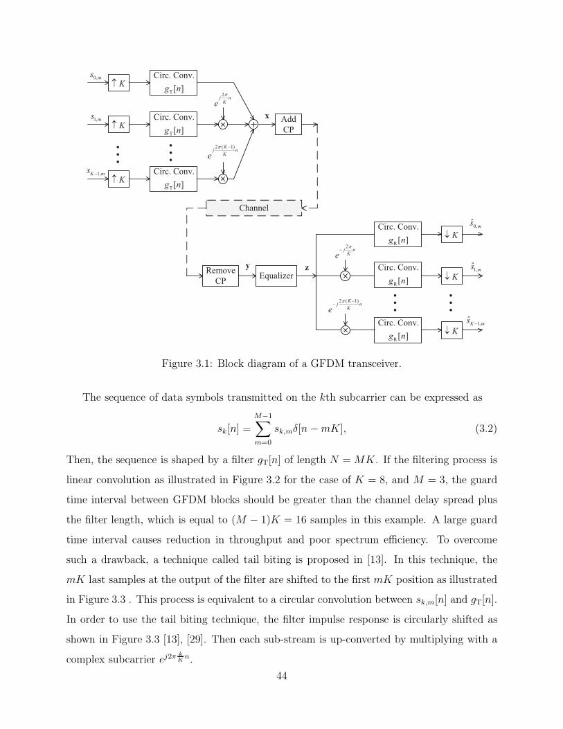
ms

ms

K ms

j nKe

Kj n

Ke

j nKe

Kj n

Ke

K

K

K

K

K

K

ms

ms

K ms

g n

g n

g n

g n

g n

g n

Figure 3.1: Block diagram of a GFDM transceiver.

The sequence of data symbols transmitted on the kth subcarrier can be expressed as

sk[n] =M−1∑

m=0

sk,mδ[n−mK], (3.2)

Then, the sequence is shaped by a filter gT[n] of length N = MK. If the filtering process is

linear convolution as illustrated in Figure 3.2 for the case of K = 8, and M = 3, the guard

time interval between GFDM blocks should be greater than the channel delay spread plus

the filter length, which is equal to (M − 1)K = 16 samples in this example. A large guard

time interval causes reduction in throughput and poor spectrum efficiency. To overcome

such a drawback, a technique called tail biting is proposed in [13]. In this technique, the

mK last samples at the output of the filter are shifted to the first mK position as illustrated

in Figure 3.3 . This process is equivalent to a circular convolution between sk,m[n] and gT[n].

In order to use the tail biting technique, the filter impulse response is circularly shifted as

shown in Figure 3.3 [13], [29]. Then each sub-stream is up-converted by multiplying with a

complex subcarrier ej2πkKn.

44

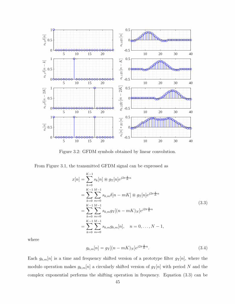
5 10 15 20

s k,0δ[n]

0

0.5

1

10 20 30 40

s k,0g T

[n]

-0.5

0

0.5

5 10 15 20

s k,1δ[n

−k]

0

0.5

1

10 20 30 40

s k,1g T

[n−K]

-0.5

0

0.5

5 10 15 20

s k,2δ[n

−2K

]

0

0.5

1

10 20 30 40

s k,2g T

[n−2K

]

-0.5

0

0.5

5 10 15 20

s k[n]

0

0.5

1

10 20 30 40

s k[n]∗

g T[n]

-0.5

0

0.5

Figure 3.2: GFDM symbols obtained by linear convolution.

From Figure 3.1, the transmitted GFDM signal can be expressed as

x[n] =K−1∑

k=0

sk[n]⊛ gT[n]ej2π k

Kn

=

K−1∑

k=0

M−1∑

m=0

sk,mδ[n−mK]⊛ gT[n]ej2π k

Kn

=

K−1∑

k=0

M−1∑

m=0

sk,mgT[(n−mK)N ]ej2π k

Kn

=K−1∑

k=0

M−1∑

m=0

sk,mgk,m[n], n = 0, . . . , N − 1,

(3.3)

where

gk,m[n] = gT[(n−mK)N ]ej2π k

Kn. (3.4)

Each gk,m[n] is a time and frequency shifted version of a prototype filter gT[n], where the

modulo operation makes gk,m[n] a circularly shifted version of gT[n] with period N and the

complex exponential performs the shifting operation in frequency. Equation (3.3) can be

45

5 10 15 20

s k,0δ[n]

0

0.5

1

5 10 15 20

s k,0g T

[n]

-0.5

0

0.5

5 10 15 20

s k,1δ[n

−K]

0

0.5

1

5 10 15 20s k,1g T

[(n−K) N

]

-0.5

0

0.5

5 10 15 20

s k,2δ[n

−2K

]

0

0.5

1

5 10 15 20s k,2g T

[(n−2K

) N]

-0.5

0

0.5

5 10 15 20

s k[n]

0

0.5

1

5 10 15 20

s k[n]⊗

g T[n]

0

0.5

Figure 3.3: GFDM symbols obtained by circular convolution.

rewritten in a matrix form as:

x = Ad, (3.5)

where x = [x[0], x[1], . . . , x[N − 1]]T, d = [s0,0, s1,0, . . . , sK−1,0, s0,1, s1,1, . . . , sK−1,M−1]T and

A =[

g0,0 . . . gK−1,0 g0,1 . . . gK−1,M−1

]

(3.6)

with gk,m = [gk,m[0], gk,m[1], . . . , gk,m[N − 1]]T.

From Equation (3.3) it is pointed out that each symbol sk,m of a GFDM block is trans-

mitted by gk,m[n]. The set of gk,m[n] for all k and m is not an orthogonal set leading to two

kinds of interference. The intersymbol interference (ISI) between sk,m and sk,m′ for m 6= m′,

and the intercarrier interference (ICI) between sk,m and sk′,m for k 6= k′. The impact of ISI

and ICI on the performance of GFDM depends on which prototype filter is chosen to produce

gTx[n]. The Raised Cosine (RC) and Square Root Raised Cosine (SRRC) filters have been

investigated as prototype filters for GFDM systems in [30]. The analysis show that if RC

46

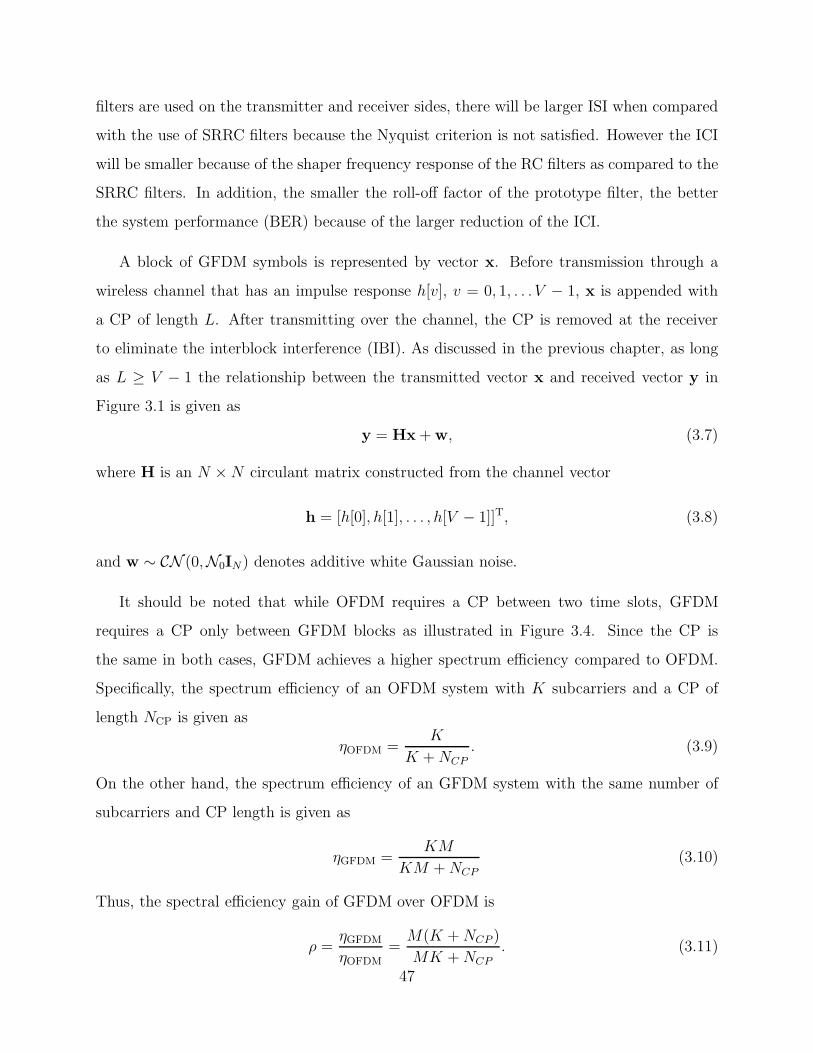
filters are used on the transmitter and receiver sides, there will be larger ISI when compared

with the use of SRRC filters because the Nyquist criterion is not satisfied. However the ICI

will be smaller because of the shaper frequency response of the RC filters as compared to the

SRRC filters. In addition, the smaller the roll-off factor of the prototype filter, the better

the system performance (BER) because of the larger reduction of the ICI.

A block of GFDM symbols is represented by vector x. Before transmission through a

wireless channel that has an impulse response h[v], v = 0, 1, . . . V − 1, x is appended with

a CP of length L. After transmitting over the channel, the CP is removed at the receiver

to eliminate the interblock interference (IBI). As discussed in the previous chapter, as long

as L ≥ V − 1 the relationship between the transmitted vector x and received vector y in

Figure 3.1 is given as

y = Hx+w, (3.7)

where H is an N ×N circulant matrix constructed from the channel vector

h = [h[0], h[1], . . . , h[V − 1]]T, (3.8)

and w ∼ CN (0,N0IN) denotes additive white Gaussian noise.

It should be noted that while OFDM requires a CP between two time slots, GFDM

requires a CP only between GFDM blocks as illustrated in Figure 3.4. Since the CP is

the same in both cases, GFDM achieves a higher spectrum efficiency compared to OFDM.

Specifically, the spectrum efficiency of an OFDM system with K subcarriers and a CP of

length NCP is given as

ηOFDM =K

K +NCP. (3.9)

On the other hand, the spectrum efficiency of an GFDM system with the same number of

subcarriers and CP length is given as

ηGFDM =KM

KM +NCP

(3.10)

Thus, the spectral efficiency gain of GFDM over OFDM is

ρ =ηGFDM

ηOFDM=

M(K +NCP )

MK +NCP. (3.11)

47

s

s

s

s

s

s

s

s

s

s

s

s

s

s

s

s

s

s

s

s

s

s

s

s

s

s

s

s

s

s

s

s

s

s

s

s

s

s

s

s

s

s

s

s

s

s

s

s

s

s

Figure 3.4: Block structures of OFDM and GFDM systems for M = 5 and K = 4.

For example, with K = 64, M = 32, and NCP = 16, the spectrum efficiency gain of GFDM

over OFDM is ρ = 1.25, i.e., 25% increase.

3.1.2 GFDM Receiver

Since H in (3.7) is a circular convolution matrix, the received signal y can be equal-

ized using the zero-forcing equalizer as efficiently used in OFDM. The equalized signal

z = [z[0], z[1], . . . , z[N − 1]]T can be expressed as

z = H−1y

= H−1HAd+H−1w

= Ad+ w

(3.12)

where w = H−1w. After equalization, a GFDM demodulator is applied to reconstruct the

data. In particular, sk,m is obtained by reversing the frequency shift, circular convolving

48

with receive filter gR[n], and downsampling the resulting signal at n = mK according to:

sk,m =(

z[n]e−j2π kKn)

⊛ gR[n]∣∣∣n=mK

=

N−1∑

n=0

z[n]gR[(mK − n)N ]e−j2π k

Kn

=

N−1∑

n=0

z[n]γk,m,

(3.13)

where

γk,m = gR[(mK − n)N ]e−j2π k

Kn. (3.14)

Stacking all demodulated data symbol sk,m into a vector

d = [s0,0, s1,0, . . . , sK−1,0, s0,1, s1,1, . . . , sK−1,M−1]T ,

it then follows from (3.13) and (3.14) that

d = Bz, (3.15)

where

B =[

γ0,0 . . . γK−1,0 γ0,1 . . . γK−1,M−1

]T

(3.16)

with γk,m = [γk,m[0], γk,m[1], . . . , γk,m[N − 1]]T. The demodulated data d depends on the

choice of the receive filter gR[n] through matrix B. There are several demodulation ap-

proaches for GFDM that have been investigated in literature [31]. In the following, two

popular approacheas are reviewed, which are matched filter receiver (MFR) and zero-forcing

receiver (ZFR).

Matched Filter Receiver

To realize the matched filter receiver, gR[n] is chosen to be gR[n] = gT[n] = g[n]. Figure

3.5 illustrates an example of g[n] that has coefficients from a discrete SRRC designed with

M = 3, K = 4, and a roll-off factor β = 0.5. It is noted that the SRRC filter has an

odd number of taps (13 taps). However, to enable circular convolution in GFDM, the

length of g[n] should be N = KM = 12. Thus, g[n] is obtained by removing the last

sample in gSRRC[n] as shown in the center part of Figure 3.5. The lower part of Figure 3.5

49

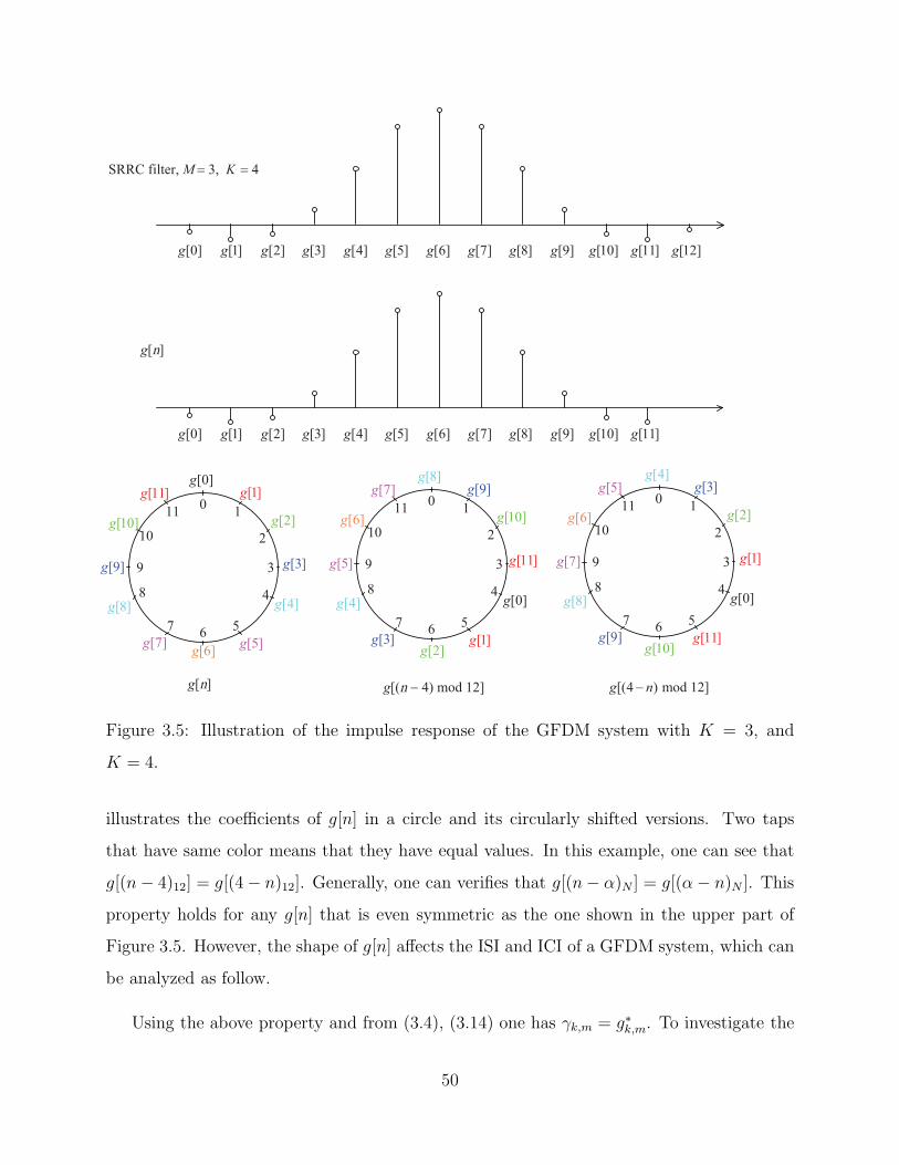
g g g g g g g g g g g g g

g g g g g g g g g g g g

gg

g

g

g

gg

g

g

g

g

gg

g

g

g

gg

g

g

g

g

g

gg

g

g

g

gg

g

g

g

g

g

g

g g g n

M K

g

Figure 3.5: Illustration of the impulse response of the GFDM system with K = 3, and

K = 4.

illustrates the coefficients of g[n] in a circle and its circularly shifted versions. Two taps

that have same color means that they have equal values. In this example, one can see that

g[(n− 4)12] = g[(4− n)12]. Generally, one can verifies that g[(n− α)N ] = g[(α− n)N ]. This

property holds for any g[n] that is even symmetric as the one shown in the upper part of

Figure 3.5. However, the shape of g[n] affects the ISI and ICI of a GFDM system, which can

be analyzed as follow.

Using the above property and from (3.4), (3.14) one has γk,m = g∗k,m. To investigate the

50

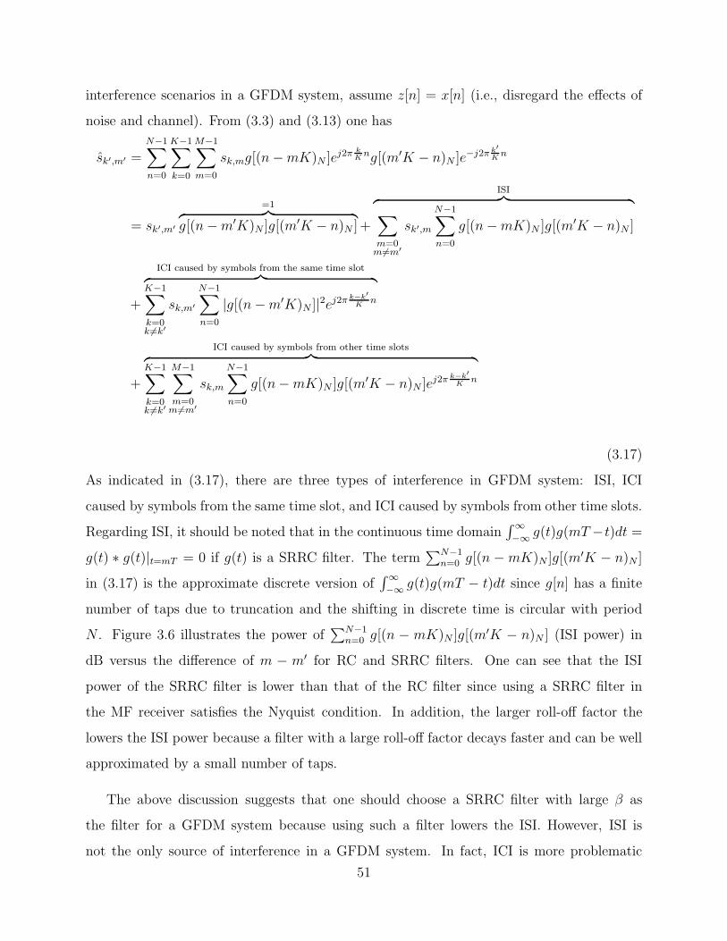
interference scenarios in a GFDM system, assume z[n] = x[n] (i.e., disregard the effects of

noise and channel). From (3.3) and (3.13) one has

sk′,m′ =

N−1∑

n=0

K−1∑

k=0

M−1∑

m=0

sk,mg[(n−mK)N ]ej2π k

Kng[(m′K − n)N ]e

−j2π k′

Kn

= sk′,m′

=1︷︸︸︷

g[(n−m′K)N ]g[(m′K − n)N ] +

ISI︷︸︸︷

∑

m=0m6=m′

sk′,m

N−1∑

n=0

g[(n−mK)N ]g[(m′K − n)N ]

+

ICI caused by symbols from the same time slot︷︸︸︷K−1∑

k=0k 6=k′

sk,m′

N−1∑

n=0

|g[(n−m′K)N ]|2ej2πk−k′

Kn

+

ICI caused by symbols from other time slots︷︸︸︷K−1∑

k=0k 6=k′

M−1∑

m=0m6=m′

sk,m

N−1∑

n=0

g[(n−mK)N ]g[(m′K − n)N ]e

j2π k−k′

Kn

(3.17)

As indicated in (3.17), there are three types of interference in GFDM system: ISI, ICI

caused by symbols from the same time slot, and ICI caused by symbols from other time slots.

Regarding ISI, it should be noted that in the continuous time domain∫∞−∞ g(t)g(mT−t)dt =

g(t) ∗ g(t)|t=mT = 0 if g(t) is a SRRC filter. The term∑N−1

n=0 g[(n − mK)N ]g[(m′K − n)N ]

in (3.17) is the approximate discrete version of∫∞−∞ g(t)g(mT − t)dt since g[n] has a finite

number of taps due to truncation and the shifting in discrete time is circular with period

N . Figure 3.6 illustrates the power of∑N−1

n=0 g[(n − mK)N ]g[(m′K − n)N ] (ISI power) in

dB versus the difference of m − m′ for RC and SRRC filters. One can see that the ISI

power of the SRRC filter is lower than that of the RC filter since using a SRRC filter in

the MF receiver satisfies the Nyquist condition. In addition, the larger roll-off factor the

lowers the ISI power because a filter with a large roll-off factor decays faster and can be well

approximated by a small number of taps.

The above discussion suggests that one should choose a SRRC filter with large β as

the filter for a GFDM system because using such a filter lowers the ISI. However, ISI is

not the only source of interference in a GFDM system. In fact, ICI is more problematic

51

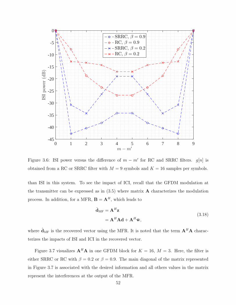
m−m′0 1 2 3 4 5 6 7 8 9

ISIpow

er(dB)

-45

-40

-35

-30

-25

-20

-15

-10

-5

0SRRC, β = 0.9RC, β = 0.9SRRC, β = 0.2RC, β = 0.2

Figure 3.6: ISI power versus the difference of m − m′ for RC and SRRC filters. g[n] is

obtained from a RC or SRRC filter with M = 9 symbols and K = 16 samples per symbols.

than ISI in this system. To see the impact of ICI, recall that the GFDM modulation at

the transmitter can be expressed as in (3.5) where matrix A characterizes the modulation

process. In addition, for a MFR, B = AH , which leads to

dMF = AHz

= AHAd+AHw,(3.18)

where dMF is the recovered vector using the MFR. It is noted that the term AHA charac-

terizes the impacts of ISI and ICI in the recovered vector.

Figure 3.7 visualizes AHA in one GFDM block for K = 16, M = 3. Here, the filter is

either SRRC or RC with β = 0.2 or β = 0.9. The main diagonal of the matrix represented

in Figure 3.7 is associated with the desired information and all others values in the matrix

represent the interferences at the output of the MFR.

52

carrier number10 20 30 40

carriernumber

10

20

30

40

-100

-80

-60

-40

-20

(a) SRRC, β = 0.9, SIR = −0.256 dB


carriernumber

10

20

30

40

-100

-80

-60

-40

-20

(b) RC, β = 0.9, SIR = 0.185 dB


carriernumber

10

20

30

40

-70

-60

-50

-40

-30

-20

-10

(c) SRRC, β = 0.2, SIR = 3.099 dB


carriernumber

10

20

30

40-70

-60

-50

-40

-30

-20

-10

(d) RC, β = 0.2, SIR = 3.723 dB

Figure 3.7: Interference patterns of a GFDM system with M = 3, and K = 16.

From Figure 3.7, one can see that the ICI caused by adjacent subcarriers is prominent

and significantly larger than the one caused by non-adjacent subcarriers. In addition, filters

with small β experience lower ICI than those with large β. This is due to the fact that the

frequency responses of the SRRC and RC filters expand to the adjacent band, and the larger

β, the more expansion. Figure 3.7 also shows that SRRC filters have lower ISI than RC

filters, but RC filters have lower ICI than SRRC filters. The average signal-to-interference

ratio (SIR) of the four cases are also shown in Figure 3.7. Observe that case (a), which uses

a SRRC filter with large β, results in the smallest ISI. However, the large ICI outweights

the benefit of low ISI. As such this case has the lowest SIR. Still using a SRRC filter but

53

with a smaller β, one can reduce the ICI and thus increase the SIR significantly as in case

(c). Consider using a RC filter, one can make a tradeoff between ISI and ICI. For example,

in case d), which uses a RC filter with small β, the system enjoys the largest SIR. Thus,

this case might be a good choice for a GFDM system that is implemented with the matched

filter receiver.

Zero-forcing Receiver

From (3.15), choosing B = A−1 leads to a zero-forcing receiver. This gives

dZF = Bz

= A−1H−1y

= A−1H−1 (HAd+w)

= d+A−1H−1w,

(3.19)

where dZF is the recovered vector using the zero-forcing approach. Consider the performance

of the zero-forcing receiver over an AWGN channel, i.e., H = I. The nth element of dZF can

be expressed as

dZF,n = dn +N−1∑

n′=0

[A−1

]

n,n′wn n = 0, 1, . . . , N − 1 (3.20)

where wn ∼ CN (0,N0). Since w ∼ CN (0,N0I), the variables wn, n = 0, 1, . . . , N − 1 are

independent identically distributed (iid). Denote wn =∑N−1

n′=0 [A−1]n,n′ wn. The variance of

wn is given as

var[wn] =

N−1∑

n′=0

∣∣∣

[A−1

]

n,n′

∣∣∣

2

N0. (3.21)

One can verify that var[wn] is equal for every n. Equation (3.20) can be rewritten as

dZF,n = dn + wn, (3.22)

where wn ∼ CN (0, ξN0), and ξ =∑N−1

n′=0

∣∣∣[A−1]n,n′

∣∣∣

2

. Equation (3.22) shows that the zero-

forcing receiver is able to completely remove the ICI resulted from the non-orthogonality

between the subcarriers. However, this method enhances the noise power in the demodulated

symbols because ξ > 1. Compare Equation (3.22) with the demodulated symbols of an

OFDM system in Equation (2.49), it is expected that the BER curve of a GFDM system has

54

the same slope as the one of an OFDM system. However, the former experiences a power

loss due to the noise enhancement factor ξ.

3.1.3 Efficient Implementation of GFDM

In this part, an efficient implementation for a GFDM system is presented. Then imple-

mentation complexity of different transmitter approaches is compared in term of complex

valued multiplications.

The transmitted GFDM signal in (3.3) can be reformulated as:

x[n] =

M−1∑

m=0

g[(n−mK)N ]

K−1∑

k=0

sk,mej2π k

Kn. (3.23)

Notice that the term∑K−1

k=0 sk,mej2π k

Kn for n = 0, 1, . . . , K−1 is the K-point Inverse Discrete

Fourier Transform (IDFT) of sm = [s0,m, . . . , sK−1,m]T, which is expressed as FH

Ksm, where

F is the K-point Fourier Transform matrix. In addition, the sequence obtained from the

IDFT is periodic with period K. Thus, for n = 0, . . . , N − 1 (N = MK),∑K−1

k=0 sk,mej2π k

Kn

can be obtained by concatenating FHKsm M times, which is represented as RFH

Ksm where

R = [IK , . . . , IK ]T is the repetition matrix.

Multiplication with g[(n − mK)N ] can be expressed by the matrix Gm = diag(Φmg)

where g = [g[0], . . . , g[N − 1]]T, and Φm is an N × N circulant matrix whose first column

has only one non zero value, which is the mKth element. The matrix Gm circular shifting

g[n] according to time slot m.

Using the above matrix notation, one can rewrite (3.23) as

x =

M−1∑

m=0

GmRFHKsm. (3.24)

An example of (3.24) for K = 3, and M = 2 is illustrated in Figure 3.8. Note that in Figure

3.9, the coefficients gn,m, cn,m is the nth element of Φmg, GmRFHKsm, respectively.

The signal x is added a cyclic prefix and then transmitted through a channel with the

input/output relationship expressed in (3.7). Then, the received signal is demodulated as

sm = FRTGmSy, (3.25)

55

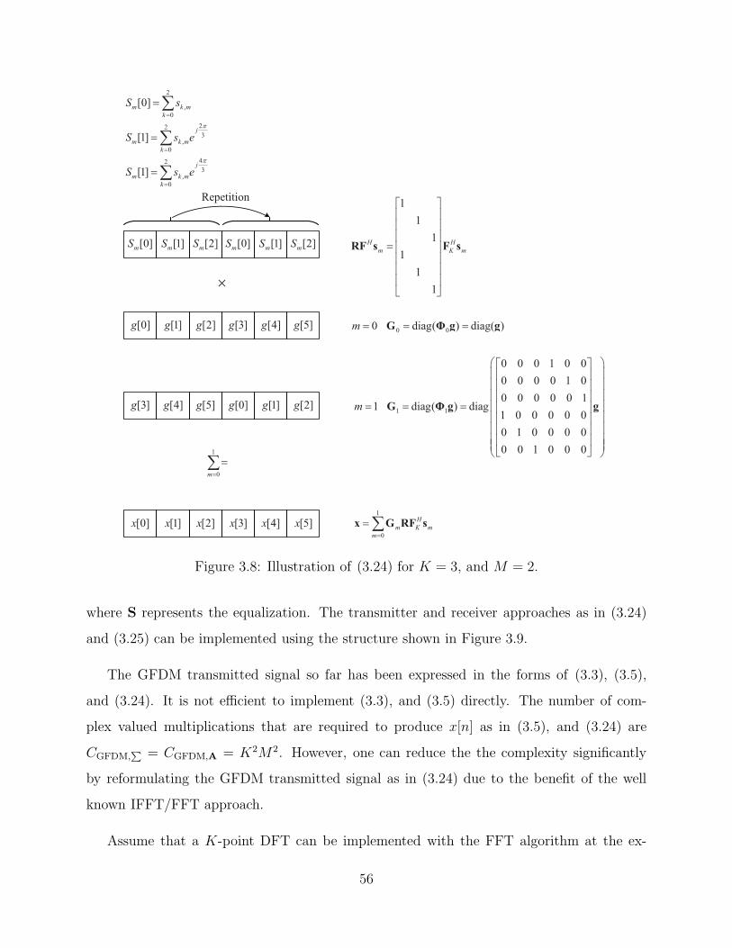
mS mS mS mS mS mS

m k m

k

j

m k m

k

j

m k m

k

S s

S s e

S s e

g g g g g g

g g g g g g

x x x x x x

m

H H

m K m

m

m

H

m K m

m

Figure 3.8: Illustration of (3.24) for K = 3, and M = 2.

where S represents the equalization. The transmitter and receiver approaches as in (3.24)

and (3.25) can be implemented using the structure shown in Figure 3.9.

The GFDM transmitted signal so far has been expressed in the forms of (3.3), (3.5),

and (3.24). It is not efficient to implement (3.3), and (3.5) directly. The number of com-

plex valued multiplications that are required to produce x[n] as in (3.5), and (3.24) are

CGFDM,∑ = CGFDM,A = K2M2. However, one can reduce the the complexity significantly

by reformulating the GFDM transmitted signal as in (3.24) due to the benefit of the well

known IFFT/FFT approach.

Assume that a K-point DFT can be implemented with the FFT algorithm at the ex-

56

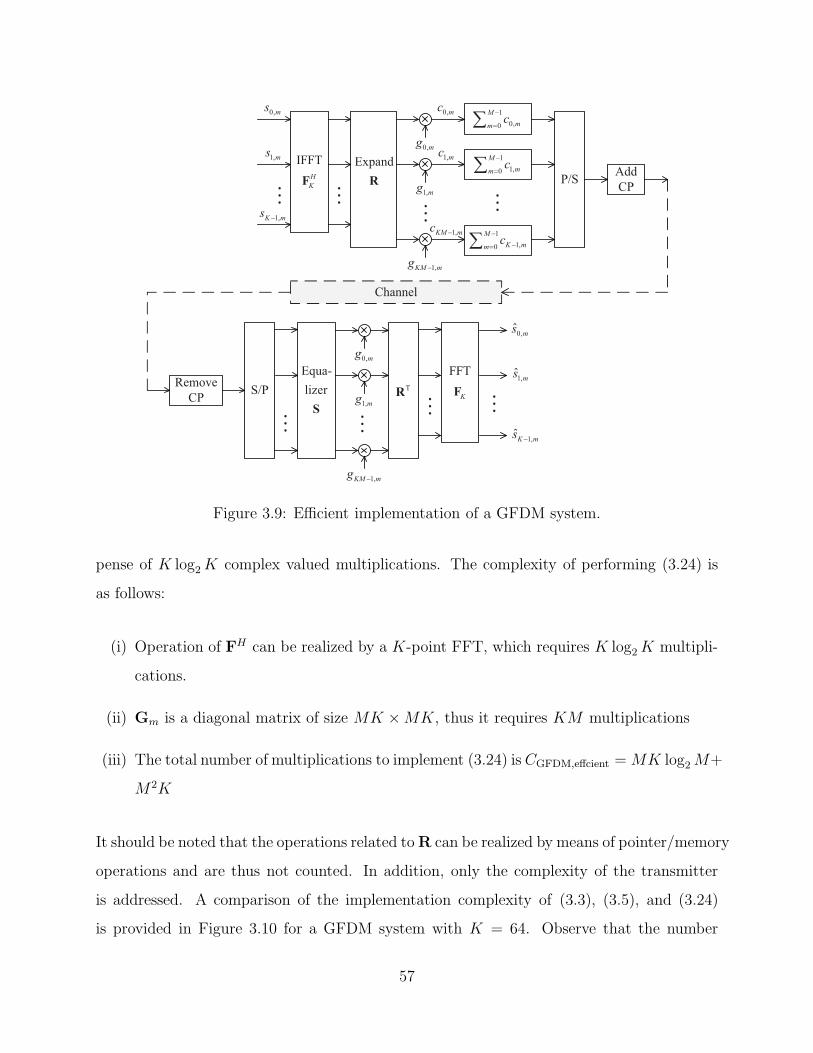
ms

H

K

M

m mc

ms

K ms

mg

mc

mg

mc

KM mg

KM mc

M

m mc

M

m K mc

mg

mg

KM mg

K

ms

ms

K ms

Figure 3.9: Efficient implementation of a GFDM system.

pense of K log2K complex valued multiplications. The complexity of performing (3.24) is

as follows:

(i) Operation of FH can be realized by a K-point FFT, which requires K log2K multipli-

cations.

(ii) Gm is a diagonal matrix of size MK ×MK, thus it requires KM multiplications

(iii) The total number of multiplications to implement (3.24) is CGFDM,effcient = MK log2M+

M2K

It should be noted that the operations related toR can be realized by means of pointer/memory

operations and are thus not counted. In addition, only the complexity of the transmitter

is addressed. A comparison of the implementation complexity of (3.3), (3.5), and (3.24)

is provided in Figure 3.10 for a GFDM system with K = 64. Observe that the number

57

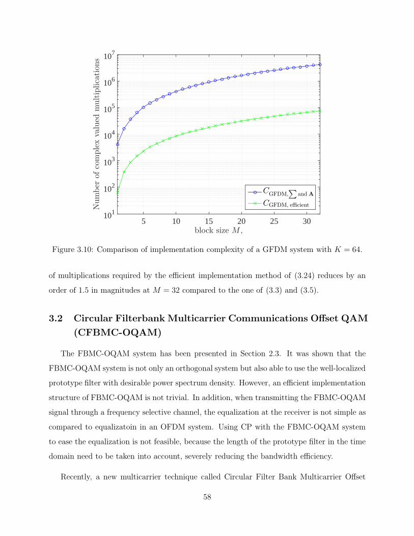
block size M ,5 10 15 20 25 30

Number

ofcomplexvalued

multiplications

101

102

103

104

105

106

107

CGFDM,∑

and A

CGFDM, efficient

Figure 3.10: Comparison of implementation complexity of a GFDM system with K = 64.

of multiplications required by the efficient implementation method of (3.24) reduces by an

order of 1.5 in magnitudes at M = 32 compared to the one of (3.3) and (3.5).

3.2 Circular Filterbank Multicarrier Communications Offset QAM

(CFBMC-OQAM)

The FBMC-OQAM system has been presented in Section 2.3. It was shown that the

FBMC-OQAM system is not only an orthogonal system but also able to use the well-localized

prototype filter with desirable power spectrum density. However, an efficient implementation

structure of FBMC-OQAM is not trivial. In addition, when transmitting the FBMC-OQAM

signal through a frequency selective channel, the equalization at the receiver is not simple as

compared to equalizatoin in an OFDM system. Using CP with the FBMC-OQAM system

to ease the equalization is not feasible, because the length of the prototype filter in the time

domain need to be taken into account, severely reducing the bandwidth efficiency.

Recently, a new multicarrier technique called Circular Filter Bank Multicarrier Offset

58

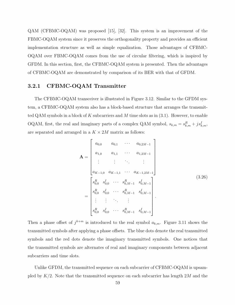
QAM (CFBMC-OQAM) was proposed [15], [32]. This system is an improvement of the

FBMC-OQAM system since it preserves the orthogonality property and provides an efficient

implementation structure as well as simple equalization. Those advantages of CFBMC-

OQAM over FBMC-OQAM comes from the use of circular filtering, which is inspired by

GFDM. In this section, first, the CFBMC-OQAM system is presented. Then the advantages

of CFBMC-OQAM are demonstrated by comparison of its BER with that of GFDM.

3.2.1 CFBMC-OQAM Transmitter

The CFBMC-OQAM transceiver is illustrated in Figure 3.12. Similar to the GFDM sys-

tem, a CFBMC-OQAM system also has a block-based structure that arranges the transmit-

ted QAM symbols in a block ofK subcarriers andM time slots as in (3.1). However, to enable

OQAM, first, the real and imaginary parts of a complex QAM symbol, sk,m = sRk,m + jsIk,m,

are separated and arranged in a K × 2M matrix as follows:

A =

a0,0 a0,1 · · · a0,2M−1

a1,0 a1,1 · · · a1,2M−1

......

. . ....

aK−1,0 aK−1,1 · · · aK−1,2M−1

=

sR0,0 sI0,0 · · · sR0,M−1 sI0,M−1

sR0,0 sI0,0 · · · sR0,M−1 sI0,M−1

......

. . ....

sR0,0 sI0,0 · · · sR0,M−1 sI0,M−1

.

(3.26)

Then a phase offset of jk+m is introduced to the real symbol ak,m. Figure 3.11 shows the

transmitted symbols after applying a phase offsets. The blue dots denote the real transmitted

symbols and the red dots denote the imaginary transmitted symbols. One notices that

the transmitted symbols are alternates of real and imaginary components between adjacent

subcarriers and time slots.

Unlike GFDM, the transmitted sequence on each subcarrier of CFBMC-OQAM is upsam-

pled by K/2. Note that the transmitted sequence on each subcarrier has length 2M and the

59

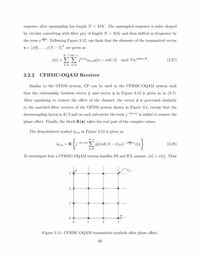
sequence after upsampling has length N = MK. The upsampled sequence is pulse shaped

by circular convolving with filter g[n] of length N = MK and then shifted in frequency by

the term ej2πK

k. Following Figure 3.12, one finds that the elements of the transmitted vector

x = [x[0], . . . , x[N − 1]]T are given as

x[n] =K−1∑

k=0

2M−1∑

m=0

jk+mak,mg[(n−mK/2) mod N ]ej2πkn/K . (3.27)

3.2.2 CFBMC-OQAM Receiver

Similar to the GFDM system, CP can be used in the CFBMC-OQAM system such

that the relationship between vector y and vector x in Figure 3.12 is given as in (3.7).

After equalizing to remove the effect of the channel, the vector z is processed similarly

to the matched filter receiver of the GFDM system shown in Figure 3.1, except that the

downsampling factor is K/2 and on each subcarrier the term j−(k+m) is added to remove the

phase offset. Finally, the block R{•} takes the real part of the complex values.

The demodulated symbol ak,m in Figure 3.12 is given as

ak,m = R

{

j−(k+m)N−1∑

n=0

g[(mK/2− n)N ]e−j 2πk

Knz[n]

}

(3.28)

To investigate how a CFBMC-OQAM system handles ISI and ICI, assume z[n] = x[n]. Then

k m

k mj a

m

k

Figure 3.11: CFBMC-OQAM transmitted symbols after phase offset.

60

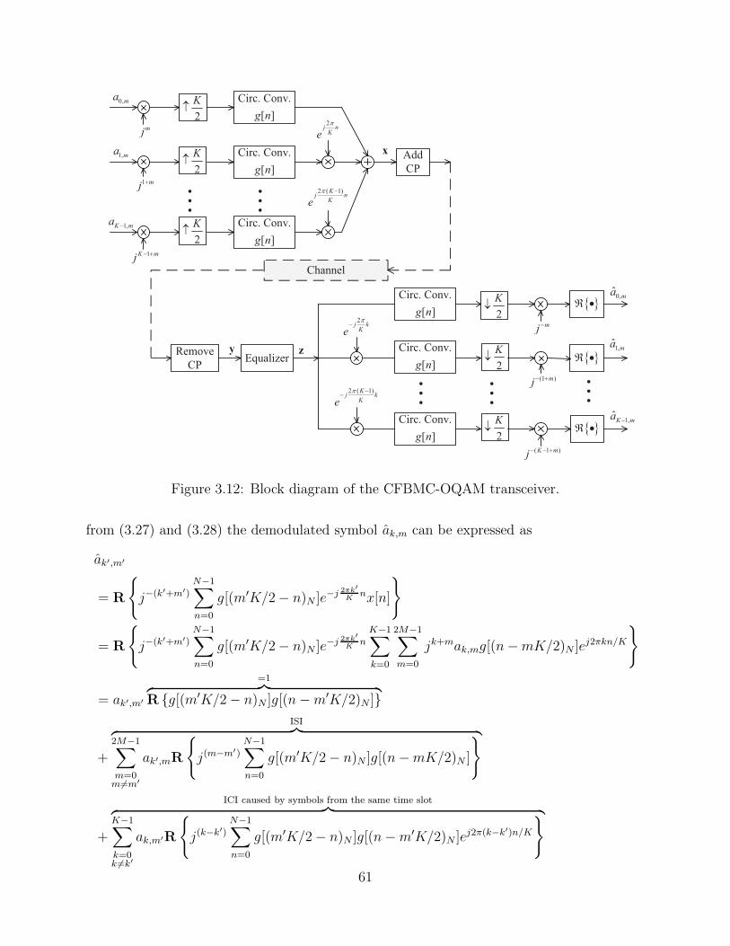
ma

ma

K ma

j nKe

Kj n

Ke

j kKe

Kj k

Ke

K

K

ma

ma

K ma

g n

g n

g n

g n

g n

g n

mj

mj

K mj

mj

mj

K mj

K

K

K

K

Figure 3.12: Block diagram of the CFBMC-OQAM transceiver.

from (3.27) and (3.28) the demodulated symbol ak,m can be expressed as

ak′,m′

= R

{

j−(k′+m′)

N−1∑

n=0

g[(m′K/2− n)N ]e−j 2πk′

Knx[n]

}

= R

{

j−(k′+m′)N−1∑

n=0

g[(m′K/2− n)N ]e−j 2πk′

KnK−1∑

k=0

2M−1∑

m=0

jk+mak,mg[(n−mK/2)N ]ej2πkn/K

}

= ak′,m′

=1︷︸︸︷

R {g[(m′K/2− n)N ]g[(n−m′K/2)N ]}

+

ISI︷︸︸︷2M−1∑

m=0m6=m′

ak′,mR

{

j(m−m′)

N−1∑

n=0

g[(m′K/2− n)N ]g[(n−mK/2)N ]

}

+

ICI caused by symbols from the same time slot︷︸︸︷K−1∑

k=0k 6=k′

ak,m′R

{

j(k−k′)

N−1∑

n=0

g[(m′K/2− n)N ]g[(n−m′K/2)N ]ej2π(k−k′)n/K

}

61

+

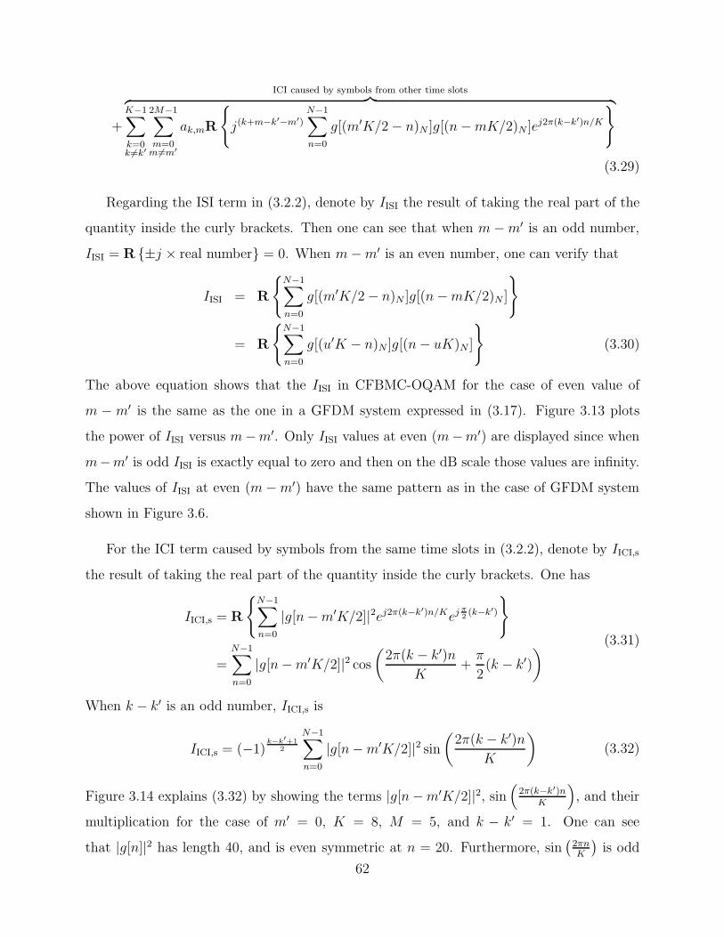
ICI caused by symbols from other time slots︷︸︸︷K−1∑

k=0k 6=k′

2M−1∑

m=0m6=m′

ak,mR

{

j(k+m−k′−m′)

N−1∑

n=0

g[(m′K/2− n)N ]g[(n−mK/2)N ]ej2π(k−k′)n/K

}

(3.29)

Regarding the ISI term in (3.2.2), denote by IISI the result of taking the real part of the

quantity inside the curly brackets. Then one can see that when m −m′ is an odd number,

IISI = R {±j × real number} = 0. When m−m′ is an even number, one can verify that

IISI = R

{N−1∑

n=0

g[(m′K/2− n)N ]g[(n−mK/2)N ]

}

= R

{N−1∑

n=0

g[(u′K − n)N ]g[(n− uK)N ]

}

(3.30)

The above equation shows that the IISI in CFBMC-OQAM for the case of even value of

m − m′ is the same as the one in a GFDM system expressed in (3.17). Figure 3.13 plots

the power of IISI versus m−m′. Only IISI values at even (m−m′) are displayed since when

m−m′ is odd IISI is exactly equal to zero and then on the dB scale those values are infinity.

The values of IISI at even (m−m′) have the same pattern as in the case of GFDM system

shown in Figure 3.6.

For the ICI term caused by symbols from the same time slots in (3.2.2), denote by IICI,s

the result of taking the real part of the quantity inside the curly brackets. One has

IICI,s = R

{N−1∑

n=0

|g[n−m′K/2]|2ej2π(k−k′)n/Kejπ2(k−k′)

}

=N−1∑

n=0

|g[n−m′K/2]|2 cos(2π(k − k′)n

K+

π

2(k − k′)

) (3.31)

When k − k′ is an odd number, IICI,s is

IICI,s = (−1)k−k′+1

2

N−1∑

n=0

|g[n−m′K/2]|2 sin(2π(k − k′)n

K

)

(3.32)

Figure 3.14 explains (3.32) by showing the terms |g[n−m′K/2]|2, sin(

2π(k−k′)nK

)

, and their

multiplication for the case of m′ = 0, K = 8, M = 5, and k − k′ = 1. One can see

that |g[n]|2 has length 40, and is even symmetric at n = 20. Furthermore, sin(2πnK

)is odd

62

m−m′0 2 4 6 8 10 12 14 16 18

ISIpow

er(dB)

-45

-40

-35

-30

-25

-20

-15

-10

-5

0

SRRC, β = 0.9

Figure 3.13: ISI power versus the difference of m−m′, CFBMC-OQAM with SRRC, β = 0.9,

K = 16, and M = 9.

symmetric at n = 20. Thus, their multiplication is odd symmetric at n = 20 and then

−∑N−1n=0 |g[n]|2 sin

(2πnK

)= 0. For other values of m′, |g[n − m′K/2]|2 is a circular shift of

|g[n]|2 then it is circular even symmetric at n = (20 + m′K/2)N . Meanwhile, for any odd

value of k − k′, sin(

2π(k−k′)nK

)

is circular odd symmetric at any n which is a multiple of

K/2. Therefore (3.32) holds true for any m′ and odd value of k − k′. Figure 3.15 illustrates

another example where m′ = 3 and k − k′ = 3.

The above discussion proves that ICI from adjacent subcarriers (k− k′ = 1) in CFBMC-

OQAM system can be eliminated successfully. Furthermore, it can be shown that the ICI

from non-adjacent subcarriers that satisfies k − k′ = 2u + 1 can also be eliminated. Next,

evaluate (3.31) for the case when k − k′ = 2u. One can verify that

IICI,s = (−1)k−k′

2

N−1∑

n=0

|g[n−m′K/2]|2 cos(2π(k − k′)n

K

)

(3.33)

63

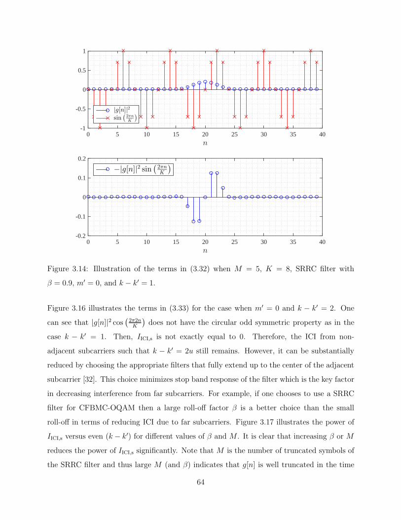
n0 5 10 15 20 25 30 35 40

-1

-0.5

0

0.5

1

|g[n]|2

sin(

2πnK

)

n0 5 10 15 20 25 30 35 40

-0.2

-0.1

0

0.1

0.2

−|g[n]|2 sin(

2πnK

)

Figure 3.14: Illustration of the terms in (3.32) when M = 5, K = 8, SRRC filter with

β = 0.9, m′ = 0, and k − k′ = 1.

Figure 3.16 illustrates the terms in (3.33) for the case when m′ = 0 and k − k′ = 2. One

can see that |g[n]|2 cos(2π2nK

)does not have the circular odd symmetric property as in the

case k − k′ = 1. Then, IICI,s is not exactly equal to 0. Therefore, the ICI from non-

adjacent subcarriers such that k − k′ = 2u still remains. However, it can be substantially

reduced by choosing the appropriate filters that fully extend up to the center of the adjacent

subcarrier [32]. This choice minimizes stop band response of the filter which is the key factor

in decreasing interference from far subcarriers. For example, if one chooses to use a SRRC

filter for CFBMC-OQAM then a large roll-off factor β is a better choice than the small

roll-off in terms of reducing ICI due to far subcarriers. Figure 3.17 illustrates the power of

IICI,s versus even (k − k′) for different values of β and M . It is clear that increasing β or M

reduces the power of IICI,s significantly. Note that M is the number of truncated symbols of

the SRRC filter and thus large M (and β) indicates that g[n] is well truncated in the time

64

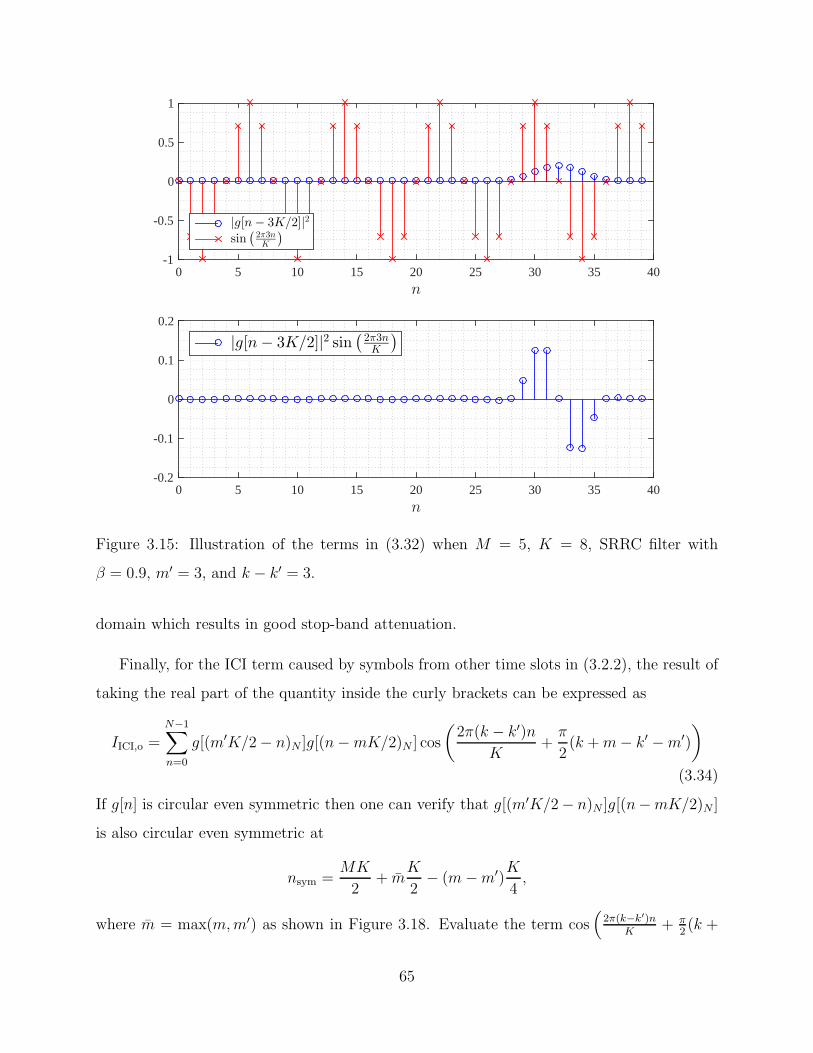
n0 5 10 15 20 25 30 35 40

-1

-0.5

0

0.5

1

|g[n− 3K/2]|2

sin(

2π3nK

)

n0 5 10 15 20 25 30 35 40

-0.2

-0.1

0

0.1

0.2

|g[n− 3K/2]|2 sin(

2π3nK

)


β = 0.9, m′ = 3, and k − k′ = 3.

domain which results in good stop-band attenuation.

Finally, for the ICI term caused by symbols from other time slots in (3.2.2), the result of

taking the real part of the quantity inside the curly brackets can be expressed as

IICI,o =

N−1∑

n=0

g[(m′K/2− n)N ]g[(n−mK/2)N ] cos

(2π(k − k′)n

K+

π

2(k +m− k′ −m′)

)

(3.34)

If g[n] is circular even symmetric then one can verify that g[(m′K/2− n)N ]g[(n−mK/2)N ]

is also circular even symmetric at

nsym =MK

2+ m

K

2− (m−m′)

K

4,

where m = max(m,m′) as shown in Figure 3.18. Evaluate the term cos(

2π(k−k′)nK

+ π2(k +

65

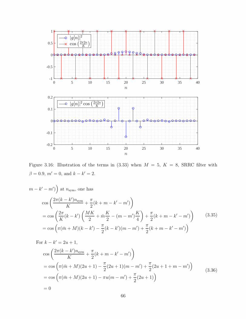
n0 5 10 15 20 25 30 35 40

-1

-0.5

0

0.5

1

|g[n]|2

cos(

2π2nK

)

n0 5 10 15 20 25 30 35 40

-0.2

-0.1

0

0.1

0.2

|g[n]|2 cos(

2π2nK

)


β = 0.9, m′ = 0, and k − k′ = 2.

m− k′ −m′))

at nsym, one has

cos

(2π(k − k′)nsym

K+

π

2(k +m− k′ −m′)

)

= cos

(2π

K(k − k′)

(MK

2+ m

K

2− (m−m′)

K

4

)

+π

2(k +m− k′ −m′)

)

= cos(

π(m+M)(k − k′)− π

2(k − k′)(m−m′) +

π

2(k +m− k′ −m′)

)

(3.35)

For k − k′ = 2u+ 1,

cos


K+

π

2(k +m− k′ −m′)

)

= cos(

π(m+M)(2u+ 1)− π

2(2u+ 1)(m−m′) +

π

2(2u+ 1 +m−m′)

)

= cos(

π(m+M)(2u+ 1)− πu(m−m′) +π

2(2u+ 1)

)

= 0

(3.36)

66

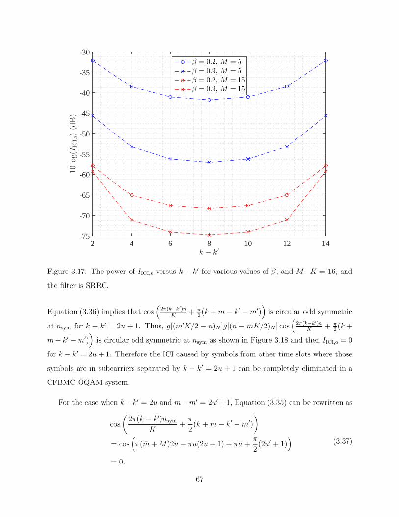
k − k′2 4 6 8 10 12 14

10log(I

ICI,s)

(dB)

-75

-70

-65

-60

-55

-50

-45

-40

-35

-30β = 0.2, M = 5β = 0.9, M = 5β = 0.2, M = 15β = 0.9, M = 15

Figure 3.17: The power of IICI,s versus k − k′ for various values of β, and M . K = 16, and

the filter is SRRC.

Equation (3.36) implies that cos(

2π(k−k′)nK

+ π2(k +m− k′ −m′)

)

is circular odd symmetric

at nsym for k − k′ = 2u + 1. Thus, g[(m′K/2 − n)N ]g[(n−mK/2)N ] cos(

2π(k−k′)nK

+ π2(k +

m− k′ −m′))

is circular odd symmetric at nsym as shown in Figure 3.18 and then IICI,o = 0

for k − k′ = 2u+ 1. Therefore the ICI caused by symbols from other time slots where those

symbols are in subcarriers separated by k − k′ = 2u + 1 can be completely eliminated in a

CFBMC-OQAM system.

For the case when k−k′ = 2u and m−m′ = 2u′+1, Equation (3.35) can be rewritten as

cos


K+

π

2(k +m− k′ −m′)

)

= cos(

π(m+M)2u− πu(2u+ 1) + πu+π

2(2u′ + 1)

)

= 0.

(3.37)

67

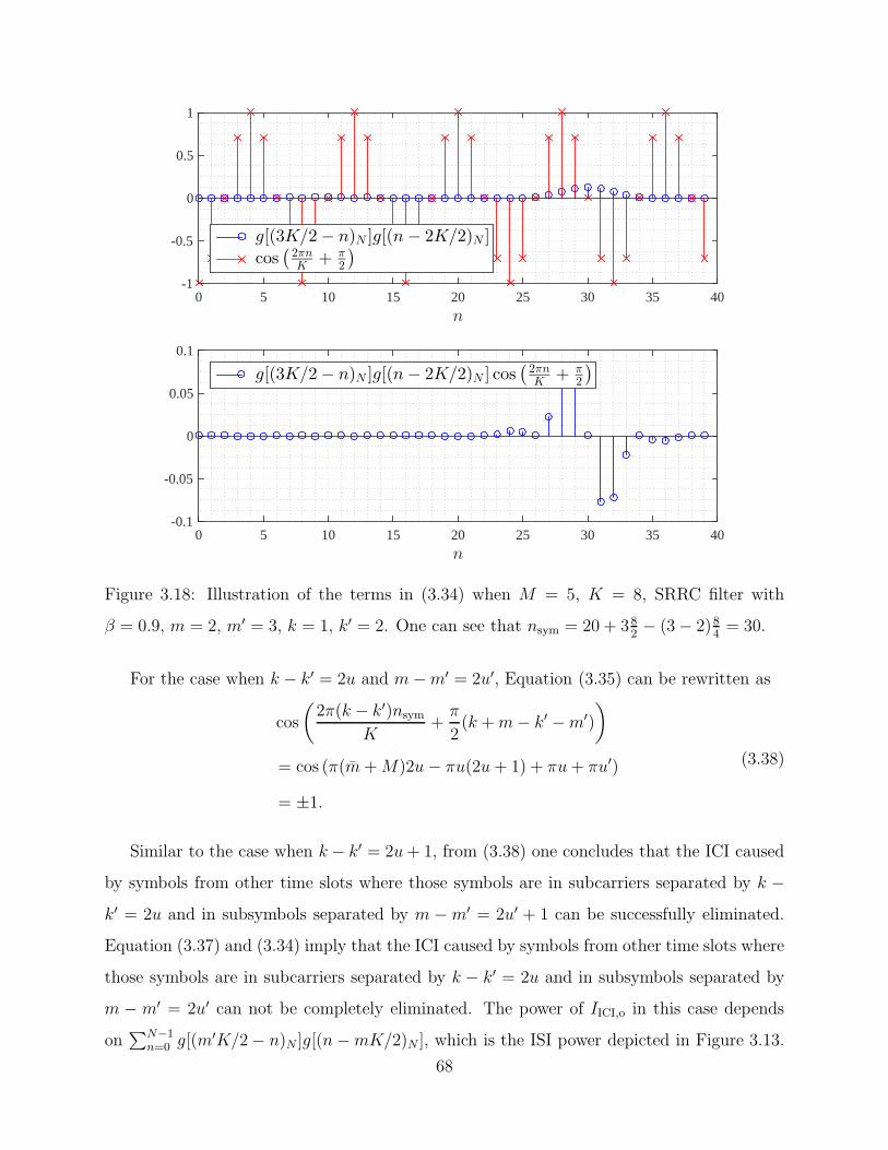
n0 5 10 15 20 25 30 35 40

-0.1

-0.05

0

0.05

0.1

g[(3K/2− n)N ]g[(n− 2K/2)N ] cos(

2πnK + π

2

)

n0 5 10 15 20 25 30 35 40

-1

-0.5

0

0.5

1

g[(3K/2− n)N ]g[(n− 2K/2)N ]

cos(

2πnK + π

2

)


β = 0.9, m = 2, m′ = 3, k = 1, k′ = 2. One can see that nsym = 20 + 382− (3− 2)8

4= 30.

For the case when k − k′ = 2u and m−m′ = 2u′, Equation (3.35) can be rewritten as

cos


K+

π

2(k +m− k′ −m′)

)

= cos (π(m+M)2u− πu(2u+ 1) + πu+ πu′)

= ±1.

(3.38)

Similar to the case when k − k′ = 2u+ 1, from (3.38) one concludes that the ICI caused

by symbols from other time slots where those symbols are in subcarriers separated by k −k′ = 2u and in subsymbols separated by m −m′ = 2u′ + 1 can be successfully eliminated.

Equation (3.37) and (3.34) imply that the ICI caused by symbols from other time slots where

those symbols are in subcarriers separated by k − k′ = 2u and in subsymbols separated by

m − m′ = 2u′ can not be completely eliminated. The power of IICI,o in this case depends

on∑N−1

n=0 g[(m′K/2− n)N ]g[(n−mK/2)N ], which is the ISI power depicted in Figure 3.13.

68

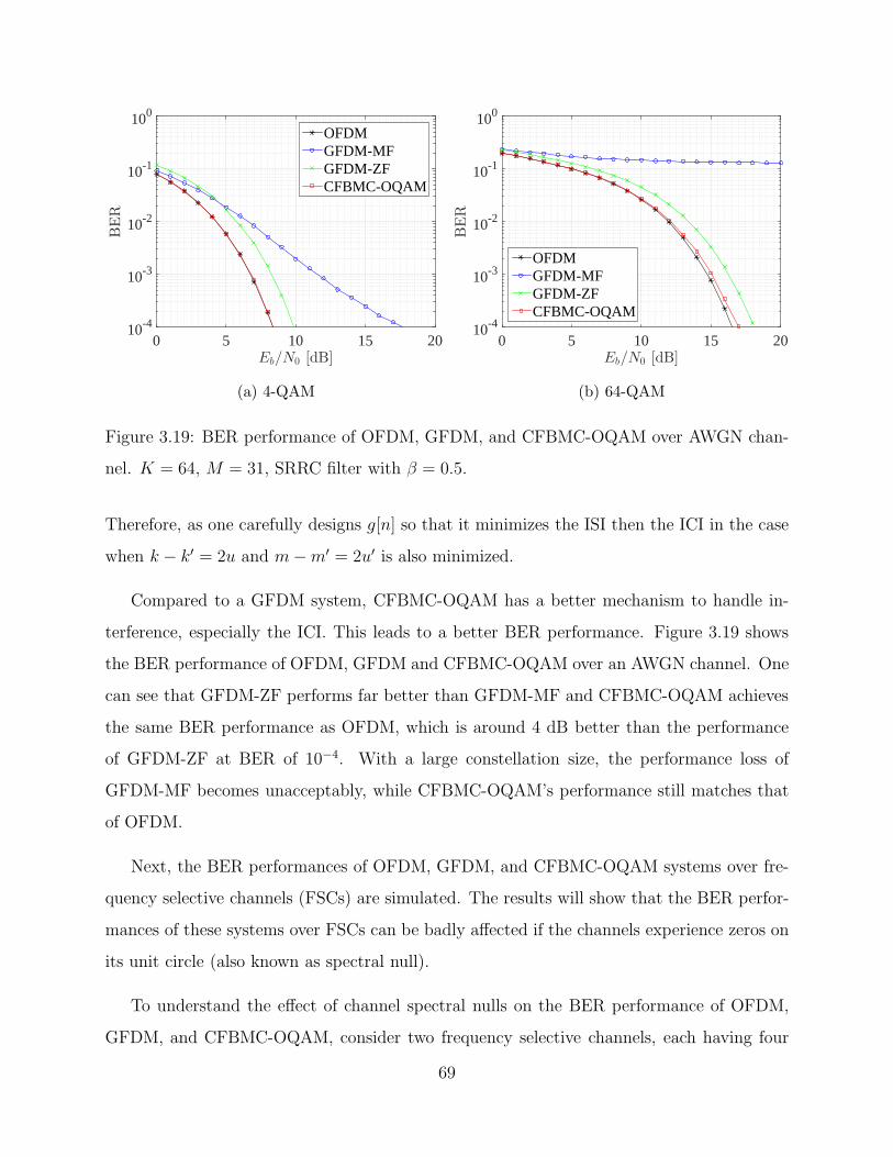
Eb/N0 [dB]0 5 10 15 20

BER

10-4

10-3

10-2

10-1

100

OFDMGFDM-MFGFDM-ZFCFBMC-OQAM

(a) 4-QAM

Eb/N0 [dB]0 5 10 15 20

BER

10-4

10-3

10-2

10-1

100

OFDMGFDM-MFGFDM-ZFCFBMC-OQAM

(b) 64-QAM

Figure 3.19: BER performance of OFDM, GFDM, and CFBMC-OQAM over AWGN chan-

nel. K = 64, M = 31, SRRC filter with β = 0.5.

Therefore, as one carefully designs g[n] so that it minimizes the ISI then the ICI in the case

when k − k′ = 2u and m−m′ = 2u′ is also minimized.

Compared to a GFDM system, CFBMC-OQAM has a better mechanism to handle in-

terference, especially the ICI. This leads to a better BER performance. Figure 3.19 shows

the BER performance of OFDM, GFDM and CFBMC-OQAM over an AWGN channel. One

can see that GFDM-ZF performs far better than GFDM-MF and CFBMC-OQAM achieves

the same BER performance as OFDM, which is around 4 dB better than the performance

of GFDM-ZF at BER of 10−4. With a large constellation size, the performance loss of

GFDM-MF becomes unacceptably, while CFBMC-OQAM’s performance still matches that

of OFDM.

Next, the BER performances of OFDM, GFDM, and CFBMC-OQAM systems over fre-

quency selective channels (FSCs) are simulated. The results will show that the BER perfor-

mances of these systems over FSCs can be badly affected if the channels experience zeros on

its unit circle (also known as spectral null).

To understand the effect of channel spectral nulls on the BER performance of OFDM,

GFDM, and CFBMC-OQAM, consider two frequency selective channels, each having four

69

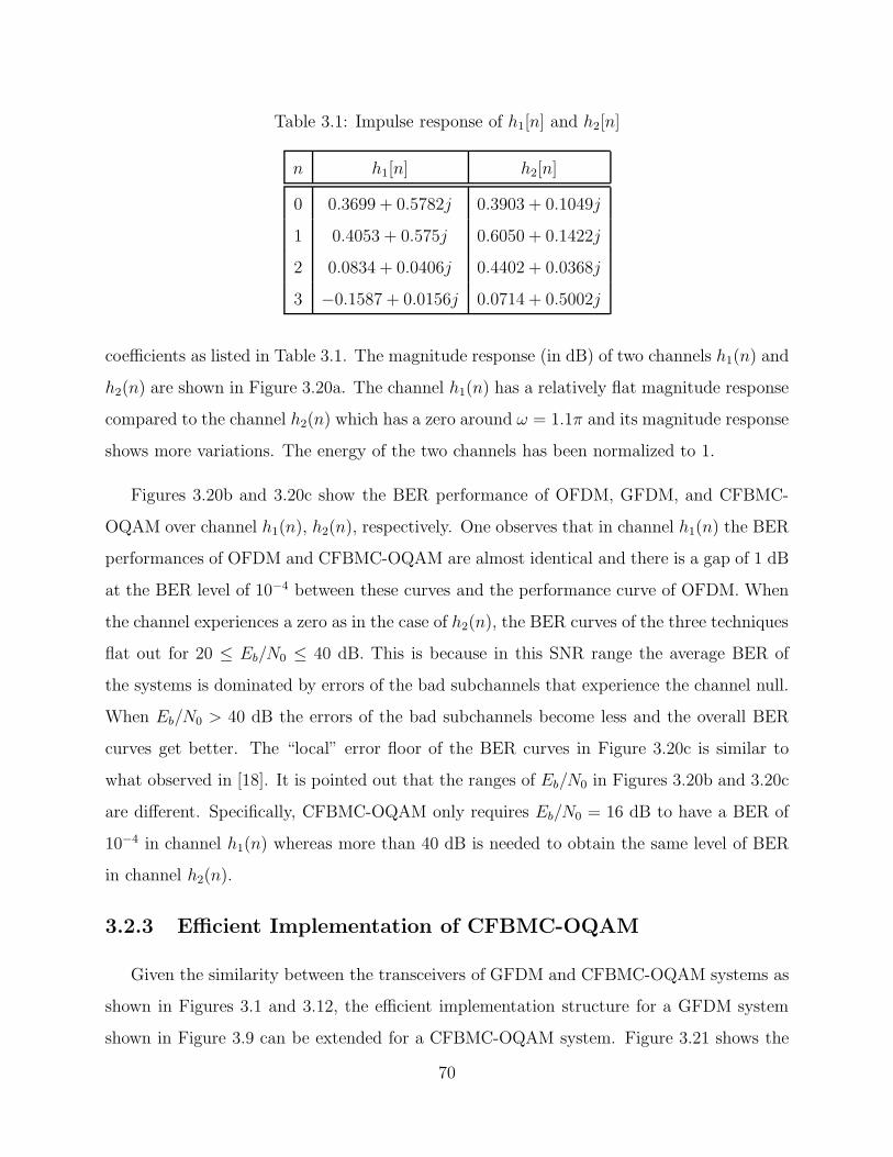
Table 3.1: Impulse response of h1[n] and h2[n]

n h1[n] h2[n]

0 0.3699 + 0.5782j 0.3903 + 0.1049j

1 0.4053 + 0.575j 0.6050 + 0.1422j

2 0.0834 + 0.0406j 0.4402 + 0.0368j

3 −0.1587 + 0.0156j 0.0714 + 0.5002j

coefficients as listed in Table 3.1. The magnitude response (in dB) of two channels h1(n) and

h2(n) are shown in Figure 3.20a. The channel h1(n) has a relatively flat magnitude response

compared to the channel h2(n) which has a zero around ω = 1.1π and its magnitude response

shows more variations. The energy of the two channels has been normalized to 1.

Figures 3.20b and 3.20c show the BER performance of OFDM, GFDM, and CFBMC-

OQAM over channel h1(n), h2(n), respectively. One observes that in channel h1(n) the BER

performances of OFDM and CFBMC-OQAM are almost identical and there is a gap of 1 dB

at the BER level of 10−4 between these curves and the performance curve of OFDM. When

the channel experiences a zero as in the case of h2(n), the BER curves of the three techniques

flat out for 20 ≤ Eb/N0 ≤ 40 dB. This is because in this SNR range the average BER of

the systems is dominated by errors of the bad subchannels that experience the channel null.

When Eb/N0 > 40 dB the errors of the bad subchannels become less and the overall BER

curves get better. The “local” error floor of the BER curves in Figure 3.20c is similar to

what observed in [18]. It is pointed out that the ranges of Eb/N0 in Figures 3.20b and 3.20c

are different. Specifically, CFBMC-OQAM only requires Eb/N0 = 16 dB to have a BER of

10−4 in channel h1(n) whereas more than 40 dB is needed to obtain the same level of BER

in channel h2(n).

3.2.3 Efficient Implementation of CFBMC-OQAM

Given the similarity between the transceivers of GFDM and CFBMC-OQAM systems as

shown in Figures 3.1 and 3.12, the efficient implementation structure for a GFDM system

shown in Figure 3.9 can be extended for a CFBMC-OQAM system. Figure 3.21 shows the

70

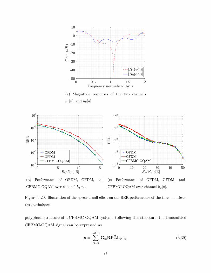
Frequency normalized by π0 0.5 1 1.5 2

Gain

(dB)

-50

-40

-30

-20

-10

0

10

|H1(ejω)|

|H2(ejω)|

(a) Magnitude responses of the two channels

h1[n], and h2[n]

Eb/N0 [dB]0 5 10 15

BER

10-4

10-3

10-2

10-1

100

OFDMGFDMCFBMC-OQAM

(b) Performance of OFDM, GFDM, and

CFBMC-OQAM over channel h1[n].

Eb/N0 [dB]0 10 20 30 40 50

BER

10-4

10-3

10-2

10-1

100

OFDMGFDMCFBMC-OQAM

(c) Performance of OFDM, GFDM, and

CFBMC-OQAM over channel h2[n].

Figure 3.20: Illustration of the spectral null effect on the BER performance of the three multicar-

riers techniques.

polyphase structure of a CFBMC-OQAM system. Following this structure, the transmitted

CFBMC-OQAM signal can be expressed as

x =

2M−1∑

m=0

GmRFHKJmam, (3.39)

71

where am is the mth column of matrix A in (3.26), Jm = diag([jm, jm+1, . . . , jm+K−1]) is

a matrix that introduces phase offsets, FK is the K-point FFT matrix, R = [IK , . . . , IK ]⊤

is the repetition matrix, Gm = diag(Φmg) = diag([g0,m, g1,m, . . . , gKM−1,m]), and Φm is a

KM ×KM circulant matrix whose first column has only one non zero value, which is the

(mK/2)th element with value 1. In this structure, am is first transformed into the time

domain by multiplying it with an inverse FFT matrix, FHK . Upsampling is performed by

repeating the K×1 transformed vector M times with the KM ×K matrix R. The resulted

vector is pulse-shaped by point-wise multiplication with the circularly shifted version of the

prototype filter, which is Φmg. Then the transmitted signal is obtained by summing all

pulse-shaped subsymbol vectors.

At the receiver, first, an equalizer S is applied to the received signal y to remove the

effect of multipath interference. Then, the equalized vector is processed in dual to (4.9).

The equalized output that can be used to detect the data symbols for the mth time slot is

given by

am = ℜ{JHmFKR

⊤GmSy}. (3.40)

3.3 Summay

This chapter has introduced GFDM and CFBMC-OQAM system. The two systems share

the same filtering process where circular convolution is utilized instead of linear convolution.

Using circular convolution for filtering allows the two systems to use filters which have

better stop-band attenuation than the rectangular filter used for OFDM systems without

increasing the length of CP. In addition, efficient implementation structure developed for a

GFDM system can be adapted for a CFBMC-OQAM system. The chapter also exlained

how GFDM and CFBMC-OQAM deal with ISI and ICI. A GFDM system, when using

MF receiver, lacks a mechanism to handle ICI, especially the severe ICI caused by symbols

from the adjacent subcarriers. Whereas, a CFBMC-OQAM system, due to the use of offset

QAM, can completely remove ICI from adjacent subcarriers. The simulation results which

compare the BER performance of GFDM and CFBMC-OQAM systems over AWGN and

FSC channels are also provided. It was demonstrated that the CFBMC-OQAM system is

72

ma

mj

mb

H

K

M

m mc

ma

mj

mb

K ma

m Kj

K mb

mg

mc

mg

mc

KM mg

KM mc

M

m mc

K m

M

mc

mg

mg

KM mg

K

mj

mj

m Kj

ma

ma

K ma

Figure 3.21: Efficient implementation of a CFBMC-OQAM system.

superior than the GFDM system. However, without additional processing techniques, the

BER performance of CFBMC-OQAM in FSCs might be significantly degraded due to the

spectral nulls effect. And thus more robust transceiver designs are required.

73

4. Walsh-Hadamard(WH)-CFBMC-OQAM

In the previous chapter, the transceiver structures of GFDM and CFBMC-OQAM sys-

tem were introduced. The key differences between those techniques were highlighted. In

particular, the advantages of CFBMC-OQAM over GFDM were illustrated. In addition,

it was pointed out that without additional processing techniques the BER performance of

OFDM, GFDM, and CFBMC-OQAM in frequency selective channels (FSCs) can be badly

affected if the channels have spectral nulls.

To have transceivers whose performance is more robust to channel nulls, many techniques

have been developed in the literature [8]. For example, in OFDM system with K subcarriers,

instead of transmitting K symbols on K subcarriers within one OFDM block, one can

transmit only L < K symbols on L subcarriers, where the choice of L subcarriers is different

for different OFDM blocks. This technique can achieve frequency diversity gain of K by

coding across the subcarriers within one OFDM block as well as across different blocks [7].

Another well known method to prevent the BER performance being dominated by the bad

subchannels is using a precoder, or using bit allocation techniques [33].

The focus of this chapter is on precoding schemes. There is a number of precoding

techniques that have been proposed for multicarreir systems. Those precoded schemes are

different in how they are designed and in their objectives. For example, the conventional CP-

OFDM system experiences high peak to average power ratio PAPR. Then one can consider

to use DFT precoder which is demontrated in [19] to produce very low PAPR. In fact, the

precoded scheme in [19] leads to the well-known single carrier system with cyclic prefix (SC-

CP) where the receiver performs both Discrete Fourier Transform (DFT) and Inverse DFT

(IDFT) operations. Another example is [16], which proposed precoded and vector OFDM to

74

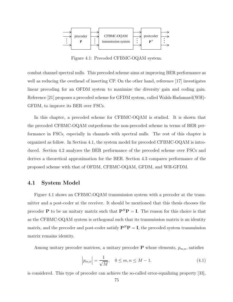
H

Figure 4.1: Precoded CFBMC-OQAM system.

combat channel spectral nulls. This precoded scheme aims at improving BER performance as

well as reducing the overhead of inserting CP. On the other hand, reference [17] investigates

linear precoding for an OFDM system to maximize the diversity gain and coding gain.

Reference [21] proposes a precoded scheme for GFDM system, called Walsh-Hadamard(WH)-

GFDM, to improve its BER over FSCs.

In this chapter, a precoded scheme for CFBMC-OQAM is studied. It is shown that

the precoded CFBMC-OQAM outperforms the non-precoded scheme in terms of BER per-

formance in FSCs, especially in channels with spectral nulls. The rest of this chapter is

organized as follow. In Section 4.1, the system model for precoded CFBMC-OQAM is intro-

duced. Section 4.2 analyzes the BER performance of the precoded scheme over FSCs and

derives a theoretical approximation for the BER. Section 4.3 compares performance of the

proposed scheme with that of OFDM, CFBMC-OQAM, GFDM, and WH-GFDM.

4.1 System Model

Figure 4.1 shows an CFBMC-OQAM transmission system with a precoder at the trans-

mitter and a post-coder at the receiver. It should be mentioned that this thesis chooses the

precoder P to be an unitary matrix such that PHP = I. The reason for this choice is that

as the CFBMC-OQAM system is orthogonal such that its transmission matrix is an identity

matrix, and the precoder and post-coder satisfy PHP = I, the precoded system transmission

matrix remains identity.

Among unitary precoder matrices, a unitary precoder P whose elements, pm,n, satisfies

∣∣∣pm,n

∣∣∣ =

1√M

, 0 ≤ m,n ≤ M − 1. (4.1)

is considered. This type of precoder can achieve the so-called error-equalizing property [33],

75

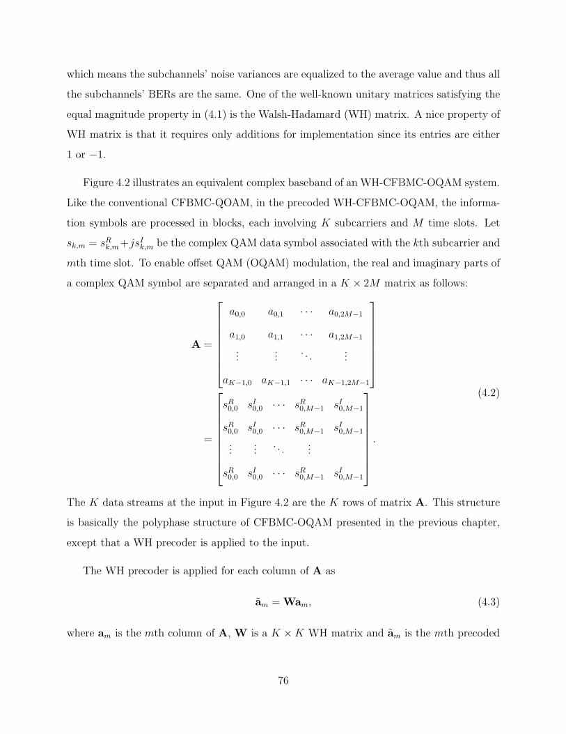
which means the subchannels’ noise variances are equalized to the average value and thus all

the subchannels’ BERs are the same. One of the well-known unitary matrices satisfying the

equal magnitude property in (4.1) is the Walsh-Hadamard (WH) matrix. A nice property of

WH matrix is that it requires only additions for implementation since its entries are either

1 or −1.

Figure 4.2 illustrates an equivalent complex baseband of an WH-CFBMC-OQAM system.

Like the conventional CFBMC-QOAM, in the precoded WH-CFBMC-OQAM, the informa-

tion symbols are processed in blocks, each involving K subcarriers and M time slots. Let

sk,m = sRk,m+jsIk,m be the complex QAM data symbol associated with the kth subcarrier and

mth time slot. To enable offset QAM (OQAM) modulation, the real and imaginary parts of

a complex QAM symbol are separated and arranged in a K × 2M matrix as follows:

A =

a0,0 a0,1 · · · a0,2M−1

a1,0 a1,1 · · · a1,2M−1

......

. . ....

aK−1,0 aK−1,1 · · · aK−1,2M−1

=

sR0,0 sI0,0 · · · sR0,M−1 sI0,M−1

sR0,0 sI0,0 · · · sR0,M−1 sI0,M−1

......

. . ....

sR0,0 sI0,0 · · · sR0,M−1 sI0,M−1

.

(4.2)

The K data streams at the input in Figure 4.2 are the K rows of matrix A. This structure

is basically the polyphase structure of CFBMC-OQAM presented in the previous chapter,

except that a WH precoder is applied to the input.

The WH precoder is applied for each column of A as

am = Wam, (4.3)

where am is the mth column of A, W is a K ×K WH matrix and am is the mth precoded

76

mama

mj

mb

K H

K

M

m mc

ma

mj

mb

K ma

m Kj

K mb

ma

K ma

mg

mc

mg

mc

KM mg

KM mc

M

m mc

K m

M

mc

mg

mg

KM mg

K

mj

mj

m Kj

K

ma

ma

K ma

Figure 4.2: Equivalent complex baseband WH-CFBMC-OQAM system.

column vector.

WK =1√K

WK/2 WK/2

WK/2 −WK/2

, W2 =1√2

1 1

1 −1

. (4.4)

Similar to the conventional CFBMC-OQAM, the phase offsets are introduced to the real

and imaginary components of QAM symbols on different subcarriers as follows:

bm = Jmam (4.5)

where Jm = diag([jm, jm+1, . . . , jm+K−1]). Then, the WH-CFBMC-OQAM transmitted sig-

nal is given as [34]

x[n] =

K−1∑

k=0

2M−1∑

m=0

jk+mak,mg[(n−mK/2)N ]ej2πkn/K , (4.6)

where n = 0, 1, . . . , N = KM −1, ak,m is the kth element of am, g[n] is the impulse response

of a prototype filter, which has KM coefficients, and g[(n− z)w] denotes cyclically shifting

g[n] by z positions with period w.

77

The polyphase structure [15] for the implementation of (4.6) as shown in Fig. 4.2 is the

most efficient method and can be described clearly in matrix form. Let

x = [x[0], x[1], . . . , x[KM − 1]]⊤, (4.7)

and g = [g[0], g[1], . . . , g[KM−1]]⊤ be the transmitted vector and vector of filter coefficients,

respectively. Then the matrix form representation of (4.6) is

x =

2M−1∑

m=0

GmRFHbm, (4.8)

where F is the K-point FFT matrix, R = [IK , . . . , IK]⊤, Gm = diag(Φmg) and Φm is a

KM ×KM circulant matrix whose first column has only one non zero value, which is the

(mK/2)th element with value 1. In this structure, bm is first transformed into the time

domain by multiplying it with an inverse FFT matrix, FH . Upsampling is performed by

repeating the K×1 transformed vector M times with the KM ×K matrix R. The resulted

vector is pulse-shaped by point-wise multiplication with the circularly shifted version of the

prototype filter, which is Φmg. Then the transmitted signal is obtained by summing all

pulse-shaped subsymbol vectors. Substituting (4.3) and (4.5) into (4.8), the transmitted

signal of WH-CFBMC-OQAM can be expressed as

x =

2M−1∑

m=0

GmRFHJmWam. (4.9)

In a frequency selective channel, WH-CFBMC-OQAM uses a cyclic prefix (CP) of length

L to achieve free inter-block interference (IBI). Let h = [h[0], h[1], · · · , h[V −1]]⊤ (V ≪ N =

MK − 1) be the vector of an V -taps channel impulse response. As long as V − 1 ≤ L, free

IBI is guaranteed at the receiver. In that case, the received signal after removing CP can be

written as

y = Hx+ n, (4.10)

where H is a KM × KM circulant matrix whose first column is h appended with N − V

zeros, and n is a vector of additive while Gaussian noise (AWGN) samples.

An approach to demodulate data is described in Fig. 4.2 [15]. First, an equalizer S is

applied to the received signal y to remove the effect of multipath interference. Then, the

78

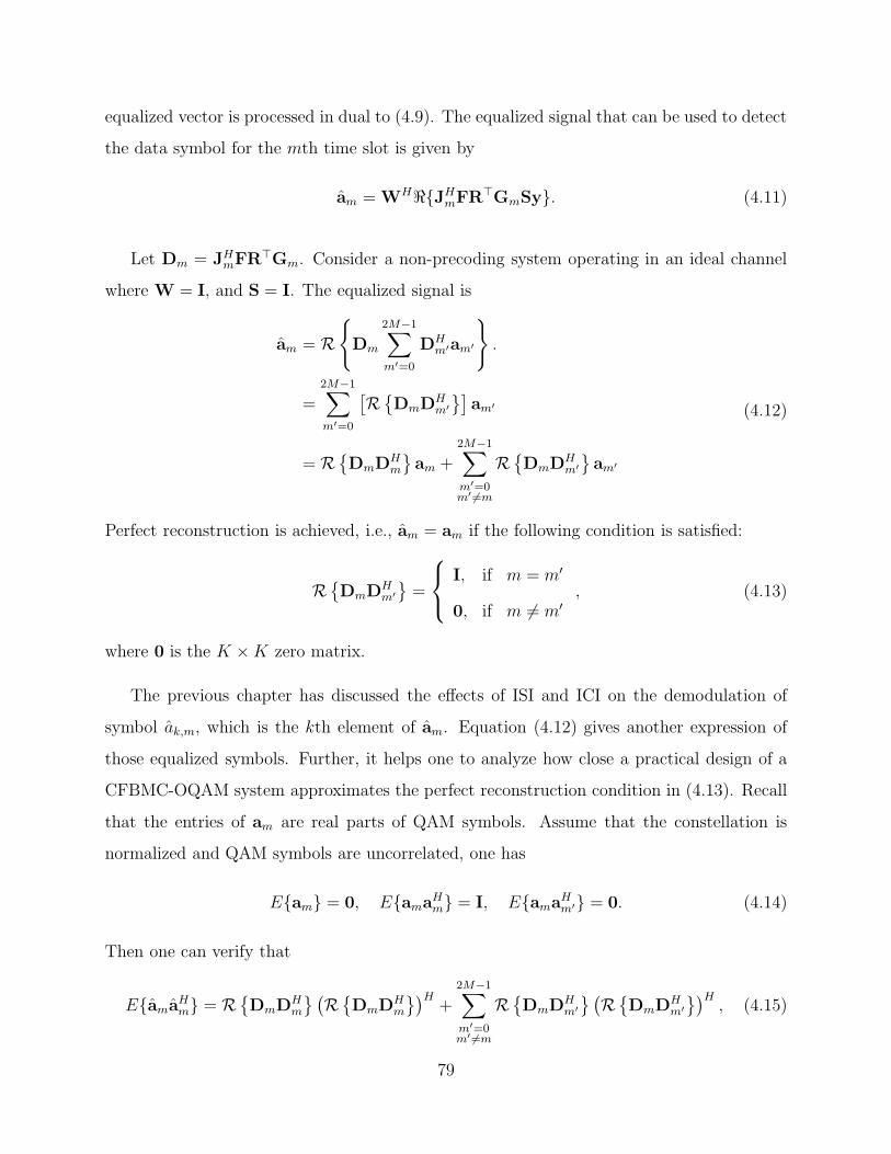
equalized vector is processed in dual to (4.9). The equalized signal that can be used to detect

the data symbol for the mth time slot is given by

am = WHℜ{JHmFR

⊤GmSy}. (4.11)

Let Dm = JHmFR

⊤Gm. Consider a non-precoding system operating in an ideal channel

where W = I, and S = I. The equalized signal is

am = R{

Dm

2M−1∑

m′=0

DHm′am′

}

.

=2M−1∑

m′=0

[R{DmD

Hm′

}]am′

= R{DmD

Hm

}am +

2M−1∑

m′=0m′ 6=m

R{DmD

Hm′

}am′

(4.12)

Perfect reconstruction is achieved, i.e., am = am if the following condition is satisfied:

R{DmD

Hm′

}=

I, if m = m′

0, if m 6= m′, (4.13)

where 0 is the K ×K zero matrix.

The previous chapter has discussed the effects of ISI and ICI on the demodulation of

symbol ak,m, which is the kth element of am. Equation (4.12) gives another expression of

those equalized symbols. Further, it helps one to analyze how close a practical design of a

CFBMC-OQAM system approximates the perfect reconstruction condition in (4.13). Recall

that the entries of am are real parts of QAM symbols. Assume that the constellation is

normalized and QAM symbols are uncorrelated, one has

E{am} = 0, E{amaHm} = I, E{ama

Hm′} = 0. (4.14)

Then one can verify that

E{amaHm} = R

{DmD

Hm

} (R{DmD

Hm

})H+

2M−1∑

m′=0m′ 6=m

R{DmD

Hm′

} (R{DmD

Hm′

})H, (4.15)

79

10 20 30 40 50 60

10

20

30

40

50

60-200

-150

-100

-50

0

(a) R{DmD

Hm

} (R{DmD

Hm

})H

10 20 30 40 50 60

10

20

30

40

50

60

-200

-150

-100

(b)∑2M−1

m′=0m′ 6=m

R{DmD

Hm′

} (R{DmD

Hm′

})H

10 20 30 40 50 60

10

20

30

40

50

60-200

-150

-100

-50

0

(c) E{amaHm}

Figure 4.3: Visualization of the terms in Equation (4.15).

where E{amaHm} is a covariance matrix that characterizes the correlation between entries of

am. Entry [E{amaHm}]k,k′ is the interference power caused by ak′,m when one demodulates

ak,m. The first term on the right hand side of (4.15) represents the ICI caused by symbols

from the same time slots, and the second term represents the ICI caused by symbols from

all other time slots. Figure 4.3 illustrates these terms for a CFBMC-OQAM system with

K = 64, M = 15, and an SRRC filter (β = 0.9). The ICI power in this example is

summarized in Table 4.1. Notice that the ISI power when m 6= m′ is significantly lower

than that when m = m′. Overall, E{amaHm} has a diagonal structure as illustrated in Figure

4.3c. This particular example shows that a design of CFBMC-OQAM where a SRRC filter

80

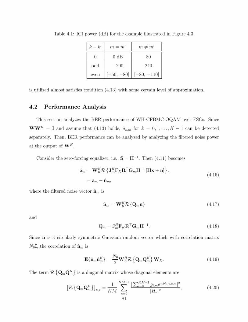
Table 4.1: ICI power (dB) for the example illustrated in Figure 4.3.

k − k′ m = m′ m 6= m′

0 0 dB −80

odd −200 −240

even [−50, −80] [−80, −110]

is utilized almost satisfies condition (4.13) with some certain level of approximation.

4.2 Performance Analysis

This section analyzes the BER performance of WH-CFBMC-OQAM over FSCs. Since

WWH = I and assume that (4.13) holds, ak,m for k = 0, 1, . . . , K − 1 can be detected

separately. Then, BER performance can be analyzed by analyzing the filtered noise power

at the output of WH .

Consider the zero-forcing equalizer, i.e., S = H−1. Then (4.11) becomes

am = WHKR

{JHmFKR

⊤GmH−1 [Hx+ n]

}.

= am + nm,(4.16)

where the filtered noise vector nm is

nm = WHKR{Qmn} (4.17)

and

Qm = JHmFKR

⊤GmH−1. (4.18)

Since n is a circularly symmetric Gaussian random vector which with correlation matrix

N0I, the correlation of nm is

E{nmnHm} =

N0

2WH

KR{QmQ

Hm

}WK . (4.19)

The term R{QmQ

Hm

}is a diagonal matrix whose diagonal elements are

[R{QmQ

Hm

}]

k,k=

1

KM

KM−1∑

n=0

|∑KM−1i=0 gi,me

−jφi,n,k,m|2|Hn|2

, (4.20)

81

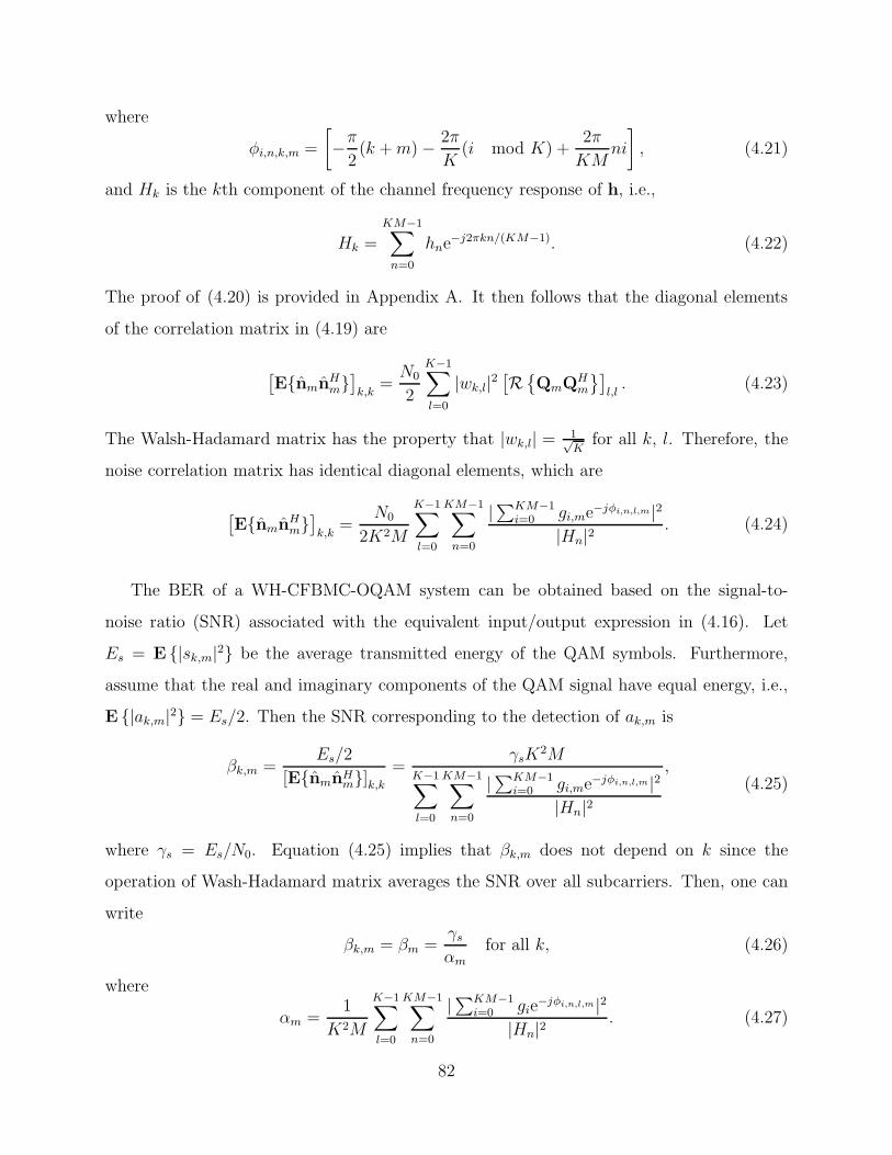
where

φi,n,k,m =

[

−π

2(k +m)− 2π

K(i mod K) +

2π

KMni

]

, (4.21)

and Hk is the kth component of the channel frequency response of h, i.e.,

Hk =

KM−1∑

n=0

hne−j2πkn/(KM−1). (4.22)

The proof of (4.20) is provided in Appendix A. It then follows that the diagonal elements

of the correlation matrix in (4.19) are

[E{nmn

Hm}]

k,k=

N0

2

K−1∑

l=0

|wk,l|2[R{QmQ

Hm

}]

l,l. (4.23)

The Walsh-Hadamard matrix has the property that |wk,l| = 1√K

for all k, l. Therefore, the

noise correlation matrix has identical diagonal elements, which are

[E{nmn

Hm}]

k,k=

N0

2K2M

K−1∑

l=0

KM−1∑

n=0

|∑KM−1i=0 gi,me

−jφi,n,l,m|2|Hn|2

. (4.24)

The BER of a WH-CFBMC-OQAM system can be obtained based on the signal-to-

noise ratio (SNR) associated with the equivalent input/output expression in (4.16). Let

Es = E {|sk,m|2} be the average transmitted energy of the QAM symbols. Furthermore,

assume that the real and imaginary components of the QAM signal have equal energy, i.e.,

E {|ak,m|2} = Es/2. Then the SNR corresponding to the detection of ak,m is

βk,m =Es/2

[E{nmnHm}]k,k

=γsK

2MK−1∑

l=0

KM−1∑

n=0

|∑KM−1i=0 gi,me


,(4.25)

where γs = Es/N0. Equation (4.25) implies that βk,m does not depend on k since the

operation of Wash-Hadamard matrix averages the SNR over all subcarriers. Then, one can

write

βk,m = βm =γsαm

for all k, (4.26)

where

αm =1

K2M

K−1∑

l=0

KM−1∑

n=0

|∑KM−1i=0 gie


. (4.27)

82

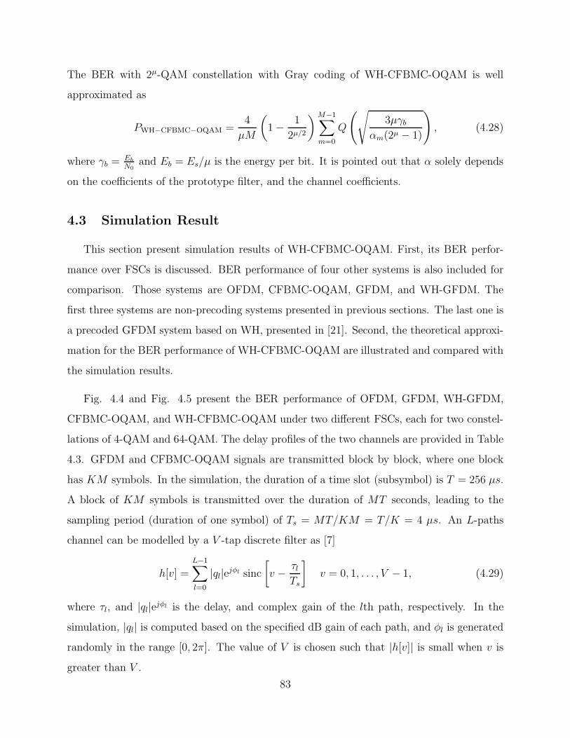
The BER with 2µ-QAM constellation with Gray coding of WH-CFBMC-OQAM is well

approximated as

PWH−CFBMC−OQAM =4

µM

(

1− 1

2µ/2

)M−1∑

m=0

Q

(√

3µγbαm(2µ − 1)

)

, (4.28)

where γb =Eb

N0and Eb = Es/µ is the energy per bit. It is pointed out that α solely depends

on the coefficients of the prototype filter, and the channel coefficients.

4.3 Simulation Result

This section present simulation results of WH-CFBMC-OQAM. First, its BER perfor-

mance over FSCs is discussed. BER performance of four other systems is also included for

comparison. Those systems are OFDM, CFBMC-OQAM, GFDM, and WH-GFDM. The

first three systems are non-precoding systems presented in previous sections. The last one is

a precoded GFDM system based on WH, presented in [21]. Second, the theoretical approxi-

mation for the BER performance of WH-CFBMC-OQAM are illustrated and compared with

the simulation results.

Fig. 4.4 and Fig. 4.5 present the BER performance of OFDM, GFDM, WH-GFDM,

CFBMC-OQAM, and WH-CFBMC-OQAM under two different FSCs, each for two constel-

lations of 4-QAM and 64-QAM. The delay profiles of the two channels are provided in Table

4.3. GFDM and CFBMC-OQAM signals are transmitted block by block, where one block

has KM symbols. In the simulation, the duration of a time slot (subsymbol) is T = 256 µs.

A block of KM symbols is transmitted over the duration of MT seconds, leading to the

sampling period (duration of one symbol) of Ts = MT/KM = T/K = 4 µs. An L-paths

channel can be modelled by a V -tap discrete filter as [7]

h[v] =

L−1∑

l=0

|ql|ejφl sinc

[

v − τlTs

]

v = 0, 1, . . . , V − 1, (4.29)

where τl, and |ql|ejφl is the delay, and complex gain of the lth path, respectively. In the

simulation, |ql| is computed based on the specified dB gain of each path, and φl is generated

randomly in the range [0, 2π]. The value of V is chosen such that |h[v]| is small when v is

greater than V .

83

Table 4.2: Simulation parameters.

Parameters Value

Number of subcarriers (K) 64

Number of subsymbols (M) 31

Prototype filter SRRC

Roll-off 0.9

Modulation 4-QAM, 64-QAM

Table 4.3: Delay profile used in simulation.

Channel A Gain (dB) 0 −8 −14 - - - -

Delay (µs) 0 4.57 9.14 - - - -

Channel B Gain (dB) 0 −10 −12 −13 −16 −20 −22

Delay (µs) 0 2.85 4.57 6.28 9.71 15.43 20

Fig. 4.4 shows that WH-CFBMC-OQAM performs 2.5 dB better than WH-GFDM at

the BER level of 10−4 even with a large constellation such as 64-QAM. Since WH-GFDM

is based on GFDM, which is a non-orthogonal system, the interference between subsymbols

and subcarriers is intensified in a FSC. That makes the BER performances of WH-GFDM

worse than that of WH-CFBMC-OQAM. WH-GFDM and WHT-CFBMC-OQAM offer even

a larger performance gain under Channel B. Specifically, WH-GFDM is 5 dB better than

the non-precoding scheme, while WH-CFBMC-OQAM achieves 7.5 dB SNR gain at BER

= 10−4.

Fig. 4.6 shows that (4.28) can be used to accurately estimate the BER of WHT-C-

FBMC over a FSC. In both channels, with 4-QAMmodulation, the theoretical result matches

perfectly with that of the simulation result for any SNR value. With 64-QAM modulation,

the theoretical approximation is very accurate at SNR larger than 7.5 dB.

84

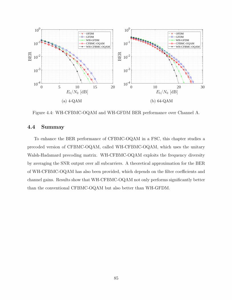
0 5 10 15 2010-4

10-3

10-2

10-1

100

OFDMGFDMWH-GFDMCFBMC-OQAMWH-CFBMC-OQAM

(a) 4-QAM

0 10 20 3010-4

10-3

10-2

10-1

100


(b) 64-QAM

Figure 4.4: WH-CFBMC-OQAM and WH-GFDM BER performance over Channel A.

4.4 Summay

To enhance the BER performance of CFBMC-OQAM in a FSC, this chapter studies a

precoded version of CFBMC-OQAM, called WH-CFBMC-OQAM, which uses the unitary

Walsh-Hadamard precoding matrix. WH-CFBMC-OQAM exploits the frequency diversity

by averaging the SNR output over all subcarriers. A theoretical approximation for the BER

of WH-CFBMC-OQAM has also been provided, which depends on the filter coefficients and

channel gains. Results show that WH-CFBMC-OQAM not only performs significantly better

than the conventional CFBMC-OQAM but also better than WH-GFDM.

85

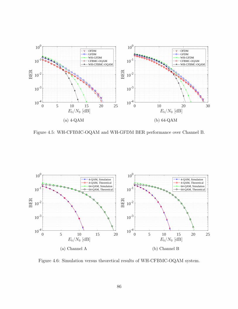
0 5 10 15 20 2510-4

10-3

10-2

10-1

100


(a) 4-QAM

0 10 20 3010-4

10-3

10-2

10-1

100


(b) 64-QAM

Figure 4.5: WH-CFBMC-OQAM and WH-GFDM BER performance over Channel B.

0 5 10 15 2010-4

10-3

10-2

10-1

100

4-QAM, Simulation4-QAM, Theoretical64-QAM, Simulation64-QAM, Theoretical

(a) Channel A

0 5 10 15 20 2510-4

10-3

10-2

10-1

100

4-QAM, Simulation4-QAM, Theoretical64-QAM, Simulation64-QAM, Theoretical

(b) Channel B

Figure 4.6: Simulation versus theoretical results of WH-CFBMC-OQAM system.

86

5. Conclusion and Suggestion for Further

Research

5.1 Conclusion

This thesis studies candidate multicarrier transmission techniques for 5G systems. First,

a classic cyclic prefix OFDM system is presented. Due to its efficient implementation via

FFT/IFFT blocks and simple frequency domain equalizer, OFDM is still a candidate for

5G. However, its main weaknesses, high side lobes and low spectral efficiency, motivate

researchers to find potential alternatives.

Filter bank multicarrier offset QAM (FBMC-OQAM) and generalized frequency divi-

sion multiplexing (GFDM) are two multicarrier techniques which are actively investigated.

FBMC-OQAM addresses the drawback of rectangular time windowing in OFDM by using a

prototype filter that satisfies the Nyquist condition. The orthogonality between subcarriers

in FBMC-OQAM is achieved by using offset QAM. However, unlike OFDM, FBMC-OQAM

does not have a block-based structure to facilitate an efficient implementation as well as

a simple equalization. In constrast, GFDM has a block-based structure. It exploits that

structure to replace the linear convolution in filtering with circular convolution. By doing

so, the length of the cyclic prefix (CP) does not need to take into account the length of the

filter and thus the overhead due to the use of the CP can be reduced. Unfortunately, GFDM

is not an orthogonal system. The non-orthogonality between subcarriers requires a complex

receiver to cancel intercarrier interference.

Recently, circular filter bank multicarrier offset QAM (CFBMC-OQAM) is proposed,

which combines two key features, the offset QAM of the conventional FBMC-OQAM and the

87

block-based structure and circular convolution of GFDM in one system. The combination

makes CFBMC-OQAM not only being an orthogonal system as FBMC-OQAM but also

having an efficient implementation structure and simple equalization as GFDM.

The main contribution of this thesis is developing and analyzing a precoded scheme for

CFBMC-OQAM is studied. In particular, WH-CFBMC-OQAM, which applies the Walsh-

Hadamard transform to the CFBMC-OQAM system, has been developed. The objective

of the precoded scheme is to make WH-CFBMC-OQAM more robust in frequency selec-

tive channels than FBMC-OQAM, GFDM, and CFBMC-OQAM. To estimate the BER

performance of WH-CFBMC-OQAM over FSCs a theoretical approximation is derived. Un-

der FSCs, simulation results show a significant performance improvement of WH-CFBMC-

OQAM. Under the same system parameters setup, WH-CFBMC-OQAM is shown to out-

perform the non-precoded system, OFDM, FBMC-OQAM, CFBMC-OQAM, GFDM, and

also the precoded system, WH-GFDM.

While the Walsh-Hadamard (WH) transform is proposed for precoding in this thesis, the

framework and the performance analysis can be carried out for other unitary matrix trans-

forms. For a simple implementation, WH is chosen since its entries are just real numbers.

One may use other transforms to meet different objectives. For example, a CAZAC uni-

tary transform [35] can be considered for further reducing the peak-to-average power ratio

(PAPR) as suggested in [36].

The theoretical approximation of the BER performance of WH-CFBMC-OQAM under

FSCs derived in this thesis could potentially be helpful in the designing of a prototype

filter for an WH-CFBMC-OQAM system. Specifically, since the theoretical approximation

depends on the coefficients of the prototype filter, one can use it to design an optimal filter

for WH-CFBMC-OQAM that minimizes the BER.

5.2 Suggestion for Further Research

To meet the challenging objectives of 5G networks, researchers have studied new and

more effective PHY techniques. There has been a growing interest on index modulation

88

(IM) over the past few years. IM is a new digital modulation scheme with high spectral and

energy efficiency, in which the indices of the building blocks of the considered communica-

tions system are utilized to transmit additional information bits [37]. Reference [38] perhaps

is the first to propose a technique called spatial modulation (SM), which is IM in the spatial

domain. In this technique the indices of antennas are utilized to convey additional infor-

mation bits. This technique has an advantage that only one antenna at the transmitter is

active. The receiver’s complexity of SM is reduced significantly compared to its competitors

such as vertical Bell Labs layered space-time (V-BLAST) and space-time coding (STC) sys-

tems. Inspired by index modulation in the spatial domain, researchers have explored index

modulation in the frequency domain as well. In particular, reference [39] proposed OFDM-

IM where an incoming bit stream is split into index selection bits and M-ary constellation

bits. The index selection bits determine a subset of subcarriers and those subcarriers are set

to active while other subcarriers are off. CFBMC-OQAM and WH-CFBMC-OQAM have

a block based structure like OFDM and thus the IM concept can be applied to these two

schemes. In addition, the separation between real and imaginary parts of complex symbols

in CFBMC-OQAM might result in a different way to manipulate indicies of subcarriers.

Applying IM in CFBMC-OQAM systems is a promising research topic.

89

Appendix

From (4.18), R{QmQ

Hm

}is given as

R{QmQ

Hm

}= R

{JHmFKR

⊤GmH−1(H−1)HGmRFH

KJm

}(A.1)

Recall thatH is aKM×KM circulant matrix. Thus, one hasH−1(H−1)H = 1KM

FHKMΛFKM ,

where Λ = diag(|H0|−2, |H1|−2, . . . , |HKM−1|−2). Rewrite (A.1) as

R{QmQ

Hm

}=

1

KMR{TmΛTH

m

}(A.2)

where

Tm = YmFHKM , Ym = JH

mFKR⊤Gm. (A.3)

The (k, n) elements of Tm are

tk,n =

KM−1∑

i=0

yk,iej 2πKM

ni, (A.4)

where

yk,i = (−j)k+mgi,me−j 2π

Kk(i mod K). (A.5)

Thus, the elements of R{QmQ

Hm

}are

[R{QmQ

Hm

}]k,k′ =

1

KM

∑KM−1n=0 R{tk,n(tk′,n)∗}

|Hn|2(A.6)

For k = k′, it is easy to see that using (A.4) and (A.5) leads to the expression of[R{QmQ

Hm

}]

k,kin (4.20).

90

For k 6= k′, one has

R{tk,n(tk′,n)∗} = R{

KM−1∑

i=0

yk,iej 2πKM

ni

KM−1∑

i′=0

(yk′,i′)∗e−j 2π

KMni′

}

= R{

KM−1∑

i=0

yk,i(yk′,i)∗

}

+R

KM−1∑

i=0

yk,iej 2πKM

ni

KM−1∑

i′=0i′ 6=i

yk′,i′e−j 2π

KMni′

(A.7)

From (4.13), and (A.5) it can be verified that R{∑KM−1

i=0 yk,i(yk′,i)∗}

= 0. In addition,

from (A.5) and the fact that gKM−i,m = gi,m for i < KM2, one has

yk,KM−i = (−j)k+mgKM−i,me−j 2π

Kk(KM−i mod K)

= (−j)k+mgi,mej 2π

Kk(i mod K).

(A.8)

Using (A.5), and (A.8), one can verify that

R{yk,i(yk′,i′)∗} = −R{yk,KM−i(y

mk′,KM−i′)

∗}

I {yk,i(yk′,i′)∗} = I{yk,KM−i(y

mk′,KM−i′)

∗} .(A.9)

Thus, (A.7) can be rewritten as

R{tk,n(tk′,n)∗}

=

KM/2−1∑

i=0

R{[

yk,i(yk′,i′)∗ej

2πKM

n(i−i′) + yk,KM−i(ymk′,KM−i′)

∗e−j 2πKM

n(i−i′)]}

=

KM/2−1∑

i=0

[

R{yk,i(yk′,i′)∗} cos2π

KMn(i− i′)− I {yk,i(yk′,i′)∗} sin

2π

KMn(i− i′)

+R{yk,KM−i(yk′,KM−i′)∗} cos 2π

KMn(i− i′) + I {yk,KM−i(yk′,KM−i′)

∗} sin 2π

KMn(i− i′)

]

= 0.

(A.10)

91

References

[1] F. Boccardi, R. W. Heath, A. Lozano, T. L. Marzetta, and P. Popovski, “Five disruptive

technology directions for 5G,” IEEE Communications Magazine, vol. 52, pp. 74–80,

February 2014.

[2] J. G. Andrews, S. Buzzi, W. Choi, S. V. Hanly, A. Lozano, A. C. K. Soong, and

J. C. Zhang, “What will 5G be?,” IEEE Journal on Selected Areas in Communications,

vol. 32, pp. 1065–1082, June 2014.

[3] C. X. Wang, F. Haider, X. Gao, X. H. You, Y. Yang, D. Yuan, H. M. Aggoune, H. Haas,

S. Fletcher, and E. Hepsaydir, “Cellular architecture and key technologies for 5G wire-

less communication networks,” IEEE Communications Magazine, vol. 52, pp. 122–130,

February 2014.

[4] T. S. Rappaport, S. Sun, R. Mayzus, H. Zhao, Y. Azar, K. Wang, G. N. Wong, J. K.

Schulz, M. Samimi, and F. Gutierrez, “Millimeter wave mobile communications for 5G

cellular: It will work!,” IEEE Access, vol. 1, pp. 335–349, 2013.

[5] C. Han, T. Harrold, S. Armour, I. Krikidis, S. Videv, P. M. Grant, H. Haas, J. S. Thomp-

son, I. Ku, C. X. Wang, T. A. Le, M. R. Nakhai, J. Zhang, and L. Hanzo, “Green radio:

radio techniques to enable energy-efficient wireless networks,” IEEE Communications

Magazine, vol. 49, pp. 46–54, June 2011.

[6] A. Osseiran, F. Boccardi, V. Braun, K. Kusume, P. Marsch, M. Maternia, O. Queseth,

M. Schellmann, H. Schotten, H. Taoka, H. Tullberg, M. A. Uusitalo, B. Timus, and

M. Fallgren, “Scenarios for 5G mobile and wireless communications: the vision of the

METIS project,” IEEE Communications Magazine, vol. 52, pp. 26–35, May 2014.

[7] D. Tse and P. Viswanath, Fundamentals of wireless communication. New York, NY,

USA: Cambridge University Press, 2005.

92

[8] A. Goldsmith, Wireless communications. New York, NY, USA: Cambridge University

Press, 2005.

[9] Proakis, Digital communications 5th edition. McGraw Hill, 2007.

[10] A. Sahin, I. Guvenc, and H. Arslan, “A survey on multicarrier communications: Pro-

totype filters, lattice structures, and implementation aspects,” IEEE Communications

Surveys Tutorials, vol. 16, pp. 1312–1338, Third Quarter 2014.

[11] T. Hwang, C. Yang, G. Wu, S. Li, and G. Y. Li, “OFDM and its wireless applications:

A survey,” IEEE Transactions on Vehicular Technology, vol. 58, pp. 1673–1694, May

2009.

[12] B. Farhang-Boroujeny, “OFDM versus filter bank multicarrier,” IEEE Signal Processing

Magazine, vol. 28, pp. 92–112, May 2011.

[13] G. Fettweis, M. Krondorf, and S. Bittner, “GFDM-generalized frequency division mul-

tiplexing,” in Proceedings IEEE Vehicular Technology Conference, pp. 1–4, April 2009.

[14] R. Datta, N. Michailow, M. Lentmaier, and G. Fettweis, “GFDM interference cancella-

tion for flexible cognitive radio PHY design,” in Proceedings IEEE Vehicular Technology

Conference, September 2012.

[15] H. Lin and P. Siohan, “Multi-carrier modulation analysis and WCP-COQAM proposal,”

EURASIP Journal on Advances in Signal Processing, vol. 2014, pp. 79–98, May 2014.

[16] X.-G. Xia, “Precoded and vector OFDM robust to channel spectral nulls and with

reduced cyclic prefix length in single transmit antenna systems,” IEEE Transactions on

Communications, vol. 49, pp. 1363–1374, August 2001.

[17] Z. Liu, Y. Xin, and G. B. Giannakis, “Linear constellation precoding for OFDM with

maximum multipath diversity and coding gains,” IEEE Transactions on Communica-

tions, vol. 51, pp. 416–427, March 2003.

93

[18] Y.-P. Lin and S.-M. Phoong, “BER minimized OFDM systems with channel inde-

pendent precoders,” IEEE Transactions on Signal Processing, vol. 51, pp. 2369–2380,

September 2003.

[19] B. S. Chang, C. D. Rocha, D. L. Ruyet, and D. Roviras, “On the Use of Precoding in

FBMC/OQAM Systems,” in ITS 2010, (Manaus, Brazil), September 2010.

[20] B. S. Chang, C. A. F. da Rocha, D. L. Ruyet, and D. Roviras, “On the effect of ISI in

the error performance of precoded FBMC/OQAM systems,” in Asia-Pacific Conference

on Communications (APCC), pp. 987–991, October 2012.

[21] N. Michailow, L. Mendes, M. Matthe, I. Gaspar, A. Festag, and G. Fettweis, “Ro-

bust WHT-GFDM for the next generation of wireless networks,” IEEE Communication

Letter, vol. 19, pp. 106–109, January 2015.

[22] H. Nguyen and E. Shwedyk, A First course in digital communications. New York, NY,

USA: Cambridge University Press, 2009.

[23] B. Muquet, Z. Wang, G. B. Giannakis, M. de Courville, and P. Duhamel, “Cyclic

prefixing or zero padding for wireless multicarrier transmissions?,” IEEE Transactions

on Communications, vol. 50, pp. 2136–2148, December 2002.

[24] Y.-P. Lin, S.-M. Phong, and P. P. Vaidyanathan, Filter bank transceivers for OFDM

and DMT Systems. New York, NY, USA: Cambridge University Press, 2010.

[25] A. V. Oppenheim, R. W. Schafer, and J. R. Buck, Discrete-time signal processing. Upper

Saddle River, NJ, USA: Prentice-Hall, Inc., 2009.

[26] P. P. Vaidyanathan, Multirate systems and filter banks. Prentice-Hall signal processing

series, Englewood Cliffs, N.J. Prentice Hall, 1993.

[27] B. Farhang-Boroujeny and C. H. (George) Yuen, “Cosine modulated and offset QAM

filter bank multicarrier techniques: A continuous-time prospect,” EURASIP Journal on

Advances in Signal Processing, vol. 2010, pp. 1–17, 2010.

94

[28] R. W. Chang, “Synthesis of band-limited orthogonal signals for multichannel data trans-

mission,” The Bell System Technical Journal, vol. 45, pp. 1775–1796, December 1966.

[29] N. Michailow, I. Gaspar, S. Krone, M. Lentmaier, and G. Fettweis, “Generalized fre-

quency division multiplexing: Analysis of an alternative multi-carrier technique for next

generation cellular systems,” in Proceedings IEEE International Symposium Wireless

Communication Systems, pp. 171–175, August 2012.

[30] N. Michailow, M. Lentmaier, P. Rost, and G. Fettweis, “Integration of a GFDM sec-

ondary system in an OFDM primary system,” in 2011 Future Network & Mobile Summit,

pp. 1–8, June 2011.

[31] B. Alves, L. Mendes, D. Guimaraes, and I. Gaspar, “Performance of GFDM over

frequency-selective channels,” in International Workshop on Telecommunications,

vol. 15, May 2013.

[32] A. RezazadehReyhani, A. Farhang, and B. Farhang-Boroujeny, “Circularly pulse-shaped

waveforms for 5G: Options and comparisons,” in 2015 IEEE Global Communications

Conference (GLOBECOM), pp. 1–7, December 2015.

[33] P. Vaidyanathan, “Filter banks in digital communications,” IEEE Circuits and Systems

Magazine, vol. 1, February 2001.

[34] X. Gao, W. Wang, X. G. Xia, E. K. S. Au, and X. You, “Cyclic prefixed OQAM-OFDM

and its application to single-carrier FDMA,” IEEE Transactions on Communications,

vol. 59, pp. 1467–1480, May 2011.

[35] Y. Fang, Z. Zhang, and G. Liu, “A novel synchronization algorithm based on cazac

sequence for ofdm systems,” in 2012 8th International Conference on Wireless Commu-

nications, Networking and Mobile Computing, pp. 1–4, September 2012.

[36] M. Matthe, L. Mendes, I. Gaspar, N. Michailow, D. Zhang, and G. Fettweis, “Precoded

GFDM transceiver with low complexity time domain processing,” EURASIP Journal

on Wireless Communications and Networking, vol. 2016, pp. 138–147, May 2016.

95

[37] E. Basar, “Index modulation techniques for 5g wireless networks,” IEEE Communica-

tions Magazine, vol. 54, pp. 168–175, July 2016.

[38] R. Mesleh, H. Haas, C. W. Ahn, and S. Yun, “Spatial modulation - a new low complex-

ity spectral efficiency enhancing technique,” in 2006 First International Conference on

Communications and Networking in China, pp. 1–5, October 2006.

[39] E. Basar, U. Aygolu, E. Panayrc, and H. V. Poor, “Orthogonal frequency division

multiplexing with index modulation,” IEEE Transactions on Signal Processing, vol. 61,

pp. 5536–5549, November 2013.

96

multicarrier transmission techniques

Documents