multialternative decision field theory: a dynamic...
TRANSCRIPT
Psychological Review2001, Vol. 108, No. 2, 370-392
Copyright 2001 by the American Psychological Association, Inc.0033-295X/01/S5.00 DOI: 10.1037//0033-295X.108.2.370
Multialternative Decision Field Theory:A Dynamic Connectionist Model of Decision Making
Robert M. Roe, Jerome R. Busemeyer, and James T. TownsendIndiana University Bloomington
The authors interpret decision field theory (J. R. Busemeyer & J. T. Townsend, 1993) as a connectionistnetwork and extend it to accommodate multialternative preferential choice situations. This article showsthat the classic weighted additive utility model (see R. L. Keeney & H. Raiffa, 1976) and the classicThurstone preferential choice model (see L. L. Thurstone, 1959) are special cases of this new multialter-native decision field theory (MDFT), which also can emulate the search process of the popularelimination by aspects (EBA) model (see A. Tversky, 1969). The new theory is unique in its ability toexplain several central empirical results found in the multialternative preference literature with a commonset of principles. These empirical results include the similarity effect, the attraction effect, and thecompromise effect, and the complex interactions among these three effects. The dynamic nature of themodel also implies strong testable predictions concerning the moderating effect of time pressure on thesethree effects.
Preferential choice is a complex topic that requires examinationfrom many different perspectives. Take, for example, the relativelysimple task of buying a new car. From one point of view, this is asearch problem in which a very large set of options is winnoweddown to a much smaller set of satisfactory options (Simon, 1955;Tversky, 1972). From another point of view, this is an evaluationproblem requiring trade-offs among multiple conflicting attributessuch as safety, quality, performance, and cost (Keeney & Raiffa,1976; Von Winterfeldt & Edwards, 1986). From a third point ofview, this is a discrimination problem in which the strengths ofcompeting candidates probabilistically compete for ultimate selec-tion (De Soete, Feger, & Klauer, 1989; Thurstone, 1959).
This article presents a general decision theory that encompassesall of these points of view within a single theoretical framework.The present theory is an elaboration of an earlier theory known asdecision field theory (Busemeyer & Townsend, 1993), which isbased on the idea that information is sequentially sampled andaccumulated over time to make a decision. This basic idea formsthe foundation of a wide range of cognitive decision models,including sensory detection (Smith, 1995), perceptual discrimina-tion (Link, 1992), memory recognition (Ratcliff, 1978), conceptualcategorization (Ashby, 2000; Nosofsky & Palmeri, 1997), and
Robert M. Roe, Jerome R. Busemeyer, and James T. Townsend, De-partment of Psychology, Indiana University Bloomington.
This research was supported by National Institute of Mental Health(NIMH) Grant F321MH11988-02; NIMH Perception and Cognition GrantR01 MH55680; National Science Foundation Decision Risk ManagementScience Grant SBR-9602102; and by the James McKeen Cattell Fellow-ship, which was awarded to Jerome R. Busemeyer. We thank Rob Gold-stone, Roger Ratcliff, Barbara Mellers, and Greg Ashby for their commentson an earlier version of this work.
Correspondence concerning this article should be addressed to JeromeR. Busemeyer, Department of Psychology, Indiana University Blooming-ton, 1101 East 10th Street, Bloomington, Indiana 47405-7007. Electronicmail may be sent [email protected].
multiattribute decision making (Aschenbrenner, Albert, & Schmal-hofer, 1984). The present formulation also relates to previousartificial neural network models of decision processes (Grossberg& Gutowski, 1987; Leven & Levine, 1996; Usher & Zakay, 1993).In particular, the principle of lateral inhibition (Grossberg, 1982;McClelland & Rumelhart, 1981) is incorporated into the choiceprocess, and this principle performs a crucial part in explainingparadoxical findings from the preferential choice literature.
Decision field theory was originally developed to explain choicebehavior for decision making under uncertainty by Busemeyer andTownsend (1993). Later, Townsend and Busemeyer (1995) ex-tended the theory to explain the relationships among choice, sell-ing prices, and certainty equivalents. More recently, it was ex-tended to account for multiattribute decision making by Diederich(1997). However, these previous applications were limited tobinary choice situations; the present development extends thetheory to multiple (more than two) choice problems and offersinitial but critical probing of the theory's ability to predict severalcentral findings in multialternative choice.
This article is organized as follows. The first section reviews thecentral or pivotal empirical findings from the multialternativechoice literature. This includes (a) the similarity effect (Tversky,1972) produced by adding a similar competing alternative to thechoice set, (b) the attraction effect (Huber, Payne, & Puto, 1982)produced by adding a dominated alternative to the choice set, and(c) the compromise effect (Simonson, 1989) produced by adding anintermediate alternative to the choice set. Although specific alter-native explanations have been proffered for each of these centralqualitative findings, this is the first attempt to account for them allwithin a single unified theory. The next section presents the basicideas of multialternative decision field theory (MDFT). We showhow the classic multiattribute value model (Keeney & Raiffa,1976; Von Winterfeldt & Edwards, 1986) and the classic prefer-ential choice model (De Soete et al., 1989; Thurstone, 1959) can bederived as special cases from MDFT under certain ideal conditionsand task constraints. The third section describes how MDFT ex-
370
DYNAMIC MODEL OF DECISION MAKING 371
plains the similarity, attraction, and compromise effects as well astheir complex interactions, using a common set of principles andparameters. The fourth section shows how the winnowing searchprocess of the elimination-by-aspects (EBA) model (Tversky,1972) can be mimicked by alternative versions of MDFT. Finally,in the last section, we compare the explanatory power of MDFTwith other preferential choice models.
Central Findings on Multialternative Preferential Choice
Basic Paradigm
Real life preferential choice problems normally entail a largenumber of alternatives and attributes. For example, when buying anew car, the buyer needs to compare a broad range of alternativemanufacturers and models on a wide variety of performance andeconomic attributes. In contrast, laboratory experiments strive totest basic theoretical principles by examining a small number ofchoices that vary on only a few experimentally controlled at-tributes. In this article, we use a simple laboratory example toprovide the background for clearly describing the central empiricalresults. However, the empirical principles are potentially applica-ble to the more complex real-life choices as well.
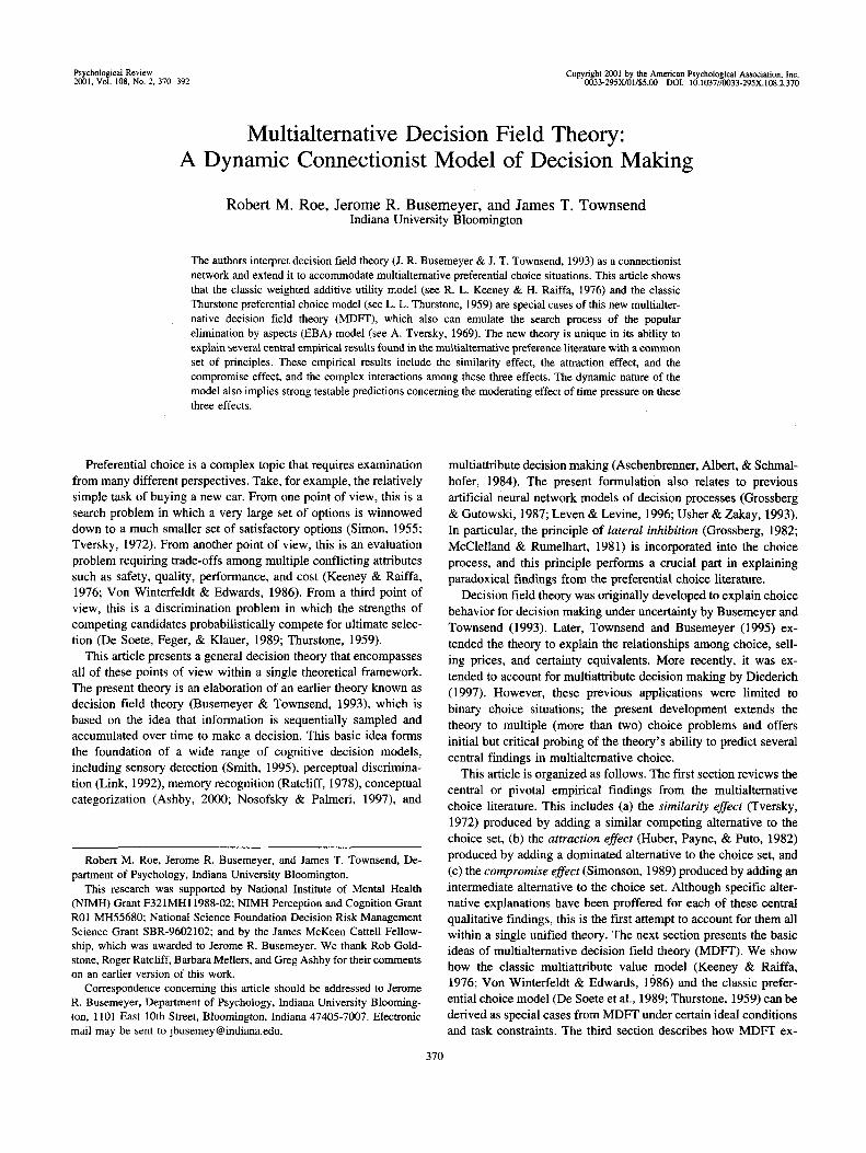
Consider the case of a new car purchase and suppose the choiceset has been reduced to a few cars, which differ primarily on onlytwo attributes, performance quality and driving economy. Figure 1presents a graphical depiction of the problem and clearly illustratesthe three major findings.
Similarity Effect
One of the first important results to arise from studies ofpreferential choice concerns the effect of adding a new competitiveoption to a choice set that already contains two dissimilar options
13
a
I
R
D
B
Driving Economy
Figure 1. A graphical .depiction of the problem of choosing between caroptions based on the two attributes of performance and economy. Thehorizontal axis represents the value of each car on the driving economyattribute, and the vertical axis represents the value of each car on theperformance quality attribute. Each car is then represented as a point in thistwo-dimensional space. For example, car A is high on quality and low oneconomy, whereas car B is low on quality and high on economy. Thesimilarity, attraction, and compromise effects can be illustrated clearlyusing this simple example.
(Sjoberg, 1977; Tversky, 1972). For example, suppose an industryconsiders the effect of introducing a new competitive product S ona market that already has two dissimilar competing products, Aand B. Furthermore, suppose the new product is highly similar toproduct A and dissimilar to the other product B. The main findingis that the introduction of the new competitive product to thechoice set reduces the probability of choosing similar productsmore than dissimilar products (Sjoberg, 1977; Tversky, 1972). Interms of market share, the new product steals more from similarproducts. This effect has significant practical implications formarketing and consumer research (Batsell & Polking, 1985; Bert-man, Johnson, & Payne, 1991; Lehmann & Pan, 1994).
Our three-car example in Figure 1 shows a similar situation. Thethree options are represented in a two-dimensional space of qualityand economy. Options A and B are located such that option A hasbetter quality but poorer economy than B, and option B has worsequality but better economy than A. Suppose the high-quality car Ais slightly more popular than the economical car B in a binarychoice (say 55% favor A over B). If another high-quality car S isintroduced, then it steals choices away from the original high-quality car A, evenly dividing the choices between A and S (27.5%each). However, the choices favoring the economical car B remainintact (45%), thus making it most popular in the trinary choice set.In general, a similarity effect occurs whenever the followingreversal of choice probabilities is obtained (Sjoberg, 1977; Tver-sky, 1972): Pr[A | {A, B}] > Pr[B | {A, B}] but Pr[A | {A, B, S}]< Pr[B {A, B, S}]. (Note: Pr[A | {A, B, S}] denotes theprobability of choosing option A from the set containing A, B,and S.)
The similarity effect produces violations of a preferential choiceproperty called independence from irrelevant alternatives. Accord-ing to this property, if x and y are both elements of a choice set T,which in turn is a subset of a larger choice set U, then PrOr 7] >Pr[y | T\ implies Pr[x | U] > Pr[y | U]. A large class of probabi-listic choice models, known as simple scalable utility models, mustsatisfy this property (Tversky, 1972). The simple scalable classincludes all models that assume that each alternative can be as-signed a utility scale value, independent of composition of thechoice set, and choice probability is determined from the utilitiesby the general formula Pr|> | T\ = F[u(x), «(y), . . . , u(z)], whereF is an increasing function of the first variable and a decreasingfunction of the all other variables. For example, Luce's (1959)well-known "ratio of strengths" choice model satisfies this prop-erty. The similarity effect violates the independence between ir-relevant alternatives property and rules out the entire class ofsimple scalable choice models.
Attraction Effect
A second important finding from studies of preferential choiceis the effect of adding a new option that is dominated by one of theother options in the original choice set (Huber, Payne, & Puto,1982; Ratneshwar, Shocker, & Stewart, 1987; Simonson, 1989;Wedell, 1991). For example, suppose an industry considers intro-ducing a new product D on a market that already has two highlydissimilar competitive products, A and B. Once again, the newproduct D is designed to be highly similar to an older product A,but in this case, A dominates D in the sense that A is better thanD on all the primary attributes. At the same time, D does not

372 ROE, BUSEMEYER, AND TOWNSEND
dominate B nor does B dominate D. In this case, D is called anasymmetrically dominated decoy. The attraction effect refers to thefact that the introduction of the new dominated product to a choiceset increases the probability of choosing the dominant product. Interms of market share, the new product enhances the market shareof the product that dominates it. (Note that this is the opposite ofthe similarity effect produced by a new competitive product.)
Figure 1 illustrates this choice situation for the car purchaseexample. As before, car A is superior on quality, whereas car B issuperior on economy. Car D is now slightly inferior on bothquality and economy as compared with car A. The attraction effectrefers to the empirical finding that adding D to the choice setincreases the probability that option A is chosen: Pr[A | {A, B}] <Pr[A | {A, B, D}].
The attraction effect produces a violation of a general principleimplied by a large class of random utility models called theregularity principle (cf. Colonius, 1984; MacKay & Zinnes, 1995;Marley, 1989). According to the regularity principle, for anyoption x that is an element of set W, which is in turn a subset of setU, x e W C U, the probability of choosing x from W must begreater than or equal to choosing x from U, Pr[x; W] ^ Pi[x; U].In other words, the addition of option D to the set already con-taining A and B should only decrease the probability that option Awill be chosen, not increase it. For example, the classic Thurstone(1959) preferential choice model must satisfy regularity, and theattraction effect rules out this entire class of models.
The regularity effect is rather robust. For example, Huber et al.(1982) investigated a variety of different choice conditions pro-ducing a wide range of binary choice probabilities. Adding thedominated decoy (D) increased the probability of choosing thedominant alternative (A) under all of these conditions. This in-cludes (a) when A was chosen less frequently than B in a binarychoice, (b) when A and B were chosen equally often in a binarychoice, and (c) when A was chosen more frequently than B in abinary choice.
Compromise Effect
A third important finding concerns the effect of adding a newoption that lies between two competing extreme options in theoriginal choice set (Simonson, 1989; Simonson & Tversky, 1992;Tversky & Simonson, 1993). Suppose there are three equallyattractive products, A, B, and C, as indicated by their pairwisepreferences, but suppose two of the products, say A and B, areextremely different, and the third product is a compromise that liesin between these two extremes. The compromise effect refers tothe empirical finding that when all three options are available forchoice, the compromise is chosen more frequently than either ofthe extremes. Unlike the previous decoy effect, the attractivenessof the compromise option is enhanced by introducing a newcompetitive (as opposed to dominated) option.
Figure 1 illustrates this choice situation for the car purchaseexample. As before, car A is superior on quality whereas car B issuperior on economy. Car C is a compromise lying in betweenthese two extremes—C is not as good as A on quality but betterthan A on economy, while C is not as good as B on economy butbetter than B on quality. The compromise effect refers to theempirical finding that Pr[A | {A, B}] = Pr[A {A, C}] = Pr[B |{B, C}], but Pr[C | {A, B, C}] > Pr[A | {A, B, C}] and Pr[C | {A,
B, C}] > Pr[B | {A, B, C}]. In other words, the compromise isenhanced when viewed within the context of the two extremes.Furthermore, the effect is found even when the trinary choice setis presented before the three binary comparisons (and thus theresult is not due to new information about options that changes theperception of attribute space used to describe the options).
Previous Explanations
Tversky (1972) developed the EBA model to explain the simi-larity effect. However, the EBA model also obeys the regularityprinciple (see Tversky, 1972), and therefore it is ruled out by theattraction effect. More recently, Tversky and Simonson (1993)proposed a context-dependent advantage model to account for theattraction and compromise effects. However, as proved in Appen-dix A, the context-dependent advantage model cannot account forthe similarity effect. Taken together, these three central findingscontinue to remain a deep puzzle for decision theorists. To date, nosingle theoretical explanation has been brought forth to explain allthree within a common theory.
Multialternative Decision Field Theory
The basic intuition underlying decision field theory is that adecision maker's preference for each option evolves during delib-eration by integrating a stream of comparisons of evaluationsamong options on attributes over time. Consider, for example, thecar purchase decision discussed earlier. Initially, the decisionmaker's attention may focus on the most important attribute (e.g.,quality) and some specific aspects (e.g., initial acceleration, con-trol on turns, stability at high speeds, stopping power) of thisattribute are evaluated for a period of time. During this timeperiod, the evaluation of each option is compared with others andthese comparisons change the preferences up or down dependingon whether an option has an advantage or disadvantage on theattended attribute. A few moments later, attention may switch toanother less important attribute (economy), and comparisons ofdetailed aspects (e.g., price, gas efficiency, repair costs, reliability,durability) related to this second attribute are added to the previouspreferences. Attention may then switch back to an earlier attributefor additional comparisons, and these comparisons continue toupdate the preferences for each option. Eventually a decision isreached either by an externally imposed time constraint (e.g., thecar dealer presses for a final decision) or by a self-imposedcriterion (e.g., preference exceeds a threshold and the buyer an-nounces a decision).
Multialternative Dynamic Decision Process
The decision process described above is an example of a largeclass of decision models called sequential sampling models (Link& Heath, 1975; Ratcliff, 1978; Vickers, 1979). Decision fieldtheory builds on this earlier theoretical work by extending theapplication of these models to multialternative preferential choicesituations. The sequential sampling decision process describedabove can be stated more formally, as follows.
Valences. At any moment in time, each alternative in thechoice set is associated with a valence value. The valence foroption i at time t, denoted w;(0. represents the momentary advan-
DYNAMIC MODEL OF DECISION MAKING 373
tage or disadvantage of option i when compared with other optionson some attribute under consideration. The ordered set of valencesfor all the options forms a valence vector, denoted \(t). Forexample, a choice among three alternatives {A, B, C} produces thethree-dimensional valence vector V(0 = [uA(0. %(')> %(?)]'• Thisvalence vector is determined by three different components.
The first component of valence is the personal evaluation ofeach option on each attribute. In general, the value m^ denotes thesubjective value of option i on attribute/ For example, consumer-oriented magazines or Web pages provide the reader with largematrices indicating the objective values of each option on a widevariety of attributes. Using this objective information, the readercan assess his or her personal or subjective evaluations (m'^s). Thegeneral model can accommodate any number of evaluations. Butfor the simplified car decision problem presented above, there areonly two primary attributes—economy and quality. The vectorME = [mAE, WBE, mCE]' represents the three evaluations for thethree cars on economy: If car A gets lower economy than car B,then mAE is assigned a lower scale value than mBE, so that mAE <mBE. Similarly, define MQ = [mAQ, mBQ, mcq]' as a vector ofevaluations for the three cars on quality: If car A has higher qualitythan car B, then mAQ is a assigned a higher scale value than mBQ,so that mAQ > mBQ. Concatenation of these two vectors forms a3 X 2 value matrix, M = [ME | MQ].
The second component of valence is the attention weight allo-cated to each attribute at a particular moment in time. The mo-mentary attention to attribute j is represented by an attentionweight, Wj(f), at time t. For example, consumer-oriented maga-zines or Web pages facilitate evenhanded attention to a widevariety of attributes, allowing the reader to rely on his or her ownjudgments regarding the importance or relevance to the decision.Magazine, television, or Web advertisements attempt to manipu-late or draw the viewer's attention to particular attributes that favorthe sponsor's product. The general model can accommodate anynumber of attributes, but for the simplified car purchase example,there are only two attention weights, WE(f) for economy, and WQ(I)for quality. The attention weights vary from moment to momentdue to changes and fluctuations in attention to the attributes overtime. For example, at one moment in time, the decision maker mayfocus on one attribute (e.g., acceleration), but at later moment,attention may switch to another attribute (e.g., rising cost of gas).In general, the attention weights change and fluctuate across timeaccording to a stationary process. For the present application, it issufficient to assume that attention shifts in an all-or-none mannerfrom one attribute at one moment, Wq(f) = 1, WE(t) = 0, toanother attribute at another moment, WQ(t + 1) = 0, WE(t +1) = 1, with some fixed probabilities. The probability of attendingto the economic dimension is denoted WE, and the probability ofattending to the quality dimension is denoted WQ. This implies anexponential waiting time for attention to shift from one givenattribute to another.1 The attention weights for all of the attributesform a weight vector W(f). For the car purchase example with onlytwo attributes (quality and economy), the weight vector is a two-dimensional vector W(r) = [WE(t)WQ(t)]'.
The matrix product of weights and values, MW(f), determinesthe weighted value of each alternative at each time point. Forexample, when choosing among three cars, the j'th row of theproduct MW(f) equals the weighted value of ith option: WE(r)m,E+ WQ(f)m/Q. At first glance, this looks like the classic weighted
utility model. However, unlike the classic weighted utility modelthese weighted values are stochastic because of fluctuations in theattention weights WE(t) and WQ(t). A static version of this randomweight utility model was successfully used by Fischer, Jia, andLuce (2000) to explain inconsistencies in ratings obtained frommultiattribute judgment research.
The third and final component used to determine the valences ofeach option is the comparison process that contrasts the weightedevaluations of each option. This comparison process is needed todetermine the relative advantage or disadvantage of each option onthe attribute being considered at that moment. In general, thevalence for each option is produced by contrasting the weightedvalue of one alternative against the average of all the others. Forexample, with three alternatives, {A, B, C}, the valence for optionA is computed by the contrast vA(t) = WE(f)'MAE + WQ(O»»AQ —l(WE(t)mBE + WQ(t)mBQ) + (WE(t)mCE + WQ(t)mCQ)]/2. Thiscomparison process also can be represented by a matrix operationby defining a contrast matrix:
C =1 - 1/2 - V2 '
Using this matrix definition, the valence vector is formed by thematrix product
V(r) = CMW(r). (la)
Each row of the matrix product produces a valence or comparisonvalue similar to that shown for option A.
The car purchase example described above contains for simplic-ity, only three alternatives described by two primary attributes.However, most decisions involve a larger number of attributes, andEquation la is applicable with arbitrary numbers of alternativesand attributes. However, in practice it is useful to group thepossibly large number of attributes into two subgroups, a relativelysmall subgroup of primary attributes of importance and a largersubgroup of irrelevant attributes. For example, the experimentsdiscussed later usually design the options by manipulating a fewprimary dimensions, but these options may also differ on a numberof other irrelevant attributes. Even in these more complex settings,a simplified analysis can be performed by partitioning ap-dimensional attention weight vector into two components W(f)'= [Wj(f)', W2(r)'], where W^r) is a ^-dimensional componentcontaining the primary dimensions and W2(f) contains the remain-ing p-q irrelevant dimensions. Then Equation la can be rewrittenin terms of the primary and irrelevant dimensions as follows:
V(r) = CMW(r) = + e(f), (Ib)
where e(f) = CM2W2(f) can be treated as an stochastic error orresidual term.
Preferences. At any moment in time, each alternative in thechoice set is associated with a preference strength. The preference
1 In this application we assume that the attention weights are identicallyand independently distributed over time according to a simple Bernoulliprocess. However, Diederich's (1997) multiattribute decision field modelemploys a more sophisticated Markov process for switching attention toattributes. The Bernoulli process is a simple special case of the moregeneral Markov process, but it is sufficient for the present purposes.

374 ROE, BUSEMEYER, AND TOWNSEND
strength for alternative / at time t, denoted P,(f)> represents theintegration of all the valences considered for alternative i up to thatpoint in time. The preferences for all the alternatives form apreference state vector, denoted P(f). For example, a choice amongthree options {A, B, C} produces the three-dimensional preferencestate P(0 = [PA(t), PB(f), Pc(t)]'.
A new state of preference P(t + 1) is formed at each momentfrom the previous preference state P(f) and the new input valencevector, V(f), according to the following linear stochastic differenceequation:
P(t+ 1) = SP(r) + V(r+ 1). (2)
According to this simple updating equation, the new preferencestate is a weighted combination of the previous preference stateand the new input valence. The dynamic behavior of this model isdetermined by two factors: the initial preference state P(0) at timet = 0, and the feedback matrix S.
Initial preference state. In general, the initial preference staterepresents a residual bias left over from previous experience withchoice problems. For example, status quo effects (Samuelson &Zeckhauser, 1988), previous habits, or experience and memory forthe previous history of choices can be captured by the initial state.For novel choice problems, the initial state may be consideredunbiased, in which case P(0) = 0. The applications presentedbelow are based on the latter assumption.
Feedback matrix. The feedback matrix S shown in Equa-tion 2 contains the self-connections and interconnections amongthe choice alternatives. The diagonal elements, Su, determinethe memory of the previous preference state for a given alter-native. These self-feedback loops are needed to integrate thevalences for a given option over time, and they allow thepreference strength within an alternative to grow or decay overtime. If the self-feedback loop is set to zero, then that option hasno memory of its previous state. If the .strength of the self-connection is set to one, then that option has perfect memory ofits previous state. Intermediate strengths, between zero and one,provide partial memory and limited decay. For the presentwork, the self-feedback loops are identical for all options, thatis, S,, is the same for all i.
The off-diagonal elements, Sy for i =£ j, determine the influenceof one alternative on another. These interconnections are generallynegative so that they produce competitive influences. If the inter-connections are all zero, then the alternatives do not compete at alland instead they grow or decay independently and in parallel. If theinterconnections are negative, then strong alternatives suppressweak alternatives. The strengths of the interconnections are deter-mined by the concept of lateral inhibition (discussed again in thesection on connectionist networks). The basic idea is that thestrength of the lateral interconnection between a pair of options isa decreasing function of the distance between these two options inthe multiattribute space.
More formally, it is assumed that each alternative is representedas a point in a multidimensional space with dimensions defined bythe attributes used to characterize the choice alternatives. Forexample, Figure 1 illustrates a small set of cars placed within atwo-dimensional space characterized by quality and economy. Inthis example, Options A and B are highly dissimilar, and two otheroptions, S and D, are both highly similar to option A. Thus pairs(A, S) and (A, R) have much stronger inhibitory interconnections
than pairs (A, B), (S, B), or (R, B). Define dtj as the psychologicaldistance between options i and./ in this multiattribute preferencespace. Then the interconnection between options i and j is deter-mined by Sy = F[d(Ai, A,)], where F is a decreasing function. Atthis point we do not need to specify the form of F (e.g., exponentialis one possibility; see Shepard, 1964). But this equation does placetwo important constraints on the lateral inhibition connections:One is symmetry, StJ = Sjt, and the second is that the interconnec-tion decreases with distance.
Conceptually, options that are unrelated to each other elicit littleor no competition, whereas options that are closely related producegreater competition. These interconnections provide a dynamicmechanism for producing bolstering effects (Janis & Mann, 1977)and justification effects (Simonson, 1989) in preference. When aweak unattractive alternative is compared with a strong attractivealternative, the negative values from the weak option feed backthrough a negative connection and the product of these two factorsproduces a net positive effect that bolsters or justifies the strongoption.
Multiattribute utility model. If the feedback matrix is set tozero (S = 0), then according to Equation 2, the preference stateequals the valence input, P(f) = V(t). If it is also assumed thatattention does not fluctuate across time, Yf(t) = w, and theresiduals in Equation Ib are zero, e(t) = 0, then valence V =CMw produces exactly the same rank order as classic multiat-tribute weighted additive values (Keeney & Raiffa, 1976; VonWinterfeldt & Edwards, 1986). Applying the car purchase exampleto this special case, the valence for option A reduces to VA =
2. Furthermore, VA > Max^, vc) implies that (w^m^ +Max[(wEmBE + WQ/MBQ), (wEmCE + WQ/WCQ)]. Thus, V producesexactly the same rank order over alternatives as the classic multi-attribute model under these restrictive conditions.
Dynamic Thurstone model. On the basis of the multivariatecentral limit theorem, the distribution of the preference states P(f)converges to the multivariate normal distribution as the number ofsteps (t) in Equation 2 becomes large. If the time period betweensteps is small, then this convergence will occur very rapidly. If thefeedback matrix S is set equal to an identity matrix (all cross-feedback set to zero), at any fixed time point t. Equation 2 reducesto a multivariate Thurstone preferential choice model (Bock &Jones, 1968; see Appendix B for details). Note that MDFT is adynamic generalization of the classic Thurstone preference model,as it describes how the mean vector and variance- covariancematrix of the preference state evolve systematically over time.2
The mean preferences for each alternative can change signs overtime so that initially one alternative (say A) may have the largestmean preference, but later another alternative (say C) may come todominate.
Summary of parameters. Altogether there are four sets ofparameters that need to be specified to derive predictions from
2 Previous theorists working in sensory, perception, and memory haveshown that unidimensional sequential sampling models provide generali-zations of the unidimensional signal detection models (Link and Heath,1975; Ratcliff, 1978). The present work extends these ideas to preferentialchoice and provides a generalization of the multivariate Thurstone modelincluding arbitrary variance—covariance structures.
DYNAMIC MODEL OF DECISION MAKING 375
MDFT. Two sets of parameters are contained in the mean weightand value matrices, w and M, which are also required by theclassic multiattribute utility model. A third parameter is the resid-ual variance contributed by the irrelevant attributes, which is alsorequired by any Thurstone-type probabilistic choice model. Thefinal set is contained in the symmetric feedback matrix, S, whichis required by any dynamic connectionist model. The parameters inthe S matrix are a function of the distance between alternatives inthe attribute space. In the case of three alternatives, the feedbackmatrix produces at most three new parameters (self-feedback, A toB inhibition, and A to C inhibition).
Multialternative Choice Rules
Eventually, the evolving output preferences, P(r), determine thefinal choice. But the specific decision rule for determining thischoice varies depending on whether the decision time is externallyimposed versus subject controlled, as described next.
Externally controlled stopping time. Choice tasks are termedexternally controlled when the decision is made at an appointedtime or designated time point (Ratcliff, 1978; Vickers, Smith, &Brown, 1985). For example, a woman who has just received aproposal for marriage may be asked to announce her decision atbreakfast the next morning. Alternatively, a woman who has justbeen offered a job may be asked to sign her contract by the end ofthe week. For the car choice example, the car dealer, on seeingother customers waiting for help, may lose his patience, interruptthe purchaser, and pressure her to make an immediate decision.
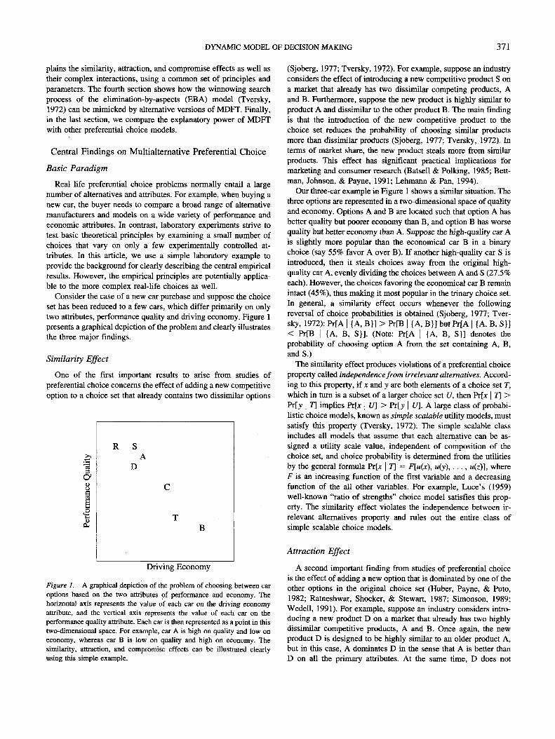
The vertical line in Figure 2 illustrates this type of stopping rulefor the new car example. In this case, the option with the highestpreference at the designated time point is chosen (option B inFigure 2).
Formally, the probability that one alternative (say A) is chosenfrom a set of three alternatives {A, B, C} at a fixed time t isdetermined by the relation:
Pr[A | {A, B, C} at time t\ =
Pr[PA(r) and Pc(t)]. (3)
Determination of choice probabilities for choice sets with N alter-natives follows the same principle outlined in Equation 3, exceptthat it requires the conjunction ofN-l events of the form PA(t)>Pt(t), for i =£ A. Appendix B provides the mathematical formulasfor calculating probabilities using Equation 3.
By stopping the deliberation process at various designated timepoints and estimating the choice probabilities as a function ofdeliberation time, it is possible to observe the evolution of pref-erences dynamically over time. Cognitive researchers have usedthis type of paradigm to study the dynamics of memory (Dosher,1984; Gronlund & Ratcliff, 1989; Hintzman & Curran, 1997;Ratcliff, 1978; Ratcliff, 1980; Ratcliff & McKoon, 1982; Ratcliff& McKoon, 1989; Reed, 1973; Wickelgren, Corbett, & Dosher,1980). Although this method has not been applied to preferentialchoice, the present theory provides simple predictions for this typeof task. These predictions will be presented later during the reviewof the empirical results for preferential choice. The second type ofchoice task is presented next.
200 300Deliberation Time
400 500
Figure 2. Illustration of the two stopping rules. The abscissa repre-sents time, and the ordinate represents level of preference. The threetrajectories (labeled A, B, and C) represent the preferences of eachoption as they evolve stochastically over time. The vertical line tothe left represents the appointed time for the decision according tothe externally controlled stopping rule. In this case, option B wouldbe chosen at the designated time t = 150. The horizontal line on thetop represents the inhibitory threshold that must be reached tomake a choice for the subject-controlled stopping rule. In this case,option A would be chosen when it crosses the threshold at timet = 430.
Internally controlled stopping time. Choice tasks are calledinternally controlled decisions when the decision maker is free todecide how long to deliberate before finally announcing or com-mitting to a particular choice (Ratcliff, 1978; Vickers et al., 1985).In the car purchase example, the buyer may inform the car dealerthat she wishes to go home and think about the purchase and thatshe will call back as soon as she makes up her mind. This is acommon type of choice task used in laboratory experiments ondecision making.
The horizontal line in Figure 2 illustrates this type of stoppingrule for the new car example. In this case, a choice is made as soonas the strength of preference for an option crosses a threshold, andthe first option to exceed the threshold is then chosen (option A inthe figure).
The choice probabilities and decision times for the internallycontrolled task are determined by the first passage time distribu-tion for a sample path to cross the threshold boundary (see Bhat-tacharya & Waymire, 1990; Cox and Miller, 1965; Smith, 2000).Formulas for computing the first passage time distribution (as wellas the moments including choice probabilities and mean decisiontimes) have been derived by Busemeyer and Townsend (1992) andby Diederich (1997) for the binary choice case and by Busemeyerand Diederich (2000) for more than two options. Alternatively, thefirst passage time distribution for the multichoice (more than two)case can be obtained through computer simulation (see AppendixC for details).
376 ROE, BUSEMEYER, AND TOWNSEND
Connectionist Interpretation
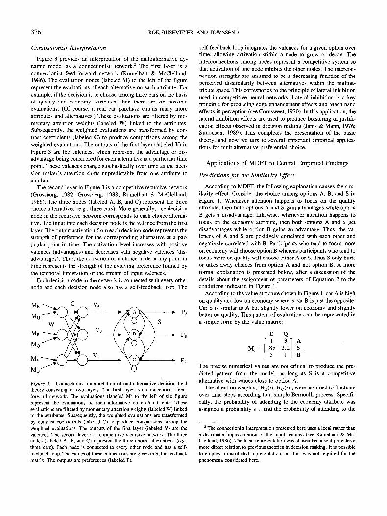
Figure 3 provides an interpretation of the multialternative dy-namic model as a connectionist network.3 The first layer is aconnectionist feed-forward network (Rumelhart & McClelland,1986). The evaluation nodes (labeled M) to the left of the figurerepresent the evaluations of each alternative on each attribute. Forexample, if the decision is to choose among three cars on the basisof quality and economy attributes, then there are six possibleevaluations. (Of course, a real car purchase entails many moreattributes and alternatives.) These evaluations are filtered by mo-mentary attention weights (labeled W) linked to the attributes.Subsequently, the weighted evaluations are transformed by con-trast coefficients (labeled C) to produce comparisons among theweighted evaluations. The outputs of the first layer (labeled V) inFigure 3 are the valences, which represent the advantage or dis-advantage being considered for each alternative at a particular timepoint. These valences change stochastically over time as the deci-sion maker's attention shifts unpredictably from one attribute toanother.
The second layer in Figure 3 is a competitive recursive network(Grossberg, 1982; Grossberg, 1988; Rumelhart & McClelland,1986). The three nodes (labeled A, B, and C) represent the threechoice alternatives (e.g., three cars). More generally, one decisionnode in the recursive network corresponds to each choice alterna-tive. The input into each decision node is the valence from the firstlayer. The output activation from each decision node represents thestrength of preference for the corresponding alternative at a par-ticular point in time. The activation level increases with positivevalences (advantages) and decreases with negative valences (dis-advantages). Thus, the activation of a choice node at any point intime represents the strength of the evolving preference formed bythe temporal integration of the stream of input valences.
Each decision node in the network is connected with every othernode and each decision node also has a self-feedback loop. The
*• PC
Figure 3. Connectionist interpretation of multialternative decision fieldtheory consisting of two layers. The first layer is a connectionist feed-forward network. The evaluations (labeled M) to the left of the figurerepresent the evaluations of each alternative on each attribute. Theseevaluations are filtered by momentary attention weights (labeled W) linkedto the attributes. Subsequently, the weighted evaluations are transformedby contrast coefficients (labeled C) to produce comparisons among theweighted evaluations. The outputs of the first layer (labeled V) are thevalences. The second layer is a competitive recursive network. The threenodes (labeled A, B, and C) represent the three choice alternatives (e.g.,three cars). Each node is connected to every other node and has a self-feedback loop. The values of these connections are given in S, the feedbackmatrix. The outputs are preferences (labeled P).
self-feedback loop integrates the valences for a given option overtime, allowing activation within a node to grow or decay. Theinterconnections among nodes represent a competitive system sothat activation of one node inhibits the other nodes. The intercon-nection strengths are assumed to be a decreasing function of theperceived dissimilarity between alternatives within the multiat-tribute space. This corresponds to the principle of lateral inhibitionused in competitive neural networks. Lateral inhibition is a keyprinciple for producing edge enhancement effects and Mach bandeffects in perception (see Cornsweet, 1970). In this application, thelateral inhibition effects are used to produce bolstering or justifi-cation effects observed in decision making (Janis & Mann, 1976;Simonson, 1989). This completes the presentation of the basictheory, and now we turn to several important empirical applica-tions for multialternative preferential choice.
Applications of MDFT to Central Empirical Findings
Predictions for the Similarity Effect
According to MDFT, the following explanation causes the sim-ilarity effect. Consider the choice among options A, B, and S inFigure 1. Whenever attention happens to focus on the qualityattribute, then both options A and S gain advantages while optionB gets a disadvantage. Likewise, whenever attention happens tofocus on the economy attribute, then both options A and S getdisadvantages while option B gains an advantage. Thus, the va-lences of A and S are positively correlated with each other andnegatively correlated with B. Participants who tend to focus moreon economy will choose option B whereas participants who tend tofocus more on quality will choose either A or S. Thus S only hurtsor takes away choices from option A and not option B. A moreformal explanation is presented below, after a discussion of thedetails about the assignment of parameters of Equation 2 to theconditions indicated in Figure 1.
According to the value structure shown in Figure 1, car A is highon quality and low on economy whereas car B is just the opposite.Car S is similar to A but slightly lower on economy and slightlybetter on quality. This pattern of evaluations can be represented ina simple form by the value matrix:
M, =
E Q1 3
.85 3.23 1
ASB
The precise numerical values are not critical to produce the pre-dicted pattern from the model, as long as S is a competitivealternative with values close to option A.
The attention weights, tWE(r), WQ(0], were assumed to fluctuateover time steps according to a simple Bernoulli process. Specifi-cally, the probability of attending to the economy attribute wasassigned a probability WB, and the probability of attending to the
3 The connectionist interpretation presented here uses a local rather thana distributed representation of the input features (see Rumelhart & Mc-Clelland, 1986). The local representation was chosen because it provides amore direct relation to previous theories in decision making. It is possibleto employ a distributed representation, but this was not required for thephenomena considered here.
DYNAMIC MODEL OF DECISION MAKING 377
quality attribute was assigned a probability WQ, with independentsampling across time steps (but see Footnote 1). The probability ofattending to the quality attribute was set to a slightly higher level(WQ = .45) than the probability of attending to the economyattribute (WE = .43), and there was some small residual probabilityallowed for attention to irrelevant attributes. The reason for theslight difference in attention to each attribute was to produce aslight preference in favor of car A over car B for the binary choicecondition. This was needed to satisfy the antecedent condition forthe test of independence from irrelevant alternatives. These sameparameters were then used to make new predictions for the trinarychoice set.
The parameters for the feedback matrix were chosen as follows.First, the self-connections were set to a high value (Su = .94) toproduce slow decay of memory. The inhibitory connections be-tween distant alternatives were set to very low values (SAB =SBA = SSB = SBS = —.001). The inhibitory connections betweenthe similar alternatives were set to relatively greater magnitudes(SAS = SSA = —.025). These parameter values satisfy a stabilityrequirement (i.e., the eigenvalues of the feedback matrix S are allless than 1 in magnitude). The predicted pattern does not changemuch as long as the inhibitory connections are not too large.
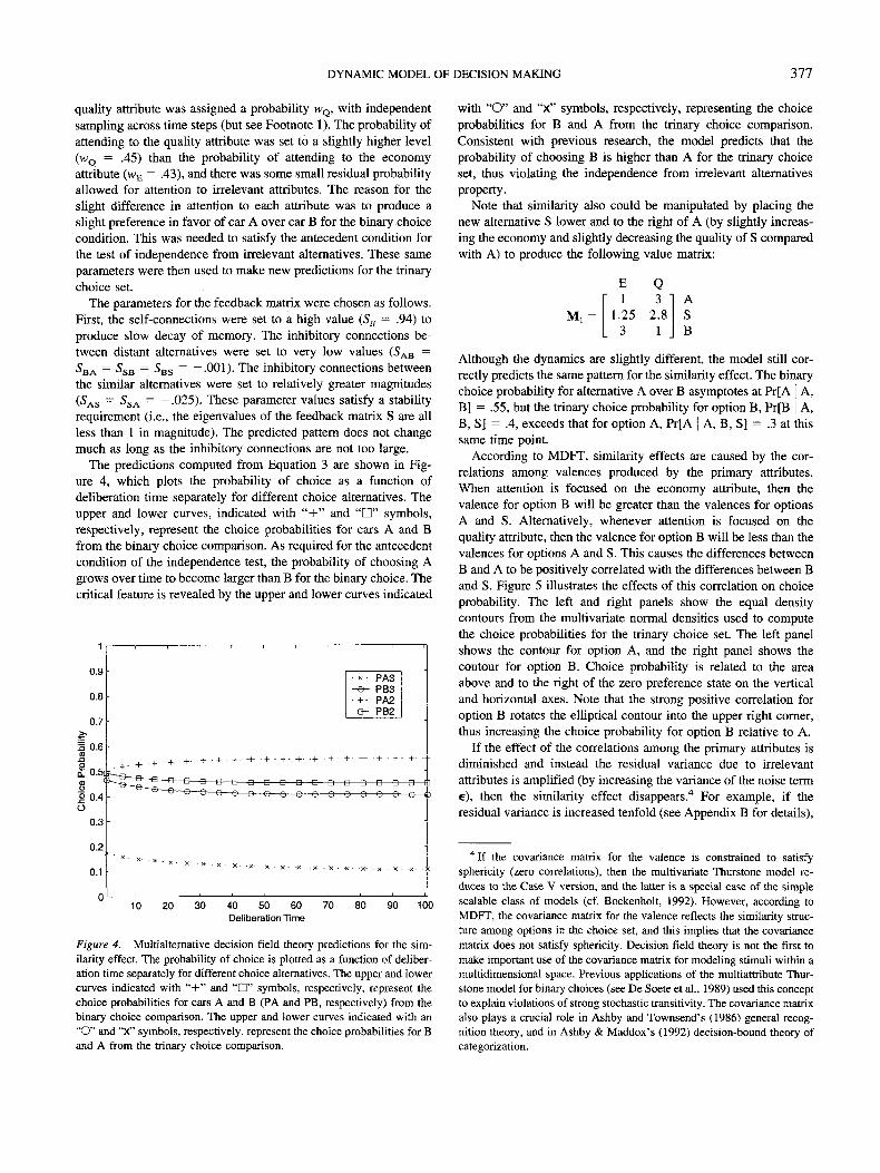
The predictions computed from Equation 3 are shown in Fig-ure 4, which plots the probability of choice as a function ofdeliberation time separately for different choice alternatives. Theupper and lower curves, indicated with "+" and "D" symbols,respectively, represent the choice probabilities for cars A and Bfrom the binary choice comparison. As required for the antecedentcondition of the independence test, the probability of choosing Agrows over time to become larger than B for the binary choice. Thecritical feature is revealed by the upper and lower curves indicated
10 20 30 40 50 60 70 80 90 100Deliberation Time
Figure 4. Multialternative decision field theory predictions for the sim-ilarity effect. The probability of choice is plotted as a function of deliber-ation time separately for different choice alternatives. The upper and lowercurves indicated with "+" and "D" symbols, respectively, represent thechoice probabilities for cars A and B (PA and PB, respectively) from thebinary choice comparison. The upper and lower curves indicated with an"O" and "x" symbols, respectively, represent the choice probabilities for Band A from the trinary choice comparison.
with "O" and "x" symbols, respectively, representing the choiceprobabilities for B and A from the trinary choice comparison.Consistent with previous research, the model predicts that theprobability of choosing B is higher than A for the trinary choiceset, thus violating the independence from irrelevant alternativesproperty.
Note that similarity also could be manipulated by placing thenew alternative S lower and to the right of A (by slightly increas-ing the economy and slightly decreasing the quality of S comparedwith A) to produce the following value matrix:
M,=
choice probability for alternative A over B asymptotes at Pr[AB] = .55, but the trinary choice probability for option B, Pr[B
Although the dynamics are slightly different, the model still cor-rectly predicts the same pattern for the similarity effect. The binary
A,A,
B, S] = .4, exceeds that for option A, Pr[A | A, B, S] = .3 at thissame time point.
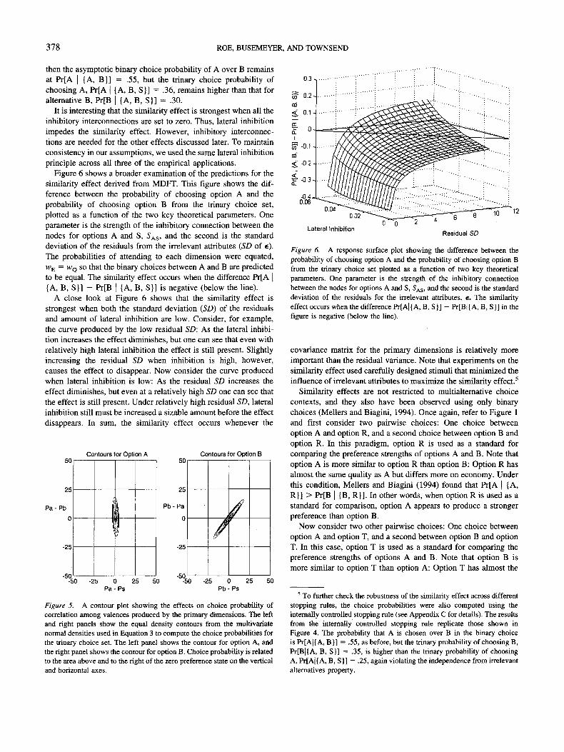
According to MDFT, similarity effects are caused by the cor-relations among valences produced by the primary attributes.When attention is focused on the economy attribute, then thevalence for option B will be greater than the valences for optionsA and S. Alternatively, whenever attention is focused on thequality attribute, then the valence for option B will be less than thevalences for options A and S. This causes the differences betweenB and A to be positively correlated with the differences between Band S. Figure 5 illustrates the effects of this correlation on choiceprobability. The left and right panels show the equal densitycontours from the multivariate normal densities used to computethe choice probabilities for the trinary choice set. The left panelshows the contour for option A, and the right panel shows thecontour for option B. Choice probability is related to the areaabove and to the right of the zero preference state on the verticaland horizontal axes. Note that the strong positive correlation foroption B rotates the elliptical contour into the upper right corner,thus increasing the choice probability for option B relative to A.
If the effect of the correlations among the primary attributes isdiminished and instead the residual variance due to irrelevantattributes is amplified (by increasing the variance of the noise terme), then the similarity effect disappears.4 For example, if theresidual variance is increased tenfold (see Appendix B for details),
4 If the covariance matrix for the valence is constrained to satisfysphericity (zero correlations), then the multivariate Thurstone model re-duces to the Case V version, and the latter is a special case of the simplescalable class of models (cf. Bockenholt, 1992). However, according toMDFT, the covariance matrix for the valence reflects the similarity struc-ture among options in the choice set, and this implies that the covariancematrix does not satisfy sphericity. Decision field theory is not the first tomake important use of the covariance matrix for modeling stimuli within amultidimensional space. Previous applications of the multiattribute Thur-stone model for binary choices (see De Soete et al., 1989) used this conceptto explain violations of strong stochastic transitivity. The covariance matrixalso plays a crucial role in Ashby and Townsend's (1986) general recog-nition theory, and in Ashby & Maddox's (1992) decision-bound theory ofcategorization.
378 ROE, BUSEMEYER, AND TOWNSEND
then the asymptotic binary choice probability of A over B remainsat Pr[A | {A, B}] = .55, but the trinary choice probability ofchoosing A, Pr[A | {A, B, S}] = .36, remains higher than that foralternative B, Pr[B | {A, B, S}] = .30.
It is interesting that the similarity effect is strongest when all theinhibitory interconnections are set to zero. Thus, lateral inhibitionimpedes the similarity effect. However, inhibitory interconnec-tions are needed for the other effects discussed later. To maintainconsistency in our assumptions, we used the same lateral inhibitionprinciple across all three of the empirical applications.
Figure 6 shows a broader examination of the predictions for thesimilarity effect derived from MDFT. This figure shows the dif-ference between the probability of choosing option A and theprobability of choosing option B from the trinary choice set,plotted as a function of the two key theoretical parameters. Oneparameter is the strength of the inhibitory connection between thenodes for options A and S, SAS, and the second is the standarddeviation of the residuals from the irrelevant attributes (SD of e).The probabilities of attending to each dimension were equated,WE = WQ so that the binary choices between A and B are predictedto be equal. The similarity effect occurs when the difference Pr[A |(A, B, S}] - Pr[B | {A, B, S}] is negative (below the line).
A close look at Figure 6 shows that the similarity effect isstrongest when both the standard deviation (SD) of the residualsand amount of lateral inhibition are low. Consider, for example,the curve produced by the low residual SD: As the lateral inhibi-tion increases the effect diminishes, but one can see that even withrelatively high lateral inhibition the effect is still present. Slightlyincreasing the residual SD when inhibition is high, however,causes the effect to disappear. Now consider the curve producedwhen lateral inhibition is low: As the residual SD increases theeffect diminishes, but even at a relatively high SD one can see thatthe effect is still present. Under relatively high residual SD, lateralinhibition still must be increased a sizable amount before the effectdisappears. In sum, the similarity effect occurs whenever the
Contours for Option A Contours for Option B
25
Pa-Pb
0
-25
-50s
1)
0 -25 0 25 5Pa -Ps
25
Pb-Pa
0
-25
-500 -5
t
/P
/
0 -25 0 25 5Pb-Ps
Figure 5. A contour plot showing the effects on choice probability ofcorrelation among valences produced by the primary dimensions. The leftand right panels show the equal density contours from the multivariatenormal densities used in Equation 3 to compute the choice probabilities forthe trinary choice set. The left panel shows the contour for option A, andthe right panel shows the contour for option B. Choice probability is relatedto the area above and to the right of the zero preference state on the verticaland horizontal axes.
-0.40.06
0.04
Lateral InhibitionResidual SD
Figure 6. A response surface plot showing the difference between theprobability of choosing option A and the probability of choosing option Bfrom the trinary choice set plotted as a function of two key theoreticalparameters. One parameter is the strength of the inhibitory connectionbetween the nodes for options A and S, 5AS, and the second is the standarddeviation of the residuals for the irrelevant attributes, e. The similarityeffect occurs when the difference Pr[A|{A, B, S}] - Pr[B|{A, B, S}] in thefigure is negative (below the line).
covariance matrix for the primary dimensions is relatively moreimportant than the residual variance. Note that experiments on thesimilarity effect used carefully designed stimuli that minimized theinfluence of irrelevant attributes to maximize the similarity effect.5
Similarity effects are not restricted to multialtemative choicecontexts, and they also have been observed using only binarychoices (Mellers and Biagini, 1994). Once again, refer to Figure 1and first consider two pairwise choices: One choice betweenoption A and option R, and a second choice between option B andoption R. In this paradigm, option R is used as a standard forcomparing the preference strengths of options A and B. Note thatoption A is more similar to option R than option B: Option R hasalmost the same quality as A but differs more on economy. Underthis condition, Mellers and Biagini (1994) found that Pr[A | {A,R}] > Pr[B | {B, R}]. In other words, when option R is used as astandard for comparison, option A appears to produce a strongerpreference than option B.
Now consider two other pairwise choices: One choice betweenoption A and option T, and a second between option B and optionT. In this case, option T is used as a standard for comparing thepreference strengths of options A and B. Note that option B ismore similar to option T than option A: Option T has almost the
5 To further check the robustness of the similarity effect across differentstopping rules, the choice probabilities were also computed using theinternally controlled stopping rule (see Appendix C for details). The resultsfrom the internally controlled stopping rule replicate those shown inFigure 4. The probability that A is chosen over B in the binary choiceis Pr[A|{A, B}] = .55, as before, but the trinary probability of choosing B,Pr[B|{A, B, S}] = .35, is higher than the trinary probability of choosingA, Pr[A|{A, B, S)] = .25, again violating the independence from irrelevantalternatives property.
DYNAMIC MODEL OF DECISION MAKING 379
same quality as B but differs more on economy. Under thiscondition, Mellers and Biagini (1994) found Pr[B {B, T}] > Pr[A| {A, T}]. In other words, when option T is used as a standard forcomparison, option B appears to produce a stronger preferencethan option A. This reversal in binary choice probabilities consti-tutes another type of violation of independence between alterna-tives. This violation rules out all simple scalable utility models forbinary choices (Tversky, 1972).
MDFT predicts these results using exactly the same parametersas used in Figure 4, except for changes in the value matrices:
M,= M,=
E" 12.53
Q3 "
1.11
ATB
The asymptotic predictions derived from Equation 3 reproduce theviolation of independence observed by Mellers & Biagini (1994):Pr[A | {A, R}] = .99 > Pr[B | {B, R}] = .63; Pr[B | {B, T}] =.99 > Pr[A {A, T}] = .77. These predictions are robust withrespect to lateral inhibition: The same result is obtained with
SAR = = -.025 and with 5AR = 5BT = 0.The intuitive reason for this predicted pattern is simple to
explain. First consider the choice between options A and R: Whenattention is focused on quality, little difference in valence occurs,but when attention is focused on economy, a large positive valencefavoring option A occurs. Next consider the choice between op-tions B and R: When attention is focused on quality, large valencesfavoring option R occur, but when attention is focused on econ-omy, large valences favoring B occur. Analogously, when choos-ing between B and T, the valence almost always favors B, butwhen choosing between A and T, valences oscillate back and forth,one moment favoring A, the next moment favoring T. Technically,binary choice probability is determined by the ratio of the meandifference and the standard deviation of the difference (see Ap-pendix B). The variance of the preference difference is larger forthe choice between dissimilar (e.g., B and R) as compared tosimilar (e.g., A and R) options.
So far we have shown that MDFT can reproduce the well-known similarity effect under a wide variety of conditions whenthe valences on the primary attributes are correlated in a mannerthat reflects the similarity structure in the choice set. But severalearlier choice models were developed to explain these results(EBA model of Tversky, 1972, and the multivariate Thurstonemodel of Edgell & Geisler, 1980, for multiple choice; Mellers &Biagini, 1994, for binary choice). The next challenge is faced bysimultaneously explaining the similarity effect as well as theattraction effect. All of the above mentioned multiple-choice mod-els satisfy a general property known as the regularity principle.The attraction effect described next produces empirical violationsof the regularity principle.
Predictions for the Attraction Effect
According to MDFT, the following explanation causes the at-traction effect. Consider a choice among options A, B, and D inFigure 1 . Comparisons of the dominated decoy with the average ofthe other two options eventually produces a negative preferencestate for the dominated decoy, D. Then this negative preferencestate from the dominated decoy feeds through a negative inhibitory
link to the closely positioned dominant option, A. The two nega-tives cancel to produce a net positive bolstering effect of thedominated decoy on the dominant option. Thus the decoy makesthe dominant option "appear" stronger, similar to an edge enhance-ment effect in perception. Option B does not experience anybolstering effect because it is too dissimilar to D, and the inhibitoryconnection is too weak to produce the effect. A more formalanalysis is provided below.
The only change in assignment of parameters that needs to bemade for computing the predictions from Equation 3 for theattraction effect is the value matrix M (which is necessary torepresent the new location of dominated option D in Figure 1). Allof the remaining parameters were kept constant across the twodifferent applications.
According to the value structure shown in Figure 1, car A is highon quality and low on economy whereas car B is just the opposite.Car D is similar to A but slightly inferior on economy and quality.This pattern of evaluations can be represented in a simple form bythe value matrix
M, =
Once again, the precise numerical values are not critical to producethe predicted pattern from the model. For example, very similarresults are obtained when the values of D are set to (.75, 2.75)instead of (.5, 2.5).
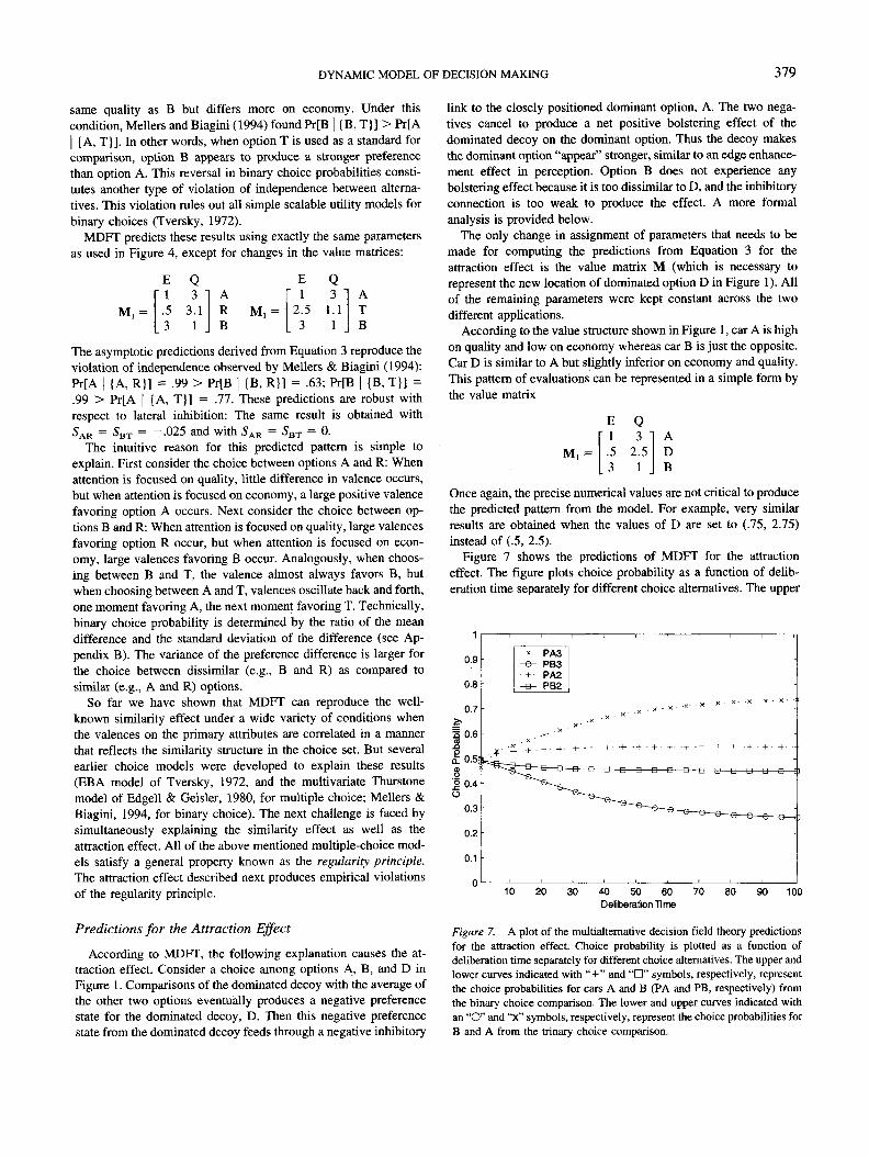
Figure 7 shows the predictions of MDFT for the attractioneffect. The figure plots choice probability as a function of delib-eration time separately for different choice alternatives. The upper
10 20 30 40 50 60 70 80 90 100Deliberation Time
Figure 7. A plot of the multialternative decision field theory predictionsfor the attraction effect. Choice probability is plotted as a function ofdeliberation time separately for different choice alternatives. The upper andlower curves indicated with "+" and "D" symbols, respectively, representthe choice probabilities for cars A and B (PA and PB, respectively) fromthe binary choice comparison. The lower and upper curves indicated withan "O" and "x" symbols, respectively, represent the choice probabilities forB and A from the trinary choice comparison.

380 ROE, BUSEMEYER, AND TOWNSEND
and lower curves indicated with "+" and "D" symbols, respec-tively, represent the choice probabilities for cars A and B from thebinary choice set. Similar to Figure 4, the probability of choosingA grows over time to become larger than B for the binary choice.The upper and lower curves, indicated with "x" and "O" symbols,respectively, represent the choice probabilities for A and B fromthe trinary choice set. Consistent with previous research, the modelcorrectly predicts that the probability of choosing A is higher fromthe trinary choice set (the "x" curve) as compared to the proba-bility of choosing A from the binary choice set (the "+" curve),thus violating the regularity property.
To check the robustness of this prediction, it was recomputedusing Equation 3 after changing the probabilities attending to eachof the primary attributes. In one case, the probability of attendingto each attribute was equated (WE = WQ = .45), producing binarychoice probabilities equal to .50 for A and B, but the probability ofchoosing A from the trinary set rose to .69. In another case, theywere reversed (WB = .43, WQ = .45), producing a binary choiceprobability equal to .45 for option A, but once again the probabilityof choosing A from the trinary set rose to .65. In both cases, thesame pattern of predictions was obtained for the dominating alter-native—the decoy increased the predicted probability of choosingthe dominating alternative (i.e., adding D increased the probabilityof choosing A) in agreement with results from Huber et al. (1982).
Note that Figure 7 was generated using exactly the same modelparameters as Figure 4, except for the change in the M matrix toreflect the change of option D from a competitive to a dominatedalternative close to option A. But the predicted effect of adding thedominated option (Figure 7) was just the opposite of the predictedeffect of adding the competitive option (Figure 4). The theoreticalreason for this dramatic change in predictions needs to be under-stood. If the lateral inhibitory connections are set to zero so that thefeedback matrix S is set equal to a diagonal matrix, then theattraction effect disappears. In this case, the predictions computedfrom Equation 3 produced the following results: The decoy D isvirtually ignored, the probability of choosing A from the binaryand trinary choice sets remain identical and both equaled .55, andthe decoy has no effect on the dominating alternative A.
It turns out that the correlations among the primary attributes donot play a crucial role for the attraction effect. Figure 8 shows thepredictions when the lateral inhibition is reset to its original value(as used in Figure 7), but the effect of the residual variances (SDof e) is increased tenfold. As can be seen in Figure 8, the attractioneffect still occurs, although now it takes some time to build up. Insum, lateral inhibitory connections are crucial and covariancestructure is less important for MDFT to produce the attractioneffect.
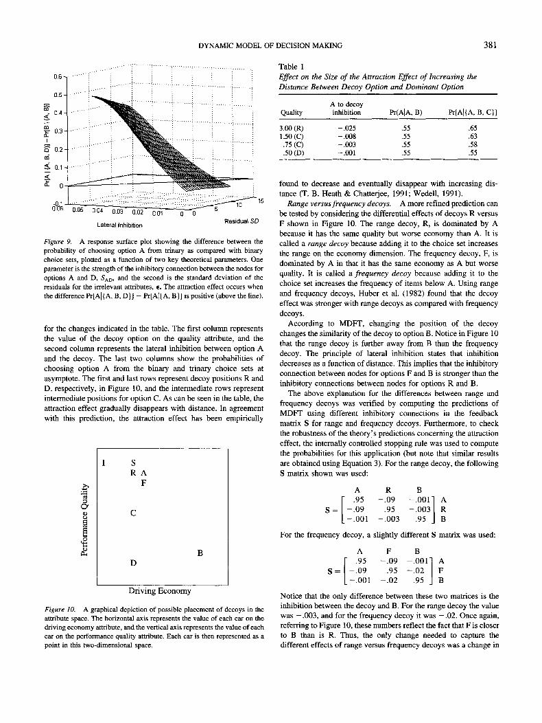
Figure 9 shows a more detailed examination of the predictionsfor the attraction effect derived from MDFT. This figure shows thedifference between the probability of choosing option A from thetrinary set and the probability of choosing A from the binary set,plotted as a function of the two key theoretical parameters: thestrength of the inhibitory connection between the nodes for optionsA and D, 5AD, and the standard deviation of the residuals for theirrelevant attributes, SD of e. The probabilities of attending to eachdimension were equated, WE = WQ so that the binary choicesbetween A and B are predicted to be equal. The attraction effectoccurs when the difference Pr[A | {A, B, D}] - Pr[A | {A, B}] ispositive (above the line).
1
0.9
0.8
0.7
.£15 0.6
IX 0.5
1° 0.4O
0.3
0.2
0.1
0
-e—a—a—a—a—a—a—B-
20 40 60Deliberation Time
SO 100
Figure 8. A plot of the multialternative decision field theory predictionsfor the attraction effect when the influence of the diagonal matrix ofresidual variances is increased tenfold. The upper and lower curves indi-cated with "+" and "D" symbols, respectively, represent the choiceprobabilities for cars A and B (PA and PB, respectively) from the binarychoice comparison. The lower and upper curves indicated with "O" and"x" symbols, respectively, represent the choice probabilities for B and Afrom the trinary choice comparison.
A close look at Figure 9 shows that the attraction effect isstrongest when the SD of the residuals is low and amount of lateralinhibition is high. Consider, for example, the curve produced bythe low residual SD: As the lateral inhibition increases, the effectquickly becomes present and increases dramatically with increas-ing amounts of lateral inhibition. Now consider the curve producedwhen lateral inhibition is low: When the residual SD is low, theeffect is not present, and increasing residual SD does not lead tothe occurrence of the effect. In sum, lateral inhibition is muchmore critical to explaining the attraction effect than is amount ofresidual SD.
A complete explanation for similarity and attraction effects mustinclude a formal explanation for their intricate interactions. Thenext section considers the effects of systematically varying theposition of the decoy on similarity and attraction effects.
Similarity and Attraction Interactions
Distance effects. A fundamental implication of the lateral in-hibitory explanation for the attraction effect is that it shoulddiminish with psychological distance between the decoy and thedominant option. Refer to Figure 10, and consider moving thedecoy from position R through C and straight down the qualityattribute to position D. According to MDFT, this movement in-creases the distance between the decoy and dominant option,causing the lateral inhibition between the decoy and the dominantoption to decrease. MDFT predicts that the bolstering effect of thedecoy should eventually be eliminated after moving from positionsR through C to D.
Table 1 illustrates this effect, where the results are computedfrom Equation 3 using the same parameters as in Figure 7, except
DYNAMIC MODEL OF DECISION MAKING 381
0.05 Q.C4 0.03" Q.OT 0.01
Lateral InhibitionResidual SD
Figure 9. A response surface plot showing the difference between theprobability of choosing option A from trinary as compared with binarychoice sets, plotted as a function of two key theoretical parameters. Oneparameter is the strength of the inhibitory connection between the nodes foroptions A and D, 5AD, and the second is the standard deviation of theresiduals for the irrelevant attributes, e. The attraction effect occurs whenthe difference Pr[A]{A, B, D)] - Pr[A|( A, B}] is positive (above the line).
for the changes indicated in the table. The first column representsthe value of the decoy option on the quality attribute, and thesecond column represents the lateral inhibition between option Aand the decoy. The last two columns show the probabilities ofchoosing option A from the binary and trinary choice sets atasymptote. The first and last rows represent decoy positions R andD, respectively, in Figure 10, and the intermediate rows representintermediate positions for option C. As can be seen in the table, theattraction effect gradually disappears with distance. In agreementwith this prediction, the attraction effect has been empirically
•8
sR
BD
Driving Economy
Figure 10. A graphical depiction of possible placement of decoys in theattribute space. The horizontal axis represents the value of each car on thedriving economy attribute, and the vertical axis represents the value of eachcar on the performance quality attribute. Each car is then represented as apoint in this two-dimensional space.
Table 1Effect on the Size of the Attraction Effect of Increasing theDistance Between Decoy Option and Dominant Option
Quality
3.00 (R)1.50 (C).75 (C).50(0)
A to decoyinhibition
-.025-.008-.003-.001
Pr(A|A, B)
.55
.55
.55
.55
Pr[A|(A, B, C}]
.65
.63
.58
.55
found to decrease and eventually disappear with increasing dis-tance (T. B. Heath & Chatterjee, 1991; Wedell, 1991).
Range versus frequency decoys. A more refined prediction canbe tested by considering the differential effects of decoys R versusF shown in Figure 10. The range decoy, R, is dominated by Abecause it has the same quality but worse economy than A. It iscalled a range decoy because adding it to the choice set increasesthe range on the economy dimension. The frequency decoy, F, isdominated by A in that it has the same economy as A but worsequality. It is called a frequency decoy because adding it to thechoice set increases the frequency of items below A. Using rangeand frequency decoys, Huber et al. (1982) found that the decoyeffect was stronger with range decoys as compared with frequencydecoys.
According to MDFT, changing the position of the decoychanges the similarity of the decoy to option B. Notice in Figure 10that the range decoy is further away from B than the frequencydecoy. The principle of lateral inhibition states that inhibitiondecreases as a function of distance. This implies that the inhibitoryconnection between nodes for options F and B is stronger than theinhibitory connections between nodes for options R and B.
The above explanation for the differences between range andfrequency decoys was verified by computing the predictions ofMDFT using different inhibitory connections in the feedbackmatrix S for range and frequency decoys. Furthermore, to checkthe robustness of the theory's predictions concerning the attractioneffect, the internally controlled stopping rule was used to computethe probabilities for this application (but note that similar resultsare obtained using Equation 3). For the range decoy, the followingS matrix shown was used:
S =
A.95
-.09.001
For the frequency decoy, a slightly different S matrix was used:
A F BT .95 -.09 -.001] A
S= -.09 .95 -.02 FL-.001 -.02 .95 J B
Notice that the only difference between these two matrices is theinhibition between the decoy and B. For the range decoy the valuewas -.003, and for the frequency decoy it was -.02. Once again,referring to Figure 10, these numbers reflect the fact that F is closerto B than is R. Thus, the only change needed to capture thedifferent effects of range versus frequency decoys was a change in

382 ROE, BUSEMEYER, AND TOWNSEND
lateral inhibition that reflects the distances of the objects in at-tribute space.
Figure 11 shows the predictions of MDFT under various choiceconditions for range and frequency decoys. Each point in the figurerepresents a pair of probabilities, Pr[A | {A, B}], Pr[A | {A, B, C}],obtained from the same choice condition. In Figure 11, the regu-larity principle requires all of the points to lie on or below theidentity line. Violations of regularity occur when any of the pointsappear above the identity line. As can be seen in Figure 11, themodel predicts that adding either a frequency or a range decoyproduces violations of regularity across the entire range of binarychoice probabilities. Furthermore, the range decoy has a largereffect as compared with the frequency decoy, consistent with thefindings of Huber et al. (1982).
Inferior decoys. A final test MDFT is obtained by consideringthe effect of adding what is called an inferior decoy to the choiceset. For example, consider the decoy labeled "I" in Figure 10.Technically, this is a competitive option because it is superior tooption A on quality. Practically, however, it is inferior to option Abecause the small advantage in terms of quality is offset by a largedisadvantage in terms of economy. Inferior decoys are like dom-inated decoys in the sense that they are rarely ever chosen. Huberand Puto (1983) examined the effects of inferior decoys and foundthat they produced attraction effects similar to dominated decoys.
Note that if option I shown in Figure 10 is shifted horizontallyover to the right toward the position of option S in Figure 10, then
0.8-
0.4-
0.2-
-Rangedecoy-Frequencydecoy
0 0.2 0.4 0.6 0.8 1
Pr(Choose A) - Binary
Figure 11. A plot showing results from multialternative decision fieldtheory under various choice conditions for range and frequency decoys.The abscissa represents the probability that the dominating option (A) ischosen from a binary choice set. The ordinate represents the probabilitythat A is chosen out of a trinary choice set that includes a decoy. Each pointin the figure represents a pair of probabilities (Pr), Pr[A|{A, B}], Pr[A|{A,B, C}], obtained from the same choice condition. The line connected bysolid circles represents the probability that A is chosen when the frequencydecoy was presented for various choice conditions. The line connected bythe solid triangles represents the probability that A is chosen when therange decoy was presented for various choice conditions. The diagonalidentity line represents the separation of where the attraction effect doesand does not occur. Any points above the line represent areas where theeffect does occur and below where it does not.
the inferior option changes into a highly competitive option. Huberand Puto (1983) also examined the effect of gradually changing theinferior option into a competitive option in this manner. Theyfound that the proportion of choices for option A decreased, theproportion of choices for option I increased, but the proportion ofchoices for option B changed very little. In other words, bothattraction and similarity effects were demonstrated within the samestudy.
These interactions are precisely the effects expected fromMDFT. Table 2 shows the results at asymptote computed fromEquation 3 using the same parameters as used to produce Figures 4and 7, except for changes in the value of economy for the inferioroption. The first column shows the gradual shifts in the value ofthe economy attribute from .85 (i.e., the value used to defineoption S in Figure 10) to .55 (i.e., the value used to define optionI in Figure 10). The second and third rows show the probabilitiesof choosing options A and B from the trinary choice set {A, B, I}.As can be seen in the table, decreasing the economy drasticallyincreased the probability of choosing option A, while the proba-bility for B changed very little. Also note that an attraction effectis produced by the inferior option when the economy was very lowin value. These predictions are in accord with the findings byHuber and Puto (1983).
Although earlier choice models have been proposed specificallyto account for the attraction effect (e.g., Ariely & Wallsten, 1995;Dhar & Glazer, 1996), only MDFT has been simultaneously ap-plied to both the similarity and attraction effects and their inter-actions. Furthermore, these earlier models never attempted toformally explain another finding known as the compromise effectdescribed next.
Predictions for the Compromise Effect
The compromise effect presents a real challenge for MDFTbecause no special mechanisms were built into the theory toproduce this effect. Nevertheless, the same mechanisms thatMDFT used to explain the similarity and attraction effect worktogether to produce the compromise effect.
The experimental conditions used to produce the compromiseeffect required a few changes in model parameters. First, thevalues in the matrix M were changed to represent the new locationof compromise option C in Figure 1 as follows. According to thevalue structure shown in Figure 1, car A is high on quality and lowon economy whereas car B is just the opposite. Car C is in betweenthese two, being inferior to B on economy and inferior to A onquality. This pattern of evaluations can be represented in a simpleform by the value matrix:
M
Once again, the precise numerical values are not critical to producethe predicted pattern from the model as long as the compromiseposition indicated in the matrix is satisfied.
The inhibitory connections in the feedback matrix also need tobe changed to reflect the equal distances between the compromiseoption and the two extreme options. The self-connections were setto Sti = .94 (as before), the inhibitory connections between the two

DYNAMIC MODEL OF DECISION MAKING 383
extreme options were set to SAB = SBA = -.001 (as before), andthe inhibitory connections between the compromise and eachextreme were set to SAC = SCA = 5CB = 5BC = -.025. Note thatall these parameters are exactly the same as those used to producethe attraction effect in Figure 8. The only difference is that theinhibitory connections between A and C are now set to the samevalues as the inhibitory connections between C and B, reflectingthe fact that the compromise is placed in between the twoextremes.
Finally, the probability of attending to the quality attribute wasset equal to the probability of attending to the economy dimension(WE = wQ = .45). This was necessary to meet the antecedentconditions for the compromise effect. Using these parametersforced all of the binary choice probabilities equal to .50. Theremaining model parameters used to compute the predictions fromEquation 3 were assigned exactly the same values as those used toproduce the attraction effect shown in Figure 8.
Figure 12 shows the predictions of MDFT for the compromiseeffect. The figure plots choice probability as a function of delib-eration time separately for different choice alternatives. The uppercurve indicated with a "+" symbol represents the choice proba-bility for the compromise car C out of the binary choice set. Theoverlapping two lower curves represent the choice probabilities forthe two extreme options, A and B, from the trinary choice set. Thechoice probabilities from the binary choice set are not shownbecause all three are exactly equal (.50). Figure 12 shows that theprobability of choosing the complement alternative, C, grows overtime to become larger than both A and B. Consistent with previousresearch, the model correctly predicts that the probability of choos-ing the compromise from the trinary set is higher than the ex-tremes, despite the fact that the binary choice probabilities are allequal.6
Once again, lateral inhibition is crucial for producing this effect.If the lateral inhibitory interconnections are eliminated, then thepredicted compromise effect disappears. But the explanation isquite different from that used to explain the attraction effect.Lateral inhibition does not bolster the mean preference of thecompromise alternative because all three options are assignedequally attractive weighted values. The mean valence input is zerofor all, and multiplication of the feedback matrix, S, by the zeromean input produces zero mean output, and thus the mean pref-erence state remains at zero over time.
Table 2Effect of Inferior Option on Trinary Choice Probabilities
Economy for I Pr[A|(A, B, I}] Pr[B|{A, B, I}]
.85
.75
.65
.55
.33
.50
.57
.61
.43
.42
.40
.38
Note. The first column refers to the value of the M matrix correspondingto the first attribute, economy, for the inferior option I. The first rowcorresponds to the position of option S in Figure 10, and the last rowcorresponds to the position of option I in Figure 10. The second and thirdrows correspond to positions of inferior alternatives shifted horizontallyalong the line from I to S. The binary choice probability of choosing A overB was uniformly equal to .55 for all rows.
0.2540 60Deliberation Time
Figure 12. Predictions of multialternative decision field theory for thecompromise effect. Choice probability is plotted as a function of deliber-ation time separately for different choice alternatives. The upper curveindicated with a "+" symbol represents the choice probability for thecompromise car C (PCS) out of the trinary choice set. The overlapping twolower curves represent the choice probabilities for the two extreme options,car A (PA3) and car B (PBS), from the trinary choice set.
The source of the effect lies in the operation of lateral inhibitionon the momentary fluctuations in valence. The negative inhibitoryconnections between the nodes for the compromise and extremeoptions cause the compromise to be negatively correlated withboth of the extremes. This in turn causes the differences betweenthe compromise and extreme option A to be positively correlatedwith the difference between the compromise and extreme option B.Finally, the positive correlation for the compromise provides aprobabilistic advantage over the extreme option in Equation 3.
The probabilistic advantage produced by the positive correlationcan be seen in Figure 13. The left and right panels show the equaldensity contours from the multivariate normal densities used inEquation 3 to compute the choice probabilities for the trinarychoice set. The left panel shows the contour for an extreme option(e.g., A), and the right panel shows the contour for the compromiseoption C. Choice probability is related to the area above and to theright of the zero preference state on the vertical and horizontalaxes. Note that the relatively stronger positive correlation for thecompromise rotates the elliptical contour further into the upperright corner, thus increasing the choice probability for the com-promise option.
At this point, we can examine one of the most important issuesconcerning the explanation of the similarity, attraction, and com-
6 To check the robustness of the predictions for MDFT, the predictionswere computed again using the internally controlled stopping rule andslightly different parameters (see Appendix C for details). The parameterswere assigned in a manner to guarantee that all three binary choiceprobabilities were equal to .50. The results for the trinary choice setproduced the same pattern of results as shown in Figure 12: The probabilityof choosing the compromise (.48) exceeded the probability of choosingeither the upper extreme option A (.27) or the lower extreme option B (.25).
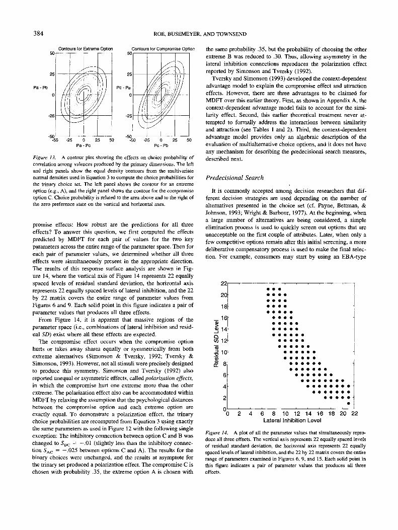
384 ROE, BUSEMEYER, AND TOWNSEND
50
25
Contours for Extreme Option Contours for Compromise Option
Pa-Pb
-25
-50-50 -25 25 50 -50
Pa-Pc-25 0 25
Pc-Pb
Figure 13. A contour plot showing the effects on choice probability ofcorrelation among valences produced by the primary dimensions. The leftand right panels show the equal density contours from the multivariatenormal densities used in Equation 3 to compute the choice probabilities forthe trinary choice set. The left panel shows the contour for an extremeoption (e.g., A), and the right panel shows the contour for the compromiseoption C. Choice probability is related to the area above and to the right ofthe zero preference state on the vertical and horizontal axes.
promise effects: How robust are the predictions for all threeeffects? To answer this question, we first computed the effectspredicted by MDFT for each pair of values for the two keyparameters across the entire range of the parameter space. Then foreach pair of parameter values, we determined whether all threeeffects were simultaneously present in the appropriate direction.The results of this response surface analysis are shown in Fig-ure 14, where the vertical axis of Figure 14 represents 22 equallyspaced levels of residual standard deviation, the horizontal axisrepresents 22 equally spaced levels of lateral inhibition, and the 22by 22 matrix covers the entire range of parameter values fromFigures 6 and 9. Each solid point in this figure indicates a pair ofparameter values that produces all three effects.
From Figure 14, it is apparent that massive regions of theparameter space (i.e., combinations of lateral inhibition and resid-ual SD) exist where all these effects are expected.
The compromise effect occurs when the compromise optionhurts or takes away shares equally or symmetrically from bothextreme alternatives (Simonson & Tversky, 1992; Tversky &Simonson, 1993). However, not all stimuli were precisely designedto produce this symmetry. Simonson and Tversky (1992) alsoreported unequal or asymmetric effects, called polarization effects,in which the compromise hurt one extreme more than the otherextreme. The polarization effect also can be accommodated withinMDFT by relaxing the assumption that the psychological distancesbetween the compromise option and each extreme option areexactly equal. To demonstrate a polarization effect, the trinarychoice probabilities are recomputed from Equation 3 using exactlythe same parameters as used in Figure 12 with the following singleexception: The inhibitory connection between option C and B waschanged to SBC = — .01 (slightly less than the inhibitory connec-tion 5AC = —.025 between options C and A). The results for thebinary choices were unchanged, and the results at asymptote forthe trinary set produced a polarization effect. The compromise C ischosen with probability .35, the extreme option A is chosen with
the same probability .35, but the probability of choosing the otherextreme B was reduced to .30. Thus, allowing asymmetry in thelateral inhibition connections reproduces the polarization effectreported by Simonson and Tversky (1992).
Tversky and Simonson (1993) developed the context-dependentadvantage model to explain the compromise effect and attractioneffects. However, there are three advantages to be claimed forMDFT over this earlier theory. First, as shown in Appendix A, thecontext-dependent advantage model fails to account for the simi-larity effect. Second, this earlier theoretical treatment never at-tempted to formally address the interactions between similarityand attraction (see Tables 1 and 2). Third, the context-dependentadvantage model provides only an algebraic description of theevaluation of multialternative choice options, and it does not haveany mechanism for describing the predecisional search measures,described next.
Predecisional Search
It is commonly accepted among decision researchers that dif-ferent decision strategies are used depending on the number ofalternatives presented in the choice set (cf. Payne, Bettman, &Johnson, 1993; Wright & Barbour, 1977). At the beginning, whena large number of alternatives are being considered, a simpleelimination process is used to quickly screen out options that areunacceptable on the first couple of attributes. Later, when only afew competitive options remain after this initial screening, a moredeliberative compensatory process is used to make the final selec-tion. For example, consumers may start by using an EBA-type
22
20
18
16
J 1 4
I 12
8 ftcc 8
6
4
2
0 2 4 6 8 10 12 14 16 18 20 22Lateral Inhibition Level
Figure 14. A plot of all the parameter values that simultaneously repro-duce all three effects. The vertical axis represents 22 equally spaced levelsof residual standard deviation, the horizontal axis represents 22 equallyspaced levels of lateral inhibition, and the 22 by 22 matrix covers the entirerange of parameters examined in Figures 6, 9, and 15. Each solid point inthis figure indicates a pair of parameter values that produces all threeeffects.

DYNAMIC MODEL OF DECISION MAKING 385
choice rule (Tversky, 1972) and then later switch to a weightedadditive difference rule (Tversky, 1969).
A large amount of evidence has accumulated over the past 20years for strategy-switching dependent on choice set size (seePayne et al., 1993). One index used to monitor strategies is theproportion of information searched, defined as the ratio of thenumber of cells considered out of the total the number of cellsavailable within an alternative by attribute value matrix. This indexhas been found to decrease as the choice set size increases.Another important index is the direction of search, defined as theratio (between-attribute comparisons — within-attribute compari-sons)/(within-attribute comparisons + between-attribute compari-sons). This index has been found to decrease in the negativedirection favoring more within-attribute comparisons as the choiceset size increases. Both of these findings are consistent with theidea of strategy-switching from a more thorough compensatoryprocess to a quick elimination process as the choice set sizeincreases. Other process measures based on eye movements andmemory recall of values also support this general idea (see I. P.Levin & Jasper, 1995; Russo & Rosen, 1975).
In this section, we show how MDFT mimics strategy-switchingsimply by adding a second lower elimination boundary to theinternally controlled stopping rule (an idea first proposed by Rat-cliff, 1978). Previous applications of the internally controlledstopping rule considered only the case where there was an upperacceptance boundary. Now consider the case where there is only alower rejection boundary and no upper acceptance boundary. Fig-ure 15 illustrates an example for a hypothetical deliberation pro-cess involving five new cars that are evaluated along three at-tributes. The abscissa represents time and the ordinate representspreference. The lower reject boundary is placed at —50 in thefigure. Each line represents the evolution of preferences computedfrom Equation 2 for a particular car option over time. The verticallines represent shifts of attention from one attribute to anotherduring the deliberation process. In this case, the first attribute iseconomy, the second comfort, and the third quality. As can beseen, while focusing on the first attribute, economy, two of theoptions (B, E) were eliminated from the choice set. With the shift
Economy Comfort Performance
Boundary todiscard
Time
Figure 15. An illustration of the essential ideas for a hypothetical delib-eration process involving five new cars that are evaluated along threeattributes. The abscissa represents time and the ordinate represents prefer-ence. Each line represents the evolution of preferences for a particular caroption over time. The vertical lines represent shifts of attention from oneattribute to another during the deliberation process. The first attribute iseconomy, the second comfort, and the third quality.
to the second attribute, comfort, no items were eliminated. How-ever, with the shift to the third attribute, quality, two more options(C, D) were eliminated. Finally, the choice is based on the lastremaining option (A).
The complete version of this decision process uses both anupper acceptance boundary and a lower rejection boundary. Thelower boundary represents the criterion level of preference used toreject options from consideration. The upper boundary representsthe criterion level of preference used to select an option as the finalchoice. But in this case, there are two ways an option can bechosen: One is to be the first to cross the upper boundary (stoppingthe search), and if that fails for all options then the other is to bethe last to survive rejection.
The double-boundary version of MDFT can mimic strategy-switching by allowing the lower reject boundary to change de-pending on the number of options initially presented to the deci-sion maker. When the choice set is large, the lower boundary is setequal to a small distance below the neutral point (zero preferencestate), thus allowing quick rejection of inferior alternatives andonly allowing superior alternatives to survive further consider-ation. When the choice set is small, then the lower boundary is setfarther below the neutral point to avoid eliminating any option tooquickly and every alternative receives thorough consideration. Ingeneral, the criterion for rejecting becomes more lenient (closer toneutral) as the choice set size increases.
To show how this simple idea mimics strategy-switching phe-nomena, a simulation was performed using the choice sets pre-sented in one of the original predecisional processing studies byPayne, Braunstein, and Carroll (1978). In this study, participantswere presented 2, 7, or 12 alternatives described by 12 attributes,with one of three (low, medium, or high) evaluations assigned toeach alternative-attribute cell. Furthermore, the alternatives wereconstructed so that each alternative was high on four attributes,medium on four, and low on four, and the distribution variedacross alternatives so that no alternative dominated another.
One thousand simulated decision makers were run on the abovemultiple-choice task using Equation 2 to generate the preferencesand double boundaries to make the final decision (see Appendix Cfor details). The criterion for rejection was set to high, medium,and low magnitudes for the 2, 7, and 12 alternative choice sets,respectively. The main results for this simulation are shown inFigure 16. The steeply declining curve shows the results producedby the 12-alternative choice set, the flat curve shows the results forthe 2-alternative choice set, and the intermediate curve shows theresults for the 7-alternative choice set.
For the 12-alternative set, the majority of options are rejectedvery quickly on the basis of comparisons within only the first orsecond attributes. For example, the probability of rejecting any oneof the 12 options on the basis of the first attribute is .45, and theprobability of rejecting an option on second attribute (given that itsurvived the first attribute) is .40. On the average, 8 out of 12alternatives are eliminated on the basis of the first two attributesalone. But as the number of attributes processed in increases, theprobability of rejection rapidly declines, so that the probability ofrejecting any one of the superior options that survives until theseventh attribute is only .10 and this rejection probability graduallyapproaches zero. Thus the double-boundary model behaves like anelimination process when a large number of alternatives are avail-able in the choice set.
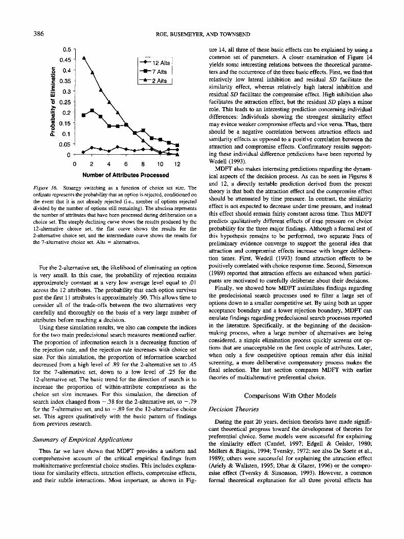
386 ROE, BUSEMEYER, AND TOWNSEND
2 4 6 8
Number of Attributes Processed
Figure 16. Strategy switching as a function of choice set size. Theordinate represents the probability that an option is rejected, conditioned onthe event that it is not already rejected (i.e., number of options rejecteddivided by the number of options still remaining). The abscissa representsthe number of attributes that have been processed during deliberation on achoice set. The steeply declining curve shows the results produced by the12-alternative choice set, the flat curve shows the results for the2-alternative choice set, and the intermediate curve shows the results forthe 7-alternative choice set. Alts = alternatives.
For the 2-alternative set, the likelihood of eliminating an optionis very small. In this case, the probability of rejection remainsapproximately constant at a very low average level equal to .01across the 12 attributes. The probability that each option survivespast the first 11 attributes is approximately .90. This allows time toconsider all of the trade-offs between the two alternatives verycarefully and thoroughly on the basis of a very large number ofattributes before reaching a decision.
Using these simulation results, we also can compute the indicesfor the two main predecisional search measures mentioned earlier.The proportion of information search is a decreasing function ofthe rejection rate, and the rejection rate increases with choice setsize. For this simulation, the proportion of information searcheddecreased from a high level of .89 for the 2-alternative set to .45for the 7-alternative set, down to a low level of .25 for the12-alternative set. The basic trend for the direction of search is toincrease the proportion of within-attribute comparisons as thechoice set size increases. For this simulation, the direction ofsearch index changed from —.38 for the 2-altemative set, to —.79for the 7-alternative set, and to -.89 for the 12-alternative choiceset. This agrees qualitatively with the basic pattern of findingsfrom previous research.
Summary of Empirical Applications
Thus far we have shown that MDFT provides a uniform andcomprehensive account of the critical empirical findings frommultialternative preferential choice studies. This includes explana-tions for similarity effects, attraction effects, compromise effects,and their subtle interactions. Most important, as shown in Fig-
ure 14, all three of these basic effects can be explained by using acommon set of parameters. A closer examination of Figure 14yields some interesting relations between the theoretical parame-ters and the occurrence of the three basic effects. First, we find thatrelatively low lateral inhibition and residual SD facilitate thesimilarity effect, whereas relatively high lateral inhibition andresidual SD facilitate the compromise effect. High inhibition alsofacilitates the attraction effect, but the residual SD plays a minorrole. This leads to an interesting prediction concerning individualdifferences: Individuals showing the strongest similarity effectmay evince weaker compromise effects and vice versa. Thus, thereshould be a negative correlation between attraction effects andsimilarity effects as opposed to a positive correlation between theattraction and compromise effects. Confirmatory results support-ing these individual difference predictions have been reported byWedell (1993).
MDFT also makes interesting predictions regarding the dynam-ical aspects of the decision process. As can be seen in Figures 8and 12, a directly testable prediction derived from the presenttheory is that both the attraction effect and the compromise effectshould be attenuated by time pressure. In contrast, the similarityeffect is not expected to decrease under time pressure, and insteadthis effect should remain fairly constant across time. Thus MDFTpredicts qualitatively different effects of time pressure on choiceprobability for the three major findings. Although a formal test ofthis hypothesis remains to be performed, two separate lines ofpreliminary evidence converge to support the general idea thatattraction and compromise effects increase with longer delibera-tion times. First, Wedell (1993) found attraction effects to bepositively correlated with choice response time. Second, Simonson(1989) reported that attraction effects are enhanced when partici-pants are motivated to carefully deliberate about their decisions.
Finally, we showed how MDFT assimilates findings regardingthe predecisional search processes used to filter a large set ofoptions down to a smaller competitive set. By using both an upperacceptance boundary and a lower rejection boundary, MDFT canemulate findings regarding predecisional search processes reportedin the literature. Specifically, at the beginning of the decision-making process, when a large number of alternatives are beingconsidered, a simple elimination process quickly screens out op-tions that are unacceptable on the first couple of attributes. Later,when only a few competitive options remain after this initialscreening, a more deliberative compensatory process makes thefinal selection. The last section compares MDFT with earliertheories of multialternative preferential choice.
Comparisons With Other Models
Decision Theories
During the past 20 years, decision theorists have made signifi-cant theoretical progress toward the development of theories forpreferential choice. Some models were successful for explainingthe similarity effect (Candel, 1997; Edgell & Geisler, 1980;Mellers & Biagini, 1994; Tversky, 1972; see also De Soete et al.,1989); others were successful for explaining the attraction effect(Ariely & Wallsten, 1995; Dhar & Glazer, 1996) or the compro-mise effect (Tversky & Simonson, 1993). However, a commonformal theoretical explanation for all three pivotal effects has
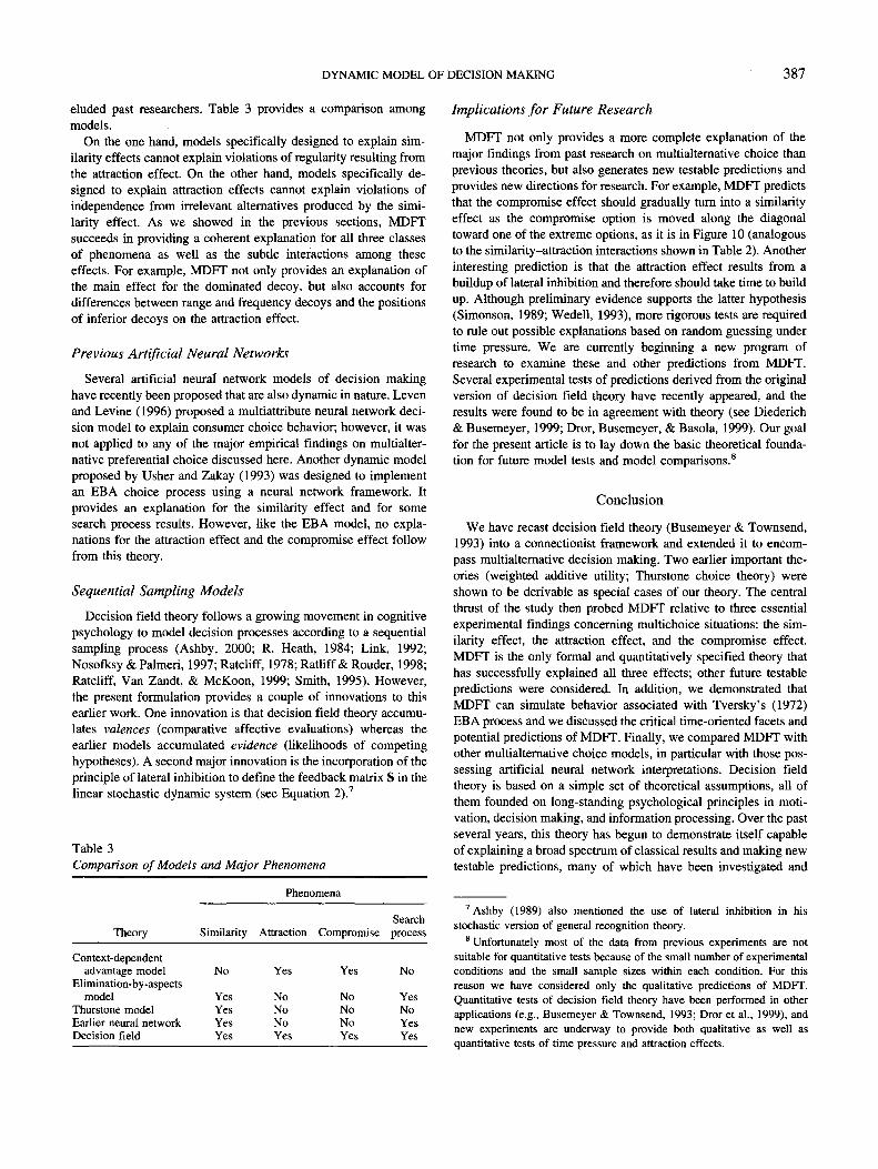
DYNAMIC MODEL OF DECISION MAKING 387
eluded past researchers. Table 3 provides a comparison amongmodels.
On the one hand, models specifically designed to explain sim-ilarity effects cannot explain violations of regularity resulting fromthe attraction effect. On the other hand, models specifically de-signed to explain attraction effects cannot explain violations ofindependence from irrelevant alternatives produced by the simi-larity effect. As we showed in the previous sections, MDFTsucceeds in providing a coherent explanation for all three classesof phenomena as well as the subtle interactions among theseeffects. For example, MDFT not only provides an explanation ofthe main effect for the dominated decoy, but also accounts fordifferences between range and frequency decoys and the positionsof inferior decoys on the attraction effect.
Previous Artificial Neural Networks
Several artificial neural network models of decision makinghave recently been proposed that are also dynamic in nature. Levenand Levine (1996) proposed a multiattribute neural network deci-sion model to explain consumer choice behavior; however, it wasnot applied to any of the major empirical findings on multialter-native preferential choice discussed here. Another dynamic modelproposed by Usher and Zakay (1993) was designed to implementan EBA choice process using a neural network framework. Itprovides an explanation for the similarity effect and for somesearch process results. However, like the EBA model, no expla-nations for the attraction effect and the compromise effect followfrom this theory.
Sequential Sampling Models
Decision field theory follows a growing movement in cognitivepsychology to model decision processes according to a sequentialsampling process (Ashby, 2000; R. Heath, 1984; Link, 1992;Nosofksy & Palmeri, 1997; Ratcliff, 1978; Ratliff & Rouder, 1998;Ratcliff, Van Zandt, & McKoon, 1999; Smith, 1995). However,the present formulation provides a couple of innovations to thisearlier work. One innovation is that decision field theory accumu-lates valences (comparative affective evaluations) whereas theearlier models accumulated evidence (likelihoods of competinghypotheses). A second major innovation is the incorporation of theprinciple of lateral inhibition to define the feedback matrix S in thelinear stochastic dynamic system (see Equation 2).7
Table 3Comparison of Models and Major Phenomena
Phenomena
TheorySearch
Similarity Attraction Compromise process
Context-dependentadvantage model
Elimination-by-aspectsmodel
Thurstone modelEarlier neural networkDecision field
No
YesYesYesYes
Yes
NoNoNoYes
Yes
NoNoNoYes
No
YesNoYesYes
Implications for Future Research
MDFT not only provides a more complete explanation of themajor findings from past research on multialternative choice thanprevious theories, but also generates new testable predictions andprovides new directions for research. For example, MDFT predictsthat the compromise effect should gradually turn into a similarityeffect as the compromise option is moved along the diagonaltoward one of the extreme options, as it is in Figure 10 (analogousto the similarity-attraction interactions shown in Table 2). Anotherinteresting prediction is that the attraction effect results from abuildup of lateral inhibition and therefore should take time to buildup. Although preliminary evidence supports the latter hypothesis(Simonson, 1989; Wedell, 1993), more rigorous tests are requiredto rule out possible explanations based on random guessing undertime pressure. We are currently beginning a new program ofresearch to examine these and other predictions from MDFT.Several experimental tests of predictions derived from the originalversion of decision field theory have recently appeared, and theresults were found to be in agreement with theory (see Diederich& Busemeyer, 1999; Dror, Busemeyer, & Basola, 1999). Our goalfor the present article is to lay down the basic theoretical founda-tion for future model tests and model comparisons.8
Conclusion
We have recast decision field theory (Busemeyer & Townsend,1993) into a connectionist framework and extended it to encom-pass multialternative decision making. Two earlier important the-ories (weighted additive utility; Thurstone choice theory) wereshown to be derivable as special cases of our theory. The centralthrust of the study then probed MDFT relative to three essentialexperimental findings concerning multichoice situations: the sim-ilarity effect, the attraction effect, and the compromise effect.MDFT is the only formal and quantitatively specified theory thathas successfully explained all three effects; other future testablepredictions were considered. In addition, we demonstrated thatMDFT can simulate behavior associated with Tversky's (1972)EBA process and we discussed the critical time-oriented facets andpotential predictions of MDFT. Finally, we compared MDFT withother multialternative choice models, in particular with those pos-sessing artificial neural network interpretations. Decision fieldtheory is based on a simple set of theoretical assumptions, all ofthem founded on long-standing psychological principles in moti-vation, decision making, and information processing. Over the pastseveral years, this theory has begun to demonstrate itself capableof explaining a broad spectrum of classical results and making newtestable predictions, many of which have been investigated and
7 Ashby (1989) also mentioned the use of lateral inhibition in hisstochastic version of general recognition theory.
8 Unfortunately most of the data from previous experiments are notsuitable for quantitative tests because of the small number of experimentalconditions and the small sample sizes within each condition. For thisreason we have considered only the qualitative predictions of MDFT.Quantitative tests of decision field theory have been performed in otherapplications (e.g., Busemeyer & Townsend, 1993; Dror et al., 1999), andnew experiments are underway to provide both qualitative as well asquantitative tests of time pressure and attraction effects.

388 ROE, BUSEMEYER, AND TOWNSEND
confirmed. The present work suggests that major multialternativechoice phenomena naturally ensue from the extended theory.
References
Ariely, D., & Wallsten, T. S. (1995). Seeking subjective dominance inmultidimensional space: An exploration of the asymmetric dominanceeffect. Organizational Behavior and Human Decision Processes, 63,223-232.
Aschenbrenner, K. M., Albert, D., & Schmalhofer, F. (1984). Stochasticchoice heuristics. Acta Psychologica, 56(1-3), 153-166.
Ashby, F. G. (1989). Stochastic general recognition theory. In D. Vickers& P. L. Smith (Eds.), Human information processing: Measures, mech-anisms and models (pp. 435-457). Amsterdam: Elsevier.
Ashby, F. G. (1992). Multidimensional models of perception and cognition.Hillsdale, NJ: Erlbaum.
Ashby, F. G. (2000). A stochastic version of general recognition theory.Journal of Mathematical Psychology, 44, 310-329.
Ashby, F. G., & Maddox, T. (1992). Complex decision rules in categori-zation: Contrasting novice and experienced performance. Journal ofExperimental Psychology: Human Perception and Performance, 18,50-71.
Ashby, F. G., & Townsend, J. T. (1986). Varieties of perceptual indepen-dence. Psychological Review, 93, 154-179.
Batsell, R. R., & Polking, J. C. (1985). A new class of market share models.Marketing Science, 4, 177-198.
Bettman, J. R., Johnson, E. J., & Payne, J. W. (1991). Consumer decisionmaking. In T. S. Robertson & H. H. Kassarjian (Eds.), Handbook ofconsumer behavior (pp. 50-84). Englewood Cliffs, NJ: Prentice Hall.
Bhattacharya, R. N., & Waymire, E. C. (1990). Stochastic processes withapplications. New York: Wiley.
Bock, R. D., & Jones, L. V. (1968). The measurement and prediction ofjudgment and choice. San Francisco: Holden-Day.
Bockenholt, U. (1992). Multivariate models of preference and choice. InF. G. Ashby (Ed.), Multidimensional Models of Perception and Cogni-tion, pp. 89-111. Hillsdale, NJ: Erlbaum.
Busemeyer, J. R., & Diederich, A. (2000). Survey of decision field theory.Manuscript submitted for publication.
Busemeyer, J. R., & Townsend, J. T. (1992). Fundamental derivations fromdecision field theory. Mathematical Social Sciences, 23, 255-282.
Busemeyer, J. R., & Townsend, J. T. (1993). Decision field theory: Adynamic cognition approach to decision making. Psychological Review,100, 432-459.
Candel, M. J. J. M. (1997). A probabilistic feature model for unfoldingtested for perfect and imperfect nestings. Journal of MathematicalPsychology, 41, 414-430.
Colonius, H. (1984). Stochastische theorien individuellen wahlverhastens[Stochastic theories of individual choice behavior]. Berlin, Germany:Springer-Verlag.
Cornsweet, T. (1970). Visual perception. Academic Press.Cox, D. R., & Miller, H. D. (1965). The theory of stochastic processes.
London: Chapman & Hall.De Soete, G., Feger, H., & Klauer, K. C. (Eds.). (1989). New developments
in probabilistic choice modeling. Amsterdam: North-Holland.Dhar, R., & Glazer, R. (1996). Similarity in context: Cognitive represen-
tations and violation of preference and perceptual invariance in con-sumer choice. Organizational Behavior and Human Decision Pro-cesses, 67, 280-293.
Diederich, A. (1997). Dynamic stochastic models for decision makingunder time constraints. Journal of Mathematical Psychology, 41, 260-274.
Diederich, A., & Busemeyer, J. R. (1999). Conflict and the stochasticdominance principle of decision making. Psychological Science, 10,353-359.
Dosher, B. A. (1984). Discriminating pre-experimental (semantic) fromlearned (episodic) associations: A speed accuracy study. Cognitive Psy-chology, 16, 519-555.
Dror, I. E., Busemeyer, J. R., & Basola, B. (1999). Decision making undertime pressure: An independent test of sequential sampling models.Memory & Cognition, 27, 713-725.
Edgell, S. E., & Geisler, W. S. (1980). A set-theoretic random utility modelof choice behavior. Journal of Mathematical Psychology, 21(3), 265-278.
Fischer, G. W., Jia, J., & Luce, M. F. (2000). Attribute conflict andpreference uncertainty: The RandMAU model. Management Sci-ence, 46, 669-684.
Gronlund, S. D., & Ratcliff, R. (1989). Time course of item and associativeinformation: Implications for global memory models. Journal of Exper-imental Psychology: Learning, Memory, and Cognition, 15, 846-858.
Grossberg, S. (1982). Studies of mind and brain: Neural principles oflearning, perception, development, cognition, and motor control. Hing-ham, MA: Reidel.
Grossberg, S. (1988). Neural networks and natural intelligence. Cam-bridge, MA: MIT Press.
Grossberg, S., & Gutowski, W. E. (1987). Neural dynamics of decisionmaking under risk: Affective balance and cognitive-emotional interac-tions. Psychological Review, 94, 300-318.
Heath, R. (1984). Random-walk and accumulator models of psychophys-ical discrimination: A critical evaluation. Perception, 13, 57—65.
Heath, T. B., & Chatterjee, S. (1991). How entrants affect multiple brands:A dual attraction mechanism. Advances in Consumer Research, 18,768-771.
Hintzman, D. L., & Curran, T. (1997). Comparing retrieval dynamics inrecognition memory and lexical decision. Journal of Experimental Psy-chology: General, 126, 228-247.
Huber, J., Payne, J. W., & Puto, C. (1982). Adding asymmetrically dom-inated alternatives: Violations of regularity and the similarity hypothe-sis. Journal of Consumer Research, 9, 90-98.
Huber, J., & Puto, C. (1983). Market boundaries and product choice:Illustrating attraction and substitution effects. Journal of ConsumerResearch, 10, 31-44.
Janis, I. L., & Mann, L. (1977). Decision making: A psychological analysisof conflict, choice, and commitment. New York: Free Press.
Keeney, R. L., & Raiffa, H. (1976). Decisions with multiple objectives:Preference and value tradeoffs. New York: Wiley.
Lehmann, D. R., & Pan, Y. (1994). Context effects, new brand entry, andconsideration sets. Journal of Marketing Research, 31, 364-374.
Leven, S. J., & Levine, D. S. (1996). Multiattribute decision making incontext: A dynamic neural network methodology. Cognitive Science, 20,271-299.
Levin, I. P., & Jasper, J. D. (1995). Phased narrowing: A new processtracing method for decision making. Organizational Behavior and Hu-man Decision Processes, 64, 1-8.
Link, S. W. (1992). The wave theory of difference and similarity. Hillsdale,NJ: Erlbaum.
Link, S. W., & Heath, R. (1975). A sequential theory of psychologicaldiscrimination. Psychometrika, 40, 77—111.
Luce, R. D. (1959). Individual choice behavior: A theoretical analysis.New York: Wiley.
MacKay, D. B., & Zinnes, J. L. (1995). Probabilistic multidimensionalunfolding: An anisotropic model for preference ratio judgments. Journalof Mathematical Psychology, 39, 99-111.
Marley, A. A. J. (1989). Random utility family that includes many of the"classical" models and has closed form choice probabilities and choicereaction times. British Journal of Mathematical and Statistical Psychol-ogy, 42, 13-36.
McClelland, J. L., & Rumelhart, D. E. (1981). An interactive activation

DYNAMIC MODEL OF DECISION MAKING 389
model of context effects in letter perception: I. An account of basicfindings. Psychological Review, 88, 375-407.
Mellers, B. A., & Biagini, K. (1994). Similarity and choice. PsychologicalReview, 101, 505-518.
Nosofsky, R. M., & Palmeri, T. J. (1997). Comparing exemplar-retrievaland decision-bound models of speeded perceptual classification. Per-ception & Psychophysics, 59, 1027-1048.
Payne, J. W., Bettman, J. R., & Johnson, E. J. (1993). The adaptivedecision maker. New York: Cambridge University Press.
Payne, J. W., Braunstein, M. L., & Carroll, J. S. (1978). Exploringpredecisional behavior: An alternative approach to decision research.Organizational Behavior and Human Decision Processes, 22, 17-44.
Ratcliff, R. (1978). A theory of memory retrieval. Psychological Re-view, 85, 59-108.
Ratcliff, R. (1980). A note on modeling accumulation of information whenthe rate of accumulation changes over time. Journal of MathematicalPsychology, 21, 178-184.
Ratcliff, R., & McKoon, G. (1982). Speed and accuracy in the processingof false statements about semantic information. Journal of ExperimentalPsychology: Learning, Memory, and Cognition, 8, 16-36.
Ratcliff, R., & McKoon, G. (1989). Similarity information versus relationalinformation: Differences in the time course of retrieval. Cognitive Psy-chology, 21, 139-155.
Ratcliff, R., & Rouder, J. N. (1998). Modeling response times for two-choice decisions. Psychological Science, 9, 347-356.
Ratcliff, R., Van Zandt, T., & McKoon, G. (1999). Connectionist anddiffusion models of reaction time. Psychological Review, 106, 261-300.
Ratneshwar, S., Shocker, A. D., & Stewart, D. W. (1987). Toward under-standing the attraction effect: The implications of product stimulusmeaningfulness and familiarity. Journal of Consumer Research, 13,520-527.
Reed, A. V. (1973). Speed-accuracy tradeoff in recognition memory.Science, 181, 574-576.
Rumelhart, D. E., & McClelland, J. L. (1986). Parallel distributed pro-cessing: Explorations in the microstructure of cognition: Vol. 1. Foun-dations. Cambridge, MA: MIT Press.
Russo, J. E., & Rosen, L. D. (1975). An eye fixation analysis of multialter-native choice. Memory & Cognition, 3, 267-276v
Samuelson, W., & Zeckhauser, R. (1988). Status quo bias in decisionmaking. Journal of Risk and Uncertainty, 1, 7-59.
Shepard, R. N. (1964). Attention and the metric structure of the stimulusspace. Journal of Mathematical Psychology, 1, 54-87.
Simon, H. A. (1955). A behavioral model of rational choice. QuarterlyJournal of Economics, 69, 99-118.
Simonson, I. (1989). Choice based on reasons: The case of attraction andcompromise effects. Journal of Consumer Research, 16, 158-174.
Simonson, I., & Tversky, A. (1992). Choice in context: Tradeoff contrastand extremeness aversion. Journal of Marketing Research, 24, 281-295.
Sjoberg, L. (1977). Choice frequency and similarity. Scandinavian Journalof Psychology, 18, 103-115.
Smith, P. L. (1995). Psychophysically principled models of visual simplereaction time. Psychological Review, 102, 567—593.
Smith, P. L. (2000). Stochastic dynamic models of response time andaccuracy: A foundational primer. Journal of Mathematical Psychol-ogy, 44, 408-463.
Takane, Y. (1989). Analysis of covariance structures and probabilisticbinary choice data. In G. De Soete, H. Feger, & K. C. Klauer (Eds.), Newdevelopments in probabilistic choice modeling (pp. 139-160). Amster-dam: North-Holland.
Thurstone, L. L. (1959). The measurement of values. Chicago: Universityof Chicago Press.
Townsend, J. T., & Busemeyer, J. R. (1995). Dynamic representation ofdecision-making. In R. F. Port & T. van Gelder (Eds.), Mind as motion(pp. 101-120). Cambridge, MA: MIT Press.
Tversky, A. (1969). Intransitivity of preferences. Psychological Re-view, 76, 31-48.
Tversky, A. (1972). Elimination by aspects: A theory of choice. Psycho-logical Review, 79, 281-299.
Tversky, A., & Simonson, I. (1993). Context dependent preferences. Man-agement Science, 39, 1179-1189.
Usher, M., & Zakay, D. (1993). A neural network model for attribute-baseddecision processes. Cognitive Science, 17, 349-396.
Vickers, D. (1979). Decision processes in visual perception. New York:Academic Press.
Vickers, D. B. J., Smith, P., & Brown, M. (1985). Experimental paradigmsemphasizing state or process limitations: I. Effects of speed-accuracytradeoffs. Acta Psychologica, 59, 129-161.
Von Winterfeldt, D., & Edwards, W. (1986). Decision analysis and be-havioral research. Cambridge, England: Cambridge University Press.
Wedell, D. H. (1991). Distinguishing among models of contextually in-duced preference reversals. Journal of Experimental Psychology, 17,767-778.
Wedell, D. H. (1993, November). Studying effects of different decoys onchoice in a within-subject design. Paper presented at the 34th AnnualMeeting of the Psychonomic Society, St. Louis, MO.
Wickelgren, W., Corbett, A., & Dosher, B. (1980). Priming and retrievalfrom short-term memory: A speed accuracy trade-off analysis. Journalof Verbal Learning and Verbal Behavior, 19, 387-404.
Wright, P., & Barbour, F. (1977). Phased decision strategies: Sequels to aninitial screening. In M. Starr & M. Zeleny (Eds.), Multiple criteriadecision making: TIMS studies in the management sciences, (Chap. 6,pp. 1—10). Amsterdam: North-Holland.
(Appendixes follow)

390 ROE, BUSEMEYER, AND TOWNSEND
Appendix A
Derivations for Content-Dependent Advantage Model
This appendix proves that the context-dependent advantage model de-veloped by Tversky and Simonson (1993) cannot simultaneously explainthe similarity effect and the compromise effect. Tversky and Simonsonnever attempted to apply the model to the similarity effect, although itclearly can be applied in the same manner as the compromise effect.
Their model requires the definition of four parameters: a = the uniqueadvantage of option A over B; ft = the unique advantage of option B overA; y = unique advantage of option A over S; and A = the uniqueadvantage of option S over A. Tversky and Simonson (1993) based all theirderivations on the case where a = /3, so that according to their model, theoptions A and B are chosen equally often in the binary case.
Following Tversky and Simonson's (1993) derivation for the compro-mise effect, the similar option S, as shown in Figure 1, has a uniqueadvantage, A, over A, which is equal to the unique advantage, 7, of A overS, so that 7 = A = e. The main difference between the compromise andsimilarity effect is that for the latter, e is an arbitrarily small magnitude.Applying their formulas to the similarity case yields
[ )3 0 + 7 1
P + 8(a) + J3 + 7 + 8(a + A)J7 + 8(
a + e8(a) a
In the above formulas, 6 is an unknown context weight parameter, andS(x) > x is assumed to be a convex function. Strict convexity was requiredby Tversky and Simonson (1993, p. 1187) to explain the compromiseeffect.
To explain the similarity effect, it is necessary to have V(B) > V(A). Butthis is impossible if 5(x) is strictly convex. To see this, note that if S(x) isstrictly convex, then for any a > 0, S(a) > aS'(O), where S'(0) is thederivative of 8 evaluated at zero. This implies that as e —> 0, 5(a + e)/(a +€) > S(e)/€. But the last inequality implies that
a + e
a + e + S(a + e) e+ 8(e) '(Al)
and finally, this inequality (Equation Al) implies V(A) > V(B), contrary tothe similarity effect. For example, consider the commonly used case whered(x) = xs is a power function and define 17 = 1 + (e/a).
£ ) > € ' > e5(« + e)8
> V(A)> V(B).
For the linear case, it is easy to show that S(x) = Sx —> V(A) = V(B), againcontrary to the desired empirical finding for the similarity effect, V(B) >V(A). In fact, the inequality (Equation Al) is exactly the same inequalitythat must be satisfied to produce the compromise effect (see Tversky andSimonson, 1993, p. 1187), hence their need for imposing the convexityproperty. But this same property rules out the possibility of explaining thesimilarity effect.
Appendix B
Derivations for Decision Field Theory
This appendix derives the mathematical formula used to compute theprobabilities for Equation 3. The valence vector defined by Equation 1 isa linear transformation of the stochastic weight vector, W(r). This weightvector is assumed to change across time according to a stationary stochasticprocess. The stationarity assumption for the weights implies that thevalence vector (V) is also a stationary stochastic process with mean E[\(f>]= E[CM,W,(f) + e(r)] = CM,£[W,(f)] + E[e(t)] = CM,w, + 0 = fiand variance-covariance matrix at each time point given by Cov[\(t)] =Cov[CMjW,(0 + e(01 = CMjCovtW^JM'.C' + Cov[e(t)] =CM,¥MiC' + y = <fr, where * = Cov[Wi(f)] = CKW^r) - Wi)(W,(f)— w,)'] is the variance-covariance matrix for the primary weights, and y= Cov[e(f)l = E[e(t)e(t)'] is the variance-covariance matrix of the resid-uals. Analogous to a factor analytic model (cf. Takane, 1989), the residualsare assumed to be uncorrelated with the primary dimensions and uncorre-lated with each other. This implies that y is a diagonal matrix.
The effects of the feedback matrix on the evolution of preference overtime can be seen more clearly by expanding Equation 2:
P(r) = 2,=0.,-iS''V(* -j) + S'P(O). (Bl)
This equation shows that the current preference state can be viewed as aweighted sum of the previous input valences. The weight placed on each
previous input is determined by the feedback matrix raised to a power,where the power equals the lag between the current state and the previousinput. For this system to be stable, the eigenvalues of the feedback matrixmust be less than one in magnitude. In this case, the effect of the feedbackmatrix decays toward zero as the lag increases in value. Taking expecta-tions and simplifying produces the mean preference over time:
= £[P(r)] = (I - S)-'(I S-P(0). (B2)
For stable systems, as t —» °°, then g(r) —» (I — S) Vi which is a simpleformula for analyzing the effects of the feedback matrix on the asymptoticmean preference state. If weights are identically and independently distrib-uted over time (see Footnote 1), then the variance—covariance matrix of thepreference state evolves over time according to fl(t) = cov[P(0] =E{(P(t) - E(P(t)])(f(t) - £[P«])') = 2,=0.,-iS'*S''.
On the basis of the multivariate central limit theorem, the distribution ofthe preference states P(f) converges to the multivariate normal distributionas the number of steps (t) in Equation B1 becomes large. If the time periodbetween steps is small, then this convergence will occur very rapidly.Given that P(r) is distributed according to the multivariate normal distri-bution with mean g(i) and variance-covariance matrix ft(r), then theprobability of choosing A from the set {A, B, C} at fixed time point t is:
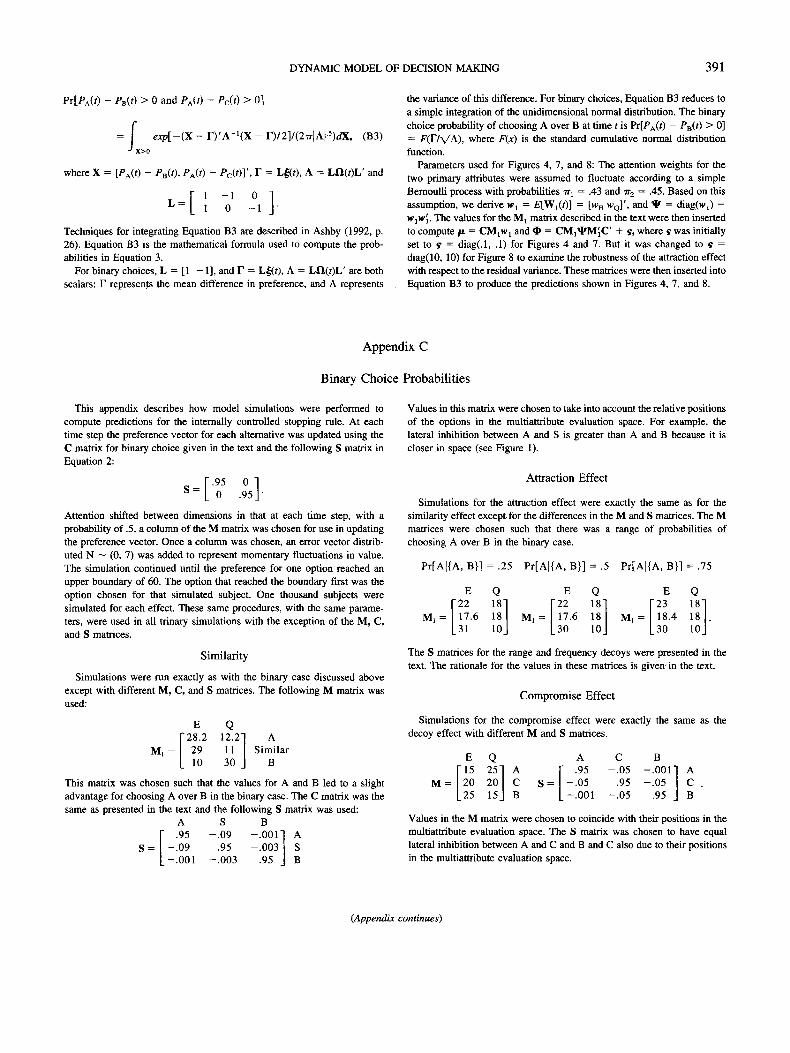
DYNAMIC MODEL OF DECISION MAKING 391
Pr[PA« - P,(t) > 0 and />A(r) - Pc(i) > 0]
exp[-(K - D'A-'(X - r)/2]/(27r|A|-5)<*X, (B3)>
where X = [PA(t) - PB(t), PA(t) - Pc(t)Y, T = L&t), A = L«(r)L' and
L = L 1 0 -1 J '
Techniques for integrating Equation B3 are described in Ashby (1992, p.26). Equation B3 is the mathematical formula used to compute the prob-abilities in Equation 3.
For binary choices, L = [1 -1], and T = L£(r), A = Lfl(r)L' are bothscalars: F represents the mean difference in preference, and A represents
the variance of this difference. For binary choices, Equation B3 reduces toa simple integration of the unidimensional normal distribution. The binarychoice probability of choosing A over B at time t is Pr[/'A(r) - PB(t) > 0]= F(I7\/A), where F(x) is the standard cumulative normal distributionfunction.
Parameters used for Figures 4, 7, and 8: The attention weights for thetwo primary attributes were assumed to fluctuate according to a simpleBernoulli process with probabilities irl = .43 and ir2 = .45. Based on thisassumption, we derive 1?! = £[Wt(f)] = [WE WQ]', and 9 = diag^,) -w^w',. The values for the Mj matrix described in the text were then insertedto compute ft = CM^, and <I» = CM^MJC' + s, where s was initiallyset to 9 = diag(.l, .1) for Figures 4 and 7. But it was changed to s =diag(10, 10) for Figure 8 to examine the robustness of the attraction effectwith respect to the residual variance. These matrices were then inserted intoEquation B3 to produce the predictions shown in Figures 4, 7, and 8.
Appendix C
Binary Choice Probabilities
This appendix describes how model simulations were performed tocompute predictions for the internally controlled stopping rule. At eachtime step the preference vector for each alternative was updated using theC matrix for binary choice given in the text and the following S matrix inEquation 2:
S =.95 00 .95
Attention shifted between dimensions in that at each time step, with aprobability of .5, a column of the M matrix was chosen for use in updatingthe preference vector. Once a column was chosen, an error vector distrib-uted N ~ (0, 7) was added to represent momentary fluctuations in value.The simulation continued until the preference for one option reached anupper boundary of 60. The option that reached the boundary first was theoption chosen for that simulated subject. One thousand subjects weresimulated for each effect. These same procedures, with the same parame-ters, were used in all trinary simulations with the exception of the M, C,and S matrices.
Similarity
Simulations were run exactly as with the binary case discussed aboveexcept with different M, C, and S matrices. The following M matrix wasused:
M,
E28.22910
Q12.21130
ASimilar
B
This matrix was chosen such that the values for A and B led to a slightadvantage for choosing A over B in the binary case. The C matrix was thesame as presented in the text and the following S matrix was used:
A S B.95 -.09 -.001] A
S = -.09 .95 -.003 S.OOI -.003 .95 J B
Values in this matrix were chosen to take into account the relative positionsof the options in the multiattribute evaluation space. For example, thelateral inhibition between A and S is greater than A and B because it iscloser in space (see Figure 1).
Attraction Effect
Simulations for the attraction effect were exactly the same as for thesimilarity effect except for the differences in the M and S matrices. The Mmatrices were chosen such that there was a range of probabilities ofchoosing A over B in the binary case.
Pr[A|{A, B}] = .25 Pr[A|{A, B}] = .5 Pr[A|{A, B}] = .75
M,
E Q
'22 1817.6 1831 10
M
E'22
= | 17.630
M,
E Q23 18
= | 18.4 1830 10
The S matrices for the range and frequency decoys were presented in thetext. The rationale for the values in these matrices is given in the text.
Compromise Effect
Simulations for the compromise effect were exactly the same as thedecoy effect with different M and S matrices.
E Q
'15 25] A20 20 C25 15 B
A C B.95 -.05 -.001
S= | -.05 .95 -.05-.001 -.05 .95
ACB
Values in the M matrix were chosen to coincide with their positions in themultiattribute evaluation space. The S matrix was chosen to have equallateral inhibition between A and C and B and C also due to their positionsin the multiattribute evaluation space.
(Appendix continues)

392 ROE, BUSEMEYER, AND TOWNSEND
Search Variability
Values for the M matrix were chosen such that each option had 12attributes, 4 of which had a high value, 4 medium, and 4 low (1,0, -1,respectively). Attribute values were ordered such that no option dominatedanother. Simulations were run separately for one of three choice setsizes: 2, 7, or 12. Hence, for the 12-option set, the original M matrix wasa 12 (number of options) X 12 (number of attributes) matrix with each rowrepresenting values across dimensions for each alternative. For the 7- and2-option sets the M matrix was constructed similarly and were of size7 X 12 and 2 X 12, respectively.
Because some options are eliminated from the choice set during delib-eration, the size of all of the matrices changed. The S matrix consisted ofa number of options remaining X number of options remaining diagonalmatrix with .95 on the diagonal and zeros everywhere else. The C matrix
was constructed to compare each alternative with the average of all otheralternatives.
The upper preference boundary to choose an option was set at 50. Thelower boundary to discard an option was set at -30, -20, -10 for the 2-,7-, and 12-option sets, respectively. Attention shifted from one dimensionto another in that on each trial there was a 95% probability that the samedimension would be used at the next time step and a 5% probability ofmoving to the next dimension. An error component of N ~ (0, 7) wasadded to the column of the M matrix chosen on each trial. Simulationswere run for each subject until an option crossed the upper boundary, allbut one option was discarded, or all 12 dimensions were cycled through.
Received July 2, 1999Revision received July 19, 2000
Accepted July 22, 2000 •
AMERICAN PSYCHOLOGICAL ASSOCIATIONSUBSCRIPTION CLAIMS INFORMATION Today's Date:.
We provide this form to assist members, institutions, and nonmember individuals with any subscription problems. With theappropriate information we can begin a resolution. If you use the services of an agent, please do NOT duplicate claims throughthem and directly to us. PLEASE PRINT CLEARLY AND IN INK IF POSSIBLE.
PRINT FULL NAME OR KEY NAME OF rNSnTUTlON MEMBER OR CUSTOMERNUMBER (MAYBE FOUND ON ANYPAST ISSUE LABEL)
DATE YOUR ORDER WAS MAILED (OR PHONED)
__PREPATD CHECK __CHARGECHECK/CARD CLEARED DATE:_
CITY STATE/COUNTRY
YOUR NAME AND PHONE NUMBER
TITLE
(If possible, send a copy, front and back, of your cancelled check to help us in our researchof your claim.)
ISSUES: MISSING ___ DAMAGED
VOLUME OR YEAR NUMBER OR MONTH
Thank you. Once a claim is received and resolved, delivery of replacement issues routinely takes 4-6 weeks.
——^—^———. (TO BE FILLED OUT BY APA STAFF) ——————
DATE RECEIVED:.ACTION TAKEN: _STAFF NAME:
DATE OF ACTION: _INV.NO.&DATE:LABEL NO. & DATE:
Send this form to APA Subscription Claims, 750 First Street, NE, Washington, DC 20002-4242
PLEASE DO NOT REMOVE. A PHOTOCOPY MAY BE USED.