Detecting Salient Contours Using

Orientation Energy Distribution

CPSC 636 Slide12, Spring 2012

Yoonsuck Choe

Co-work with S. Sarma and H.-C. Lee

Based on Lee and Choe (2003); Sarma (2003); Sarma and Choe (2006)

1

The Problem: How Does the Visual System Detect

Salient Contours?

• Neurons in the visual cortex have Gabor-like receptive fields.

• Looking at the response properties of these neurons can help

us answer the question.

• The simplest statistical property can be measured by looking at

the response histogram.

Questioning from a slightly different perspective, “how can the

particular response property of visual cortical neurons be utilized

by later processing?”

2

Part I: Thresholding Based on

Response Distribution

3

Observation

• Grayscale intensity distributions are quite different across

different images.

• However, Gabor response distributions are quite similar across

different images.

4

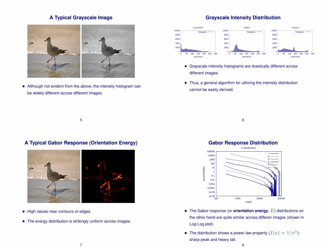
A Typical Grayscale Image

• Although not evident from the above, the intensity histogram can

be widely different across different images.

5

Grayscale Intensity Distribution

0

2000

4000

6000

8000

10000

0 50 100 150 200 250 300

gray-level

yosemite07

histogram

0

2000

4000

6000

8000

10000

0 50 100 150 200 250 300

gray-level

bird08

histogram

0

2000

4000

6000

8000

10000

0 50 100 150 200 250 300

gray-level

rocky10

histogram

• Grayscale intensity histograms are drastically different across

different images.

• Thus, a general algorithm for utilizing the intensity distribution

cannot be easily derived.

6

A Typical Gabor Response (Orientation Energy)

• High values near contours or edges.

• The energy distribution is strikingly uniform across images.

7

Gabor Response Distribution

1e-06

1e-05

0.0001

0.001

0.01

0.1

1

10

100

1000

10000

100000

100 1000 10000 100000

log

prob

abili

tylog(E)

E distributions

fedcba

• The Gabor response (or orientation energy;E) distributions on

the other hand are quite similar across differen images (shown in

Log-Log plot).

• The distribution shows a power law property (f(x) = 1/xa):

sharp peak and heavy tail.8

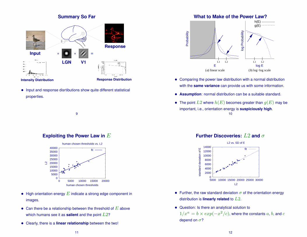
Summary So Far

* * =

LGN V1

Input

Intensity Distribution Response Distribution

Response

• Input and response disrtibutions show quite different statistical

properties.

9

What to Make of the Power Law?

L2L1 L2L1

g(E)h(E)

a( ) linear scale b( ) log−log scale

log

Pro

babi

lity

Pro

babi

lity

E log E

• Comparing the power law distribution with a normal distribution

with the same variance can provide us with some information.

• Assumption: normal distribution can be a suitable standard.

• The point L2 where h(E) becomes greater than g(E) may be

important, i.e., orientation energy is suspiciously high.10

Exploiting the Power Law in E

05000

10000150002000025000300003500040000

0 5000 10000 15000 20000

L2

human chosen thresholds

human chosen thresholds vs. L2

fit

• High orientation energyE indicate a strong edge component in

images.

• Can there be a relationship between the threshold ofE above

which humans see it as salient and the point L2?

• Clearly, there is a linear relationship between the two!

11

Further Discoveries: L2 and σ

0

2000

4000

6000

8000

10000

12000

14000

5000 10000 15000 20000 25000 30000

stan

dard

dev

iatio

n of

E

L2

L2 vs. SD of E

fit

• Further, the raw standard deviation σ of the orientation energy

distribution is linearly related to L2.

• Question: Is there an analytical solution to

1/xa = b× exp(−x2/c), where the constants a, b, and c

depend on σ?

12

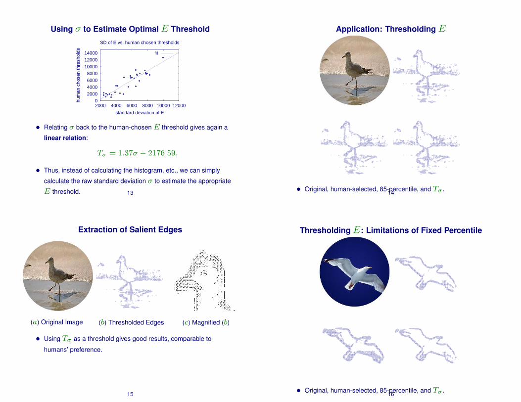
Using σ to Estimate Optimal E Threshold

02000400060008000

100001200014000

2000 4000 6000 8000 10000 12000

hum

an c

hose

n th

resh

olds

standard deviation of E

SD of E vs. human chosen thresholds

fit

• Relating σ back to the human-chosenE threshold gives again a

linear relation:

Tσ = 1.37σ − 2176.59.

• Thus, instead of calculating the histogram, etc., we can simply

calculate the raw standard deviation σ to estimate the appropriate

E threshold. 13

Application: Thresholding E

• Original, human-selected, 85-percentile, and Tσ .14

Extraction of Salient Edges

(a) Original Image (b) Thresholded Edges (c) Magnified (b)

• Using Tσ as a threshold gives good results, comparable to

humans’ preference.

15

Thresholding E: Limitations of Fixed Percentile

• Original, human-selected, 85-percentile, and Tσ .16

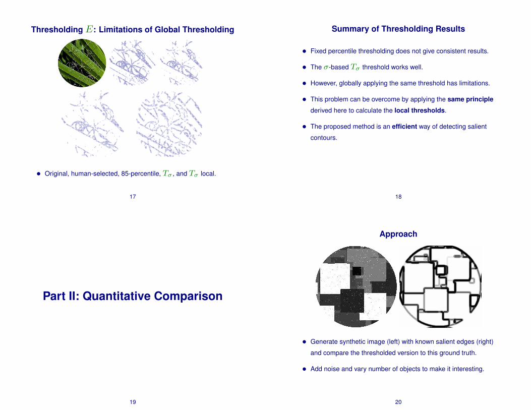
Thresholding E: Limitations of Global Thresholding

• Original, human-selected, 85-percentile, Tσ , and Tσ local.

17

Summary of Thresholding Results

• Fixed percentile thresholding does not give consistent results.

• The σ-based Tσ threshold works well.

• However, globally applying the same threshold has limitations.

• This problem can be overcome by applying the same principle

derived here to calculate the local thresholds.

• The proposed method is an efficient way of detecting salient

contours.

18

Part II: Quantitative Comparison

19

Approach

• Generate synthetic image (left) with known salient edges (right)

and compare the thresholded version to this ground truth.

• Add noise and vary number of objects to make it interesting.

20

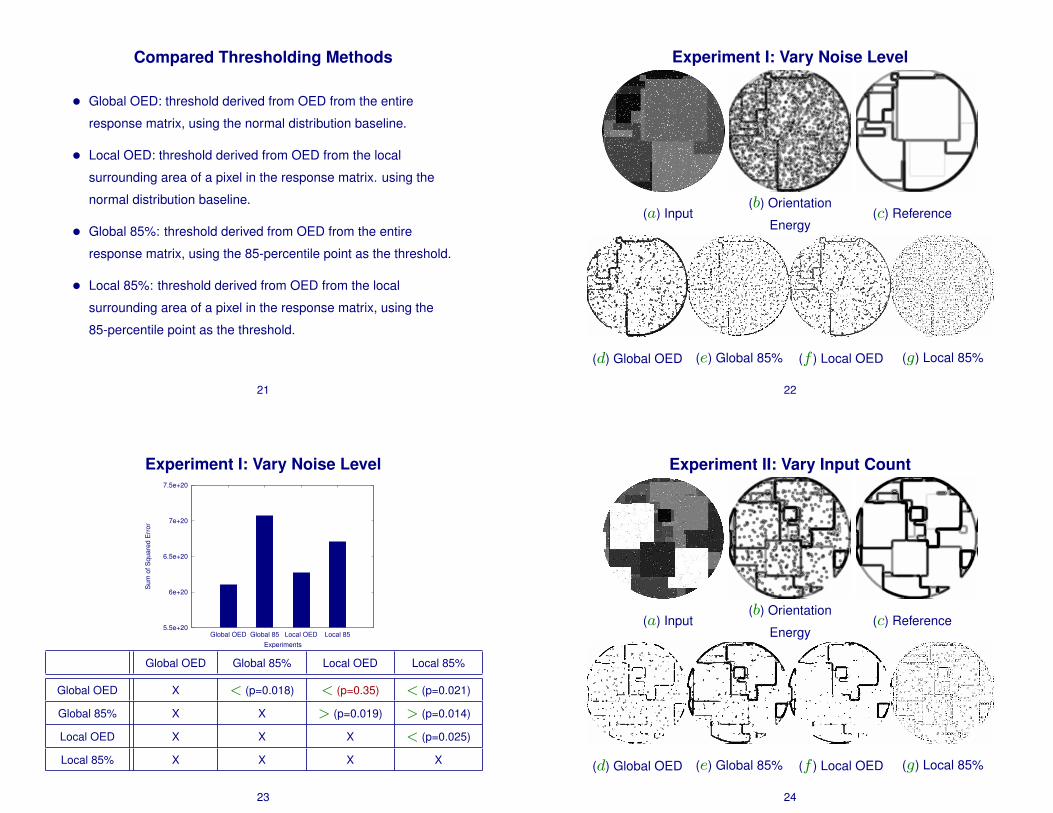
Compared Thresholding Methods

• Global OED: threshold derived from OED from the entire

response matrix, using the normal distribution baseline.

• Local OED: threshold derived from OED from the local

surrounding area of a pixel in the response matrix. using the

normal distribution baseline.

• Global 85%: threshold derived from OED from the entire

response matrix, using the 85-percentile point as the threshold.

• Local 85%: threshold derived from OED from the local

surrounding area of a pixel in the response matrix, using the

85-percentile point as the threshold.

21

Experiment I: Vary Noise Level

(a) Input(b) Orientation

Energy(c) Reference

(d) Global OED (e) Global 85% (f ) Local OED (g) Local 85%

22

Experiment I: Vary Noise Level

5.5e+20

6e+20

6.5e+20

7e+20

7.5e+20

Local 85Local OEDGlobal 85Global OED

Sum

of S

quar

ed E

rror

Experiments

Global OED Global 85% Local OED Local 85%

Global OED X < (p=0.018) < (p=0.35) < (p=0.021)

Global 85% X X > (p=0.019) > (p=0.014)

Local OED X X X < (p=0.025)

Local 85% X X X X

23

Experiment II: Vary Input Count

(a) Input(b) Orientation

Energy(c) Reference

(d) Global OED (e) Global 85% (f ) Local OED (g) Local 85%

24

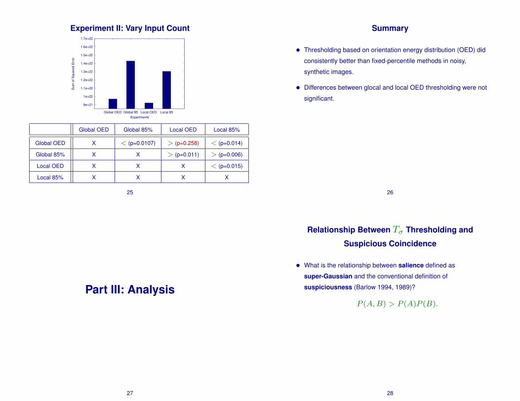
Experiment II: Vary Input Count

9e+21

1e+22

1.1e+22

1.2e+22

1.3e+22

1.4e+22

1.5e+22

1.6e+22

1.7e+22

Local 85Local OEDGlobal 85Global OED

Sum

of S

quar

ed E

rror

Experiments

Global OED Global 85% Local OED Local 85%

Global OED X < (p=0.0107) > (p=0.258) < (p=0.014)

Global 85% X X > (p=0.011) > (p=0.006)

Local OED X X X < (p=0.015)

Local 85% X X X X

• Error in Thresholding (Both Experiments): The

global and local OED-derived method have

significantly smaller sum of squared error values

than the fixed 85-percentile methods.

25

Summary

• Thresholding based on orientation energy distribution (OED) did

consistently better than fixed-percentile methods in noisy,

synthetic images.

• Differences between glocal and local OED thresholding were not

significant.

26

Part III: Analysis

27

Relationship Between Tσ Thresholding and

Suspicious Coincidence

• What is the relationship between salience defined as

super-Gaussian and the conventional definition of

suspiciousness (Barlow 1994, 1989)?

P (A,B) > P (A)P (B).

28

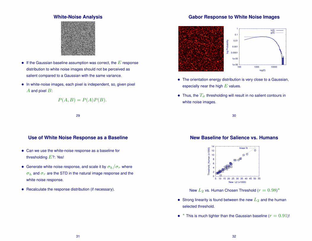
White-Noise Analysis

• If the Gaussian baseline assumption was correct, theE response

distribution to white noise images should not be perceived as

salient compared to a Gaussian with the same variance.

• In white-noise images, each pixel is independent, so, given pixel

A and pixelB:

P (A,B) = P (A)P (B).

29

Gabor Response to White Noise Images

1e-06

1e-05

0.0001

0.001

0.01

0.1

1

100 1000 10000

log

Pro

babi

lity

log(E)

h(E)g(E)

• The orientation energy distribution is very close to a Gaussian,

especially near the highE values.

• Thus, the Tσ thresholding will result in no salient contours in

white noise images.

30

Use of White Noise Response as a Baseline

• Can we use the white-noise response as a baseline for

thresholdingE?: Yes!

• Generate white noise response, and scale it by σh/σr where

σh and σr are the STD in the natural image response and the

white noise response.

• Recalculate the response distribution (if necessary).

31

New Baseline for Salience vs. Humans

0

2

4

6

8

10

12

14

5 10 15 20 25 30 35 40 45 50 55

Thre

shol

d_H

uman

(x10

00)

New_L2 (x1000)

linear fit

New L2 vs. Human Chosen Threshold (r = 0.98)∗

• Strong linearity is found between the new L2 and the human

selected threshold.

• ∗ This is much tighter than the Gaussian baseline (r = 0.91)!

32

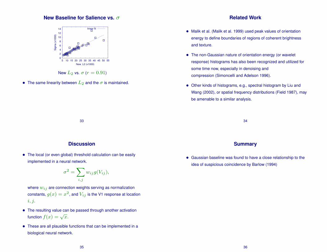
New Baseline for Salience vs. σ

0

2

4

6

8

10

12

14

5 10 15 20 25 30 35 40 45 50 55

Sig

ma

(x10

00)

New_L2 (x1000)

linear fit

New L2 vs. σ (r = 0.91)

• The same linearity between L2 and the σ is maintained.

33

Related Work

• Malik et al. (Malik et al. 1999) used peak values of orientation

energy to define boundaries of regions of coherent brightness

and texture.

• The non-Gaussian nature of orientation energy (or wavelet

response) histograms has also been recognized and utilized for

some time now, especially in denoising and

compression (Simoncelli and Adelson 1996).

• Other kinds of histograms, e.g., spectral histogram by Liu and

Wang (2002), or spatial frequency distributions (Field 1987), may

be amenable to a similar analysis.

34

Discussion

• The local (or even global) threshold calculation can be easily

implemented in a neural network.

σ2 =∑i,j

wijg(Vij),

wherewij are connection weights serving as normalization

constants, g(x) = x2, and Vij is the V1 response at location

i, j.

• The resulting value can be passed through another activation

function f(x) =√x.

• These are all plausible functions that can be implemented in a

biological neural network.

35

Summary

• Gaussian baseline was found to have a close relationship to the

idea of suspicious coincidence by Barlow (1994)

36

Lesson Learned

• Studying statistical properties of raw natural signal distributions

can be useful in determining why the visual system is structured

in the current form (e.g., PCA, ICA, etc. predicts the receptive

field shape).

• However, what’s more interesting is that the response

properties of cortical neurons can have certain invariant

properties and this can be exploited.

• So, we need to go beyond finding out what receptive fields look

like and why, and start to explore how cortical neuron response

can be utilized by the rest of the brain.

37

Conclusion

• Cortical response distribution has a unique invariant property (the

power-law).

• Such properties can be exploited in tasks such as salient contour

detection.

• Gaussian distribution forms a good baseline for determining the

threshold.

• The above may be related to the idea of suspicious coincidence.

38

ReferencesBarlow, H. (1994). What is the computational goal of the neocortex? In Koch, C., and Davis, J. L., editors, Large Scale

Neuronal Theories of the Brain, 1–22. Cambridge, MA: MIT Press.

Barlow, H. B. (1989). Unsupervised learning. Neural Computation, 1:295–311.

Field, D. J. (1987). Relations between the statistics of natural images and the response properties of cortical cells. Journalof the Optical Society of America A, 4:2379–2394.

Lee, H.-C., and Choe, Y. (2003). Detecting salient contours using orientation energy distribution. In Proceedings of theInternational Joint Conference on Neural Networks, 206–211. IEEE.

Liu, X., and Wang, D. (2002). A spectral histogram model for texton modeling and texture discrimination. Vision Research,42:2617–2634.

Malik, J., Belongie, S., Shi, J., and Leung, T. K. (1999). Textons, contours and regions: Cue integration in image segmen-tation. In ICCV(2), 918–925.

Sarma, S., and Choe, Y. (2006). Salience in orientation-filter response measured as suspicious coincidence in naturalimages. In Gil, Y., and Mooney, R., editors, Proceedings of the 21st National Conference on Artificial Intelli-gence(AAAI 2006), 193–198.

38-1

Sarma, S. P. (2003). Relationship between suspicious coincidence in natural images and contour-salience in orientedfilter responses. Master’s thesis, Department of Computer Science, Texas A&M University.

Simoncelli, E. P., and Adelson, E. H. (1996). Noise removal via bayesian wavelet coring. In Proceedings of IEEEInternational Conference on Image Processing, vol. I, 379–382.

38-2