multi-view canonical correlation analysis
TRANSCRIPT

MULTI-VIEW CANONICAL CORRELATION
ANALYSIS
Jan Rupnik

Doctoral DissertationJoºef Stefan International Postgraduate SchoolLjubljana, Slovenia
Supervisor: Prof. Dr. Dunja Mladeni¢, Joºef Stefan Institute and Joºef Stefan Interna-tional Postgraduate School, Jamova 39, Ljubljana, SloveniaCo-Supervisor: Prof. Dr. John Shawe-Taylor, Department of Computer Science, Univer-sity College London, Gower Street London WC1E 6BT, United Kingdom
Evaluation Board:Prof. Dr. Nada Lavra£, Chair, Joºef Stefan Institute and Joºef Stefan International Post-graduate School, Jamova 39, Ljubljana, SloveniaProf. Dr. Bor Plestenjak, Member, Faculty of Mathematics and Physics, University ofLjubljana, Jadranska 21, Ljubljana, SloveniaProf. Dr. Nicolò Cesa-Bianchi, Member, Department of Computer Science, University ofMilan, via Comelico 39 20135 Milano, Italy
Jan Rupnik
MULTI-VIEW CANONICAL CORRELATION ANALYSIS
Doctoral Dissertation
KANONI�NAKORELACIJSKA ANALIZA ZA VE�MNO�ICSPREMENLJIVK
Doktorska disertacija
Supervisor: Prof. Dr. Dunja Mladeni¢
Co-Supervisor: Prof. Dr. John Shawe-Taylor
Ljubljana, Slovenia, January 2016


To Zala


vii
Acknowledgments
I would like to express great appreciation to my PhD supervisor Prof. Dunja Mladeni¢and co-supervisor Prof. John Shawe-Taylor for their guidance and advice throughout mystudies. Special thanks go to Primoº �kraba for his invaluable advice and contributionsto my work. I would also like to thank Marko Grobelnik for providing inspiration andencouragement for my research work.
Assistance provided by my collaborators Andrej Muhi£, Blaº Fortuna, Gregor Lebanand Sabrina Guettes was greatly appreciated. It was my great pleasure working with you.I would also like to thank my friends from UCL: Tom Diethe, David Roi Hardoon andZakria Hussain for great company and discussions during my visits to UCL.
My gratitude goes to the members of my doctoral committee, Prof. Nada Lavra£, Prof.Bor Plestenjak and Prof. Nicolò Cesa-Bianchi, for their valuable comments and remarks.
Finally, I wish to thank Zala, my parents Darja and Erik and my sister Nika for theirsupport and encouragement.
The author gratefully acknowledges funding by the projects SMART (IST-5-033917-STP), X-LIKE (ICT-257790-STREP), MultilingualWeb (PSP-2009.5.2 Agr.# 250500),TransLectures (FP7-ICT-2011-7), PlanetData (ICT-257641-NoE), RENDER (ICT-257790-STREP), XLime (FP7-ICT-611346), and META-NET (ICT-249119-NoE).


ix
Abstract
Matrix factorization represents a popular approach in pattern analysis and is used totackle many problems, such as: collaborative �ltering, imputing missing data, denoisingdata, dimensionality reduction, data visualization and exploratory analysis.
This thesis is focused on factorization based pattern analysis methods for multiviewlearning problems: that is problems where each data instance is represented by multipleviews of an underlying object, encoded by multiple feature sets. As an example of amultiview problem consider a dataset where each instance has two representations: avisual image and a textual description. The patterns of interest are pairs of functions overimages and texts that are strongly related over the observed data.
Canonical Correlation Analysis (CCA) is designed to extract patterns from data setswith two views. This thesis focuses on two generalizations of CCA, which were proposed inthe literature: Sum of Correlations (SUMCOR) and Sum of Squared Correlations SSCOR.The SUMCOR problem formulation is interesting from the optimization perspective by itsown right, since it emerges in other problems as well.
We study several aspects of the generalizations. We �rst present a provably convergentnovel algorithm for �nding non-linear higher order patterns, which is based on an iterativeapproach for solving multivariate eigenvalue problems. We show that SUMCOR in generalis NP-hard and then study its reformulation to a computationally tractable Semide�niteProgramming (SDP) problem. Based on the reformulation we derive several computation-ally feasible bounds on global optimality, which complement the locally optimal solutions.We introduce a new preprocessing step for dealing with large scale SDP problems thatarise from an application to cross-lingual text analysis. We investigated how to apply ourmethods to real datasets with missing data. The particular structure of missing data in theproblem considered leads to a simpli�cation of the SSCOR optimization problem, which isreduced to a tractable eigenvalue problem. We show how the algorithms apply to buildingcross-lingual similarity models and apply the models on the task of cross-lingual clusterlinking. The approach to cross-lingual cluster linking is used in a real-time global analysisof news streams in multiple languages.


xi
Povzetek
Metode, ki temeljijo na matri£ni faktorizaciji, predstavljajo pomemben pristop k analizivzorcev in podatkovnemu rudarjenju. Naloge, ki jih lahko prevedemo na matri£ne razcepe,vklju£ujejo izbiranje s sodelovanjem (ang. collaborative �ltering), vstavljanje manjkajo£ihpodatkov (ang. missing data imputation), zmanj²evanje dimenzij (ang. dimensionality
reduction), odstranjevanje ²uma (ang. denoising), vizualizacijo podatkov (ang. data visu-
alization) in raziskovalno analizo podatkov (ang. exploratory data analysis).V disertaciji se ukvarjamo z ve£poglednim u£enjem (ang. multiview learning), kjer
predpostavljamo, da imamo za podatke dva ali ve£ pogledov (ang. views), kar konkretnejepomeni, da imamo za vsako podatkovno instanco na voljo dve ali ve£ mnoºic zna£ilk (ang.feature sets), ki predstavljajo razli£ne poglede na nek objekt. Primer podatkovne mnoºice,primerne za ve£pogledno u£enje, je mnoºica parov slik in tekstovnih opisov slik. Predpo-stavljamo, da lahko slike in besedila predstavimo kot objekte v dveh vektorskih prostorih,katerih dimenzije ustrezajo zna£ilkam za analizo slik oziroma besedil. V tem primerui²£emo vzorce (predstavljene kot funkcionale) v prostoru slik in tekstovnem prostoru, ki soparoma mo£no povezani (na primer visoko korelirani vzdolº u£ne mnoºice).
Kanoni£na korelacijska analiza (KKA) predstavlja enega od najpomembnej²ih pristo-pov za analizo podatkov, kjer sta na voljo dva pogleda oziroma dve mnoºici spremenljivk.V pri£ujo£em delu preu£ujemo dve posplo²itvi metode KKA za analizo poljubnega ²tevilamnoºic zna£ilk: metodo vsote korelacij (VKOR) (ang. Sum Of Correlations) in metodovsote kvadratov korelacij (VKKOR).
Omenjeni posplo²itvi VKOR in VKKOR preu£imo z ve£ vidikov. Prvi prispevek kznanosti predstavlja dokazano konvergentni algoritem za iskanje ve£ mnoºic nelinearnihvzorcev, ki temelji na iterativni metodi za re²evanje multivariatnih problemov lastnihvrednosti (ang. multivariate eigenvalue problems). Dokaºemo, da je problem VKOR vsplo²nem NP-teºak, kar nas privede do analize konveksne relaksacije in prevedbe na opti-mizacijsko nalogo semide�nitnega programiranja (SDP) (ang. Semide�nite Programming).Na podlagi SDP formulacije predstavimo ²tevilne nove spodnje meje za vrednost globalnooptimalne re²itve. �eprav so meje izra£unljive v polinomskem £asu, je njihov izra£un vpraksi lahko teºaven. Zato predlagamo pristop, ki temelji na zmanj²anju ²tevila spremen-ljivk s pomo£jo naklju£nih projekcij. Predstavimo tudi aplikacijo posplo²itev KKA naproblemu u£enja jezikovno neodvisne mere podobnosti, kjer naletimo na problem manj-kajo£ih u£nih podatkov. Pokaºemo, da dolo£ena struktura manjkajo£ih podatkov pripeljedo poenostavitve optimizacijskega problema VKKOR, ki ga prevedemo na ra£unsko manjzahteven problem lastnih vrednosti. Pokaºemo, kako lahko uporabimo jezikovno neodvi-sno mero podobnosti za medjezi£no povezovanje gru£ (ang. clusters) dokumentov. Pristopuporabimo v sistemu za globalno analizo tokov novic v ve£ jezikih.


xiii
Contents
List of Figures xv
List of Tables xvii
List of Algorithms xix
Abbreviations xxi
Symbols xxiii
Glossary xxv
1 Introduction 11.1 Overview and Questions Addressed . . . . . . . . . . . . . . . . . . . . . . . 21.2 Scienti�c Contributions . . . . . . . . . . . . . . . . . . . . . . . . . . . . . 31.3 Thesis Structure . . . . . . . . . . . . . . . . . . . . . . . . . . . . . . . . . 4
2 Notation and De�nitions 52.1 Sample Datasets and the Multiview Assumption . . . . . . . . . . . . . . . 62.2 Kernel Methods . . . . . . . . . . . . . . . . . . . . . . . . . . . . . . . . . . 7
3 Background 93.1 k-means Clustering . . . . . . . . . . . . . . . . . . . . . . . . . . . . . . . . 93.2 Singular Value Decomposition . . . . . . . . . . . . . . . . . . . . . . . . . . 103.3 Canonical Correlation Analysis . . . . . . . . . . . . . . . . . . . . . . . . . 103.4 Kernel Methods . . . . . . . . . . . . . . . . . . . . . . . . . . . . . . . . . . 12
3.4.1 Kernel k-means . . . . . . . . . . . . . . . . . . . . . . . . . . . . . . 133.4.2 Kernel PCA . . . . . . . . . . . . . . . . . . . . . . . . . . . . . . . . 133.4.3 Kernel CCA . . . . . . . . . . . . . . . . . . . . . . . . . . . . . . . . 14
3.5 Semide�nite programming . . . . . . . . . . . . . . . . . . . . . . . . . . . . 14
4 Nonlinear Multiview Canonical Correlation Analysis 174.1 Related Work . . . . . . . . . . . . . . . . . . . . . . . . . . . . . . . . . . . 174.2 Sum of Correlations . . . . . . . . . . . . . . . . . . . . . . . . . . . . . . . 184.3 Local Solutions . . . . . . . . . . . . . . . . . . . . . . . . . . . . . . . . . . 204.4 Proposed Extensions . . . . . . . . . . . . . . . . . . . . . . . . . . . . . . . 20
4.4.1 Dual Representation and Kernels . . . . . . . . . . . . . . . . . . . . 214.4.2 Computing Several Sets of Canonical Vectors . . . . . . . . . . . . . 234.4.3 Implementation . . . . . . . . . . . . . . . . . . . . . . . . . . . . . . 26
5 Relaxations and Bounds 295.1 NP-Hardness . . . . . . . . . . . . . . . . . . . . . . . . . . . . . . . . . . . 295.2 Semide�nite Programming Relaxation . . . . . . . . . . . . . . . . . . . . . 30
xiv Contents
5.3 Upper Bounds on QCQP . . . . . . . . . . . . . . . . . . . . . . . . . . . . . 335.4 Random Projections and Multivariate Regression . . . . . . . . . . . . . . . 37
6 Cross-Lingual Document Similarity 396.1 Problem De�nition . . . . . . . . . . . . . . . . . . . . . . . . . . . . . . . . 396.2 Cross-Lingual Models . . . . . . . . . . . . . . . . . . . . . . . . . . . . . . 406.3 Related Work . . . . . . . . . . . . . . . . . . . . . . . . . . . . . . . . . . . 416.4 Notation . . . . . . . . . . . . . . . . . . . . . . . . . . . . . . . . . . . . . . 426.5 k-means . . . . . . . . . . . . . . . . . . . . . . . . . . . . . . . . . . . . . . 436.6 Cross-Lingual Latent Semantic Indexing . . . . . . . . . . . . . . . . . . . . 446.7 Bi-Lingual Document Analysis CCA . . . . . . . . . . . . . . . . . . . . . . 456.8 Hub Language Based CCA Extension . . . . . . . . . . . . . . . . . . . . . . 46
7 Applications to Cluster Linking 517.1 Problem De�nition . . . . . . . . . . . . . . . . . . . . . . . . . . . . . . . . 537.2 Algorithm . . . . . . . . . . . . . . . . . . . . . . . . . . . . . . . . . . . . . 54
8 Experiments 578.1 Synthetic Experiments . . . . . . . . . . . . . . . . . . . . . . . . . . . . . . 57
8.1.1 Generating Synthetic Problem Instances . . . . . . . . . . . . . . . . 578.1.2 Convergence of Horst's algorithm on Synthetic Data . . . . . . . . . 588.1.3 SDP and Horst Solutions on Synthetic Problems . . . . . . . . . . . 58
8.2 Experiments on EuroParl Corpus . . . . . . . . . . . . . . . . . . . . . . . . 618.2.1 Dataset and preprocessing . . . . . . . . . . . . . . . . . . . . . . . . 628.2.2 Local Versus Global Approaches . . . . . . . . . . . . . . . . . . . . 62
8.3 Experiments on the Wikipedia Corpus . . . . . . . . . . . . . . . . . . . . . 638.3.1 Wikipedia Comparable Corpus . . . . . . . . . . . . . . . . . . . . . 648.3.2 Experiments With Missing Alignment Data . . . . . . . . . . . . . . 648.3.3 Evaluation Of Cross-Lingual Event Linking . . . . . . . . . . . . . . 668.3.4 Remarks on the Scalability of the Implementation . . . . . . . . . . 708.3.5 Remarks on the Reproducibility of Experiments . . . . . . . . . . . . 71
9 Conclusions 739.1 Discussion . . . . . . . . . . . . . . . . . . . . . . . . . . . . . . . . . . . . . 739.2 Future Work . . . . . . . . . . . . . . . . . . . . . . . . . . . . . . . . . . . 74
References 75
Bibliography 81
Biography 83

xv
List of Figures
Figure 1.1: The main contributions and related work . . . . . . . . . . . . . . . . . 3
Figure 4.1: The block structure . . . . . . . . . . . . . . . . . . . . . . . . . . . . . 18
Figure 6.1: Multilingual corpus matrices . . . . . . . . . . . . . . . . . . . . . . . . 43Figure 6.2: k-means algorithm and coordinate change. . . . . . . . . . . . . . . . . 44Figure 6.3: LSI multilingual corpus matrix decomposition. . . . . . . . . . . . . . . 45
Figure 7.1: An example of an event . . . . . . . . . . . . . . . . . . . . . . . . . . . 52Figure 7.2: Cluster linking . . . . . . . . . . . . . . . . . . . . . . . . . . . . . . . . 53
Figure 8.1: Convergence rates: varying problem instances . . . . . . . . . . . . . . 59Figure 8.2: Convergence rates: varying initial conditions . . . . . . . . . . . . . . . 60Figure 8.3: Average of mean reciprocal ranks. . . . . . . . . . . . . . . . . . . . . . 68


xvii
List of Tables
Table 8.1: Random Gram matrix. . . . . . . . . . . . . . . . . . . . . . . . . . . . . 61Table 8.2: Random spectrum sampling. . . . . . . . . . . . . . . . . . . . . . . . . . 61Table 8.3: Random 1-dim structure sampling. . . . . . . . . . . . . . . . . . . . . . 62Table 8.4: Train and test sum of correlation. . . . . . . . . . . . . . . . . . . . . . . 63Table 8.5: Training � test sizes . . . . . . . . . . . . . . . . . . . . . . . . . . . . . 65Table 8.6: Pairwise retrieval . . . . . . . . . . . . . . . . . . . . . . . . . . . . . . . 66Table 8.7: Dimensionality drift . . . . . . . . . . . . . . . . . . . . . . . . . . . . . 66Table 8.8: Accuracy of cluster linking for several cross-lingual similarity models . . 69Table 8.9: Accuracy of cluster linking: large vs small clusters . . . . . . . . . . . . 69Table 8.10: Story linking accuracy for several feature sets . . . . . . . . . . . . . . . 70Table 8.11: Story linking accuracy for several language pairs . . . . . . . . . . . . . 70


xix
List of Algorithms
Algorithm 4.1: Horst's algorithm . . . . . . . . . . . . . . . . . . . . . . . . . . . . 21Algorithm 4.2: Horst's algorithm for computing a k-dimensional representation . . 26
Algorithm 5.1: Random projections basis generation . . . . . . . . . . . . . . . . . 38
Algorithm 7.1: Algorithm for identifying candidate clusters . . . . . . . . . . . . . . 54

xxi
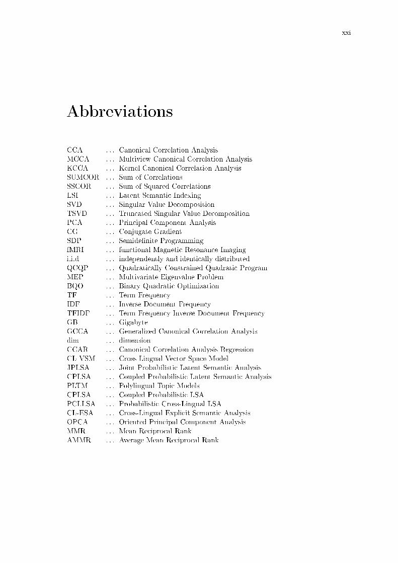
Abbreviations
CCA . . . Canonical Correlation AnalysisMCCA . . . Multiview Canonical Correlation AnalysisKCCA . . . Kernel Canonical Correlation AnalysisSUMCOR . . . Sum of CorrelationsSSCOR . . . Sum of Squared CorrelationsLSI . . . Latent Semantic IndexingSVD . . . Singular Value DecompositionTSVD . . . Truncated Singular Value DecompositionPCA . . . Principal Component AnalysisCG . . . Conjugate GradientSDP . . . Semide�nite ProgrammingfMRI . . . functional Magnetic Resonance Imagingi.i.d . . . independently and identically distributedQCQP . . . Quadratically Constrained Quadratic ProgramMEP . . . Multivariate Eigenvalue ProblemBQO . . . Binary Quadratic OptimizationTF . . . Term FrequencyIDF . . . Inverse Document FrequencyTFIDF . . . Term Frequency Inverse Document FrequencyGB . . . GigabyteGCCA . . . Generalized Canonical Correlation Analysisdim . . . dimensionCCAR . . . Canonical Correlation Analysis RegressionCL-VSM . . . Cross-Lingual Vector Space ModelJPLSA . . . Joint Probabilistic Latent Semantic AnalysisCPLSA . . . Coupled Probabilistic Latent Semantic AnalysisPLTM . . . Polylingual Topic ModelsCPLSA . . . Coupled Probabilistic LSAPCLLSA . . . Probabilistic Cross-Lingual LSACL-ESA . . . Cross-Lingual Explicit Semantic AnalysisOPCA . . . Oriented Principal Component AnalysisMMR . . . Mean Reciprocal RankAMMR . . . Average Mean Reciprocal Rank

xxiii
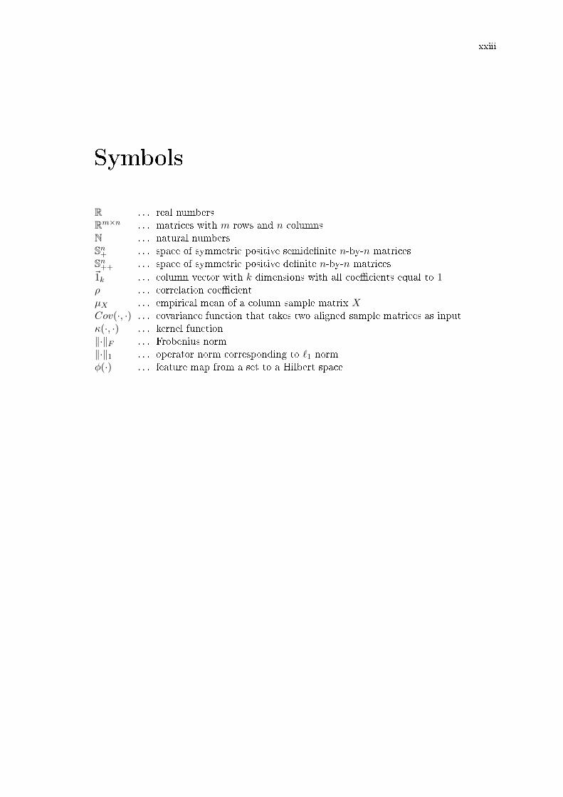
Symbols
R . . . real numbersRm×n . . . matrices with m rows and n columnsN . . . natural numbersSn+ . . . space of symmetric positive semide�nite n-by-n matricesSn++ . . . space of symmetric positive de�nite n-by-n matrices~1k . . . column vector with k dimensions with all coe�cients equal to 1ρ . . . correlation coe�cientµX . . . empirical mean of a column sample matrix XCov(·, ·) . . . covariance function that takes two aligned sample matrices as inputκ(·, ·) . . . kernel function‖·‖F . . . Frobenius norm‖·‖1 . . . operator norm corresponding to `1 normφ(·) . . . feature map from a set to a Hilbert space

xxv
Glossary
Correlation coe�cient measures the degree of linear dependence between two univariaterandom variables.Canonical Correlation Analysis is a way of measuring the linear relationship between twomultidimensional variables.Principal Component Analysis is a dimensionality reduction technique based on maximiza-tion of variance.Singular Value Decomposition is a factorization of a real or complex matrix.Vector Space Model is a representation of textual data in a vector space, based on countingthe occurrences of words, which correspond to vector space dimensions.Latent Semantic Indexing is a text analysis technique based on the singular value decom-position of the corpus matrix.k-means Clustering is a grouping algorithm that groups objects according to their similar-ity.Symmetric positive semide�nite matrix is a symmetric matrix with nonnegative eigenval-ues.Semide�nite programming is a sub�eld of convex optimization concerned with the optimiza-tion of a linear objective function over the intersection of the cone of positive semide�nitematrices with an a�ne space.Dual Representation expresses vectors as linear combinations over the training set.Hilbert space is a vector space equipped with an inner product.Kernel functions provide a way to manipulate data as though it were projected into ahigher dimensional space.Kernel methods are a class of algorithms for pattern analysis, based on embeddings into aHilbert space.

1
Chapter 1
Introduction
Pattern analysis is the process of �nding structure or regularity in a set of data. Forexample, if each data instance represents a point in a vector space, we might be interestedin the following question: does the dataset lie in a lower dimensional subspace (does itadmit a more compact representation)? In this case, the subspace represents a pattern(structure or regularity) discovered in the data. Principal Component Analysis provides asolution to such a question.
This thesis deals with �nding patterns in datasets that exhibit a multi-view aspect:that is, for each instance of data there are two or more representations (views) available.We refer to such datasets as aligned (multi-view) datasets. As an example of a two-viewdataset, consider a dataset where each instance is represented by a visual image and atextual description. Another example is a parallel multi-lingual corpus, where given nlanguages, each data instance consists of n documents, one for each language and thedocuments are related by being translations of each other. The patterns that we areinterested in represent regularities within each view that have associated regularities inother views. For example, when dealing with text, a type of pattern that is often ofinterest is a distribution over words from a �xed vocabulary, referred to as a topic vector.Given a collection of documents in a single language, a typical problem is to �nd relevanttopic vectors that summarize the document collection. The multi-view variant of theproblem then corresponds to �nding sets of multiple representations of topic vectors (oneper language). Methods that extract such multi-representation patterns represent the mainsubject of the thesis.
There are several possible applications of such an analysis. The patterns themselvescan be of interest for explorative analysis. For example, given an aligned dataset of fMRIbrain scans and visual images that were shown to the subjects as scans were taken, we caninvestigate how the brain functions by looking at relationships between brain activationregions and patterns in visual images. Another example of application is to use the multi-view patterns as maps into a representation independent space. For example, representingvisual images and textual descriptions in the same space can be used for cross-modalinformation retrieval, where one searches for images relevant to a query text, (or documentsrelevant to a given image) by using standard information retrieval techniques. In addition,the optimization problem related to one of the generalizations of Canonical CorrelationAnalysis (CCA) that we study appears in applications that range from control theory,blind source separation to multiple subject fMRI analysis.
2 Chapter 1. Introduction
1.1 Overview and Questions Addressed
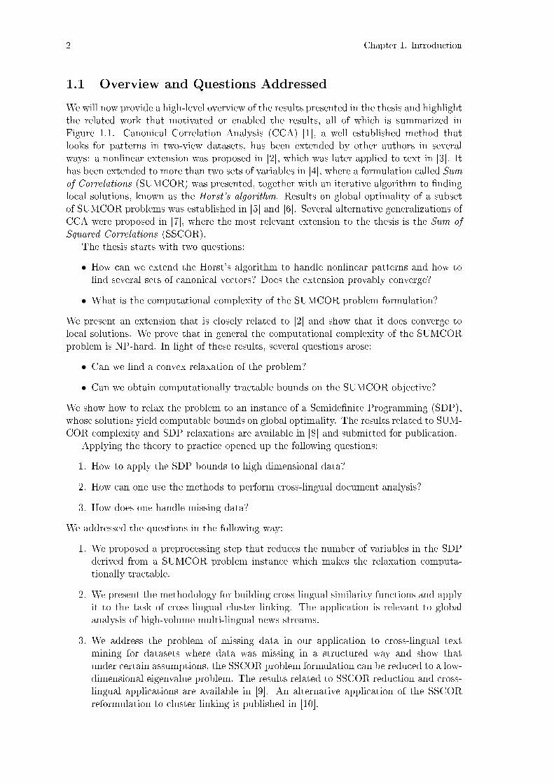
We will now provide a high-level overview of the results presented in the thesis and highlightthe related work that motivated or enabled the results, all of which is summarized inFigure 1.1. Canonical Correlation Analysis (CCA) [1], a well established method thatlooks for patterns in two-view datasets, has been extended by other authors in severalways: a nonlinear extension was proposed in [2], which was later applied to text in [3]. Ithas been extended to more than two sets of variables in [4], where a formulation called Sumof Correlations (SUMCOR) was presented, together with an iterative algorithm to �ndinglocal solutions, known as the Horst's algorithm. Results on global optimality of a subsetof SUMCOR problems was established in [5] and [6]. Several alternative generalizations ofCCA were proposed in [7], where the most relevant extension to the thesis is the Sum of
Squared Correlations (SSCOR).The thesis starts with two questions:
• How can we extend the Horst's algorithm to handle nonlinear patterns and how to�nd several sets of canonical vectors? Does the extension provably converge?
• What is the computational complexity of the SUMCOR problem formulation?
We present an extension that is closely related to [2] and show that it does converge tolocal solutions. We prove that in general the computational complexity of the SUMCORproblem is NP-hard. In light of these results, several questions arose:
• Can we �nd a convex relaxation of the problem?
• Can we obtain computationally tractable bounds on the SUMCOR objective?
We show how to relax the problem to an instance of a Semide�nite Programming (SDP),whose solutions yield computable bounds on global optimality. The results related to SUM-COR complexity and SDP relaxations are available in [8] and submitted for publication.
Applying the theory to practice opened up the following questions:
1. How to apply the SDP bounds to high dimensional data?
2. How can one use the methods to perform cross-lingual document analysis?
3. How does one handle missing data?
We addressed the questions in the following way:
1. We proposed a preprocessing step that reduces the number of variables in the SDPderived from a SUMCOR problem instance which makes the relaxation computa-tionally tractable.
2. We present the methodology for building cross-lingual similarity functions and applyit to the task of cross-lingual cluster linking. The application is relevant to globalanalysis of high-volume multi-lingual news streams.
3. We address the problem of missing data in our application to cross-lingual textmining for datasets where data was missing in a structured way and show thatunder certain assumptions, the SSCOR problem formulation can be reduced to a low-dimensional eigenvalue problem. The results related to SSCOR reduction and cross-lingual applications are available in [9]. An alternative application of the SSCORreformulation to cluster linking is published in [10].
1.2. Scienti�c Contributions 3
Canonical Correlation
Analysis (Hotelling)
Kernel Canonical Correlation
Analysis (Bach et. al.)
SUMCOR generalization (Horst) SSCOR generalization
(Kettenring)
Global optimality
results of SUMCOR
(Zhang et. al.)
Subset of SSCOR problems
reduced to eigenvalue problems [9]
Application of SUMCOR and SSCOR to Cross-Lingual Document Analysis [8][9]
Application to Cross-Lingual Cluster
Linking [9][10]
Application to Bi-Lingual
Document Analysis (Vinokourov et. al.)
Kernelized Multdimensional
Horst Algorithm [8]SUMCOR NP-
Hard [8]
SUMCOR SDP relaxation [8]
Tractable global
optimality bounds [8]
SUMCOR SDP +
random projections [8]
Horst algorithm (Horst)
Application to Cross-Lingual Information
Retrieval [9]
Theory
Applications
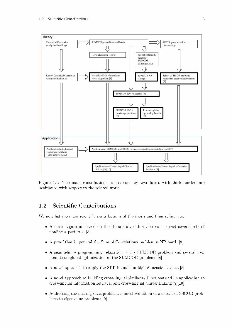
Figure 1.1: The main contributions, represented by text boxes with thick border, arepositioned with respect to the related work.
1.2 Scienti�c Contributions
We now list the main scienti�c contributions of the thesis and their references:
• A novel algorithm based on the Horst's algorithm that can extract several sets ofnonlinear patterns [8]
• A proof that in general the Sum of Correlations problem is NP-hard [8]
• A semide�nite programming relaxation of the SUMCOR problem and several newbounds on global optimization of the SUMCOR problems [8]
• A novel approach to apply the SDP bounds on high-dimensional data [8]
• A novel approach to building cross-lingual similarity functions and its application tocross-lingual information retrieval and cross-lingual cluster linking [9][10]
• Addressing the missing data problem, a novel reduction of a subset of SSCOR prob-lems to eigenvalue problems [9]

4 Chapter 1. Introduction
1.3 Thesis Structure
The rest of the thesis is structured as follows. Chapter 2 introduces notation and somede�nitions. For background we describe three pattern analysis methods that are the mostrelevant for the thesis and explain how they can be adapted for analysis of nonlinearpatterns in Chapter 3. Chapter 4 introduces a central problem of the thesis: generalizationsof Canonical Correlation Analysis (CCA) and the original contributions that extend themethod to nonlinear and higher-dimensional setting. In Chapter 5 we prove the result onthe complexity of a particular generalization and study global optimality guarantees basedon semide�nite relaxations. Chapter 6 discusses an application of multiview learning tobuilding cross-lingual similarity models. We show how a particular structure of the datacan be exploited to express a particular generalization of CCA as an eigenvector problem.Chapter 7 then shows how the cross-lingual similarity measures can be used to performcross-lingual cluster linking, relevant for large scale monitoring of global news in multiplelanguages. In Chapter 8 several experiments are presented both on synthetic and realdatasets. Finally, Chapter 9 concludes the thesis and discusses possible future directions.
5
Chapter 2
Notation and De�nitions
We �rst introduce the notation we use throughout the thesis:
• Column vectors are denoted by lowercase letters, e.g. x and matrices are denoted byuppercase letters, e.g. X.
• Subscripts are used to enumerate vectors or matrices, e.g. x1, x2, X1, except in thespecial case of the identity matrix, In and the zero matrix 0k,l. In these cases, thesubscripts denote row and column dimensions.
• We use superscripted symbol T for vector and matrix transpose, e.g. xT .
• Let ‖v‖ or ‖v‖2 denote the `2 norm of the vector v and let ‖A‖F , ‖A‖1 and ‖A‖2denote the Frobenius norm and the operator norms induced by 1-norm and 2-normrespectively.
• MATLAB notation [11]
� The i-th element of vector x is denoted by x(i) and the matrix entry in the i-throw and j-th column is denoted by X(i, j).
� The i-th row of matrix X is denoted by X(i, :) and the j-th column by X(:, j).matrix elements, rows and columns (e.g. X(i, j), X(i, :), X(:, j))
� Matrix concatenation: [A B] represents horizontal concatenation and [A;B]represents vertical concatenation.
� diag(v) denotes a diagonal matrix whose diagonal entries correspond to vectorv.
� 1k denotes a column vector with k elements all equal to 1.
• Spaces
� Rn denotes the n-dimensional real vector space.
� Rn×m denotes the (n ·m)-dimensional vector space used when specifying matrixdimensions.
� N denotes the natural numbers.
� Sn+ denotes the space of symmetric positive semide�nite n-by-n matrices.
� Sn++ denotes the space of symmetric positive de�nite n-by-n matrices.
• Random vectors are denoted by calligraphic letters, e.g. X and X ∈ Rn denotes theirdimension.

6 Chapter 2. Notation and De�nitions
2.1 Sample Datasets and the Multiview Assumption
The following de�nitions will be relevant for our discussion of kernel versions of the methodsrelevant to this thesis.
De�nition 2.1. A sample dataset with ` samples and n dimensions is a set
S := {x1, . . . , x`},where xi ∈ Rn are generated independently and identically distributed (i.i.d.) accordingto an underlying distribution.
De�nition 2.2. A n × ` sample matrix based on a dataset S with ` samples and ndimensions is obtained by horizontally concatenating the samples:
X := [x1 · · ·x`] .De�nition 2.3. A multiview sample dataset with ` samples and m views is a set:
S ={(
x(1)1 , . . . , x
(m)1
), . . . ,
(x(1)` , . . . , x
(m)`
)},
where x(j)i ∈ Rnj corresponds to the j-th view of the i-th sample. We assume that eachsample point was generated independently and identically distributed (i.i.d.) according toan underlying distribution with a speci�c structure. We assume that the samples representdi�erent views of an underlying object, that is, the observed random vectors are functionsof an unobserved random vector:(
X (1), . . . ,X (m))
= (f1(O), . . . , fm(O)) .
De�nition 2.4. Given a multiview dataset S with ` samples and m views, we form amatrix for view i by using horizontal concatenation:
Xi :=[x(i)1 · · ·x
(i)`
].
We refer to the set {X1, . . . , Xm} as multiview aligned matrices.In general, we will say that two matrices are aligned, if their columns form observation
vector pairs, related to a multiview dataset.
De�nition 2.5. A multiview stacked matrix based on a dataset S with ` samples and mviews is a matrix obtained by vertically concatenating the multiview aligned matrices:
X := [X1; · · · ;Xm] .
De�nition 2.6. The sample matrix is centered if its rows sum to zero.
De�nition 2.7. Given a n×` sample matrix X, the empirical mean µX ∈ Rn is computedas:
µX(i) =1
`
∑
j
X(i, j).
De�nition 2.8. Given a sample matrix X ∈ Rn×` the empirical covariance is de�ned as:
Cov(X) :=1
n− 1(X − µX ·~1T` ) · (X − µX ·~1T` )T .
De�nition 2.9. Empirical variance V ar(X) is de�ned as the empirical covariance forsingle dimensional sample matrices, that is, when n equals 1.
De�nition 2.10. Given two aligned sample matrices X1 ∈ Rn1×` and X2 ∈ Rn2×` theempirical cross-covariance is de�ned as:
Cov(X1, X2) :=1
n− 1(X1 − µX1 ·~1T` ) · (X2 − µX2 ·~1T` )T .

2.2. Kernel Methods 7
2.2 Kernel Methods
The following de�nitions will be relevant for our discussion of kernel versions of the methodsrelevant to this thesis. For de�nitions of standard concepts from topology we refer thereader to standard texts [12].
De�nition 2.11. A metric space is an ordered pair (M,d), where M is a set and d :M ×M → R is a metric on M , i.e., a function which satis�es for all x, y, z ∈M :
1. d(x, y) ≥ 0,
2. d(x, y) = 0⇐⇒ x = y,
3. d(x, y) = d(y, x),
4. d(x, z) ≤ d(x, y) + d(y, z).
De�nition 2.12. Let X be a metric space equipped with a metric d : X × X → R. Asequence (x1, x2, x3, . . .) is a Cauchy sequence, if for every ε > 0 there exists a positiveinteger N such that for all m,n > N :
d(xm, xn) < ε.
De�nition 2.13. A metric space X is complete, if every Cauchy sequence of elements inX converges to an element of X.
De�nition 2.14. A topological spaceH is separable if it contains a countable dense subset;that is, there exists a sequence (xn)∞n=1 such that every nonempty open subset of the spacecontains at least one element of the sequence.
De�nition 2.15. A Hilbert space H is an inner product space that is both separable andcomplete.
De�nition 2.16. Let V ⊂ Rn. A kernel is a function κ : V × V → R that satis�es:
κ(x, y) = 〈φ(x), φ(y)〉, ∀x, y ∈ V,
where φ : V → H is a function from V to a Hilbert space.
De�nition 2.17. Given a sample matrix X ∈ Rn×` and a kernel function κ, we de�ne akernel matrix K ∈ R`×` as:
K(i, j) := κ(xi, xj).
A special case of a kernel matrix is the Gram matrix, where the standard inner productis used as the kernel function (also referred to as the linear kernel).
De�nition 2.18. A matrix A is positive semide�nite if:
xTAx ≥ 0, ∀x.
The space of positive semide�nite matrices is denoted by S+.
De�nition 2.19. A matrix A is positive de�nite if:
xTAx > 0, ∀x.
The space of positive de�nite matrices is denoted by S++.

9
Chapter 3
Background
The central subjects in the thesis revolve around statistical approaches to �nding structurein one, two or more sets of variates. We will introduce two methods that �nd structure ina single set of variates: k-means clustering and Singular Value Decomposition (SVD) fordimensionality reduction, which is closely related to Principal Component Analysis (PCA).We will then present Canonical Correlation Analysis (CCA), a method for studying twosets of variates. We will also brie�y cover kernel method extensions of the methods andpresent some results on Semide�nite Programming.
3.1 k-means Clustering
The k-means algorithm [13] is perhaps the most well-known and widely-used clusteringalgorithm. In spirit of analysis on multiview methods that is to be presented, we willformulate k-means as a matrix factorization problem. Given an n× ` sample matrix (Def-inition 2.2) the goal is to �nd the best rank k approximation under additional constraints:
minimizeC∈Rn×k,P∈R`×k
‖X − C · P T ‖2F ,
subject to P (i, j) ∈ {0, 1}, ∀i, j∑
j
P (i, j) = 1, ∀i.(3.1)
The interpretation of the additional constraints on matrix P is that they force eachsample vector (column in X) to select precisely one column of C to approximate it andthe objective function corresponds to minimizing a sum of squared errors made by approx-imating points with centroids.
The matrix C in Equation 3.1 is uniquely de�ned for a given P , since for any given setof points in Rn, the point that minimizes the sum of squared distances to the set is themean. Since each column of P selects a subset of columns of X, C can be expressed as:
C := X · Pdiag(~1T` · P )−1P T , (3.2)
where the inverse of the diagonal matrix corresponds to division by the set size whencomputing the mean (~1T` ·P counts the number of points assigned to each of the k clusters).In addition, given C, the assignment P that minimizes the sum of squared errors can befound by:
P (i, j∗) = 1, where j∗ = arg minj‖X(:, i)− C(:, j)‖ (3.3)
A popular approach [13] to solving the problem in Equation 3.1 is to start with an initialassignment and alternate between updating C given P and vice versa. The approach is

10 Chapter 3. Background
widely used in practice, even though it is susceptible to �nding local minima. In general,the problem is known to be NP-hard [14].
3.2 Singular Value Decomposition
The second factorization based approach that is relevant to our work is based on theTruncated Singular Value Decomposition [11] (TSVD). It is closely related to PrincipalComponent Analysis [15] (PCA), a well established approach to dimensionality reduction.
Given an n× ` sample matrix (De�nition 2.2) the goal is to �nd a best approximationwith rank at most k under additional constraints:
minimizeU∈Rn×k,S∈Rk×k,V ∈R`×k
‖X − U · S · V T ‖F ,
subject to UTU = Ik
V TV = Ik
S = diag(σ), σ ∈ Rk, σ(i) ≥ 0.
(3.4)
The method of PCA is based on a low rank decomposition of the empirical covariancematrix, computed based on the sample matrix. The main idea is to �nd a subspace thataccounts for as much as variability in the data as possible. The �rst principal componentis de�ned as the one-dimensional subspace that maximizes the variance of the data whenprojected onto it. Formally, it solves the following problem:
maximizeu∈Rn
Var(uT ·X),
subject to ‖u‖ = 1.(3.5)
The other principal vectors can be obtained by de�ation [16], or equivalently solvingthe eigenvalue problem:
minimizeU∈Rn×k
‖Cov(X)− U · Λ · UT ‖F ,
subject to UTU = Ik
Λ = diag(λ), λ ∈ Rk.
(3.6)
One of the main applications of PCA is as a dimensionality reduction technique, wherethe data is projected to the space spanned by the normalized eigenvectors (also calledprincipal vectors). In typical applications a truncated eigenvalue decomposition is used,where one discards the principal vectors with small eigenvalues (similar to truncated SVDs).
If the data matrix is centered, then the solution U of TSVD and the eigenvector basisU of PCA will coincide.
3.3 Canonical Correlation Analysis
Canonical Correlation Analysis (CCA) [1] is a general procedure for studying relationshipsbetween two sets of random variables. It is based on analyzing the cross-covariance matrixbetween two random vectors with the aim of identifying linear relationships between them.We will start with intuitions and then give a formal presentation.
Roughly speaking, given two random vectors X (1) and X (2) we are interested in �non-trivial� pairs of functions (f (1), f (2)) such that there is a �dependence� between f (1)(X (1))and f (2)(X (2)). The �dependence� we consider is linear (possibly in a Hilbert space). The�non-triviality� of the functions is a requirement that guards us against trivial solutions,
3.3. Canonical Correlation Analysis 11
such as f (1)(x) := 0 · x, f (2)(y) := 0 · y - that is, f (1)(X (1)) and X (1) should share someinformation, and analogously for f (2)(X (2)) and X (2). In other words, f (1) and f (2) shouldnot destroy the original signals. When we are interested in more than one good pairof functions, for instance, a family of pairs (f
(1)i , f
(2)i ), we typically require additional
constraints to prevent non-trivial solutions by enforcing that f (1)i
(X (1)
)and f (1)j 6=i
(X (1)
)
share no information, and similarly for f (2)i . We are interested in essentially di�erentfunction pairs.
There are several possible applications of such an analysis. For example, a commonscenario involves analyzing objects o ∈ O, where O is some underlying space, which are notdirectly observable, but are only observable as images of transformations F (1) : O → Rp andF (2) : O → Rq. That is, we do not have access to o but only to
(F (1)(o), F (2)(o)
). Then
�nding function pairs (f(1)i , f
(2)i ) so that f (1)i (F (1)(o)) behave similarly as f (2)i (F (2)(o))
can be interpreted as �nding coupled parametrizations of image spaces of F (1) and F (2)
which agree on O. This enables applications such as cross-modal information retrieval,classi�cation, clustering, etc. If F (1) encodes a visual image and F (2) encodes a textualdescription of the scene, we can perform text input based search over a collection of images,see [17]. Bi-lingual document analysis is another application, see [3], [18]. The patternfunctions (f
(1)i , f
(2)i ) themselves can be interesting to study for exploratory purposes.
Formally, let
S = {(F (1)(o1), F
(2)(o1)), . . . ,
(F (1)(on), F (2)(on)
)}
represent a sample of n pairs drawn independently at random according to the under-lying distribution, where F (1)(xi) ∈ Rp and F (2)(xi) ∈ Rq represent feature vectorsfrom p and q-dimensional vector spaces. Let X(1) = [F (1)(o1), . . . , F
(1)(on)] and letX(2) = [F (2)(o1), . . . , F
(2)(on)] be the matrices with observation vectors as columns (usingMATLAB notation).
The idea is to �nd two vectors w(1) ∈ Rp and w(2) ∈ Rq so that the random variablesw(1)T · X (1) and w(2)T · X (2) are maximally correlated (w(1)T and w(2)T map the randomvectors to random variables, by computing weighted sums of vector components). By usingthe sample matrix notation X(1) and X(2) this problem can be formulated as the followingoptimization problem:
maximizew(1)∈Rp,w(2)∈Rq
w(1)TCov(X(1), X(2))w(2)
√w(1)TCov(X(1))w(1)
√w(2)TCov(X(2))w(2)
, (3.7)
where Cov(X(1)) and Cov(X(2)) are empirical estimates of variances of X (1) and X (2)
respectively and Cov(X(1), X(2)) is an estimate for the covariance matrix as de�ned inDe�nition 2.8 and De�nition 2.10. The optimization problem can be reduced to a gener-alized eigenvalue problem [17]:
[0 Cov(X(1), X(2))
Cov(X(2), X(1)) 0
]·[w(1)
w(2)
]=
λ ·[Cov(X(1), X(1)) 0
0 Cov(X(2), X(2))
]·[w(1)
w(2).
](3.8)
If the matrices Cov(X(1)) and Cov(X(2)) are not invertible, the problem is ill posed.One can use a regularization technique by replacing Cov(X(1)) with (1−τ)Cov(X(1))+τI,where τ ∈ [0, 1] is the regularization coe�cient and I is the identity matrix (and analo-gously for Cov(X(2))), see [16] for details. A single canonical variable is usually inadequate

12 Chapter 3. Background
in representing the original random vector and typically one looks for k projection pairs(w
(1)1 , w
(2)1 ), . . . , (w
(1)k , w
(2)k ), so that w(1)
i and w(2)i are highly correlated and w(1)
i is uncor-
related with w(1)j for j 6= i and analogously for w(2).
The formulation in Equation 3.8 can be reformulated as a symmetric eigenvalue prob-lem and solved e�ciently. In case the dimensions of the problem p and q are large andobservation vectors are sparse, one can consider an iterative method, for example Lanczosalgorithm [19]). Alternatively, if the number of observation vectors n is not prohibitivelylarge, one can reformulate the problem to its dual representation which can be combinedwith a �kernel trick� [2] to yield nonlinear version of CCA, which will be discussed in thenext section.
3.4 Kernel Methods
The methods discussed so far looked for patterns expressed in the same space as the sampledataset. We now discuss how we can extend the methods to �nding nonlinear patternsby using the framework of kernel methods. To look for nonlinear patterns in the originalspace, one �rst uses a nonlinear map φ to map the input data into a Hilbert space, wherelinear patterns are then extracted. If the Hilbert space is high dimensional the strategymight be computationally intractable. Let φ denote a feature map and κ its kernel functionas de�ned in De�nition 2.16, that is:
κ(x, y) = 〈φ(x), φ(y)〉.
If evaluating the kernel is feasible, then certain methods can be solved e�ciently, even ifφ is a map to an in�nite dimensional space. If in a given method the data and modelparameters interact only through inner products, then we can attempt to reformulate theproblem in terms of kernel matrices.
The general approach to kernelization of a method is to try to express the solutionin a dual basis, that is, the basis spanned by the training instances. The following twotheorems provide an alternative characterization of kernels and relate the kernel functionswith implicit feature maps. For an extended treatment of the concepts and the proofs werefer the reader to [16].
Theorem 3.1. A function κ : X × X → R, which is either continuous or has a �nite
domain, is a kernel function if and only if its kernel matrix is symmetric and positive
semide�nite on any �nite set of points.
Theorem 3.2. Given a kernel function κ : X × X → R we can reconstruct the implicit
Hilbert space H and the feature map φ as:
H := {k∑
i=1
αiκ(xi, ·) : k ∈ N, xi ∈ X},
φ(x) := κ(x, ·),
and the inner product is de�ned as:
〈φ(x), φ(y)〉 := κ(x, y).

3.4. Kernel Methods 13
3.4.1 Kernel k-means
Instead of working directly with columns of X we now work with φ (X(:, i)) for a φ thatcorresponds to a choice of kernel κ. Applying the iterative procedure described in Sec-tion 3.1 to the input space mapped by φ involves computing squared distances betweencolumns X(:, i) and centroids, which can be expressed as:
‖φ(X(:, i)− 1
|Sk|∑
j∈Sk
φ(X(:, j))‖2,
where Sk denotes the set of indices of points currently assigned to centroids k. Since‖x − y‖2 = 〈x − y, x − y〉 = 〈x, x〉 − 2〈x, y〉 + 〈y, y〉 the above quantity can be expressedusing kernel evaluations as:
κ (X(:, i), X(:, i))− 21
|Sk|∑
j∈Sk
κ (X(:, i), (X(:, j)) +1
|Sk|2∑
j,`∈Sk
κ (X(:, j), X(:, `)) .
Using Theorem 3.2, a new point x is mapped to κ(x, ·) and assigned the cluster thatminimizes
arg mink‖κ(x, ·)− 1
|Sk|∑
i∈Sk
κ (X(:, i), ·)‖2.
Again, computing the cluster assignment can be fully speci�ed through kernel evaluations.
3.4.2 Kernel PCA
We will assume that the data is centered to simplify presentation. The solution to PCAis expressed as an eigenvector decomposition of the covariance matrix. There is a directcorrespondence between the eigen-decompositions of the scaled covariance (`− 1)Cov(X)and the Gram matrix K = XTX. If (v, λ) is an eigenvector-eigenvalue pair for K, then(Xv, λ) is an eigenvalue pair for (`− 1)Cov(X):
(`− 1)Cov(X)Xv = XXTXv = XKv = λXv.
Since ‖Xv‖ =√vTXTXv =
√λvT v =
√λ, the solutions to the original problem are
expressed as linear combinations over the training examples of the form√λXv. Motivated
by this correspondence, the kernel methods approach thus analyzes the spectrum of thekernel matrix, given a kernel function.
Since the kernel matrix is symmetric and positive-de�nite, the eigenvectors form anorthonormal set in the Hilbert space and can thus be used as a projection. The normalizedeigenvector v (with an associated λ) is expressed in the Hilbert space:
√λ∑
i
v(i)φ(X(:, i))
which means that projecting a new point φ(x) in the kernel PCA coordinates is computedas:
P (φ(x))i :=√λ∑
i
v(i)κ(x,X(:, i)).
The centering assumption is not needed, as centering can be implemented as an oper-ation on the kernel matrix, as we will present in Section 4.4.3.
14 Chapter 3. Background
3.4.3 Kernel CCA
We will now present how to apply kernel methods to CCA and obtain the method knownas Kernel CCA (KCCA). The idea is to express the optimization problem in its dual form,where we express the solutions as linear combinations of their corresponding training in-stances. All the interactions with the data will be expressed through inner products, whichwill make the problem compatible with nonlinear feature maps based on their respectivekernels.
Let us express the vectors w(1) and w(2) in Equation 3.8 in their dual form by usingnew coordinate vectors α(1) ∈ R` and α(2) ∈ R` so that:
w(1) = X(1)α(1),
w(2) = X(2)α(2).
Assuming that the data is centered, the original optimization problem in Equation 3.9 isexpressed as:
maximizeα(1)∈R`, α(2)∈R`
α(1)TK(1)K(2)α(2)
√α(1)TK(1)K(1)α(1)
√α(2)TK(2)K(2)α(2)
. (3.9)
Applying the Lagrangian multiplier technique one can arrive at the dual form of thegeneralized eigenvalue problem:
[0 K(1)K(2)
K(2),K(1) 0
]·[α(1)
α(2)
]= (3.10)
λ ·[K(1)K(1) 0
0 K(2)K(2)
]·[α(1)
α(2).
](3.11)
To prevent over�tting, one can regularize the variances (1 − τ)Cov(X(1)) + τIp and(1 − τ)Cov(X(2)) + τIq. The corresponding regularized dual variances are expressed as:(1− τ)K(1)K(1) + τK(1) and (1− τ)K(2)K(2) + τK(2) can then replace the diagonal blocksof the right side of Equation 3.10.
3.5 Semide�nite programming
Semide�nite programming (SDP) problems are a subclass of convex optimization prob-lems that involve optimizing a linear function over the intersection of the cone of positivesemide�nite matrices with an a�ne space.
A primal SDP is given by:
minX∈Sn+
Tr (AX)
subject to Tr (BiX) = bi, ∀i = 1, . . . ,m.(3.12)
A dual SDP problem is closely related to the primal and is given by:
maxy∈Rm
〈b, y〉
subject to A−m∑
i=1
yiBi ∈ Sn.(3.13)
An important property of both problems is that they are convex (see [20]) which meansthat any locally optimal solution is also globally optimal. The following two theorems relatethe optimal objective values of primal and dual formulations. For proofs of the next twotheorems please refer to a standard textbook on convex optimization [20].

3.5. Semide�nite programming 15
Theorem 3.3 (Weak duality). Let X∗ denote the optimal solution to the problem 3.12
and y∗ the optimal solution to the problem 3.13. Then
Tr(AX∗)− 〈b, y∗〉 ≥ 0.
The di�erence between the objective values is referred to as the duality gap.
Theorem 3.4 (Strong duality). If the optimization problem 3.12 is bounded from below
(optimal solution X∗ to the problem 3.12 exists) and there exists X0 ∈ Sn++ such that
Tr(X0Bi) = bi, ∀i = 0, . . . ,m, (3.14)
then the optimal solution y∗ to the problem 3.13 exists and:
Tr(AX∗) = 〈b, y∗〉.
Not all SDP problems result in a zero duality gap, but as it will turn out, the problemsthat we will be interested in do. This is relevant from a practical perspective, since manymodern optimization SDP solvers, such as primal-dual interior point methods, convergeonly when the duality gap is zero.
We now present an important result that has been established [21] on the rank of SDPsolutions (relevant to Chapter 5).
Theorem 3.5. If there is an optimal solution for SDP, then there is an optimal solution
of SDP whose rank r satis�es:r(r + 1)
2< m.
There also exists a constructive version of the statement [22]. See [23, Chapter 6.5] fora proof.
Summary. This chapter introduced some well known data analysis techniques that playan important role in the following chapters. More concretely, CCA and KCCA serve as thebasis of our proposed extensions in Chapter 4, SVD and k-means are used as benchmarksfor cross-lingual document analysis in Chapter 8 and SVD is used as a preprocessing stepfor an original method that will be introduced in Chapter 6. The chapter also introducedSDP problems, which will be used to obtain global optimality results in Chapter 5.

17
Chapter 4
Nonlinear Multiview Canonical
Correlation Analysis
This chapter will discuss generalizations of CCA to analysis of multiple sets of variables.The problem is then known as the Multi-set Canonical Correlation Analysis (MCCA),or sometimes Multiview Canonical Correlation Analysis. Whereas it can be shown thatCCA can be solved using an (generalized) eigenvalue computation, MCCA is a muchmore di�cult problem. We will describe a generalization proposed in [7] and present aniterative locally optimal solution proposed in [4], referred to as the Horst's algorithm, whichrepresents a starting point of our work.
For use in practical applications, we propose a novel algorithm based on two originalcontributions of the Horst's algorithm: we adapt the methods to use kernels and to �ndmulti-dimensional solutions, analogous to �nding multiple principal directions in PCA andmultiple pairs of canonical vectors in CCA.
4.1 Related Work
CCA, introduced in Section 3.3, was developed to detect linear relations between two sets ofvariables. Typical uses of CCA include statistical tests of dependence between two randomvectors, exploratory analysis on multi-view data, dimensionality reduction and �nding acommon embedding of two random vectors that share mutual information.
CCA has been generalized in two directions: extending the method to �nding nonlinearrelations by using kernel methods [2][17] and extending the method to more than two setsof variables [7], which we presented in Section 3.4. Among several proposed generalizationsin [7] the most important for our work are the Sum of Correlations (SUMCOR) and Sum
of Squared Correlations (SSCOR) generalizations, where SUMCOR will be the main focusof the current chapter and Chapter 5 and SSCOR will be studied in Chapter 6.
There the goal is to project m sets of random variables to m univariate random vari-ables, which are pair-wise highly correlated on average 1. An iterative method to solve theSUMCOR generalization was proposed in [4] and the proof of convergence was establishedin [24]. In [24] it was shown that a generic SUMCOR problem admits exponentially manylocally optimal solutions. In [6] the authors identi�ed a subset of SUMCOR problems forwhich the iterative procedure converges to a global maximizer (Their results apply to non-negative irreducible quadratic forms). In Chapter 5 we will discuss results on the problemcomplexity and global optimality conditions.
1Given m univariate random variables, one can compute(m2
)correlation coe�cients, one for each pair
of variables.

18 Chapter 4. Nonlinear Multiview Canonical Correlation Analysis
}m∑i=1
ni = N
Cov(X )X
C(1,1)
nmn1 n2
n1
n2
nmC(m,m)
C(1,2)
C(2,1) C(2,2)
C(1,m)
C(2,m)
C(m,1) C(m,2)X (m)
X (2)
X (1)
Figure 4.1: The block structure of the random vector X and the corresponding covarianceblock structure.
This chapter will focus on the local iterative approach [4] with the aim of extendingit so it may be used in applications similar to KCCA. Here we show how the methodcan be extended to �nding non-linear patterns and �nding more than one set of canonicalvariates. Our work is related to [25] where a de�ation scheme is used together with theNewton method to �nd several sets of canonical variates. Our nonlinear generalization isrelated to [26], where the main di�erence lies in the fact that we "kernelized" the problem,whereas the authors in [26] worked with explicit nonlinear feature representation.
We now list some applications of the SUMCOR formulation. In [27] an optimizationproblem for multi-subject functional magnetic resonance imaging (fMRI) alignment is pro-posed, which can be formulated as a SUMCOR problem (performing whitening on eachset of variables). Another application of the SUMCOR formulation can be found in [25],where it is used for group blind source separation on fMRI data from multiple subjects.An optimization problem equivalent to SUMCOR also arises in control theory [28] in theform of linear sensitivity analysis of systems of di�erential equations.
4.2 Sum of Correlations
In this section we will discuss a generalization of CCA to more than two views, which �ndsa set of directions (one per view) which maximizes the average correlation (computed foreach pair of views).
We assume that we are given a centered random vector X ∈ RN as de�ned in De�ni-tion 2.3, where X is composed of m subsets of random variables referred to as views. Weassume that the indices of components of each set are contiguous, i.e. X is a concatenationof blocks that correspond to views.Additional Notation. Let m denote the number of blocks and N the total number ofvariables in X . Then
b := (n1, . . . , nm) ,m∑
i=1
b (i) = N,
encodes the number of elements in each of the block. We denote the corresponding sub-vectors as X (i) ∈ Rni (i-th block-row of vector X ) and the sub-matrices as C(i,j) ∈ Rni×nj
(i-th block-row, j-th block column of matrix C); see Figure 4.1. For example, in CCA,there are only two sets, so m = 2.
Formally, given w ∈ RN we de�ne m random variables Zi (one-dimensional projectionsof random block components of X ) as:
Zi :=
ni∑
j=1
X (i) (j)w(i) (j) = X (i)T · w(i).
4.2. Sum of Correlations 19
Let ρ (x, y) denote the correlation coe�cient between two random variables:
ρ (x, y) =Cov (x, y)√
Cov (x, x)Cov (y, y).
The correlation coe�cient between Zi and Zj can be expressed as:
ρ (Zi,Zj) =w(i)TC(i,j)w(j)
√w(i)TC(i,i)w(i)
√w(j)TC(j,j)w(j)
.
Initial Problem Formulation.The problem described above can be stated as �nding the set of vectors w(i) which
maximizem∑
i=1
m∑
j=i+1
ρ (Zi,Zj) . (SUMCOR)
We refer to this problem as Multi-set Canonical Correlation Analysis (MCCA). Note that itreduces to CCA whenm = 2. The solution - that is, the set of components
(w(1), . . . , w(m)
),
are referred to as the set of canonical vectors.Another formulation proposed in [7] is the Sum of Squared Correlations (SSCOR)
m∑
i=1
m∑
j=i+1
ρ (Zi,Zj)2 . (SSCOR)
The second formulation is invariant to the signs of the correlation coe�cients. It will beof importance in Chapter 6.Reformulating the Optimization Problem.
Expanding SUMCOR, we get:
maxw∈RN
m∑
i=1
m∑
j=i+1
w(i)TC(i,j)w(j)
√w(i)TC(i,i)w(i)
√w(j)TC(j,j)w(j)
.
Observe that the solution is invariant to block scaling (only the direction matters): if(w(1), . . . , w(m)
)is a solution, then
(α1 · w(1), . . . , αm · w(m)
)is also a solution for αi > 0.
We may therefore impose constraints w(i)TC(i,i)w(i) = 1, which only a�ect the norm. Thisyields the following equivalent constrained problem:
maximizew∈RN
m∑
i=1
m∑
j=i+1
w(i)TC(i,j)w(j)
subject to w(i)TC(i,i)w(i) = 1, ∀i = 1, . . . ,m.
(4.1)
We further multiply the objective by 2 and add a constant m. Note that this does nota�ect the optimal solution. Using the equalities: w(i)TC(i,j)w(j) = w(j)TC(j,i)w(i) andw(i)TC(i,i)w(i) = 1, we obtain:
maximizew∈RN
m∑
i=1
m∑
j=1
w(i)TC(i,j)w(j)
subject to w(i)TC(i,i)w(i) = 1, ∀i = 1, . . . ,m.
(4.2)
This transforms the objective function into a quadratic form wTCw. To simplify theconstraints, assume that C(i,i) is strictly positive de�nite. If C(i,i) is not full rank, thenusing the eigenvalue decomposition C(i,i) = V ΛV T , where V ∈ Rni×k, Λ ∈ Rni×k, Λ > 0,
20 Chapter 4. Nonlinear Multiview Canonical Correlation Analysis
k < ni, we substitute X (i) with V TX (i) ∈ Rk, for which the covariance matrix is strictlypositive de�nite.
From the strict positive de�niteness it follows that C(i,i) admits a Cholesky decompo-sition: there exists an invertible triangular matrix Di such that C(i,i) = DT
i Di.Finally, using the block structure b, we substitute w(i) with D−1i x(i) and de�ne A ∈ RN
as:A(i,j) := Di
−TC(i,j)Dj−1,
leading to the simpli�ed problem:
maxx∈RN
xTAx
subject to x(i)Tx(i) = 1, ∀i = 1, . . . ,m.(QCQP)
It turns out that (QCQP) is simpler to manipulate than (SUMCOR), so we use this formfrom this point on.
Using the technique of Lagrange multipliers (see [24]) we can relate the stationarypoints of the problem in Equation (QCQP) to solutions of a nonlinear system of equations:
m∑
j=1
A(i,j)x(i) = λix(i), ∀i = 1, . . . ,m, (4.3)
where λ1, . . . , λm ∈ R. This formulation is referred to as a Multivariate Eigenvalue Problem(MEP). The following theorem has been established [24].
Theorem 4.1. Consider the problem in Equation (4.3). If the matrix A is symmetric and
generic, then the number of solutions to the system is exactly
Πmi=12ni.
This means that in general the number of solutions grows exponentially with the num-ber of views. Notice however that A in Equation (QCQP) is not generic as each of theblocks on its diagonal is an identify matrix.
4.3 Local Solutions
In this section, we give an algorithm that converges to a locally optimal solution of theproblem (QCQP), when the matrix A is symmetric, positive-de�nite and generic (the proofwas established in [24]).
The algorithm can be interpreted as a generalization of the power iteration method (alsoknown as the Von Mises iteration), a classical approach to �nding the largest solutions tothe eigenvalue problem Ax = λx. The general iterative procedure is given as Algorithm 4.1.
In the case of m = 1, Algorithm 4.1 corresponds exactly to the power iteration. Whilethe algorithm's convergence to a local optimum is guaranteed, its convergence rate is notknown. In Chapter 8 we will examine the convergence rate on synthetic data.
4.4 Proposed Extensions
Here we present two extensions of MCCA: how to use kernel methods with MCCA to�nd nonlinear dependencies in the data; and an algorithm to �nding more than one set ofcorrelation vectors.
4.4. Proposed Extensions 21
Algorithm 4.1: Horst's algorithm
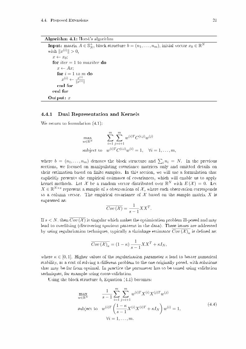
Input: matrix A ∈ S+N , block structure b = (n1, . . . , nm), initial vector x0 ∈ RNwith ‖x(i)‖ > 0,x← x0;for iter = 1 to maxiter dox← Ax;for i = 1 to m dox(i) ← x(i)
‖x(i)‖end for
end for
Output: x
4.4.1 Dual Representation and Kernels
We return to formulation (4.1):
maxw∈RN
m∑
i=1
m∑
j=i+1
w(i)TC(i,j)w(j)
subject to w(i)TC(i,i)w(i) = 1, ∀i = 1, . . . ,m,
where b = (n1, . . . , nm) denotes the block structure and∑
i ni = N . In the previoussections, we focused on manipulating covariance matrices only and omitted details ontheir estimation based on �nite samples. In this section, we will use a formulation thatexplicitly presents the empirical estimates of covariances, which will enable us to applykernel methods. Let X be a random vector distributed over RN with E (X ) = 0. LetX ∈ RN×s represent a sample of s observations of X , where each observation correspondsto a column vector. The empirical covariance of X based on the sample matrix X isexpressed as:
Cov (X ) =1
s− 1XXT .
If s < N , then Cov (X ) is singular which makes the optimization problem ill-posed and maylead to over�tting (discovering spurious patterns in the data). These issues are addressedby using regularization techniques, typically a shrinkage estimator Cov (X )κ is de�ned as:
Cov (X )κ = (1− κ)1
s− 1XXT + κIN ,
where κ ∈ [0, 1]. Higher values of the regularization parameter κ lead to better numericalstability, at a cost of solving a di�erent problem to the one originally posed, with solutionsthat may be far from optimal. In practice the parameter has to be tuned using validationtechniques, for example using cross-validation.
Using the block structure b, Equation (4.1) becomes:
maxw∈RN
1
s− 1
m∑
i=1
m∑
j=i+1
w(i)TX(i)X(j)Tw(j)
subject to w(i)T
(1− κs− 1
X(i)X(i)T + κIN
)w(i) = 1,
∀i = 1, . . . ,m.
(4.4)

22 Chapter 4. Nonlinear Multiview Canonical Correlation Analysis
To express each component w(i) in terms of the columns of X(i), let w have block structurebw = (n1, . . . , nm) where
∑i ni = N , and let y ∈ Rm·s have block structure by (i) = s, ∀i =
1, . . . ,m. The component w(i) can be expressed as:
w(i) =
s∑
j=1
y(i) (j)X(i) (:, j) = X(i)y(i). (4.5)
We refer to y as dual variables. Let Ki = X(i)TX(i) ∈ Rs×s denote the Gram matrix. Wecan now express the problem (4.4) in terms of the dual variables:
maxy∈Rm·s
1
s− 1
m∑
i=1
m∑
j=i+1
y(i)TKiKTj y
(j)
subject to y(i)T(
1− κs− 1
KiKTi + κKi
)y(i) = 1,
∀i = 1, . . . ,m.
(4.6)
Expressing the problem in terms of Gram matrices makes it amenable to using kernelmethods (see [16]). It remains to check that the formulations (4.4) and (4.6) are equivalent.
Lemma 4.2. There exists a solution to (4.4) which can be expressed as (4.5).
Proof. We prove the lemma by contradiction. Assume that no optimal solution can beexpressed as (4.5) and let u be an optimal solution to the problem (4.4). Without loss ofgenerality, assume that u(1) does not lie in the column space of X(1):
u(1) = z⊥ +X(1)y(1),
where
z⊥ 6= 0n1 and X(1)T z⊥ = 0s.
We show that u, de�ned as u(i) := u(i), ∀i > 1 and u(1) := 1γX
(1)y(1), where
γ :=
√y(1)TX(1)T
(1− κs− 1
X(1)X(1)T + κIN
)X(1)y(1),
strictly increases the objective function, which contradicts the assumption that u is optimal.Clearly, u is a feasible solution. Positive de�niteness of 1−κ
s−1X(1)X(1)T +κIN , coupled with
the fact that zT⊥z⊥ > 0, implies that 0 < γ < 1. Let E :=∑m
j=2
(X(1)y(1)
)TX(1)X(j)Tu(j).
If E < 0, then the vector [−u(1)T u(2)T · · · u(m)T ]T strictly increases the objectivefunction, which is a contradiction. We also obtain a contradiction if E = 0, since anynonzero v ∈ Rs for which X(1)v 6= 0n1 can be used to obtain a solution to the problem(4.4) expressed as (4.5) (after re-scaling such that Cov
(X (1)v
)κ
= 1 and if necessary
multiplying it by −1 so that∑m
j=2
(X(1)v
)TX(1)X(j)Tu(j) ≥ 0). Thus, we may assume
that E > 0.The following inequality completes the proof, since it shows that u increases the objec-
tive function:
4.4. Proposed Extensions 23
1
s− 1
m∑
j=2
u(1)TX(1)X(j)Tu(j)
=1
s− 1
m∑
j=2
(z⊥ +X(1)y(1)
)TX(1)X(j)Tu(j)
=1
s− 1
m∑
j=2
(X(1)y(1)
)TX(1)X(j)Tu(j)
<1
s− 1
m∑
j=2
1
γ
(X(1)y(1)
)TX(1)X(j)Tu(j).
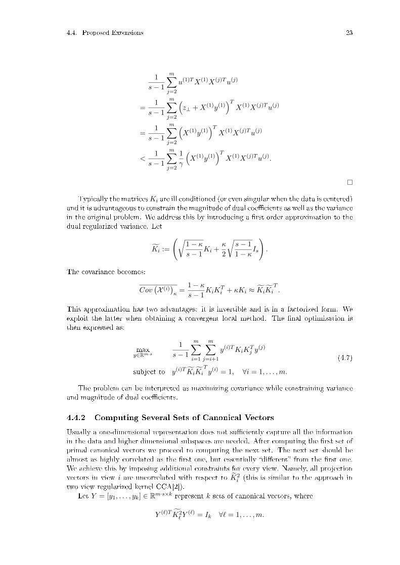
Typically the matricesKi are ill conditioned (or even singular when the data is centered)and it is advantageous to constrain the magnitude of dual coe�cients as well as the variancein the original problem. We address this by introducing a �rst order approximation to thedual regularized variance. Let
Ki :=
(√1− κs− 1
Ki +κ
2
√s− 1
1− κIs).
The covariance becomes:
Cov(X (i)
)κ
=1− κs− 1
KiKTi + κKi ≈ KiKi
T.
This approximation has two advantages: it is invertible and is in a factorized form. Weexploit the latter when obtaining a convergent local method. The �nal optimization isthen expressed as:
maxy∈Rm·s
1
s− 1
m∑
i=1
m∑
j=i+1
y(i)TKiKTj y
(j)
subject to y(i)T KiKiTy(i) = 1, ∀i = 1, . . . ,m.
(4.7)
The problem can be interpreted as maximizing covariance while constraining varianceand magnitude of dual coe�cients.
4.4.2 Computing Several Sets of Canonical Vectors
Usually a one-dimensional representation does not su�ciently capture all the informationin the data and higher dimensional subspaces are needed. After computing the �rst set ofprimal canonical vectors we proceed to computing the next set. The next set should bealmost as highly correlated as the �rst one, but essentially �di�erent� from the �rst one.We achieve this by imposing additional constraints for every view. Namely, all projectionvectors in view i are uncorrelated with respect to K2
i (this is similar to the approach intwo view regularized kernel CCA[2]).
Let Y = [y1, . . . , yk] ∈ Rm·s×k represent k sets of canonical vectors, where
Y (`)T K2` Y
(`) = Ik ∀` = 1, . . . ,m.
24 Chapter 4. Nonlinear Multiview Canonical Correlation Analysis
The equation above states that each canonical vector has unit regularized variance and thatdi�erent canonical vectors corresponding to the same view are uncorrelated (orthogonalwith respect to K2
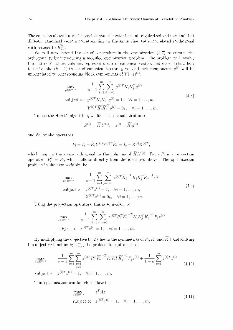
i ).We will now extend the set of constraints in the optimization (4.7) to enforce the
orthogonality by introducing a modi�ed optimization problem. The problem will involvethe matrix Y , whose columns represent k sets of canonical vectors and we will show howto derive the (k + 1)-th set of canonical vectors y whose block components y(i) will beuncorrelated to corresponding block components of Y (:, j)(i).
maxy∈Rm·s
1
s− 1
m∑
i=1
m∑
j=i+1
y(i)TKiKTj y
(j)
subject to y(i)T KiKiTy(i) = 1, ∀i = 1, . . . ,m,
Y (i)T KiKiTy(i) = 0k, ∀i = 1, . . . ,m.
(4.8)
To use the Horst's algorithm, we �rst use the substitutions:
Z(i) = KiY(i), z(i) = Kiy
(i)
and de�ne the operators
Pi = Is − KiY(i)Y (i)T Ki = Is − Z(i)Z(i)T ,
which map to the space orthogonal to the columns of KiY(i). Each Pi is a projection
operator: P 2i = Pi, which follows directly from the identities above. The optimization
problem in the new variables is:
maxz∈Rm·s
1
s− 1
m∑
i=1
m∑
j=i+1
z(i)T Ki−TKiK
Tj Kj
−1z(j)
subject to z(i)T z(i) = 1, ∀i = 1, . . . ,m,
Z(i)T z(i) = 0k, ∀i = 1, . . . ,m.
(4.9)
Using the projection operators, this is equivalent to:
maxz∈Rm·s
1
s− 1
m∑
i=1
m∑
j=i+1
z(i)TP Ti Ki−TKiK
Tj Kj
−1Pjz
(j)
subject to z(i)T z(i) = 1, ∀i = 1, . . . ,m.
By multiplying the objective by 2 (due to the symmetries of Pi,Ki and Ki) and shiftingthe objective function by m
1−κ , the problem is equivalent to:
maxz∈Rm·s
1
s− 1
m∑
i=1
m∑
j=1j 6=i
z(i)TP Ti Ki−TKiK
Tj Kj
−1Pjz
(j) +1
1− κm∑
i=1
z(i)T z(i)
subject to z(i)T z(i) = 1, ∀i = 1, . . . ,m.
(4.10)
This optimization can be reformulated as:
maxz∈Rm·s
zTAz
subject to z(i)T z(i) = 1, ∀i = 1, . . . ,m,(4.11)

4.4. Proposed Extensions 25
where A ∈ Rm·s with block structure b (i) = s, ∀i = 1, . . . ,m, is de�ned by:
A(i,j) =
1
s− 1P Ti Ki
−TKiK
Tj Kj
−1Pj for : i 6= j
1
1− κIs for : i = j
Lemma 4.3. The block matrix A de�ned above is positive de�nite (i.e. A ∈ Sm·s++).
Proof. A is symmetric, which follows from Pi = P Ti and Ki = KTi . Let z ∈ Rm·s. The
goal is to show that zTAz > 0. Let us de�ne an auxiliary matrix W as:
W =1
1− κm∑
i=1
z(i)TP Ti Ki−T ·
(κKi +
κ2 (s− 1)
4 (1− κ)Is
)Ki−1Piz
(i)
Each summand is positive-semide�nite, i.e. W ≥ 0 and W > 0 if ∃i : Piz(i) = z(i). What
follows is a sequence of inequalities, some of which must be strict, as will be established:
zTAz =1
s− 1
m∑
i=1
m∑
j=1j 6=i
z(i)TP Ti Ki−TKiK
Tj Kj
−1Pjz
(j)
+1
1− κm∑
i=1
z(i)T z(i) (4.12)
≥ 1
s− 1
m∑
i=1
m∑
j=1j 6=i
z(i)TP Ti Ki−TKiK
Tj Kj
−1Pjz
(j)
+1
1− κm∑
i=1
z(i)TP Ti Piz(i) (4.13)
=1
s− 1
m∑
i=1
m∑
j=1j 6=i
z(i)TP Ti Ki−TKiK
Tj Kj
−1Pjz
(j)
+1
1− κm∑
i=1
z(i)TP Ti Ki−TKi
TKiKi
−1Piz
(i) (4.14)
=1
s− 1
m∑
i=1
m∑
j=1j 6=i
z(i)TP Ti Ki−TKiK
Tj Kj
−1Pjz
(j)
+1
s− 1
m∑
i=1
z(i)TP Ti Ki−TKiK
Ti Ki
−1Piz
(i) +W (4.15)
= zTBBT z +W ≥ 0,
where B ∈ Rm·s×s, de�ned by B(i) = 1√s−1(KiKi
−1Pi)
T , with corresponding row blockstructure b (i) = s. The inequality after (4.12) holds since projection operators cannot
increase norms. (4.14) is equal to (4.13) using Ki−TKi
T= I. Regrouping the terms and
applying the de�nition of W , we obtain (4.15). The �nal equality follows, since the �rsttwo sums form a perfect square.
Now we will show that at least one of the two inequalities is strict. If Piz(i) 6= z(i) forsome i, then the �rst inequality is strict (‖Piz(i)‖ < ‖z(i)‖). Conversely, if Piz(i) = z(i) forall i, then W > 0, hence the last inequality is strict.

26 Chapter 4. Nonlinear Multiview Canonical Correlation Analysis
Matrix A has all the required properties for convergence, so we apply Algorithm 4.1.Solutions to (4.8) are obtained by back-substituting into y(i) = Ki
−1z(i).
The solution to the above problem can be found by solving the following problem:∑
j 6=iPiK
−1i KiKjK
−1j Pjαj +
1
(1− κ)2αi + λiαi = 0,∀i,
followed by multiplying the solutions αi by K−1i .Eigenvalue shifting techniques can be applied to enforce positive-de�niteness. The
algorithm is shown in Algorithm 4.2.
Algorithm 4.2: Horst's algorithm for computing a k-dimensional representationInput: K1, . . . ,Km, κ, maxiter, k,Output: Bk
1 , . . . , Bkm
Ki = (1− κ)Ki + κI, ∀ifor d = 1 to k doChoose random vectors α0
1, . . . , α0m
if d > 1 thenP di = I − KiB
d−1i Bd−1
i
′Ki
Set α0i ← P di α
0i , ∀i
elseP di = I ∀i
end ifu0i = KiK
−1i α0
i ,∀ifor i = 1 to maxiter dofor j = 1 to m do
αij ← P dj K−1j Kj
∑k 6=j u
i−1k +
(1
(1−κ)2
)αi−1j
αij ←αij√
αij′αij
uij ← KkK−1k αik
end forend forfor l = 1 to m doβdl = K−1l αmaxiterl
Bdl = [Bd
l , βdl ] if d > 1
Bdl = [βdl ] if d = 1
end forend for
4.4.3 Implementation
The algorithm requires matrix vector multiplications and inverted matrix vector multipli-cations. If the kernel matrices are products of sparse matrices: Ki = X(i)TX(i) with eachX(i) having s · n elements where s � n, then the kernel matrix vector multiplicationscost is 2ns rather than n2. Rather than computing the full inverses, we solve the systemKix = y for x, every time K−1i y is needed. Since regularized kernels are symmetric andmultiplying them with vectors is fast (roughly four times slower than multiplication withthe original sparse matrices X(i)), an iterative method like Conjugate Gradient (CG) [11]is suitable. Higher regularization parameters decrease the condition number of each Ki
which speeds up CG convergence.

4.4. Proposed Extensions 27
If we �x the number of iterations, maxiter, and number of CG steps, C, the compu-tational cost of computing a k-dimensional representation is upper bounded by: O
(C ·
maxiter · k2 · m · n · s), where m is the number of views, n the number of observations
and s average number of nonzero features of each observation. Since the majority of com-putations are sparse matrix-vector multiplications, the algorithm can be parallelized (thesparse matrices are �xed and can be split into multiple blocks).
So far, we have assumed that the data is centered. Centering can be implementedas a preprocessing step on the kernel matrix, or incorporated in the kernel matrix-vectormultiplication in order to exploit sparsity in the data. Let K := XTX denote the kerneland µ := 1
`X~1` denote the empirical mean of the column sample matrix X.
Kernel Matrix Centering. Computing the kernel on centered data is done as follows:
(X − µ~1T` )T (X − µ~1T` ) = XTX −~1`µTX −XTµ~1T` +~1`µTµ~1T`
= XTX − 1
`~1`~1
T` X
TX − 1
`XTX~1`~1
T` +
1
`
1
`~1`~1
T` (~1T` X
TX~1`)
= K − 1
`~1`(~1
T` K)− 1
`(K~1`)~1
T` +
~1T` K~1`
`2~1`~1
T` .
We see that if computing K is feasible, then the centering only involves a small setof steps with quadratic complexity, which include kernel-vector multiplication and addingrank 1 matrices to the kernel.Centering on the �y. If X ∈ RN×` is sparse, we cannot explicitly compute the kernelmatrix K, but we can perform fast matrix-vector multiplication as Kx = XT (Xx) isa sequence of two fast multiplications. We will now incorporate centering. Then X iscentered by subtracting the mean from each column, which in matrix notation correspondsto the matrix X − µ~1T` . Then, centering on the �y corresponds to computing:
(X − µ~1T` )T (X − µ~1T` )x = (X − µ~1T` )T (Xx− (~1T` x)µ)
= XT (Xx)− ((µTX)x)~1` − (~1T` x)(XTµ) + (~1T` x)(µTµ)~1`.
If the computation is dominated by XT (Xx), then centering on the �y is suitable forblack box matrix-vector based methods. Also note that µ, XTµ and (µTµ)~1` can bepre-computed.
Summary. This chapter presented two extensions of the SUMCOR problem and showedhow the Horst's algorithm can be modi�ed to �nd solutions of the extended formula-tions. The �rst extension is based on a dual representation of the optimization problemand enables looking for non-linear pattern analysis using kernel methods. The second ex-tension enables looking for more than one set of canonical vectors which enables �ndinghigher-dimensional projections of data into a common vector space. The next chapter willinvestigate the global optimality properties of the problem. Chapter 8 will provide someexperimental results.


29
Chapter 5
Relaxations and Bounds
The current chapter focuses on the optimization aspect of the SUMCOR problem. Wepresent our results on the computational complexity of the SUMCOR problem formulation,as well as several global optimality bounds.
5.1 NP-Hardness
In this section, we prove that the optimization problem QCQP is not only non-convex butNP-hard in general. We present a reduction from a general binary quadratic optimizationproblem.
Let A ∈ Rm×m. The binary quadratic optimization problem (BQO) is stated as:
maxx∈Rm
xTAx
subject to x (i)2 = 1, ∀i = 1, . . . ,m.(BQO)
Many hard combinatorial optimization problems (e.g. the maximum cut problem and themaximum clique problem [29]) can be reduced to BQO [30], which is known to be NP-hard.
We reduce a general instance of a BQO problem to an instance of the problem (QCQP).That means that despite the special structure of the problem (QCQP) (maximizing apositive-de�nite quadratic form over a product of spheres), it still falls into the class ofproblems that are hard (under the assumption that P 6= NP ). We begin with a generalinstance of BQO and through a set of simple transformations, obtain a speci�c instanceof (QCQP), with a block structure b = (1, . . . , 1). More concretely, we will show thatany BQO is equivalent to a BQO problem whose assoicated matrix is a correlation matrix(positive de�nite with ones on the diagonal), which is an instance of a the problem (QCQP.
Consider a BQO with a corresponding generic matrix A ∈ Rm×m. Since xTAx =
xT(A+AT )
2 x, we can assume that the matrix A is symmetric. The binary constraints implythat for any diagonal matrix D the quantity xTDx =
∑iD (i, i) is constant. This means
that for c > 0 large enough, we can replace the objective with an equivalent objectivexT (A+ c · I)x which is a positive-de�nite quadratic form. Setting c := ‖A‖1+1 guaranteesthat A + c · I is positive de�nite, since it is strictly diagonally dominant. From now on,we assume that the matrix A in the BQO is symmetric and positive-de�nite. Let g =maxiA (i, i) and let D ∈ Rm×m be the diagonal matrix with elements D (i, i) = g−A (i, i).The BQO is then equivalent to
maxx∈Rm
xT(A+D)
gx
subject to x (i)2 = 1, ∀i = 1, . . . ,m.
(5.1)

30 Chapter 5. Relaxations and Bounds
The matrix (A+D)g is a correlation matrix since it is a symmetric positive-de�nite with
all diagonal entries equal to 1. The optimization problem corresponds to a problem ofmaximizing a sum of pairwise correlations between univariate random variables (usingblock structure notation: b (i) = 1, ∀i = 1, . . . ,m). This shows that even the simple case ofmaximizing the sum of correlations where the optimal axes are known and only directionsneed to be determined, is NP-hard.
With a �xed number of views, the complexity is polynomial, which follows from recentresults on the computational complexity of quadratic maps [31]. The degree of the poly-nomial is asymptotically equal to the product1
∏mi=1 ni, where ni is the dimensionality of
the i-th view. In many applications (text mining, fMRI analysis) where the ni's are large,the computational cost becomes prohibitive even with m = 3.
5.2 Semide�nite Programming Relaxation
The Horst's algorithm is scalable and often works well in practice (see Chapter 8). However,it may not converge to a globally optimal solution. We show how to use a relaxation of theproblem to obtain candidate solutions for the original problem. The relaxation transformsthe problem into a semide�nite program and we prove lower bounds which relates theextracted SDP solution quality and the optimal QCQP objective value. We also present aset of upper bounds on the optimal QCQP objective value in Section 5.3. These can serveas certi�cates of optimality (or closeness to optimality) for the local solutions (obtainedby the local iterative approach for example).
In this section, we relax the formulation QCQP to an SDP problem. Let A ∈ SN×N++ andB1, . . . , Bm ∈ §N×N+ be matrices which share the block structure b := (n1, . . . , nm) ,
∑i b (i) =
N . The blocks B(k,l)i ∈ Rnk×nl for i, k, l = 1, . . . ,m are de�ned as:
B(k,l)i :=
{Ini : k = i, l = i0k,l : otherwise
,
where Ini ∈ Rni×ni is an identity matrix and 0k,l ∈ Rk×l is a matrix with all entries equalto zero. Since xTAx = Tr
(AxxT
), (QCQP) can be rewritten as:
maxx∈Rn
Tr(AxxT
)
subject to Tr(Bixx
T)
= 1, ∀i = 1, . . . ,m.(QCQP2)
Substituting the matrix xxT with a positive semide�nite matrix X ∈ Sn+ constrainedto have rank one:
maximizeX∈Sn+
Tr (AX)
subject to Tr (BiX) = 1, ∀i = 1, . . . ,m
rank (X) = 1.
Omitting the rank-one constraint, we obtain a semi-de�nite program in standard form:
maxX∈Sn+
Tr (AX)
subject to Tr (BiX) = 1, ∀i = 1, . . . ,m.(SDP)
Remark. If the solution of the problem (SDP) is rank-one, i.e. X can be expressed asX = y · yT , then y is the optimal solution for (QCQP).
1The number of local solutions to our problem of interest is established in [24].

5.2. Semide�nite Programming Relaxation 31
Low Rank Solutions We use the solutions of the SDP relaxation to extract solutions tothe original QCQP problem. In the process, we obtain a bound which relates the globalSDP bound and the optimal value of QCQP, giving a measure of the quality of the extractedsolution. If the solution is rank-one, then the relaxation is exact. Here we consider thecase where the solutions are low rank (close to rank-one).
Let X∗ be a solution to (SDP) and x∗ be the solution to (QCQP). A straightforwardway to extract a feasible solution to the problem (QCQP) from X∗ is to project its leadingeigenvector to the set of constraints. The following inequality always holds:
Tr (AX∗) ≥ Tr(A · x∗ · x∗T
).
The quality of the solution depends on how loose this inequality is, or rather how closethe matrix X∗ is to rank-one (Proposition 5.3). These depend on the spectral propertiesof matrix X and matrix A.
The projection of a vector y ∈ RN , ‖y(i)‖ 6= 0 to the feasible set of (QCQP) is given bymap π (·) : RN → RN :
π (y) :=
(y(1)
‖y(1)‖ , . . . ,y(m)
‖y(m)‖
)T.
We require the following technical assumption:
Assumption 5.1. Let b = (n1, . . . , nm) denote the block structure and∑
i ni = N . LetX∗ be the solution to the problem (SDP). Let xk denote the k-th eigenvector of X∗. Theassumption is the following:
‖x(i)1 ‖ > 0,∀i = 1, . . . ,m.
Remark. The assumption ensures that the projection to the feasible set, π(·), is wellde�ned. In our experiments, this was always the case, but does not hold in general as onecan �nd counterexamples, for example, let m = 2 and de�ne:
A =
[1 00 1
], B1 =
[1 00 0
], B2 =
[0 00 1
].
All symmetric positive de�nite matrices that satisfy the constraints are of the form:
X =
[1 εε 1
],
where ε < 0, and attain the same value Tr (AX) = 2, which is thus optimal. Since thisalso holds for X = I where the leading eigenvector can be de�ned as x1 = [01]T , which isin contrast with the assumption. This counterexample has a speci�c structure: the zeroson the o�-diagonal of A make the views completely independent and the problem is insome sense a trivial multi-view problem. It is possible that the assumption holds underadditional conditions, for example, that the matrix is not block diagonalizable under theproblem's block structure.
The following lemma depends on the projection operator and thus relies on the as-sumption.
Lemma 5.2. Let b = (n1, . . . , nm) denote the block structure and∑
i ni = N . Let X∗
be the solution to (SDP) for which Assumption 5.1 holds. Let αi := 1
‖x(i)1 ‖. If X∗ can be
expressed as:X∗ = λ1x1x
T1 + λ2x2x
T2 ,

32 Chapter 5. Relaxations and Bounds
where ‖x1‖ = 1, ‖x2‖ = 1, 〈x1, x2〉 and λ1 > 1 > λ2, then
λ1 ≤ αiαj ≤λ1
1− λ2.
Proof. The constraints in problem (SDP) are equivalent to:
λ1‖x(i)1 ‖2 + λ2‖x(i)2 ‖2 = 1,∀i = 1, . . . ,m.
Since λ2 < 1 and ‖x(i)2 ‖2 ≤ 1, we see that 0 ≤ λ2‖x(i)2 ‖2 < 1. Consequently:
0 <1− λ2λ1
< ‖x(i)2 ‖2 ≤1
λ1.
From αi = 1
x(i)1
it follows that
√λ1 ≤ αi ≤
√λ1
1− λ2,
and �nally:
λ1 ≤ αiαj ≤λ1
1− λ2,∀i, j = 1, . . . ,m.
Proposition 5.3. Let b = (n1, . . . , nm) denote the block structure and∑
i ni = N . LetX∗ be the solution to (SDP) and x∗ be the solution to (QCQP). Let xk denote the k-theigenvector of X∗, αi := 1
‖x(i)1 ‖, ψ := Tr (AX∗), and φ := Tr
(A · x∗ · x∗T
). If X∗ can be
expressed asX∗ = λ1x1x
T1 + λ2x2x
T2 ,
where x1 and x2 have unit length and λ1 > 1 > λ2, then:
ψ − π (x1)T Aπ (x1) ≤
(1
1− λ2− 1
)m2 + λ2‖A‖2.
Proof. First we note that:ψ ≥ φ ≥ π (x1)
T Aπ (x1) .
We can expand the left hand side in terms of the two eigenvectors. Grouping the elementsby the vector terms and using basic manipulations we arrive at the result.
ψ − π (x1)T Aπ (x1) = λ1
∑i,j x
(i)T1 A(i,j)x
(j)T1
+λ2∑
i,j x(i)T2 A(i,j)x
(j)T2 −∑i,j αiαjx
(i)T1 A(i,j)x
(j)T1
≤ ∑i,j(λ1 − αiαj)x
(i)T1 A(i,j)x
(j)T1 + λ2‖A‖2
≤ −∑i,j(λ1 − αiαj) · |x(i)T1 A(i,j)x
(j)T1 |+ λ2‖A‖2
≤(
λ11−λ2 − λ1
)·∑i,j
1αiαj
+ λ2‖A‖2≤
(λ1
1−λ2 − λ1)· m2
λ1+ λ2‖A‖2
=(
11−λ2 − 1
)·m2 + λ2‖A‖2.
Remark. Proposition 5.3 is based on the assumption that the solution is of rank 2. Al-though the assumption is very speci�c, it holds in general for m = 3 which is a result ofTheorem 3.5.

5.3. Upper Bounds on QCQP 33
A similar bound can be derived for the general case, provided that the solution toproblem (SDP) is close to rank-one.
Proposition 5.4. Let b = (n1, . . . , nm) denote the block structure and∑
i ni = N . LetX∗ be the solution to the problem (SDP) and x∗ the solution to the problem (QCQP).Let xk denote the k-th eigenvector of X∗, αi := 1
‖x(i)1 ‖and ψ := Tr (AX∗). If X∗ can be
expressed asX∗ = λ1x1x
T1 + λ2x2x
T2 + · · ·+ λnxnx
Tn ,
where each xi has unit length and λ1 > 1 >∑
i=2,...,nλi, then:
ψ − π (x1)T Aπ (x1)
≤
1
1− ∑i=2,...,n
λi− 1
m2 +
∑
i=2,...,n
λi
‖A‖2.
5.3 Upper Bounds on QCQP
We now present several upper bounds on the optimal QCQP objective value based on thespectral properties of the QCQP matrix A. We then bound the values of the SDP solutionsand present two constant relative accuracy guarantees.L2 Norm Bound We show an upper bound on the objective of (QCQP) based on thelargest eigenvalue of the problem matrix A.
Proposition 5.5. The objective value of (QCQP) is upper bounded by m · ‖A‖2.
Proof. The problem (QCQP) remains the same if we add a redundant constraint xTx = mobtained by summing the constraints
∑mi=1
(x(i)Tx(i) − 1
)= 0. We then relax the problem
by dropping the original constraints to get:
maxx∈RN
xTAx
subject to xTx = m.(5.2)
Since ‖A‖2 = max‖x‖2=1xTAx, it follows that the optimal objective value of the problem
(5.2) equals m · ‖A‖2.
Bound on possible SDP objective values The next lemma establishes two simplebounds on the optimal value of the SDP problem.
Lemma 5.6. Let X∗ be the solution to the problem (SDP) and let ψ := Tr (AX∗). Then
m ≤ ψ ≤ m2.
Proof. Express X∗ as:X∗ =
∑
i=1,...,N
λixixTi ,
where each xi has unit length and λ1 ≥ . . . ≥ λN ≥ 0. The lower bound follows from thefact that ψ upper bounds the optimal objective value of problem (QCQP) which is lowerbounded by m. The lower bound corresponds to the case of zero sum of correlations.
To prove the upper bound, �rst observe that the constraints in (SDP) imply that∑i=1,...,N
λi = m. Let y ∈ RN and ‖y‖ = 1. Let z :=(‖y(1)‖, . . . , ‖y(m)‖
)T. Observe that
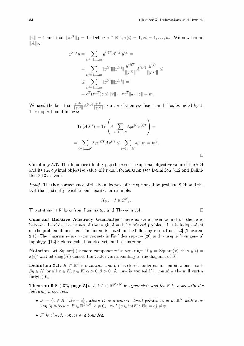
34 Chapter 5. Relaxations and Bounds
‖z‖ = 1 and that ‖zzT ‖2 = 1. De�ne e ∈ Rm, e (i) = 1, ∀i = 1, . . . ,m. We now bound‖A‖2:
yTAy =∑
i,j=1,...,m
y(i)TA(i,j)y(j) =
=∑
i,j=1,...,m
‖y(i)‖‖y(j)‖ y(i)T
‖y(i)‖A(i,j) y(j)
‖y(j)‖ ≤
≤∑
i,j=1,...,m
‖y(i)‖‖y(j)‖ =
= eT (zzT )e ≤ ‖e‖ · ‖zzT ‖2 · ‖e‖ = m.
We used the fact that y(i)T
‖y(i)‖A(i,j) y(j)
‖y(j)‖ is a correlation coe�cient and thus bounded by 1.The upper bound follows:
Tr (AX∗) = Tr
A
∑
i=1,...,N
λix(i)x(i)T
=
=∑
i=1,...,N
λix(i)TAx(i) ≤
∑
i=1,...,N
λi ·m = m2.
Corollary 5.7. The di�erence (duality gap) between the optimal objective value of the SDPand its the optimal objective value of its dual formulation (see De�nition 3.12 and De�ni-tion 3.13) is zero.
Proof. This is a consequence of the boundedness of the optimization problem SDP and thefact that a strictly feasible point exists, for example:
X0 := I ∈ SN++.
The statement follows from Lemma 5.6 and Theorem 3.4.
Constant Relative Accuracy Guarantee There exists a lower bound on the ratiobetween the objective values of the original and the relaxed problem that is independenton the problem dimension. The bound is based on the following result from [32] (Theorem2.1). The theorem refers to convex sets in Euclidean spaces [20] and concepts from generaltopology ([12]): closed sets, bounded sets and set interior.
Notation Let Square(·) denote componentwise squaring: if y = Square(x) then y(i) =x(i)2 and let diag(X) denote the vector corresponding to the diagonal of X.
De�nition 5.1. K ⊂ Rn is a convex cone if it is closed under conic combinations: αx +βy ∈ K for all x ∈ K, y ∈ K,α > 0, β > 0. A cone is pointed if it contains the null vector(origin) 0n.
Theorem 5.8 ([32, page 5]). Let A ∈ RN×N be symmetric and let F be a set with the
following properties:
• F = {v ∈ K : Bv = c} , where K is a convex closed pointed cone in RN with non-
empty interior, B ∈ Rk×N , c 6= 0k, and {v ∈ intK : Bv = c} 6= ∅.
• F is closed, convex and bounded.

5.3. Upper Bounds on QCQP 35
• There exists a componentwise strictly positive v ∈ F .Denote:
φ∗ = max{xTAx : square (x) ∈ F
},
φ∗ = min{xTAx : square (x) ∈ F
},
ψ∗ = max{
Tr (AX) : diag (X) ∈ F , X ∈ SN+},
ψ∗ = min{
Tr (AX) : diag (X) ∈ F , X ∈ SN+},
ψ (α) = αψ∗ + (1− α)ψ∗.
Then
ψ∗ ≤ φ∗ ≤ ψ(
1− 2
π
)≤ ψ
(2
π
)≤ φ∗ ≤ ψ∗. (5.3)
Theorem 5.9. Let x∗ be the solution to the problem (QCQP2) and X∗ be the solution to
the problem (SDP). Let b = (n1, . . . , nm) denote the block structure where∑
i ni = N . Let
φ∗ := Tr(A · x∗ · x∗T
)and ψ∗ := Tr (AX∗). Then
2
πψ∗ ≤ φ∗ ≤ ψ∗.
Proof. First note that it follows from A ∈ Sn+ that ψ∗ ≥ 0. This is a consequence ofthe fact that Tr (AX) ≥ 0, for any X ∈ Sn+ (and therefore for the minimizer X∗).The positiveness of the trace can be deduced from: Tr (AX) = trace
(CAC
TACXC
TX
)=
trace(CTXCAC
TACX
)= ‖CTACX‖2F ≥ 0, where A = CAC
TA and X = CXC
TX are decom-
positions of A and X, which exist since symmetric matrices are diagonalizable and theeigenvalues are nonnegative.
We now show that the problems (QCQP2) and (SDP) can be reformulated so that theTheorem 5.8 applies.
Note that the feasible sets in (QCQP2) and (SDP) are de�ned in terms of equalities.Since the corresponding objective functions are convex and the feasible sets are closedand bounded in both cases, the corresponding optima must lie on their borders. For thisreason, we can replace the equality constraints with inequality constraints without loss ofgenerality: x(i)Tx(i) ≤ 1 in (QCQP2) and Tr (BiX) ≤ 1 in (SDP).
Next, we add redundant constraints to the two problems respectively: Square(x(i))≥
0,∀i = 1, . . . ,m and X (j, j) ≥ 0, ∀j = 1, . . . , N .De�ne F =
{x ∈ RN |x(i) ∈ ∆ni−1
}, where
∆k =
{x ∈ Rk+1|x (i) ≥ 0,∀i and
∑
i
x (i) = 1
}.
F is a product of standard simplices: F =∏mi=1 ∆ni−1. It follows that the set is closed,
bounded and convex.F can be embedded in RN+1 in order to obtain the desired conic formulation. We now
de�ne the matrices referred to in the theorem:
K := {t ·[1 xT
]T |t ≥ 0, x ∈ F},B :=
[1 0TN
]T, c = 1, F := K ∩ {x|Bx = c} .
De�ne v =[vT1 . . . v
Tm
]T, where vi (j) = 1
ni. The vector
[1 vT
]T is strictly positive
and lies in int (K) ∩{x ∈ RN+1|Bx = c
}. Let A ∈ RN+1 be de�ned as A (1, i) = 0,
A (i, 1) = 0,∀i and A (i, j) = A (i− 1, j − 1) , ∀i, j > 1.

36 Chapter 5. Relaxations and Bounds
The optimization problem (QCQP2) is equivalent (with the same optimal objectivevalue) to:
maxx∈RN+1
Tr(AxxT
)
subject to Square (x) ∈ F .The optimization problem (SDP) is likewise equivalent to the problem:
maxX∈SN+1
+
Tr(AX
)
subject to diag (X) ∈ F .
Using the de�nition of ψ (α) and the fact that ψ∗ ≥ 0 it follows that ψ (α) ≥ αψ∗,∀α ≥0. Substituting α = 2
π in (5.3) we get the desired result:
2
πψ∗ ≤ φ∗ ≤ ψ∗.
Observe that the bound above relates the optimization problems (QCQP) and (SDP)and not (4.1) with its SDP relaxation. Let φ denote the optimum value of the objectivefunction in (4.1) and let ψ denote the optimum value of the objective function of thecorresponding SDP relaxation. It is easy to see that 2 · φ+m = φ and 2 · ψ+m = ψ, whichis a consequence of transformations of the original problems to their equivalent symmetricpositive-de�nite problems. The 2
π constant relative accuracy bound becomes a bit weakerin terms of the original problem and its relaxation. This fact is stated in the followingcorollary.
Corollary 5.10. The optimum values of the objective function in (4.1) and its correspond-ing relaxation, denoted φ and ψ respectively, are related by:
φ ≥ 2
πψ − (1− 2
π )m
2.
Improved Bound on the Relative Accuracy We can exploit the additional structureof the problem to obtain a slightly better bound. The result is based on applying Theorem3.1 from [32]. De�ne
ω (β) := β arcsin (β) +√
1− β2.The function ω (β) is increasing and convex with ω (0) = 1 and ω (1) = π
2 .
Theorem 5.11 ([32, page 7]). Denote
τ∗ = max{〈diag(A), v〉 : v ≥, v ∈ F},τ∗ = min{〈diag(A), v〉 : v ≥, v ∈ F},
β∗ =ψ∗ − τ∗ψ∗ − ψ∗
∈ [0, 1],
β∗ =τ∗ − ψ∗ψ∗ − ψ∗
∈ [0, 1],
α∗ = max{ 2
πω(β∗), 1− β∗},
α∗ = min{1− 2
πω(β∗), β∗}.
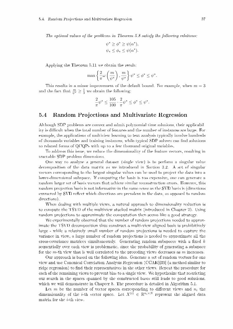
5.4. Random Projections and Multivariate Regression 37
The optimal values of the problems in Theorem 5.8 satisfy the following relations:
ψ∗ ≥ φ∗ ≥ ψ(α∗),
ψ∗ ≤ φ∗ ≤ ψ(α∗).
Applying the Theorem 5.11 we obtain the result:
max
{2
πω
(m
ψ∗
),m
ψ∗
}ψ∗ ≤ φ∗ ≤ ψ∗.
This results in a minor improvement of the default bound. For example, when m = 3and the fact that m
ψ∗ ≥ 13 we obtain the following:
2
πψ∗ ≤ 105
100· 2
πψ∗ ≤ φ∗ ≤ ψ∗.
5.4 Random Projections and Multivariate Regression
Although SDP problems are convex and admit polynomial time solutions, their applicabil-ity is di�cult when the total number of features and the number of instances are large. Forexample, the applications of multiview learning to text analysis typically involve hundredsof thousands variables and training instances, while typical SDP solvers can �nd solutionsto relaxed forms of QCQPs with up to a few thousand original variables.
To address this issue, we reduce the dimensionality of the feature vectors, resulting intractable SDP problem dimensions.
One way to analyze a general dataset (single view) is to perform a singular valuedecomposition of the data matrix as we introduced in Section 3.2. A set of singularvectors corresponding to the largest singular values can be used to project the data into alower-dimensional subspace. If computing the basis is too expensive, one can generate arandom larger set of basis vectors that achieve similar reconstruction errors. However, thisrandom projection basis is not informative in the same sense as the SVD basis is (directionsextracted by SVD re�ect which directions are prevalent in the data, as opposed to randomdirections).
When dealing with multiple views, a natural approach to dimensionality reduction isto compute the TSVD of the multiview stacked matrix (introduced in Chapter 2). Usingrandom projections to approximate the computation then seems like a good strategy.
We experimentally observed that the number of random projections needed to approx-imate the TSVD decomposition thus construct a multi-view aligned basis is prohibitivelylarge - while a relatively small number of random projections is needed to capture thevariance in view, a large number of random projections is needed to approximate all thecross-covariance matrices simultaneously. Generating random subspaces with a �xed ksequentially over each view is problematic, since the probability of generating a subspacefor the m-th view that is well correlated to the preceding views decreases as m increases.
Our approach is based on the following idea. Generate a set of random vectors for oneview and use Canonical Correlation Analysis Regression (CCAR)[33] (a method similar toridge regression) to �nd their representatives in the other views. Repeat the procedure foreach of the remaining views to prevent bias to a single view. We hypothesize that restrictingour search in the spaces spanned by the constructed bases still leads to good solutions,which we will demonstrate in Chapter 8. The procedure is detailed in Algorithm 5.1.
Let m be the number of vector spaces corresponding to di�erent views and ni thedimensionality of the i-th vector space. Let X(i) ∈ Rni×N represent the aligned datamatrix for the i-th view.
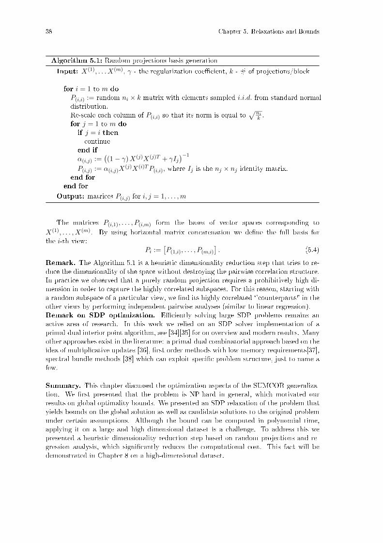
38 Chapter 5. Relaxations and Bounds
Algorithm 5.1: Random projections basis generation
Input: X(1), . . . X(m), γ - the regularization coe�cient, k - # of projections/block
for i = 1 to m doP(i,i) := random ni × k matrix with elements sampled i.i.d. from standard normaldistribution.Re-scale each column of P(i,i) so that its norm is equal to
√nik .
for j = 1 to m doif j = i thencontinue
end ifα(i,j) :=
((1− γ)X(j)X(j)T + γIj
)−1
P(i,j) := α(i,j)X(j)X(i)TP(i,i), where Ij is the nj × nj identity matrix.
end forend for
Output: matrices P(i,j) for i, j = 1, . . . ,m
The matrices P(i,1), . . . , P(i,m) form the bases of vector spaces corresponding toX(1), . . . , X(m). By using horizontal matrix concatenation we de�ne the full basis forthe i-th view:
Pi :=[P(1,i), . . . , P(m,i)
]. (5.4)
Remark. The Algorithm 5.1 is a heuristic dimensionality reduction step that tries to re-duce the dimensionality of the space without destroying the pairwise correlation structure.In practice we observed that a purely random projection requires a prohibitively high di-mension in order to capture the highly correlated subspaces. For this reason, starting witha random subspace of a particular view, we �nd its highly correlated `'counterparts" in theother views by performing independent pairwise analyses (similar to linear regression).Remark on SDP optimization. E�ciently solving large SDP problems remains anactive area of research. In this work we relied on an SDP solver implementation of aprimal-dual interior point algorithm, see [34][35] for on overview and modern results. Manyother approaches exist in the literature: a primal-dual combinatorial approach based on theidea of multiplicative updates [36], �rst-order methods with low memory requirements[37],spectral bundle methods [38] which can exploit speci�c problem structure, just to name afew.
Summary. This chapter discussed the optimization aspects of the SUMCOR generaliza-tion. We �rst presented that the problem is NP-hard in general, which motivated ourresults on global optimality bounds. We presented an SDP relaxation of the problem thatyields bounds on the global solution as well as candidate solutions to the original problemunder certain assumptions. Although the bound can be computed in polynomial time,applying it on a large and high dimensional dataset is a challenge. To address this wepresented a heuristic dimensionality reduction step based on random projections and re-gression analysis, which signi�cantly reduces the computational cost. This fact will bedemonstrated in Chapter 8 on a high-dimensional dataset.

39
Chapter 6
Cross-Lingual Document Similarity
Document similarity is an important component in techniques from text mining and naturallanguage processing. Many techniques use the similarity as a black box, e.g., a kernel inSupport Vector Machines. Comparison of documents (or other types of text snippets) in amonolingual setting is a well-studied problem in the �eld of information retrieval [39]. We�rst formally introduce the problem followed by a description of our novel approach.
6.1 Problem De�nition
We will �rst describe how documents are represented as vectors and how to comparedocuments in a mono-lingual setting. We then de�ne a way to measure cross-lingualsimilarity which is natural for the models we consider.Document Representation. The standard vector space model [39] represents documentsas vectors, where each term corresponds to a word or a phrase in a �xed vocabulary.Formally, document d is represented by a vector x ∈ Rn, where n corresponds to thesize of the vocabulary, and vector elements xk correspond to the number of times term koccurred in the document, also called term frequency or TFk(d).
For our document representation we applied a term re-weighting scheme that adjustsfor the fact that some words occur more frequently in general. A term weight should corre-spond to the importance of the term for the given corpus. The common weighting schemeis called Term Frequency Inverse Document Frequency (TFIDF ) weighting. An Inverse
Document Frequency (IDF ) weight for the dictionary term k is de�ned as log(
NDFk
),
where DFk is the number of documents in the corpus which contain term k and N is thetotal number of documents in the corpus. In the other part of our system, we computedTFIDF vectors on streams of news articles in multiple languages. There the IDF scoresfor each language changed dynamically - for each new document we computed the IDF ofall news articles within a ten day window.
The TFIDF weighted vector space model document representation corresponds to amap φ : text→ Rn de�ned by:
φ(d)k = TF k(d) log
(N
DF k
).
Monolingual similarity. A common way of computing similarity between documents iscosine similarity,
sim(d1, d2) =〈φ(d1), φ(d2)〉‖φ(d1)‖‖φ(d2)‖
,
where 〈·, ·〉 and ‖ · ‖ are standard inner product and Euclidean norm respectively. Whendealing with two or more languages, one could ignore the language information and build

40 Chapter 6. Cross-Lingual Document Similarity
a vector space using the union of tokens over the languages. A cosine similarity function insuch a space can be useful to some extent, for example �Internet� or �Bowie� may appearboth in Spanish and English texts and the presence of such terms in both an English and aSpanish document would contribute to their similarity. In general however, large parts ofvocabularies may not intersect. This means that given a language pair, many words in bothlanguages cannot contribute to the similarity score. Such cases can make the similarityfunction very insensitive to the data.Cross-Lingual Similarity. Processing a multilingual dataset results in several vectorspaces with varying dimensionality, one for each language. The dimensionality of thevector space corresponding to the i-th language is denoted by ni and the vector space modelmapping is denoted by φi : text → Rni . The similarity between documents in language iand language j is de�ned as a bilinear operator represented as a matrix Si,j ∈ Rni×nj :
simi,j(d1, d2) =〈φi(d1), Si,jφj(d2)〉‖φi(d1)‖‖φj(d2)‖
,
where d1 and d2 are documents written in the i-th and j-th language respectively. If themaximal singular value of Si,j is bounded by 1, then the similarity scores will lie on theinterval [−1, 1]. We will provide an overview of the models in Section 6.2, present relatedwork in Section 6.3 and then introduce additional notation in Section 6.4. Starting withSection 6.5 and ending with Section 6.8 we will describe some approaches to compute Si,jgiven training data.
6.2 Cross-Lingual Models
In this chapter we will describe several approaches to the problem of computing the mul-tilingual similarities introduced in Section 6.1. We present four approaches: a simpleapproach based on k-means clustering in Section 6.5, a standard approach based on sin-gular value decomposition in Section 6.6, a related approach called Canonical CorrelationAnalysis (CCA) in Section 6.7 and �nally a new method, which is an extension of CCA tomore than two languages in Section 6.8.
CCA can be used to �nd correlated patterns for a pair of languages, whereas theextended method optimizes a Sum of Squared Correlations (SSCOR) between several lan-guage pairs, which was introduced in [7]. The SSCOR problem is di�cult to solve in oursetting (hundreds of thousands of features, hundreds of thousands of examples). To tacklethis, we propose a method which consists of two ingredients. The �rst one is based on anobservation that certain datasets (such as Wikipedia) are biased towards one language (En-glish for Wikipedia), which can be exploited to reformulate a di�cult optimization problemas an eigenvector problem. The second ingredient is dimensionality reduction using CL-LSI, which makes the eigenvector problem computationally and numerically tractable.
We concentrate on approaches that are based on linear maps rather than alternatives,such as machine translation and probabilistic models, as discussed in the section on relatedwork. We will start by introducing some notation.
The thesis so far focused on the SUMCOR problem formulation, where two extensionswere proposed in Chapter 4 while Chapter 5 presented results on the problem complexityand global optimality bounds. In contrast, this chapter focuses on the SSCOR formulation.This is due to the fact that under an additional assumption (data is biased towards oneview), the problem simpli�es signi�cantly (we could not derive a similar result for SUM-COR). At the end of the chapter we will comment further on the SUMCOR formulationin light of the additional assumption which made SSCOR computationally tractable.

6.3. Related Work 41
6.3 Related Work
In this section, we describe previous work described in the literature. We have grouped theapproaches to cross-lingual similarity computation as those that are based on: translationand dictionaries, probabilistic topic models, matrix factorization, monolingual models andneural network word embeddings. We also present some related work that also uses theWikipedia as a language resource.
Translation and dictionary based. The most obvious way to compare documentswritten in di�erent languages is to use machine translation and perform monolingual sim-ilarity, see [40] and [41] for several variations of translation based approaches. One canuse free tools such as Moses [42] or translation services, such as Google Translate1. Thereare two issues with such approaches: they solve a harder problem than needs to be solvedand they are less robust to training resource quality - large sets of translated sentencesare typically needed. Training Moses for languages with scarce linguistic resources is thusproblematic. The issue with using online services such as Google Translate is that the APIsare limited and not free. The operation e�ciency and cost requirements make translation-based approaches less suited for our system. Closely related are works Cross-LingualVector Space Model (CL-VSM) [41] and the approach presented in [43] which both com-pare documents by using dictionaries, which in both cases are EuroVoc dictionaries [44].The generality of such approaches is limited by the quality of available linguistic resources,which may be scarce or non-existent for certain language pairs.
Probabilistic topic models. There exist many variants to modelling documentsin a language independent way by using probabilistic graphical models. The models in-clude: Joint Probabilistic Latent Semantic Analysis (JPLSA) [45], Coupled Probabilis-tic LSA (CPLSA) [45], Probabilistic Cross-Lingual LSA (PCLLSA) [46] and PolylingualTopic Models (PLTM) [47] which is a Bayesian version of PCLLSA. The methods (exceptfor CPLSA) describe the multilingual document collections as samples from generativeprobabilistic models, with variations on the assumptions on the model structure. Thetopics represent latent variables that are used to generate observed variables (words), aprocess speci�c to each language. The parameter estimation is posed as an inference prob-lem which is typically intractable and one usually solves it using approximate techniques.Most variants of solutions are based on Gibbs sampling or Variational Inference, whichare nontrivial to implement and may require an experienced practitioner to be applied.Furthermore, representing a new document as a mixture of topics is another potentiallyhard inference problem which must be solved.
Matrix factorization. Several matrix factorization based approaches exist in the lit-erature. The models include: Non-negative matrix factorization based [48], Cross-LingualLatent Semantic Indexing CL-LSI [49] and [40], Canonical Correlation Analysis (CCA) [1],Oriented Principal Component Analysis (OPCA) [45]. The quadratic time and space de-pendency of the OPCA method makes it impractical for large scale purposes. In addition,OPCA forces the vocabulary sizes for all languages to be the same, which is less intuitive.For our setting, the method in [48] has a prohibitively high computational cost whenbuilding models (it uses dense matrices whose dimensions are a product of the training setsize and the vocabulary size). Our proposed approach combines CCA and CL-LSI. An-other closely related method is Cross-Lingual Explicit Semantic Analysis (CL-ESA) [50],which uses Wikipedia (as do we in the current work) to compare documents. It can beinterpreted as using the sample covariance matrix between features of two languages tode�ne the dot product which is used to compute similarities. The authors of CL-ESAcompare it to CL-LSI and �nd that CL-LSI can outperform CL-ESA in an information
1https://translate.google.com/

42 Chapter 6. Cross-Lingual Document Similarity
retrieval, but is costlier to optimize over a large corpus (CL-ESA requires no training).We �nd that the scalability argument does not apply in our case: based on advances innumerical linear algebra we can solve large CL-LSI problems (millions of documents asopposed to the 10,000 document limit reported in [50][51]). In addition, CL-ESA is lesssuited for computing similarities between two large monolingual streams. For example,each day we have to compute similarities between 500,000 English and 500,000 Germannews articles. Comparing each German news article with 500,000 English news articles iseither prohibitively slow (involves projecting all English articles on Wikipedia) or consumestoo much memory (involves storing the projected English articles, which for a Wikipedia ofsize 1,000,000 is a 500,000 by 1,000,000 non-sparse matrix). An interesting combination ofdictionaries, CCA and LSI is presented in [52], where the authors show how to incorporatemultilingual evidence into independently built (monolingual) vector spaces. In [53] theauthors investigated how to optimally select an LSI training dataset for speci�c classi�-cation tasks and thus built domain speci�c common document representations, which isinteresting but less relevant to our problem setting.
Monolingual. Related work also includes monolingual approaches that treat docu-ment written in di�erent languages in a monolingual fashion. The intuition is that namedentities (for example, �Bowie�) and cognate words (for example, �tsunami�) are written inthe same or similar fashion in many languages. For example, the Cross-Language Char-acter n-Gram Model (CL-CNG) [41] represents documents as bags of character n-grams.Another approach is to use language dependent keyword lists based on cognate words[43]. These approaches may be suitable for comparing documents written in languagesthat share a writing system, which does not apply to the case of global news tracking.
Word embeddings and neural networks. Many approaches in the recent literaturefocus on neural network models which construct hierarchical (distributed) representationsof data. See [54],[55],[56] and [57] for an empirical comparison of several architectures over avariety of tasks. The approaches typically involve many tuning parameters (learning rates,batch sizes, neural network architectures) and the training tends to be computationallyintensive.
Wikipedia based. Finally, there are some works that use Wikipedia to build models,but are not necessarily focused on cross-lingual similarity learning. For example [58] useWikipedia for building cross-lingual dictionary that maps phrases from other languagesto English wikipedia concepts. Wikipedia was also used to build an entity matchingmodel [59], with the aim of aligning Wikipedia infoboxes. In [60] the authors investi-gated several cross-lingual measures between web documents (based on link analysis, aswell as the distribution of cognate words, character n-grams etc.) and found that it espe-cially valuable for under-resourced languages. Another paper [61] used Wikipedia conceptsas an inverted index to build cross-lingual similarities. The approach represented words asdistributions over Wikipedia concepts, which is closely related to [50].
6.4 Notation
The cross-lingual similarity models presented in this paper are based on comparable cor-pora. A comparable corpus is a collection of documents in multiple languages, with align-ment between documents that are of the same topic, or even a rough translation of eachother. Wikipedia is an example of a comparable corpus, where a speci�c entry can be de-scribed in multiple languages (e.g., �Berlin" is currently described in 222 languages). Newsarticles represent another example, where the same event can be described by newspapersin several languages.
More formally, a multilingual document d = (u1, . . . um) is a tuple of m documents

6.5. k-means 43
{{X
X1
X2
X3 {s
d1 d2 d3
{N{{
{
{
{{
{
n1
n2
n3
nm
ds
Xm X(:, 1)(m) X(:, 2)(m) X(:, 3)(m) X(:, s)(m)
X(:, s)(3)
X(:, s)(2)
X(:, s)(1)X(:, 3)(1)X(:, 2)(1)X(:, 1)(1)
X(:, 1)(2)
X(:, 1)(3) X(:, 2)(3) X(:, 3)(3)
X(:, 3)(2)X(:, 2)(2)
Figure 6.1: Multilingual corpora and their matrix representations using the vector spacemodel.
on the same topic (comparable), where ui is the document written in language i. Notethat an individual document ui can be an empty document (missing resource) and each dmust contain at least two nonempty documents. This means that in our analysis wediscard strictly monolingual documents for which no cross-lingual information is available.A comparable corpus D = d1, . . . , ds is a collection of s multilingual documents. By usingthe vector space model, we can represent D as a set of m multiview aligned matrices:X1, . . . , Xm, where Xi ∈ Rni×s is the matrix corresponding to the language i and ni is thevocabulary size of language i. Furthermore, let Xi(:, `) denote the `-th column of matrixXi and the matrices respect the document alignment - the vector Xi(:, `) corresponds tothe TFIDF vector of the i-th component of multilingual document d`. We use N to denotethe total row dimension of X, i.e., N :=
∑mi=1 ni. See Figure 6.1 for an illustration of the
introduced notation. The dimensions of each view form a block structure b := (b1, . . . , bm)and we will use the parenthesis notation x(i) to denote the i-th block according to thatblock structure.
We will now describe four models to cross-lingual similarity computation, where the�rst three are based on methods introduced in Chapter 3 and the fourth one represents anoriginal contribution.
6.5 k-means
We have introduced the k-means algorithm in Section 3.1 and we now discuss how to applyit to build a cross-lingual similarity function. In a nutshell, we apply the standard k-meansprocedure to the stacked multiview matrix and interpret the centroids as an aligned basis,which is used to build the CL-similarity model; see Figure 6.2 for an illustration of theapproach.
In order to apply the algorithm, we �rst merge all the term-document matrices into asingle matrix X by stacking the individual term-document matrices (as seen in Figure 6.1):
X :=[XT
1 , XT2 , · · · , XT
m
]T,
such that the columns respect the alignment of the documents (here MATLAB notationfor concatenating matrices is used). Therefore, each document is represented by a longvector indexed by the terms in all languages.
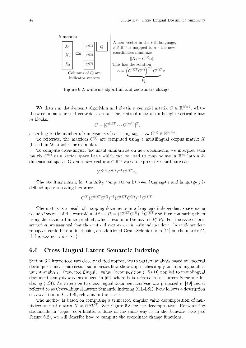
44 Chapter 6. Cross-Lingual Document Similarity
k-means:
⇠=This has the solution
X1
X2
X3
Q
Pi
{Columns of Q are
indicator vectors
C(1)
C(2)
C(3)
||Xi � C(i)�||
� =�C(i)T C(i)
��1C(i)T x
A new vector in the i-th language,x � Rni is mapped to � - the newcoordinates minimize
Figure 6.2: k-means algorithm and coordinate change.
We then run the k-means algorithm and obtain a centroid matrix C ∈ RN×k, wherethe k columns represent centroid vectors. The centroid matrix can be split vertically intom blocks:
C = [C(1)T · · ·C(mT )]T ,
according to the number of dimensions of each language, i.e., C(i) ∈ Rni×k.To reiterate, the matrices C(i) are computed using a multilingual corpus matrix X
(based on Wikipedia for example).To compute cross-lingual document similarities on new documents, we interpret each
matrix C(i) as a vector space basis which can be used to map points in Rni into a k-dimensional space. Given a new vector x ∈ Rni we can express its coordinates as:
(C(i)TC(i))−1C(i)Txi.
The resulting matrix for similarity computation between language i and language j isde�ned up to a scaling factor as:
C(i)(C(i)TC(i))−1(C(j)TC(j))−1C(j)T .
The matrix is a result of mapping documents in a language independent space usingpseudo-inverses of the centroid matrices Pi = (C(i)TC(i))−1C(i)T and then comparing themusing the standard inner product, which results in the matrix P Ti Pj . For the sake of pre-sentation, we assumed that the centroid vectors are linearly independent. (An independentsubspace could be obtained using an additional Gram-Schmidt step [11] on the matrix C,if this was not the case.)
6.6 Cross-Lingual Latent Semantic Indexing
Section 3.2 introduced two closely related approaches to pattern analysis based on spectraldecompositions. This section summarizes how these approaches apply to cross-lingual doc-ument analysis. Truncated Singular value Decomposition (TSVD) applied to monolingualdocument analysis was introduced in [62] where it is referred to as Latent Semantic In-dexing (LSI). An extension to cross-lingual document analysis was proposed in [49] and isreferred to as Cross-Lingual Latent Semantic Indexing (CL-LSI). Now follows a descriptionof a variation of CL-LSI, relevant to the thesis.
The method is based on computing a truncated singular value decomposition of mul-tiview stacked matrix X ≈ USV T . See Figure 6.3 for the decomposition. Representingdocuments in �topic� coordinates is done in the same way as in the k-means case (seeFigure 6.2), we will describe how to compute the coordinate change functions.
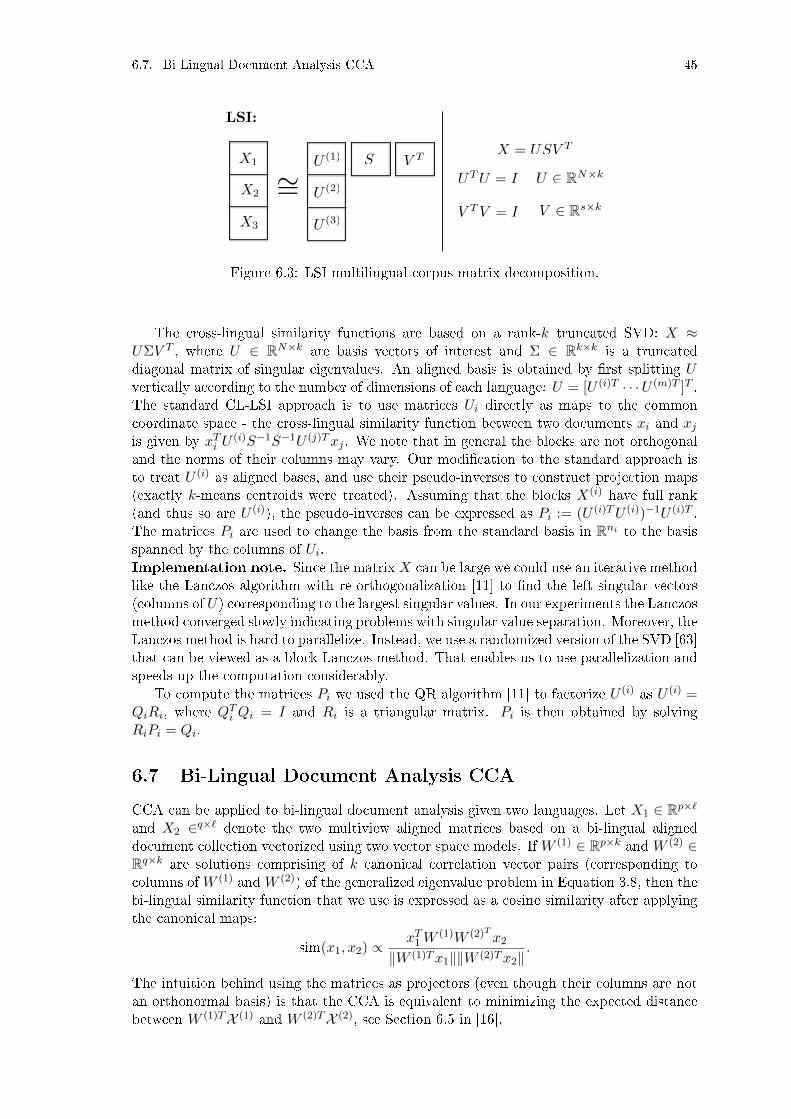
6.7. Bi-Lingual Document Analysis CCA 45
LSI:
⇠=X1
X2
X3
V T
V TV = I
UTU = I U 2 RN⇥k
V 2 Rs⇥k
X = USV T
SU (1)
U (2)
U (3)
Figure 6.3: LSI multilingual corpus matrix decomposition.
The cross-lingual similarity functions are based on a rank-k truncated SVD: X ≈UΣV T , where U ∈ RN×k are basis vectors of interest and Σ ∈ Rk×k is a truncateddiagonal matrix of singular eigenvalues. An aligned basis is obtained by �rst splitting Uvertically according to the number of dimensions of each language: U = [U (i)T · · ·U (m)T ]T .The standard CL-LSI approach is to use matrices Ui directly as maps to the commoncoordinate space - the cross-lingual similarity function between two documents xi and xjis given by xTi U
(i)S−1S−1U (j)Txj . We note that in general the blocks are not orthogonaland the norms of their columns may vary. Our modi�cation to the standard approach isto treat U (i) as aligned bases, and use their pseudo-inverses to construct projection maps(exactly k-means centroids were treated). Assuming that the blocks X(i) have full rank(and thus so are U (i)), the pseudo-inverses can be expressed as Pi := (U (i)TU (i))−1U (i)T .The matrices Pi are used to change the basis from the standard basis in Rni to the basisspanned by the columns of Ui.Implementation note. Since the matrix X can be large we could use an iterative methodlike the Lanczos algorithm with re-orthogonalization [11] to �nd the left singular vectors(columns of U) corresponding to the largest singular values. In our experiments the Lanczosmethod converged slowly indicating problems with singular value separation. Moreover, theLanczos method is hard to parallelize. Instead, we use a randomized version of the SVD [63]that can be viewed as a block Lanczos method. That enables us to use parallelization andspeeds up the computation considerably.
To compute the matrices Pi we used the QR algorithm [11] to factorize U (i) as U (i) =QiRi, where QTi Qi = I and Ri is a triangular matrix. Pi is then obtained by solvingRiPi = Qi.
6.7 Bi-Lingual Document Analysis CCA
CCA can be applied to bi-lingual document analysis given two languages. Let X1 ∈ Rp×`and X2 ∈q×` denote the two multiview aligned matrices based on a bi-lingual aligneddocument collection vectorized using two vector space models. If W (1) ∈ Rp×k and W (2) ∈Rq×k are solutions comprising of k canonical correlation vector pairs (corresponding tocolumns ofW (1) andW (2)) of the generalized eigenvalue problem in Equation 3.8, then thebi-lingual similarity function that we use is expressed as a cosine similarity after applyingthe canonical maps:
sim(x1, x2) ∝xT1W
(1)W (2)T x2
‖W (1)Tx1‖‖W (2)Tx2‖.
The intuition behind using the matrices as projectors (even though their columns are notan orthonormal basis) is that the CCA is equivalent to minimizing the expected distancebetween W (1)TX (1) and W (2)TX (2), see Section 6.5 in [16].

46 Chapter 6. Cross-Lingual Document Similarity
6.8 Hub Language Based CCA Extension
Building cross-lingual similarity models based on comparable corpora is challenging for twomain reasons. The �rst problem is related to missing alignment data: when a number oflanguages is large, the dataset of documents that cover all languages is small (or may evenbe empty). Even if only two languages are considered, the set of aligned documents canbe small (an extreme example is given by the Piedmontese and Hindi Wikipedias whereno inter-language links are available), in which case none of the methods presented so farare applicable.
The second challenge is scale - the data is high-dimensional (many languages withhundreds of thousands of features per language) and the number of multilingual docu-ments may be large (over one million in case of Wikipedia). The optimization problemposed by CCA is not trivial to solve: the covariance matrices themselves are prohibitivelylarge to �t in memory (even storing a 100,000 by 100,000 element matrix requires 80GBof memory) and iterative matrix-multiplication based approaches to solving generalizedeigenvalue problems are required (the covariance matrices can be expressed as products ofsparse matrices, which means we have fast matrix-vector multiplication).
We now describe an extension of CCA to more than two languages, which can be trainedon large comparable corpora and can handle missing data. The extension we consider isbased on a generalization of CCA to more than two views, introduced in [7], namely theSum of Squared Correlations SSCOR, introduced in Equation SSCOR in Section 4.2, whichwe will re-state formally later in this section. Our approach exploits a certain characteristicof the data, namely the hub language characteristic (see below) in two ways: to reducethe dimensionality of the data and to simplify the optimization problem. We focus onthe SSCOR formulation as opposed to the SCOR formulation which we explored in theprevious chapters, since the Lagrangian problem is easier to solve (That is under the hublanguage assumption, which we present next).Hub language characteristic. In the case of Wikipedia, we observed that even thoughthe training resources are scarce for certain language pairs, there often exists indirect train-ing data. By considering a third language, which has training data with both languagesin the pair, we can use the composition of learned maps as a proxy. We refer to this thirdlanguage as a hub language.
A hub language is a language with a high proportion of non-empty documents in D ={d1, ..., d`}. As we have mentioned, we only focus on multilingual documents that includeat least two languages. The prototypical example in the case of Wikipedia is English. Ournotion of the hub language could be interpreted in the following way. If a non-EnglishWikipedia page contains one or more links to variants of the page in other languages,English is very likely to be one of them. That makes English a hub language.
We use the following notation to de�ne subsets of the multilingual comparable corpus:let a(i, j) denote the index set of all multilingual documents with non-missing data for thei-th and j-th language:
a(i, j) = {k | dk = (u1, ..., um), ui 6= ∅, uj 6= ∅} ,
and let a(i) denote the index set of all multilingual documents with non missing data forthe i-th language.
We now describe a two step approach to building a cross-lingual similarity matrix. The�rst part is related to LSI and reduces the dimensionality of the data. The second stepre�nes the linear mappings and optimizes the linear dependence between data.Step 1: Hub language based dimensionality reduction. The �rst step in our methodis to project X1, . . . , Xm to lower-dimensional spaces without destroying the cross-lingual

6.8. Hub Language Based CCA Extension 47
structure. Treating the nonzero columns of Xi as observation vectors sampled from anunderlying distribution X (i) ∈ Rni , we can analyze the empirical cross-covariance matrices:
C(i,j) =1
|a(i, j)| − 1
∑
`∈a(i,j)
(Xi(:, `)− ci) · (Xj(:, `)− cj)T ,
where ci = 1|ai|∑
`∈a(i)Xi(:, `). By �nding low-rank approximations of C(i,j) we can identify
the subspaces that are relevant for extracting linear patterns between X (i) and X (j). LetX1
represent the hub language corpus matrix. The LSI approach to �nding the subspaces is toperform the singular value decomposition on the full N×N covariance matrix composed ofblocks C(i,j). If |a(i, j)| is small for many language pairs (as it is in the case of Wikipedia),then many empirical estimates C(i,j) are unreliable, which can result in over�tting. Forthis reason, we perform the truncated singular value decomposition on the matrix C =[C(1,2) · · ·C(1,m)] ≈ USV T , where U ∈ Rn1×k, S ∈ Rk×k, V ∈ R(
∑mi=2 ni)×k. De�ne T =
[UTV T ]T ∈ RN×k, which is compatible with the block structure b = (n1, . . . , nm). Notethat the columns of T (1) are orthonormal, but that is not true in general for the otherblocks. We proceed by reducing the dimensionality of each Xi by setting: Yi = T (i)T ·Xi,where Yi ∈ Rk×s. To summarize, the �rst step reduces the dimensionality of the data andis based on CL-LSI, but optimizes only the hub language related cross-covariance blocks.Step 2: Simplifying and solving SSCOR. The second step involves solving a gen-eralized version of canonical correlation analysis on the matrices Yi in order to �nd themappings Pi. The approach is based on the sum of squares of correlations formulationby Kettenring [7], where we consider only correlations between pairs (Y1, Yi), i > 1 dueto the hub language problem characteristic. We will present the original unconstrainedoptimization problem, then a constrained formulation based on the hub language problemcharacteristic. Then we will simplify the constraints and reformulate the problem as aneigenvalue problem by using Lagrange multipliers.
The original sum of squared correlations is formulated as an unconstrained problem:
maximizewi∈Rk
m∑
i<j
ρ(wTi Yi, wTj Yj)
2.
We solve a similar problem by restricting i = 1 and omitting the optimization over non-hub language pairs. Let Di,i ∈ Rk×k denote the empirical covariance of Yi and Di,j denotethe empirical cross-covariance computed based on Yi and Yj . We solve the followingconstrained (unit variance constraints) optimization problem:
maximizewi∈Rk
m∑
i=2
(wT1D1,iwi
)2subject to wTi Di,iwi = 1, ∀i = 1, . . . ,m. (6.1)
The constraints wTi Di,iwi can be simpli�ed by using the Cholesky decomposition Di,i =KTi · Ki and substitution: yi := Kiwi. By inverting the Ki matrices and de�ning Gi :=
K−T1 D1,iK−1i , the problem can be reformulated:
maximizeyi∈Rk
m∑
i=2
(yT1 Giyi
)2subject to yTi yi = 1, ∀i = 1, . . . ,m. (6.2)
A necessary condition for optimality is that the derivatives of the Lagrangian vanish. TheLagrangian of (6.2) is expressed as:
L(y1, . . . , ym, λ1, . . . , λm) =m∑
i=2
(yT1 Giyi
)2+
m∑
i=1
λi(yTi yi − 1
).
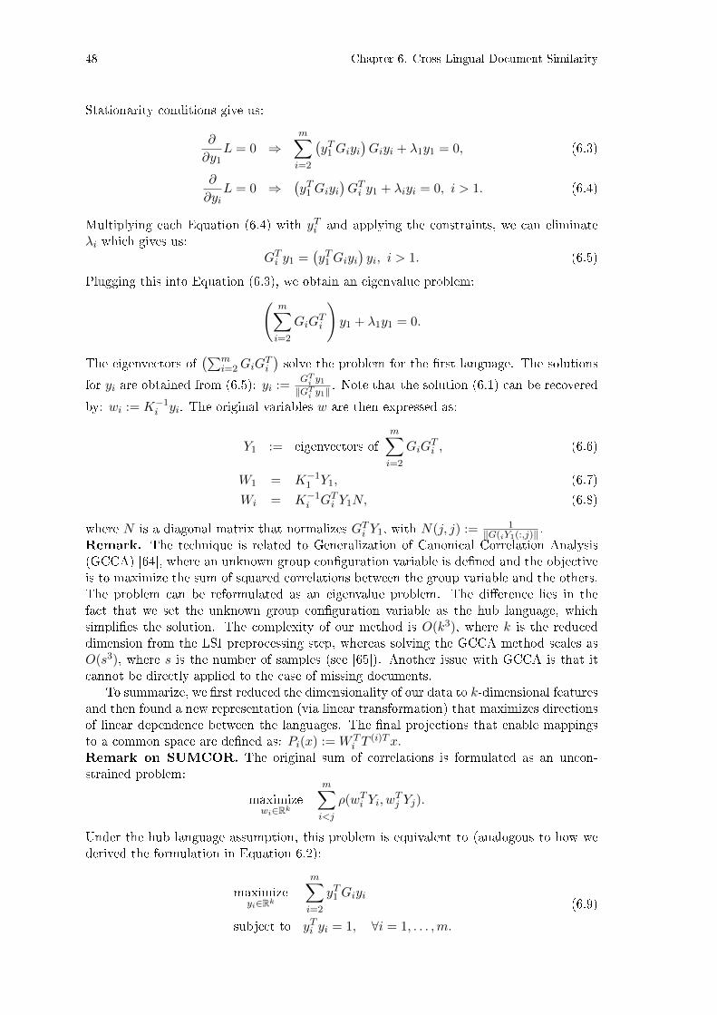
48 Chapter 6. Cross-Lingual Document Similarity
Stationarity conditions give us:
∂
∂y1L = 0 ⇒
m∑
i=2
(yT1 Giyi
)Giyi + λ1y1 = 0, (6.3)
∂
∂yiL = 0 ⇒
(yT1 Giyi
)GTi y1 + λiyi = 0, i > 1. (6.4)
Multiplying each Equation (6.4) with yTi and applying the constraints, we can eliminateλi which gives us:
GTi y1 =(yT1 Giyi
)yi, i > 1. (6.5)
Plugging this into Equation (6.3), we obtain an eigenvalue problem:(
m∑
i=2
GiGTi
)y1 + λ1y1 = 0.
The eigenvectors of(∑m
i=2GiGTi
)solve the problem for the �rst language. The solutions
for yi are obtained from (6.5): yi :=GT
i y1‖GT
i y1‖. Note that the solution (6.1) can be recovered
by: wi := K−1i yi. The original variables w are then expressed as:
Y1 := eigenvectors ofm∑
i=2
GiGTi , (6.6)
W1 = K−11 Y1, (6.7)
Wi = K−1i GTi Y1N, (6.8)
where N is a diagonal matrix that normalizes GTi Y1, with N(j, j) := 1‖G(iY1(:,j)‖ .
Remark. The technique is related to Generalization of Canonical Correlation Analysis(GCCA) [64], where an unknown group con�guration variable is de�ned and the objectiveis to maximize the sum of squared correlations between the group variable and the others.The problem can be reformulated as an eigenvalue problem. The di�erence lies in thefact that we set the unknown group con�guration variable as the hub language, whichsimpli�es the solution. The complexity of our method is O(k3), where k is the reduceddimension from the LSI preprocessing step, whereas solving the GCCA method scales asO(s3), where s is the number of samples (see [65]). Another issue with GCCA is that itcannot be directly applied to the case of missing documents.
To summarize, we �rst reduced the dimensionality of our data to k-dimensional featuresand then found a new representation (via linear transformation) that maximizes directionsof linear dependence between the languages. The �nal projections that enable mappingsto a common space are de�ned as: Pi(x) := W T
i T(i)Tx.
Remark on SUMCOR. The original sum of correlations is formulated as an uncon-strained problem:
maximizewi∈Rk
m∑
i<j
ρ(wTi Yi, wTj Yj).
Under the hub language assumption, this problem is equivalent to (analogous to how wederived the formulation in Equation 6.2):
maximizeyi∈Rk
m∑
i=2
yT1 Giyi
subject to yTi yi = 1, ∀i = 1, . . . ,m.
(6.9)

6.8. Hub Language Based CCA Extension 49
The Lagrangian of (6.9) is expressed as:
L(y1, . . . , ym, λ1, . . . , λm) =m∑
i=2
yT1 Giyi +m∑
i=1
λi(yTi yi − 1
).
Stationarity conditions give us:
∂
∂y1L = 0 ⇒
m∑
i=2
Giyi + λ1y1 = 0,
∂
∂yiL = 0 ⇒ GTi y1 + λiyi = 0, i > 1.
(6.10)
It follows that:Giyi = − 1
λiGiG
Ti y1,
and thus:m∑
i=2
− 1
λiGiG
Ti y1 + λ1y1 = 0.
Since the following equality can be derived:
λ1 =m∑
i=2
λi
the original problem reduces to
m∑
i=2
− 1
λiGiG
Ti y1 +
m∑
i=2
λiy1 = 0,
but the solution to that problem does not seem obvious. This is in contrast to the SSCORproblem, where all λi as well as yi could be eliminated simultaneously.
Summary. This chapter presented the problem of computing cross-lingual documentsimilarities and then presented four computational approaches to solve the problem. Thelast one is an original contribution of the author. It is based on combining an e�cientpreprocessing step with a particular generalization of CCA (SSCOR), which under anadditional assumption (hub language) can be solved e�ciently (both the preprocessingstep as well as the simplifying assumption are crucial for the approach). The next chapterwill discuss an application of cross-lingual similarity learning to a large scale cross-lingualnews analysis system.


51
Chapter 7
Applications to Cluster Linking
In online media streams � particularly news articles � there is often duplication of report-ing, di�erent viewpoints or opinions, all centering around a single event. Typically eachevent is covered by many articles and the question we address is how to �nd all the articlesin di�erent languages that are reporting on the same event. The current chapter describesan application of the cross-lingual similarity presented in Chapter 6 to cross-lingual clusterlinking. The application is relevant for monitoring global news in multiple languages. Pre-sented in the current chapter is our original approach to cross-lingual cluster linking, whichwas published in [9]. The main idea in our approach is to combine semantic informationextraction with cross-lingual document analysis, which we proved to be e�ective in [10].There we used a simpler set of features to decide which clusters to link and put greateremphasis on the manual evaluation of the quality.
To prepare the ground for the discussion of the cross-lingual approach, we will �rstdescribe how events are de�ned for our purposes and sketch a general approach to eventtracking in a monolingual setting.
The term event is vague and ambiguous, but for the practical purposes, we de�ne itas �any signi�cant happening that is being reported about in the media�. Examples ofevents would include shooting down of the Malaysia Airlines plane over Ukraine on July18th, 2014 (see Figure 7.1) and HSBC's admittance of aiding their clients in tax evasionon February 9th, 2015. Events such as these are covered by many articles and the questionis how to �nd all the articles in di�erent languages that are describing a single event.Generally, events are more speci�c than general themes as the time component plays animportant role � for example, the two wars in Iraq would be considered as separate events.
We take a pragmatic approach where the events are identi�ed as the clusters discov-ered by stream clustering algorithm that is designed to cluster news articles together iftheir content is similar and they are published close in time.
The particular choice of a streaming clustering algorithm is not relevant to the discus-sion of our approach and we assume that given a monolingual news stream, we have at ourdisposal an online clustering component which assigns to each news article a cluster ID. Inthis work we used the clustering component of the Event Registry [66] and [67] system.
We now consider the case where we are dealing with several document streams, whereeach stream corresponds to a particular language. Running the monolingual streamingclustering on each stream results in clusters within streams that need to be matched acrossstreams, which we will state formally.

52 Chapter 7. Applications to Cluster Linking
Figure 7.1: Events are represented by collections of articles about an event, in this casethe Malaysian Airlines plane which was shot down over Ukraine. The results shown inthe �gure can be obtained using the query http://eventregistry.org/event/997350#
?lang=eng&tab=articles. The content presented is part of the Event Registry system.
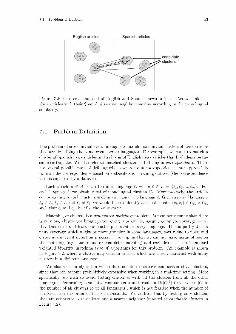
7.1. Problem De�nition 53
English articles Spanish articles
candidate clusters
Figure 7.2: Clusters composed of English and Spanish news articles. Arrows link En-glish articles with their Spanish k-nearest neighbor matches according to the cross-lingualsimilarity.
7.1 Problem De�nition
The problem of cross-lingual event linking is to match monolingual clusters of news articlesthat are describing the same event across languages. For example, we want to match acluster of Spanish news articles and a cluster of English news articles that both describe thesame earthquake. We also refer to matched clusters as to being in correspondence. Thereare several possible ways of de�ning when events are in correspondence - our approach isto learn the correspondence based on a classi�cation training dataset (the correspondenceis thus captured by a dataset).
Each article a ∈ A is written in a language `, where ` ∈ L = {`1, `2, ..., `m}. Foreach language `, we obtain a set of monolingual clusters C`. More precisely, the articlescorresponding to each cluster c ∈ C` are written in the language `. Given a pair of languages`a ∈ L, `b ∈ L and `a 6= `b, we would like to identify all cluster pairs (ci, cj) ∈ C`a × C`bsuch that ci and cj describe the same event.
Matching of clusters is a generalized matching problem. We cannot assume that thereis only one cluster per language per event, nor can we assume complete coverage � i.e.,that there exists at least one cluster per event in every language. This is partly due tonews coverage which might be more granular in some languages, partly due to noise anderrors in the event detection process. This implies that we cannot make assumptions onthe matching (e.g., one-to-one or complete matching) and excludes the use of standardweighted bipartite matching type of algorithms for this problem. An example is shownin Figure 7.2, where a cluster may contain articles which are closely matched with manyclusters in a di�erent language.
We also seek an algorithm which does not do exhaustive comparison of all clusters,since that can become prohibitively expensive when working in a real-time setting. Morespeci�cally, we wish to avoid testing cluster ci with all the clusters from all the otherlanguages. Performing exhaustive comparison would result in O(|C|2) tests, where |C| isthe number of all clusters (over all languages), which is not feasible when the number ofclusters is on the order of tens of thousands. We address this by testing only clustersthat are connected with at least one k-nearest neighbor (marked as candidate clusters inFigure 7.2).
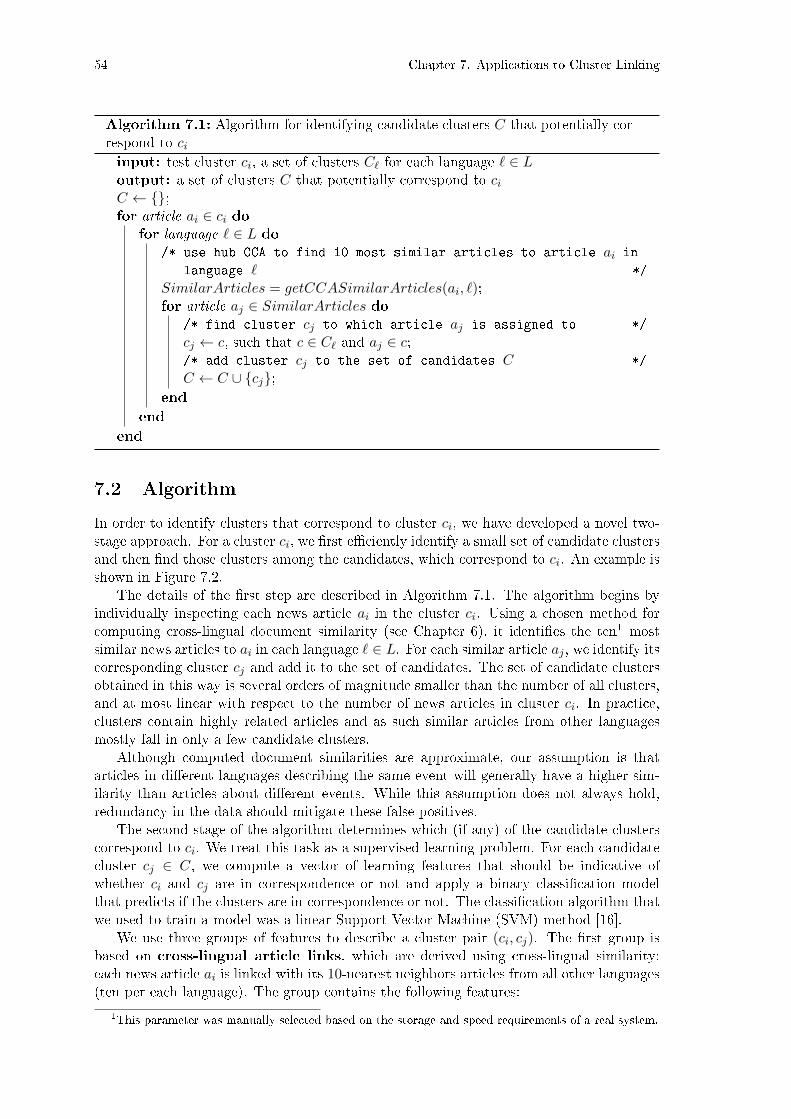
54 Chapter 7. Applications to Cluster Linking
Algorithm 7.1: Algorithm for identifying candidate clusters C that potentially cor-respond to ciinput: test cluster ci, a set of clusters C` for each language ` ∈ Loutput: a set of clusters C that potentially correspond to ciC ← {};for article ai ∈ ci do
for language ` ∈ L do/* use hub CCA to find 10 most similar articles to article ai in
language ` */
SimilarArticles = getCCASimilarArticles(ai, `);for article aj ∈ SimilarArticles do
/* find cluster cj to which article aj is assigned to */
cj ← c, such that c ∈ C` and aj ∈ c;/* add cluster cj to the set of candidates C */
C ← C ∪ {cj};end
end
end
7.2 Algorithm
In order to identify clusters that correspond to cluster ci, we have developed a novel two-stage approach. For a cluster ci, we �rst e�ciently identify a small set of candidate clustersand then �nd those clusters among the candidates, which correspond to ci. An example isshown in Figure 7.2.
The details of the �rst step are described in Algorithm 7.1. The algorithm begins byindividually inspecting each news article ai in the cluster ci. Using a chosen method forcomputing cross-lingual document similarity (see Chapter 6), it identi�es the ten1 mostsimilar news articles to ai in each language ` ∈ L. For each similar article aj , we identify itscorresponding cluster cj and add it to the set of candidates. The set of candidate clustersobtained in this way is several orders of magnitude smaller than the number of all clusters,and at most linear with respect to the number of news articles in cluster ci. In practice,clusters contain highly related articles and as such similar articles from other languagesmostly fall in only a few candidate clusters.
Although computed document similarities are approximate, our assumption is thatarticles in di�erent languages describing the same event will generally have a higher sim-ilarity than articles about di�erent events. While this assumption does not always hold,redundancy in the data should mitigate these false positives.
The second stage of the algorithm determines which (if any) of the candidate clusterscorrespond to ci. We treat this task as a supervised learning problem. For each candidatecluster cj ∈ C, we compute a vector of learning features that should be indicative ofwhether ci and cj are in correspondence or not and apply a binary classi�cation modelthat predicts if the clusters are in correspondence or not. The classi�cation algorithm thatwe used to train a model was a linear Support Vector Machine (SVM) method [16].
We use three groups of features to describe a cluster pair (ci, cj). The �rst group isbased on cross-lingual article links, which are derived using cross-lingual similarity:each news article ai is linked with its 10-nearest neighbors articles from all other languages(ten per each language). The group contains the following features:
1This parameter was manually selected based on the storage and speed requirements of a real system.

7.2. Algorithm 55
• linkCount is the number of times any of the news articles from cj is among 10-nearest neighbors for articles from ci. In other words, it is the number of times anarticle from ci has a very similar article (i.e., is among 10 most similar) in cj .
• avgSimScore is the average similarity score of the links, as identi�ed for linkCount,between the two clusters.
Remark. The size of the nearest neighbor sets in our experiments is set to 10. The pa-rameter was manually set with the goal of keeping computational and storage requirementslow, while still capturing the cross-lingual correspondences.
The second group are concept-related features. Articles that are imported intoEvent Registry are annotated by disambiguating mentioned entities and keywords to thecorresponding Wikipedia pages [68]. Whenever �David Bowie� is, for example, mentionedin the article, the article is annotated with a link to his Wikipedia page. In the sameway, all mentions of entities (people, locations, organizations) and ordinary keywords (e.g.,�bank�, �tax�, �ebola�, �plane�, �company�) are annotated. Although the Spanish articleabout �Bowie� will be annotated with his Spanish version of the Wikipedia page, in manycases we can link the Wikipedia pages to their English versions. This can be done sinceWikipedia itself provides information regarding which pages in di�erent languages representthe same concept/entity. Using this approach, the word �avión� in a Spanish article willbe annotated with the same concept as the word �plane� in an English article. Althoughthe articles are in di�erent languages, the annotations can therefore provide a language-independent vocabulary that can be used to compare articles/clusters. By analyzing allthe articles in clusters ci and cj , we can identify the most relevant entities and keywordsfor each cluster. Additionally, we can also assign weights to the concepts based on howfrequently they occur in the articles in the cluster. From the list of relevant concepts andcorresponding weights, we consider the following features:
• entityCosSim is the cosine similarity between vectors of entities from clusters ci andcj .
• keywordCosSim is the cosine similarity between vectors of keywords from clusters ciand cj .
• entityJaccardSim is Jaccard similarity coe�cient [69] between sets of entities fromclusters ci and cj .
• keywordJaccardSim is Jaccard similarity coe�cient between sets of keywords fromclusters ci and cj .
The last group of features contains three miscellaneous features that seem discrim-inative but are unrelated to the previous two groups:
• hasSameLocation feature is a boolean variable that is true when the location of theevent in both clusters is the same. The location of events is estimated by consideringthe locations mentioned in the articles that form a cluster and is provided by EventRegistry.
• timeDiff is the absolute di�erence in hours between the two events. The publicationtime and date of the events is computed as the average publication time and date ofall the articles and is provided by Event Registry.

56 Chapter 7. Applications to Cluster Linking
• sharedDates is determined as the Jaccard similarity coe�cient between sets of datementions extracted from articles. We use extracted mentions of dates provided byEvent Registry, which uses an extensive set of regular expressions to detect andnormalize mentions of dates in di�erent forms.
Summary. This chapter presented an application of the cross-lingual models on the taskof linking news clusters across several languages. The approach is based on formulatingthe problem as a classi�cation problem and using several sets of features, most notably:cross-lingual similarity based and semantic extraction (concepts-related) based features.In Chapter 8 we will presents some experiments and investigate the applicability of theproposed approach.

57
Chapter 8
Experiments
This chapter presents several experiments that explore how the theory relates to practice.The �rst set of experiments focuses on global optimality and convergence rates on syntheticdata. We then move to cross-lingual document analysis and examine the performance ofour approach on the task of information retrieval based on training sets with missing data.Finally we evaluate our approach to cross-lingual cluster linking.
8.1 Synthetic Experiments
We generated several multiview problem instances by varying the number of views andnumber of dimensions per view in order to compare the performance of local search methodsand the proposed SDP relaxation. The goal of these experiments was to see under whichconditions and how often do the global bounds provide useful information. The mainobservations are that the set of problems where the bounds are useful has a non-zeromeasure and that the di�culty of the optimization problem increases with the number ofviews and decreases with the number of dimensions per view.
8.1.1 Generating Synthetic Problem Instances
Let m denote the number of views (sets of variables) and ni denote the dimensionality ofi-th view and N :=
∑i ni. In all cases, we used the same number of dimensions per view
(n1 = n2 = · · · = nm). We used three di�erent methods to generate random correlationmatrices.
The �rst method, the random Gram matrix method (see [70], [71]), generates thecorrelation matrices by sampling N vectors v1, . . . , vn for an N -dimensional multivariateGaussian distribution (centered at the origin, with an identity covariance matrix), normal-izing them and computing the correlation matrix C = [ci,j ]N×N as ci,j := vTi · vj .
The second method, the random spectrum method, samples the eigenvaluesλ1, . . . , λN uniformly from a simplex (
∑Ni=1 λi = N) and generates a random correlation
matrix with the prescribed eigenvalues (see [71]).The �nal method, the random 1-dim structure method, generates a correlation
matrix that has an approximately (due to noise) single-dimensional correlation structure.We generate a random m dimensional Gram matrix B, and insert it into an N × Nidentity matrix according to the block structure to obtain a matrix C0. That is, we setC0 (i, j) = δ (i, j), where δ is the Kronecker delta. For I, J = 1 . . . ,m, we override theentries
C0
(1 +
I−1∑
i=1
ni, 1 +J−1∑
i=1
ni
)= B (I, J) ,
58 Chapter 8. Experiments
where we used 1-based indexing. We then generate a random Gram matrix D ∈ RN×Nand compute the �nal correlation matrix as C = (1− ε)C0 + εD. In our experiments, weset ε = 0.001.
The purpose of using a random spectrum method is that as the dimensionality increases,random vectors tend to be orthogonal, hence the experiments based on random Grammatrices might be less informative. As the experiments show, the local method su�ers whenall ni = 1 (an instance of a BQO problem). By using the approximately 1-dimensionalcorrelation matrix sampling, we investigated how the problem behaves when ni > 1.
In all cases, we perform a �nal step that involves computing the per-view Choleskydecompositions of variances and change of basis (as in QCQP).
8.1.2 Convergence of Horst's algorithm on Synthetic Data
We �rst present an empirical inquiry of the convergence rate of the Horst's algorithm.In Figure 8.1, we generated 1, 000 random instances of matrices A with block structureb = (2, 2, 2, 2, 2), where we used the random Gram matrix method. For each matrix, wegenerated a starting point x0 and ran the algorithm. The plot depicts the solution changerate on a logarithmic scale (log10
‖xold−x‖‖x‖ ). We observe linear convergence over a wide range
of rates of convergence (slopes of the lines). Figure 8.2 shows the convergence propertiesfor a �xed matrix A with several random initial vectors x0. The problem exhibits a globaland a local solution. For 65% of the initial vectors, the global solution was reached (versus35% for the local solution). Note that the global solution paths tend to converge faster(the average global solution path slope is −0.08, compared to −0.05 for the local solutionpaths).
8.1.3 SDP and Horst Solutions on Synthetic Problems
We also explored how the number of views and the dimensionality of the problems relatesto the di�culty of �nding globally optimal solutions, for all aforementioned methods ofgenerating random problem instances. For each sampling scenario and each choice of mand ni, we generated 100 experiments, and computed 1, 000 solutions based on Algorithm4.1, the SDP solution (and respective global bounds), and examined the frequencies of thefollowing events:
• a relaxation gap candidate detected (Tables 8.1, 8.2, 8.3 (a))
• local convergence detected (Tables 8.1, 8.2, 8.3 (b))
• when a local solution is worse than the SDP-based lower bound (Tables 8.1, 8.2,8.3 (c)).
The possibility of a relaxation gap is detected when the best local solution is lower than1% of the SDP bound. In this case, the event indicates only the possibility of relaxationgap � it might be the case that further local algorithm restarts would close the gap. Localconvergence is detected when the objective value of two local solutions di�ers relatively byat least 10% and absolutely at least by 0.1 (both criteria must be satis�ed simultaneously).Finally, the event of a local solution being below the SDP lower bound means that it isbelow 2
π of the optimal objective value of the SDP relaxation.We �nd that regardless of the generation technique, the lower SDP bound is useful
only when ni = 1 (Table 8.1, 8.2, 8.3 (c)) and the results are similar for di�erent choicesof m. There are, however, rare instances (less than 0.1%) where the lower bound is usefulfor ni = 2 and even rarer (less than 0.01%) for ni = 3.

8.1. Synthetic Experiments 59
0 50 100 150−18
−16
−14
−12
−10
−8
−6
−4
−2
0
2
iteration number
log10norm(x
old−x)
norm(x
)
5−th percentile
25−th percentile
50−th percentile
75−th percentile
95−th percentile
sample paths
Figure 8.1: Convergence plot (1, 000 random matrices A, one random x0 per probleminstance).
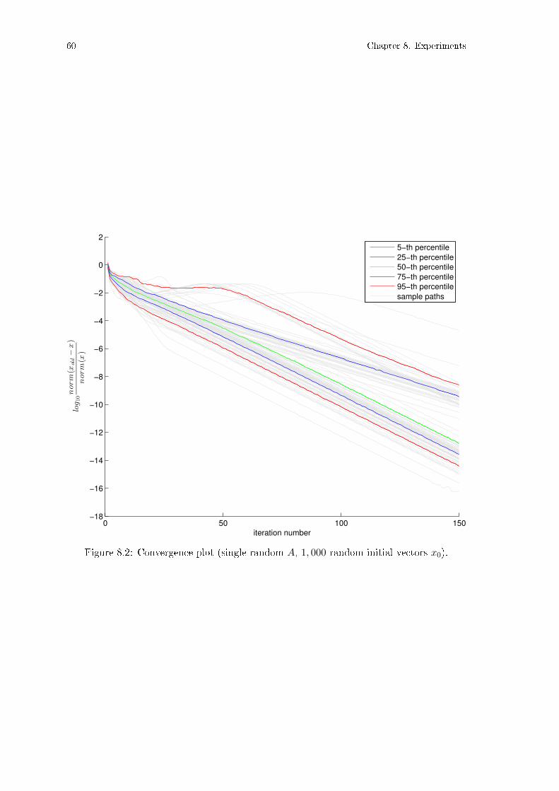
60 Chapter 8. Experiments
0 50 100 150−18
−16
−14
−12
−10
−8
−6
−4
−2
0
2
iteration number
log10norm(x
old−x)
norm(x
)
5−th percentile
25−th percentile
50−th percentile
75−th percentile
95−th percentile
sample paths
Figure 8.2: Convergence plot (single random A, 1, 000 random initial vectors x0).

8.2. Experiments on EuroParl Corpus 61
Table 8.1: Random Gram matrix.
(a) Possible relaxation gap.
ni = 3 ni = 2 ni = 1
m = 5 0% 5% 17%m = 3 0% 0% 9%
(b) Local convergence.
ni = 3 ni = 2 ni = 1
m = 5 1% 5% 48%m = 3 0% 1% 26%
(c) Local solution below lower SDP bound.
ni = 3 ni = 2 ni = 1
m = 5 0% 0% 14%m = 3 0% 0% 12%
Table 8.2: Random spectrum sampling.
(a) Possible relaxation gap.
ni = 3 ni = 2 ni = 1
m = 5 0% 5% 36%m = 3 0% 1% 20%
(b) Local convergence.
ni = 3 ni = 2 ni = 1
m = 5 1% 3% 50%m = 3 0% 0% 31%
(c) Local solution below lower SDP bound.
ni = 3 ni = 2 ni = 1
m = 5 0% 0% 15%m = 3 0% 0% 16%
The chance of local convergence increases as the number of views m increases whichcan be consistently observed for all choices of ni and sampling strategies. Generating ageneric problem where the local algorithm converges to a local solution is less likely as thedimensionality increases (Tables 8.1, 8.2).
In the case of noisy embeddings of a 1-dimensional correlation structures, the de-pendence on ni behaves di�erently: the local convergence (see Table 8.3b) for the case(m = 5, ni = 3) is more likely than for the case (m = 5, ni = 2). This is unexpected as inthe general case, increasing ni reduces that chance of local convergence, see Table 8.2b,Table 8.1b.
The relationship between m and ni and the possibility of a relaxation gap behavessimilarly as local convergence - increasing m increases it and increasing ni decreases it(Table 8.1a, Table 8.2a), except in the case of noisy 1-dim correlation structures, where weobserve the same anomaly when ni = 2 (Table 8.3a).
Therefore we have demonstrated that there exist sets of problems with nonzero measurewhere the SDP bounds give useful information.
8.2 Experiments on EuroParl Corpus
Applications of canonical correlation analysis on collections of documents include: di-mensionality reduction, cross-lingual document retrieval and classi�cation [18] and [72],multilingual topic extraction [73] and news bias detection [74]. In this section, we explorethe behavior of Algorithm 4.1 with respect to the global bounds on real data, computed
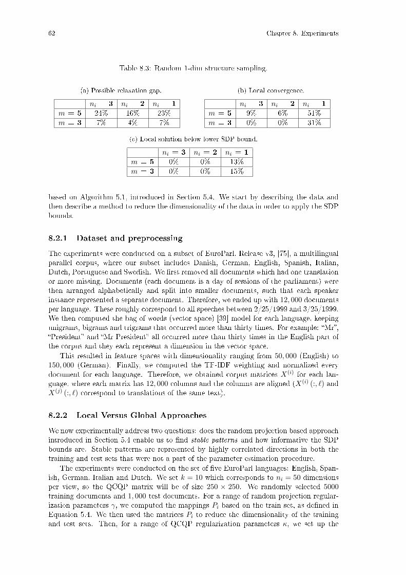
62 Chapter 8. Experiments
Table 8.3: Random 1-dim structure sampling.
(a) Possible relaxation gap.
ni = 3 ni = 2 ni = 1
m = 5 24% 16% 23%m = 3 7% 4% 7%
(b) Local convergence.
ni = 3 ni = 2 ni = 1
m = 5 9% 6% 51%m = 3 0% 0% 31%
(c) Local solution below lower SDP bound.
ni = 3 ni = 2 ni = 1
m = 5 0% 0% 13%m = 3 0% 0% 15%
based on Algorithm 5.1, introduced in Section 5.4. We start by describing the data andthen describe a method to reduce the dimensionality of the data in order to apply the SDPbounds.
8.2.1 Dataset and preprocessing
The experiments were conducted on a subset of EuroParl, Release v3, [75], a multilingualparallel corpus, where our subset includes Danish, German, English, Spanish, Italian,Dutch, Portuguese and Swedish. We �rst removed all documents which had one translationor more missing. Documents (each document is a day of sessions of the parliament) werethen arranged alphabetically and split into smaller documents, such that each speakerinstance represented a separate document. Therefore, we ended up with 12, 000 documentsper language. These roughly correspond to all speeches between 2/25/1999 and 3/25/1999.We then computed the bag of words (vector space) [39] model for each language, keepingunigrams, bigrams and trigrams that occurred more than thirty times. For example: �Mr�,�President� and �Mr President� all occurred more than thirty times in the English part ofthe corpus and they each represent a dimension in the vector space.
This resulted in feature spaces with dimensionality ranging from 50, 000 (English) to150, 000 (German). Finally, we computed the TF-IDF weighting and normalized everydocument for each language. Therefore, we obtained corpus matrices X(i) for each lan-guage, where each matrix has 12, 000 columns and the columns are aligned (X(i) (:, `) andX(j) (:, `) correspond to translations of the same text).
8.2.2 Local Versus Global Approaches
We now experimentally address two questions: does the random projection based approachintroduced in Section 5.4 enable us to �nd stable patterns and how informative the SDPbounds are. Stable patterns are represented by highly correlated directions in both thetraining and test sets that were not a part of the parameter estimation procedure.
The experiments were conducted on the set of �ve EuroParl languages: English, Span-ish, German, Italian and Dutch. We set k = 10 which corresponds to ni = 50 dimensionsper view, so the QCQP matrix will be of size 250 × 250. We randomly selected 5000training documents and 1, 000 test documents. For a range of random projection regular-ization parameters γ, we computed the mappings Pi based on the train set, as de�ned inEquation 5.4. We then used the matrices Pi to reduce the dimensionality of the trainingand test sets. Then, for a range of QCQP regularization parameters κ, we set up the

8.3. Experiments on the Wikipedia Corpus 63
Table 8.4: Train and test sum of correlation.
(a) Train set sum of correlations.
γ =0.1 γ =0.5 γ =0.9 γ =0.99
κ =0.01 10.0 9.8 9.8 9.8κ =0.1 10.0 9.8 9.8 9.8κ =0.5 10.0 9.8 9.8 9.8κ =0.9 10.0 9.8 9.8 9.8κ =0.99 10.0 9.8 9.7 9.8
(b) Test set sum of correlations.
γ =0.1 γ =0.5 γ =0.9 γ =0.99
κ =0.01 5.8 8.6 9.6 9.8κ =0.1 6.2 8.6 9.6 9.8κ =0.5 7.0 8.6 9.6 9.8κ =0.9 7.4 8.8 9.6 9.8κ =0.99 7.4 8.8 9.6 9.8
QCQP problem, computed 1, 000 local solutions (by Horst algorithm) and solved the SDPrelaxation. The whole procedure was repeated 10 times.
For each (γ, κ) pair, we measured the sum of correlations on the test and train sets.Table 8.4 shows the sums of correlations averaged over 10 experimental trials. The maximalpossible sum of correlations for �ve datasets is
(52
)= 10. We observed that regularizing
the whole optimization problem is not as vital as regularizing the construction of randomprojection vectors. This is intuitive, since �nding the random projection vectors involves aregression in a high dimensional space, a harder estimation problem as opposed to solvinga lower dimensional QCQP. The choice of γ = 0.1 lead to perfectly correlated solutionson the training set for all κ values. This turned out to be over-�tted when we evaluatedthe sum of correlations on the test set. Perfect correlations on the training set were notreproduced on the test set (the sum of correlations ranges between 5.8 and 7.4). Note thathigher κ values improved the performance on the test set up to a certain level below 7.5.As we increased γ to 0.5, we saw a reduction in over�tting and with γ = 0.9 stable patternswere observed.
We conclude that using appropriate regularization parameters, we can reduce the di-mensionality of the original QCQP problem and still �nd stable solutions.
The reduced dimensionality of the problem then enabled an investigation of the behav-ior of the SDP relaxation. For the SDP bounds, we observed behavior that was similar tothe high-dimensional synthetic (generic) case. That is we found that the potential relax-ation gap was very small and that the SDP and the Horst's algorithm yielded the sameresult. For this reason we omit the SDP results from Table 8.4.
8.3 Experiments on the Wikipedia Corpus
We will describe the main dataset for building cross-lingual models, which is based onWikipedia, and then present two sets of experiments. The �rst set of experiments estab-lishes that the hub based approach can deal with language pairs where little or no trainingdata is available. The second set of experiments compares the main approaches that we
64 Chapter 8. Experiments
presented on the task of mate retrieval and the task of event linking. In the mate retrievaltask we are given a test set of document pairs, where each pair consists of a documentand its translation. Given a query document from the test set, the goal is to retrieve itstranslation in the other language, which is also referred to as its mate document. Finally,we examine how di�erent choices of features impact the event linking performance.
8.3.1 Wikipedia Comparable Corpus
The following experiments are based on a large-scale real-world multilingual dataset ex-tracted from Wikipedia by using inter-language links for alignment. Wikipedia is a largesource of multilingual data that is especially important for the languages for which notranslation tools, multilingual dictionaries (e.g. Eurovoc [44]), or strongly aligned multi-lingual corpora (e.g. Europarl [75]) are available. Documents in di�erent languages arerelated with so-called inter-language links that can be found on the left of the Wikipediapage. The Wikipedia is constantly growing. At the time of writing the thesis there weretwelve Wikipedias with more than one million articles, 52 with more than one hundredthousand articles, 129 with more than ten thousand articles, and 236 with more than onethousand articles.
We now present some details on how the dataset was processed to obtain the cross-lingual aligned corpus. Each Wikipedia page is embedded in the page tag. First, weignored all the pages whose titles started with a Wikipedia namespace (which includescategories and discussion pages) and all redirection pages (but we stored the redirect linkbecause inter-language links can point to redirection links also). We removed the markupof all the pages that we processed.
We constructed the inter-language link matrix using the previously stored redirectionlinks and inter-language links. Inter-language links that pointed to the redirection linkswere replaced with the redirection target links. Since linking is not enforced to be consis-tent, we obtained a matrixM that was not symmetric. The existence of the inter-languagelink in one way (i.e., English to German) does not guarantee that there is an inter-languagelink in the reverse direction (German to English). To correct this we symmetrized the ma-trix M by computing M + MT and thus obtained an undirected graph. In the rare casethat after symmetrization we had multiple links pointing from a document, we kept the�rst link. Our experiments were based on Wikipedia dumps available in 2013.
8.3.2 Experiments With Missing Alignment Data
In this subsection, we will present the empirical performance of hub CCA approach. Wewill demonstrate that this approach can be successfully applied even in the case of fullymissing alignment information. To this purpose, we selected a subset of Wikipedia lan-guages containing three major languages, English (4,212k articles)�en (hub language),Spanish (9,686k articles)�es, Russian (9,662k articles)�ru, and �ve minority (in terms ofWikipedia sizes) languages, Slovenian (136k articles)�sl, Piedmontese (59k articles)�pms,Waray-Waray (112k articles)�war (all with about 2 million native speakers), Creole (54karticles)�ht (8 million native speakers), and Hindi (97k articles)�hi (180 million nativespeakers). For preprocessing, we removed the documents that contained less than 20 dif-ferent words (which are referred to as stubs1) and removed words that occurred in lessthan 50 documents as well as the top 100 most frequent words (in each language sepa-rately). We represented the documents as normalized TFIDF [39] weighted vectors. The
1Such documents are typically of low value as a linguistic resource. Examples include the titles of thecolumns in the table, remains of the parsing process, or Wikipedia articles with very little or no informationcontained in one or two sentences.
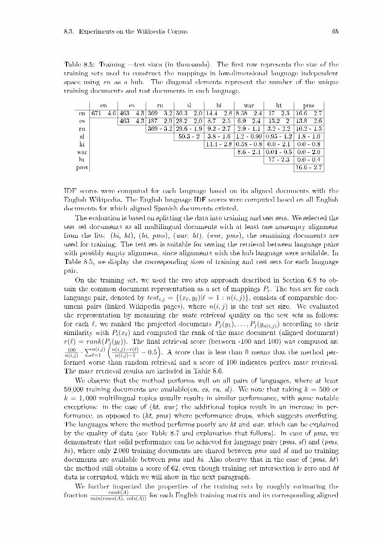
8.3. Experiments on the Wikipedia Corpus 65
Table 8.5: Training � test sizes (in thousands). The �rst row represents the size of thetraining sets used to construct the mappings in low-dimensional language independentspace using en as a hub. The diagonal elements represent the number of the uniquetraining documents and test documents in each language.
en es ru sl hi war ht pmsen 671 - 4.6 463 - 4.3 369 - 3.2 50.3 - 2.0 14.4 - 2.8 8.58 - 2.4 17 - 2.3 16.6 - 2.7es 463 - 4.3 187 - 2.9 28.2 - 2.0 8.7 - 2.5 6.9 - 2.4 13.2 - 2 13.8 - 2.6ru 369 - 3.2 29.6 - 1.9 9.2 - 2.7 2.9 - 1.1 3.2 - 2.2 10.2 - 1.3sl 50.3 - 2 3.8 - 1.6 1.2 - 0.99 0.95 - 1.2 1.8 - 1.0hi 14.4 - 2.8 0.58 - 0.8 0.0 - 2.1 0.0 - 0.8war 8.6 - 2.4 0.04 - 0.5 0.0 - 2.0ht 17 - 2.3 0.0 - 0.4pms 16.6 - 2.7
IDF scores were computed for each language based on its aligned documents with theEnglish Wikipedia. The English language IDF scores were computed based on all Englishdocuments for which aligned Spanish documents existed.
The evaluation is based on splitting the data into training and test sets. We selected thetest set documents as all multilingual documents with at least one nonempty alignmentfrom the list: (hi, ht), (hi, pms), (war, ht), (war, pms), the remaining documents areused for training. The test set is suitable for testing the retrieval between language pairswith possibly empty alignment, since alignments with the hub language were available. InTable 8.5, we display the corresponding sizes of training and test sets for each languagepair.
On the training set, we used the two step approach described in Section 6.8 to ob-tain the common document representation as a set of mappings Pi. The test set for eachlanguage pair, denoted by testi,j = {(x`, y`)|` = 1 : n(i, j)}, consists of comparable doc-ument pairs (linked Wikipedia pages), where n(i, j) is the test set size. We evaluatedthe representation by measuring the mate retrieval quality on the test sets as follows:for each `, we ranked the projected documents Pj(y1), . . . , Pj(yn(i,j)) according to theirsimilarity with Pi(x`) and computed the rank of the mate document (aligned document)r(`) = rank(Pj(y`)). The �nal retrieval score (between -100 and 100) was computed as:100n(i,j) ·
∑n(i,j)`=1
(n(i,j)−r(`)n(i,j)−1 − 0.5
). A score that is less than 0 means that the method per-
formed worse than random retrieval and a score of 100 indicates perfect mate retrieval.The mate retrieval results are included in Table 8.6.
We observe that the method performs well on all pairs of languages, where at least50,000 training documents are available(en, es, ru, sl). We note that taking k = 500 ork = 1, 000 multilingual topics usually results in similar performance, with some notableexceptions: in the case of (ht, war) the additional topics result in an increase in per-formance, as opposed to (ht, pms) where performance drops, which suggests over�tting.The languages where the method performs poorly are ht and war, which can be explainedby the quality of data (see Table 8.7 and explanation that follows). In case of pms, wedemonstrate that solid performance can be achieved for language pairs (pms, sl) and (pms,hi), where only 2,000 training documents are shared between pms and sl and no trainingdocuments are available between pms and hi. Also observe that in the case of (pms, ht)the method still obtains a score of 62, even though training set intersection is zero and ht
data is corrupted, which we will show in the next paragraph.We further inspected the properties of the training sets by roughly estimating the
fraction rank(A)min(rows(A), cols(A)) for each English training matrix and its corresponding aligned

66 Chapter 8. Experiments
Table 8.6: Pairwise retrieval, 500 topics on the left � 1,000 topics on the right.
en es ru sl hi war ht pmsen 98 - 98 95 - 97 97 - 98 82 - 84 76 - 74 53 - 55 96 - 97es 97 - 98 94 - 96 97 - 98 85 - 84 76 - 77 56 - 57 96 - 96ru 96 - 97 94 - 95 97 - 97 81 - 82 73 - 74 55 - 56 96 - 96sl 96 - 97 95 - 95 95 - 95 91 - 91 68 - 68 59 - 69 93 - 93hi 81 - 82 82 - 81 80 - 80 91 - 91 68 - 67 50 - 55 87 - 86war 68 - 63 71 - 68 72 - 71 68 - 68 66 - 62 28 - 48 24 - 21ht 52 - 58 63 - 66 66 - 62 61 - 71 44 - 55 16 - 50 62 - 49pms 95 - 96 96 - 96 94 - 94 93 - 93 85 - 85 23 - 26 66 - 54
Table 8.7: Dimensionality drift. Each column corresponds to a pair of aligned corpusmatrices between English and another language. The numbers represent the ratio betweenthe numerical rank and the highest possible rank. For example, the column en � ht tells usthat for the English-Creole pairwise-aligned corpus matrix pair, the English counterparthas full rank, but the Creole counterpart is far having full rank.
en � es en � ru en � sl en � hi en � war en � ht en � pms0.81 � 0.89 0.8 � 0.89 0.98 � 0.96 1 � 1 0.74 � 0.56 1 � 0.22 0.89 � 0.38
matrix of the other language, where rows(A) and cols(A) denote the number of rows andcolumns respectively. The denominator represents the theoretically highest possible rankthe matrix A could have. Ideally, these two fractions should be approximately the same- both aligned spaces should have reasonably similar dimensionality. We display thesenumbers as pairs in Table 8.7.
It is clear that in the case of the Creole language only at most 22% documents areunique and suitable for the training. Though we removed the stub documents, manyof the remaining documents are nearly indistinguishable, as the quality of some smallerWikipedias is low. This was con�rmed for the Creole, Waray-Waray, and Piedmonteselanguages by manual inspection. The low quality documents correspond to templatesabout the year, person, town, etc. and contain very few unique words.
There is also a problem with the quality of the test data. For example, if we look atthe test pair (war, ht) only 386/534 Waray-Waray test documents are unique but on theother side almost all Creole test documents (523/534) are unique. This indicates a pooralignment which leads to poor performance.
8.3.3 Evaluation Of Cross-Lingual Event Linking
We now turn our attention to the task of cross-lingual event linking and the evaluationof the novel approach presented in Chapter 7. In order to determine how accuratelywe can predict cluster correspondence, we performed two experiments in a multilingualsetting using English, German and Spanish languages for which we had labelled data toevaluate the linking performance. In the �rst experiment, we tested how well the individualapproaches for cross-lingual article linking perform when used for linking the clusters aboutthe same event. In the second experiment we tested how accurate the prediction model iswhen trained on di�erent subsets of learning features. To evaluate the prediction accuracy

8.3. Experiments on the Wikipedia Corpus 67
for a given dataset we used 10-fold cross validation.We created a manually labelled dataset in order to evaluate cross-lingual event linking
using two human annotators. The annotators were provided with an interface listing thearticles, their content from and top concepts for a pair of clusters and their task was todetermine if the clusters were in correspondence or not (i.e., discuss same event). Toobtain a pair of clusters (ci, cj) to annotate, we �rst randomly chose a cluster ci, usedAlgorithm 7.1 to compute a set of potentially corresponding clusters C and randomly chosea cluster cj ∈ C. The dataset provided by the annotators contains 808 examples, of which402 are cluster pairs in correspondence and 406 are not. Clusters in each learning exampleare either in English, Spanish or German. Although Event Registry imports articles inother languages as well, we restricted our experiments to these three languages. We choseonly these three languages since they have a very large number of articles and clusters perday which makes the cluster linking problem hard due to large number of possible links.
In Chapter 3 and Chapter 6, we described the three main algorithms for identifyingsimilar articles in di�erent languages. These algorithms were k-means, LSI and hub CCA.As a training set, we used common Wikipedia alignment for all three languages. To testwhich of these algorithms performed best, we made the following test. For each of thethree algorithms, we analyzed all articles in Event Registry and for each article computedthe most similar articles in other languages. To test how informative the identi�ed similararticles are for cluster linking we then trained three classi�ers as described in Section 7.2� one for each algorithm. Each classi�er was allowed to use as learning features onlythe cross-lingual article linking features for which values are determined based on theselected algorithm (k-means, LSI and hub CCA). The results of the trained models areshown in Table 8.8. We also show how the number of topics (the dimensions of the latentspace) in�uences the quality, except in the case of the k-means algorithm, where only theperformance on 500 topic vectors is reported, due to higher computational cost.
We observe that, for the task of cluster linking, LSI and hub CCA perform comparablyand both outperform k-means.
We also compared the proposed approaches on the task of Wikipedia mate retrieval(the same task as in Section 8.3.2). In our evaluation we used a measure referred to as theAverage Mean Reciprocal Rank (AMRR) [76]. Given a collection of Q queries q1, . . . , qQand their corresponding mate documents m1, . . . ,mQ, the Mean Reciprocal Rank (MRR)is expressed as:
MRR =1
Q
Q∑
i=1
1
rank(i),
where rank(i) refers to the rank position of the mate document mi with respect to thei-th query qi. The rank is obtained by sorting the similarity scores {sim(qi, rj)}Qj=1 indescending order. Since we are dealing with more than two languages, we averaged theMRR scores over several language pairs and this aggregate score is referred to as AMRR.
We computed the AMRR performance of the di�erent approaches on the Wikipediadata by holding out 15, 000 aligned test documents and using 300, 000 aligned documentsas the training set.
Figure 8.3 shows AMRR score as the function of the number of feature vectors. It isclear that hub CCA outperforms LSI approach and k-means lags far behind when testingon Wikipedia data. The hub CCA approach with 500 topic vectors manages to performcomparably to the LSI-based approach with 1, 000 topic vectors, which shows that theCCA method can improve both model memory footprint as well as similarity computationtime.
Furthermore, we inspected how the number of topics in�uences the accuracy of clusterlinking. As we can see from Table 8.8 choosing a number of features larger than 500
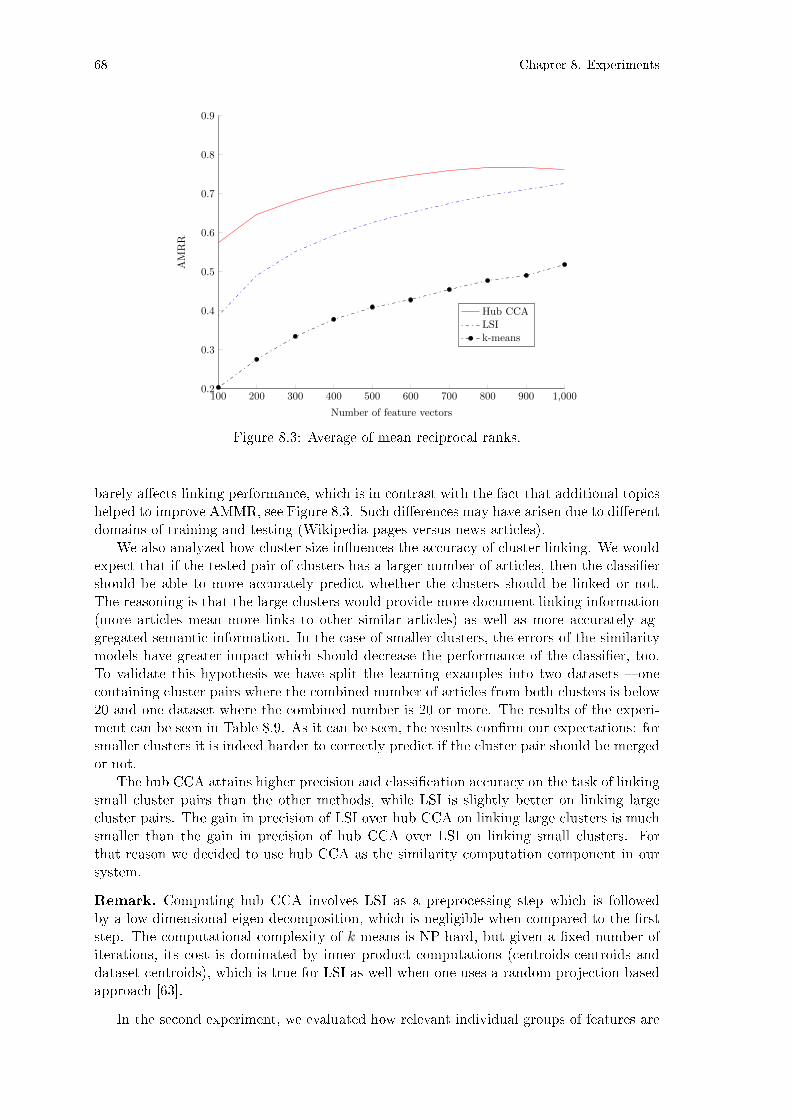
68 Chapter 8. Experiments
100 200 300 400 500 600 700 800 900 1,0000.2
0.3
0.4
0.5
0.6
0.7
0.8
0.9
Number of feature vectors
AMRR
Hub CCALSIk-means
Figure 8.3: Average of mean reciprocal ranks.
barely a�ects linking performance, which is in contrast with the fact that additional topicshelped to improve AMMR, see Figure 8.3. Such di�erences may have arisen due to di�erentdomains of training and testing (Wikipedia pages versus news articles).
We also analyzed how cluster size in�uences the accuracy of cluster linking. We wouldexpect that if the tested pair of clusters has a larger number of articles, then the classi�ershould be able to more accurately predict whether the clusters should be linked or not.The reasoning is that the large clusters would provide more document linking information(more articles mean more links to other similar articles) as well as more accurately ag-gregated semantic information. In the case of smaller clusters, the errors of the similaritymodels have greater impact which should decrease the performance of the classi�er, too.To validate this hypothesis we have split the learning examples into two datasets � onecontaining cluster pairs where the combined number of articles from both clusters is below20 and one dataset where the combined number is 20 or more. The results of the experi-ment can be seen in Table 8.9. As it can be seen, the results con�rm our expectations: forsmaller clusters it is indeed harder to correctly predict if the cluster pair should be mergedor not.
The hub CCA attains higher precision and classi�cation accuracy on the task of linkingsmall cluster pairs than the other methods, while LSI is slightly better on linking largecluster pairs. The gain in precision of LSI over hub CCA on linking large clusters is muchsmaller than the gain in precision of hub CCA over LSI on linking small clusters. Forthat reason we decided to use hub CCA as the similarity computation component in oursystem.
Remark. Computing hub CCA involves LSI as a preprocessing step which is followedby a low-dimensional eigen-decomposition, which is negligible when compared to the �rststep. The computational complexity of k-means is NP-hard, but given a �xed number ofiterations, its cost is dominated by inner product computations (centroids-centroids anddataset-centroids), which is true for LSI as well when one uses a random-projection basedapproach [63].
In the second experiment, we evaluated how relevant individual groups of features are

8.3. Experiments on the Wikipedia Corpus 69
Table 8.8: Accuracy of cluster linking with 500/800/1,000 topic vectors obtained fromdi�erent cross-lingual similarity algorithms. The table shows for each of the algorithmsthe obtained classi�cation accuracy, precision and recall. Some results related to k-meansare omitted, since the computation took too long and the algorithm's performance wasconsistently lower than the other methods considered.
Models Accuracy % Precision % Recall % F1 %hub CCA 78.2/79.6/80.3 76.3/78.0/80.5 81.6/82.1/79.9 78.9/80.0/80.2
LSI 78.9/78.7/80.6 76.8/77.0/78.7 83.3/80.6/83.6 79.9/78.8/81.1k-means 73.9/-/- 69.5/-/- 84.6/-/- 76.3/-/-
Table 8.9: Accuracy of cluster linking using 500 topic vectors on two datasets containinglarge (left number) and small (right number) clusters. The dataset with small clusterscontained the subset of learning examples in which the combined number of articles fromboth clusters of the cluster pair were below 20. The remaining learning examples were putinto the dataset of large clusters.
Models Accuracy % Precision % Recall % F1 %hub CCA 81.2 - 77.8 80.5 - 74.5 91.3 - 57.5 85.6 - 64.9
LSI 82.8 - 76.4 81.3 - 70.9 93.1 - 57.5 86.8 - 63.5k-means 75.5 - 71.2 72.8 - 70.8 95.3 - 36.2 82.5 - 47.9
to correctly determine cluster correspondence. For this purpose, we computed accuracyusing individual groups of features, as well as using di�erent combinations of groups. Sincehub CCA had the best performance of the three algorithms, we used it to compute thevalues of the cross-lingual article linking features. The results of the evaluation are shownin Table 8.10. We can see that using a single group of features, the highest predictionaccuracy can be achieved using concept-related features. The classi�cation accuracy inthis case is 88.5%. By additionally including also the cross-lingual article linking features,the classi�cation accuracy rises slightly to 89.4%. Using all three groups of features, theachieved accuracy is 89.2%.
To test if the accuracy of the predictions is language dependent we have also performedthe evaluations separately on individual language pairs. For this experiment we have splitthe annotated learning examples into three datasets, where each dataset contained onlyexamples for one language pair. When training the classi�er all three groups of featureswere available. The results are shown in Table 8.11. We can see that the performance ofcluster linking on the English-German dataset is the highest in terms of accuracy, preci-sion, recall and F1. The performance on the English-Spanish dataset is comparable to theperformance on the English-German dataset, where the former achieves higher recall (andslightly higher F1 score), while the latter achieves higher precision. A possible explana-tion of these results is that the higher quantity and quality of English-German languageresources leads to a more accurate cross-lingual article similarity measure as well as to amore extensive semantic annotation of the articles.
Based on the performed experiments, we can make the following conclusions. Thecross-lingual similarity algorithms provide valuable information that can be used to iden-

70 Chapter 8. Experiments
Table 8.10: The accuracy of the classi�er for story linking using di�erent sets of learningfeatures. See Section 7.2 for a description of di�erent feature sets that were used in classi�-cation: Concepts for concept-related features, Misc for miscellaneous features and HubCCA for features based cross-lingual article links using hub CCA.
Features Accuracy % Precision % Recall % F1 %Hub CCA 78.3± 5.9 78.2± 7.0 78.9± 5.2 78.4± 5.5Concepts 88.5± 2.7 88.6± 4.8 88.6± 2.2 88.5± 2.4Misc 54.8± 6.7 61.8± 16.5 58.2± 30.2 52.4± 13.0
Hub CCA + Concepts 89.4± 2.5 89.4± 4.6 89.6± 2.4 89.4± 2.3Hub CCA + Misc 78.8± 5.0 78.9± 7.1 79.4± 4.6 79.0± 4.5Concepts + Misc 88.7± 2.6 88.8± 4.6 88.8± 2.2 88.7± 2.3
All 89.2± 2.6 88.8± 4.9 90.1± 1.9 89.3± 2.3
Table 8.11: The accuracy of the classi�er for story linking on training data for each languagepair separately using all learning features.
Language pair Accuracy % Precision % Recall % F1 %en, de 91.8± 5.5 91.7± 6.3 93.7± 6.3 92.5± 5.1en, es 87.7± 5.4 87.7± 7.4 88.5± 9.8 87.6± 5.9es, de 88.6± 4.3 89.7± 9.1 84.3± 11.9 85.9± 6.0
tify clusters that describe the same event in di�erent languages. For the task of clusterlinking, the cross-lingual article linking features are however signi�cantly less informativecompared to the concept-related features that are extracted from the semantic annota-tions. Nevertheless, the cross-lingual article similarity features are very important for tworeasons. The �rst is that they allow us to identify for a given cluster a limited set ofcandidate clusters that are potentially in correspondence. This is a very important featuresince it reduces the search space by several orders of magnitude. The second reason thesefeatures are important is that concept annotations are not available for all articles as theannotation of news articles is computationally intensive and can only be done for a subsetof collected articles. The prediction accuracies for individual language pairs are compara-ble although it seems that the achievable accuracy correlates with the amount of availablelanguage resources.
8.3.4 Remarks on the Scalability of the Implementation
One of the main advantages of our two step approach to cross-lingual cluster linking isthat it is highly scalable. It is fast, very robust to the quality of training data, easilyextendable, simple to implement and has relatively small hardware requirements. Thesimilarity pipeline is the most computationally intensive part and currently runs on amachine with two Intel Xeon E5-2667 v2, 3.30GHz processors with 256GB of RAM. Thisis su�cient to do similarity computation over a large number of languages if needed. Itcurrently uses Wikipedia as a freely available knowledge base and experiments show thatthe similarity pipeline dramatically reduces the search space when linking clusters.
Currently, we compute similarities over 24 languages with tags: eng, spa, deu, zho, ita,
8.3. Experiments on the Wikipedia Corpus 71
fra, rus, swe, nld, tur, jpn, por, ara, �n, ron, kor, hrv, tam, hun, slv, pol, srp, cat, ukrbut we support any language from the top 100 Wikipedia languages. Our data streamscome from the service called Newsfeed (http://newsfeed.ijs.si/) which provides 430kunique articles per day. Our system currently computes 2 million similarities per second,that means that we compute 16 · 1010 similarities per day. We store one day bu�er foreach language which requires 1.5 GB of memory with documents stored as 500-dimensionalvectors. We note that the time complexity of the similarity computations scales linearlywith dimension of the feature space and does not depend on the number of languages. Foreach article, we compute the top 10 most similar ones in every other language.
For all linear algebra matrix and vector operations, we use high performance numericallinear algebra libraries as BLAS, OPENBLAS and Intel MKL, which currently allows usto process more than one million articles per day. In our current implementation, we usethe variation of the hub approach. Our projector matrices are of size 500 × 300, 000, soevery projector takes about 1.1 GB of RAM. Moreover, we need proxy matrices of size500 × 500 for every language pair. That is 0.5 GB for 24 languages and 9.2 GB for 100languages. Altogether we need around 135 GB of RAM for the system with 100 languages.Usage of proxy matrices enables the projection of all input documents in the commonspace and handling language pairs with missing or low alignment. That enables us todo block-wise similarity computations further improving system e�ciency. Our code cantherefore be easily parallelized using matrix multiplication rather than performing morematrix - vector multiplications. This speeds up our code roughly by a factor of 4. In thisway, we obtain some caching gains and ability to use vectorization. Our system is alsoeasily extendable. Adding a new language requires the computation of a projector matrixand proxy matrices with all other already available languages.
8.3.5 Remarks on the Reproducibility of Experiments
We have made both the code and data that were used in the experiments publicly availableat https://github.com/rupnikj/jair_paper.git. The manually labelled dataset usedin the evaluation of event linking is available at in the �dataset� subfolder of the githubrepository. The included archive contains two folders: �positive� and �negative�, wherethe �rst folder includes examples of cluster pairs in two languages that represent the sameevent and the second folder contains pairs of clusters in two languages that do not representdi�erent events. Each example is a JSON �le that contains at the top level informationabout a pair of clusters (including text of the articles) as well as a set of �meta� attributes,that correspond to features described in Section 7.2.
The �code� folder includes MATLAB scripts for building cross-lingual similarity modelsintroduced in Chapter 6, which can be used with publicly available Wikipedia corpusto reproduce the cross-lingual similarity evaluation. We have also made available thesimilarity computation over 100 languages as a service at xling.ijs.si.
In addition, the Event Registry system (http://eventregistry.org/) comes with anAPI, documented at https://github.com/gregorleban/event-registry-python, thatcan be used to download events and articles.

73
Chapter 9
Conclusions
9.1 Discussion
In the thesis we study a generalization of CCA to more than two sets of variables. Wepresent a new result that proves that the complexity of the SUMCOR problem is NP-hard and describe a novel approach to �nding several sets of nonlinear patterns,based on a locally convergent method. Experimentally, we observed that the performanceof the local method (with linear convergence) is generally good, although we identi�edproblem settings where convergence to local optima occurs (based on synthetic experi-ments we observed, that increasing the number of views increases the likelihood of suchevents). We present a novel SDP relaxation of the problem, which can be used to obtainnew local solutions and to provide several new computationally tractable bounds onglobal optimality of the SUMCOR problem solutions. The usefulness of the bounds is ex-plored on synthetic problem instances and problems related to cross-lingual text-mining.We introduce a new preprocessing step based on random projections to reducethe dimensionality of high dimensional problems such as in document corpora, makingmemory requirements tractable. We demonstrate the applicability of the approach onhigh-dimensional text data.
We present an application of two generalizations of CCA, the SUMCOR and SSCORformulations to cross-lingual similarity function learning. The cross-lingual similarityfunctions are applied to the task of cross-lingual cluster linking, where we present andevaluate a novel approach that combines features based on semantic and language analysis.The approach is shown to be scalable both in terms of number of articles and number oflanguages, while accurately linking events. The approach is used in a system for real-timemonitoring of global news in multiple languages, where a strong server is used to computetwo millions of similarities per second.
On the task of mate retrieval, we observe that re�ning the LSI-based projections withhub CCA leads to improved retrieval precision (hub CCA achieves 0.7 AMRR, whereasLSI achieves 0.6, when 500 dimensions are used), but the methods perform comparably onthe task of event linking (see Table 8.8). Further inspection showed that the CCA-basedapproach reached a higher precision on smaller clusters. The interpretation is that thelinking features are highly aggregated for large clusters, which compensates the lower per-document precision of LSI. Another possible reason is that the advantage that we show onWikipedia is lost on the news domain. This hypothesis could be validated by testing theapproach on documents from a di�erent domain.
The experiments show that the hub CCA-based features present a good baseline, whichcan greatly bene�t from additional semantic-based features (an increase in F1 score from0.78 to 0.88, see Table 8.10). Even though in our experiments the addition of CCA-based

74 Chapter 9. Conclusions
features to semantic features did not lead to great performance improvements (marginalincrease in performance when compared to concept based features, see Table 8.10), thereare two important bene�ts in the approach. First, the linking process can be sped upby using a smaller set of candidate clusters. Second, the approach is robust to languageswhere semantic extraction is not available, due to scarce linguistic resources. For examplein Tables 8.5 and 8.6 we demonstrate that similarity models based on our SSCOR refor-mulation under the hub language assumption can be built for language pairs withscarce and low quality linguistic resources. For example, the 0.85 retrieval score for thePiedmontese-Hindi pair reported in Table 8.6 is promising, since their bilingual trainingset was empty.
9.2 Future Work
Regarding the work on the SUMCOR formulation, the experiments indicate that the noisy1-dimensional embeddings present di�culties for the Horst's algorithm, which is in contrastto the performance on random generic problem instances. A natural question is, are thereother problem structures that result in suboptimal behavior of the local approach?
Our empirical results focus on text data, and an interesting direction is to extend theanalysis to data from other modalities, such as images, sensor streams and graphs.
Also of interest is the complexity analysis of the other generalizations proposed in [7].Regarding the work on cluster linking, the proposed cross-lingual analysis approaches
represent an important building block in our approach to cross-lingual cluster linking.The language component is built independently from the cluster linking component. Itis possible that better embeddings can be obtained by methods that jointly optimize aclassi�cation task and the embedding.
Another point of interest is to evaluate our approach to cluster-linking on languageswith scarce linguistic resources, where semantic annotation might not be available. Forthis purpose, the labelled dataset of linked clusters should be extended �rst. The materetrieval evaluation shows that even for language pairs with no training set overlap, thehub CCA recovers some signal.
In order to further improve the performance of the classi�er for cluster linking, addi-tional features should also be extracted from articles and clusters and checked if they canincrease the accuracy of the classi�cation. Since the amount of linguistic resources variessigni�cantly from language to language, it would also make sense to build a separate clas-si�er for each language pair. Intuitively, this should improve performance since weights ofindividual learning features could be adapted to the tested pair of languages.
X(1) ∈ Rn1×`, X(2) ∈ Rn2×`
maximizew1∈Rn1 ,w2∈Rn2
ρ(wT1X(1), wT2X
(2)).
maximizewi∈Rni
m∑
i<j
ρ(wTi X(i), wTj X
(j)).
maximizewi∈Rni
m∑
i<j
ρ(wTi X(i), wTj X
(j))2.
75
References
[1] H. Hotelling, �The most predictable criterion,� Journal of educational Psychology
JEP, vol. 26, no. 2, p. 139, 1935.
[2] M. I. Jordan and F. R. Bach, �Kernel independent component analysis,� Journal ofMachine Learning Research JMLR, vol. 3, pp. 1�48, 2001.
[3] A. Vinokourov, N. Cristianini, and J. S. Shawe-Taylor, �Inferring a semantic rep-resentation of text via cross-language correlation analysis,� in Advances in Neural
Information Processing Systems 15, NIPS, Vancouver, British Columbia, Canada,2002, pp. 1473�1480.
[4] P. Horst, �Relations amongm sets of measures,� Psychometrika, vol. 26, pp. 129�149,1961.
[5] L.-H. Zhang, Moody, and T. Chu, �On a multivariate eigenvalue problem, part II:Global solutions and the Gauss-Seidel method,� Preprint,
[6] L.-H. Zhang, L.-Z. Liao, and L.-M. Sun, �Towards the global solution of the maximalcorrelation problem,� Journal of Global Optimization JOGO, vol. 49, no. 1, pp. 91�107, Jan. 2011.
[7] J. R. Kettenring, �Canonical analysis of several sets of variables,� Biometrika, vol.58, pp. 433�45, 1971.
[8] J. Rupnik, P. Skraba, J. Shawe-Taylor, and S. Guettes, �A comparison of relaxationsof multiset cannonical correlation analysis and applications,� CoRR, vol. abs/1302.0974,2013. [Online]. Available: http://arxiv.org/abs/1302.0974.
[9] J. Rupnik, A. Muhi£, G. Leban, P. �kraba, B. Fortuna, and M. Grobelnik, �Newsacross languages - cross-lingual document similarity and event tracking,� Journal ofArti�cial Intelligence Research, JAIR, vol. 55, pp. 283�316, 2016.
[10] E. Belyaeva, A. Ko²merlj, A. Muhi£, J. Rupnik, and F. Fuart, �Using semantic datato improve cross-lingual linking of article clusters,� Web Semantics: Science, Ser-
vices and Agents on the World Wide Web, vol. 35, Part 2, pp. 64�70, 2015, MachineLearning and Data Mining for the Semantic Web, MLDMSW.
[11] G. H. Golub and C. F. Van Loan, Matrix Computations (3rd Ed.) Baltimore, MD,USA: Johns Hopkins University Press, 1996.
[12] N. Bourbaki,General Topology: Chapters 1-4, ser. Elements of mathematics. Springer,1998.
[13] J. Hartigan, Clustering algorithms. New York: John Wiley & Sons Inc, 1975.
[14] D. Aloise, A. Deshpande, P. Hansen, and P. Popat, �NP-hardness of euclidean sum-of-squares clustering,� Machine learning ML, vol. 75, no. 2, pp. 245�248, 2009.
[15] K. Pearson, �On lines and planes of closest �t to systems of points in space,� Philo-sophical Magazine, vol. 2, no. 6, pp. 559�572, 1901.

76 References
[16] J. Shawe-Taylor and N. Cristianini, Kernel Methods for Pattern Analysis. CambridgeUniversity Press, 2004.
[17] D. R. Hardoon, S. Szedmak, O. Szedmak, and J. Shawe-Taylor, �Canonical correla-tion analysis; an overview with application to learning methods,� Tech. Rep., 2007.
[18] B. Fortuna, N. Cristianini, and J. Shawe-Taylor, �Kernel methods in bioengineering,communications and image processing,� in. Idea Group Publishing, 2006, ch. A Ker-nel Canonical Correlation Analysis For Learning The Semantics Of Text, pp. 263�282.
[19] J. K. Cullum and R. A. Willoughby, Lanczos Algorithms for Large Symmetric Eigen-value Computations, Vol. 1. Philadelphia,USA: Society for Industrial and AppliedMathematics, 2002.
[20] S. Boyd and L. Vandenberghe, Convex Optimization. New York, NY, USA: Cam-bridge University Press, 2004.
[21] A. Barvinok, �Problems of distance geometry and convex properties of quadraticmaps,� Discrete and Computational Geometry, vol. 13, no. 1, pp. 189�202, Dec. 1995.
[22] A. Y. Alfakih and H. Wolkowicz, �On the embeddability of weighted graphs in eu-clidean spaces,� Tech. Rep., 1998.
[23] D. G. Luenberger and Y. Ye, Linear and Nonlinear Programming. Springer Publish-ing Company, Incorporated, 2015.
[24] M. T. Chu and J. L. Watterson, �On a multivariate eigenvalue problem, part I:Algebraic theory and a power method,� SIAM Journal on Scienti�c Computing SISC,vol. 14, no. 5, pp. 1089�1106, Sep. 1993.
[25] Y.-O. Li, T. Adali, W. Wang, and V. D. Calhoun, �Joint blind source separation bymultiset canonical correlation analysis,� Transactions on Signal Processing TSP, vol.57, no. 10, pp. 3918�3929, Oct. 2009.
[26] Y. Hua-Gang, H. Gao-Ming, and J. Gao, �Nonlinear blind source separation usingkernel multi-set canonical correlation analysis,� International Journal of ComputerNetwork and Information Security, vol. 2, no. 1, p. 1, 2010.
[27] A. Lorbert and P. Ramadge, �Kernel hyperalignment,� in Advances in Neural Infor-
mation Processing Systems 25, NIPS, Lake Tahoe, Nevada, USA, 2012, pp. 1799�1807.
[28] T. Van Noorden and J. Barkeijer, �Computing optimal model perturbations: A con-straint optimization problem,� Preprint, vol. 1308, 2004.
[29] M. R. Garey and D. S. Johnson, Computers and Intractability; A Guide to the Theory
of NP-Completeness. New York, NY, USA: W. H. Freeman & Co., 1990.
[30] M. X. Goemans and D. Williamson, �Improved approximation algorithms for max-imum cut and satis�ability problems using semide�nite programming,� Journal of
the ACM, vol. 42, pp. 1115�1145, 1995.
[31] D. Grigoriev and D. V. Pasechnik, �Polynomial-time computing over quadratic mapsI: Sampling in real algebraic sets,� Computational Complexity, vol. 14, no. 1, pp. 20�52, Apr. 2005.
[32] Y. Nesterov,Global Quadratic Optimization via Conic Relaxation. Université Catholiquede Louvain. Center for Operations Research and Econometrics [CORE], 1998.
[33] J. Rupnik and B. Fortuna, �Regression canonical correlation analysis,� in Learn-
ing from Multiple Sources, Neural Information Processing Systems, NIPS, Workshop
Book, Whistler Canada, 2008, p. 119.
References 77
[34] M. J. Todd, �A study of search directions in primal-dual interior-point methods forsemide�nite programming,� Optimization methods and software, 2008.
[35] G. Wang and Y. Bai, �A new primal-dual path-following interior-point algorithm forsemide�nite optimization,� Journal of Mathematical Analysis and Applications, vol.353, no. 1, pp. 339�349, 2009.
[36] S. Arora and S. Kale, �A combinatorial, primal-dual approach to semide�nite pro-grams,� in Proceedings of the thirty-ninth annual ACM symposium on Theory of
computing, ACM, 2007, pp. 227�236.
[37] Z. Lu, A. Nemirovski, and R. D. Monteiro, �Large-scale semide�nite programmingvia a saddle point mirror-prox algorithm,� Mathematical programming, vol. 109, no.2-3, pp. 211�237, 2007.
[38] C. Helmberg and F. Rendl, �A spectral bundle method for semide�nite program-ming,� SIAM Journal on Optimization, vol. 10, no. 3, pp. 673�696, 2000.
[39] G. Salton and C. Buckley, �Term-weighting approaches in automatic text retrieval,�5, vol. 24, Elsevier, 1988, pp. 513�523.
[40] C. Peters and M. Braschler, Multilingual Information Retrieval. Berlin, Heidelberg:Springer Berlin Heidelberg, 2012.
[41] M. Potthast, A. Barrón-Cedeño, B. Stein, and P. Rosso, �Cross-language plagiarismdetection,� Language Resources and Evaluation, LRE, vol. 45, no. 1, pp. 45�62, Mar.2011.
[42] P. Koehn, H. Hoang, A. Birch, C. Callison-Burch, M. Federico, N. Bertoldi, B. Cowan,W. Shen, C. Moran, R. Zens, C. Dyer, O. Bojar, A. Constantin, and E. Herbst,�Moses: Open source toolkit for statistical machine translation,� in Proceedings of
the 45th Annual Meeting of the Association for Computational Linguistics ACL on
Interactive Poster and Demonstration Sessions, ser. ACL '07, Stroudsburg, PA, USA:Association for Computational Linguistics, 2007, pp. 177�180.
[43] B. Pouliquen, R. Steinberger, and O. Deguernel, �Story tracking: Linking similar newsover time and across languages,� in Proceedings of the Workshop on Multi-source Mul-
tilingual Information Extraction and Summarization, Association for ComputationalLinguistics, Manchester, United Kingdom, 2008, pp. 49�56.
[44] J. M. Á. Rodríguez, E. R. Azcona, and L. P. Paredes, �Promoting government con-trolled vocabularies for the semantic web: The eurovoc thesaurus and the cpv prod-uct classi�cation system,� Semantic Interoperability in the European Digital Library
SIEDL, p. 111, 2008.
[45] J. C. Platt, K. Toutanova, and W.-t. Yih, �Translingual document representationsfrom discriminative projections,� in Proceedings of the 2010 Conference on Empirical
Methods in Natural Language Processing EMNLP, Association for ComputationalLinguistics, Massachusetts, USA, 2010, pp. 251�261.
[46] D. Zhang, Q. Mei, and C. Zhai, �Cross-lingual latent topic extraction,� in Proceedingsof the 48th Annual Meeting of the Association for Computational Linguistics ACL,Association for Computational Linguistics, Uppsala, Sweden, 2010, pp. 1128�1137.
[47] D. Mimno, H. M. Wallach, J. Naradowsky, D. A. Smith, and A. McCallum, �Polylin-gual topic models,� in Proceedings of the 2009 Conference on Empirical Methods
in Natural Language Processing EMNLP: Volume 2 - Volume 2, ser. EMNLP '09,Singapore: Association for Computational Linguistics, 2009, pp. 880�889.
78 References
[48] M. Xiao and Y. Guo, �A novel two-step method for cross language representationlearning,� in Advances in Neural Information Processing Systems 26 NIPS, Sateline,NV, USA, 2013, pp. 1259�1267.
[49] S. Dumais, T. Letsche, M. Littman, and T. Landauer, �Automatic cross-language re-trieval using latent semantic indexing,� in AAAI spring symposium on cross-language
text and speech retrieval. American Association for Arti�cial Intelligence, vol. 16.
1997, 1997, p. 21.
[50] M. Potthast, B. Stein, and M. Anderka, �A Wikipedia-based multilingual retrievalmodel,� in Advances in Information Retrieval , 30th European Conference on Infor-
mation Retrieval Research ECIR, Glasgow, UK, 2008, pp. 522�530.
[51] P. Sorg and P. Cimiano, �Exploiting Wikipedia for cross-lingual and multilingualinformation retrieval,� Data & Knowledge Engineering, vol. 74, pp. 26�45, 2012.
[52] �Improving vector space word representations using multilingual correlation,� in Pro-ceedings of the 14th Conference of the European Chapter of the Association for Com-
putational Linguistics, EACL, Gothenburg, Sweden, 2014, pp. 462�471.
[53] J. Pozniak and R. Bradford, �Optimization of cross-lingual LSI training data,� Com-puter and Information Science 2015, pp. 57�73, 2016.
[54] K. M. Hermann and P. Blunsom, �Multilingual models for compositional distri-butional semantics,� in Proceedings of ACL, Jun. 2014. [Online]. Available: http://arxiv.org/abs/1404.4641.
[55] I. Vulic and M. Moens, �Bilingual word embeddings from non-parallel document-aligned data applied to bilingual lexicon induction,� in Proceedings of the 53rd AnnualMeeting of the Association for Computational Linguistics and the 7th International
Joint Conference on Natural Language Processing of the Asian Federation of Natural
Language Processing, ACL, Beijing, China, 2015, pp. 719�725.
[56] A. Lu, W. Wang, M. Bansal, K. Gimpel, and K. Livescu, �Deep multilingual correla-tion for improved word embeddings,� in NAACL HLT 2015, The 2015 Conference of
the North American Chapter of the Association for Computational Linguistics: Hu-
man Language Technologies, Denver, Colorado, USA, May 31 - June 5, 2015, 2015,pp. 250�256.
[57] S. Upadhyay, M. Faruqui, C. Dyer, and D. Roth, �Cross-lingual models of word em-beddings: An empirical comparison,� Arxiv, vol. 1604.00425, 2016. [Online]. Available:http://arxiv.org/pdf/1604.00425v1.pdf.
[58] V. I. Spitkovsky and A. X. Chang, �A cross-lingual dictionary for english Wikipediaconcepts,� in Proceedings of the Eight International Conference on Language Re-
sources and Evaluation LREC'12, Istanbul, Turkey: ELRA, May 2012.
[59] D. Rinser, D. Lange, and F. Naumann, �Cross-lingual entity matching and infoboxalignment in Wikipedia,� Information Systems, vol. 38, no. 6, pp. 887�907, 2013.
[60] A. Barrón-Cedeno, M. L. Paramita, P. Clough, and P. Rosso, �A comparison ofapproaches for measuring cross-lingual similarity of Wikipedia articles,� Advances inInformation Retrieval, pp. 424�429, 2014.
[61] A. Søgaard, �. Agi¢, H. M. Alonso, B. Plank, B. Bohnet, and A. Johannsen, �Invertedindexing for cross-lingual nlp,� in The 53rd Annual Meeting of the Association for
Computational Linguistics and the 7th International Joint Conference of the Asian
Federation of Natural Language Processing (ACL-IJCNLP 2015), Beijing, China,2015.

References 79
[62] S. Deerwester, S. T. Dumais, T. K. Landauer, G. W. Furnas, and R. A. Harshman,�Indexing by latent semantic analysis,� Journal of the American Society for Infor-
mation Science JASIS, vol. 41(6), pp. 391�407, 1990.
[63] N. Halko, P. G. Martinsson, and J. A. Tropp, �Finding structure with randomness:Probabilistic algorithms for constructing approximate matrix decompositions,� Soci-ety for Industrial and Applied Mathematics SIAM Review, vol. 53, no. 2, pp. 217�288,May 2011.
[64] J. D. Carroll, �Generalization of canonical correlation analysis to three or more setsof variables,� Proceedings of the American Psychological Association, pp. 227�228,1968.
[65] A. Gi�, Nonlinear Multivariate Analysis. Wiley Series in Probability and Statistics,1990.
[66] G. Leban, B. Fortuna, J. Brank, and M. Grobelnik, �Event registry: Learning aboutworld events from news,� in Proceedings of the Companion Publication of the 23rd
International Conference on World Wide Web WWW Companion, ser. WWW Com-panion '14, Seoul, Republic of Korea: International World Wide Web ConferencesSteering Committee, 2014, pp. 107�110.
[67] ��, �Cross-lingual detection of world events from news articles,� in Proceedings of
the 13th International Semantic Web Conference ISWC, Riva del Garda - Trentino,Italy, 2014, pp. 21�24.
[68] L. Zhang and A. Rettinger, �X-lisa: Cross-lingual semantic annotation,� Proceedingsof the Very Large Data Bases VLDB Endowment, vol. 7, no. 13, pp. 1693�1696, Aug.2014.
[69] M. Levandowsky and D. Winter, �Distance between sets,� Nature, vol. 234, no. 5323,pp. 34�35, Nov. 1971.
[70] R. B. Holmes, �On random correlation matrices,� SIAM Journal on Matrix Analysis
and Applications, vol. 12, no. 2, pp. 239�272, Mar. 1991.
[71] R. B. Bendel and M. R. Mickey, �Population correlation matrices for sampling ex-periments,� Communications in Statistics: Simulation and Computation, vol. B7, no.1, pp. 163�182, 1978.
[72] B. Fortuna, �Kernel canonical correlation analysis with applications,� in Proceedings
of the 7th Multiconference on Information Society, IS, Ljubljana, Slovenia, 2004.
[73] J. Rupnik and J. Shawe-Taylor, �Multi-view canonical correlation analsysis,� in Pro-
ceedings of the 13th Multiconference on Information Society, IS, Ljubljana, Slovenia,2010, pp. 201�204.
[74] B. Fortuna, C. Galleguillos, and N. Cristianini, �Detecting the bias in media withstatistical learning methods,� in Text Mining: Classi�cation, Clustering, and Appli-
cations, Chapman and Hall/CRC press, 2009.
[75] P. Koehn, �Europarl: A parallel corpus for statistical machine translation,� in The
Tenth Machine Translation Summit, MT Summit X, vol. 5, Phuket, Thailand, 2005,pp. 79�86.
[76] E. M. Voorhees et al., �The TREC-8 question answering track report,� in Proceedingsof the 8th Text Retrieval Conference TREC-8, vol. 99, Gaithersburg, MD, USA, 1999,pp. 77�82.


81
Bibliography
Publications Related to the Thesis
Journal Articles
J. Rupnik, A. Muhi£, G. Leban, P. �kraba, B. Fortuna, and M. Grobelnik, �News acrosslanguages - cross-lingual document similarity and event tracking,� Journal of Arti�cialIntelligence Research, JAIR, vol. 55, pp. 283�316, 2016.
E. Belyaeva, A. Ko²merlj, A. Muhi£, J. Rupnik, and F. Fuart, �Using semantic data toimprove cross-lingual linking of article clusters,� Web Semantics: Science, Services and
Agents on the World Wide Web, vol. 35, Part 2, pp. 64�70, 2015, Machine Learningand Data Mining for the Semantic Web, MLDMSW.
Conference Paper
J. Rupnik and B. Fortuna, �Regression canonical correlation analysis,� in Learning from
Multiple Sources, Neural Information Processing Systems, NIPS, Workshop Book, WhistlerCanada, 2008, p. 119.
J. Rupnik and J. Shawe-Taylor, �Multi-view canonical correlation analsysis,� in Proceed-
ings of the 13th Multiconference on Information Society, IS, Ljubljana, Slovenia, 2010,pp. 201�204.
A. Muhi£, J. Rupnik, and P. �kraba, �Cross-lingual document similarity,� in Proceedings
of the 34th International Conference on Information Technology Interfaces, ITI, IEEE,Cavtat / Dubrovnik, Croatia, 2012, pp. 387�392.
Jan Rupnik, Andrej Muhi£, and Primoz �kraba, �Multilingual document retrieval throughhub languages,� in Proceedings of the 15th Multiconference on Information Society, IS,Ljubljana, Slovenia, 2012, pp. 201�204.
��, �Learning cross-lingual similarities,� in Beyond Mahalanobis: Supervised Large-Scale
Learning of Similarity, Neural Information Processing Systems, NIPS, Workshop Book,Granada, Spain, 2011, p. 35.

83
Biography
Jan Rupnik was born in Ljubljana on 6 December 1982.Following graduation at the Faculty of Mathematics and Physics, University of Ljubl-
jana, with a degree in applied mathematics (Diploma) in 2006, he was employed as a re-searcher at the Arti�cial Intelligence Laboratory, Joºef Stefan Institute. In 2007 he enroledin the New Media and E-science doctoral study program at the Joºef Stefan InternationalPostgraduate School in Ljubljana, Slovenia.
His research interests include Machine Learning, Data Mining, Data Fusion, Cross-Lingual Text Mining, Predictive Analytics, Applications of Data Mining in di�erent do-mains. Most of his research work is connected to the development of statistical methodsthat enable cross-modal data integration, with a focus on scalability.
Jan Rupnik has been involved in a number of EU FP7 projects, including SMART(Statistical Multilingual Analysis For Retrieval And Translation), XLIKE (Cross- lin-gual Knowledge Extraction), EURIDICE (The Intelligent Cargo Concept in the Euro-pean Project) and SOPHOCLES (Self-Organised information PrOcessing, CriticaLity andEmergence in multilevel Systems).
