multi-scale region of interest pooling for facial action
TRANSCRIPT

Multi-Scale Region of Interest Pooling for Facial Action Unit Detection
BY
GUGLIELMO MENCHETTIB.S, Universita degli studi di Firenze, Firenze, Italy, 2017
THESIS
Submitted as partial fulfillment of the requirementsfor the degree of Master of Science in Computer Science
in the Graduate College of theUniversity of Illinois at Chicago, 2020
Chicago, Illinois
Defense Committee:
Ahmet Enis Cetin, Chair and Advisor
Ugo Buy
Elena Zheleva
Mark Carman, Politecnico di Milano

ACKNOWLEDGMENTS
I would like to express my gratitude to my Supervisors, Professor Enis Cetin and Professor
Mark Carman, for their constant guidance and support, without which this work would have
not been possible. It has been a beautiful journey and an amazing opportunity to take part
in the Double Degree program between the University of Illinois at Chicago and Politecnico di
Milano.
Also, I would like to thank my parents and friends who have supported me throughout my
Master’s and have always believed in me. I would like to express the deepest appreciation to
Phakphoum, a friend, a mentor an amazing individual who has helped me through my research
and personal challenges.
GM
ii

TABLE OF CONTENTS
CHAPTER PAGE
1 INTRODUCTION . . . . . . . . . . . . . . . . . . . . . . . . . . . . . . . . 11.1 Motivations . . . . . . . . . . . . . . . . . . . . . . . . . . . . . . 21.2 Document Structure . . . . . . . . . . . . . . . . . . . . . . . . . 3
2 BACKGROUND . . . . . . . . . . . . . . . . . . . . . . . . . . . . . . . . . 42.1 Convolutional Neural Networks . . . . . . . . . . . . . . . . . . 42.2 ResNet . . . . . . . . . . . . . . . . . . . . . . . . . . . . . . . . . 62.3 Feature Pyramid Networks . . . . . . . . . . . . . . . . . . . . . 72.4 Region of Interest Pooling . . . . . . . . . . . . . . . . . . . . . 92.5 Face Alignment . . . . . . . . . . . . . . . . . . . . . . . . . . . . 122.6 Optimization . . . . . . . . . . . . . . . . . . . . . . . . . . . . . 152.7 Transfer Learning . . . . . . . . . . . . . . . . . . . . . . . . . . . 16
3 PREVIOUS WORK . . . . . . . . . . . . . . . . . . . . . . . . . . . . . . 173.1 Deep Region and Multi-label Learning for Facial Action Unit
Detection . . . . . . . . . . . . . . . . . . . . . . . . . . . . . . . 173.2 EAC-Net: Deep Nets with Enhancing and Cropping for Facial
Action Unit Detection . . . . . . . . . . . . . . . . . . . . . . . . 183.3 Joint Facial Action Unit Detection and Face Alignment . . . . 203.4 Facial Action Unit Detection Using Attention and Relation
Learning . . . . . . . . . . . . . . . . . . . . . . . . . . . . . . . . 22
4 MODEL STRUCTURE . . . . . . . . . . . . . . . . . . . . . . . . . . . . 244.1 Model Overview . . . . . . . . . . . . . . . . . . . . . . . . . . . 244.1.1 Landmark Localization and Face Alignment . . . . . . . . . . . 254.1.2 Creation of the Regions of Interest . . . . . . . . . . . . . . . . 284.2 Feature Pyramid Network Module . . . . . . . . . . . . . . . . . 284.3 Regions of Interest Module . . . . . . . . . . . . . . . . . . . . . 30
5 TRAINING AND VALIDATION . . . . . . . . . . . . . . . . . . . . . 335.1 Datasets . . . . . . . . . . . . . . . . . . . . . . . . . . . . . . . . 335.2 Training and Validation . . . . . . . . . . . . . . . . . . . . . . . 345.3 Loss Function . . . . . . . . . . . . . . . . . . . . . . . . . . . . . 37
6 RESULTS . . . . . . . . . . . . . . . . . . . . . . . . . . . . . . . . . . . . . 396.1 Evaluation Metrics . . . . . . . . . . . . . . . . . . . . . . . . . . 396.2 Results on DISFA . . . . . . . . . . . . . . . . . . . . . . . . . . 40
iii

TABLE OF CONTENTS (continued)
CHAPTER PAGE
6.3 Ablation Studies . . . . . . . . . . . . . . . . . . . . . . . . . . . 42
7 CONCLUSIONS AND FUTURE DIRECTIONS . . . . . . . . . . . 45
CITED LITERATURE . . . . . . . . . . . . . . . . . . . . . . . . . . . . 47
VITA . . . . . . . . . . . . . . . . . . . . . . . . . . . . . . . . . . . . . . . . . 53
iv

LIST OF TABLES
TABLE PAGEI Examples of Action Units in the FACS system . . . . . . . . . . . . 2II Regions of Interests and face portion . . . . . . . . . . . . . . . . . 28III ResNet-50. The fractions 1/4, 1/8, 1/16 and 1/32 refer to the
height and width ratios with respect to the input image size . . . . . 29IV Normalization values (mean and standard deviation) for each channel 35
v

LIST OF FIGURES
FIGURE PAGE1 Example of convolution with a filter of size 3x3, stride 1 and no padding 62 Residual Block introduced in ResNet . . . . . . . . . . . . . . . . . . . 83 Feature Pyramid Network . . . . . . . . . . . . . . . . . . . . . . . . . 104 Panoptic Feature Pyramid Network . . . . . . . . . . . . . . . . . . . . 105 Example of RoI Pooling . . . . . . . . . . . . . . . . . . . . . . . . . . . 126 Landmark detection and alignment process . . . . . . . . . . . . . . . 147 High-levek overview of the backbone model with Enhancing Layers . 19
2126
10 Overview of the complete architecture . . . . . . . . . . . . . . . . . . 2711 Landmark localization and face alignment process . . . . . . . . . . . 2712 Example of the extracted RoIs. In red, green and blue we show the
bounding boxes of the upper, middle and lower face, respectively . . . . 2913 Feature Pyramid Network used in our architecture . . . . . . . . . . 3014 Overview of the Region of Interest module . . . . . . . . . . . . . . . 3215 Occurrence rates of AUs and Neutral Faces in DISFA . . . . . . . . . 3616 Occurrence rates of AUs and Neutral Faces in the training data . . . 3717 F1-score comparison of JAA, ARL and Our method . . . . . . . . . . 4118 Accuracy comparison of JAA, ARL and Our method . . . . . . . . . 43
vi

LIST OF ABBREVIATIONS
AU Action Unit
FACS Facial Action Unit Coding System
DL Deep Learning
SOTA State-Of-The-Art
CNN Convolutional Neural Network
CV Computer Vision
MLP Multi-Layer Perceptron
FPN Feature Pyramid Network
RoI Region of Interest
ML Machine Learning
SGD Stochastic Gradient Descent
LR Learning Rate
DRML Deep-Region and Multi-Label Learning
EAC Enhancing And Cropping
FC Fully Connected
ARL Attention and Relation Learning
BB Bounding Box
vii

SUMMARY
Facial expression is the natural mean used by humans to express their intentions and emo-
tions. The main challenge in detecting facial expressions is given by the ambiguities between
them.
The Facial Action Unit Coding System (FACS) helps to address the problem of ambiguities
between expressions. The FACS consists of deconstructing each expression in a collection of
facial muscle movements, also known as Facial Action Units (AU).
In this document, we focus on single-frame Action Unit recognition, in which we aim at
detecting the AUs in an image containing a face.
In this work, we will examine the current state-of-the-art (SOTA) on Facial AU detection
and we will introduce a novel Deep Learning architecture, that achieves competitive results
compared to the current state-of-the-art on a popular benchmark.
Particularly, we will study the impact of Multi-Scale feature construction using Feature
Pyramid Network, and the extraction of features related to specific regions of the face through
the use of Region Of Interest (RoI) Pooling.
We will compare the obtained results with other state-of-the-art methods and we investigate
the effect of the different components of the model enclosing various ablation studies.
In conclusion, we will suggest possible future improvements to the current architecture.
viii
CHAPTER 1
INTRODUCTION
Facial expression is the natural mean used by humans to express their intentions and emo-
tions. The analysis of facial expressions captures the attention of researchers, due to its wide
range of potential applications such as medical (pain detection [1; 2], mental health diagnosis
[3]), in education [4] and entertainment [5].
However, detecting facial expressions may be challenging due to the ambiguities of expres-
sions. This ambiguity can be solved thanks to the representation of expressions towards the
use of the Facial Action Unit Coding System (FACS) [6].
The FACS defines a taxonomy for 46 human facial movements by their change in appearance
on the face. The system was first published in 1978 then updated in 2002 and since then has
been used by human coders to characterize all the possible facial expressions, by deconstructing
them into Facial Action Units (AUs) which are fine-grained facial movements defined for some
local regions of the face. The process of AU annotation, however, requires a deep knowledge of
the FACS system and a long time to manually annotate entire videos.
In recent years, many FACS coded databases [7; 8; 9; 10] have been released by universities
and laboratories, allowing researchers to develop new techniques for automatically annotating
facial AUs. Moreover, the advances in Computer Vision related tasks brought by Deep Neural
Networks, have made researchers apply neural network techniques to solve the task of AUs
detection.
1

2
Upper Face Action Units
Inner BrowRaiser
Outer BrowRaiser
BrowLowerer
Upper LidRaiser
CheekRaiser
LidTightener
LidDroop
SlitEyes
ClosedSquint Blink Wink
Upper Face Action Units
NoseWrinkler
Upper LipRaiser
NasolabialDeepener
Lip CornerPuller
CheekPuffer
Dimpler
Lip CornerDepressor
Lower LipDepressor
ChinRaiser
LipPuckerer
LipStretcher
LipFunneler
LipTightener
LipPressor
LipsPart
JawDrop
MouthStretch
LipSuck
TABLE I: Examples of Action Units in the FACS system
Nevertheless, the task of AU detection is not considered solved, since in a real-word envi-
ronment AU recognition systems are sensible to illumination variation, head pose, and subject-
dependence. Furthermore, the similarities between Facial Action Units make this task even
more difficult and prone to errors in their recognition.
1.1 Motivations
The scope of this work is to study the problem of Facial AU detection, evaluating both
classical methods and the current state-of-the-art. After evaluating the strength and weaknesses

3
of the previous methods, we develop a novel Deep Learning (DL) architecture to solve the AU
recognition problem.
In particular, we enhance two well-known techniques used in various AU recognition models.
The first one is multi-scale feature extraction, which we implement through the use of a Feature
Pyramid Network. The other is the region learning technique, which is accomplished with the
introduction of the Region of Interest Pooling module. We show that the implementation of
these techniques, allows our model to achieve performances comparable with the current SOTA
methods.
1.2 Document Structure
In Chapter 2 we will give some background on the Deep Learning techniques that are used
as the base for our model. In Chapter 3 we will give a brief description of the state-of-the-art
approaches for AU detection. Chapter 4 describes the structure of our model, providing insight
into every single component. In Chapter 5 we detail the training and validation procedures,
we describe the available data and the pre-processing techniques that we applied. Finally, in
Chapter 6 we report the achieved results, along with ablation studies on different components
of the model.

CHAPTER 2
BACKGROUND
2.1 Convolutional Neural Networks
Convolutional Neural Networks (CNN)[11] are a class of deep neural networks, that allowed
advancements of Neural Networks in many Computer Vision (CV) related tasks, such as object
recognition and detection, image classification and segmentation, redefining the state-of-the-art
for those tasks. A CNN takes in input an image and assigns importance, in the form of weights
and biases, to various aspects in the image. The main idea behind CNNs is to replace the
general matrix multiplication used in Multilayer Perceptron (MLP), with the linear operator
that is the convolution.
Furthermore, CNNs handle some of the problems of MLPs when working with images. In
particular:
• RGB images are naturally represented as 3-dimensional vectors, or, equivalently, as a
2-dimensional matrix of pixels, in which each value is given by a tuple representing the
values for each channel (red, green and blue). When dealing with MLP, images must be
flattened, hence represented with a vector with a unique dimension. This representation is
not able to capture all the information of an image, which resides in its spatial structure.
On the other hand, since CNNs do not require to apply this transformation, they reduce
4
5
the images to an easier form to process, without losing information about the spatial
dependencies.
• The operation of flattening the image leads also to an increase of parameters that must
be learned by an MLP. For example, a 430x430 image with 3 channels, contains 184.900
values. If we consider a single hidden layer with 1000 neurons, the number of parameters of
the model would be 184.900.000. Furthermore, the increase in the number of parameters,
causes the MLP model to be more prone to overfitting and with a poor convergence.
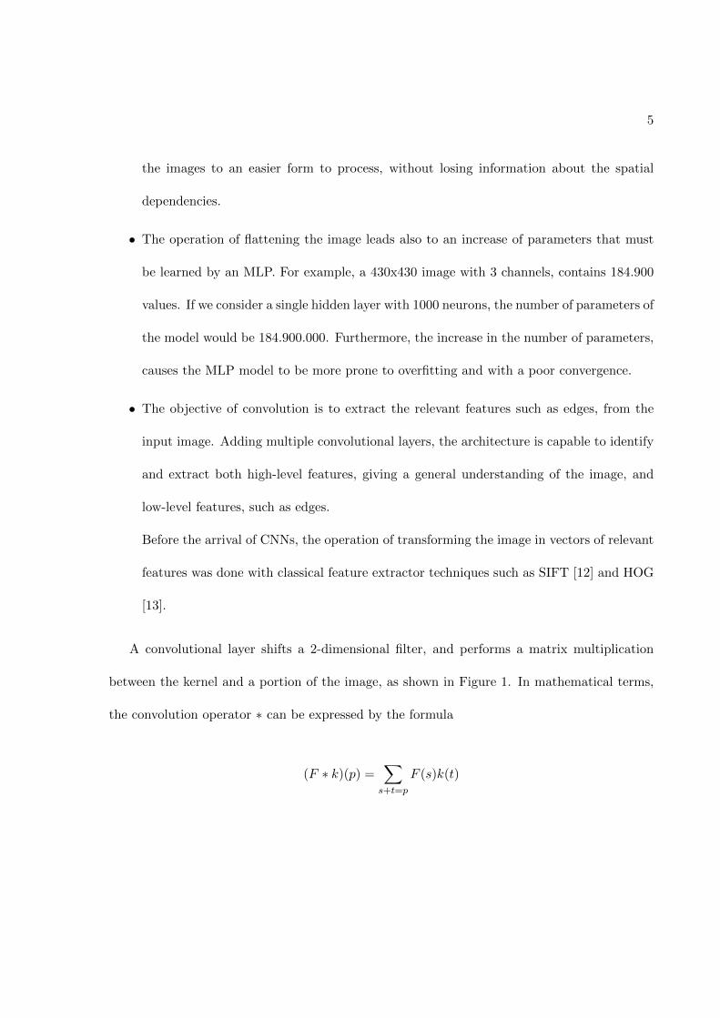
• The objective of convolution is to extract the relevant features such as edges, from the
input image. Adding multiple convolutional layers, the architecture is capable to identify
and extract both high-level features, giving a general understanding of the image, and
low-level features, such as edges.
Before the arrival of CNNs, the operation of transforming the image in vectors of relevant
features was done with classical feature extractor techniques such as SIFT [12] and HOG
[13].
A convolutional layer shifts a 2-dimensional filter, and performs a matrix multiplication
between the kernel and a portion of the image, as shown in Figure 1. In mathematical terms,
the convolution operator ∗ can be expressed by the formula
(F ∗ k)(p) =∑
s+t=p
F (s)k(t)

6
Figure 1: Example of convolution with a filter of size 3x3, stride 1 and no padding
where F : Z2 → R is a discrete function and k : [−r, r]2 ∩ Z2 → R is a discrete filter of size
(2r+1)2. A filter is a matrix of parameters which are learned by the architecture. It is relevant
to notice that the dimension of the filter, hence the number of parameters, is independent of
the dimension of the input.
To reduce the spatial size of the convolved features, hence reducing the computational
power required to process the data, a deep convolutional architecture also includes pooling
layers. These layers are also useful for extracting dominant features which are rotational and
positional invariant.
2.2 ResNet
As stated in the previous paragraph, the introduction of Convolutional Neural Networks
revolutionized the way of solving many tasks related to Computer Vision. The first deep con-
volutional architecture that produced state-of-the-art results in the task of image classification
7
for the ImageNet competition [14] was AlexNet [15]. This architecture was built using 5 con-
volutional and 3 fully-connected layers. Despite the good results obtained by this architecture,
a study showed that adding more layers would create a more complex function, increasing
the probability of overfitting, even if some regularization techniques (such as dropout [16] or
l2-norms) are applied.
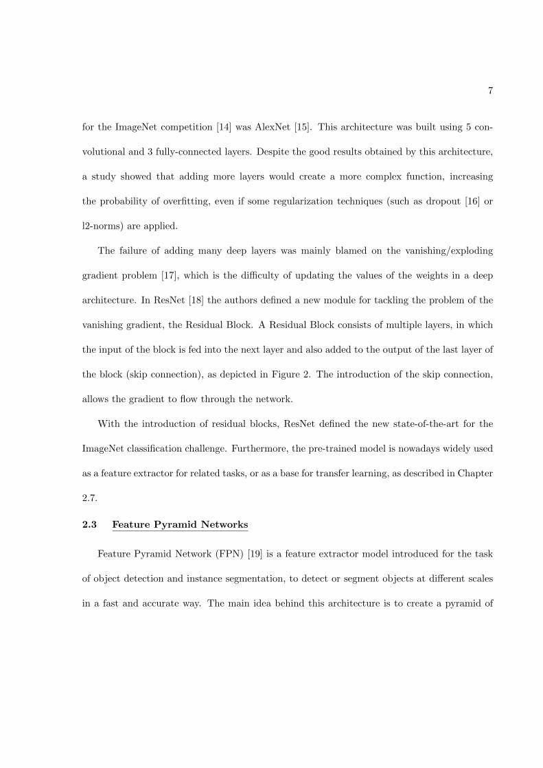
The failure of adding many deep layers was mainly blamed on the vanishing/exploding
gradient problem [17], which is the difficulty of updating the values of the weights in a deep
architecture. In ResNet [18] the authors defined a new module for tackling the problem of the
vanishing gradient, the Residual Block. A Residual Block consists of multiple layers, in which
the input of the block is fed into the next layer and also added to the output of the last layer of
the block (skip connection), as depicted in Figure 2. The introduction of the skip connection,
allows the gradient to flow through the network.
With the introduction of residual blocks, ResNet defined the new state-of-the-art for the
ImageNet classification challenge. Furthermore, the pre-trained model is nowadays widely used
as a feature extractor for related tasks, or as a base for transfer learning, as described in Chapter
2.7.
2.3 Feature Pyramid Networks
Feature Pyramid Network (FPN) [19] is a feature extractor model introduced for the task
of object detection and instance segmentation, to detect or segment objects at different scales
in a fast and accurate way. The main idea behind this architecture is to create a pyramid of

8
Figure 2: Residual Block introduced in ResNet
feature maps (multi-scale feature maps) which showed significant improvements compared to
the regular feature maps in various tasks, such as object detection and segmentation.
FPN is composed of two paths:
• The Bottom-Up path that is a convolutional network for feature extraction, such as
ResNet. Going deeper into the model decreases the spatial resolution but increases the
semantic information for each layer.
• The Top-Down path is used to construct higher resolution layers from a semantic rich
layer.
The bottom-up path is responsible for producing dense feature vectors at different resolu-
tions. A dense feature vector is built using the output of a convolution module, that we call

9
Ci, which is used in the top-down path. In the top-down path, the i-th layer takes as input the
sum of Ci (convolved with a 1 × 1 convolution filter) and the output of the previous layer in
the path, upsampled by 2. The output of the different layers in the top-down path is also the
output of the architecture.
A similar architecture is the Panoptic Feature Pyramid Network [20]. The only difference
is in the top-down path. In particular, the outputs of the convolution module are convolved
with a 2× 2 convolution filter and upsampled by 2 until it reaches 1/4 scale. At this point, the
top-down path consists of the element-wise summation of the new feature maps. Figure 3 and
Figure 4 show an example of the two architectures.
2.4 Region of Interest Pooling
The Region of Interest (RoI) Pooling layer was first introduced in [21] to solve the burden
of dealing with bounding boxes of different sizes in the task of object detection. This layer
produces a fixed-sized feature map from inputs with different sizes, applying max-pooling on
the inputs.
A RoI pooling layer takes two inputs:
• A feature map obtained from a Convolutional Model
• N bounding box (BB) coordinates representing the ’regions of interest’ in the image,
usually generated by a Region Proposal network.
For each bounding box, the RoI pooling layer crop the values of the input feature-map
related to that region and convert the cropped section to a fixed-sized feature map. The most

10
Figure 3: Feature Pyramid Network
Figure 4: Panoptic Feature Pyramid Network

11
important feature of this layer is its capability of producing a fixed-size representation. The
size of the new representation is a parameter of the layer itself, hence it is independent both
from the dimension of the input feature map and from the RoI size.
Another parameter required by the RoI layer is the spatial scale. In a region proposal
network, the RoIs are generated based on the input image size. Hence, there is a need to
rescale them to extract the relevant region from the input feature map. For example, with an
input image of size 160 × 160 and a feature map of size 20 × 20, the spatial scale parameter
value is 0.125.
The operations carried out by the RoI pooling layer can be summarized as:
• The rescaling phase, which consists of dividing each BB coordinate by k (the spatial scale
parameter) and take the integer part, obtaining the new coordinates relative to the input
feature map.
• The operation of quantization, in which the cropped part of the feature map is divided
into bins, resulting in a n× n grid, and from each bin, the maximum or average value is
extracted. This results in a fixed-sized feature map relative to the RoI.
Figure 5 shows the process of applying RoI pooling for a single RoI.
An alternative to the RoI Pooling layer is the RoI Align layer [22]. This last method rescales
the bounding boxes more accurately with the following process
• The rescaling phase, that divides each BB coordinate by k, without rounding up

12
Figure 5: Example of RoI Pooling
• The quantization, in which the cropped feature map is divided into bins. For each bin
are selected 4 points using bilinear interpolation, then the maximum or average value is
extracted from these 4 points.
RoI Align is usually preferred to RoI Pooling when dealing with image segmentation because
it does not introduce the misalignment between the RoI and the extracted features.
2.5 Face Alignment
Face alignment, also known as face normalization, is the process of identifying landmarks
in images containing human faces, and to use those landmarks to obtain a new face image such
that the eyes are aligned and the face is centered. This result is accomplished through scaling,
rotating, and translating the input image.

13
Face alignment has been proved to be beneficial for the tasks of face recognition and ex-
pression recognition [23] because reduces the variations in face scale and in-plane rotations [24].
Two main types of face alignment exist:
• 3D-alignment defines a 3D reference landmark model, and transform the input image in
such a way that the landmarks of the input image match the landmarks in the 3D model
• 2D-alignment, is a simpler alignment method that relies on the scale, rotation and
translation of the input image based on the detected facial landmarks
The process of the 2D face alignment can be summarized as:
• Face detection and Landmark Localization, which consists of determining the loca-
tion of the face (or faces) in the input image and to extract localized landmark coordinates
(usually 5, 44 or 64). Classical face detection algorithms are Haar Cascades Classifier [25]
or Histogram of Oriented Gradients (HOG) [13].
A widely used DNN based face and landmark detection model is Multi-Task CNN (MTCNN)
[26] which employs multi-task learning and a cascade of learners to detect facial landmarks.
• Image warping and transformation is the last phase, and consists of warping and
transforming the input image to an output coordinate space, given a set of facial land-
marks.
There are different types of transformations that can be applied in this phase. In our work,

14
Figure 6: Landmark detection and alignment process
we will use the similarity transform [27] which is a composition of rotation, translations,
and magnifications. The points in the new image are defined by the formulas
X = s ∗ x ∗ cos(rotation)− s ∗ y ∗ sin(rotation) + a1
Y = s ∗ x ∗ sin(rotation) + s ∗ y ∗ cos(rotation) + b1
in which s is the scale factor, x and y are the translation parameters, rotation is the angle
in counter-clockwise as radians and the homogeneous transformation matrix is defined as
a0 b0 a1
b0 a0 b1
0 0 1
Figure 6 shows an example of the alignment process.

15
2.6 Optimization
Optimization is one of the core components of Machine Learning. ML algorithms aim at
building an optimization model that is capable of learning the parameters in the objective
function from the data. The classic optimization method for DNNs is Stochastic Gradient
Descent (SGD) [28] and its variants, with the backpropagation algorithm. SGD is a first-order
optimization method that iteratively travels down the slopes of the objective function until a
minimum is reached. At the end of an iteration of SGD, the backprop algorithm is used to
propagate the gradient updates in the network.
With Vanilla SGD, however, it is easy to fall in local minima or saddle point, often present
in the objective function. For this reason, momentum is usually added to SGD. Momentum
[29] is used to accumulate the gradients of the past steps, which will be used to determine the
weights’ update for the current step. This has been proved to increase the convergency speed
and to partially solve the problem of the optimization algorithm being stuck. The quantity of
gradient to inject in the network is regulated by the learning rate (LR), which determines the
step size of each iteration. A small value of the LR could lead to slow convergence while a high
LR may not lead to convergence at all.
Some recent methods introduced the capability of adapting the learning rate based on some
statistics. For example, RMSProp [30] stores the moving average of the square of the previous
gradients and divides the learning rate by the root of the mean square. This allows keeping
learning even if the value of the gradients is very small. Another widely used optimization

16
algorithm is Adam [31]. This method combines momentum and RMSProp and has been proved
to provide good performances for a wider range of learning rates.
2.7 Transfer Learning
Transfer Learning [32] is a widely used machine learning technique where a model which
has been trained on a task can be used as a starting point for a similar task. There are several
reasons why this technique has become popular and widely used
• Data requirement: DL models usually require a huge amount of high-quality annotated
data, which is not often available. With transfer learning, the model may be fine-tuned
in a smaller dataset producing high-quality results.
• Computation: DL techniques are known to be computationally intensive. With transfer
learning, we can save hours of computations without incurring in a decay of the results.
• Overfitting: The high number of parameters in a DL model can lead to an increase in
variance which leads to a low generalization capability. This problem can be leveraged
relying upon information from a related domain. z
• Model features: Some of the features learned by a DL model can be transferred to
another domain without relevant modifications.

CHAPTER 3
PREVIOUS WORK
In this chapter, we present some of the current works in AU detection which we have taken
as inspiration to develop our model. In recent years, Deep Learning approaches have dominated
the scene on multiple CV tasks. In Facial Action Unit detection, the first Deep Learning based
work that achieved considerable results, was developed in 2014. Since then, most of the works
are based on deep neural networks.
3.1 Deep Region and Multi-label Learning for Facial Action Unit Detection
Deep Region and Multi-Label Learning (DRML) [33] is one of the first Convolutional Neural
Network based model for AU recognition. The authors address two main problems in AU
recognition:
• Region Learning (RL) identify the sparse facial regions in which the AUs are active,
to improve detection performance. A particular example of RL is Patch Learning, which
consists of dividing the face image into uniform patches and train a model to assign a
value of importance to each patch.
• Multi-Label Learning (ML) is a consequence of the strong correlation between some
AUs. Previous works on AU detection extracts the correlation information from either
FACS heuristics or ground truth labels and uses them as input to the model. On the other
17

18
hand, the authors enforce the model to learn those correlations without prior knowledge
of the correlation between AUs.
The main component introduced in the model is the region layer, whose main function is
to identify the patches considered relevant for detecting the AUs. The region layer takes as
input the feature map produced by the first convolutional layer and divides into 8× 8 patches.
Each patch is fed into a second convolutional layer and then summed to the original patch.
The new re-weighted patches are then concatenated, resulting in a weighted feature map of the
same size as the input. The use of the region layer shows an improvement in identifying AU
discriminative regions compared to a standard CNN, such as AlexNet or ConvNet.
3.2 EAC-Net: Deep Nets with Enhancing and Cropping for Facial Action Unit
Detection
The Enhancing And Cropping (EAC) network [34], is based on a VGG [35] network, in
which the following layers are also added:
• Enhancing Layers are attention layers whose aim is to give more importance to the
regions of the image that are associated with the AUs. This attention layer is implemented
as a special type of skip connection between the input and the output of two groups of
convolution in the backbone model.
In detail, the output feature map of a group of convolutions is multiplied element-wise
by a handcrafted attention map and in parallel processed by the convolutional layers of
the next group. The two output feature maps are then fused by element-wise summation.

19
Figure 7: High-levek overview of the backbone model with Enhancing Layers
This process is repeated for two consecutive groups of convolutional layers. Figure 7 gives
a high-level overview of this module.
• Cropping layers are used to learn features for specific AUs. This module is composed
of 20 branches in which each branch takes as input the cropped part of the output feature
map of the enhanced VGG. The cropped region is the rescaled center of the 20 AU centers
used in the attention map of the enhancing layers.
Each branch upsamples the cropped feature map which is then fed into a convolutional
layer. The outputs of the convolutional layers are concatenated and processed by a FC
network to produce the final prediction.
In subsequent work, the author included temporal information to the network, adding two
LSTM layers at the end of the previous model, before the dense layer used for the prediction.
EAC and EAC with LSTM achieved good results compared to previous works on AU detection,
particularly when the temporal information is introduced in the network.

20
3.3 Joint Facial Action Unit Detection and Face Alignment
In Deep Adaptive Attention for Joint Facial Action Unit Detection and Face Alignment
[36], the authors defined a deep neural network (JAA-Net) that jointly estimates AUs and
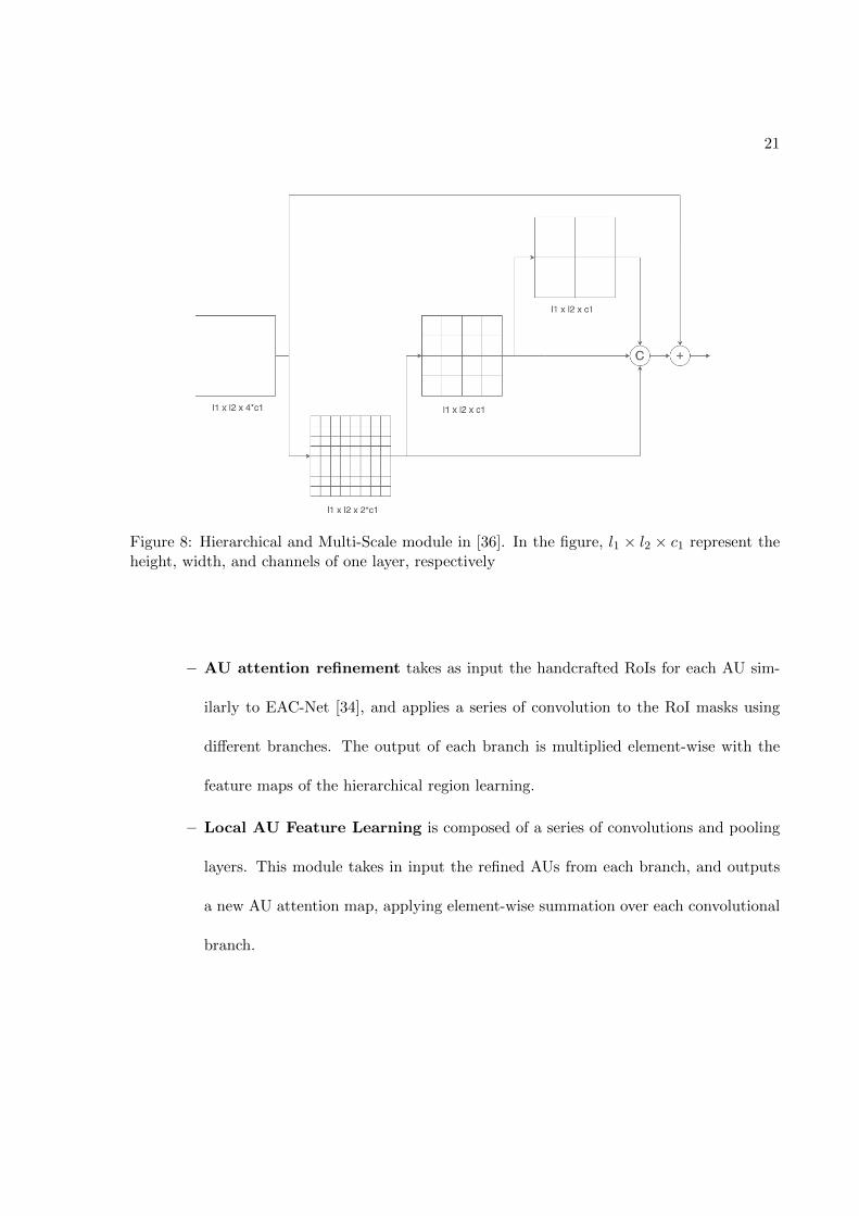
facial landmarks (face alignment). JAA-Net consists of the following modules:
• Hierarchical and multi-scale region learning is used to extract features at different
scales. Similarly to DRML [33], this layer aims at sharing the filter weights within patches
with different weights assigned to each patch.
This module is composed of an input layer and three hierarchical convolutional layers.
The multi-scale version stands for how the input of a convolution layer is modeled. In
particular, the intermediate 8×8, 4×4, and 2×2 patches of the second, third and fourth
convolutional layers are the result of convolution on corresponding patches in the previous
layer, input, first and second, respectively. The outputs of the three intermediate layers
are concatenated, and the final result is summed element-wise with the output of the
input layer. In Figure 8 is shown the structure of the hierarchical and multi-scale module.
• Face alignment estimates the locations of facial landmarks and generates the initial
attention maps that will be used in the next module. This module includes three convo-
lutional layers and a fully connected layer with 2 hidden layers.
• Adaptive attention learning is used to refine the initial AUs’ attention maps and
consists of two steps:
21
Figure 8: Hierarchical and Multi-Scale module in [36]. In the figure, l1 × l2 × c1 represent theheight, width, and channels of one layer, respectively
– AU attention refinement takes as input the handcrafted RoIs for each AU sim-
ilarly to EAC-Net [34], and applies a series of convolution to the RoI masks using
different branches. The output of each branch is multiplied element-wise with the
feature maps of the hierarchical region learning.
– Local AU Feature Learning is composed of a series of convolutions and pooling
layers. This module takes in input the refined AUs from each branch, and outputs
a new AU attention map, applying element-wise summation over each convolutional
branch.

22
To estimate probabilities of the AUs occurrences, the output feature maps of the face align-
ment and the hierarchical and multi-scale region learning are concatenated together and fed
into a FC network with two hidden layers.
3.4 Facial Action Unit Detection Using Attention and Relation Learning
In Facial Action Unit Detection Using Attention and Relation Learning [37], the authors
defined a deep learning framework (ARL) based on attention and relation learning for AU
detection. ARL is composed of 4 modules:
• Hierarchical and Multi-Scale region learning, as defined in JAA-Net [36].
• Channel-Wise Learning consists of a multi-branch architecture whose aim is to select
AU related features. For each action unit, the output of the region learning is fed into a
convolutional layer and pooled. This process produces a vector of channel-wise attention
weights. This vector is multiplied with the output of the convolution, obtaining a channel-
wise weighted feature.
• Spatial Attention learning which takes as input the channel-wise weighted feature
and process it with a convolutional layer, obtaining a spatial pixel-wise feature map. The
feature map is convolved with a single-channel convolutional layer and a sigmoid function
is applied, obtaining an initial spatial attention weight.
• Pixel-Level Relation Learning module captures the dependencies at pixel-level used
to refine spatial pixel-wise attentions. This module consists of a Conditional Random
Field [38] which takes as input the spatial attention weight and the convolved output

23
of the Channel-Wise learning module, obtaining a refined spatial attention weight. The
result is then multiplied with a new convolved version of the output of the Channel-Wise
module.
Finally, the output of the Pixel-Level Relation learning module is processed by a FC module
to predict the AUs’ occurrence.
CHAPTER 4
MODEL STRUCTURE
In this chapter, we give an in-depth description of the proposed architecture. In particular,
we explain the face alignment and Region of Interest extraction processes. Then, we describe
the Feature Pyramid Network and how this has been integrated with the Region of Interest
pooling module to solve the problem of AU detection.
4.1 Model Overview
As depicted in Figure 10, our architecture is composed of two main branches: the first one
consists of creating an aligned representation of the input image, which is then fed into the
Feature Pyramid Network that produces the encoding of the image, as detailed in Section 4.2.
We choose to use this structure because of its capability of extracting global features at different
scales, which has been proved to be beneficial for detecting AUs [36; 37]. The features extracted
by the FPN are fed into the Region of Interest module.
The second branch generates the bounding boxes for the Regions of Interest, which in this
case consists of regions of the face that are relevant to detect the different action units. The
Region of interest module consists of a multi-branch architecture that processes a feature map
differently based on the location of the occurrence of the AU in the face. The main purpose
of this module is to extract the local features related to the pre-defined bounding boxes. More
details are given in Section 4.3.
24

25
In this work, we aim at detecting 8 action units, shown in Figure 9, which are AU1, AU2,
AU4, AU6, AU9, AU12, AU25, AU26. Since the reference action units are centered in different
regions of the face, we choose to partition them based on the portion of the face in which they
occur. In particular, we defined 3 different face regions:
• Upper face which contains the eyes and the forehead
• Middle face is composed of the cheeks and the nose
• Lower face includes the mouth and the chin
4.1.1 Landmark Localization and Face Alignment
The first step is the detection of 64 facial landmarks that are used to align the image and to
create the bounding boxes related to the RoIs. In particular, the process of aligning the image
aims at normalizing the image in terms of scale and rotation, such that the position of the eyes
does not change in all the images of the datasets.
The facial landmarks are computed using the neural network based model described in [41]
and available in PyTorch [42]. This model is capable of providing reliable landmarks also in
case of partial occlusion of the face. After retrieving the facial landmarks, we align the image
using similarity transformation, as previously described in Section 2.5.
The identified landmarks, together with 64 reference landmark positions, are used to esti-
mate the transformation matrix which is applied to the input image. The result consists of
the cropped, rotated, and resized input image, with a fixed size of 160× 160 pixels. Figure 11
shows the process of landmark localization and alignment.

26
(a) AU1-Inner Brow Raiser (b) AU2-Outer Brow Raiser (c) AU4-Brow Lowerer
(d) AU6-Cheek Raiser (e) AU9-Nose Wrinkler (f) AU12-Lip Corner Puller
(g) AU25-Lips Part (h) AU26-Jaw Drop
Figure 9: Examples of the AUs in DISFA [39; 40]

27
Figure 10: Overview of the complete architecture
Figure 11: Landmark localization and face alignment process

28
Face portion AUs Number of RoIs
Upper 1, 2, 4, 6 5
Middle 9 2
Lower 12, 25, 26 4
TABLE II: Regions of Interests and face portion
4.1.2 Creation of the Regions of Interest
To determine the Regions of Interests, we first define the locations of the centers of the
AUs. Subsequently, we guide the creation of the bounding boxes related to the RoIs based on
the facial landmarks detected as described in the previous section.
More in detail, we defined a variable number of RoIs for each part of the face, as detailed
in Table II. Since we are extracting the bounding boxes taking into consideration the relative
position of the AU centers’ with respect to multiple facial landmarks, the bounding boxes are
dynamically defined and adapted to the face. Figure 12 shows the RoIs extracted for a single
image.
4.2 Feature Pyramid Network Module
The encoder portion of our architecture is inspired by the Panoptic Feature Pyramid Net-
work described in Section 2.3, and it is used to extract features at different resolutions. The
input of this network is an RGB image of size 160× 160× 3. The bottom-up path, which is the
backbone of the network, consists of a ResNet-50 architecture. More in detail, this backbone
is a collection of 4 groups of convolutions, preceded by a stem module composed of a 7 × 7
convolution and a 3 max-pooling layer, as described in the Table III.

29
Figure 12: Example of the extracted RoIs. In red, green and blue we show the bounding boxesof the upper, middle and lower face, respectively
Layer Name Output Size Operations
conv1 64× 1/4× 1/47× 7, 64, stride 2
3× 3 max pool, stride 2
conv2 256× 1/4× 1/4
1× 1, 643× 3, 641× 1, 256
× 3
conv3 512× 1/8× 1/8
1× 1, 1283× 3, 1281× 1, 512
× 4
conv4 1024× 1/16× 1/16
1× 1, 2563× 3, 2561× 1, 1024
× 6
conv5 2048× 1/32× 1/32
1× 1, 5123× 3, 5121× 1, 2048
× 3
TABLE III: ResNet-50. The fractions 1/4, 1/8, 1/16 and 1/32 refer to the height and widthratios with respect to the input image size

30
Figure 13: Feature Pyramid Network used in our architecture
In the top-down path, the output features of each group are fed into an upsampling module,
composed by a 3× 3 convolution, batch normalization, ReLu, and 2× bilinear upsampling, as
it is illustrated in Figure 13. From the deepest level of the FPN (at 1/32 scale), we perform
three upsampling stages to yield a feature map at 1/4 scale. This process is repeated for all the
remaining feature maps, with progressively fewer upsampling stages. The upsampled features
are then summed element-wise generating the output feature map with 128 channels at 1/4
scale, which will be used as input for the RoI module, as explained in Section 4.3. Figure 13,
shows the details of the FPN model.
4.3 Regions of Interest Module
The RoI module is used to extract local features related to the AUs located in different
regions of the face, and to estimate the presence of the AUs for that portion of the face.

31
Since we split the AUs based on their location of occurrence in the face, i.e., upper, middle,
and lower part of the face, we define three different branches:
• Upper Branch extracts the local features of the AUs that occurs in the upper region of
the face. Particularly, the eyes, the forehead, and between the eyebrows.
• Middle Branch takes into consideration the middle part of the face. We are interested
in detecting the AU related to the cheeks’ movement.
• Lower Branch is tasked with the extraction of the features for the AUs in the lower part
of the face. More in detail, we defined the RoIs to extract features related to the mouth,
the chin, and the corners of the lips.
Each branch takes as input the multi-scale feature map produced by the FPN module and
outputs a vector of estimations for the AUs related to that branch.
A branch consists of a RoI Align layer, described in Section 2.4, that extracts the local
features for each of the bounding boxes, and produces a fixed-size feature map. The output size
of this layer is #RoIs×128×pooling size×pooling size. These maps are then concatenated on
the second dimension and average pooling is applied, before feeding the vector feature map into
the bottleneck of each branch. Each bottleneck module is composed of a FC network, with 3
hidden layers. The last layer has a Softmax activation function which generates the estimation
for the AUs related to that specific branch.Figure 14 shows the details for this module.

32
Figure 14: Overview of the Region of Interest module
CHAPTER 5
TRAINING AND VALIDATION
This chapter gives more details about the datasets that we used to train and validate the
model, and the training and validation procedures applied.
5.1 Datasets
To train and validate the model, we used five different datasets:
• The VGGFace2 [43] dataset is a face-recognition dataset with more than 3.3 million
face images over more than 9,000 entities. It contains subjects with an equal gender
distribution and with a variety of ethnicities and ages. The images are captured ”in the
wild” such that the images are exposed to head pose variations, different lighting, and
occlusion conditions.
• The Extended Cohn-Kanade (CK+) [44; 45] dataset is one of the most well known
laboratory-controlled databases for Facial Expression Recognition and AU recognition.
The dataset contains 593 video sequences from 123 subjects. The duration of each se-
quence spans from 10 to 60 frames, and it starts from a neutral face to the peak expression.
Since the AU is provided for each sequence, usually the last three frames are extracted
along with the first frame (neutral expression).
• The UNBC-McMaster shoulder pain expression [46] database contains videos of
subjects who were suffering from shoulder pain, while they were performing some actions.
33

34
This dataset contains 200 sequences from 25 subjects. Each frame has been coded by
certified FACS coders, resulting in a total of around 47,000 coded frames.
• The Compound of Facial Expression Emotions (CFEE) [10], is a database of
compound emotions images, i.e., emotions constructed by combining basic emotions. The
authors defined a total of 21 compounds and basic emotions. The dataset is a collection of
230 subjects with around 21 images for each one, for a total of 4,816 FACS coded frames.
• The DISFA [39; 40] database, is one of the main benchmark datasets in AU recognition.
It is a collection of 27 sequences, with around 4,800 FACS coded frames for each sequence,
from 27 subjects. Each frame is labeled with AUs intensities ranging from 0 to 5. The 8
coded AUs are AU1, AU2, AU4, AU6, AU9, AU12, AU25, and AU26.
5.2 Training and Validation
In Section 2.7, we stated that transfer learning is a well-known method that helps the model
to improve generalization and speed up convergence. In our case, we initialize the weights of
the ResNet backbone with the weights obtained from training it on the VGGFace2 [43] dataset
for face recognition. The weights that we used are publicly available in [47].
The second training phase aims at fine-tuning the full model for recognizing the facial action
units. Each aligned image of size 160 × 160 is normalized in the same way as the pre-trained
backbone with the values shown in Table IV.
At training time we also apply some data augmentation techniques, to increase and diversify
the available data, and to improve the robustness of the model. We limited the augmentation to
variation in color and flipping to avoid distortion of the face in the input image and to simulate

35
Channel µ σ
R 0.485 0.229
G 0.456 0.224
B 0.406 0.225
TABLE IV: Normalization values (mean and standard deviation) for each channel
events such as illumination variations and occlusions. In particular, the training dataset has
been augmented using:
• Horizontal flip which flips the image horizontally. Since the AUs are symmetrical,
flipping the image allows us to increase the amount of training data without losing infor-
mation on the location of the action units
• Color Jitter performs random brightness, contrast, hue, and saturation variations so
that the model would be more robust to these variations at inference time
• Cutout [48] consists of masking out a random part of the input image. This technique
simulates occluded examples, encouraging the model to take into consideration a more
diverse set of features for classifying images. For example, to classify a car, the model
would be enforced to look at other details of the image, instead of just focusing on the
wheels.
To reduce the imbalance of the training data towards neutral samples, i.e. faces without
visible action units, and to increase the diversification of the data, which is reduced by the

36
(a) Occurrence rate of Action Units (b) Occurrence rate of Neutral Faces
Figure 15: Occurrence rates of AUs and Neutral Faces in DISFA
similarity of subsequent frames, we sub-sampled the images with neutral faces, including in the
training data 1 frame over 5.
To validate the model, we performed 3-fold cross-validation on the DISFA dataset, splitting
the data based on the subjects. In particular, we used the splits provided by [36]. Splitting
the data based on the subjects force the model to be as much subject-independent as possible.
Figure 15 shows the distribution of AUs and neutral faces on the DISFA dataset.
The training data is then composed of the images in CK+, UNBC and CFEE, and the
training folds of the DISFA dataset. Figure 16 shows the AUs’ and neutral faces’ distributions
on the training data.

37
(a) Occurrence rate of Action Units (b) Occurrence rate of Neutral Faces
Figure 16: Occurrence rates of AUs and Neutral Faces in the training data
5.3 Loss Function
Facial Action Unit detection is a multi-label classification problem because multiple AUs
can occur simultaneously in an image. For this reason, we used a weighted multi-label binary
cross-entropy loss function with sigmoid activation:
EBCE = − 1
nau
nau∑i=1
wi[pi log(pi) + (1− pi) log(1− pi)]
where
• pi is the ground truth probability of occurrence of the i-th label (1 or 0)
• pi represents the predicted probability of occurrence
• nau is the total number of action units

38
• wi is the weight introduced to alleviate the data imbalance. Particularly, we set
wi =(1/ri)nau∑naui=1(1/ri)
where ri is the number of samples with the i-th AU in the training data
Moreover, since some AUs are rarely present in the training data, the network is biased
towards absence for this AUs. To mitigate this problem, we introduce a multi-label Dice loss
[49], defined as:
EDice =1
nau
nau∑i=1
wi
(1− 2pipi + ε
p2i + pi2 + ε
)
where ε is a smoothing term. The Dice coefficient is also known as the F1-score, which is the
most popular metric for AU recognition, as described in Section 6. Introducing this coefficient,
we take into account the consistency between the loss function and the evaluation metric while
training out model.
The final loss function is
E = EBCE + λ ∗ EDice
where λ is an hyper-parameter used to weight the Dice loss.
The final network is trained for up to 2000 iterations in PyTorch [42], using Adam [31] to
optimize the objective function. We set the initial learning rate to 10−4, mini-batch size of 16,
and the λ factor for the Dice Loss has been set to 1.0.

CHAPTER 6
RESULTS
In this chapter, we introduce the evaluation metrics that have been used to validate the
model and we show the results and the ablation studies that we conducted.
6.1 Evaluation Metrics
• F1-score is the weighted average of the precision and recall. This metric is used in case of
imbalanced classification problems. In this work, since we are dealing with a multi-label
problem, we take into consideration the macro-averaged F1-score defined as
F1-score =1
nau
nau∑i=1
F1-scorei
=1
nau
nau∑i=1
2 ∗ pi ∗ ripi + ri
(6.1)
in which pi and ri refer to the precision and recall of the i-th class, respectively. These
measures are defined as
Precisioni = pi =TPi
TPi + FPi
Recalli = ri =TPi
TPi + FNi
(6.2)
where TP are the positive and correctly predicted samples, FP are the negative and
correctly predicted samples and the FN are the incorrectly predicted negative samples.
39

40
• Accuracy is the ratio between the correct predictions and the total number of predictions.
In a multi-label setting it’s computed as the mean of the accuracy for the single class
Accuracy =1
nau
nau∑i=1
Accuracyi
=1
nau
nau∑i=1
TPi + TNi
TPi + TNi + FPi + FNi
(6.3)
where TP, FP and FN are defined above and TN represents the correctly predicted neg-
ative samples.
6.2 Results on DISFA
We compare our method against some of the SOTA AU detection works under the same
3-fold cross-validation setting. In particular, we compare against the most recent deep learning
based models JAA [36] and ARL [37].
In Figure 17(a) we compare the averaged F1-score results with respect to the other methods.
The chart shows that our method outperforms the others, improving the results by 5.7% and 3%
with respect to JAA and ARL, respectively. For what concerns the F1-score for each single AU,
Figure 17(b) shows that the AU performances are fluctuating in all the methods. A possible
explanation for this behavior is that some AUs are easier to recognize with respect to others,
resulting in higher F1-score performance.
In terms of accuracy score, is possible to notice in Figure 18(a) that our method achieves
results analogous to the other reference methods. Even though we achieve the best accuracy
on AU1, AU2, AU4 and AU6 our method preforms slightly worse in terms of accuracy in the

41
(a) Average F1-score comparison
(b) Single AU F1-score comparison
Figure 17: F1-score comparison of JAA, ARL and Our method

42
prediction of the AUs located in the lower part of the face, as shown in Figure 18(b). Despite
this, we should notice that the accuracy score in a multi-label setting is less representative with
respect to the F1-score, since it doesn’t show the differences with respect to a biased model.
6.3 Ablation Studies
In this section, we conduct an analysis on the effects of various model components’ and
different training techniques that we applied. In Figure 19(a) we show the results obtained
removing some components of the model, in particular:
• ResNet refers to the pure ResNet-50 model of [1]
• In ResNet+RoI, we removed the FPN bottleneck representation
• FPN+RoI is the final model with FPN and RoI
All the different models have been trained and validated with the same settings, in terms of
training and validation data, hyperparameters, and validation procedure.
As we can see, the base model achieves the lowest result in terms of averaged F1-score.
A more in-depth analysis showed that the images with an active AU2 (outer brow raiser)
were mainly misclassified as AU1 (inner brow raiser). Including the Region of Interest pooling
improves the results by almost 3%. The best results are obtained when taking into consideration
the multi-scale features produced by the FPN, obtaining an increase of 6.4% and 3.5% compared
to the ResNet and Resnet with RoI pooling, respectively.

43
(a) Average Accuracy comparison
(b) Single AU Accuracy comparison
Figure 18: Accuracy comparison of JAA, ARL and Our method

44
(a) Average F1-score for different model configurations
(b) Average F1-score for different training configurations
In Figure 19(b) we show the results obtained training the final model under different training
settings. As we can notice, the pre-training phase of the model gives the best improvements in
terms of F1-score, bringing the F1 results from 49.0% to 58.7%.
Moreover, the model trained with the weighted loss and the dice loss produces the best
results. In particular, weighting the Binary Cross Entropy loss improves the prediction results
by 0.9%, and the introduction of the Dice loss leads to the best results, with an increase of
2.1% in terms of F1-score.
CHAPTER 7
CONCLUSIONS AND FUTURE DIRECTIONS
In this thesis, we designed a new deep learning based architecture for Facial Action Unit
detection that achieves results superior to other state-of-the-art models, in terms of F1-score.
We showed that the use of a Feature Pyramid network allows the model to learn features at
different scales, which has been proven to be beneficial for the task. Moreover, we defined a new
RoI pooling layer that extracts specific features for different regions of the face, and contribute
to the detection of AUs in a specific region in the face.
We evaluated the efficacy of our approach on the available benchmark dataset and motivated
our choices through ablation studies. There are possible developments for improving the current
model:
• Increasing training data might improve the robustness of the model, in particular for
the AUs that appear less frequently. As shown in Section 6.3, with a significant amount
of pre-training images the model provides better results.
• Enclose temporal information can be beneficial for the detection. AUs are related
to the movement of some muscle, hence they can be interpreted as a mutation of the
shape in a specific region of the face. Introducing temporal information would take into
consideration these variations in the face.
To do so, we can introduce an LSTM module before each FC layer on each branch, and
45

46
training the model with multiple subsequent images, instead of using a simple image. This
solution can be beneficial in terms of the obtained result, at the cost of longer training
time.
• As an alternative to training on sequence data, the use of a Neutral face as reference
frame might be beneficial for the model. With such an approach, the model can be
trained to learn the differences in aspects between a neutral face and the one in which
the AUs are occurring.
• The RoI extraction can lack precision in case of mispredicted facial landmarks, which is
mostly due to high head-pose variations. In such a case the model will not be able to
extract the correct face region that will be used for the AU detection. For this reason,
a manual annotation of the regions of interest made by experts could increase
the prediction accuracy of the model, but would also increase the cost related to the data
collection.

CITED LITERATURE
1. Menchetti, G., Chen, Z., Wilkie, D. J., Ansari, R., Yardimci, Y., and Cetin, A. E.:Pain detection from facial videos using two-stage deep learning. In 2019 IEEEGlobal Conference on Signal and Information Processing (GlobalSIP), pages 1–5,
Nov 2019.
2. Facial expressions of pain in lung cancer. Analgesia, 1(2), 1995.
3. Rubinow, D. R. and Post, R. M.: Impaired recognition of affect in facial expression indepressed patients. Biological Psychiatry, 31(9):947–953, 2020/03/24 1992.
4. Kapoor, A., Burleson, W., and Picard, R. W.: Automatic prediction of frustration.International Journal of Human-Computer Studies, 65(8):724 – 736, 2007.
5. Lankes, M., Riegler, S., Weiss, A., Mirlacher, T., Pirker, M., and Tscheligi,M.: Facial expressions as game input with different emotional feedbackconditions. In Proceedings of the 2008 International Conference on Advances inComputer Entertainment Technology, ACE ’08, page 253–256, New York, NY,USA, 2008. Association for Computing Machinery.
6. EKMAN, P.: Facial action coding system. 1977.
7. Lucey, P., Cohn, J. F., Prkachin, K. M., Solomon, P. E., and Matthews, I.: Painful data:The unbc-mcmaster shoulder pain expression archive database. In Face and Gesture2011, pages 57–64, 2011.
8. Pantic, M., Valstar, M. F., Rademaker, R., and Maat, L.: Web-based database for fa-cial expression analysis. In Proceedings of IEEE Int’l Conf. Multimedia and Expo(ICME’05), pages 317–321, Amsterdam, The Netherlands, July 2005.
9. Lucey, P., Cohn, J. F., Kanade, T., Saragih, J., Ambadar, Z., and Matthews, I.: The ex-tended cohn-kanade dataset (ck+): A complete dataset for action unit and emotion-specified expression. In 2010 IEEE Computer Society Conference on ComputerVision and Pattern Recognition - Workshops, pages 94–101, 2010.
47

48
CITED LITERATURE (continued)
10. Du, S., Tao, Y., and Martinez, A. M.: Compound facial expressions of emotion. Proceedingsof the National Academy of Sciences, 111(15):E1454–E1462, 2014.
11. LeCun, Y., Haffner, P., Bottou, L., and Bengio, Y.: Object recognition withgradient-based learning. In Shape, Contour and Grouping in Computer Vision,volume 1681 of Lecture Notes in Computer Science (including subseries LectureNotes in Artificial Intelligence and Lecture Notes in Bioinformatics), pages 319–
345. Springer Verlag, 1999. International Workshop on Shape, Contour and Group-ing in Computer Vision ; Conference date: 26-05-1998 Through 29-05-1998.
12. Lowe, D. G.: Distinctive image features from scale-invariant keypoints. Int. J. Comput.Vision, 60(2):91–110, November 2004.
13. Dalal, N. and Triggs, B.: Histograms of oriented gradients for humandetection. Computer Vision and Pattern Recognition, 2005. CVPR 2005. IEEEComputer Society Conference on, 1:886–893, 2005.
14. Deng, J., Dong, W., Socher, R., Li, L.-J., Li, K., and Fei-Fei, L.: ImageNet: A Large-ScaleHierarchical Image Database. In CVPR09, 2009.
15. Krizhevsky, A., Sutskever, I., and Hinton, G. E.: Imagenet classification with deep convolu-tional neural networks. In Advances in Neural Information Processing Systems 25,eds. F. Pereira, C. J. C. Burges, L. Bottou, and K. Q. Weinberger, pages 1097–1105.Curran Associates, Inc., 2012.
16. Srivastava, N., Hinton, G., Krizhevsky, A., Sutskever, I., and Salakhutdinov, R.: Dropout:A simple way to prevent neural networks from overfitting. J. Mach. Learn. Res.,15(1):1929–1958, January 2014.
17. Hochreiter, S.: The vanishing gradient problem during learning recurrent neuralnets and problem solutions. International Journal of Uncertainty, Fuzziness andKnowledge-Based Systems, 6(2):107–116, 1998.
18. He, K., Zhang, X., Ren, S., and Sun, J.: Deep residual learning for image recog-nition. In 2016 IEEE Conference on Computer Vision and Pattern Recognition(CVPR), pages 770–778, 2016.
19. Lin, T., Dollar, P., Girshick, R., He, K., Hariharan, B., and Belongie, S.: Feature pyramidnetworks for object detection. In 2017 IEEE Conference on Computer Vision andPattern Recognition (CVPR), pages 936–944, 2017.

49
CITED LITERATURE (continued)
20. Kirillov, A., Girshick, R., He, K., and Dollar, P.: Panoptic feature pyra-mid networks. In 2019 IEEE/CVF Conference on Computer Vision and PatternRecognition (CVPR), pages 6392–6401, 2019.
21. Girshick, R.: Fast r-cnn. In Proceedings of the 2015 IEEE International Conference onComputer Vision (ICCV), ICCV ’15, page 1440–1448, USA, 2015. IEEE ComputerSociety.
22. He, K., Gkioxari, G., Dollar, P., and Girshick, R.: Mask r-cnn. In 2017 IEEE InternationalConference on Computer Vision (ICCV), pages 2980–2988, 2017.
23. Mollahosseini, A., Chan, D., and Mahoor, M. H.: Going deeper in facial expression recogni-tion using deep neural networks. In 2016 IEEE Winter Conference on Applicationsof Computer Vision (WACV), pages 1–10, 2016.
24. Li, S. and Deng, W.: Deep facial expression recognition: A survey. IEEE Transactions onAffective Computing, PP, 04 2018.
25. Viola, P. and Jones, M.: Rapid object detection using a boosted cascade of sim-ple features. In Proceedings of the 2001 IEEE Computer Society Conference onComputer Vision and Pattern Recognition. CVPR 2001, volume 1, pages I–I, 2001.
26. Zhang, K., Zhang, Z., Li, Z., and Qiao, Y.: Joint face detection and alignment us-ing multitask cascaded convolutional networks. IEEE Signal Processing Letters,23(10):1499–1503, 2016.
27. Anonymous: Affine transform. https://scikit-image.org/docs/dev/api/skimage.
transform.html#skimage.transform.AffineTransform, 2018.
28. Rumelhart, D. E., Hinton, G. E., and Williams, R. J.: Learning Representations by Back-propagating Errors. Nature, 323(6088):533–536, 1986.
29. Sutskever, I., Martens, J., Dahl, G., and Hinton, G.: On the importance of initializa-tion and momentum in deep learning. In Proceedings of the 30th InternationalConference on Machine Learning, eds. S. Dasgupta and D. McAllester, volume 28of Proceedings of Machine Learning Research, pages 1139–1147, Atlanta, Georgia,USA, 17–19 Jun 2013. PMLR.

50
CITED LITERATURE (continued)
30. Tieleman, T. and Hinton, G.: Lecture 6.5—RmsProp: Divide the gradient by a running av-erage of its recent magnitude. COURSERA: Neural Networks for Machine Learning,2012.
31. Kingma, D. P. and Ba, J.: Adam: A method for stochastic optimization, 2014. citearxiv:1412.6980Comment: Published as a conference paper at the 3rd InternationalConference for Learning Representations, San Diego, 2015.
32. Tan, C., Sun, F., Kong, T., Zhang, W., Yang, C., and Liu, C.: A Survey on Deep TransferLearning: 27th International Conference on Artificial Neural Networks, Rhodes,
Greece, October 4–7, 2018, Proceedings, Part III, pages 270–279. 10 2018.
33. Zhao, K., Chu, W.-S., and Zhang, H.: Deep region and multi-label learning for facialaction unit detection. In The IEEE Conference on Computer Vision and PatternRecognition (CVPR), June 2016.
34. Li, W., Abtahi, F., Zhu, Z., and Yin, L.: Eac-net: Deep nets with enhancing and crop-ping for facial action unit detection. IEEE Transactions on Pattern Analysis andMachine Intelligence, 40(11):2583–2596, 2018.
35. Simonyan, K. and Zisserman, A.: Very deep convolutional networks for large-scale imagerecognition. In International Conference on Learning Representations, 2015.
36. Shao, Z., Liu, Z., Cai, J., and Ma, L.: Deep adaptive attention for joint facial action unitdetection and face alignment. In European Conference on Computer Vision, pages725–740. Springer, 2018.
37. Shao, Z., Liu, Z., Cai, J., Wu, Y., and Ma, L.: Facial action unit detection using atten-tion and relation learning. IEEE Transactions on Affective Computing, PP:1–1, 102019.
38. Lafferty, J. D., McCallum, A., and Pereira, F. C. N.: Conditional random fields: Prob-abilistic models for segmenting and labeling sequence data. In Proceedings of theEighteenth International Conference on Machine Learning, ICML ’01, pages 282–
289, San Francisco, CA, USA, 2001. Morgan Kaufmann Publishers Inc.
39. Mavadati, S. M., Mahoor, M. H., Bartlett, K., Trinh, P., and Cohn, J. F.: Disfa: A sponta-neous facial action intensity database. IEEE Transactions on Affective Computing,4(2):151–160, 2013.
51
CITED LITERATURE (continued)
40. Mavadati, S. M., Mahoor, M. H., Bartlett, K., and Trinh, P.: Automatic detection of non-posed facial action units. In 2012 19th IEEE International Conference on ImageProcessing, pages 1817–1820, 2012.
41. Bulat, A. and Tzimiropoulos, G.: How far are we from solving the 2d & 3d face align-ment problem? (and a dataset of 230,000 3d facial landmarks). In InternationalConference on Computer Vision, 2017.
42. Paszke, A., Gross, S., Massa, F., Lerer, A., Bradbury, J., Chanan, G., Killeen, T., Lin, Z.,Gimelshein, N., Antiga, L., Desmaison, A., Kopf, A., Yang, E., DeVito, Z., Raison,M., Tejani, A., Chilamkurthy, S., Steiner, B., Fang, L., Bai, J., and Chintala, S.:Pytorch: An imperative style, high-performance deep learning library. In Advancesin Neural Information Processing Systems 32, eds. H. Wallach, H. Larochelle, A.
Beygelzimer, F. d'Alche-Buc, E. Fox, and R. Garnett, pages 8024–8035. CurranAssociates, Inc., 2019.
43. Cao, Q., Shen, L., Xie, W., Parkhi, O. M., and Zisserman, A.: Vggface2: A dataset forrecognising faces across pose and age. In International Conference on AutomaticFace and Gesture Recognition, 2018.
44. Kanade, T., Cohn, J. F., and Yingli Tian: Comprehensive database for facial expressionanalysis. In Proceedings Fourth IEEE International Conference on Automatic Faceand Gesture Recognition (Cat. No. PR00580), pages 46–53, 2000.
45. Lucey, P., Cohn, J., Kanade, T., Saragih, J., Ambadar, Z., and Matthews, I.: The ex-tended cohn-kanade dataset (ck+): A complete dataset for action unit and emotion-specified expression. pages 94 – 101, 07 2010.
46. Lucey, P., Cohn, J. F., Prkachin, K. M., Solomon, P. E., Chew, S., and Matthews, I.:Painful monitoring: Automatic pain monitoring using the unbc-mcmaster shoulderpain expression archive database. Image and Vision Computing, 30(3):197 – 205,2012. Best of Automatic Face and Gesture Recognition 2011.
47. Anonymous: Pytorch face recognizer based on ’vggface2: A dataset for recognising facesacross pose and age. https://github.com/cydonia999/VGGFace2-pytorch, 2018.
48. DeVries, T. and Taylor, G.: Improved regularization of convolutional neural networks withcutout. 08 2017.

52
CITED LITERATURE (continued)
49. Milletari, F., Navab, N., and Ahmadi, S.-A.: V-net: Fully convolutional neural networksfor volumetric medical image segmentation. pages 565–571, 10 2016.

VITA
NAME Guglielmo Menchetti
EDUCATION
Master of Science in “Computer Science”, University of Illinois atChicago, May 2020, USA
Master of Science in “Computer Science and Engineering”, Politecnicodi Milano, December 2020, Italy
Bachelor’s Degree in ”Computer Science and Engineering””, Universitadegli Studi di Firenze, April 2017, Italy
LANGUAGE SKILLS
Italian Native speaker
English Full working proficiency
2017 - IELTS examination (7/9)
A.Y. 2018/20 - One Year of study abroad in Chicago, Illinois
A.Y. 2017/18 - Lessons and exams attended exclusively in English
SCHOLARSHIPS
Spring-Fall 2019 Research Assistantship (RA) position (10 hours/week) with full tuitionwaiver plus monthly stipend
Spring 2018 Italian scholarship for TOP-UIC students
53