multi channel software manual · if the sampling frequency is lower than twice the frequency of the...
TRANSCRIPT

Handyscope HS3
Instrument manualRev. 2.1
TiePie engineering

ATTENTION!
Measuring directly on the line voltage can be very dan-gerous.The outside of the BNC connectors at the Handy-scope HS3 are connected with the ground of the com-puter.Use a good isolation transformer or a differential probewhen measuring at the line voltage or at groundedpower supplies! A short-circuit current will flow if theground of the Handyscope HS3 is connected to a positivevoltage. This short-circuit current can damage both theHandyscope HS3 and the computer.
Despite the care taken for the compilation of this user manual, TiePieengineering can not be held responsible for any damages resulting fromerrors that may appear in this book.
Copyright c©2011 TiePie engineering. All rights reserved.
Contents
1 Safety 1
2 Declaration of confirmity 3
3 Introduction 53.1 Sampling . . . . . . . . . . . . . . . . . . . . . . . . 63.2 Sample frequency . . . . . . . . . . . . . . . . . . . . 7
3.2.1 Aliasing . . . . . . . . . . . . . . . . . . . . . 73.3 Digitizing . . . . . . . . . . . . . . . . . . . . . . . . 93.4 Signal coupling . . . . . . . . . . . . . . . . . . . . . 103.5 Probe compensation . . . . . . . . . . . . . . . . . . 10
4 Driver installation 134.1 Introduction . . . . . . . . . . . . . . . . . . . . . . . 134.2 Where to find the driver setup . . . . . . . . . . . . 134.3 Executing the installation utility . . . . . . . . . . . 13
5 Hardware installation 195.1 Power the instrument . . . . . . . . . . . . . . . . . 19
5.1.1 External power . . . . . . . . . . . . . . . . . 195.2 Connect the instrument to the computer . . . . . . . 20
5.2.1 Found New Hardware Wizard . . . . . . . . . 215.3 Plug into a different USB port . . . . . . . . . . . . 23
6 Front panel 256.1 CH1 and CH2 input connectors . . . . . . . . . . . . 256.2 GENERATOR output connector . . . . . . . . . . . 256.3 Power indicator . . . . . . . . . . . . . . . . . . . . . 25
7 Rear panel 277.1 Power . . . . . . . . . . . . . . . . . . . . . . . . . . 27
7.1.1 USB power cable . . . . . . . . . . . . . . . . 287.1.2 Power adapter . . . . . . . . . . . . . . . . . 29
7.2 USB . . . . . . . . . . . . . . . . . . . . . . . . . . . 297.3 Extension Connector . . . . . . . . . . . . . . . . . . 29
8 Specifications 318.1 Acquisition system . . . . . . . . . . . . . . . . . . . 31
Contents I

8.2 BNC inputs Ch1, Ch2 . . . . . . . . . . . . . . . . . 318.3 Trigger system . . . . . . . . . . . . . . . . . . . . . 328.4 Arbitrary Waveform Generator . . . . . . . . . . . . 328.5 Interface . . . . . . . . . . . . . . . . . . . . . . . . . 328.6 Power . . . . . . . . . . . . . . . . . . . . . . . . . . 338.7 Physical . . . . . . . . . . . . . . . . . . . . . . . . . 338.8 I/O connectors . . . . . . . . . . . . . . . . . . . . . 338.9 System requirements . . . . . . . . . . . . . . . . . . 338.10 Operating environment . . . . . . . . . . . . . . . . . 338.11 Storage environment . . . . . . . . . . . . . . . . . . 338.12 Certifications and Compliances . . . . . . . . . . . . 348.13 Package . . . . . . . . . . . . . . . . . . . . . . . . . 34
II

Safety 1When working with electricity, no instrument can guaran-tee complete safety. It is the responsibility of the personwho works with the instrument to operate it in a save way.Maximum security is achieved by selecting the proper in-struments and following save working procedures. Saveworking tips are given below:
• Always work according (local) regulations.• Work on installations with voltages higher than 25 V AC or
60 V DC should only be performed by qualified personnel.• Avoid working alone.• Observe all indications on the Handyscope HS3 before con-
necting any wiring• Check the probes/test leads for damages. Do not use them
if they are damaged• Take care when measuring at voltages higher than 25V AC
or 60 V DC.• Do not operate the equipment in an explosive atmosphere or
in the presence of flammable gases or fumes.• Do not use the equipment if it does not operate properly.
Have the equipment inspected by qualified service personal.If necessary, return the equipment to TiePie engineering forservice and repair to ensure that safety features are main-tained.
• Measuring directly on the line voltage can be very danger-ous. The outside of the BNC connectors at the Handy-scope HS3 are connected with the ground of the computer.Use a good isolation transformer or a differential probe whenmeasuring at the line voltage or at grounded power sup-plies! A short-circuit current will flow if the ground of theHandyscope HS3 is connected to a positive voltage. Thisshort-circuit current can damage both the Handyscope HS3and the computer.
Safety 1

2 Chapter 1

Declaration of confirmity 2TiePie engineeringKoperslagersstraat 378601 WL SneekThe Netherlands
EC Declaration of confirmity
We declare, on our own responsibility, that the product
Handyscope HS3-5MHzHandyscope HS3-10MHzHandyscope HS3-25MHzHandyscope HS3-50MHzHandyscope HS3-100MHz
for which this declaration is valid, is in compliance with
EN 55011:2009/A1:2010 EN 61000-6-1:2007
EN 55022:2006/A1:2007 EN 61000-6-3:2007
according the conditions of the EMC standard 2004/108/EC.
Sneek, 1-11-2010
ir. A.P.W.M. Poelsma
Declaration of confirmity 3

4 Chapter 2

Introduction 3Before using the Handyscope HS3 first read chapter 1 aboutsafety.
Many technicians investigate electrical signals. Though the mea-surement may not be electrical, the physical variable is often con-verted to an electrical signal, with a special transducer. Commontransducers are accelerometers, pressure probes, current clampsand temperature probes. The advantages of converting the physicalparameters to electrical signals are large, since many instrumentsfor examining electrical signals are available.The Handyscope HS3 is a portable two channel measuring instru-ment with Arbitrary Waveform Generator. The Handyscope HS3is available in several models with different maximum sampling fre-quencies: 5 MS/s, 10 MS/s, 25 MS/s, 50 MS/s or 100 MS/s. Thenative resolution is 12 bits, but user selectable resolutions of 8, 14and 16 bits are available too, with adjusted maximum samplingfrequency:
resolution Maximum sampling frequency
8 bit 100 MS/s
12 bit 5, 10, 25 or 50 MS/s, depending on model
14 bit 3.125 MS/s
16 bit 195 kS/s
Table 3.1: Maximum sampling frequencies
With the accompanying software the Handyscope HS3 can be usedas an oscilloscope, a spectrum analyzer, a true RMS voltmeter or atransient recorder. All instruments measure by sampling the inputsignals, digitizing the values, process them, save them and displaythem.
Introduction 5
3.1 Sampling
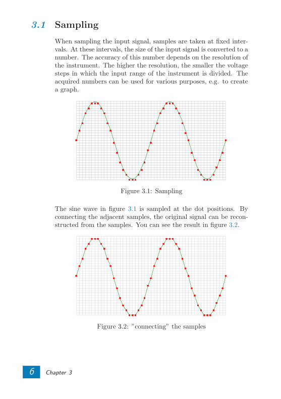
When sampling the input signal, samples are taken at fixed inter-vals. At these intervals, the size of the input signal is converted to anumber. The accuracy of this number depends on the resolution ofthe instrument. The higher the resolution, the smaller the voltagesteps in which the input range of the instrument is divided. Theacquired numbers can be used for various purposes, e.g. to createa graph.
Figure 3.1: Sampling
The sine wave in figure 3.1 is sampled at the dot positions. Byconnecting the adjacent samples, the original signal can be recon-structed from the samples. You can see the result in figure 3.2.
Figure 3.2: ”connecting” the samples
6 Chapter 3

3.2 Sample frequency
The rate at which the samples are taken is called the samplingfrequency, the number of samples per second. A higher samplingfrequency corresponds to a shorter interval between the samples.As is visible in figure 3.3, with a higher sampling frequency, theoriginal signal can be reconstructed much better from the measuredsamples.
Figure 3.3: The effect of the sampling frequency
The sampling frequency must be higher than 2 times the highestfrequency in the input signal. This is called the Nyquist fre-quency. Theoretically it is possible to reconstruct the input signalwith more than 2 samples per period. In practice, 10 to 20 sam-ples per period are recommended to be able to examine the signalthoroughly.
3.2.1 Aliasing
When sampling an analog signal with a certain sampling frequency,signals appear in the output with frequencies equal to the sum anddifference of the signal frequency and multiples of the samplingfrequency. For example, when the sampling frequency is 1000 Hzand the signal frequency is 1250 Hz, the following signal frequencieswill be present in the output data:
Introduction 7

Multiple of sampling frequency 1250 Hz signal -1250 Hz signal
...
-1000 -1000 + 1250 = 250 -1000 - 1250 = -2250
0 0 + 1250 = 1250 0 - 1250 = -1250
1000 1000 + 1250 = 2250 1000 - 1250 = -250
2000 2000 + 1250 = 3250 2000 - 1250 = 750
...
Table 3.2: Aliasing
As stated before, when sampling a signal, only frequencies lowerthan half the sampling frequency can be reconstructed. In thiscase the sampling frequency is 1000 Hz, so we can we only observesignals with a frequency ranging from 0 to 500 Hz. This meansthat from the resulting frequencies in the table, we can only seethe 250 Hz signal in the sampled data. This signal is called analias of the original signal.If the sampling frequency is lower than twice the frequency of theinput signal, aliasing will occur. The following illustration showswhat happens.
Figure 3.4: Aliasing
In figure 3.4, the green input signal (top) is a triangular signal witha frequency of 1.25 kHz. The signal is sampled with a frequency of1 kHz. The corresponding sampling interval is 1/1000Hz = 1ms.
8 Chapter 3
The positions at which the signal is sampled are depicted withthe blue dots. The red dotted signal (bottom) is the result of thereconstruction. The period time of this triangular signal appearsto be 4 ms, which corresponds to an apparent frequency (alias) of250 Hz (1.25 kHz - 1 kHz).
To avoid aliasing, always start measuring at the highest sam-pling frequency and lower the sampling frequency if required.
3.3 Digitizing
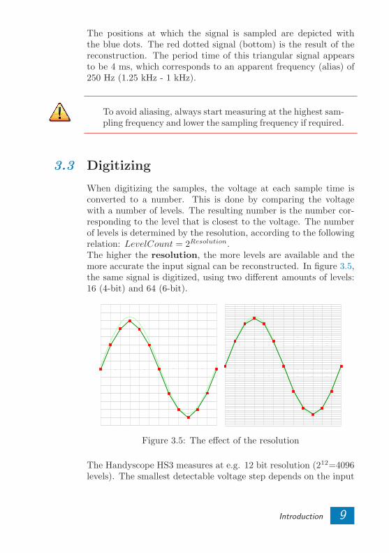
When digitizing the samples, the voltage at each sample time isconverted to a number. This is done by comparing the voltagewith a number of levels. The resulting number is the number cor-responding to the level that is closest to the voltage. The numberof levels is determined by the resolution, according to the followingrelation: LevelCount = 2Resolution.The higher the resolution, the more levels are available and themore accurate the input signal can be reconstructed. In figure 3.5,the same signal is digitized, using two different amounts of levels:16 (4-bit) and 64 (6-bit).
Figure 3.5: The effect of the resolution
The Handyscope HS3 measures at e.g. 12 bit resolution (212=4096levels). The smallest detectable voltage step depends on the input
Introduction 9

range. This voltage can be calculated as:
V oltageStep = FullInputRange/LevelCount
For example, the 200 mV range ranges from -200 mV to +200mV, therefore the full range is 400 mV. This results in a smallestdetectable voltage step of 0.400V/4096 = 97.65 µV.
3.4 Signal coupling
The Handyscope HS3 has two different settings for the signal cou-pling: AC and DC. In the setting DC, the signal is directly coupledto the input circuit. All signal components available in the inputsignal will arrive at the input circuit and will be measured.In the setting AC, a capacitor will be placed between the inputconnector and the input circuit. This capacitor will block all DCcomponents of the input signal and let all AC components passthrough. This can be used to remove a large DC component of theinput signal, to be able to measure a small AC component at highresolution.
When measuring DC signals, make sure to set the signalcoupling of the input to DC.
3.5 Probe compensation
The Handyscope HS3 is shipped with a probe for each input chan-nel. These are 1x/10x selectable passive probes. This means thatthe input signal is passed through directly or 10 times attenuated.
When using an oscilloscope probe in 1:1 the setting, thebandwidth of the probe is only 6 MHz. The full bandwidthof the probe is only obtained in the 1:10 setting
The x10 attenuation is achieved by means of an attenuation net-work. This attenuation network has to be adjusted to the oscillo-scope input circuitry, to guarantee frequency independency. This
10 Chapter 3

is called the low frequency compensation. Each time a probe isused on an other channel or an other oscilloscope, the probe mustbe adjusted.Therefore the probe is equiped with a setscrew, with which theparallel capacity of the attenuation network can be altered. Toadjust the probe, switch the probe to the x10 and attach the probeto a 1 kHz square wave signal. Then adjust the probe for a squarefront corner on the square wave displayed. See also the followingillustrations.
Figure 3.6: correct
Figure 3.7: under compensated
Figure 3.8: over compensated
Introduction 11

12 Chapter 3

Driver installation 4
Before connecting the Handyscope HS3 to the computer, thedrivers need to be installed.
4.1 Introduction
To operate a Handyscope HS3, a driver is required to interfacebetween the measurement software and the instrument. This drivertakes care of the low level communication between the computerand the instrument, through USB. When the driver is not installed,or an old, no longer compatible version of the driver is installed, thesoftware will not be able to operate the Handyscope HS3 properlyor even detect it at all.The installation of the USB driver is done in a few steps. Firstly,the driver has to be pre-installed by the driver setup program. Thismakes sure that all required files are located where Windows canfind them. When the instrument is plugged in, Windows will detectnew hardware and install the required drivers.
4.2 Where to find the driver setup
The driver setup program and measurement software can be foundin the download section on TiePie engineering’s website and on theCD-ROM that came with the instrument. It is recommended toinstall the latest version of the software and USB driver from thewebsite. This will guarantee the latest features are included.
4.3 Executing the installation utility
To start the driver installation, execute the downloaded driversetup program, or the one on the CD-ROM that came with theinstrument. The driver install utility can be used for a first time
Driver installation 13
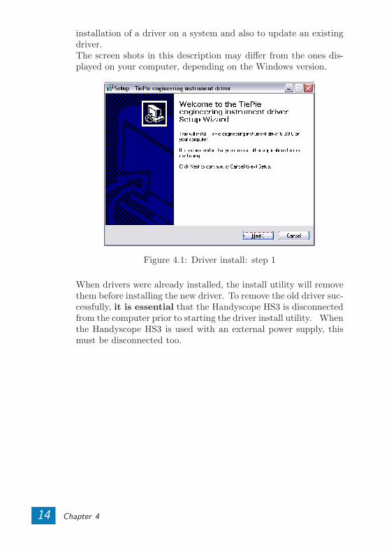
installation of a driver on a system and also to update an existingdriver.The screen shots in this description may differ from the ones dis-played on your computer, depending on the Windows version.
Figure 4.1: Driver install: step 1
When drivers were already installed, the install utility will removethem before installing the new driver. To remove the old driver suc-cessfully, it is essential that the Handyscope HS3 is disconnectedfrom the computer prior to starting the driver install utility. Whenthe Handyscope HS3 is used with an external power supply, thismust be disconnected too.
14 Chapter 4
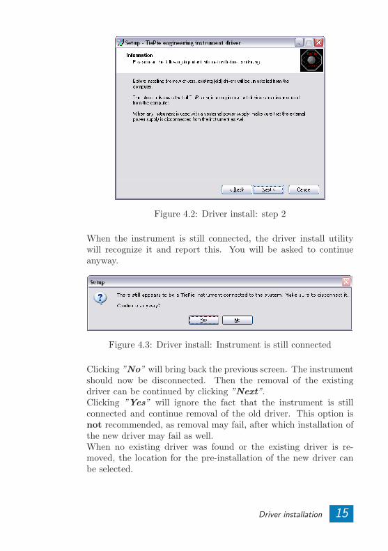
Figure 4.2: Driver install: step 2
When the instrument is still connected, the driver install utilitywill recognize it and report this. You will be asked to continueanyway.
Figure 4.3: Driver install: Instrument is still connected
Clicking ”No” will bring back the previous screen. The instrumentshould now be disconnected. Then the removal of the existingdriver can be continued by clicking ”Next”.Clicking ”Yes” will ignore the fact that the instrument is stillconnected and continue removal of the old driver. This option isnot recommended, as removal may fail, after which installation ofthe new driver may fail as well.When no existing driver was found or the existing driver is re-moved, the location for the pre-installation of the new driver canbe selected.
Driver installation 15
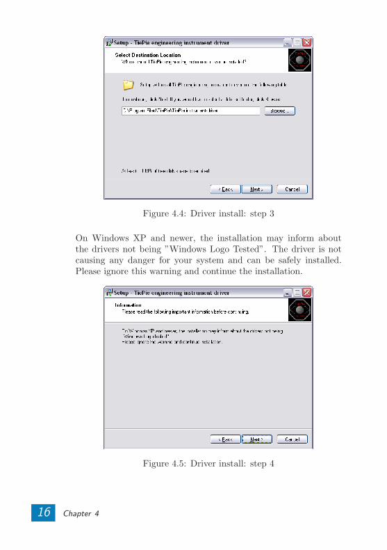
Figure 4.4: Driver install: step 3
On Windows XP and newer, the installation may inform aboutthe drivers not being ”Windows Logo Tested”. The driver is notcausing any danger for your system and can be safely installed.Please ignore this warning and continue the installation.
Figure 4.5: Driver install: step 4
16 Chapter 4
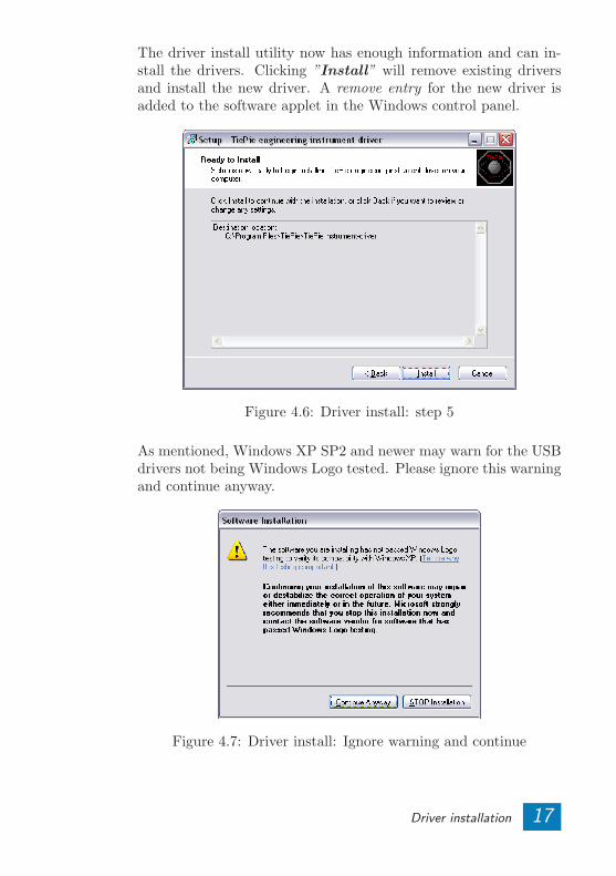
The driver install utility now has enough information and can in-stall the drivers. Clicking ”Install” will remove existing driversand install the new driver. A remove entry for the new driver isadded to the software applet in the Windows control panel.
Figure 4.6: Driver install: step 5
As mentioned, Windows XP SP2 and newer may warn for the USBdrivers not being Windows Logo tested. Please ignore this warningand continue anyway.
Figure 4.7: Driver install: Ignore warning and continue
Driver installation 17

Figure 4.8: Driver install: Finished
18 Chapter 4
Hardware installation 5
Drivers have to be installed before the Handyscope HS3 isconnected to the computer for the first time. See chapter 4for more information.
5.1 Power the instrument
The Handyscope HS3 is powered by the USB, no external powersupply is required. Only connect the Handyscope HS3 to a buspowered USB port, otherwise it may not get enough power to op-erate properly.
5.1.1 External power
In certain cases, it can be that the Handyscope HS3 cannot getenough power from the USB port.When a Handyscope HS3 is connected to a USB port, the hardwarewill be powered, resulting in an inrush current, which is higherthan the nominal current. After the inrush current, the currentwill stabilize at the nominal current.USB ports have a maximum limit for both the inrush current peakand the nominal current. When either of them is exceeded, theUSB port will be switched off. As a result, the connection to theHandyscope HS3 will be lost.Most USB ports can supply enough current for the HandyscopeHS3 to work without an external power supply, but this is notalways the case. Some (battery operated) portable computers or(bus powered) USB hubs do not supply enough current. The exactvalue at which the power is switched off, varies per USB controller,so it is possible that the Handyscope HS3 functions properly onone computer, but does not on another.In order to power the Handyscope HS3 externally, an externalpower input is provided for. It is located at the rear of the Handy-
Hardware installation 19
scope HS3. Refer to paragraph 7.1 for specifications of the externalpower intput.
5.2 Connect the instrument to the computer
After the new driver has been pre-installed (see chapter 4), theHandyscope HS3 can be connected to the computer. When theHandyscope HS3 is connected to a USB port of the computer,Windows will report new hardware. The Found New HardwareWizard will appear.Depending on the Windows version, the New Hardware Wizardwill show a number of screens in which it will ask for informationregarding the drivers of the newly found hardware. The appearanceof the dialogs will differ for each Windows version and might bedifferent on the computer where the Handyscope HS3 is installed.
The driver consists of two parts which are installed sepa-rately.
Once the first part is installed, the installation of the second partwill start automatically. Installation of the second part is identicalto the first part, therefore they are not described individually here.
20 Chapter 5

5.2.1 Found New Hardware Wizard
Figure 5.1: Hardware install: step 1
This window will only be shown in Windows XP SP2 or newer.No drivers for the Handyscope HS3 can be found on the WindowsUpdate Web site, so select ”No, not this time” and click ”Next”.
Figure 5.2: Hardware install: step 2
Hardware installation 21

Since the drivers are already pre-installed on the computer, Win-dows will be able to find them automatically. Select ”Install thesoftware automatically” and click ”Next”.
Figure 5.3: Hardware install: step 3
The New Hardware wizard will now copy the required files to theirdestination.
Figure 5.4: Hardware install: step 4
22 Chapter 5
The first part of the new driver is now installed. Click ”Finish”to close the wizard and start installation of the second part, whichfollows identical steps.Once the second part of the driver is installed. measurement soft-ware can be installed and the Handyscope HS3 can be used.
5.3 Plug into a different USB port
When the Handyscope HS3 is plugged into a different USB port,some Windows versions will treat the Handyscope HS3 as differenthardware and will ask to install the drivers again. This is controlledby Microsoft Windows and is not caused by TiePie engineering.
Hardware installation 23

24 Chapter 5
Front panel 6
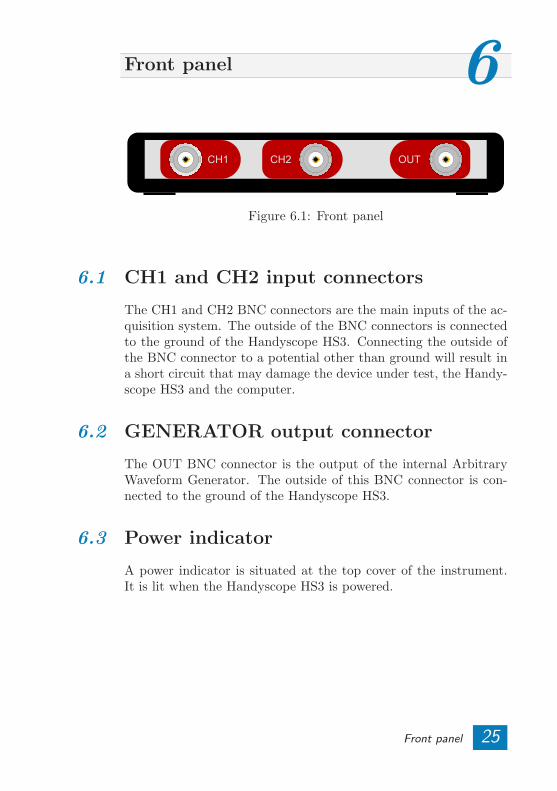
Figure 6.1: Front panel
6.1 CH1 and CH2 input connectors
The CH1 and CH2 BNC connectors are the main inputs of the ac-quisition system. The outside of the BNC connectors is connectedto the ground of the Handyscope HS3. Connecting the outside ofthe BNC connector to a potential other than ground will result ina short circuit that may damage the device under test, the Handy-scope HS3 and the computer.
6.2 GENERATOR output connector
The OUT BNC connector is the output of the internal ArbitraryWaveform Generator. The outside of this BNC connector is con-nected to the ground of the Handyscope HS3.
6.3 Power indicator
A power indicator is situated at the top cover of the instrument.It is lit when the Handyscope HS3 is powered.
Front panel 25

26 Chapter 6
Rear panel 7
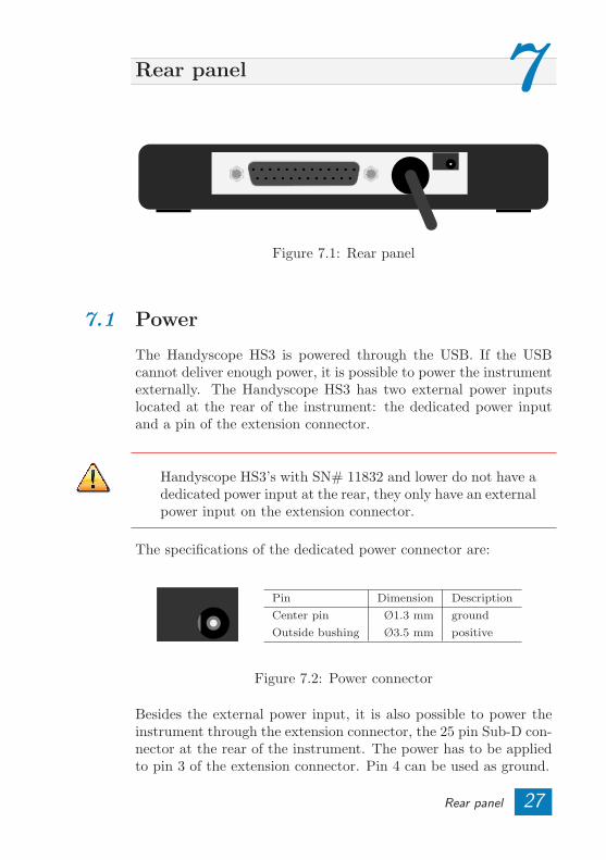
Figure 7.1: Rear panel
7.1 Power
The Handyscope HS3 is powered through the USB. If the USBcannot deliver enough power, it is possible to power the instrumentexternally. The Handyscope HS3 has two external power inputslocated at the rear of the instrument: the dedicated power inputand a pin of the extension connector.
Handyscope HS3’s with SN# 11832 and lower do not have adedicated power input at the rear, they only have an externalpower input on the extension connector.
The specifications of the dedicated power connector are:
Pin Dimension Description
Center pin Ø1.3 mm ground
Outside bushing Ø3.5 mm positive
Figure 7.2: Power connector
Besides the external power input, it is also possible to power theinstrument through the extension connector, the 25 pin Sub-D con-nector at the rear of the instrument. The power has to be appliedto pin 3 of the extension connector. Pin 4 can be used as ground.
Rear panel 27

The following minimum and maximum voltages apply to both powerinputs:
Minimum Maximum
SN# <12941 4.5 Volt DC 6 Volt DC
SN# >12941 4.5 Volt DC 12 Volt DC
Table 7.1: Maximum voltages
Note that the externally applied voltage should be higher than theUSB voltage to relieve the USB port.
7.1.1 USB power cable
The Handyscope HS3 is delivered with a special USB externalpower cable.
Figure 7.3: USB power cable
One end of this cable can be connected to a second USB port onthe computer, the other end can be plugged in the external powerinput at the rear of the instrument. The power for the instrumentwill be taken from two USB ports of the computer.
The outside of the external power connector is connected to+5 Volt. In order to avoid shortage, first connect the cableto the Handyscope HS3 and then to the USB port.
28 Chapter 7

7.1.2 Power adapter
In case a second USB port is not available, or the computer stillcan’t provide enough power for the instrument, an external poweradapter can be used. When using an external power adapter, makesure that:
• the polarity is set correctly• the voltage is set to a valid value for the instrument and
higher than the USB voltage• the adapter can supply enough current (preferably >1 A)• the plug has the correct dimensions for the external power
input of the instrument
7.2 USB
The Handyscope HS3 is equipped with a USB 2.0 High speed (480Mbit/sec) interface with a fixed cable with type A plug. It willalso work on a computer with a USB 1.1 interface, but will thenoperate at 12 Mbit/sec.
7.3 Extension Connector
Figure 7.4: Extension connector
To connect to the Handyscope HS3 a 25 pin female Sub-D connec-tor is available, containing the following signals:
Rear panel 29

Pin Description Pin Description
1 Ground 14 Ground
2 Reserved 15 Ground
3 External Power in DC 16 Reserved
4 Ground 17 Ground
5 +5V out, 10 mA max. 18 Reserved
6 Ext. sampling clock in (TTL) 19 Reserved
7 Ground 20 Reserved
8 Ext. trigger in (TTL) 21 Generator Ext Trig in (TTL)
9 Data OK out (TTL) 22 Ground
10 Ground 23 I2C SDA
11 Trigger out (TTL) 24 I2C SCL
12 Reserved 25 Ground
13 Ext. sampling clock out (TTL)
Table 7.2: Pin description Extension connector
All TTL signals are 3.3 Volt TTL signals which are 5 Volt tolerant,so they can be connected to 5 Volt TTL systems.For instruments with serial number 14266 and higher, pins 9, 11, 12,13 are open collector outputs. Connect a pull-up resistor of 1 kOhmto pin 5 when using one of these signals. For older instruments,the outputs are standard TTL outputs and no pull-up is required.
30 Chapter 7
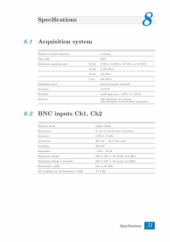
Specifications 88.1 Acquisition system
Number of input channels 2 analog
Ch1, Ch2 BNC
Maximum sampling rate 12 bit 5 MS/s, 10 MS/s, 25 MS/s or 50 MS/s
14 bit 3.125 MS/s
16 bit 195 kS/s
8 bit 100 MS/s
Sampling source internal quartz, external
Accuracy ±0.01%
Stability ±100 ppm over −40C to +85C
Memory 128 kSamples per channel(256 kSamples with disabled generator)
8.2 BNC inputs Ch1, Ch2
Measure mode Single ended
Resolution 8, 12, 14, 16 bit user selectable
Accuracy 0.2% ± 1 LSB
Sensitivity 200 mV .. 80 V full scale
Coupling AC/DC
Impedance 1 MΩ / 30 pF
Maximum voltage 200 V (DC + AC peak <10 kHz)
Maximum voltage 1:10 probe 600 V (DC + AC peak <10 kHz)
Bandwidth (-3dB) DC to 50 MHz
AC coupling cut off frequency (-3dB) ±1.5 Hz
Specifications 31
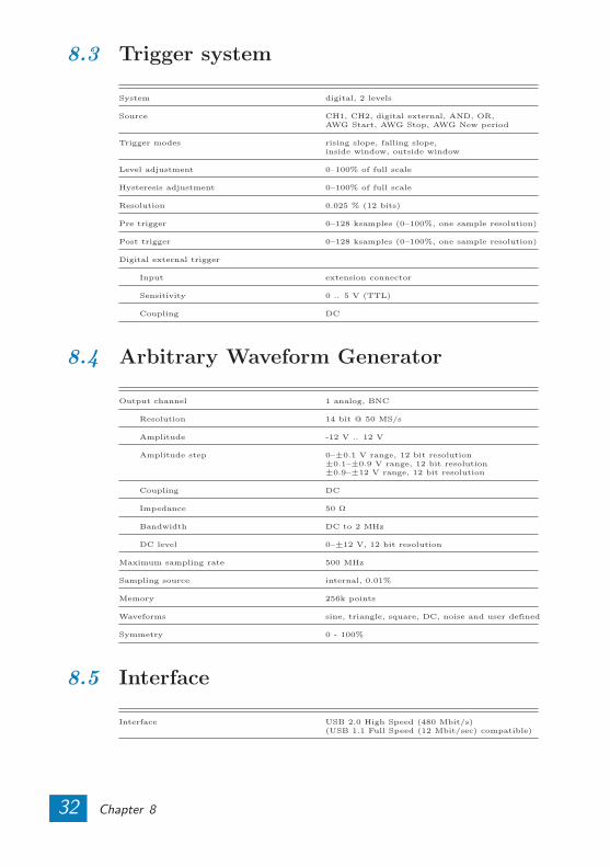
8.3 Trigger system
System digital, 2 levels
Source CH1, CH2, digital external, AND, OR,AWG Start, AWG Stop, AWG New period
Trigger modes rising slope, falling slope,inside window, outside window
Level adjustment 0–100% of full scale
Hysteresis adjustment 0–100% of full scale
Resolution 0.025 % (12 bits)
Pre trigger 0–128 ksamples (0–100%, one sample resolution)
Post trigger 0–128 ksamples (0–100%, one sample resolution)
Digital external trigger
Input extension connector
Sensitivity 0 .. 5 V (TTL)
Coupling DC
8.4 Arbitrary Waveform Generator
Output channel 1 analog, BNC
Resolution 14 bit @ 50 MS/s
Amplitude -12 V .. 12 V
Amplitude step 0–±0.1 V range, 12 bit resolution±0.1–±0.9 V range, 12 bit resolution±0.9–±12 V range, 12 bit resolution
Coupling DC
Impedance 50 Ω
Bandwidth DC to 2 MHz
DC level 0–±12 V, 12 bit resolution
Maximum sampling rate 500 MHz
Sampling source internal, 0.01%
Memory 256k points
Waveforms sine, triangle, square, DC, noise and user defined
Symmetry 0 - 100%
8.5 Interface
Interface USB 2.0 High Speed (480 Mbit/s)(USB 1.1 Full Speed (12 Mbit/sec) compatible)
32 Chapter 8

8.6 Power
Input from USB or external input
Consumption 500 mA max
8.7 Physical
Instrument height 25 mm / 1.0”
Instrument length 170 mm / 6.7”
Instrument width 140 mm / 5.2”
Weight 480 gram / 17 ounce
USB cord length 1.8 m / 70”
8.8 I/O connectors
Ch1–Ch2 BNC
Generator out BNC
Power 3.5 mm power socket
Extension connector Sub-D 25 pins female
8.9 System requirements
PC I/O connection USB 2.0 High Speed (480 Mbit/s)(USB 1.1 Full Speed (12 Mbit/sec) compatible)
Operating System Windows 98/ME/2000/XP/Vista-32
8.10 Operating environment
Ambient temperature 0 - 55C
Relative humidity 10 to 90% non condensing
8.11 Storage environment
Ambient temperature -20 - 70C
Relative humidity 5 to 95% non condensing
Specifications 33

8.12 Certifications and Compliances
CE mark compliancee Yes
RoHS Yes
8.13 Package
Instrument Handyscope HS3
Probes 2 x 1:1 / 1:10 switchable
Accessories PS2 power cable
Software Windows 98/2000/ME/XP/Vista-32
Drivers Windows 98/2000/ME/XP/Vista-32
Manual Instrument manual and software user’s manual
34 Chapter 8

If you have any suggestions and/or remarks regarding this applicationor the manual, please contact:
@@TiePie engineeringP.O. Box 2908600 AG SNEEKThe Netherlands
@ TiePie engineeringKoperslagersstraaat 378601 WL SNEEKThe Netherlands
Tel.: +31 515 415 416Fax: +31 515 418 819E-mail: [email protected]: www.tiepie.nl