Johnson & Wales UniversityScholarsArchive@JWUEngineering Studies Faculty Publications andCreative Works College of Engineering & Design

1995

Using MATLAB to Illustrate the 'Phenomenon ofAliasing'Sol Neeman, Ph.D.Johnson & Wales University - Providence, sneeman@jwu.edu

Follow this and additional works at: https://scholarsarchive.jwu.edu/engineering_fac

Part of the Computer Engineering Commons, Electrical and Computer Engineering Commons,Engineering Science and Materials Commons, Mechanical Engineering Commons, OperationsResearch, Systems Engineering and Industrial Engineering Commons, and the Other EngineeringCommons

This Conference Proceeding is brought to you for free and open access by the College of Engineering & Design at ScholarsArchive@JWU. It has beenaccepted for inclusion in Engineering Studies Faculty Publications and Creative Works by an authorized administrator of ScholarsArchive@JWU. Formore information, please contact jcastel@jwu.edu.

Repository CitationNeeman,, Sol Ph.D., "Using MATLAB to Illustrate the 'Phenomenon of Aliasing'" (1995). Engineering Studies Faculty Publications andCreative Works. 8.https://scholarsarchive.jwu.edu/engineering_fac/8

Session 1620

USING MATLAB TO ILLUSTRATE THE' PHENOMENON OF ALIASING

Sol Neeman Johnson and Wales University

Abstract

The phenomenon of aliasing is important when sam­pling analog signals. In cases where the signal is ban­dlimited, one can avoid aliasing by ensuring that the sampling rate is higher than the Nyquist rate . But in cases where the signal is not bandlimited , aliasing is un­avoidable if the signal is not filtered before it is sampled. It is then crucial to understand the phenomenon in order to estimate the distortion generated when the signal is reconstructed from its samples. Using the software pack­age MATLAB by MathWorks, Inc ., two examples are presented. The first is a pure sinusoid which is sampled at both higher and lower than the Nyquist rate , and the frequency spectrum of both sampled sinusoids are com­pared to illustrate the effect of aliasing. The second and more interesting case is a square wave which has an un­limited bandwidth. The square wave is a periodic wave that has Fourier expansion with odd harmonics only, the amplitudes of which drop as lin. A square wave is synthesized using MATLAB and its Fourier transform is presented graphically (The synthesized square wave inherently produces aliased components) . The odd har­monics and the aliased components seen on the graph are analyzed and compared to the predicted theoretical results . Graphs generated by MATLAB accompany the analysis for both signals.

Introduction

Physical signals in nature are continuous, both in time and in amplitude . On digital computers , they can be represented by finite sequences with finite precision. To do this , the signal has to be sampled and the ampli­tude of the samples be approximated by a finite number of bits (quantization of the signal) . Nyquist theorem states that the analog signal can be reconstructed from its samples, provided the sampling rate is greater than twice the highest frequency component in the analog signal. Thus if the highest frequency component is nn (called the Nyquist frequency), the sampling frequency, n., has to satisfy:

n. > 2 · nn (the frequency 2 . nn is called the Nyquist sampling

rate) If this condition is not satisfied, aliasing will occur , re­

sulting in distortion in the reconstructed signal from its samples. When signals are not bandlimited, anti aliasing filters can be used to minimize the effect by attenuating the undesired high frequency components. In addition, wideband additive noise may fill in the high frequency range and then be aliased into the lower frequency range. In order to evaluate quantitatively the distortion in the reconstructed signal , it is necessary to understand why the high frequency components are aliased into the lower range .

Why and how Aliasiug Occurs

To get an insight into this phenomenon, we analyze the Fourier transform of the sampled signal and compare it to the Fourier transform of the analog (continuous) signal[lj :

Let xa(t) represent an analog signal with the highest frequency component at nn, and set) represent a peri­odic impulse train , with a period T , that is:

set) = L 8(t - nT) n

where 8(t) is the unit impulse function. If Xa(t) is sampled at a period T , the sampled signal, xs (t) , can be represented as the product of the two, that is :

Xs(t) = xa(t) . set) = xa(t) . L 8(t - nT) n

Since multiplication in the time domain translates into convolution in the frequency domain , the relation­ship between the Fourier transforms of the three func­tions is given by:

x.un) = 2l7l'XaUn) * Sun)

1995 ASEE Annual Conference Proceedings

612

where n represents analog frequency. The Fourier transform of s(t), the periodic impulse train, is a pe­riodic impulse train in the frequency domain, that is:

sun) = :; L 8(n - k ;7r) = :; L 8(n - kn.) k k

Carrying out the convolution in the previous equation, results in:

This equation states that the Fourier transform of the sampled signal is a superposition of infinitely many shifted copies of Xaun), resulting in repeated copies of Xa un) in integer multiples of n., in both direc­tion of the frequency axis. If the sampling rate is not greater than twice the Nyquist frequency, the copies, when superimposed , will overlap and higher frequ~ncies will be aliased into the lower frequency range; therefore we would not be able to reconstruct the original signal from its samples by the use of a filter. On the other hand if the sampling rate is satisfied, no overlapping of the copies will happen and with the appropriate filter it is possible to reconstruct the original signal from its samples .

Fig. 1 represents the Fourier transform of xa(t) and x s (t) and the two cases described above.

~.\'.(jll l , \I

-IlN Us

¥t S(j\1)

t j t t ): U - 1 · 11., - II., lis :!. · lls

No ",Iia.s ill~ : 0 ,,; > 2· fiN

- fls

- Os -fix n,\' Po ...

Fig.1 Fourier Transform of an analog signal, xa(t) and its sampled form, x.(t).

Aliasing can also be demonstrated in a simpler way, when we analyze the relationship between the sampled

versions of a group of pure sinusoids[21. Consider the continuous sinusoid of frequency Wo :

x(t) = sin(wo' t)

When sampled at a sampling period T, the resulting sampled sequence is:

x(n) = sin(wo . n· T) for n=0,±1,±2, ...

Now consider the group of sinusoids of frequency w, where:

27rk w=wo+ T for k = 0, ±l, ±2, ...

When sampled at a sampling period T, any sinusoid:

y(t) = sin[(wo + 2;k) . tj

from this group , will result in a sequence which is identical to the sampled sequence of frequency woo To see that, we observe:

y(n) = sin[(wo + 2;k) . nT] = sin[(wo . nT + 27rkn)]

= sin[wo . nT]

Thus x(t) and any ofthe sinusoids represented by y(t) , cannot be distinguished when sampled at a sampling period T. Note that Wo is considered in tandem with -wo°

Bin# and Actual Frequency Relationship in FFT Computation

When a sampled signal, x$(t) is represented by a . sequence x(n), the Fourier transform of the sequence, X(eiw ), is a frequency scaled version of x.(jn) with the scaling w = nT. Thus the analog frequency n = n. (where n .. = 27r/T ), is normalized to w = 27r. The FFT of a sequence of length N, produces N points (re­ferred to as bin # 's). In MATLAB, the first N/2 + 1 points correspond to the frequency range DC to 1./2 (Nyquist frequency) . The rest of the points correspond to negative frequencies (which will be truncated in . the following examples).

Thus, to translate the values of the bin #'s to the actual frequency f , we use the equation:

~i 1995 ASEE Annual Conference Proceedings 1",IIoO\O'l'

613

•

f = (bin# -1)· fs/N

Graphing FFT Values Versus the Actual Frequency , in Hz[3,41

To graph the FFT values Of a signal versus the actual frequency in Hz rather than versus the bin #, we have to generate a frequency vector of length N /2 + 1, evenly spaced, which represents the frequency range: DC to fs/2 . For example , let X(n) represent N points FFT with N even and a sampling frequency fs ; In MATLAB, we can produce a frequency vector Hz via:

Hz = Us/2) * (0: N/2)/(N/2);

Since X (n) is of length N and we need only the first N /2 + 1 elements, we have to truncate the portion that corresponds to negative frequencies. This is done via:

X(N/2 +2 : N) = [];

Then we can plot IX (n) I versus Hz.

Aliasing When Undel'sampling a pure sinusoid

To illustrate aliasing when a pure sinusoid is undersam­pled , we use MATLAB to synthesize a sinusoid of fre­quency 550Hz, then represent it by two sequences:

l)A sequence corresponding to a sampling frequency of f s = 2, OOOH::, thus satisfying the sampling rate in Nyquist. theorem.

2)A sequence corresponding to a sampling frequency of Is = 1, OOOH z, a sampling rate lower than the Nyquist rate.

Then we compute the FFT ofthese sequences and plot the results. Clearly, in the second case the frequency of 550H z will be aliased into the range 0 - 500Hz (Note that when sampling at a rate of fs , the FFT values will correspond to the range of frequencies: DC to fs/2). Thus the FFT values for the sequence representing a sampling rate of 1000Hz will correspond to the fre­quency range DC to 500 Hz and the FFT values for the sequence representing a sampling rate of 2000Hz will correspond to the frequency range DC to 1000Hz.

We will define two time indices, t1 and t2, of 1024 points each and two frequency vectors H zl and H z2:

tl runs from 0.00 to 0.5115 seconds, in steps of .5ms, equivalent to a sampling rate of 2, OOOH z.

t2 runs from 0.00 to 1.023 seconds, in steps of Ims, equivalent to a sampling rate of l, OOOH z .

Hz 1, the first frequency vector, runs from DC to 1, OOOH z.

H z2, the second frequency vector, runs from DC to 500Hz.

The next lines are the commands in MA TLAB needed to produce both sequences, compute their FFT and plot the results [31:

t1=0:.0005:.5115; Hz 1 =(2000/2)*(0: 1024/2) / (lO24/2); xl=sin(2*pi*550*tl ); Xl=abs(fft(xl »; Xl(514:1024)=[ ]; subplot(211) ; plot( tl( 1 :64),xl(1 :64)); subplot(212); plot(Hz 1 ,Xl); (Fig. 2 shows MATLAB plots for xl and Xl)

t2=0:.00l:1.023; Hz2=( 1 000/2)*(0: 1024/2) / (lO24/2); x2=sin( 2*pi * 550*t2); X2=abs(fft(x2)); X2(514:1024)=[ ]; subplot(21l); plot( t2(1 :256),x2( 1 :256)); subplot(212); plot(Hz2,X2); (Fig . 3 shows MATLAB plots for x2 and X2)

-~-- - .----_. ,---_. __ . . _.- .,

11 . 0.5

f\ h ~ t1 I .s 0 x

-0.5

-1 o

400

!;300

hoo •

100

V ~ V \I

0.005 0.01

I

V ~ V \ V ~ -

0.015 0.02 0.025 0.03 0.035 l(Ms)

00 100 200 300 400 500 600 700 800 900 1000 frequency(Hz)

Fig.2 550Hz sine wave sampled at fs = 2, OOOH z and its FFT.

•

,".0 •• "". l. ~~ . . 1995 ASEE Annual Conference Proceedings \ l

• ... , .. / .... c; .. ou" ..

614

.......... ____ 111111111111111111 11 111 11111 ___ III"IIIIIiIiIJJIIII'1 _____ ... __ "",IIWIII!!._.J,,_""

i

1 ---,----.. . , -. --- ., ._- -~,-------;-,--~

<? ~ ~Nl~ ~ o 0.01 0.02 0.03 0.04 0_05 0.06 0_07

t(Ms)

500 r--- · ·-~---- ~-- - , - -. ---~- -~----~ - --- -.. ,--- -

400

~300 ~ !"200 •

100

°O~~~~--~-~~------~~~~~~~~ 50 100 150 200 250 300 350 400 450 500

frequency(Hz)

Fig.3 550Hz sine wave sampled at i. and its FFT.

1, OOOH z

Notice that Xl in the upper graph of Fig. 2 correctly represents the frequency component of 550H z. The plot of X2, on the other hand , shows that the frequency of 550H:: is aliased into the frequency 450H z. This is in ac­cordance with the previous analysis we have since when the spectrum of x(t), the continuous signal, is copied (in integer multiples of 1000Hz, on both sides of the fre­quency axis), the frequency 550H z will be aliased into the frequency 450Hz.

Aliasing When Representing a Square Wave By a Discrete Sequence

As was mentioned before, when an analog signal con­tains frequency components higher than 0,s /2, these components will be aliased into the range DC to 0,./2. A square wave is an interesting example to illustrate this effect . Consider a periodic square wave with period T = 211" /wo whose Fourier series is given by:

X(t) = ± f sin(2k + l)wot 11" k=O (2k + 1)

The Fourier expansion contains only odd harmonics, the amplitude of which drop as l/n (where n=harmonic #) and is infinite. This means that inherently any rep­resentation of a square wave by a discrete sequence will result in aliasing.

To illustrate this using MATLAB, we synthesize a square wave, compute and plot the magnitude of its FFT and compare the results to the predicted aliased components. We will synthesize a 30Hz square wave

with 50% duty cycle, consisting of 1024 points, sampled at a frequency of 1000Hz. The following are the com­mands inMATLAB needed to synthesize a square wave, compute its FFT and plot the results:

x=square(2*pi*30*t2,50); X=abs(fft(x)); X(514:1024)=[ ]; plot(Hz2,X); where t2 and Hz2 are those generated in the previous

example and "square" is a command from the Signal Processing Toolbox .

Fig 4 shows the graphs generated by MATLAB .

600

500

400

E >< 300 !" .

200

100

Fig. 4 FFT of a 30H z square wave .

First we will analyze the predicted aliasing effect. The first harmonic of the square wave is 30Hz , the

2nd is 90Hz, the 3rd 150Hz, etc. Since the sampling rate is is = 1000Hz, we should expect that all the har­monics above i./2 = 500Hz will be aliased into the range DC to 500H z.

The following is a list of the odd harmonics up to the 35th, the corresponding frequencies and for the frequen­cies above 500H z , the aliased frequency :

.~*: 1995 ASEE Annual Conference Proceedings \, .l ""'IfGt.o-l'

615

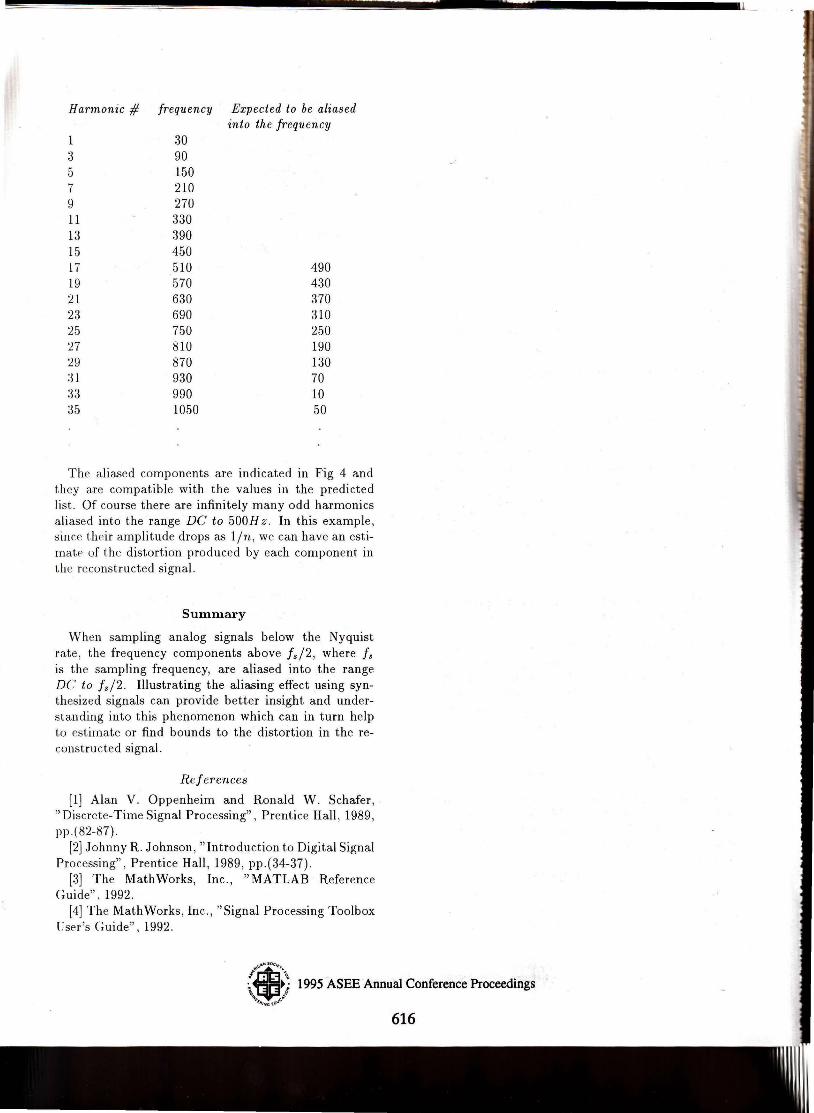
Harmonic # frequency Expected to be aliased into the frequency

1 30 3 90 5 150 7 210 9 270 11 330 13 390 15 450 17 5lO 490 19 570 430 21 630 370 23 690 3lO 25 750 250 27 810 190 29 870 130 :31 930 70 33 990 10 ;~5 1050 50

The aliased components are indicated in Fig 4 and they are compatible with the values in the predicted list. Of course there are infinitely many odd harmonics aliased into the range DC to 500Hz. In this example, since their amplitude drops as lin , we can have an esti­mate of the distortion produced by each component in the reconstructed signal.

Summary

When sampling analog signals below the Nyquist rate, the frequency components above fs/2, where fs is the sampling frequency, are aliased into the range DC to f./2 . Illustrating the aliasing effect using syn­thesized signals can provide better insight and under­standing into this phenomenon which can in turn help to estimate or find bounds to the distortion in the re­constructed signal.

References

[1) Alan V. Oppenheim and Ronald W . Schafer , " Discrete-Time Signal Processing" , Prentice Hall , 1989 , pp .( 82-87).

[2) Johnny R. Johnson, " Introduction to Digital Signal Processing" , Prentice Hall , 1989 , pp .(34-37) .

[3) The MathWorks, Inc., "MATLAB Reference Guide", 1992 .

[4) The Math Works, Inc. , " Signal Processing Toolbox User's Guide" , 1992.

(~; 1995 ASEE Annual Conference Proceedings '1tINGtO'o)

616

1111