mulit phase 2

STAR-CCM+ User Guide Capillary Effects Tutorial 4040

Version 4.04.011

The velocity vector plot shows high air velocities close to the free surface.This is a numerical inaccuracy known as parasitic currents. These currentsarise because the surface tension and pressure forces are much larger thanall other terms in the momentum equations, and their balance on anirregular grid is difficult to achieve numerically due to the discontinuousvariation of pressure across the free surface and a large discretization errorassociated with it. Parasitic currents become appreciable when the problemsize is small and fluid velocity and viscosity are low. For flows wherediffusion and convection forces are of a similar magnitude to surfacetension forces, these problems are not so pronounced. Since artificialvelocities are generated only within the air, their effect on the liquid flow(which is usually what we are trying to predict) is small.

• Save the simulation.

Changing the Contact Angle

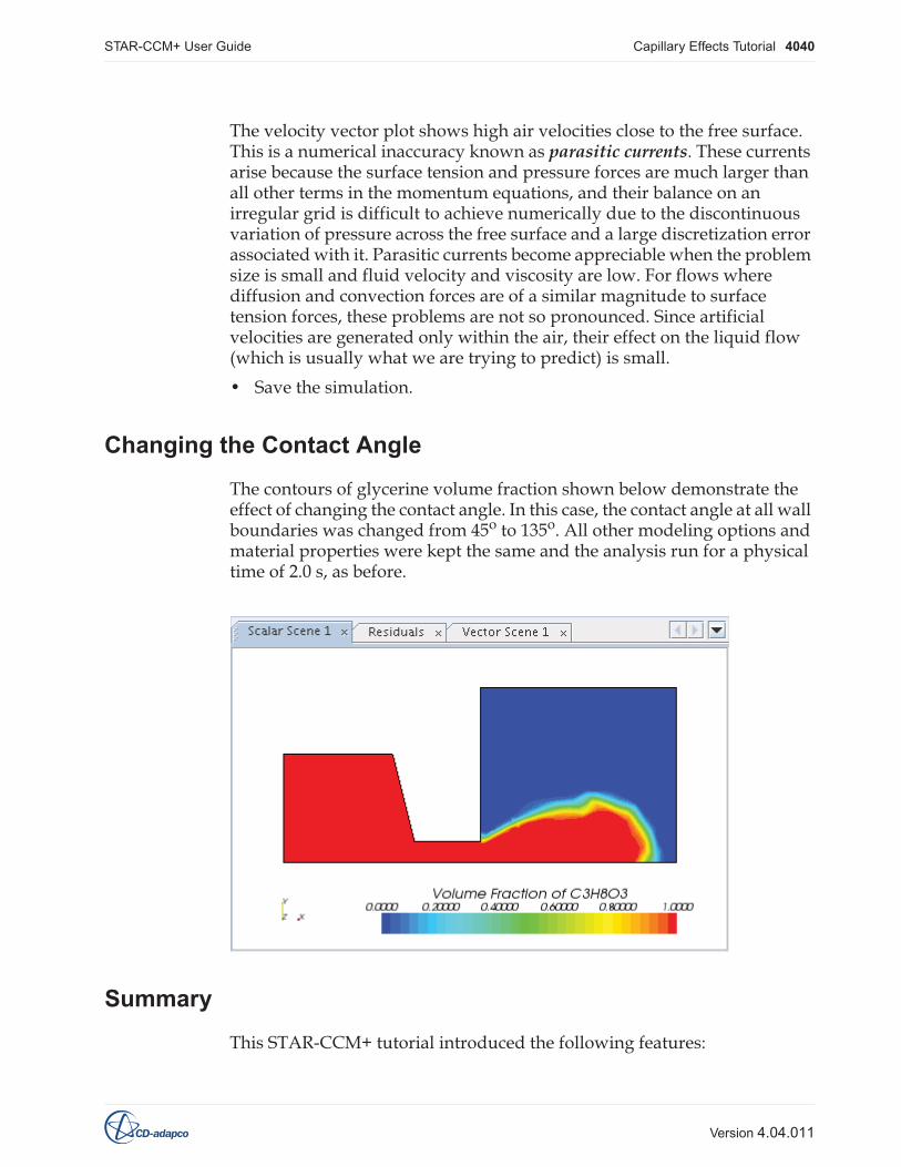
The contours of glycerine volume fraction shown below demonstrate theeffect of changing the contact angle. In this case, the contact angle at all wallboundaries was changed from 45o to 135o. All other modeling options andmaterial properties were kept the same and the analysis run for a physicaltime of 2.0 s, as before.

Summary

This STAR-CCM+ tutorial introduced the following features:

STAR-CCM+ User Guide 4042

Version 4.04.011

Cavitation Tutorial

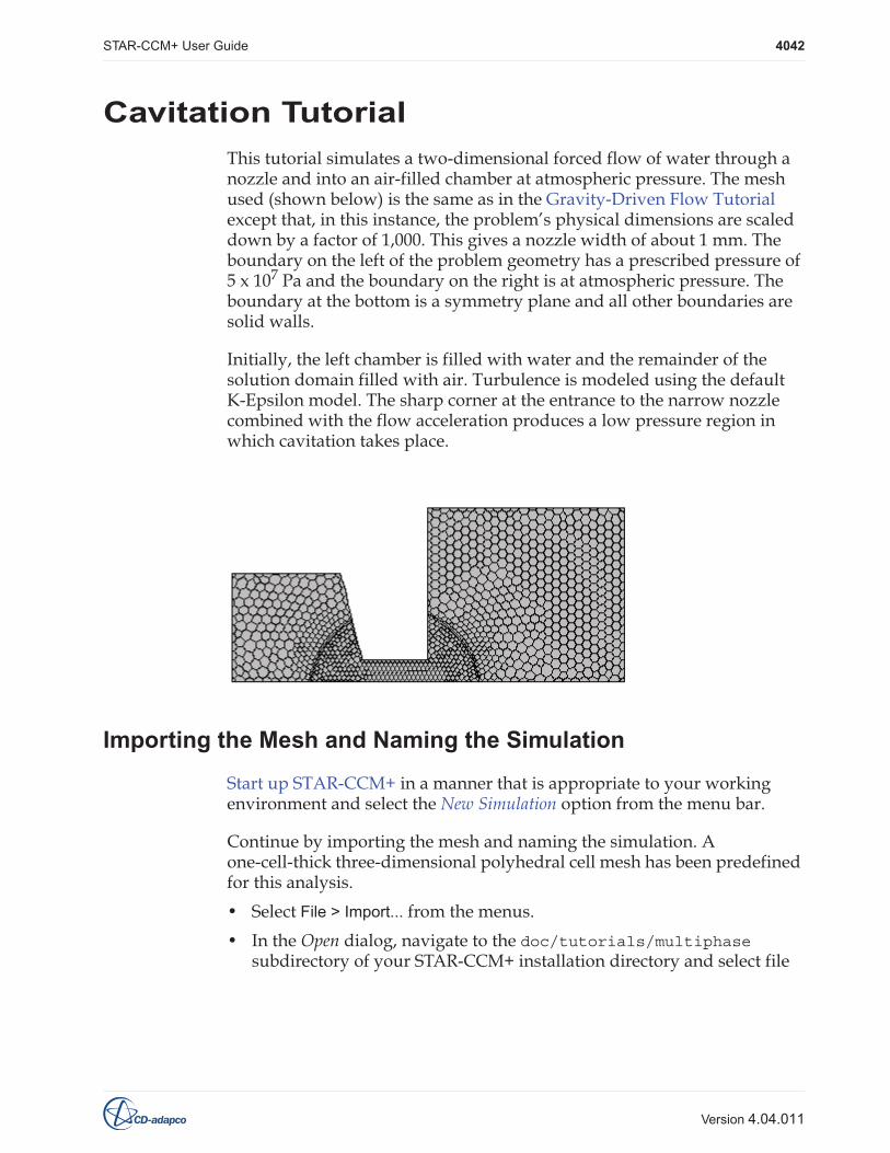
This tutorial simulates a two-dimensional forced flow of water through anozzle and into an air-filled chamber at atmospheric pressure. The meshused (shown below) is the same as in the Gravity-Driven Flow Tutorialexcept that, in this instance, the problem’s physical dimensions are scaleddown by a factor of 1,000. This gives a nozzle width of about 1 mm. Theboundary on the left of the problem geometry has a prescribed pressure of5 x 107 Pa and the boundary on the right is at atmospheric pressure. Theboundary at the bottom is a symmetry plane and all other boundaries aresolid walls.

Initially, the left chamber is filled with water and the remainder of thesolution domain filled with air. Turbulence is modeled using the defaultK-Epsilon model. The sharp corner at the entrance to the narrow nozzlecombined with the flow acceleration produces a low pressure region inwhich cavitation takes place.

Importing the Mesh and Naming the Simulation

Start up STAR-CCM+ in a manner that is appropriate to your workingenvironment and select the New Simulation option from the menu bar.

Continue by importing the mesh and naming the simulation. Aone-cell-thick three-dimensional polyhedral cell mesh has been predefinedfor this analysis.

• Select File > Import... from the menus.

• In the Open dialog, navigate to the doc/tutorials/multiphasesubdirectory of your STAR-CCM+ installation directory and select file

STAR-CCM+ User Guide Cavitation Tutorial 4044

Version 4.04.011

• The grid must be aligned with the X-Y plane.

• The grid must have a boundary plane at the Z = 0 location.

The mesh imported for this tutorial was built with these requirements inmind. Were the grid not to conform to the above conditions, it would havebeen necessary to realign the region using the mesh transformation androtation capabilities in STAR-CCM+.

• Select Mesh > Convert to 2D...

• In the Convert Regions to 2D dialog that appears, make sure thecheckbox of the Delete 3D regions after conversion option is ticked, andclick OK.

Once you click OK, the mesh conversion will take place and the newtwo-dimensional mesh will be shown, viewed from the z-direction, in theGeometry Scene 1 display. The mouse rotation option is suppressed fortwo-dimensional scenes.

• Right-click the Physics 1 continuum node and select Delete.

• Click Yes in the confirmation dialog.

Scaling the Mesh

The original mesh was not built to the correct scale and therefore requiresscaling down by a factor of 1000.

• Select Mesh > Scale Mesh... from the menu bar.


Version 4.04.011

Setting Material Properties

• In the cavitation window, open the Continua node.

The color of the Injector node has turned from gray to blue to indicate thatmodels have been activated.

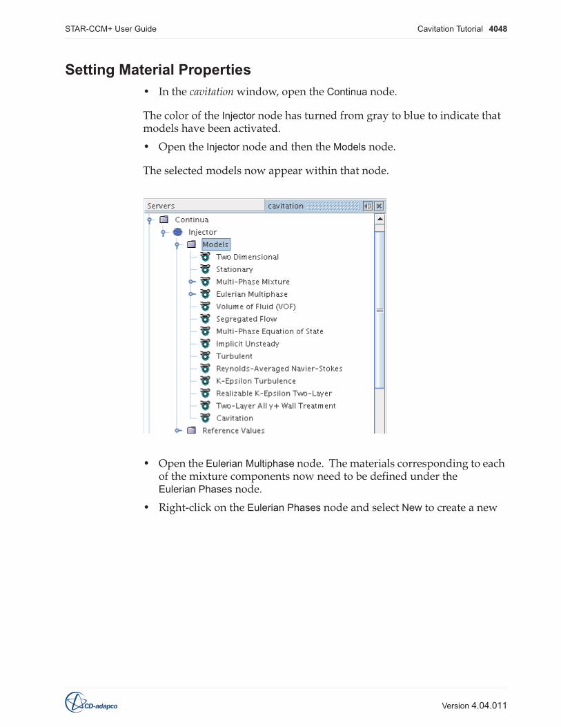
• Open the Injector node and then the Models node.

The selected models now appear within that node.

• Open the Eulerian Multiphase node. The materials corresponding to eachof the mixture components now need to be defined under theEulerian Phases node.

• Right-click on the Eulerian Phases node and select New to create a new


Version 4.04.011

The phase model objects should appear as shown in the followingscreenshot.

The default material properties for the three phases are suitable for thisproblem so we will now proceed to Defining Cavitation Model Parameters.


Defining Cavitation Model Parameters

In cavitation problems, it is necessary to specify which liquid phase iscavitating and which gas phase is the product of cavitation.


Version 4.04.011

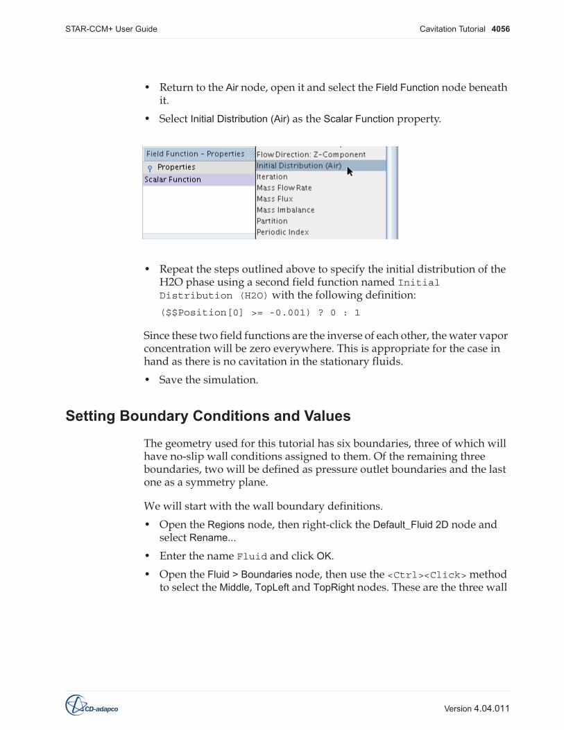
• Return to the Air node, open it and select the Field Function node beneathit.

• Select Initial Distribution (Air) as the Scalar Function property.

• Repeat the steps outlined above to specify the initial distribution of theH2O phase using a second field function named InitialDistribution (H2O) with the following definition:

($$Position[0] >= -0.001) ? 0 : 1

Since these two field functions are the inverse of each other, the water vaporconcentration will be zero everywhere. This is appropriate for the case inhand as there is no cavitation in the stationary fluids.


Setting Boundary Conditions and Values

The geometry used for this tutorial has six boundaries, three of which willhave no-slip wall conditions assigned to them. Of the remaining threeboundaries, two will be defined as pressure outlet boundaries and the lastone as a symmetry plane.

We will start with the wall boundary definitions.

• Open the Regions node, then right-click the Default_Fluid 2D node andselect Rename...

• Enter the name Fluid and click OK.

• Open the Fluid > Boundaries node, then use the <Ctrl><Click> methodto select the Middle, TopLeft and TopRight nodes. These are the three wall


Version 4.04.011

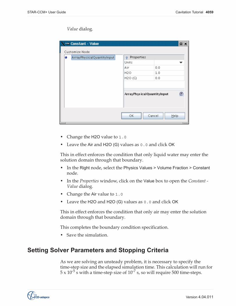
Value dialog.

• Change the H2O value to 1.0

• Leave the Air and H2O (G) values as 0.0 and click OK

This in effect enforces the condition that only liquid water may enter thesolution domain through that boundary.

• In the Right node, select the Physics Values > Volume Fraction > Constantnode.

• In the Properties window, click on the Value box to open the Constant -Value dialog.

• Change the Air value to 1.0

• Leave the H2O and H2O (G) values as 0.0 and click OK

This in effect enforces the condition that only air may enter the solutiondomain through that boundary.

This completes the boundary condition specification.


Setting Solver Parameters and Stopping Criteria

As we are solving an unsteady problem, it is necessary to specify thetime-step size and the elapsed simulation time. This calculation will run for5 x 10-5 s with a time-step size of 10-7 s, so will require 500 time-steps.


Version 4.04.011

Visualizing and Initializing the Solution

We will view the distributions of the three phases throughout the run bycreating a new scalar scene.

• Right-click on the Scenes node and then select New Scene > Scalar.

The Scalar Scene 1 display will appear.


Version 4.04.011

As expected, at the start of the run the left chamber is entirely filled withwater. Changing the scalar function to Volume Fraction of Air will show thatthe right chamber and the connecting channel are entirely filled with air. Asmall region in which both fluids are apparently present is visible at theinterface between the two fluids, but this effect is simply due to thecoarseness of the mesh.


Running the Simulation

• To run the simulation, click on the (Run) button in the top toolbar. Ifyou do not see this button, use the Solution > Run menu item instead.

The Residuals display will be created automatically and will show theprogress being made by the solver.

The run progress can be observed by selecting the Scalar Scene 1 tab at thetop of the Graphics window. Examine the distributions of each of the threephases by changing the scalar function regularly.

During the run it is possible to stop the process by clicking the (Stop)button in the toolbar. If you do halt the simulation, it can be continued againlater by clicking the (Run) button. If left alone, the simulation willcontinue until all 500 time-steps are complete. Note that the numbers


Version 4.04.011

To a reasonable approximation, the blue and turquoise areas arepredominantly occupied by air, the green areas predominantly by liquidwater and the yellow, orange and red areas predominantly by water vapor.

Manipulating the results in this way provides a qualitative visual estimateof the spatial extent of each phase. However, the resulting plots are prone toinaccuracies in those places where air and water vapor occur together andalso where the liquid water volume fraction is only slightly greater than thewater vapor volume fraction. In a case such as this, the latter leads to anoverprediction of the size of the region of high water vapor concentration.

To display velocity vectors:

• Right-click on the Scenes node and select New Scene > Vector

The vector scene will appear in the Graphics window.


Summary

This STAR-CCM+ tutorial introduced the following features:

• Importing a mesh and naming the simulation.

STAR-CCM+ User Guide 4069

Version 4.04.011

Particle-Laden Flow Tutorial

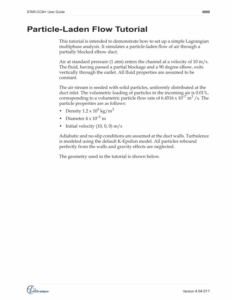
This tutorial is intended to demonstrate how to set up a simple Lagrangianmultiphase analysis. It simulates a particle-laden flow of air through apartially blocked elbow duct.

Air at standard pressure (1 atm) enters the channel at a velocity of 10 m/s.The fluid, having passed a partial blockage and a 90 degree elbow, exitsvertically through the outlet. All fluid properties are assumed to beconstant.

The air stream is seeded with solid particles, uniformly distributed at theduct inlet. The volumetric loading of particles in the incoming air is 0.01%,corresponding to a volumetric particle flow rate of 6.4516 x 10–7 m3 /s. Theparticle properties are as follows:

• Density 1.2 x 103 kg/m3

• Diameter 4 x 10–5 m

• Initial velocity (10, 0, 0) m/s

Adiabatic and no-slip conditions are assumed at the duct walls. Turbulenceis modeled using the default K-Epsilon model. All particles reboundperfectly from the walls and gravity effects are neglected.

The geometry used in the tutorial is shown below.

STAR-CCM+ User Guide Particle-Laden Flow Tutorial 4071

Version 4.04.011

STAR-CCM+ installation directory and select file elbow.ccmg.

• Click the Open button to start the import. The Import Mesh Optionsdialog will appear. Select the following options:

• Run mesh diagnostics after import

• Open geometry scene after import

• Ensure that the Don’t show this dialog during import option is not selectedand then click OK.

STAR-CCM+ will provide feedback on the import process, which will takea few seconds, in the Output window. One mesh region named Default_Fluidwill be created in the Regions node representing the grid domain. Ageometry scene will be created in the Graphics window.

Save the new simulation to disk under file name obstructedElbow.sim.

Visualizing the Imported Geometry

Examine the Geometry Scene 1 display in the Graphics window. To view thegeometry more clearly, change the viewing direction.

• Point anywhere in the Geometry Scene 1 display, hold down the leftmouse button and begin moving the mouse; this action rotates thevisualized parts.


Version 4.04.011

Geometry 1 node.

• In the Properties window, change the Opacity property to 0.5.

The obstruction in the elbow geometry is now clearly visible.


Setting up the Models

Models define the primary variables of the simulation, including pressure,temperature, velocity, and what mathematical formulation will be used togenerate the solution. In this example, the flow is turbulent andincompressible. The Segregated Flow model will be used together with the


Version 4.04.011

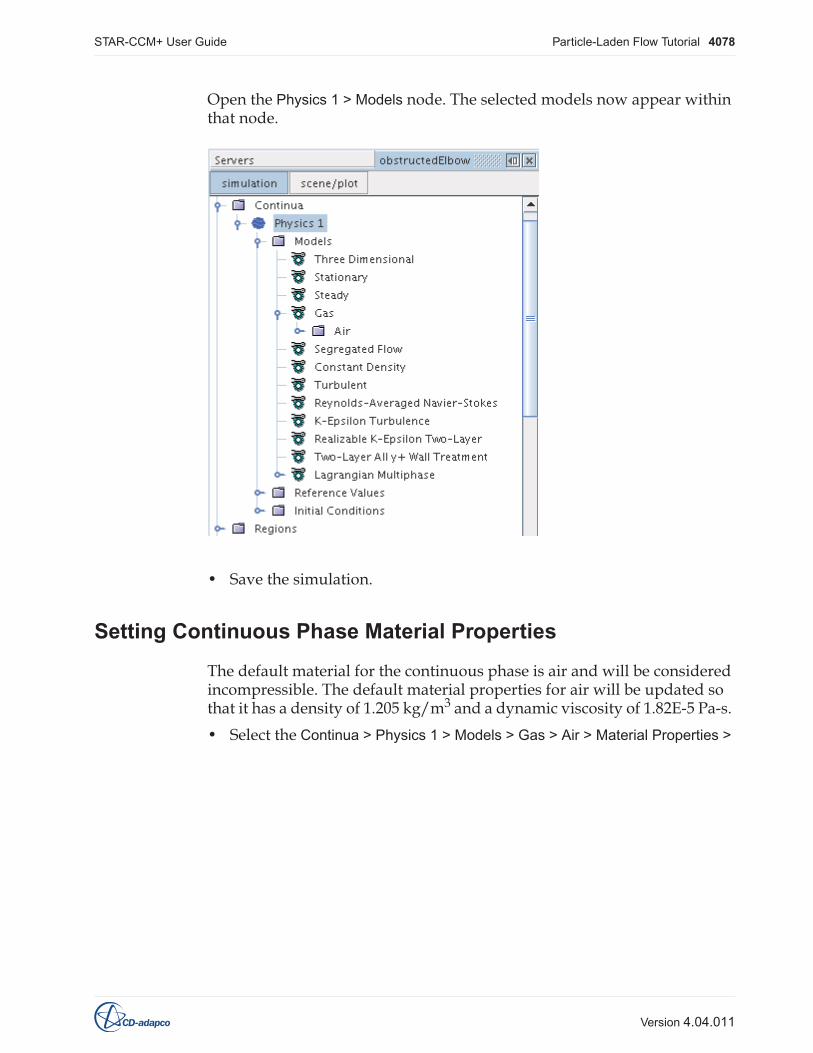
Open the Physics 1 > Models node. The selected models now appear withinthat node.


Setting Continuous Phase Material Properties

The default material for the continuous phase is air and will be consideredincompressible. The default material properties for air will be updated sothat it has a density of 1.205 kg/m3 and a dynamic viscosity of 1.82E-5 Pa-s.

• Select the Continua > Physics 1 > Models > Gas > Air > Material Properties >


Version 4.04.011

Setting Lagrangian Phase Model Properties

Properties for the Lagrangian Phase models may now be set.

• In the Continua > Physics 1 > Models > Lagrangian Multiphase >Lagrangian Phases > Phase 1 node, open the Models > Solid > Al >Material Properties > Density node.

• Select the Constant node and set the Value to 1200 kg/m3 in theProperties window.

• Select the Phase 1 > Models > Drag Force > Drag Coefficient node


Version 4.04.011

Phases > Phase 1 node, select the Boundary Conditions > Wall node.

• In the Properties window set the Mode property to Rebound.

• Open the Boundary Conditions > Wall node and select theNormal Restitution Coefficient > Constant and theTangential Restitution Coefficient > Constant subnodes in turn.

• Check the values for these coefficients in the Properties window. Theyshould both be set to 1 representing a perfect elastic rebound.


Setting Continuous Phase Boundary Conditions and Values

The default boundary conditions for the outlet and wall boundaries aresuitable for this analysis. The boundary conditions at the inlet, a fixed


Version 4.04.011

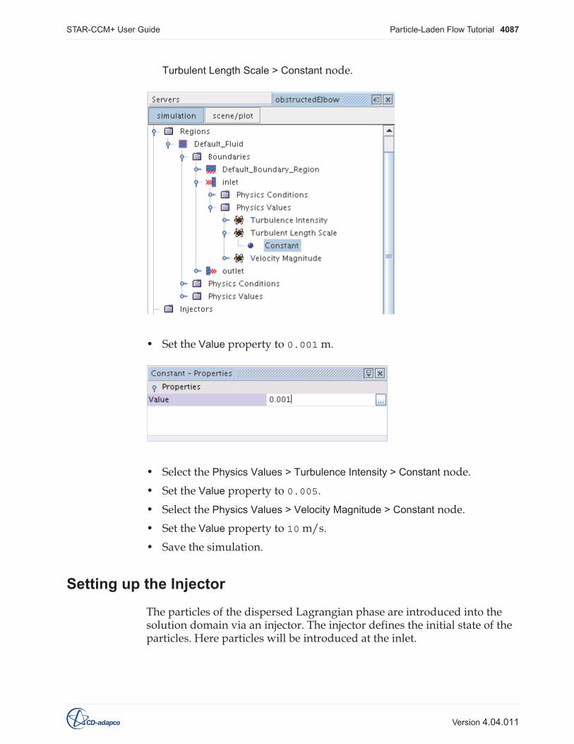
Turbulent Length Scale > Constant node.

• Set the Value property to 0.001 m.

• Select the Physics Values > Turbulence Intensity > Constant node.

• Set the Value property to 0.005.

• Select the Physics Values > Velocity Magnitude > Constant node.

• Set the Value property to 10 m/s.


Setting up the Injector

The particles of the dispersed Lagrangian phase are introduced into thesolution domain via an injector. The injector defines the initial state of theparticles. Here particles will be introduced at the inlet.


Version 4.04.011

Total.

This signifies that the volume flow rate applies to the whole injector, ratherthan per injection point.

• Select the Velocity Specification node and change the Method toMagnitude + Direction in the Properties window.

• Within the same Injector 1 node, select the Values > Volume Flow Rate >Constant node.

• In the Properties window set the Value property to 6.4516E-7 m3/s.

• Select the Values > Particle Diameter > Constant node and in the Propertieswindow set the Value to 4.0E-5 m.

• Select the Values > Velocity Magnitude node and in the Properties windowset the Value to 10 m/s.


Setting Solver Parameters and Stopping Criteria

Solver controls will be adjusted next. The maximum residence time for theLagrangian steady solver is set so that any particles that enter stagnant orrecirculating regions are not tracked indefinitely. In steady-statecalculations a particle is no longer tracked when its residence time reachesthis maximum.


Version 4.04.011

in the Properties window check that the Minimum Value is 1.0E-4.


Visualizing the Solution

We will view the velocity vectors on a cross-section through the fluid regionas the solution develops. Start by creating a new vector scene.

• Right-click the Scenes node, and select New Scene > Vector.

The Vector Scene 1 display will appear. Next a new plane section part will becreated for display.

• Right-click the Derived Parts node, and select New Part > Section > Plane....


Version 4.04.011

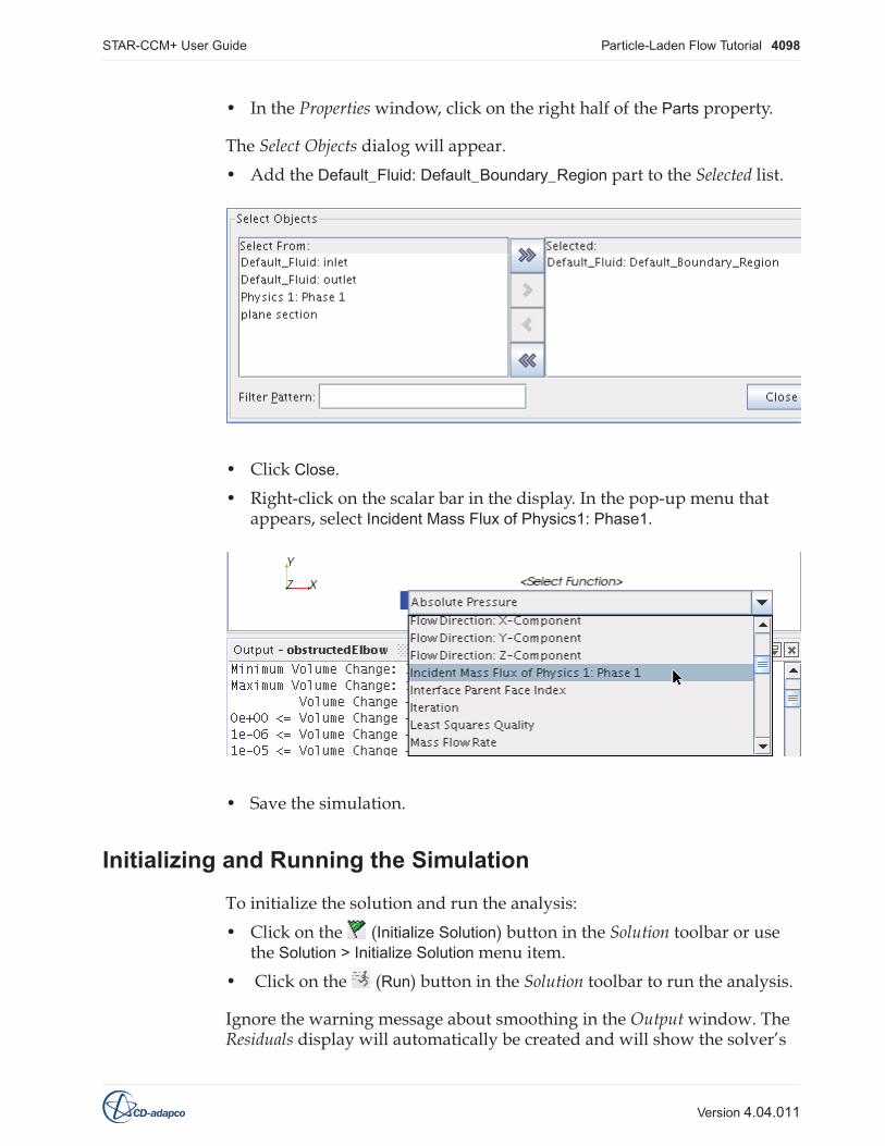
• In the Properties window, click on the right half of the Parts property.

The Select Objects dialog will appear.

• Add the Default_Fluid: Default_Boundary_Region part to the Selected list.

• Click Close.

• Right-click on the scalar bar in the display. In the pop-up menu thatappears, select Incident Mass Flux of Physics1: Phase1.


Initializing and Running the Simulation

To initialize the solution and run the analysis:

• Click on the (Initialize Solution) button in the Solution toolbar or usethe Solution > Initialize Solution menu item.

• Click on the (Run) button in the Solution toolbar to run the analysis.

Ignore the warning message about smoothing in the Output window. TheResiduals display will automatically be created and will show the solver’s


Version 4.04.011

Use the mouse controls to adjust the view approximately as shown below.

It can be seen that the particle impacts are concentrated on the outer radiusof the bend. In a realistic modeling exercise, a considerably larger numberof particles tracks would be needed to increase confidence in the results.

Displaying Particle Tracks

The particle tracks recorded by the Track File model will now be displayed.Start by creating a new track file.

mulit phase 2

Documents

pressure forces

summarythis starccm

atmospheric pressure

prescribed pressure

free surface

boundary plane

anirregular grid

flow acceleration