mtac tr09-01
TRANSCRIPT
MTAC Publication TR09-01 ISWS CR 2009-06
Spatial Variability of Arsenic in Groundwater
Thomas R. Holm and Steven D. Wilson
Center for Groundwater Science
Illinois State Water Survey
Illinois State Water Survey Institute of Natural Resource Sustainability University of Illinois at Urbana-Champaign
Disclaimer
This material is based upon work supported by the Midwest Technology Assistance Center for Small Public Water Systems (MTAC). MTAC was established October 1, 1998 to provide assistance to small public water systems throughout the Midwest via funding from the United States Environmental Protection Agency (USEPA) under section 1420(f) of the 1996 amendments to the Safe Drinking Water Act. MTAC is funded by the USEPA under Grant No. X83259101. Any opinions, findings, and conclusions or recommendations expressed in this publication are those of the author(s) and do not necessarily reflect the views of the USEPA or MTAC.
SPATIAL VARIABILITY OF ARSENIC IN GROUNDWATER
Thomas R. Holm and Steven D. Wilson
Center for Groundwater Science Illinois State Water Survey
April 2009

iii
Table of Contents
Page Abstract ............................................................................................................................................v Table of Abbreviations and Symbols ............................................................................................. vi Introduction ......................................................................................................................................1 Background ......................................................................................................................................2 Arsenic Spatial Variability ...................................................................................................2 Arsenic Geochemistry ..........................................................................................................7 Methods and Materials .....................................................................................................................9 Well Selection ......................................................................................................................9 Sample Collection ................................................................................................................9 Chemical Analyses.............................................................................................................10 Results and Discussion ..................................................................................................................13 Spatial Variability of Arsenic ............................................................................................13 Arsenic Geochemistry ........................................................................................................17 Conclusions ....................................................................................................................................27 Appendix 1. Water Quality Data ...................................................................................................29 Appendix 2. Arsenic Eh-pH Diagram ...........................................................................................39 Acknowledgements ........................................................................................................................41 References ......................................................................................................................................43


v
Abstract
Approximately 50 Illinois public water systems have source water with arsenic (As) concentrations that exceed the maximum contaminant level of 10 micrograms per liter. Some of these systems may consider drilling one or more new wells in an attempt to locate low-arsenic water. Recent research by the Illinois State Water Survey and other agencies has found that As concentrations can vary dramatically among wells that are separated by distances of 1-10 kilometers (km). The objective of this research was to characterize the variability of As concentrations over distances of tens to hundreds of meters and determine the feasibility of a process that a small water system could use to site a new well with low-As water. Two clusters of 10 to 20 private wells of 1 to 2 km in diameter in Tazewell County and 10 private wells in Wonder Lake in McHenry County were sampled for As and supporting geochemical data. The maps of As concentrations show the complexity of As spatial distribution in these areas and the process a water utility may follow to locate low-As water.
vi
Table of Abbreviations and Symbols
As Chemical symbol for arsenic H3AsO3 Arsenious acid H2AsO3
- Arsenite anion As(III) Trivalent arsenic, consists mostly of H3AsO3 and H2AsO3
- H3AsO4 Arsenic acid H2AsO4
- Arsenate anion, monobasic HAsO4
2- Arsenate anion, dibasic As(V) Pentavalent arsenic, consists mostly of H2AsO4
- and HAsO42-
Fe Chemical symbol for iron Fe(II) Ferrous iron, Fe2+ FeS Ferrous sulfide FeS2 Iron pyrite GFAAS Graphite furnace atomic absorption spectrophotometry HFO Hydrous ferric oxide HNO3 Nitric acid km Kilometers m Meters M Moles per liter MCL Maximum contaminant level mg/L Milligrams per liter μg/L Micrograms per liter μM Micromoles per liter μm Micrometers NOM Natural organic matter ORP Oxidation-reduction potential TOC Total organic carbon v/v Volume to volume dilution

1
Introduction
Arsenic (As), an element that occurs naturally in groundwater, causes several chronic health effects in elevated doses (Jain and Ali, 2000). In response to the link between As in drinking water and cancer (Smith et al., 1992), the U.S. Environmental Protection Agency lowered the maximum contaminant level (MCL) from 50 micrograms per liter (μg/L) to 10 μg/L (0.13 micromoles per liter or μM), effective February 2006. Almost all Illinois water utilities satisfied the old MCL, but approximately 50 out of 1030 active groundwater systems were out of compliance when the MCL was lowered.
Most groundwater with As levels above the MCL also contains soluble iron (Fe) at a concentration high enough to require treatment to deal with aesthetic problems such as taste and laundry staining. Fe removal from groundwater requires the oxidation of soluble ferrous iron (Fe(II)) to insoluble hydrous ferric oxide (HFO) and filtration to remove the particulate HFO. Arsenic adsorbs to HFO (Dzombak and Morel, 1990), so Fe removal also removes some As, although As removal efficiency is highly variable (Holm et al., 2008; McNeill and Edwards, 1995).
Many Illinois groundwater treatment plants were designed for Fe removal, not As removal. Some of these facilities would need to be upgraded to satisfy the new As MCL (Holm, 2006; Peyton et al., 2006a, 2006b). Other Illinois plants do not remove Fe and, therefore, do not remove As (Wilson et al., 2004). Constructing new treatment systems for As removal is likely to be expensive (Frey et al., 1998, 2000) and most of these systems serve small communities for which the per-capita cost of installing a new water treatment system would probably be quite high (Frost et al., 2002). Another option for meeting the As MCL may be to drill a new well. The objective of this research was to characterize the spatial variability of As in Illinois groundwater to predict the likelihood of finding low-As groundwater in the vicinity of a high-As well.
2
Background
Several studies of groundwater quality, including As occurrence and speciation, have been conducted in various parts of the Mahomet Aquifer. The Mahomet Aquifer is an unconsolidated sand and gravel aquifer that is contained in the buried Mahomet Bedrock Valley that extends across central Illinois from Indiana to the Illinois River. The aquifer is mostly overlain by thick layers of glacial till with interbedded sand layers that are used for water supply. Three major episodes of glaciation deposited sediments in the Mahomet Valley. The oldest and lowermost unit is the pre-Illinoian Banner Formation, which was generally deposited on the bedrock surface. The Mahomet Sand comprises this lower-most portion of the formation and fills the deepest parts of the valley with up to 150 feet of outwash sand (Kempton et al., 1991). The aquifer is a significant water supply in Central Illinois, used for private wells, community water supplies, and irrigation (Wilson et al., 1994, 1998). Panno et al. (1994) reviewed the geochemistry of the aquifer and found that high As concentrations were more likely to be found in the western part of the aquifer than the eastern part.
Arsenic Spatial Variability
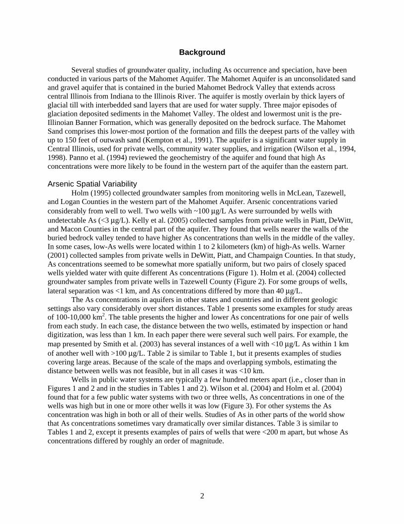
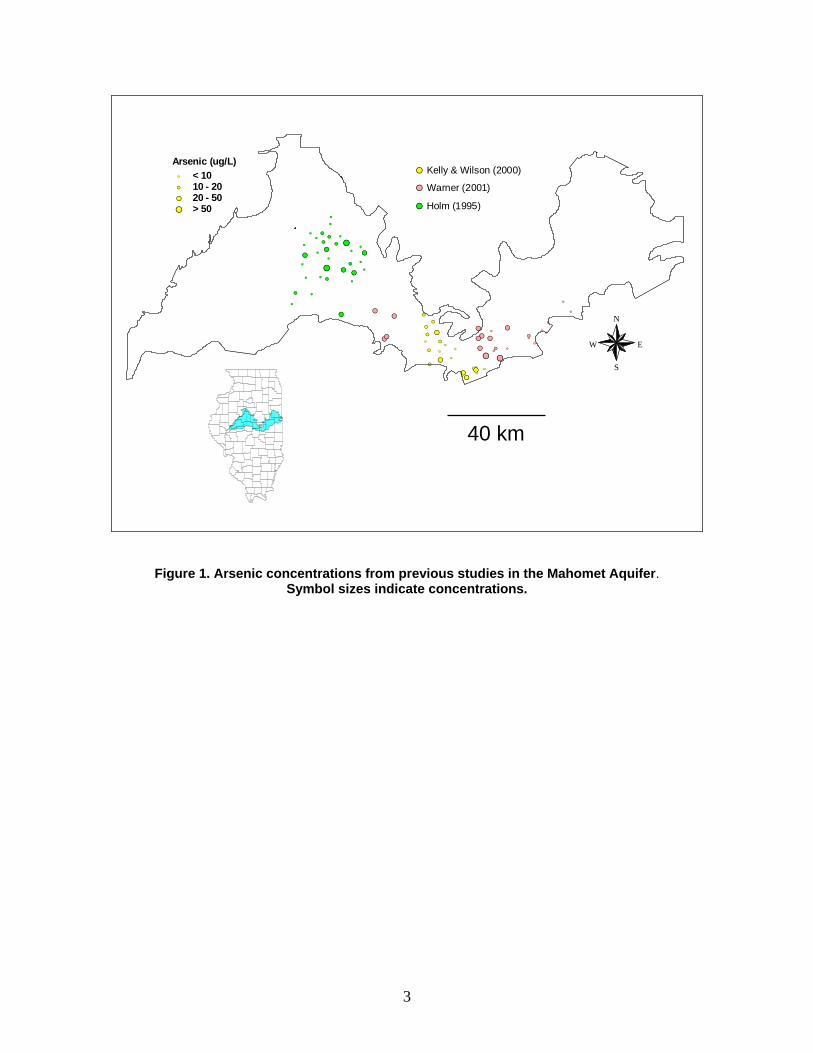
Holm (1995) collected groundwater samples from monitoring wells in McLean, Tazewell, and Logan Counties in the western part of the Mahomet Aquifer. Arsenic concentrations varied considerably from well to well. Two wells with ~100 μg/L As were surrounded by wells with undetectable As (<3 μg/L). Kelly et al. (2005) collected samples from private wells in Piatt, DeWitt, and Macon Counties in the central part of the aquifer. They found that wells nearer the walls of the buried bedrock valley tended to have higher As concentrations than wells in the middle of the valley. In some cases, low-As wells were located within 1 to 2 kilometers (km) of high-As wells. Warner (2001) collected samples from private wells in DeWitt, Piatt, and Champaign Counties. In that study, As concentrations seemed to be somewhat more spatially uniform, but two pairs of closely spaced wells yielded water with quite different As concentrations (Figure 1). Holm et al. (2004) collected groundwater samples from private wells in Tazewell County (Figure 2). For some groups of wells, lateral separation was <1 km, and As concentrations differed by more than 40 μg/L.
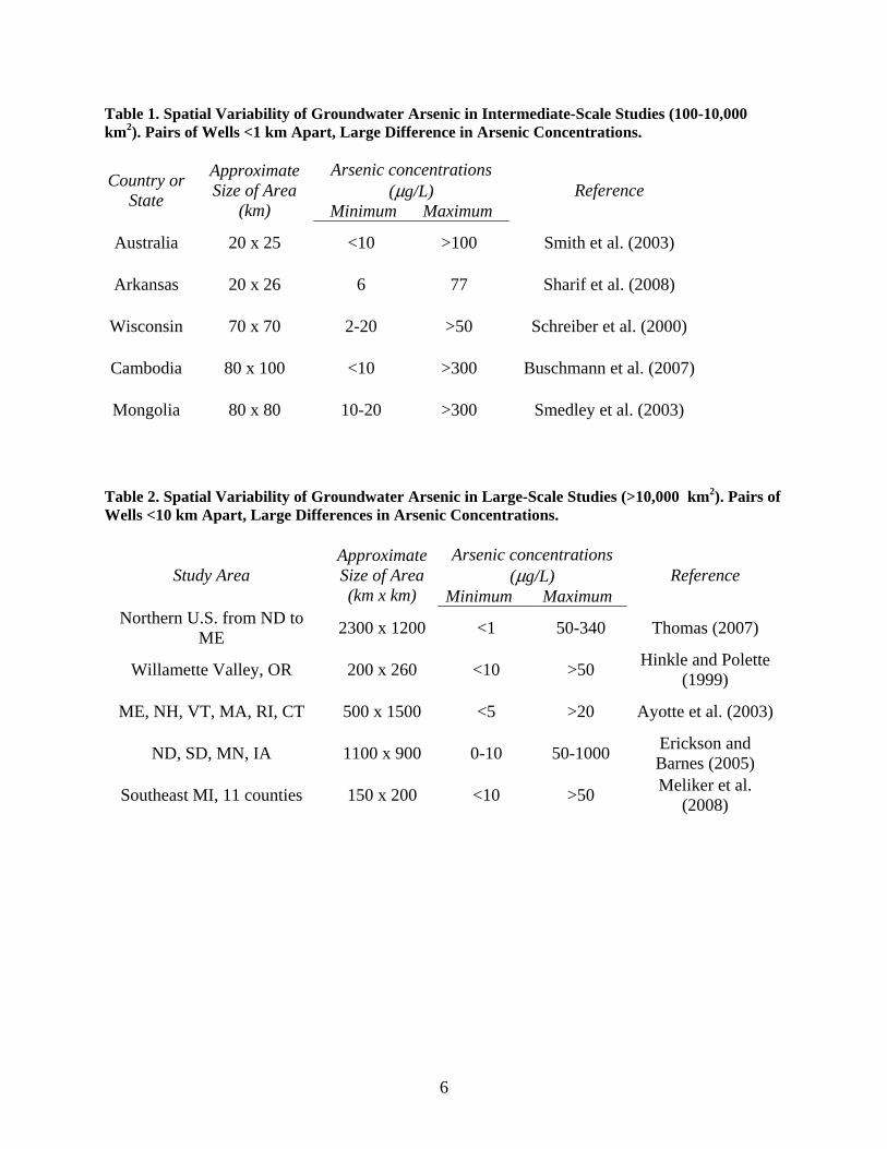
The As concentrations in aquifers in other states and countries and in different geologic settings also vary considerably over short distances. Table 1 presents some examples for study areas of 100-10,000 km2. The table presents the higher and lower As concentrations for one pair of wells from each study. In each case, the distance between the two wells, estimated by inspection or hand digitization, was less than 1 km. In each paper there were several such well pairs. For example, the map presented by Smith et al. (2003) has several instances of a well with <10 μg/L As within 1 km of another well with >100 μg/L. Table 2 is similar to Table 1, but it presents examples of studies covering large areas. Because of the scale of the maps and overlapping symbols, estimating the distance between wells was not feasible, but in all cases it was <10 km.
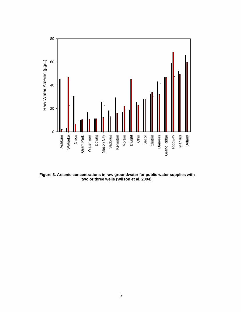
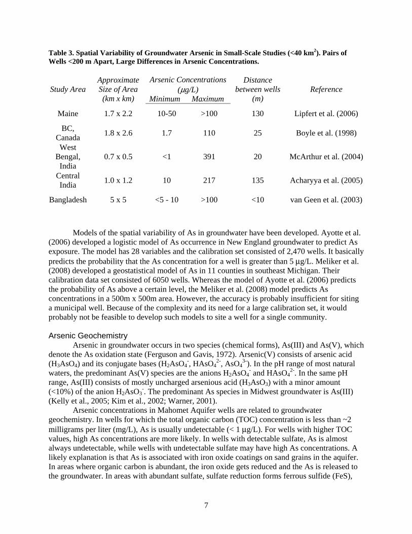
Wells in public water systems are typically a few hundred meters apart (i.e., closer than in Figures 1 and 2 and in the studies in Tables 1 and 2). Wilson et al. (2004) and Holm et al. (2004) found that for a few public water systems with two or three wells, As concentrations in one of the wells was high but in one or more other wells it was low (Figure 3). For other systems the As concentration was high in both or all of their wells. Studies of As in other parts of the world show that As concentrations sometimes vary dramatically over similar distances. Table 3 is similar to Tables 1 and 2, except it presents examples of pairs of wells that were <200 m apart, but whose As concentrations differed by roughly an order of magnitude.
3
#S #S
#S
#S
#S#S
#S
#S#S
#S
#S
#S#S
#S
#S
#S
#S#S
#S#S
#S
#S
#S
#S
#S#S
#S
#S
#S
#S
#S
#S
#S
#S
#S#S
#S#S
#S
#S
#S#S
#S
#S #S
#S
#S
#S
#S#S
#S
#S
#S
#S
#S
#S
#S
#S#S#S#S
#S
#S#S
#S
#S
#S
#S
#S
#S
#S
#S
#S
#S
#S #S#S
#S
N
EW
S
#S
#S
#S < 10#S 10 - 20#S 20 - 50#S > 50
#SArsenic (ug/L)
Kelly & Wilson (2000)
Warner (2001)
Holm (1995)
40 km
Figure 1. Arsenic concentrations from previous studies in the Mahomet Aquifer.
Symbol sizes indicate concentrations.
4
#S < 10#S 10 - 50#S > 50
Arsenic (μg/L)
10 km
Pekin
Tremont
Hopedale
N
EW
S
Figure 2. Arsenic concentrations in Tazewell County private wells (Holm et al. 2004).
5
Ash
kum
Wat
seka
Cis
co
Gra
nt P
ark
Wat
erm
an
Dow
ns
Mas
on C
ity
Sado
rus
Kem
pton
Mor
ton
Dw
ight
Ohi
o
Seco
r
Clin
ton
Dan
vers
Gra
nd R
idge
Rid
gway
Man
lius
Del
and
Raw
Wat
er A
rsen
ic (μ
g/L)
0
20
40
60
80
Figure 3. Arsenic concentrations in raw groundwater for public water supplies with two or three wells (Wilson et al. 2004).
6
Table 1. Spatial Variability of Groundwater Arsenic in Intermediate-Scale Studies (100-10,000 km2). Pairs of Wells <1 km Apart, Large Difference in Arsenic Concentrations.
Country or State
Approximate Size of Area
(km)
Arsenic concentrations (μg/L)
Minimum Maximum Reference
Australia 20 x 25 <10 >100 Smith et al. (2003)
Arkansas 20 x 26 6 77 Sharif et al. (2008)
Wisconsin 70 x 70 2-20 >50 Schreiber et al. (2000)
Cambodia 80 x 100 <10 >300 Buschmann et al. (2007)
Mongolia 80 x 80 10-20 >300 Smedley et al. (2003)
Table 2. Spatial Variability of Groundwater Arsenic in Large-Scale Studies (>10,000 km2). Pairs of Wells <10 km Apart, Large Differences in Arsenic Concentrations.
Study Area Approximate Size of Area (km x km)
Arsenic concentrations (μg/L) Reference
Minimum Maximum Northern U.S. from ND to
ME 2300 x 1200 <1 50-340 Thomas (2007)
Willamette Valley, OR 200 x 260 <10 >50 Hinkle and Polette
(1999)
ME, NH, VT, MA, RI, CT 500 x 1500 <5 >20 Ayotte et al. (2003)
ND, SD, MN, IA 1100 x 900 0-10 50-1000 Erickson and Barnes (2005)
Southeast MI, 11 counties 150 x 200 <10 >50 Meliker et al.
(2008)
7
Table 3. Spatial Variability of Groundwater Arsenic in Small-Scale Studies (<40 km2). Pairs of Wells <200 m Apart, Large Differences in Arsenic Concentrations.
Study Area Approximate Size of Area (km x km)
Arsenic Concentrations (μg/L)
Distance between wells
(m) Reference
Minimum Maximum
Maine 1.7 x 2.2 10-50 >100 130 Lipfert et al. (2006)
BC, Canada
1.8 x 2.6 1.7 110 25 Boyle et al. (1998)
West Bengal,
India 0.7 x 0.5 <1 391 20 McArthur et al. (2004)
Central India
1.0 x 1.2 10 217 135 Acharyya et al. (2005)
Bangladesh 5 x 5 <5 - 10 >100 <10 van Geen et al. (2003)
Models of the spatial variability of As in groundwater have been developed. Ayotte et al. (2006) developed a logistic model of As occurrence in New England groundwater to predict As exposure. The model has 28 variables and the calibration set consisted of 2,470 wells. It basically predicts the probability that the As concentration for a well is greater than 5 μg/L. Meliker et al. (2008) developed a geostatistical model of As in 11 counties in southeast Michigan. Their calibration data set consisted of 6050 wells. Whereas the model of Ayotte et al. (2006) predicts the probability of As above a certain level, the Meliker et al. (2008) model predicts As concentrations in a 500m x 500m area. However, the accuracy is probably insufficient for siting a municipal well. Because of the complexity and its need for a large calibration set, it would probably not be feasible to develop such models to site a well for a single community.
Arsenic Geochemistry
Arsenic in groundwater occurs in two species (chemical forms), As(III) and As(V), which denote the As oxidation state (Ferguson and Gavis, 1972). Arsenic(V) consists of arsenic acid (H3AsO4) and its conjugate bases (H2AsO4
-, HAsO42-, AsO4
3-). In the pH range of most natural waters, the predominant As(V) species are the anions H2AsO4
- and HAsO42-. In the same pH
range, As(III) consists of mostly uncharged arsenious acid (H3AsO3) with a minor amount (<10%) of the anion H2AsO3
-. The predominant As species in Midwest groundwater is As(III) (Kelly et al., 2005; Kim et al., 2002; Warner, 2001).
Arsenic concentrations in Mahomet Aquifer wells are related to groundwater geochemistry. In wells for which the total organic carbon (TOC) concentration is less than ~2 milligrams per liter (mg/L), As is usually undetectable (< 1 μg/L). For wells with higher TOC values, high As concentrations are more likely. In wells with detectable sulfate, As is almost always undetectable, while wells with undetectable sulfate may have high As concentrations. A likely explanation is that As is associated with iron oxide coatings on sand grains in the aquifer. In areas where organic carbon is abundant, the iron oxide gets reduced and the As is released to the groundwater. In areas with abundant sulfate, sulfate reduction forms ferrous sulfide (FeS),
8
which sorbs As(III) (Bostick and Fendorf, 2003; Holm et al., 2005; Kelly et al., 2005; Kirk et al., 2004).
Arsenic in groundwater may be truly dissolved or associated with particulate or colloidal matter and there are good reasons to characterize this aspect of As speciation. The unfiltered (total) As concentration indicates As exposure via drinking water, assuming particulate As is bioavailable. Particulate As would probably be easy to remove by commercially available household filter units. Filtered (dissolved) As concentrations would be a good estimate of As exposure in homes with filtered water. Also, dissolved As concentrations are needed to assess As solubility and in geochemical modeling.
Chen et al. (1999) found that in a nation-wide survey of As occurrence and speciation (Frey et al. 1998), particulate As, defined as the difference between filtered and unfiltered As concentrations, accounted for a significant fraction of As in many samples. In contrast, Holm et al. (2004) found no significant differences between filtered and unfiltered As concentrations in Mahomet Aquifer samples. However, in the Frey et al. (1998) study, the unfiltered samples were digested (heated with strong acid) to dissolve any particles. In the Holm et al. (2004) study, the samples were not digested, so particulate As may have been underestimated. An objective of the present work was to see if there was detectable particulate As in the groundwater and if sample digestion was necessary to quantify particulate As. These questions have practical consequences. Collecting and analyzing both filtered and unfiltered samples doubles analytical costs, compared to collecting only one or the other. Sample digestion also adds to analytical costs and is a potential source of contamination.
9
Methods and Materials
Well Selection The goal in selecting wells was to select areas with groups of wells that fit the following
criteria: 1) All houses in location have private wells, 2) Located in an area known to have high As in some wells, 3) Well logs on file at ISWS or the county health department, 4) Separate geographical areas, and if possible, 5) Different geological settings (e.g., sand and gravel vs. bedrock). Data from a number of sources were analyzed to determine possible areas for inclusion in the study.
Because of the extensive research completed in Tazewell County, that area was evaluated first. A review of well records indicated a number of subdivisions existed in areas where previous sampling showed elevated arsenic concentrations in private wells. The well locations in the ISWS private well database were mapped to identify subdivisions of interest, and then a site visit was conducted to determine the viability of each subdivision. Two subdivisions were selected in Tazewell County: one between Tremont and Pekin and one near Hopedale. (See Figure 2.) The aquifer under one subdivision selected was relatively thin and some bedrock wells were located in the same area as the Mahomet Aquifer wells. In the other subdivision, the aquifer was thicker and there were no bedrock wells. Wells in both subdivisions were of roughly the same depth and in the same aquifer, and well logs were available for each well.
For each area in Tazewell County, researchers went door-to-door seeking permission to sample homeowners’ wells. In return for access, the well owner received a water analysis for their private well. Once the wells were identified and permission secured, well owners were informed of the sampling dates and arrangements were made to sample well water.
A water quality survey of non-transient, non-community water supplies (e.g., schools, campgrounds) conducted by the McHenry County Health Department found that the well for an elementary school in the Wonder Lake area had a moderately elevated As concentration (15 μg/L). Follow-up sampling of other wells, including private homes and businesses, found As concentrations in excess of the MCL in two limited areas. Arsenic concentrations were below the MCL in all other wells sampled. Ten of the Wonder Lake wells were re-sampled for the present work to confirm earlier results and to characterize the As speciation and groundwater geochemistry of the area.
Sample Collection
Groundwater samples from most houses were collected from outside spigots. A garden hose and a flow-through cell with probes for measuring temperature, pH, conductivity, dissolved oxygen, and oxidation-reduction potential (ORP) were connected to the tap. The flow cell and data sonde were obtained from Hach/Hydrolab (Loveland, CO). The probes were calibrated at the Illinois State Water Survey laboratory before each sampling trip. Most of the flow went through the hose to waste. The water was set to flow for at least 15 minutes to flush out the well and pressure tank. After flushing, the readings were recorded and filtered (0.45 micrometers [μm]) and unfiltered samples were collected. For a few sites, samples were taken from a spigot upstream from the pressure tank. Water samples at these sites were collected as soon as the readings stabilized. Although we requested sampling points upstream from any treatment device, two of the Wonder Lake samples were found to be softened.
Table 4 presents the container materials and preservatives for the various water samples. Samples for As speciation were preserved with ethylenediaminetetraacetic acid (EDTA) (0.0013

10
moles per liter [M]) and acetic acid (0.083 M) and stored in the dark. Samanta and Clifford (2006) found that for groundwater samples preserved in this way, As speciation was stable for up to one month.
Table 4. Containers and Preservatives for Groundwater Samples. Analyte Filter? Container Preservative Arsenic species Yes High density
polyethylene (HDPE) Acetic acid (0.083 M) + 0.0013M Ethylenediaminetetraacetic acid
Total arsenic No HDPE 0.2% Nitric acid Metals Yes HDPE 0.2% Nitric acid Anions Yes HDPE None Alkalinity Yes HDPE None Organic carbon Yes Glass 0.2% Phosphoric acid Ammonia nitrogen Yes HDPE 0.2% Sulfuric acid
For both the Tremont and Hopedale sites, six replicate unfiltered samples were collected from 10 wells. Sample containers held sufficient ultra-pure nitric acid (HNO3) to give a concentration of 0.2% volume to volume dilution (v/v) upon sample addition. For each set of unfiltered Tremont samples, three samples were digested (5% HNO3 [v/v], 105°C for two hours) (Clesceri et al., 1998) in the sampling vessels (15 milliliter [mL] polypropylene culture tubes) and the other three were not digested. For each set of Hopedale samples, three samples were digested in the sampling vessels (50 mL polypropylene vials, same acid concentration and temperature as for Tremont), and the other three samples were poured into new vials before digestion. The objective was to test whether any colloidal or particulate As was retained in the collection vessels.
For each cluster of wells one set of sample bottles was filled with deionized water to check for contamination from containers and preservatives. Sample bottle sets were numbered consecutively. The odd-numbered sets had duplicate bottles for As species. Duplicate samples were used to check the overall precision of sampling, separation of As species, and analysis. Some duplicate samples were spiked immediately after collection with a mixture of As(III) and As(V) to check for any changes in speciation. For the Tremont and Hopedale well clusters, sets of six replicate unfiltered groundwater samples were collected from each well.
Chemical Analyses
Arsenic concentrations were determined by graphite furnace atomic absorption spectrophotometry (GFAAS) with palladium matrix modifier (Welz et al., 1988). Arsenic(III) levels were determined by anion exchange followed by GFAAS. The acetic acid preservative lowered the sample pH range to 3.0-3.5. In this pH range, As(V) is in the form of the H2AsO4
- and HAsO4
2- anions while essentially all of the As(III) is in the form of uncharged H3AsO3. Therefore, As(V) is retained by an anion exchange column while As(III) passes through (Ficklin, 1983). Arsenic(V) was determined as the difference between dissolved As and As(III). Unfiltered samples for total As determination were digested by adding ultra-pure HNO3 (5% v/v) and

11
heating at 105°C for two hours (Clesceri et al., 1998). After digestion, As concentrations were determined by GFAAS. The methods for all analytes besides As species are given in Table 5.
Table 5. Methods for Analytes Besides Arsenic. Alkalinity, mg/L as CaCO3, Electrometric Titration, Method USGS I-1030-85, Techniques of Water Resources, Investigation of the USGS, Chapter A-1, Methods for the Determination of Inorganic Substances in Water and Fluvial Sediments, Book 5, 3rd Edition, 1989. Determination of Metals and Trace Elements in Water and Wastes by Inductively Coupled Plasma-atomic Emission Spectrometry, U.S. EPA Method 200.7, Revision 4.4, Methods for the Determination of Metals in the Environmental Samples - Supplement I, EPA-600/R-94-111, May 1994. Determination of Inorganic Anions by Ion Chromatography, U.S. EPA Method 300.0, Revision 2.1, Methods for the Determination of Inorganic Substances in Environmental Samples, EPA-600/R-93-100, August 1993. Determination of Non-Volatile Organic Carbon, Combustion, SM 5310B, Standard Methods for the Examination of Water and Wastewater, 19th Edition. 1995. Available from the American Public Health Association, 1015 15th Street, N. W., Washington, D. C. 20005 Determination of Ammonia Nitrogen by Semi-Automated Colorimetry, US EPA Method 350.1, Revision 2.0, Methods for the Determination of Inorganic Substances in Environmental Samples, EPA-600/R-93-100, August 1993.

13
Results and Discussion
Spatial Variability of Arsenic For the Tremont well cluster (Figure 4), two central wells had 73 and 56 μg/L As, and As
concentrations within ~200 m were lower in all directions. However, a well ~500 m to the west had 82 μg/L As. If a municipal well was located between the 73 and 56 μg/L wells, a new well installed more than 150 m to the northwest or east or 200 m to the west would probably have a much lower As concentration. However, at greater distances to the west or southwest, the As concentrations might be higher.
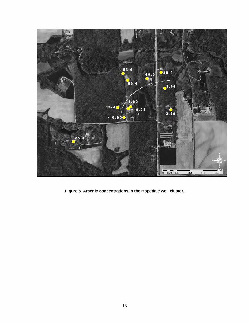
For the Hopedale well cluster (Figure 5), there is a distinct boundary between high-As and low-As wells. Some high- and low-As wells are separated by less than 100 m. In this area it appears that a new well installed south of this boundary would have low As, though additional sampling at a few of the houses further south of the current wells would be a worthwhile undertaking to confirm that the low As values are more regionally extensive.
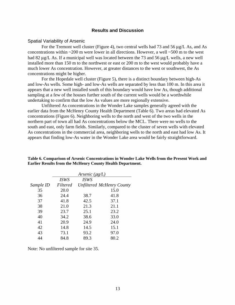
Unfiltered As concentrations in the Wonder Lake samples generally agreed with the earlier data from the McHenry County Health Department (Table 6). Two areas had elevated As concentrations (Figure 6). Neighboring wells to the north and west of the two wells in the northern part of town all had As concentrations below the MCL. There were no wells to the south and east, only farm fields. Similarly, compared to the cluster of seven wells with elevated As concentrations in the commercial area, neighboring wells to the north and east had low As. It appears that finding low-As water in the Wonder Lake area would be fairly straightforward. Table 6. Comparison of Arsenic Concentrations in Wonder Lake Wells from the Present Work and Earlier Results from the McHenry County Health Department.
Arsenic (μg/L)
Sample ID ISWS
Filtered ISWS
Unfiltered McHenry County35 20.0 15.0 36 24.4 38.7 41.8 37 41.8 42.5 37.1 38 21.0 21.3 21.1 39 23.7 25.1 23.2 40 34.2 38.6 33.0 41 20.9 24.9 24.0 42 14.8 14.5 15.1 43 73.1 93.2 97.0 44 84.8 89.3 80.2
Note: No unfiltered sample for site 35.

14
Figure 4. Arsenic concentrations in the Tremont well cluster. No samples were collected from the “TBS” well. The “BR” well is not screened in the Mahomet Aquifer.
15
Figure 5. Arsenic concentrations in the Hopedale well cluster.

16
Wonder Lake, IL
Figure 6. Arsenic concentrations in the Wonder Lake wells.
17
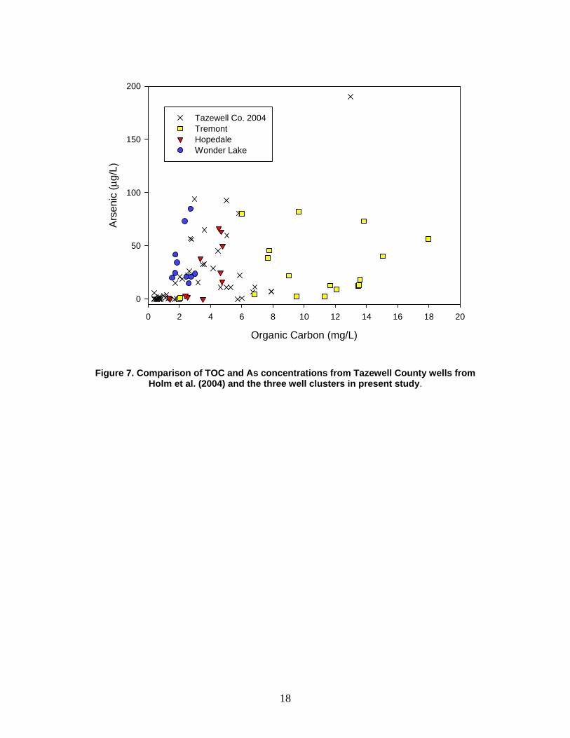
Arsenic Geochemistry Arsenic and Other Solutes For Tremont, Hopedale, and Wonder Lake wells and for TOC concentrations less than ~2 mg/L, As was near or below detection, whereas for higher TOC values, high As concentrations were common (Figure 7) in agreement with earlier Tazewell County results (Kelly et al., 2005) and other areas with high-As groundwater, such as south Asia (Ravenscroft et al., 2001). The Wonder Lake TOC values were all in the 2-3 mg/L range, which is near the minimum value for detectable As but still consistent with the other data. To the authors’ knowledge, this is the first report of this aspect of As geochemistry in northeast Illinois. The four Wonder Lake wells with the lowest TOC values were unique in other ways, as explained later in this report.
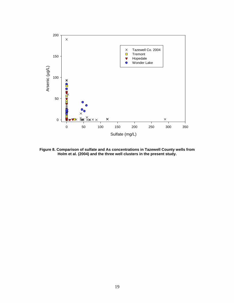
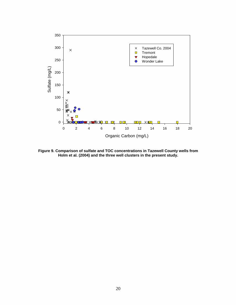
These As-TOC results are consistent with the iron oxide reduction/arsenic release hypothesis (McArthur et al., 2004). An adequate amount of natural organic matter (NOM) is needed to serve as the reductant. Oxidation of the organic matter produces CO2, which reacts with solid calcium carbonate to increase the alkalinity. Reduction of a small fraction of an iron oxide coating would probably release little As because the As would sorb to the remaining iron oxide. Arsenic would only accumulate in solution when a sufficient fraction of the iron oxide became reduced so that the remaining oxide was saturated with sorbed As. Therefore, the availability of solid organic matter may be an important factor in the observed patchy distribution of dissolved arsenic. Groundwater containing arsenic that was released in NOM-rich areas flowed to NOM-poor areas where the As re-sorbed to the iron oxide. Arsenic and sulfate were mutually exclusive in the Tremont and Hopedale wells and in six of the Wonder Lake wells (Figure 8), as noted in most of the earlier papers on Tazewell County (Kelly et al., 2005) and other areas (Dowling et al., 2002; McArthur et al., 2004). In contrast, in the four Wonder Lake wells with the lowest TOC values, sulfate and As were both easily detectable. Two of the earlier Tazewell County wells also had detectable As and sulfate (Holm et al., 2004; Kelly et al., 2005). For TOC concentrations greater than 3 mg/L, sulfate was undetectable in all wells (Figure 9), which is consistent with sulfate reduction in areas with abundant NOM. Conversely, all wells with <1 mg/L TOC had detectable sulfate. Four Wonder Lake wells, two Hopedale wells, one Tremont well, and two earlier Tazewell County wells with less than 2.5 mg/L TOC had detectable sulfate. There may have been incomplete or no sulfate reduction in the vicinity of these wells.
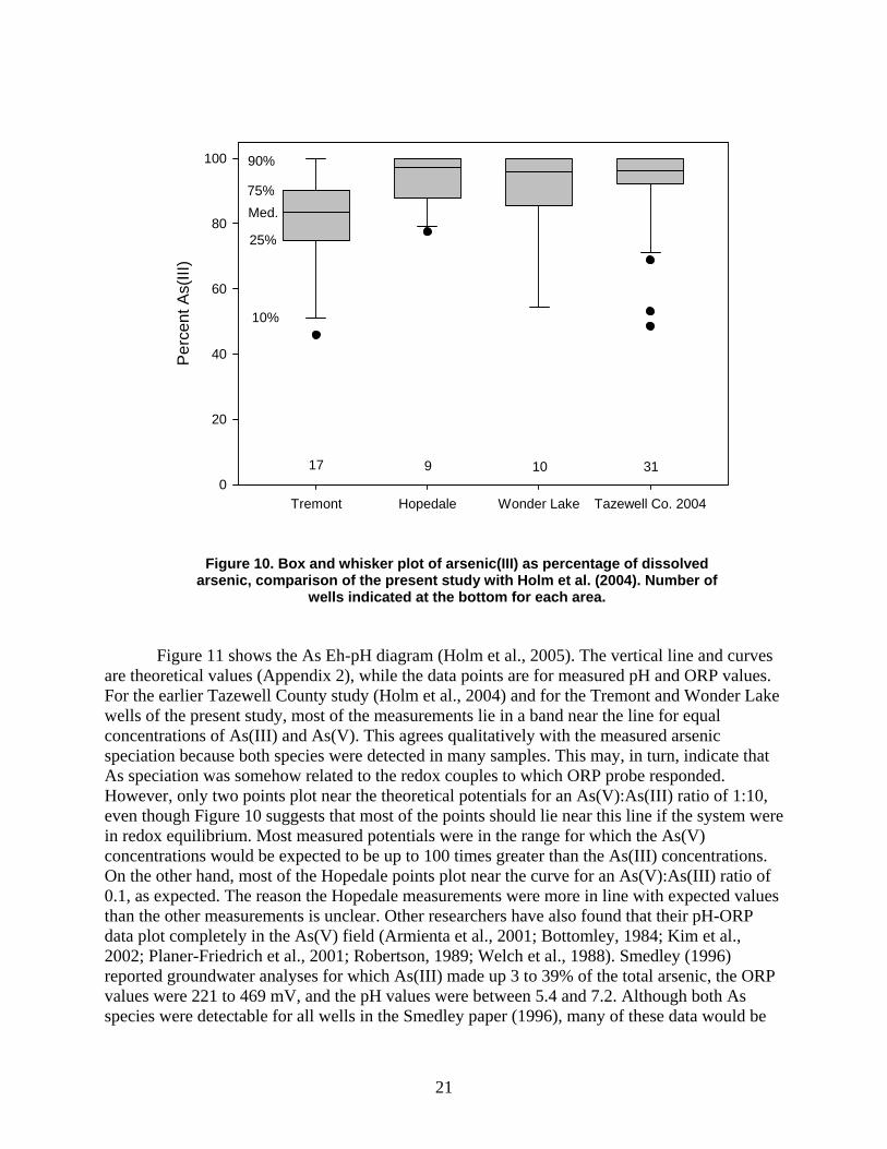
Although no sulfide analyses were performed, water from some wells had a faint but distinct hydrogen sulfide “rotten egg” odor. All groundwater samples had at least 0.1 mg/L Fe. Ferrous sulfide (FeS) is fairly insoluble (Stumm and Morgan, 1996), so any sulfide produced would mostly have precipitated as FeS. Arsenic(III) sorbs to FeS and iron pyrite (FeS2) (Bostick and Fendorf, 2003) and As sorption/coprecipitation accompanies bacterial sulfate reduction (Rittle et al., 1995). Therefore, sulfate reduction may affect As distribution in the Mahomet Aquifers and similar glacial aquifers. Dissolved As may have been released in areas where sulfate became depleted but re-sorbed in areas where there was active sulfate reduction. Arsenic Speciation and Redox Arsenic(III) was the predominant As species in all wells sampled (Figure 10), in agreement with earlier Tazewell County results (Holm et al., 2004). The median percent As(III) in the Tremont wells was less than the 25th percentile for the Hopedale wells. The Wonder Lake As speciation was similar to that of Hopedale. The two Wonder Lake outliers were for systems with softened water.
18
Organic Carbon (mg/L)
0 2 4 6 8 10 12 14 16 18 20
Ars
enic
(μg/
L)
0
50
100
150
200
Tazewell Co. 2004TremontHopedaleWonder Lake
Figure 7. Comparison of TOC and As concentrations from Tazewell County wells from Holm et al. (2004) and the three well clusters in present study.
19
Sulfate (mg/L)
0 50 100 150 200 250 300 350
Ars
enic
(μg/
L)
0
50
100
150
200
Tazewell Co. 2004TremontHopedaleWonder Lake
Figure 8. Comparison of sulfate and As concentrations in Tazewell County wells from Holm et al. (2004) and the three well clusters in the present study.
20
Organic Carbon (mg/L)
0 2 4 6 8 10 12 14 16 18 20
Sul
fate
(mg/
L)
0
50
100
150
200
250
300
350
Tazewell Co. 2004TremontHopedaleWonder Lake
Figure 9. Comparison of sulfate and TOC concentrations in Tazewell County wells from Holm et al. (2004) and the three well clusters in the present study.
21
Tremont Hopedale Wonder Lake Tazewell Co. 2004
Per
cent
As(
III)
0
20
40
60
80
100
10%
25%
Med.75%
90%
17 9 10 31
Figure 10. Box and whisker plot of arsenic(III) as percentage of dissolved arsenic, comparison of the present study with Holm et al. (2004). Number of
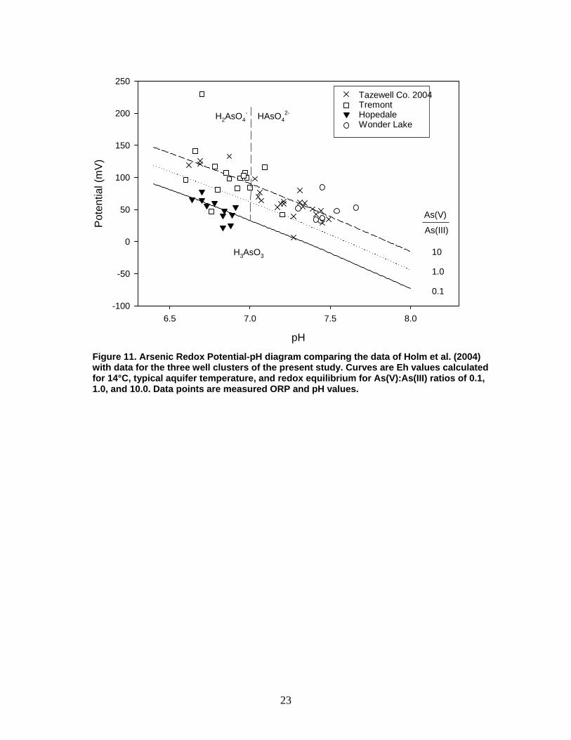
wells indicated at the bottom for each area. Figure 11 shows the As Eh-pH diagram (Holm et al., 2005). The vertical line and curves
are theoretical values (Appendix 2), while the data points are for measured pH and ORP values. For the earlier Tazewell County study (Holm et al., 2004) and for the Tremont and Wonder Lake wells of the present study, most of the measurements lie in a band near the line for equal concentrations of As(III) and As(V). This agrees qualitatively with the measured arsenic speciation because both species were detected in many samples. This may, in turn, indicate that As speciation was somehow related to the redox couples to which ORP probe responded. However, only two points plot near the theoretical potentials for an As(V):As(III) ratio of 1:10, even though Figure 10 suggests that most of the points should lie near this line if the system were in redox equilibrium. Most measured potentials were in the range for which the As(V) concentrations would be expected to be up to 100 times greater than the As(III) concentrations. On the other hand, most of the Hopedale points plot near the curve for an As(V):As(III) ratio of 0.1, as expected. The reason the Hopedale measurements were more in line with expected values than the other measurements is unclear. Other researchers have also found that their pH-ORP data plot completely in the As(V) field (Armienta et al., 2001; Bottomley, 1984; Kim et al., 2002; Planer-Friedrich et al., 2001; Robertson, 1989; Welch et al., 1988). Smedley (1996) reported groundwater analyses for which As(III) made up 3 to 39% of the total arsenic, the ORP values were 221 to 469 mV, and the pH values were between 5.4 and 7.2. Although both As species were detectable for all wells in the Smedley paper (1996), many of these data would be
22
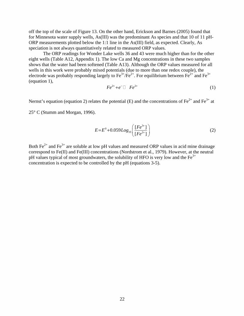
off the top of the scale of Figure 13. On the other hand, Erickson and Barnes (2005) found that for Minnesota water supply wells, As(III) was the predominant As species and that 10 of 11 pH-ORP measurements plotted below the 1:1 line in the As(III) field, as expected. Clearly, As speciation is not always quantitatively related to measured ORP values.
The ORP readings for Wonder Lake wells 36 and 43 were much higher than for the other eight wells (Table A12, Appendix 1). The low Ca and Mg concentrations in these two samples shows that the water had been softened (Table A13). Although the ORP values measured for all wells in this work were probably mixed potentials (due to more than one redox couple), the electrode was probably responding largely to Fe3+/Fe2+. For equilibrium between Fe2+ and Fe3+ (equation 1), 2 2Fe e Fe+ − ++ (1)
Nernst’s equation (equation 2) relates the potential (E) and the concentrations of Fe2+ and Fe3+ at
25° C (Stumm and Morgan, 1996).
3
010 2
[ ]0.059
[ ]
FeE E Log
Fe
+
+
= +
(2)
Both Fe2+ and Fe3+ are soluble at low pH values and measured ORP values in acid mine drainage correspond to Fe(II) and Fe(III) concentrations (Nordstrom et al., 1979). However, at the neutral pH values typical of most groundwaters, the solubility of HFO is very low and the Fe3+ concentration is expected to be controlled by the pH (equations 3-5).
23
pH
6.5 7.0 7.5 8.0
Pot
entia
l (m
V)
-100
-50
0
50
100
150
200
250
10
1.0
0.1
As(V)
Tazewell Co. 2004TremontHopedaleWonder Lake
As(III)
H2AsO4- HAsO4
2-
H3AsO3
Figure 11. Arsenic Redox Potential-pH diagram comparing the data of Holm et al. (2004) with data for the three well clusters of the present study. Curves are Eh values calculated for 14°C, typical aquifer temperature, and redox equilibrium for As(V):As(III) ratios of 0.1, 1.0, and 10.0. Data points are measured ORP and pH values.
24
3
3 2( ) 3 3Fe OH H Fe H O+ ++ + (3)
3
0 3
[ ]
[ ]s
FeK
H
+
+′= (4)
310 10 0[ ] 3sLog Fe Log K pH+ ′= − (5)
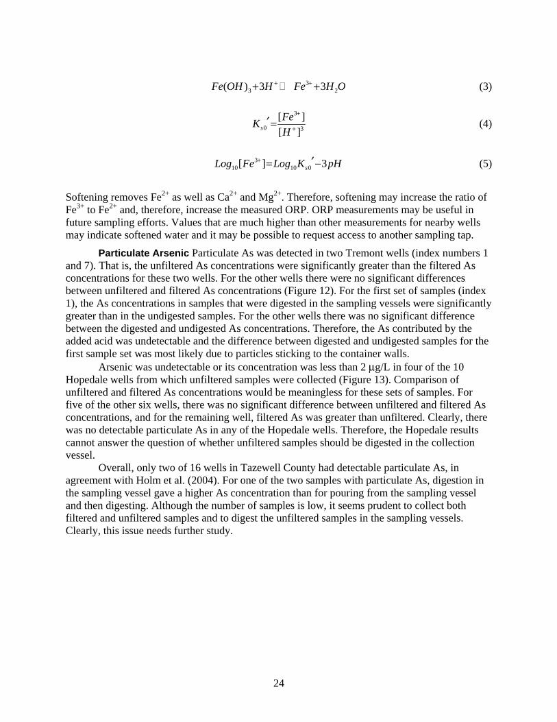
Softening removes Fe2+ as well as Ca2+ and Mg2+. Therefore, softening may increase the ratio of Fe3+ to Fe2+ and, therefore, increase the measured ORP. ORP measurements may be useful in future sampling efforts. Values that are much higher than other measurements for nearby wells may indicate softened water and it may be possible to request access to another sampling tap.
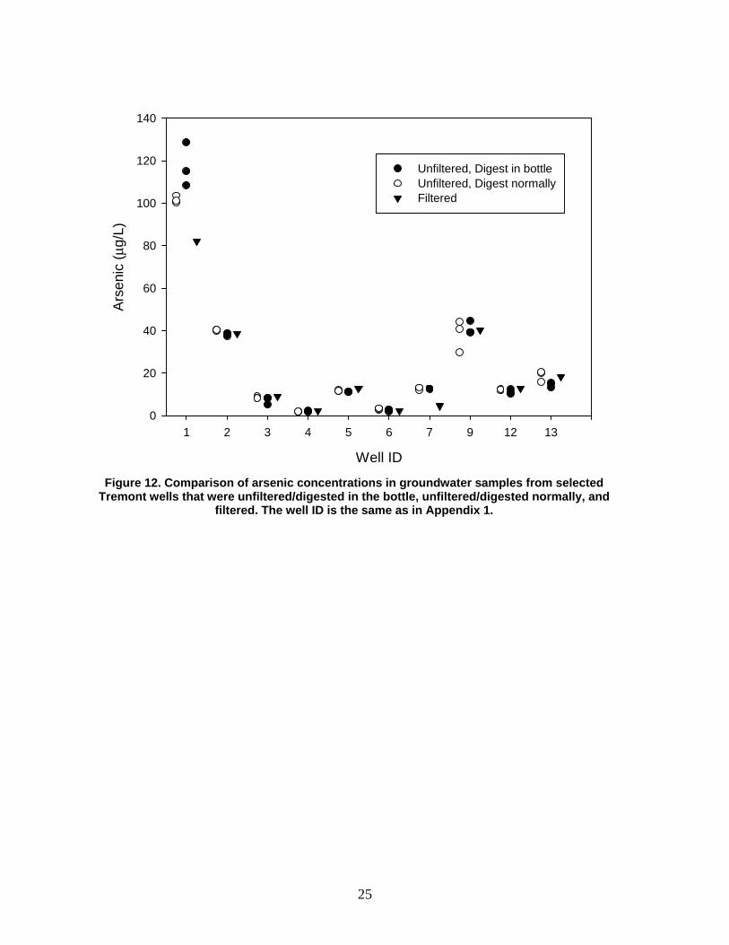
Particulate Arsenic Particulate As was detected in two Tremont wells (index numbers 1 and 7). That is, the unfiltered As concentrations were significantly greater than the filtered As concentrations for these two wells. For the other wells there were no significant differences between unfiltered and filtered As concentrations (Figure 12). For the first set of samples (index 1), the As concentrations in samples that were digested in the sampling vessels were significantly greater than in the undigested samples. For the other wells there was no significant difference between the digested and undigested As concentrations. Therefore, the As contributed by the added acid was undetectable and the difference between digested and undigested samples for the first sample set was most likely due to particles sticking to the container walls.
Arsenic was undetectable or its concentration was less than 2 μg/L in four of the 10 Hopedale wells from which unfiltered samples were collected (Figure 13). Comparison of unfiltered and filtered As concentrations would be meaningless for these sets of samples. For five of the other six wells, there was no significant difference between unfiltered and filtered As concentrations, and for the remaining well, filtered As was greater than unfiltered. Clearly, there was no detectable particulate As in any of the Hopedale wells. Therefore, the Hopedale results cannot answer the question of whether unfiltered samples should be digested in the collection vessel.
Overall, only two of 16 wells in Tazewell County had detectable particulate As, in agreement with Holm et al. (2004). For one of the two samples with particulate As, digestion in the sampling vessel gave a higher As concentration than for pouring from the sampling vessel and then digesting. Although the number of samples is low, it seems prudent to collect both filtered and unfiltered samples and to digest the unfiltered samples in the sampling vessels. Clearly, this issue needs further study.
25
Well ID
1 2 3 4 5 6 7 9 12 13
Ars
enic
(μg/
L)
0
20
40
60
80
100
120
140
Unfiltered, Digest in bottleUnfiltered, Digest normallyFiltered
Figure 12. Comparison of arsenic concentrations in groundwater samples from selected
Tremont wells that were unfiltered/digested in the bottle, unfiltered/digested normally, and filtered. The well ID is the same as in Appendix 1.

26
Well ID
21 22 24 25 30 32 33
Ars
enic
(μg/
L)
0
20
40
60
80
Unfiltered, Digest in bottleUnfiltered, Digest normallyFiltered
Figure 13. Comparison of arsenic concentrations in groundwater samples from selected Hopedale wells that were unfiltered/digested in the bottle, unfiltered/digested normally, and filtered. The well
ID is the same as in Appendix 1.
27
Conclusions Arsenic in Illinois groundwater can be highly variable over distances as short as tens of meters. The arsenic concentration at any point in these areas would be difficult to impossible to predict from a regional model, based on these results. Siting a new well would likely require that every nearby well of interest be sampled. Conversely, sampling existing private wells, when those wells exist, may be an economical way for a community to assess the possibility of siting a new well near their municipal well. For all three study areas, TOC values were 2 mg/L or greater and most As concentrations were above the MCL. This is in agreement with earlier work in Tazewell County and is consistent with the hypothesis that HFO reduction is the source of As in these aquifers. For all three study areas, sulfate was generally undetectable for TOC values greater than 2 mg/L and detectable in most samples with lower TOC values. For all Hopedale and Tremont wells and six Wonder Lake wells, either As or sulfate was detectable, but not both. These data are consistent with complete sulfate reduction in areas with abundant organic matter and incomplete sulfate reduction in other areas. The data are also consistent with limitation of dissolved As by sorption to FeS in areas with active sulfate reduction. As(III) was the main As species in all three study areas, in agreement with earlier results for Tazewell County. Values of pH and ORP were qualitatively consistent with As speciation for the Hopedale wells as indicated by an As Eh-pH diagram. For the other two areas, the ORP measurements were consistent with much lower proportions of As(III) (i.e., they were higher than expected). Fifteen out of 17 wells showed no significant differences between filtered and unfiltered As concentrations. Clearly, particulate As concentrations were generally too low to be calculated by difference. ORP measurements for the two softened Wonder Lake wells were much higher than for the eight untreated wells, as would be expected if the redox electrode responded largely to dissolved Fe. (Softening reduces the Fe2+ concentration.) ORP measurements combined with general knowledge of the system may be useful in future field studies to indicate treated water when untreated water is expected.

29
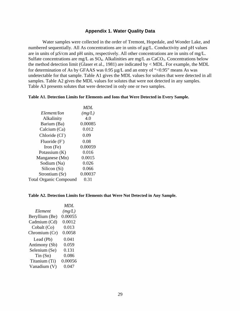
Appendix 1. Water Quality Data Water samples were collected in the order of Tremont, Hopedale, and Wonder Lake, and numbered sequentially. All As concentrations are in units of μg/L. Conductivity and pH values are in units of μS/cm and pH units, respectively. All other concentrations are in units of mg/L. Sulfate concentrations are mg/L as SO4. Alkalinities are mg/L as CaCO3. Concentrations below the method detection limit (Glaser et al., 1981) are indicated by < MDL. For example, the MDL for determination of As by GFAAS was 0.95 μg/L and an entry of “<0.95” means As was undetectable for that sample. Table A1 gives the MDL values for solutes that were detected in all samples. Table A2 gives the MDL values for solutes that were not detected in any samples. Table A3 presents solutes that were detected in only one or two samples. Table A1. Detection Limits for Elements and Ions that Were Detected in Every Sample.
Element/Ion MDL
(mg/L) Alkalinity 4.0
Barium (Ba) 0.00085 Calcium (Ca) 0.012 Chloride (Cl-) 0.09 Fluoride (F-) 0.08
Iron (Fe) 0.00059 Potassium (K) 0.016
Manganese (Mn) 0.0015 Sodium (Na) 0.026 Silicon (Si) 0.066
Strontium (Sr) 0.00037 Total Organic Compound 0.31 Table A2. Detection Limits for Elements that Were Not Detected in Any Sample.
Element MDL
(mg/L) Beryllium (Be) 0.00055 Cadmium (Cd) 0.0012
Cobalt (Co) 0.013 Chromium (Cr) 0.0058
Lead (Pb) 0.041 Antimony (Sb) 0.059 Selenium (Se) 0.131
Tin (Sn) 0.086 Titanium (Ti) 0.00056 Vanadium (V) 0.047

30
Table A3. Elements and Ions that Were Detected in Only One or Two Samples.
Element/Ion Sample ID Concentration
(mg/L) MDL (mg/L) Comment Li 8 0.087 0.018 Bedrock well
Mo 18 0.026 0.022 Mo 40 0.055 0.022 Tl 2 0.018 0.017
NO3-N 17 2.87 0.07 Also had high SO42-
Table A4. Arsenic Species Concentrations and Field Measurements for Tremont Samples.
As (μg/L) Field Measurements
ID Filtered Anion
Exchange UnfilteredTemperature
(°C) Conductivity
(μS/cm) pH ORP (mV) 1 82.0 73.6 115.1 12.2 1090 7.20 42 2 38.7 35.1 38.6 11.9 1006 6.78 117 3 9.1 7.4 8.1 11.2 819 6.94 99 4 2.4 1.1 2.0 11.7 778 6.85 107 5 12.7 10.4 11.1 11.6 815 6.97 107 6 2.3 1.5 2.7 9.5 763 6.98 100 7 4.6 2.4 12.7 11.7 1053 6.70 230 8 <0.95 <0.95 9 40.3 35.4 39.3 10.9 995 6.92 83
10 56.4 47.0 11 12.2 9.1 11.4 1122 6.80 81 12 12.8 10.1 10.8 11.5 951 6.96 103 13 18.3 13.7 15.0 12.2 935 7.09 116 14 80.2 68.5 12.4 969 6.87 98 15 21.9 22.0 9.6 1001 6.76 47 16 45.7 42.3 12.5 1024 6.60 96 17 1.3 2.5 10.2 943 6.66 141 18 73.2 63.0 12.1 863 7.00 84 19 28.3
Notes: No field measurements for wells 8 (well ran dry), 10, or 19 (battery died). No unfiltered samples for wells 8, 10, 11, 14-19. Filtered sample for well 19 not analyzed due to a lab accident.

31
Table A5. Concentrations of Major Metals and Ammonium in Tremont Samples.
Sample Concentration (mg/L) ID Fe Mn Ca Mg Na K NH4-N 1 4.78 0.038 57.1 28.4 159 2.28 6.26 2 3.89 0.048 113.0 54.1 33.0 2.34 7.17 3 2.45 0.024 68.3 35.5 73.2 1.69 1.42 4 1.55 0.033 65.1 33.0 70.7 1.66 1.47 5 1.72 0.021 68.8 35.3 76.3 1.74 1.53 6 2.30 0.028 62.5 29.8 69.1 1.61 1.41 7 0.27 0.276 120.0 53.9 45.0 2.31 2.53 8 0.07 0.009 20.0 10.9 860 6.51 1.26 9 4.59 0.034 90.9 49.4 74.6 2.29 4.73
10 10.62 0.117 109.0 57.7 58.5 2.84 9.61 11 2.69 0.052 83.1 43.5 77.6 2.09 2.68 12 2.52 0.054 81.2 42.5 75.9 1.91 2.28 13 1.74 0.149 81.0 43.6 78.8 2.10 2.71 14 3.68 0.077 107.0 56.3 29.6 1.84 4.69 15 7.90 0.071 98.1 43.3 66.0 2.08 7.17 16 5.12 0.090 111.0 53.8 28.4 2.29 6.42 17 2.16 0.341 108.0 47.7 14.0 1.04 0.90 18 2.81 0.015 69.6 39.9 77.2 1.94 2.51 19 3.57 0.044 86.3 46.0 74.4 1.92 2.66

32
Table A6. Concentrations of Minor Metals and Boron in Tremont Samples.
Sample Concentration (mg/L) ID Al B Ba Cu Ni Sr Zn 1 0.014 0.31 0.54 <0.00079 <0.014 0.535 0.0976 2 0.027 0.38 0.35 <0.00079 0.019 0.607 0.0188 3 0.017 0.57 0.14 <0.00079 0.024 0.212 <0.0073 4 0.016 0.53 0.15 <0.00079 0.021 0.208 <0.0073 5 0.019 0.56 0.14 <0.00079 0.019 0.230 <0.0073 6 0.016 0.51 0.14 <0.00079 0.023 0.199 0.0099 7 0.041 0.40 0.15 0.00620 0.024 0.466 0.0117 8 0.016 1.76 6.03 0.00135 <0.014 0.670 0.0157 9 0.022 0.82 0.23 <0.00079 0.018 0.486 <0.0073
10 0.028 1.13 0.18 <0.00079 0.031 0.876 0.0080 11 0.021 0.71 0.23 <0.00079 0.021 0.303 0.0103 12 0.019 0.64 0.20 <0.00079 0.017 0.303 <0.0073 13 0.022 0.70 0.21 <0.00079 0.030 0.304 <0.0073 14 0.026 0.29 0.32 <0.00079 0.026 0.578 <0.0073 15 0.024 0.25 0.68 <0.00079 0.023 0.503 0.0957 16 0.027 0.31 0.28 <0.00079 0.029 0.635 <0.0073 17 0.027 0.12 0.07 <0.00079 0.020 0.216 0.0436 18 0.018 0.69 0.15 <0.00079 0.016 0.266 0.0981 19 0.022 0.69 0.17 <0.00079 0.023 0.315 0.0082
33
Table A7. Concentrations of Anions, Silica, and Organic Carbon in Tremont Samples. Concentration (mg/L)
ID Cl- F- SO42- P Alkalinity Si TOC
1 31.5 0.55 <0.31 1.66 572 6.51 9.65 2 2.71 0.40 <0.31 0.55 574 10.8 7.67 3 4.56 0.37 <0.31 0.27 466 8.80 12.1 4 3.83 0.39 <0.31 0.28 442 8.92 11.3 5 4.35 0.35 <0.31 0.20 462 9.45 11.7 6 3.38 0.42 <0.31 0.23 436 8.55 9.51 7 0.13 560 9.84 6.81 8 874 1.00 <0.31 0.08 732 5.05 1.97 9 4.33 0.38 <0.31 0.43 575 9.24 15.1
10 3.35 0.52 <0.31 0.77 632 10.1 18.0 11 4.79 0.37 <0.31 0.23 537 9.45 13.5 12 4.24 0.37 <0.31 0.25 524 9.39 13.5 13 4.86 0.37 0.42 0.22 534 9.34 13.6 14 2.63 0.42 0.51 0.31 564 10.1 6.01 15 5.58 0.31 <0.31 1.47 562 11.6 9.02 16 3.00 0.44 <0.31 0.53 573 10.5 7.77 17 23.9 0.36 23.4 <0.063 435 12.0 2.06 18 3.87 0.41 <0.31 0.16 493 9.18 13.8 19 4.15 0.38 <0.31 0.25 543 9.10 14.3
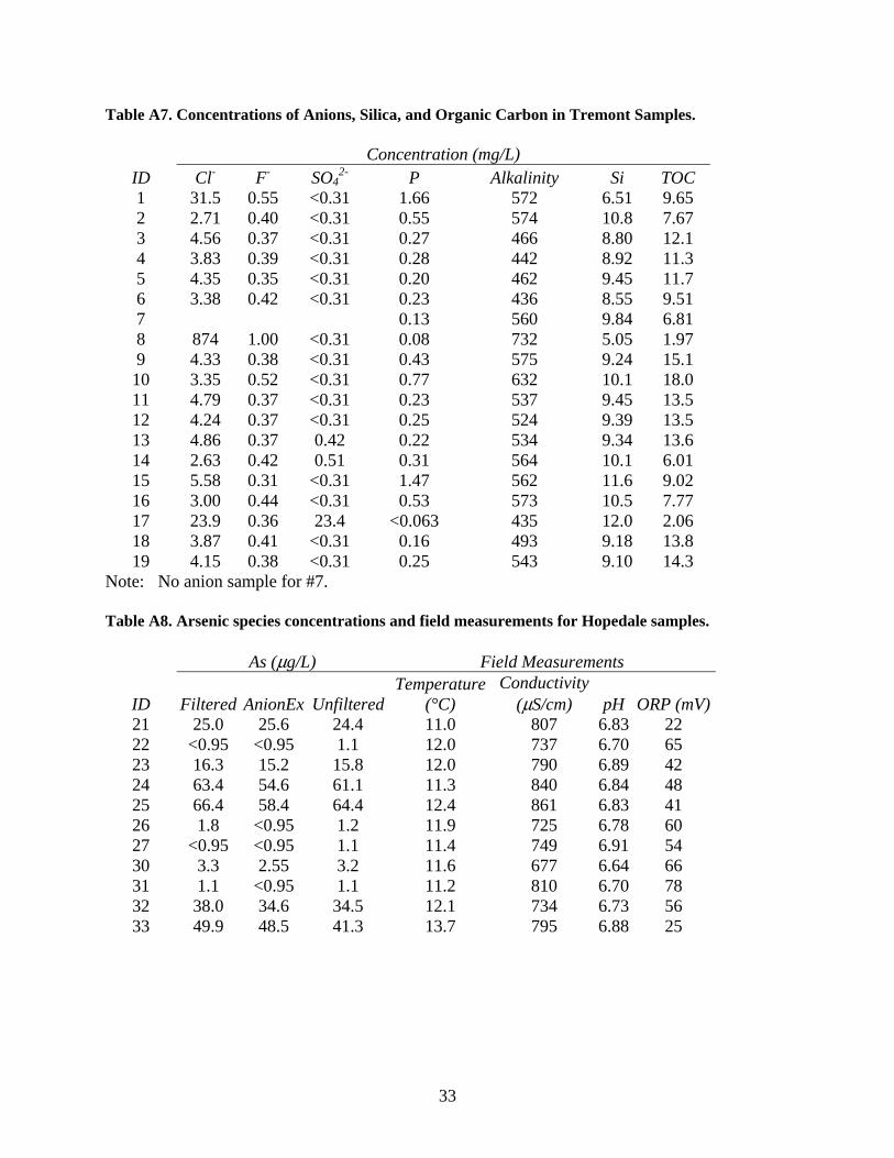
Note: No anion sample for #7. Table A8. Arsenic species concentrations and field measurements for Hopedale samples.
As (μg/L) Field Measurements
ID Filtered AnionEx UnfilteredTemperature
(°C) Conductivity
(μS/cm) pH ORP (mV) 21 25.0 25.6 24.4 11.0 807 6.83 22 22 <0.95 <0.95 1.1 12.0 737 6.70 65 23 16.3 15.2 15.8 12.0 790 6.89 42 24 63.4 54.6 61.1 11.3 840 6.84 48 25 66.4 58.4 64.4 12.4 861 6.83 41 26 1.8 <0.95 1.2 11.9 725 6.78 60 27 <0.95 <0.95 1.1 11.4 749 6.91 54 30 3.3 2.55 3.2 11.6 677 6.64 66 31 1.1 <0.95 1.1 11.2 810 6.70 78 32 38.0 34.6 34.5 12.1 734 6.73 56 33 49.9 48.5 41.3 13.7 795 6.88 25
34
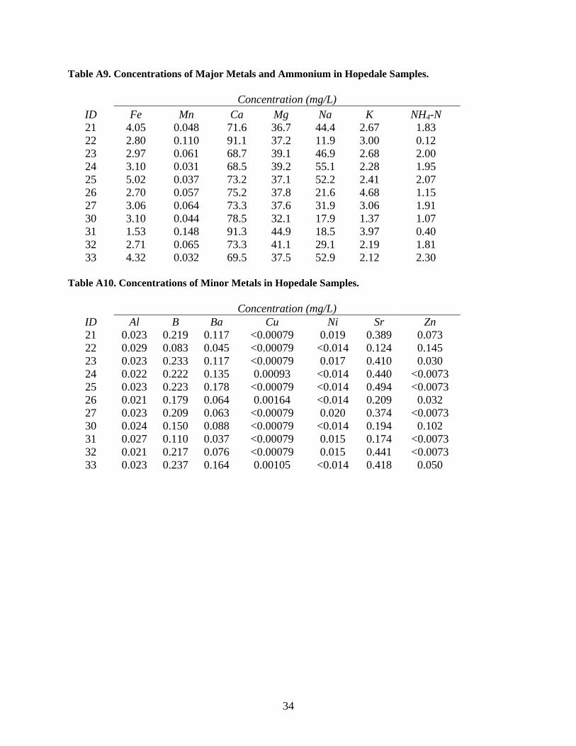
Table A9. Concentrations of Major Metals and Ammonium in Hopedale Samples.
Concentration (mg/L) ID Fe Mn Ca Mg Na K NH4-N 21 4.05 0.048 71.6 36.7 44.4 2.67 1.83 22 2.80 0.110 91.1 37.2 11.9 3.00 0.12 23 2.97 0.061 68.7 39.1 46.9 2.68 2.00 24 3.10 0.031 68.5 39.2 55.1 2.28 1.95 25 5.02 0.037 73.2 37.1 52.2 2.41 2.07 26 2.70 0.057 75.2 37.8 21.6 4.68 1.15 27 3.06 0.064 73.3 37.6 31.9 3.06 1.91 30 3.10 0.044 78.5 32.1 17.9 1.37 1.07 31 1.53 0.148 91.3 44.9 18.5 3.97 0.40 32 2.71 0.065 73.3 41.1 29.1 2.19 1.81 33 4.32 0.032 69.5 37.5 52.9 2.12 2.30
Table A10. Concentrations of Minor Metals in Hopedale Samples. Concentration (mg/L)
ID Al B Ba Cu Ni Sr Zn 21 0.023 0.219 0.117 <0.00079 0.019 0.389 0.073 22 0.029 0.083 0.045 <0.00079 <0.014 0.124 0.145 23 0.023 0.233 0.117 <0.00079 0.017 0.410 0.030 24 0.022 0.222 0.135 0.00093 <0.014 0.440 <0.0073 25 0.023 0.223 0.178 <0.00079 <0.014 0.494 <0.0073 26 0.021 0.179 0.064 0.00164 <0.014 0.209 0.032 27 0.023 0.209 0.063 <0.00079 0.020 0.374 <0.0073 30 0.024 0.150 0.088 <0.00079 <0.014 0.194 0.102 31 0.027 0.110 0.037 <0.00079 0.015 0.174 <0.0073 32 0.021 0.217 0.076 <0.00079 0.015 0.441 <0.0073 33 0.023 0.237 0.164 0.00105 <0.014 0.418 0.050

35
Table A11. Concentrations of Anions, Silica, and Organic Carbon in Hopedale Samples. Concentration (mg/L)
ID Cl- F- SO42- Alkalinity P Si TOC
21 27.6 0.31 <0.31 411 0.291 7.08 4.64 22 28.6 0.15 9.36 358 <0.063 7.09 1.39 23 26.8 0.34 <0.31 402 0.189 7.10 4.75 24 39.1 0.31 <0.31 411 0.224 7.09 4.69 25 45.0 0.29 <0.31 410 0.254 7.50 4.53 26 17.2 0.29 <0.31 382 0.068 6.94 2.54 27 17.6 0.35 <0.31 395 0.098 7.28 3.50 30 7.85 0.23 <0.31 368 0.111 7.75 2.39 31 32.8 0.20 18.0 389 <0.063 6.26 1.33 32 14.4 0.33 <0.31 392 0.140 7.47 3.35 33 29.9 0.33 <0.31 404 0.207 7.58 4.76
Table A12. Arsenic Species Concentrations and Field Measurements for Wonder Lake Samples.
As (μg/L) Field Measurements
ID Filtered AnionEx UnfilteredTemperature
(°C) Conductivity
(μS/cm) pH ORP (mV) 35 20.0 17.0 11.3 557 7.45 85 36 24.4 44.8 38.7 13.3 1085 7.54 322 37 41.8 35.8 42.5 11.6 997 7.30 52 38 21.0 19.6 21.3 12.8 595 7.44 33 39 23.7 23.1 25.1 14.5 602 7.45 36 40 34.2 32.9 38.6 14.0 980 7.45 37 41 20.9 25.0 24.9 17.4 917 7.41 34 42 14.8 15.2 14.5 13.0 471 7.66 53 43 73.1 39.7 93.2 12.1 492 7.98 236 44 84.8 88.7 11.7 487 7.54 48
Note: No unfiltered samples for 35 and 44.
36
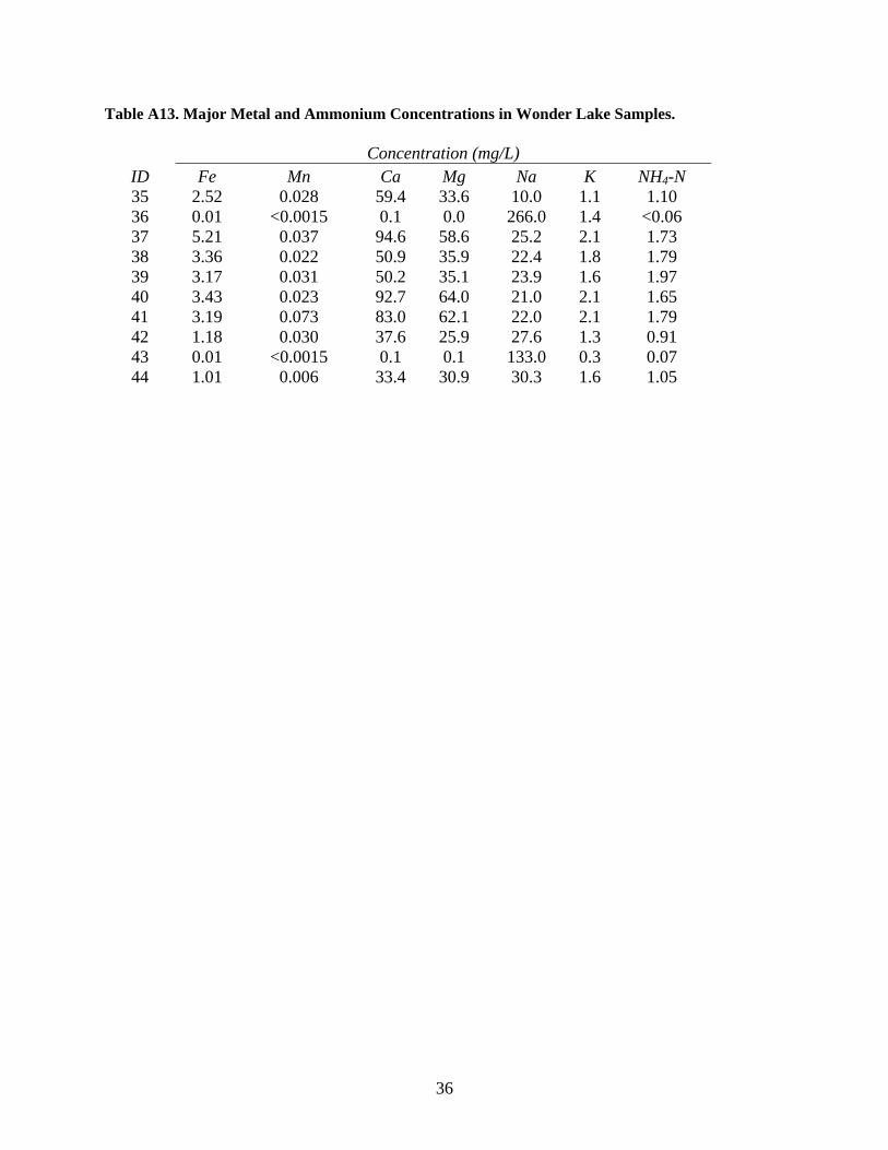
Table A13. Major Metal and Ammonium Concentrations in Wonder Lake Samples.
Concentration (mg/L) ID Fe Mn Ca Mg Na K NH4-N 35 2.52 0.028 59.4 33.6 10.0 1.1 1.10 36 0.01 <0.0015 0.1 0.0 266.0 1.4 <0.06 37 5.21 0.037 94.6 58.6 25.2 2.1 1.73 38 3.36 0.022 50.9 35.9 22.4 1.8 1.79 39 3.17 0.031 50.2 35.1 23.9 1.6 1.97 40 3.43 0.023 92.7 64.0 21.0 2.1 1.65 41 3.19 0.073 83.0 62.1 22.0 2.1 1.79 42 1.18 0.030 37.6 25.9 27.6 1.3 0.91 43 0.01 <0.0015 0.1 0.1 133.0 0.3 0.07 44 1.01 0.006 33.4 30.9 30.3 1.6 1.05
37
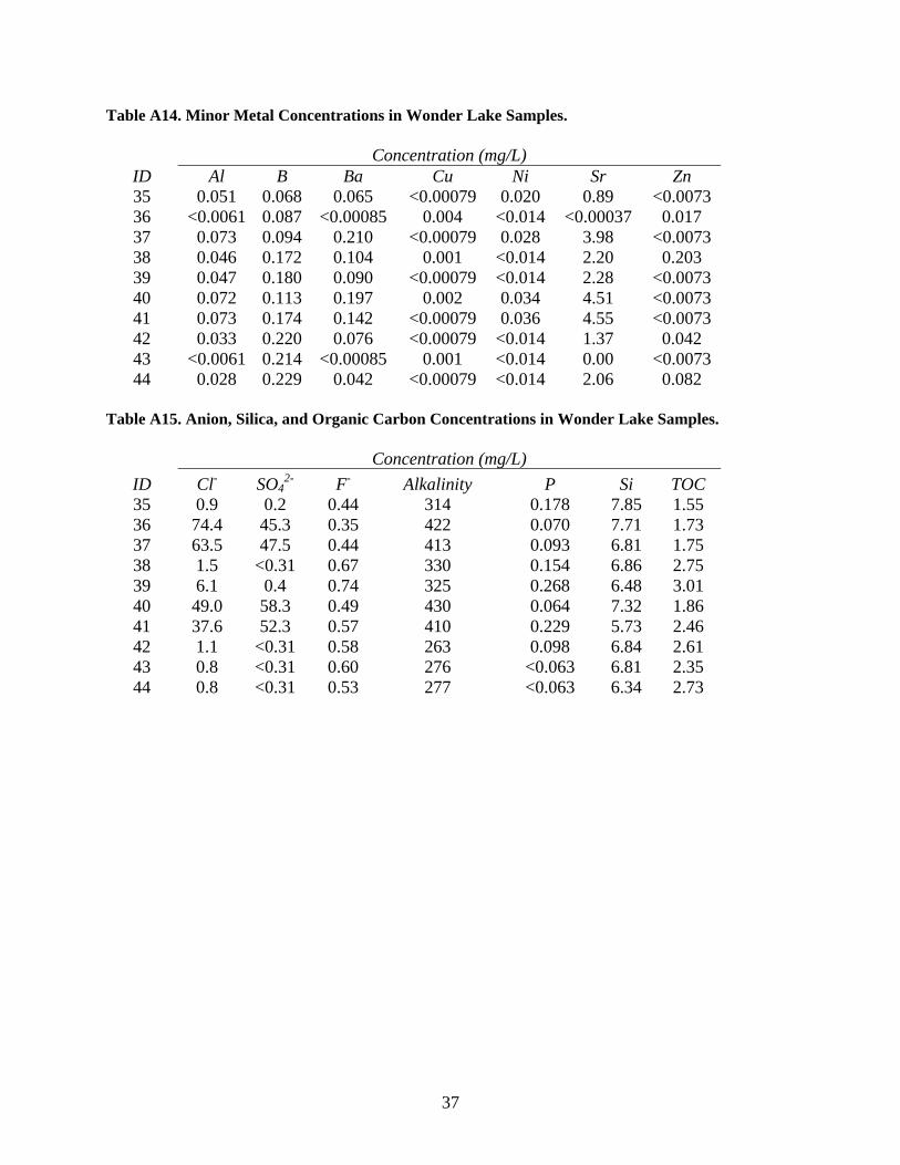
Table A14. Minor Metal Concentrations in Wonder Lake Samples. Concentration (mg/L)
ID Al B Ba Cu Ni Sr Zn 35 0.051 0.068 0.065 <0.00079 0.020 0.89 <0.0073 36 <0.0061 0.087 <0.00085 0.004 <0.014 <0.00037 0.017 37 0.073 0.094 0.210 <0.00079 0.028 3.98 <0.0073 38 0.046 0.172 0.104 0.001 <0.014 2.20 0.203 39 0.047 0.180 0.090 <0.00079 <0.014 2.28 <0.0073 40 0.072 0.113 0.197 0.002 0.034 4.51 <0.0073 41 0.073 0.174 0.142 <0.00079 0.036 4.55 <0.0073 42 0.033 0.220 0.076 <0.00079 <0.014 1.37 0.042 43 <0.0061 0.214 <0.00085 0.001 <0.014 0.00 <0.0073 44 0.028 0.229 0.042 <0.00079 <0.014 2.06 0.082
Table A15. Anion, Silica, and Organic Carbon Concentrations in Wonder Lake Samples. Concentration (mg/L)
ID Cl- SO42- F- Alkalinity P Si TOC
35 0.9 0.2 0.44 314 0.178 7.85 1.55 36 74.4 45.3 0.35 422 0.070 7.71 1.73 37 63.5 47.5 0.44 413 0.093 6.81 1.75 38 1.5 <0.31 0.67 330 0.154 6.86 2.75 39 6.1 0.4 0.74 325 0.268 6.48 3.01 40 49.0 58.3 0.49 430 0.064 7.32 1.86 41 37.6 52.3 0.57 410 0.229 5.73 2.46 42 1.1 <0.31 0.58 263 0.098 6.84 2.61 43 0.8 <0.31 0.60 276 <0.063 6.81 2.35 44 0.8 <0.31 0.53 277 <0.063 6.34 2.73


39
Appendix 2. Arsenic Eh-pH Diagram
The arsenic Eh-pH diagram (Figure 13) is similar to the diagram of Ferguson and Gavis (1972) except the temperature was 14°C, the typical aquifer temperature, rather that 25°; the thermodynamic data were taken from a recent compilation (Nordstrom and Archer, 2003); and the pH and Eh are limited to the measured ranges. The vertical line shows the pH value for which the concentrations of H2AsO4
- and HAsO42- are equal. The curves were calculated from
the Nernst equation (equation 1.2) (Stumm and Morgan, 1991), which relates the concentrations of As(V) and As(III) at equilibrium (equation 2) for the reaction shown in equation 1.
3 4 3 3 22 2 2H AsO H e H AsO H O+ −+ + + (1)
0 010
(10) ( )2
2 ( )eRTLog As V
E E Log pHF As III
α = + −
(2)
In equation 2, E is the equilibrium oxidation-reduction potential, E0 is the standard potential, T is the absolute temperature, R is the universal gas constant, F is Faraday’s constant, As(V) and As(III) are the sums of all pentavalent and trivalent As species concentrations, respectively, and α0 is the fraction of As(V) in the fully protonated H3AsO4 form and is a function of the pH (Stumm and Morgan, 1991).


41
Acknowledgements The authors thank Evelyn Nevear of the Tazewell County Health Department and Sarah Berg of the McHenry County Health Department for assistance in locating wells and contacting homeowners. Dan Webb, Ruth Ann Nichols, Lauren Sievers, Kaye Surratt, and Sofia Lazovsky of the Illinois State Water Survey Public Service Laboratory performed many of the chemical analyses. This work was supported by the Midwest Technology Assistance Center for Small Public Water Supplies.

43
References
Acharyya, S., B. Shah, I. Ashyiya, and Y. Pandey. 2005. Arsenic Contamination in Groundwater from Parts of Ambagarh-Chowki Block, Chhattisgarh, India: Source and Release Mechanism. Environmental Geology 49(1):148-158.
Armienta, M.A., G. Villasenor, R. Rodriguez, L.K. Ongley, and H. Mango. 2001. The Role of
Arsenic-Bearing Rocks in Groundwater Pollution at Zimapan Valley, Mexico. Environmental Geology 40(4-5):571-581.
Ayotte, J.D., D.L. Montgomery, S.M. Flanagan, and K.W. Robinson. 2003. Arsenic in
Groundwater in Eastern New England: Occurrence, Controls, and Human Health Implications. Environmental Science & Technology 37(10):2075-2083.
Ayotte, J.D., B.T. Nolan, J.R. Nucklos, K.P. Cantor, G.R. Robinson, D. Baris, L. Hayes, M.
Kargas, W. Bress, D.T. Silverman, and J.H. Lubin. 2006. Modeling the Probability of Arsenic in Groundwater in New England as a Tool for Exposure Assessment. Environmental Science & Technology 40(11):3578-3585.
Bostick, B.C., and S. Fendorf. 2003. Arsenite Sorption on Troilite (FeS) and Pyrite (FeS2).
Geochimica et Cosmochimica Acta 67(5):909-921. Bottomley, D.J. 1984. Origins of Some Arseniferous Groundwaters in Nova Scotia and New
Brunswick, Canada. Journal of Hydrology 69:223-257. Boyle, D.R., R.J.W. Turner, and G.E.M. Hall. 1998. Anomalous Arsenic Concentrations in
Groundwaters of an Island Community, Bowen Island, British Columbia. Environmental Geochemistry & Health 20(4):199-212.
Buschmann, J., M. Berg, C. Stengel, and M.L. Sampson. 2007. Arsenic and Manganese
Contamination of Drinking Water Resources in Cambodia: Coincidence of Risk Areas with Low Relief Topography. Environmental Science & Technology 41(7):2146-2152.
Chen, H. W., M. M. Frey, D. Clifford, L. S. McNeill, and M. Edwards 1999. Arsenic Treatment
Considerations. Journal of the American Water Works Association 91(3):74-85. Clesceri, L.S., A.E. Greenberg, and A.D. Eaton. 1998. Standard Methods for the Examination of
Water and Wastewater, 20th Ed. A.P.H.A., A.W.W.A., W.E.F., Washington, D.C. Dowling, C.B., R.J. Poreda, A.R. Basu, S.L. Peters, and P.K. Aggarwal. 2002. Geochemical
Study of Arsenic Release Mechanisms in the Bengal Basin Groundwater - Art. No. 1173. Water Resources Research 38(9):12-1 - 12-18.
Dzombak, D.A., and F.M.M. Morel. 1990. Surface Complexation Modeling: Hydrous Ferric
Oxide. Wiley, New York, N.Y.
44
Erickson, M.L., and R.J. Barnes. 2005. Glacial Sediment Causing Regional-Scale Elevated Arsenic in Drinking Water. Ground Water 43(6):796-805.
Ferguson, J.F., and J. Gavis. 1972. A Review of the Arsenic Cycle in Natural Waters. Water
Research 6:1259-1274. Ficklin, W.H. 1983. Separation of Arsenic(III) and Arsenic(V) in Ground Waters by Ion-
Exchange. Talanta 30:371-373. Frey, M., S. Chwirka, S. Kommineni, Z.K. Chowdhury, and R. Narasimhan. 2000. Cost
Implications of a Lower Arsenic MCL. AWWARF, Denver. Frey, M.M., D.M. Owen, Z.K. Chowdhury, R.S. Raucher, and M.A. Edwards. 1998. Cost to
Utilities of a Lower MCL for Arsenic. Journal American Water Works Association 90(3):89-102.
Frost, F.J., K. Tollestrup, G.F. Craun, R. Raucher, J. Stomp, and J. Chwirka. 2002. Evaluation of
Costs and Benefits of a Lower Arsenic MCL. Journal American Water Works Association 94(3):71-80.
Glaser, J.A., D.L. Foerst, G.D. McKee, S.A. Quave, and W.L. Budde. 1981. Trace Analyses for
Wastewaters. Environmental Science & Technology 15(12):1426-1435. Grenthe, I., W. Stumm, M. Laaksuharju, A.C. Nilsson, and P. Wikberg. 1992. Redox Potentials
and Redox Reactions in Deep Groundwater Systems. Chemical Geology 98:131-150. Hinkle, S.R., and D.J. Polette. 1999. Arsenic in Ground Water of the Willamette Basin, Oregon.
U. S. Geological Survey 98-4205, Washington, D.C. Holm, T.R. 1995. Ground-Water Quality in the Mahomet Aquifer, Mclean, Logan, and Tazewell
Counties. Illinois State Water Survey Contract Report 579, Champaign, IL. Holm, T.R. 2006. Chemical Oxidation for Arsenic Removal. Midwest Technology Assistance
Center for Small Public Water Systems TR06-05, Champaign, Illinois. Holm, T.R., W.R. Kelly, S.D. Wilson, G.R. Roadcap, J.L. Talbott, and J.S. Scott. 2004. Arsenic
Geochemistry and Distribution in the Mahomet Aquifer, Illinois. Waste Management and Research Center RR-107, Champaign, IL.
Holm, T.R., W.R. Kelly, S.D. Wilson, G.R. Roadcap, J.L. Talbott, and J.S. Scott. 2005. Arsenic
Distribution and Speciation in the Mahomet and Glasford Aquifers, Illinois. In Advances in Arsenic Research. Integration of Experimental and Observational Studies and Implications for Mitigation, 148-160. Edited by P.A. O'Day, D. Vlassopoulos, X.G. Meng and L.G. Benning. Acs Symposium Series. American Chemical Society, Washington, D. C.
45
Holm, T.R., W.R. Kelly, S.D. Wilson, and J.L. Talbott. 2008. Arsenic Removal at Illinois Iron Removal Plants. Journal American Water Works Association 100(9):139-150.
Jain, C.K., and I. Ali. 2000. Arsenic: Occurrence, Toxicity and Speciation Techniques. Water
Research 34(17):4304-4312. Kelly, W.R., T.R. Holm, S.D. Wilson, and G.S. Roadcap. 2005. Arsenic in Glacial Aquifers:
Sources and Geochemical Controls. Ground Water 43(4):500-510. Kempton, J.P., W.H. Johnson, K. Cartwright, and P.C. Heigold. 1991. Mahomet Bedrock Valley
in East-Central Illinois: Topography, Glacial Drift Stratigraphy, and Hydrogeology. In Geology and Hydrogeology of the Teays-Mahomet Bedrock Valley System, 91-124. Edited by J.P.K. W.N. Melhorn. Geological Society of America.
Kim, M.J., J. Nriagu, and S. Haack. 2002. Arsenic Species and Chemistry in Groundwater of
Southeast Michigan. Environmental Pollution 120(2):379-390. Kirk, M.F., T.R. Holm, J.H. Park, Q.S. Jin, R.A. Sanford, B.W. Fouke, and C.M. Bethke. 2004.
Bacterial Sulfate Reduction Controls Natural Arsenic Contamination of Groundwater. Geology 32(11):953-956.
Lipfert, G., A.S. Reeve, W.C. Sidle, and R. Marvinney. 2006. Geochemical Patterns of Arsenic-
Enriched Ground Water in Fractured, Crystalline Bedrock, Northport, Maine, USA. Applied Geochemistry 21(3):528-545.
McArthur, J.M., D.M. Banerjee, K.A. Hudson-Edwards, R. Mishra, R. Purohit, P. Ravenscroft,
A. Cronin, R.J. Howarth, A. Chatterjee, T. Talukder, D. Lowry, S. Houghton, and D.K. Chadha. 2004. Natural Organic Matter in Sedimentary Basins and Its Relation to Arsenic in Anoxic Ground Water: The Example of West Bengal and Its Worldwide Implications. Applied Geochemistry 19(8):1255-1293.
McNeill, L.S., and M. Edwards. 1995. Soluble Arsenic Removal at Water Treatment Plants.
Journal American Water Works Association 87(4):105-113. Meliker, J.R., G.A. AvRuskin, M.J. Slotnick, P. Goovaerts, D. Schottenfeld, G.M. Jacquez, and
J.O. Nriagu. 2008. Validity of Spatial Models of Arsenic Concentrations in Private Well Water. Environmental Research 106(1):42-50.
Nordstrom, D.K., and D.G. Archer. 2003. Arsenic Thermodynamic Data and Environmental
Geochemistry. In Arsenic in Ground Water, 1-25. Edited by A.H. Welch and K.G. Stollenwerk. Kluwer, Boston.
Nordstrom, D.K., E.A. Jenne, and J.W. Ball. 1979. Redox Equilibria of Iron in Acid Mine
Waters. In Chemical Modeling in Aqueous Systems: Speciation, Sorption, Solubility, and Kinetics, 51-79. Edited by E.A. Jenne. American Chemical Society, Washington, D. C.
46
Panno, S.V., K.C. Hackley, K. Cartwright, and C.L. Liu. 1994. Hydrochemistry of the Mahomet Bedrock Valley Aquifer, East-Central Illinois - Indicators of Recharge and Ground-Water Flow. Ground Water 32(4):591-604.
Peyton, G.R., T.R. Holm, and J. Shim. 2006a. Demonstration of Low-Cost Arsenic Removal from
a Variety of Illinois Drinking Waters. Midwest Technology Assistance Center for Small Public Water Systems TR06-11, Champaign, Illinois.
Peyton, G.R., T.R. Holm, and J. Shim. 2006b. Development of Low Cost Treatment Options for
Arsenic Removal in Water Treatment Facilities. Midwest Technology Assistance Center for Small Public Water Systems TR06-03, Champaign, Illinois.
Planer-Friedrich, B., M.A. Armienta, and B.J. Merkel. 2001. Origin of Arsenic in the
Groundwater of the Rioverde Basin, Mexico. Environmental Geology 40(10):1290-1298. Ravenscroft, P., J.M. McArthur, and B.A. Hoque. 2001. Geochemical and Palaeohydrological
Controls on Pollution of Groundwater by Arsenic. In Arsenic Exposure and Health Effects IV, 1-20. Edited by W.R. Chappell, C.O. Abernathy and R. Calderon. Elsevier, Oxford.
Rittle, K.A., J.I. Drever, and P.J.S. Colberg. 1995. Precipitation of Arsenic During Bacterial
Sulfate Reduction. Geomicrobiology Journal 13(1):1-11. Robertson, F.N. 1989. Arsenic in Ground-Water under Oxidizing Conditions, South-West United
States. Envrionmental Geochemistry & Health 11(3-4):171-185. Samanta, G., and D.A. Clifford. 2006. Preservation and Field Speciation of Inorganic Arsenic
Species in Groundwater. Water Quality Research Journal of Canada 41(2):107-116. Schreiber, M.E., J.A. Simo, and P.G. Freiberg. 2000. Stratigraphic and Geochemical Controls on
Naturally Occurring Arsenic in Groundwater, Eastern Wisconsin, USA. Hydrogeology Journal 8(2):161-176.
Sharif, M.U., R.K. Davis, K.F. Steele, B. Kim, P.D. Hays, T.M. Kresse, and J.A. Fazio. 2008.
Distribution and Variability of Redox Zones Controlling Spatial Variability of Arsenic in the Mississippi River Valley Alluvial Aquifer, Southeastern Arkansas. Journal of Contaminant Hydrology 99(1-4):49-67.
Smedley, P.L. 1996. Arsenic in Rural Groundwater in Ghana. J. African Earth Sciences 22:459-
470. Smedley, P.L., M. Zhang, G. Zhang, and Z. Luo. 2003. Mobilisation of Arsenic and Other Trace
Elements in Fluviolacustrine Aquifers of the Huhhot Basin, Inner Mongolia. Applied Geochemistry 18(9):1453-1477.

47
Smith, A.H., C. Hopenhayn-Rich, M.N. Bates, H.M. Goeden, I. Hertzpicciotto, H.M. Duggan, R. Wood, M.J. Kosnett, and M.T. Smith. 1992. Cancer Risks from Arsenic in Drinking Water. Environmental Health Perspectives 97:259-267.
Smith, J.V.S., J. Jankowski, and J. Sammut. 2003. Vertical Distribution of As(III) and As(V) in a
Coastal Sandy Aquifer: Factors Controlling the Concentration and Speciation of Arsenic in the Stuarts Point Groundwater System, Northern New South Wales, Australia. Applied Geochemistry 18(9):1479-1496.
Stumm, W., and J.J. Morgan. 1996. Aquatic Chemistry: Chemical Equilibria and Rates in
Natural Waters, 3rd Ed. Wiley, New York. Thomas, M.A. 2007. The Association of Arsenic with Redox Conditions, Depth, and Ground-
Water Age in the Glacial Aquifer System of the Northern United States. U. S. Geological Survey Scientific Investigations Report 2007–5036, Reston, VA.
van Geen, A., Y. Zheng, R. Versteeg, M. Stute, A. Horneman, R. Dhar, M. Steckler, A. Gelman,
C. Small, H. Ahsan, J.H. Graziano, I. Hussain, and K.M. Ahmed. 2003. Spatial Variability of Arsenic in 6000 Tube Wells in a 25 Km(2) Area of Bangladesh - Art. No. 1140. Water Resources Research 39(5):1140.
Warner, K.L. 2001. Arsenic in Glacial Drift Aquifers and the Implication for Drinking Water -
Lower Illinois River Basin. Ground Water 39(3):433-442. Welch, A.H., M.S. Lico, and J.L. Hughes. 1988. Arsenic in Ground Water of the Western United
States. Ground Water 26:333-347. Welz, B., G. Schlemmer, and J.R. Mudakavi. 1988. Palladium Nitrate-Magnesium Nitrate
Modifier for Graphite Furnace Atomic Absorption Spectrometry. Part 2. Determination of Arsenic, Cadmium, Copper, Manganese, Lead, Antimony, Selenium, and Thallium in Water. Journal of Analytical Atomic Spectrometry 3:695-701.
Wilson, S.D., T.R. Holm, and W.R. Kelly. 2004. Arsenic Removal in Water Treatment Facilities:
Survey of Geochemical Factors and Pilot Plant Experiments. Midwest Technology Assistance Center TR04-03, Champaign, IL.
Wilson, S.D., J.P. Kempton, and R.B. Lott. 1994. The Sankoty-Mahomet Aquifer in the
Confluence Area of the Mackinaw and Mohomet Bedrock Valleys, Central Illinois. Illinois State Geological Survey, Illinois State Water Survey Cooperative ground-water report 16, Champaign, IL.
Wilson, S.D., G.S. Roadcap, B.L. Herzog, D.R. Larson, and D. Winstanley. 1998. Hydrogeology
and Ground-Water Availability in Southwest Mclean and Southeast Tazewell Counties. Part 2: Aquifer Modeling and Final Report. Illinois State Geological Survey, Illinois State Water Survey Cooperative groundwater report 19, Champaign, IL.
