Moser Flow: Divergence-based Generative Modelingon Manifolds

Noam Rozen1 Aditya Grover2,3 Maximilian Nickel2 Yaron Lipman1,2

1Weizmann Institute of Science 2Facebook AI Research 3UCLA

Abstract

We are interested in learning generative models for complex geometries describedvia manifolds, such as spheres, tori, and other implicit surfaces. Current extensionsof existing (Euclidean) generative models are restricted to specific geometries andtypically suffer from high computational costs. We introduce Moser Flow (MF),a new class of generative models within the family of continuous normalizingflows (CNF). MF also produces a CNF via a solution to the change-of-variableformula, however differently from other CNF methods, its model (learned) densityis parameterized as the source (prior) density minus the divergence of a neuralnetwork (NN). The divergence is a local, linear differential operator, easy toapproximate and calculate on manifolds. Therefore, unlike other CNFs, MF doesnot require invoking or backpropagating through an ODE solver during training.Furthermore, representing the model density explicitly as the divergence of a NNrather than as a solution of an ODE facilitates learning high fidelity densities.Theoretically, we prove that MF constitutes a universal density approximator undersuitable assumptions. Empirically, we demonstrate for the first time the use offlow models for sampling from general curved surfaces and achieve significantimprovements in density estimation, sample quality, and training complexity overexisting CNFs on challenging synthetic geometries and real-world benchmarksfrom the earth and climate sciences.

1 Introduction

The major successes of deep generative models in recent years are primarily in domains involvingEuclidean data, such as images (Dhariwal and Nichol, 2021), text (Brown et al., 2020), and video (Ku-mar et al., 2019). However, many kinds of scientific data in the real world lie in non-Euclidean spacesspecified as manifolds. Examples include planetary-scale data for earth and climate sciences (Mathieuand Nickel, 2020), protein interactions and brain imaging data for life sciences (Gerber et al., 2010;Chen et al., 2012), as well as 3D shapes in computer graphics (Hoppe et al., 1992; Kazhdan et al.,2006). Existing (Euclidean) generative models cannot be effectively applied in these scenarios as theywould tend to assign some probability mass to areas outside the natural geometry of these domains.

An effective way to impose geometric domain constraints for deep generative modeling is to designnormalizing flows that operate in the desired manifold space. A normalizing flow maps a prior (source)distribution to a target distribution via the change of variables formula (Rezende and Mohamed,2015; Dinh et al., 2016; Papamakarios et al., 2019). Early work in this direction proposed invertiblearchitectures for learning probability distributions directly over the specific manifolds defined overspheres and tori (Rezende et al., 2020). Recently, Mathieu and Nickel (2020) proposed to extendcontinuous normalizing flows (CNF) (Chen et al., 2018) for generative modeling over Riemannianmanifolds wherein the flows are defined via vector fields on manifolds and computed as the solutionto an associated ordinary differential equation (ODE). CNFs have the advantage that the neural

35th Conference on Neural Information Processing Systems (NeurIPS 2021).

network architectures parameterizing the flow need not be restricted via invertibility constraints.However, as we show in our experiments, existing CNFs such as FFJORD (Grathwohl et al., 2018)and Riemannian CNFs (Mathieu and Nickel, 2020) can be slow to converge and the generated samplescan be inferior in capturing the details of high fidelity data densities. Moreover, it is a real challengeto apply Riemannian CNFs to complex geometries such as general curved surfaces.

To address these challenges, we propose Moser Flows (MF), a new class of deep generative modelswithin the CNF family. An MF models the desired target density as the source density minusthe divergence of an (unrestricted) neural network. The divergence is a local, linear differentialoperator, easy to approximate and calculate on manifolds. By drawing on classic results in differentialgeometry by Moser (1965) and Dacorogna and Moser (1990), we can show that this parameterizationinduces a CNF solution to the change-of-variables formula specified via an ODE. Since MFs directlyparameterize the model density using the divergence, unlike other CNF methods, we do not requireto explicitly solve the ODE for maximum likelihood training. At test-time, we use the ODE solverfor generation. We derive extensions to MFs for Euclidean submanifolds that efficiently parameterizevector fields projected to the desired manifold domain. Theoretically, we prove that Moser Flows areuniversal generative models over Euclidean submanifolds. That is, given a Euclidean submanifoldM and a target continuous positive probability density µ overM, MFs can push arbitrary positivesource density ν overM to densities µ̄ that are arbitrarily close to µ.

We evaluate Moser Flows on a wide range of challenging real and synthetic problems defined overmany different domains. On synthetic problems, we demonstrate improvements in convergence speedfor attaining a desired level of details in generation quality. We then experiment with two kinds ofcomplex geometries. First, we show significant improvements of 49% on average over RiemannianCNFs (Mathieu and Nickel, 2020) for density estimation as well as high-fidelity generation on 4 earthand climate science datasets corresponding to global locations of volcano eruptions, earthquakes,floods, and wildfires on spherical geometries. Next and last, we go beyond spherical geometries todemonstrate for the first time, generative models on general curved surfaces.

2 Preliminaries

Riemannian manifolds. We consider an orientable, compact, boundaryless, connected n-dimensional Riemannian manifoldM with metric g. We denote points in the manifold by x, y ∈M.At every point x ∈ M, TxM is an n-dimensional tangent plane toM. The metric g prescribesan inner product on each tangent space; for v, u ∈ TxM, their inner product w.r.t. g is denotedby 〈v, u〉g. X(M) is the space of smooth (tangent) vector fields toM; that is, if u ∈ X(M) thenu(x) ∈ TxM, for all x ∈ M, and if u written in local coordinates it consists of smooth functions.We denote by dV the Riemannian volume form, defined by the metric g over the manifoldM. Inparticular, V (A) =

∫A dV is the volume of the set A ⊂M.

We consider probability measures overM that are represented by strictly positive continuous densityfunctions µ, ν :M→ R>0, where µ by convention represents the target (unknown) distribution andν represents the source (prior) distribution. µ, ν are probability densities in the sense their integralw.r.t. the Riemannian volume form is one, i.e.,

∫M µdV = 1 =

∫M νdV . It is convenient to consider

the volume forms that correspond to the probability measures, namely µ̂ = µdV and ν̂ = νdV .Volume forms are differential n-forms that can be integrated over subdomains ofM, for example,pν(A) =

∫A ν̂ is the probability of the event A ⊂M.

Continuous Normalizing Flows (CNF) on manifolds operate by transforming a simple sourcedistribution through a map Φ into a highly complex and multimodal target distribution. A manifoldCNF, Φ :M→M, is an orientation preserving diffeomorphism from the manifold to itself (Mathieuand Nickel, 2020; Lou et al., 2020; Falorsi and Forré, 2020). A smooth map Φ :M→M can beused to pull-back the target µ̂ according to the formula:

(Φ∗µ̂)z(v1, . . . , vn) = µ̂Φ(z)(DΦz(v1), . . . , DΦz(vn)), (1)

where v1, . . . , vn ∈ TzM are arbitrary tangent vectors, DΦz : TzM→ TΦ(z)M is the differentialof Φ, namely a linear map between the tangent spaces toM at the points z and Φ(z), respectively.By pulling-back µ̂ according to Φ and asking it to equal to the prior density ν, we get the manifoldversion of the standard normalizing equation:

ν̂ = Φ∗µ̂. (2)

2

If the normalizing equation holds, then for an event A ⊂M we have that

pν(A) =

∫Aν̂ =

∫A

Φ∗µ̂ =

∫Φ(A)

µ̂ = pµ(Φ(A)).

Therefore, given a random variable z distributed according to ν, then x = Φ(z) is distributedaccording to µ, and Φ is the generator.

One way to construct a CNF Φ is by solving an ordinary differential equation (ODE) (Chen et al.,2018; Mathieu and Nickel, 2020). Given a time-dependent vector field vt ∈ X(M) with t ∈ [0, 1], aone-parameter family of diffeomorphisms (CNFs) Φt : [0, 1]×M→M is defined by

d

dtΦt = vt(Φt), (3)

where this ODE is initialized with the identity transformation, i.e., for all x ∈ M we initializeΦ0(x) = x. The CNF is then defined by Φ(x) = Φ1(x).

Example: Euclidean CNF. Let us show how the above notions boil down to standard Euclidean CNFfor the choice ofM = Rn, and the standard Euclidean metric; we denote z = (z1, . . . , zn) ∈ Rn.The Riemannian volume form in this case is dz = dz1∧dz2∧· · ·∧dzn. Furthermore, µ̂(z) = µ(z)dzand ν̂(z) = ν(z)dz. The pull-back formula (equation 1) in coordinates (see e.g., Proposition 14.20in Lee (2013)) is

Φ∗µ̂(z) = µ(Φ(z)) det(DΦz)dz,

where DΦz is the matrix of partials of Φ at point z, (DΦz)ij = ∂Φi

∂zj (z). Plugging this in equation 2we get the Euclidean normalizing equation:

ν(z) = µ(Φ(z)) det(DΦz). (4)

3 Moser Flow

Moser (1965) and Dacorogna and Moser (1990) suggested a method for solving the normalizingequation, that is equation 2. Their method explicitly constructs a vector field vt, and the flow itdefines via equation 3 is guaranteed to solve equation 2. We start by introducing the method, adaptedto our needs, followed by its application to generative modeling. We will use notations introducedabove.

3.1 Solving the normalizing equation

Moser’s approach to solving equation 2 starts by interpolating the source and target distributions. Thatis, choosing an interpolant αt : [0, 1]×M→ R>0, such that α0 = ν, α1 = µ, and

∫M αtdV = 1

for all t ∈ [0, 1]. Then, a time-dependent vector field vt ∈ X(M) is defined so that for each timet ∈ [0, 1], the flow Φt defined by equation 3 satisfies the continuous normalization equation:

Φ∗t α̂t = α̂0, (5)

where α̂t = αtdV is the volume form corresponding to the density αt. Clearly, plugging t = 1 inthe above equation provides a solution to equation 2 with Φ = Φ1. As it turns out, considering thecontinuous normalization equation simplifies matters and the sought after vector field vt is constructedas follows. First, solve the partial differential equation (PDE) over the manifoldM

div(ut) = − d

dtαt, (6)

where ut ∈ X(M) is an unknown time-dependent vector field, and div is the Riemannian generaliza-tion to the Euclidean divergence operator, divE = ∇·. This manifold divergence operator is definedby replacing the directional derivative of the Euclidean space with its Riemannian version, namelythe covariant derivative,

div(u) =

n∑i=1

〈∇eiu, ei〉g , (7)

3

where {ei}ni=1 is an orthonormal frame according to the Riemannian metric g, and ∇ξu is theRiemannian covariant derivative. Note that here we assume thatM is boundaryless, otherwise weneed ut to be also tangent to the boundary ofM. Second, define

vt =utαt. (8)

Theorem 2 in Moser (1965) implies:

Theorem 1 (Moser). The diffeomorphism Φ = Φ1, defined by the ODE in equation 3 and vectorfield vt in equation 8 solves the normalization equation, i.e., equation 2.

time

0

1

Figure 1: 1D example of Moser Flow:source density ν in green, target µ inblue. The vector field vt (black) isguaranteed to push ν to interpolateddensity αt at time t, i.e., (1−t)ν+tµ.

The proof of this theorem in our case is provided in thesupplementary for completeness. A simple choice for theinterpolant αt that we use in this paper was suggested inDacorogna and Moser (1990):

αt = (1− t)ν + tµ. (9)

The time derivative of this interpolant, i.e., ddtαt = µ − ν,

does not depend on t. Therefore the vector field can be chosento be constant over time, ut = u, and the PDE in equation 6takes the form

div(u) = ν − µ, (10)

and consequently vt takes the form

vt =u

(1− t)ν + tµ. (11)

Figure 1 shows a one dimensional illustration of Moser Flow.

3.2 Generative model utilizing Moser Flow

We next utilize MF to define our generative model. Our model (learned) density µ̄ is motivated fromequation 10 and is defined by

µ̄ = ν − div(u), (12)

where u ∈ X(M) is the degree of freedom of the model. We model this degree of freedom, u, witha deep neural network, more specifically, Multi-Layer Perceptron (MLP). We denote θ ∈ Rp thelearnable parameters of u. We start by noting that, by construction, µ̄ has a unit integral overM:

Lemma 1. IfM has no boundary, or u|∂M ∈ X(∂M), then∫M µ̄dV = 1.

This lemma is proved in the supplementary and a direct consequence of Stokes’ Theorem. If µ̄ > 0overM then, together with the fact that

∫M µ̄dV = 1 (Lemma 1), it is a probability density overM.

Consequently, Theorem 1 implies that µ̄ is realized by a CNF defined via vt:

Corollary 1. If µ̄ > 0 overM then µ̄ is a probability distribution overM, and is generated by theflow Φ = Φ1, where Φt is the solution to the ODE in equation 3 with the vector field vt ∈ X(M)defined in equation 11.

Since µ̄ > 0 is an open constraint and is not directly implementable, we replace it with the closedconstraint µ̄ ≥ ε, where ε > 0 is a small hyper-parameter. We define

µ̄+(x) = max {ε, µ̄(x)} ; µ̄−(x) = ε−min {ε, µ̄(x)} .

As can be readily verified:µ̄+, µ̄− ≥ 0, and µ̄ = µ̄+ − µ̄−. (13)

We are ready to formulate the loss for training the generative model. Consider an unknown targetdistribution µ, provided to us as a set of i.i.d. observations X = {xi}mi=1 ⊂ M. Our goal is tomaximize the likelihood of the data X while making sure µ̄ ≥ ε. We therefore consider the followingloss:

`(θ) = −Eµ log µ̄+(x) + λ

∫Mµ̄−(x)dV (14)

4

where λ is a hyper-parameter. The first term in the loss is approximated by the empirical meancomputed with the observations X , i.e.,

Ex∼µ log µ̄+(x) ≈ 1

m

m∑i=1

log µ̄+(xi).

This term is merely the negative log likelihood of the observations.

The second term in the loss penalizes the deviation of µ̄ from satisfying µ̄ ≥ ε. According to Theorem1, this measures the deviation of µ̄ from being a density function and realizing a CNF. One point thatneeds to be verified is that the combination of these two terms does not push the minimum away fromthe target density µ. This can be verified with the help of the generalized Kullback–Leibler (KL)divergence providing a distance measure between arbitrary positive functions f, g :M→ R>0:

D(f, g) =

∫Mf log

(f

g

)dV −

∫MfdV +

∫MgdV. (15)

Using the generalized KL, we can now compute the distance between the positive part of our modeldensity, i.e., µ̄+, and the target density:

D(µ, µ̄+) = Eµ log

(µ

µ̄+

)−∫MµdV +

∫Mµ̄+dV

= Eµ logµ− Eµ log µ̄+ +

∫Mµ̄−dV

where in the second equality we used Lemma 1. The term Eµ logµ is the negative entropy ofthe unknown target distribution µ. The loss in equation 14 equals D(µ, µ̄+) − Eµ logµ + (λ −1)∫M µ̄−dV . Therefore, if λ ≥ 1, and minx∈M µ(x) > ε (we use the compactness ofM to infer

existence of such a minimal positive value), then the unique minimum of the loss in equation 14 is thetarget density, i.e., µ̄ = µ. Indeed, the minimal value of this loss is −Eµ logµ and it is achieved bysetting µ̄ = µ. Uniqueness follows by considering an arbitrary minimizer µ̄. Since such a minimizersatisfies D(µ, µ̄+) = 0 and

∫M µ̄−dV = 0, necessarily µ̄ = µ. We proved:

Theorem 2. For λ ≥ 1 and sufficiently small ε > 0, the unique minimizer of the loss in equation 14is µ̄ = µ.

Variation of the loss. Lemma 1 and equation 13 imply that∫M µ̄+dV =

∫M µ̄−dV +1. Therefore,

an equivalent loss to the one presented in equation 14 is:

`(θ) = −Eµ log µ̄+(x) + λ−

∫Mµ̄−dV + λ+

∫Mµ̄+dV (16)

with λ− + λ+ ≥ 1. Empirically we found this loss favorable in some cases (i.e., with λ+ > 0).

Integral approximation. The integral∫M µ̄−dV in the losses in equation 16 and 14 is approxi-

mated by considering a set Y = {yj}lj=1 of i.i.d. samples according to some distribution η overMand taking a Monte Carlo estimate ∫

Mµ̄−dV ≈

1

l

l∑j=1

µ̄−(yj)

η(yj). (17)

∫M µ̄+dV is approximated similarly. In this paper we opted for the simple choice of taking η to be

the uniform distribution overM.

4 Generative modeling over Euclidean submanifolds

In this section, we adapt the Moser Flow (MF) generative model to submanifolds of Euclidean spaces.That is we consider an orientable, compact, boundaryless, connected n-dimensional submanifoldM⊂ Rd, where n < d. Examples include implicit surfaces and manifolds (i.e., preimage of a regularvalue of a smooth function), as well as triangulated surfaces and manifold simplicial complexes. We

5

denote points in Rd (and therefore inM) with x,y ∈ Rd. As the Riemannian metric ofM we takethe induced metric from Rd; that is given arbitrary tangent vectors v,u ∈ TxM the metric is definedby 〈v,u〉g = 〈v,u〉, where the latter is the Euclidean inner product. We denote by π : Rd →M theclosest point projection onM, i.e., π(x) = miny∈M ‖x− y‖, with ‖y‖2 = 〈y,y〉 the Euclideannorm in Rd. Lastly, we denote by Px ∈ Rd×d the orthogonal projection matrix on the tangentspace TxM; in practice if we denote by N ∈ Rd×k the matrix with orthonormal columns spanningNxM = (TxM)⊥ (i.e., the normal space toM at x) then, Px = I −NNT .

We parametrize the vector field u required for our MF model (in equation 12) by defining a vectorfield u ∈ X(Rd) such that u|M ∈ X(M). We define

u(x) = Pπ(x)vθ(π(x)), (18)

where vθ : Rd → Rd is an MLP with Softplus activation (β = 100) and learnable parameters θ ∈ Rp.By construction, for x ∈M, u(x) ∈ TxM.

To realize the generative model, we need to compute the divergence div(u(x)) for x ∈ M withrespect to the Riemannian manifoldM and metric g. The vector field u in equation 18 is constantalong normal directions to the manifold at x (since π(x) is constant in normal directions). Ifn ∈ NxM, then in particular

d

dt

∣∣∣t=0

u(x + tn) = 0. (19)

We call vector fields that satisfy equation 19 infinitesimally constant in the normal direction. As weshow next, such vector fields u ∈ X(M) have the useful property that their divergence along themanifoldM coincides with their Euclidean divergence in the ambient space Rd:Lemma 2. If u ∈ X(Rd), u|M ∈ X(M) is infinitesimally constant in normal directions ofM, thenfor x ∈M, div(u(x)) = divE(u(x)), where divE denotes the standard Euclidean divergence.

This lemma simply means we can compute the Euclidean divergence of u in our implementation.Given a set of observed data X = {xi}mi=1 ⊂ M ⊂ Rd, and a set of uniform i.i.d. samplesY = {yj}lj=1 ⊂M overM, our loss (equation 14) takes the form

`(θ) = − 1

m

m∑i=1

log max {ε, ν(xi)− divEu(xi)}+λ′−l

l∑j=1

(ε−min {ε, ν(yj)− divEu(yj)}

),

where λ′− = λ−V (M). We note the volume constant can be ignored by considering an un-normalizedsource density V (M)ν ≡ 1, see supplementary for details. The loss in equation 16 is implementedsimilarly, namely, we add the empirical approximation of λ+

∫M µ̄+dV .

We conclude this section by stating that the MF generative model over Euclidean submanifolds(defined with equations 12 and 18) is universal. That is, MFs can generate, arbitrarily well, anycontinuous target density µ on a submanifold manifoldM⊂ Rd.Theorem 3. Given an orientable, compact, boundaryless, connected, differentiable n-dimensionalsubmanifoldM ⊂ Rd, n < d, and a target continuous probability density µ : M → R>0, thereexists for each ε > 0 an MLP vθ and a choice of weights θ so that µ̄ defined by equations 12 and 18satisfies

maxx∈M

|µ(x)− µ̄(x)| < ε.

5 Experiments

In all experiments, we modeled a manifold vector field as a multi-layer perceptron (MLP) uθ ∈X(M), with parameters θ. All models were trained using Adam optimizer (Kingma and Ba, 2014),and in all neural networks the activation is Softplus with β = 100. Unless stated otherwise, we setλ+ = 0. We used an exact calculation of the divergence divE(u(x)). We experimented with twokinds of manifolds.

Flat Torus. To test our method on Euclidean 2D data, we usedM as the flat torus, that is the unitsquare [−1, 1]2 with opposite edges identified. This defines a manifold with no boundary which is lo-cally isometric to the Euclidean plane. Due to this local isometry the Riemannian divergence on the flat

6

input data samples density input data samples density

Figure 2: Moser Flow trained on 2D datasets. We show generated samples and learned density µ̄+.

torus is equivalent to the Euclidean divergence, div = divE . To make uθ a well defined smooth vectorfield inM we use periodic positional encoding, namely uθ(x) = vθ(τ(x)), where vθ is a standardMLP and τ : R2 → R4k is defined as τ(x) = (cos(ω1πx), sin(ω1πx), ..., cos(ωkπx), sin(ωkπx)),where wi = i, and k is a hyper-parameter that is application dependent. Since any periodic functioncan be approximated by a polynomial acting on eiπx, even for k = 1 this is a universal model forcontinuous functions on the torus. As described by Tancik et al. (2020), adding extra features canhelp with learning higher frequencies in the data. To solve an ODE on the torus we simply solve itfor the periodic function and wrap the result back to [−1, 1]2.

Implicit surfaces. We experiment with surfaces as submanifolds of R3. We represent a surface asthe zero level set of a Signed Distance Function (SDF) f : R3 → R. We experimented with twosurfaces. First, the sphere, represented with the SDF f(x) = ‖x‖ − 1, and second, the StanfordBunny surface, representing a general curved surface and represented with an SDF learned with(Gropp et al., 2020) from point cloud data. To model vector fields on an implicit surface we followthe general equation 18, where for SDFs

π(x) = x− f(x)∇f(x), and Px = I −∇f(x)∇f(x)T .

In the supplementary, we detail how to replace the global projection π(x) with a local one, for casesthe SDF is not exact.

5.1 Toy distributionsFirst, we consider a collection of challenging toy 2D datasets explored in prior works (Chen et al.,2020; Huang et al., 2021). We scale samples to lie in the flat torus [−1, 1]2 and use k = 1 for thepositional encoding. Figure 2 depicts the input data samples, the generated samples after training,and the learned distribution µ̄. In the top six datasets, the MLP architecture used for Moser Flowsconsists of 3 hidden layers with 256 units each, whereas in the bottom two we used 4 hidden layerswith 256 neurons due to the higher complexity of these distributions. We set λ− = 2.

5.2 Choice of hyper-parameter λ

We test the effect of the hyper-parameter λ ≥ 1 on the learned density. Figure 3 shows, for differentvalues of λ, our density estimation µ+, the push-forward density Φ∗ν, and their absolute difference.To evaluate Φ∗ν from the vector field vt, we solve an ODE as advised in Grathwohl et al. (2018).

7

µ+ Φ∗ν |Φ∗ν − µ+| µ+ Φ∗ν |Φ∗ν − µ+|

λ=

1

λ=

2

λ=

10

λ=

100

Figure 3: As λ is increased, the closer µ̄+ is to the generated density Φ∗ν; column titled |µ̄+ − Φ∗ν|shows the absolute pointwise difference between the two; note that some of the errors in the|µ̄+ − Φ∗ν| column are due to numerical inaccuracies in the ODE solver used to calculate Φ∗ν.

density 1k samples 1k density 5k samples 5k

Mos

erFl

owFF

JOR

D

Figure 4: Comparing learned density and generated samples with MF and FFJORD at different times(in k-sec); top right shows NLL scores for both MF and FFJORD at different times; bottom rightshows time per iteration (in log-scale, sec) as a function of total running time (in sec); FFJORDiterations take longer as training progresses; A second example of the same experiment on a differentimage is provided in the supplementary. Flickr image (license CC BY 2.0): Bird by Flickr user"lakeworth" https://www.flickr.com/photos/lakeworth/46657879995/.

As expected, higher values of λ lead to closer modeled density µ̄+ and Φ∗ν. This is due to thefact that a higher value of λ leads to a lower value of

∫M µ̄−, meaning µ̄ is a better representation

of a probability density. Nonetheless, even for λ = 1 the learned and generated density are ratherconsistent.

5.3 Time evaluations

To compare our method to Euclidean CNF methods, we compare Moser Flow with FFJORD (Grath-wohl et al., 2018) on the flat torus. We consider a challenging density with high frequencies obtainedvia 800x600 images (Figure 4). We generate a new batch every iteration by sampling each pixellocation with probability which is proportional to the pixel intensity. The architectures of both vθand the vector field defined in FFJORD are the same, namely an MLP with 4 hidden layers of 256neurons each. To capture the higher frequencies in the image we use a positional encoding withk = 8 for both methods. We used a batch size of 10k. We used learning rate of 1e-5 for Moser Flowand 1e-4 for FFJORD. We used λ− = 2. Learning was stopped after 5k seconds. Figure 4 presentsthe results. Note that Moser Flow captures high-frequency details better than FFJORD. This is alsoexpressed in the graph on the top right, showing how the NLL decreases faster for MF than FFJORD.Furthermore, as can be inspected in the per iteration time graph on the bottom-right, MF per iterationtime does not increase during training, and is roughly 1-2 order of magnitudes faster than FFJORDiteration.

8

Volcano Earthquake Flood Fire

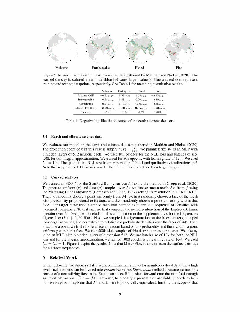
Figure 5: Moser Flow trained on earth sciences data gathered by Mathieu and Nickel (2020). Thelearned density is colored green-blue (blue indicates larger values); Blue and red dots representtraining and testing datapoints, respectively. See Table 1 for matching quantitative results.

Volcano Earthquake Flood FireMixture vMF −0.31±0.07 0.59±0.01 1.09±0.01 −0.23±0.02

Stereographic −0.64±0.20 0.43±0.04 0.99±0.04 −0.40±0.06

Riemannian −0.97±0.15 0.19±0.04 0.90±0.03 −0.66±0.05

Moser Flow (MF) −2.02±0.42 −0.09±0.02 0.62±0.04 −1.03±0.03

Data size 829 6124 4877 12810

Table 1: Negative log-likelihood scores of the earth sciences datasets.

5.4 Earth and climate science data

We evaluate our model on the earth and climate datasets gathered in Mathieu and Nickel (2020).The projection operator π in this case is simply π(x) = x

‖x‖ . We parameterize vθ as an MLP with6 hidden layers of 512 neurons each. We used full batches for the NLL loss and batches of size150k for our integral approximation. We trained for 30k epochs, with learning rate of 1e-4. We usedλ− = 100. The quantitative NLL results are reported in Table 1 and qualitative visualizations in 5.Note that we produce NLL scores smaller than the runner-up method by a large margin.

5.5 Curved surfacesWe trained an SDF f for the Stanford Bunny surfaceM using the method in Gropp et al. (2020).To generate uniform (ν) and data (µ) samples overM we first extract a meshM′ from f usingthe Marching Cubes algorithm (Lorensen and Cline, 1987) setting its resolution to 100x100x100.Then, to randomly choose a point uniformly fromM′ we first randomly choose a face of the meshwith probability proportional to its area, and then randomly choose a point uniformly within thatface. For target µ we used clamped manifold harmonics to create a sequence of densities withincreased complexity. To that end, we first computed the k-th eigenfunction of the Laplace-Beltramioperator overM′ (we provide details on this computation in the supplementary), for the frequencies(eigenvalues) k ∈ {10, 50, 500}. Next, we sampled the eigenfunctions at the faces’ centers, clampedtheir negative values, and normalized to get discrete probability densities over the faces ofM′. Then,to sample a point, we first choose a face at random based on this probability, and then random a pointuniformly within that face. We take 500k i.i.d. samples of this distribution as our dataset. We take vθto be an MLP with 6 hidden layers of dimension 512. We use batch size of 10k for both the NLLloss and for the integral approximation; we ran for 1000 epochs with learning rate of 1e-4. We usedλ− = λ+ = 1. Figure 6 depict the results. Note that Moser Flow is able to learn the surface densitiesfor all three frequencies.

6 Related WorkIn the following, we discuss related work on normalizing flows for manifold-valued data. On a highlevel, such methods can be divided into Parametric versus Riemannian methods. Parametric methodsconsist of a normalizing flow in the Euclidean space Rn, pushed-forward onto the manifold throughan invertible map ψ : Rn → M. However, to globally represent the manifold, ψ needs to be ahomeomorphism implying thatM and Rn are topologically equivalent, limiting the scope of that

9

Frequency k = 10 Frequency k = 50 Frequency k = 500

Figure 6: Moser Flow trained on a curved surface (Stanford Bunny). We show three differenttarget distribution with increasing frequencies, where for each frequency we depict (clockwise fromtop-left): target density, data samples, generated samples, and learned density.

approach. Existing methods in this class are often based on the exponential map expx : TxM ∼=Rn → M of a manifold. This leads to the so called wrapped distributions. This approach hasbeen taken, for instance, by Falorsi et al. (2019) and Bose et al. (2020) to parametrize probabilitydistributions on Lie groups and hyperbolic space. However, Parametric methods based on theexponential map often lead to numerical and computational challenges. For instance, in compactmanifolds (e.g., spheres or the SO(3) group) computing the density of wrapped distributions requiresan infinite summation. On the hyperboloid, on the other hand, the exponential map is numerically notwell-behaved far away from the origin (Dooley and Wildberger, 1993; Al-Mohy and Higham, 2010).

In contrast to Parametric methods, Riemannian methods operate directly on the manifold itself and,as such, avoid numerical instabilities that arise from the mapping onto the manifold. Early workin this class of models proposed transformations along geodesics on the hypersphere by evaluatingthe exponential map at the gradient of a scalar manifold function (Sei, 2011). Rezende et al. (2020)introduced discrete Riemannian flows for hyperspheres and torii based on Möbius transformationsand spherical splines. Mathieu and Nickel (2020) introduced continuous flows on general Riemannianmanifolds (RCNF). In contrast to discrete flows (e.g., Bose et al., 2020; Rezende et al., 2020), suchtime-continuous flows alleviate the previous topological constraints by parametrizing the flow as thesolution to an ODE over the manifold (Grathwohl et al., 2018). Concurrently to RCNF, Lou et al.(2020) and Falorsi and Forré (2020) proposed related extensions of neural ODEs to smooth manifolds.Moser Flow also generates a CNF, however by limiting the flow space (albeit, not the generateddistributions) it allows expressing the learned distribution as the divergence of a vector field.

7 Discussion and limitationsWe introduced Moser Flow, a generative model in the family of CNFs that represents the target densityusing the divergence operator applied to a vector valued neural network. The main benefits of MFstems from the simplicity and locality of the divergence operator. MFs circumvent the need to solvean ODE in the training process, and are thus applicable on a broad class of manifolds. Theoretically,we prove MF is a universal generative model, able to (approximately) generate arbitrary positivetarget densities from arbitrary positive prior densities. Empirically, we show MF enjoys favorablecomputational speed in comparison to previous CNF models, improves density estimation on sphericaldata compared to previous work by a large margin, and for the first time facilitate training a CNFover a general curved surface.

One important future work direction, and a current limitation, is scaling of MF to higher dimensions.This challenge can be roughly broken to three parts: First, the model probabilities µ̄ should becomputed/approximated in log-scale, as probabilities are expected to decrease exponentially withthe dimension. Second, the variance of the numerical approximations of the integral

∫M µ̄−dV

will increase significantly in high dimensions and needs to be controlled. Third, the divergenceterm, div(u), is too costly to be computed exactly in high dimensions and needs to be approximated,similarly to other CNF approaches. Finally, our work suggests a novel generative model, and similarlyto other generative models can be potentially used for generation of fake data and amplify harmfulbiases in the dataset. Mitigating such harms is an active and important area of ongoing research.

10

Acknowledgments

NR is supported by the European Research Council (ERC Consolidator Grant, "LiftMatch" 771136),the Israel Science Foundation (Grant No. 1830/17), and Carolito Stiftung (WAIC).

ReferencesAl-Mohy, A. H. and Higham, N. J. (2010). A New Scaling and Squaring Algorithm for the Matrix

Exponential. SIAM Journal on Matrix Analysis and Applications, 31(3):970–989.

Bose, A. J., Smofsky, A., Liao, R., Panangaden, P., and Hamilton, W. L. (2020). Latent VariableModelling with Hyperbolic Normalizing Flows. arXiv:2002.06336 [cs, stat].

Brown, T. B., Mann, B., Ryder, N., Subbiah, M., Kaplan, J., Dhariwal, P., Neelakantan, A., Shyam,P., Sastry, G., Askell, A., et al. (2020). Language models are few-shot learners. arXiv preprintarXiv:2005.14165.

Chen, M., Tu, B., and Lu, B. (2012). Triangulated manifold meshing method preserving molecularsurface topology. Journal of Molecular Graphics and Modelling, 38:411–418.

Chen, R. T., Rubanova, Y., Bettencourt, J., and Duvenaud, D. (2018). Neural ordinary differentialequations. arXiv preprint arXiv:1806.07366.

Chen, R. T. Q., Behrmann, J., Duvenaud, D., and Jacobsen, J.-H. (2020). Residual flows for invertiblegenerative modeling.

Dacorogna, B. and Moser, J. (1990). On a partial differential equation involving the jacobiandeterminant. In Annales de l’Institut Henri Poincare (C) Non Linear Analysis, volume 7, pages1–26. Elsevier.

Dhariwal, P. and Nichol, A. (2021). Diffusion models beat gans on image synthesis. arXiv preprintarXiv:2105.05233.

Dinh, L., Sohl-Dickstein, J., and Bengio, S. (2016). Density estimation using real nvp. arXiv preprintarXiv:1605.08803.

Dooley, A. and Wildberger, N. (1993). Harmonic analysis and the global exponential map for compactLie groups. Functional Analysis and Its Applications, 27(1):21–27.

Falorsi, L., de Haan, P., Davidson, T. R., and Forré, P. (2019). Reparameterizing Distributions on LieGroups. arXiv:1903.02958 [cs, math, stat].

Falorsi, L. and Forré, P. (2020). Neural Ordinary Differential Equations on Manifolds.arXiv:2006.06663 [cs, stat].

Gerber, S., Tasdizen, T., Fletcher, P. T., Joshi, S., Whitaker, R., Initiative, A. D. N., et al. (2010).Manifold modeling for brain population analysis. Medical image analysis, 14(5):643–653.

Grathwohl, W., Chen, R. T. Q., Bettencourt, J., Sutskever, I., and Duvenaud, D. (2018). Ffjord:Free-form continuous dynamics for scalable reversible generative models.

Gropp, A., Yariv, L., Haim, N., Atzmon, M., and Lipman, Y. (2020). Implicit geometric regularizationfor learning shapes.

Hoppe, H., DeRose, T., Duchamp, T., McDonald, J., and Stuetzle, W. (1992). Surface reconstructionfrom unorganized points. In Proceedings of the 19th annual conference on computer graphics andinteractive techniques, pages 71–78.

Huang, C.-W., Chen, R. T. Q., Tsirigotis, C., and Courville, A. (2021). Convex potential flows:Universal probability distributions with optimal transport and convex optimization.

Kazhdan, M., Bolitho, M., and Hoppe, H. (2006). Poisson surface reconstruction. In Proceedings ofthe fourth Eurographics symposium on Geometry processing, volume 7.

11

Kingma, D. P. and Ba, J. (2014). Adam: A method for stochastic optimization. arXiv preprintarXiv:1412.6980.

Kumar, M., Babaeizadeh, M., Erhan, D., Finn, C., Levine, S., Dinh, L., and Kingma, D. (2019).Videoflow: A flow-based generative model for video. arXiv preprint arXiv:1903.01434, 2(5).

Lee, J. M. (2013). Smooth manifolds. In Introduction to Smooth Manifolds, pages 1–31. Springer.

Lorensen, W. E. and Cline, H. E. (1987). Marching cubes: A high resolution 3d surface constructionalgorithm. ACM siggraph computer graphics, 21(4):163–169.

Lou, A., Lim, D., Katsman, I., Huang, L., Jiang, Q., Lim, S.-N., and De Sa, C. (2020). Neuralmanifold ordinary differential equations.

Mathieu, E. and Nickel, M. (2020). Riemannian continuous normalizing flows. arXiv preprintarXiv:2006.10605.

Moser, J. (1965). On the volume elements on a manifold. Transactions of the American MathematicalSociety, 120(2):286–294.

Papamakarios, G., Nalisnick, E., Rezende, D. J., Mohamed, S., and Lakshminarayanan, B. (2019).Normalizing flows for probabilistic modeling and inference. arXiv preprint arXiv:1912.02762.

Rezende, D. and Mohamed, S. (2015). Variational inference with normalizing flows. In InternationalConference on Machine Learning, pages 1530–1538. PMLR.

Rezende, D. J., Papamakarios, G., Racaniere, S., Albergo, M., Kanwar, G., Shanahan, P., andCranmer, K. (2020). Normalizing flows on tori and spheres. In International Conference onMachine Learning, pages 8083–8092. PMLR.

Sei, T. (2011). A Jacobian Inequality for Gradient Maps on the Sphere and Its Application toDirectional Statistics. Communications in Statistics - Theory and Methods, 42(14):2525–2542.

Tancik, M., Srinivasan, P. P., Mildenhall, B., Fridovich-Keil, S., Raghavan, N., Singhal, U., Ra-mamoorthi, R., Barron, J. T., and Ng, R. (2020). Fourier features let networks learn high frequencyfunctions in low dimensional domains.

12