NOVEMBER 2010

MORTALITY AND MACROECONOMIC FLUCTUATIONS

IN CONTEMPORARY SWEDEN1

Joseacute A Tapia Granados2 and Edward L Ionides

3

Abstract mdash Recent research has provided strong evidence that in the United States in particular and in high- or

middle-income economies in general mortality tends to evolve better in recessions than in expansions It has

been suggested that Sweden may be an exception to this pattern The present investigation shows however that

in the period 1968ndash2003 mortality oscillated procyclically in Sweden deviating from its trend upward during

expansions and downward during recessions This pattern is evidenced by the oscillations of life expectancy total

mortality and age- and sex-specific mortality rates at the national level and also by regional mortality rates for

the major demographic groups during recent decades Results are robust for different economic indicators

methods of detrending and models In lag regression models macroeconomic effects on annual mortality tend to

appear lagged one year As in other countries traffic mortality rises in expansions and declines in recessions and

the same is found for total cardiovascular mortality However macroeconomic effects on ischemic heart disease

mortality appearing at lag two are hard to interpret Reasons for the procyclical oscillations of mortality for in-

consistent results found in previous studies as well as for the differences observed between Sweden and the

United States are discussed

1 Introduction

In a number of countries and periods it has been found that over and above long-term de-

clining trends mortality rates tend to rise in expansions and decline in recessions The main

finding of the present investigation is that the same happened in Sweden in the last three

decades of the 20th century Since mortality oscillates procyclically life expectancy at birth

(e0) oscillates countercyclically and the annual gain in e0 is greater in years of economic

downturn than in years of economic expansion This procyclical oscillation of mortality is

shown in the present study using various statistical models for a range of different mortality

1 This is an expanded version including a number of references figures and appendices that were supressed in

the published version of the paper

2 Social Environment amp Health (SEHSRC) Program Institute for Social Research University of Michigan

Ann Arbor E-mail jatapiaumichedu

3 Department of Statistics University of Michigan Ann Arbor

2 rates and business-cycle indicators These results adds to an emerging consensus that eco-

nomic expansions rather than recessions have harmful effects for health

The next two sections review previous work on mortality and the business cycle and po-

tential pathways linking the economy with mortality Sections 4 and 5 show the data and

methods we have used for the investigation and the results of our analyses The last two sec-

tions include a discussion of the results of other investigations and a general discussion of

our findings in the context of previous work In two appendices we have discussed statistical

issues that are probably beyond the interest of the average reader of this paper

2 Previous Research on Mortality and the Business Cycle

The relation between mortality and the business cycle was already investigated in the 1920s

by Ogburn and Thomas who were surprised by finding a procyclical fluctuation of mortality

in the United States and Britain during the business cycles preceding World War I (Ogburn

1964 Ogburn and Thomas 1922 Thomas 1927) These early studies were largely forgotten

for most of the 20th century probably because the idea that mortality evolves better during

recessions than during expansions was too counterintuitive to be easily accepted

The notion that economic hardship must be bad for health and therefore associated with

higher mortality is deeply ingrained in social science Many investigations in the fields of

public health demography and economics have shown that low income is systematically

associated with higher death rates (Isaacs and Schroeder 2005) Increasing mortality result-

ing from a worsening standard of living is the basis of Malthusrsquos ldquopositive checkrdquo to popula-

tion growth which is a frequent working hypothesis in demography and economic history

(Bengtsson and Saito 2000 Bengtsson et al 2004) Historical studies of preindustrial socie-

ties have indeed shown that mortality upswings are associated for instance with bad har-

vests increases in grain prices or cold winters (Lee 1981 Schofield 1985 Thomas 1941 Livi-

Bacci 1991) However this link between mortality and food price inflation or bad harvests is

considerably weakened with advances in economic development and industrialization (Gal-

loway 1988) In Sweden for example the strong mortality responses to bad harvests ob-

3 served in the 18th century and first half of the 19th century (Fridlizius 1979) disappeared

during the last decades of the 19th century (Thomas 1941 Tapia Granados and Ionides

2008)

In the 1970s and 1980s Brenner repeatedly reported harmful effects of recessions on

mortality other health indicators and social conditions (Brenner 1971 1979 1982 1987)

Brenner utilized relatively unconventional econometric techniques such as Fourier analysis

distributed lag regressions and ARIMA models These studies mostly published in health

journals raised protracted controversy While the results of a few investigations apparently

supported Brenners argument to some extent (Bunn 1979 1980 Junankar 1991 McAv-

inchey 1984) other researchers criticized Brennerrsquos studies for deficient presentation of data

and methods use of lags arbitrarily chosen lack of statistical power with the number of ob-

servations being often close to that of covariates improper methods of detrending and in-

clusion of multiple covariates implying strong collinearity (Eyer 1976a 1976b 1977a Kasl

1979 Gravelle Hutchinson and Stern 1981 Forbes and McGregor 1984 Lew 1979 Winter

1983 Soslashgaard 1992 Wagstaff 1985) Meanwhile with straightforward statistical methods

Eyer (1977b) Higgs (1979) and Graham et al (1992) again found a procyclical fluctuation of

mortality in the United States

In recent years a number of publications have reexamined whether macroeconomic fluc-

tuations are related to short-term oscillations in mortality In a ground-breaking study

Ruhm (2000) applied panel regressions to data from the 50 states of the United States dur-

ing the years 1972ndash1991 showing that beyond long-term trends periods of expanding eco-

nomic activitymdashgauged by low state unemployment levelsmdashwere associated with increased

mortality that is to say that mortality oscillates procyclically Other work using panel re-

gressions has shown that the 1981ndash1982 recession induced substantial reductions of atmos-

pheric pollution associated with significant drops in infant mortality (Chay and Greenstone

2003) that babies born during recessions in the United States have a reduced incidence of

low birth weight and lower infant mortality (Dehejia and Lleras-Muney 2004) and that

death rates oscillate procyclically in Japan (Tapia Granados 2008) the 16 German states

4 (Neumayer 2004) the 50 Spanish provinces (Tapia Granados 2005a) the 96 French deacute-

partements (Buchmueller at al 2007) and the 23 OECD countries (Johansson 2004 Gerd-

tham and Ruhm 2006) The procyclical oscillations of mortality in the United States have

also been confirmed using time-series analyses (Laporte 2004 Tapia Granados 2005b) and

individual-level data from the National Longitudinal Mortality Study (Edwards 2008) The

evolution of mortality rates and life expectancy in the United States during the 1920s and

1930s shows that mortality-based health indicators evolved better during the Great Depres-

sion of 1929-1933 than during the economic expansions of the ldquoroaringrdquo twenties and mid-

thirties (Tapia Granados and Diez Roux 2009) In medium-income market economies mor-

tality responses to macroeconomic downturns have been found to be erratic (Tapinos et al

1997) or even clearly procyclical (Abdala et al 2000 Khang et al 2005 Tapia Granados

2006 Gonzaacutelez and Quast 2010)

Sweden has been the focus of four recent studies by Gerdtham and Johannesson (2005)

Tapia Granados and Ionides (2008) and Svensson (2007 2010) which provide conflicting

evidence on the relation between macroeconomic fluctuations and mortality in that country

The existence and nature of this relation in Sweden seems important because (a) Sweden is a

world leader in health indicators and levels of income per capita (b) the Swedish welfare

state is one of the most developed in the world with universal health care and generous in-

come support for unemployed people provided by the State and (c) the Swedish economy

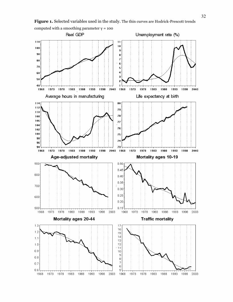
went through major fluctuations in the last decades of the 20th century (see for instance the

wide fluctuations of unemployment figure 1)

The study by Gerdtham and Johannesson (2005) used a sample of 47484 adults inter-

viewed in Sweden in 1980ndash1996 and followed through the end of 1996 for a total of 6571

deaths Using a probit model Gerdtham and Johannesson modeled the probability of death

as a function of age the state of the economy (proxied by a business-cycle indicator) and a

linear trend They found mortality increasing during economic downturns and decreasing in

upturnsmdashie a countercyclical fluctuation of mortalitymdashthough only for male mortality and

only for four business-cycle indicators (notification rate capacity utilization confidence in-

5 dicator and GDP growth) out of six that they considered (the aforementioned plus unem-

ployment and GDP deviation from trend)

Tapia Granados and Ionides (2008) investigated the relation between economic growth

and health progress in Sweden during the 19th and 20th centuries They found that annual

economic growth was positively associated with mortality decline throughout the 19th cen-

tury though the relation became weaker as time passed and was reversed in the second half

of the 20th century during which higher economic growth was associated with lower drops

in mortality While the economy-related effect on health occurs mostly at lag zero in the 19th

century the effect is lagged up to two years in the 20th century These results implying a pro-

cyclical fluctuation of mortality rates after 1950 were found to be robust across a variety of

mortality rates (sex- age- and age- and-sex-specific) statistical procedures (including linear

regression spectral analysis and lag regression models) and economic indicators (GDP per

capita growth unemployment and some measures of inflation) This study did not investi-

gate effects for periods shorter than a half century or for cause-specific mortality but its re-

sults indicate that macroeconomic changes (indexed by annual GDP growth or the annual

change in unemployment) have a lagged effect on the annual change in mortality mostly at

lag one

In two different studies Svensson (2007 2010) has employed panel regressions to analyze

annual rates of mortality and unemployment in the 21 Swedish regions during 1976ndash2005

He could not detect any relation between mortality (neither total nor sex-specific) and un-

employment that was robust to different specifications including year-fixed effects region-

specific linear trends or other methods to avoid potential bias Therefore he was unable to

replicate the countercyclical oscillation of male mortality reported by Gerdtham and Johan-

nesson (though Svensson downplays this inconsistency between his results and those of

Gerdtham and Johannesson) The only robust procyclical oscillation found by Svensson is

for mortality due to work-related injuries which increase in expansions Other cause-

specific mortality rates were found to be procyclical or countercyclical depending on the

specification Svensson found ischemic heart disease mortality to be consistently counter-

6 cyclical though only among those aged 20 to 49 and at the 01 level of statistical signifi-

cance

3 Pathways Linking the Economy and Mortality

Potential pathways leading to a procyclical fluctuation of mortality (figure 2) have been ex-

tensively discussed elsewhere (Ruhm 2000 2004 2005a Tapia Granados 2005a Eyer

1984 Neumayer 2004) They will only be briefly summarized here

Mortality caused by diseases of the circulatory system that is cardiovascular disease

(CVD) mortality is usually the main component of total mortality in most countries It has

been hypothesized that procyclical oscillations of CVD mortality may result from a variety of

CVD risk factors that increase during expansions (Eyer 1977b Ruhm 2000 2005b Tapia

Granados 2005b 2008) These would include stress in the working environmentmdashbecause

of overtime and increased rhythm of work (Sokejima and Kagamimori 1998)mdash reduced

sleep time (Biddle and Hamermesh 1990) atmospheric pollution smoking and consump-

tion of saturated fat and alcohol (Ruhm 2005c) Many of these factors might increase the

risk of death of persons who had a previously developed chronic disease such as cancer

diabetes a respiratory illness or a chronic infection The increase in traffic deaths during

economic booms and the decrease in recessions is a robust finding across countries (Eyer

1977b Ruhm 2000 Neumayer 2004 Tapia Granados 2005a 2005b Khang et al 2005)

The strong procyclical fluctuation of traffic-related injuries and deaths is intuitively ex-

plained by the fact that commuting commercial and recreational traffic rapidly expand in

economic upswings (Baker et al 1984 Ruhm 2000) and the effect is probably aggravated by

the procyclical change in alcohol consumption and by sleep deprivation in expansionary pe-

riods in which overwork is frequent (Biddle and Hamermesh 1990 Liu et al 2002)

Increased infant mortality in expansions has been related to economic activity through

atmospheric pollution (Chay and Greenstone 2003) and healthier behaviors of pregnant

women during recessions (Dehejia and Lleras-Muney 2004) In addition in high-income

economies injury deaths are a quite large proportion of the small annual number of infant

7 and children deaths Thus in this context economic expansions could be associated to an

above-trend level of infant and child mortality through car crashes as well as domestic or

school injuries related to overworked parents or caretakers

4 Data and Methods

In the present investigation crude and sex- and age-specific mortality rates were computed

from deaths and population in five-year age strata taken from Statistics Sweden (2005)

Data on annual unemployment rates real GDP industrial production and the confidence

indicator for the manufacturing industry were obtained from the same source Infant mor-

tality and age-standardized mortality rates were taken from the WHO-HFA (2005) data-

base4 Four indices of Swedish manufacturing activity (average hours aggregate hours

manufacturing output and manufacturing employment) were obtained from the US Bureau

of Labor Statistics (2005) Data on life expectancy at birth are from the Human Mortality

Database (2005)

Our main analysis employs data from Swedish annual statistics (figure 1) from 1968 to

the early 2000s (usually until 2003 with n equal to 35 or 36 in most series) This time frame

was chosen for two reasons first because it is possible that the relation between macroeco-

nomic changes and health progress changed over time and the focus of this investigation is

contemporary Sweden second because a number of cause-specific and agendashadjusted mor-

tality rates for Sweden are available from the WHO Health-For-All database beginning in

1968 or 1970 The reference chronology of the Organisation for Economic Cooperation and

Development (OECD 2006) indicates that there were 10 business cycle troughs in Sweden

(figure 1) between 1968 and 2003

4 In the HFA database age-standardized rates are computed with the direct method applying age-

specific rates for 5-year age-strata (0-4 5-9 etc) to a standard European population For instance

the standardized rate of cancer mortality at ages 0-64 represents what the age-specific rate at ages 0-

64 would have been if the Swedish population aged 0-64 had the same age distribution as the stan-

dard European population

8 Population health is indexed by life expectancy at birth (e0 ldquolife expectancyrdquo for brevity)

and a variety of age- sex- and cause-specific mortality rates Since life expectancy is the best

mortality-based summary index of population health unaffected by the age structure of the

population and allowing intertemporal and cross-sectional comparisons (Shryrock et al

1973) we based many of our analysis in ∆e0 the annual gain in life expectancy as a major

indicator of health progress

Analyses in this paper are either (a) simple correlation models between health and eco-

nomic indicators or (b) lag regressions in which a health indicator is regressed on contem-

poraneous and lagged values of an economic indicator Strong collinearity between business

cycle indicators precludes using combinations of these indicators in the same multivariate

regression model Since both the indicators of population health and the economic indica-

tors used in the study have obvious trends (figure 1) all variables were detrended before

analysis to produce trend-stationary series Several procedures to detrend variables were

used only results obtained either with ldquoHP detrendedrdquo series (ie series obtained by sub-

tracting the trend computed with the Hodrick-Prescott filter5 from the actual value of the

variable) or with variables transformed into first differences (∆xt = xt ndash xt-1) or rate of change

(∆xtxt-1) are presented Other detrending procedures6 were employed in sensitivity analyses

and yielded similar results

Macroeconomic fluctuations are not easy to identify and delimit and not all the different

business cycle indicators gauge them in the same way (Mitchell 1951 Backus et al 1992

Baxter and King 1999) In the present study eight economic indicators were used GDP the

unemployment rate the index of industrial production the confidence indicator and four

indices of activity in manufacturing average working hours aggregate hours output and

employment All of them show significantly correlated fluctuations except the confidence

indicator which fluctuates without a definite relation to the others For the sake of brevity

5 We used a smoothing parameter γ = 100 (figure 1) as advised for annual data (Backus and Kehoe

1992) Appendix A defends this option

6 We used the HP filter applied with γ = 10 and the band-pass filter BP(28) recommended by Baxter and King (1999)

9 results for only three business cycle indicatorsmdashreal GDP the unemployment rate and the

index of average working hours in manufacturingmdashwill be presented here At lag zero de-

trended unemployment and GDP have a strong negative correlation in this Swedish sample

(ndash 075 when both series are in rate of change ndash 085 when both are detrended with the

Hodrick-Prescott filter for both correlations P lt 0001) The index of average hours worked

in manufacturing correlates positively and significantly with unemployment (040 P = 001

both series HP-detrended) at lag zero Therefore both unemployment and average hours are

countercyclical while GDP is procyclical7

Cross-correlations and distributed lag regression models were used to ascertain the con-

comitant variation between ldquohealthrdquo and ldquothe economyrdquo or the coincident or lagged effect of

the latter on the former Cross-correlations between detrended series have been used to ana-

lyze the historical properties of business cycle indicators (Galbraith and Thomas 1941

Backus and Kehoe 1992) biological and medical data (Diggle 1990) and time-series ex-

periments (Glass et al 1975) Distributed lag regressions are a common tool in econometrics

For the sake of consistency the two variables correlated or used as outcome and explanatory

variables in a regression were always detrended by the same method8 In lag regressions we

used the Akaike information criterions (AIC) as an objective approach to choose among the

multiple models that we investigated Although AIC has its strengths and flaws relative to

other model selection criteria such as BIC and adjusted R2 (Claeskens 2008) to minimize

AIC is a common and generally accepted procedure to choose ldquothe bestrdquo model among mod-

els with different lags

7 Business cycle data for the United States and other industrialized countries show average working

hours in manufacturing as a procyclical indicator in Sweden however its strong positive correlation

with unemployment shows that it is clearly a countercyclical one We comment on the potential

causes of this difference in the general discussion section

8 In fact there is an exception to this rule because in some models first differences in e0 or mortality

are regressed on the rate of growth of GDP GDP growth is a major dynamic index of business condi-

tions and moreover because of the exponential growth of real GDP first differences tend to present

exploding heteroskedasticity when the series exceeds a few observations

10 In supplementary analyses utilizing panel regression models we also analyzed Swed-

ish mortality rates and unemployment rates for the 21 Swedish regions in the years 1976ndash

2005 These data were kindly shared with us by Mikael Svensson and correspond to the

data used in his two papers (Svensson 2007 and 2010) We obtained the population data for

the regional analysis from Statistics Sweden

5 Results

51 Correlation Models

For the whole population and for large age groups and with series HP-detrended mortality

has positive correlations with GDP and negative correlations with unemployment and aver-

age hours (table 1) Life expectancy at birth e0 follows the same pattern with reversed signs

as is to be expected if mortality is procyclical9 Out of 54 correlations of detrended economic

indicators with detrended health indicators (table 1) only four correlations have a sign that

is inconsistent with a procyclical oscillation of mortality

When age- and sex-specific mortality rates are correlated with the economic indicators

with variables either HP-detrended (table 2 bottom panel) or in rate of change (table 2 top

panel) the correlations of the HP-detrended variables with the economic indicators are

much stronger However the direction of the correlations is consistently similar in analyses

involving rate of change or HP-detrended series suggesting that the HP-filtering is not in-

troducing spurious results in terms of the sign or direction of correlations with mortality

rates Leaving aside the correlations that are statistically indistinguishable from zero almost

without exception the correlations of age- and sex-specific mortality rates with unemploy-

ment and average hours are negative while the correlations of mortality rates with GDP are

positive (table 2) As observed for larger demographic groups (table 1) the pattern of signs

in the correlations of age-and sex-specific mortality rates (table 2) indicate a procyclical os-

9 The other three manufacturing indicators (aggregate hours output and employment) and the index

of industrial production correlate similarly with mortality and e0 The confidence indicator has erratic

correlations with both the other business cycle indicators and with the health indicators

11 cillation of mortality for most age groups The high correlations between detrended busi-

ness cycle indicators and detrended mortality for ages 10ndash19 and 20ndash44 are apparent in the

fluctuations of these death rates following the swings of the economy (figure 3)

During the period of the study the unemployment rate oscillated very moderately in

Sweden before 1990 never exceeding 3 but in the early 1990s unemployment rose to

around 10 remaining there for most of the decade (figure 1) Correlations between mortal-

ity rates and economic indicators computed in split samples corresponding to the years in

which unemployment was low (1968ndash1989) or high (1989ndash2003) reveal that the results are

quite robust (table 3) In split samples the correlations of life expectancy and mortality rates

with the countercyclical unemployment and average hours and with the procyclical GDP all

show an increase in death rates during expansions However with smaller samples fewer

results are significant and in some cases even coefficient signs are unstable

The zero-lag correlations of detrended series of cause-specific mortality with detrended

economic indicators (table 4) indicate a strong procyclical oscillation of traffic mortality

which shows strong positive correlations with GDP and strong negative correlations with

unemployment and average hours CVD mortality does not reveal any clear relation with

business fluctuations at lag zero One of its components ischemic heart disease mortality or

ldquoheart attacksrdquomdashcausing about one half of total CVD deathsmdash correlates negatively with GDP

(ndash 029) and positively (028) with unemployment at marginal or not significant levels

when considering all ages However at ages over 64 the correlations have the same sign but

they are much stronger all of which suggests that ischemic heart disease at advanced ages

fluctuates countercyclically in Sweden when considering lag zero effects only Cerebrovas-

cular disease (stroke) mortality comprises about one fifth of all CVD deaths and does not re-

veal any definite relation with business cycle indicators at lag zero10

10 Table 4 and other tables omit the results for cancer respiratory disease infectious disease flu

suicide and homicide causes for which we could not find a conclusive relation with macro-economic

fluctuations

12 52 Lag Regression Models

We explored the joint effect on health of coincidental and lagged changes in the economy

with models of the type sum = minus+=p

i itit xH0βα including p lags in which Ht is a health indica-

tor at year t and xtndashi is an economic indicator at year t ndash i In these models health is indexed

by e0 or an age-specific mortality rate and the explanatory variable is either unemployment

GDP or average hours in manufacturing Variables are detrended by conversion either in

first differences or in rate of change In general in models using different methods of de-

trending the estimated effects were consistent in sign For a variety of health indicators we

explored models in which the economy is indexed by an indicator (GDP unemployment or

average hours) including several lags (table 5) For life expectancy crude mortality or age-

specific mortality for large age-groups (table 5) AIC values indicate that models including a

coincidental effect at lag zero and a lagged effect at lag one are to be preferred when the eco-

nomic indicator used as regressor is GDP growth or the change in unemployment However

when the regressor is average hours the models including lag zero only are those that mini-

mize AIC All these distributed lag models in which either GDP or unemployment is the eco-

nomic covariate (table 5 panels A and B) show a significant effect on health at lag one but

when the economic indicator is average hours the effect is at lag zero GDP growth has a sig-

nificant negative effect on life expectancy while unemployment and average hours have sig-

nificant positive effects Similar patterns are observed for crude mortality or mortality for

specific ages Interpreting the sign of the net effect most of these models suggest procyclical

mortality but considering the size of the net effect (adding up effects at lags zero and one)

only the model for mortality at ages 45-64 regressed on GDP growth (table 5 panel A)

reaches marginal significance (the net effect is 0003 + 0022 = 0025 has an standard error

SE = 0013 P = 009) Models with average hours as economic indicator (table 5 panel C)

only require one lag and they suggest procyclical mortality when the economic indicator is

either life expectancy crude mortality or mortality at ages 45-64

13 In these regression models (table 5) the Durbin-Watson d is usually either close to 20

or above 20 Since d = 2 [1 ndash r] where r is the estimated autocorrelation d gt 2 implies evi-

dence against positive autocorrelation of the residuals which would result in underestimates

of standard errors and spurious significance 11

We also examined some models in which an age-standardized mortality rate is regressed

on coincidental or lagged GDP growth (table 6) For all-cause mortality sex-specific age-

adjusted mortality for both males and females and sex-specific age-adjusted mortality in

ages 25ndash64 (table 6 panel A) the specification minimizing AIC is the one including effects

at lags zero and one With only a few exceptions in which lag-two effects are also needed this

is also true for CVD mortality in different demographic groups (table 6 panel B) However

for traffic mortality (table 6 panel B bottom) the minimization of AIC occurs in specifica-

tions including just lag-zero effects

For total mortality male mortality and female mortality and for male mortality at ages

25-64 predominantly positive and statistically significant effects of GDP growth on mortality

at lag one indicate a procyclical oscillation of mortality rates For CVD mortality at all ages

and ages below 65 positive (and significant) effects of GDP growth at lag one also indicate a

procyclical oscillation of this type of mortality However for CVD mortality at ages 65 and

over what predominates is negative effects of GDP growth (at lags zero and two)

In regressions modeling coincidental and lagged effects of GDP growth on ischemic heart

disease mortality (table 6 panel B) almost without exception there are negative effects at lag

zero and positive effects at lag one and the positive effects at lag one are often statistically

significant and predominant However for ischemic heart disease mortality in males the

11 In only a few cases d is large enough to suggest negative autocorrelation (see footnote in table 5)

Adjusting for autocorrelation of the residuals did as expected produce similar parameter estimates

with some additional statistical significance To avoid the need to justify selection of a specific autocor-

related model we simply present the conservative unadjusted values For further discussion of these

issues see appendix B

14 model minimizing AIC also includes effects at lag two and the net effect of GDP growth on

this type of mortality in males is negative ie ischemic heart disease mortality decreases

with greater GDP growth Overall this indicates a countercyclical oscillation of ischemic

heart disease mortality However the effects at lag two are difficult to interpret Business

cycles over recent decades in Sweden last approximately 4 years (according to the OECD

chronology the mean + SD of the trough-to-trough distance is 38 + 14 years) This implies

that an effect of high GDP growth lagged two years will likely occur actually when GDP

growth is already low in the next phase of the cycle For ischemic heart disease at ages 85

and over there are negative effects at lags zero and two and a significant positive effect at lag

one so that the net effect of GDP growth is negative the positive effect for lag one is statisti-

cally significant but the net effect is not

Overall considering lag regression models (tables 5 and 6) and correlations (tables 1 to 4)

for the period 1968-2003 the results are consistent for major health indicators Results for

life expectancy total mortality and crude or age-adjusted total mortality in large age groups

indicate a procyclical fluctuation of death rates for the whole population and for both males

and females Less consistent are the correlations and regression results for age-specific mor-

tality rates The link between economic expansions (recessions) and increases (falls) in mor-

tality rates seems to be stronger in adolescents young adults and adults of middle age In-

fant mortality also fluctuates procyclically Results for ages 65-84 or over 65 are equivocal

and for mortality at ages 85 and over we could not find any statistically significant evidence

of a link with business cycle fluctuations

53 Size of the Effect

The net effects of GDP growth at lags zero) and lag one (ndash 097 +335 = 232) on total age-

adjusted mortality measured per 100000 population (table 6 panel A) imply that each extra

percentage point in GDP growth will increase mortality in about 232 deaths per 100000 In

recent years the age-standardized death rate is 600 per 100000 Since the Swedish popula-

tion is about 9 million each percentage point increase in GDP growth would cause

15 [232105] middot 9 106 = 209 extra deaths or an increase of a slightly less than half a percent

(232600 = 04) in age-adjusted mortality During the period of study GDP growth oscil-

lated between ndash2 in major downturns and 6 in major expansions Therefore a typical

expansion in which GDP growth increases three or four percentage points would increase

age-adjusted mortality between one and two percentage points with an additional death toll

of 600 to 800 fatalities

Modeling the relation between macroeconomic change and health using the annual varia-

tions in unemployment (∆Ut ) and life expectancy (∆e0 t) the estimated equation (error term

omitted) is

∆e0t = 0164 ndash 0026 middot ∆Ut + 0076 middot ∆Ut -1 (this is model [6] in table 5) It implies a gain of 0164 years in life expectancy from time t-1

to time t after no change in unemployment from time t-2 to time t-1 and from time t-1 to

time t (that it ∆Ut = ∆Ut -1 = 0) On the other hand the gain in life expectancy will be zero

(∆e0 t = 0) with two successive equal drops in annual unemployment of 33 percentage

pointsmdashwhich in macroeconomic terms means a brisk economic expansionmdashwhile greater

annual drops in unemployment will reduce life expectancy A recession in which unemploy-

ment grows 2 percentage points for two consecutive years (∆Ut = ∆Ut-1 = 2) will be associated

with an annual increase of 0264 years in life expectancy a gain 23 times greater than the

0114 years gained in an expansion during which the unemployment rate consecutively drops

one percentage point per year (∆Ut = ∆Ut-1 = ndash1) For reference it is important to note that

during the period included in this investigation life expectancy at birth increased about 5

years during three decades for an annual gain of 018 years while the unemployment rate

never increased more than 38 percentage point or dropped more than 13 points per year

6 Results of Other Investigations on Sweden

The sample in Gerdtham and Johannessonrsquos study is very large including over 500000 per-

son-year observations (Gerdtham and Johannesson 2005 p 205) However their analysis

only includes 6571 deaths occurring over 16 years while our analyses include all deaths that

16 occurred in Sweden for each year of the study period ie over 90000 deaths per year for

a total of over 3 million deaths during 1968-2002 National death rates give greater statisti-

cal power than a sample of 6571 deaths to investigate various model specifications and par-

ticularly to check model consistency across population subgroups The sample size limita-

tions in the analyses reported by Gerdtham and Johannesson are illustrated for example by

the fact that they had only 43 traffic-related deaths (p 214) which implied that the business-

cycle impact on this cause of death could not be analyzed Moreover though Gerdtham and

Johannesson present some supplementary analyses using education and income as individ-

ual-level covariates the only individual covariate used in their primary analysis is the age at

death We also control for age in our analyses by using the aggregate measures of life expec-

tancy and age-specific mortality rates

According to Gerdtham and Johannesson (p 210) when quadratic and cubic trends were

included in their models some statistically significant results were weakened Since linear

trends may be insufficient to account for the long-term curvilinear trends in indicators of the

Swedish economy in recent decades (figure 1) the imperfect control for these trends may

have produced biased results For instance the enormous size of the effect of macroeco-

nomic change on cancer mortality reported by Gerdtham and Johannesson may imply model

misspecification Similarly their finding that results vary from procyclical to countercyclical

fluctuation of mortality depending on the economic indicator used suggests instability in the

results There are also limitations to the indicators they used For example opinion-based

variables such as the confidence indicator or the notification rate may be very imperfect in-

dicators of the fluctuations of the real economy Indeed we have verified that the confidence

indicator one of the indicators rendering countercyclical results for mortality in Gerdtham

and Johannessonrsquos investigation reveals a very erratic relation with GDP unemployment

and all the other business indicators based on manufacturing and is therefore likely to be a

very unreliable index (neither procyclical nor countercyclical) of the changes in the real

economy

17 Another limitation of Gerdtham and Johannessonrsquos investigation is the short period of

data collection which allows for few recurrent changes in the state of the economy In their

paper they state (p 209) that the relation between unemployment and probability of death is

negative for unemployment (so that mortality is procyclical) over the whole study period

1981ndash1996 but turns positive (counter-cyclical) for male and zero for females in the subpe-

riod 1981ndash1991 Gerdtham and Johannesson consider the procyclical mortality result ob-

tained for the years 1981ndash1996 to be biased by the high unemployment in the 1990s How-

ever if there is a real relation (whether procyclical or countercyclical) between the fluctua-

tions of the economy and the mortality risk the relation will tend to appear most clearly in

samples covering longer periods and will tend to became unstable or to disappear as the ana-

lyzed period gets shorter and closer to the average duration of business cycles This instabil-

ity is shown for instance by our split-sample correlations of HP-detrended unemployment

and mortality at ages 45ndash64 (table 3 in the present paper) The correlation between these

variables is positive (ie a countercyclical fluctuation of mortality) in the years 1981ndash1992

(the sample often used by Gerdtham and Johannesson) though it is negative (suggesting

procyclical mortality) in other split samples (table 3 panel B) and over the whole period

1969ndash2003 (table 1) Business cycles may vary in length ldquofrom more than one year to ten or

twelve yearsrdquomdasha classical definition by Mitchell (1951 p 6) that fits very well with the data

analyzed here with macroeconomic fluctuations on average 4 years long Therefore ten

years may be too short a period to study any business-cycle-related issue Indeed the period

1981ndash1991 that Gerdtham and Johanesson often use to present results is one in which un-

employment changed very little and GDP growth varied within very narrow limits (figure 1)

Observing only part of the full range of variation of a covariate is one of the potential causes

of biased results in any statistical model

Most of the results supporting a countercyclical oscillation of mortality (only for males) in

Gerdtham and Johannessonrsquos investigation come from models in which the only considered

effect of the economy on mortality is a coincidental one As reported by the authors adding

lagged variables with lags up to four years produced procyclical mortality effects at t ndash 1 for

18 both unemployment and GDP deviation from trend However since the coefficients for

the lagged economic indicator in these specifications are not reported by Gerdtham and Jo-

hannesson it is not possible to evaluate the net effect

It is also important to note that a positive impact of GDP growth and a negative impact of

unemployment on the death rate in the next year is consistent with our results and indicates

a procyclical oscillation of mortality

In summary we believe the results of Gerdtham and Johannesson (2005) are much less

reliable than ours because insufficient consideration for lagged effects use of unreliable

business-cycle indicators data collected during a very short period in terms of business cy-

cles and lack of power to detect effects due to few deaths in their sample

We performed some analyses using the Swedish regional data used by Svensson (2007

2010) We reproduced his results in several specifications of panel regressions Then we re-

analyzed this data detrending the mortality and the unemployment regional data by either

subtracting an HP trend (γ = 100) or by converting variables into first differences We inves-

tigated models of the form

ttr

k

i itritr UM ψεβα ++sdot+= sum = minus 0 dd

where dMrt is detrended mortality of region r at year t dUr t-i is detrended unemployment

for region r at year t ndash i εr t is a normally distributed error term and ψt is a normally dis-

tributed random effect for year This random effect (Venables and Ripley 2002) adjusts for

the spatial autocorrelation between regions (Layne 2007) To explore lagged effects we esti-

mated models for k = 0 k = 1 k = 2 k = 3 and for each dependent variable we chose the

model minimizing AIC The best fit in terms of AIC was obtained when the model included

effects at lags zero and one or at lag zero only (table 7) However for some mortality rates

AIC is minimized in specifications including lags zero to two or even lags zero to three This

and the effects with alternating sign that are difficult to explain makes some of these results

puzzling revealing the complexities of interpreting lag regression models At any rate what

these regional models show is that negative and often statistically significant effects of re-

19 gional unemployment predominate at lags zero or one for total mortality and for sex-

specific mortality indicating a procyclical fluctuation of total and sex-specific mortality

With very few qualifications the same can be said for mortality at ages 45ndash64 and 65 and

over as well as traffic mortality However for ischemic heart disease mortality positive ef-

fects that predominate at lags zero and two make the interpretation of these effects equivo-

cal

Considering all the results of regressions with regional data12 we interpret the negative

signs of the predominant effects at lag one as evidence consistent with our analysis of na-

tional data indicating a procyclical oscillation of total male and female mortality as well as

mortality at the three specific ages that Svensson investigated We believe that Svenssons

analysis of regional data missed the procyclical oscillation of death rates primarily because

he did not consider lagged effects In addition his panel methods (including fixed effects for

year and sometimes region-specific linear trends too) could be less statistically powerful

than our random effect specification

7 General Discussion

The procyclical fluctuation of national Swedish mortality rates revealed by the results in ear-

lier sections is consistent with results from other industrialized countries it is based on the

period 1968ndash2003 which included eight or nine macroeconomic fluctuations it is found in

total male and female mortality as well as age-specific mortality for most age groups it is

revealed by the correlations of mortality with seven economic indicators and also by lag

models in which health indicators are regressed on an economic indicator and finally it is

consistent with the procyclical fluctuation of total and age-specific mortality rates (and the

countercyclical fluctuation of life expectancy at birth) found by Tapia Granados and Ionides

(2008) in time series for the second half of the 20th century In contrast the countercyclical

12 In regional panel models not including a random effect for year the unemployment effects were

greater in size and much more significant than those reported in table 7 However we consider them

probably biased by spatial autocorrelation

20 fluctuation of mortality reported by Gerdtham and Johannesson (2005) is inconsistent

with other recent results from industrialized countries is observed only for male mortality

appears only for selected business cycle indicators (some of questionable validity) and is

sensitive to the inclusion of lagged terms in the regressions or to the change in the time

frame considered often appearing only when the time frame is restricted to the expansion-

ary years 1981ndash1991 Moreover with regional data Svensson (2007 2008) was unable to

reproduce Gerdtham and Johannessonrsquos finding of a countercyclical fluctuation of male

mortality while our reanalysis of Svenssonrsquos regional data produced results that are basi-

cally consistent with the other results presented in this paper as well as with the results in

Tapia Granados and Ionides (2008) Considering all the evidence it must be concluded that

in recent decades total mortality in Sweden as well as male and female mortality individu-

ally have oscillated procyclically

CVD is the first cause of death in most countries and in Sweden about half of all death are

attributed to this cause CVD deaths have been found to be strongly procyclical at lag zero in

the United States (Ruhm 2000 Tapia Granados 2005b) Germany (Neumayer 2004) and

the OECD countries as a group (Gerdtham and Ruhm 2006) while in Spain they were found

to be very slightly procyclical (Tapia Granados 2005) In Sweden the lag-zero correlations of

CVD mortality with economic indicators (table 4) do not reveal a comovement of both but

lag regression models indicate a predominantly positive net effect of GDP growth at lags zero

and one on this type of mortality (table 6) Therefore overall CVD mortality in Sweden

tends to rise in expansions procyclically The same pattern is observed for stroke mortality

at all ages or at ages below 65 (table 6 panel B) though for ages 65-74 the preferred model

only includes a positive effect at lag zero what implies a countercyclical oscillation of stroke

mortality at these ages

Findings for ischemic heart disease are much more difficult to interpret When modeled

in lag regressions at the national level (table 6 panel B) ischemic heart disease mortality

reveals predominantly positive effects of GDP at lag one This suggests a procyclical

fluctuation with heart attacks fluctuating upward one year after the start of an expansion

21 and fluctuating downward one year after the start of a recession However in regional

regression models (table 7) positive effects of unemployment at lags zero and two

predominate and cross-correlation analyses of national data also suggest positive effects of

unemployment ie countercyclical effects on ischemic heart disease mortality at ages 65

and over (table 4) But most fatal heart attacks (ie deaths attributed to ischemic heart

disease) occur at advanced age Additional work is needed to better identify the effects of the

economy on ischemic heart disease mortality and why it may oscillate differently than other

causes

In our findings traffic injury mortality correlates strongly with the business cycle at lag

zero (figure 3) particularly at young and middle ages (table 4) Regression models in which

the change in traffic mortality is regressed on coincidental and lagged GDP growth (table 6

panel B bottom) also reveal this procyclical oscillation of traffic mortality at all ages and for

males but at specific ages the regression coefficients are indistinguishable from zero and in

panel models with regional data (table 7) marginally significant effects appear at lag three

Two factors may explain these results First the differencing of a time series converting it

into a rate of change or a first difference series largely filters out the fluctuations in busi-

ness-cycle frequencies This can result in failure to detect relations between variables at the

business-cycle frequencies (Baxter and King 1999) and is one of the reasons for the increas-

ing use of the HP filter and other detrending procedures instead of differencing Second

strong associations at a larger level of aggregation (at all ages or at the national level) may

weaken when mortality is disaggregated (by age strata or by regions) because of the intro-

duction of statistical noise

The strongly procyclical character of CVD mortality in general (Ruhm 2000 Tapia

Granados 2005) and heart attack mortality in the United States for all ages (Ruhm 2008)

contrasts with the absence of a clear procyclical oscillation in ischemic heart disease mortal-

ity reported here and elsewhere (Svensson 2007) for Sweden It has been previously pro-

posed that the Swedish welfare statemdashwith labor regulations and a labor market more

friendly for employees than in the United Statesmdashcould be a factor in explaining a lower im-

22 pact of macroeconomic fluctuations on health in Sweden (Gerdtham and Ruhm 2006

Ruhm 2006 Svensson 2007) and this hypothesis deserves further investigation

It is plausible that differences between institutional regulations of working conditions

and labor markets between Sweden and the United States may perhaps account for the dif-

ferential busyness-cycle dynamics of CVD mortality in both countries The index of average

hours worked in manufacturing has long been considered a leading business cycle indicator

(Mitchell 1951) Early in expansions firms demand overtime from workers and tend to hold

off on hiring additional workers until managers are confident that demand is growing Then

average hours will increase early in an expansion and then will decrease Similarly early in a

recession employers will reduce hours worked to reduce output and costs and average hours

will go down but if the slowdown deepens into a recession layoffs eventually will raise aver-

age hours Differences in the ability of firms to hire and fire workers easily or demand over-

time from employees may well account for the fact that the index of average hours in manu-

facturing is procyclical in the United States and countercyclical in Sweden The countercycli-

cal character of this index if present in other OECD economiesmdashin many European coun-

tries mandatory overtime does not exist and there are generally more limitations for freely

firing workers than in the United States (Chung 2007)mdashmight explain why Johansson

(2004) while getting results indicating an increase of mortality in periods of economic ex-

pansion finds that an increase in hours worked per employed person significantly decreases

the mortality rate in a sample of 23 OECD countries during 1960ndash1997

In this Swedish sample HP-detrended infant mortality significantly correlates negative

with detrended unemployment (tables 1 and 3) and first differences in GDP growth have a

marginally significant positive effect on infant mortality at lag one (table 6) all of which sug-

gest a procyclical oscillation of infant deaths Potential pathways for procyclical infant mor-

tality were mentioned in section 3 On the other hand since traffic-related deaths are in-

tensely procyclical and a major cause of mortality in adolescents and young adults (table 4)

they are a very likely cause of the procyclical oscillation of deaths at ages 10ndash19 (tables 1 and

2)

23 We report only bivariate models Therefore our results can be challenged on the

grounds of potential bias due to omitted variables However results based on the analyses of

economic indicators covering a number of business cycles and converted into stationary se-

ries by filtering or differencing make it very unlikely that omitted variables may significantly

bias the results with respect to business cycle fluctuations Indeed many variables change

together with the levels of economic activity (for instance overtime average levels of daily

sleep volume of road traffic atmospheric pollution etc) and these are exactly the candi-

date intermediary factors connecting ldquothe economyrdquo with the health outcomes It is difficult

to imagine real omitted variables that are not an intrinsic part of the aggregate fluctuations

of economic activity indexed in this study by variables such as unemployment or GDP A

lurking variable seriously biasing the present results might be for instance technological

changes having an immediate or short-lagged contractionary effect on mortality and ap-

pearing or being implemented population-wide late in each expansion or early in each reces-

sion inducing in this way a procyclical oscillation of mortality But this kind of technological

innovation is hard to imagine and it is even harder to believe that it would have such an in-

tense effect on mortality fluctuations (McKinlay et al 1989)

Results of this investigation can also be challenged on the basis of criticisms of methods

of detrending in general the HP filter in particular or the use of γ = 100 when dealing with

annual data (Ashley and Verbrugge 2006 Baxter and King 1999 Dagum and Giannerini

2006) However the HP filter is now a standard method for detrending economic data

(Ravn and Uhlig 2002) and γ = 100 is very regularly used with yearly observations and is

the default value for annual data in econometric software packages Furthermore our overall

conclusions are robust to variations in the choice of γ (for additional discussion of the

choice of γ see Appendix A) Contrary to the view that HP-filtering introduces business-

cycle frequency fluctuations in the data so that the computed correlations between HP-

detrended series are just ldquodiscoveringrdquo a spurious artifactual pulsation introduced by the fil-

ter in this investigation cross-correlations and distributed lag models with variables either

HP-detrended or differenced produced similar qualitative results revealing procyclical oscil-

24 lations of death rates Panel regressions (Neumayer 2004 Ruhm 2000 Ruhm 2005b

Tapia Granados 2005a) and analysis of time series (Laporte 2004 Tapia Granados 2005b)

have produced exactly the same conclusion when they were applied in the past to study the

relation between macroeconomic change and mortality in the United States

Based on the results of a number of statistical models reported here as well as our ex-

amination of the results of other investigations we conclude that in Sweden mortality of

both males and females oscillated procyclically during recent decades Since the long-term

trend of age-adjusted mortality rates is a falling one its procyclical oscillation means that

age-adjusted mortality declines in recessions while during expansions it declines less rap-

idly or even increases The fact that even in a country like Sweden with a highly developed

system of social services and publicly financed health care mortality tends to evolve for the

worse during economic expansions must be a warning call about the unintended conse-

quences of economic growth13 The policy implications of procyclical mortality are too broad

to be discussed here but a clear implication is the need to further study the pathways con-

necting the fluctuations of the economy with the oscillations of death rates Knowledge of

these mechanisms may lead to the development of policies to reduce the harmful effects of

macroeconomic fluctuations on health

13 The potentially harmful consequences of economic growth for social welfare were already discussed

decades ago from a variety of perspectives for instance by Mishan (1970) Hirsch (1976) Daly (1977)

Zolotas (1981) and Eyer (1984) Georgescu-Roegen (1976 1971 Randolph Beard and Lozada 1999)

presented a comprehensive view of the bioenvironmental implications of the exponential growth of

the economy

25 Table 1 Cross-correlations between three economic indicators life expectancy and se-

lected mortality rates for Sweden 1968ndash2003

Health indicator Unemployment GDP Average hours in manufacturing

Life expectancy 035 ndash 015 051

LE males 037 ndash 018 048

LE females 030dagger ndash 010 049

ASMR all ages ndash 027 021 ndash 049

ASMR males ndash 019 012 ndash 037

ASMR females ndash 031dagger 026 ndash 038

Crude mortality rate ndash 024 011 ndash 039

CMR males ndash 017 008 ndash 037

CMR females ndash 027 014 ndash 038

Age-specific mortality rates

Infant mortality ndash 041 024 ndash 016

0ndash4 ndash 048 036 ndash 034

5ndash9 ndash 001 ndash 008 ndash 034

10ndash19 ndash 042 052 ndash 012

20ndash44 ndash 042 036 ndash 021

25ndash64 ndash 030dagger 017 ndash 034

45ndash64 ndash 025 011 ndash 033

55ndash64 ndash 026 007 ndash 042

65ndash84 ndash 003 ndash 013 ndash 037

85 and over 016 ndash019 ndash010

Notes Correlations with mortality rates are based on n = 36 or close to 36 in most cases in life expec-

tancy correlations n = 32 ASMR is age-standardized mortality rate All variables detrended with the

Hodrick-Prescott filter γ = 100

dagger P lt 01 P lt 005 P lt 001

26 Table 2 Cross-correlation between economic indicators and age- and sex-specific mor-

tality rates for large age strata In each of the two panels the series are either in rate of

change or HP-detrended

Age-specific mortality Unemployment rate GDP Average hours in manufacturing

AmdashSeries in rate of change

Male mortality

10ndash19 ndash 009 015 ndash 004

20ndash44 ndash 008 005 ndash 004

45ndash64 ndash 006 011 ndash 056

65ndash84 027 ndash 023 ndash 030dagger

85 amp over 009 ndash 013 ndash008

Female mortality

10ndash19 ndash 016 015 ndash 010

20ndash44 ndash 019 020 ndash 014

45ndash64 ndash 019 024 000

65ndash84 010 ndash 023 ndash 016

85 amp over 018 ndash020 ndash019

BmdashHPndashdetrended series

Male mortality

10ndash19 ndash 041 050 ndash 004

20ndash44 ndash 042 031dagger ndash 017

45ndash64 ndash 014 001 ndash 038

65ndash84 006 ndash 016 ndash 028dagger

85 amp over 021 ndash017 007

Female mortality

10ndash19 ndash 028dagger 034 ndash 020

20ndash44 ndash 030dagger 031dagger ndash 019

45ndash64 ndash 031dagger 020 ndash 015

65ndash84 ndash 011 ndash 008 ndash 040

85 amp over 005 ndash014 ndash 021

dagger P lt 01 P lt 005 P lt 001

27 Table 3 Split sample cross-correlations of economic indicators with selected mortality

rates and life expectancy

Health indicator Unemployment GDP Average hours in manufacturing

A Sample 1968ndash1989 (n = 22) Life expectancy 022 004 038dagger Males 027 006 037dagger Females 016 001 035

Crude mortality rate ndash 016 006 ndash 029

Males ndash 007 001 ndash 023

Females ndash 022 009 ndash 034dagger

Infant mortality 030 ndash 009 046

Mortality 10ndash19 ndash 047 069 016

Mortality 20ndash44 ndash 061 041 ndash 027

Mortality 45ndash64 011 ndash 024 ndash 032

Mortality 65ndash84 007 ndash 018 ndash 032

Mortality 85 amp over 009 ndash 020 ndash 026

B Sample 1989-2003 (n = 15)

Life expectancya 053 ndash 029 073

Malesa 061dagger ndash 039 069

Femalesa 044 ndash 017 074

Crude mortality rate ndash 020 001 ndash 044dagger

Males ndash 010 ndash 008 ndash 045dagger

Females ndash 025 007 ndash 039

Infant mortality ndash 078 051dagger ndash 068

Mortality 10ndash19 ndash 050dagger 046dagger ndash 039

Mortality 20ndash44 ndash 050dagger 047dagger ndash 024

Mortality 45ndash64 ndash 030 018 ndash 022

Mortality 65ndash84 006 ndash 028 ndash 034

Mortality 85 amp over 036 ndash028 012 C Sample 1981ndash1992 (n = 11) Life expectancy 053 040 ndash 037dagger Males 059dagger 049 ndash 033dagger Females 045 030 ndash 040

Crude mortality rate ndash 028 025 ndash 010

Males ndash 018 017 ndash 001

Females ndash 036 031 ndash 017dagger

Infant mortality ndash 041 015 046

Mortality 10ndash19 ndash 082 085 ndash 031

Mortality 20ndash44 ndash 072 082 ndash 011

Mortality 45ndash64 039 ndash 041 015

Mortality 65ndash84 ndash 005 ndash 008 ndash 015

Mortality 85 amp over 021 ndash 027 ndash 018 a n = 9 dagger P lt 01 P lt 005 P lt 001 P lt 0001 Notes All variables detrended with the Hodrick-Prescott filter γ = 100

28

Traffic-related mortality (V01-V99)

a

ndash 067 069 ndash 027

Males ndash 053 058 ndash 021 Females ndash 051 050 ndash 030dagger Ages 15ndash24 ndash 065 068 ndash 010 Ages 25ndash34 ndash 053 039 ndash 046 Ages 35ndash44 ndash 017 019 ndash 012 Ages 45ndash54 ndash 057 060 ndash 025 Ages 55ndash64 ndash 040 041 ndash 029 Ages 65ndash74 ndash 021 024 ndash 002 Ages 75ndash84 ndash 024 025 002

Notes n = 32 or close to 32 for each correlation model Variables detrended with the HP filter γ = 100 Age-standardized

death rates from the WHO-Europe HFA Database

a Codes according to the International Classification of Diseases 10th ed (ICD10)

Table 4 Correlations between economic indicators and cause-specific mortality rates for

the years 1968ndash2002 in Sweden

Mortality rate

Unemploy-ment

GDP

Average hrs in manufacturing

Cardiovascular disease ( I00-I99)a

014 ndash 017 ndash 014

Males 019 ndash 013 ndash 010 Females 006 ndash 011 ndash 016 Ages 55ndash64 males ndash 002 ndash 015 ndash 018 Ages 55ndash64 females ndash 016 006 005 Ages 65ndash74 males 021 ndash 022 ndash 016 Ages 65ndash74 females 013 ndash 015 ndash 017 Ages 75ndash84 001 ndash 009 ndash 015

Ischemic heart disease (I20-I25)a

028dagger ndash 029 ndash 010

Males 027 ndash 028 ndash 003 Females 027 ndash 029 ndash 019 Ages 25ndash64 males 005 ndash 010 ndash 002 Ages 25ndash64 females ndash 037 026 ndash 018 Ages 35ndash44 males 015 ndash 023 009 Ages 35ndash44 females ndash 034 027 ndash 019 Ages 45ndash54 males 011 ndash 005 ndash 002 Ages 45ndash54 females ndash 026 019 ndash 024 Ages 55ndash64 males ndash 001 ndash 007 ndash 004 Ages 55ndash64 females ndash 024 016 ndash 005 Ages 65 and older 033dagger ndash 032dagger ndash 010 Ages 65 and older males 032dagger ndash 029 ndash 004 Ages 65 and older females 033dagger ndash 032 ndash 017 Ages 85 and older 039 ndash 036 000

Cerebrovascular disease (stroke I60-I69)a

ndash 016 013 ndash 018

Ages 25ndash64 ndash 008 003 ndash 017 Ages 25ndash64 males 001 ndash 014 ndash 033 Ages 25ndash64 females 005 003 009 Ages 65ndash74 007 006 ndash 019 Ages 65ndash74 males 021 ndash 022 ndash 016 Ages 65ndash74 females 013 ndash 015 ndash 017

29

Table 5 Parameter estimates in models with a health indicator in first differences regressed on a constant and coincidental and lagged valuesmdashexcept in panel Cmdashof an economic indicator

Explanatory

variable

Dependent

variable

Lag 0

Lag 1

n

d

R2

Model

Interpretation of the net effect

0027 ndash 0041 31 270a 015 [1] Procyclical mortality

(0019) (0019)

Life expec-

tancy

ndash 0039 0048 32 274 014 [2] Procyclical mortality

(0023) (0023)

Crude mor-

tality

0003 0000 35 246 002 [3]

(0003) (0003)

Mortality

ages 20ndash44

0003 0022dagger 35 176 012 [4] Procyclical mortality

(0012) (0012)

Mortality

ages 45ndash64

ndash 0173dagger 0124 35 289 013 [5] Countercyclical mortality

(0085) (0085)

A

Eco

no

mic

gro

wth

(p

erce

nt

rate

of

chan

ge

of

real

GD

P)

Mortality

ages 65ndash84

ndash 0026 0076dagger 30 264 011 [6] Procyclical mortality

(0042) (0043)

Life expec-

tancy

0076 ndash 0119 34 245 015 [7] Procyclical mortality

(0050) (0050)

Crude mor-

tality

ndash 0006 0002 34 255 002 [8]

(0007) (0007)

Mortality

ages 20ndash44

ndash 0018 ndash 0018 34 162 007 [9]

(0025) (0025)

Mortality

ages 45ndash64

0327dagger ndash 0379dagger 34 245 013 [10] Equivocal

B

Un

emp

loy

men

t ra

te

in f

irst

dif

fer-

ence

s

Mortality

ages 65ndash84 (0186) (0187)

0043dagger 31 296a 011 [11] Procyclical mortality

(0023)

Life expec-

tancy

ndash 0059 35 293a 012 [12] Procyclical mortality

(0027)

Crude mor-

tality

ndash 0002 33 243 001 [13]

(0004)

Mortality

ages 20ndash44

ndash 0033 35 211 014 [14] Procyclical mortality

(0014)

Mortality

ages 45ndash64

ndash 0014 35 296a 005 [15]

C

Av

erag

e h

ou

rs i

n m

anu

fact

uri

ng

in f

irst

dif

fere

nce

s

Mortality

ages 65ndash84 (0105)

dagger P lt 01 P lt 005 a P lt 005 for the null hypothesis of no negative autocorrelation of the error term

Notes Standard errors in parentheses Data include years from 1968 to the early 2000s Estimates statistically significant at a

confidence level of 90 or higher are highlighted in boldface Mortality rates are measured in deaths per 1000 population life

expectancy in years In similar models using age-specific mortality for ages 85 and over the lsquobestrsquo model was the one including

just the lag-zero effect but the parameter estimates and its standard errors were approximately of the same sizemdashthat is the

effect was indistinguishable from zeromdash and the R2 was 6 or lower

30

Table 6 Regression estimates of the coincidental and lagged effect of GDP growth on the an-

nual change in age-standardized mortality rates in models minimizing AIC among models in-

cluding just lag zero lags zero and one or lags zero to two

Mortality rate Lag 0 Lag 1 Lag 2

Oscillation of mortality ac-cording to the net effect

A General mortality

All ages ndash 097 335 Procyclical

Males ndash 186 468 Procyclical

Females ndash 036 238 dagger Procyclical

Infant mortality (age lt1) ndash 004 006 dagger Procyclical

Ages 25-64

Males ndash 034 165 Procyclical

Females 105 dagger Procyclical

B Cause-specific mortality

Cardiovascular disease

All ages ndash 145 216 Procyclical

Ages 0-64 ndash 034 056 Procyclical

Ages 45-54 ndash 015 059 Procyclical

Ages 55-64 ndash 167 271 Procyclical

Ages 65-74 ndash 183 Countercyclical

Ages 75-84 ndash 1580 2608 ndash 1385 Equivocal

Ischemic heart disease

All ages ndash 095 165 Procyclical

Males ndash 198 345 ndash 203 Equivocal

Females ndash 069 108 Procyclical

Ages 25-64 ndash 019 062 Procyclical

Males ndash 045 094 dagger Procyclical

Females 007 030 dagger Procyclical

Ages 65+ ndash 770 1196 dagger Procyclical

Ages 85+ ndash 5747 8172 ndash 4704 Equivocal

Cerebrovascular disease (stroke)

All ages ndash 010 046 Procyclical

Ages 25-64 ndash 016 030 Procyclical

Ages 65-74 030 Countercyclical

Traffic injuries

All ages 015 Procyclical

Males 020 Procyclical

Females 010 Procyclical

Ages 15-24 028 Procyclical

Ages 25-34 000 Ages 35-44 008 Procyclical

Ages 45-54 013 Procyclical

Ages 55-64 022 Procyclical

Ages 65-74 046 dagger ndash 032 Procyclical

Ages 75-84 009 Procyclical

dagger P lt 01 P lt 005 P lt 001 To allow for an appropriate AIC comparison among models with different lags the sample was trimmed to the years 1970-2000 (n = 31) in all models Except infant mor-tality (in deaths per 1000 life births) all mortality rates are per 100000 population and age-standardized by age intervals of five years

31

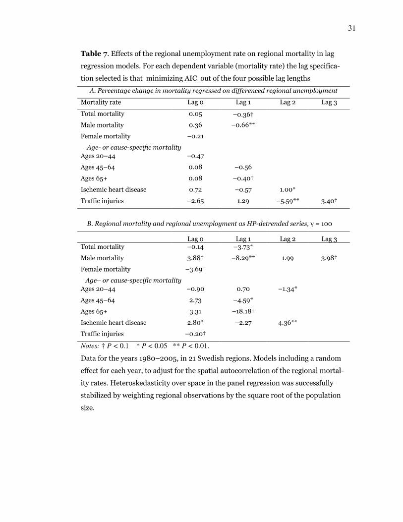
Table 7 Effects of the regional unemployment rate on regional mortality in lag

regression models For each dependent variable (mortality rate) the lag specifica-

tion selected is that minimizing AIC out of the four possible lag lengths

A Percentage change in mortality regressed on differenced regional unemployment

Mortality rate Lag 0 Lag 1 Lag 2 Lag 3

Total mortality 005 ndash036dagger

Male mortality 036 ndash066

Female mortality ndash021

Age- or cause-specific mortality

Ages 20ndash44 ndash047

Ages 45ndash64 008 ndash056

Ages 65+ 008 ndash040dagger

Ischemic heart disease 072 ndash057 100

Traffic injuries ndash265 129 ndash559 340dagger

B Regional mortality and regional unemployment as HP-detrended series γ = 100

Lag 0 Lag 1 Lag 2 Lag 3

Total mortality ndash014 ndash373

Male mortality 388dagger ndash829 199 398dagger

Female mortality ndash369dagger

Agendash or cause-specific mortality

Ages 20ndash44 ndash090 070 ndash134

Ages 45ndash64 273 ndash459

Ages 65+ 331 ndash1818dagger

Ischemic heart disease 280 ndash227 436

Traffic injuries ndash020dagger

Notes dagger P lt 01 P lt 005 P lt 001

Data for the years 1980ndash2005 in 21 Swedish regions Models including a random

effect for each year to adjust for the spatial autocorrelation of the regional mortal-

ity rates Heteroskedasticity over space in the panel regression was successfully

stabilized by weighting regional observations by the square root of the population

size

32 Figure 1 Selected variables used in the study The thin curves are Hodrick-Prescott trends

computed with a smoothing parameter γ = 100

33 Notes Real GDP and average hours indexed to 100 for 2000 and 1992 respectively Mortality is

per 100000 traffic mortality is an age-standardized rate Vertical dotted lines are business-cycle

troughs (OECD chronology)

34

Figure 2 Potential pathways linking economic fluctuations to mortality Black solid arrows

represent positive effects gray dashed arrows negative effects (eg a decrease in economic

activity reduces money income this in turn reduce alcohol consumption which increases

immunity levels) The three rectangles shaded in gray represent final steps directly leading to

an increase in the risk of death Many potential pathways (eg overtime increasing stress and

drinking and decreasing sleep time and social support stress increasing smoking) have been

omitted for clarity

35 Figure 3 Unemployment rate inverted (thick gray line in the four panels) and four age-

or cause-specific mortality rates All series are annual data detrended with the Hodrick-

Prescott filter (γ = 100) and normalized

36

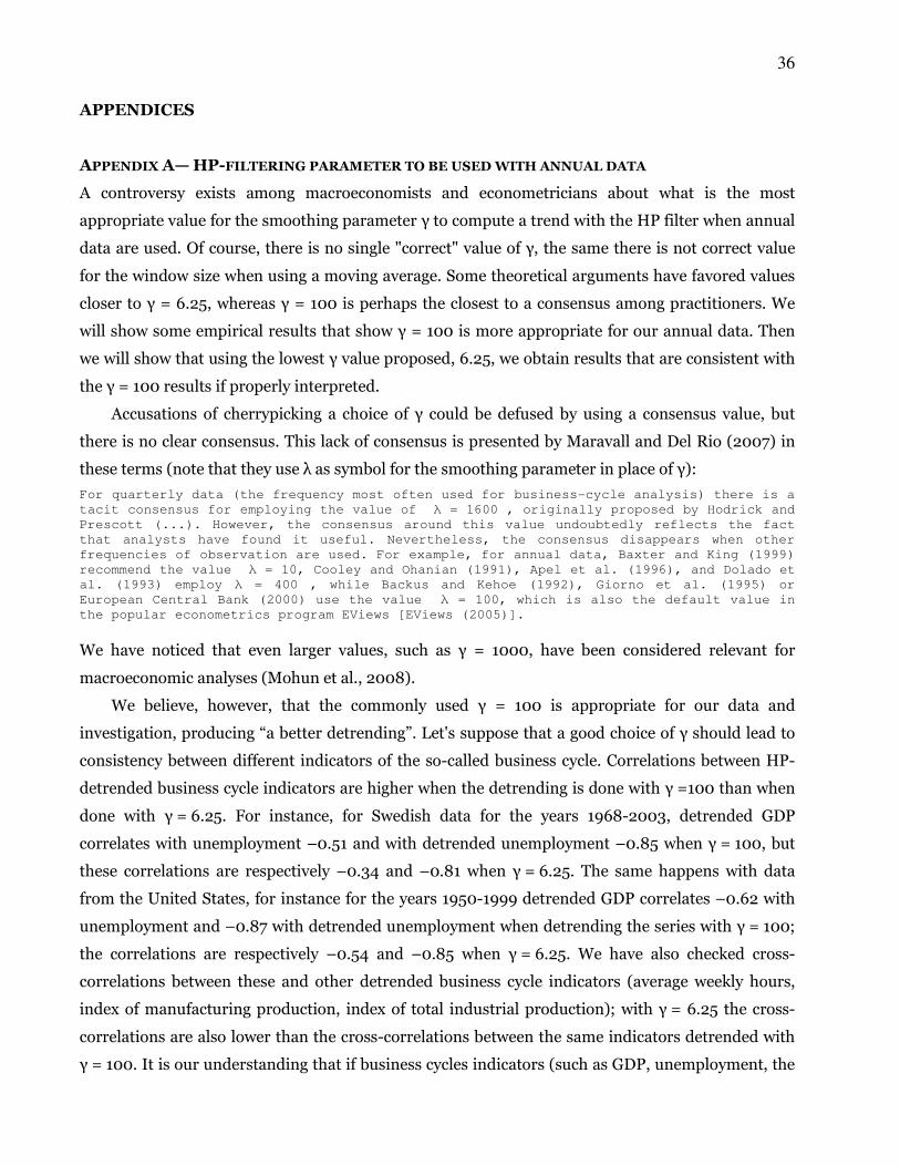
APPENDICES

APPENDIX Amdash HP-FILTERING PARAMETER TO BE USED WITH ANNUAL DATA

A controversy exists among macroeconomists and econometricians about what is the most

appropriate value for the smoothing parameter γ to compute a trend with the HP filter when annual

data are used Of course there is no single correct value of γ the same there is not correct value

for the window size when using a moving average Some theoretical arguments have favored values

closer to γ = 625 whereas γ = 100 is perhaps the closest to a consensus among practitioners We

will show some empirical results that show γ = 100 is more appropriate for our annual data Then

we will show that using the lowest γ value proposed 625 we obtain results that are consistent with

the γ = 100 results if properly interpreted

Accusations of cherrypicking a choice of γ could be defused by using a consensus value but

there is no clear consensus This lack of consensus is presented by Maravall and Del Rio (2007) in

these terms (note that they use λ as symbol for the smoothing parameter in place of γ)

For quarterly data (the frequency most often used for business-cycle analysis) there is a

tacit consensus for employing the value of λ = 1600 originally proposed by Hodrick and

Prescott () However the consensus around this value undoubtedly reflects the fact

that analysts have found it useful Nevertheless the consensus disappears when other

frequencies of observation are used For example for annual data Baxter and King (1999)

recommend the value λ = 10 Cooley and Ohanian (1991) Apel et al (1996) and Dolado et

al (1993) employ λ = 400 while Backus and Kehoe (1992) Giorno et al (1995) or

European Central Bank (2000) use the value λ = 100 which is also the default value in

the popular econometrics program EViews [EViews (2005)]

We have noticed that even larger values such as γ = 1000 have been considered relevant for

macroeconomic analyses (Mohun et al 2008)

We believe however that the commonly used γ = 100 is appropriate for our data and

investigation producing ldquoa better detrendingrdquo Lets suppose that a good choice of γ should lead to

consistency between different indicators of the so-called business cycle Correlations between HP-

detrended business cycle indicators are higher when the detrending is done with γ =100 than when

done with γ = 625 For instance for Swedish data for the years 1968-2003 detrended GDP

correlates with unemployment ndash051 and with detrended unemployment ndash085 when γ = 100 but

these correlations are respectively ndash034 and ndash081 when γ = 625 The same happens with data

from the United States for instance for the years 1950-1999 detrended GDP correlates ndash062 with

unemployment and ndash087 with detrended unemployment when detrending the series with γ = 100

the correlations are respectively ndash054 and ndash085 when γ = 625 We have also checked cross-

correlations between these and other detrended business cycle indicators (average weekly hours

index of manufacturing production index of total industrial production) with γ = 625 the cross-

correlations are also lower than the cross-correlations between the same indicators detrended with

γ = 100 It is our understanding that if business cycles indicators (such as GDP unemployment the

37 index of industrial production etc) are correctly detrended they will measure equally well the

fluctuations of the economy and will correlate at a higher (absolute) value Contrarily if they are

incorrectly detrended their correlation may be weak For instance the correlation between

undetrended GDP and unemployment is almost zero

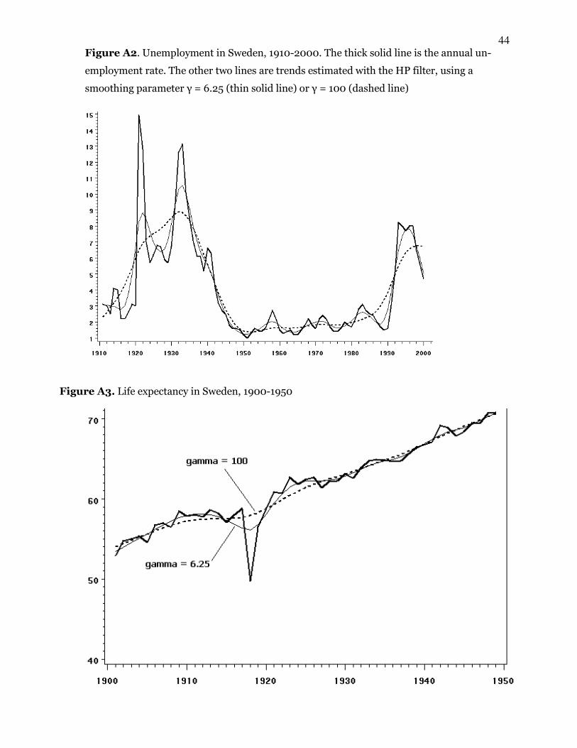
Just by inspection of figure 1 and appendix figure A1 one can argue qualitatively that γ = 100

separates better the trend from the variation around the trend in the annual time series analyzed in

this paper Figure A2 provides extra evidence using Swedish historical data While the trend in the

Swedish unemployment rate computed with γ = 625 oscillates quite wildly in the 1920s-1930s so

that there are two peaks in that trend line corresponding to the unemployment peaks in 1921 and

1933 the trend computed with γ = 100 reveals a single high unemployment period during the 1920-

1930s Another example is shown in figure A3 plotting a time series of annual data for life

expectancy at birth in Sweden for the years 1900ndash1950 In this period demographers agree that the

trend in life expectancy was constantly increasing The original series reveals however a deep trough

in 1918 caused by the world flu pandemics Now that pandemic was only a one-year event and a

procedure that supposedly reveals the trend in the long run should be insensitive to a one-year

deviation That is the case with the HP trend computed with γ = 100 However the trend computed

with γ = 65 is strongly affected by the 1918 drop in life expectancy and shows a declining trend of

life expectancy several years from the mid-1910s to the end of that decade Given that we are

interested in annual variations a detrending method that captures these annual variations (so that

almost none are detected after detrending) does not seem appropriate

Finally tables A1 and A2 show that the results of the paper are not very sensitive to the choice

of γ In both cases statistical significance is slightly higher using γ = 100 rather than γ = 625

Further in table 1 it is necessary to include a lag to GDP and unemployment for γ = 625 in order to

recover the consistency with γ = 100 We believe this is a consequence of the fact that γ = 100 leads

to greater statistical power than γ = 625 This is an important issue overlooked by the theory of

Ravn and Uhlig (2002) which may contribute to explain why practitioners have been slow to adopt

their recommendation of γ = 625 To understand this fact we consider the frequencies removed by

detrending with these different choices of γ

Let us say that γ = 100 removes low frequencies and γ = 625 removes both low and moderate

frequencies In the time domain this means that the trend line for γ = 625 follows the data more

closely (see figure 1 and appendix figures A1 and A2) Examining only high frequencies is a more

rigorous test of a high frequency effect but distributed-lag relationships have their statistical

information spread across all frequencies As long as the desired relationship holds at medium

frequencies one can expect to get greater statistical power by not filtering these frequencies out

Having established that our results are not driven disproportionately by these medium frequencies

it makes the strongest case for our conclusions to include these frequencies in our primary analysis

38 Whereas table A2 shows almost complete consistency between γ = 625 and γ = 100 table A1

has an interesting wrinkle To match the results with γ = 100 it is necessary to include a lag for

unemployment and GDP but not for average hours in manufacturing The explanation for this is

that the distributed lag relationship is primarily at lag one for GDP and unemployment but it is at

lag zero for average hours in manufacturing The simple unlagged correlations in table A1 are

presented as an immediately accessible analysis with neither the complexity nor the additional

modeling assumptions of our subsequent analysis However the consistent lag-zero effect of a lag-

one relationship shows up only in medium to low frequency components which are filtered out by γ

= 625 Thus the analysis restricted to γ = 625 forces us to use the correct lag in table A1 Though

this might be considered desirable it can be considered overall as a disadvantage While the paper

has plenty of technical discussion of lags and tables 5 6 and 7 provide results of lag regression

models table 1 is impressive primarily because of the remarkably consistent pattern of signs across

various measures of health and economic indicators

APPENDIX B mdash ADJUSTMENTS FOR AUTOCORRELATION

The results of lag regression models that are presented in the paper do not present P values adjusted

by using robust standard errors Robust standard errors are known to be substantially more

variable and typically give rise to anti-conservative P values (Kauermann and Carroll 2001) This

mandates using robust standard errors only when there is a clear reason to do so In addition

different robustifications lead to slightly different results requiring robustness analysis on the

specification of the robust standard errors At any rate to show the robustness of our results to the

use of robust standard errors we present some results in table B1 As we anticipated in footnote 7

using robust standard errors the estimated statistical significance is generally slightly higher than

for unmodified standard errors

Table B1 reports Newey-West robust standard errors for the models whose results were

presented in table 5 A robustness analysis showed that these robust standard errors are themselves

robust to the choice of the bandwidth parameter (results not shown) We carried out our robustness

analysis on this table because it concerns the situation where standard Newey-West robust standard

errors are most immediately applicable Table B1 indicates that as proposed in footnote 7 our

unadjusted standard errors are slightly conservative By contrast many investigators have reported

that Newey-West type standard errors are typically anti-conservative (Kauermann and Carroll

2001 and references therein) Thus we view with caution the additional statistical significance

claimed by these methods In situations with positively autocorrelated errors Newey-West type

standard errors may be less over-optimistic than unadjusted errors Here we are however in the

opposite situation with generally negatively autocorrelated errors To convince a skeptic about the

validity of our results the unadjusted standard errors therefore make a stronger argument

39 However presenting adjusted standard errors as additional results makes the argument even

more secure

Table A1 Cross-correlations between three economic indicators life expectancy and selected

mortality rates for Sweden 1968ndash2003

All variables detrended with the

Hodrick-Prescott filter γ = 100

All variables detrended with the

Hodrick-Prescott filter γ = 625

Lag 0 Lag 0 Lag 0 Lag 0 Lag 0 Lag 0 Lag 1 Lag 1

Health indicator Unem-ployment GDP

Avrg hrs in

manuf Unem-ployment GDP

Avrg hrs in

manuf Unem-ployment GDP

Life expectancy 034dagger ndash 015 053 003 011 039 023 ndash023

LE males 038 ndash 019 051 001 014 033dagger 018 ndash016

LE females 028 ndash 010 051 005 007 041 026 ndash026

ASMR all ages ndash 027 021 ndash 040 002 ndash002 ndash032dagger ndash029 032dagger

ASMR males ndash 019 012 ndash 037 005 ndash008 ndash030dagger ndash027 029

ASMR females ndash 031dagger 026 ndash 038 ndash002 004 ndash032dagger ndash030dagger 034dagger

Crude mortality rate

ndash 024 011 ndash 039 005 ndash012 ndash038 ndash027 026

CMR males ndash 017 008 ndash 037 011 ndash017 ndash037 ndash020 020

CMR females ndash 027 014 ndash 038 001 ndash007 ndash036 ndash031dagger 029dagger

Infant mortality ndash 041 024 ndash 016 ndash005 ndash018 ndash007 ndash024 021

0ndash4 ndash 048 036 ndash 034 ndash011 ndash003 ndash016 ndash026 033dagger

5ndash9 ndash 001 ndash 008 ndash 034 010 ndash008 ndash036 005 ndash022

10ndash19 ndash 042 052 ndash 012 ndash012 018 ndash010 000 005

20ndash44 ndash 042 036 ndash 021 ndash005 018 022 019 ndash012

25ndash64 ndash 030dagger 017 ndash 034 ndash019 017 ndash001 ndash005 019

45ndash64 ndash 025 011 ndash 033 ndash019 012 ndash011 ndash018 030dagger

55ndash64 ndash 026 007 ndash 042 ndash020 010 ndash018 ndash017 024

65ndash84 ndash 003 ndash 013 ndash 037 011 ndash018 ndash036 ndash018 030dagger

Notes Correlations with mortality rates are based on n = 36 or close to 36 in most cases in life expectancy

correlations n = 30 ASMR is age-standardized mortality rate

dagger P lt 01 P lt 005 P lt 001 dagger P lt 01

40

Table A2 Effects of the regional unemployment rate on regional mortality in lag

regression models For each dependent variable (mortality rate) the lag specifica-

tion selected is that minimizing AIC out of the four possible lag lengths Series

detrended with the Hodrick-Prescott filter using γ = 625 Compare with table 7 panel

B where γ = 100 was used

Lag 0 Lag 1 Lag 2 Lag 3

Total mortality 095 ndash470

Male mortality 451dagger ndash828

Female mortality ndash166

Age- or cause-specific mortality

Ages 20ndash44 ndash046

Ages 45ndash64 055 ndash398dagger

Ages 65+ 525 ndash2388

Ischemic heart disease 241 ndash293 414

Traffic injuries ndash007

Notes dagger P lt 01 P lt 005 P lt 001

Data for the years 1980ndash2005 in 21 Swedish regions Models include a random

effect for each year to adjust for the spatial autocorrelation of the regional mortal-

ity rates Observations are weighted by the square root of the regional population

to adjust for heteroskedasticity

41 Table B1 Models with a health indicator in first differences regressed on a constant and coincidental and lagged valuesmdashexcept in panel Cmdashof an economic indicator OLS standard errors (SE) below the parameter estimate followed (in square brackets) by Newey-West heteroskedasticity and autocorrela-tion-consistent SE (bandwidth = 2) Marks showing statistical significance next to the parameter estimates correspond to the unadjusted SE (as in table 5) The marks next to the robust SE show the statistical signifi-cance of the corresponding parameter estimates according to the Newey-West methodology Explanatory

variable

Dependent

variable

Lag 0

Lag 1

n

d

R2

Model

Interpretation of the net effect

0027 ndash 0041 31 270a

015 [1] Procyclical mortality

(0019) (0019)

Life expec-

tancy

[0023] [0017]

ndash 0039 0048 32 274 014 [2] Procyclical mortality

(0023) (0023)

Crude mor-

tality

[0031] [0026]dagger

0003 0000 35 246 002 [3]

(0003) (0003)

Mortality

ages 20ndash44

[0003] [0003]

0003 0022dagger 35 176 012 [4] Procyclical mortality

(0012) (0012)

Mortality

ages 45ndash64

[0011] [0007]

ndash 0173dagger 0124 35 289 013 [5] Countercyclical mortality

(0085) (0085)

A

Eco

no

mic

gro

wth

(per

cen

t ra

te o

f

chan

ge

of

real

GD

P)

Mortality

ages 65ndash84

[0130] [0083] [No effect]

ndash 0026 0076dagger 30 264 011 [6] Procyclical mortality

(0042) (0043)

Life expec-

tancy

[0041] [0033]

0076 ndash 0119 34 245 015 [7] Procyclical mortality

(0050) (0050)

Crude mor-

tality

[0043]dagger [0039]

ndash 0006 0002 34 255 002 [8]

(0007) (0007)

Mortality

ages 20ndash44

[0005] [0005]

ndash 0018 ndash 0018 34 162 007 [9]

(0025) (0025)

Mortality

ages 45ndash64

[0016] [0012]

0327dagger ndash 0379dagger 34 245 013 [10] Equivocal Mortality

ages 65ndash84 (0186) (0187)

B

Un

emplo

ym

ent

rate

in

fir

st d

iffe

r-

ence

s

[0136] [0104]

0043dagger 31 296a 011 [11] Procyclical mortality

(0023)

Life expec-

tancy

[0015]

ndash 0059 35 293a 012 [12] Procyclical mortality

(0027)

Crude mor-

tality

[0022]

ndash 0002 33 243 001 [13]

(0004)

Mortality

ages 20ndash44

[0003]

ndash 0033 35 211 014 [14] Procyclical mortality

(0014)

Mortality

ages 45ndash64

[0011]

ndash 0014 35 296a 005 [15]

C

Av

erag

e h

ours

in

man

ufa

cturi

ng

in f

irst

dif

fere

nce

s

Mortality

ages 65ndash84 (0105)

[0079]dagger [Procyclical mortality]

42 dagger P lt 01 P lt 005 a P lt 005 Data include years from 1968 to the early 2000s Estimates statisti-

cally significant at a confidence level of 90 or higher are highlighted in boldface Mortality rates are

measured in deaths per 1000 population life expectancy in years The interpretation of the net effect (last

column to the right) is identical when the standard errors are OLS computed and when they are computed

with the Newey-West method except in two cases in which a new interpretation has been added in

square brackets and italics

43 Figure A1 Selected variables used in the study The thin curves are Hodrick-Prescott trends

computed with a smoothing parameter γ = 625 Compare with figure 1 in which γ = 100

44 Figure A2 Unemployment in Sweden 1910-2000 The thick solid line is the annual un-

employment rate The other two lines are trends estimated with the HP filter using a

smoothing parameter γ = 625 (thin solid line) or γ = 100 (dashed line)

Figure A3 Life expectancy in Sweden 1900-1950

45 REFERENCES

Abdala F Geldstein R N amp Mychaszula S M (2000) Economic restructuring and mor-

tality changes in Argentina ndash Is there any connection In Cornia G A amp Panicciagrave R eds

The mortality crisis in transitional economies (pp 328-350) New York Oxford Univer-

sity Press

Ashley R amp Verbrugge RJ (2006) Coments on A critical investigation on detrending pro-

cedures for non-linear processes Journal of Macroeconomics 28 192-194

Backus D K amp Kehoe O J (1992) International evidence on the historical properties of

business cycles American Economic Review 82 864-888

Baker S OrsquoNeill B amp Karpf R (1984) The injury fact book Lexington MA Lexington

Books

Baxter M amp King RG (1999) Measuring business cycles approximate band-pass filters

for economic time series Review of Economics amp Statistics 81(4) 575-593

Bengtsson T amp Saito O eds (2000) Population amp Economy From Hunger to Modern

Economic Growth Oxford Oxford University Press

Bengtsson T Campbell C Lee J Z et al (2004) Life under PressuremdashMortality and Liv-

ing Standards in Europe and Asia 1700-1900 Cambridge MA The MIT Press

Biddle J E amp Hamermesh D S (1990) Sleep and the allocation of time Journal of Politi-

cal Economy 98 922ndash943

Brenner M H (1971) Economic changes and heart disease mortality American Journal of

Public Health 61(3) 606-611

Brenner M H (1979) Mortality and the national economy A review and the experience of

England and Wales 1936-76 Lancet 2(8142) 568-573

Brenner M H (1982) Economic change and sex-specific cardiovascular mortality in Britain

1955-1976 Social Science amp Medicine 16(4) 431-442

Brenner M H (1987) Relation of economic change to Swedish health and social well-being

1950-1980 Social Science amp Medicine 25(2) 183-195

Brenner M H (1995) Political economy and health In Amick III B C Levine S Tarlov

AR amp Walsh DCeds Society and health New York Oxford University Press

Buchmueller T Grignon M amp Just F (2007) Unemployment and mortality in France

1982ndash2002 CHEPA Working Paper 07-04 Dept of Economics McMaster University To-

ronto

Bunn AR 1979 Ischaemic heart disease mortality and the business cycle in Australia

American Journal of Public Health 69(8) 772-781

Bunn AR 1980 IHD mortality and the business cycle in Australia American Journal of

Public Health 70(4) 409-411

46 Chay K Y amp Greenstone M (2003) The impact of air pollution on infant mortality Evi-

dence from geographic variation in pollution shocks induced by a recession Quarterly

Journal of Economics 118(3) 1121-1167

Chung H 2007 Flexibility for employers or for employees A new approach to examining

labour market flexibility across Europe using company level data In Joslashrgensen H Mad-

sen PK eds Flexicurity and beyond Finding a new agenda for the European social

model (pp 243-277) Copenhagen DJOslashF

Claeskens G amp Hjort N (2008) Model selection and model averaging Cambridge Cam-

bridge University Press

Dagum EB amp Giannerini S (2006) A critical investigation on detrending procedures for

non-linear processes Journal of Macroeconomics 28(1) 175-191

Daly H E (1977) Steady-state economicsmdashThe economics of biophysical equilibrium and

moral growth San Francisco W H Freeman

Dehejia R amp Lleras-Muney A (2004) Booms busts and babiesrsquo health Quarterly Jour-

nal of Economics 119 3 1091-1130

Diggle Peter J (1990) Time seriesmdashA biostatistical introduction Oxford Clarendon Press

Edwards R D (2005) Commentary Work well-being and a new calling for countercyclical

policy International Journal of Epidemiology 34 1222-1225

Edwards R (2008) Who is hurt by procyclical mortality Social Science amp Medicine

67(12) 2051-2058

Eyer J (1976a) Review of Mental-Illness and the Economy International Journal of

Health Services 6(1) 139-148

Eyer J (1976b) Rejoinder International Journal of Health Services 6(1) 157-168

Eyer J (1977) Does unemployment cause a death rate peak in each business cycle Interna-

tional Journal of Health Services 7(4) 625-662

Eyer J (1977b) Prosperity as a cause of death International Journal of Health Services

7(1) 125-150

Eyer J (1984) Capitalism health and illness In McKinlay J B ed Issues in the Political

Economy of Health Care (pp 23-59) New York Tavistock

Fishback P V Haines M R amp Kantor S (2007) Births deaths and New Deal relief dur-

ing the Great Depression Review of Economics amp Statistics 84(1) 1-14

Forbes JB amp McGregor A (1984) Unemployment and mortality in post-war Scotland

Journal of Health Economics 2 239-257

Fridlizius G (1979) Sweden In Lee W R ed European Demography and Economic

Growth London Croom-Helm

Galbraith V L amp Thomas D S (1941) Birth rates and the interwar business cycles Journal

of the American Statistical Association 36(216) 465-475

47 Galloway PR (1988) Basic patterns in annual variations in fertility nuptiality mortality

and prices in pre-industrial Europe Population Studies 42(2) 275-302

Gerdtham U-G amp Johannesson M (2005) Business cycles and mortality Results from

Swedish microdata Social Science amp Medicine 60(1) 205-218

Gerdtham U-G amp Ruhm C (2006) Deaths rise in good economic times Evidence from the

OECD Economics amp Human Biology 4(4) 298-316

Georgescu-Roegen Nicholas (1966) Analytical economics Issues and problems Cam-

bridge Harvard University Press

Georgescu-Roegen N (1971) The entropy law and the economic process Cambridge Har-

vard University Press

Glass GV Willson V L amp Gottman J (1975) Design and analysis of time-series experi-

ments Boulder Colorado Associated University Press

Gonzaacutelez F Quast T (2010) Macroeconomic changes and mortality in Mexico Empirical

Economics March DOI 101007s00181-010-0360-0

Graham JD Chang B amp Evans J (1992) Poorer is riskier Risk Analysis 12 333-337

Gravelle H S Hutchinson G amp Stern J (1981) Mortality and unemployment A critique of

Brenners time-series analysis Lancet 2(8248) 675-679

Higgs R (1979) Cycles and trends of mortality in 18 large American cities 1871-1900 Ex-

plorations in Economic History 16 381-408

Hirsch F (1976) Social limits to growth Cambridge Harvard University Press

Isaacs S amp Schroeder S A (2005) ClassmdashThe ignored determinant of the nations health

New England Journal of Medicine 351(11) 1137-1142

Johansson E (2004) A note on the impact of hours worked on mortality in the OECD Eu-

ropean Journal of Health Economics 4 335-340

Junankar PN (1991) Unemployment and mortality in England and Wales a preliminary

analysis Oxford Economic Papers 43 305-320

Kasl S (1979) Mortality and the business cycle some questions about research strategies

when utilizing macro-social and ecological data American Journal of Public Health

69(8) 784-789

Kauermann G Carroll RJ (2001) A note on the efficiency of sandwich covariance JASA

961387-1496 (httpwwwjstororgstable3085907)

Khang YH Lynch J amp Kaplan-Oso G (2005) Impact of economic crisis on mortality in

South Korea International Journal of Epidemiology 34(6) 1291-1301

Laporte A (2004) Do economic cycles have a permanent effect on population health Re-

vising the Brenner hypothesis Health Economics 13 767-779

Layne L J (2007) Appendix 4 Spatial autocorrelation In Stephen J Kunitz The Health of

Populations New York Oxford University Press

48 Lee R (1981) Short-term variationmdashVital rates prices and weather In Wrigley E A amp

Schofield R S The population history of England 1541-1971--A reconstruction (pp 356-

401) London Edward Arnold

Lew A (1979) Mortality and the business cycle how far can we push an association

American Journal of Public Health 69 782-783

Liu Y Tanaka H amp Fukuoka Heart Study Group (2002) Overtime work insufficient sleep

and risk of non-fatal acute myocardial infarction in Japanese men Occupational amp Envi-

ronmental Medicine 597 447-451

Livi-Bacci M (1991) Population and nutritionmdashAn essay on European demographic his-

toryNew York Cambridge University Press

Maravall A amp del Riacuteo A (2007) Temporal aggregation systematic sampling and the

HodrickndashPrescott filter Computational Statistics amp Data Analysis 52(2)975-998

McAvinchey ID (1984) Economic factors and mortality some aspects of the Scottish case

1950-1978 Scottish Journal of Political Economy 31(1) 1-27

McKee Martin amp M Suhrcke (2005) Commentary Health and economic transition Inter-

national Journal of Epidemiology 34 1203-1206

McKinlay J B McKinlay S M amp Beaglehole R (1989) Trends in death and disease and

the contribution of medical measures In Freeman H E amp Levine S eds Handbook of

medical sociology 2nd ed (pp 14-45) Englewood Cliffs NJ Prentice Hall

Mishan E J (1970) Technology and growthmdashThe price we pay New York Praeger

Mitchell W C (1951) What happens during business cyclesmdashA progress report New York

National Bureau of Economic Research

Mohun S amp Veneziani R (2008) Goodwin cycles and the US economy 1948-2004 In

Flaschel P Landesmann M eds Mathematical economics and the dynamics of capital-

ism Godwins legacy continued (pp 107-130) New York Routledge

Neumayer E (2004) Recessions lower (some) mortality ratesmdashEvidence from Germany

Social Science amp Medicine 58(6) 1037-1047 [corrigendum in Social Science amp Medicine

59(9]

OECD OECD Composite Leading Indicators Reference Turning Points Accessed in 2006 in

httpwwwoecd orgdocument4102340en_2649_34349_1891177_1_1_1_100html

Ogburn W F (1964) The fluctuations of business as social forces [1923] In Duncan O D

ed William F Ogburn on culture and social change (pp 235-246) Chicago University of

Chicago Press

Ogburn W F amp Thomas D S (1922) The influence of the business cycle on certain social

conditions Journal of the American Statistical Association 18 324-340

49 Organisation for Economic Co-operation and Development 2006

httpwwwoecdorgdocument4102340en_2825_495677_1891177_1_1_1_100html

(consulted in September 2006)

Randolph Beard T amp Lozada G (1999) Economics entropy and the environmentmdashThe

extraordinary economics of Nicholas Georgesccedilu-Roegen Northampton MA Edward El-

gar

Ravn MO amp Uhlig H (2002) On adjusting the Hodrick-Prescott filter for the frequency of

observations Review of Economics amp Statistics 84(2) 371-380

Ruhm CJ (2000) Are recessions good for your health Quarterly Journal of Economics

115(2) 617-650

Ruhm C J (2004) Macroeconomic conditions health and mortality Cambridge MA Na-

tional Bureau of Economic Research NBER Working Paper 11007

Ruhm C J (2005a) Commentary Mortality increases during economic upturns Interna-

tional Journal of Epidemiology 34 1206-1211

Ruhm C J (2005b) Macroeconomic conditions and deaths from coronary heart disease

NBER and University of North Carolina Greensboro NC

Ruhm C J (2005c) Healthy living in hard times Journal of Health Economics 24 341ndash

363

Ruhm C J (2006) Macroeconomic conditions health and mortality In Jones A M ed

The Elgar companion to health economics Cheltenham UK Edward Elgar

Ruhm C J (2008) Macroeconomic conditions health and government policy In Schoeni

R F House J S Kaplan G amp Pollack H Making Americans healthier Social and eco-

nomic policy as health policy New York Russell Sage

Schofield R (1985) The impact of scarcity and plenty on population change in England

1541-1871 in Rotberg R I et al eds Hunger and history The impact of changing food

production and consumption patterns on society New York Cambridge University Press

Shryock HS Siegel J S et al (1973) The methods and materials of demography Wash-

ington DC US Bureau of the Census

Soslashgaard J (1992) Econometric critique of the economic change model of mortality Social

Science amp Medicine 34(9) 947-957

Sokejima S amp Kagamimori S (1998) Working hours as a risk factor for acute myocardial

infarction in Japan a case-control study BMJ 317 775ndash80

Statistics Sweden (2005) wwwscbse Data downloaded in 2005-2009

Svensson M (2007) Do not go breaking your heart Do economic upturns really increase

heart attack mortality Social Science amp Medicine 65 833-841

Svensson M (2010) Economic upturns are good for your health but watch out for acci-

dents a study on Swedish regional data 1976ndash2005 Applied Economics 42(5)615 - 625

50 Tapia Granados JA (2005a) Recessions and mortality in Spain 1980-1997 European

Journal of Population 21(4) 393-422

Tapia Granados JA (2005b) Increasing mortality during the expansions of the US econ-

omy 1900-1996 International Journal of Epidemiology 34(6) 1194-1202

Tapia Granados JA (2005c) Economic growth business fluctuations and health progress

International Journal of Epidemiology 34(6) 1226-1233

Tapia Granados JA (2006) Mortality effects of the economic crisis in South Korea Inter-

national Journal of Epidemiology 35(5)1357

Tapia Granados JA (2008) Economic fluctuations and mortality in postwar Japan De-

mography 45(2) 323-343

Tapia Granados J A amp E L Ionides (2008) The reversal of the relation between economic

growth and health progress Sweden in the 19th and 20th centuries Journal of Health Eco-

nomics 27544ndash563

Tapia Granados J A amp Diez Roux AV (2009) Life and death during the Great Depression

Proceedings of the National Academy of Sciences of the USA 106(41)17290ndash17295

Tapinos G P Mason A amp Bravo J (1997) Demographic responses to economic adjust-

ment in Latin America New York Clarendon Press

Thomas D S (1927) Social aspects of the business cycle New York Knopf

Thomas D S (1941) Social and economic aspects of Swedish population movements

1750-1933 Macmillan New York

Valkonen T Martikainen P et al (2000) Changes in socioeconomic inequalities in mortal-

ity during an economic boom and recession among middle-aged men and women in

Finland European Journal of Public Health 10(4)274-280

Venables WN amp Ripley D D (2002) Modern applied statistics with S 4th ed New York

Springer

Wagstaff A (1985) Time series analysis of the relationship between unemployment and

mortality A survey of econometric critiques and replications of Brenners studies Social

Science amp Medicine 21(9) 985-996

Winter J (1983) Unemployment nutrition and infant mortality in Britain 1920-50 in The

Working Class in Modern British History Essays in Honour of Henry Pelling Cambridge

University Press Cambridge

WHO-HFA (2005) Heath For All Database European Regional Office World Health Or-

ganization httpwwweurowhointhfadb Data downloaded between 2005 and 2010

Zolotas X (1981) Economic growth and declining social welfare AthensNew York Bank

of GreeceNew York University Press

2 rates and business-cycle indicators These results adds to an emerging consensus that eco-

nomic expansions rather than recessions have harmful effects for health

The next two sections review previous work on mortality and the business cycle and po-

tential pathways linking the economy with mortality Sections 4 and 5 show the data and

methods we have used for the investigation and the results of our analyses The last two sec-

tions include a discussion of the results of other investigations and a general discussion of

our findings in the context of previous work In two appendices we have discussed statistical

issues that are probably beyond the interest of the average reader of this paper

2 Previous Research on Mortality and the Business Cycle

The relation between mortality and the business cycle was already investigated in the 1920s

by Ogburn and Thomas who were surprised by finding a procyclical fluctuation of mortality

in the United States and Britain during the business cycles preceding World War I (Ogburn

1964 Ogburn and Thomas 1922 Thomas 1927) These early studies were largely forgotten

for most of the 20th century probably because the idea that mortality evolves better during

recessions than during expansions was too counterintuitive to be easily accepted

The notion that economic hardship must be bad for health and therefore associated with

higher mortality is deeply ingrained in social science Many investigations in the fields of

public health demography and economics have shown that low income is systematically

associated with higher death rates (Isaacs and Schroeder 2005) Increasing mortality result-

ing from a worsening standard of living is the basis of Malthusrsquos ldquopositive checkrdquo to popula-

tion growth which is a frequent working hypothesis in demography and economic history

(Bengtsson and Saito 2000 Bengtsson et al 2004) Historical studies of preindustrial socie-

ties have indeed shown that mortality upswings are associated for instance with bad har-

vests increases in grain prices or cold winters (Lee 1981 Schofield 1985 Thomas 1941 Livi-

Bacci 1991) However this link between mortality and food price inflation or bad harvests is

considerably weakened with advances in economic development and industrialization (Gal-

loway 1988) In Sweden for example the strong mortality responses to bad harvests ob-

3 served in the 18th century and first half of the 19th century (Fridlizius 1979) disappeared

during the last decades of the 19th century (Thomas 1941 Tapia Granados and Ionides

2008)

In the 1970s and 1980s Brenner repeatedly reported harmful effects of recessions on

mortality other health indicators and social conditions (Brenner 1971 1979 1982 1987)

Brenner utilized relatively unconventional econometric techniques such as Fourier analysis

distributed lag regressions and ARIMA models These studies mostly published in health

journals raised protracted controversy While the results of a few investigations apparently

supported Brenners argument to some extent (Bunn 1979 1980 Junankar 1991 McAv-

inchey 1984) other researchers criticized Brennerrsquos studies for deficient presentation of data

and methods use of lags arbitrarily chosen lack of statistical power with the number of ob-

servations being often close to that of covariates improper methods of detrending and in-

clusion of multiple covariates implying strong collinearity (Eyer 1976a 1976b 1977a Kasl

1979 Gravelle Hutchinson and Stern 1981 Forbes and McGregor 1984 Lew 1979 Winter

1983 Soslashgaard 1992 Wagstaff 1985) Meanwhile with straightforward statistical methods

Eyer (1977b) Higgs (1979) and Graham et al (1992) again found a procyclical fluctuation of

mortality in the United States

In recent years a number of publications have reexamined whether macroeconomic fluc-

tuations are related to short-term oscillations in mortality In a ground-breaking study

Ruhm (2000) applied panel regressions to data from the 50 states of the United States dur-

ing the years 1972ndash1991 showing that beyond long-term trends periods of expanding eco-

nomic activitymdashgauged by low state unemployment levelsmdashwere associated with increased

mortality that is to say that mortality oscillates procyclically Other work using panel re-

gressions has shown that the 1981ndash1982 recession induced substantial reductions of atmos-

pheric pollution associated with significant drops in infant mortality (Chay and Greenstone

2003) that babies born during recessions in the United States have a reduced incidence of

low birth weight and lower infant mortality (Dehejia and Lleras-Muney 2004) and that

death rates oscillate procyclically in Japan (Tapia Granados 2008) the 16 German states

4 (Neumayer 2004) the 50 Spanish provinces (Tapia Granados 2005a) the 96 French deacute-

partements (Buchmueller at al 2007) and the 23 OECD countries (Johansson 2004 Gerd-

tham and Ruhm 2006) The procyclical oscillations of mortality in the United States have

also been confirmed using time-series analyses (Laporte 2004 Tapia Granados 2005b) and

individual-level data from the National Longitudinal Mortality Study (Edwards 2008) The

evolution of mortality rates and life expectancy in the United States during the 1920s and

1930s shows that mortality-based health indicators evolved better during the Great Depres-

sion of 1929-1933 than during the economic expansions of the ldquoroaringrdquo twenties and mid-

thirties (Tapia Granados and Diez Roux 2009) In medium-income market economies mor-

tality responses to macroeconomic downturns have been found to be erratic (Tapinos et al

1997) or even clearly procyclical (Abdala et al 2000 Khang et al 2005 Tapia Granados

2006 Gonzaacutelez and Quast 2010)

Sweden has been the focus of four recent studies by Gerdtham and Johannesson (2005)

Tapia Granados and Ionides (2008) and Svensson (2007 2010) which provide conflicting

evidence on the relation between macroeconomic fluctuations and mortality in that country

The existence and nature of this relation in Sweden seems important because (a) Sweden is a

world leader in health indicators and levels of income per capita (b) the Swedish welfare

state is one of the most developed in the world with universal health care and generous in-

come support for unemployed people provided by the State and (c) the Swedish economy

went through major fluctuations in the last decades of the 20th century (see for instance the

wide fluctuations of unemployment figure 1)

The study by Gerdtham and Johannesson (2005) used a sample of 47484 adults inter-

viewed in Sweden in 1980ndash1996 and followed through the end of 1996 for a total of 6571

deaths Using a probit model Gerdtham and Johannesson modeled the probability of death

as a function of age the state of the economy (proxied by a business-cycle indicator) and a

linear trend They found mortality increasing during economic downturns and decreasing in

upturnsmdashie a countercyclical fluctuation of mortalitymdashthough only for male mortality and

only for four business-cycle indicators (notification rate capacity utilization confidence in-

5 dicator and GDP growth) out of six that they considered (the aforementioned plus unem-

ployment and GDP deviation from trend)

Tapia Granados and Ionides (2008) investigated the relation between economic growth

and health progress in Sweden during the 19th and 20th centuries They found that annual

economic growth was positively associated with mortality decline throughout the 19th cen-

tury though the relation became weaker as time passed and was reversed in the second half

of the 20th century during which higher economic growth was associated with lower drops

in mortality While the economy-related effect on health occurs mostly at lag zero in the 19th

century the effect is lagged up to two years in the 20th century These results implying a pro-

cyclical fluctuation of mortality rates after 1950 were found to be robust across a variety of

mortality rates (sex- age- and age- and-sex-specific) statistical procedures (including linear

regression spectral analysis and lag regression models) and economic indicators (GDP per

capita growth unemployment and some measures of inflation) This study did not investi-

gate effects for periods shorter than a half century or for cause-specific mortality but its re-

sults indicate that macroeconomic changes (indexed by annual GDP growth or the annual

change in unemployment) have a lagged effect on the annual change in mortality mostly at

lag one

In two different studies Svensson (2007 2010) has employed panel regressions to analyze

annual rates of mortality and unemployment in the 21 Swedish regions during 1976ndash2005

He could not detect any relation between mortality (neither total nor sex-specific) and un-

employment that was robust to different specifications including year-fixed effects region-

specific linear trends or other methods to avoid potential bias Therefore he was unable to

replicate the countercyclical oscillation of male mortality reported by Gerdtham and Johan-

nesson (though Svensson downplays this inconsistency between his results and those of

Gerdtham and Johannesson) The only robust procyclical oscillation found by Svensson is

for mortality due to work-related injuries which increase in expansions Other cause-

specific mortality rates were found to be procyclical or countercyclical depending on the

specification Svensson found ischemic heart disease mortality to be consistently counter-

6 cyclical though only among those aged 20 to 49 and at the 01 level of statistical signifi-

cance

3 Pathways Linking the Economy and Mortality

Potential pathways leading to a procyclical fluctuation of mortality (figure 2) have been ex-

tensively discussed elsewhere (Ruhm 2000 2004 2005a Tapia Granados 2005a Eyer

1984 Neumayer 2004) They will only be briefly summarized here

Mortality caused by diseases of the circulatory system that is cardiovascular disease

(CVD) mortality is usually the main component of total mortality in most countries It has

been hypothesized that procyclical oscillations of CVD mortality may result from a variety of

CVD risk factors that increase during expansions (Eyer 1977b Ruhm 2000 2005b Tapia

Granados 2005b 2008) These would include stress in the working environmentmdashbecause

of overtime and increased rhythm of work (Sokejima and Kagamimori 1998)mdash reduced

sleep time (Biddle and Hamermesh 1990) atmospheric pollution smoking and consump-

tion of saturated fat and alcohol (Ruhm 2005c) Many of these factors might increase the

risk of death of persons who had a previously developed chronic disease such as cancer

diabetes a respiratory illness or a chronic infection The increase in traffic deaths during

economic booms and the decrease in recessions is a robust finding across countries (Eyer

1977b Ruhm 2000 Neumayer 2004 Tapia Granados 2005a 2005b Khang et al 2005)

The strong procyclical fluctuation of traffic-related injuries and deaths is intuitively ex-

plained by the fact that commuting commercial and recreational traffic rapidly expand in

economic upswings (Baker et al 1984 Ruhm 2000) and the effect is probably aggravated by

the procyclical change in alcohol consumption and by sleep deprivation in expansionary pe-

riods in which overwork is frequent (Biddle and Hamermesh 1990 Liu et al 2002)

Increased infant mortality in expansions has been related to economic activity through

atmospheric pollution (Chay and Greenstone 2003) and healthier behaviors of pregnant

women during recessions (Dehejia and Lleras-Muney 2004) In addition in high-income

economies injury deaths are a quite large proportion of the small annual number of infant

7 and children deaths Thus in this context economic expansions could be associated to an

above-trend level of infant and child mortality through car crashes as well as domestic or

school injuries related to overworked parents or caretakers

4 Data and Methods

In the present investigation crude and sex- and age-specific mortality rates were computed

from deaths and population in five-year age strata taken from Statistics Sweden (2005)

Data on annual unemployment rates real GDP industrial production and the confidence

indicator for the manufacturing industry were obtained from the same source Infant mor-

tality and age-standardized mortality rates were taken from the WHO-HFA (2005) data-

base4 Four indices of Swedish manufacturing activity (average hours aggregate hours

manufacturing output and manufacturing employment) were obtained from the US Bureau

of Labor Statistics (2005) Data on life expectancy at birth are from the Human Mortality

Database (2005)

Our main analysis employs data from Swedish annual statistics (figure 1) from 1968 to

the early 2000s (usually until 2003 with n equal to 35 or 36 in most series) This time frame

was chosen for two reasons first because it is possible that the relation between macroeco-

nomic changes and health progress changed over time and the focus of this investigation is

contemporary Sweden second because a number of cause-specific and agendashadjusted mor-

tality rates for Sweden are available from the WHO Health-For-All database beginning in

1968 or 1970 The reference chronology of the Organisation for Economic Cooperation and

Development (OECD 2006) indicates that there were 10 business cycle troughs in Sweden

(figure 1) between 1968 and 2003

4 In the HFA database age-standardized rates are computed with the direct method applying age-

specific rates for 5-year age-strata (0-4 5-9 etc) to a standard European population For instance

the standardized rate of cancer mortality at ages 0-64 represents what the age-specific rate at ages 0-

64 would have been if the Swedish population aged 0-64 had the same age distribution as the stan-

dard European population

8 Population health is indexed by life expectancy at birth (e0 ldquolife expectancyrdquo for brevity)

and a variety of age- sex- and cause-specific mortality rates Since life expectancy is the best

mortality-based summary index of population health unaffected by the age structure of the

population and allowing intertemporal and cross-sectional comparisons (Shryrock et al

1973) we based many of our analysis in ∆e0 the annual gain in life expectancy as a major

indicator of health progress

Analyses in this paper are either (a) simple correlation models between health and eco-

nomic indicators or (b) lag regressions in which a health indicator is regressed on contem-

poraneous and lagged values of an economic indicator Strong collinearity between business

cycle indicators precludes using combinations of these indicators in the same multivariate

regression model Since both the indicators of population health and the economic indica-

tors used in the study have obvious trends (figure 1) all variables were detrended before

analysis to produce trend-stationary series Several procedures to detrend variables were

used only results obtained either with ldquoHP detrendedrdquo series (ie series obtained by sub-

tracting the trend computed with the Hodrick-Prescott filter5 from the actual value of the

variable) or with variables transformed into first differences (∆xt = xt ndash xt-1) or rate of change

(∆xtxt-1) are presented Other detrending procedures6 were employed in sensitivity analyses

and yielded similar results

Macroeconomic fluctuations are not easy to identify and delimit and not all the different

business cycle indicators gauge them in the same way (Mitchell 1951 Backus et al 1992

Baxter and King 1999) In the present study eight economic indicators were used GDP the

unemployment rate the index of industrial production the confidence indicator and four

indices of activity in manufacturing average working hours aggregate hours output and

employment All of them show significantly correlated fluctuations except the confidence

indicator which fluctuates without a definite relation to the others For the sake of brevity

5 We used a smoothing parameter γ = 100 (figure 1) as advised for annual data (Backus and Kehoe

1992) Appendix A defends this option

6 We used the HP filter applied with γ = 10 and the band-pass filter BP(28) recommended by Baxter and King (1999)

9 results for only three business cycle indicatorsmdashreal GDP the unemployment rate and the

index of average working hours in manufacturingmdashwill be presented here At lag zero de-

trended unemployment and GDP have a strong negative correlation in this Swedish sample

(ndash 075 when both series are in rate of change ndash 085 when both are detrended with the

Hodrick-Prescott filter for both correlations P lt 0001) The index of average hours worked

in manufacturing correlates positively and significantly with unemployment (040 P = 001

both series HP-detrended) at lag zero Therefore both unemployment and average hours are

countercyclical while GDP is procyclical7

Cross-correlations and distributed lag regression models were used to ascertain the con-

comitant variation between ldquohealthrdquo and ldquothe economyrdquo or the coincident or lagged effect of

the latter on the former Cross-correlations between detrended series have been used to ana-

lyze the historical properties of business cycle indicators (Galbraith and Thomas 1941

Backus and Kehoe 1992) biological and medical data (Diggle 1990) and time-series ex-

periments (Glass et al 1975) Distributed lag regressions are a common tool in econometrics

For the sake of consistency the two variables correlated or used as outcome and explanatory

variables in a regression were always detrended by the same method8 In lag regressions we

used the Akaike information criterions (AIC) as an objective approach to choose among the

multiple models that we investigated Although AIC has its strengths and flaws relative to

other model selection criteria such as BIC and adjusted R2 (Claeskens 2008) to minimize

AIC is a common and generally accepted procedure to choose ldquothe bestrdquo model among mod-

els with different lags

7 Business cycle data for the United States and other industrialized countries show average working

hours in manufacturing as a procyclical indicator in Sweden however its strong positive correlation

with unemployment shows that it is clearly a countercyclical one We comment on the potential

causes of this difference in the general discussion section

8 In fact there is an exception to this rule because in some models first differences in e0 or mortality

are regressed on the rate of growth of GDP GDP growth is a major dynamic index of business condi-

tions and moreover because of the exponential growth of real GDP first differences tend to present

exploding heteroskedasticity when the series exceeds a few observations

10 In supplementary analyses utilizing panel regression models we also analyzed Swed-

ish mortality rates and unemployment rates for the 21 Swedish regions in the years 1976ndash

2005 These data were kindly shared with us by Mikael Svensson and correspond to the

data used in his two papers (Svensson 2007 and 2010) We obtained the population data for

the regional analysis from Statistics Sweden

5 Results

51 Correlation Models

For the whole population and for large age groups and with series HP-detrended mortality

has positive correlations with GDP and negative correlations with unemployment and aver-

age hours (table 1) Life expectancy at birth e0 follows the same pattern with reversed signs

as is to be expected if mortality is procyclical9 Out of 54 correlations of detrended economic

indicators with detrended health indicators (table 1) only four correlations have a sign that

is inconsistent with a procyclical oscillation of mortality

When age- and sex-specific mortality rates are correlated with the economic indicators

with variables either HP-detrended (table 2 bottom panel) or in rate of change (table 2 top

panel) the correlations of the HP-detrended variables with the economic indicators are

much stronger However the direction of the correlations is consistently similar in analyses

involving rate of change or HP-detrended series suggesting that the HP-filtering is not in-

troducing spurious results in terms of the sign or direction of correlations with mortality

rates Leaving aside the correlations that are statistically indistinguishable from zero almost

without exception the correlations of age- and sex-specific mortality rates with unemploy-

ment and average hours are negative while the correlations of mortality rates with GDP are

positive (table 2) As observed for larger demographic groups (table 1) the pattern of signs

in the correlations of age-and sex-specific mortality rates (table 2) indicate a procyclical os-

9 The other three manufacturing indicators (aggregate hours output and employment) and the index

of industrial production correlate similarly with mortality and e0 The confidence indicator has erratic

correlations with both the other business cycle indicators and with the health indicators

11 cillation of mortality for most age groups The high correlations between detrended busi-

ness cycle indicators and detrended mortality for ages 10ndash19 and 20ndash44 are apparent in the

fluctuations of these death rates following the swings of the economy (figure 3)

During the period of the study the unemployment rate oscillated very moderately in

Sweden before 1990 never exceeding 3 but in the early 1990s unemployment rose to

around 10 remaining there for most of the decade (figure 1) Correlations between mortal-

ity rates and economic indicators computed in split samples corresponding to the years in

which unemployment was low (1968ndash1989) or high (1989ndash2003) reveal that the results are

quite robust (table 3) In split samples the correlations of life expectancy and mortality rates

with the countercyclical unemployment and average hours and with the procyclical GDP all

show an increase in death rates during expansions However with smaller samples fewer

results are significant and in some cases even coefficient signs are unstable

The zero-lag correlations of detrended series of cause-specific mortality with detrended

economic indicators (table 4) indicate a strong procyclical oscillation of traffic mortality

which shows strong positive correlations with GDP and strong negative correlations with

unemployment and average hours CVD mortality does not reveal any clear relation with

business fluctuations at lag zero One of its components ischemic heart disease mortality or

ldquoheart attacksrdquomdashcausing about one half of total CVD deathsmdash correlates negatively with GDP

(ndash 029) and positively (028) with unemployment at marginal or not significant levels

when considering all ages However at ages over 64 the correlations have the same sign but

they are much stronger all of which suggests that ischemic heart disease at advanced ages

fluctuates countercyclically in Sweden when considering lag zero effects only Cerebrovas-

cular disease (stroke) mortality comprises about one fifth of all CVD deaths and does not re-

veal any definite relation with business cycle indicators at lag zero10

10 Table 4 and other tables omit the results for cancer respiratory disease infectious disease flu

suicide and homicide causes for which we could not find a conclusive relation with macro-economic

fluctuations

12 52 Lag Regression Models

We explored the joint effect on health of coincidental and lagged changes in the economy

with models of the type sum = minus+=p

i itit xH0βα including p lags in which Ht is a health indica-

tor at year t and xtndashi is an economic indicator at year t ndash i In these models health is indexed

by e0 or an age-specific mortality rate and the explanatory variable is either unemployment

GDP or average hours in manufacturing Variables are detrended by conversion either in

first differences or in rate of change In general in models using different methods of de-

trending the estimated effects were consistent in sign For a variety of health indicators we

explored models in which the economy is indexed by an indicator (GDP unemployment or

average hours) including several lags (table 5) For life expectancy crude mortality or age-

specific mortality for large age-groups (table 5) AIC values indicate that models including a

coincidental effect at lag zero and a lagged effect at lag one are to be preferred when the eco-

nomic indicator used as regressor is GDP growth or the change in unemployment However

when the regressor is average hours the models including lag zero only are those that mini-

mize AIC All these distributed lag models in which either GDP or unemployment is the eco-

nomic covariate (table 5 panels A and B) show a significant effect on health at lag one but

when the economic indicator is average hours the effect is at lag zero GDP growth has a sig-

nificant negative effect on life expectancy while unemployment and average hours have sig-

nificant positive effects Similar patterns are observed for crude mortality or mortality for

specific ages Interpreting the sign of the net effect most of these models suggest procyclical

mortality but considering the size of the net effect (adding up effects at lags zero and one)

only the model for mortality at ages 45-64 regressed on GDP growth (table 5 panel A)

reaches marginal significance (the net effect is 0003 + 0022 = 0025 has an standard error

SE = 0013 P = 009) Models with average hours as economic indicator (table 5 panel C)

only require one lag and they suggest procyclical mortality when the economic indicator is

either life expectancy crude mortality or mortality at ages 45-64

13 In these regression models (table 5) the Durbin-Watson d is usually either close to 20

or above 20 Since d = 2 [1 ndash r] where r is the estimated autocorrelation d gt 2 implies evi-

dence against positive autocorrelation of the residuals which would result in underestimates

of standard errors and spurious significance 11

We also examined some models in which an age-standardized mortality rate is regressed

on coincidental or lagged GDP growth (table 6) For all-cause mortality sex-specific age-

adjusted mortality for both males and females and sex-specific age-adjusted mortality in

ages 25ndash64 (table 6 panel A) the specification minimizing AIC is the one including effects

at lags zero and one With only a few exceptions in which lag-two effects are also needed this

is also true for CVD mortality in different demographic groups (table 6 panel B) However

for traffic mortality (table 6 panel B bottom) the minimization of AIC occurs in specifica-

tions including just lag-zero effects

For total mortality male mortality and female mortality and for male mortality at ages

25-64 predominantly positive and statistically significant effects of GDP growth on mortality

at lag one indicate a procyclical oscillation of mortality rates For CVD mortality at all ages

and ages below 65 positive (and significant) effects of GDP growth at lag one also indicate a

procyclical oscillation of this type of mortality However for CVD mortality at ages 65 and

over what predominates is negative effects of GDP growth (at lags zero and two)

In regressions modeling coincidental and lagged effects of GDP growth on ischemic heart

disease mortality (table 6 panel B) almost without exception there are negative effects at lag

zero and positive effects at lag one and the positive effects at lag one are often statistically

significant and predominant However for ischemic heart disease mortality in males the

11 In only a few cases d is large enough to suggest negative autocorrelation (see footnote in table 5)

Adjusting for autocorrelation of the residuals did as expected produce similar parameter estimates

with some additional statistical significance To avoid the need to justify selection of a specific autocor-

related model we simply present the conservative unadjusted values For further discussion of these

issues see appendix B

14 model minimizing AIC also includes effects at lag two and the net effect of GDP growth on

this type of mortality in males is negative ie ischemic heart disease mortality decreases

with greater GDP growth Overall this indicates a countercyclical oscillation of ischemic

heart disease mortality However the effects at lag two are difficult to interpret Business

cycles over recent decades in Sweden last approximately 4 years (according to the OECD

chronology the mean + SD of the trough-to-trough distance is 38 + 14 years) This implies

that an effect of high GDP growth lagged two years will likely occur actually when GDP

growth is already low in the next phase of the cycle For ischemic heart disease at ages 85

and over there are negative effects at lags zero and two and a significant positive effect at lag

one so that the net effect of GDP growth is negative the positive effect for lag one is statisti-

cally significant but the net effect is not

Overall considering lag regression models (tables 5 and 6) and correlations (tables 1 to 4)

for the period 1968-2003 the results are consistent for major health indicators Results for

life expectancy total mortality and crude or age-adjusted total mortality in large age groups

indicate a procyclical fluctuation of death rates for the whole population and for both males

and females Less consistent are the correlations and regression results for age-specific mor-

tality rates The link between economic expansions (recessions) and increases (falls) in mor-

tality rates seems to be stronger in adolescents young adults and adults of middle age In-

fant mortality also fluctuates procyclically Results for ages 65-84 or over 65 are equivocal

and for mortality at ages 85 and over we could not find any statistically significant evidence

of a link with business cycle fluctuations

53 Size of the Effect

The net effects of GDP growth at lags zero) and lag one (ndash 097 +335 = 232) on total age-

adjusted mortality measured per 100000 population (table 6 panel A) imply that each extra

percentage point in GDP growth will increase mortality in about 232 deaths per 100000 In

recent years the age-standardized death rate is 600 per 100000 Since the Swedish popula-

tion is about 9 million each percentage point increase in GDP growth would cause

15 [232105] middot 9 106 = 209 extra deaths or an increase of a slightly less than half a percent

(232600 = 04) in age-adjusted mortality During the period of study GDP growth oscil-

lated between ndash2 in major downturns and 6 in major expansions Therefore a typical

expansion in which GDP growth increases three or four percentage points would increase

age-adjusted mortality between one and two percentage points with an additional death toll

of 600 to 800 fatalities

Modeling the relation between macroeconomic change and health using the annual varia-

tions in unemployment (∆Ut ) and life expectancy (∆e0 t) the estimated equation (error term

omitted) is

∆e0t = 0164 ndash 0026 middot ∆Ut + 0076 middot ∆Ut -1 (this is model [6] in table 5) It implies a gain of 0164 years in life expectancy from time t-1

to time t after no change in unemployment from time t-2 to time t-1 and from time t-1 to

time t (that it ∆Ut = ∆Ut -1 = 0) On the other hand the gain in life expectancy will be zero

(∆e0 t = 0) with two successive equal drops in annual unemployment of 33 percentage

pointsmdashwhich in macroeconomic terms means a brisk economic expansionmdashwhile greater

annual drops in unemployment will reduce life expectancy A recession in which unemploy-

ment grows 2 percentage points for two consecutive years (∆Ut = ∆Ut-1 = 2) will be associated

with an annual increase of 0264 years in life expectancy a gain 23 times greater than the

0114 years gained in an expansion during which the unemployment rate consecutively drops

one percentage point per year (∆Ut = ∆Ut-1 = ndash1) For reference it is important to note that

during the period included in this investigation life expectancy at birth increased about 5

years during three decades for an annual gain of 018 years while the unemployment rate

never increased more than 38 percentage point or dropped more than 13 points per year

6 Results of Other Investigations on Sweden

The sample in Gerdtham and Johannessonrsquos study is very large including over 500000 per-

son-year observations (Gerdtham and Johannesson 2005 p 205) However their analysis

only includes 6571 deaths occurring over 16 years while our analyses include all deaths that

16 occurred in Sweden for each year of the study period ie over 90000 deaths per year for

a total of over 3 million deaths during 1968-2002 National death rates give greater statisti-

cal power than a sample of 6571 deaths to investigate various model specifications and par-

ticularly to check model consistency across population subgroups The sample size limita-

tions in the analyses reported by Gerdtham and Johannesson are illustrated for example by

the fact that they had only 43 traffic-related deaths (p 214) which implied that the business-

cycle impact on this cause of death could not be analyzed Moreover though Gerdtham and

Johannesson present some supplementary analyses using education and income as individ-

ual-level covariates the only individual covariate used in their primary analysis is the age at

death We also control for age in our analyses by using the aggregate measures of life expec-

tancy and age-specific mortality rates

According to Gerdtham and Johannesson (p 210) when quadratic and cubic trends were

included in their models some statistically significant results were weakened Since linear

trends may be insufficient to account for the long-term curvilinear trends in indicators of the

Swedish economy in recent decades (figure 1) the imperfect control for these trends may

have produced biased results For instance the enormous size of the effect of macroeco-

nomic change on cancer mortality reported by Gerdtham and Johannesson may imply model

misspecification Similarly their finding that results vary from procyclical to countercyclical

fluctuation of mortality depending on the economic indicator used suggests instability in the

results There are also limitations to the indicators they used For example opinion-based

variables such as the confidence indicator or the notification rate may be very imperfect in-

dicators of the fluctuations of the real economy Indeed we have verified that the confidence

indicator one of the indicators rendering countercyclical results for mortality in Gerdtham

and Johannessonrsquos investigation reveals a very erratic relation with GDP unemployment

and all the other business indicators based on manufacturing and is therefore likely to be a

very unreliable index (neither procyclical nor countercyclical) of the changes in the real

economy

17 Another limitation of Gerdtham and Johannessonrsquos investigation is the short period of

data collection which allows for few recurrent changes in the state of the economy In their

paper they state (p 209) that the relation between unemployment and probability of death is

negative for unemployment (so that mortality is procyclical) over the whole study period

1981ndash1996 but turns positive (counter-cyclical) for male and zero for females in the subpe-

riod 1981ndash1991 Gerdtham and Johannesson consider the procyclical mortality result ob-

tained for the years 1981ndash1996 to be biased by the high unemployment in the 1990s How-

ever if there is a real relation (whether procyclical or countercyclical) between the fluctua-

tions of the economy and the mortality risk the relation will tend to appear most clearly in

samples covering longer periods and will tend to became unstable or to disappear as the ana-

lyzed period gets shorter and closer to the average duration of business cycles This instabil-

ity is shown for instance by our split-sample correlations of HP-detrended unemployment

and mortality at ages 45ndash64 (table 3 in the present paper) The correlation between these

variables is positive (ie a countercyclical fluctuation of mortality) in the years 1981ndash1992

(the sample often used by Gerdtham and Johannesson) though it is negative (suggesting

procyclical mortality) in other split samples (table 3 panel B) and over the whole period

1969ndash2003 (table 1) Business cycles may vary in length ldquofrom more than one year to ten or

twelve yearsrdquomdasha classical definition by Mitchell (1951 p 6) that fits very well with the data

analyzed here with macroeconomic fluctuations on average 4 years long Therefore ten

years may be too short a period to study any business-cycle-related issue Indeed the period

1981ndash1991 that Gerdtham and Johanesson often use to present results is one in which un-

employment changed very little and GDP growth varied within very narrow limits (figure 1)

Observing only part of the full range of variation of a covariate is one of the potential causes

of biased results in any statistical model

Most of the results supporting a countercyclical oscillation of mortality (only for males) in

Gerdtham and Johannessonrsquos investigation come from models in which the only considered

effect of the economy on mortality is a coincidental one As reported by the authors adding

lagged variables with lags up to four years produced procyclical mortality effects at t ndash 1 for

18 both unemployment and GDP deviation from trend However since the coefficients for

the lagged economic indicator in these specifications are not reported by Gerdtham and Jo-

hannesson it is not possible to evaluate the net effect

It is also important to note that a positive impact of GDP growth and a negative impact of

unemployment on the death rate in the next year is consistent with our results and indicates

a procyclical oscillation of mortality

In summary we believe the results of Gerdtham and Johannesson (2005) are much less

reliable than ours because insufficient consideration for lagged effects use of unreliable

business-cycle indicators data collected during a very short period in terms of business cy-

cles and lack of power to detect effects due to few deaths in their sample

We performed some analyses using the Swedish regional data used by Svensson (2007

2010) We reproduced his results in several specifications of panel regressions Then we re-

analyzed this data detrending the mortality and the unemployment regional data by either

subtracting an HP trend (γ = 100) or by converting variables into first differences We inves-

tigated models of the form

ttr

k

i itritr UM ψεβα ++sdot+= sum = minus 0 dd

where dMrt is detrended mortality of region r at year t dUr t-i is detrended unemployment

for region r at year t ndash i εr t is a normally distributed error term and ψt is a normally dis-

tributed random effect for year This random effect (Venables and Ripley 2002) adjusts for

the spatial autocorrelation between regions (Layne 2007) To explore lagged effects we esti-

mated models for k = 0 k = 1 k = 2 k = 3 and for each dependent variable we chose the

model minimizing AIC The best fit in terms of AIC was obtained when the model included

effects at lags zero and one or at lag zero only (table 7) However for some mortality rates

AIC is minimized in specifications including lags zero to two or even lags zero to three This

and the effects with alternating sign that are difficult to explain makes some of these results

puzzling revealing the complexities of interpreting lag regression models At any rate what

these regional models show is that negative and often statistically significant effects of re-

19 gional unemployment predominate at lags zero or one for total mortality and for sex-

specific mortality indicating a procyclical fluctuation of total and sex-specific mortality

With very few qualifications the same can be said for mortality at ages 45ndash64 and 65 and

over as well as traffic mortality However for ischemic heart disease mortality positive ef-

fects that predominate at lags zero and two make the interpretation of these effects equivo-

cal

Considering all the results of regressions with regional data12 we interpret the negative

signs of the predominant effects at lag one as evidence consistent with our analysis of na-

tional data indicating a procyclical oscillation of total male and female mortality as well as

mortality at the three specific ages that Svensson investigated We believe that Svenssons

analysis of regional data missed the procyclical oscillation of death rates primarily because

he did not consider lagged effects In addition his panel methods (including fixed effects for

year and sometimes region-specific linear trends too) could be less statistically powerful

than our random effect specification

7 General Discussion

The procyclical fluctuation of national Swedish mortality rates revealed by the results in ear-

lier sections is consistent with results from other industrialized countries it is based on the

period 1968ndash2003 which included eight or nine macroeconomic fluctuations it is found in

total male and female mortality as well as age-specific mortality for most age groups it is

revealed by the correlations of mortality with seven economic indicators and also by lag

models in which health indicators are regressed on an economic indicator and finally it is

consistent with the procyclical fluctuation of total and age-specific mortality rates (and the

countercyclical fluctuation of life expectancy at birth) found by Tapia Granados and Ionides

(2008) in time series for the second half of the 20th century In contrast the countercyclical

12 In regional panel models not including a random effect for year the unemployment effects were

greater in size and much more significant than those reported in table 7 However we consider them

probably biased by spatial autocorrelation

20 fluctuation of mortality reported by Gerdtham and Johannesson (2005) is inconsistent

with other recent results from industrialized countries is observed only for male mortality

appears only for selected business cycle indicators (some of questionable validity) and is

sensitive to the inclusion of lagged terms in the regressions or to the change in the time

frame considered often appearing only when the time frame is restricted to the expansion-

ary years 1981ndash1991 Moreover with regional data Svensson (2007 2008) was unable to

reproduce Gerdtham and Johannessonrsquos finding of a countercyclical fluctuation of male

mortality while our reanalysis of Svenssonrsquos regional data produced results that are basi-

cally consistent with the other results presented in this paper as well as with the results in

Tapia Granados and Ionides (2008) Considering all the evidence it must be concluded that

in recent decades total mortality in Sweden as well as male and female mortality individu-

ally have oscillated procyclically

CVD is the first cause of death in most countries and in Sweden about half of all death are

attributed to this cause CVD deaths have been found to be strongly procyclical at lag zero in

the United States (Ruhm 2000 Tapia Granados 2005b) Germany (Neumayer 2004) and

the OECD countries as a group (Gerdtham and Ruhm 2006) while in Spain they were found

to be very slightly procyclical (Tapia Granados 2005) In Sweden the lag-zero correlations of

CVD mortality with economic indicators (table 4) do not reveal a comovement of both but

lag regression models indicate a predominantly positive net effect of GDP growth at lags zero

and one on this type of mortality (table 6) Therefore overall CVD mortality in Sweden

tends to rise in expansions procyclically The same pattern is observed for stroke mortality

at all ages or at ages below 65 (table 6 panel B) though for ages 65-74 the preferred model

only includes a positive effect at lag zero what implies a countercyclical oscillation of stroke

mortality at these ages

Findings for ischemic heart disease are much more difficult to interpret When modeled

in lag regressions at the national level (table 6 panel B) ischemic heart disease mortality

reveals predominantly positive effects of GDP at lag one This suggests a procyclical

fluctuation with heart attacks fluctuating upward one year after the start of an expansion

21 and fluctuating downward one year after the start of a recession However in regional

regression models (table 7) positive effects of unemployment at lags zero and two

predominate and cross-correlation analyses of national data also suggest positive effects of

unemployment ie countercyclical effects on ischemic heart disease mortality at ages 65

and over (table 4) But most fatal heart attacks (ie deaths attributed to ischemic heart

disease) occur at advanced age Additional work is needed to better identify the effects of the

economy on ischemic heart disease mortality and why it may oscillate differently than other

causes

In our findings traffic injury mortality correlates strongly with the business cycle at lag

zero (figure 3) particularly at young and middle ages (table 4) Regression models in which

the change in traffic mortality is regressed on coincidental and lagged GDP growth (table 6

panel B bottom) also reveal this procyclical oscillation of traffic mortality at all ages and for

males but at specific ages the regression coefficients are indistinguishable from zero and in

panel models with regional data (table 7) marginally significant effects appear at lag three

Two factors may explain these results First the differencing of a time series converting it

into a rate of change or a first difference series largely filters out the fluctuations in busi-

ness-cycle frequencies This can result in failure to detect relations between variables at the

business-cycle frequencies (Baxter and King 1999) and is one of the reasons for the increas-

ing use of the HP filter and other detrending procedures instead of differencing Second

strong associations at a larger level of aggregation (at all ages or at the national level) may

weaken when mortality is disaggregated (by age strata or by regions) because of the intro-

duction of statistical noise

The strongly procyclical character of CVD mortality in general (Ruhm 2000 Tapia

Granados 2005) and heart attack mortality in the United States for all ages (Ruhm 2008)

contrasts with the absence of a clear procyclical oscillation in ischemic heart disease mortal-

ity reported here and elsewhere (Svensson 2007) for Sweden It has been previously pro-

posed that the Swedish welfare statemdashwith labor regulations and a labor market more

friendly for employees than in the United Statesmdashcould be a factor in explaining a lower im-

22 pact of macroeconomic fluctuations on health in Sweden (Gerdtham and Ruhm 2006

Ruhm 2006 Svensson 2007) and this hypothesis deserves further investigation

It is plausible that differences between institutional regulations of working conditions

and labor markets between Sweden and the United States may perhaps account for the dif-

ferential busyness-cycle dynamics of CVD mortality in both countries The index of average

hours worked in manufacturing has long been considered a leading business cycle indicator

(Mitchell 1951) Early in expansions firms demand overtime from workers and tend to hold

off on hiring additional workers until managers are confident that demand is growing Then

average hours will increase early in an expansion and then will decrease Similarly early in a

recession employers will reduce hours worked to reduce output and costs and average hours

will go down but if the slowdown deepens into a recession layoffs eventually will raise aver-

age hours Differences in the ability of firms to hire and fire workers easily or demand over-

time from employees may well account for the fact that the index of average hours in manu-

facturing is procyclical in the United States and countercyclical in Sweden The countercycli-

cal character of this index if present in other OECD economiesmdashin many European coun-

tries mandatory overtime does not exist and there are generally more limitations for freely

firing workers than in the United States (Chung 2007)mdashmight explain why Johansson

(2004) while getting results indicating an increase of mortality in periods of economic ex-

pansion finds that an increase in hours worked per employed person significantly decreases

the mortality rate in a sample of 23 OECD countries during 1960ndash1997

In this Swedish sample HP-detrended infant mortality significantly correlates negative

with detrended unemployment (tables 1 and 3) and first differences in GDP growth have a

marginally significant positive effect on infant mortality at lag one (table 6) all of which sug-

gest a procyclical oscillation of infant deaths Potential pathways for procyclical infant mor-

tality were mentioned in section 3 On the other hand since traffic-related deaths are in-

tensely procyclical and a major cause of mortality in adolescents and young adults (table 4)

they are a very likely cause of the procyclical oscillation of deaths at ages 10ndash19 (tables 1 and

2)

23 We report only bivariate models Therefore our results can be challenged on the

grounds of potential bias due to omitted variables However results based on the analyses of

economic indicators covering a number of business cycles and converted into stationary se-

ries by filtering or differencing make it very unlikely that omitted variables may significantly

bias the results with respect to business cycle fluctuations Indeed many variables change

together with the levels of economic activity (for instance overtime average levels of daily

sleep volume of road traffic atmospheric pollution etc) and these are exactly the candi-

date intermediary factors connecting ldquothe economyrdquo with the health outcomes It is difficult

to imagine real omitted variables that are not an intrinsic part of the aggregate fluctuations

of economic activity indexed in this study by variables such as unemployment or GDP A

lurking variable seriously biasing the present results might be for instance technological

changes having an immediate or short-lagged contractionary effect on mortality and ap-

pearing or being implemented population-wide late in each expansion or early in each reces-

sion inducing in this way a procyclical oscillation of mortality But this kind of technological

innovation is hard to imagine and it is even harder to believe that it would have such an in-

tense effect on mortality fluctuations (McKinlay et al 1989)

Results of this investigation can also be challenged on the basis of criticisms of methods

of detrending in general the HP filter in particular or the use of γ = 100 when dealing with

annual data (Ashley and Verbrugge 2006 Baxter and King 1999 Dagum and Giannerini

2006) However the HP filter is now a standard method for detrending economic data

(Ravn and Uhlig 2002) and γ = 100 is very regularly used with yearly observations and is

the default value for annual data in econometric software packages Furthermore our overall

conclusions are robust to variations in the choice of γ (for additional discussion of the

choice of γ see Appendix A) Contrary to the view that HP-filtering introduces business-

cycle frequency fluctuations in the data so that the computed correlations between HP-

detrended series are just ldquodiscoveringrdquo a spurious artifactual pulsation introduced by the fil-

ter in this investigation cross-correlations and distributed lag models with variables either

HP-detrended or differenced produced similar qualitative results revealing procyclical oscil-

24 lations of death rates Panel regressions (Neumayer 2004 Ruhm 2000 Ruhm 2005b

Tapia Granados 2005a) and analysis of time series (Laporte 2004 Tapia Granados 2005b)

have produced exactly the same conclusion when they were applied in the past to study the

relation between macroeconomic change and mortality in the United States

Based on the results of a number of statistical models reported here as well as our ex-

amination of the results of other investigations we conclude that in Sweden mortality of

both males and females oscillated procyclically during recent decades Since the long-term

trend of age-adjusted mortality rates is a falling one its procyclical oscillation means that

age-adjusted mortality declines in recessions while during expansions it declines less rap-

idly or even increases The fact that even in a country like Sweden with a highly developed

system of social services and publicly financed health care mortality tends to evolve for the

worse during economic expansions must be a warning call about the unintended conse-

quences of economic growth13 The policy implications of procyclical mortality are too broad

to be discussed here but a clear implication is the need to further study the pathways con-

necting the fluctuations of the economy with the oscillations of death rates Knowledge of

these mechanisms may lead to the development of policies to reduce the harmful effects of

macroeconomic fluctuations on health

13 The potentially harmful consequences of economic growth for social welfare were already discussed

decades ago from a variety of perspectives for instance by Mishan (1970) Hirsch (1976) Daly (1977)

Zolotas (1981) and Eyer (1984) Georgescu-Roegen (1976 1971 Randolph Beard and Lozada 1999)

presented a comprehensive view of the bioenvironmental implications of the exponential growth of

the economy

25 Table 1 Cross-correlations between three economic indicators life expectancy and se-

lected mortality rates for Sweden 1968ndash2003

Health indicator Unemployment GDP Average hours in manufacturing

Life expectancy 035 ndash 015 051

LE males 037 ndash 018 048

LE females 030dagger ndash 010 049

ASMR all ages ndash 027 021 ndash 049

ASMR males ndash 019 012 ndash 037

ASMR females ndash 031dagger 026 ndash 038

Crude mortality rate ndash 024 011 ndash 039

CMR males ndash 017 008 ndash 037

CMR females ndash 027 014 ndash 038

Age-specific mortality rates

Infant mortality ndash 041 024 ndash 016

0ndash4 ndash 048 036 ndash 034

5ndash9 ndash 001 ndash 008 ndash 034

10ndash19 ndash 042 052 ndash 012

20ndash44 ndash 042 036 ndash 021

25ndash64 ndash 030dagger 017 ndash 034

45ndash64 ndash 025 011 ndash 033

55ndash64 ndash 026 007 ndash 042

65ndash84 ndash 003 ndash 013 ndash 037

85 and over 016 ndash019 ndash010

Notes Correlations with mortality rates are based on n = 36 or close to 36 in most cases in life expec-

tancy correlations n = 32 ASMR is age-standardized mortality rate All variables detrended with the

Hodrick-Prescott filter γ = 100

dagger P lt 01 P lt 005 P lt 001

26 Table 2 Cross-correlation between economic indicators and age- and sex-specific mor-

tality rates for large age strata In each of the two panels the series are either in rate of

change or HP-detrended

Age-specific mortality Unemployment rate GDP Average hours in manufacturing

AmdashSeries in rate of change

Male mortality

10ndash19 ndash 009 015 ndash 004

20ndash44 ndash 008 005 ndash 004

45ndash64 ndash 006 011 ndash 056

65ndash84 027 ndash 023 ndash 030dagger

85 amp over 009 ndash 013 ndash008

Female mortality

10ndash19 ndash 016 015 ndash 010

20ndash44 ndash 019 020 ndash 014

45ndash64 ndash 019 024 000

65ndash84 010 ndash 023 ndash 016

85 amp over 018 ndash020 ndash019

BmdashHPndashdetrended series

Male mortality

10ndash19 ndash 041 050 ndash 004

20ndash44 ndash 042 031dagger ndash 017

45ndash64 ndash 014 001 ndash 038

65ndash84 006 ndash 016 ndash 028dagger

85 amp over 021 ndash017 007

Female mortality

10ndash19 ndash 028dagger 034 ndash 020

20ndash44 ndash 030dagger 031dagger ndash 019

45ndash64 ndash 031dagger 020 ndash 015

65ndash84 ndash 011 ndash 008 ndash 040

85 amp over 005 ndash014 ndash 021

dagger P lt 01 P lt 005 P lt 001

27 Table 3 Split sample cross-correlations of economic indicators with selected mortality

rates and life expectancy

Health indicator Unemployment GDP Average hours in manufacturing

A Sample 1968ndash1989 (n = 22) Life expectancy 022 004 038dagger Males 027 006 037dagger Females 016 001 035

Crude mortality rate ndash 016 006 ndash 029

Males ndash 007 001 ndash 023

Females ndash 022 009 ndash 034dagger

Infant mortality 030 ndash 009 046

Mortality 10ndash19 ndash 047 069 016

Mortality 20ndash44 ndash 061 041 ndash 027

Mortality 45ndash64 011 ndash 024 ndash 032

Mortality 65ndash84 007 ndash 018 ndash 032

Mortality 85 amp over 009 ndash 020 ndash 026

B Sample 1989-2003 (n = 15)

Life expectancya 053 ndash 029 073

Malesa 061dagger ndash 039 069

Femalesa 044 ndash 017 074

Crude mortality rate ndash 020 001 ndash 044dagger

Males ndash 010 ndash 008 ndash 045dagger

Females ndash 025 007 ndash 039

Infant mortality ndash 078 051dagger ndash 068

Mortality 10ndash19 ndash 050dagger 046dagger ndash 039

Mortality 20ndash44 ndash 050dagger 047dagger ndash 024

Mortality 45ndash64 ndash 030 018 ndash 022

Mortality 65ndash84 006 ndash 028 ndash 034

Mortality 85 amp over 036 ndash028 012 C Sample 1981ndash1992 (n = 11) Life expectancy 053 040 ndash 037dagger Males 059dagger 049 ndash 033dagger Females 045 030 ndash 040

Crude mortality rate ndash 028 025 ndash 010

Males ndash 018 017 ndash 001

Females ndash 036 031 ndash 017dagger

Infant mortality ndash 041 015 046

Mortality 10ndash19 ndash 082 085 ndash 031

Mortality 20ndash44 ndash 072 082 ndash 011

Mortality 45ndash64 039 ndash 041 015

Mortality 65ndash84 ndash 005 ndash 008 ndash 015

Mortality 85 amp over 021 ndash 027 ndash 018 a n = 9 dagger P lt 01 P lt 005 P lt 001 P lt 0001 Notes All variables detrended with the Hodrick-Prescott filter γ = 100

28

Traffic-related mortality (V01-V99)

a

ndash 067 069 ndash 027

Males ndash 053 058 ndash 021 Females ndash 051 050 ndash 030dagger Ages 15ndash24 ndash 065 068 ndash 010 Ages 25ndash34 ndash 053 039 ndash 046 Ages 35ndash44 ndash 017 019 ndash 012 Ages 45ndash54 ndash 057 060 ndash 025 Ages 55ndash64 ndash 040 041 ndash 029 Ages 65ndash74 ndash 021 024 ndash 002 Ages 75ndash84 ndash 024 025 002

Notes n = 32 or close to 32 for each correlation model Variables detrended with the HP filter γ = 100 Age-standardized

death rates from the WHO-Europe HFA Database

a Codes according to the International Classification of Diseases 10th ed (ICD10)

Table 4 Correlations between economic indicators and cause-specific mortality rates for

the years 1968ndash2002 in Sweden

Mortality rate

Unemploy-ment

GDP

Average hrs in manufacturing

Cardiovascular disease ( I00-I99)a

014 ndash 017 ndash 014

Males 019 ndash 013 ndash 010 Females 006 ndash 011 ndash 016 Ages 55ndash64 males ndash 002 ndash 015 ndash 018 Ages 55ndash64 females ndash 016 006 005 Ages 65ndash74 males 021 ndash 022 ndash 016 Ages 65ndash74 females 013 ndash 015 ndash 017 Ages 75ndash84 001 ndash 009 ndash 015

Ischemic heart disease (I20-I25)a

028dagger ndash 029 ndash 010

Males 027 ndash 028 ndash 003 Females 027 ndash 029 ndash 019 Ages 25ndash64 males 005 ndash 010 ndash 002 Ages 25ndash64 females ndash 037 026 ndash 018 Ages 35ndash44 males 015 ndash 023 009 Ages 35ndash44 females ndash 034 027 ndash 019 Ages 45ndash54 males 011 ndash 005 ndash 002 Ages 45ndash54 females ndash 026 019 ndash 024 Ages 55ndash64 males ndash 001 ndash 007 ndash 004 Ages 55ndash64 females ndash 024 016 ndash 005 Ages 65 and older 033dagger ndash 032dagger ndash 010 Ages 65 and older males 032dagger ndash 029 ndash 004 Ages 65 and older females 033dagger ndash 032 ndash 017 Ages 85 and older 039 ndash 036 000

Cerebrovascular disease (stroke I60-I69)a

ndash 016 013 ndash 018

Ages 25ndash64 ndash 008 003 ndash 017 Ages 25ndash64 males 001 ndash 014 ndash 033 Ages 25ndash64 females 005 003 009 Ages 65ndash74 007 006 ndash 019 Ages 65ndash74 males 021 ndash 022 ndash 016 Ages 65ndash74 females 013 ndash 015 ndash 017

29

Table 5 Parameter estimates in models with a health indicator in first differences regressed on a constant and coincidental and lagged valuesmdashexcept in panel Cmdashof an economic indicator

Explanatory

variable

Dependent

variable

Lag 0

Lag 1

n

d

R2

Model

Interpretation of the net effect

0027 ndash 0041 31 270a 015 [1] Procyclical mortality

(0019) (0019)

Life expec-

tancy

ndash 0039 0048 32 274 014 [2] Procyclical mortality

(0023) (0023)

Crude mor-

tality

0003 0000 35 246 002 [3]

(0003) (0003)

Mortality

ages 20ndash44

0003 0022dagger 35 176 012 [4] Procyclical mortality

(0012) (0012)

Mortality

ages 45ndash64

ndash 0173dagger 0124 35 289 013 [5] Countercyclical mortality

(0085) (0085)

A

Eco

no

mic

gro

wth

(p

erce

nt

rate

of

chan

ge

of

real

GD

P)

Mortality

ages 65ndash84

ndash 0026 0076dagger 30 264 011 [6] Procyclical mortality

(0042) (0043)

Life expec-

tancy

0076 ndash 0119 34 245 015 [7] Procyclical mortality

(0050) (0050)

Crude mor-

tality

ndash 0006 0002 34 255 002 [8]

(0007) (0007)

Mortality

ages 20ndash44

ndash 0018 ndash 0018 34 162 007 [9]

(0025) (0025)

Mortality

ages 45ndash64

0327dagger ndash 0379dagger 34 245 013 [10] Equivocal

B

Un

emp

loy

men

t ra

te

in f

irst

dif

fer-

ence

s

Mortality

ages 65ndash84 (0186) (0187)

0043dagger 31 296a 011 [11] Procyclical mortality

(0023)

Life expec-

tancy

ndash 0059 35 293a 012 [12] Procyclical mortality

(0027)

Crude mor-

tality

ndash 0002 33 243 001 [13]

(0004)

Mortality

ages 20ndash44

ndash 0033 35 211 014 [14] Procyclical mortality

(0014)

Mortality

ages 45ndash64

ndash 0014 35 296a 005 [15]

C

Av

erag

e h

ou

rs i

n m

anu

fact

uri

ng

in f

irst

dif

fere

nce

s

Mortality

ages 65ndash84 (0105)

dagger P lt 01 P lt 005 a P lt 005 for the null hypothesis of no negative autocorrelation of the error term

Notes Standard errors in parentheses Data include years from 1968 to the early 2000s Estimates statistically significant at a

confidence level of 90 or higher are highlighted in boldface Mortality rates are measured in deaths per 1000 population life

expectancy in years In similar models using age-specific mortality for ages 85 and over the lsquobestrsquo model was the one including

just the lag-zero effect but the parameter estimates and its standard errors were approximately of the same sizemdashthat is the

effect was indistinguishable from zeromdash and the R2 was 6 or lower

30

Table 6 Regression estimates of the coincidental and lagged effect of GDP growth on the an-

nual change in age-standardized mortality rates in models minimizing AIC among models in-

cluding just lag zero lags zero and one or lags zero to two

Mortality rate Lag 0 Lag 1 Lag 2

Oscillation of mortality ac-cording to the net effect

A General mortality

All ages ndash 097 335 Procyclical

Males ndash 186 468 Procyclical

Females ndash 036 238 dagger Procyclical

Infant mortality (age lt1) ndash 004 006 dagger Procyclical

Ages 25-64

Males ndash 034 165 Procyclical

Females 105 dagger Procyclical

B Cause-specific mortality

Cardiovascular disease

All ages ndash 145 216 Procyclical

Ages 0-64 ndash 034 056 Procyclical

Ages 45-54 ndash 015 059 Procyclical

Ages 55-64 ndash 167 271 Procyclical

Ages 65-74 ndash 183 Countercyclical

Ages 75-84 ndash 1580 2608 ndash 1385 Equivocal

Ischemic heart disease

All ages ndash 095 165 Procyclical

Males ndash 198 345 ndash 203 Equivocal

Females ndash 069 108 Procyclical

Ages 25-64 ndash 019 062 Procyclical

Males ndash 045 094 dagger Procyclical

Females 007 030 dagger Procyclical

Ages 65+ ndash 770 1196 dagger Procyclical

Ages 85+ ndash 5747 8172 ndash 4704 Equivocal

Cerebrovascular disease (stroke)

All ages ndash 010 046 Procyclical

Ages 25-64 ndash 016 030 Procyclical

Ages 65-74 030 Countercyclical

Traffic injuries

All ages 015 Procyclical

Males 020 Procyclical

Females 010 Procyclical

Ages 15-24 028 Procyclical

Ages 25-34 000 Ages 35-44 008 Procyclical

Ages 45-54 013 Procyclical

Ages 55-64 022 Procyclical

Ages 65-74 046 dagger ndash 032 Procyclical

Ages 75-84 009 Procyclical

dagger P lt 01 P lt 005 P lt 001 To allow for an appropriate AIC comparison among models with different lags the sample was trimmed to the years 1970-2000 (n = 31) in all models Except infant mor-tality (in deaths per 1000 life births) all mortality rates are per 100000 population and age-standardized by age intervals of five years

31

Table 7 Effects of the regional unemployment rate on regional mortality in lag

regression models For each dependent variable (mortality rate) the lag specifica-

tion selected is that minimizing AIC out of the four possible lag lengths

A Percentage change in mortality regressed on differenced regional unemployment

Mortality rate Lag 0 Lag 1 Lag 2 Lag 3

Total mortality 005 ndash036dagger

Male mortality 036 ndash066

Female mortality ndash021

Age- or cause-specific mortality

Ages 20ndash44 ndash047

Ages 45ndash64 008 ndash056

Ages 65+ 008 ndash040dagger

Ischemic heart disease 072 ndash057 100

Traffic injuries ndash265 129 ndash559 340dagger

B Regional mortality and regional unemployment as HP-detrended series γ = 100

Lag 0 Lag 1 Lag 2 Lag 3

Total mortality ndash014 ndash373

Male mortality 388dagger ndash829 199 398dagger

Female mortality ndash369dagger

Agendash or cause-specific mortality

Ages 20ndash44 ndash090 070 ndash134

Ages 45ndash64 273 ndash459

Ages 65+ 331 ndash1818dagger

Ischemic heart disease 280 ndash227 436

Traffic injuries ndash020dagger

Notes dagger P lt 01 P lt 005 P lt 001

Data for the years 1980ndash2005 in 21 Swedish regions Models including a random

effect for each year to adjust for the spatial autocorrelation of the regional mortal-

ity rates Heteroskedasticity over space in the panel regression was successfully

stabilized by weighting regional observations by the square root of the population

size

32 Figure 1 Selected variables used in the study The thin curves are Hodrick-Prescott trends

computed with a smoothing parameter γ = 100

33 Notes Real GDP and average hours indexed to 100 for 2000 and 1992 respectively Mortality is

per 100000 traffic mortality is an age-standardized rate Vertical dotted lines are business-cycle

troughs (OECD chronology)

34

Figure 2 Potential pathways linking economic fluctuations to mortality Black solid arrows

represent positive effects gray dashed arrows negative effects (eg a decrease in economic

activity reduces money income this in turn reduce alcohol consumption which increases

immunity levels) The three rectangles shaded in gray represent final steps directly leading to

an increase in the risk of death Many potential pathways (eg overtime increasing stress and

drinking and decreasing sleep time and social support stress increasing smoking) have been

omitted for clarity

35 Figure 3 Unemployment rate inverted (thick gray line in the four panels) and four age-

or cause-specific mortality rates All series are annual data detrended with the Hodrick-

Prescott filter (γ = 100) and normalized

36

APPENDICES

APPENDIX Amdash HP-FILTERING PARAMETER TO BE USED WITH ANNUAL DATA

A controversy exists among macroeconomists and econometricians about what is the most

appropriate value for the smoothing parameter γ to compute a trend with the HP filter when annual

data are used Of course there is no single correct value of γ the same there is not correct value

for the window size when using a moving average Some theoretical arguments have favored values

closer to γ = 625 whereas γ = 100 is perhaps the closest to a consensus among practitioners We

will show some empirical results that show γ = 100 is more appropriate for our annual data Then

we will show that using the lowest γ value proposed 625 we obtain results that are consistent with

the γ = 100 results if properly interpreted

Accusations of cherrypicking a choice of γ could be defused by using a consensus value but

there is no clear consensus This lack of consensus is presented by Maravall and Del Rio (2007) in

these terms (note that they use λ as symbol for the smoothing parameter in place of γ)

For quarterly data (the frequency most often used for business-cycle analysis) there is a

tacit consensus for employing the value of λ = 1600 originally proposed by Hodrick and

Prescott () However the consensus around this value undoubtedly reflects the fact

that analysts have found it useful Nevertheless the consensus disappears when other

frequencies of observation are used For example for annual data Baxter and King (1999)

recommend the value λ = 10 Cooley and Ohanian (1991) Apel et al (1996) and Dolado et

al (1993) employ λ = 400 while Backus and Kehoe (1992) Giorno et al (1995) or

European Central Bank (2000) use the value λ = 100 which is also the default value in

the popular econometrics program EViews [EViews (2005)]

We have noticed that even larger values such as γ = 1000 have been considered relevant for

macroeconomic analyses (Mohun et al 2008)

We believe however that the commonly used γ = 100 is appropriate for our data and

investigation producing ldquoa better detrendingrdquo Lets suppose that a good choice of γ should lead to

consistency between different indicators of the so-called business cycle Correlations between HP-

detrended business cycle indicators are higher when the detrending is done with γ =100 than when

done with γ = 625 For instance for Swedish data for the years 1968-2003 detrended GDP

correlates with unemployment ndash051 and with detrended unemployment ndash085 when γ = 100 but

these correlations are respectively ndash034 and ndash081 when γ = 625 The same happens with data

from the United States for instance for the years 1950-1999 detrended GDP correlates ndash062 with

unemployment and ndash087 with detrended unemployment when detrending the series with γ = 100

the correlations are respectively ndash054 and ndash085 when γ = 625 We have also checked cross-

correlations between these and other detrended business cycle indicators (average weekly hours

index of manufacturing production index of total industrial production) with γ = 625 the cross-

correlations are also lower than the cross-correlations between the same indicators detrended with

γ = 100 It is our understanding that if business cycles indicators (such as GDP unemployment the

37 index of industrial production etc) are correctly detrended they will measure equally well the

fluctuations of the economy and will correlate at a higher (absolute) value Contrarily if they are

incorrectly detrended their correlation may be weak For instance the correlation between

undetrended GDP and unemployment is almost zero

Just by inspection of figure 1 and appendix figure A1 one can argue qualitatively that γ = 100

separates better the trend from the variation around the trend in the annual time series analyzed in

this paper Figure A2 provides extra evidence using Swedish historical data While the trend in the

Swedish unemployment rate computed with γ = 625 oscillates quite wildly in the 1920s-1930s so

that there are two peaks in that trend line corresponding to the unemployment peaks in 1921 and

1933 the trend computed with γ = 100 reveals a single high unemployment period during the 1920-

1930s Another example is shown in figure A3 plotting a time series of annual data for life

expectancy at birth in Sweden for the years 1900ndash1950 In this period demographers agree that the

trend in life expectancy was constantly increasing The original series reveals however a deep trough

in 1918 caused by the world flu pandemics Now that pandemic was only a one-year event and a

procedure that supposedly reveals the trend in the long run should be insensitive to a one-year

deviation That is the case with the HP trend computed with γ = 100 However the trend computed

with γ = 65 is strongly affected by the 1918 drop in life expectancy and shows a declining trend of

life expectancy several years from the mid-1910s to the end of that decade Given that we are

interested in annual variations a detrending method that captures these annual variations (so that

almost none are detected after detrending) does not seem appropriate

Finally tables A1 and A2 show that the results of the paper are not very sensitive to the choice

of γ In both cases statistical significance is slightly higher using γ = 100 rather than γ = 625

Further in table 1 it is necessary to include a lag to GDP and unemployment for γ = 625 in order to

recover the consistency with γ = 100 We believe this is a consequence of the fact that γ = 100 leads

to greater statistical power than γ = 625 This is an important issue overlooked by the theory of

Ravn and Uhlig (2002) which may contribute to explain why practitioners have been slow to adopt

their recommendation of γ = 625 To understand this fact we consider the frequencies removed by

detrending with these different choices of γ

Let us say that γ = 100 removes low frequencies and γ = 625 removes both low and moderate

frequencies In the time domain this means that the trend line for γ = 625 follows the data more

closely (see figure 1 and appendix figures A1 and A2) Examining only high frequencies is a more

rigorous test of a high frequency effect but distributed-lag relationships have their statistical

information spread across all frequencies As long as the desired relationship holds at medium

frequencies one can expect to get greater statistical power by not filtering these frequencies out

Having established that our results are not driven disproportionately by these medium frequencies

it makes the strongest case for our conclusions to include these frequencies in our primary analysis

38 Whereas table A2 shows almost complete consistency between γ = 625 and γ = 100 table A1

has an interesting wrinkle To match the results with γ = 100 it is necessary to include a lag for

unemployment and GDP but not for average hours in manufacturing The explanation for this is

that the distributed lag relationship is primarily at lag one for GDP and unemployment but it is at

lag zero for average hours in manufacturing The simple unlagged correlations in table A1 are

presented as an immediately accessible analysis with neither the complexity nor the additional

modeling assumptions of our subsequent analysis However the consistent lag-zero effect of a lag-

one relationship shows up only in medium to low frequency components which are filtered out by γ

= 625 Thus the analysis restricted to γ = 625 forces us to use the correct lag in table A1 Though

this might be considered desirable it can be considered overall as a disadvantage While the paper

has plenty of technical discussion of lags and tables 5 6 and 7 provide results of lag regression

models table 1 is impressive primarily because of the remarkably consistent pattern of signs across

various measures of health and economic indicators

APPENDIX B mdash ADJUSTMENTS FOR AUTOCORRELATION

The results of lag regression models that are presented in the paper do not present P values adjusted

by using robust standard errors Robust standard errors are known to be substantially more

variable and typically give rise to anti-conservative P values (Kauermann and Carroll 2001) This

mandates using robust standard errors only when there is a clear reason to do so In addition

different robustifications lead to slightly different results requiring robustness analysis on the

specification of the robust standard errors At any rate to show the robustness of our results to the

use of robust standard errors we present some results in table B1 As we anticipated in footnote 7

using robust standard errors the estimated statistical significance is generally slightly higher than

for unmodified standard errors

Table B1 reports Newey-West robust standard errors for the models whose results were

presented in table 5 A robustness analysis showed that these robust standard errors are themselves

robust to the choice of the bandwidth parameter (results not shown) We carried out our robustness

analysis on this table because it concerns the situation where standard Newey-West robust standard

errors are most immediately applicable Table B1 indicates that as proposed in footnote 7 our

unadjusted standard errors are slightly conservative By contrast many investigators have reported

that Newey-West type standard errors are typically anti-conservative (Kauermann and Carroll

2001 and references therein) Thus we view with caution the additional statistical significance

claimed by these methods In situations with positively autocorrelated errors Newey-West type

standard errors may be less over-optimistic than unadjusted errors Here we are however in the

opposite situation with generally negatively autocorrelated errors To convince a skeptic about the

validity of our results the unadjusted standard errors therefore make a stronger argument

39 However presenting adjusted standard errors as additional results makes the argument even

more secure

Table A1 Cross-correlations between three economic indicators life expectancy and selected

mortality rates for Sweden 1968ndash2003

All variables detrended with the

Hodrick-Prescott filter γ = 100

All variables detrended with the

Hodrick-Prescott filter γ = 625

Lag 0 Lag 0 Lag 0 Lag 0 Lag 0 Lag 0 Lag 1 Lag 1

Health indicator Unem-ployment GDP

Avrg hrs in

manuf Unem-ployment GDP

Avrg hrs in

manuf Unem-ployment GDP

Life expectancy 034dagger ndash 015 053 003 011 039 023 ndash023

LE males 038 ndash 019 051 001 014 033dagger 018 ndash016

LE females 028 ndash 010 051 005 007 041 026 ndash026

ASMR all ages ndash 027 021 ndash 040 002 ndash002 ndash032dagger ndash029 032dagger

ASMR males ndash 019 012 ndash 037 005 ndash008 ndash030dagger ndash027 029

ASMR females ndash 031dagger 026 ndash 038 ndash002 004 ndash032dagger ndash030dagger 034dagger

Crude mortality rate

ndash 024 011 ndash 039 005 ndash012 ndash038 ndash027 026

CMR males ndash 017 008 ndash 037 011 ndash017 ndash037 ndash020 020

CMR females ndash 027 014 ndash 038 001 ndash007 ndash036 ndash031dagger 029dagger

Infant mortality ndash 041 024 ndash 016 ndash005 ndash018 ndash007 ndash024 021

0ndash4 ndash 048 036 ndash 034 ndash011 ndash003 ndash016 ndash026 033dagger

5ndash9 ndash 001 ndash 008 ndash 034 010 ndash008 ndash036 005 ndash022

10ndash19 ndash 042 052 ndash 012 ndash012 018 ndash010 000 005

20ndash44 ndash 042 036 ndash 021 ndash005 018 022 019 ndash012

25ndash64 ndash 030dagger 017 ndash 034 ndash019 017 ndash001 ndash005 019

45ndash64 ndash 025 011 ndash 033 ndash019 012 ndash011 ndash018 030dagger

55ndash64 ndash 026 007 ndash 042 ndash020 010 ndash018 ndash017 024

65ndash84 ndash 003 ndash 013 ndash 037 011 ndash018 ndash036 ndash018 030dagger

Notes Correlations with mortality rates are based on n = 36 or close to 36 in most cases in life expectancy

correlations n = 30 ASMR is age-standardized mortality rate

dagger P lt 01 P lt 005 P lt 001 dagger P lt 01

40

Table A2 Effects of the regional unemployment rate on regional mortality in lag

regression models For each dependent variable (mortality rate) the lag specifica-

tion selected is that minimizing AIC out of the four possible lag lengths Series

detrended with the Hodrick-Prescott filter using γ = 625 Compare with table 7 panel

B where γ = 100 was used

Lag 0 Lag 1 Lag 2 Lag 3

Total mortality 095 ndash470

Male mortality 451dagger ndash828

Female mortality ndash166

Age- or cause-specific mortality

Ages 20ndash44 ndash046

Ages 45ndash64 055 ndash398dagger

Ages 65+ 525 ndash2388

Ischemic heart disease 241 ndash293 414

Traffic injuries ndash007

Notes dagger P lt 01 P lt 005 P lt 001

Data for the years 1980ndash2005 in 21 Swedish regions Models include a random

effect for each year to adjust for the spatial autocorrelation of the regional mortal-

ity rates Observations are weighted by the square root of the regional population

to adjust for heteroskedasticity

41 Table B1 Models with a health indicator in first differences regressed on a constant and coincidental and lagged valuesmdashexcept in panel Cmdashof an economic indicator OLS standard errors (SE) below the parameter estimate followed (in square brackets) by Newey-West heteroskedasticity and autocorrela-tion-consistent SE (bandwidth = 2) Marks showing statistical significance next to the parameter estimates correspond to the unadjusted SE (as in table 5) The marks next to the robust SE show the statistical signifi-cance of the corresponding parameter estimates according to the Newey-West methodology Explanatory

variable

Dependent

variable

Lag 0

Lag 1

n

d

R2

Model

Interpretation of the net effect

0027 ndash 0041 31 270a

015 [1] Procyclical mortality

(0019) (0019)

Life expec-

tancy

[0023] [0017]

ndash 0039 0048 32 274 014 [2] Procyclical mortality

(0023) (0023)

Crude mor-

tality

[0031] [0026]dagger

0003 0000 35 246 002 [3]

(0003) (0003)

Mortality

ages 20ndash44

[0003] [0003]

0003 0022dagger 35 176 012 [4] Procyclical mortality

(0012) (0012)

Mortality

ages 45ndash64

[0011] [0007]

ndash 0173dagger 0124 35 289 013 [5] Countercyclical mortality

(0085) (0085)

A

Eco

no

mic

gro

wth

(per

cen

t ra

te o

f

chan

ge

of

real

GD

P)

Mortality

ages 65ndash84

[0130] [0083] [No effect]

ndash 0026 0076dagger 30 264 011 [6] Procyclical mortality

(0042) (0043)

Life expec-

tancy

[0041] [0033]

0076 ndash 0119 34 245 015 [7] Procyclical mortality

(0050) (0050)

Crude mor-

tality

[0043]dagger [0039]

ndash 0006 0002 34 255 002 [8]

(0007) (0007)

Mortality

ages 20ndash44

[0005] [0005]

ndash 0018 ndash 0018 34 162 007 [9]

(0025) (0025)

Mortality

ages 45ndash64

[0016] [0012]

0327dagger ndash 0379dagger 34 245 013 [10] Equivocal Mortality

ages 65ndash84 (0186) (0187)

B

Un

emplo

ym

ent

rate

in

fir

st d

iffe

r-

ence

s

[0136] [0104]

0043dagger 31 296a 011 [11] Procyclical mortality

(0023)

Life expec-

tancy

[0015]

ndash 0059 35 293a 012 [12] Procyclical mortality

(0027)

Crude mor-

tality

[0022]

ndash 0002 33 243 001 [13]

(0004)

Mortality

ages 20ndash44

[0003]

ndash 0033 35 211 014 [14] Procyclical mortality

(0014)

Mortality

ages 45ndash64

[0011]

ndash 0014 35 296a 005 [15]

C

Av

erag

e h

ours

in

man

ufa

cturi

ng

in f

irst

dif

fere

nce

s

Mortality

ages 65ndash84 (0105)

[0079]dagger [Procyclical mortality]

42 dagger P lt 01 P lt 005 a P lt 005 Data include years from 1968 to the early 2000s Estimates statisti-

cally significant at a confidence level of 90 or higher are highlighted in boldface Mortality rates are

measured in deaths per 1000 population life expectancy in years The interpretation of the net effect (last

column to the right) is identical when the standard errors are OLS computed and when they are computed

with the Newey-West method except in two cases in which a new interpretation has been added in

square brackets and italics

43 Figure A1 Selected variables used in the study The thin curves are Hodrick-Prescott trends

computed with a smoothing parameter γ = 625 Compare with figure 1 in which γ = 100

44 Figure A2 Unemployment in Sweden 1910-2000 The thick solid line is the annual un-

employment rate The other two lines are trends estimated with the HP filter using a

smoothing parameter γ = 625 (thin solid line) or γ = 100 (dashed line)

Figure A3 Life expectancy in Sweden 1900-1950

45 REFERENCES

Abdala F Geldstein R N amp Mychaszula S M (2000) Economic restructuring and mor-

tality changes in Argentina ndash Is there any connection In Cornia G A amp Panicciagrave R eds

The mortality crisis in transitional economies (pp 328-350) New York Oxford Univer-

sity Press

Ashley R amp Verbrugge RJ (2006) Coments on A critical investigation on detrending pro-

cedures for non-linear processes Journal of Macroeconomics 28 192-194

Backus D K amp Kehoe O J (1992) International evidence on the historical properties of

business cycles American Economic Review 82 864-888

Baker S OrsquoNeill B amp Karpf R (1984) The injury fact book Lexington MA Lexington

Books

Baxter M amp King RG (1999) Measuring business cycles approximate band-pass filters

for economic time series Review of Economics amp Statistics 81(4) 575-593

Bengtsson T amp Saito O eds (2000) Population amp Economy From Hunger to Modern

Economic Growth Oxford Oxford University Press

Bengtsson T Campbell C Lee J Z et al (2004) Life under PressuremdashMortality and Liv-

ing Standards in Europe and Asia 1700-1900 Cambridge MA The MIT Press

Biddle J E amp Hamermesh D S (1990) Sleep and the allocation of time Journal of Politi-

cal Economy 98 922ndash943

Brenner M H (1971) Economic changes and heart disease mortality American Journal of

Public Health 61(3) 606-611

Brenner M H (1979) Mortality and the national economy A review and the experience of

England and Wales 1936-76 Lancet 2(8142) 568-573

Brenner M H (1982) Economic change and sex-specific cardiovascular mortality in Britain

1955-1976 Social Science amp Medicine 16(4) 431-442

Brenner M H (1987) Relation of economic change to Swedish health and social well-being

1950-1980 Social Science amp Medicine 25(2) 183-195

Brenner M H (1995) Political economy and health In Amick III B C Levine S Tarlov

AR amp Walsh DCeds Society and health New York Oxford University Press

Buchmueller T Grignon M amp Just F (2007) Unemployment and mortality in France

1982ndash2002 CHEPA Working Paper 07-04 Dept of Economics McMaster University To-

ronto

Bunn AR 1979 Ischaemic heart disease mortality and the business cycle in Australia

American Journal of Public Health 69(8) 772-781

Bunn AR 1980 IHD mortality and the business cycle in Australia American Journal of

Public Health 70(4) 409-411

46 Chay K Y amp Greenstone M (2003) The impact of air pollution on infant mortality Evi-

dence from geographic variation in pollution shocks induced by a recession Quarterly

Journal of Economics 118(3) 1121-1167

Chung H 2007 Flexibility for employers or for employees A new approach to examining

labour market flexibility across Europe using company level data In Joslashrgensen H Mad-

sen PK eds Flexicurity and beyond Finding a new agenda for the European social

model (pp 243-277) Copenhagen DJOslashF

Claeskens G amp Hjort N (2008) Model selection and model averaging Cambridge Cam-

bridge University Press

Dagum EB amp Giannerini S (2006) A critical investigation on detrending procedures for

non-linear processes Journal of Macroeconomics 28(1) 175-191

Daly H E (1977) Steady-state economicsmdashThe economics of biophysical equilibrium and

moral growth San Francisco W H Freeman

Dehejia R amp Lleras-Muney A (2004) Booms busts and babiesrsquo health Quarterly Jour-

nal of Economics 119 3 1091-1130

Diggle Peter J (1990) Time seriesmdashA biostatistical introduction Oxford Clarendon Press

Edwards R D (2005) Commentary Work well-being and a new calling for countercyclical

policy International Journal of Epidemiology 34 1222-1225

Edwards R (2008) Who is hurt by procyclical mortality Social Science amp Medicine

67(12) 2051-2058

Eyer J (1976a) Review of Mental-Illness and the Economy International Journal of

Health Services 6(1) 139-148

Eyer J (1976b) Rejoinder International Journal of Health Services 6(1) 157-168

Eyer J (1977) Does unemployment cause a death rate peak in each business cycle Interna-

tional Journal of Health Services 7(4) 625-662

Eyer J (1977b) Prosperity as a cause of death International Journal of Health Services

7(1) 125-150

Eyer J (1984) Capitalism health and illness In McKinlay J B ed Issues in the Political

Economy of Health Care (pp 23-59) New York Tavistock

Fishback P V Haines M R amp Kantor S (2007) Births deaths and New Deal relief dur-

ing the Great Depression Review of Economics amp Statistics 84(1) 1-14

Forbes JB amp McGregor A (1984) Unemployment and mortality in post-war Scotland

Journal of Health Economics 2 239-257

Fridlizius G (1979) Sweden In Lee W R ed European Demography and Economic

Growth London Croom-Helm

Galbraith V L amp Thomas D S (1941) Birth rates and the interwar business cycles Journal

of the American Statistical Association 36(216) 465-475

47 Galloway PR (1988) Basic patterns in annual variations in fertility nuptiality mortality

and prices in pre-industrial Europe Population Studies 42(2) 275-302

Gerdtham U-G amp Johannesson M (2005) Business cycles and mortality Results from

Swedish microdata Social Science amp Medicine 60(1) 205-218

Gerdtham U-G amp Ruhm C (2006) Deaths rise in good economic times Evidence from the

OECD Economics amp Human Biology 4(4) 298-316

Georgescu-Roegen Nicholas (1966) Analytical economics Issues and problems Cam-

bridge Harvard University Press

Georgescu-Roegen N (1971) The entropy law and the economic process Cambridge Har-

vard University Press

Glass GV Willson V L amp Gottman J (1975) Design and analysis of time-series experi-

ments Boulder Colorado Associated University Press

Gonzaacutelez F Quast T (2010) Macroeconomic changes and mortality in Mexico Empirical

Economics March DOI 101007s00181-010-0360-0

Graham JD Chang B amp Evans J (1992) Poorer is riskier Risk Analysis 12 333-337

Gravelle H S Hutchinson G amp Stern J (1981) Mortality and unemployment A critique of

Brenners time-series analysis Lancet 2(8248) 675-679

Higgs R (1979) Cycles and trends of mortality in 18 large American cities 1871-1900 Ex-

plorations in Economic History 16 381-408

Hirsch F (1976) Social limits to growth Cambridge Harvard University Press

Isaacs S amp Schroeder S A (2005) ClassmdashThe ignored determinant of the nations health

New England Journal of Medicine 351(11) 1137-1142

Johansson E (2004) A note on the impact of hours worked on mortality in the OECD Eu-

ropean Journal of Health Economics 4 335-340

Junankar PN (1991) Unemployment and mortality in England and Wales a preliminary

analysis Oxford Economic Papers 43 305-320

Kasl S (1979) Mortality and the business cycle some questions about research strategies

when utilizing macro-social and ecological data American Journal of Public Health

69(8) 784-789

Kauermann G Carroll RJ (2001) A note on the efficiency of sandwich covariance JASA

961387-1496 (httpwwwjstororgstable3085907)

Khang YH Lynch J amp Kaplan-Oso G (2005) Impact of economic crisis on mortality in

South Korea International Journal of Epidemiology 34(6) 1291-1301

Laporte A (2004) Do economic cycles have a permanent effect on population health Re-

vising the Brenner hypothesis Health Economics 13 767-779

Layne L J (2007) Appendix 4 Spatial autocorrelation In Stephen J Kunitz The Health of

Populations New York Oxford University Press

48 Lee R (1981) Short-term variationmdashVital rates prices and weather In Wrigley E A amp

Schofield R S The population history of England 1541-1971--A reconstruction (pp 356-

401) London Edward Arnold

Lew A (1979) Mortality and the business cycle how far can we push an association

American Journal of Public Health 69 782-783

Liu Y Tanaka H amp Fukuoka Heart Study Group (2002) Overtime work insufficient sleep

and risk of non-fatal acute myocardial infarction in Japanese men Occupational amp Envi-

ronmental Medicine 597 447-451

Livi-Bacci M (1991) Population and nutritionmdashAn essay on European demographic his-

toryNew York Cambridge University Press

Maravall A amp del Riacuteo A (2007) Temporal aggregation systematic sampling and the

HodrickndashPrescott filter Computational Statistics amp Data Analysis 52(2)975-998

McAvinchey ID (1984) Economic factors and mortality some aspects of the Scottish case

1950-1978 Scottish Journal of Political Economy 31(1) 1-27

McKee Martin amp M Suhrcke (2005) Commentary Health and economic transition Inter-

national Journal of Epidemiology 34 1203-1206

McKinlay J B McKinlay S M amp Beaglehole R (1989) Trends in death and disease and

the contribution of medical measures In Freeman H E amp Levine S eds Handbook of

medical sociology 2nd ed (pp 14-45) Englewood Cliffs NJ Prentice Hall

Mishan E J (1970) Technology and growthmdashThe price we pay New York Praeger

Mitchell W C (1951) What happens during business cyclesmdashA progress report New York

National Bureau of Economic Research

Mohun S amp Veneziani R (2008) Goodwin cycles and the US economy 1948-2004 In

Flaschel P Landesmann M eds Mathematical economics and the dynamics of capital-

ism Godwins legacy continued (pp 107-130) New York Routledge

Neumayer E (2004) Recessions lower (some) mortality ratesmdashEvidence from Germany

Social Science amp Medicine 58(6) 1037-1047 [corrigendum in Social Science amp Medicine

59(9]

OECD OECD Composite Leading Indicators Reference Turning Points Accessed in 2006 in

httpwwwoecd orgdocument4102340en_2649_34349_1891177_1_1_1_100html

Ogburn W F (1964) The fluctuations of business as social forces [1923] In Duncan O D

ed William F Ogburn on culture and social change (pp 235-246) Chicago University of

Chicago Press

Ogburn W F amp Thomas D S (1922) The influence of the business cycle on certain social

conditions Journal of the American Statistical Association 18 324-340

49 Organisation for Economic Co-operation and Development 2006

httpwwwoecdorgdocument4102340en_2825_495677_1891177_1_1_1_100html

(consulted in September 2006)

Randolph Beard T amp Lozada G (1999) Economics entropy and the environmentmdashThe

extraordinary economics of Nicholas Georgesccedilu-Roegen Northampton MA Edward El-

gar

Ravn MO amp Uhlig H (2002) On adjusting the Hodrick-Prescott filter for the frequency of

observations Review of Economics amp Statistics 84(2) 371-380

Ruhm CJ (2000) Are recessions good for your health Quarterly Journal of Economics

115(2) 617-650

Ruhm C J (2004) Macroeconomic conditions health and mortality Cambridge MA Na-

tional Bureau of Economic Research NBER Working Paper 11007

Ruhm C J (2005a) Commentary Mortality increases during economic upturns Interna-

tional Journal of Epidemiology 34 1206-1211

Ruhm C J (2005b) Macroeconomic conditions and deaths from coronary heart disease

NBER and University of North Carolina Greensboro NC

Ruhm C J (2005c) Healthy living in hard times Journal of Health Economics 24 341ndash

363

Ruhm C J (2006) Macroeconomic conditions health and mortality In Jones A M ed

The Elgar companion to health economics Cheltenham UK Edward Elgar

Ruhm C J (2008) Macroeconomic conditions health and government policy In Schoeni

R F House J S Kaplan G amp Pollack H Making Americans healthier Social and eco-

nomic policy as health policy New York Russell Sage

Schofield R (1985) The impact of scarcity and plenty on population change in England

1541-1871 in Rotberg R I et al eds Hunger and history The impact of changing food

production and consumption patterns on society New York Cambridge University Press

Shryock HS Siegel J S et al (1973) The methods and materials of demography Wash-

ington DC US Bureau of the Census

Soslashgaard J (1992) Econometric critique of the economic change model of mortality Social

Science amp Medicine 34(9) 947-957

Sokejima S amp Kagamimori S (1998) Working hours as a risk factor for acute myocardial

infarction in Japan a case-control study BMJ 317 775ndash80

Statistics Sweden (2005) wwwscbse Data downloaded in 2005-2009

Svensson M (2007) Do not go breaking your heart Do economic upturns really increase

heart attack mortality Social Science amp Medicine 65 833-841

Svensson M (2010) Economic upturns are good for your health but watch out for acci-

dents a study on Swedish regional data 1976ndash2005 Applied Economics 42(5)615 - 625

50 Tapia Granados JA (2005a) Recessions and mortality in Spain 1980-1997 European

Journal of Population 21(4) 393-422

Tapia Granados JA (2005b) Increasing mortality during the expansions of the US econ-

omy 1900-1996 International Journal of Epidemiology 34(6) 1194-1202

Tapia Granados JA (2005c) Economic growth business fluctuations and health progress

International Journal of Epidemiology 34(6) 1226-1233

Tapia Granados JA (2006) Mortality effects of the economic crisis in South Korea Inter-

national Journal of Epidemiology 35(5)1357

Tapia Granados JA (2008) Economic fluctuations and mortality in postwar Japan De-

mography 45(2) 323-343

Tapia Granados J A amp E L Ionides (2008) The reversal of the relation between economic

growth and health progress Sweden in the 19th and 20th centuries Journal of Health Eco-

nomics 27544ndash563

Tapia Granados J A amp Diez Roux AV (2009) Life and death during the Great Depression

Proceedings of the National Academy of Sciences of the USA 106(41)17290ndash17295

Tapinos G P Mason A amp Bravo J (1997) Demographic responses to economic adjust-

ment in Latin America New York Clarendon Press

Thomas D S (1927) Social aspects of the business cycle New York Knopf

Thomas D S (1941) Social and economic aspects of Swedish population movements

1750-1933 Macmillan New York

Valkonen T Martikainen P et al (2000) Changes in socioeconomic inequalities in mortal-

ity during an economic boom and recession among middle-aged men and women in

Finland European Journal of Public Health 10(4)274-280

Venables WN amp Ripley D D (2002) Modern applied statistics with S 4th ed New York

Springer

Wagstaff A (1985) Time series analysis of the relationship between unemployment and

mortality A survey of econometric critiques and replications of Brenners studies Social

Science amp Medicine 21(9) 985-996

Winter J (1983) Unemployment nutrition and infant mortality in Britain 1920-50 in The

Working Class in Modern British History Essays in Honour of Henry Pelling Cambridge

University Press Cambridge

WHO-HFA (2005) Heath For All Database European Regional Office World Health Or-

ganization httpwwweurowhointhfadb Data downloaded between 2005 and 2010

Zolotas X (1981) Economic growth and declining social welfare AthensNew York Bank

of GreeceNew York University Press

3 served in the 18th century and first half of the 19th century (Fridlizius 1979) disappeared

during the last decades of the 19th century (Thomas 1941 Tapia Granados and Ionides

2008)

In the 1970s and 1980s Brenner repeatedly reported harmful effects of recessions on

mortality other health indicators and social conditions (Brenner 1971 1979 1982 1987)

Brenner utilized relatively unconventional econometric techniques such as Fourier analysis

distributed lag regressions and ARIMA models These studies mostly published in health

journals raised protracted controversy While the results of a few investigations apparently

supported Brenners argument to some extent (Bunn 1979 1980 Junankar 1991 McAv-

inchey 1984) other researchers criticized Brennerrsquos studies for deficient presentation of data

and methods use of lags arbitrarily chosen lack of statistical power with the number of ob-

servations being often close to that of covariates improper methods of detrending and in-

clusion of multiple covariates implying strong collinearity (Eyer 1976a 1976b 1977a Kasl

1979 Gravelle Hutchinson and Stern 1981 Forbes and McGregor 1984 Lew 1979 Winter

1983 Soslashgaard 1992 Wagstaff 1985) Meanwhile with straightforward statistical methods

Eyer (1977b) Higgs (1979) and Graham et al (1992) again found a procyclical fluctuation of

mortality in the United States

In recent years a number of publications have reexamined whether macroeconomic fluc-

tuations are related to short-term oscillations in mortality In a ground-breaking study

Ruhm (2000) applied panel regressions to data from the 50 states of the United States dur-

ing the years 1972ndash1991 showing that beyond long-term trends periods of expanding eco-

nomic activitymdashgauged by low state unemployment levelsmdashwere associated with increased

mortality that is to say that mortality oscillates procyclically Other work using panel re-

gressions has shown that the 1981ndash1982 recession induced substantial reductions of atmos-

pheric pollution associated with significant drops in infant mortality (Chay and Greenstone

2003) that babies born during recessions in the United States have a reduced incidence of

low birth weight and lower infant mortality (Dehejia and Lleras-Muney 2004) and that

death rates oscillate procyclically in Japan (Tapia Granados 2008) the 16 German states

4 (Neumayer 2004) the 50 Spanish provinces (Tapia Granados 2005a) the 96 French deacute-

partements (Buchmueller at al 2007) and the 23 OECD countries (Johansson 2004 Gerd-

tham and Ruhm 2006) The procyclical oscillations of mortality in the United States have

also been confirmed using time-series analyses (Laporte 2004 Tapia Granados 2005b) and

individual-level data from the National Longitudinal Mortality Study (Edwards 2008) The

evolution of mortality rates and life expectancy in the United States during the 1920s and

1930s shows that mortality-based health indicators evolved better during the Great Depres-

sion of 1929-1933 than during the economic expansions of the ldquoroaringrdquo twenties and mid-

thirties (Tapia Granados and Diez Roux 2009) In medium-income market economies mor-

tality responses to macroeconomic downturns have been found to be erratic (Tapinos et al

1997) or even clearly procyclical (Abdala et al 2000 Khang et al 2005 Tapia Granados

2006 Gonzaacutelez and Quast 2010)

Sweden has been the focus of four recent studies by Gerdtham and Johannesson (2005)

Tapia Granados and Ionides (2008) and Svensson (2007 2010) which provide conflicting

evidence on the relation between macroeconomic fluctuations and mortality in that country

The existence and nature of this relation in Sweden seems important because (a) Sweden is a

world leader in health indicators and levels of income per capita (b) the Swedish welfare

state is one of the most developed in the world with universal health care and generous in-

come support for unemployed people provided by the State and (c) the Swedish economy

went through major fluctuations in the last decades of the 20th century (see for instance the

wide fluctuations of unemployment figure 1)

The study by Gerdtham and Johannesson (2005) used a sample of 47484 adults inter-

viewed in Sweden in 1980ndash1996 and followed through the end of 1996 for a total of 6571

deaths Using a probit model Gerdtham and Johannesson modeled the probability of death

as a function of age the state of the economy (proxied by a business-cycle indicator) and a

linear trend They found mortality increasing during economic downturns and decreasing in

upturnsmdashie a countercyclical fluctuation of mortalitymdashthough only for male mortality and

only for four business-cycle indicators (notification rate capacity utilization confidence in-

5 dicator and GDP growth) out of six that they considered (the aforementioned plus unem-

ployment and GDP deviation from trend)

Tapia Granados and Ionides (2008) investigated the relation between economic growth

and health progress in Sweden during the 19th and 20th centuries They found that annual

economic growth was positively associated with mortality decline throughout the 19th cen-

tury though the relation became weaker as time passed and was reversed in the second half

of the 20th century during which higher economic growth was associated with lower drops

in mortality While the economy-related effect on health occurs mostly at lag zero in the 19th

century the effect is lagged up to two years in the 20th century These results implying a pro-

cyclical fluctuation of mortality rates after 1950 were found to be robust across a variety of

mortality rates (sex- age- and age- and-sex-specific) statistical procedures (including linear

regression spectral analysis and lag regression models) and economic indicators (GDP per

capita growth unemployment and some measures of inflation) This study did not investi-

gate effects for periods shorter than a half century or for cause-specific mortality but its re-

sults indicate that macroeconomic changes (indexed by annual GDP growth or the annual

change in unemployment) have a lagged effect on the annual change in mortality mostly at

lag one

In two different studies Svensson (2007 2010) has employed panel regressions to analyze

annual rates of mortality and unemployment in the 21 Swedish regions during 1976ndash2005

He could not detect any relation between mortality (neither total nor sex-specific) and un-

employment that was robust to different specifications including year-fixed effects region-

specific linear trends or other methods to avoid potential bias Therefore he was unable to

replicate the countercyclical oscillation of male mortality reported by Gerdtham and Johan-

nesson (though Svensson downplays this inconsistency between his results and those of

Gerdtham and Johannesson) The only robust procyclical oscillation found by Svensson is

for mortality due to work-related injuries which increase in expansions Other cause-

specific mortality rates were found to be procyclical or countercyclical depending on the

specification Svensson found ischemic heart disease mortality to be consistently counter-

6 cyclical though only among those aged 20 to 49 and at the 01 level of statistical signifi-

cance

3 Pathways Linking the Economy and Mortality

Potential pathways leading to a procyclical fluctuation of mortality (figure 2) have been ex-

tensively discussed elsewhere (Ruhm 2000 2004 2005a Tapia Granados 2005a Eyer

1984 Neumayer 2004) They will only be briefly summarized here

Mortality caused by diseases of the circulatory system that is cardiovascular disease

(CVD) mortality is usually the main component of total mortality in most countries It has

been hypothesized that procyclical oscillations of CVD mortality may result from a variety of

CVD risk factors that increase during expansions (Eyer 1977b Ruhm 2000 2005b Tapia

Granados 2005b 2008) These would include stress in the working environmentmdashbecause

of overtime and increased rhythm of work (Sokejima and Kagamimori 1998)mdash reduced

sleep time (Biddle and Hamermesh 1990) atmospheric pollution smoking and consump-

tion of saturated fat and alcohol (Ruhm 2005c) Many of these factors might increase the

risk of death of persons who had a previously developed chronic disease such as cancer

diabetes a respiratory illness or a chronic infection The increase in traffic deaths during

economic booms and the decrease in recessions is a robust finding across countries (Eyer

1977b Ruhm 2000 Neumayer 2004 Tapia Granados 2005a 2005b Khang et al 2005)

The strong procyclical fluctuation of traffic-related injuries and deaths is intuitively ex-

plained by the fact that commuting commercial and recreational traffic rapidly expand in

economic upswings (Baker et al 1984 Ruhm 2000) and the effect is probably aggravated by

the procyclical change in alcohol consumption and by sleep deprivation in expansionary pe-

riods in which overwork is frequent (Biddle and Hamermesh 1990 Liu et al 2002)

Increased infant mortality in expansions has been related to economic activity through

atmospheric pollution (Chay and Greenstone 2003) and healthier behaviors of pregnant

women during recessions (Dehejia and Lleras-Muney 2004) In addition in high-income

economies injury deaths are a quite large proportion of the small annual number of infant

7 and children deaths Thus in this context economic expansions could be associated to an

above-trend level of infant and child mortality through car crashes as well as domestic or

school injuries related to overworked parents or caretakers

4 Data and Methods

In the present investigation crude and sex- and age-specific mortality rates were computed

from deaths and population in five-year age strata taken from Statistics Sweden (2005)

Data on annual unemployment rates real GDP industrial production and the confidence

indicator for the manufacturing industry were obtained from the same source Infant mor-

tality and age-standardized mortality rates were taken from the WHO-HFA (2005) data-

base4 Four indices of Swedish manufacturing activity (average hours aggregate hours

manufacturing output and manufacturing employment) were obtained from the US Bureau

of Labor Statistics (2005) Data on life expectancy at birth are from the Human Mortality

Database (2005)

Our main analysis employs data from Swedish annual statistics (figure 1) from 1968 to

the early 2000s (usually until 2003 with n equal to 35 or 36 in most series) This time frame

was chosen for two reasons first because it is possible that the relation between macroeco-

nomic changes and health progress changed over time and the focus of this investigation is

contemporary Sweden second because a number of cause-specific and agendashadjusted mor-

tality rates for Sweden are available from the WHO Health-For-All database beginning in

1968 or 1970 The reference chronology of the Organisation for Economic Cooperation and

Development (OECD 2006) indicates that there were 10 business cycle troughs in Sweden

(figure 1) between 1968 and 2003

4 In the HFA database age-standardized rates are computed with the direct method applying age-

specific rates for 5-year age-strata (0-4 5-9 etc) to a standard European population For instance

the standardized rate of cancer mortality at ages 0-64 represents what the age-specific rate at ages 0-

64 would have been if the Swedish population aged 0-64 had the same age distribution as the stan-

dard European population

8 Population health is indexed by life expectancy at birth (e0 ldquolife expectancyrdquo for brevity)

and a variety of age- sex- and cause-specific mortality rates Since life expectancy is the best

mortality-based summary index of population health unaffected by the age structure of the

population and allowing intertemporal and cross-sectional comparisons (Shryrock et al

1973) we based many of our analysis in ∆e0 the annual gain in life expectancy as a major

indicator of health progress

Analyses in this paper are either (a) simple correlation models between health and eco-

nomic indicators or (b) lag regressions in which a health indicator is regressed on contem-

poraneous and lagged values of an economic indicator Strong collinearity between business

cycle indicators precludes using combinations of these indicators in the same multivariate

regression model Since both the indicators of population health and the economic indica-

tors used in the study have obvious trends (figure 1) all variables were detrended before

analysis to produce trend-stationary series Several procedures to detrend variables were

used only results obtained either with ldquoHP detrendedrdquo series (ie series obtained by sub-

tracting the trend computed with the Hodrick-Prescott filter5 from the actual value of the

variable) or with variables transformed into first differences (∆xt = xt ndash xt-1) or rate of change

(∆xtxt-1) are presented Other detrending procedures6 were employed in sensitivity analyses

and yielded similar results

Macroeconomic fluctuations are not easy to identify and delimit and not all the different

business cycle indicators gauge them in the same way (Mitchell 1951 Backus et al 1992

Baxter and King 1999) In the present study eight economic indicators were used GDP the

unemployment rate the index of industrial production the confidence indicator and four

indices of activity in manufacturing average working hours aggregate hours output and

employment All of them show significantly correlated fluctuations except the confidence

indicator which fluctuates without a definite relation to the others For the sake of brevity

5 We used a smoothing parameter γ = 100 (figure 1) as advised for annual data (Backus and Kehoe

1992) Appendix A defends this option

6 We used the HP filter applied with γ = 10 and the band-pass filter BP(28) recommended by Baxter and King (1999)

9 results for only three business cycle indicatorsmdashreal GDP the unemployment rate and the

index of average working hours in manufacturingmdashwill be presented here At lag zero de-

trended unemployment and GDP have a strong negative correlation in this Swedish sample

(ndash 075 when both series are in rate of change ndash 085 when both are detrended with the

Hodrick-Prescott filter for both correlations P lt 0001) The index of average hours worked

in manufacturing correlates positively and significantly with unemployment (040 P = 001

both series HP-detrended) at lag zero Therefore both unemployment and average hours are

countercyclical while GDP is procyclical7

Cross-correlations and distributed lag regression models were used to ascertain the con-

comitant variation between ldquohealthrdquo and ldquothe economyrdquo or the coincident or lagged effect of

the latter on the former Cross-correlations between detrended series have been used to ana-

lyze the historical properties of business cycle indicators (Galbraith and Thomas 1941

Backus and Kehoe 1992) biological and medical data (Diggle 1990) and time-series ex-

periments (Glass et al 1975) Distributed lag regressions are a common tool in econometrics

For the sake of consistency the two variables correlated or used as outcome and explanatory

variables in a regression were always detrended by the same method8 In lag regressions we

used the Akaike information criterions (AIC) as an objective approach to choose among the

multiple models that we investigated Although AIC has its strengths and flaws relative to

other model selection criteria such as BIC and adjusted R2 (Claeskens 2008) to minimize

AIC is a common and generally accepted procedure to choose ldquothe bestrdquo model among mod-

els with different lags

7 Business cycle data for the United States and other industrialized countries show average working

hours in manufacturing as a procyclical indicator in Sweden however its strong positive correlation

with unemployment shows that it is clearly a countercyclical one We comment on the potential

causes of this difference in the general discussion section

8 In fact there is an exception to this rule because in some models first differences in e0 or mortality

are regressed on the rate of growth of GDP GDP growth is a major dynamic index of business condi-

tions and moreover because of the exponential growth of real GDP first differences tend to present

exploding heteroskedasticity when the series exceeds a few observations

10 In supplementary analyses utilizing panel regression models we also analyzed Swed-

ish mortality rates and unemployment rates for the 21 Swedish regions in the years 1976ndash

2005 These data were kindly shared with us by Mikael Svensson and correspond to the

data used in his two papers (Svensson 2007 and 2010) We obtained the population data for

the regional analysis from Statistics Sweden

5 Results

51 Correlation Models

For the whole population and for large age groups and with series HP-detrended mortality

has positive correlations with GDP and negative correlations with unemployment and aver-

age hours (table 1) Life expectancy at birth e0 follows the same pattern with reversed signs

as is to be expected if mortality is procyclical9 Out of 54 correlations of detrended economic

indicators with detrended health indicators (table 1) only four correlations have a sign that

is inconsistent with a procyclical oscillation of mortality

When age- and sex-specific mortality rates are correlated with the economic indicators

with variables either HP-detrended (table 2 bottom panel) or in rate of change (table 2 top

panel) the correlations of the HP-detrended variables with the economic indicators are

much stronger However the direction of the correlations is consistently similar in analyses

involving rate of change or HP-detrended series suggesting that the HP-filtering is not in-

troducing spurious results in terms of the sign or direction of correlations with mortality

rates Leaving aside the correlations that are statistically indistinguishable from zero almost

without exception the correlations of age- and sex-specific mortality rates with unemploy-

ment and average hours are negative while the correlations of mortality rates with GDP are

positive (table 2) As observed for larger demographic groups (table 1) the pattern of signs

in the correlations of age-and sex-specific mortality rates (table 2) indicate a procyclical os-

9 The other three manufacturing indicators (aggregate hours output and employment) and the index

of industrial production correlate similarly with mortality and e0 The confidence indicator has erratic

correlations with both the other business cycle indicators and with the health indicators

11 cillation of mortality for most age groups The high correlations between detrended busi-

ness cycle indicators and detrended mortality for ages 10ndash19 and 20ndash44 are apparent in the

fluctuations of these death rates following the swings of the economy (figure 3)

During the period of the study the unemployment rate oscillated very moderately in

Sweden before 1990 never exceeding 3 but in the early 1990s unemployment rose to

around 10 remaining there for most of the decade (figure 1) Correlations between mortal-

ity rates and economic indicators computed in split samples corresponding to the years in

which unemployment was low (1968ndash1989) or high (1989ndash2003) reveal that the results are

quite robust (table 3) In split samples the correlations of life expectancy and mortality rates

with the countercyclical unemployment and average hours and with the procyclical GDP all

show an increase in death rates during expansions However with smaller samples fewer

results are significant and in some cases even coefficient signs are unstable

The zero-lag correlations of detrended series of cause-specific mortality with detrended

economic indicators (table 4) indicate a strong procyclical oscillation of traffic mortality

which shows strong positive correlations with GDP and strong negative correlations with

unemployment and average hours CVD mortality does not reveal any clear relation with

business fluctuations at lag zero One of its components ischemic heart disease mortality or

ldquoheart attacksrdquomdashcausing about one half of total CVD deathsmdash correlates negatively with GDP

(ndash 029) and positively (028) with unemployment at marginal or not significant levels

when considering all ages However at ages over 64 the correlations have the same sign but

they are much stronger all of which suggests that ischemic heart disease at advanced ages

fluctuates countercyclically in Sweden when considering lag zero effects only Cerebrovas-

cular disease (stroke) mortality comprises about one fifth of all CVD deaths and does not re-

veal any definite relation with business cycle indicators at lag zero10

10 Table 4 and other tables omit the results for cancer respiratory disease infectious disease flu

suicide and homicide causes for which we could not find a conclusive relation with macro-economic

fluctuations

12 52 Lag Regression Models

We explored the joint effect on health of coincidental and lagged changes in the economy

with models of the type sum = minus+=p

i itit xH0βα including p lags in which Ht is a health indica-

tor at year t and xtndashi is an economic indicator at year t ndash i In these models health is indexed

by e0 or an age-specific mortality rate and the explanatory variable is either unemployment

GDP or average hours in manufacturing Variables are detrended by conversion either in

first differences or in rate of change In general in models using different methods of de-

trending the estimated effects were consistent in sign For a variety of health indicators we

explored models in which the economy is indexed by an indicator (GDP unemployment or

average hours) including several lags (table 5) For life expectancy crude mortality or age-

specific mortality for large age-groups (table 5) AIC values indicate that models including a

coincidental effect at lag zero and a lagged effect at lag one are to be preferred when the eco-

nomic indicator used as regressor is GDP growth or the change in unemployment However

when the regressor is average hours the models including lag zero only are those that mini-

mize AIC All these distributed lag models in which either GDP or unemployment is the eco-

nomic covariate (table 5 panels A and B) show a significant effect on health at lag one but

when the economic indicator is average hours the effect is at lag zero GDP growth has a sig-

nificant negative effect on life expectancy while unemployment and average hours have sig-

nificant positive effects Similar patterns are observed for crude mortality or mortality for

specific ages Interpreting the sign of the net effect most of these models suggest procyclical

mortality but considering the size of the net effect (adding up effects at lags zero and one)

only the model for mortality at ages 45-64 regressed on GDP growth (table 5 panel A)

reaches marginal significance (the net effect is 0003 + 0022 = 0025 has an standard error

SE = 0013 P = 009) Models with average hours as economic indicator (table 5 panel C)

only require one lag and they suggest procyclical mortality when the economic indicator is

either life expectancy crude mortality or mortality at ages 45-64

13 In these regression models (table 5) the Durbin-Watson d is usually either close to 20

or above 20 Since d = 2 [1 ndash r] where r is the estimated autocorrelation d gt 2 implies evi-

dence against positive autocorrelation of the residuals which would result in underestimates

of standard errors and spurious significance 11

We also examined some models in which an age-standardized mortality rate is regressed

on coincidental or lagged GDP growth (table 6) For all-cause mortality sex-specific age-

adjusted mortality for both males and females and sex-specific age-adjusted mortality in

ages 25ndash64 (table 6 panel A) the specification minimizing AIC is the one including effects

at lags zero and one With only a few exceptions in which lag-two effects are also needed this

is also true for CVD mortality in different demographic groups (table 6 panel B) However

for traffic mortality (table 6 panel B bottom) the minimization of AIC occurs in specifica-

tions including just lag-zero effects

For total mortality male mortality and female mortality and for male mortality at ages

25-64 predominantly positive and statistically significant effects of GDP growth on mortality

at lag one indicate a procyclical oscillation of mortality rates For CVD mortality at all ages

and ages below 65 positive (and significant) effects of GDP growth at lag one also indicate a

procyclical oscillation of this type of mortality However for CVD mortality at ages 65 and

over what predominates is negative effects of GDP growth (at lags zero and two)

In regressions modeling coincidental and lagged effects of GDP growth on ischemic heart

disease mortality (table 6 panel B) almost without exception there are negative effects at lag

zero and positive effects at lag one and the positive effects at lag one are often statistically

significant and predominant However for ischemic heart disease mortality in males the

11 In only a few cases d is large enough to suggest negative autocorrelation (see footnote in table 5)

Adjusting for autocorrelation of the residuals did as expected produce similar parameter estimates

with some additional statistical significance To avoid the need to justify selection of a specific autocor-

related model we simply present the conservative unadjusted values For further discussion of these

issues see appendix B

14 model minimizing AIC also includes effects at lag two and the net effect of GDP growth on

this type of mortality in males is negative ie ischemic heart disease mortality decreases

with greater GDP growth Overall this indicates a countercyclical oscillation of ischemic

heart disease mortality However the effects at lag two are difficult to interpret Business

cycles over recent decades in Sweden last approximately 4 years (according to the OECD

chronology the mean + SD of the trough-to-trough distance is 38 + 14 years) This implies

that an effect of high GDP growth lagged two years will likely occur actually when GDP

growth is already low in the next phase of the cycle For ischemic heart disease at ages 85

and over there are negative effects at lags zero and two and a significant positive effect at lag

one so that the net effect of GDP growth is negative the positive effect for lag one is statisti-

cally significant but the net effect is not

Overall considering lag regression models (tables 5 and 6) and correlations (tables 1 to 4)

for the period 1968-2003 the results are consistent for major health indicators Results for

life expectancy total mortality and crude or age-adjusted total mortality in large age groups

indicate a procyclical fluctuation of death rates for the whole population and for both males

and females Less consistent are the correlations and regression results for age-specific mor-

tality rates The link between economic expansions (recessions) and increases (falls) in mor-

tality rates seems to be stronger in adolescents young adults and adults of middle age In-

fant mortality also fluctuates procyclically Results for ages 65-84 or over 65 are equivocal

and for mortality at ages 85 and over we could not find any statistically significant evidence

of a link with business cycle fluctuations

53 Size of the Effect

The net effects of GDP growth at lags zero) and lag one (ndash 097 +335 = 232) on total age-

adjusted mortality measured per 100000 population (table 6 panel A) imply that each extra

percentage point in GDP growth will increase mortality in about 232 deaths per 100000 In

recent years the age-standardized death rate is 600 per 100000 Since the Swedish popula-

tion is about 9 million each percentage point increase in GDP growth would cause

15 [232105] middot 9 106 = 209 extra deaths or an increase of a slightly less than half a percent

(232600 = 04) in age-adjusted mortality During the period of study GDP growth oscil-

lated between ndash2 in major downturns and 6 in major expansions Therefore a typical

expansion in which GDP growth increases three or four percentage points would increase

age-adjusted mortality between one and two percentage points with an additional death toll

of 600 to 800 fatalities

Modeling the relation between macroeconomic change and health using the annual varia-

tions in unemployment (∆Ut ) and life expectancy (∆e0 t) the estimated equation (error term

omitted) is

∆e0t = 0164 ndash 0026 middot ∆Ut + 0076 middot ∆Ut -1 (this is model [6] in table 5) It implies a gain of 0164 years in life expectancy from time t-1

to time t after no change in unemployment from time t-2 to time t-1 and from time t-1 to

time t (that it ∆Ut = ∆Ut -1 = 0) On the other hand the gain in life expectancy will be zero

(∆e0 t = 0) with two successive equal drops in annual unemployment of 33 percentage

pointsmdashwhich in macroeconomic terms means a brisk economic expansionmdashwhile greater

annual drops in unemployment will reduce life expectancy A recession in which unemploy-

ment grows 2 percentage points for two consecutive years (∆Ut = ∆Ut-1 = 2) will be associated

with an annual increase of 0264 years in life expectancy a gain 23 times greater than the

0114 years gained in an expansion during which the unemployment rate consecutively drops

one percentage point per year (∆Ut = ∆Ut-1 = ndash1) For reference it is important to note that

during the period included in this investigation life expectancy at birth increased about 5

years during three decades for an annual gain of 018 years while the unemployment rate

never increased more than 38 percentage point or dropped more than 13 points per year

6 Results of Other Investigations on Sweden

The sample in Gerdtham and Johannessonrsquos study is very large including over 500000 per-

son-year observations (Gerdtham and Johannesson 2005 p 205) However their analysis

only includes 6571 deaths occurring over 16 years while our analyses include all deaths that

16 occurred in Sweden for each year of the study period ie over 90000 deaths per year for

a total of over 3 million deaths during 1968-2002 National death rates give greater statisti-

cal power than a sample of 6571 deaths to investigate various model specifications and par-

ticularly to check model consistency across population subgroups The sample size limita-

tions in the analyses reported by Gerdtham and Johannesson are illustrated for example by

the fact that they had only 43 traffic-related deaths (p 214) which implied that the business-

cycle impact on this cause of death could not be analyzed Moreover though Gerdtham and

Johannesson present some supplementary analyses using education and income as individ-

ual-level covariates the only individual covariate used in their primary analysis is the age at

death We also control for age in our analyses by using the aggregate measures of life expec-

tancy and age-specific mortality rates

According to Gerdtham and Johannesson (p 210) when quadratic and cubic trends were

included in their models some statistically significant results were weakened Since linear

trends may be insufficient to account for the long-term curvilinear trends in indicators of the

Swedish economy in recent decades (figure 1) the imperfect control for these trends may

have produced biased results For instance the enormous size of the effect of macroeco-

nomic change on cancer mortality reported by Gerdtham and Johannesson may imply model

misspecification Similarly their finding that results vary from procyclical to countercyclical

fluctuation of mortality depending on the economic indicator used suggests instability in the

results There are also limitations to the indicators they used For example opinion-based

variables such as the confidence indicator or the notification rate may be very imperfect in-

dicators of the fluctuations of the real economy Indeed we have verified that the confidence

indicator one of the indicators rendering countercyclical results for mortality in Gerdtham

and Johannessonrsquos investigation reveals a very erratic relation with GDP unemployment

and all the other business indicators based on manufacturing and is therefore likely to be a

very unreliable index (neither procyclical nor countercyclical) of the changes in the real

economy

17 Another limitation of Gerdtham and Johannessonrsquos investigation is the short period of

data collection which allows for few recurrent changes in the state of the economy In their

paper they state (p 209) that the relation between unemployment and probability of death is

negative for unemployment (so that mortality is procyclical) over the whole study period

1981ndash1996 but turns positive (counter-cyclical) for male and zero for females in the subpe-

riod 1981ndash1991 Gerdtham and Johannesson consider the procyclical mortality result ob-

tained for the years 1981ndash1996 to be biased by the high unemployment in the 1990s How-

ever if there is a real relation (whether procyclical or countercyclical) between the fluctua-

tions of the economy and the mortality risk the relation will tend to appear most clearly in

samples covering longer periods and will tend to became unstable or to disappear as the ana-

lyzed period gets shorter and closer to the average duration of business cycles This instabil-

ity is shown for instance by our split-sample correlations of HP-detrended unemployment

and mortality at ages 45ndash64 (table 3 in the present paper) The correlation between these

variables is positive (ie a countercyclical fluctuation of mortality) in the years 1981ndash1992

(the sample often used by Gerdtham and Johannesson) though it is negative (suggesting

procyclical mortality) in other split samples (table 3 panel B) and over the whole period

1969ndash2003 (table 1) Business cycles may vary in length ldquofrom more than one year to ten or

twelve yearsrdquomdasha classical definition by Mitchell (1951 p 6) that fits very well with the data

analyzed here with macroeconomic fluctuations on average 4 years long Therefore ten

years may be too short a period to study any business-cycle-related issue Indeed the period

1981ndash1991 that Gerdtham and Johanesson often use to present results is one in which un-

employment changed very little and GDP growth varied within very narrow limits (figure 1)

Observing only part of the full range of variation of a covariate is one of the potential causes

of biased results in any statistical model

Most of the results supporting a countercyclical oscillation of mortality (only for males) in

Gerdtham and Johannessonrsquos investigation come from models in which the only considered

effect of the economy on mortality is a coincidental one As reported by the authors adding

lagged variables with lags up to four years produced procyclical mortality effects at t ndash 1 for

18 both unemployment and GDP deviation from trend However since the coefficients for

the lagged economic indicator in these specifications are not reported by Gerdtham and Jo-

hannesson it is not possible to evaluate the net effect

It is also important to note that a positive impact of GDP growth and a negative impact of

unemployment on the death rate in the next year is consistent with our results and indicates

a procyclical oscillation of mortality

In summary we believe the results of Gerdtham and Johannesson (2005) are much less

reliable than ours because insufficient consideration for lagged effects use of unreliable

business-cycle indicators data collected during a very short period in terms of business cy-

cles and lack of power to detect effects due to few deaths in their sample

We performed some analyses using the Swedish regional data used by Svensson (2007

2010) We reproduced his results in several specifications of panel regressions Then we re-

analyzed this data detrending the mortality and the unemployment regional data by either

subtracting an HP trend (γ = 100) or by converting variables into first differences We inves-

tigated models of the form

ttr

k

i itritr UM ψεβα ++sdot+= sum = minus 0 dd

where dMrt is detrended mortality of region r at year t dUr t-i is detrended unemployment

for region r at year t ndash i εr t is a normally distributed error term and ψt is a normally dis-

tributed random effect for year This random effect (Venables and Ripley 2002) adjusts for

the spatial autocorrelation between regions (Layne 2007) To explore lagged effects we esti-

mated models for k = 0 k = 1 k = 2 k = 3 and for each dependent variable we chose the

model minimizing AIC The best fit in terms of AIC was obtained when the model included

effects at lags zero and one or at lag zero only (table 7) However for some mortality rates

AIC is minimized in specifications including lags zero to two or even lags zero to three This

and the effects with alternating sign that are difficult to explain makes some of these results

puzzling revealing the complexities of interpreting lag regression models At any rate what

these regional models show is that negative and often statistically significant effects of re-

19 gional unemployment predominate at lags zero or one for total mortality and for sex-

specific mortality indicating a procyclical fluctuation of total and sex-specific mortality

With very few qualifications the same can be said for mortality at ages 45ndash64 and 65 and

over as well as traffic mortality However for ischemic heart disease mortality positive ef-

fects that predominate at lags zero and two make the interpretation of these effects equivo-

cal

Considering all the results of regressions with regional data12 we interpret the negative

signs of the predominant effects at lag one as evidence consistent with our analysis of na-

tional data indicating a procyclical oscillation of total male and female mortality as well as

mortality at the three specific ages that Svensson investigated We believe that Svenssons

analysis of regional data missed the procyclical oscillation of death rates primarily because

he did not consider lagged effects In addition his panel methods (including fixed effects for

year and sometimes region-specific linear trends too) could be less statistically powerful

than our random effect specification

7 General Discussion

The procyclical fluctuation of national Swedish mortality rates revealed by the results in ear-

lier sections is consistent with results from other industrialized countries it is based on the

period 1968ndash2003 which included eight or nine macroeconomic fluctuations it is found in

total male and female mortality as well as age-specific mortality for most age groups it is

revealed by the correlations of mortality with seven economic indicators and also by lag

models in which health indicators are regressed on an economic indicator and finally it is

consistent with the procyclical fluctuation of total and age-specific mortality rates (and the

countercyclical fluctuation of life expectancy at birth) found by Tapia Granados and Ionides

(2008) in time series for the second half of the 20th century In contrast the countercyclical

12 In regional panel models not including a random effect for year the unemployment effects were

greater in size and much more significant than those reported in table 7 However we consider them

probably biased by spatial autocorrelation

20 fluctuation of mortality reported by Gerdtham and Johannesson (2005) is inconsistent

with other recent results from industrialized countries is observed only for male mortality

appears only for selected business cycle indicators (some of questionable validity) and is

sensitive to the inclusion of lagged terms in the regressions or to the change in the time

frame considered often appearing only when the time frame is restricted to the expansion-

ary years 1981ndash1991 Moreover with regional data Svensson (2007 2008) was unable to

reproduce Gerdtham and Johannessonrsquos finding of a countercyclical fluctuation of male

mortality while our reanalysis of Svenssonrsquos regional data produced results that are basi-

cally consistent with the other results presented in this paper as well as with the results in

Tapia Granados and Ionides (2008) Considering all the evidence it must be concluded that

in recent decades total mortality in Sweden as well as male and female mortality individu-

ally have oscillated procyclically

CVD is the first cause of death in most countries and in Sweden about half of all death are

attributed to this cause CVD deaths have been found to be strongly procyclical at lag zero in

the United States (Ruhm 2000 Tapia Granados 2005b) Germany (Neumayer 2004) and

the OECD countries as a group (Gerdtham and Ruhm 2006) while in Spain they were found

to be very slightly procyclical (Tapia Granados 2005) In Sweden the lag-zero correlations of

CVD mortality with economic indicators (table 4) do not reveal a comovement of both but

lag regression models indicate a predominantly positive net effect of GDP growth at lags zero

and one on this type of mortality (table 6) Therefore overall CVD mortality in Sweden

tends to rise in expansions procyclically The same pattern is observed for stroke mortality

at all ages or at ages below 65 (table 6 panel B) though for ages 65-74 the preferred model

only includes a positive effect at lag zero what implies a countercyclical oscillation of stroke

mortality at these ages

Findings for ischemic heart disease are much more difficult to interpret When modeled

in lag regressions at the national level (table 6 panel B) ischemic heart disease mortality

reveals predominantly positive effects of GDP at lag one This suggests a procyclical

fluctuation with heart attacks fluctuating upward one year after the start of an expansion

21 and fluctuating downward one year after the start of a recession However in regional

regression models (table 7) positive effects of unemployment at lags zero and two

predominate and cross-correlation analyses of national data also suggest positive effects of

unemployment ie countercyclical effects on ischemic heart disease mortality at ages 65

and over (table 4) But most fatal heart attacks (ie deaths attributed to ischemic heart

disease) occur at advanced age Additional work is needed to better identify the effects of the

economy on ischemic heart disease mortality and why it may oscillate differently than other

causes

In our findings traffic injury mortality correlates strongly with the business cycle at lag

zero (figure 3) particularly at young and middle ages (table 4) Regression models in which

the change in traffic mortality is regressed on coincidental and lagged GDP growth (table 6

panel B bottom) also reveal this procyclical oscillation of traffic mortality at all ages and for

males but at specific ages the regression coefficients are indistinguishable from zero and in

panel models with regional data (table 7) marginally significant effects appear at lag three

Two factors may explain these results First the differencing of a time series converting it

into a rate of change or a first difference series largely filters out the fluctuations in busi-

ness-cycle frequencies This can result in failure to detect relations between variables at the

business-cycle frequencies (Baxter and King 1999) and is one of the reasons for the increas-

ing use of the HP filter and other detrending procedures instead of differencing Second

strong associations at a larger level of aggregation (at all ages or at the national level) may

weaken when mortality is disaggregated (by age strata or by regions) because of the intro-

duction of statistical noise

The strongly procyclical character of CVD mortality in general (Ruhm 2000 Tapia

Granados 2005) and heart attack mortality in the United States for all ages (Ruhm 2008)

contrasts with the absence of a clear procyclical oscillation in ischemic heart disease mortal-

ity reported here and elsewhere (Svensson 2007) for Sweden It has been previously pro-

posed that the Swedish welfare statemdashwith labor regulations and a labor market more

friendly for employees than in the United Statesmdashcould be a factor in explaining a lower im-

22 pact of macroeconomic fluctuations on health in Sweden (Gerdtham and Ruhm 2006

Ruhm 2006 Svensson 2007) and this hypothesis deserves further investigation

It is plausible that differences between institutional regulations of working conditions

and labor markets between Sweden and the United States may perhaps account for the dif-

ferential busyness-cycle dynamics of CVD mortality in both countries The index of average

hours worked in manufacturing has long been considered a leading business cycle indicator

(Mitchell 1951) Early in expansions firms demand overtime from workers and tend to hold

off on hiring additional workers until managers are confident that demand is growing Then

average hours will increase early in an expansion and then will decrease Similarly early in a

recession employers will reduce hours worked to reduce output and costs and average hours

will go down but if the slowdown deepens into a recession layoffs eventually will raise aver-

age hours Differences in the ability of firms to hire and fire workers easily or demand over-

time from employees may well account for the fact that the index of average hours in manu-

facturing is procyclical in the United States and countercyclical in Sweden The countercycli-

cal character of this index if present in other OECD economiesmdashin many European coun-

tries mandatory overtime does not exist and there are generally more limitations for freely

firing workers than in the United States (Chung 2007)mdashmight explain why Johansson

(2004) while getting results indicating an increase of mortality in periods of economic ex-

pansion finds that an increase in hours worked per employed person significantly decreases

the mortality rate in a sample of 23 OECD countries during 1960ndash1997

In this Swedish sample HP-detrended infant mortality significantly correlates negative

with detrended unemployment (tables 1 and 3) and first differences in GDP growth have a

marginally significant positive effect on infant mortality at lag one (table 6) all of which sug-

gest a procyclical oscillation of infant deaths Potential pathways for procyclical infant mor-

tality were mentioned in section 3 On the other hand since traffic-related deaths are in-

tensely procyclical and a major cause of mortality in adolescents and young adults (table 4)

they are a very likely cause of the procyclical oscillation of deaths at ages 10ndash19 (tables 1 and

2)

23 We report only bivariate models Therefore our results can be challenged on the

grounds of potential bias due to omitted variables However results based on the analyses of

economic indicators covering a number of business cycles and converted into stationary se-

ries by filtering or differencing make it very unlikely that omitted variables may significantly

bias the results with respect to business cycle fluctuations Indeed many variables change

together with the levels of economic activity (for instance overtime average levels of daily

sleep volume of road traffic atmospheric pollution etc) and these are exactly the candi-

date intermediary factors connecting ldquothe economyrdquo with the health outcomes It is difficult

to imagine real omitted variables that are not an intrinsic part of the aggregate fluctuations

of economic activity indexed in this study by variables such as unemployment or GDP A

lurking variable seriously biasing the present results might be for instance technological

changes having an immediate or short-lagged contractionary effect on mortality and ap-

pearing or being implemented population-wide late in each expansion or early in each reces-

sion inducing in this way a procyclical oscillation of mortality But this kind of technological

innovation is hard to imagine and it is even harder to believe that it would have such an in-

tense effect on mortality fluctuations (McKinlay et al 1989)

Results of this investigation can also be challenged on the basis of criticisms of methods

of detrending in general the HP filter in particular or the use of γ = 100 when dealing with

annual data (Ashley and Verbrugge 2006 Baxter and King 1999 Dagum and Giannerini

2006) However the HP filter is now a standard method for detrending economic data

(Ravn and Uhlig 2002) and γ = 100 is very regularly used with yearly observations and is

the default value for annual data in econometric software packages Furthermore our overall

conclusions are robust to variations in the choice of γ (for additional discussion of the

choice of γ see Appendix A) Contrary to the view that HP-filtering introduces business-

cycle frequency fluctuations in the data so that the computed correlations between HP-

detrended series are just ldquodiscoveringrdquo a spurious artifactual pulsation introduced by the fil-

ter in this investigation cross-correlations and distributed lag models with variables either

HP-detrended or differenced produced similar qualitative results revealing procyclical oscil-

24 lations of death rates Panel regressions (Neumayer 2004 Ruhm 2000 Ruhm 2005b

Tapia Granados 2005a) and analysis of time series (Laporte 2004 Tapia Granados 2005b)

have produced exactly the same conclusion when they were applied in the past to study the

relation between macroeconomic change and mortality in the United States

Based on the results of a number of statistical models reported here as well as our ex-

amination of the results of other investigations we conclude that in Sweden mortality of

both males and females oscillated procyclically during recent decades Since the long-term

trend of age-adjusted mortality rates is a falling one its procyclical oscillation means that

age-adjusted mortality declines in recessions while during expansions it declines less rap-

idly or even increases The fact that even in a country like Sweden with a highly developed

system of social services and publicly financed health care mortality tends to evolve for the

worse during economic expansions must be a warning call about the unintended conse-

quences of economic growth13 The policy implications of procyclical mortality are too broad

to be discussed here but a clear implication is the need to further study the pathways con-

necting the fluctuations of the economy with the oscillations of death rates Knowledge of

these mechanisms may lead to the development of policies to reduce the harmful effects of

macroeconomic fluctuations on health

13 The potentially harmful consequences of economic growth for social welfare were already discussed

decades ago from a variety of perspectives for instance by Mishan (1970) Hirsch (1976) Daly (1977)

Zolotas (1981) and Eyer (1984) Georgescu-Roegen (1976 1971 Randolph Beard and Lozada 1999)

presented a comprehensive view of the bioenvironmental implications of the exponential growth of

the economy

25 Table 1 Cross-correlations between three economic indicators life expectancy and se-

lected mortality rates for Sweden 1968ndash2003

Health indicator Unemployment GDP Average hours in manufacturing

Life expectancy 035 ndash 015 051

LE males 037 ndash 018 048

LE females 030dagger ndash 010 049

ASMR all ages ndash 027 021 ndash 049

ASMR males ndash 019 012 ndash 037

ASMR females ndash 031dagger 026 ndash 038

Crude mortality rate ndash 024 011 ndash 039

CMR males ndash 017 008 ndash 037

CMR females ndash 027 014 ndash 038

Age-specific mortality rates

Infant mortality ndash 041 024 ndash 016

0ndash4 ndash 048 036 ndash 034

5ndash9 ndash 001 ndash 008 ndash 034

10ndash19 ndash 042 052 ndash 012

20ndash44 ndash 042 036 ndash 021

25ndash64 ndash 030dagger 017 ndash 034

45ndash64 ndash 025 011 ndash 033

55ndash64 ndash 026 007 ndash 042

65ndash84 ndash 003 ndash 013 ndash 037

85 and over 016 ndash019 ndash010

Notes Correlations with mortality rates are based on n = 36 or close to 36 in most cases in life expec-

tancy correlations n = 32 ASMR is age-standardized mortality rate All variables detrended with the

Hodrick-Prescott filter γ = 100

dagger P lt 01 P lt 005 P lt 001

26 Table 2 Cross-correlation between economic indicators and age- and sex-specific mor-

tality rates for large age strata In each of the two panels the series are either in rate of

change or HP-detrended

Age-specific mortality Unemployment rate GDP Average hours in manufacturing

AmdashSeries in rate of change

Male mortality

10ndash19 ndash 009 015 ndash 004

20ndash44 ndash 008 005 ndash 004

45ndash64 ndash 006 011 ndash 056

65ndash84 027 ndash 023 ndash 030dagger

85 amp over 009 ndash 013 ndash008

Female mortality

10ndash19 ndash 016 015 ndash 010

20ndash44 ndash 019 020 ndash 014

45ndash64 ndash 019 024 000

65ndash84 010 ndash 023 ndash 016

85 amp over 018 ndash020 ndash019

BmdashHPndashdetrended series

Male mortality

10ndash19 ndash 041 050 ndash 004

20ndash44 ndash 042 031dagger ndash 017

45ndash64 ndash 014 001 ndash 038

65ndash84 006 ndash 016 ndash 028dagger

85 amp over 021 ndash017 007

Female mortality

10ndash19 ndash 028dagger 034 ndash 020

20ndash44 ndash 030dagger 031dagger ndash 019

45ndash64 ndash 031dagger 020 ndash 015

65ndash84 ndash 011 ndash 008 ndash 040

85 amp over 005 ndash014 ndash 021

dagger P lt 01 P lt 005 P lt 001

27 Table 3 Split sample cross-correlations of economic indicators with selected mortality

rates and life expectancy

Health indicator Unemployment GDP Average hours in manufacturing

A Sample 1968ndash1989 (n = 22) Life expectancy 022 004 038dagger Males 027 006 037dagger Females 016 001 035

Crude mortality rate ndash 016 006 ndash 029

Males ndash 007 001 ndash 023

Females ndash 022 009 ndash 034dagger

Infant mortality 030 ndash 009 046

Mortality 10ndash19 ndash 047 069 016

Mortality 20ndash44 ndash 061 041 ndash 027

Mortality 45ndash64 011 ndash 024 ndash 032

Mortality 65ndash84 007 ndash 018 ndash 032

Mortality 85 amp over 009 ndash 020 ndash 026

B Sample 1989-2003 (n = 15)

Life expectancya 053 ndash 029 073

Malesa 061dagger ndash 039 069

Femalesa 044 ndash 017 074

Crude mortality rate ndash 020 001 ndash 044dagger

Males ndash 010 ndash 008 ndash 045dagger

Females ndash 025 007 ndash 039

Infant mortality ndash 078 051dagger ndash 068

Mortality 10ndash19 ndash 050dagger 046dagger ndash 039

Mortality 20ndash44 ndash 050dagger 047dagger ndash 024

Mortality 45ndash64 ndash 030 018 ndash 022

Mortality 65ndash84 006 ndash 028 ndash 034

Mortality 85 amp over 036 ndash028 012 C Sample 1981ndash1992 (n = 11) Life expectancy 053 040 ndash 037dagger Males 059dagger 049 ndash 033dagger Females 045 030 ndash 040

Crude mortality rate ndash 028 025 ndash 010

Males ndash 018 017 ndash 001

Females ndash 036 031 ndash 017dagger

Infant mortality ndash 041 015 046

Mortality 10ndash19 ndash 082 085 ndash 031

Mortality 20ndash44 ndash 072 082 ndash 011

Mortality 45ndash64 039 ndash 041 015

Mortality 65ndash84 ndash 005 ndash 008 ndash 015

Mortality 85 amp over 021 ndash 027 ndash 018 a n = 9 dagger P lt 01 P lt 005 P lt 001 P lt 0001 Notes All variables detrended with the Hodrick-Prescott filter γ = 100

28

Traffic-related mortality (V01-V99)

a

ndash 067 069 ndash 027

Males ndash 053 058 ndash 021 Females ndash 051 050 ndash 030dagger Ages 15ndash24 ndash 065 068 ndash 010 Ages 25ndash34 ndash 053 039 ndash 046 Ages 35ndash44 ndash 017 019 ndash 012 Ages 45ndash54 ndash 057 060 ndash 025 Ages 55ndash64 ndash 040 041 ndash 029 Ages 65ndash74 ndash 021 024 ndash 002 Ages 75ndash84 ndash 024 025 002

Notes n = 32 or close to 32 for each correlation model Variables detrended with the HP filter γ = 100 Age-standardized

death rates from the WHO-Europe HFA Database

a Codes according to the International Classification of Diseases 10th ed (ICD10)

Table 4 Correlations between economic indicators and cause-specific mortality rates for

the years 1968ndash2002 in Sweden

Mortality rate

Unemploy-ment

GDP

Average hrs in manufacturing

Cardiovascular disease ( I00-I99)a

014 ndash 017 ndash 014

Males 019 ndash 013 ndash 010 Females 006 ndash 011 ndash 016 Ages 55ndash64 males ndash 002 ndash 015 ndash 018 Ages 55ndash64 females ndash 016 006 005 Ages 65ndash74 males 021 ndash 022 ndash 016 Ages 65ndash74 females 013 ndash 015 ndash 017 Ages 75ndash84 001 ndash 009 ndash 015

Ischemic heart disease (I20-I25)a

028dagger ndash 029 ndash 010

Males 027 ndash 028 ndash 003 Females 027 ndash 029 ndash 019 Ages 25ndash64 males 005 ndash 010 ndash 002 Ages 25ndash64 females ndash 037 026 ndash 018 Ages 35ndash44 males 015 ndash 023 009 Ages 35ndash44 females ndash 034 027 ndash 019 Ages 45ndash54 males 011 ndash 005 ndash 002 Ages 45ndash54 females ndash 026 019 ndash 024 Ages 55ndash64 males ndash 001 ndash 007 ndash 004 Ages 55ndash64 females ndash 024 016 ndash 005 Ages 65 and older 033dagger ndash 032dagger ndash 010 Ages 65 and older males 032dagger ndash 029 ndash 004 Ages 65 and older females 033dagger ndash 032 ndash 017 Ages 85 and older 039 ndash 036 000

Cerebrovascular disease (stroke I60-I69)a

ndash 016 013 ndash 018

Ages 25ndash64 ndash 008 003 ndash 017 Ages 25ndash64 males 001 ndash 014 ndash 033 Ages 25ndash64 females 005 003 009 Ages 65ndash74 007 006 ndash 019 Ages 65ndash74 males 021 ndash 022 ndash 016 Ages 65ndash74 females 013 ndash 015 ndash 017

29

Table 5 Parameter estimates in models with a health indicator in first differences regressed on a constant and coincidental and lagged valuesmdashexcept in panel Cmdashof an economic indicator

Explanatory

variable

Dependent

variable

Lag 0

Lag 1

n

d

R2

Model

Interpretation of the net effect

0027 ndash 0041 31 270a 015 [1] Procyclical mortality

(0019) (0019)

Life expec-

tancy

ndash 0039 0048 32 274 014 [2] Procyclical mortality

(0023) (0023)

Crude mor-

tality

0003 0000 35 246 002 [3]

(0003) (0003)

Mortality

ages 20ndash44

0003 0022dagger 35 176 012 [4] Procyclical mortality

(0012) (0012)

Mortality

ages 45ndash64

ndash 0173dagger 0124 35 289 013 [5] Countercyclical mortality

(0085) (0085)

A

Eco

no

mic

gro

wth

(p

erce

nt

rate

of

chan

ge

of

real

GD

P)

Mortality

ages 65ndash84

ndash 0026 0076dagger 30 264 011 [6] Procyclical mortality

(0042) (0043)

Life expec-

tancy

0076 ndash 0119 34 245 015 [7] Procyclical mortality

(0050) (0050)

Crude mor-

tality

ndash 0006 0002 34 255 002 [8]

(0007) (0007)

Mortality

ages 20ndash44

ndash 0018 ndash 0018 34 162 007 [9]

(0025) (0025)

Mortality

ages 45ndash64

0327dagger ndash 0379dagger 34 245 013 [10] Equivocal

B

Un

emp

loy

men

t ra

te

in f

irst

dif

fer-

ence

s

Mortality

ages 65ndash84 (0186) (0187)

0043dagger 31 296a 011 [11] Procyclical mortality

(0023)

Life expec-

tancy

ndash 0059 35 293a 012 [12] Procyclical mortality

(0027)

Crude mor-

tality

ndash 0002 33 243 001 [13]

(0004)

Mortality

ages 20ndash44

ndash 0033 35 211 014 [14] Procyclical mortality

(0014)

Mortality

ages 45ndash64

ndash 0014 35 296a 005 [15]

C

Av

erag

e h

ou

rs i

n m

anu

fact

uri

ng

in f

irst

dif

fere

nce

s

Mortality

ages 65ndash84 (0105)

dagger P lt 01 P lt 005 a P lt 005 for the null hypothesis of no negative autocorrelation of the error term

Notes Standard errors in parentheses Data include years from 1968 to the early 2000s Estimates statistically significant at a

confidence level of 90 or higher are highlighted in boldface Mortality rates are measured in deaths per 1000 population life

expectancy in years In similar models using age-specific mortality for ages 85 and over the lsquobestrsquo model was the one including

just the lag-zero effect but the parameter estimates and its standard errors were approximately of the same sizemdashthat is the

effect was indistinguishable from zeromdash and the R2 was 6 or lower

30

Table 6 Regression estimates of the coincidental and lagged effect of GDP growth on the an-

nual change in age-standardized mortality rates in models minimizing AIC among models in-

cluding just lag zero lags zero and one or lags zero to two

Mortality rate Lag 0 Lag 1 Lag 2

Oscillation of mortality ac-cording to the net effect

A General mortality

All ages ndash 097 335 Procyclical

Males ndash 186 468 Procyclical

Females ndash 036 238 dagger Procyclical

Infant mortality (age lt1) ndash 004 006 dagger Procyclical

Ages 25-64

Males ndash 034 165 Procyclical

Females 105 dagger Procyclical

B Cause-specific mortality

Cardiovascular disease

All ages ndash 145 216 Procyclical

Ages 0-64 ndash 034 056 Procyclical

Ages 45-54 ndash 015 059 Procyclical

Ages 55-64 ndash 167 271 Procyclical

Ages 65-74 ndash 183 Countercyclical

Ages 75-84 ndash 1580 2608 ndash 1385 Equivocal

Ischemic heart disease

All ages ndash 095 165 Procyclical

Males ndash 198 345 ndash 203 Equivocal

Females ndash 069 108 Procyclical

Ages 25-64 ndash 019 062 Procyclical

Males ndash 045 094 dagger Procyclical

Females 007 030 dagger Procyclical

Ages 65+ ndash 770 1196 dagger Procyclical

Ages 85+ ndash 5747 8172 ndash 4704 Equivocal

Cerebrovascular disease (stroke)

All ages ndash 010 046 Procyclical

Ages 25-64 ndash 016 030 Procyclical

Ages 65-74 030 Countercyclical

Traffic injuries

All ages 015 Procyclical

Males 020 Procyclical

Females 010 Procyclical

Ages 15-24 028 Procyclical

Ages 25-34 000 Ages 35-44 008 Procyclical

Ages 45-54 013 Procyclical

Ages 55-64 022 Procyclical

Ages 65-74 046 dagger ndash 032 Procyclical

Ages 75-84 009 Procyclical

dagger P lt 01 P lt 005 P lt 001 To allow for an appropriate AIC comparison among models with different lags the sample was trimmed to the years 1970-2000 (n = 31) in all models Except infant mor-tality (in deaths per 1000 life births) all mortality rates are per 100000 population and age-standardized by age intervals of five years

31

Table 7 Effects of the regional unemployment rate on regional mortality in lag

regression models For each dependent variable (mortality rate) the lag specifica-

tion selected is that minimizing AIC out of the four possible lag lengths

A Percentage change in mortality regressed on differenced regional unemployment

Mortality rate Lag 0 Lag 1 Lag 2 Lag 3

Total mortality 005 ndash036dagger

Male mortality 036 ndash066

Female mortality ndash021

Age- or cause-specific mortality

Ages 20ndash44 ndash047

Ages 45ndash64 008 ndash056

Ages 65+ 008 ndash040dagger

Ischemic heart disease 072 ndash057 100

Traffic injuries ndash265 129 ndash559 340dagger

B Regional mortality and regional unemployment as HP-detrended series γ = 100

Lag 0 Lag 1 Lag 2 Lag 3

Total mortality ndash014 ndash373

Male mortality 388dagger ndash829 199 398dagger

Female mortality ndash369dagger

Agendash or cause-specific mortality

Ages 20ndash44 ndash090 070 ndash134

Ages 45ndash64 273 ndash459

Ages 65+ 331 ndash1818dagger

Ischemic heart disease 280 ndash227 436

Traffic injuries ndash020dagger

Notes dagger P lt 01 P lt 005 P lt 001

Data for the years 1980ndash2005 in 21 Swedish regions Models including a random

effect for each year to adjust for the spatial autocorrelation of the regional mortal-

ity rates Heteroskedasticity over space in the panel regression was successfully

stabilized by weighting regional observations by the square root of the population

size

32 Figure 1 Selected variables used in the study The thin curves are Hodrick-Prescott trends

computed with a smoothing parameter γ = 100

33 Notes Real GDP and average hours indexed to 100 for 2000 and 1992 respectively Mortality is

per 100000 traffic mortality is an age-standardized rate Vertical dotted lines are business-cycle

troughs (OECD chronology)

34

Figure 2 Potential pathways linking economic fluctuations to mortality Black solid arrows

represent positive effects gray dashed arrows negative effects (eg a decrease in economic

activity reduces money income this in turn reduce alcohol consumption which increases

immunity levels) The three rectangles shaded in gray represent final steps directly leading to

an increase in the risk of death Many potential pathways (eg overtime increasing stress and

drinking and decreasing sleep time and social support stress increasing smoking) have been

omitted for clarity

35 Figure 3 Unemployment rate inverted (thick gray line in the four panels) and four age-

or cause-specific mortality rates All series are annual data detrended with the Hodrick-

Prescott filter (γ = 100) and normalized

36

APPENDICES

APPENDIX Amdash HP-FILTERING PARAMETER TO BE USED WITH ANNUAL DATA

A controversy exists among macroeconomists and econometricians about what is the most

appropriate value for the smoothing parameter γ to compute a trend with the HP filter when annual

data are used Of course there is no single correct value of γ the same there is not correct value

for the window size when using a moving average Some theoretical arguments have favored values

closer to γ = 625 whereas γ = 100 is perhaps the closest to a consensus among practitioners We

will show some empirical results that show γ = 100 is more appropriate for our annual data Then

we will show that using the lowest γ value proposed 625 we obtain results that are consistent with

the γ = 100 results if properly interpreted

Accusations of cherrypicking a choice of γ could be defused by using a consensus value but

there is no clear consensus This lack of consensus is presented by Maravall and Del Rio (2007) in

these terms (note that they use λ as symbol for the smoothing parameter in place of γ)

For quarterly data (the frequency most often used for business-cycle analysis) there is a

tacit consensus for employing the value of λ = 1600 originally proposed by Hodrick and

Prescott () However the consensus around this value undoubtedly reflects the fact

that analysts have found it useful Nevertheless the consensus disappears when other

frequencies of observation are used For example for annual data Baxter and King (1999)

recommend the value λ = 10 Cooley and Ohanian (1991) Apel et al (1996) and Dolado et

al (1993) employ λ = 400 while Backus and Kehoe (1992) Giorno et al (1995) or

European Central Bank (2000) use the value λ = 100 which is also the default value in

the popular econometrics program EViews [EViews (2005)]

We have noticed that even larger values such as γ = 1000 have been considered relevant for

macroeconomic analyses (Mohun et al 2008)

We believe however that the commonly used γ = 100 is appropriate for our data and

investigation producing ldquoa better detrendingrdquo Lets suppose that a good choice of γ should lead to

consistency between different indicators of the so-called business cycle Correlations between HP-

detrended business cycle indicators are higher when the detrending is done with γ =100 than when

done with γ = 625 For instance for Swedish data for the years 1968-2003 detrended GDP

correlates with unemployment ndash051 and with detrended unemployment ndash085 when γ = 100 but

these correlations are respectively ndash034 and ndash081 when γ = 625 The same happens with data

from the United States for instance for the years 1950-1999 detrended GDP correlates ndash062 with

unemployment and ndash087 with detrended unemployment when detrending the series with γ = 100

the correlations are respectively ndash054 and ndash085 when γ = 625 We have also checked cross-

correlations between these and other detrended business cycle indicators (average weekly hours

index of manufacturing production index of total industrial production) with γ = 625 the cross-

correlations are also lower than the cross-correlations between the same indicators detrended with

γ = 100 It is our understanding that if business cycles indicators (such as GDP unemployment the

37 index of industrial production etc) are correctly detrended they will measure equally well the

fluctuations of the economy and will correlate at a higher (absolute) value Contrarily if they are

incorrectly detrended their correlation may be weak For instance the correlation between

undetrended GDP and unemployment is almost zero

Just by inspection of figure 1 and appendix figure A1 one can argue qualitatively that γ = 100

separates better the trend from the variation around the trend in the annual time series analyzed in

this paper Figure A2 provides extra evidence using Swedish historical data While the trend in the

Swedish unemployment rate computed with γ = 625 oscillates quite wildly in the 1920s-1930s so

that there are two peaks in that trend line corresponding to the unemployment peaks in 1921 and

1933 the trend computed with γ = 100 reveals a single high unemployment period during the 1920-

1930s Another example is shown in figure A3 plotting a time series of annual data for life

expectancy at birth in Sweden for the years 1900ndash1950 In this period demographers agree that the

trend in life expectancy was constantly increasing The original series reveals however a deep trough

in 1918 caused by the world flu pandemics Now that pandemic was only a one-year event and a

procedure that supposedly reveals the trend in the long run should be insensitive to a one-year

deviation That is the case with the HP trend computed with γ = 100 However the trend computed

with γ = 65 is strongly affected by the 1918 drop in life expectancy and shows a declining trend of

life expectancy several years from the mid-1910s to the end of that decade Given that we are

interested in annual variations a detrending method that captures these annual variations (so that

almost none are detected after detrending) does not seem appropriate

Finally tables A1 and A2 show that the results of the paper are not very sensitive to the choice

of γ In both cases statistical significance is slightly higher using γ = 100 rather than γ = 625

Further in table 1 it is necessary to include a lag to GDP and unemployment for γ = 625 in order to

recover the consistency with γ = 100 We believe this is a consequence of the fact that γ = 100 leads

to greater statistical power than γ = 625 This is an important issue overlooked by the theory of

Ravn and Uhlig (2002) which may contribute to explain why practitioners have been slow to adopt

their recommendation of γ = 625 To understand this fact we consider the frequencies removed by

detrending with these different choices of γ

Let us say that γ = 100 removes low frequencies and γ = 625 removes both low and moderate

frequencies In the time domain this means that the trend line for γ = 625 follows the data more

closely (see figure 1 and appendix figures A1 and A2) Examining only high frequencies is a more

rigorous test of a high frequency effect but distributed-lag relationships have their statistical

information spread across all frequencies As long as the desired relationship holds at medium

frequencies one can expect to get greater statistical power by not filtering these frequencies out

Having established that our results are not driven disproportionately by these medium frequencies

it makes the strongest case for our conclusions to include these frequencies in our primary analysis

38 Whereas table A2 shows almost complete consistency between γ = 625 and γ = 100 table A1

has an interesting wrinkle To match the results with γ = 100 it is necessary to include a lag for

unemployment and GDP but not for average hours in manufacturing The explanation for this is

that the distributed lag relationship is primarily at lag one for GDP and unemployment but it is at

lag zero for average hours in manufacturing The simple unlagged correlations in table A1 are

presented as an immediately accessible analysis with neither the complexity nor the additional

modeling assumptions of our subsequent analysis However the consistent lag-zero effect of a lag-

one relationship shows up only in medium to low frequency components which are filtered out by γ

= 625 Thus the analysis restricted to γ = 625 forces us to use the correct lag in table A1 Though

this might be considered desirable it can be considered overall as a disadvantage While the paper

has plenty of technical discussion of lags and tables 5 6 and 7 provide results of lag regression

models table 1 is impressive primarily because of the remarkably consistent pattern of signs across

various measures of health and economic indicators

APPENDIX B mdash ADJUSTMENTS FOR AUTOCORRELATION

The results of lag regression models that are presented in the paper do not present P values adjusted

by using robust standard errors Robust standard errors are known to be substantially more

variable and typically give rise to anti-conservative P values (Kauermann and Carroll 2001) This

mandates using robust standard errors only when there is a clear reason to do so In addition

different robustifications lead to slightly different results requiring robustness analysis on the

specification of the robust standard errors At any rate to show the robustness of our results to the

use of robust standard errors we present some results in table B1 As we anticipated in footnote 7

using robust standard errors the estimated statistical significance is generally slightly higher than

for unmodified standard errors

Table B1 reports Newey-West robust standard errors for the models whose results were

presented in table 5 A robustness analysis showed that these robust standard errors are themselves

robust to the choice of the bandwidth parameter (results not shown) We carried out our robustness

analysis on this table because it concerns the situation where standard Newey-West robust standard

errors are most immediately applicable Table B1 indicates that as proposed in footnote 7 our

unadjusted standard errors are slightly conservative By contrast many investigators have reported

that Newey-West type standard errors are typically anti-conservative (Kauermann and Carroll

2001 and references therein) Thus we view with caution the additional statistical significance

claimed by these methods In situations with positively autocorrelated errors Newey-West type

standard errors may be less over-optimistic than unadjusted errors Here we are however in the

opposite situation with generally negatively autocorrelated errors To convince a skeptic about the

validity of our results the unadjusted standard errors therefore make a stronger argument

39 However presenting adjusted standard errors as additional results makes the argument even

more secure

Table A1 Cross-correlations between three economic indicators life expectancy and selected

mortality rates for Sweden 1968ndash2003

All variables detrended with the

Hodrick-Prescott filter γ = 100

All variables detrended with the

Hodrick-Prescott filter γ = 625

Lag 0 Lag 0 Lag 0 Lag 0 Lag 0 Lag 0 Lag 1 Lag 1

Health indicator Unem-ployment GDP

Avrg hrs in

manuf Unem-ployment GDP

Avrg hrs in

manuf Unem-ployment GDP

Life expectancy 034dagger ndash 015 053 003 011 039 023 ndash023

LE males 038 ndash 019 051 001 014 033dagger 018 ndash016

LE females 028 ndash 010 051 005 007 041 026 ndash026

ASMR all ages ndash 027 021 ndash 040 002 ndash002 ndash032dagger ndash029 032dagger

ASMR males ndash 019 012 ndash 037 005 ndash008 ndash030dagger ndash027 029

ASMR females ndash 031dagger 026 ndash 038 ndash002 004 ndash032dagger ndash030dagger 034dagger

Crude mortality rate

ndash 024 011 ndash 039 005 ndash012 ndash038 ndash027 026

CMR males ndash 017 008 ndash 037 011 ndash017 ndash037 ndash020 020

CMR females ndash 027 014 ndash 038 001 ndash007 ndash036 ndash031dagger 029dagger

Infant mortality ndash 041 024 ndash 016 ndash005 ndash018 ndash007 ndash024 021

0ndash4 ndash 048 036 ndash 034 ndash011 ndash003 ndash016 ndash026 033dagger

5ndash9 ndash 001 ndash 008 ndash 034 010 ndash008 ndash036 005 ndash022

10ndash19 ndash 042 052 ndash 012 ndash012 018 ndash010 000 005

20ndash44 ndash 042 036 ndash 021 ndash005 018 022 019 ndash012

25ndash64 ndash 030dagger 017 ndash 034 ndash019 017 ndash001 ndash005 019

45ndash64 ndash 025 011 ndash 033 ndash019 012 ndash011 ndash018 030dagger

55ndash64 ndash 026 007 ndash 042 ndash020 010 ndash018 ndash017 024

65ndash84 ndash 003 ndash 013 ndash 037 011 ndash018 ndash036 ndash018 030dagger

Notes Correlations with mortality rates are based on n = 36 or close to 36 in most cases in life expectancy

correlations n = 30 ASMR is age-standardized mortality rate

dagger P lt 01 P lt 005 P lt 001 dagger P lt 01

40

Table A2 Effects of the regional unemployment rate on regional mortality in lag

regression models For each dependent variable (mortality rate) the lag specifica-

tion selected is that minimizing AIC out of the four possible lag lengths Series

detrended with the Hodrick-Prescott filter using γ = 625 Compare with table 7 panel

B where γ = 100 was used

Lag 0 Lag 1 Lag 2 Lag 3

Total mortality 095 ndash470

Male mortality 451dagger ndash828

Female mortality ndash166

Age- or cause-specific mortality

Ages 20ndash44 ndash046

Ages 45ndash64 055 ndash398dagger

Ages 65+ 525 ndash2388

Ischemic heart disease 241 ndash293 414

Traffic injuries ndash007

Notes dagger P lt 01 P lt 005 P lt 001

Data for the years 1980ndash2005 in 21 Swedish regions Models include a random

effect for each year to adjust for the spatial autocorrelation of the regional mortal-

ity rates Observations are weighted by the square root of the regional population

to adjust for heteroskedasticity

41 Table B1 Models with a health indicator in first differences regressed on a constant and coincidental and lagged valuesmdashexcept in panel Cmdashof an economic indicator OLS standard errors (SE) below the parameter estimate followed (in square brackets) by Newey-West heteroskedasticity and autocorrela-tion-consistent SE (bandwidth = 2) Marks showing statistical significance next to the parameter estimates correspond to the unadjusted SE (as in table 5) The marks next to the robust SE show the statistical signifi-cance of the corresponding parameter estimates according to the Newey-West methodology Explanatory

variable

Dependent

variable

Lag 0

Lag 1

n

d

R2

Model

Interpretation of the net effect

0027 ndash 0041 31 270a

015 [1] Procyclical mortality

(0019) (0019)

Life expec-

tancy

[0023] [0017]

ndash 0039 0048 32 274 014 [2] Procyclical mortality

(0023) (0023)

Crude mor-

tality

[0031] [0026]dagger

0003 0000 35 246 002 [3]

(0003) (0003)

Mortality

ages 20ndash44

[0003] [0003]

0003 0022dagger 35 176 012 [4] Procyclical mortality

(0012) (0012)

Mortality

ages 45ndash64

[0011] [0007]

ndash 0173dagger 0124 35 289 013 [5] Countercyclical mortality

(0085) (0085)

A

Eco

no

mic

gro

wth

(per

cen

t ra

te o

f

chan

ge

of

real

GD

P)

Mortality

ages 65ndash84

[0130] [0083] [No effect]

ndash 0026 0076dagger 30 264 011 [6] Procyclical mortality

(0042) (0043)

Life expec-

tancy

[0041] [0033]

0076 ndash 0119 34 245 015 [7] Procyclical mortality

(0050) (0050)

Crude mor-

tality

[0043]dagger [0039]

ndash 0006 0002 34 255 002 [8]

(0007) (0007)

Mortality

ages 20ndash44

[0005] [0005]

ndash 0018 ndash 0018 34 162 007 [9]

(0025) (0025)

Mortality

ages 45ndash64

[0016] [0012]

0327dagger ndash 0379dagger 34 245 013 [10] Equivocal Mortality

ages 65ndash84 (0186) (0187)

B

Un

emplo

ym

ent

rate

in

fir

st d

iffe

r-

ence

s

[0136] [0104]

0043dagger 31 296a 011 [11] Procyclical mortality

(0023)

Life expec-

tancy

[0015]

ndash 0059 35 293a 012 [12] Procyclical mortality

(0027)

Crude mor-

tality

[0022]

ndash 0002 33 243 001 [13]

(0004)

Mortality

ages 20ndash44

[0003]

ndash 0033 35 211 014 [14] Procyclical mortality

(0014)

Mortality

ages 45ndash64

[0011]

ndash 0014 35 296a 005 [15]

C

Av

erag

e h

ours

in

man

ufa

cturi

ng

in f

irst

dif

fere

nce

s

Mortality

ages 65ndash84 (0105)

[0079]dagger [Procyclical mortality]

42 dagger P lt 01 P lt 005 a P lt 005 Data include years from 1968 to the early 2000s Estimates statisti-

cally significant at a confidence level of 90 or higher are highlighted in boldface Mortality rates are

measured in deaths per 1000 population life expectancy in years The interpretation of the net effect (last

column to the right) is identical when the standard errors are OLS computed and when they are computed

with the Newey-West method except in two cases in which a new interpretation has been added in

square brackets and italics

43 Figure A1 Selected variables used in the study The thin curves are Hodrick-Prescott trends

computed with a smoothing parameter γ = 625 Compare with figure 1 in which γ = 100

44 Figure A2 Unemployment in Sweden 1910-2000 The thick solid line is the annual un-

employment rate The other two lines are trends estimated with the HP filter using a

smoothing parameter γ = 625 (thin solid line) or γ = 100 (dashed line)

Figure A3 Life expectancy in Sweden 1900-1950

45 REFERENCES

Abdala F Geldstein R N amp Mychaszula S M (2000) Economic restructuring and mor-

tality changes in Argentina ndash Is there any connection In Cornia G A amp Panicciagrave R eds

The mortality crisis in transitional economies (pp 328-350) New York Oxford Univer-

sity Press

Ashley R amp Verbrugge RJ (2006) Coments on A critical investigation on detrending pro-

cedures for non-linear processes Journal of Macroeconomics 28 192-194

Backus D K amp Kehoe O J (1992) International evidence on the historical properties of

business cycles American Economic Review 82 864-888

Baker S OrsquoNeill B amp Karpf R (1984) The injury fact book Lexington MA Lexington

Books

Baxter M amp King RG (1999) Measuring business cycles approximate band-pass filters

for economic time series Review of Economics amp Statistics 81(4) 575-593

Bengtsson T amp Saito O eds (2000) Population amp Economy From Hunger to Modern

Economic Growth Oxford Oxford University Press

Bengtsson T Campbell C Lee J Z et al (2004) Life under PressuremdashMortality and Liv-

ing Standards in Europe and Asia 1700-1900 Cambridge MA The MIT Press

Biddle J E amp Hamermesh D S (1990) Sleep and the allocation of time Journal of Politi-

cal Economy 98 922ndash943

Brenner M H (1971) Economic changes and heart disease mortality American Journal of

Public Health 61(3) 606-611

Brenner M H (1979) Mortality and the national economy A review and the experience of

England and Wales 1936-76 Lancet 2(8142) 568-573

Brenner M H (1982) Economic change and sex-specific cardiovascular mortality in Britain

1955-1976 Social Science amp Medicine 16(4) 431-442

Brenner M H (1987) Relation of economic change to Swedish health and social well-being

1950-1980 Social Science amp Medicine 25(2) 183-195

Brenner M H (1995) Political economy and health In Amick III B C Levine S Tarlov

AR amp Walsh DCeds Society and health New York Oxford University Press

Buchmueller T Grignon M amp Just F (2007) Unemployment and mortality in France

1982ndash2002 CHEPA Working Paper 07-04 Dept of Economics McMaster University To-

ronto

Bunn AR 1979 Ischaemic heart disease mortality and the business cycle in Australia

American Journal of Public Health 69(8) 772-781

Bunn AR 1980 IHD mortality and the business cycle in Australia American Journal of

Public Health 70(4) 409-411

46 Chay K Y amp Greenstone M (2003) The impact of air pollution on infant mortality Evi-

dence from geographic variation in pollution shocks induced by a recession Quarterly

Journal of Economics 118(3) 1121-1167

Chung H 2007 Flexibility for employers or for employees A new approach to examining

labour market flexibility across Europe using company level data In Joslashrgensen H Mad-

sen PK eds Flexicurity and beyond Finding a new agenda for the European social

model (pp 243-277) Copenhagen DJOslashF

Claeskens G amp Hjort N (2008) Model selection and model averaging Cambridge Cam-

bridge University Press

Dagum EB amp Giannerini S (2006) A critical investigation on detrending procedures for

non-linear processes Journal of Macroeconomics 28(1) 175-191

Daly H E (1977) Steady-state economicsmdashThe economics of biophysical equilibrium and

moral growth San Francisco W H Freeman

Dehejia R amp Lleras-Muney A (2004) Booms busts and babiesrsquo health Quarterly Jour-

nal of Economics 119 3 1091-1130

Diggle Peter J (1990) Time seriesmdashA biostatistical introduction Oxford Clarendon Press

Edwards R D (2005) Commentary Work well-being and a new calling for countercyclical

policy International Journal of Epidemiology 34 1222-1225

Edwards R (2008) Who is hurt by procyclical mortality Social Science amp Medicine

67(12) 2051-2058

Eyer J (1976a) Review of Mental-Illness and the Economy International Journal of

Health Services 6(1) 139-148

Eyer J (1976b) Rejoinder International Journal of Health Services 6(1) 157-168

Eyer J (1977) Does unemployment cause a death rate peak in each business cycle Interna-

tional Journal of Health Services 7(4) 625-662

Eyer J (1977b) Prosperity as a cause of death International Journal of Health Services

7(1) 125-150

Eyer J (1984) Capitalism health and illness In McKinlay J B ed Issues in the Political

Economy of Health Care (pp 23-59) New York Tavistock

Fishback P V Haines M R amp Kantor S (2007) Births deaths and New Deal relief dur-

ing the Great Depression Review of Economics amp Statistics 84(1) 1-14

Forbes JB amp McGregor A (1984) Unemployment and mortality in post-war Scotland

Journal of Health Economics 2 239-257

Fridlizius G (1979) Sweden In Lee W R ed European Demography and Economic

Growth London Croom-Helm

Galbraith V L amp Thomas D S (1941) Birth rates and the interwar business cycles Journal

of the American Statistical Association 36(216) 465-475

47 Galloway PR (1988) Basic patterns in annual variations in fertility nuptiality mortality

and prices in pre-industrial Europe Population Studies 42(2) 275-302

Gerdtham U-G amp Johannesson M (2005) Business cycles and mortality Results from

Swedish microdata Social Science amp Medicine 60(1) 205-218

Gerdtham U-G amp Ruhm C (2006) Deaths rise in good economic times Evidence from the

OECD Economics amp Human Biology 4(4) 298-316

Georgescu-Roegen Nicholas (1966) Analytical economics Issues and problems Cam-

bridge Harvard University Press

Georgescu-Roegen N (1971) The entropy law and the economic process Cambridge Har-

vard University Press

Glass GV Willson V L amp Gottman J (1975) Design and analysis of time-series experi-

ments Boulder Colorado Associated University Press

Gonzaacutelez F Quast T (2010) Macroeconomic changes and mortality in Mexico Empirical

Economics March DOI 101007s00181-010-0360-0

Graham JD Chang B amp Evans J (1992) Poorer is riskier Risk Analysis 12 333-337

Gravelle H S Hutchinson G amp Stern J (1981) Mortality and unemployment A critique of

Brenners time-series analysis Lancet 2(8248) 675-679

Higgs R (1979) Cycles and trends of mortality in 18 large American cities 1871-1900 Ex-

plorations in Economic History 16 381-408

Hirsch F (1976) Social limits to growth Cambridge Harvard University Press

Isaacs S amp Schroeder S A (2005) ClassmdashThe ignored determinant of the nations health

New England Journal of Medicine 351(11) 1137-1142

Johansson E (2004) A note on the impact of hours worked on mortality in the OECD Eu-

ropean Journal of Health Economics 4 335-340

Junankar PN (1991) Unemployment and mortality in England and Wales a preliminary

analysis Oxford Economic Papers 43 305-320

Kasl S (1979) Mortality and the business cycle some questions about research strategies

when utilizing macro-social and ecological data American Journal of Public Health

69(8) 784-789

Kauermann G Carroll RJ (2001) A note on the efficiency of sandwich covariance JASA

961387-1496 (httpwwwjstororgstable3085907)

Khang YH Lynch J amp Kaplan-Oso G (2005) Impact of economic crisis on mortality in

South Korea International Journal of Epidemiology 34(6) 1291-1301

Laporte A (2004) Do economic cycles have a permanent effect on population health Re-

vising the Brenner hypothesis Health Economics 13 767-779

Layne L J (2007) Appendix 4 Spatial autocorrelation In Stephen J Kunitz The Health of

Populations New York Oxford University Press

48 Lee R (1981) Short-term variationmdashVital rates prices and weather In Wrigley E A amp

Schofield R S The population history of England 1541-1971--A reconstruction (pp 356-

401) London Edward Arnold

Lew A (1979) Mortality and the business cycle how far can we push an association

American Journal of Public Health 69 782-783

Liu Y Tanaka H amp Fukuoka Heart Study Group (2002) Overtime work insufficient sleep

and risk of non-fatal acute myocardial infarction in Japanese men Occupational amp Envi-

ronmental Medicine 597 447-451

Livi-Bacci M (1991) Population and nutritionmdashAn essay on European demographic his-

toryNew York Cambridge University Press

Maravall A amp del Riacuteo A (2007) Temporal aggregation systematic sampling and the

HodrickndashPrescott filter Computational Statistics amp Data Analysis 52(2)975-998

McAvinchey ID (1984) Economic factors and mortality some aspects of the Scottish case

1950-1978 Scottish Journal of Political Economy 31(1) 1-27

McKee Martin amp M Suhrcke (2005) Commentary Health and economic transition Inter-

national Journal of Epidemiology 34 1203-1206

McKinlay J B McKinlay S M amp Beaglehole R (1989) Trends in death and disease and

the contribution of medical measures In Freeman H E amp Levine S eds Handbook of

medical sociology 2nd ed (pp 14-45) Englewood Cliffs NJ Prentice Hall

Mishan E J (1970) Technology and growthmdashThe price we pay New York Praeger

Mitchell W C (1951) What happens during business cyclesmdashA progress report New York

National Bureau of Economic Research

Mohun S amp Veneziani R (2008) Goodwin cycles and the US economy 1948-2004 In

Flaschel P Landesmann M eds Mathematical economics and the dynamics of capital-

ism Godwins legacy continued (pp 107-130) New York Routledge

Neumayer E (2004) Recessions lower (some) mortality ratesmdashEvidence from Germany

Social Science amp Medicine 58(6) 1037-1047 [corrigendum in Social Science amp Medicine

59(9]

OECD OECD Composite Leading Indicators Reference Turning Points Accessed in 2006 in

httpwwwoecd orgdocument4102340en_2649_34349_1891177_1_1_1_100html

Ogburn W F (1964) The fluctuations of business as social forces [1923] In Duncan O D

ed William F Ogburn on culture and social change (pp 235-246) Chicago University of

Chicago Press

Ogburn W F amp Thomas D S (1922) The influence of the business cycle on certain social

conditions Journal of the American Statistical Association 18 324-340

49 Organisation for Economic Co-operation and Development 2006

httpwwwoecdorgdocument4102340en_2825_495677_1891177_1_1_1_100html

(consulted in September 2006)

Randolph Beard T amp Lozada G (1999) Economics entropy and the environmentmdashThe

extraordinary economics of Nicholas Georgesccedilu-Roegen Northampton MA Edward El-

gar

Ravn MO amp Uhlig H (2002) On adjusting the Hodrick-Prescott filter for the frequency of

observations Review of Economics amp Statistics 84(2) 371-380

Ruhm CJ (2000) Are recessions good for your health Quarterly Journal of Economics

115(2) 617-650

Ruhm C J (2004) Macroeconomic conditions health and mortality Cambridge MA Na-

tional Bureau of Economic Research NBER Working Paper 11007

Ruhm C J (2005a) Commentary Mortality increases during economic upturns Interna-

tional Journal of Epidemiology 34 1206-1211

Ruhm C J (2005b) Macroeconomic conditions and deaths from coronary heart disease

NBER and University of North Carolina Greensboro NC

Ruhm C J (2005c) Healthy living in hard times Journal of Health Economics 24 341ndash

363

Ruhm C J (2006) Macroeconomic conditions health and mortality In Jones A M ed

The Elgar companion to health economics Cheltenham UK Edward Elgar

Ruhm C J (2008) Macroeconomic conditions health and government policy In Schoeni

R F House J S Kaplan G amp Pollack H Making Americans healthier Social and eco-

nomic policy as health policy New York Russell Sage

Schofield R (1985) The impact of scarcity and plenty on population change in England

1541-1871 in Rotberg R I et al eds Hunger and history The impact of changing food

production and consumption patterns on society New York Cambridge University Press

Shryock HS Siegel J S et al (1973) The methods and materials of demography Wash-

ington DC US Bureau of the Census

Soslashgaard J (1992) Econometric critique of the economic change model of mortality Social

Science amp Medicine 34(9) 947-957

Sokejima S amp Kagamimori S (1998) Working hours as a risk factor for acute myocardial

infarction in Japan a case-control study BMJ 317 775ndash80

Statistics Sweden (2005) wwwscbse Data downloaded in 2005-2009

Svensson M (2007) Do not go breaking your heart Do economic upturns really increase

heart attack mortality Social Science amp Medicine 65 833-841

Svensson M (2010) Economic upturns are good for your health but watch out for acci-

dents a study on Swedish regional data 1976ndash2005 Applied Economics 42(5)615 - 625

50 Tapia Granados JA (2005a) Recessions and mortality in Spain 1980-1997 European

Journal of Population 21(4) 393-422

Tapia Granados JA (2005b) Increasing mortality during the expansions of the US econ-

omy 1900-1996 International Journal of Epidemiology 34(6) 1194-1202

Tapia Granados JA (2005c) Economic growth business fluctuations and health progress

International Journal of Epidemiology 34(6) 1226-1233

Tapia Granados JA (2006) Mortality effects of the economic crisis in South Korea Inter-

national Journal of Epidemiology 35(5)1357

Tapia Granados JA (2008) Economic fluctuations and mortality in postwar Japan De-

mography 45(2) 323-343

Tapia Granados J A amp E L Ionides (2008) The reversal of the relation between economic

growth and health progress Sweden in the 19th and 20th centuries Journal of Health Eco-

nomics 27544ndash563

Tapia Granados J A amp Diez Roux AV (2009) Life and death during the Great Depression

Proceedings of the National Academy of Sciences of the USA 106(41)17290ndash17295

Tapinos G P Mason A amp Bravo J (1997) Demographic responses to economic adjust-

ment in Latin America New York Clarendon Press

Thomas D S (1927) Social aspects of the business cycle New York Knopf

Thomas D S (1941) Social and economic aspects of Swedish population movements

1750-1933 Macmillan New York

Valkonen T Martikainen P et al (2000) Changes in socioeconomic inequalities in mortal-

ity during an economic boom and recession among middle-aged men and women in

Finland European Journal of Public Health 10(4)274-280

Venables WN amp Ripley D D (2002) Modern applied statistics with S 4th ed New York

Springer

Wagstaff A (1985) Time series analysis of the relationship between unemployment and

mortality A survey of econometric critiques and replications of Brenners studies Social

Science amp Medicine 21(9) 985-996

Winter J (1983) Unemployment nutrition and infant mortality in Britain 1920-50 in The

Working Class in Modern British History Essays in Honour of Henry Pelling Cambridge

University Press Cambridge

WHO-HFA (2005) Heath For All Database European Regional Office World Health Or-

ganization httpwwweurowhointhfadb Data downloaded between 2005 and 2010

Zolotas X (1981) Economic growth and declining social welfare AthensNew York Bank

of GreeceNew York University Press

4 (Neumayer 2004) the 50 Spanish provinces (Tapia Granados 2005a) the 96 French deacute-

partements (Buchmueller at al 2007) and the 23 OECD countries (Johansson 2004 Gerd-

tham and Ruhm 2006) The procyclical oscillations of mortality in the United States have

also been confirmed using time-series analyses (Laporte 2004 Tapia Granados 2005b) and

individual-level data from the National Longitudinal Mortality Study (Edwards 2008) The

evolution of mortality rates and life expectancy in the United States during the 1920s and

1930s shows that mortality-based health indicators evolved better during the Great Depres-

sion of 1929-1933 than during the economic expansions of the ldquoroaringrdquo twenties and mid-

thirties (Tapia Granados and Diez Roux 2009) In medium-income market economies mor-

tality responses to macroeconomic downturns have been found to be erratic (Tapinos et al

1997) or even clearly procyclical (Abdala et al 2000 Khang et al 2005 Tapia Granados

2006 Gonzaacutelez and Quast 2010)

Sweden has been the focus of four recent studies by Gerdtham and Johannesson (2005)

Tapia Granados and Ionides (2008) and Svensson (2007 2010) which provide conflicting

evidence on the relation between macroeconomic fluctuations and mortality in that country

The existence and nature of this relation in Sweden seems important because (a) Sweden is a

world leader in health indicators and levels of income per capita (b) the Swedish welfare

state is one of the most developed in the world with universal health care and generous in-

come support for unemployed people provided by the State and (c) the Swedish economy

went through major fluctuations in the last decades of the 20th century (see for instance the

wide fluctuations of unemployment figure 1)

The study by Gerdtham and Johannesson (2005) used a sample of 47484 adults inter-

viewed in Sweden in 1980ndash1996 and followed through the end of 1996 for a total of 6571

deaths Using a probit model Gerdtham and Johannesson modeled the probability of death

as a function of age the state of the economy (proxied by a business-cycle indicator) and a

linear trend They found mortality increasing during economic downturns and decreasing in

upturnsmdashie a countercyclical fluctuation of mortalitymdashthough only for male mortality and

only for four business-cycle indicators (notification rate capacity utilization confidence in-

5 dicator and GDP growth) out of six that they considered (the aforementioned plus unem-

ployment and GDP deviation from trend)

Tapia Granados and Ionides (2008) investigated the relation between economic growth

and health progress in Sweden during the 19th and 20th centuries They found that annual

economic growth was positively associated with mortality decline throughout the 19th cen-

tury though the relation became weaker as time passed and was reversed in the second half

of the 20th century during which higher economic growth was associated with lower drops

in mortality While the economy-related effect on health occurs mostly at lag zero in the 19th

century the effect is lagged up to two years in the 20th century These results implying a pro-

cyclical fluctuation of mortality rates after 1950 were found to be robust across a variety of

mortality rates (sex- age- and age- and-sex-specific) statistical procedures (including linear

regression spectral analysis and lag regression models) and economic indicators (GDP per

capita growth unemployment and some measures of inflation) This study did not investi-

gate effects for periods shorter than a half century or for cause-specific mortality but its re-

sults indicate that macroeconomic changes (indexed by annual GDP growth or the annual

change in unemployment) have a lagged effect on the annual change in mortality mostly at

lag one

In two different studies Svensson (2007 2010) has employed panel regressions to analyze

annual rates of mortality and unemployment in the 21 Swedish regions during 1976ndash2005

He could not detect any relation between mortality (neither total nor sex-specific) and un-

employment that was robust to different specifications including year-fixed effects region-

specific linear trends or other methods to avoid potential bias Therefore he was unable to

replicate the countercyclical oscillation of male mortality reported by Gerdtham and Johan-

nesson (though Svensson downplays this inconsistency between his results and those of

Gerdtham and Johannesson) The only robust procyclical oscillation found by Svensson is

for mortality due to work-related injuries which increase in expansions Other cause-

specific mortality rates were found to be procyclical or countercyclical depending on the

specification Svensson found ischemic heart disease mortality to be consistently counter-

6 cyclical though only among those aged 20 to 49 and at the 01 level of statistical signifi-

cance

3 Pathways Linking the Economy and Mortality

Potential pathways leading to a procyclical fluctuation of mortality (figure 2) have been ex-

tensively discussed elsewhere (Ruhm 2000 2004 2005a Tapia Granados 2005a Eyer

1984 Neumayer 2004) They will only be briefly summarized here

Mortality caused by diseases of the circulatory system that is cardiovascular disease

(CVD) mortality is usually the main component of total mortality in most countries It has

been hypothesized that procyclical oscillations of CVD mortality may result from a variety of

CVD risk factors that increase during expansions (Eyer 1977b Ruhm 2000 2005b Tapia

Granados 2005b 2008) These would include stress in the working environmentmdashbecause

of overtime and increased rhythm of work (Sokejima and Kagamimori 1998)mdash reduced

sleep time (Biddle and Hamermesh 1990) atmospheric pollution smoking and consump-

tion of saturated fat and alcohol (Ruhm 2005c) Many of these factors might increase the

risk of death of persons who had a previously developed chronic disease such as cancer

diabetes a respiratory illness or a chronic infection The increase in traffic deaths during

economic booms and the decrease in recessions is a robust finding across countries (Eyer

1977b Ruhm 2000 Neumayer 2004 Tapia Granados 2005a 2005b Khang et al 2005)

The strong procyclical fluctuation of traffic-related injuries and deaths is intuitively ex-

plained by the fact that commuting commercial and recreational traffic rapidly expand in

economic upswings (Baker et al 1984 Ruhm 2000) and the effect is probably aggravated by

the procyclical change in alcohol consumption and by sleep deprivation in expansionary pe-

riods in which overwork is frequent (Biddle and Hamermesh 1990 Liu et al 2002)

Increased infant mortality in expansions has been related to economic activity through

atmospheric pollution (Chay and Greenstone 2003) and healthier behaviors of pregnant

women during recessions (Dehejia and Lleras-Muney 2004) In addition in high-income

economies injury deaths are a quite large proportion of the small annual number of infant

7 and children deaths Thus in this context economic expansions could be associated to an

above-trend level of infant and child mortality through car crashes as well as domestic or

school injuries related to overworked parents or caretakers

4 Data and Methods

In the present investigation crude and sex- and age-specific mortality rates were computed

from deaths and population in five-year age strata taken from Statistics Sweden (2005)

Data on annual unemployment rates real GDP industrial production and the confidence

indicator for the manufacturing industry were obtained from the same source Infant mor-

tality and age-standardized mortality rates were taken from the WHO-HFA (2005) data-

base4 Four indices of Swedish manufacturing activity (average hours aggregate hours

manufacturing output and manufacturing employment) were obtained from the US Bureau

of Labor Statistics (2005) Data on life expectancy at birth are from the Human Mortality

Database (2005)

Our main analysis employs data from Swedish annual statistics (figure 1) from 1968 to

the early 2000s (usually until 2003 with n equal to 35 or 36 in most series) This time frame

was chosen for two reasons first because it is possible that the relation between macroeco-

nomic changes and health progress changed over time and the focus of this investigation is

contemporary Sweden second because a number of cause-specific and agendashadjusted mor-

tality rates for Sweden are available from the WHO Health-For-All database beginning in

1968 or 1970 The reference chronology of the Organisation for Economic Cooperation and

Development (OECD 2006) indicates that there were 10 business cycle troughs in Sweden

(figure 1) between 1968 and 2003

4 In the HFA database age-standardized rates are computed with the direct method applying age-

specific rates for 5-year age-strata (0-4 5-9 etc) to a standard European population For instance

the standardized rate of cancer mortality at ages 0-64 represents what the age-specific rate at ages 0-

64 would have been if the Swedish population aged 0-64 had the same age distribution as the stan-

dard European population

8 Population health is indexed by life expectancy at birth (e0 ldquolife expectancyrdquo for brevity)

and a variety of age- sex- and cause-specific mortality rates Since life expectancy is the best

mortality-based summary index of population health unaffected by the age structure of the

population and allowing intertemporal and cross-sectional comparisons (Shryrock et al

1973) we based many of our analysis in ∆e0 the annual gain in life expectancy as a major

indicator of health progress

Analyses in this paper are either (a) simple correlation models between health and eco-

nomic indicators or (b) lag regressions in which a health indicator is regressed on contem-

poraneous and lagged values of an economic indicator Strong collinearity between business

cycle indicators precludes using combinations of these indicators in the same multivariate

regression model Since both the indicators of population health and the economic indica-

tors used in the study have obvious trends (figure 1) all variables were detrended before

analysis to produce trend-stationary series Several procedures to detrend variables were

used only results obtained either with ldquoHP detrendedrdquo series (ie series obtained by sub-

tracting the trend computed with the Hodrick-Prescott filter5 from the actual value of the

variable) or with variables transformed into first differences (∆xt = xt ndash xt-1) or rate of change

(∆xtxt-1) are presented Other detrending procedures6 were employed in sensitivity analyses

and yielded similar results

Macroeconomic fluctuations are not easy to identify and delimit and not all the different

business cycle indicators gauge them in the same way (Mitchell 1951 Backus et al 1992

Baxter and King 1999) In the present study eight economic indicators were used GDP the

unemployment rate the index of industrial production the confidence indicator and four

indices of activity in manufacturing average working hours aggregate hours output and

employment All of them show significantly correlated fluctuations except the confidence

indicator which fluctuates without a definite relation to the others For the sake of brevity

5 We used a smoothing parameter γ = 100 (figure 1) as advised for annual data (Backus and Kehoe

1992) Appendix A defends this option

6 We used the HP filter applied with γ = 10 and the band-pass filter BP(28) recommended by Baxter and King (1999)

9 results for only three business cycle indicatorsmdashreal GDP the unemployment rate and the

index of average working hours in manufacturingmdashwill be presented here At lag zero de-

trended unemployment and GDP have a strong negative correlation in this Swedish sample

(ndash 075 when both series are in rate of change ndash 085 when both are detrended with the

Hodrick-Prescott filter for both correlations P lt 0001) The index of average hours worked

in manufacturing correlates positively and significantly with unemployment (040 P = 001

both series HP-detrended) at lag zero Therefore both unemployment and average hours are

countercyclical while GDP is procyclical7

Cross-correlations and distributed lag regression models were used to ascertain the con-

comitant variation between ldquohealthrdquo and ldquothe economyrdquo or the coincident or lagged effect of

the latter on the former Cross-correlations between detrended series have been used to ana-

lyze the historical properties of business cycle indicators (Galbraith and Thomas 1941

Backus and Kehoe 1992) biological and medical data (Diggle 1990) and time-series ex-

periments (Glass et al 1975) Distributed lag regressions are a common tool in econometrics

For the sake of consistency the two variables correlated or used as outcome and explanatory

variables in a regression were always detrended by the same method8 In lag regressions we

used the Akaike information criterions (AIC) as an objective approach to choose among the

multiple models that we investigated Although AIC has its strengths and flaws relative to

other model selection criteria such as BIC and adjusted R2 (Claeskens 2008) to minimize

AIC is a common and generally accepted procedure to choose ldquothe bestrdquo model among mod-

els with different lags

7 Business cycle data for the United States and other industrialized countries show average working

hours in manufacturing as a procyclical indicator in Sweden however its strong positive correlation

with unemployment shows that it is clearly a countercyclical one We comment on the potential

causes of this difference in the general discussion section

8 In fact there is an exception to this rule because in some models first differences in e0 or mortality

are regressed on the rate of growth of GDP GDP growth is a major dynamic index of business condi-

tions and moreover because of the exponential growth of real GDP first differences tend to present

exploding heteroskedasticity when the series exceeds a few observations

10 In supplementary analyses utilizing panel regression models we also analyzed Swed-

ish mortality rates and unemployment rates for the 21 Swedish regions in the years 1976ndash

2005 These data were kindly shared with us by Mikael Svensson and correspond to the

data used in his two papers (Svensson 2007 and 2010) We obtained the population data for

the regional analysis from Statistics Sweden

5 Results

51 Correlation Models

For the whole population and for large age groups and with series HP-detrended mortality

has positive correlations with GDP and negative correlations with unemployment and aver-

age hours (table 1) Life expectancy at birth e0 follows the same pattern with reversed signs

as is to be expected if mortality is procyclical9 Out of 54 correlations of detrended economic

indicators with detrended health indicators (table 1) only four correlations have a sign that

is inconsistent with a procyclical oscillation of mortality

When age- and sex-specific mortality rates are correlated with the economic indicators

with variables either HP-detrended (table 2 bottom panel) or in rate of change (table 2 top

panel) the correlations of the HP-detrended variables with the economic indicators are

much stronger However the direction of the correlations is consistently similar in analyses

involving rate of change or HP-detrended series suggesting that the HP-filtering is not in-

troducing spurious results in terms of the sign or direction of correlations with mortality

rates Leaving aside the correlations that are statistically indistinguishable from zero almost

without exception the correlations of age- and sex-specific mortality rates with unemploy-

ment and average hours are negative while the correlations of mortality rates with GDP are

positive (table 2) As observed for larger demographic groups (table 1) the pattern of signs

in the correlations of age-and sex-specific mortality rates (table 2) indicate a procyclical os-

9 The other three manufacturing indicators (aggregate hours output and employment) and the index

of industrial production correlate similarly with mortality and e0 The confidence indicator has erratic

correlations with both the other business cycle indicators and with the health indicators

11 cillation of mortality for most age groups The high correlations between detrended busi-

ness cycle indicators and detrended mortality for ages 10ndash19 and 20ndash44 are apparent in the

fluctuations of these death rates following the swings of the economy (figure 3)

During the period of the study the unemployment rate oscillated very moderately in

Sweden before 1990 never exceeding 3 but in the early 1990s unemployment rose to

around 10 remaining there for most of the decade (figure 1) Correlations between mortal-

ity rates and economic indicators computed in split samples corresponding to the years in

which unemployment was low (1968ndash1989) or high (1989ndash2003) reveal that the results are

quite robust (table 3) In split samples the correlations of life expectancy and mortality rates

with the countercyclical unemployment and average hours and with the procyclical GDP all

show an increase in death rates during expansions However with smaller samples fewer

results are significant and in some cases even coefficient signs are unstable

The zero-lag correlations of detrended series of cause-specific mortality with detrended

economic indicators (table 4) indicate a strong procyclical oscillation of traffic mortality

which shows strong positive correlations with GDP and strong negative correlations with

unemployment and average hours CVD mortality does not reveal any clear relation with

business fluctuations at lag zero One of its components ischemic heart disease mortality or

ldquoheart attacksrdquomdashcausing about one half of total CVD deathsmdash correlates negatively with GDP

(ndash 029) and positively (028) with unemployment at marginal or not significant levels

when considering all ages However at ages over 64 the correlations have the same sign but

they are much stronger all of which suggests that ischemic heart disease at advanced ages

fluctuates countercyclically in Sweden when considering lag zero effects only Cerebrovas-

cular disease (stroke) mortality comprises about one fifth of all CVD deaths and does not re-

veal any definite relation with business cycle indicators at lag zero10

10 Table 4 and other tables omit the results for cancer respiratory disease infectious disease flu

suicide and homicide causes for which we could not find a conclusive relation with macro-economic

fluctuations

12 52 Lag Regression Models

We explored the joint effect on health of coincidental and lagged changes in the economy

with models of the type sum = minus+=p

i itit xH0βα including p lags in which Ht is a health indica-

tor at year t and xtndashi is an economic indicator at year t ndash i In these models health is indexed

by e0 or an age-specific mortality rate and the explanatory variable is either unemployment

GDP or average hours in manufacturing Variables are detrended by conversion either in

first differences or in rate of change In general in models using different methods of de-

trending the estimated effects were consistent in sign For a variety of health indicators we

explored models in which the economy is indexed by an indicator (GDP unemployment or

average hours) including several lags (table 5) For life expectancy crude mortality or age-

specific mortality for large age-groups (table 5) AIC values indicate that models including a

coincidental effect at lag zero and a lagged effect at lag one are to be preferred when the eco-

nomic indicator used as regressor is GDP growth or the change in unemployment However

when the regressor is average hours the models including lag zero only are those that mini-

mize AIC All these distributed lag models in which either GDP or unemployment is the eco-

nomic covariate (table 5 panels A and B) show a significant effect on health at lag one but

when the economic indicator is average hours the effect is at lag zero GDP growth has a sig-

nificant negative effect on life expectancy while unemployment and average hours have sig-

nificant positive effects Similar patterns are observed for crude mortality or mortality for

specific ages Interpreting the sign of the net effect most of these models suggest procyclical

mortality but considering the size of the net effect (adding up effects at lags zero and one)

only the model for mortality at ages 45-64 regressed on GDP growth (table 5 panel A)

reaches marginal significance (the net effect is 0003 + 0022 = 0025 has an standard error

SE = 0013 P = 009) Models with average hours as economic indicator (table 5 panel C)

only require one lag and they suggest procyclical mortality when the economic indicator is

either life expectancy crude mortality or mortality at ages 45-64

13 In these regression models (table 5) the Durbin-Watson d is usually either close to 20

or above 20 Since d = 2 [1 ndash r] where r is the estimated autocorrelation d gt 2 implies evi-

dence against positive autocorrelation of the residuals which would result in underestimates

of standard errors and spurious significance 11

We also examined some models in which an age-standardized mortality rate is regressed

on coincidental or lagged GDP growth (table 6) For all-cause mortality sex-specific age-

adjusted mortality for both males and females and sex-specific age-adjusted mortality in

ages 25ndash64 (table 6 panel A) the specification minimizing AIC is the one including effects

at lags zero and one With only a few exceptions in which lag-two effects are also needed this

is also true for CVD mortality in different demographic groups (table 6 panel B) However

for traffic mortality (table 6 panel B bottom) the minimization of AIC occurs in specifica-

tions including just lag-zero effects

For total mortality male mortality and female mortality and for male mortality at ages

25-64 predominantly positive and statistically significant effects of GDP growth on mortality

at lag one indicate a procyclical oscillation of mortality rates For CVD mortality at all ages

and ages below 65 positive (and significant) effects of GDP growth at lag one also indicate a

procyclical oscillation of this type of mortality However for CVD mortality at ages 65 and

over what predominates is negative effects of GDP growth (at lags zero and two)

In regressions modeling coincidental and lagged effects of GDP growth on ischemic heart

disease mortality (table 6 panel B) almost without exception there are negative effects at lag

zero and positive effects at lag one and the positive effects at lag one are often statistically

significant and predominant However for ischemic heart disease mortality in males the

11 In only a few cases d is large enough to suggest negative autocorrelation (see footnote in table 5)

Adjusting for autocorrelation of the residuals did as expected produce similar parameter estimates

with some additional statistical significance To avoid the need to justify selection of a specific autocor-

related model we simply present the conservative unadjusted values For further discussion of these

issues see appendix B

14 model minimizing AIC also includes effects at lag two and the net effect of GDP growth on

this type of mortality in males is negative ie ischemic heart disease mortality decreases

with greater GDP growth Overall this indicates a countercyclical oscillation of ischemic

heart disease mortality However the effects at lag two are difficult to interpret Business

cycles over recent decades in Sweden last approximately 4 years (according to the OECD

chronology the mean + SD of the trough-to-trough distance is 38 + 14 years) This implies

that an effect of high GDP growth lagged two years will likely occur actually when GDP

growth is already low in the next phase of the cycle For ischemic heart disease at ages 85

and over there are negative effects at lags zero and two and a significant positive effect at lag

one so that the net effect of GDP growth is negative the positive effect for lag one is statisti-

cally significant but the net effect is not

Overall considering lag regression models (tables 5 and 6) and correlations (tables 1 to 4)

for the period 1968-2003 the results are consistent for major health indicators Results for

life expectancy total mortality and crude or age-adjusted total mortality in large age groups

indicate a procyclical fluctuation of death rates for the whole population and for both males

and females Less consistent are the correlations and regression results for age-specific mor-

tality rates The link between economic expansions (recessions) and increases (falls) in mor-

tality rates seems to be stronger in adolescents young adults and adults of middle age In-

fant mortality also fluctuates procyclically Results for ages 65-84 or over 65 are equivocal

and for mortality at ages 85 and over we could not find any statistically significant evidence

of a link with business cycle fluctuations

53 Size of the Effect

The net effects of GDP growth at lags zero) and lag one (ndash 097 +335 = 232) on total age-

adjusted mortality measured per 100000 population (table 6 panel A) imply that each extra

percentage point in GDP growth will increase mortality in about 232 deaths per 100000 In

recent years the age-standardized death rate is 600 per 100000 Since the Swedish popula-

tion is about 9 million each percentage point increase in GDP growth would cause

15 [232105] middot 9 106 = 209 extra deaths or an increase of a slightly less than half a percent

(232600 = 04) in age-adjusted mortality During the period of study GDP growth oscil-

lated between ndash2 in major downturns and 6 in major expansions Therefore a typical

expansion in which GDP growth increases three or four percentage points would increase

age-adjusted mortality between one and two percentage points with an additional death toll

of 600 to 800 fatalities

Modeling the relation between macroeconomic change and health using the annual varia-

tions in unemployment (∆Ut ) and life expectancy (∆e0 t) the estimated equation (error term

omitted) is

∆e0t = 0164 ndash 0026 middot ∆Ut + 0076 middot ∆Ut -1 (this is model [6] in table 5) It implies a gain of 0164 years in life expectancy from time t-1

to time t after no change in unemployment from time t-2 to time t-1 and from time t-1 to

time t (that it ∆Ut = ∆Ut -1 = 0) On the other hand the gain in life expectancy will be zero

(∆e0 t = 0) with two successive equal drops in annual unemployment of 33 percentage

pointsmdashwhich in macroeconomic terms means a brisk economic expansionmdashwhile greater

annual drops in unemployment will reduce life expectancy A recession in which unemploy-

ment grows 2 percentage points for two consecutive years (∆Ut = ∆Ut-1 = 2) will be associated

with an annual increase of 0264 years in life expectancy a gain 23 times greater than the

0114 years gained in an expansion during which the unemployment rate consecutively drops

one percentage point per year (∆Ut = ∆Ut-1 = ndash1) For reference it is important to note that

during the period included in this investigation life expectancy at birth increased about 5

years during three decades for an annual gain of 018 years while the unemployment rate

never increased more than 38 percentage point or dropped more than 13 points per year

6 Results of Other Investigations on Sweden

The sample in Gerdtham and Johannessonrsquos study is very large including over 500000 per-

son-year observations (Gerdtham and Johannesson 2005 p 205) However their analysis

only includes 6571 deaths occurring over 16 years while our analyses include all deaths that

16 occurred in Sweden for each year of the study period ie over 90000 deaths per year for

a total of over 3 million deaths during 1968-2002 National death rates give greater statisti-

cal power than a sample of 6571 deaths to investigate various model specifications and par-

ticularly to check model consistency across population subgroups The sample size limita-

tions in the analyses reported by Gerdtham and Johannesson are illustrated for example by

the fact that they had only 43 traffic-related deaths (p 214) which implied that the business-

cycle impact on this cause of death could not be analyzed Moreover though Gerdtham and

Johannesson present some supplementary analyses using education and income as individ-

ual-level covariates the only individual covariate used in their primary analysis is the age at

death We also control for age in our analyses by using the aggregate measures of life expec-

tancy and age-specific mortality rates

According to Gerdtham and Johannesson (p 210) when quadratic and cubic trends were

included in their models some statistically significant results were weakened Since linear

trends may be insufficient to account for the long-term curvilinear trends in indicators of the

Swedish economy in recent decades (figure 1) the imperfect control for these trends may

have produced biased results For instance the enormous size of the effect of macroeco-

nomic change on cancer mortality reported by Gerdtham and Johannesson may imply model

misspecification Similarly their finding that results vary from procyclical to countercyclical

fluctuation of mortality depending on the economic indicator used suggests instability in the

results There are also limitations to the indicators they used For example opinion-based

variables such as the confidence indicator or the notification rate may be very imperfect in-

dicators of the fluctuations of the real economy Indeed we have verified that the confidence

indicator one of the indicators rendering countercyclical results for mortality in Gerdtham

and Johannessonrsquos investigation reveals a very erratic relation with GDP unemployment

and all the other business indicators based on manufacturing and is therefore likely to be a

very unreliable index (neither procyclical nor countercyclical) of the changes in the real

economy

17 Another limitation of Gerdtham and Johannessonrsquos investigation is the short period of

data collection which allows for few recurrent changes in the state of the economy In their

paper they state (p 209) that the relation between unemployment and probability of death is

negative for unemployment (so that mortality is procyclical) over the whole study period

1981ndash1996 but turns positive (counter-cyclical) for male and zero for females in the subpe-

riod 1981ndash1991 Gerdtham and Johannesson consider the procyclical mortality result ob-

tained for the years 1981ndash1996 to be biased by the high unemployment in the 1990s How-

ever if there is a real relation (whether procyclical or countercyclical) between the fluctua-

tions of the economy and the mortality risk the relation will tend to appear most clearly in

samples covering longer periods and will tend to became unstable or to disappear as the ana-

lyzed period gets shorter and closer to the average duration of business cycles This instabil-

ity is shown for instance by our split-sample correlations of HP-detrended unemployment

and mortality at ages 45ndash64 (table 3 in the present paper) The correlation between these

variables is positive (ie a countercyclical fluctuation of mortality) in the years 1981ndash1992

(the sample often used by Gerdtham and Johannesson) though it is negative (suggesting

procyclical mortality) in other split samples (table 3 panel B) and over the whole period

1969ndash2003 (table 1) Business cycles may vary in length ldquofrom more than one year to ten or

twelve yearsrdquomdasha classical definition by Mitchell (1951 p 6) that fits very well with the data

analyzed here with macroeconomic fluctuations on average 4 years long Therefore ten

years may be too short a period to study any business-cycle-related issue Indeed the period

1981ndash1991 that Gerdtham and Johanesson often use to present results is one in which un-

employment changed very little and GDP growth varied within very narrow limits (figure 1)

Observing only part of the full range of variation of a covariate is one of the potential causes

of biased results in any statistical model

Most of the results supporting a countercyclical oscillation of mortality (only for males) in

Gerdtham and Johannessonrsquos investigation come from models in which the only considered

effect of the economy on mortality is a coincidental one As reported by the authors adding

lagged variables with lags up to four years produced procyclical mortality effects at t ndash 1 for

18 both unemployment and GDP deviation from trend However since the coefficients for

the lagged economic indicator in these specifications are not reported by Gerdtham and Jo-

hannesson it is not possible to evaluate the net effect

It is also important to note that a positive impact of GDP growth and a negative impact of

unemployment on the death rate in the next year is consistent with our results and indicates

a procyclical oscillation of mortality

In summary we believe the results of Gerdtham and Johannesson (2005) are much less

reliable than ours because insufficient consideration for lagged effects use of unreliable

business-cycle indicators data collected during a very short period in terms of business cy-

cles and lack of power to detect effects due to few deaths in their sample

We performed some analyses using the Swedish regional data used by Svensson (2007

2010) We reproduced his results in several specifications of panel regressions Then we re-

analyzed this data detrending the mortality and the unemployment regional data by either

subtracting an HP trend (γ = 100) or by converting variables into first differences We inves-

tigated models of the form

ttr

k

i itritr UM ψεβα ++sdot+= sum = minus 0 dd

where dMrt is detrended mortality of region r at year t dUr t-i is detrended unemployment

for region r at year t ndash i εr t is a normally distributed error term and ψt is a normally dis-

tributed random effect for year This random effect (Venables and Ripley 2002) adjusts for

the spatial autocorrelation between regions (Layne 2007) To explore lagged effects we esti-

mated models for k = 0 k = 1 k = 2 k = 3 and for each dependent variable we chose the

model minimizing AIC The best fit in terms of AIC was obtained when the model included

effects at lags zero and one or at lag zero only (table 7) However for some mortality rates

AIC is minimized in specifications including lags zero to two or even lags zero to three This

and the effects with alternating sign that are difficult to explain makes some of these results

puzzling revealing the complexities of interpreting lag regression models At any rate what

these regional models show is that negative and often statistically significant effects of re-

19 gional unemployment predominate at lags zero or one for total mortality and for sex-

specific mortality indicating a procyclical fluctuation of total and sex-specific mortality

With very few qualifications the same can be said for mortality at ages 45ndash64 and 65 and

over as well as traffic mortality However for ischemic heart disease mortality positive ef-

fects that predominate at lags zero and two make the interpretation of these effects equivo-

cal

Considering all the results of regressions with regional data12 we interpret the negative

signs of the predominant effects at lag one as evidence consistent with our analysis of na-

tional data indicating a procyclical oscillation of total male and female mortality as well as

mortality at the three specific ages that Svensson investigated We believe that Svenssons

analysis of regional data missed the procyclical oscillation of death rates primarily because

he did not consider lagged effects In addition his panel methods (including fixed effects for

year and sometimes region-specific linear trends too) could be less statistically powerful

than our random effect specification

7 General Discussion

The procyclical fluctuation of national Swedish mortality rates revealed by the results in ear-

lier sections is consistent with results from other industrialized countries it is based on the

period 1968ndash2003 which included eight or nine macroeconomic fluctuations it is found in

total male and female mortality as well as age-specific mortality for most age groups it is

revealed by the correlations of mortality with seven economic indicators and also by lag

models in which health indicators are regressed on an economic indicator and finally it is

consistent with the procyclical fluctuation of total and age-specific mortality rates (and the

countercyclical fluctuation of life expectancy at birth) found by Tapia Granados and Ionides

(2008) in time series for the second half of the 20th century In contrast the countercyclical

12 In regional panel models not including a random effect for year the unemployment effects were

greater in size and much more significant than those reported in table 7 However we consider them

probably biased by spatial autocorrelation

20 fluctuation of mortality reported by Gerdtham and Johannesson (2005) is inconsistent

with other recent results from industrialized countries is observed only for male mortality

appears only for selected business cycle indicators (some of questionable validity) and is

sensitive to the inclusion of lagged terms in the regressions or to the change in the time

frame considered often appearing only when the time frame is restricted to the expansion-

ary years 1981ndash1991 Moreover with regional data Svensson (2007 2008) was unable to

reproduce Gerdtham and Johannessonrsquos finding of a countercyclical fluctuation of male

mortality while our reanalysis of Svenssonrsquos regional data produced results that are basi-

cally consistent with the other results presented in this paper as well as with the results in

Tapia Granados and Ionides (2008) Considering all the evidence it must be concluded that

in recent decades total mortality in Sweden as well as male and female mortality individu-

ally have oscillated procyclically

CVD is the first cause of death in most countries and in Sweden about half of all death are

attributed to this cause CVD deaths have been found to be strongly procyclical at lag zero in

the United States (Ruhm 2000 Tapia Granados 2005b) Germany (Neumayer 2004) and

the OECD countries as a group (Gerdtham and Ruhm 2006) while in Spain they were found

to be very slightly procyclical (Tapia Granados 2005) In Sweden the lag-zero correlations of

CVD mortality with economic indicators (table 4) do not reveal a comovement of both but

lag regression models indicate a predominantly positive net effect of GDP growth at lags zero

and one on this type of mortality (table 6) Therefore overall CVD mortality in Sweden

tends to rise in expansions procyclically The same pattern is observed for stroke mortality

at all ages or at ages below 65 (table 6 panel B) though for ages 65-74 the preferred model

only includes a positive effect at lag zero what implies a countercyclical oscillation of stroke

mortality at these ages

Findings for ischemic heart disease are much more difficult to interpret When modeled

in lag regressions at the national level (table 6 panel B) ischemic heart disease mortality

reveals predominantly positive effects of GDP at lag one This suggests a procyclical

fluctuation with heart attacks fluctuating upward one year after the start of an expansion

21 and fluctuating downward one year after the start of a recession However in regional

regression models (table 7) positive effects of unemployment at lags zero and two

predominate and cross-correlation analyses of national data also suggest positive effects of

unemployment ie countercyclical effects on ischemic heart disease mortality at ages 65

and over (table 4) But most fatal heart attacks (ie deaths attributed to ischemic heart

disease) occur at advanced age Additional work is needed to better identify the effects of the

economy on ischemic heart disease mortality and why it may oscillate differently than other

causes

In our findings traffic injury mortality correlates strongly with the business cycle at lag

zero (figure 3) particularly at young and middle ages (table 4) Regression models in which

the change in traffic mortality is regressed on coincidental and lagged GDP growth (table 6

panel B bottom) also reveal this procyclical oscillation of traffic mortality at all ages and for

males but at specific ages the regression coefficients are indistinguishable from zero and in

panel models with regional data (table 7) marginally significant effects appear at lag three

Two factors may explain these results First the differencing of a time series converting it

into a rate of change or a first difference series largely filters out the fluctuations in busi-

ness-cycle frequencies This can result in failure to detect relations between variables at the

business-cycle frequencies (Baxter and King 1999) and is one of the reasons for the increas-

ing use of the HP filter and other detrending procedures instead of differencing Second

strong associations at a larger level of aggregation (at all ages or at the national level) may

weaken when mortality is disaggregated (by age strata or by regions) because of the intro-

duction of statistical noise

The strongly procyclical character of CVD mortality in general (Ruhm 2000 Tapia

Granados 2005) and heart attack mortality in the United States for all ages (Ruhm 2008)

contrasts with the absence of a clear procyclical oscillation in ischemic heart disease mortal-

ity reported here and elsewhere (Svensson 2007) for Sweden It has been previously pro-

posed that the Swedish welfare statemdashwith labor regulations and a labor market more

friendly for employees than in the United Statesmdashcould be a factor in explaining a lower im-

22 pact of macroeconomic fluctuations on health in Sweden (Gerdtham and Ruhm 2006

Ruhm 2006 Svensson 2007) and this hypothesis deserves further investigation

It is plausible that differences between institutional regulations of working conditions

and labor markets between Sweden and the United States may perhaps account for the dif-

ferential busyness-cycle dynamics of CVD mortality in both countries The index of average

hours worked in manufacturing has long been considered a leading business cycle indicator

(Mitchell 1951) Early in expansions firms demand overtime from workers and tend to hold

off on hiring additional workers until managers are confident that demand is growing Then

average hours will increase early in an expansion and then will decrease Similarly early in a

recession employers will reduce hours worked to reduce output and costs and average hours

will go down but if the slowdown deepens into a recession layoffs eventually will raise aver-

age hours Differences in the ability of firms to hire and fire workers easily or demand over-

time from employees may well account for the fact that the index of average hours in manu-

facturing is procyclical in the United States and countercyclical in Sweden The countercycli-

cal character of this index if present in other OECD economiesmdashin many European coun-

tries mandatory overtime does not exist and there are generally more limitations for freely

firing workers than in the United States (Chung 2007)mdashmight explain why Johansson

(2004) while getting results indicating an increase of mortality in periods of economic ex-

pansion finds that an increase in hours worked per employed person significantly decreases

the mortality rate in a sample of 23 OECD countries during 1960ndash1997

In this Swedish sample HP-detrended infant mortality significantly correlates negative

with detrended unemployment (tables 1 and 3) and first differences in GDP growth have a

marginally significant positive effect on infant mortality at lag one (table 6) all of which sug-

gest a procyclical oscillation of infant deaths Potential pathways for procyclical infant mor-

tality were mentioned in section 3 On the other hand since traffic-related deaths are in-

tensely procyclical and a major cause of mortality in adolescents and young adults (table 4)

they are a very likely cause of the procyclical oscillation of deaths at ages 10ndash19 (tables 1 and

2)

23 We report only bivariate models Therefore our results can be challenged on the

grounds of potential bias due to omitted variables However results based on the analyses of

economic indicators covering a number of business cycles and converted into stationary se-

ries by filtering or differencing make it very unlikely that omitted variables may significantly

bias the results with respect to business cycle fluctuations Indeed many variables change

together with the levels of economic activity (for instance overtime average levels of daily

sleep volume of road traffic atmospheric pollution etc) and these are exactly the candi-

date intermediary factors connecting ldquothe economyrdquo with the health outcomes It is difficult

to imagine real omitted variables that are not an intrinsic part of the aggregate fluctuations

of economic activity indexed in this study by variables such as unemployment or GDP A

lurking variable seriously biasing the present results might be for instance technological

changes having an immediate or short-lagged contractionary effect on mortality and ap-

pearing or being implemented population-wide late in each expansion or early in each reces-

sion inducing in this way a procyclical oscillation of mortality But this kind of technological

innovation is hard to imagine and it is even harder to believe that it would have such an in-

tense effect on mortality fluctuations (McKinlay et al 1989)

Results of this investigation can also be challenged on the basis of criticisms of methods

of detrending in general the HP filter in particular or the use of γ = 100 when dealing with

annual data (Ashley and Verbrugge 2006 Baxter and King 1999 Dagum and Giannerini

2006) However the HP filter is now a standard method for detrending economic data

(Ravn and Uhlig 2002) and γ = 100 is very regularly used with yearly observations and is

the default value for annual data in econometric software packages Furthermore our overall

conclusions are robust to variations in the choice of γ (for additional discussion of the

choice of γ see Appendix A) Contrary to the view that HP-filtering introduces business-

cycle frequency fluctuations in the data so that the computed correlations between HP-

detrended series are just ldquodiscoveringrdquo a spurious artifactual pulsation introduced by the fil-

ter in this investigation cross-correlations and distributed lag models with variables either

HP-detrended or differenced produced similar qualitative results revealing procyclical oscil-

24 lations of death rates Panel regressions (Neumayer 2004 Ruhm 2000 Ruhm 2005b

Tapia Granados 2005a) and analysis of time series (Laporte 2004 Tapia Granados 2005b)

have produced exactly the same conclusion when they were applied in the past to study the

relation between macroeconomic change and mortality in the United States

Based on the results of a number of statistical models reported here as well as our ex-

amination of the results of other investigations we conclude that in Sweden mortality of

both males and females oscillated procyclically during recent decades Since the long-term

trend of age-adjusted mortality rates is a falling one its procyclical oscillation means that

age-adjusted mortality declines in recessions while during expansions it declines less rap-

idly or even increases The fact that even in a country like Sweden with a highly developed

system of social services and publicly financed health care mortality tends to evolve for the

worse during economic expansions must be a warning call about the unintended conse-

quences of economic growth13 The policy implications of procyclical mortality are too broad

to be discussed here but a clear implication is the need to further study the pathways con-

necting the fluctuations of the economy with the oscillations of death rates Knowledge of

these mechanisms may lead to the development of policies to reduce the harmful effects of

macroeconomic fluctuations on health

13 The potentially harmful consequences of economic growth for social welfare were already discussed

decades ago from a variety of perspectives for instance by Mishan (1970) Hirsch (1976) Daly (1977)

Zolotas (1981) and Eyer (1984) Georgescu-Roegen (1976 1971 Randolph Beard and Lozada 1999)

presented a comprehensive view of the bioenvironmental implications of the exponential growth of

the economy

25 Table 1 Cross-correlations between three economic indicators life expectancy and se-

lected mortality rates for Sweden 1968ndash2003

Health indicator Unemployment GDP Average hours in manufacturing

Life expectancy 035 ndash 015 051

LE males 037 ndash 018 048

LE females 030dagger ndash 010 049

ASMR all ages ndash 027 021 ndash 049

ASMR males ndash 019 012 ndash 037

ASMR females ndash 031dagger 026 ndash 038

Crude mortality rate ndash 024 011 ndash 039

CMR males ndash 017 008 ndash 037

CMR females ndash 027 014 ndash 038

Age-specific mortality rates

Infant mortality ndash 041 024 ndash 016

0ndash4 ndash 048 036 ndash 034

5ndash9 ndash 001 ndash 008 ndash 034

10ndash19 ndash 042 052 ndash 012

20ndash44 ndash 042 036 ndash 021

25ndash64 ndash 030dagger 017 ndash 034

45ndash64 ndash 025 011 ndash 033

55ndash64 ndash 026 007 ndash 042

65ndash84 ndash 003 ndash 013 ndash 037

85 and over 016 ndash019 ndash010

Notes Correlations with mortality rates are based on n = 36 or close to 36 in most cases in life expec-

tancy correlations n = 32 ASMR is age-standardized mortality rate All variables detrended with the

Hodrick-Prescott filter γ = 100

dagger P lt 01 P lt 005 P lt 001

26 Table 2 Cross-correlation between economic indicators and age- and sex-specific mor-

tality rates for large age strata In each of the two panels the series are either in rate of

change or HP-detrended

Age-specific mortality Unemployment rate GDP Average hours in manufacturing

AmdashSeries in rate of change

Male mortality

10ndash19 ndash 009 015 ndash 004

20ndash44 ndash 008 005 ndash 004

45ndash64 ndash 006 011 ndash 056

65ndash84 027 ndash 023 ndash 030dagger

85 amp over 009 ndash 013 ndash008

Female mortality

10ndash19 ndash 016 015 ndash 010

20ndash44 ndash 019 020 ndash 014

45ndash64 ndash 019 024 000

65ndash84 010 ndash 023 ndash 016

85 amp over 018 ndash020 ndash019

BmdashHPndashdetrended series

Male mortality

10ndash19 ndash 041 050 ndash 004

20ndash44 ndash 042 031dagger ndash 017

45ndash64 ndash 014 001 ndash 038

65ndash84 006 ndash 016 ndash 028dagger

85 amp over 021 ndash017 007

Female mortality

10ndash19 ndash 028dagger 034 ndash 020

20ndash44 ndash 030dagger 031dagger ndash 019

45ndash64 ndash 031dagger 020 ndash 015

65ndash84 ndash 011 ndash 008 ndash 040

85 amp over 005 ndash014 ndash 021

dagger P lt 01 P lt 005 P lt 001

27 Table 3 Split sample cross-correlations of economic indicators with selected mortality

rates and life expectancy

Health indicator Unemployment GDP Average hours in manufacturing

A Sample 1968ndash1989 (n = 22) Life expectancy 022 004 038dagger Males 027 006 037dagger Females 016 001 035

Crude mortality rate ndash 016 006 ndash 029

Males ndash 007 001 ndash 023

Females ndash 022 009 ndash 034dagger

Infant mortality 030 ndash 009 046

Mortality 10ndash19 ndash 047 069 016

Mortality 20ndash44 ndash 061 041 ndash 027

Mortality 45ndash64 011 ndash 024 ndash 032

Mortality 65ndash84 007 ndash 018 ndash 032

Mortality 85 amp over 009 ndash 020 ndash 026

B Sample 1989-2003 (n = 15)

Life expectancya 053 ndash 029 073

Malesa 061dagger ndash 039 069

Femalesa 044 ndash 017 074

Crude mortality rate ndash 020 001 ndash 044dagger

Males ndash 010 ndash 008 ndash 045dagger

Females ndash 025 007 ndash 039

Infant mortality ndash 078 051dagger ndash 068

Mortality 10ndash19 ndash 050dagger 046dagger ndash 039

Mortality 20ndash44 ndash 050dagger 047dagger ndash 024

Mortality 45ndash64 ndash 030 018 ndash 022

Mortality 65ndash84 006 ndash 028 ndash 034

Mortality 85 amp over 036 ndash028 012 C Sample 1981ndash1992 (n = 11) Life expectancy 053 040 ndash 037dagger Males 059dagger 049 ndash 033dagger Females 045 030 ndash 040

Crude mortality rate ndash 028 025 ndash 010

Males ndash 018 017 ndash 001

Females ndash 036 031 ndash 017dagger

Infant mortality ndash 041 015 046

Mortality 10ndash19 ndash 082 085 ndash 031

Mortality 20ndash44 ndash 072 082 ndash 011

Mortality 45ndash64 039 ndash 041 015

Mortality 65ndash84 ndash 005 ndash 008 ndash 015

Mortality 85 amp over 021 ndash 027 ndash 018 a n = 9 dagger P lt 01 P lt 005 P lt 001 P lt 0001 Notes All variables detrended with the Hodrick-Prescott filter γ = 100

28

Traffic-related mortality (V01-V99)

a

ndash 067 069 ndash 027

Males ndash 053 058 ndash 021 Females ndash 051 050 ndash 030dagger Ages 15ndash24 ndash 065 068 ndash 010 Ages 25ndash34 ndash 053 039 ndash 046 Ages 35ndash44 ndash 017 019 ndash 012 Ages 45ndash54 ndash 057 060 ndash 025 Ages 55ndash64 ndash 040 041 ndash 029 Ages 65ndash74 ndash 021 024 ndash 002 Ages 75ndash84 ndash 024 025 002

Notes n = 32 or close to 32 for each correlation model Variables detrended with the HP filter γ = 100 Age-standardized

death rates from the WHO-Europe HFA Database

a Codes according to the International Classification of Diseases 10th ed (ICD10)

Table 4 Correlations between economic indicators and cause-specific mortality rates for

the years 1968ndash2002 in Sweden

Mortality rate

Unemploy-ment

GDP

Average hrs in manufacturing

Cardiovascular disease ( I00-I99)a

014 ndash 017 ndash 014

Males 019 ndash 013 ndash 010 Females 006 ndash 011 ndash 016 Ages 55ndash64 males ndash 002 ndash 015 ndash 018 Ages 55ndash64 females ndash 016 006 005 Ages 65ndash74 males 021 ndash 022 ndash 016 Ages 65ndash74 females 013 ndash 015 ndash 017 Ages 75ndash84 001 ndash 009 ndash 015

Ischemic heart disease (I20-I25)a

028dagger ndash 029 ndash 010

Males 027 ndash 028 ndash 003 Females 027 ndash 029 ndash 019 Ages 25ndash64 males 005 ndash 010 ndash 002 Ages 25ndash64 females ndash 037 026 ndash 018 Ages 35ndash44 males 015 ndash 023 009 Ages 35ndash44 females ndash 034 027 ndash 019 Ages 45ndash54 males 011 ndash 005 ndash 002 Ages 45ndash54 females ndash 026 019 ndash 024 Ages 55ndash64 males ndash 001 ndash 007 ndash 004 Ages 55ndash64 females ndash 024 016 ndash 005 Ages 65 and older 033dagger ndash 032dagger ndash 010 Ages 65 and older males 032dagger ndash 029 ndash 004 Ages 65 and older females 033dagger ndash 032 ndash 017 Ages 85 and older 039 ndash 036 000

Cerebrovascular disease (stroke I60-I69)a

ndash 016 013 ndash 018

Ages 25ndash64 ndash 008 003 ndash 017 Ages 25ndash64 males 001 ndash 014 ndash 033 Ages 25ndash64 females 005 003 009 Ages 65ndash74 007 006 ndash 019 Ages 65ndash74 males 021 ndash 022 ndash 016 Ages 65ndash74 females 013 ndash 015 ndash 017

29

Table 5 Parameter estimates in models with a health indicator in first differences regressed on a constant and coincidental and lagged valuesmdashexcept in panel Cmdashof an economic indicator

Explanatory

variable

Dependent

variable

Lag 0

Lag 1

n

d

R2

Model

Interpretation of the net effect

0027 ndash 0041 31 270a 015 [1] Procyclical mortality

(0019) (0019)

Life expec-

tancy

ndash 0039 0048 32 274 014 [2] Procyclical mortality

(0023) (0023)

Crude mor-

tality

0003 0000 35 246 002 [3]

(0003) (0003)

Mortality

ages 20ndash44

0003 0022dagger 35 176 012 [4] Procyclical mortality

(0012) (0012)

Mortality

ages 45ndash64

ndash 0173dagger 0124 35 289 013 [5] Countercyclical mortality

(0085) (0085)

A

Eco

no

mic

gro

wth

(p

erce

nt

rate

of

chan

ge

of

real

GD

P)

Mortality

ages 65ndash84

ndash 0026 0076dagger 30 264 011 [6] Procyclical mortality

(0042) (0043)

Life expec-

tancy

0076 ndash 0119 34 245 015 [7] Procyclical mortality

(0050) (0050)

Crude mor-

tality

ndash 0006 0002 34 255 002 [8]

(0007) (0007)

Mortality

ages 20ndash44

ndash 0018 ndash 0018 34 162 007 [9]

(0025) (0025)

Mortality

ages 45ndash64

0327dagger ndash 0379dagger 34 245 013 [10] Equivocal

B

Un

emp

loy

men

t ra

te

in f

irst

dif

fer-

ence

s

Mortality

ages 65ndash84 (0186) (0187)

0043dagger 31 296a 011 [11] Procyclical mortality

(0023)

Life expec-

tancy

ndash 0059 35 293a 012 [12] Procyclical mortality

(0027)

Crude mor-

tality

ndash 0002 33 243 001 [13]

(0004)

Mortality

ages 20ndash44

ndash 0033 35 211 014 [14] Procyclical mortality

(0014)

Mortality

ages 45ndash64

ndash 0014 35 296a 005 [15]

C

Av

erag

e h

ou

rs i

n m

anu

fact

uri

ng

in f

irst

dif

fere

nce

s

Mortality

ages 65ndash84 (0105)

dagger P lt 01 P lt 005 a P lt 005 for the null hypothesis of no negative autocorrelation of the error term

Notes Standard errors in parentheses Data include years from 1968 to the early 2000s Estimates statistically significant at a

confidence level of 90 or higher are highlighted in boldface Mortality rates are measured in deaths per 1000 population life

expectancy in years In similar models using age-specific mortality for ages 85 and over the lsquobestrsquo model was the one including

just the lag-zero effect but the parameter estimates and its standard errors were approximately of the same sizemdashthat is the

effect was indistinguishable from zeromdash and the R2 was 6 or lower

30

Table 6 Regression estimates of the coincidental and lagged effect of GDP growth on the an-

nual change in age-standardized mortality rates in models minimizing AIC among models in-

cluding just lag zero lags zero and one or lags zero to two

Mortality rate Lag 0 Lag 1 Lag 2

Oscillation of mortality ac-cording to the net effect

A General mortality

All ages ndash 097 335 Procyclical

Males ndash 186 468 Procyclical

Females ndash 036 238 dagger Procyclical

Infant mortality (age lt1) ndash 004 006 dagger Procyclical

Ages 25-64

Males ndash 034 165 Procyclical

Females 105 dagger Procyclical

B Cause-specific mortality

Cardiovascular disease

All ages ndash 145 216 Procyclical

Ages 0-64 ndash 034 056 Procyclical

Ages 45-54 ndash 015 059 Procyclical

Ages 55-64 ndash 167 271 Procyclical

Ages 65-74 ndash 183 Countercyclical

Ages 75-84 ndash 1580 2608 ndash 1385 Equivocal

Ischemic heart disease

All ages ndash 095 165 Procyclical

Males ndash 198 345 ndash 203 Equivocal

Females ndash 069 108 Procyclical

Ages 25-64 ndash 019 062 Procyclical

Males ndash 045 094 dagger Procyclical

Females 007 030 dagger Procyclical

Ages 65+ ndash 770 1196 dagger Procyclical

Ages 85+ ndash 5747 8172 ndash 4704 Equivocal

Cerebrovascular disease (stroke)

All ages ndash 010 046 Procyclical

Ages 25-64 ndash 016 030 Procyclical

Ages 65-74 030 Countercyclical

Traffic injuries

All ages 015 Procyclical

Males 020 Procyclical

Females 010 Procyclical

Ages 15-24 028 Procyclical

Ages 25-34 000 Ages 35-44 008 Procyclical

Ages 45-54 013 Procyclical

Ages 55-64 022 Procyclical

Ages 65-74 046 dagger ndash 032 Procyclical

Ages 75-84 009 Procyclical

dagger P lt 01 P lt 005 P lt 001 To allow for an appropriate AIC comparison among models with different lags the sample was trimmed to the years 1970-2000 (n = 31) in all models Except infant mor-tality (in deaths per 1000 life births) all mortality rates are per 100000 population and age-standardized by age intervals of five years

31

Table 7 Effects of the regional unemployment rate on regional mortality in lag

regression models For each dependent variable (mortality rate) the lag specifica-

tion selected is that minimizing AIC out of the four possible lag lengths

A Percentage change in mortality regressed on differenced regional unemployment

Mortality rate Lag 0 Lag 1 Lag 2 Lag 3

Total mortality 005 ndash036dagger

Male mortality 036 ndash066

Female mortality ndash021

Age- or cause-specific mortality

Ages 20ndash44 ndash047

Ages 45ndash64 008 ndash056

Ages 65+ 008 ndash040dagger

Ischemic heart disease 072 ndash057 100

Traffic injuries ndash265 129 ndash559 340dagger

B Regional mortality and regional unemployment as HP-detrended series γ = 100

Lag 0 Lag 1 Lag 2 Lag 3

Total mortality ndash014 ndash373

Male mortality 388dagger ndash829 199 398dagger

Female mortality ndash369dagger

Agendash or cause-specific mortality

Ages 20ndash44 ndash090 070 ndash134

Ages 45ndash64 273 ndash459

Ages 65+ 331 ndash1818dagger

Ischemic heart disease 280 ndash227 436

Traffic injuries ndash020dagger

Notes dagger P lt 01 P lt 005 P lt 001

Data for the years 1980ndash2005 in 21 Swedish regions Models including a random

effect for each year to adjust for the spatial autocorrelation of the regional mortal-

ity rates Heteroskedasticity over space in the panel regression was successfully

stabilized by weighting regional observations by the square root of the population

size

32 Figure 1 Selected variables used in the study The thin curves are Hodrick-Prescott trends

computed with a smoothing parameter γ = 100

33 Notes Real GDP and average hours indexed to 100 for 2000 and 1992 respectively Mortality is

per 100000 traffic mortality is an age-standardized rate Vertical dotted lines are business-cycle

troughs (OECD chronology)

34

Figure 2 Potential pathways linking economic fluctuations to mortality Black solid arrows

represent positive effects gray dashed arrows negative effects (eg a decrease in economic

activity reduces money income this in turn reduce alcohol consumption which increases

immunity levels) The three rectangles shaded in gray represent final steps directly leading to

an increase in the risk of death Many potential pathways (eg overtime increasing stress and

drinking and decreasing sleep time and social support stress increasing smoking) have been

omitted for clarity

35 Figure 3 Unemployment rate inverted (thick gray line in the four panels) and four age-

or cause-specific mortality rates All series are annual data detrended with the Hodrick-

Prescott filter (γ = 100) and normalized

36

APPENDICES

APPENDIX Amdash HP-FILTERING PARAMETER TO BE USED WITH ANNUAL DATA

A controversy exists among macroeconomists and econometricians about what is the most

appropriate value for the smoothing parameter γ to compute a trend with the HP filter when annual

data are used Of course there is no single correct value of γ the same there is not correct value

for the window size when using a moving average Some theoretical arguments have favored values

closer to γ = 625 whereas γ = 100 is perhaps the closest to a consensus among practitioners We

will show some empirical results that show γ = 100 is more appropriate for our annual data Then

we will show that using the lowest γ value proposed 625 we obtain results that are consistent with

the γ = 100 results if properly interpreted

Accusations of cherrypicking a choice of γ could be defused by using a consensus value but

there is no clear consensus This lack of consensus is presented by Maravall and Del Rio (2007) in

these terms (note that they use λ as symbol for the smoothing parameter in place of γ)

For quarterly data (the frequency most often used for business-cycle analysis) there is a

tacit consensus for employing the value of λ = 1600 originally proposed by Hodrick and

Prescott () However the consensus around this value undoubtedly reflects the fact

that analysts have found it useful Nevertheless the consensus disappears when other

frequencies of observation are used For example for annual data Baxter and King (1999)

recommend the value λ = 10 Cooley and Ohanian (1991) Apel et al (1996) and Dolado et

al (1993) employ λ = 400 while Backus and Kehoe (1992) Giorno et al (1995) or

European Central Bank (2000) use the value λ = 100 which is also the default value in

the popular econometrics program EViews [EViews (2005)]

We have noticed that even larger values such as γ = 1000 have been considered relevant for

macroeconomic analyses (Mohun et al 2008)

We believe however that the commonly used γ = 100 is appropriate for our data and

investigation producing ldquoa better detrendingrdquo Lets suppose that a good choice of γ should lead to

consistency between different indicators of the so-called business cycle Correlations between HP-

detrended business cycle indicators are higher when the detrending is done with γ =100 than when

done with γ = 625 For instance for Swedish data for the years 1968-2003 detrended GDP

correlates with unemployment ndash051 and with detrended unemployment ndash085 when γ = 100 but

these correlations are respectively ndash034 and ndash081 when γ = 625 The same happens with data

from the United States for instance for the years 1950-1999 detrended GDP correlates ndash062 with

unemployment and ndash087 with detrended unemployment when detrending the series with γ = 100

the correlations are respectively ndash054 and ndash085 when γ = 625 We have also checked cross-

correlations between these and other detrended business cycle indicators (average weekly hours

index of manufacturing production index of total industrial production) with γ = 625 the cross-

correlations are also lower than the cross-correlations between the same indicators detrended with

γ = 100 It is our understanding that if business cycles indicators (such as GDP unemployment the

37 index of industrial production etc) are correctly detrended they will measure equally well the

fluctuations of the economy and will correlate at a higher (absolute) value Contrarily if they are

incorrectly detrended their correlation may be weak For instance the correlation between

undetrended GDP and unemployment is almost zero

Just by inspection of figure 1 and appendix figure A1 one can argue qualitatively that γ = 100

separates better the trend from the variation around the trend in the annual time series analyzed in

this paper Figure A2 provides extra evidence using Swedish historical data While the trend in the

Swedish unemployment rate computed with γ = 625 oscillates quite wildly in the 1920s-1930s so

that there are two peaks in that trend line corresponding to the unemployment peaks in 1921 and

1933 the trend computed with γ = 100 reveals a single high unemployment period during the 1920-

1930s Another example is shown in figure A3 plotting a time series of annual data for life

expectancy at birth in Sweden for the years 1900ndash1950 In this period demographers agree that the

trend in life expectancy was constantly increasing The original series reveals however a deep trough

in 1918 caused by the world flu pandemics Now that pandemic was only a one-year event and a

procedure that supposedly reveals the trend in the long run should be insensitive to a one-year

deviation That is the case with the HP trend computed with γ = 100 However the trend computed

with γ = 65 is strongly affected by the 1918 drop in life expectancy and shows a declining trend of

life expectancy several years from the mid-1910s to the end of that decade Given that we are

interested in annual variations a detrending method that captures these annual variations (so that

almost none are detected after detrending) does not seem appropriate

Finally tables A1 and A2 show that the results of the paper are not very sensitive to the choice

of γ In both cases statistical significance is slightly higher using γ = 100 rather than γ = 625

Further in table 1 it is necessary to include a lag to GDP and unemployment for γ = 625 in order to

recover the consistency with γ = 100 We believe this is a consequence of the fact that γ = 100 leads

to greater statistical power than γ = 625 This is an important issue overlooked by the theory of

Ravn and Uhlig (2002) which may contribute to explain why practitioners have been slow to adopt

their recommendation of γ = 625 To understand this fact we consider the frequencies removed by

detrending with these different choices of γ

Let us say that γ = 100 removes low frequencies and γ = 625 removes both low and moderate

frequencies In the time domain this means that the trend line for γ = 625 follows the data more

closely (see figure 1 and appendix figures A1 and A2) Examining only high frequencies is a more

rigorous test of a high frequency effect but distributed-lag relationships have their statistical

information spread across all frequencies As long as the desired relationship holds at medium

frequencies one can expect to get greater statistical power by not filtering these frequencies out

Having established that our results are not driven disproportionately by these medium frequencies

it makes the strongest case for our conclusions to include these frequencies in our primary analysis

38 Whereas table A2 shows almost complete consistency between γ = 625 and γ = 100 table A1

has an interesting wrinkle To match the results with γ = 100 it is necessary to include a lag for

unemployment and GDP but not for average hours in manufacturing The explanation for this is

that the distributed lag relationship is primarily at lag one for GDP and unemployment but it is at

lag zero for average hours in manufacturing The simple unlagged correlations in table A1 are

presented as an immediately accessible analysis with neither the complexity nor the additional

modeling assumptions of our subsequent analysis However the consistent lag-zero effect of a lag-

one relationship shows up only in medium to low frequency components which are filtered out by γ

= 625 Thus the analysis restricted to γ = 625 forces us to use the correct lag in table A1 Though

this might be considered desirable it can be considered overall as a disadvantage While the paper

has plenty of technical discussion of lags and tables 5 6 and 7 provide results of lag regression

models table 1 is impressive primarily because of the remarkably consistent pattern of signs across

various measures of health and economic indicators

APPENDIX B mdash ADJUSTMENTS FOR AUTOCORRELATION

The results of lag regression models that are presented in the paper do not present P values adjusted

by using robust standard errors Robust standard errors are known to be substantially more

variable and typically give rise to anti-conservative P values (Kauermann and Carroll 2001) This

mandates using robust standard errors only when there is a clear reason to do so In addition

different robustifications lead to slightly different results requiring robustness analysis on the

specification of the robust standard errors At any rate to show the robustness of our results to the

use of robust standard errors we present some results in table B1 As we anticipated in footnote 7

using robust standard errors the estimated statistical significance is generally slightly higher than

for unmodified standard errors

Table B1 reports Newey-West robust standard errors for the models whose results were

presented in table 5 A robustness analysis showed that these robust standard errors are themselves

robust to the choice of the bandwidth parameter (results not shown) We carried out our robustness

analysis on this table because it concerns the situation where standard Newey-West robust standard

errors are most immediately applicable Table B1 indicates that as proposed in footnote 7 our

unadjusted standard errors are slightly conservative By contrast many investigators have reported

that Newey-West type standard errors are typically anti-conservative (Kauermann and Carroll

2001 and references therein) Thus we view with caution the additional statistical significance

claimed by these methods In situations with positively autocorrelated errors Newey-West type

standard errors may be less over-optimistic than unadjusted errors Here we are however in the

opposite situation with generally negatively autocorrelated errors To convince a skeptic about the

validity of our results the unadjusted standard errors therefore make a stronger argument

39 However presenting adjusted standard errors as additional results makes the argument even

more secure

Table A1 Cross-correlations between three economic indicators life expectancy and selected

mortality rates for Sweden 1968ndash2003

All variables detrended with the

Hodrick-Prescott filter γ = 100

All variables detrended with the

Hodrick-Prescott filter γ = 625

Lag 0 Lag 0 Lag 0 Lag 0 Lag 0 Lag 0 Lag 1 Lag 1

Health indicator Unem-ployment GDP

Avrg hrs in

manuf Unem-ployment GDP

Avrg hrs in

manuf Unem-ployment GDP

Life expectancy 034dagger ndash 015 053 003 011 039 023 ndash023

LE males 038 ndash 019 051 001 014 033dagger 018 ndash016

LE females 028 ndash 010 051 005 007 041 026 ndash026

ASMR all ages ndash 027 021 ndash 040 002 ndash002 ndash032dagger ndash029 032dagger

ASMR males ndash 019 012 ndash 037 005 ndash008 ndash030dagger ndash027 029

ASMR females ndash 031dagger 026 ndash 038 ndash002 004 ndash032dagger ndash030dagger 034dagger

Crude mortality rate

ndash 024 011 ndash 039 005 ndash012 ndash038 ndash027 026

CMR males ndash 017 008 ndash 037 011 ndash017 ndash037 ndash020 020

CMR females ndash 027 014 ndash 038 001 ndash007 ndash036 ndash031dagger 029dagger

Infant mortality ndash 041 024 ndash 016 ndash005 ndash018 ndash007 ndash024 021

0ndash4 ndash 048 036 ndash 034 ndash011 ndash003 ndash016 ndash026 033dagger

5ndash9 ndash 001 ndash 008 ndash 034 010 ndash008 ndash036 005 ndash022

10ndash19 ndash 042 052 ndash 012 ndash012 018 ndash010 000 005

20ndash44 ndash 042 036 ndash 021 ndash005 018 022 019 ndash012

25ndash64 ndash 030dagger 017 ndash 034 ndash019 017 ndash001 ndash005 019

45ndash64 ndash 025 011 ndash 033 ndash019 012 ndash011 ndash018 030dagger

55ndash64 ndash 026 007 ndash 042 ndash020 010 ndash018 ndash017 024

65ndash84 ndash 003 ndash 013 ndash 037 011 ndash018 ndash036 ndash018 030dagger

Notes Correlations with mortality rates are based on n = 36 or close to 36 in most cases in life expectancy

correlations n = 30 ASMR is age-standardized mortality rate

dagger P lt 01 P lt 005 P lt 001 dagger P lt 01

40

Table A2 Effects of the regional unemployment rate on regional mortality in lag

regression models For each dependent variable (mortality rate) the lag specifica-

tion selected is that minimizing AIC out of the four possible lag lengths Series

detrended with the Hodrick-Prescott filter using γ = 625 Compare with table 7 panel

B where γ = 100 was used

Lag 0 Lag 1 Lag 2 Lag 3

Total mortality 095 ndash470

Male mortality 451dagger ndash828

Female mortality ndash166

Age- or cause-specific mortality

Ages 20ndash44 ndash046

Ages 45ndash64 055 ndash398dagger

Ages 65+ 525 ndash2388

Ischemic heart disease 241 ndash293 414

Traffic injuries ndash007

Notes dagger P lt 01 P lt 005 P lt 001

Data for the years 1980ndash2005 in 21 Swedish regions Models include a random

effect for each year to adjust for the spatial autocorrelation of the regional mortal-

ity rates Observations are weighted by the square root of the regional population

to adjust for heteroskedasticity

41 Table B1 Models with a health indicator in first differences regressed on a constant and coincidental and lagged valuesmdashexcept in panel Cmdashof an economic indicator OLS standard errors (SE) below the parameter estimate followed (in square brackets) by Newey-West heteroskedasticity and autocorrela-tion-consistent SE (bandwidth = 2) Marks showing statistical significance next to the parameter estimates correspond to the unadjusted SE (as in table 5) The marks next to the robust SE show the statistical signifi-cance of the corresponding parameter estimates according to the Newey-West methodology Explanatory

variable

Dependent

variable

Lag 0

Lag 1

n

d

R2

Model

Interpretation of the net effect

0027 ndash 0041 31 270a

015 [1] Procyclical mortality

(0019) (0019)

Life expec-

tancy

[0023] [0017]

ndash 0039 0048 32 274 014 [2] Procyclical mortality

(0023) (0023)

Crude mor-

tality

[0031] [0026]dagger

0003 0000 35 246 002 [3]

(0003) (0003)

Mortality

ages 20ndash44

[0003] [0003]

0003 0022dagger 35 176 012 [4] Procyclical mortality

(0012) (0012)

Mortality

ages 45ndash64

[0011] [0007]

ndash 0173dagger 0124 35 289 013 [5] Countercyclical mortality

(0085) (0085)

A

Eco

no

mic

gro

wth

(per

cen

t ra

te o

f

chan

ge

of

real

GD

P)

Mortality

ages 65ndash84

[0130] [0083] [No effect]

ndash 0026 0076dagger 30 264 011 [6] Procyclical mortality

(0042) (0043)

Life expec-

tancy

[0041] [0033]

0076 ndash 0119 34 245 015 [7] Procyclical mortality

(0050) (0050)

Crude mor-

tality

[0043]dagger [0039]

ndash 0006 0002 34 255 002 [8]

(0007) (0007)

Mortality

ages 20ndash44

[0005] [0005]

ndash 0018 ndash 0018 34 162 007 [9]

(0025) (0025)

Mortality

ages 45ndash64

[0016] [0012]

0327dagger ndash 0379dagger 34 245 013 [10] Equivocal Mortality

ages 65ndash84 (0186) (0187)

B

Un

emplo

ym

ent

rate

in

fir

st d

iffe

r-

ence

s

[0136] [0104]

0043dagger 31 296a 011 [11] Procyclical mortality

(0023)

Life expec-

tancy

[0015]

ndash 0059 35 293a 012 [12] Procyclical mortality

(0027)

Crude mor-

tality

[0022]

ndash 0002 33 243 001 [13]

(0004)

Mortality

ages 20ndash44

[0003]

ndash 0033 35 211 014 [14] Procyclical mortality

(0014)

Mortality

ages 45ndash64

[0011]

ndash 0014 35 296a 005 [15]

C

Av

erag

e h

ours

in

man

ufa

cturi

ng

in f

irst

dif

fere

nce

s

Mortality

ages 65ndash84 (0105)

[0079]dagger [Procyclical mortality]

42 dagger P lt 01 P lt 005 a P lt 005 Data include years from 1968 to the early 2000s Estimates statisti-

cally significant at a confidence level of 90 or higher are highlighted in boldface Mortality rates are

measured in deaths per 1000 population life expectancy in years The interpretation of the net effect (last

column to the right) is identical when the standard errors are OLS computed and when they are computed

with the Newey-West method except in two cases in which a new interpretation has been added in

square brackets and italics

43 Figure A1 Selected variables used in the study The thin curves are Hodrick-Prescott trends

computed with a smoothing parameter γ = 625 Compare with figure 1 in which γ = 100

44 Figure A2 Unemployment in Sweden 1910-2000 The thick solid line is the annual un-

employment rate The other two lines are trends estimated with the HP filter using a

smoothing parameter γ = 625 (thin solid line) or γ = 100 (dashed line)

Figure A3 Life expectancy in Sweden 1900-1950

45 REFERENCES

Abdala F Geldstein R N amp Mychaszula S M (2000) Economic restructuring and mor-

tality changes in Argentina ndash Is there any connection In Cornia G A amp Panicciagrave R eds

The mortality crisis in transitional economies (pp 328-350) New York Oxford Univer-

sity Press

Ashley R amp Verbrugge RJ (2006) Coments on A critical investigation on detrending pro-

cedures for non-linear processes Journal of Macroeconomics 28 192-194

Backus D K amp Kehoe O J (1992) International evidence on the historical properties of

business cycles American Economic Review 82 864-888

Baker S OrsquoNeill B amp Karpf R (1984) The injury fact book Lexington MA Lexington

Books

Baxter M amp King RG (1999) Measuring business cycles approximate band-pass filters

for economic time series Review of Economics amp Statistics 81(4) 575-593

Bengtsson T amp Saito O eds (2000) Population amp Economy From Hunger to Modern

Economic Growth Oxford Oxford University Press

Bengtsson T Campbell C Lee J Z et al (2004) Life under PressuremdashMortality and Liv-

ing Standards in Europe and Asia 1700-1900 Cambridge MA The MIT Press

Biddle J E amp Hamermesh D S (1990) Sleep and the allocation of time Journal of Politi-

cal Economy 98 922ndash943

Brenner M H (1971) Economic changes and heart disease mortality American Journal of

Public Health 61(3) 606-611

Brenner M H (1979) Mortality and the national economy A review and the experience of

England and Wales 1936-76 Lancet 2(8142) 568-573

Brenner M H (1982) Economic change and sex-specific cardiovascular mortality in Britain

1955-1976 Social Science amp Medicine 16(4) 431-442

Brenner M H (1987) Relation of economic change to Swedish health and social well-being

1950-1980 Social Science amp Medicine 25(2) 183-195

Brenner M H (1995) Political economy and health In Amick III B C Levine S Tarlov

AR amp Walsh DCeds Society and health New York Oxford University Press

Buchmueller T Grignon M amp Just F (2007) Unemployment and mortality in France

1982ndash2002 CHEPA Working Paper 07-04 Dept of Economics McMaster University To-

ronto

Bunn AR 1979 Ischaemic heart disease mortality and the business cycle in Australia

American Journal of Public Health 69(8) 772-781

Bunn AR 1980 IHD mortality and the business cycle in Australia American Journal of

Public Health 70(4) 409-411

46 Chay K Y amp Greenstone M (2003) The impact of air pollution on infant mortality Evi-

dence from geographic variation in pollution shocks induced by a recession Quarterly

Journal of Economics 118(3) 1121-1167

Chung H 2007 Flexibility for employers or for employees A new approach to examining

labour market flexibility across Europe using company level data In Joslashrgensen H Mad-

sen PK eds Flexicurity and beyond Finding a new agenda for the European social

model (pp 243-277) Copenhagen DJOslashF

Claeskens G amp Hjort N (2008) Model selection and model averaging Cambridge Cam-

bridge University Press

Dagum EB amp Giannerini S (2006) A critical investigation on detrending procedures for

non-linear processes Journal of Macroeconomics 28(1) 175-191

Daly H E (1977) Steady-state economicsmdashThe economics of biophysical equilibrium and

moral growth San Francisco W H Freeman

Dehejia R amp Lleras-Muney A (2004) Booms busts and babiesrsquo health Quarterly Jour-

nal of Economics 119 3 1091-1130

Diggle Peter J (1990) Time seriesmdashA biostatistical introduction Oxford Clarendon Press

Edwards R D (2005) Commentary Work well-being and a new calling for countercyclical

policy International Journal of Epidemiology 34 1222-1225

Edwards R (2008) Who is hurt by procyclical mortality Social Science amp Medicine

67(12) 2051-2058

Eyer J (1976a) Review of Mental-Illness and the Economy International Journal of

Health Services 6(1) 139-148

Eyer J (1976b) Rejoinder International Journal of Health Services 6(1) 157-168

Eyer J (1977) Does unemployment cause a death rate peak in each business cycle Interna-

tional Journal of Health Services 7(4) 625-662

Eyer J (1977b) Prosperity as a cause of death International Journal of Health Services

7(1) 125-150

Eyer J (1984) Capitalism health and illness In McKinlay J B ed Issues in the Political

Economy of Health Care (pp 23-59) New York Tavistock

Fishback P V Haines M R amp Kantor S (2007) Births deaths and New Deal relief dur-

ing the Great Depression Review of Economics amp Statistics 84(1) 1-14

Forbes JB amp McGregor A (1984) Unemployment and mortality in post-war Scotland

Journal of Health Economics 2 239-257

Fridlizius G (1979) Sweden In Lee W R ed European Demography and Economic

Growth London Croom-Helm

Galbraith V L amp Thomas D S (1941) Birth rates and the interwar business cycles Journal

of the American Statistical Association 36(216) 465-475

47 Galloway PR (1988) Basic patterns in annual variations in fertility nuptiality mortality

and prices in pre-industrial Europe Population Studies 42(2) 275-302

Gerdtham U-G amp Johannesson M (2005) Business cycles and mortality Results from

Swedish microdata Social Science amp Medicine 60(1) 205-218

Gerdtham U-G amp Ruhm C (2006) Deaths rise in good economic times Evidence from the

OECD Economics amp Human Biology 4(4) 298-316

Georgescu-Roegen Nicholas (1966) Analytical economics Issues and problems Cam-

bridge Harvard University Press

Georgescu-Roegen N (1971) The entropy law and the economic process Cambridge Har-

vard University Press

Glass GV Willson V L amp Gottman J (1975) Design and analysis of time-series experi-

ments Boulder Colorado Associated University Press

Gonzaacutelez F Quast T (2010) Macroeconomic changes and mortality in Mexico Empirical

Economics March DOI 101007s00181-010-0360-0

Graham JD Chang B amp Evans J (1992) Poorer is riskier Risk Analysis 12 333-337

Gravelle H S Hutchinson G amp Stern J (1981) Mortality and unemployment A critique of

Brenners time-series analysis Lancet 2(8248) 675-679

Higgs R (1979) Cycles and trends of mortality in 18 large American cities 1871-1900 Ex-

plorations in Economic History 16 381-408

Hirsch F (1976) Social limits to growth Cambridge Harvard University Press

Isaacs S amp Schroeder S A (2005) ClassmdashThe ignored determinant of the nations health

New England Journal of Medicine 351(11) 1137-1142

Johansson E (2004) A note on the impact of hours worked on mortality in the OECD Eu-

ropean Journal of Health Economics 4 335-340

Junankar PN (1991) Unemployment and mortality in England and Wales a preliminary

analysis Oxford Economic Papers 43 305-320

Kasl S (1979) Mortality and the business cycle some questions about research strategies

when utilizing macro-social and ecological data American Journal of Public Health

69(8) 784-789

Kauermann G Carroll RJ (2001) A note on the efficiency of sandwich covariance JASA

961387-1496 (httpwwwjstororgstable3085907)

Khang YH Lynch J amp Kaplan-Oso G (2005) Impact of economic crisis on mortality in

South Korea International Journal of Epidemiology 34(6) 1291-1301

Laporte A (2004) Do economic cycles have a permanent effect on population health Re-

vising the Brenner hypothesis Health Economics 13 767-779

Layne L J (2007) Appendix 4 Spatial autocorrelation In Stephen J Kunitz The Health of

Populations New York Oxford University Press

48 Lee R (1981) Short-term variationmdashVital rates prices and weather In Wrigley E A amp

Schofield R S The population history of England 1541-1971--A reconstruction (pp 356-

401) London Edward Arnold

Lew A (1979) Mortality and the business cycle how far can we push an association

American Journal of Public Health 69 782-783

Liu Y Tanaka H amp Fukuoka Heart Study Group (2002) Overtime work insufficient sleep

and risk of non-fatal acute myocardial infarction in Japanese men Occupational amp Envi-

ronmental Medicine 597 447-451

Livi-Bacci M (1991) Population and nutritionmdashAn essay on European demographic his-

toryNew York Cambridge University Press

Maravall A amp del Riacuteo A (2007) Temporal aggregation systematic sampling and the

HodrickndashPrescott filter Computational Statistics amp Data Analysis 52(2)975-998

McAvinchey ID (1984) Economic factors and mortality some aspects of the Scottish case

1950-1978 Scottish Journal of Political Economy 31(1) 1-27

McKee Martin amp M Suhrcke (2005) Commentary Health and economic transition Inter-

national Journal of Epidemiology 34 1203-1206

McKinlay J B McKinlay S M amp Beaglehole R (1989) Trends in death and disease and

the contribution of medical measures In Freeman H E amp Levine S eds Handbook of

medical sociology 2nd ed (pp 14-45) Englewood Cliffs NJ Prentice Hall

Mishan E J (1970) Technology and growthmdashThe price we pay New York Praeger

Mitchell W C (1951) What happens during business cyclesmdashA progress report New York

National Bureau of Economic Research

Mohun S amp Veneziani R (2008) Goodwin cycles and the US economy 1948-2004 In

Flaschel P Landesmann M eds Mathematical economics and the dynamics of capital-

ism Godwins legacy continued (pp 107-130) New York Routledge

Neumayer E (2004) Recessions lower (some) mortality ratesmdashEvidence from Germany

Social Science amp Medicine 58(6) 1037-1047 [corrigendum in Social Science amp Medicine

59(9]

OECD OECD Composite Leading Indicators Reference Turning Points Accessed in 2006 in

httpwwwoecd orgdocument4102340en_2649_34349_1891177_1_1_1_100html

Ogburn W F (1964) The fluctuations of business as social forces [1923] In Duncan O D

ed William F Ogburn on culture and social change (pp 235-246) Chicago University of

Chicago Press

Ogburn W F amp Thomas D S (1922) The influence of the business cycle on certain social

conditions Journal of the American Statistical Association 18 324-340

49 Organisation for Economic Co-operation and Development 2006

httpwwwoecdorgdocument4102340en_2825_495677_1891177_1_1_1_100html

(consulted in September 2006)

Randolph Beard T amp Lozada G (1999) Economics entropy and the environmentmdashThe

extraordinary economics of Nicholas Georgesccedilu-Roegen Northampton MA Edward El-

gar

Ravn MO amp Uhlig H (2002) On adjusting the Hodrick-Prescott filter for the frequency of

observations Review of Economics amp Statistics 84(2) 371-380

Ruhm CJ (2000) Are recessions good for your health Quarterly Journal of Economics

115(2) 617-650

Ruhm C J (2004) Macroeconomic conditions health and mortality Cambridge MA Na-

tional Bureau of Economic Research NBER Working Paper 11007

Ruhm C J (2005a) Commentary Mortality increases during economic upturns Interna-

tional Journal of Epidemiology 34 1206-1211

Ruhm C J (2005b) Macroeconomic conditions and deaths from coronary heart disease

NBER and University of North Carolina Greensboro NC

Ruhm C J (2005c) Healthy living in hard times Journal of Health Economics 24 341ndash

363

Ruhm C J (2006) Macroeconomic conditions health and mortality In Jones A M ed

The Elgar companion to health economics Cheltenham UK Edward Elgar

Ruhm C J (2008) Macroeconomic conditions health and government policy In Schoeni

R F House J S Kaplan G amp Pollack H Making Americans healthier Social and eco-

nomic policy as health policy New York Russell Sage

Schofield R (1985) The impact of scarcity and plenty on population change in England

1541-1871 in Rotberg R I et al eds Hunger and history The impact of changing food

production and consumption patterns on society New York Cambridge University Press

Shryock HS Siegel J S et al (1973) The methods and materials of demography Wash-

ington DC US Bureau of the Census

Soslashgaard J (1992) Econometric critique of the economic change model of mortality Social

Science amp Medicine 34(9) 947-957

Sokejima S amp Kagamimori S (1998) Working hours as a risk factor for acute myocardial

infarction in Japan a case-control study BMJ 317 775ndash80

Statistics Sweden (2005) wwwscbse Data downloaded in 2005-2009

Svensson M (2007) Do not go breaking your heart Do economic upturns really increase

heart attack mortality Social Science amp Medicine 65 833-841

Svensson M (2010) Economic upturns are good for your health but watch out for acci-

dents a study on Swedish regional data 1976ndash2005 Applied Economics 42(5)615 - 625

50 Tapia Granados JA (2005a) Recessions and mortality in Spain 1980-1997 European

Journal of Population 21(4) 393-422

Tapia Granados JA (2005b) Increasing mortality during the expansions of the US econ-

omy 1900-1996 International Journal of Epidemiology 34(6) 1194-1202

Tapia Granados JA (2005c) Economic growth business fluctuations and health progress

International Journal of Epidemiology 34(6) 1226-1233

Tapia Granados JA (2006) Mortality effects of the economic crisis in South Korea Inter-

national Journal of Epidemiology 35(5)1357

Tapia Granados JA (2008) Economic fluctuations and mortality in postwar Japan De-

mography 45(2) 323-343

Tapia Granados J A amp E L Ionides (2008) The reversal of the relation between economic

growth and health progress Sweden in the 19th and 20th centuries Journal of Health Eco-

nomics 27544ndash563

Tapia Granados J A amp Diez Roux AV (2009) Life and death during the Great Depression

Proceedings of the National Academy of Sciences of the USA 106(41)17290ndash17295

Tapinos G P Mason A amp Bravo J (1997) Demographic responses to economic adjust-

ment in Latin America New York Clarendon Press

Thomas D S (1927) Social aspects of the business cycle New York Knopf

Thomas D S (1941) Social and economic aspects of Swedish population movements

1750-1933 Macmillan New York

Valkonen T Martikainen P et al (2000) Changes in socioeconomic inequalities in mortal-

ity during an economic boom and recession among middle-aged men and women in

Finland European Journal of Public Health 10(4)274-280

Venables WN amp Ripley D D (2002) Modern applied statistics with S 4th ed New York

Springer

Wagstaff A (1985) Time series analysis of the relationship between unemployment and

mortality A survey of econometric critiques and replications of Brenners studies Social

Science amp Medicine 21(9) 985-996

Winter J (1983) Unemployment nutrition and infant mortality in Britain 1920-50 in The

Working Class in Modern British History Essays in Honour of Henry Pelling Cambridge

University Press Cambridge

WHO-HFA (2005) Heath For All Database European Regional Office World Health Or-

ganization httpwwweurowhointhfadb Data downloaded between 2005 and 2010

Zolotas X (1981) Economic growth and declining social welfare AthensNew York Bank

of GreeceNew York University Press

5 dicator and GDP growth) out of six that they considered (the aforementioned plus unem-

ployment and GDP deviation from trend)

Tapia Granados and Ionides (2008) investigated the relation between economic growth

and health progress in Sweden during the 19th and 20th centuries They found that annual

economic growth was positively associated with mortality decline throughout the 19th cen-

tury though the relation became weaker as time passed and was reversed in the second half

of the 20th century during which higher economic growth was associated with lower drops

in mortality While the economy-related effect on health occurs mostly at lag zero in the 19th

century the effect is lagged up to two years in the 20th century These results implying a pro-

cyclical fluctuation of mortality rates after 1950 were found to be robust across a variety of

mortality rates (sex- age- and age- and-sex-specific) statistical procedures (including linear

regression spectral analysis and lag regression models) and economic indicators (GDP per

capita growth unemployment and some measures of inflation) This study did not investi-

gate effects for periods shorter than a half century or for cause-specific mortality but its re-

sults indicate that macroeconomic changes (indexed by annual GDP growth or the annual

change in unemployment) have a lagged effect on the annual change in mortality mostly at

lag one

In two different studies Svensson (2007 2010) has employed panel regressions to analyze

annual rates of mortality and unemployment in the 21 Swedish regions during 1976ndash2005

He could not detect any relation between mortality (neither total nor sex-specific) and un-

employment that was robust to different specifications including year-fixed effects region-

specific linear trends or other methods to avoid potential bias Therefore he was unable to

replicate the countercyclical oscillation of male mortality reported by Gerdtham and Johan-

nesson (though Svensson downplays this inconsistency between his results and those of

Gerdtham and Johannesson) The only robust procyclical oscillation found by Svensson is

for mortality due to work-related injuries which increase in expansions Other cause-

specific mortality rates were found to be procyclical or countercyclical depending on the

specification Svensson found ischemic heart disease mortality to be consistently counter-

6 cyclical though only among those aged 20 to 49 and at the 01 level of statistical signifi-

cance

3 Pathways Linking the Economy and Mortality

Potential pathways leading to a procyclical fluctuation of mortality (figure 2) have been ex-

tensively discussed elsewhere (Ruhm 2000 2004 2005a Tapia Granados 2005a Eyer

1984 Neumayer 2004) They will only be briefly summarized here

Mortality caused by diseases of the circulatory system that is cardiovascular disease

(CVD) mortality is usually the main component of total mortality in most countries It has

been hypothesized that procyclical oscillations of CVD mortality may result from a variety of

CVD risk factors that increase during expansions (Eyer 1977b Ruhm 2000 2005b Tapia

Granados 2005b 2008) These would include stress in the working environmentmdashbecause

of overtime and increased rhythm of work (Sokejima and Kagamimori 1998)mdash reduced

sleep time (Biddle and Hamermesh 1990) atmospheric pollution smoking and consump-

tion of saturated fat and alcohol (Ruhm 2005c) Many of these factors might increase the

risk of death of persons who had a previously developed chronic disease such as cancer

diabetes a respiratory illness or a chronic infection The increase in traffic deaths during

economic booms and the decrease in recessions is a robust finding across countries (Eyer

1977b Ruhm 2000 Neumayer 2004 Tapia Granados 2005a 2005b Khang et al 2005)

The strong procyclical fluctuation of traffic-related injuries and deaths is intuitively ex-

plained by the fact that commuting commercial and recreational traffic rapidly expand in

economic upswings (Baker et al 1984 Ruhm 2000) and the effect is probably aggravated by

the procyclical change in alcohol consumption and by sleep deprivation in expansionary pe-

riods in which overwork is frequent (Biddle and Hamermesh 1990 Liu et al 2002)

Increased infant mortality in expansions has been related to economic activity through

atmospheric pollution (Chay and Greenstone 2003) and healthier behaviors of pregnant

women during recessions (Dehejia and Lleras-Muney 2004) In addition in high-income

economies injury deaths are a quite large proportion of the small annual number of infant

7 and children deaths Thus in this context economic expansions could be associated to an

above-trend level of infant and child mortality through car crashes as well as domestic or

school injuries related to overworked parents or caretakers

4 Data and Methods

In the present investigation crude and sex- and age-specific mortality rates were computed

from deaths and population in five-year age strata taken from Statistics Sweden (2005)

Data on annual unemployment rates real GDP industrial production and the confidence

indicator for the manufacturing industry were obtained from the same source Infant mor-

tality and age-standardized mortality rates were taken from the WHO-HFA (2005) data-

base4 Four indices of Swedish manufacturing activity (average hours aggregate hours

manufacturing output and manufacturing employment) were obtained from the US Bureau

of Labor Statistics (2005) Data on life expectancy at birth are from the Human Mortality

Database (2005)

Our main analysis employs data from Swedish annual statistics (figure 1) from 1968 to

the early 2000s (usually until 2003 with n equal to 35 or 36 in most series) This time frame

was chosen for two reasons first because it is possible that the relation between macroeco-

nomic changes and health progress changed over time and the focus of this investigation is

contemporary Sweden second because a number of cause-specific and agendashadjusted mor-

tality rates for Sweden are available from the WHO Health-For-All database beginning in

1968 or 1970 The reference chronology of the Organisation for Economic Cooperation and

Development (OECD 2006) indicates that there were 10 business cycle troughs in Sweden

(figure 1) between 1968 and 2003

4 In the HFA database age-standardized rates are computed with the direct method applying age-

specific rates for 5-year age-strata (0-4 5-9 etc) to a standard European population For instance

the standardized rate of cancer mortality at ages 0-64 represents what the age-specific rate at ages 0-

64 would have been if the Swedish population aged 0-64 had the same age distribution as the stan-

dard European population

8 Population health is indexed by life expectancy at birth (e0 ldquolife expectancyrdquo for brevity)

and a variety of age- sex- and cause-specific mortality rates Since life expectancy is the best

mortality-based summary index of population health unaffected by the age structure of the

population and allowing intertemporal and cross-sectional comparisons (Shryrock et al

1973) we based many of our analysis in ∆e0 the annual gain in life expectancy as a major

indicator of health progress

Analyses in this paper are either (a) simple correlation models between health and eco-

nomic indicators or (b) lag regressions in which a health indicator is regressed on contem-

poraneous and lagged values of an economic indicator Strong collinearity between business

cycle indicators precludes using combinations of these indicators in the same multivariate

regression model Since both the indicators of population health and the economic indica-

tors used in the study have obvious trends (figure 1) all variables were detrended before

analysis to produce trend-stationary series Several procedures to detrend variables were

used only results obtained either with ldquoHP detrendedrdquo series (ie series obtained by sub-

tracting the trend computed with the Hodrick-Prescott filter5 from the actual value of the

variable) or with variables transformed into first differences (∆xt = xt ndash xt-1) or rate of change

(∆xtxt-1) are presented Other detrending procedures6 were employed in sensitivity analyses

and yielded similar results

Macroeconomic fluctuations are not easy to identify and delimit and not all the different

business cycle indicators gauge them in the same way (Mitchell 1951 Backus et al 1992

Baxter and King 1999) In the present study eight economic indicators were used GDP the

unemployment rate the index of industrial production the confidence indicator and four

indices of activity in manufacturing average working hours aggregate hours output and

employment All of them show significantly correlated fluctuations except the confidence

indicator which fluctuates without a definite relation to the others For the sake of brevity

5 We used a smoothing parameter γ = 100 (figure 1) as advised for annual data (Backus and Kehoe

1992) Appendix A defends this option

6 We used the HP filter applied with γ = 10 and the band-pass filter BP(28) recommended by Baxter and King (1999)

9 results for only three business cycle indicatorsmdashreal GDP the unemployment rate and the

index of average working hours in manufacturingmdashwill be presented here At lag zero de-

trended unemployment and GDP have a strong negative correlation in this Swedish sample

(ndash 075 when both series are in rate of change ndash 085 when both are detrended with the

Hodrick-Prescott filter for both correlations P lt 0001) The index of average hours worked

in manufacturing correlates positively and significantly with unemployment (040 P = 001

both series HP-detrended) at lag zero Therefore both unemployment and average hours are

countercyclical while GDP is procyclical7

Cross-correlations and distributed lag regression models were used to ascertain the con-

comitant variation between ldquohealthrdquo and ldquothe economyrdquo or the coincident or lagged effect of

the latter on the former Cross-correlations between detrended series have been used to ana-

lyze the historical properties of business cycle indicators (Galbraith and Thomas 1941

Backus and Kehoe 1992) biological and medical data (Diggle 1990) and time-series ex-

periments (Glass et al 1975) Distributed lag regressions are a common tool in econometrics

For the sake of consistency the two variables correlated or used as outcome and explanatory

variables in a regression were always detrended by the same method8 In lag regressions we

used the Akaike information criterions (AIC) as an objective approach to choose among the

multiple models that we investigated Although AIC has its strengths and flaws relative to

other model selection criteria such as BIC and adjusted R2 (Claeskens 2008) to minimize

AIC is a common and generally accepted procedure to choose ldquothe bestrdquo model among mod-

els with different lags

7 Business cycle data for the United States and other industrialized countries show average working

hours in manufacturing as a procyclical indicator in Sweden however its strong positive correlation

with unemployment shows that it is clearly a countercyclical one We comment on the potential

causes of this difference in the general discussion section

8 In fact there is an exception to this rule because in some models first differences in e0 or mortality

are regressed on the rate of growth of GDP GDP growth is a major dynamic index of business condi-

tions and moreover because of the exponential growth of real GDP first differences tend to present

exploding heteroskedasticity when the series exceeds a few observations

10 In supplementary analyses utilizing panel regression models we also analyzed Swed-

ish mortality rates and unemployment rates for the 21 Swedish regions in the years 1976ndash

2005 These data were kindly shared with us by Mikael Svensson and correspond to the

data used in his two papers (Svensson 2007 and 2010) We obtained the population data for

the regional analysis from Statistics Sweden

5 Results

51 Correlation Models

For the whole population and for large age groups and with series HP-detrended mortality

has positive correlations with GDP and negative correlations with unemployment and aver-

age hours (table 1) Life expectancy at birth e0 follows the same pattern with reversed signs

as is to be expected if mortality is procyclical9 Out of 54 correlations of detrended economic

indicators with detrended health indicators (table 1) only four correlations have a sign that

is inconsistent with a procyclical oscillation of mortality

When age- and sex-specific mortality rates are correlated with the economic indicators

with variables either HP-detrended (table 2 bottom panel) or in rate of change (table 2 top

panel) the correlations of the HP-detrended variables with the economic indicators are

much stronger However the direction of the correlations is consistently similar in analyses

involving rate of change or HP-detrended series suggesting that the HP-filtering is not in-

troducing spurious results in terms of the sign or direction of correlations with mortality

rates Leaving aside the correlations that are statistically indistinguishable from zero almost

without exception the correlations of age- and sex-specific mortality rates with unemploy-

ment and average hours are negative while the correlations of mortality rates with GDP are

positive (table 2) As observed for larger demographic groups (table 1) the pattern of signs

in the correlations of age-and sex-specific mortality rates (table 2) indicate a procyclical os-

9 The other three manufacturing indicators (aggregate hours output and employment) and the index

of industrial production correlate similarly with mortality and e0 The confidence indicator has erratic

correlations with both the other business cycle indicators and with the health indicators

11 cillation of mortality for most age groups The high correlations between detrended busi-

ness cycle indicators and detrended mortality for ages 10ndash19 and 20ndash44 are apparent in the

fluctuations of these death rates following the swings of the economy (figure 3)

During the period of the study the unemployment rate oscillated very moderately in

Sweden before 1990 never exceeding 3 but in the early 1990s unemployment rose to

around 10 remaining there for most of the decade (figure 1) Correlations between mortal-

ity rates and economic indicators computed in split samples corresponding to the years in

which unemployment was low (1968ndash1989) or high (1989ndash2003) reveal that the results are

quite robust (table 3) In split samples the correlations of life expectancy and mortality rates

with the countercyclical unemployment and average hours and with the procyclical GDP all

show an increase in death rates during expansions However with smaller samples fewer

results are significant and in some cases even coefficient signs are unstable

The zero-lag correlations of detrended series of cause-specific mortality with detrended

economic indicators (table 4) indicate a strong procyclical oscillation of traffic mortality

which shows strong positive correlations with GDP and strong negative correlations with

unemployment and average hours CVD mortality does not reveal any clear relation with

business fluctuations at lag zero One of its components ischemic heart disease mortality or

ldquoheart attacksrdquomdashcausing about one half of total CVD deathsmdash correlates negatively with GDP

(ndash 029) and positively (028) with unemployment at marginal or not significant levels

when considering all ages However at ages over 64 the correlations have the same sign but

they are much stronger all of which suggests that ischemic heart disease at advanced ages

fluctuates countercyclically in Sweden when considering lag zero effects only Cerebrovas-

cular disease (stroke) mortality comprises about one fifth of all CVD deaths and does not re-

veal any definite relation with business cycle indicators at lag zero10

10 Table 4 and other tables omit the results for cancer respiratory disease infectious disease flu

suicide and homicide causes for which we could not find a conclusive relation with macro-economic

fluctuations

12 52 Lag Regression Models

We explored the joint effect on health of coincidental and lagged changes in the economy

with models of the type sum = minus+=p

i itit xH0βα including p lags in which Ht is a health indica-

tor at year t and xtndashi is an economic indicator at year t ndash i In these models health is indexed

by e0 or an age-specific mortality rate and the explanatory variable is either unemployment

GDP or average hours in manufacturing Variables are detrended by conversion either in

first differences or in rate of change In general in models using different methods of de-

trending the estimated effects were consistent in sign For a variety of health indicators we

explored models in which the economy is indexed by an indicator (GDP unemployment or

average hours) including several lags (table 5) For life expectancy crude mortality or age-

specific mortality for large age-groups (table 5) AIC values indicate that models including a

coincidental effect at lag zero and a lagged effect at lag one are to be preferred when the eco-

nomic indicator used as regressor is GDP growth or the change in unemployment However

when the regressor is average hours the models including lag zero only are those that mini-

mize AIC All these distributed lag models in which either GDP or unemployment is the eco-

nomic covariate (table 5 panels A and B) show a significant effect on health at lag one but

when the economic indicator is average hours the effect is at lag zero GDP growth has a sig-

nificant negative effect on life expectancy while unemployment and average hours have sig-

nificant positive effects Similar patterns are observed for crude mortality or mortality for

specific ages Interpreting the sign of the net effect most of these models suggest procyclical

mortality but considering the size of the net effect (adding up effects at lags zero and one)

only the model for mortality at ages 45-64 regressed on GDP growth (table 5 panel A)

reaches marginal significance (the net effect is 0003 + 0022 = 0025 has an standard error

SE = 0013 P = 009) Models with average hours as economic indicator (table 5 panel C)

only require one lag and they suggest procyclical mortality when the economic indicator is

either life expectancy crude mortality or mortality at ages 45-64

13 In these regression models (table 5) the Durbin-Watson d is usually either close to 20

or above 20 Since d = 2 [1 ndash r] where r is the estimated autocorrelation d gt 2 implies evi-

dence against positive autocorrelation of the residuals which would result in underestimates

of standard errors and spurious significance 11

We also examined some models in which an age-standardized mortality rate is regressed

on coincidental or lagged GDP growth (table 6) For all-cause mortality sex-specific age-

adjusted mortality for both males and females and sex-specific age-adjusted mortality in

ages 25ndash64 (table 6 panel A) the specification minimizing AIC is the one including effects

at lags zero and one With only a few exceptions in which lag-two effects are also needed this

is also true for CVD mortality in different demographic groups (table 6 panel B) However

for traffic mortality (table 6 panel B bottom) the minimization of AIC occurs in specifica-

tions including just lag-zero effects

For total mortality male mortality and female mortality and for male mortality at ages

25-64 predominantly positive and statistically significant effects of GDP growth on mortality

at lag one indicate a procyclical oscillation of mortality rates For CVD mortality at all ages

and ages below 65 positive (and significant) effects of GDP growth at lag one also indicate a

procyclical oscillation of this type of mortality However for CVD mortality at ages 65 and

over what predominates is negative effects of GDP growth (at lags zero and two)

In regressions modeling coincidental and lagged effects of GDP growth on ischemic heart

disease mortality (table 6 panel B) almost without exception there are negative effects at lag

zero and positive effects at lag one and the positive effects at lag one are often statistically

significant and predominant However for ischemic heart disease mortality in males the

11 In only a few cases d is large enough to suggest negative autocorrelation (see footnote in table 5)

Adjusting for autocorrelation of the residuals did as expected produce similar parameter estimates

with some additional statistical significance To avoid the need to justify selection of a specific autocor-

related model we simply present the conservative unadjusted values For further discussion of these

issues see appendix B

14 model minimizing AIC also includes effects at lag two and the net effect of GDP growth on

this type of mortality in males is negative ie ischemic heart disease mortality decreases

with greater GDP growth Overall this indicates a countercyclical oscillation of ischemic

heart disease mortality However the effects at lag two are difficult to interpret Business

cycles over recent decades in Sweden last approximately 4 years (according to the OECD

chronology the mean + SD of the trough-to-trough distance is 38 + 14 years) This implies

that an effect of high GDP growth lagged two years will likely occur actually when GDP

growth is already low in the next phase of the cycle For ischemic heart disease at ages 85

and over there are negative effects at lags zero and two and a significant positive effect at lag

one so that the net effect of GDP growth is negative the positive effect for lag one is statisti-

cally significant but the net effect is not

Overall considering lag regression models (tables 5 and 6) and correlations (tables 1 to 4)

for the period 1968-2003 the results are consistent for major health indicators Results for

life expectancy total mortality and crude or age-adjusted total mortality in large age groups

indicate a procyclical fluctuation of death rates for the whole population and for both males

and females Less consistent are the correlations and regression results for age-specific mor-

tality rates The link between economic expansions (recessions) and increases (falls) in mor-

tality rates seems to be stronger in adolescents young adults and adults of middle age In-

fant mortality also fluctuates procyclically Results for ages 65-84 or over 65 are equivocal

and for mortality at ages 85 and over we could not find any statistically significant evidence

of a link with business cycle fluctuations

53 Size of the Effect

The net effects of GDP growth at lags zero) and lag one (ndash 097 +335 = 232) on total age-

adjusted mortality measured per 100000 population (table 6 panel A) imply that each extra

percentage point in GDP growth will increase mortality in about 232 deaths per 100000 In

recent years the age-standardized death rate is 600 per 100000 Since the Swedish popula-

tion is about 9 million each percentage point increase in GDP growth would cause

15 [232105] middot 9 106 = 209 extra deaths or an increase of a slightly less than half a percent

(232600 = 04) in age-adjusted mortality During the period of study GDP growth oscil-

lated between ndash2 in major downturns and 6 in major expansions Therefore a typical

expansion in which GDP growth increases three or four percentage points would increase

age-adjusted mortality between one and two percentage points with an additional death toll

of 600 to 800 fatalities

Modeling the relation between macroeconomic change and health using the annual varia-

tions in unemployment (∆Ut ) and life expectancy (∆e0 t) the estimated equation (error term

omitted) is

∆e0t = 0164 ndash 0026 middot ∆Ut + 0076 middot ∆Ut -1 (this is model [6] in table 5) It implies a gain of 0164 years in life expectancy from time t-1

to time t after no change in unemployment from time t-2 to time t-1 and from time t-1 to

time t (that it ∆Ut = ∆Ut -1 = 0) On the other hand the gain in life expectancy will be zero

(∆e0 t = 0) with two successive equal drops in annual unemployment of 33 percentage

pointsmdashwhich in macroeconomic terms means a brisk economic expansionmdashwhile greater

annual drops in unemployment will reduce life expectancy A recession in which unemploy-

ment grows 2 percentage points for two consecutive years (∆Ut = ∆Ut-1 = 2) will be associated

with an annual increase of 0264 years in life expectancy a gain 23 times greater than the

0114 years gained in an expansion during which the unemployment rate consecutively drops

one percentage point per year (∆Ut = ∆Ut-1 = ndash1) For reference it is important to note that

during the period included in this investigation life expectancy at birth increased about 5

years during three decades for an annual gain of 018 years while the unemployment rate

never increased more than 38 percentage point or dropped more than 13 points per year

6 Results of Other Investigations on Sweden

The sample in Gerdtham and Johannessonrsquos study is very large including over 500000 per-

son-year observations (Gerdtham and Johannesson 2005 p 205) However their analysis

only includes 6571 deaths occurring over 16 years while our analyses include all deaths that

16 occurred in Sweden for each year of the study period ie over 90000 deaths per year for

a total of over 3 million deaths during 1968-2002 National death rates give greater statisti-

cal power than a sample of 6571 deaths to investigate various model specifications and par-

ticularly to check model consistency across population subgroups The sample size limita-

tions in the analyses reported by Gerdtham and Johannesson are illustrated for example by

the fact that they had only 43 traffic-related deaths (p 214) which implied that the business-

cycle impact on this cause of death could not be analyzed Moreover though Gerdtham and

Johannesson present some supplementary analyses using education and income as individ-

ual-level covariates the only individual covariate used in their primary analysis is the age at

death We also control for age in our analyses by using the aggregate measures of life expec-

tancy and age-specific mortality rates

According to Gerdtham and Johannesson (p 210) when quadratic and cubic trends were

included in their models some statistically significant results were weakened Since linear

trends may be insufficient to account for the long-term curvilinear trends in indicators of the

Swedish economy in recent decades (figure 1) the imperfect control for these trends may

have produced biased results For instance the enormous size of the effect of macroeco-

nomic change on cancer mortality reported by Gerdtham and Johannesson may imply model

misspecification Similarly their finding that results vary from procyclical to countercyclical

fluctuation of mortality depending on the economic indicator used suggests instability in the

results There are also limitations to the indicators they used For example opinion-based

variables such as the confidence indicator or the notification rate may be very imperfect in-

dicators of the fluctuations of the real economy Indeed we have verified that the confidence

indicator one of the indicators rendering countercyclical results for mortality in Gerdtham

and Johannessonrsquos investigation reveals a very erratic relation with GDP unemployment

and all the other business indicators based on manufacturing and is therefore likely to be a

very unreliable index (neither procyclical nor countercyclical) of the changes in the real

economy

17 Another limitation of Gerdtham and Johannessonrsquos investigation is the short period of

data collection which allows for few recurrent changes in the state of the economy In their

paper they state (p 209) that the relation between unemployment and probability of death is

negative for unemployment (so that mortality is procyclical) over the whole study period

1981ndash1996 but turns positive (counter-cyclical) for male and zero for females in the subpe-

riod 1981ndash1991 Gerdtham and Johannesson consider the procyclical mortality result ob-

tained for the years 1981ndash1996 to be biased by the high unemployment in the 1990s How-

ever if there is a real relation (whether procyclical or countercyclical) between the fluctua-

tions of the economy and the mortality risk the relation will tend to appear most clearly in

samples covering longer periods and will tend to became unstable or to disappear as the ana-

lyzed period gets shorter and closer to the average duration of business cycles This instabil-

ity is shown for instance by our split-sample correlations of HP-detrended unemployment

and mortality at ages 45ndash64 (table 3 in the present paper) The correlation between these

variables is positive (ie a countercyclical fluctuation of mortality) in the years 1981ndash1992

(the sample often used by Gerdtham and Johannesson) though it is negative (suggesting

procyclical mortality) in other split samples (table 3 panel B) and over the whole period

1969ndash2003 (table 1) Business cycles may vary in length ldquofrom more than one year to ten or

twelve yearsrdquomdasha classical definition by Mitchell (1951 p 6) that fits very well with the data

analyzed here with macroeconomic fluctuations on average 4 years long Therefore ten

years may be too short a period to study any business-cycle-related issue Indeed the period

1981ndash1991 that Gerdtham and Johanesson often use to present results is one in which un-

employment changed very little and GDP growth varied within very narrow limits (figure 1)

Observing only part of the full range of variation of a covariate is one of the potential causes

of biased results in any statistical model

Most of the results supporting a countercyclical oscillation of mortality (only for males) in

Gerdtham and Johannessonrsquos investigation come from models in which the only considered

effect of the economy on mortality is a coincidental one As reported by the authors adding

lagged variables with lags up to four years produced procyclical mortality effects at t ndash 1 for

18 both unemployment and GDP deviation from trend However since the coefficients for

the lagged economic indicator in these specifications are not reported by Gerdtham and Jo-

hannesson it is not possible to evaluate the net effect

It is also important to note that a positive impact of GDP growth and a negative impact of

unemployment on the death rate in the next year is consistent with our results and indicates

a procyclical oscillation of mortality

In summary we believe the results of Gerdtham and Johannesson (2005) are much less

reliable than ours because insufficient consideration for lagged effects use of unreliable

business-cycle indicators data collected during a very short period in terms of business cy-

cles and lack of power to detect effects due to few deaths in their sample

We performed some analyses using the Swedish regional data used by Svensson (2007

2010) We reproduced his results in several specifications of panel regressions Then we re-

analyzed this data detrending the mortality and the unemployment regional data by either

subtracting an HP trend (γ = 100) or by converting variables into first differences We inves-

tigated models of the form

ttr

k

i itritr UM ψεβα ++sdot+= sum = minus 0 dd

where dMrt is detrended mortality of region r at year t dUr t-i is detrended unemployment

for region r at year t ndash i εr t is a normally distributed error term and ψt is a normally dis-

tributed random effect for year This random effect (Venables and Ripley 2002) adjusts for

the spatial autocorrelation between regions (Layne 2007) To explore lagged effects we esti-

mated models for k = 0 k = 1 k = 2 k = 3 and for each dependent variable we chose the

model minimizing AIC The best fit in terms of AIC was obtained when the model included

effects at lags zero and one or at lag zero only (table 7) However for some mortality rates

AIC is minimized in specifications including lags zero to two or even lags zero to three This

and the effects with alternating sign that are difficult to explain makes some of these results

puzzling revealing the complexities of interpreting lag regression models At any rate what

these regional models show is that negative and often statistically significant effects of re-

19 gional unemployment predominate at lags zero or one for total mortality and for sex-

specific mortality indicating a procyclical fluctuation of total and sex-specific mortality

With very few qualifications the same can be said for mortality at ages 45ndash64 and 65 and

over as well as traffic mortality However for ischemic heart disease mortality positive ef-

fects that predominate at lags zero and two make the interpretation of these effects equivo-

cal

Considering all the results of regressions with regional data12 we interpret the negative

signs of the predominant effects at lag one as evidence consistent with our analysis of na-

tional data indicating a procyclical oscillation of total male and female mortality as well as

mortality at the three specific ages that Svensson investigated We believe that Svenssons

analysis of regional data missed the procyclical oscillation of death rates primarily because

he did not consider lagged effects In addition his panel methods (including fixed effects for

year and sometimes region-specific linear trends too) could be less statistically powerful

than our random effect specification

7 General Discussion

The procyclical fluctuation of national Swedish mortality rates revealed by the results in ear-

lier sections is consistent with results from other industrialized countries it is based on the

period 1968ndash2003 which included eight or nine macroeconomic fluctuations it is found in

total male and female mortality as well as age-specific mortality for most age groups it is

revealed by the correlations of mortality with seven economic indicators and also by lag

models in which health indicators are regressed on an economic indicator and finally it is

consistent with the procyclical fluctuation of total and age-specific mortality rates (and the

countercyclical fluctuation of life expectancy at birth) found by Tapia Granados and Ionides

(2008) in time series for the second half of the 20th century In contrast the countercyclical

12 In regional panel models not including a random effect for year the unemployment effects were

greater in size and much more significant than those reported in table 7 However we consider them

probably biased by spatial autocorrelation

20 fluctuation of mortality reported by Gerdtham and Johannesson (2005) is inconsistent

with other recent results from industrialized countries is observed only for male mortality

appears only for selected business cycle indicators (some of questionable validity) and is

sensitive to the inclusion of lagged terms in the regressions or to the change in the time

frame considered often appearing only when the time frame is restricted to the expansion-

ary years 1981ndash1991 Moreover with regional data Svensson (2007 2008) was unable to

reproduce Gerdtham and Johannessonrsquos finding of a countercyclical fluctuation of male

mortality while our reanalysis of Svenssonrsquos regional data produced results that are basi-

cally consistent with the other results presented in this paper as well as with the results in

Tapia Granados and Ionides (2008) Considering all the evidence it must be concluded that

in recent decades total mortality in Sweden as well as male and female mortality individu-

ally have oscillated procyclically

CVD is the first cause of death in most countries and in Sweden about half of all death are

attributed to this cause CVD deaths have been found to be strongly procyclical at lag zero in

the United States (Ruhm 2000 Tapia Granados 2005b) Germany (Neumayer 2004) and

the OECD countries as a group (Gerdtham and Ruhm 2006) while in Spain they were found

to be very slightly procyclical (Tapia Granados 2005) In Sweden the lag-zero correlations of

CVD mortality with economic indicators (table 4) do not reveal a comovement of both but

lag regression models indicate a predominantly positive net effect of GDP growth at lags zero

and one on this type of mortality (table 6) Therefore overall CVD mortality in Sweden

tends to rise in expansions procyclically The same pattern is observed for stroke mortality

at all ages or at ages below 65 (table 6 panel B) though for ages 65-74 the preferred model

only includes a positive effect at lag zero what implies a countercyclical oscillation of stroke

mortality at these ages

Findings for ischemic heart disease are much more difficult to interpret When modeled

in lag regressions at the national level (table 6 panel B) ischemic heart disease mortality

reveals predominantly positive effects of GDP at lag one This suggests a procyclical

fluctuation with heart attacks fluctuating upward one year after the start of an expansion

21 and fluctuating downward one year after the start of a recession However in regional

regression models (table 7) positive effects of unemployment at lags zero and two

predominate and cross-correlation analyses of national data also suggest positive effects of

unemployment ie countercyclical effects on ischemic heart disease mortality at ages 65

and over (table 4) But most fatal heart attacks (ie deaths attributed to ischemic heart

disease) occur at advanced age Additional work is needed to better identify the effects of the

economy on ischemic heart disease mortality and why it may oscillate differently than other

causes

In our findings traffic injury mortality correlates strongly with the business cycle at lag

zero (figure 3) particularly at young and middle ages (table 4) Regression models in which

the change in traffic mortality is regressed on coincidental and lagged GDP growth (table 6

panel B bottom) also reveal this procyclical oscillation of traffic mortality at all ages and for

males but at specific ages the regression coefficients are indistinguishable from zero and in

panel models with regional data (table 7) marginally significant effects appear at lag three

Two factors may explain these results First the differencing of a time series converting it

into a rate of change or a first difference series largely filters out the fluctuations in busi-

ness-cycle frequencies This can result in failure to detect relations between variables at the

business-cycle frequencies (Baxter and King 1999) and is one of the reasons for the increas-

ing use of the HP filter and other detrending procedures instead of differencing Second

strong associations at a larger level of aggregation (at all ages or at the national level) may

weaken when mortality is disaggregated (by age strata or by regions) because of the intro-

duction of statistical noise

The strongly procyclical character of CVD mortality in general (Ruhm 2000 Tapia

Granados 2005) and heart attack mortality in the United States for all ages (Ruhm 2008)

contrasts with the absence of a clear procyclical oscillation in ischemic heart disease mortal-

ity reported here and elsewhere (Svensson 2007) for Sweden It has been previously pro-

posed that the Swedish welfare statemdashwith labor regulations and a labor market more

friendly for employees than in the United Statesmdashcould be a factor in explaining a lower im-

22 pact of macroeconomic fluctuations on health in Sweden (Gerdtham and Ruhm 2006

Ruhm 2006 Svensson 2007) and this hypothesis deserves further investigation

It is plausible that differences between institutional regulations of working conditions

and labor markets between Sweden and the United States may perhaps account for the dif-

ferential busyness-cycle dynamics of CVD mortality in both countries The index of average

hours worked in manufacturing has long been considered a leading business cycle indicator

(Mitchell 1951) Early in expansions firms demand overtime from workers and tend to hold

off on hiring additional workers until managers are confident that demand is growing Then

average hours will increase early in an expansion and then will decrease Similarly early in a

recession employers will reduce hours worked to reduce output and costs and average hours

will go down but if the slowdown deepens into a recession layoffs eventually will raise aver-

age hours Differences in the ability of firms to hire and fire workers easily or demand over-

time from employees may well account for the fact that the index of average hours in manu-

facturing is procyclical in the United States and countercyclical in Sweden The countercycli-

cal character of this index if present in other OECD economiesmdashin many European coun-

tries mandatory overtime does not exist and there are generally more limitations for freely

firing workers than in the United States (Chung 2007)mdashmight explain why Johansson

(2004) while getting results indicating an increase of mortality in periods of economic ex-

pansion finds that an increase in hours worked per employed person significantly decreases

the mortality rate in a sample of 23 OECD countries during 1960ndash1997

In this Swedish sample HP-detrended infant mortality significantly correlates negative

with detrended unemployment (tables 1 and 3) and first differences in GDP growth have a

marginally significant positive effect on infant mortality at lag one (table 6) all of which sug-

gest a procyclical oscillation of infant deaths Potential pathways for procyclical infant mor-

tality were mentioned in section 3 On the other hand since traffic-related deaths are in-

tensely procyclical and a major cause of mortality in adolescents and young adults (table 4)

they are a very likely cause of the procyclical oscillation of deaths at ages 10ndash19 (tables 1 and

2)

23 We report only bivariate models Therefore our results can be challenged on the

grounds of potential bias due to omitted variables However results based on the analyses of

economic indicators covering a number of business cycles and converted into stationary se-

ries by filtering or differencing make it very unlikely that omitted variables may significantly

bias the results with respect to business cycle fluctuations Indeed many variables change

together with the levels of economic activity (for instance overtime average levels of daily

sleep volume of road traffic atmospheric pollution etc) and these are exactly the candi-

date intermediary factors connecting ldquothe economyrdquo with the health outcomes It is difficult

to imagine real omitted variables that are not an intrinsic part of the aggregate fluctuations

of economic activity indexed in this study by variables such as unemployment or GDP A

lurking variable seriously biasing the present results might be for instance technological

changes having an immediate or short-lagged contractionary effect on mortality and ap-

pearing or being implemented population-wide late in each expansion or early in each reces-

sion inducing in this way a procyclical oscillation of mortality But this kind of technological

innovation is hard to imagine and it is even harder to believe that it would have such an in-

tense effect on mortality fluctuations (McKinlay et al 1989)

Results of this investigation can also be challenged on the basis of criticisms of methods

of detrending in general the HP filter in particular or the use of γ = 100 when dealing with

annual data (Ashley and Verbrugge 2006 Baxter and King 1999 Dagum and Giannerini

2006) However the HP filter is now a standard method for detrending economic data

(Ravn and Uhlig 2002) and γ = 100 is very regularly used with yearly observations and is

the default value for annual data in econometric software packages Furthermore our overall

conclusions are robust to variations in the choice of γ (for additional discussion of the

choice of γ see Appendix A) Contrary to the view that HP-filtering introduces business-

cycle frequency fluctuations in the data so that the computed correlations between HP-

detrended series are just ldquodiscoveringrdquo a spurious artifactual pulsation introduced by the fil-

ter in this investigation cross-correlations and distributed lag models with variables either

HP-detrended or differenced produced similar qualitative results revealing procyclical oscil-

24 lations of death rates Panel regressions (Neumayer 2004 Ruhm 2000 Ruhm 2005b

Tapia Granados 2005a) and analysis of time series (Laporte 2004 Tapia Granados 2005b)

have produced exactly the same conclusion when they were applied in the past to study the

relation between macroeconomic change and mortality in the United States

Based on the results of a number of statistical models reported here as well as our ex-

amination of the results of other investigations we conclude that in Sweden mortality of

both males and females oscillated procyclically during recent decades Since the long-term

trend of age-adjusted mortality rates is a falling one its procyclical oscillation means that

age-adjusted mortality declines in recessions while during expansions it declines less rap-

idly or even increases The fact that even in a country like Sweden with a highly developed

system of social services and publicly financed health care mortality tends to evolve for the

worse during economic expansions must be a warning call about the unintended conse-

quences of economic growth13 The policy implications of procyclical mortality are too broad

to be discussed here but a clear implication is the need to further study the pathways con-

necting the fluctuations of the economy with the oscillations of death rates Knowledge of

these mechanisms may lead to the development of policies to reduce the harmful effects of

macroeconomic fluctuations on health

13 The potentially harmful consequences of economic growth for social welfare were already discussed

decades ago from a variety of perspectives for instance by Mishan (1970) Hirsch (1976) Daly (1977)

Zolotas (1981) and Eyer (1984) Georgescu-Roegen (1976 1971 Randolph Beard and Lozada 1999)

presented a comprehensive view of the bioenvironmental implications of the exponential growth of

the economy

25 Table 1 Cross-correlations between three economic indicators life expectancy and se-

lected mortality rates for Sweden 1968ndash2003

Health indicator Unemployment GDP Average hours in manufacturing

Life expectancy 035 ndash 015 051

LE males 037 ndash 018 048

LE females 030dagger ndash 010 049

ASMR all ages ndash 027 021 ndash 049

ASMR males ndash 019 012 ndash 037

ASMR females ndash 031dagger 026 ndash 038

Crude mortality rate ndash 024 011 ndash 039

CMR males ndash 017 008 ndash 037

CMR females ndash 027 014 ndash 038

Age-specific mortality rates

Infant mortality ndash 041 024 ndash 016

0ndash4 ndash 048 036 ndash 034

5ndash9 ndash 001 ndash 008 ndash 034

10ndash19 ndash 042 052 ndash 012

20ndash44 ndash 042 036 ndash 021

25ndash64 ndash 030dagger 017 ndash 034

45ndash64 ndash 025 011 ndash 033

55ndash64 ndash 026 007 ndash 042

65ndash84 ndash 003 ndash 013 ndash 037

85 and over 016 ndash019 ndash010

Notes Correlations with mortality rates are based on n = 36 or close to 36 in most cases in life expec-

tancy correlations n = 32 ASMR is age-standardized mortality rate All variables detrended with the

Hodrick-Prescott filter γ = 100

dagger P lt 01 P lt 005 P lt 001

26 Table 2 Cross-correlation between economic indicators and age- and sex-specific mor-

tality rates for large age strata In each of the two panels the series are either in rate of

change or HP-detrended

Age-specific mortality Unemployment rate GDP Average hours in manufacturing

AmdashSeries in rate of change

Male mortality

10ndash19 ndash 009 015 ndash 004

20ndash44 ndash 008 005 ndash 004

45ndash64 ndash 006 011 ndash 056

65ndash84 027 ndash 023 ndash 030dagger

85 amp over 009 ndash 013 ndash008

Female mortality

10ndash19 ndash 016 015 ndash 010

20ndash44 ndash 019 020 ndash 014

45ndash64 ndash 019 024 000

65ndash84 010 ndash 023 ndash 016

85 amp over 018 ndash020 ndash019

BmdashHPndashdetrended series

Male mortality

10ndash19 ndash 041 050 ndash 004

20ndash44 ndash 042 031dagger ndash 017

45ndash64 ndash 014 001 ndash 038

65ndash84 006 ndash 016 ndash 028dagger

85 amp over 021 ndash017 007

Female mortality

10ndash19 ndash 028dagger 034 ndash 020

20ndash44 ndash 030dagger 031dagger ndash 019

45ndash64 ndash 031dagger 020 ndash 015

65ndash84 ndash 011 ndash 008 ndash 040

85 amp over 005 ndash014 ndash 021

dagger P lt 01 P lt 005 P lt 001

27 Table 3 Split sample cross-correlations of economic indicators with selected mortality

rates and life expectancy

Health indicator Unemployment GDP Average hours in manufacturing

A Sample 1968ndash1989 (n = 22) Life expectancy 022 004 038dagger Males 027 006 037dagger Females 016 001 035

Crude mortality rate ndash 016 006 ndash 029

Males ndash 007 001 ndash 023

Females ndash 022 009 ndash 034dagger

Infant mortality 030 ndash 009 046

Mortality 10ndash19 ndash 047 069 016

Mortality 20ndash44 ndash 061 041 ndash 027

Mortality 45ndash64 011 ndash 024 ndash 032

Mortality 65ndash84 007 ndash 018 ndash 032

Mortality 85 amp over 009 ndash 020 ndash 026

B Sample 1989-2003 (n = 15)

Life expectancya 053 ndash 029 073

Malesa 061dagger ndash 039 069

Femalesa 044 ndash 017 074

Crude mortality rate ndash 020 001 ndash 044dagger

Males ndash 010 ndash 008 ndash 045dagger

Females ndash 025 007 ndash 039

Infant mortality ndash 078 051dagger ndash 068

Mortality 10ndash19 ndash 050dagger 046dagger ndash 039

Mortality 20ndash44 ndash 050dagger 047dagger ndash 024

Mortality 45ndash64 ndash 030 018 ndash 022

Mortality 65ndash84 006 ndash 028 ndash 034

Mortality 85 amp over 036 ndash028 012 C Sample 1981ndash1992 (n = 11) Life expectancy 053 040 ndash 037dagger Males 059dagger 049 ndash 033dagger Females 045 030 ndash 040

Crude mortality rate ndash 028 025 ndash 010

Males ndash 018 017 ndash 001

Females ndash 036 031 ndash 017dagger

Infant mortality ndash 041 015 046

Mortality 10ndash19 ndash 082 085 ndash 031

Mortality 20ndash44 ndash 072 082 ndash 011

Mortality 45ndash64 039 ndash 041 015

Mortality 65ndash84 ndash 005 ndash 008 ndash 015

Mortality 85 amp over 021 ndash 027 ndash 018 a n = 9 dagger P lt 01 P lt 005 P lt 001 P lt 0001 Notes All variables detrended with the Hodrick-Prescott filter γ = 100

28

Traffic-related mortality (V01-V99)

a

ndash 067 069 ndash 027

Males ndash 053 058 ndash 021 Females ndash 051 050 ndash 030dagger Ages 15ndash24 ndash 065 068 ndash 010 Ages 25ndash34 ndash 053 039 ndash 046 Ages 35ndash44 ndash 017 019 ndash 012 Ages 45ndash54 ndash 057 060 ndash 025 Ages 55ndash64 ndash 040 041 ndash 029 Ages 65ndash74 ndash 021 024 ndash 002 Ages 75ndash84 ndash 024 025 002

Notes n = 32 or close to 32 for each correlation model Variables detrended with the HP filter γ = 100 Age-standardized

death rates from the WHO-Europe HFA Database

a Codes according to the International Classification of Diseases 10th ed (ICD10)

Table 4 Correlations between economic indicators and cause-specific mortality rates for

the years 1968ndash2002 in Sweden

Mortality rate

Unemploy-ment

GDP

Average hrs in manufacturing

Cardiovascular disease ( I00-I99)a

014 ndash 017 ndash 014

Males 019 ndash 013 ndash 010 Females 006 ndash 011 ndash 016 Ages 55ndash64 males ndash 002 ndash 015 ndash 018 Ages 55ndash64 females ndash 016 006 005 Ages 65ndash74 males 021 ndash 022 ndash 016 Ages 65ndash74 females 013 ndash 015 ndash 017 Ages 75ndash84 001 ndash 009 ndash 015

Ischemic heart disease (I20-I25)a

028dagger ndash 029 ndash 010

Males 027 ndash 028 ndash 003 Females 027 ndash 029 ndash 019 Ages 25ndash64 males 005 ndash 010 ndash 002 Ages 25ndash64 females ndash 037 026 ndash 018 Ages 35ndash44 males 015 ndash 023 009 Ages 35ndash44 females ndash 034 027 ndash 019 Ages 45ndash54 males 011 ndash 005 ndash 002 Ages 45ndash54 females ndash 026 019 ndash 024 Ages 55ndash64 males ndash 001 ndash 007 ndash 004 Ages 55ndash64 females ndash 024 016 ndash 005 Ages 65 and older 033dagger ndash 032dagger ndash 010 Ages 65 and older males 032dagger ndash 029 ndash 004 Ages 65 and older females 033dagger ndash 032 ndash 017 Ages 85 and older 039 ndash 036 000

Cerebrovascular disease (stroke I60-I69)a

ndash 016 013 ndash 018

Ages 25ndash64 ndash 008 003 ndash 017 Ages 25ndash64 males 001 ndash 014 ndash 033 Ages 25ndash64 females 005 003 009 Ages 65ndash74 007 006 ndash 019 Ages 65ndash74 males 021 ndash 022 ndash 016 Ages 65ndash74 females 013 ndash 015 ndash 017

29

Table 5 Parameter estimates in models with a health indicator in first differences regressed on a constant and coincidental and lagged valuesmdashexcept in panel Cmdashof an economic indicator

Explanatory

variable

Dependent

variable

Lag 0

Lag 1

n

d

R2

Model

Interpretation of the net effect

0027 ndash 0041 31 270a 015 [1] Procyclical mortality

(0019) (0019)

Life expec-

tancy

ndash 0039 0048 32 274 014 [2] Procyclical mortality

(0023) (0023)

Crude mor-

tality

0003 0000 35 246 002 [3]

(0003) (0003)

Mortality

ages 20ndash44

0003 0022dagger 35 176 012 [4] Procyclical mortality

(0012) (0012)

Mortality

ages 45ndash64

ndash 0173dagger 0124 35 289 013 [5] Countercyclical mortality

(0085) (0085)

A

Eco

no

mic

gro

wth

(p

erce

nt

rate

of

chan

ge

of

real

GD

P)

Mortality

ages 65ndash84

ndash 0026 0076dagger 30 264 011 [6] Procyclical mortality

(0042) (0043)

Life expec-

tancy

0076 ndash 0119 34 245 015 [7] Procyclical mortality

(0050) (0050)

Crude mor-

tality

ndash 0006 0002 34 255 002 [8]

(0007) (0007)

Mortality

ages 20ndash44

ndash 0018 ndash 0018 34 162 007 [9]

(0025) (0025)

Mortality

ages 45ndash64

0327dagger ndash 0379dagger 34 245 013 [10] Equivocal

B

Un

emp

loy

men

t ra

te

in f

irst

dif

fer-

ence

s

Mortality

ages 65ndash84 (0186) (0187)

0043dagger 31 296a 011 [11] Procyclical mortality

(0023)

Life expec-

tancy

ndash 0059 35 293a 012 [12] Procyclical mortality

(0027)

Crude mor-

tality

ndash 0002 33 243 001 [13]

(0004)

Mortality

ages 20ndash44

ndash 0033 35 211 014 [14] Procyclical mortality

(0014)

Mortality

ages 45ndash64

ndash 0014 35 296a 005 [15]

C

Av

erag

e h

ou

rs i

n m

anu

fact

uri

ng

in f

irst

dif

fere

nce

s

Mortality

ages 65ndash84 (0105)

dagger P lt 01 P lt 005 a P lt 005 for the null hypothesis of no negative autocorrelation of the error term

Notes Standard errors in parentheses Data include years from 1968 to the early 2000s Estimates statistically significant at a

confidence level of 90 or higher are highlighted in boldface Mortality rates are measured in deaths per 1000 population life

expectancy in years In similar models using age-specific mortality for ages 85 and over the lsquobestrsquo model was the one including

just the lag-zero effect but the parameter estimates and its standard errors were approximately of the same sizemdashthat is the

effect was indistinguishable from zeromdash and the R2 was 6 or lower

30

Table 6 Regression estimates of the coincidental and lagged effect of GDP growth on the an-

nual change in age-standardized mortality rates in models minimizing AIC among models in-

cluding just lag zero lags zero and one or lags zero to two

Mortality rate Lag 0 Lag 1 Lag 2

Oscillation of mortality ac-cording to the net effect

A General mortality

All ages ndash 097 335 Procyclical

Males ndash 186 468 Procyclical

Females ndash 036 238 dagger Procyclical

Infant mortality (age lt1) ndash 004 006 dagger Procyclical

Ages 25-64

Males ndash 034 165 Procyclical

Females 105 dagger Procyclical

B Cause-specific mortality

Cardiovascular disease

All ages ndash 145 216 Procyclical

Ages 0-64 ndash 034 056 Procyclical

Ages 45-54 ndash 015 059 Procyclical

Ages 55-64 ndash 167 271 Procyclical

Ages 65-74 ndash 183 Countercyclical

Ages 75-84 ndash 1580 2608 ndash 1385 Equivocal

Ischemic heart disease

All ages ndash 095 165 Procyclical

Males ndash 198 345 ndash 203 Equivocal

Females ndash 069 108 Procyclical

Ages 25-64 ndash 019 062 Procyclical

Males ndash 045 094 dagger Procyclical

Females 007 030 dagger Procyclical

Ages 65+ ndash 770 1196 dagger Procyclical

Ages 85+ ndash 5747 8172 ndash 4704 Equivocal

Cerebrovascular disease (stroke)

All ages ndash 010 046 Procyclical

Ages 25-64 ndash 016 030 Procyclical

Ages 65-74 030 Countercyclical

Traffic injuries

All ages 015 Procyclical

Males 020 Procyclical

Females 010 Procyclical

Ages 15-24 028 Procyclical

Ages 25-34 000 Ages 35-44 008 Procyclical

Ages 45-54 013 Procyclical

Ages 55-64 022 Procyclical

Ages 65-74 046 dagger ndash 032 Procyclical

Ages 75-84 009 Procyclical

dagger P lt 01 P lt 005 P lt 001 To allow for an appropriate AIC comparison among models with different lags the sample was trimmed to the years 1970-2000 (n = 31) in all models Except infant mor-tality (in deaths per 1000 life births) all mortality rates are per 100000 population and age-standardized by age intervals of five years

31

Table 7 Effects of the regional unemployment rate on regional mortality in lag

regression models For each dependent variable (mortality rate) the lag specifica-

tion selected is that minimizing AIC out of the four possible lag lengths

A Percentage change in mortality regressed on differenced regional unemployment

Mortality rate Lag 0 Lag 1 Lag 2 Lag 3

Total mortality 005 ndash036dagger

Male mortality 036 ndash066

Female mortality ndash021

Age- or cause-specific mortality

Ages 20ndash44 ndash047

Ages 45ndash64 008 ndash056

Ages 65+ 008 ndash040dagger

Ischemic heart disease 072 ndash057 100

Traffic injuries ndash265 129 ndash559 340dagger

B Regional mortality and regional unemployment as HP-detrended series γ = 100

Lag 0 Lag 1 Lag 2 Lag 3

Total mortality ndash014 ndash373

Male mortality 388dagger ndash829 199 398dagger

Female mortality ndash369dagger

Agendash or cause-specific mortality

Ages 20ndash44 ndash090 070 ndash134

Ages 45ndash64 273 ndash459

Ages 65+ 331 ndash1818dagger

Ischemic heart disease 280 ndash227 436

Traffic injuries ndash020dagger

Notes dagger P lt 01 P lt 005 P lt 001

Data for the years 1980ndash2005 in 21 Swedish regions Models including a random

effect for each year to adjust for the spatial autocorrelation of the regional mortal-

ity rates Heteroskedasticity over space in the panel regression was successfully

stabilized by weighting regional observations by the square root of the population

size

32 Figure 1 Selected variables used in the study The thin curves are Hodrick-Prescott trends

computed with a smoothing parameter γ = 100

33 Notes Real GDP and average hours indexed to 100 for 2000 and 1992 respectively Mortality is

per 100000 traffic mortality is an age-standardized rate Vertical dotted lines are business-cycle

troughs (OECD chronology)

34

Figure 2 Potential pathways linking economic fluctuations to mortality Black solid arrows

represent positive effects gray dashed arrows negative effects (eg a decrease in economic

activity reduces money income this in turn reduce alcohol consumption which increases

immunity levels) The three rectangles shaded in gray represent final steps directly leading to

an increase in the risk of death Many potential pathways (eg overtime increasing stress and

drinking and decreasing sleep time and social support stress increasing smoking) have been

omitted for clarity

35 Figure 3 Unemployment rate inverted (thick gray line in the four panels) and four age-

or cause-specific mortality rates All series are annual data detrended with the Hodrick-

Prescott filter (γ = 100) and normalized

36

APPENDICES

APPENDIX Amdash HP-FILTERING PARAMETER TO BE USED WITH ANNUAL DATA

A controversy exists among macroeconomists and econometricians about what is the most

appropriate value for the smoothing parameter γ to compute a trend with the HP filter when annual

data are used Of course there is no single correct value of γ the same there is not correct value

for the window size when using a moving average Some theoretical arguments have favored values

closer to γ = 625 whereas γ = 100 is perhaps the closest to a consensus among practitioners We

will show some empirical results that show γ = 100 is more appropriate for our annual data Then

we will show that using the lowest γ value proposed 625 we obtain results that are consistent with

the γ = 100 results if properly interpreted

Accusations of cherrypicking a choice of γ could be defused by using a consensus value but

there is no clear consensus This lack of consensus is presented by Maravall and Del Rio (2007) in

these terms (note that they use λ as symbol for the smoothing parameter in place of γ)

For quarterly data (the frequency most often used for business-cycle analysis) there is a

tacit consensus for employing the value of λ = 1600 originally proposed by Hodrick and

Prescott () However the consensus around this value undoubtedly reflects the fact

that analysts have found it useful Nevertheless the consensus disappears when other

frequencies of observation are used For example for annual data Baxter and King (1999)

recommend the value λ = 10 Cooley and Ohanian (1991) Apel et al (1996) and Dolado et

al (1993) employ λ = 400 while Backus and Kehoe (1992) Giorno et al (1995) or

European Central Bank (2000) use the value λ = 100 which is also the default value in

the popular econometrics program EViews [EViews (2005)]

We have noticed that even larger values such as γ = 1000 have been considered relevant for

macroeconomic analyses (Mohun et al 2008)

We believe however that the commonly used γ = 100 is appropriate for our data and

investigation producing ldquoa better detrendingrdquo Lets suppose that a good choice of γ should lead to

consistency between different indicators of the so-called business cycle Correlations between HP-

detrended business cycle indicators are higher when the detrending is done with γ =100 than when

done with γ = 625 For instance for Swedish data for the years 1968-2003 detrended GDP

correlates with unemployment ndash051 and with detrended unemployment ndash085 when γ = 100 but

these correlations are respectively ndash034 and ndash081 when γ = 625 The same happens with data

from the United States for instance for the years 1950-1999 detrended GDP correlates ndash062 with

unemployment and ndash087 with detrended unemployment when detrending the series with γ = 100

the correlations are respectively ndash054 and ndash085 when γ = 625 We have also checked cross-

correlations between these and other detrended business cycle indicators (average weekly hours

index of manufacturing production index of total industrial production) with γ = 625 the cross-

correlations are also lower than the cross-correlations between the same indicators detrended with

γ = 100 It is our understanding that if business cycles indicators (such as GDP unemployment the

37 index of industrial production etc) are correctly detrended they will measure equally well the

fluctuations of the economy and will correlate at a higher (absolute) value Contrarily if they are

incorrectly detrended their correlation may be weak For instance the correlation between

undetrended GDP and unemployment is almost zero

Just by inspection of figure 1 and appendix figure A1 one can argue qualitatively that γ = 100

separates better the trend from the variation around the trend in the annual time series analyzed in

this paper Figure A2 provides extra evidence using Swedish historical data While the trend in the

Swedish unemployment rate computed with γ = 625 oscillates quite wildly in the 1920s-1930s so

that there are two peaks in that trend line corresponding to the unemployment peaks in 1921 and

1933 the trend computed with γ = 100 reveals a single high unemployment period during the 1920-

1930s Another example is shown in figure A3 plotting a time series of annual data for life

expectancy at birth in Sweden for the years 1900ndash1950 In this period demographers agree that the

trend in life expectancy was constantly increasing The original series reveals however a deep trough

in 1918 caused by the world flu pandemics Now that pandemic was only a one-year event and a

procedure that supposedly reveals the trend in the long run should be insensitive to a one-year

deviation That is the case with the HP trend computed with γ = 100 However the trend computed

with γ = 65 is strongly affected by the 1918 drop in life expectancy and shows a declining trend of

life expectancy several years from the mid-1910s to the end of that decade Given that we are

interested in annual variations a detrending method that captures these annual variations (so that

almost none are detected after detrending) does not seem appropriate

Finally tables A1 and A2 show that the results of the paper are not very sensitive to the choice

of γ In both cases statistical significance is slightly higher using γ = 100 rather than γ = 625

Further in table 1 it is necessary to include a lag to GDP and unemployment for γ = 625 in order to

recover the consistency with γ = 100 We believe this is a consequence of the fact that γ = 100 leads

to greater statistical power than γ = 625 This is an important issue overlooked by the theory of

Ravn and Uhlig (2002) which may contribute to explain why practitioners have been slow to adopt

their recommendation of γ = 625 To understand this fact we consider the frequencies removed by

detrending with these different choices of γ

Let us say that γ = 100 removes low frequencies and γ = 625 removes both low and moderate

frequencies In the time domain this means that the trend line for γ = 625 follows the data more

closely (see figure 1 and appendix figures A1 and A2) Examining only high frequencies is a more

rigorous test of a high frequency effect but distributed-lag relationships have their statistical

information spread across all frequencies As long as the desired relationship holds at medium

frequencies one can expect to get greater statistical power by not filtering these frequencies out

Having established that our results are not driven disproportionately by these medium frequencies

it makes the strongest case for our conclusions to include these frequencies in our primary analysis

38 Whereas table A2 shows almost complete consistency between γ = 625 and γ = 100 table A1

has an interesting wrinkle To match the results with γ = 100 it is necessary to include a lag for

unemployment and GDP but not for average hours in manufacturing The explanation for this is

that the distributed lag relationship is primarily at lag one for GDP and unemployment but it is at

lag zero for average hours in manufacturing The simple unlagged correlations in table A1 are

presented as an immediately accessible analysis with neither the complexity nor the additional

modeling assumptions of our subsequent analysis However the consistent lag-zero effect of a lag-

one relationship shows up only in medium to low frequency components which are filtered out by γ

= 625 Thus the analysis restricted to γ = 625 forces us to use the correct lag in table A1 Though

this might be considered desirable it can be considered overall as a disadvantage While the paper

has plenty of technical discussion of lags and tables 5 6 and 7 provide results of lag regression

models table 1 is impressive primarily because of the remarkably consistent pattern of signs across

various measures of health and economic indicators

APPENDIX B mdash ADJUSTMENTS FOR AUTOCORRELATION

The results of lag regression models that are presented in the paper do not present P values adjusted

by using robust standard errors Robust standard errors are known to be substantially more

variable and typically give rise to anti-conservative P values (Kauermann and Carroll 2001) This

mandates using robust standard errors only when there is a clear reason to do so In addition

different robustifications lead to slightly different results requiring robustness analysis on the

specification of the robust standard errors At any rate to show the robustness of our results to the

use of robust standard errors we present some results in table B1 As we anticipated in footnote 7

using robust standard errors the estimated statistical significance is generally slightly higher than

for unmodified standard errors

Table B1 reports Newey-West robust standard errors for the models whose results were

presented in table 5 A robustness analysis showed that these robust standard errors are themselves

robust to the choice of the bandwidth parameter (results not shown) We carried out our robustness

analysis on this table because it concerns the situation where standard Newey-West robust standard

errors are most immediately applicable Table B1 indicates that as proposed in footnote 7 our

unadjusted standard errors are slightly conservative By contrast many investigators have reported

that Newey-West type standard errors are typically anti-conservative (Kauermann and Carroll

2001 and references therein) Thus we view with caution the additional statistical significance

claimed by these methods In situations with positively autocorrelated errors Newey-West type

standard errors may be less over-optimistic than unadjusted errors Here we are however in the

opposite situation with generally negatively autocorrelated errors To convince a skeptic about the

validity of our results the unadjusted standard errors therefore make a stronger argument

39 However presenting adjusted standard errors as additional results makes the argument even

more secure

Table A1 Cross-correlations between three economic indicators life expectancy and selected

mortality rates for Sweden 1968ndash2003

All variables detrended with the

Hodrick-Prescott filter γ = 100

All variables detrended with the

Hodrick-Prescott filter γ = 625

Lag 0 Lag 0 Lag 0 Lag 0 Lag 0 Lag 0 Lag 1 Lag 1

Health indicator Unem-ployment GDP

Avrg hrs in

manuf Unem-ployment GDP

Avrg hrs in

manuf Unem-ployment GDP

Life expectancy 034dagger ndash 015 053 003 011 039 023 ndash023

LE males 038 ndash 019 051 001 014 033dagger 018 ndash016

LE females 028 ndash 010 051 005 007 041 026 ndash026

ASMR all ages ndash 027 021 ndash 040 002 ndash002 ndash032dagger ndash029 032dagger

ASMR males ndash 019 012 ndash 037 005 ndash008 ndash030dagger ndash027 029

ASMR females ndash 031dagger 026 ndash 038 ndash002 004 ndash032dagger ndash030dagger 034dagger

Crude mortality rate

ndash 024 011 ndash 039 005 ndash012 ndash038 ndash027 026

CMR males ndash 017 008 ndash 037 011 ndash017 ndash037 ndash020 020

CMR females ndash 027 014 ndash 038 001 ndash007 ndash036 ndash031dagger 029dagger

Infant mortality ndash 041 024 ndash 016 ndash005 ndash018 ndash007 ndash024 021

0ndash4 ndash 048 036 ndash 034 ndash011 ndash003 ndash016 ndash026 033dagger

5ndash9 ndash 001 ndash 008 ndash 034 010 ndash008 ndash036 005 ndash022

10ndash19 ndash 042 052 ndash 012 ndash012 018 ndash010 000 005

20ndash44 ndash 042 036 ndash 021 ndash005 018 022 019 ndash012

25ndash64 ndash 030dagger 017 ndash 034 ndash019 017 ndash001 ndash005 019

45ndash64 ndash 025 011 ndash 033 ndash019 012 ndash011 ndash018 030dagger

55ndash64 ndash 026 007 ndash 042 ndash020 010 ndash018 ndash017 024

65ndash84 ndash 003 ndash 013 ndash 037 011 ndash018 ndash036 ndash018 030dagger

Notes Correlations with mortality rates are based on n = 36 or close to 36 in most cases in life expectancy

correlations n = 30 ASMR is age-standardized mortality rate

dagger P lt 01 P lt 005 P lt 001 dagger P lt 01

40

Table A2 Effects of the regional unemployment rate on regional mortality in lag

regression models For each dependent variable (mortality rate) the lag specifica-

tion selected is that minimizing AIC out of the four possible lag lengths Series

detrended with the Hodrick-Prescott filter using γ = 625 Compare with table 7 panel

B where γ = 100 was used

Lag 0 Lag 1 Lag 2 Lag 3

Total mortality 095 ndash470

Male mortality 451dagger ndash828

Female mortality ndash166

Age- or cause-specific mortality

Ages 20ndash44 ndash046

Ages 45ndash64 055 ndash398dagger

Ages 65+ 525 ndash2388

Ischemic heart disease 241 ndash293 414

Traffic injuries ndash007

Notes dagger P lt 01 P lt 005 P lt 001

Data for the years 1980ndash2005 in 21 Swedish regions Models include a random

effect for each year to adjust for the spatial autocorrelation of the regional mortal-

ity rates Observations are weighted by the square root of the regional population

to adjust for heteroskedasticity

41 Table B1 Models with a health indicator in first differences regressed on a constant and coincidental and lagged valuesmdashexcept in panel Cmdashof an economic indicator OLS standard errors (SE) below the parameter estimate followed (in square brackets) by Newey-West heteroskedasticity and autocorrela-tion-consistent SE (bandwidth = 2) Marks showing statistical significance next to the parameter estimates correspond to the unadjusted SE (as in table 5) The marks next to the robust SE show the statistical signifi-cance of the corresponding parameter estimates according to the Newey-West methodology Explanatory

variable

Dependent

variable

Lag 0

Lag 1

n

d

R2

Model

Interpretation of the net effect

0027 ndash 0041 31 270a

015 [1] Procyclical mortality

(0019) (0019)

Life expec-

tancy

[0023] [0017]

ndash 0039 0048 32 274 014 [2] Procyclical mortality

(0023) (0023)

Crude mor-

tality

[0031] [0026]dagger

0003 0000 35 246 002 [3]

(0003) (0003)

Mortality

ages 20ndash44

[0003] [0003]

0003 0022dagger 35 176 012 [4] Procyclical mortality

(0012) (0012)

Mortality

ages 45ndash64

[0011] [0007]

ndash 0173dagger 0124 35 289 013 [5] Countercyclical mortality

(0085) (0085)

A

Eco

no

mic

gro

wth

(per

cen

t ra

te o

f

chan

ge

of

real

GD

P)

Mortality

ages 65ndash84

[0130] [0083] [No effect]

ndash 0026 0076dagger 30 264 011 [6] Procyclical mortality

(0042) (0043)

Life expec-

tancy

[0041] [0033]

0076 ndash 0119 34 245 015 [7] Procyclical mortality

(0050) (0050)

Crude mor-

tality

[0043]dagger [0039]

ndash 0006 0002 34 255 002 [8]

(0007) (0007)

Mortality

ages 20ndash44

[0005] [0005]

ndash 0018 ndash 0018 34 162 007 [9]

(0025) (0025)

Mortality

ages 45ndash64

[0016] [0012]

0327dagger ndash 0379dagger 34 245 013 [10] Equivocal Mortality

ages 65ndash84 (0186) (0187)

B

Un

emplo

ym

ent

rate

in

fir

st d

iffe

r-

ence

s

[0136] [0104]

0043dagger 31 296a 011 [11] Procyclical mortality

(0023)

Life expec-

tancy

[0015]

ndash 0059 35 293a 012 [12] Procyclical mortality

(0027)

Crude mor-

tality

[0022]

ndash 0002 33 243 001 [13]

(0004)

Mortality

ages 20ndash44

[0003]

ndash 0033 35 211 014 [14] Procyclical mortality

(0014)

Mortality

ages 45ndash64

[0011]

ndash 0014 35 296a 005 [15]

C

Av

erag

e h

ours

in

man

ufa

cturi

ng

in f

irst

dif

fere

nce

s

Mortality

ages 65ndash84 (0105)

[0079]dagger [Procyclical mortality]

42 dagger P lt 01 P lt 005 a P lt 005 Data include years from 1968 to the early 2000s Estimates statisti-

cally significant at a confidence level of 90 or higher are highlighted in boldface Mortality rates are

measured in deaths per 1000 population life expectancy in years The interpretation of the net effect (last

column to the right) is identical when the standard errors are OLS computed and when they are computed

with the Newey-West method except in two cases in which a new interpretation has been added in

square brackets and italics

43 Figure A1 Selected variables used in the study The thin curves are Hodrick-Prescott trends

computed with a smoothing parameter γ = 625 Compare with figure 1 in which γ = 100

44 Figure A2 Unemployment in Sweden 1910-2000 The thick solid line is the annual un-

employment rate The other two lines are trends estimated with the HP filter using a

smoothing parameter γ = 625 (thin solid line) or γ = 100 (dashed line)

Figure A3 Life expectancy in Sweden 1900-1950

45 REFERENCES

Abdala F Geldstein R N amp Mychaszula S M (2000) Economic restructuring and mor-

tality changes in Argentina ndash Is there any connection In Cornia G A amp Panicciagrave R eds

The mortality crisis in transitional economies (pp 328-350) New York Oxford Univer-

sity Press

Ashley R amp Verbrugge RJ (2006) Coments on A critical investigation on detrending pro-

cedures for non-linear processes Journal of Macroeconomics 28 192-194

Backus D K amp Kehoe O J (1992) International evidence on the historical properties of

business cycles American Economic Review 82 864-888

Baker S OrsquoNeill B amp Karpf R (1984) The injury fact book Lexington MA Lexington

Books

Baxter M amp King RG (1999) Measuring business cycles approximate band-pass filters

for economic time series Review of Economics amp Statistics 81(4) 575-593

Bengtsson T amp Saito O eds (2000) Population amp Economy From Hunger to Modern

Economic Growth Oxford Oxford University Press

Bengtsson T Campbell C Lee J Z et al (2004) Life under PressuremdashMortality and Liv-

ing Standards in Europe and Asia 1700-1900 Cambridge MA The MIT Press

Biddle J E amp Hamermesh D S (1990) Sleep and the allocation of time Journal of Politi-

cal Economy 98 922ndash943

Brenner M H (1971) Economic changes and heart disease mortality American Journal of

Public Health 61(3) 606-611

Brenner M H (1979) Mortality and the national economy A review and the experience of

England and Wales 1936-76 Lancet 2(8142) 568-573

Brenner M H (1982) Economic change and sex-specific cardiovascular mortality in Britain

1955-1976 Social Science amp Medicine 16(4) 431-442

Brenner M H (1987) Relation of economic change to Swedish health and social well-being

1950-1980 Social Science amp Medicine 25(2) 183-195

Brenner M H (1995) Political economy and health In Amick III B C Levine S Tarlov

AR amp Walsh DCeds Society and health New York Oxford University Press

Buchmueller T Grignon M amp Just F (2007) Unemployment and mortality in France

1982ndash2002 CHEPA Working Paper 07-04 Dept of Economics McMaster University To-

ronto

Bunn AR 1979 Ischaemic heart disease mortality and the business cycle in Australia

American Journal of Public Health 69(8) 772-781

Bunn AR 1980 IHD mortality and the business cycle in Australia American Journal of

Public Health 70(4) 409-411

46 Chay K Y amp Greenstone M (2003) The impact of air pollution on infant mortality Evi-

dence from geographic variation in pollution shocks induced by a recession Quarterly

Journal of Economics 118(3) 1121-1167

Chung H 2007 Flexibility for employers or for employees A new approach to examining

labour market flexibility across Europe using company level data In Joslashrgensen H Mad-

sen PK eds Flexicurity and beyond Finding a new agenda for the European social

model (pp 243-277) Copenhagen DJOslashF

Claeskens G amp Hjort N (2008) Model selection and model averaging Cambridge Cam-

bridge University Press

Dagum EB amp Giannerini S (2006) A critical investigation on detrending procedures for

non-linear processes Journal of Macroeconomics 28(1) 175-191

Daly H E (1977) Steady-state economicsmdashThe economics of biophysical equilibrium and

moral growth San Francisco W H Freeman

Dehejia R amp Lleras-Muney A (2004) Booms busts and babiesrsquo health Quarterly Jour-

nal of Economics 119 3 1091-1130

Diggle Peter J (1990) Time seriesmdashA biostatistical introduction Oxford Clarendon Press

Edwards R D (2005) Commentary Work well-being and a new calling for countercyclical

policy International Journal of Epidemiology 34 1222-1225

Edwards R (2008) Who is hurt by procyclical mortality Social Science amp Medicine

67(12) 2051-2058

Eyer J (1976a) Review of Mental-Illness and the Economy International Journal of

Health Services 6(1) 139-148

Eyer J (1976b) Rejoinder International Journal of Health Services 6(1) 157-168

Eyer J (1977) Does unemployment cause a death rate peak in each business cycle Interna-

tional Journal of Health Services 7(4) 625-662

Eyer J (1977b) Prosperity as a cause of death International Journal of Health Services

7(1) 125-150

Eyer J (1984) Capitalism health and illness In McKinlay J B ed Issues in the Political

Economy of Health Care (pp 23-59) New York Tavistock

Fishback P V Haines M R amp Kantor S (2007) Births deaths and New Deal relief dur-

ing the Great Depression Review of Economics amp Statistics 84(1) 1-14

Forbes JB amp McGregor A (1984) Unemployment and mortality in post-war Scotland

Journal of Health Economics 2 239-257

Fridlizius G (1979) Sweden In Lee W R ed European Demography and Economic

Growth London Croom-Helm

Galbraith V L amp Thomas D S (1941) Birth rates and the interwar business cycles Journal

of the American Statistical Association 36(216) 465-475

47 Galloway PR (1988) Basic patterns in annual variations in fertility nuptiality mortality

and prices in pre-industrial Europe Population Studies 42(2) 275-302

Gerdtham U-G amp Johannesson M (2005) Business cycles and mortality Results from

Swedish microdata Social Science amp Medicine 60(1) 205-218

Gerdtham U-G amp Ruhm C (2006) Deaths rise in good economic times Evidence from the

OECD Economics amp Human Biology 4(4) 298-316

Georgescu-Roegen Nicholas (1966) Analytical economics Issues and problems Cam-

bridge Harvard University Press

Georgescu-Roegen N (1971) The entropy law and the economic process Cambridge Har-

vard University Press

Glass GV Willson V L amp Gottman J (1975) Design and analysis of time-series experi-

ments Boulder Colorado Associated University Press

Gonzaacutelez F Quast T (2010) Macroeconomic changes and mortality in Mexico Empirical

Economics March DOI 101007s00181-010-0360-0

Graham JD Chang B amp Evans J (1992) Poorer is riskier Risk Analysis 12 333-337

Gravelle H S Hutchinson G amp Stern J (1981) Mortality and unemployment A critique of

Brenners time-series analysis Lancet 2(8248) 675-679

Higgs R (1979) Cycles and trends of mortality in 18 large American cities 1871-1900 Ex-

plorations in Economic History 16 381-408

Hirsch F (1976) Social limits to growth Cambridge Harvard University Press

Isaacs S amp Schroeder S A (2005) ClassmdashThe ignored determinant of the nations health

New England Journal of Medicine 351(11) 1137-1142

Johansson E (2004) A note on the impact of hours worked on mortality in the OECD Eu-

ropean Journal of Health Economics 4 335-340

Junankar PN (1991) Unemployment and mortality in England and Wales a preliminary

analysis Oxford Economic Papers 43 305-320

Kasl S (1979) Mortality and the business cycle some questions about research strategies

when utilizing macro-social and ecological data American Journal of Public Health

69(8) 784-789

Kauermann G Carroll RJ (2001) A note on the efficiency of sandwich covariance JASA

961387-1496 (httpwwwjstororgstable3085907)

Khang YH Lynch J amp Kaplan-Oso G (2005) Impact of economic crisis on mortality in

South Korea International Journal of Epidemiology 34(6) 1291-1301

Laporte A (2004) Do economic cycles have a permanent effect on population health Re-

vising the Brenner hypothesis Health Economics 13 767-779

Layne L J (2007) Appendix 4 Spatial autocorrelation In Stephen J Kunitz The Health of

Populations New York Oxford University Press

48 Lee R (1981) Short-term variationmdashVital rates prices and weather In Wrigley E A amp

Schofield R S The population history of England 1541-1971--A reconstruction (pp 356-

401) London Edward Arnold

Lew A (1979) Mortality and the business cycle how far can we push an association

American Journal of Public Health 69 782-783

Liu Y Tanaka H amp Fukuoka Heart Study Group (2002) Overtime work insufficient sleep

and risk of non-fatal acute myocardial infarction in Japanese men Occupational amp Envi-

ronmental Medicine 597 447-451

Livi-Bacci M (1991) Population and nutritionmdashAn essay on European demographic his-

toryNew York Cambridge University Press

Maravall A amp del Riacuteo A (2007) Temporal aggregation systematic sampling and the

HodrickndashPrescott filter Computational Statistics amp Data Analysis 52(2)975-998

McAvinchey ID (1984) Economic factors and mortality some aspects of the Scottish case

1950-1978 Scottish Journal of Political Economy 31(1) 1-27

McKee Martin amp M Suhrcke (2005) Commentary Health and economic transition Inter-

national Journal of Epidemiology 34 1203-1206

McKinlay J B McKinlay S M amp Beaglehole R (1989) Trends in death and disease and

the contribution of medical measures In Freeman H E amp Levine S eds Handbook of

medical sociology 2nd ed (pp 14-45) Englewood Cliffs NJ Prentice Hall

Mishan E J (1970) Technology and growthmdashThe price we pay New York Praeger

Mitchell W C (1951) What happens during business cyclesmdashA progress report New York

National Bureau of Economic Research

Mohun S amp Veneziani R (2008) Goodwin cycles and the US economy 1948-2004 In

Flaschel P Landesmann M eds Mathematical economics and the dynamics of capital-

ism Godwins legacy continued (pp 107-130) New York Routledge

Neumayer E (2004) Recessions lower (some) mortality ratesmdashEvidence from Germany

Social Science amp Medicine 58(6) 1037-1047 [corrigendum in Social Science amp Medicine

59(9]

OECD OECD Composite Leading Indicators Reference Turning Points Accessed in 2006 in

httpwwwoecd orgdocument4102340en_2649_34349_1891177_1_1_1_100html

Ogburn W F (1964) The fluctuations of business as social forces [1923] In Duncan O D

ed William F Ogburn on culture and social change (pp 235-246) Chicago University of

Chicago Press

Ogburn W F amp Thomas D S (1922) The influence of the business cycle on certain social

conditions Journal of the American Statistical Association 18 324-340

49 Organisation for Economic Co-operation and Development 2006

httpwwwoecdorgdocument4102340en_2825_495677_1891177_1_1_1_100html

(consulted in September 2006)

Randolph Beard T amp Lozada G (1999) Economics entropy and the environmentmdashThe

extraordinary economics of Nicholas Georgesccedilu-Roegen Northampton MA Edward El-

gar

Ravn MO amp Uhlig H (2002) On adjusting the Hodrick-Prescott filter for the frequency of

observations Review of Economics amp Statistics 84(2) 371-380

Ruhm CJ (2000) Are recessions good for your health Quarterly Journal of Economics

115(2) 617-650

Ruhm C J (2004) Macroeconomic conditions health and mortality Cambridge MA Na-

tional Bureau of Economic Research NBER Working Paper 11007

Ruhm C J (2005a) Commentary Mortality increases during economic upturns Interna-

tional Journal of Epidemiology 34 1206-1211

Ruhm C J (2005b) Macroeconomic conditions and deaths from coronary heart disease

NBER and University of North Carolina Greensboro NC

Ruhm C J (2005c) Healthy living in hard times Journal of Health Economics 24 341ndash

363

Ruhm C J (2006) Macroeconomic conditions health and mortality In Jones A M ed

The Elgar companion to health economics Cheltenham UK Edward Elgar

Ruhm C J (2008) Macroeconomic conditions health and government policy In Schoeni

R F House J S Kaplan G amp Pollack H Making Americans healthier Social and eco-

nomic policy as health policy New York Russell Sage

Schofield R (1985) The impact of scarcity and plenty on population change in England

1541-1871 in Rotberg R I et al eds Hunger and history The impact of changing food

production and consumption patterns on society New York Cambridge University Press

Shryock HS Siegel J S et al (1973) The methods and materials of demography Wash-

ington DC US Bureau of the Census

Soslashgaard J (1992) Econometric critique of the economic change model of mortality Social

Science amp Medicine 34(9) 947-957

Sokejima S amp Kagamimori S (1998) Working hours as a risk factor for acute myocardial

infarction in Japan a case-control study BMJ 317 775ndash80

Statistics Sweden (2005) wwwscbse Data downloaded in 2005-2009

Svensson M (2007) Do not go breaking your heart Do economic upturns really increase

heart attack mortality Social Science amp Medicine 65 833-841

Svensson M (2010) Economic upturns are good for your health but watch out for acci-

dents a study on Swedish regional data 1976ndash2005 Applied Economics 42(5)615 - 625

50 Tapia Granados JA (2005a) Recessions and mortality in Spain 1980-1997 European

Journal of Population 21(4) 393-422

Tapia Granados JA (2005b) Increasing mortality during the expansions of the US econ-

omy 1900-1996 International Journal of Epidemiology 34(6) 1194-1202

Tapia Granados JA (2005c) Economic growth business fluctuations and health progress

International Journal of Epidemiology 34(6) 1226-1233

Tapia Granados JA (2006) Mortality effects of the economic crisis in South Korea Inter-

national Journal of Epidemiology 35(5)1357

Tapia Granados JA (2008) Economic fluctuations and mortality in postwar Japan De-

mography 45(2) 323-343

Tapia Granados J A amp E L Ionides (2008) The reversal of the relation between economic

growth and health progress Sweden in the 19th and 20th centuries Journal of Health Eco-

nomics 27544ndash563

Tapia Granados J A amp Diez Roux AV (2009) Life and death during the Great Depression

Proceedings of the National Academy of Sciences of the USA 106(41)17290ndash17295

Tapinos G P Mason A amp Bravo J (1997) Demographic responses to economic adjust-

ment in Latin America New York Clarendon Press

Thomas D S (1927) Social aspects of the business cycle New York Knopf

Thomas D S (1941) Social and economic aspects of Swedish population movements

1750-1933 Macmillan New York

Valkonen T Martikainen P et al (2000) Changes in socioeconomic inequalities in mortal-

ity during an economic boom and recession among middle-aged men and women in

Finland European Journal of Public Health 10(4)274-280

Venables WN amp Ripley D D (2002) Modern applied statistics with S 4th ed New York

Springer

Wagstaff A (1985) Time series analysis of the relationship between unemployment and

mortality A survey of econometric critiques and replications of Brenners studies Social

Science amp Medicine 21(9) 985-996

Winter J (1983) Unemployment nutrition and infant mortality in Britain 1920-50 in The

Working Class in Modern British History Essays in Honour of Henry Pelling Cambridge

University Press Cambridge

WHO-HFA (2005) Heath For All Database European Regional Office World Health Or-

ganization httpwwweurowhointhfadb Data downloaded between 2005 and 2010

Zolotas X (1981) Economic growth and declining social welfare AthensNew York Bank

of GreeceNew York University Press

6 cyclical though only among those aged 20 to 49 and at the 01 level of statistical signifi-

cance

3 Pathways Linking the Economy and Mortality

Potential pathways leading to a procyclical fluctuation of mortality (figure 2) have been ex-

tensively discussed elsewhere (Ruhm 2000 2004 2005a Tapia Granados 2005a Eyer

1984 Neumayer 2004) They will only be briefly summarized here

Mortality caused by diseases of the circulatory system that is cardiovascular disease

(CVD) mortality is usually the main component of total mortality in most countries It has

been hypothesized that procyclical oscillations of CVD mortality may result from a variety of

CVD risk factors that increase during expansions (Eyer 1977b Ruhm 2000 2005b Tapia

Granados 2005b 2008) These would include stress in the working environmentmdashbecause

of overtime and increased rhythm of work (Sokejima and Kagamimori 1998)mdash reduced

sleep time (Biddle and Hamermesh 1990) atmospheric pollution smoking and consump-

tion of saturated fat and alcohol (Ruhm 2005c) Many of these factors might increase the

risk of death of persons who had a previously developed chronic disease such as cancer

diabetes a respiratory illness or a chronic infection The increase in traffic deaths during

economic booms and the decrease in recessions is a robust finding across countries (Eyer

1977b Ruhm 2000 Neumayer 2004 Tapia Granados 2005a 2005b Khang et al 2005)

The strong procyclical fluctuation of traffic-related injuries and deaths is intuitively ex-

plained by the fact that commuting commercial and recreational traffic rapidly expand in

economic upswings (Baker et al 1984 Ruhm 2000) and the effect is probably aggravated by

the procyclical change in alcohol consumption and by sleep deprivation in expansionary pe-

riods in which overwork is frequent (Biddle and Hamermesh 1990 Liu et al 2002)

Increased infant mortality in expansions has been related to economic activity through

atmospheric pollution (Chay and Greenstone 2003) and healthier behaviors of pregnant

women during recessions (Dehejia and Lleras-Muney 2004) In addition in high-income

economies injury deaths are a quite large proportion of the small annual number of infant

7 and children deaths Thus in this context economic expansions could be associated to an

above-trend level of infant and child mortality through car crashes as well as domestic or

school injuries related to overworked parents or caretakers

4 Data and Methods

In the present investigation crude and sex- and age-specific mortality rates were computed

from deaths and population in five-year age strata taken from Statistics Sweden (2005)

Data on annual unemployment rates real GDP industrial production and the confidence

indicator for the manufacturing industry were obtained from the same source Infant mor-

tality and age-standardized mortality rates were taken from the WHO-HFA (2005) data-

base4 Four indices of Swedish manufacturing activity (average hours aggregate hours

manufacturing output and manufacturing employment) were obtained from the US Bureau

of Labor Statistics (2005) Data on life expectancy at birth are from the Human Mortality

Database (2005)

Our main analysis employs data from Swedish annual statistics (figure 1) from 1968 to

the early 2000s (usually until 2003 with n equal to 35 or 36 in most series) This time frame

was chosen for two reasons first because it is possible that the relation between macroeco-

nomic changes and health progress changed over time and the focus of this investigation is

contemporary Sweden second because a number of cause-specific and agendashadjusted mor-

tality rates for Sweden are available from the WHO Health-For-All database beginning in

1968 or 1970 The reference chronology of the Organisation for Economic Cooperation and

Development (OECD 2006) indicates that there were 10 business cycle troughs in Sweden

(figure 1) between 1968 and 2003

4 In the HFA database age-standardized rates are computed with the direct method applying age-

specific rates for 5-year age-strata (0-4 5-9 etc) to a standard European population For instance

the standardized rate of cancer mortality at ages 0-64 represents what the age-specific rate at ages 0-

64 would have been if the Swedish population aged 0-64 had the same age distribution as the stan-

dard European population

8 Population health is indexed by life expectancy at birth (e0 ldquolife expectancyrdquo for brevity)

and a variety of age- sex- and cause-specific mortality rates Since life expectancy is the best

mortality-based summary index of population health unaffected by the age structure of the

population and allowing intertemporal and cross-sectional comparisons (Shryrock et al

1973) we based many of our analysis in ∆e0 the annual gain in life expectancy as a major

indicator of health progress

Analyses in this paper are either (a) simple correlation models between health and eco-

nomic indicators or (b) lag regressions in which a health indicator is regressed on contem-

poraneous and lagged values of an economic indicator Strong collinearity between business

cycle indicators precludes using combinations of these indicators in the same multivariate

regression model Since both the indicators of population health and the economic indica-

tors used in the study have obvious trends (figure 1) all variables were detrended before

analysis to produce trend-stationary series Several procedures to detrend variables were

used only results obtained either with ldquoHP detrendedrdquo series (ie series obtained by sub-

tracting the trend computed with the Hodrick-Prescott filter5 from the actual value of the

variable) or with variables transformed into first differences (∆xt = xt ndash xt-1) or rate of change

(∆xtxt-1) are presented Other detrending procedures6 were employed in sensitivity analyses

and yielded similar results

Macroeconomic fluctuations are not easy to identify and delimit and not all the different

business cycle indicators gauge them in the same way (Mitchell 1951 Backus et al 1992

Baxter and King 1999) In the present study eight economic indicators were used GDP the

unemployment rate the index of industrial production the confidence indicator and four

indices of activity in manufacturing average working hours aggregate hours output and

employment All of them show significantly correlated fluctuations except the confidence

indicator which fluctuates without a definite relation to the others For the sake of brevity

5 We used a smoothing parameter γ = 100 (figure 1) as advised for annual data (Backus and Kehoe

1992) Appendix A defends this option

6 We used the HP filter applied with γ = 10 and the band-pass filter BP(28) recommended by Baxter and King (1999)

9 results for only three business cycle indicatorsmdashreal GDP the unemployment rate and the

index of average working hours in manufacturingmdashwill be presented here At lag zero de-

trended unemployment and GDP have a strong negative correlation in this Swedish sample

(ndash 075 when both series are in rate of change ndash 085 when both are detrended with the

Hodrick-Prescott filter for both correlations P lt 0001) The index of average hours worked

in manufacturing correlates positively and significantly with unemployment (040 P = 001

both series HP-detrended) at lag zero Therefore both unemployment and average hours are

countercyclical while GDP is procyclical7

Cross-correlations and distributed lag regression models were used to ascertain the con-

comitant variation between ldquohealthrdquo and ldquothe economyrdquo or the coincident or lagged effect of

the latter on the former Cross-correlations between detrended series have been used to ana-

lyze the historical properties of business cycle indicators (Galbraith and Thomas 1941

Backus and Kehoe 1992) biological and medical data (Diggle 1990) and time-series ex-

periments (Glass et al 1975) Distributed lag regressions are a common tool in econometrics

For the sake of consistency the two variables correlated or used as outcome and explanatory

variables in a regression were always detrended by the same method8 In lag regressions we

used the Akaike information criterions (AIC) as an objective approach to choose among the

multiple models that we investigated Although AIC has its strengths and flaws relative to

other model selection criteria such as BIC and adjusted R2 (Claeskens 2008) to minimize

AIC is a common and generally accepted procedure to choose ldquothe bestrdquo model among mod-

els with different lags

7 Business cycle data for the United States and other industrialized countries show average working

hours in manufacturing as a procyclical indicator in Sweden however its strong positive correlation

with unemployment shows that it is clearly a countercyclical one We comment on the potential

causes of this difference in the general discussion section

8 In fact there is an exception to this rule because in some models first differences in e0 or mortality

are regressed on the rate of growth of GDP GDP growth is a major dynamic index of business condi-

tions and moreover because of the exponential growth of real GDP first differences tend to present

exploding heteroskedasticity when the series exceeds a few observations

10 In supplementary analyses utilizing panel regression models we also analyzed Swed-

ish mortality rates and unemployment rates for the 21 Swedish regions in the years 1976ndash

2005 These data were kindly shared with us by Mikael Svensson and correspond to the

data used in his two papers (Svensson 2007 and 2010) We obtained the population data for

the regional analysis from Statistics Sweden

5 Results

51 Correlation Models

For the whole population and for large age groups and with series HP-detrended mortality

has positive correlations with GDP and negative correlations with unemployment and aver-

age hours (table 1) Life expectancy at birth e0 follows the same pattern with reversed signs

as is to be expected if mortality is procyclical9 Out of 54 correlations of detrended economic

indicators with detrended health indicators (table 1) only four correlations have a sign that

is inconsistent with a procyclical oscillation of mortality

When age- and sex-specific mortality rates are correlated with the economic indicators

with variables either HP-detrended (table 2 bottom panel) or in rate of change (table 2 top

panel) the correlations of the HP-detrended variables with the economic indicators are

much stronger However the direction of the correlations is consistently similar in analyses

involving rate of change or HP-detrended series suggesting that the HP-filtering is not in-

troducing spurious results in terms of the sign or direction of correlations with mortality

rates Leaving aside the correlations that are statistically indistinguishable from zero almost

without exception the correlations of age- and sex-specific mortality rates with unemploy-

ment and average hours are negative while the correlations of mortality rates with GDP are

positive (table 2) As observed for larger demographic groups (table 1) the pattern of signs

in the correlations of age-and sex-specific mortality rates (table 2) indicate a procyclical os-

9 The other three manufacturing indicators (aggregate hours output and employment) and the index

of industrial production correlate similarly with mortality and e0 The confidence indicator has erratic

correlations with both the other business cycle indicators and with the health indicators

11 cillation of mortality for most age groups The high correlations between detrended busi-

ness cycle indicators and detrended mortality for ages 10ndash19 and 20ndash44 are apparent in the

fluctuations of these death rates following the swings of the economy (figure 3)

During the period of the study the unemployment rate oscillated very moderately in

Sweden before 1990 never exceeding 3 but in the early 1990s unemployment rose to

around 10 remaining there for most of the decade (figure 1) Correlations between mortal-

ity rates and economic indicators computed in split samples corresponding to the years in

which unemployment was low (1968ndash1989) or high (1989ndash2003) reveal that the results are

quite robust (table 3) In split samples the correlations of life expectancy and mortality rates

with the countercyclical unemployment and average hours and with the procyclical GDP all

show an increase in death rates during expansions However with smaller samples fewer

results are significant and in some cases even coefficient signs are unstable

The zero-lag correlations of detrended series of cause-specific mortality with detrended

economic indicators (table 4) indicate a strong procyclical oscillation of traffic mortality

which shows strong positive correlations with GDP and strong negative correlations with

unemployment and average hours CVD mortality does not reveal any clear relation with

business fluctuations at lag zero One of its components ischemic heart disease mortality or

ldquoheart attacksrdquomdashcausing about one half of total CVD deathsmdash correlates negatively with GDP

(ndash 029) and positively (028) with unemployment at marginal or not significant levels

when considering all ages However at ages over 64 the correlations have the same sign but

they are much stronger all of which suggests that ischemic heart disease at advanced ages

fluctuates countercyclically in Sweden when considering lag zero effects only Cerebrovas-

cular disease (stroke) mortality comprises about one fifth of all CVD deaths and does not re-

veal any definite relation with business cycle indicators at lag zero10

10 Table 4 and other tables omit the results for cancer respiratory disease infectious disease flu

suicide and homicide causes for which we could not find a conclusive relation with macro-economic

fluctuations

12 52 Lag Regression Models

We explored the joint effect on health of coincidental and lagged changes in the economy

with models of the type sum = minus+=p

i itit xH0βα including p lags in which Ht is a health indica-

tor at year t and xtndashi is an economic indicator at year t ndash i In these models health is indexed

by e0 or an age-specific mortality rate and the explanatory variable is either unemployment

GDP or average hours in manufacturing Variables are detrended by conversion either in

first differences or in rate of change In general in models using different methods of de-

trending the estimated effects were consistent in sign For a variety of health indicators we

explored models in which the economy is indexed by an indicator (GDP unemployment or

average hours) including several lags (table 5) For life expectancy crude mortality or age-

specific mortality for large age-groups (table 5) AIC values indicate that models including a

coincidental effect at lag zero and a lagged effect at lag one are to be preferred when the eco-

nomic indicator used as regressor is GDP growth or the change in unemployment However

when the regressor is average hours the models including lag zero only are those that mini-

mize AIC All these distributed lag models in which either GDP or unemployment is the eco-

nomic covariate (table 5 panels A and B) show a significant effect on health at lag one but

when the economic indicator is average hours the effect is at lag zero GDP growth has a sig-

nificant negative effect on life expectancy while unemployment and average hours have sig-

nificant positive effects Similar patterns are observed for crude mortality or mortality for

specific ages Interpreting the sign of the net effect most of these models suggest procyclical

mortality but considering the size of the net effect (adding up effects at lags zero and one)

only the model for mortality at ages 45-64 regressed on GDP growth (table 5 panel A)

reaches marginal significance (the net effect is 0003 + 0022 = 0025 has an standard error

SE = 0013 P = 009) Models with average hours as economic indicator (table 5 panel C)

only require one lag and they suggest procyclical mortality when the economic indicator is

either life expectancy crude mortality or mortality at ages 45-64

13 In these regression models (table 5) the Durbin-Watson d is usually either close to 20

or above 20 Since d = 2 [1 ndash r] where r is the estimated autocorrelation d gt 2 implies evi-

dence against positive autocorrelation of the residuals which would result in underestimates

of standard errors and spurious significance 11

We also examined some models in which an age-standardized mortality rate is regressed

on coincidental or lagged GDP growth (table 6) For all-cause mortality sex-specific age-

adjusted mortality for both males and females and sex-specific age-adjusted mortality in

ages 25ndash64 (table 6 panel A) the specification minimizing AIC is the one including effects

at lags zero and one With only a few exceptions in which lag-two effects are also needed this

is also true for CVD mortality in different demographic groups (table 6 panel B) However

for traffic mortality (table 6 panel B bottom) the minimization of AIC occurs in specifica-

tions including just lag-zero effects

For total mortality male mortality and female mortality and for male mortality at ages

25-64 predominantly positive and statistically significant effects of GDP growth on mortality

at lag one indicate a procyclical oscillation of mortality rates For CVD mortality at all ages

and ages below 65 positive (and significant) effects of GDP growth at lag one also indicate a

procyclical oscillation of this type of mortality However for CVD mortality at ages 65 and

over what predominates is negative effects of GDP growth (at lags zero and two)

In regressions modeling coincidental and lagged effects of GDP growth on ischemic heart

disease mortality (table 6 panel B) almost without exception there are negative effects at lag

zero and positive effects at lag one and the positive effects at lag one are often statistically

significant and predominant However for ischemic heart disease mortality in males the

11 In only a few cases d is large enough to suggest negative autocorrelation (see footnote in table 5)

Adjusting for autocorrelation of the residuals did as expected produce similar parameter estimates

with some additional statistical significance To avoid the need to justify selection of a specific autocor-

related model we simply present the conservative unadjusted values For further discussion of these

issues see appendix B

14 model minimizing AIC also includes effects at lag two and the net effect of GDP growth on

this type of mortality in males is negative ie ischemic heart disease mortality decreases

with greater GDP growth Overall this indicates a countercyclical oscillation of ischemic

heart disease mortality However the effects at lag two are difficult to interpret Business

cycles over recent decades in Sweden last approximately 4 years (according to the OECD

chronology the mean + SD of the trough-to-trough distance is 38 + 14 years) This implies

that an effect of high GDP growth lagged two years will likely occur actually when GDP

growth is already low in the next phase of the cycle For ischemic heart disease at ages 85

and over there are negative effects at lags zero and two and a significant positive effect at lag

one so that the net effect of GDP growth is negative the positive effect for lag one is statisti-

cally significant but the net effect is not

Overall considering lag regression models (tables 5 and 6) and correlations (tables 1 to 4)

for the period 1968-2003 the results are consistent for major health indicators Results for

life expectancy total mortality and crude or age-adjusted total mortality in large age groups

indicate a procyclical fluctuation of death rates for the whole population and for both males

and females Less consistent are the correlations and regression results for age-specific mor-

tality rates The link between economic expansions (recessions) and increases (falls) in mor-

tality rates seems to be stronger in adolescents young adults and adults of middle age In-

fant mortality also fluctuates procyclically Results for ages 65-84 or over 65 are equivocal

and for mortality at ages 85 and over we could not find any statistically significant evidence

of a link with business cycle fluctuations

53 Size of the Effect

The net effects of GDP growth at lags zero) and lag one (ndash 097 +335 = 232) on total age-

adjusted mortality measured per 100000 population (table 6 panel A) imply that each extra

percentage point in GDP growth will increase mortality in about 232 deaths per 100000 In

recent years the age-standardized death rate is 600 per 100000 Since the Swedish popula-

tion is about 9 million each percentage point increase in GDP growth would cause

15 [232105] middot 9 106 = 209 extra deaths or an increase of a slightly less than half a percent

(232600 = 04) in age-adjusted mortality During the period of study GDP growth oscil-

lated between ndash2 in major downturns and 6 in major expansions Therefore a typical

expansion in which GDP growth increases three or four percentage points would increase

age-adjusted mortality between one and two percentage points with an additional death toll

of 600 to 800 fatalities

Modeling the relation between macroeconomic change and health using the annual varia-

tions in unemployment (∆Ut ) and life expectancy (∆e0 t) the estimated equation (error term

omitted) is

∆e0t = 0164 ndash 0026 middot ∆Ut + 0076 middot ∆Ut -1 (this is model [6] in table 5) It implies a gain of 0164 years in life expectancy from time t-1

to time t after no change in unemployment from time t-2 to time t-1 and from time t-1 to

time t (that it ∆Ut = ∆Ut -1 = 0) On the other hand the gain in life expectancy will be zero

(∆e0 t = 0) with two successive equal drops in annual unemployment of 33 percentage

pointsmdashwhich in macroeconomic terms means a brisk economic expansionmdashwhile greater

annual drops in unemployment will reduce life expectancy A recession in which unemploy-

ment grows 2 percentage points for two consecutive years (∆Ut = ∆Ut-1 = 2) will be associated

with an annual increase of 0264 years in life expectancy a gain 23 times greater than the

0114 years gained in an expansion during which the unemployment rate consecutively drops

one percentage point per year (∆Ut = ∆Ut-1 = ndash1) For reference it is important to note that

during the period included in this investigation life expectancy at birth increased about 5

years during three decades for an annual gain of 018 years while the unemployment rate

never increased more than 38 percentage point or dropped more than 13 points per year

6 Results of Other Investigations on Sweden

The sample in Gerdtham and Johannessonrsquos study is very large including over 500000 per-

son-year observations (Gerdtham and Johannesson 2005 p 205) However their analysis

only includes 6571 deaths occurring over 16 years while our analyses include all deaths that

16 occurred in Sweden for each year of the study period ie over 90000 deaths per year for

a total of over 3 million deaths during 1968-2002 National death rates give greater statisti-

cal power than a sample of 6571 deaths to investigate various model specifications and par-

ticularly to check model consistency across population subgroups The sample size limita-

tions in the analyses reported by Gerdtham and Johannesson are illustrated for example by

the fact that they had only 43 traffic-related deaths (p 214) which implied that the business-

cycle impact on this cause of death could not be analyzed Moreover though Gerdtham and

Johannesson present some supplementary analyses using education and income as individ-

ual-level covariates the only individual covariate used in their primary analysis is the age at

death We also control for age in our analyses by using the aggregate measures of life expec-

tancy and age-specific mortality rates

According to Gerdtham and Johannesson (p 210) when quadratic and cubic trends were

included in their models some statistically significant results were weakened Since linear

trends may be insufficient to account for the long-term curvilinear trends in indicators of the

Swedish economy in recent decades (figure 1) the imperfect control for these trends may

have produced biased results For instance the enormous size of the effect of macroeco-

nomic change on cancer mortality reported by Gerdtham and Johannesson may imply model

misspecification Similarly their finding that results vary from procyclical to countercyclical

fluctuation of mortality depending on the economic indicator used suggests instability in the

results There are also limitations to the indicators they used For example opinion-based

variables such as the confidence indicator or the notification rate may be very imperfect in-

dicators of the fluctuations of the real economy Indeed we have verified that the confidence

indicator one of the indicators rendering countercyclical results for mortality in Gerdtham

and Johannessonrsquos investigation reveals a very erratic relation with GDP unemployment

and all the other business indicators based on manufacturing and is therefore likely to be a

very unreliable index (neither procyclical nor countercyclical) of the changes in the real

economy

17 Another limitation of Gerdtham and Johannessonrsquos investigation is the short period of

data collection which allows for few recurrent changes in the state of the economy In their

paper they state (p 209) that the relation between unemployment and probability of death is

negative for unemployment (so that mortality is procyclical) over the whole study period

1981ndash1996 but turns positive (counter-cyclical) for male and zero for females in the subpe-

riod 1981ndash1991 Gerdtham and Johannesson consider the procyclical mortality result ob-

tained for the years 1981ndash1996 to be biased by the high unemployment in the 1990s How-

ever if there is a real relation (whether procyclical or countercyclical) between the fluctua-

tions of the economy and the mortality risk the relation will tend to appear most clearly in

samples covering longer periods and will tend to became unstable or to disappear as the ana-

lyzed period gets shorter and closer to the average duration of business cycles This instabil-

ity is shown for instance by our split-sample correlations of HP-detrended unemployment

and mortality at ages 45ndash64 (table 3 in the present paper) The correlation between these

variables is positive (ie a countercyclical fluctuation of mortality) in the years 1981ndash1992

(the sample often used by Gerdtham and Johannesson) though it is negative (suggesting

procyclical mortality) in other split samples (table 3 panel B) and over the whole period

1969ndash2003 (table 1) Business cycles may vary in length ldquofrom more than one year to ten or

twelve yearsrdquomdasha classical definition by Mitchell (1951 p 6) that fits very well with the data

analyzed here with macroeconomic fluctuations on average 4 years long Therefore ten

years may be too short a period to study any business-cycle-related issue Indeed the period

1981ndash1991 that Gerdtham and Johanesson often use to present results is one in which un-

employment changed very little and GDP growth varied within very narrow limits (figure 1)

Observing only part of the full range of variation of a covariate is one of the potential causes

of biased results in any statistical model

Most of the results supporting a countercyclical oscillation of mortality (only for males) in

Gerdtham and Johannessonrsquos investigation come from models in which the only considered

effect of the economy on mortality is a coincidental one As reported by the authors adding

lagged variables with lags up to four years produced procyclical mortality effects at t ndash 1 for

18 both unemployment and GDP deviation from trend However since the coefficients for

the lagged economic indicator in these specifications are not reported by Gerdtham and Jo-

hannesson it is not possible to evaluate the net effect

It is also important to note that a positive impact of GDP growth and a negative impact of

unemployment on the death rate in the next year is consistent with our results and indicates

a procyclical oscillation of mortality

In summary we believe the results of Gerdtham and Johannesson (2005) are much less

reliable than ours because insufficient consideration for lagged effects use of unreliable

business-cycle indicators data collected during a very short period in terms of business cy-

cles and lack of power to detect effects due to few deaths in their sample

We performed some analyses using the Swedish regional data used by Svensson (2007

2010) We reproduced his results in several specifications of panel regressions Then we re-

analyzed this data detrending the mortality and the unemployment regional data by either

subtracting an HP trend (γ = 100) or by converting variables into first differences We inves-

tigated models of the form

ttr

k

i itritr UM ψεβα ++sdot+= sum = minus 0 dd

where dMrt is detrended mortality of region r at year t dUr t-i is detrended unemployment

for region r at year t ndash i εr t is a normally distributed error term and ψt is a normally dis-

tributed random effect for year This random effect (Venables and Ripley 2002) adjusts for

the spatial autocorrelation between regions (Layne 2007) To explore lagged effects we esti-

mated models for k = 0 k = 1 k = 2 k = 3 and for each dependent variable we chose the

model minimizing AIC The best fit in terms of AIC was obtained when the model included

effects at lags zero and one or at lag zero only (table 7) However for some mortality rates

AIC is minimized in specifications including lags zero to two or even lags zero to three This

and the effects with alternating sign that are difficult to explain makes some of these results

puzzling revealing the complexities of interpreting lag regression models At any rate what

these regional models show is that negative and often statistically significant effects of re-

19 gional unemployment predominate at lags zero or one for total mortality and for sex-

specific mortality indicating a procyclical fluctuation of total and sex-specific mortality

With very few qualifications the same can be said for mortality at ages 45ndash64 and 65 and

over as well as traffic mortality However for ischemic heart disease mortality positive ef-

fects that predominate at lags zero and two make the interpretation of these effects equivo-

cal

Considering all the results of regressions with regional data12 we interpret the negative

signs of the predominant effects at lag one as evidence consistent with our analysis of na-

tional data indicating a procyclical oscillation of total male and female mortality as well as

mortality at the three specific ages that Svensson investigated We believe that Svenssons

analysis of regional data missed the procyclical oscillation of death rates primarily because

he did not consider lagged effects In addition his panel methods (including fixed effects for

year and sometimes region-specific linear trends too) could be less statistically powerful

than our random effect specification

7 General Discussion

The procyclical fluctuation of national Swedish mortality rates revealed by the results in ear-

lier sections is consistent with results from other industrialized countries it is based on the

period 1968ndash2003 which included eight or nine macroeconomic fluctuations it is found in

total male and female mortality as well as age-specific mortality for most age groups it is

revealed by the correlations of mortality with seven economic indicators and also by lag

models in which health indicators are regressed on an economic indicator and finally it is

consistent with the procyclical fluctuation of total and age-specific mortality rates (and the

countercyclical fluctuation of life expectancy at birth) found by Tapia Granados and Ionides

(2008) in time series for the second half of the 20th century In contrast the countercyclical

12 In regional panel models not including a random effect for year the unemployment effects were

greater in size and much more significant than those reported in table 7 However we consider them

probably biased by spatial autocorrelation

20 fluctuation of mortality reported by Gerdtham and Johannesson (2005) is inconsistent

with other recent results from industrialized countries is observed only for male mortality

appears only for selected business cycle indicators (some of questionable validity) and is

sensitive to the inclusion of lagged terms in the regressions or to the change in the time

frame considered often appearing only when the time frame is restricted to the expansion-

ary years 1981ndash1991 Moreover with regional data Svensson (2007 2008) was unable to

reproduce Gerdtham and Johannessonrsquos finding of a countercyclical fluctuation of male

mortality while our reanalysis of Svenssonrsquos regional data produced results that are basi-

cally consistent with the other results presented in this paper as well as with the results in

Tapia Granados and Ionides (2008) Considering all the evidence it must be concluded that

in recent decades total mortality in Sweden as well as male and female mortality individu-

ally have oscillated procyclically

CVD is the first cause of death in most countries and in Sweden about half of all death are

attributed to this cause CVD deaths have been found to be strongly procyclical at lag zero in

the United States (Ruhm 2000 Tapia Granados 2005b) Germany (Neumayer 2004) and

the OECD countries as a group (Gerdtham and Ruhm 2006) while in Spain they were found

to be very slightly procyclical (Tapia Granados 2005) In Sweden the lag-zero correlations of

CVD mortality with economic indicators (table 4) do not reveal a comovement of both but

lag regression models indicate a predominantly positive net effect of GDP growth at lags zero

and one on this type of mortality (table 6) Therefore overall CVD mortality in Sweden

tends to rise in expansions procyclically The same pattern is observed for stroke mortality

at all ages or at ages below 65 (table 6 panel B) though for ages 65-74 the preferred model

only includes a positive effect at lag zero what implies a countercyclical oscillation of stroke

mortality at these ages

Findings for ischemic heart disease are much more difficult to interpret When modeled

in lag regressions at the national level (table 6 panel B) ischemic heart disease mortality

reveals predominantly positive effects of GDP at lag one This suggests a procyclical

fluctuation with heart attacks fluctuating upward one year after the start of an expansion

21 and fluctuating downward one year after the start of a recession However in regional

regression models (table 7) positive effects of unemployment at lags zero and two

predominate and cross-correlation analyses of national data also suggest positive effects of

unemployment ie countercyclical effects on ischemic heart disease mortality at ages 65

and over (table 4) But most fatal heart attacks (ie deaths attributed to ischemic heart

disease) occur at advanced age Additional work is needed to better identify the effects of the

economy on ischemic heart disease mortality and why it may oscillate differently than other

causes

In our findings traffic injury mortality correlates strongly with the business cycle at lag

zero (figure 3) particularly at young and middle ages (table 4) Regression models in which

the change in traffic mortality is regressed on coincidental and lagged GDP growth (table 6

panel B bottom) also reveal this procyclical oscillation of traffic mortality at all ages and for

males but at specific ages the regression coefficients are indistinguishable from zero and in

panel models with regional data (table 7) marginally significant effects appear at lag three

Two factors may explain these results First the differencing of a time series converting it

into a rate of change or a first difference series largely filters out the fluctuations in busi-

ness-cycle frequencies This can result in failure to detect relations between variables at the

business-cycle frequencies (Baxter and King 1999) and is one of the reasons for the increas-

ing use of the HP filter and other detrending procedures instead of differencing Second

strong associations at a larger level of aggregation (at all ages or at the national level) may

weaken when mortality is disaggregated (by age strata or by regions) because of the intro-

duction of statistical noise

The strongly procyclical character of CVD mortality in general (Ruhm 2000 Tapia

Granados 2005) and heart attack mortality in the United States for all ages (Ruhm 2008)

contrasts with the absence of a clear procyclical oscillation in ischemic heart disease mortal-

ity reported here and elsewhere (Svensson 2007) for Sweden It has been previously pro-

posed that the Swedish welfare statemdashwith labor regulations and a labor market more

friendly for employees than in the United Statesmdashcould be a factor in explaining a lower im-

22 pact of macroeconomic fluctuations on health in Sweden (Gerdtham and Ruhm 2006

Ruhm 2006 Svensson 2007) and this hypothesis deserves further investigation

It is plausible that differences between institutional regulations of working conditions

and labor markets between Sweden and the United States may perhaps account for the dif-

ferential busyness-cycle dynamics of CVD mortality in both countries The index of average

hours worked in manufacturing has long been considered a leading business cycle indicator

(Mitchell 1951) Early in expansions firms demand overtime from workers and tend to hold

off on hiring additional workers until managers are confident that demand is growing Then

average hours will increase early in an expansion and then will decrease Similarly early in a

recession employers will reduce hours worked to reduce output and costs and average hours

will go down but if the slowdown deepens into a recession layoffs eventually will raise aver-

age hours Differences in the ability of firms to hire and fire workers easily or demand over-

time from employees may well account for the fact that the index of average hours in manu-

facturing is procyclical in the United States and countercyclical in Sweden The countercycli-

cal character of this index if present in other OECD economiesmdashin many European coun-

tries mandatory overtime does not exist and there are generally more limitations for freely

firing workers than in the United States (Chung 2007)mdashmight explain why Johansson

(2004) while getting results indicating an increase of mortality in periods of economic ex-

pansion finds that an increase in hours worked per employed person significantly decreases

the mortality rate in a sample of 23 OECD countries during 1960ndash1997

In this Swedish sample HP-detrended infant mortality significantly correlates negative

with detrended unemployment (tables 1 and 3) and first differences in GDP growth have a

marginally significant positive effect on infant mortality at lag one (table 6) all of which sug-

gest a procyclical oscillation of infant deaths Potential pathways for procyclical infant mor-

tality were mentioned in section 3 On the other hand since traffic-related deaths are in-

tensely procyclical and a major cause of mortality in adolescents and young adults (table 4)

they are a very likely cause of the procyclical oscillation of deaths at ages 10ndash19 (tables 1 and

2)

23 We report only bivariate models Therefore our results can be challenged on the

grounds of potential bias due to omitted variables However results based on the analyses of

economic indicators covering a number of business cycles and converted into stationary se-

ries by filtering or differencing make it very unlikely that omitted variables may significantly

bias the results with respect to business cycle fluctuations Indeed many variables change

together with the levels of economic activity (for instance overtime average levels of daily

sleep volume of road traffic atmospheric pollution etc) and these are exactly the candi-

date intermediary factors connecting ldquothe economyrdquo with the health outcomes It is difficult

to imagine real omitted variables that are not an intrinsic part of the aggregate fluctuations

of economic activity indexed in this study by variables such as unemployment or GDP A

lurking variable seriously biasing the present results might be for instance technological

changes having an immediate or short-lagged contractionary effect on mortality and ap-

pearing or being implemented population-wide late in each expansion or early in each reces-

sion inducing in this way a procyclical oscillation of mortality But this kind of technological

innovation is hard to imagine and it is even harder to believe that it would have such an in-

tense effect on mortality fluctuations (McKinlay et al 1989)

Results of this investigation can also be challenged on the basis of criticisms of methods

of detrending in general the HP filter in particular or the use of γ = 100 when dealing with

annual data (Ashley and Verbrugge 2006 Baxter and King 1999 Dagum and Giannerini

2006) However the HP filter is now a standard method for detrending economic data

(Ravn and Uhlig 2002) and γ = 100 is very regularly used with yearly observations and is

the default value for annual data in econometric software packages Furthermore our overall

conclusions are robust to variations in the choice of γ (for additional discussion of the

choice of γ see Appendix A) Contrary to the view that HP-filtering introduces business-

cycle frequency fluctuations in the data so that the computed correlations between HP-

detrended series are just ldquodiscoveringrdquo a spurious artifactual pulsation introduced by the fil-

ter in this investigation cross-correlations and distributed lag models with variables either

HP-detrended or differenced produced similar qualitative results revealing procyclical oscil-

24 lations of death rates Panel regressions (Neumayer 2004 Ruhm 2000 Ruhm 2005b

Tapia Granados 2005a) and analysis of time series (Laporte 2004 Tapia Granados 2005b)

have produced exactly the same conclusion when they were applied in the past to study the

relation between macroeconomic change and mortality in the United States

Based on the results of a number of statistical models reported here as well as our ex-

amination of the results of other investigations we conclude that in Sweden mortality of

both males and females oscillated procyclically during recent decades Since the long-term

trend of age-adjusted mortality rates is a falling one its procyclical oscillation means that

age-adjusted mortality declines in recessions while during expansions it declines less rap-

idly or even increases The fact that even in a country like Sweden with a highly developed

system of social services and publicly financed health care mortality tends to evolve for the

worse during economic expansions must be a warning call about the unintended conse-

quences of economic growth13 The policy implications of procyclical mortality are too broad

to be discussed here but a clear implication is the need to further study the pathways con-

necting the fluctuations of the economy with the oscillations of death rates Knowledge of

these mechanisms may lead to the development of policies to reduce the harmful effects of

macroeconomic fluctuations on health

13 The potentially harmful consequences of economic growth for social welfare were already discussed

decades ago from a variety of perspectives for instance by Mishan (1970) Hirsch (1976) Daly (1977)

Zolotas (1981) and Eyer (1984) Georgescu-Roegen (1976 1971 Randolph Beard and Lozada 1999)

presented a comprehensive view of the bioenvironmental implications of the exponential growth of

the economy

25 Table 1 Cross-correlations between three economic indicators life expectancy and se-

lected mortality rates for Sweden 1968ndash2003

Health indicator Unemployment GDP Average hours in manufacturing

Life expectancy 035 ndash 015 051

LE males 037 ndash 018 048

LE females 030dagger ndash 010 049

ASMR all ages ndash 027 021 ndash 049

ASMR males ndash 019 012 ndash 037

ASMR females ndash 031dagger 026 ndash 038

Crude mortality rate ndash 024 011 ndash 039

CMR males ndash 017 008 ndash 037

CMR females ndash 027 014 ndash 038

Age-specific mortality rates

Infant mortality ndash 041 024 ndash 016

0ndash4 ndash 048 036 ndash 034

5ndash9 ndash 001 ndash 008 ndash 034

10ndash19 ndash 042 052 ndash 012

20ndash44 ndash 042 036 ndash 021

25ndash64 ndash 030dagger 017 ndash 034

45ndash64 ndash 025 011 ndash 033

55ndash64 ndash 026 007 ndash 042

65ndash84 ndash 003 ndash 013 ndash 037

85 and over 016 ndash019 ndash010

Notes Correlations with mortality rates are based on n = 36 or close to 36 in most cases in life expec-

tancy correlations n = 32 ASMR is age-standardized mortality rate All variables detrended with the

Hodrick-Prescott filter γ = 100

dagger P lt 01 P lt 005 P lt 001

26 Table 2 Cross-correlation between economic indicators and age- and sex-specific mor-

tality rates for large age strata In each of the two panels the series are either in rate of

change or HP-detrended

Age-specific mortality Unemployment rate GDP Average hours in manufacturing

AmdashSeries in rate of change

Male mortality

10ndash19 ndash 009 015 ndash 004

20ndash44 ndash 008 005 ndash 004

45ndash64 ndash 006 011 ndash 056

65ndash84 027 ndash 023 ndash 030dagger

85 amp over 009 ndash 013 ndash008

Female mortality

10ndash19 ndash 016 015 ndash 010

20ndash44 ndash 019 020 ndash 014

45ndash64 ndash 019 024 000

65ndash84 010 ndash 023 ndash 016

85 amp over 018 ndash020 ndash019

BmdashHPndashdetrended series

Male mortality

10ndash19 ndash 041 050 ndash 004

20ndash44 ndash 042 031dagger ndash 017

45ndash64 ndash 014 001 ndash 038

65ndash84 006 ndash 016 ndash 028dagger

85 amp over 021 ndash017 007

Female mortality

10ndash19 ndash 028dagger 034 ndash 020

20ndash44 ndash 030dagger 031dagger ndash 019

45ndash64 ndash 031dagger 020 ndash 015

65ndash84 ndash 011 ndash 008 ndash 040

85 amp over 005 ndash014 ndash 021

dagger P lt 01 P lt 005 P lt 001

27 Table 3 Split sample cross-correlations of economic indicators with selected mortality

rates and life expectancy

Health indicator Unemployment GDP Average hours in manufacturing

A Sample 1968ndash1989 (n = 22) Life expectancy 022 004 038dagger Males 027 006 037dagger Females 016 001 035

Crude mortality rate ndash 016 006 ndash 029

Males ndash 007 001 ndash 023

Females ndash 022 009 ndash 034dagger

Infant mortality 030 ndash 009 046

Mortality 10ndash19 ndash 047 069 016

Mortality 20ndash44 ndash 061 041 ndash 027

Mortality 45ndash64 011 ndash 024 ndash 032

Mortality 65ndash84 007 ndash 018 ndash 032

Mortality 85 amp over 009 ndash 020 ndash 026

B Sample 1989-2003 (n = 15)

Life expectancya 053 ndash 029 073

Malesa 061dagger ndash 039 069

Femalesa 044 ndash 017 074

Crude mortality rate ndash 020 001 ndash 044dagger

Males ndash 010 ndash 008 ndash 045dagger

Females ndash 025 007 ndash 039

Infant mortality ndash 078 051dagger ndash 068

Mortality 10ndash19 ndash 050dagger 046dagger ndash 039

Mortality 20ndash44 ndash 050dagger 047dagger ndash 024

Mortality 45ndash64 ndash 030 018 ndash 022

Mortality 65ndash84 006 ndash 028 ndash 034

Mortality 85 amp over 036 ndash028 012 C Sample 1981ndash1992 (n = 11) Life expectancy 053 040 ndash 037dagger Males 059dagger 049 ndash 033dagger Females 045 030 ndash 040

Crude mortality rate ndash 028 025 ndash 010

Males ndash 018 017 ndash 001

Females ndash 036 031 ndash 017dagger

Infant mortality ndash 041 015 046

Mortality 10ndash19 ndash 082 085 ndash 031

Mortality 20ndash44 ndash 072 082 ndash 011

Mortality 45ndash64 039 ndash 041 015

Mortality 65ndash84 ndash 005 ndash 008 ndash 015

Mortality 85 amp over 021 ndash 027 ndash 018 a n = 9 dagger P lt 01 P lt 005 P lt 001 P lt 0001 Notes All variables detrended with the Hodrick-Prescott filter γ = 100

28

Traffic-related mortality (V01-V99)

a

ndash 067 069 ndash 027

Males ndash 053 058 ndash 021 Females ndash 051 050 ndash 030dagger Ages 15ndash24 ndash 065 068 ndash 010 Ages 25ndash34 ndash 053 039 ndash 046 Ages 35ndash44 ndash 017 019 ndash 012 Ages 45ndash54 ndash 057 060 ndash 025 Ages 55ndash64 ndash 040 041 ndash 029 Ages 65ndash74 ndash 021 024 ndash 002 Ages 75ndash84 ndash 024 025 002

Notes n = 32 or close to 32 for each correlation model Variables detrended with the HP filter γ = 100 Age-standardized

death rates from the WHO-Europe HFA Database

a Codes according to the International Classification of Diseases 10th ed (ICD10)

Table 4 Correlations between economic indicators and cause-specific mortality rates for

the years 1968ndash2002 in Sweden

Mortality rate

Unemploy-ment

GDP

Average hrs in manufacturing

Cardiovascular disease ( I00-I99)a

014 ndash 017 ndash 014

Males 019 ndash 013 ndash 010 Females 006 ndash 011 ndash 016 Ages 55ndash64 males ndash 002 ndash 015 ndash 018 Ages 55ndash64 females ndash 016 006 005 Ages 65ndash74 males 021 ndash 022 ndash 016 Ages 65ndash74 females 013 ndash 015 ndash 017 Ages 75ndash84 001 ndash 009 ndash 015

Ischemic heart disease (I20-I25)a

028dagger ndash 029 ndash 010

Males 027 ndash 028 ndash 003 Females 027 ndash 029 ndash 019 Ages 25ndash64 males 005 ndash 010 ndash 002 Ages 25ndash64 females ndash 037 026 ndash 018 Ages 35ndash44 males 015 ndash 023 009 Ages 35ndash44 females ndash 034 027 ndash 019 Ages 45ndash54 males 011 ndash 005 ndash 002 Ages 45ndash54 females ndash 026 019 ndash 024 Ages 55ndash64 males ndash 001 ndash 007 ndash 004 Ages 55ndash64 females ndash 024 016 ndash 005 Ages 65 and older 033dagger ndash 032dagger ndash 010 Ages 65 and older males 032dagger ndash 029 ndash 004 Ages 65 and older females 033dagger ndash 032 ndash 017 Ages 85 and older 039 ndash 036 000

Cerebrovascular disease (stroke I60-I69)a

ndash 016 013 ndash 018

Ages 25ndash64 ndash 008 003 ndash 017 Ages 25ndash64 males 001 ndash 014 ndash 033 Ages 25ndash64 females 005 003 009 Ages 65ndash74 007 006 ndash 019 Ages 65ndash74 males 021 ndash 022 ndash 016 Ages 65ndash74 females 013 ndash 015 ndash 017

29

Table 5 Parameter estimates in models with a health indicator in first differences regressed on a constant and coincidental and lagged valuesmdashexcept in panel Cmdashof an economic indicator

Explanatory

variable

Dependent

variable

Lag 0

Lag 1

n

d

R2

Model

Interpretation of the net effect

0027 ndash 0041 31 270a 015 [1] Procyclical mortality

(0019) (0019)

Life expec-

tancy

ndash 0039 0048 32 274 014 [2] Procyclical mortality

(0023) (0023)

Crude mor-

tality

0003 0000 35 246 002 [3]

(0003) (0003)

Mortality

ages 20ndash44

0003 0022dagger 35 176 012 [4] Procyclical mortality

(0012) (0012)

Mortality

ages 45ndash64

ndash 0173dagger 0124 35 289 013 [5] Countercyclical mortality

(0085) (0085)

A

Eco

no

mic

gro

wth

(p

erce

nt

rate

of

chan

ge

of

real

GD

P)

Mortality

ages 65ndash84

ndash 0026 0076dagger 30 264 011 [6] Procyclical mortality

(0042) (0043)

Life expec-

tancy

0076 ndash 0119 34 245 015 [7] Procyclical mortality

(0050) (0050)

Crude mor-

tality

ndash 0006 0002 34 255 002 [8]

(0007) (0007)

Mortality

ages 20ndash44

ndash 0018 ndash 0018 34 162 007 [9]

(0025) (0025)

Mortality

ages 45ndash64

0327dagger ndash 0379dagger 34 245 013 [10] Equivocal

B

Un

emp

loy

men

t ra

te

in f

irst

dif

fer-

ence

s

Mortality

ages 65ndash84 (0186) (0187)

0043dagger 31 296a 011 [11] Procyclical mortality

(0023)

Life expec-

tancy

ndash 0059 35 293a 012 [12] Procyclical mortality

(0027)

Crude mor-

tality

ndash 0002 33 243 001 [13]

(0004)

Mortality

ages 20ndash44

ndash 0033 35 211 014 [14] Procyclical mortality

(0014)

Mortality

ages 45ndash64

ndash 0014 35 296a 005 [15]

C

Av

erag

e h

ou

rs i

n m

anu

fact

uri

ng

in f

irst

dif

fere

nce

s

Mortality

ages 65ndash84 (0105)

dagger P lt 01 P lt 005 a P lt 005 for the null hypothesis of no negative autocorrelation of the error term

Notes Standard errors in parentheses Data include years from 1968 to the early 2000s Estimates statistically significant at a

confidence level of 90 or higher are highlighted in boldface Mortality rates are measured in deaths per 1000 population life

expectancy in years In similar models using age-specific mortality for ages 85 and over the lsquobestrsquo model was the one including

just the lag-zero effect but the parameter estimates and its standard errors were approximately of the same sizemdashthat is the

effect was indistinguishable from zeromdash and the R2 was 6 or lower

30

Table 6 Regression estimates of the coincidental and lagged effect of GDP growth on the an-

nual change in age-standardized mortality rates in models minimizing AIC among models in-

cluding just lag zero lags zero and one or lags zero to two

Mortality rate Lag 0 Lag 1 Lag 2

Oscillation of mortality ac-cording to the net effect

A General mortality

All ages ndash 097 335 Procyclical

Males ndash 186 468 Procyclical

Females ndash 036 238 dagger Procyclical

Infant mortality (age lt1) ndash 004 006 dagger Procyclical

Ages 25-64

Males ndash 034 165 Procyclical

Females 105 dagger Procyclical

B Cause-specific mortality

Cardiovascular disease

All ages ndash 145 216 Procyclical

Ages 0-64 ndash 034 056 Procyclical

Ages 45-54 ndash 015 059 Procyclical

Ages 55-64 ndash 167 271 Procyclical

Ages 65-74 ndash 183 Countercyclical

Ages 75-84 ndash 1580 2608 ndash 1385 Equivocal

Ischemic heart disease

All ages ndash 095 165 Procyclical

Males ndash 198 345 ndash 203 Equivocal

Females ndash 069 108 Procyclical

Ages 25-64 ndash 019 062 Procyclical

Males ndash 045 094 dagger Procyclical

Females 007 030 dagger Procyclical

Ages 65+ ndash 770 1196 dagger Procyclical

Ages 85+ ndash 5747 8172 ndash 4704 Equivocal

Cerebrovascular disease (stroke)

All ages ndash 010 046 Procyclical

Ages 25-64 ndash 016 030 Procyclical

Ages 65-74 030 Countercyclical

Traffic injuries

All ages 015 Procyclical

Males 020 Procyclical

Females 010 Procyclical

Ages 15-24 028 Procyclical

Ages 25-34 000 Ages 35-44 008 Procyclical

Ages 45-54 013 Procyclical

Ages 55-64 022 Procyclical

Ages 65-74 046 dagger ndash 032 Procyclical

Ages 75-84 009 Procyclical

dagger P lt 01 P lt 005 P lt 001 To allow for an appropriate AIC comparison among models with different lags the sample was trimmed to the years 1970-2000 (n = 31) in all models Except infant mor-tality (in deaths per 1000 life births) all mortality rates are per 100000 population and age-standardized by age intervals of five years

31

Table 7 Effects of the regional unemployment rate on regional mortality in lag

regression models For each dependent variable (mortality rate) the lag specifica-

tion selected is that minimizing AIC out of the four possible lag lengths

A Percentage change in mortality regressed on differenced regional unemployment

Mortality rate Lag 0 Lag 1 Lag 2 Lag 3

Total mortality 005 ndash036dagger

Male mortality 036 ndash066

Female mortality ndash021

Age- or cause-specific mortality

Ages 20ndash44 ndash047

Ages 45ndash64 008 ndash056

Ages 65+ 008 ndash040dagger

Ischemic heart disease 072 ndash057 100

Traffic injuries ndash265 129 ndash559 340dagger

B Regional mortality and regional unemployment as HP-detrended series γ = 100

Lag 0 Lag 1 Lag 2 Lag 3

Total mortality ndash014 ndash373

Male mortality 388dagger ndash829 199 398dagger

Female mortality ndash369dagger

Agendash or cause-specific mortality

Ages 20ndash44 ndash090 070 ndash134

Ages 45ndash64 273 ndash459

Ages 65+ 331 ndash1818dagger

Ischemic heart disease 280 ndash227 436

Traffic injuries ndash020dagger

Notes dagger P lt 01 P lt 005 P lt 001

Data for the years 1980ndash2005 in 21 Swedish regions Models including a random

effect for each year to adjust for the spatial autocorrelation of the regional mortal-

ity rates Heteroskedasticity over space in the panel regression was successfully

stabilized by weighting regional observations by the square root of the population

size

32 Figure 1 Selected variables used in the study The thin curves are Hodrick-Prescott trends

computed with a smoothing parameter γ = 100

33 Notes Real GDP and average hours indexed to 100 for 2000 and 1992 respectively Mortality is

per 100000 traffic mortality is an age-standardized rate Vertical dotted lines are business-cycle

troughs (OECD chronology)

34

Figure 2 Potential pathways linking economic fluctuations to mortality Black solid arrows

represent positive effects gray dashed arrows negative effects (eg a decrease in economic

activity reduces money income this in turn reduce alcohol consumption which increases

immunity levels) The three rectangles shaded in gray represent final steps directly leading to

an increase in the risk of death Many potential pathways (eg overtime increasing stress and

drinking and decreasing sleep time and social support stress increasing smoking) have been

omitted for clarity

35 Figure 3 Unemployment rate inverted (thick gray line in the four panels) and four age-

or cause-specific mortality rates All series are annual data detrended with the Hodrick-

Prescott filter (γ = 100) and normalized

36

APPENDICES

APPENDIX Amdash HP-FILTERING PARAMETER TO BE USED WITH ANNUAL DATA

A controversy exists among macroeconomists and econometricians about what is the most

appropriate value for the smoothing parameter γ to compute a trend with the HP filter when annual

data are used Of course there is no single correct value of γ the same there is not correct value

for the window size when using a moving average Some theoretical arguments have favored values

closer to γ = 625 whereas γ = 100 is perhaps the closest to a consensus among practitioners We

will show some empirical results that show γ = 100 is more appropriate for our annual data Then

we will show that using the lowest γ value proposed 625 we obtain results that are consistent with

the γ = 100 results if properly interpreted

Accusations of cherrypicking a choice of γ could be defused by using a consensus value but

there is no clear consensus This lack of consensus is presented by Maravall and Del Rio (2007) in

these terms (note that they use λ as symbol for the smoothing parameter in place of γ)

For quarterly data (the frequency most often used for business-cycle analysis) there is a

tacit consensus for employing the value of λ = 1600 originally proposed by Hodrick and

Prescott () However the consensus around this value undoubtedly reflects the fact

that analysts have found it useful Nevertheless the consensus disappears when other

frequencies of observation are used For example for annual data Baxter and King (1999)

recommend the value λ = 10 Cooley and Ohanian (1991) Apel et al (1996) and Dolado et

al (1993) employ λ = 400 while Backus and Kehoe (1992) Giorno et al (1995) or

European Central Bank (2000) use the value λ = 100 which is also the default value in

the popular econometrics program EViews [EViews (2005)]

We have noticed that even larger values such as γ = 1000 have been considered relevant for

macroeconomic analyses (Mohun et al 2008)

We believe however that the commonly used γ = 100 is appropriate for our data and

investigation producing ldquoa better detrendingrdquo Lets suppose that a good choice of γ should lead to

consistency between different indicators of the so-called business cycle Correlations between HP-

detrended business cycle indicators are higher when the detrending is done with γ =100 than when

done with γ = 625 For instance for Swedish data for the years 1968-2003 detrended GDP

correlates with unemployment ndash051 and with detrended unemployment ndash085 when γ = 100 but

these correlations are respectively ndash034 and ndash081 when γ = 625 The same happens with data

from the United States for instance for the years 1950-1999 detrended GDP correlates ndash062 with

unemployment and ndash087 with detrended unemployment when detrending the series with γ = 100

the correlations are respectively ndash054 and ndash085 when γ = 625 We have also checked cross-

correlations between these and other detrended business cycle indicators (average weekly hours

index of manufacturing production index of total industrial production) with γ = 625 the cross-

correlations are also lower than the cross-correlations between the same indicators detrended with

γ = 100 It is our understanding that if business cycles indicators (such as GDP unemployment the

37 index of industrial production etc) are correctly detrended they will measure equally well the

fluctuations of the economy and will correlate at a higher (absolute) value Contrarily if they are

incorrectly detrended their correlation may be weak For instance the correlation between

undetrended GDP and unemployment is almost zero

Just by inspection of figure 1 and appendix figure A1 one can argue qualitatively that γ = 100

separates better the trend from the variation around the trend in the annual time series analyzed in

this paper Figure A2 provides extra evidence using Swedish historical data While the trend in the

Swedish unemployment rate computed with γ = 625 oscillates quite wildly in the 1920s-1930s so

that there are two peaks in that trend line corresponding to the unemployment peaks in 1921 and

1933 the trend computed with γ = 100 reveals a single high unemployment period during the 1920-

1930s Another example is shown in figure A3 plotting a time series of annual data for life

expectancy at birth in Sweden for the years 1900ndash1950 In this period demographers agree that the

trend in life expectancy was constantly increasing The original series reveals however a deep trough

in 1918 caused by the world flu pandemics Now that pandemic was only a one-year event and a

procedure that supposedly reveals the trend in the long run should be insensitive to a one-year

deviation That is the case with the HP trend computed with γ = 100 However the trend computed

with γ = 65 is strongly affected by the 1918 drop in life expectancy and shows a declining trend of

life expectancy several years from the mid-1910s to the end of that decade Given that we are

interested in annual variations a detrending method that captures these annual variations (so that

almost none are detected after detrending) does not seem appropriate

Finally tables A1 and A2 show that the results of the paper are not very sensitive to the choice

of γ In both cases statistical significance is slightly higher using γ = 100 rather than γ = 625

Further in table 1 it is necessary to include a lag to GDP and unemployment for γ = 625 in order to

recover the consistency with γ = 100 We believe this is a consequence of the fact that γ = 100 leads

to greater statistical power than γ = 625 This is an important issue overlooked by the theory of

Ravn and Uhlig (2002) which may contribute to explain why practitioners have been slow to adopt

their recommendation of γ = 625 To understand this fact we consider the frequencies removed by

detrending with these different choices of γ

Let us say that γ = 100 removes low frequencies and γ = 625 removes both low and moderate

frequencies In the time domain this means that the trend line for γ = 625 follows the data more

closely (see figure 1 and appendix figures A1 and A2) Examining only high frequencies is a more

rigorous test of a high frequency effect but distributed-lag relationships have their statistical

information spread across all frequencies As long as the desired relationship holds at medium

frequencies one can expect to get greater statistical power by not filtering these frequencies out

Having established that our results are not driven disproportionately by these medium frequencies

it makes the strongest case for our conclusions to include these frequencies in our primary analysis

38 Whereas table A2 shows almost complete consistency between γ = 625 and γ = 100 table A1

has an interesting wrinkle To match the results with γ = 100 it is necessary to include a lag for

unemployment and GDP but not for average hours in manufacturing The explanation for this is

that the distributed lag relationship is primarily at lag one for GDP and unemployment but it is at

lag zero for average hours in manufacturing The simple unlagged correlations in table A1 are

presented as an immediately accessible analysis with neither the complexity nor the additional

modeling assumptions of our subsequent analysis However the consistent lag-zero effect of a lag-

one relationship shows up only in medium to low frequency components which are filtered out by γ

= 625 Thus the analysis restricted to γ = 625 forces us to use the correct lag in table A1 Though

this might be considered desirable it can be considered overall as a disadvantage While the paper

has plenty of technical discussion of lags and tables 5 6 and 7 provide results of lag regression

models table 1 is impressive primarily because of the remarkably consistent pattern of signs across

various measures of health and economic indicators

APPENDIX B mdash ADJUSTMENTS FOR AUTOCORRELATION

The results of lag regression models that are presented in the paper do not present P values adjusted

by using robust standard errors Robust standard errors are known to be substantially more

variable and typically give rise to anti-conservative P values (Kauermann and Carroll 2001) This

mandates using robust standard errors only when there is a clear reason to do so In addition

different robustifications lead to slightly different results requiring robustness analysis on the

specification of the robust standard errors At any rate to show the robustness of our results to the

use of robust standard errors we present some results in table B1 As we anticipated in footnote 7

using robust standard errors the estimated statistical significance is generally slightly higher than

for unmodified standard errors

Table B1 reports Newey-West robust standard errors for the models whose results were

presented in table 5 A robustness analysis showed that these robust standard errors are themselves

robust to the choice of the bandwidth parameter (results not shown) We carried out our robustness

analysis on this table because it concerns the situation where standard Newey-West robust standard

errors are most immediately applicable Table B1 indicates that as proposed in footnote 7 our

unadjusted standard errors are slightly conservative By contrast many investigators have reported

that Newey-West type standard errors are typically anti-conservative (Kauermann and Carroll

2001 and references therein) Thus we view with caution the additional statistical significance

claimed by these methods In situations with positively autocorrelated errors Newey-West type

standard errors may be less over-optimistic than unadjusted errors Here we are however in the

opposite situation with generally negatively autocorrelated errors To convince a skeptic about the

validity of our results the unadjusted standard errors therefore make a stronger argument

39 However presenting adjusted standard errors as additional results makes the argument even

more secure

Table A1 Cross-correlations between three economic indicators life expectancy and selected

mortality rates for Sweden 1968ndash2003

All variables detrended with the

Hodrick-Prescott filter γ = 100

All variables detrended with the

Hodrick-Prescott filter γ = 625

Lag 0 Lag 0 Lag 0 Lag 0 Lag 0 Lag 0 Lag 1 Lag 1

Health indicator Unem-ployment GDP

Avrg hrs in

manuf Unem-ployment GDP

Avrg hrs in

manuf Unem-ployment GDP

Life expectancy 034dagger ndash 015 053 003 011 039 023 ndash023

LE males 038 ndash 019 051 001 014 033dagger 018 ndash016

LE females 028 ndash 010 051 005 007 041 026 ndash026

ASMR all ages ndash 027 021 ndash 040 002 ndash002 ndash032dagger ndash029 032dagger

ASMR males ndash 019 012 ndash 037 005 ndash008 ndash030dagger ndash027 029

ASMR females ndash 031dagger 026 ndash 038 ndash002 004 ndash032dagger ndash030dagger 034dagger

Crude mortality rate

ndash 024 011 ndash 039 005 ndash012 ndash038 ndash027 026

CMR males ndash 017 008 ndash 037 011 ndash017 ndash037 ndash020 020

CMR females ndash 027 014 ndash 038 001 ndash007 ndash036 ndash031dagger 029dagger

Infant mortality ndash 041 024 ndash 016 ndash005 ndash018 ndash007 ndash024 021

0ndash4 ndash 048 036 ndash 034 ndash011 ndash003 ndash016 ndash026 033dagger

5ndash9 ndash 001 ndash 008 ndash 034 010 ndash008 ndash036 005 ndash022

10ndash19 ndash 042 052 ndash 012 ndash012 018 ndash010 000 005

20ndash44 ndash 042 036 ndash 021 ndash005 018 022 019 ndash012

25ndash64 ndash 030dagger 017 ndash 034 ndash019 017 ndash001 ndash005 019

45ndash64 ndash 025 011 ndash 033 ndash019 012 ndash011 ndash018 030dagger

55ndash64 ndash 026 007 ndash 042 ndash020 010 ndash018 ndash017 024

65ndash84 ndash 003 ndash 013 ndash 037 011 ndash018 ndash036 ndash018 030dagger

Notes Correlations with mortality rates are based on n = 36 or close to 36 in most cases in life expectancy

correlations n = 30 ASMR is age-standardized mortality rate

dagger P lt 01 P lt 005 P lt 001 dagger P lt 01

40

Table A2 Effects of the regional unemployment rate on regional mortality in lag

regression models For each dependent variable (mortality rate) the lag specifica-

tion selected is that minimizing AIC out of the four possible lag lengths Series

detrended with the Hodrick-Prescott filter using γ = 625 Compare with table 7 panel

B where γ = 100 was used

Lag 0 Lag 1 Lag 2 Lag 3

Total mortality 095 ndash470

Male mortality 451dagger ndash828

Female mortality ndash166

Age- or cause-specific mortality

Ages 20ndash44 ndash046

Ages 45ndash64 055 ndash398dagger

Ages 65+ 525 ndash2388

Ischemic heart disease 241 ndash293 414

Traffic injuries ndash007

Notes dagger P lt 01 P lt 005 P lt 001

Data for the years 1980ndash2005 in 21 Swedish regions Models include a random

effect for each year to adjust for the spatial autocorrelation of the regional mortal-

ity rates Observations are weighted by the square root of the regional population

to adjust for heteroskedasticity

41 Table B1 Models with a health indicator in first differences regressed on a constant and coincidental and lagged valuesmdashexcept in panel Cmdashof an economic indicator OLS standard errors (SE) below the parameter estimate followed (in square brackets) by Newey-West heteroskedasticity and autocorrela-tion-consistent SE (bandwidth = 2) Marks showing statistical significance next to the parameter estimates correspond to the unadjusted SE (as in table 5) The marks next to the robust SE show the statistical signifi-cance of the corresponding parameter estimates according to the Newey-West methodology Explanatory

variable

Dependent

variable

Lag 0

Lag 1

n

d

R2

Model

Interpretation of the net effect

0027 ndash 0041 31 270a

015 [1] Procyclical mortality

(0019) (0019)

Life expec-

tancy

[0023] [0017]

ndash 0039 0048 32 274 014 [2] Procyclical mortality

(0023) (0023)

Crude mor-

tality

[0031] [0026]dagger

0003 0000 35 246 002 [3]

(0003) (0003)

Mortality

ages 20ndash44

[0003] [0003]

0003 0022dagger 35 176 012 [4] Procyclical mortality

(0012) (0012)

Mortality

ages 45ndash64

[0011] [0007]

ndash 0173dagger 0124 35 289 013 [5] Countercyclical mortality

(0085) (0085)

A

Eco

no

mic

gro

wth

(per

cen

t ra

te o

f

chan

ge

of

real

GD

P)

Mortality

ages 65ndash84

[0130] [0083] [No effect]

ndash 0026 0076dagger 30 264 011 [6] Procyclical mortality

(0042) (0043)

Life expec-

tancy

[0041] [0033]

0076 ndash 0119 34 245 015 [7] Procyclical mortality

(0050) (0050)

Crude mor-

tality

[0043]dagger [0039]

ndash 0006 0002 34 255 002 [8]

(0007) (0007)

Mortality

ages 20ndash44

[0005] [0005]

ndash 0018 ndash 0018 34 162 007 [9]

(0025) (0025)

Mortality

ages 45ndash64

[0016] [0012]

0327dagger ndash 0379dagger 34 245 013 [10] Equivocal Mortality

ages 65ndash84 (0186) (0187)

B

Un

emplo

ym

ent

rate

in

fir

st d

iffe

r-

ence

s

[0136] [0104]

0043dagger 31 296a 011 [11] Procyclical mortality

(0023)

Life expec-

tancy

[0015]

ndash 0059 35 293a 012 [12] Procyclical mortality

(0027)

Crude mor-

tality

[0022]

ndash 0002 33 243 001 [13]

(0004)

Mortality

ages 20ndash44

[0003]

ndash 0033 35 211 014 [14] Procyclical mortality

(0014)

Mortality

ages 45ndash64

[0011]

ndash 0014 35 296a 005 [15]

C

Av

erag

e h

ours

in

man

ufa

cturi

ng

in f

irst

dif

fere

nce

s

Mortality

ages 65ndash84 (0105)

[0079]dagger [Procyclical mortality]

42 dagger P lt 01 P lt 005 a P lt 005 Data include years from 1968 to the early 2000s Estimates statisti-

cally significant at a confidence level of 90 or higher are highlighted in boldface Mortality rates are

measured in deaths per 1000 population life expectancy in years The interpretation of the net effect (last

column to the right) is identical when the standard errors are OLS computed and when they are computed

with the Newey-West method except in two cases in which a new interpretation has been added in

square brackets and italics

43 Figure A1 Selected variables used in the study The thin curves are Hodrick-Prescott trends

computed with a smoothing parameter γ = 625 Compare with figure 1 in which γ = 100

44 Figure A2 Unemployment in Sweden 1910-2000 The thick solid line is the annual un-

employment rate The other two lines are trends estimated with the HP filter using a

smoothing parameter γ = 625 (thin solid line) or γ = 100 (dashed line)

Figure A3 Life expectancy in Sweden 1900-1950

45 REFERENCES

Abdala F Geldstein R N amp Mychaszula S M (2000) Economic restructuring and mor-

tality changes in Argentina ndash Is there any connection In Cornia G A amp Panicciagrave R eds

The mortality crisis in transitional economies (pp 328-350) New York Oxford Univer-

sity Press

Ashley R amp Verbrugge RJ (2006) Coments on A critical investigation on detrending pro-

cedures for non-linear processes Journal of Macroeconomics 28 192-194

Backus D K amp Kehoe O J (1992) International evidence on the historical properties of

business cycles American Economic Review 82 864-888

Baker S OrsquoNeill B amp Karpf R (1984) The injury fact book Lexington MA Lexington

Books

Baxter M amp King RG (1999) Measuring business cycles approximate band-pass filters

for economic time series Review of Economics amp Statistics 81(4) 575-593

Bengtsson T amp Saito O eds (2000) Population amp Economy From Hunger to Modern

Economic Growth Oxford Oxford University Press

Bengtsson T Campbell C Lee J Z et al (2004) Life under PressuremdashMortality and Liv-

ing Standards in Europe and Asia 1700-1900 Cambridge MA The MIT Press

Biddle J E amp Hamermesh D S (1990) Sleep and the allocation of time Journal of Politi-

cal Economy 98 922ndash943

Brenner M H (1971) Economic changes and heart disease mortality American Journal of

Public Health 61(3) 606-611

Brenner M H (1979) Mortality and the national economy A review and the experience of

England and Wales 1936-76 Lancet 2(8142) 568-573

Brenner M H (1982) Economic change and sex-specific cardiovascular mortality in Britain

1955-1976 Social Science amp Medicine 16(4) 431-442

Brenner M H (1987) Relation of economic change to Swedish health and social well-being

1950-1980 Social Science amp Medicine 25(2) 183-195

Brenner M H (1995) Political economy and health In Amick III B C Levine S Tarlov

AR amp Walsh DCeds Society and health New York Oxford University Press

Buchmueller T Grignon M amp Just F (2007) Unemployment and mortality in France

1982ndash2002 CHEPA Working Paper 07-04 Dept of Economics McMaster University To-

ronto

Bunn AR 1979 Ischaemic heart disease mortality and the business cycle in Australia

American Journal of Public Health 69(8) 772-781

Bunn AR 1980 IHD mortality and the business cycle in Australia American Journal of

Public Health 70(4) 409-411

46 Chay K Y amp Greenstone M (2003) The impact of air pollution on infant mortality Evi-

dence from geographic variation in pollution shocks induced by a recession Quarterly

Journal of Economics 118(3) 1121-1167

Chung H 2007 Flexibility for employers or for employees A new approach to examining

labour market flexibility across Europe using company level data In Joslashrgensen H Mad-

sen PK eds Flexicurity and beyond Finding a new agenda for the European social

model (pp 243-277) Copenhagen DJOslashF

Claeskens G amp Hjort N (2008) Model selection and model averaging Cambridge Cam-

bridge University Press

Dagum EB amp Giannerini S (2006) A critical investigation on detrending procedures for

non-linear processes Journal of Macroeconomics 28(1) 175-191

Daly H E (1977) Steady-state economicsmdashThe economics of biophysical equilibrium and

moral growth San Francisco W H Freeman

Dehejia R amp Lleras-Muney A (2004) Booms busts and babiesrsquo health Quarterly Jour-

nal of Economics 119 3 1091-1130

Diggle Peter J (1990) Time seriesmdashA biostatistical introduction Oxford Clarendon Press

Edwards R D (2005) Commentary Work well-being and a new calling for countercyclical

policy International Journal of Epidemiology 34 1222-1225

Edwards R (2008) Who is hurt by procyclical mortality Social Science amp Medicine

67(12) 2051-2058

Eyer J (1976a) Review of Mental-Illness and the Economy International Journal of

Health Services 6(1) 139-148

Eyer J (1976b) Rejoinder International Journal of Health Services 6(1) 157-168

Eyer J (1977) Does unemployment cause a death rate peak in each business cycle Interna-

tional Journal of Health Services 7(4) 625-662

Eyer J (1977b) Prosperity as a cause of death International Journal of Health Services

7(1) 125-150

Eyer J (1984) Capitalism health and illness In McKinlay J B ed Issues in the Political

Economy of Health Care (pp 23-59) New York Tavistock

Fishback P V Haines M R amp Kantor S (2007) Births deaths and New Deal relief dur-

ing the Great Depression Review of Economics amp Statistics 84(1) 1-14

Forbes JB amp McGregor A (1984) Unemployment and mortality in post-war Scotland

Journal of Health Economics 2 239-257

Fridlizius G (1979) Sweden In Lee W R ed European Demography and Economic

Growth London Croom-Helm

Galbraith V L amp Thomas D S (1941) Birth rates and the interwar business cycles Journal

of the American Statistical Association 36(216) 465-475

47 Galloway PR (1988) Basic patterns in annual variations in fertility nuptiality mortality

and prices in pre-industrial Europe Population Studies 42(2) 275-302

Gerdtham U-G amp Johannesson M (2005) Business cycles and mortality Results from

Swedish microdata Social Science amp Medicine 60(1) 205-218

Gerdtham U-G amp Ruhm C (2006) Deaths rise in good economic times Evidence from the

OECD Economics amp Human Biology 4(4) 298-316

Georgescu-Roegen Nicholas (1966) Analytical economics Issues and problems Cam-

bridge Harvard University Press

Georgescu-Roegen N (1971) The entropy law and the economic process Cambridge Har-

vard University Press

Glass GV Willson V L amp Gottman J (1975) Design and analysis of time-series experi-

ments Boulder Colorado Associated University Press

Gonzaacutelez F Quast T (2010) Macroeconomic changes and mortality in Mexico Empirical

Economics March DOI 101007s00181-010-0360-0

Graham JD Chang B amp Evans J (1992) Poorer is riskier Risk Analysis 12 333-337

Gravelle H S Hutchinson G amp Stern J (1981) Mortality and unemployment A critique of

Brenners time-series analysis Lancet 2(8248) 675-679

Higgs R (1979) Cycles and trends of mortality in 18 large American cities 1871-1900 Ex-

plorations in Economic History 16 381-408

Hirsch F (1976) Social limits to growth Cambridge Harvard University Press

Isaacs S amp Schroeder S A (2005) ClassmdashThe ignored determinant of the nations health

New England Journal of Medicine 351(11) 1137-1142

Johansson E (2004) A note on the impact of hours worked on mortality in the OECD Eu-

ropean Journal of Health Economics 4 335-340

Junankar PN (1991) Unemployment and mortality in England and Wales a preliminary

analysis Oxford Economic Papers 43 305-320

Kasl S (1979) Mortality and the business cycle some questions about research strategies

when utilizing macro-social and ecological data American Journal of Public Health

69(8) 784-789

Kauermann G Carroll RJ (2001) A note on the efficiency of sandwich covariance JASA

961387-1496 (httpwwwjstororgstable3085907)

Khang YH Lynch J amp Kaplan-Oso G (2005) Impact of economic crisis on mortality in

South Korea International Journal of Epidemiology 34(6) 1291-1301

Laporte A (2004) Do economic cycles have a permanent effect on population health Re-

vising the Brenner hypothesis Health Economics 13 767-779

Layne L J (2007) Appendix 4 Spatial autocorrelation In Stephen J Kunitz The Health of

Populations New York Oxford University Press

48 Lee R (1981) Short-term variationmdashVital rates prices and weather In Wrigley E A amp

Schofield R S The population history of England 1541-1971--A reconstruction (pp 356-

401) London Edward Arnold

Lew A (1979) Mortality and the business cycle how far can we push an association

American Journal of Public Health 69 782-783

Liu Y Tanaka H amp Fukuoka Heart Study Group (2002) Overtime work insufficient sleep

and risk of non-fatal acute myocardial infarction in Japanese men Occupational amp Envi-

ronmental Medicine 597 447-451

Livi-Bacci M (1991) Population and nutritionmdashAn essay on European demographic his-

toryNew York Cambridge University Press

Maravall A amp del Riacuteo A (2007) Temporal aggregation systematic sampling and the

HodrickndashPrescott filter Computational Statistics amp Data Analysis 52(2)975-998

McAvinchey ID (1984) Economic factors and mortality some aspects of the Scottish case

1950-1978 Scottish Journal of Political Economy 31(1) 1-27

McKee Martin amp M Suhrcke (2005) Commentary Health and economic transition Inter-

national Journal of Epidemiology 34 1203-1206

McKinlay J B McKinlay S M amp Beaglehole R (1989) Trends in death and disease and

the contribution of medical measures In Freeman H E amp Levine S eds Handbook of

medical sociology 2nd ed (pp 14-45) Englewood Cliffs NJ Prentice Hall

Mishan E J (1970) Technology and growthmdashThe price we pay New York Praeger

Mitchell W C (1951) What happens during business cyclesmdashA progress report New York

National Bureau of Economic Research

Mohun S amp Veneziani R (2008) Goodwin cycles and the US economy 1948-2004 In

Flaschel P Landesmann M eds Mathematical economics and the dynamics of capital-

ism Godwins legacy continued (pp 107-130) New York Routledge

Neumayer E (2004) Recessions lower (some) mortality ratesmdashEvidence from Germany

Social Science amp Medicine 58(6) 1037-1047 [corrigendum in Social Science amp Medicine

59(9]

OECD OECD Composite Leading Indicators Reference Turning Points Accessed in 2006 in

httpwwwoecd orgdocument4102340en_2649_34349_1891177_1_1_1_100html

Ogburn W F (1964) The fluctuations of business as social forces [1923] In Duncan O D

ed William F Ogburn on culture and social change (pp 235-246) Chicago University of

Chicago Press

Ogburn W F amp Thomas D S (1922) The influence of the business cycle on certain social

conditions Journal of the American Statistical Association 18 324-340

49 Organisation for Economic Co-operation and Development 2006

httpwwwoecdorgdocument4102340en_2825_495677_1891177_1_1_1_100html

(consulted in September 2006)

Randolph Beard T amp Lozada G (1999) Economics entropy and the environmentmdashThe

extraordinary economics of Nicholas Georgesccedilu-Roegen Northampton MA Edward El-

gar

Ravn MO amp Uhlig H (2002) On adjusting the Hodrick-Prescott filter for the frequency of

observations Review of Economics amp Statistics 84(2) 371-380

Ruhm CJ (2000) Are recessions good for your health Quarterly Journal of Economics

115(2) 617-650

Ruhm C J (2004) Macroeconomic conditions health and mortality Cambridge MA Na-

tional Bureau of Economic Research NBER Working Paper 11007

Ruhm C J (2005a) Commentary Mortality increases during economic upturns Interna-

tional Journal of Epidemiology 34 1206-1211

Ruhm C J (2005b) Macroeconomic conditions and deaths from coronary heart disease

NBER and University of North Carolina Greensboro NC

Ruhm C J (2005c) Healthy living in hard times Journal of Health Economics 24 341ndash

363

Ruhm C J (2006) Macroeconomic conditions health and mortality In Jones A M ed

The Elgar companion to health economics Cheltenham UK Edward Elgar

Ruhm C J (2008) Macroeconomic conditions health and government policy In Schoeni

R F House J S Kaplan G amp Pollack H Making Americans healthier Social and eco-

nomic policy as health policy New York Russell Sage

Schofield R (1985) The impact of scarcity and plenty on population change in England

1541-1871 in Rotberg R I et al eds Hunger and history The impact of changing food

production and consumption patterns on society New York Cambridge University Press

Shryock HS Siegel J S et al (1973) The methods and materials of demography Wash-

ington DC US Bureau of the Census

Soslashgaard J (1992) Econometric critique of the economic change model of mortality Social

Science amp Medicine 34(9) 947-957

Sokejima S amp Kagamimori S (1998) Working hours as a risk factor for acute myocardial

infarction in Japan a case-control study BMJ 317 775ndash80

Statistics Sweden (2005) wwwscbse Data downloaded in 2005-2009

Svensson M (2007) Do not go breaking your heart Do economic upturns really increase

heart attack mortality Social Science amp Medicine 65 833-841

Svensson M (2010) Economic upturns are good for your health but watch out for acci-

dents a study on Swedish regional data 1976ndash2005 Applied Economics 42(5)615 - 625

50 Tapia Granados JA (2005a) Recessions and mortality in Spain 1980-1997 European

Journal of Population 21(4) 393-422

Tapia Granados JA (2005b) Increasing mortality during the expansions of the US econ-

omy 1900-1996 International Journal of Epidemiology 34(6) 1194-1202

Tapia Granados JA (2005c) Economic growth business fluctuations and health progress

International Journal of Epidemiology 34(6) 1226-1233

Tapia Granados JA (2006) Mortality effects of the economic crisis in South Korea Inter-

national Journal of Epidemiology 35(5)1357

Tapia Granados JA (2008) Economic fluctuations and mortality in postwar Japan De-

mography 45(2) 323-343

Tapia Granados J A amp E L Ionides (2008) The reversal of the relation between economic

growth and health progress Sweden in the 19th and 20th centuries Journal of Health Eco-

nomics 27544ndash563

Tapia Granados J A amp Diez Roux AV (2009) Life and death during the Great Depression

Proceedings of the National Academy of Sciences of the USA 106(41)17290ndash17295

Tapinos G P Mason A amp Bravo J (1997) Demographic responses to economic adjust-

ment in Latin America New York Clarendon Press

Thomas D S (1927) Social aspects of the business cycle New York Knopf

Thomas D S (1941) Social and economic aspects of Swedish population movements

1750-1933 Macmillan New York

Valkonen T Martikainen P et al (2000) Changes in socioeconomic inequalities in mortal-

ity during an economic boom and recession among middle-aged men and women in

Finland European Journal of Public Health 10(4)274-280

Venables WN amp Ripley D D (2002) Modern applied statistics with S 4th ed New York

Springer

Wagstaff A (1985) Time series analysis of the relationship between unemployment and

mortality A survey of econometric critiques and replications of Brenners studies Social

Science amp Medicine 21(9) 985-996

Winter J (1983) Unemployment nutrition and infant mortality in Britain 1920-50 in The

Working Class in Modern British History Essays in Honour of Henry Pelling Cambridge

University Press Cambridge

WHO-HFA (2005) Heath For All Database European Regional Office World Health Or-

ganization httpwwweurowhointhfadb Data downloaded between 2005 and 2010

Zolotas X (1981) Economic growth and declining social welfare AthensNew York Bank

of GreeceNew York University Press

7 and children deaths Thus in this context economic expansions could be associated to an

above-trend level of infant and child mortality through car crashes as well as domestic or

school injuries related to overworked parents or caretakers

4 Data and Methods

In the present investigation crude and sex- and age-specific mortality rates were computed

from deaths and population in five-year age strata taken from Statistics Sweden (2005)

Data on annual unemployment rates real GDP industrial production and the confidence

indicator for the manufacturing industry were obtained from the same source Infant mor-

tality and age-standardized mortality rates were taken from the WHO-HFA (2005) data-

base4 Four indices of Swedish manufacturing activity (average hours aggregate hours

manufacturing output and manufacturing employment) were obtained from the US Bureau

of Labor Statistics (2005) Data on life expectancy at birth are from the Human Mortality

Database (2005)

Our main analysis employs data from Swedish annual statistics (figure 1) from 1968 to

the early 2000s (usually until 2003 with n equal to 35 or 36 in most series) This time frame

was chosen for two reasons first because it is possible that the relation between macroeco-

nomic changes and health progress changed over time and the focus of this investigation is

contemporary Sweden second because a number of cause-specific and agendashadjusted mor-

tality rates for Sweden are available from the WHO Health-For-All database beginning in

1968 or 1970 The reference chronology of the Organisation for Economic Cooperation and

Development (OECD 2006) indicates that there were 10 business cycle troughs in Sweden

(figure 1) between 1968 and 2003

4 In the HFA database age-standardized rates are computed with the direct method applying age-

specific rates for 5-year age-strata (0-4 5-9 etc) to a standard European population For instance

the standardized rate of cancer mortality at ages 0-64 represents what the age-specific rate at ages 0-

64 would have been if the Swedish population aged 0-64 had the same age distribution as the stan-

dard European population

8 Population health is indexed by life expectancy at birth (e0 ldquolife expectancyrdquo for brevity)

and a variety of age- sex- and cause-specific mortality rates Since life expectancy is the best

mortality-based summary index of population health unaffected by the age structure of the

population and allowing intertemporal and cross-sectional comparisons (Shryrock et al

1973) we based many of our analysis in ∆e0 the annual gain in life expectancy as a major

indicator of health progress

Analyses in this paper are either (a) simple correlation models between health and eco-

nomic indicators or (b) lag regressions in which a health indicator is regressed on contem-

poraneous and lagged values of an economic indicator Strong collinearity between business

cycle indicators precludes using combinations of these indicators in the same multivariate

regression model Since both the indicators of population health and the economic indica-

tors used in the study have obvious trends (figure 1) all variables were detrended before

analysis to produce trend-stationary series Several procedures to detrend variables were

used only results obtained either with ldquoHP detrendedrdquo series (ie series obtained by sub-

tracting the trend computed with the Hodrick-Prescott filter5 from the actual value of the

variable) or with variables transformed into first differences (∆xt = xt ndash xt-1) or rate of change

(∆xtxt-1) are presented Other detrending procedures6 were employed in sensitivity analyses

and yielded similar results

Macroeconomic fluctuations are not easy to identify and delimit and not all the different

business cycle indicators gauge them in the same way (Mitchell 1951 Backus et al 1992

Baxter and King 1999) In the present study eight economic indicators were used GDP the

unemployment rate the index of industrial production the confidence indicator and four

indices of activity in manufacturing average working hours aggregate hours output and

employment All of them show significantly correlated fluctuations except the confidence

indicator which fluctuates without a definite relation to the others For the sake of brevity

5 We used a smoothing parameter γ = 100 (figure 1) as advised for annual data (Backus and Kehoe

1992) Appendix A defends this option

6 We used the HP filter applied with γ = 10 and the band-pass filter BP(28) recommended by Baxter and King (1999)

9 results for only three business cycle indicatorsmdashreal GDP the unemployment rate and the

index of average working hours in manufacturingmdashwill be presented here At lag zero de-

trended unemployment and GDP have a strong negative correlation in this Swedish sample

(ndash 075 when both series are in rate of change ndash 085 when both are detrended with the

Hodrick-Prescott filter for both correlations P lt 0001) The index of average hours worked

in manufacturing correlates positively and significantly with unemployment (040 P = 001

both series HP-detrended) at lag zero Therefore both unemployment and average hours are

countercyclical while GDP is procyclical7

Cross-correlations and distributed lag regression models were used to ascertain the con-

comitant variation between ldquohealthrdquo and ldquothe economyrdquo or the coincident or lagged effect of

the latter on the former Cross-correlations between detrended series have been used to ana-

lyze the historical properties of business cycle indicators (Galbraith and Thomas 1941

Backus and Kehoe 1992) biological and medical data (Diggle 1990) and time-series ex-

periments (Glass et al 1975) Distributed lag regressions are a common tool in econometrics

For the sake of consistency the two variables correlated or used as outcome and explanatory

variables in a regression were always detrended by the same method8 In lag regressions we

used the Akaike information criterions (AIC) as an objective approach to choose among the

multiple models that we investigated Although AIC has its strengths and flaws relative to

other model selection criteria such as BIC and adjusted R2 (Claeskens 2008) to minimize

AIC is a common and generally accepted procedure to choose ldquothe bestrdquo model among mod-

els with different lags

7 Business cycle data for the United States and other industrialized countries show average working

hours in manufacturing as a procyclical indicator in Sweden however its strong positive correlation

with unemployment shows that it is clearly a countercyclical one We comment on the potential

causes of this difference in the general discussion section

8 In fact there is an exception to this rule because in some models first differences in e0 or mortality

are regressed on the rate of growth of GDP GDP growth is a major dynamic index of business condi-

tions and moreover because of the exponential growth of real GDP first differences tend to present

exploding heteroskedasticity when the series exceeds a few observations

10 In supplementary analyses utilizing panel regression models we also analyzed Swed-

ish mortality rates and unemployment rates for the 21 Swedish regions in the years 1976ndash

2005 These data were kindly shared with us by Mikael Svensson and correspond to the

data used in his two papers (Svensson 2007 and 2010) We obtained the population data for

the regional analysis from Statistics Sweden

5 Results

51 Correlation Models

For the whole population and for large age groups and with series HP-detrended mortality

has positive correlations with GDP and negative correlations with unemployment and aver-

age hours (table 1) Life expectancy at birth e0 follows the same pattern with reversed signs

as is to be expected if mortality is procyclical9 Out of 54 correlations of detrended economic

indicators with detrended health indicators (table 1) only four correlations have a sign that

is inconsistent with a procyclical oscillation of mortality

When age- and sex-specific mortality rates are correlated with the economic indicators

with variables either HP-detrended (table 2 bottom panel) or in rate of change (table 2 top

panel) the correlations of the HP-detrended variables with the economic indicators are

much stronger However the direction of the correlations is consistently similar in analyses

involving rate of change or HP-detrended series suggesting that the HP-filtering is not in-

troducing spurious results in terms of the sign or direction of correlations with mortality

rates Leaving aside the correlations that are statistically indistinguishable from zero almost

without exception the correlations of age- and sex-specific mortality rates with unemploy-

ment and average hours are negative while the correlations of mortality rates with GDP are

positive (table 2) As observed for larger demographic groups (table 1) the pattern of signs

in the correlations of age-and sex-specific mortality rates (table 2) indicate a procyclical os-

9 The other three manufacturing indicators (aggregate hours output and employment) and the index

of industrial production correlate similarly with mortality and e0 The confidence indicator has erratic

correlations with both the other business cycle indicators and with the health indicators

11 cillation of mortality for most age groups The high correlations between detrended busi-

ness cycle indicators and detrended mortality for ages 10ndash19 and 20ndash44 are apparent in the

fluctuations of these death rates following the swings of the economy (figure 3)

During the period of the study the unemployment rate oscillated very moderately in

Sweden before 1990 never exceeding 3 but in the early 1990s unemployment rose to

around 10 remaining there for most of the decade (figure 1) Correlations between mortal-

ity rates and economic indicators computed in split samples corresponding to the years in

which unemployment was low (1968ndash1989) or high (1989ndash2003) reveal that the results are

quite robust (table 3) In split samples the correlations of life expectancy and mortality rates

with the countercyclical unemployment and average hours and with the procyclical GDP all

show an increase in death rates during expansions However with smaller samples fewer

results are significant and in some cases even coefficient signs are unstable

The zero-lag correlations of detrended series of cause-specific mortality with detrended

economic indicators (table 4) indicate a strong procyclical oscillation of traffic mortality

which shows strong positive correlations with GDP and strong negative correlations with

unemployment and average hours CVD mortality does not reveal any clear relation with

business fluctuations at lag zero One of its components ischemic heart disease mortality or

ldquoheart attacksrdquomdashcausing about one half of total CVD deathsmdash correlates negatively with GDP

(ndash 029) and positively (028) with unemployment at marginal or not significant levels

when considering all ages However at ages over 64 the correlations have the same sign but

they are much stronger all of which suggests that ischemic heart disease at advanced ages

fluctuates countercyclically in Sweden when considering lag zero effects only Cerebrovas-

cular disease (stroke) mortality comprises about one fifth of all CVD deaths and does not re-

veal any definite relation with business cycle indicators at lag zero10

10 Table 4 and other tables omit the results for cancer respiratory disease infectious disease flu

suicide and homicide causes for which we could not find a conclusive relation with macro-economic

fluctuations

12 52 Lag Regression Models

We explored the joint effect on health of coincidental and lagged changes in the economy

with models of the type sum = minus+=p

i itit xH0βα including p lags in which Ht is a health indica-

tor at year t and xtndashi is an economic indicator at year t ndash i In these models health is indexed

by e0 or an age-specific mortality rate and the explanatory variable is either unemployment

GDP or average hours in manufacturing Variables are detrended by conversion either in

first differences or in rate of change In general in models using different methods of de-

trending the estimated effects were consistent in sign For a variety of health indicators we

explored models in which the economy is indexed by an indicator (GDP unemployment or

average hours) including several lags (table 5) For life expectancy crude mortality or age-

specific mortality for large age-groups (table 5) AIC values indicate that models including a

coincidental effect at lag zero and a lagged effect at lag one are to be preferred when the eco-

nomic indicator used as regressor is GDP growth or the change in unemployment However

when the regressor is average hours the models including lag zero only are those that mini-

mize AIC All these distributed lag models in which either GDP or unemployment is the eco-

nomic covariate (table 5 panels A and B) show a significant effect on health at lag one but

when the economic indicator is average hours the effect is at lag zero GDP growth has a sig-

nificant negative effect on life expectancy while unemployment and average hours have sig-

nificant positive effects Similar patterns are observed for crude mortality or mortality for

specific ages Interpreting the sign of the net effect most of these models suggest procyclical

mortality but considering the size of the net effect (adding up effects at lags zero and one)

only the model for mortality at ages 45-64 regressed on GDP growth (table 5 panel A)

reaches marginal significance (the net effect is 0003 + 0022 = 0025 has an standard error

SE = 0013 P = 009) Models with average hours as economic indicator (table 5 panel C)

only require one lag and they suggest procyclical mortality when the economic indicator is

either life expectancy crude mortality or mortality at ages 45-64

13 In these regression models (table 5) the Durbin-Watson d is usually either close to 20

or above 20 Since d = 2 [1 ndash r] where r is the estimated autocorrelation d gt 2 implies evi-

dence against positive autocorrelation of the residuals which would result in underestimates

of standard errors and spurious significance 11

We also examined some models in which an age-standardized mortality rate is regressed

on coincidental or lagged GDP growth (table 6) For all-cause mortality sex-specific age-

adjusted mortality for both males and females and sex-specific age-adjusted mortality in

ages 25ndash64 (table 6 panel A) the specification minimizing AIC is the one including effects

at lags zero and one With only a few exceptions in which lag-two effects are also needed this

is also true for CVD mortality in different demographic groups (table 6 panel B) However

for traffic mortality (table 6 panel B bottom) the minimization of AIC occurs in specifica-

tions including just lag-zero effects

For total mortality male mortality and female mortality and for male mortality at ages

25-64 predominantly positive and statistically significant effects of GDP growth on mortality

at lag one indicate a procyclical oscillation of mortality rates For CVD mortality at all ages

and ages below 65 positive (and significant) effects of GDP growth at lag one also indicate a

procyclical oscillation of this type of mortality However for CVD mortality at ages 65 and

over what predominates is negative effects of GDP growth (at lags zero and two)

In regressions modeling coincidental and lagged effects of GDP growth on ischemic heart

disease mortality (table 6 panel B) almost without exception there are negative effects at lag

zero and positive effects at lag one and the positive effects at lag one are often statistically

significant and predominant However for ischemic heart disease mortality in males the

11 In only a few cases d is large enough to suggest negative autocorrelation (see footnote in table 5)

Adjusting for autocorrelation of the residuals did as expected produce similar parameter estimates

with some additional statistical significance To avoid the need to justify selection of a specific autocor-

related model we simply present the conservative unadjusted values For further discussion of these

issues see appendix B

14 model minimizing AIC also includes effects at lag two and the net effect of GDP growth on

this type of mortality in males is negative ie ischemic heart disease mortality decreases

with greater GDP growth Overall this indicates a countercyclical oscillation of ischemic

heart disease mortality However the effects at lag two are difficult to interpret Business

cycles over recent decades in Sweden last approximately 4 years (according to the OECD

chronology the mean + SD of the trough-to-trough distance is 38 + 14 years) This implies

that an effect of high GDP growth lagged two years will likely occur actually when GDP

growth is already low in the next phase of the cycle For ischemic heart disease at ages 85

and over there are negative effects at lags zero and two and a significant positive effect at lag

one so that the net effect of GDP growth is negative the positive effect for lag one is statisti-

cally significant but the net effect is not

Overall considering lag regression models (tables 5 and 6) and correlations (tables 1 to 4)

for the period 1968-2003 the results are consistent for major health indicators Results for

life expectancy total mortality and crude or age-adjusted total mortality in large age groups

indicate a procyclical fluctuation of death rates for the whole population and for both males

and females Less consistent are the correlations and regression results for age-specific mor-

tality rates The link between economic expansions (recessions) and increases (falls) in mor-

tality rates seems to be stronger in adolescents young adults and adults of middle age In-

fant mortality also fluctuates procyclically Results for ages 65-84 or over 65 are equivocal

and for mortality at ages 85 and over we could not find any statistically significant evidence

of a link with business cycle fluctuations

53 Size of the Effect

The net effects of GDP growth at lags zero) and lag one (ndash 097 +335 = 232) on total age-

adjusted mortality measured per 100000 population (table 6 panel A) imply that each extra

percentage point in GDP growth will increase mortality in about 232 deaths per 100000 In

recent years the age-standardized death rate is 600 per 100000 Since the Swedish popula-

tion is about 9 million each percentage point increase in GDP growth would cause

15 [232105] middot 9 106 = 209 extra deaths or an increase of a slightly less than half a percent

(232600 = 04) in age-adjusted mortality During the period of study GDP growth oscil-

lated between ndash2 in major downturns and 6 in major expansions Therefore a typical

expansion in which GDP growth increases three or four percentage points would increase

age-adjusted mortality between one and two percentage points with an additional death toll

of 600 to 800 fatalities

Modeling the relation between macroeconomic change and health using the annual varia-

tions in unemployment (∆Ut ) and life expectancy (∆e0 t) the estimated equation (error term

omitted) is

∆e0t = 0164 ndash 0026 middot ∆Ut + 0076 middot ∆Ut -1 (this is model [6] in table 5) It implies a gain of 0164 years in life expectancy from time t-1

to time t after no change in unemployment from time t-2 to time t-1 and from time t-1 to

time t (that it ∆Ut = ∆Ut -1 = 0) On the other hand the gain in life expectancy will be zero

(∆e0 t = 0) with two successive equal drops in annual unemployment of 33 percentage

pointsmdashwhich in macroeconomic terms means a brisk economic expansionmdashwhile greater

annual drops in unemployment will reduce life expectancy A recession in which unemploy-

ment grows 2 percentage points for two consecutive years (∆Ut = ∆Ut-1 = 2) will be associated

with an annual increase of 0264 years in life expectancy a gain 23 times greater than the

0114 years gained in an expansion during which the unemployment rate consecutively drops

one percentage point per year (∆Ut = ∆Ut-1 = ndash1) For reference it is important to note that

during the period included in this investigation life expectancy at birth increased about 5

years during three decades for an annual gain of 018 years while the unemployment rate

never increased more than 38 percentage point or dropped more than 13 points per year

6 Results of Other Investigations on Sweden

The sample in Gerdtham and Johannessonrsquos study is very large including over 500000 per-

son-year observations (Gerdtham and Johannesson 2005 p 205) However their analysis

only includes 6571 deaths occurring over 16 years while our analyses include all deaths that

16 occurred in Sweden for each year of the study period ie over 90000 deaths per year for

a total of over 3 million deaths during 1968-2002 National death rates give greater statisti-

cal power than a sample of 6571 deaths to investigate various model specifications and par-

ticularly to check model consistency across population subgroups The sample size limita-

tions in the analyses reported by Gerdtham and Johannesson are illustrated for example by

the fact that they had only 43 traffic-related deaths (p 214) which implied that the business-

cycle impact on this cause of death could not be analyzed Moreover though Gerdtham and

Johannesson present some supplementary analyses using education and income as individ-

ual-level covariates the only individual covariate used in their primary analysis is the age at

death We also control for age in our analyses by using the aggregate measures of life expec-

tancy and age-specific mortality rates

According to Gerdtham and Johannesson (p 210) when quadratic and cubic trends were

included in their models some statistically significant results were weakened Since linear

trends may be insufficient to account for the long-term curvilinear trends in indicators of the

Swedish economy in recent decades (figure 1) the imperfect control for these trends may

have produced biased results For instance the enormous size of the effect of macroeco-

nomic change on cancer mortality reported by Gerdtham and Johannesson may imply model

misspecification Similarly their finding that results vary from procyclical to countercyclical

fluctuation of mortality depending on the economic indicator used suggests instability in the

results There are also limitations to the indicators they used For example opinion-based

variables such as the confidence indicator or the notification rate may be very imperfect in-

dicators of the fluctuations of the real economy Indeed we have verified that the confidence

indicator one of the indicators rendering countercyclical results for mortality in Gerdtham

and Johannessonrsquos investigation reveals a very erratic relation with GDP unemployment

and all the other business indicators based on manufacturing and is therefore likely to be a

very unreliable index (neither procyclical nor countercyclical) of the changes in the real

economy

17 Another limitation of Gerdtham and Johannessonrsquos investigation is the short period of

data collection which allows for few recurrent changes in the state of the economy In their

paper they state (p 209) that the relation between unemployment and probability of death is

negative for unemployment (so that mortality is procyclical) over the whole study period

1981ndash1996 but turns positive (counter-cyclical) for male and zero for females in the subpe-

riod 1981ndash1991 Gerdtham and Johannesson consider the procyclical mortality result ob-

tained for the years 1981ndash1996 to be biased by the high unemployment in the 1990s How-

ever if there is a real relation (whether procyclical or countercyclical) between the fluctua-

tions of the economy and the mortality risk the relation will tend to appear most clearly in

samples covering longer periods and will tend to became unstable or to disappear as the ana-

lyzed period gets shorter and closer to the average duration of business cycles This instabil-

ity is shown for instance by our split-sample correlations of HP-detrended unemployment

and mortality at ages 45ndash64 (table 3 in the present paper) The correlation between these

variables is positive (ie a countercyclical fluctuation of mortality) in the years 1981ndash1992

(the sample often used by Gerdtham and Johannesson) though it is negative (suggesting

procyclical mortality) in other split samples (table 3 panel B) and over the whole period

1969ndash2003 (table 1) Business cycles may vary in length ldquofrom more than one year to ten or

twelve yearsrdquomdasha classical definition by Mitchell (1951 p 6) that fits very well with the data

analyzed here with macroeconomic fluctuations on average 4 years long Therefore ten

years may be too short a period to study any business-cycle-related issue Indeed the period

1981ndash1991 that Gerdtham and Johanesson often use to present results is one in which un-

employment changed very little and GDP growth varied within very narrow limits (figure 1)

Observing only part of the full range of variation of a covariate is one of the potential causes

of biased results in any statistical model

Most of the results supporting a countercyclical oscillation of mortality (only for males) in

Gerdtham and Johannessonrsquos investigation come from models in which the only considered

effect of the economy on mortality is a coincidental one As reported by the authors adding

lagged variables with lags up to four years produced procyclical mortality effects at t ndash 1 for

18 both unemployment and GDP deviation from trend However since the coefficients for

the lagged economic indicator in these specifications are not reported by Gerdtham and Jo-

hannesson it is not possible to evaluate the net effect

It is also important to note that a positive impact of GDP growth and a negative impact of

unemployment on the death rate in the next year is consistent with our results and indicates

a procyclical oscillation of mortality

In summary we believe the results of Gerdtham and Johannesson (2005) are much less

reliable than ours because insufficient consideration for lagged effects use of unreliable

business-cycle indicators data collected during a very short period in terms of business cy-

cles and lack of power to detect effects due to few deaths in their sample

We performed some analyses using the Swedish regional data used by Svensson (2007

2010) We reproduced his results in several specifications of panel regressions Then we re-

analyzed this data detrending the mortality and the unemployment regional data by either

subtracting an HP trend (γ = 100) or by converting variables into first differences We inves-

tigated models of the form

ttr

k

i itritr UM ψεβα ++sdot+= sum = minus 0 dd

where dMrt is detrended mortality of region r at year t dUr t-i is detrended unemployment

for region r at year t ndash i εr t is a normally distributed error term and ψt is a normally dis-

tributed random effect for year This random effect (Venables and Ripley 2002) adjusts for

the spatial autocorrelation between regions (Layne 2007) To explore lagged effects we esti-

mated models for k = 0 k = 1 k = 2 k = 3 and for each dependent variable we chose the

model minimizing AIC The best fit in terms of AIC was obtained when the model included

effects at lags zero and one or at lag zero only (table 7) However for some mortality rates

AIC is minimized in specifications including lags zero to two or even lags zero to three This

and the effects with alternating sign that are difficult to explain makes some of these results

puzzling revealing the complexities of interpreting lag regression models At any rate what

these regional models show is that negative and often statistically significant effects of re-

19 gional unemployment predominate at lags zero or one for total mortality and for sex-

specific mortality indicating a procyclical fluctuation of total and sex-specific mortality

With very few qualifications the same can be said for mortality at ages 45ndash64 and 65 and

over as well as traffic mortality However for ischemic heart disease mortality positive ef-

fects that predominate at lags zero and two make the interpretation of these effects equivo-

cal

Considering all the results of regressions with regional data12 we interpret the negative

signs of the predominant effects at lag one as evidence consistent with our analysis of na-

tional data indicating a procyclical oscillation of total male and female mortality as well as

mortality at the three specific ages that Svensson investigated We believe that Svenssons

analysis of regional data missed the procyclical oscillation of death rates primarily because

he did not consider lagged effects In addition his panel methods (including fixed effects for

year and sometimes region-specific linear trends too) could be less statistically powerful

than our random effect specification

7 General Discussion

The procyclical fluctuation of national Swedish mortality rates revealed by the results in ear-

lier sections is consistent with results from other industrialized countries it is based on the

period 1968ndash2003 which included eight or nine macroeconomic fluctuations it is found in

total male and female mortality as well as age-specific mortality for most age groups it is

revealed by the correlations of mortality with seven economic indicators and also by lag

models in which health indicators are regressed on an economic indicator and finally it is

consistent with the procyclical fluctuation of total and age-specific mortality rates (and the

countercyclical fluctuation of life expectancy at birth) found by Tapia Granados and Ionides

(2008) in time series for the second half of the 20th century In contrast the countercyclical

12 In regional panel models not including a random effect for year the unemployment effects were

greater in size and much more significant than those reported in table 7 However we consider them

probably biased by spatial autocorrelation

20 fluctuation of mortality reported by Gerdtham and Johannesson (2005) is inconsistent

with other recent results from industrialized countries is observed only for male mortality

appears only for selected business cycle indicators (some of questionable validity) and is

sensitive to the inclusion of lagged terms in the regressions or to the change in the time

frame considered often appearing only when the time frame is restricted to the expansion-

ary years 1981ndash1991 Moreover with regional data Svensson (2007 2008) was unable to

reproduce Gerdtham and Johannessonrsquos finding of a countercyclical fluctuation of male

mortality while our reanalysis of Svenssonrsquos regional data produced results that are basi-

cally consistent with the other results presented in this paper as well as with the results in

Tapia Granados and Ionides (2008) Considering all the evidence it must be concluded that

in recent decades total mortality in Sweden as well as male and female mortality individu-

ally have oscillated procyclically

CVD is the first cause of death in most countries and in Sweden about half of all death are

attributed to this cause CVD deaths have been found to be strongly procyclical at lag zero in

the United States (Ruhm 2000 Tapia Granados 2005b) Germany (Neumayer 2004) and

the OECD countries as a group (Gerdtham and Ruhm 2006) while in Spain they were found

to be very slightly procyclical (Tapia Granados 2005) In Sweden the lag-zero correlations of

CVD mortality with economic indicators (table 4) do not reveal a comovement of both but

lag regression models indicate a predominantly positive net effect of GDP growth at lags zero

and one on this type of mortality (table 6) Therefore overall CVD mortality in Sweden

tends to rise in expansions procyclically The same pattern is observed for stroke mortality

at all ages or at ages below 65 (table 6 panel B) though for ages 65-74 the preferred model

only includes a positive effect at lag zero what implies a countercyclical oscillation of stroke

mortality at these ages

Findings for ischemic heart disease are much more difficult to interpret When modeled

in lag regressions at the national level (table 6 panel B) ischemic heart disease mortality

reveals predominantly positive effects of GDP at lag one This suggests a procyclical

fluctuation with heart attacks fluctuating upward one year after the start of an expansion

21 and fluctuating downward one year after the start of a recession However in regional

regression models (table 7) positive effects of unemployment at lags zero and two

predominate and cross-correlation analyses of national data also suggest positive effects of

unemployment ie countercyclical effects on ischemic heart disease mortality at ages 65

and over (table 4) But most fatal heart attacks (ie deaths attributed to ischemic heart

disease) occur at advanced age Additional work is needed to better identify the effects of the

economy on ischemic heart disease mortality and why it may oscillate differently than other

causes

In our findings traffic injury mortality correlates strongly with the business cycle at lag

zero (figure 3) particularly at young and middle ages (table 4) Regression models in which

the change in traffic mortality is regressed on coincidental and lagged GDP growth (table 6

panel B bottom) also reveal this procyclical oscillation of traffic mortality at all ages and for

males but at specific ages the regression coefficients are indistinguishable from zero and in

panel models with regional data (table 7) marginally significant effects appear at lag three

Two factors may explain these results First the differencing of a time series converting it

into a rate of change or a first difference series largely filters out the fluctuations in busi-

ness-cycle frequencies This can result in failure to detect relations between variables at the

business-cycle frequencies (Baxter and King 1999) and is one of the reasons for the increas-

ing use of the HP filter and other detrending procedures instead of differencing Second

strong associations at a larger level of aggregation (at all ages or at the national level) may

weaken when mortality is disaggregated (by age strata or by regions) because of the intro-

duction of statistical noise

The strongly procyclical character of CVD mortality in general (Ruhm 2000 Tapia

Granados 2005) and heart attack mortality in the United States for all ages (Ruhm 2008)

contrasts with the absence of a clear procyclical oscillation in ischemic heart disease mortal-

ity reported here and elsewhere (Svensson 2007) for Sweden It has been previously pro-

posed that the Swedish welfare statemdashwith labor regulations and a labor market more

friendly for employees than in the United Statesmdashcould be a factor in explaining a lower im-

22 pact of macroeconomic fluctuations on health in Sweden (Gerdtham and Ruhm 2006

Ruhm 2006 Svensson 2007) and this hypothesis deserves further investigation

It is plausible that differences between institutional regulations of working conditions

and labor markets between Sweden and the United States may perhaps account for the dif-

ferential busyness-cycle dynamics of CVD mortality in both countries The index of average

hours worked in manufacturing has long been considered a leading business cycle indicator

(Mitchell 1951) Early in expansions firms demand overtime from workers and tend to hold

off on hiring additional workers until managers are confident that demand is growing Then

average hours will increase early in an expansion and then will decrease Similarly early in a

recession employers will reduce hours worked to reduce output and costs and average hours

will go down but if the slowdown deepens into a recession layoffs eventually will raise aver-

age hours Differences in the ability of firms to hire and fire workers easily or demand over-

time from employees may well account for the fact that the index of average hours in manu-

facturing is procyclical in the United States and countercyclical in Sweden The countercycli-

cal character of this index if present in other OECD economiesmdashin many European coun-

tries mandatory overtime does not exist and there are generally more limitations for freely

firing workers than in the United States (Chung 2007)mdashmight explain why Johansson

(2004) while getting results indicating an increase of mortality in periods of economic ex-

pansion finds that an increase in hours worked per employed person significantly decreases

the mortality rate in a sample of 23 OECD countries during 1960ndash1997

In this Swedish sample HP-detrended infant mortality significantly correlates negative

with detrended unemployment (tables 1 and 3) and first differences in GDP growth have a

marginally significant positive effect on infant mortality at lag one (table 6) all of which sug-

gest a procyclical oscillation of infant deaths Potential pathways for procyclical infant mor-

tality were mentioned in section 3 On the other hand since traffic-related deaths are in-

tensely procyclical and a major cause of mortality in adolescents and young adults (table 4)

they are a very likely cause of the procyclical oscillation of deaths at ages 10ndash19 (tables 1 and

2)

23 We report only bivariate models Therefore our results can be challenged on the

grounds of potential bias due to omitted variables However results based on the analyses of

economic indicators covering a number of business cycles and converted into stationary se-

ries by filtering or differencing make it very unlikely that omitted variables may significantly

bias the results with respect to business cycle fluctuations Indeed many variables change

together with the levels of economic activity (for instance overtime average levels of daily

sleep volume of road traffic atmospheric pollution etc) and these are exactly the candi-

date intermediary factors connecting ldquothe economyrdquo with the health outcomes It is difficult

to imagine real omitted variables that are not an intrinsic part of the aggregate fluctuations

of economic activity indexed in this study by variables such as unemployment or GDP A

lurking variable seriously biasing the present results might be for instance technological

changes having an immediate or short-lagged contractionary effect on mortality and ap-

pearing or being implemented population-wide late in each expansion or early in each reces-

sion inducing in this way a procyclical oscillation of mortality But this kind of technological

innovation is hard to imagine and it is even harder to believe that it would have such an in-

tense effect on mortality fluctuations (McKinlay et al 1989)

Results of this investigation can also be challenged on the basis of criticisms of methods

of detrending in general the HP filter in particular or the use of γ = 100 when dealing with

annual data (Ashley and Verbrugge 2006 Baxter and King 1999 Dagum and Giannerini

2006) However the HP filter is now a standard method for detrending economic data

(Ravn and Uhlig 2002) and γ = 100 is very regularly used with yearly observations and is

the default value for annual data in econometric software packages Furthermore our overall

conclusions are robust to variations in the choice of γ (for additional discussion of the

choice of γ see Appendix A) Contrary to the view that HP-filtering introduces business-

cycle frequency fluctuations in the data so that the computed correlations between HP-

detrended series are just ldquodiscoveringrdquo a spurious artifactual pulsation introduced by the fil-

ter in this investigation cross-correlations and distributed lag models with variables either

HP-detrended or differenced produced similar qualitative results revealing procyclical oscil-

24 lations of death rates Panel regressions (Neumayer 2004 Ruhm 2000 Ruhm 2005b

Tapia Granados 2005a) and analysis of time series (Laporte 2004 Tapia Granados 2005b)

have produced exactly the same conclusion when they were applied in the past to study the

relation between macroeconomic change and mortality in the United States

Based on the results of a number of statistical models reported here as well as our ex-

amination of the results of other investigations we conclude that in Sweden mortality of

both males and females oscillated procyclically during recent decades Since the long-term

trend of age-adjusted mortality rates is a falling one its procyclical oscillation means that

age-adjusted mortality declines in recessions while during expansions it declines less rap-

idly or even increases The fact that even in a country like Sweden with a highly developed

system of social services and publicly financed health care mortality tends to evolve for the

worse during economic expansions must be a warning call about the unintended conse-

quences of economic growth13 The policy implications of procyclical mortality are too broad

to be discussed here but a clear implication is the need to further study the pathways con-

necting the fluctuations of the economy with the oscillations of death rates Knowledge of

these mechanisms may lead to the development of policies to reduce the harmful effects of

macroeconomic fluctuations on health

13 The potentially harmful consequences of economic growth for social welfare were already discussed

decades ago from a variety of perspectives for instance by Mishan (1970) Hirsch (1976) Daly (1977)

Zolotas (1981) and Eyer (1984) Georgescu-Roegen (1976 1971 Randolph Beard and Lozada 1999)

presented a comprehensive view of the bioenvironmental implications of the exponential growth of

the economy

25 Table 1 Cross-correlations between three economic indicators life expectancy and se-

lected mortality rates for Sweden 1968ndash2003

Health indicator Unemployment GDP Average hours in manufacturing

Life expectancy 035 ndash 015 051

LE males 037 ndash 018 048

LE females 030dagger ndash 010 049

ASMR all ages ndash 027 021 ndash 049

ASMR males ndash 019 012 ndash 037

ASMR females ndash 031dagger 026 ndash 038

Crude mortality rate ndash 024 011 ndash 039

CMR males ndash 017 008 ndash 037

CMR females ndash 027 014 ndash 038

Age-specific mortality rates

Infant mortality ndash 041 024 ndash 016

0ndash4 ndash 048 036 ndash 034

5ndash9 ndash 001 ndash 008 ndash 034

10ndash19 ndash 042 052 ndash 012

20ndash44 ndash 042 036 ndash 021

25ndash64 ndash 030dagger 017 ndash 034

45ndash64 ndash 025 011 ndash 033

55ndash64 ndash 026 007 ndash 042

65ndash84 ndash 003 ndash 013 ndash 037

85 and over 016 ndash019 ndash010

Notes Correlations with mortality rates are based on n = 36 or close to 36 in most cases in life expec-

tancy correlations n = 32 ASMR is age-standardized mortality rate All variables detrended with the

Hodrick-Prescott filter γ = 100

dagger P lt 01 P lt 005 P lt 001

26 Table 2 Cross-correlation between economic indicators and age- and sex-specific mor-

tality rates for large age strata In each of the two panels the series are either in rate of

change or HP-detrended

Age-specific mortality Unemployment rate GDP Average hours in manufacturing

AmdashSeries in rate of change

Male mortality

10ndash19 ndash 009 015 ndash 004

20ndash44 ndash 008 005 ndash 004

45ndash64 ndash 006 011 ndash 056

65ndash84 027 ndash 023 ndash 030dagger

85 amp over 009 ndash 013 ndash008

Female mortality

10ndash19 ndash 016 015 ndash 010

20ndash44 ndash 019 020 ndash 014

45ndash64 ndash 019 024 000

65ndash84 010 ndash 023 ndash 016

85 amp over 018 ndash020 ndash019

BmdashHPndashdetrended series

Male mortality

10ndash19 ndash 041 050 ndash 004

20ndash44 ndash 042 031dagger ndash 017

45ndash64 ndash 014 001 ndash 038

65ndash84 006 ndash 016 ndash 028dagger

85 amp over 021 ndash017 007

Female mortality

10ndash19 ndash 028dagger 034 ndash 020

20ndash44 ndash 030dagger 031dagger ndash 019

45ndash64 ndash 031dagger 020 ndash 015

65ndash84 ndash 011 ndash 008 ndash 040

85 amp over 005 ndash014 ndash 021

dagger P lt 01 P lt 005 P lt 001

27 Table 3 Split sample cross-correlations of economic indicators with selected mortality

rates and life expectancy

Health indicator Unemployment GDP Average hours in manufacturing

A Sample 1968ndash1989 (n = 22) Life expectancy 022 004 038dagger Males 027 006 037dagger Females 016 001 035

Crude mortality rate ndash 016 006 ndash 029

Males ndash 007 001 ndash 023

Females ndash 022 009 ndash 034dagger

Infant mortality 030 ndash 009 046

Mortality 10ndash19 ndash 047 069 016

Mortality 20ndash44 ndash 061 041 ndash 027

Mortality 45ndash64 011 ndash 024 ndash 032

Mortality 65ndash84 007 ndash 018 ndash 032

Mortality 85 amp over 009 ndash 020 ndash 026

B Sample 1989-2003 (n = 15)

Life expectancya 053 ndash 029 073

Malesa 061dagger ndash 039 069

Femalesa 044 ndash 017 074

Crude mortality rate ndash 020 001 ndash 044dagger

Males ndash 010 ndash 008 ndash 045dagger

Females ndash 025 007 ndash 039

Infant mortality ndash 078 051dagger ndash 068

Mortality 10ndash19 ndash 050dagger 046dagger ndash 039

Mortality 20ndash44 ndash 050dagger 047dagger ndash 024

Mortality 45ndash64 ndash 030 018 ndash 022

Mortality 65ndash84 006 ndash 028 ndash 034

Mortality 85 amp over 036 ndash028 012 C Sample 1981ndash1992 (n = 11) Life expectancy 053 040 ndash 037dagger Males 059dagger 049 ndash 033dagger Females 045 030 ndash 040

Crude mortality rate ndash 028 025 ndash 010

Males ndash 018 017 ndash 001

Females ndash 036 031 ndash 017dagger

Infant mortality ndash 041 015 046

Mortality 10ndash19 ndash 082 085 ndash 031

Mortality 20ndash44 ndash 072 082 ndash 011

Mortality 45ndash64 039 ndash 041 015

Mortality 65ndash84 ndash 005 ndash 008 ndash 015

Mortality 85 amp over 021 ndash 027 ndash 018 a n = 9 dagger P lt 01 P lt 005 P lt 001 P lt 0001 Notes All variables detrended with the Hodrick-Prescott filter γ = 100

28

Traffic-related mortality (V01-V99)

a

ndash 067 069 ndash 027

Males ndash 053 058 ndash 021 Females ndash 051 050 ndash 030dagger Ages 15ndash24 ndash 065 068 ndash 010 Ages 25ndash34 ndash 053 039 ndash 046 Ages 35ndash44 ndash 017 019 ndash 012 Ages 45ndash54 ndash 057 060 ndash 025 Ages 55ndash64 ndash 040 041 ndash 029 Ages 65ndash74 ndash 021 024 ndash 002 Ages 75ndash84 ndash 024 025 002

Notes n = 32 or close to 32 for each correlation model Variables detrended with the HP filter γ = 100 Age-standardized

death rates from the WHO-Europe HFA Database

a Codes according to the International Classification of Diseases 10th ed (ICD10)

Table 4 Correlations between economic indicators and cause-specific mortality rates for

the years 1968ndash2002 in Sweden

Mortality rate

Unemploy-ment

GDP

Average hrs in manufacturing

Cardiovascular disease ( I00-I99)a

014 ndash 017 ndash 014

Males 019 ndash 013 ndash 010 Females 006 ndash 011 ndash 016 Ages 55ndash64 males ndash 002 ndash 015 ndash 018 Ages 55ndash64 females ndash 016 006 005 Ages 65ndash74 males 021 ndash 022 ndash 016 Ages 65ndash74 females 013 ndash 015 ndash 017 Ages 75ndash84 001 ndash 009 ndash 015

Ischemic heart disease (I20-I25)a

028dagger ndash 029 ndash 010

Males 027 ndash 028 ndash 003 Females 027 ndash 029 ndash 019 Ages 25ndash64 males 005 ndash 010 ndash 002 Ages 25ndash64 females ndash 037 026 ndash 018 Ages 35ndash44 males 015 ndash 023 009 Ages 35ndash44 females ndash 034 027 ndash 019 Ages 45ndash54 males 011 ndash 005 ndash 002 Ages 45ndash54 females ndash 026 019 ndash 024 Ages 55ndash64 males ndash 001 ndash 007 ndash 004 Ages 55ndash64 females ndash 024 016 ndash 005 Ages 65 and older 033dagger ndash 032dagger ndash 010 Ages 65 and older males 032dagger ndash 029 ndash 004 Ages 65 and older females 033dagger ndash 032 ndash 017 Ages 85 and older 039 ndash 036 000

Cerebrovascular disease (stroke I60-I69)a

ndash 016 013 ndash 018

Ages 25ndash64 ndash 008 003 ndash 017 Ages 25ndash64 males 001 ndash 014 ndash 033 Ages 25ndash64 females 005 003 009 Ages 65ndash74 007 006 ndash 019 Ages 65ndash74 males 021 ndash 022 ndash 016 Ages 65ndash74 females 013 ndash 015 ndash 017

29

Table 5 Parameter estimates in models with a health indicator in first differences regressed on a constant and coincidental and lagged valuesmdashexcept in panel Cmdashof an economic indicator

Explanatory

variable

Dependent

variable

Lag 0

Lag 1

n

d

R2

Model

Interpretation of the net effect

0027 ndash 0041 31 270a 015 [1] Procyclical mortality

(0019) (0019)

Life expec-

tancy

ndash 0039 0048 32 274 014 [2] Procyclical mortality

(0023) (0023)

Crude mor-

tality

0003 0000 35 246 002 [3]

(0003) (0003)

Mortality

ages 20ndash44

0003 0022dagger 35 176 012 [4] Procyclical mortality

(0012) (0012)

Mortality

ages 45ndash64

ndash 0173dagger 0124 35 289 013 [5] Countercyclical mortality

(0085) (0085)

A

Eco

no

mic

gro

wth

(p

erce

nt

rate

of

chan

ge

of

real

GD

P)

Mortality

ages 65ndash84

ndash 0026 0076dagger 30 264 011 [6] Procyclical mortality

(0042) (0043)

Life expec-

tancy

0076 ndash 0119 34 245 015 [7] Procyclical mortality

(0050) (0050)

Crude mor-

tality

ndash 0006 0002 34 255 002 [8]

(0007) (0007)

Mortality

ages 20ndash44

ndash 0018 ndash 0018 34 162 007 [9]

(0025) (0025)

Mortality

ages 45ndash64

0327dagger ndash 0379dagger 34 245 013 [10] Equivocal

B

Un

emp

loy

men

t ra

te

in f

irst

dif

fer-

ence

s

Mortality

ages 65ndash84 (0186) (0187)

0043dagger 31 296a 011 [11] Procyclical mortality

(0023)

Life expec-

tancy

ndash 0059 35 293a 012 [12] Procyclical mortality

(0027)

Crude mor-

tality

ndash 0002 33 243 001 [13]

(0004)

Mortality

ages 20ndash44

ndash 0033 35 211 014 [14] Procyclical mortality

(0014)

Mortality

ages 45ndash64

ndash 0014 35 296a 005 [15]

C

Av

erag

e h

ou

rs i

n m

anu

fact

uri

ng

in f

irst

dif

fere

nce

s

Mortality

ages 65ndash84 (0105)

dagger P lt 01 P lt 005 a P lt 005 for the null hypothesis of no negative autocorrelation of the error term

Notes Standard errors in parentheses Data include years from 1968 to the early 2000s Estimates statistically significant at a

confidence level of 90 or higher are highlighted in boldface Mortality rates are measured in deaths per 1000 population life

expectancy in years In similar models using age-specific mortality for ages 85 and over the lsquobestrsquo model was the one including

just the lag-zero effect but the parameter estimates and its standard errors were approximately of the same sizemdashthat is the

effect was indistinguishable from zeromdash and the R2 was 6 or lower

30

Table 6 Regression estimates of the coincidental and lagged effect of GDP growth on the an-

nual change in age-standardized mortality rates in models minimizing AIC among models in-

cluding just lag zero lags zero and one or lags zero to two

Mortality rate Lag 0 Lag 1 Lag 2

Oscillation of mortality ac-cording to the net effect

A General mortality

All ages ndash 097 335 Procyclical

Males ndash 186 468 Procyclical

Females ndash 036 238 dagger Procyclical

Infant mortality (age lt1) ndash 004 006 dagger Procyclical

Ages 25-64

Males ndash 034 165 Procyclical

Females 105 dagger Procyclical

B Cause-specific mortality

Cardiovascular disease

All ages ndash 145 216 Procyclical

Ages 0-64 ndash 034 056 Procyclical

Ages 45-54 ndash 015 059 Procyclical

Ages 55-64 ndash 167 271 Procyclical

Ages 65-74 ndash 183 Countercyclical

Ages 75-84 ndash 1580 2608 ndash 1385 Equivocal

Ischemic heart disease

All ages ndash 095 165 Procyclical

Males ndash 198 345 ndash 203 Equivocal

Females ndash 069 108 Procyclical

Ages 25-64 ndash 019 062 Procyclical

Males ndash 045 094 dagger Procyclical

Females 007 030 dagger Procyclical

Ages 65+ ndash 770 1196 dagger Procyclical

Ages 85+ ndash 5747 8172 ndash 4704 Equivocal

Cerebrovascular disease (stroke)

All ages ndash 010 046 Procyclical

Ages 25-64 ndash 016 030 Procyclical

Ages 65-74 030 Countercyclical

Traffic injuries

All ages 015 Procyclical

Males 020 Procyclical

Females 010 Procyclical

Ages 15-24 028 Procyclical

Ages 25-34 000 Ages 35-44 008 Procyclical

Ages 45-54 013 Procyclical

Ages 55-64 022 Procyclical

Ages 65-74 046 dagger ndash 032 Procyclical

Ages 75-84 009 Procyclical

dagger P lt 01 P lt 005 P lt 001 To allow for an appropriate AIC comparison among models with different lags the sample was trimmed to the years 1970-2000 (n = 31) in all models Except infant mor-tality (in deaths per 1000 life births) all mortality rates are per 100000 population and age-standardized by age intervals of five years

31

Table 7 Effects of the regional unemployment rate on regional mortality in lag

regression models For each dependent variable (mortality rate) the lag specifica-

tion selected is that minimizing AIC out of the four possible lag lengths

A Percentage change in mortality regressed on differenced regional unemployment

Mortality rate Lag 0 Lag 1 Lag 2 Lag 3

Total mortality 005 ndash036dagger

Male mortality 036 ndash066

Female mortality ndash021

Age- or cause-specific mortality

Ages 20ndash44 ndash047

Ages 45ndash64 008 ndash056

Ages 65+ 008 ndash040dagger

Ischemic heart disease 072 ndash057 100

Traffic injuries ndash265 129 ndash559 340dagger

B Regional mortality and regional unemployment as HP-detrended series γ = 100

Lag 0 Lag 1 Lag 2 Lag 3

Total mortality ndash014 ndash373

Male mortality 388dagger ndash829 199 398dagger

Female mortality ndash369dagger

Agendash or cause-specific mortality

Ages 20ndash44 ndash090 070 ndash134

Ages 45ndash64 273 ndash459

Ages 65+ 331 ndash1818dagger

Ischemic heart disease 280 ndash227 436

Traffic injuries ndash020dagger

Notes dagger P lt 01 P lt 005 P lt 001

Data for the years 1980ndash2005 in 21 Swedish regions Models including a random

effect for each year to adjust for the spatial autocorrelation of the regional mortal-

ity rates Heteroskedasticity over space in the panel regression was successfully

stabilized by weighting regional observations by the square root of the population

size

32 Figure 1 Selected variables used in the study The thin curves are Hodrick-Prescott trends

computed with a smoothing parameter γ = 100

33 Notes Real GDP and average hours indexed to 100 for 2000 and 1992 respectively Mortality is

per 100000 traffic mortality is an age-standardized rate Vertical dotted lines are business-cycle

troughs (OECD chronology)

34

Figure 2 Potential pathways linking economic fluctuations to mortality Black solid arrows

represent positive effects gray dashed arrows negative effects (eg a decrease in economic

activity reduces money income this in turn reduce alcohol consumption which increases

immunity levels) The three rectangles shaded in gray represent final steps directly leading to

an increase in the risk of death Many potential pathways (eg overtime increasing stress and

drinking and decreasing sleep time and social support stress increasing smoking) have been

omitted for clarity

35 Figure 3 Unemployment rate inverted (thick gray line in the four panels) and four age-

or cause-specific mortality rates All series are annual data detrended with the Hodrick-

Prescott filter (γ = 100) and normalized

36

APPENDICES

APPENDIX Amdash HP-FILTERING PARAMETER TO BE USED WITH ANNUAL DATA

A controversy exists among macroeconomists and econometricians about what is the most

appropriate value for the smoothing parameter γ to compute a trend with the HP filter when annual

data are used Of course there is no single correct value of γ the same there is not correct value

for the window size when using a moving average Some theoretical arguments have favored values

closer to γ = 625 whereas γ = 100 is perhaps the closest to a consensus among practitioners We

will show some empirical results that show γ = 100 is more appropriate for our annual data Then

we will show that using the lowest γ value proposed 625 we obtain results that are consistent with

the γ = 100 results if properly interpreted

Accusations of cherrypicking a choice of γ could be defused by using a consensus value but

there is no clear consensus This lack of consensus is presented by Maravall and Del Rio (2007) in

these terms (note that they use λ as symbol for the smoothing parameter in place of γ)

For quarterly data (the frequency most often used for business-cycle analysis) there is a

tacit consensus for employing the value of λ = 1600 originally proposed by Hodrick and

Prescott () However the consensus around this value undoubtedly reflects the fact

that analysts have found it useful Nevertheless the consensus disappears when other

frequencies of observation are used For example for annual data Baxter and King (1999)

recommend the value λ = 10 Cooley and Ohanian (1991) Apel et al (1996) and Dolado et

al (1993) employ λ = 400 while Backus and Kehoe (1992) Giorno et al (1995) or

European Central Bank (2000) use the value λ = 100 which is also the default value in

the popular econometrics program EViews [EViews (2005)]

We have noticed that even larger values such as γ = 1000 have been considered relevant for

macroeconomic analyses (Mohun et al 2008)

We believe however that the commonly used γ = 100 is appropriate for our data and

investigation producing ldquoa better detrendingrdquo Lets suppose that a good choice of γ should lead to

consistency between different indicators of the so-called business cycle Correlations between HP-

detrended business cycle indicators are higher when the detrending is done with γ =100 than when

done with γ = 625 For instance for Swedish data for the years 1968-2003 detrended GDP

correlates with unemployment ndash051 and with detrended unemployment ndash085 when γ = 100 but

these correlations are respectively ndash034 and ndash081 when γ = 625 The same happens with data

from the United States for instance for the years 1950-1999 detrended GDP correlates ndash062 with

unemployment and ndash087 with detrended unemployment when detrending the series with γ = 100

the correlations are respectively ndash054 and ndash085 when γ = 625 We have also checked cross-

correlations between these and other detrended business cycle indicators (average weekly hours

index of manufacturing production index of total industrial production) with γ = 625 the cross-

correlations are also lower than the cross-correlations between the same indicators detrended with

γ = 100 It is our understanding that if business cycles indicators (such as GDP unemployment the

37 index of industrial production etc) are correctly detrended they will measure equally well the

fluctuations of the economy and will correlate at a higher (absolute) value Contrarily if they are

incorrectly detrended their correlation may be weak For instance the correlation between

undetrended GDP and unemployment is almost zero

Just by inspection of figure 1 and appendix figure A1 one can argue qualitatively that γ = 100

separates better the trend from the variation around the trend in the annual time series analyzed in

this paper Figure A2 provides extra evidence using Swedish historical data While the trend in the

Swedish unemployment rate computed with γ = 625 oscillates quite wildly in the 1920s-1930s so

that there are two peaks in that trend line corresponding to the unemployment peaks in 1921 and

1933 the trend computed with γ = 100 reveals a single high unemployment period during the 1920-

1930s Another example is shown in figure A3 plotting a time series of annual data for life

expectancy at birth in Sweden for the years 1900ndash1950 In this period demographers agree that the

trend in life expectancy was constantly increasing The original series reveals however a deep trough

in 1918 caused by the world flu pandemics Now that pandemic was only a one-year event and a

procedure that supposedly reveals the trend in the long run should be insensitive to a one-year

deviation That is the case with the HP trend computed with γ = 100 However the trend computed

with γ = 65 is strongly affected by the 1918 drop in life expectancy and shows a declining trend of

life expectancy several years from the mid-1910s to the end of that decade Given that we are

interested in annual variations a detrending method that captures these annual variations (so that

almost none are detected after detrending) does not seem appropriate

Finally tables A1 and A2 show that the results of the paper are not very sensitive to the choice

of γ In both cases statistical significance is slightly higher using γ = 100 rather than γ = 625

Further in table 1 it is necessary to include a lag to GDP and unemployment for γ = 625 in order to

recover the consistency with γ = 100 We believe this is a consequence of the fact that γ = 100 leads

to greater statistical power than γ = 625 This is an important issue overlooked by the theory of

Ravn and Uhlig (2002) which may contribute to explain why practitioners have been slow to adopt

their recommendation of γ = 625 To understand this fact we consider the frequencies removed by

detrending with these different choices of γ

Let us say that γ = 100 removes low frequencies and γ = 625 removes both low and moderate

frequencies In the time domain this means that the trend line for γ = 625 follows the data more

closely (see figure 1 and appendix figures A1 and A2) Examining only high frequencies is a more

rigorous test of a high frequency effect but distributed-lag relationships have their statistical

information spread across all frequencies As long as the desired relationship holds at medium

frequencies one can expect to get greater statistical power by not filtering these frequencies out

Having established that our results are not driven disproportionately by these medium frequencies

it makes the strongest case for our conclusions to include these frequencies in our primary analysis

38 Whereas table A2 shows almost complete consistency between γ = 625 and γ = 100 table A1

has an interesting wrinkle To match the results with γ = 100 it is necessary to include a lag for

unemployment and GDP but not for average hours in manufacturing The explanation for this is

that the distributed lag relationship is primarily at lag one for GDP and unemployment but it is at

lag zero for average hours in manufacturing The simple unlagged correlations in table A1 are

presented as an immediately accessible analysis with neither the complexity nor the additional

modeling assumptions of our subsequent analysis However the consistent lag-zero effect of a lag-

one relationship shows up only in medium to low frequency components which are filtered out by γ

= 625 Thus the analysis restricted to γ = 625 forces us to use the correct lag in table A1 Though

this might be considered desirable it can be considered overall as a disadvantage While the paper

has plenty of technical discussion of lags and tables 5 6 and 7 provide results of lag regression

models table 1 is impressive primarily because of the remarkably consistent pattern of signs across

various measures of health and economic indicators

APPENDIX B mdash ADJUSTMENTS FOR AUTOCORRELATION

The results of lag regression models that are presented in the paper do not present P values adjusted

by using robust standard errors Robust standard errors are known to be substantially more

variable and typically give rise to anti-conservative P values (Kauermann and Carroll 2001) This

mandates using robust standard errors only when there is a clear reason to do so In addition

different robustifications lead to slightly different results requiring robustness analysis on the

specification of the robust standard errors At any rate to show the robustness of our results to the

use of robust standard errors we present some results in table B1 As we anticipated in footnote 7

using robust standard errors the estimated statistical significance is generally slightly higher than

for unmodified standard errors

Table B1 reports Newey-West robust standard errors for the models whose results were

presented in table 5 A robustness analysis showed that these robust standard errors are themselves

robust to the choice of the bandwidth parameter (results not shown) We carried out our robustness

analysis on this table because it concerns the situation where standard Newey-West robust standard

errors are most immediately applicable Table B1 indicates that as proposed in footnote 7 our

unadjusted standard errors are slightly conservative By contrast many investigators have reported

that Newey-West type standard errors are typically anti-conservative (Kauermann and Carroll

2001 and references therein) Thus we view with caution the additional statistical significance

claimed by these methods In situations with positively autocorrelated errors Newey-West type

standard errors may be less over-optimistic than unadjusted errors Here we are however in the

opposite situation with generally negatively autocorrelated errors To convince a skeptic about the

validity of our results the unadjusted standard errors therefore make a stronger argument

39 However presenting adjusted standard errors as additional results makes the argument even

more secure

Table A1 Cross-correlations between three economic indicators life expectancy and selected

mortality rates for Sweden 1968ndash2003

All variables detrended with the

Hodrick-Prescott filter γ = 100

All variables detrended with the

Hodrick-Prescott filter γ = 625

Lag 0 Lag 0 Lag 0 Lag 0 Lag 0 Lag 0 Lag 1 Lag 1

Health indicator Unem-ployment GDP

Avrg hrs in

manuf Unem-ployment GDP

Avrg hrs in

manuf Unem-ployment GDP

Life expectancy 034dagger ndash 015 053 003 011 039 023 ndash023

LE males 038 ndash 019 051 001 014 033dagger 018 ndash016

LE females 028 ndash 010 051 005 007 041 026 ndash026

ASMR all ages ndash 027 021 ndash 040 002 ndash002 ndash032dagger ndash029 032dagger

ASMR males ndash 019 012 ndash 037 005 ndash008 ndash030dagger ndash027 029

ASMR females ndash 031dagger 026 ndash 038 ndash002 004 ndash032dagger ndash030dagger 034dagger

Crude mortality rate

ndash 024 011 ndash 039 005 ndash012 ndash038 ndash027 026

CMR males ndash 017 008 ndash 037 011 ndash017 ndash037 ndash020 020

CMR females ndash 027 014 ndash 038 001 ndash007 ndash036 ndash031dagger 029dagger

Infant mortality ndash 041 024 ndash 016 ndash005 ndash018 ndash007 ndash024 021

0ndash4 ndash 048 036 ndash 034 ndash011 ndash003 ndash016 ndash026 033dagger

5ndash9 ndash 001 ndash 008 ndash 034 010 ndash008 ndash036 005 ndash022

10ndash19 ndash 042 052 ndash 012 ndash012 018 ndash010 000 005

20ndash44 ndash 042 036 ndash 021 ndash005 018 022 019 ndash012

25ndash64 ndash 030dagger 017 ndash 034 ndash019 017 ndash001 ndash005 019

45ndash64 ndash 025 011 ndash 033 ndash019 012 ndash011 ndash018 030dagger

55ndash64 ndash 026 007 ndash 042 ndash020 010 ndash018 ndash017 024

65ndash84 ndash 003 ndash 013 ndash 037 011 ndash018 ndash036 ndash018 030dagger

Notes Correlations with mortality rates are based on n = 36 or close to 36 in most cases in life expectancy

correlations n = 30 ASMR is age-standardized mortality rate

dagger P lt 01 P lt 005 P lt 001 dagger P lt 01

40

Table A2 Effects of the regional unemployment rate on regional mortality in lag

regression models For each dependent variable (mortality rate) the lag specifica-

tion selected is that minimizing AIC out of the four possible lag lengths Series

detrended with the Hodrick-Prescott filter using γ = 625 Compare with table 7 panel

B where γ = 100 was used

Lag 0 Lag 1 Lag 2 Lag 3

Total mortality 095 ndash470

Male mortality 451dagger ndash828

Female mortality ndash166

Age- or cause-specific mortality

Ages 20ndash44 ndash046

Ages 45ndash64 055 ndash398dagger

Ages 65+ 525 ndash2388

Ischemic heart disease 241 ndash293 414

Traffic injuries ndash007

Notes dagger P lt 01 P lt 005 P lt 001

Data for the years 1980ndash2005 in 21 Swedish regions Models include a random

effect for each year to adjust for the spatial autocorrelation of the regional mortal-

ity rates Observations are weighted by the square root of the regional population

to adjust for heteroskedasticity

41 Table B1 Models with a health indicator in first differences regressed on a constant and coincidental and lagged valuesmdashexcept in panel Cmdashof an economic indicator OLS standard errors (SE) below the parameter estimate followed (in square brackets) by Newey-West heteroskedasticity and autocorrela-tion-consistent SE (bandwidth = 2) Marks showing statistical significance next to the parameter estimates correspond to the unadjusted SE (as in table 5) The marks next to the robust SE show the statistical signifi-cance of the corresponding parameter estimates according to the Newey-West methodology Explanatory

variable

Dependent

variable

Lag 0

Lag 1

n

d

R2

Model

Interpretation of the net effect

0027 ndash 0041 31 270a

015 [1] Procyclical mortality

(0019) (0019)

Life expec-

tancy

[0023] [0017]

ndash 0039 0048 32 274 014 [2] Procyclical mortality

(0023) (0023)

Crude mor-

tality

[0031] [0026]dagger

0003 0000 35 246 002 [3]

(0003) (0003)

Mortality

ages 20ndash44

[0003] [0003]

0003 0022dagger 35 176 012 [4] Procyclical mortality

(0012) (0012)

Mortality

ages 45ndash64

[0011] [0007]

ndash 0173dagger 0124 35 289 013 [5] Countercyclical mortality

(0085) (0085)

A

Eco

no

mic

gro

wth

(per

cen

t ra

te o

f

chan

ge

of

real

GD

P)

Mortality

ages 65ndash84

[0130] [0083] [No effect]

ndash 0026 0076dagger 30 264 011 [6] Procyclical mortality

(0042) (0043)

Life expec-

tancy

[0041] [0033]

0076 ndash 0119 34 245 015 [7] Procyclical mortality

(0050) (0050)

Crude mor-

tality

[0043]dagger [0039]

ndash 0006 0002 34 255 002 [8]

(0007) (0007)

Mortality

ages 20ndash44

[0005] [0005]

ndash 0018 ndash 0018 34 162 007 [9]

(0025) (0025)

Mortality

ages 45ndash64

[0016] [0012]

0327dagger ndash 0379dagger 34 245 013 [10] Equivocal Mortality

ages 65ndash84 (0186) (0187)

B

Un

emplo

ym

ent

rate

in

fir

st d

iffe

r-

ence

s

[0136] [0104]

0043dagger 31 296a 011 [11] Procyclical mortality

(0023)

Life expec-

tancy

[0015]

ndash 0059 35 293a 012 [12] Procyclical mortality

(0027)

Crude mor-

tality

[0022]

ndash 0002 33 243 001 [13]

(0004)

Mortality

ages 20ndash44

[0003]

ndash 0033 35 211 014 [14] Procyclical mortality

(0014)

Mortality

ages 45ndash64

[0011]

ndash 0014 35 296a 005 [15]

C

Av

erag

e h

ours

in

man

ufa

cturi

ng

in f

irst

dif

fere

nce

s

Mortality

ages 65ndash84 (0105)

[0079]dagger [Procyclical mortality]

42 dagger P lt 01 P lt 005 a P lt 005 Data include years from 1968 to the early 2000s Estimates statisti-

cally significant at a confidence level of 90 or higher are highlighted in boldface Mortality rates are

measured in deaths per 1000 population life expectancy in years The interpretation of the net effect (last

column to the right) is identical when the standard errors are OLS computed and when they are computed

with the Newey-West method except in two cases in which a new interpretation has been added in

square brackets and italics

43 Figure A1 Selected variables used in the study The thin curves are Hodrick-Prescott trends

computed with a smoothing parameter γ = 625 Compare with figure 1 in which γ = 100

44 Figure A2 Unemployment in Sweden 1910-2000 The thick solid line is the annual un-

employment rate The other two lines are trends estimated with the HP filter using a

smoothing parameter γ = 625 (thin solid line) or γ = 100 (dashed line)

Figure A3 Life expectancy in Sweden 1900-1950

45 REFERENCES

Abdala F Geldstein R N amp Mychaszula S M (2000) Economic restructuring and mor-

tality changes in Argentina ndash Is there any connection In Cornia G A amp Panicciagrave R eds

The mortality crisis in transitional economies (pp 328-350) New York Oxford Univer-

sity Press

Ashley R amp Verbrugge RJ (2006) Coments on A critical investigation on detrending pro-

cedures for non-linear processes Journal of Macroeconomics 28 192-194

Backus D K amp Kehoe O J (1992) International evidence on the historical properties of

business cycles American Economic Review 82 864-888

Baker S OrsquoNeill B amp Karpf R (1984) The injury fact book Lexington MA Lexington

Books

Baxter M amp King RG (1999) Measuring business cycles approximate band-pass filters

for economic time series Review of Economics amp Statistics 81(4) 575-593

Bengtsson T amp Saito O eds (2000) Population amp Economy From Hunger to Modern

Economic Growth Oxford Oxford University Press

Bengtsson T Campbell C Lee J Z et al (2004) Life under PressuremdashMortality and Liv-

ing Standards in Europe and Asia 1700-1900 Cambridge MA The MIT Press

Biddle J E amp Hamermesh D S (1990) Sleep and the allocation of time Journal of Politi-

cal Economy 98 922ndash943

Brenner M H (1971) Economic changes and heart disease mortality American Journal of

Public Health 61(3) 606-611

Brenner M H (1979) Mortality and the national economy A review and the experience of

England and Wales 1936-76 Lancet 2(8142) 568-573

Brenner M H (1982) Economic change and sex-specific cardiovascular mortality in Britain

1955-1976 Social Science amp Medicine 16(4) 431-442

Brenner M H (1987) Relation of economic change to Swedish health and social well-being

1950-1980 Social Science amp Medicine 25(2) 183-195

Brenner M H (1995) Political economy and health In Amick III B C Levine S Tarlov

AR amp Walsh DCeds Society and health New York Oxford University Press

Buchmueller T Grignon M amp Just F (2007) Unemployment and mortality in France

1982ndash2002 CHEPA Working Paper 07-04 Dept of Economics McMaster University To-

ronto

Bunn AR 1979 Ischaemic heart disease mortality and the business cycle in Australia

American Journal of Public Health 69(8) 772-781

Bunn AR 1980 IHD mortality and the business cycle in Australia American Journal of

Public Health 70(4) 409-411

46 Chay K Y amp Greenstone M (2003) The impact of air pollution on infant mortality Evi-

dence from geographic variation in pollution shocks induced by a recession Quarterly

Journal of Economics 118(3) 1121-1167

Chung H 2007 Flexibility for employers or for employees A new approach to examining

labour market flexibility across Europe using company level data In Joslashrgensen H Mad-

sen PK eds Flexicurity and beyond Finding a new agenda for the European social

model (pp 243-277) Copenhagen DJOslashF

Claeskens G amp Hjort N (2008) Model selection and model averaging Cambridge Cam-

bridge University Press

Dagum EB amp Giannerini S (2006) A critical investigation on detrending procedures for

non-linear processes Journal of Macroeconomics 28(1) 175-191

Daly H E (1977) Steady-state economicsmdashThe economics of biophysical equilibrium and

moral growth San Francisco W H Freeman

Dehejia R amp Lleras-Muney A (2004) Booms busts and babiesrsquo health Quarterly Jour-

nal of Economics 119 3 1091-1130

Diggle Peter J (1990) Time seriesmdashA biostatistical introduction Oxford Clarendon Press

Edwards R D (2005) Commentary Work well-being and a new calling for countercyclical

policy International Journal of Epidemiology 34 1222-1225

Edwards R (2008) Who is hurt by procyclical mortality Social Science amp Medicine

67(12) 2051-2058

Eyer J (1976a) Review of Mental-Illness and the Economy International Journal of

Health Services 6(1) 139-148

Eyer J (1976b) Rejoinder International Journal of Health Services 6(1) 157-168

Eyer J (1977) Does unemployment cause a death rate peak in each business cycle Interna-

tional Journal of Health Services 7(4) 625-662

Eyer J (1977b) Prosperity as a cause of death International Journal of Health Services

7(1) 125-150

Eyer J (1984) Capitalism health and illness In McKinlay J B ed Issues in the Political

Economy of Health Care (pp 23-59) New York Tavistock

Fishback P V Haines M R amp Kantor S (2007) Births deaths and New Deal relief dur-

ing the Great Depression Review of Economics amp Statistics 84(1) 1-14

Forbes JB amp McGregor A (1984) Unemployment and mortality in post-war Scotland

Journal of Health Economics 2 239-257

Fridlizius G (1979) Sweden In Lee W R ed European Demography and Economic

Growth London Croom-Helm

Galbraith V L amp Thomas D S (1941) Birth rates and the interwar business cycles Journal

of the American Statistical Association 36(216) 465-475

47 Galloway PR (1988) Basic patterns in annual variations in fertility nuptiality mortality

and prices in pre-industrial Europe Population Studies 42(2) 275-302

Gerdtham U-G amp Johannesson M (2005) Business cycles and mortality Results from

Swedish microdata Social Science amp Medicine 60(1) 205-218

Gerdtham U-G amp Ruhm C (2006) Deaths rise in good economic times Evidence from the

OECD Economics amp Human Biology 4(4) 298-316

Georgescu-Roegen Nicholas (1966) Analytical economics Issues and problems Cam-

bridge Harvard University Press

Georgescu-Roegen N (1971) The entropy law and the economic process Cambridge Har-

vard University Press

Glass GV Willson V L amp Gottman J (1975) Design and analysis of time-series experi-

ments Boulder Colorado Associated University Press

Gonzaacutelez F Quast T (2010) Macroeconomic changes and mortality in Mexico Empirical

Economics March DOI 101007s00181-010-0360-0

Graham JD Chang B amp Evans J (1992) Poorer is riskier Risk Analysis 12 333-337

Gravelle H S Hutchinson G amp Stern J (1981) Mortality and unemployment A critique of

Brenners time-series analysis Lancet 2(8248) 675-679

Higgs R (1979) Cycles and trends of mortality in 18 large American cities 1871-1900 Ex-

plorations in Economic History 16 381-408

Hirsch F (1976) Social limits to growth Cambridge Harvard University Press

Isaacs S amp Schroeder S A (2005) ClassmdashThe ignored determinant of the nations health

New England Journal of Medicine 351(11) 1137-1142

Johansson E (2004) A note on the impact of hours worked on mortality in the OECD Eu-

ropean Journal of Health Economics 4 335-340

Junankar PN (1991) Unemployment and mortality in England and Wales a preliminary

analysis Oxford Economic Papers 43 305-320

Kasl S (1979) Mortality and the business cycle some questions about research strategies

when utilizing macro-social and ecological data American Journal of Public Health

69(8) 784-789

Kauermann G Carroll RJ (2001) A note on the efficiency of sandwich covariance JASA

961387-1496 (httpwwwjstororgstable3085907)

Khang YH Lynch J amp Kaplan-Oso G (2005) Impact of economic crisis on mortality in

South Korea International Journal of Epidemiology 34(6) 1291-1301

Laporte A (2004) Do economic cycles have a permanent effect on population health Re-

vising the Brenner hypothesis Health Economics 13 767-779

Layne L J (2007) Appendix 4 Spatial autocorrelation In Stephen J Kunitz The Health of

Populations New York Oxford University Press

48 Lee R (1981) Short-term variationmdashVital rates prices and weather In Wrigley E A amp

Schofield R S The population history of England 1541-1971--A reconstruction (pp 356-

401) London Edward Arnold

Lew A (1979) Mortality and the business cycle how far can we push an association

American Journal of Public Health 69 782-783

Liu Y Tanaka H amp Fukuoka Heart Study Group (2002) Overtime work insufficient sleep

and risk of non-fatal acute myocardial infarction in Japanese men Occupational amp Envi-

ronmental Medicine 597 447-451

Livi-Bacci M (1991) Population and nutritionmdashAn essay on European demographic his-

toryNew York Cambridge University Press

Maravall A amp del Riacuteo A (2007) Temporal aggregation systematic sampling and the

HodrickndashPrescott filter Computational Statistics amp Data Analysis 52(2)975-998

McAvinchey ID (1984) Economic factors and mortality some aspects of the Scottish case

1950-1978 Scottish Journal of Political Economy 31(1) 1-27

McKee Martin amp M Suhrcke (2005) Commentary Health and economic transition Inter-

national Journal of Epidemiology 34 1203-1206

McKinlay J B McKinlay S M amp Beaglehole R (1989) Trends in death and disease and

the contribution of medical measures In Freeman H E amp Levine S eds Handbook of

medical sociology 2nd ed (pp 14-45) Englewood Cliffs NJ Prentice Hall

Mishan E J (1970) Technology and growthmdashThe price we pay New York Praeger

Mitchell W C (1951) What happens during business cyclesmdashA progress report New York

National Bureau of Economic Research

Mohun S amp Veneziani R (2008) Goodwin cycles and the US economy 1948-2004 In

Flaschel P Landesmann M eds Mathematical economics and the dynamics of capital-

ism Godwins legacy continued (pp 107-130) New York Routledge

Neumayer E (2004) Recessions lower (some) mortality ratesmdashEvidence from Germany

Social Science amp Medicine 58(6) 1037-1047 [corrigendum in Social Science amp Medicine

59(9]

OECD OECD Composite Leading Indicators Reference Turning Points Accessed in 2006 in

httpwwwoecd orgdocument4102340en_2649_34349_1891177_1_1_1_100html

Ogburn W F (1964) The fluctuations of business as social forces [1923] In Duncan O D

ed William F Ogburn on culture and social change (pp 235-246) Chicago University of

Chicago Press

Ogburn W F amp Thomas D S (1922) The influence of the business cycle on certain social

conditions Journal of the American Statistical Association 18 324-340

49 Organisation for Economic Co-operation and Development 2006

httpwwwoecdorgdocument4102340en_2825_495677_1891177_1_1_1_100html

(consulted in September 2006)

Randolph Beard T amp Lozada G (1999) Economics entropy and the environmentmdashThe

extraordinary economics of Nicholas Georgesccedilu-Roegen Northampton MA Edward El-

gar

Ravn MO amp Uhlig H (2002) On adjusting the Hodrick-Prescott filter for the frequency of

observations Review of Economics amp Statistics 84(2) 371-380

Ruhm CJ (2000) Are recessions good for your health Quarterly Journal of Economics

115(2) 617-650

Ruhm C J (2004) Macroeconomic conditions health and mortality Cambridge MA Na-

tional Bureau of Economic Research NBER Working Paper 11007

Ruhm C J (2005a) Commentary Mortality increases during economic upturns Interna-

tional Journal of Epidemiology 34 1206-1211

Ruhm C J (2005b) Macroeconomic conditions and deaths from coronary heart disease

NBER and University of North Carolina Greensboro NC

Ruhm C J (2005c) Healthy living in hard times Journal of Health Economics 24 341ndash

363

Ruhm C J (2006) Macroeconomic conditions health and mortality In Jones A M ed

The Elgar companion to health economics Cheltenham UK Edward Elgar

Ruhm C J (2008) Macroeconomic conditions health and government policy In Schoeni

R F House J S Kaplan G amp Pollack H Making Americans healthier Social and eco-

nomic policy as health policy New York Russell Sage

Schofield R (1985) The impact of scarcity and plenty on population change in England

1541-1871 in Rotberg R I et al eds Hunger and history The impact of changing food

production and consumption patterns on society New York Cambridge University Press

Shryock HS Siegel J S et al (1973) The methods and materials of demography Wash-

ington DC US Bureau of the Census

Soslashgaard J (1992) Econometric critique of the economic change model of mortality Social

Science amp Medicine 34(9) 947-957

Sokejima S amp Kagamimori S (1998) Working hours as a risk factor for acute myocardial

infarction in Japan a case-control study BMJ 317 775ndash80

Statistics Sweden (2005) wwwscbse Data downloaded in 2005-2009

Svensson M (2007) Do not go breaking your heart Do economic upturns really increase

heart attack mortality Social Science amp Medicine 65 833-841

Svensson M (2010) Economic upturns are good for your health but watch out for acci-

dents a study on Swedish regional data 1976ndash2005 Applied Economics 42(5)615 - 625

50 Tapia Granados JA (2005a) Recessions and mortality in Spain 1980-1997 European

Journal of Population 21(4) 393-422

Tapia Granados JA (2005b) Increasing mortality during the expansions of the US econ-

omy 1900-1996 International Journal of Epidemiology 34(6) 1194-1202

Tapia Granados JA (2005c) Economic growth business fluctuations and health progress

International Journal of Epidemiology 34(6) 1226-1233

Tapia Granados JA (2006) Mortality effects of the economic crisis in South Korea Inter-

national Journal of Epidemiology 35(5)1357

Tapia Granados JA (2008) Economic fluctuations and mortality in postwar Japan De-

mography 45(2) 323-343

Tapia Granados J A amp E L Ionides (2008) The reversal of the relation between economic

growth and health progress Sweden in the 19th and 20th centuries Journal of Health Eco-

nomics 27544ndash563

Tapia Granados J A amp Diez Roux AV (2009) Life and death during the Great Depression

Proceedings of the National Academy of Sciences of the USA 106(41)17290ndash17295

Tapinos G P Mason A amp Bravo J (1997) Demographic responses to economic adjust-

ment in Latin America New York Clarendon Press

Thomas D S (1927) Social aspects of the business cycle New York Knopf

Thomas D S (1941) Social and economic aspects of Swedish population movements

1750-1933 Macmillan New York

Valkonen T Martikainen P et al (2000) Changes in socioeconomic inequalities in mortal-

ity during an economic boom and recession among middle-aged men and women in

Finland European Journal of Public Health 10(4)274-280

Venables WN amp Ripley D D (2002) Modern applied statistics with S 4th ed New York

Springer

Wagstaff A (1985) Time series analysis of the relationship between unemployment and

mortality A survey of econometric critiques and replications of Brenners studies Social

Science amp Medicine 21(9) 985-996

Winter J (1983) Unemployment nutrition and infant mortality in Britain 1920-50 in The

Working Class in Modern British History Essays in Honour of Henry Pelling Cambridge

University Press Cambridge

WHO-HFA (2005) Heath For All Database European Regional Office World Health Or-

ganization httpwwweurowhointhfadb Data downloaded between 2005 and 2010

Zolotas X (1981) Economic growth and declining social welfare AthensNew York Bank

of GreeceNew York University Press

8 Population health is indexed by life expectancy at birth (e0 ldquolife expectancyrdquo for brevity)

and a variety of age- sex- and cause-specific mortality rates Since life expectancy is the best

mortality-based summary index of population health unaffected by the age structure of the

population and allowing intertemporal and cross-sectional comparisons (Shryrock et al

1973) we based many of our analysis in ∆e0 the annual gain in life expectancy as a major

indicator of health progress

Analyses in this paper are either (a) simple correlation models between health and eco-

nomic indicators or (b) lag regressions in which a health indicator is regressed on contem-

poraneous and lagged values of an economic indicator Strong collinearity between business

cycle indicators precludes using combinations of these indicators in the same multivariate

regression model Since both the indicators of population health and the economic indica-

tors used in the study have obvious trends (figure 1) all variables were detrended before

analysis to produce trend-stationary series Several procedures to detrend variables were

used only results obtained either with ldquoHP detrendedrdquo series (ie series obtained by sub-

tracting the trend computed with the Hodrick-Prescott filter5 from the actual value of the

variable) or with variables transformed into first differences (∆xt = xt ndash xt-1) or rate of change

(∆xtxt-1) are presented Other detrending procedures6 were employed in sensitivity analyses

and yielded similar results

Macroeconomic fluctuations are not easy to identify and delimit and not all the different

business cycle indicators gauge them in the same way (Mitchell 1951 Backus et al 1992

Baxter and King 1999) In the present study eight economic indicators were used GDP the

unemployment rate the index of industrial production the confidence indicator and four

indices of activity in manufacturing average working hours aggregate hours output and

employment All of them show significantly correlated fluctuations except the confidence

indicator which fluctuates without a definite relation to the others For the sake of brevity

5 We used a smoothing parameter γ = 100 (figure 1) as advised for annual data (Backus and Kehoe

1992) Appendix A defends this option

6 We used the HP filter applied with γ = 10 and the band-pass filter BP(28) recommended by Baxter and King (1999)

9 results for only three business cycle indicatorsmdashreal GDP the unemployment rate and the

index of average working hours in manufacturingmdashwill be presented here At lag zero de-

trended unemployment and GDP have a strong negative correlation in this Swedish sample

(ndash 075 when both series are in rate of change ndash 085 when both are detrended with the

Hodrick-Prescott filter for both correlations P lt 0001) The index of average hours worked

in manufacturing correlates positively and significantly with unemployment (040 P = 001

both series HP-detrended) at lag zero Therefore both unemployment and average hours are

countercyclical while GDP is procyclical7

Cross-correlations and distributed lag regression models were used to ascertain the con-

comitant variation between ldquohealthrdquo and ldquothe economyrdquo or the coincident or lagged effect of

the latter on the former Cross-correlations between detrended series have been used to ana-

lyze the historical properties of business cycle indicators (Galbraith and Thomas 1941

Backus and Kehoe 1992) biological and medical data (Diggle 1990) and time-series ex-

periments (Glass et al 1975) Distributed lag regressions are a common tool in econometrics

For the sake of consistency the two variables correlated or used as outcome and explanatory

variables in a regression were always detrended by the same method8 In lag regressions we

used the Akaike information criterions (AIC) as an objective approach to choose among the

multiple models that we investigated Although AIC has its strengths and flaws relative to

other model selection criteria such as BIC and adjusted R2 (Claeskens 2008) to minimize

AIC is a common and generally accepted procedure to choose ldquothe bestrdquo model among mod-

els with different lags

7 Business cycle data for the United States and other industrialized countries show average working

hours in manufacturing as a procyclical indicator in Sweden however its strong positive correlation

with unemployment shows that it is clearly a countercyclical one We comment on the potential

causes of this difference in the general discussion section

8 In fact there is an exception to this rule because in some models first differences in e0 or mortality

are regressed on the rate of growth of GDP GDP growth is a major dynamic index of business condi-

tions and moreover because of the exponential growth of real GDP first differences tend to present

exploding heteroskedasticity when the series exceeds a few observations

10 In supplementary analyses utilizing panel regression models we also analyzed Swed-

ish mortality rates and unemployment rates for the 21 Swedish regions in the years 1976ndash

2005 These data were kindly shared with us by Mikael Svensson and correspond to the

data used in his two papers (Svensson 2007 and 2010) We obtained the population data for

the regional analysis from Statistics Sweden

5 Results

51 Correlation Models

For the whole population and for large age groups and with series HP-detrended mortality

has positive correlations with GDP and negative correlations with unemployment and aver-

age hours (table 1) Life expectancy at birth e0 follows the same pattern with reversed signs

as is to be expected if mortality is procyclical9 Out of 54 correlations of detrended economic

indicators with detrended health indicators (table 1) only four correlations have a sign that

is inconsistent with a procyclical oscillation of mortality

When age- and sex-specific mortality rates are correlated with the economic indicators

with variables either HP-detrended (table 2 bottom panel) or in rate of change (table 2 top

panel) the correlations of the HP-detrended variables with the economic indicators are

much stronger However the direction of the correlations is consistently similar in analyses

involving rate of change or HP-detrended series suggesting that the HP-filtering is not in-

troducing spurious results in terms of the sign or direction of correlations with mortality

rates Leaving aside the correlations that are statistically indistinguishable from zero almost

without exception the correlations of age- and sex-specific mortality rates with unemploy-

ment and average hours are negative while the correlations of mortality rates with GDP are

positive (table 2) As observed for larger demographic groups (table 1) the pattern of signs

in the correlations of age-and sex-specific mortality rates (table 2) indicate a procyclical os-

9 The other three manufacturing indicators (aggregate hours output and employment) and the index

of industrial production correlate similarly with mortality and e0 The confidence indicator has erratic

correlations with both the other business cycle indicators and with the health indicators

11 cillation of mortality for most age groups The high correlations between detrended busi-

ness cycle indicators and detrended mortality for ages 10ndash19 and 20ndash44 are apparent in the

fluctuations of these death rates following the swings of the economy (figure 3)

During the period of the study the unemployment rate oscillated very moderately in

Sweden before 1990 never exceeding 3 but in the early 1990s unemployment rose to

around 10 remaining there for most of the decade (figure 1) Correlations between mortal-

ity rates and economic indicators computed in split samples corresponding to the years in

which unemployment was low (1968ndash1989) or high (1989ndash2003) reveal that the results are

quite robust (table 3) In split samples the correlations of life expectancy and mortality rates

with the countercyclical unemployment and average hours and with the procyclical GDP all

show an increase in death rates during expansions However with smaller samples fewer

results are significant and in some cases even coefficient signs are unstable

The zero-lag correlations of detrended series of cause-specific mortality with detrended

economic indicators (table 4) indicate a strong procyclical oscillation of traffic mortality

which shows strong positive correlations with GDP and strong negative correlations with

unemployment and average hours CVD mortality does not reveal any clear relation with

business fluctuations at lag zero One of its components ischemic heart disease mortality or

ldquoheart attacksrdquomdashcausing about one half of total CVD deathsmdash correlates negatively with GDP

(ndash 029) and positively (028) with unemployment at marginal or not significant levels

when considering all ages However at ages over 64 the correlations have the same sign but

they are much stronger all of which suggests that ischemic heart disease at advanced ages

fluctuates countercyclically in Sweden when considering lag zero effects only Cerebrovas-

cular disease (stroke) mortality comprises about one fifth of all CVD deaths and does not re-

veal any definite relation with business cycle indicators at lag zero10

10 Table 4 and other tables omit the results for cancer respiratory disease infectious disease flu

suicide and homicide causes for which we could not find a conclusive relation with macro-economic

fluctuations

12 52 Lag Regression Models

We explored the joint effect on health of coincidental and lagged changes in the economy

with models of the type sum = minus+=p

i itit xH0βα including p lags in which Ht is a health indica-

tor at year t and xtndashi is an economic indicator at year t ndash i In these models health is indexed

by e0 or an age-specific mortality rate and the explanatory variable is either unemployment

GDP or average hours in manufacturing Variables are detrended by conversion either in

first differences or in rate of change In general in models using different methods of de-

trending the estimated effects were consistent in sign For a variety of health indicators we

explored models in which the economy is indexed by an indicator (GDP unemployment or

average hours) including several lags (table 5) For life expectancy crude mortality or age-

specific mortality for large age-groups (table 5) AIC values indicate that models including a

coincidental effect at lag zero and a lagged effect at lag one are to be preferred when the eco-

nomic indicator used as regressor is GDP growth or the change in unemployment However

when the regressor is average hours the models including lag zero only are those that mini-

mize AIC All these distributed lag models in which either GDP or unemployment is the eco-

nomic covariate (table 5 panels A and B) show a significant effect on health at lag one but

when the economic indicator is average hours the effect is at lag zero GDP growth has a sig-

nificant negative effect on life expectancy while unemployment and average hours have sig-

nificant positive effects Similar patterns are observed for crude mortality or mortality for

specific ages Interpreting the sign of the net effect most of these models suggest procyclical

mortality but considering the size of the net effect (adding up effects at lags zero and one)

only the model for mortality at ages 45-64 regressed on GDP growth (table 5 panel A)

reaches marginal significance (the net effect is 0003 + 0022 = 0025 has an standard error

SE = 0013 P = 009) Models with average hours as economic indicator (table 5 panel C)

only require one lag and they suggest procyclical mortality when the economic indicator is

either life expectancy crude mortality or mortality at ages 45-64

13 In these regression models (table 5) the Durbin-Watson d is usually either close to 20

or above 20 Since d = 2 [1 ndash r] where r is the estimated autocorrelation d gt 2 implies evi-

dence against positive autocorrelation of the residuals which would result in underestimates

of standard errors and spurious significance 11

We also examined some models in which an age-standardized mortality rate is regressed

on coincidental or lagged GDP growth (table 6) For all-cause mortality sex-specific age-

adjusted mortality for both males and females and sex-specific age-adjusted mortality in

ages 25ndash64 (table 6 panel A) the specification minimizing AIC is the one including effects

at lags zero and one With only a few exceptions in which lag-two effects are also needed this

is also true for CVD mortality in different demographic groups (table 6 panel B) However

for traffic mortality (table 6 panel B bottom) the minimization of AIC occurs in specifica-

tions including just lag-zero effects

For total mortality male mortality and female mortality and for male mortality at ages

25-64 predominantly positive and statistically significant effects of GDP growth on mortality

at lag one indicate a procyclical oscillation of mortality rates For CVD mortality at all ages

and ages below 65 positive (and significant) effects of GDP growth at lag one also indicate a

procyclical oscillation of this type of mortality However for CVD mortality at ages 65 and

over what predominates is negative effects of GDP growth (at lags zero and two)

In regressions modeling coincidental and lagged effects of GDP growth on ischemic heart

disease mortality (table 6 panel B) almost without exception there are negative effects at lag

zero and positive effects at lag one and the positive effects at lag one are often statistically

significant and predominant However for ischemic heart disease mortality in males the

11 In only a few cases d is large enough to suggest negative autocorrelation (see footnote in table 5)

Adjusting for autocorrelation of the residuals did as expected produce similar parameter estimates

with some additional statistical significance To avoid the need to justify selection of a specific autocor-

related model we simply present the conservative unadjusted values For further discussion of these

issues see appendix B

14 model minimizing AIC also includes effects at lag two and the net effect of GDP growth on

this type of mortality in males is negative ie ischemic heart disease mortality decreases

with greater GDP growth Overall this indicates a countercyclical oscillation of ischemic

heart disease mortality However the effects at lag two are difficult to interpret Business

cycles over recent decades in Sweden last approximately 4 years (according to the OECD

chronology the mean + SD of the trough-to-trough distance is 38 + 14 years) This implies

that an effect of high GDP growth lagged two years will likely occur actually when GDP

growth is already low in the next phase of the cycle For ischemic heart disease at ages 85

and over there are negative effects at lags zero and two and a significant positive effect at lag

one so that the net effect of GDP growth is negative the positive effect for lag one is statisti-

cally significant but the net effect is not

Overall considering lag regression models (tables 5 and 6) and correlations (tables 1 to 4)

for the period 1968-2003 the results are consistent for major health indicators Results for

life expectancy total mortality and crude or age-adjusted total mortality in large age groups

indicate a procyclical fluctuation of death rates for the whole population and for both males

and females Less consistent are the correlations and regression results for age-specific mor-

tality rates The link between economic expansions (recessions) and increases (falls) in mor-

tality rates seems to be stronger in adolescents young adults and adults of middle age In-

fant mortality also fluctuates procyclically Results for ages 65-84 or over 65 are equivocal

and for mortality at ages 85 and over we could not find any statistically significant evidence

of a link with business cycle fluctuations

53 Size of the Effect

The net effects of GDP growth at lags zero) and lag one (ndash 097 +335 = 232) on total age-

adjusted mortality measured per 100000 population (table 6 panel A) imply that each extra

percentage point in GDP growth will increase mortality in about 232 deaths per 100000 In

recent years the age-standardized death rate is 600 per 100000 Since the Swedish popula-

tion is about 9 million each percentage point increase in GDP growth would cause

15 [232105] middot 9 106 = 209 extra deaths or an increase of a slightly less than half a percent

(232600 = 04) in age-adjusted mortality During the period of study GDP growth oscil-

lated between ndash2 in major downturns and 6 in major expansions Therefore a typical

expansion in which GDP growth increases three or four percentage points would increase

age-adjusted mortality between one and two percentage points with an additional death toll

of 600 to 800 fatalities

Modeling the relation between macroeconomic change and health using the annual varia-

tions in unemployment (∆Ut ) and life expectancy (∆e0 t) the estimated equation (error term

omitted) is

∆e0t = 0164 ndash 0026 middot ∆Ut + 0076 middot ∆Ut -1 (this is model [6] in table 5) It implies a gain of 0164 years in life expectancy from time t-1

to time t after no change in unemployment from time t-2 to time t-1 and from time t-1 to

time t (that it ∆Ut = ∆Ut -1 = 0) On the other hand the gain in life expectancy will be zero

(∆e0 t = 0) with two successive equal drops in annual unemployment of 33 percentage

pointsmdashwhich in macroeconomic terms means a brisk economic expansionmdashwhile greater

annual drops in unemployment will reduce life expectancy A recession in which unemploy-

ment grows 2 percentage points for two consecutive years (∆Ut = ∆Ut-1 = 2) will be associated

with an annual increase of 0264 years in life expectancy a gain 23 times greater than the

0114 years gained in an expansion during which the unemployment rate consecutively drops

one percentage point per year (∆Ut = ∆Ut-1 = ndash1) For reference it is important to note that

during the period included in this investigation life expectancy at birth increased about 5

years during three decades for an annual gain of 018 years while the unemployment rate

never increased more than 38 percentage point or dropped more than 13 points per year

6 Results of Other Investigations on Sweden

The sample in Gerdtham and Johannessonrsquos study is very large including over 500000 per-

son-year observations (Gerdtham and Johannesson 2005 p 205) However their analysis

only includes 6571 deaths occurring over 16 years while our analyses include all deaths that

16 occurred in Sweden for each year of the study period ie over 90000 deaths per year for

a total of over 3 million deaths during 1968-2002 National death rates give greater statisti-

cal power than a sample of 6571 deaths to investigate various model specifications and par-

ticularly to check model consistency across population subgroups The sample size limita-

tions in the analyses reported by Gerdtham and Johannesson are illustrated for example by

the fact that they had only 43 traffic-related deaths (p 214) which implied that the business-

cycle impact on this cause of death could not be analyzed Moreover though Gerdtham and

Johannesson present some supplementary analyses using education and income as individ-

ual-level covariates the only individual covariate used in their primary analysis is the age at

death We also control for age in our analyses by using the aggregate measures of life expec-

tancy and age-specific mortality rates

According to Gerdtham and Johannesson (p 210) when quadratic and cubic trends were

included in their models some statistically significant results were weakened Since linear

trends may be insufficient to account for the long-term curvilinear trends in indicators of the

Swedish economy in recent decades (figure 1) the imperfect control for these trends may

have produced biased results For instance the enormous size of the effect of macroeco-

nomic change on cancer mortality reported by Gerdtham and Johannesson may imply model

misspecification Similarly their finding that results vary from procyclical to countercyclical

fluctuation of mortality depending on the economic indicator used suggests instability in the

results There are also limitations to the indicators they used For example opinion-based

variables such as the confidence indicator or the notification rate may be very imperfect in-

dicators of the fluctuations of the real economy Indeed we have verified that the confidence

indicator one of the indicators rendering countercyclical results for mortality in Gerdtham

and Johannessonrsquos investigation reveals a very erratic relation with GDP unemployment

and all the other business indicators based on manufacturing and is therefore likely to be a

very unreliable index (neither procyclical nor countercyclical) of the changes in the real

economy

17 Another limitation of Gerdtham and Johannessonrsquos investigation is the short period of

data collection which allows for few recurrent changes in the state of the economy In their

paper they state (p 209) that the relation between unemployment and probability of death is

negative for unemployment (so that mortality is procyclical) over the whole study period

1981ndash1996 but turns positive (counter-cyclical) for male and zero for females in the subpe-

riod 1981ndash1991 Gerdtham and Johannesson consider the procyclical mortality result ob-

tained for the years 1981ndash1996 to be biased by the high unemployment in the 1990s How-

ever if there is a real relation (whether procyclical or countercyclical) between the fluctua-

tions of the economy and the mortality risk the relation will tend to appear most clearly in

samples covering longer periods and will tend to became unstable or to disappear as the ana-

lyzed period gets shorter and closer to the average duration of business cycles This instabil-

ity is shown for instance by our split-sample correlations of HP-detrended unemployment

and mortality at ages 45ndash64 (table 3 in the present paper) The correlation between these

variables is positive (ie a countercyclical fluctuation of mortality) in the years 1981ndash1992

(the sample often used by Gerdtham and Johannesson) though it is negative (suggesting

procyclical mortality) in other split samples (table 3 panel B) and over the whole period

1969ndash2003 (table 1) Business cycles may vary in length ldquofrom more than one year to ten or

twelve yearsrdquomdasha classical definition by Mitchell (1951 p 6) that fits very well with the data

analyzed here with macroeconomic fluctuations on average 4 years long Therefore ten

years may be too short a period to study any business-cycle-related issue Indeed the period

1981ndash1991 that Gerdtham and Johanesson often use to present results is one in which un-

employment changed very little and GDP growth varied within very narrow limits (figure 1)

Observing only part of the full range of variation of a covariate is one of the potential causes

of biased results in any statistical model

Most of the results supporting a countercyclical oscillation of mortality (only for males) in

Gerdtham and Johannessonrsquos investigation come from models in which the only considered

effect of the economy on mortality is a coincidental one As reported by the authors adding

lagged variables with lags up to four years produced procyclical mortality effects at t ndash 1 for

18 both unemployment and GDP deviation from trend However since the coefficients for

the lagged economic indicator in these specifications are not reported by Gerdtham and Jo-

hannesson it is not possible to evaluate the net effect

It is also important to note that a positive impact of GDP growth and a negative impact of

unemployment on the death rate in the next year is consistent with our results and indicates

a procyclical oscillation of mortality

In summary we believe the results of Gerdtham and Johannesson (2005) are much less

reliable than ours because insufficient consideration for lagged effects use of unreliable

business-cycle indicators data collected during a very short period in terms of business cy-

cles and lack of power to detect effects due to few deaths in their sample

We performed some analyses using the Swedish regional data used by Svensson (2007

2010) We reproduced his results in several specifications of panel regressions Then we re-

analyzed this data detrending the mortality and the unemployment regional data by either

subtracting an HP trend (γ = 100) or by converting variables into first differences We inves-

tigated models of the form

ttr

k

i itritr UM ψεβα ++sdot+= sum = minus 0 dd

where dMrt is detrended mortality of region r at year t dUr t-i is detrended unemployment

for region r at year t ndash i εr t is a normally distributed error term and ψt is a normally dis-

tributed random effect for year This random effect (Venables and Ripley 2002) adjusts for

the spatial autocorrelation between regions (Layne 2007) To explore lagged effects we esti-

mated models for k = 0 k = 1 k = 2 k = 3 and for each dependent variable we chose the

model minimizing AIC The best fit in terms of AIC was obtained when the model included

effects at lags zero and one or at lag zero only (table 7) However for some mortality rates

AIC is minimized in specifications including lags zero to two or even lags zero to three This

and the effects with alternating sign that are difficult to explain makes some of these results

puzzling revealing the complexities of interpreting lag regression models At any rate what

these regional models show is that negative and often statistically significant effects of re-

19 gional unemployment predominate at lags zero or one for total mortality and for sex-

specific mortality indicating a procyclical fluctuation of total and sex-specific mortality

With very few qualifications the same can be said for mortality at ages 45ndash64 and 65 and

over as well as traffic mortality However for ischemic heart disease mortality positive ef-

fects that predominate at lags zero and two make the interpretation of these effects equivo-

cal

Considering all the results of regressions with regional data12 we interpret the negative

signs of the predominant effects at lag one as evidence consistent with our analysis of na-

tional data indicating a procyclical oscillation of total male and female mortality as well as

mortality at the three specific ages that Svensson investigated We believe that Svenssons

analysis of regional data missed the procyclical oscillation of death rates primarily because

he did not consider lagged effects In addition his panel methods (including fixed effects for

year and sometimes region-specific linear trends too) could be less statistically powerful

than our random effect specification

7 General Discussion

The procyclical fluctuation of national Swedish mortality rates revealed by the results in ear-

lier sections is consistent with results from other industrialized countries it is based on the

period 1968ndash2003 which included eight or nine macroeconomic fluctuations it is found in

total male and female mortality as well as age-specific mortality for most age groups it is

revealed by the correlations of mortality with seven economic indicators and also by lag

models in which health indicators are regressed on an economic indicator and finally it is

consistent with the procyclical fluctuation of total and age-specific mortality rates (and the

countercyclical fluctuation of life expectancy at birth) found by Tapia Granados and Ionides

(2008) in time series for the second half of the 20th century In contrast the countercyclical

12 In regional panel models not including a random effect for year the unemployment effects were

greater in size and much more significant than those reported in table 7 However we consider them

probably biased by spatial autocorrelation

20 fluctuation of mortality reported by Gerdtham and Johannesson (2005) is inconsistent

with other recent results from industrialized countries is observed only for male mortality

appears only for selected business cycle indicators (some of questionable validity) and is

sensitive to the inclusion of lagged terms in the regressions or to the change in the time

frame considered often appearing only when the time frame is restricted to the expansion-

ary years 1981ndash1991 Moreover with regional data Svensson (2007 2008) was unable to

reproduce Gerdtham and Johannessonrsquos finding of a countercyclical fluctuation of male

mortality while our reanalysis of Svenssonrsquos regional data produced results that are basi-

cally consistent with the other results presented in this paper as well as with the results in

Tapia Granados and Ionides (2008) Considering all the evidence it must be concluded that

in recent decades total mortality in Sweden as well as male and female mortality individu-

ally have oscillated procyclically

CVD is the first cause of death in most countries and in Sweden about half of all death are

attributed to this cause CVD deaths have been found to be strongly procyclical at lag zero in

the United States (Ruhm 2000 Tapia Granados 2005b) Germany (Neumayer 2004) and

the OECD countries as a group (Gerdtham and Ruhm 2006) while in Spain they were found

to be very slightly procyclical (Tapia Granados 2005) In Sweden the lag-zero correlations of

CVD mortality with economic indicators (table 4) do not reveal a comovement of both but

lag regression models indicate a predominantly positive net effect of GDP growth at lags zero

and one on this type of mortality (table 6) Therefore overall CVD mortality in Sweden

tends to rise in expansions procyclically The same pattern is observed for stroke mortality

at all ages or at ages below 65 (table 6 panel B) though for ages 65-74 the preferred model

only includes a positive effect at lag zero what implies a countercyclical oscillation of stroke

mortality at these ages

Findings for ischemic heart disease are much more difficult to interpret When modeled

in lag regressions at the national level (table 6 panel B) ischemic heart disease mortality

reveals predominantly positive effects of GDP at lag one This suggests a procyclical

fluctuation with heart attacks fluctuating upward one year after the start of an expansion

21 and fluctuating downward one year after the start of a recession However in regional

regression models (table 7) positive effects of unemployment at lags zero and two

predominate and cross-correlation analyses of national data also suggest positive effects of

unemployment ie countercyclical effects on ischemic heart disease mortality at ages 65

and over (table 4) But most fatal heart attacks (ie deaths attributed to ischemic heart

disease) occur at advanced age Additional work is needed to better identify the effects of the

economy on ischemic heart disease mortality and why it may oscillate differently than other

causes

In our findings traffic injury mortality correlates strongly with the business cycle at lag

zero (figure 3) particularly at young and middle ages (table 4) Regression models in which

the change in traffic mortality is regressed on coincidental and lagged GDP growth (table 6

panel B bottom) also reveal this procyclical oscillation of traffic mortality at all ages and for

males but at specific ages the regression coefficients are indistinguishable from zero and in

panel models with regional data (table 7) marginally significant effects appear at lag three

Two factors may explain these results First the differencing of a time series converting it

into a rate of change or a first difference series largely filters out the fluctuations in busi-

ness-cycle frequencies This can result in failure to detect relations between variables at the

business-cycle frequencies (Baxter and King 1999) and is one of the reasons for the increas-

ing use of the HP filter and other detrending procedures instead of differencing Second

strong associations at a larger level of aggregation (at all ages or at the national level) may

weaken when mortality is disaggregated (by age strata or by regions) because of the intro-

duction of statistical noise

The strongly procyclical character of CVD mortality in general (Ruhm 2000 Tapia

Granados 2005) and heart attack mortality in the United States for all ages (Ruhm 2008)

contrasts with the absence of a clear procyclical oscillation in ischemic heart disease mortal-

ity reported here and elsewhere (Svensson 2007) for Sweden It has been previously pro-

posed that the Swedish welfare statemdashwith labor regulations and a labor market more

friendly for employees than in the United Statesmdashcould be a factor in explaining a lower im-

22 pact of macroeconomic fluctuations on health in Sweden (Gerdtham and Ruhm 2006

Ruhm 2006 Svensson 2007) and this hypothesis deserves further investigation

It is plausible that differences between institutional regulations of working conditions

and labor markets between Sweden and the United States may perhaps account for the dif-

ferential busyness-cycle dynamics of CVD mortality in both countries The index of average

hours worked in manufacturing has long been considered a leading business cycle indicator

(Mitchell 1951) Early in expansions firms demand overtime from workers and tend to hold

off on hiring additional workers until managers are confident that demand is growing Then

average hours will increase early in an expansion and then will decrease Similarly early in a

recession employers will reduce hours worked to reduce output and costs and average hours

will go down but if the slowdown deepens into a recession layoffs eventually will raise aver-

age hours Differences in the ability of firms to hire and fire workers easily or demand over-

time from employees may well account for the fact that the index of average hours in manu-

facturing is procyclical in the United States and countercyclical in Sweden The countercycli-

cal character of this index if present in other OECD economiesmdashin many European coun-

tries mandatory overtime does not exist and there are generally more limitations for freely

firing workers than in the United States (Chung 2007)mdashmight explain why Johansson

(2004) while getting results indicating an increase of mortality in periods of economic ex-

pansion finds that an increase in hours worked per employed person significantly decreases

the mortality rate in a sample of 23 OECD countries during 1960ndash1997

In this Swedish sample HP-detrended infant mortality significantly correlates negative

with detrended unemployment (tables 1 and 3) and first differences in GDP growth have a

marginally significant positive effect on infant mortality at lag one (table 6) all of which sug-

gest a procyclical oscillation of infant deaths Potential pathways for procyclical infant mor-

tality were mentioned in section 3 On the other hand since traffic-related deaths are in-

tensely procyclical and a major cause of mortality in adolescents and young adults (table 4)

they are a very likely cause of the procyclical oscillation of deaths at ages 10ndash19 (tables 1 and

2)

23 We report only bivariate models Therefore our results can be challenged on the

grounds of potential bias due to omitted variables However results based on the analyses of

economic indicators covering a number of business cycles and converted into stationary se-

ries by filtering or differencing make it very unlikely that omitted variables may significantly

bias the results with respect to business cycle fluctuations Indeed many variables change

together with the levels of economic activity (for instance overtime average levels of daily

sleep volume of road traffic atmospheric pollution etc) and these are exactly the candi-

date intermediary factors connecting ldquothe economyrdquo with the health outcomes It is difficult

to imagine real omitted variables that are not an intrinsic part of the aggregate fluctuations

of economic activity indexed in this study by variables such as unemployment or GDP A

lurking variable seriously biasing the present results might be for instance technological

changes having an immediate or short-lagged contractionary effect on mortality and ap-

pearing or being implemented population-wide late in each expansion or early in each reces-

sion inducing in this way a procyclical oscillation of mortality But this kind of technological

innovation is hard to imagine and it is even harder to believe that it would have such an in-

tense effect on mortality fluctuations (McKinlay et al 1989)

Results of this investigation can also be challenged on the basis of criticisms of methods

of detrending in general the HP filter in particular or the use of γ = 100 when dealing with

annual data (Ashley and Verbrugge 2006 Baxter and King 1999 Dagum and Giannerini

2006) However the HP filter is now a standard method for detrending economic data

(Ravn and Uhlig 2002) and γ = 100 is very regularly used with yearly observations and is

the default value for annual data in econometric software packages Furthermore our overall

conclusions are robust to variations in the choice of γ (for additional discussion of the

choice of γ see Appendix A) Contrary to the view that HP-filtering introduces business-

cycle frequency fluctuations in the data so that the computed correlations between HP-

detrended series are just ldquodiscoveringrdquo a spurious artifactual pulsation introduced by the fil-

ter in this investigation cross-correlations and distributed lag models with variables either

HP-detrended or differenced produced similar qualitative results revealing procyclical oscil-

24 lations of death rates Panel regressions (Neumayer 2004 Ruhm 2000 Ruhm 2005b

Tapia Granados 2005a) and analysis of time series (Laporte 2004 Tapia Granados 2005b)

have produced exactly the same conclusion when they were applied in the past to study the

relation between macroeconomic change and mortality in the United States

Based on the results of a number of statistical models reported here as well as our ex-

amination of the results of other investigations we conclude that in Sweden mortality of

both males and females oscillated procyclically during recent decades Since the long-term

trend of age-adjusted mortality rates is a falling one its procyclical oscillation means that

age-adjusted mortality declines in recessions while during expansions it declines less rap-

idly or even increases The fact that even in a country like Sweden with a highly developed

system of social services and publicly financed health care mortality tends to evolve for the

worse during economic expansions must be a warning call about the unintended conse-

quences of economic growth13 The policy implications of procyclical mortality are too broad

to be discussed here but a clear implication is the need to further study the pathways con-

necting the fluctuations of the economy with the oscillations of death rates Knowledge of

these mechanisms may lead to the development of policies to reduce the harmful effects of

macroeconomic fluctuations on health

13 The potentially harmful consequences of economic growth for social welfare were already discussed

decades ago from a variety of perspectives for instance by Mishan (1970) Hirsch (1976) Daly (1977)

Zolotas (1981) and Eyer (1984) Georgescu-Roegen (1976 1971 Randolph Beard and Lozada 1999)

presented a comprehensive view of the bioenvironmental implications of the exponential growth of

the economy

25 Table 1 Cross-correlations between three economic indicators life expectancy and se-

lected mortality rates for Sweden 1968ndash2003

Health indicator Unemployment GDP Average hours in manufacturing

Life expectancy 035 ndash 015 051

LE males 037 ndash 018 048

LE females 030dagger ndash 010 049

ASMR all ages ndash 027 021 ndash 049

ASMR males ndash 019 012 ndash 037

ASMR females ndash 031dagger 026 ndash 038

Crude mortality rate ndash 024 011 ndash 039

CMR males ndash 017 008 ndash 037

CMR females ndash 027 014 ndash 038

Age-specific mortality rates

Infant mortality ndash 041 024 ndash 016

0ndash4 ndash 048 036 ndash 034

5ndash9 ndash 001 ndash 008 ndash 034

10ndash19 ndash 042 052 ndash 012

20ndash44 ndash 042 036 ndash 021

25ndash64 ndash 030dagger 017 ndash 034

45ndash64 ndash 025 011 ndash 033

55ndash64 ndash 026 007 ndash 042

65ndash84 ndash 003 ndash 013 ndash 037

85 and over 016 ndash019 ndash010

Notes Correlations with mortality rates are based on n = 36 or close to 36 in most cases in life expec-

tancy correlations n = 32 ASMR is age-standardized mortality rate All variables detrended with the

Hodrick-Prescott filter γ = 100

dagger P lt 01 P lt 005 P lt 001

26 Table 2 Cross-correlation between economic indicators and age- and sex-specific mor-

tality rates for large age strata In each of the two panels the series are either in rate of

change or HP-detrended

Age-specific mortality Unemployment rate GDP Average hours in manufacturing

AmdashSeries in rate of change

Male mortality

10ndash19 ndash 009 015 ndash 004

20ndash44 ndash 008 005 ndash 004

45ndash64 ndash 006 011 ndash 056

65ndash84 027 ndash 023 ndash 030dagger

85 amp over 009 ndash 013 ndash008

Female mortality

10ndash19 ndash 016 015 ndash 010

20ndash44 ndash 019 020 ndash 014

45ndash64 ndash 019 024 000

65ndash84 010 ndash 023 ndash 016

85 amp over 018 ndash020 ndash019

BmdashHPndashdetrended series

Male mortality

10ndash19 ndash 041 050 ndash 004

20ndash44 ndash 042 031dagger ndash 017

45ndash64 ndash 014 001 ndash 038

65ndash84 006 ndash 016 ndash 028dagger

85 amp over 021 ndash017 007

Female mortality

10ndash19 ndash 028dagger 034 ndash 020

20ndash44 ndash 030dagger 031dagger ndash 019

45ndash64 ndash 031dagger 020 ndash 015

65ndash84 ndash 011 ndash 008 ndash 040

85 amp over 005 ndash014 ndash 021

dagger P lt 01 P lt 005 P lt 001

27 Table 3 Split sample cross-correlations of economic indicators with selected mortality

rates and life expectancy

Health indicator Unemployment GDP Average hours in manufacturing

A Sample 1968ndash1989 (n = 22) Life expectancy 022 004 038dagger Males 027 006 037dagger Females 016 001 035

Crude mortality rate ndash 016 006 ndash 029

Males ndash 007 001 ndash 023

Females ndash 022 009 ndash 034dagger

Infant mortality 030 ndash 009 046

Mortality 10ndash19 ndash 047 069 016

Mortality 20ndash44 ndash 061 041 ndash 027

Mortality 45ndash64 011 ndash 024 ndash 032

Mortality 65ndash84 007 ndash 018 ndash 032

Mortality 85 amp over 009 ndash 020 ndash 026

B Sample 1989-2003 (n = 15)

Life expectancya 053 ndash 029 073

Malesa 061dagger ndash 039 069

Femalesa 044 ndash 017 074

Crude mortality rate ndash 020 001 ndash 044dagger

Males ndash 010 ndash 008 ndash 045dagger

Females ndash 025 007 ndash 039

Infant mortality ndash 078 051dagger ndash 068

Mortality 10ndash19 ndash 050dagger 046dagger ndash 039

Mortality 20ndash44 ndash 050dagger 047dagger ndash 024

Mortality 45ndash64 ndash 030 018 ndash 022

Mortality 65ndash84 006 ndash 028 ndash 034

Mortality 85 amp over 036 ndash028 012 C Sample 1981ndash1992 (n = 11) Life expectancy 053 040 ndash 037dagger Males 059dagger 049 ndash 033dagger Females 045 030 ndash 040

Crude mortality rate ndash 028 025 ndash 010

Males ndash 018 017 ndash 001

Females ndash 036 031 ndash 017dagger

Infant mortality ndash 041 015 046

Mortality 10ndash19 ndash 082 085 ndash 031

Mortality 20ndash44 ndash 072 082 ndash 011

Mortality 45ndash64 039 ndash 041 015

Mortality 65ndash84 ndash 005 ndash 008 ndash 015

Mortality 85 amp over 021 ndash 027 ndash 018 a n = 9 dagger P lt 01 P lt 005 P lt 001 P lt 0001 Notes All variables detrended with the Hodrick-Prescott filter γ = 100

28

Traffic-related mortality (V01-V99)

a

ndash 067 069 ndash 027

Males ndash 053 058 ndash 021 Females ndash 051 050 ndash 030dagger Ages 15ndash24 ndash 065 068 ndash 010 Ages 25ndash34 ndash 053 039 ndash 046 Ages 35ndash44 ndash 017 019 ndash 012 Ages 45ndash54 ndash 057 060 ndash 025 Ages 55ndash64 ndash 040 041 ndash 029 Ages 65ndash74 ndash 021 024 ndash 002 Ages 75ndash84 ndash 024 025 002

Notes n = 32 or close to 32 for each correlation model Variables detrended with the HP filter γ = 100 Age-standardized

death rates from the WHO-Europe HFA Database

a Codes according to the International Classification of Diseases 10th ed (ICD10)

Table 4 Correlations between economic indicators and cause-specific mortality rates for

the years 1968ndash2002 in Sweden

Mortality rate

Unemploy-ment

GDP

Average hrs in manufacturing

Cardiovascular disease ( I00-I99)a

014 ndash 017 ndash 014

Males 019 ndash 013 ndash 010 Females 006 ndash 011 ndash 016 Ages 55ndash64 males ndash 002 ndash 015 ndash 018 Ages 55ndash64 females ndash 016 006 005 Ages 65ndash74 males 021 ndash 022 ndash 016 Ages 65ndash74 females 013 ndash 015 ndash 017 Ages 75ndash84 001 ndash 009 ndash 015

Ischemic heart disease (I20-I25)a

028dagger ndash 029 ndash 010

Males 027 ndash 028 ndash 003 Females 027 ndash 029 ndash 019 Ages 25ndash64 males 005 ndash 010 ndash 002 Ages 25ndash64 females ndash 037 026 ndash 018 Ages 35ndash44 males 015 ndash 023 009 Ages 35ndash44 females ndash 034 027 ndash 019 Ages 45ndash54 males 011 ndash 005 ndash 002 Ages 45ndash54 females ndash 026 019 ndash 024 Ages 55ndash64 males ndash 001 ndash 007 ndash 004 Ages 55ndash64 females ndash 024 016 ndash 005 Ages 65 and older 033dagger ndash 032dagger ndash 010 Ages 65 and older males 032dagger ndash 029 ndash 004 Ages 65 and older females 033dagger ndash 032 ndash 017 Ages 85 and older 039 ndash 036 000

Cerebrovascular disease (stroke I60-I69)a

ndash 016 013 ndash 018

Ages 25ndash64 ndash 008 003 ndash 017 Ages 25ndash64 males 001 ndash 014 ndash 033 Ages 25ndash64 females 005 003 009 Ages 65ndash74 007 006 ndash 019 Ages 65ndash74 males 021 ndash 022 ndash 016 Ages 65ndash74 females 013 ndash 015 ndash 017

29

Table 5 Parameter estimates in models with a health indicator in first differences regressed on a constant and coincidental and lagged valuesmdashexcept in panel Cmdashof an economic indicator

Explanatory

variable

Dependent

variable

Lag 0

Lag 1

n

d

R2

Model

Interpretation of the net effect

0027 ndash 0041 31 270a 015 [1] Procyclical mortality

(0019) (0019)

Life expec-

tancy

ndash 0039 0048 32 274 014 [2] Procyclical mortality

(0023) (0023)

Crude mor-

tality

0003 0000 35 246 002 [3]

(0003) (0003)

Mortality

ages 20ndash44

0003 0022dagger 35 176 012 [4] Procyclical mortality

(0012) (0012)

Mortality

ages 45ndash64

ndash 0173dagger 0124 35 289 013 [5] Countercyclical mortality

(0085) (0085)

A

Eco

no

mic

gro

wth

(p

erce

nt

rate

of

chan

ge

of

real

GD

P)

Mortality

ages 65ndash84

ndash 0026 0076dagger 30 264 011 [6] Procyclical mortality

(0042) (0043)

Life expec-

tancy

0076 ndash 0119 34 245 015 [7] Procyclical mortality

(0050) (0050)

Crude mor-

tality

ndash 0006 0002 34 255 002 [8]

(0007) (0007)

Mortality

ages 20ndash44

ndash 0018 ndash 0018 34 162 007 [9]

(0025) (0025)

Mortality

ages 45ndash64

0327dagger ndash 0379dagger 34 245 013 [10] Equivocal

B

Un

emp

loy

men

t ra

te

in f

irst

dif

fer-

ence

s

Mortality

ages 65ndash84 (0186) (0187)

0043dagger 31 296a 011 [11] Procyclical mortality

(0023)

Life expec-

tancy

ndash 0059 35 293a 012 [12] Procyclical mortality

(0027)

Crude mor-

tality

ndash 0002 33 243 001 [13]

(0004)

Mortality

ages 20ndash44

ndash 0033 35 211 014 [14] Procyclical mortality

(0014)

Mortality

ages 45ndash64

ndash 0014 35 296a 005 [15]

C

Av

erag

e h

ou

rs i

n m

anu

fact

uri

ng

in f

irst

dif

fere

nce

s

Mortality

ages 65ndash84 (0105)

dagger P lt 01 P lt 005 a P lt 005 for the null hypothesis of no negative autocorrelation of the error term

Notes Standard errors in parentheses Data include years from 1968 to the early 2000s Estimates statistically significant at a

confidence level of 90 or higher are highlighted in boldface Mortality rates are measured in deaths per 1000 population life

expectancy in years In similar models using age-specific mortality for ages 85 and over the lsquobestrsquo model was the one including

just the lag-zero effect but the parameter estimates and its standard errors were approximately of the same sizemdashthat is the

effect was indistinguishable from zeromdash and the R2 was 6 or lower

30

Table 6 Regression estimates of the coincidental and lagged effect of GDP growth on the an-

nual change in age-standardized mortality rates in models minimizing AIC among models in-

cluding just lag zero lags zero and one or lags zero to two

Mortality rate Lag 0 Lag 1 Lag 2

Oscillation of mortality ac-cording to the net effect

A General mortality

All ages ndash 097 335 Procyclical

Males ndash 186 468 Procyclical

Females ndash 036 238 dagger Procyclical

Infant mortality (age lt1) ndash 004 006 dagger Procyclical

Ages 25-64

Males ndash 034 165 Procyclical

Females 105 dagger Procyclical

B Cause-specific mortality

Cardiovascular disease

All ages ndash 145 216 Procyclical

Ages 0-64 ndash 034 056 Procyclical

Ages 45-54 ndash 015 059 Procyclical

Ages 55-64 ndash 167 271 Procyclical

Ages 65-74 ndash 183 Countercyclical

Ages 75-84 ndash 1580 2608 ndash 1385 Equivocal

Ischemic heart disease

All ages ndash 095 165 Procyclical

Males ndash 198 345 ndash 203 Equivocal

Females ndash 069 108 Procyclical

Ages 25-64 ndash 019 062 Procyclical

Males ndash 045 094 dagger Procyclical

Females 007 030 dagger Procyclical

Ages 65+ ndash 770 1196 dagger Procyclical

Ages 85+ ndash 5747 8172 ndash 4704 Equivocal

Cerebrovascular disease (stroke)

All ages ndash 010 046 Procyclical

Ages 25-64 ndash 016 030 Procyclical

Ages 65-74 030 Countercyclical

Traffic injuries

All ages 015 Procyclical

Males 020 Procyclical

Females 010 Procyclical

Ages 15-24 028 Procyclical

Ages 25-34 000 Ages 35-44 008 Procyclical

Ages 45-54 013 Procyclical

Ages 55-64 022 Procyclical

Ages 65-74 046 dagger ndash 032 Procyclical

Ages 75-84 009 Procyclical

dagger P lt 01 P lt 005 P lt 001 To allow for an appropriate AIC comparison among models with different lags the sample was trimmed to the years 1970-2000 (n = 31) in all models Except infant mor-tality (in deaths per 1000 life births) all mortality rates are per 100000 population and age-standardized by age intervals of five years

31

Table 7 Effects of the regional unemployment rate on regional mortality in lag

regression models For each dependent variable (mortality rate) the lag specifica-

tion selected is that minimizing AIC out of the four possible lag lengths

A Percentage change in mortality regressed on differenced regional unemployment

Mortality rate Lag 0 Lag 1 Lag 2 Lag 3

Total mortality 005 ndash036dagger

Male mortality 036 ndash066

Female mortality ndash021

Age- or cause-specific mortality

Ages 20ndash44 ndash047

Ages 45ndash64 008 ndash056

Ages 65+ 008 ndash040dagger

Ischemic heart disease 072 ndash057 100

Traffic injuries ndash265 129 ndash559 340dagger

B Regional mortality and regional unemployment as HP-detrended series γ = 100

Lag 0 Lag 1 Lag 2 Lag 3

Total mortality ndash014 ndash373

Male mortality 388dagger ndash829 199 398dagger

Female mortality ndash369dagger

Agendash or cause-specific mortality

Ages 20ndash44 ndash090 070 ndash134

Ages 45ndash64 273 ndash459

Ages 65+ 331 ndash1818dagger

Ischemic heart disease 280 ndash227 436

Traffic injuries ndash020dagger

Notes dagger P lt 01 P lt 005 P lt 001

Data for the years 1980ndash2005 in 21 Swedish regions Models including a random

effect for each year to adjust for the spatial autocorrelation of the regional mortal-

ity rates Heteroskedasticity over space in the panel regression was successfully

stabilized by weighting regional observations by the square root of the population

size

32 Figure 1 Selected variables used in the study The thin curves are Hodrick-Prescott trends

computed with a smoothing parameter γ = 100

33 Notes Real GDP and average hours indexed to 100 for 2000 and 1992 respectively Mortality is

per 100000 traffic mortality is an age-standardized rate Vertical dotted lines are business-cycle

troughs (OECD chronology)

34

Figure 2 Potential pathways linking economic fluctuations to mortality Black solid arrows

represent positive effects gray dashed arrows negative effects (eg a decrease in economic

activity reduces money income this in turn reduce alcohol consumption which increases

immunity levels) The three rectangles shaded in gray represent final steps directly leading to

an increase in the risk of death Many potential pathways (eg overtime increasing stress and

drinking and decreasing sleep time and social support stress increasing smoking) have been

omitted for clarity

35 Figure 3 Unemployment rate inverted (thick gray line in the four panels) and four age-

or cause-specific mortality rates All series are annual data detrended with the Hodrick-

Prescott filter (γ = 100) and normalized

36

APPENDICES

APPENDIX Amdash HP-FILTERING PARAMETER TO BE USED WITH ANNUAL DATA

A controversy exists among macroeconomists and econometricians about what is the most

appropriate value for the smoothing parameter γ to compute a trend with the HP filter when annual

data are used Of course there is no single correct value of γ the same there is not correct value

for the window size when using a moving average Some theoretical arguments have favored values

closer to γ = 625 whereas γ = 100 is perhaps the closest to a consensus among practitioners We

will show some empirical results that show γ = 100 is more appropriate for our annual data Then

we will show that using the lowest γ value proposed 625 we obtain results that are consistent with

the γ = 100 results if properly interpreted

Accusations of cherrypicking a choice of γ could be defused by using a consensus value but

there is no clear consensus This lack of consensus is presented by Maravall and Del Rio (2007) in

these terms (note that they use λ as symbol for the smoothing parameter in place of γ)

For quarterly data (the frequency most often used for business-cycle analysis) there is a

tacit consensus for employing the value of λ = 1600 originally proposed by Hodrick and

Prescott () However the consensus around this value undoubtedly reflects the fact

that analysts have found it useful Nevertheless the consensus disappears when other

frequencies of observation are used For example for annual data Baxter and King (1999)

recommend the value λ = 10 Cooley and Ohanian (1991) Apel et al (1996) and Dolado et

al (1993) employ λ = 400 while Backus and Kehoe (1992) Giorno et al (1995) or

European Central Bank (2000) use the value λ = 100 which is also the default value in

the popular econometrics program EViews [EViews (2005)]

We have noticed that even larger values such as γ = 1000 have been considered relevant for

macroeconomic analyses (Mohun et al 2008)

We believe however that the commonly used γ = 100 is appropriate for our data and

investigation producing ldquoa better detrendingrdquo Lets suppose that a good choice of γ should lead to

consistency between different indicators of the so-called business cycle Correlations between HP-

detrended business cycle indicators are higher when the detrending is done with γ =100 than when

done with γ = 625 For instance for Swedish data for the years 1968-2003 detrended GDP

correlates with unemployment ndash051 and with detrended unemployment ndash085 when γ = 100 but

these correlations are respectively ndash034 and ndash081 when γ = 625 The same happens with data

from the United States for instance for the years 1950-1999 detrended GDP correlates ndash062 with

unemployment and ndash087 with detrended unemployment when detrending the series with γ = 100

the correlations are respectively ndash054 and ndash085 when γ = 625 We have also checked cross-

correlations between these and other detrended business cycle indicators (average weekly hours

index of manufacturing production index of total industrial production) with γ = 625 the cross-

correlations are also lower than the cross-correlations between the same indicators detrended with

γ = 100 It is our understanding that if business cycles indicators (such as GDP unemployment the

37 index of industrial production etc) are correctly detrended they will measure equally well the

fluctuations of the economy and will correlate at a higher (absolute) value Contrarily if they are

incorrectly detrended their correlation may be weak For instance the correlation between

undetrended GDP and unemployment is almost zero

Just by inspection of figure 1 and appendix figure A1 one can argue qualitatively that γ = 100

separates better the trend from the variation around the trend in the annual time series analyzed in

this paper Figure A2 provides extra evidence using Swedish historical data While the trend in the

Swedish unemployment rate computed with γ = 625 oscillates quite wildly in the 1920s-1930s so

that there are two peaks in that trend line corresponding to the unemployment peaks in 1921 and

1933 the trend computed with γ = 100 reveals a single high unemployment period during the 1920-

1930s Another example is shown in figure A3 plotting a time series of annual data for life

expectancy at birth in Sweden for the years 1900ndash1950 In this period demographers agree that the

trend in life expectancy was constantly increasing The original series reveals however a deep trough

in 1918 caused by the world flu pandemics Now that pandemic was only a one-year event and a

procedure that supposedly reveals the trend in the long run should be insensitive to a one-year

deviation That is the case with the HP trend computed with γ = 100 However the trend computed

with γ = 65 is strongly affected by the 1918 drop in life expectancy and shows a declining trend of

life expectancy several years from the mid-1910s to the end of that decade Given that we are

interested in annual variations a detrending method that captures these annual variations (so that

almost none are detected after detrending) does not seem appropriate

Finally tables A1 and A2 show that the results of the paper are not very sensitive to the choice

of γ In both cases statistical significance is slightly higher using γ = 100 rather than γ = 625

Further in table 1 it is necessary to include a lag to GDP and unemployment for γ = 625 in order to

recover the consistency with γ = 100 We believe this is a consequence of the fact that γ = 100 leads

to greater statistical power than γ = 625 This is an important issue overlooked by the theory of

Ravn and Uhlig (2002) which may contribute to explain why practitioners have been slow to adopt

their recommendation of γ = 625 To understand this fact we consider the frequencies removed by

detrending with these different choices of γ

Let us say that γ = 100 removes low frequencies and γ = 625 removes both low and moderate

frequencies In the time domain this means that the trend line for γ = 625 follows the data more

closely (see figure 1 and appendix figures A1 and A2) Examining only high frequencies is a more

rigorous test of a high frequency effect but distributed-lag relationships have their statistical

information spread across all frequencies As long as the desired relationship holds at medium

frequencies one can expect to get greater statistical power by not filtering these frequencies out

Having established that our results are not driven disproportionately by these medium frequencies

it makes the strongest case for our conclusions to include these frequencies in our primary analysis

38 Whereas table A2 shows almost complete consistency between γ = 625 and γ = 100 table A1

has an interesting wrinkle To match the results with γ = 100 it is necessary to include a lag for

unemployment and GDP but not for average hours in manufacturing The explanation for this is

that the distributed lag relationship is primarily at lag one for GDP and unemployment but it is at

lag zero for average hours in manufacturing The simple unlagged correlations in table A1 are

presented as an immediately accessible analysis with neither the complexity nor the additional

modeling assumptions of our subsequent analysis However the consistent lag-zero effect of a lag-

one relationship shows up only in medium to low frequency components which are filtered out by γ

= 625 Thus the analysis restricted to γ = 625 forces us to use the correct lag in table A1 Though

this might be considered desirable it can be considered overall as a disadvantage While the paper

has plenty of technical discussion of lags and tables 5 6 and 7 provide results of lag regression

models table 1 is impressive primarily because of the remarkably consistent pattern of signs across

various measures of health and economic indicators

APPENDIX B mdash ADJUSTMENTS FOR AUTOCORRELATION

The results of lag regression models that are presented in the paper do not present P values adjusted

by using robust standard errors Robust standard errors are known to be substantially more

variable and typically give rise to anti-conservative P values (Kauermann and Carroll 2001) This

mandates using robust standard errors only when there is a clear reason to do so In addition

different robustifications lead to slightly different results requiring robustness analysis on the

specification of the robust standard errors At any rate to show the robustness of our results to the

use of robust standard errors we present some results in table B1 As we anticipated in footnote 7

using robust standard errors the estimated statistical significance is generally slightly higher than

for unmodified standard errors

Table B1 reports Newey-West robust standard errors for the models whose results were

presented in table 5 A robustness analysis showed that these robust standard errors are themselves

robust to the choice of the bandwidth parameter (results not shown) We carried out our robustness

analysis on this table because it concerns the situation where standard Newey-West robust standard

errors are most immediately applicable Table B1 indicates that as proposed in footnote 7 our

unadjusted standard errors are slightly conservative By contrast many investigators have reported

that Newey-West type standard errors are typically anti-conservative (Kauermann and Carroll

2001 and references therein) Thus we view with caution the additional statistical significance

claimed by these methods In situations with positively autocorrelated errors Newey-West type

standard errors may be less over-optimistic than unadjusted errors Here we are however in the

opposite situation with generally negatively autocorrelated errors To convince a skeptic about the

validity of our results the unadjusted standard errors therefore make a stronger argument

39 However presenting adjusted standard errors as additional results makes the argument even

more secure

Table A1 Cross-correlations between three economic indicators life expectancy and selected

mortality rates for Sweden 1968ndash2003

All variables detrended with the

Hodrick-Prescott filter γ = 100

All variables detrended with the

Hodrick-Prescott filter γ = 625

Lag 0 Lag 0 Lag 0 Lag 0 Lag 0 Lag 0 Lag 1 Lag 1

Health indicator Unem-ployment GDP

Avrg hrs in

manuf Unem-ployment GDP

Avrg hrs in

manuf Unem-ployment GDP

Life expectancy 034dagger ndash 015 053 003 011 039 023 ndash023

LE males 038 ndash 019 051 001 014 033dagger 018 ndash016

LE females 028 ndash 010 051 005 007 041 026 ndash026

ASMR all ages ndash 027 021 ndash 040 002 ndash002 ndash032dagger ndash029 032dagger

ASMR males ndash 019 012 ndash 037 005 ndash008 ndash030dagger ndash027 029

ASMR females ndash 031dagger 026 ndash 038 ndash002 004 ndash032dagger ndash030dagger 034dagger

Crude mortality rate

ndash 024 011 ndash 039 005 ndash012 ndash038 ndash027 026

CMR males ndash 017 008 ndash 037 011 ndash017 ndash037 ndash020 020

CMR females ndash 027 014 ndash 038 001 ndash007 ndash036 ndash031dagger 029dagger

Infant mortality ndash 041 024 ndash 016 ndash005 ndash018 ndash007 ndash024 021

0ndash4 ndash 048 036 ndash 034 ndash011 ndash003 ndash016 ndash026 033dagger

5ndash9 ndash 001 ndash 008 ndash 034 010 ndash008 ndash036 005 ndash022

10ndash19 ndash 042 052 ndash 012 ndash012 018 ndash010 000 005

20ndash44 ndash 042 036 ndash 021 ndash005 018 022 019 ndash012

25ndash64 ndash 030dagger 017 ndash 034 ndash019 017 ndash001 ndash005 019

45ndash64 ndash 025 011 ndash 033 ndash019 012 ndash011 ndash018 030dagger

55ndash64 ndash 026 007 ndash 042 ndash020 010 ndash018 ndash017 024

65ndash84 ndash 003 ndash 013 ndash 037 011 ndash018 ndash036 ndash018 030dagger

Notes Correlations with mortality rates are based on n = 36 or close to 36 in most cases in life expectancy

correlations n = 30 ASMR is age-standardized mortality rate

dagger P lt 01 P lt 005 P lt 001 dagger P lt 01

40

Table A2 Effects of the regional unemployment rate on regional mortality in lag

regression models For each dependent variable (mortality rate) the lag specifica-

tion selected is that minimizing AIC out of the four possible lag lengths Series

detrended with the Hodrick-Prescott filter using γ = 625 Compare with table 7 panel

B where γ = 100 was used

Lag 0 Lag 1 Lag 2 Lag 3

Total mortality 095 ndash470

Male mortality 451dagger ndash828

Female mortality ndash166

Age- or cause-specific mortality

Ages 20ndash44 ndash046

Ages 45ndash64 055 ndash398dagger

Ages 65+ 525 ndash2388

Ischemic heart disease 241 ndash293 414

Traffic injuries ndash007

Notes dagger P lt 01 P lt 005 P lt 001

Data for the years 1980ndash2005 in 21 Swedish regions Models include a random

effect for each year to adjust for the spatial autocorrelation of the regional mortal-

ity rates Observations are weighted by the square root of the regional population

to adjust for heteroskedasticity

41 Table B1 Models with a health indicator in first differences regressed on a constant and coincidental and lagged valuesmdashexcept in panel Cmdashof an economic indicator OLS standard errors (SE) below the parameter estimate followed (in square brackets) by Newey-West heteroskedasticity and autocorrela-tion-consistent SE (bandwidth = 2) Marks showing statistical significance next to the parameter estimates correspond to the unadjusted SE (as in table 5) The marks next to the robust SE show the statistical signifi-cance of the corresponding parameter estimates according to the Newey-West methodology Explanatory

variable

Dependent

variable

Lag 0

Lag 1

n

d

R2

Model

Interpretation of the net effect

0027 ndash 0041 31 270a

015 [1] Procyclical mortality

(0019) (0019)

Life expec-

tancy

[0023] [0017]

ndash 0039 0048 32 274 014 [2] Procyclical mortality

(0023) (0023)

Crude mor-

tality

[0031] [0026]dagger

0003 0000 35 246 002 [3]

(0003) (0003)

Mortality

ages 20ndash44

[0003] [0003]

0003 0022dagger 35 176 012 [4] Procyclical mortality

(0012) (0012)

Mortality

ages 45ndash64

[0011] [0007]

ndash 0173dagger 0124 35 289 013 [5] Countercyclical mortality

(0085) (0085)

A

Eco

no

mic

gro

wth

(per

cen

t ra

te o

f

chan

ge

of

real

GD

P)

Mortality

ages 65ndash84

[0130] [0083] [No effect]

ndash 0026 0076dagger 30 264 011 [6] Procyclical mortality

(0042) (0043)

Life expec-

tancy

[0041] [0033]

0076 ndash 0119 34 245 015 [7] Procyclical mortality

(0050) (0050)

Crude mor-

tality

[0043]dagger [0039]

ndash 0006 0002 34 255 002 [8]

(0007) (0007)

Mortality

ages 20ndash44

[0005] [0005]

ndash 0018 ndash 0018 34 162 007 [9]

(0025) (0025)

Mortality

ages 45ndash64

[0016] [0012]

0327dagger ndash 0379dagger 34 245 013 [10] Equivocal Mortality

ages 65ndash84 (0186) (0187)

B

Un

emplo

ym

ent

rate

in

fir

st d

iffe

r-

ence

s

[0136] [0104]

0043dagger 31 296a 011 [11] Procyclical mortality

(0023)

Life expec-

tancy

[0015]

ndash 0059 35 293a 012 [12] Procyclical mortality

(0027)

Crude mor-

tality

[0022]

ndash 0002 33 243 001 [13]

(0004)

Mortality

ages 20ndash44

[0003]

ndash 0033 35 211 014 [14] Procyclical mortality

(0014)

Mortality

ages 45ndash64

[0011]

ndash 0014 35 296a 005 [15]

C

Av

erag

e h

ours

in

man

ufa

cturi

ng

in f

irst

dif

fere

nce

s

Mortality

ages 65ndash84 (0105)

[0079]dagger [Procyclical mortality]

42 dagger P lt 01 P lt 005 a P lt 005 Data include years from 1968 to the early 2000s Estimates statisti-

cally significant at a confidence level of 90 or higher are highlighted in boldface Mortality rates are

measured in deaths per 1000 population life expectancy in years The interpretation of the net effect (last

column to the right) is identical when the standard errors are OLS computed and when they are computed

with the Newey-West method except in two cases in which a new interpretation has been added in

square brackets and italics

43 Figure A1 Selected variables used in the study The thin curves are Hodrick-Prescott trends

computed with a smoothing parameter γ = 625 Compare with figure 1 in which γ = 100

44 Figure A2 Unemployment in Sweden 1910-2000 The thick solid line is the annual un-

employment rate The other two lines are trends estimated with the HP filter using a

smoothing parameter γ = 625 (thin solid line) or γ = 100 (dashed line)

Figure A3 Life expectancy in Sweden 1900-1950

45 REFERENCES

Abdala F Geldstein R N amp Mychaszula S M (2000) Economic restructuring and mor-

tality changes in Argentina ndash Is there any connection In Cornia G A amp Panicciagrave R eds

The mortality crisis in transitional economies (pp 328-350) New York Oxford Univer-

sity Press

Ashley R amp Verbrugge RJ (2006) Coments on A critical investigation on detrending pro-

cedures for non-linear processes Journal of Macroeconomics 28 192-194

Backus D K amp Kehoe O J (1992) International evidence on the historical properties of

business cycles American Economic Review 82 864-888

Baker S OrsquoNeill B amp Karpf R (1984) The injury fact book Lexington MA Lexington

Books

Baxter M amp King RG (1999) Measuring business cycles approximate band-pass filters

for economic time series Review of Economics amp Statistics 81(4) 575-593

Bengtsson T amp Saito O eds (2000) Population amp Economy From Hunger to Modern

Economic Growth Oxford Oxford University Press

Bengtsson T Campbell C Lee J Z et al (2004) Life under PressuremdashMortality and Liv-

ing Standards in Europe and Asia 1700-1900 Cambridge MA The MIT Press

Biddle J E amp Hamermesh D S (1990) Sleep and the allocation of time Journal of Politi-

cal Economy 98 922ndash943

Brenner M H (1971) Economic changes and heart disease mortality American Journal of

Public Health 61(3) 606-611

Brenner M H (1979) Mortality and the national economy A review and the experience of

England and Wales 1936-76 Lancet 2(8142) 568-573

Brenner M H (1982) Economic change and sex-specific cardiovascular mortality in Britain

1955-1976 Social Science amp Medicine 16(4) 431-442

Brenner M H (1987) Relation of economic change to Swedish health and social well-being

1950-1980 Social Science amp Medicine 25(2) 183-195

Brenner M H (1995) Political economy and health In Amick III B C Levine S Tarlov

AR amp Walsh DCeds Society and health New York Oxford University Press

Buchmueller T Grignon M amp Just F (2007) Unemployment and mortality in France

1982ndash2002 CHEPA Working Paper 07-04 Dept of Economics McMaster University To-

ronto

Bunn AR 1979 Ischaemic heart disease mortality and the business cycle in Australia

American Journal of Public Health 69(8) 772-781

Bunn AR 1980 IHD mortality and the business cycle in Australia American Journal of

Public Health 70(4) 409-411

46 Chay K Y amp Greenstone M (2003) The impact of air pollution on infant mortality Evi-

dence from geographic variation in pollution shocks induced by a recession Quarterly

Journal of Economics 118(3) 1121-1167

Chung H 2007 Flexibility for employers or for employees A new approach to examining

labour market flexibility across Europe using company level data In Joslashrgensen H Mad-

sen PK eds Flexicurity and beyond Finding a new agenda for the European social

model (pp 243-277) Copenhagen DJOslashF

Claeskens G amp Hjort N (2008) Model selection and model averaging Cambridge Cam-

bridge University Press

Dagum EB amp Giannerini S (2006) A critical investigation on detrending procedures for

non-linear processes Journal of Macroeconomics 28(1) 175-191

Daly H E (1977) Steady-state economicsmdashThe economics of biophysical equilibrium and

moral growth San Francisco W H Freeman

Dehejia R amp Lleras-Muney A (2004) Booms busts and babiesrsquo health Quarterly Jour-

nal of Economics 119 3 1091-1130

Diggle Peter J (1990) Time seriesmdashA biostatistical introduction Oxford Clarendon Press

Edwards R D (2005) Commentary Work well-being and a new calling for countercyclical

policy International Journal of Epidemiology 34 1222-1225

Edwards R (2008) Who is hurt by procyclical mortality Social Science amp Medicine

67(12) 2051-2058

Eyer J (1976a) Review of Mental-Illness and the Economy International Journal of

Health Services 6(1) 139-148

Eyer J (1976b) Rejoinder International Journal of Health Services 6(1) 157-168

Eyer J (1977) Does unemployment cause a death rate peak in each business cycle Interna-

tional Journal of Health Services 7(4) 625-662

Eyer J (1977b) Prosperity as a cause of death International Journal of Health Services

7(1) 125-150

Eyer J (1984) Capitalism health and illness In McKinlay J B ed Issues in the Political

Economy of Health Care (pp 23-59) New York Tavistock

Fishback P V Haines M R amp Kantor S (2007) Births deaths and New Deal relief dur-

ing the Great Depression Review of Economics amp Statistics 84(1) 1-14

Forbes JB amp McGregor A (1984) Unemployment and mortality in post-war Scotland

Journal of Health Economics 2 239-257

Fridlizius G (1979) Sweden In Lee W R ed European Demography and Economic

Growth London Croom-Helm

Galbraith V L amp Thomas D S (1941) Birth rates and the interwar business cycles Journal

of the American Statistical Association 36(216) 465-475

47 Galloway PR (1988) Basic patterns in annual variations in fertility nuptiality mortality

and prices in pre-industrial Europe Population Studies 42(2) 275-302

Gerdtham U-G amp Johannesson M (2005) Business cycles and mortality Results from

Swedish microdata Social Science amp Medicine 60(1) 205-218

Gerdtham U-G amp Ruhm C (2006) Deaths rise in good economic times Evidence from the

OECD Economics amp Human Biology 4(4) 298-316

Georgescu-Roegen Nicholas (1966) Analytical economics Issues and problems Cam-

bridge Harvard University Press

Georgescu-Roegen N (1971) The entropy law and the economic process Cambridge Har-

vard University Press

Glass GV Willson V L amp Gottman J (1975) Design and analysis of time-series experi-

ments Boulder Colorado Associated University Press

Gonzaacutelez F Quast T (2010) Macroeconomic changes and mortality in Mexico Empirical

Economics March DOI 101007s00181-010-0360-0

Graham JD Chang B amp Evans J (1992) Poorer is riskier Risk Analysis 12 333-337

Gravelle H S Hutchinson G amp Stern J (1981) Mortality and unemployment A critique of

Brenners time-series analysis Lancet 2(8248) 675-679

Higgs R (1979) Cycles and trends of mortality in 18 large American cities 1871-1900 Ex-

plorations in Economic History 16 381-408

Hirsch F (1976) Social limits to growth Cambridge Harvard University Press

Isaacs S amp Schroeder S A (2005) ClassmdashThe ignored determinant of the nations health

New England Journal of Medicine 351(11) 1137-1142

Johansson E (2004) A note on the impact of hours worked on mortality in the OECD Eu-

ropean Journal of Health Economics 4 335-340

Junankar PN (1991) Unemployment and mortality in England and Wales a preliminary

analysis Oxford Economic Papers 43 305-320

Kasl S (1979) Mortality and the business cycle some questions about research strategies

when utilizing macro-social and ecological data American Journal of Public Health

69(8) 784-789

Kauermann G Carroll RJ (2001) A note on the efficiency of sandwich covariance JASA

961387-1496 (httpwwwjstororgstable3085907)

Khang YH Lynch J amp Kaplan-Oso G (2005) Impact of economic crisis on mortality in

South Korea International Journal of Epidemiology 34(6) 1291-1301

Laporte A (2004) Do economic cycles have a permanent effect on population health Re-

vising the Brenner hypothesis Health Economics 13 767-779

Layne L J (2007) Appendix 4 Spatial autocorrelation In Stephen J Kunitz The Health of

Populations New York Oxford University Press

48 Lee R (1981) Short-term variationmdashVital rates prices and weather In Wrigley E A amp

Schofield R S The population history of England 1541-1971--A reconstruction (pp 356-

401) London Edward Arnold

Lew A (1979) Mortality and the business cycle how far can we push an association

American Journal of Public Health 69 782-783

Liu Y Tanaka H amp Fukuoka Heart Study Group (2002) Overtime work insufficient sleep

and risk of non-fatal acute myocardial infarction in Japanese men Occupational amp Envi-

ronmental Medicine 597 447-451

Livi-Bacci M (1991) Population and nutritionmdashAn essay on European demographic his-

toryNew York Cambridge University Press

Maravall A amp del Riacuteo A (2007) Temporal aggregation systematic sampling and the

HodrickndashPrescott filter Computational Statistics amp Data Analysis 52(2)975-998

McAvinchey ID (1984) Economic factors and mortality some aspects of the Scottish case

1950-1978 Scottish Journal of Political Economy 31(1) 1-27

McKee Martin amp M Suhrcke (2005) Commentary Health and economic transition Inter-

national Journal of Epidemiology 34 1203-1206

McKinlay J B McKinlay S M amp Beaglehole R (1989) Trends in death and disease and

the contribution of medical measures In Freeman H E amp Levine S eds Handbook of

medical sociology 2nd ed (pp 14-45) Englewood Cliffs NJ Prentice Hall

Mishan E J (1970) Technology and growthmdashThe price we pay New York Praeger

Mitchell W C (1951) What happens during business cyclesmdashA progress report New York

National Bureau of Economic Research

Mohun S amp Veneziani R (2008) Goodwin cycles and the US economy 1948-2004 In

Flaschel P Landesmann M eds Mathematical economics and the dynamics of capital-

ism Godwins legacy continued (pp 107-130) New York Routledge

Neumayer E (2004) Recessions lower (some) mortality ratesmdashEvidence from Germany

Social Science amp Medicine 58(6) 1037-1047 [corrigendum in Social Science amp Medicine

59(9]

OECD OECD Composite Leading Indicators Reference Turning Points Accessed in 2006 in

httpwwwoecd orgdocument4102340en_2649_34349_1891177_1_1_1_100html

Ogburn W F (1964) The fluctuations of business as social forces [1923] In Duncan O D

ed William F Ogburn on culture and social change (pp 235-246) Chicago University of

Chicago Press

Ogburn W F amp Thomas D S (1922) The influence of the business cycle on certain social

conditions Journal of the American Statistical Association 18 324-340

49 Organisation for Economic Co-operation and Development 2006

httpwwwoecdorgdocument4102340en_2825_495677_1891177_1_1_1_100html

(consulted in September 2006)

Randolph Beard T amp Lozada G (1999) Economics entropy and the environmentmdashThe

extraordinary economics of Nicholas Georgesccedilu-Roegen Northampton MA Edward El-

gar

Ravn MO amp Uhlig H (2002) On adjusting the Hodrick-Prescott filter for the frequency of

observations Review of Economics amp Statistics 84(2) 371-380

Ruhm CJ (2000) Are recessions good for your health Quarterly Journal of Economics

115(2) 617-650

Ruhm C J (2004) Macroeconomic conditions health and mortality Cambridge MA Na-

tional Bureau of Economic Research NBER Working Paper 11007

Ruhm C J (2005a) Commentary Mortality increases during economic upturns Interna-

tional Journal of Epidemiology 34 1206-1211

Ruhm C J (2005b) Macroeconomic conditions and deaths from coronary heart disease

NBER and University of North Carolina Greensboro NC

Ruhm C J (2005c) Healthy living in hard times Journal of Health Economics 24 341ndash

363

Ruhm C J (2006) Macroeconomic conditions health and mortality In Jones A M ed

The Elgar companion to health economics Cheltenham UK Edward Elgar

Ruhm C J (2008) Macroeconomic conditions health and government policy In Schoeni

R F House J S Kaplan G amp Pollack H Making Americans healthier Social and eco-

nomic policy as health policy New York Russell Sage

Schofield R (1985) The impact of scarcity and plenty on population change in England

1541-1871 in Rotberg R I et al eds Hunger and history The impact of changing food

production and consumption patterns on society New York Cambridge University Press

Shryock HS Siegel J S et al (1973) The methods and materials of demography Wash-

ington DC US Bureau of the Census

Soslashgaard J (1992) Econometric critique of the economic change model of mortality Social

Science amp Medicine 34(9) 947-957

Sokejima S amp Kagamimori S (1998) Working hours as a risk factor for acute myocardial

infarction in Japan a case-control study BMJ 317 775ndash80

Statistics Sweden (2005) wwwscbse Data downloaded in 2005-2009

Svensson M (2007) Do not go breaking your heart Do economic upturns really increase

heart attack mortality Social Science amp Medicine 65 833-841

Svensson M (2010) Economic upturns are good for your health but watch out for acci-

dents a study on Swedish regional data 1976ndash2005 Applied Economics 42(5)615 - 625

50 Tapia Granados JA (2005a) Recessions and mortality in Spain 1980-1997 European

Journal of Population 21(4) 393-422

Tapia Granados JA (2005b) Increasing mortality during the expansions of the US econ-

omy 1900-1996 International Journal of Epidemiology 34(6) 1194-1202

Tapia Granados JA (2005c) Economic growth business fluctuations and health progress

International Journal of Epidemiology 34(6) 1226-1233

Tapia Granados JA (2006) Mortality effects of the economic crisis in South Korea Inter-

national Journal of Epidemiology 35(5)1357

Tapia Granados JA (2008) Economic fluctuations and mortality in postwar Japan De-

mography 45(2) 323-343

Tapia Granados J A amp E L Ionides (2008) The reversal of the relation between economic

growth and health progress Sweden in the 19th and 20th centuries Journal of Health Eco-

nomics 27544ndash563

Tapia Granados J A amp Diez Roux AV (2009) Life and death during the Great Depression

Proceedings of the National Academy of Sciences of the USA 106(41)17290ndash17295

Tapinos G P Mason A amp Bravo J (1997) Demographic responses to economic adjust-

ment in Latin America New York Clarendon Press

Thomas D S (1927) Social aspects of the business cycle New York Knopf

Thomas D S (1941) Social and economic aspects of Swedish population movements

1750-1933 Macmillan New York

Valkonen T Martikainen P et al (2000) Changes in socioeconomic inequalities in mortal-

ity during an economic boom and recession among middle-aged men and women in

Finland European Journal of Public Health 10(4)274-280

Venables WN amp Ripley D D (2002) Modern applied statistics with S 4th ed New York

Springer

Wagstaff A (1985) Time series analysis of the relationship between unemployment and

mortality A survey of econometric critiques and replications of Brenners studies Social

Science amp Medicine 21(9) 985-996

Winter J (1983) Unemployment nutrition and infant mortality in Britain 1920-50 in The

Working Class in Modern British History Essays in Honour of Henry Pelling Cambridge

University Press Cambridge

WHO-HFA (2005) Heath For All Database European Regional Office World Health Or-

ganization httpwwweurowhointhfadb Data downloaded between 2005 and 2010

Zolotas X (1981) Economic growth and declining social welfare AthensNew York Bank

of GreeceNew York University Press

9 results for only three business cycle indicatorsmdashreal GDP the unemployment rate and the

index of average working hours in manufacturingmdashwill be presented here At lag zero de-

trended unemployment and GDP have a strong negative correlation in this Swedish sample

(ndash 075 when both series are in rate of change ndash 085 when both are detrended with the

Hodrick-Prescott filter for both correlations P lt 0001) The index of average hours worked

in manufacturing correlates positively and significantly with unemployment (040 P = 001

both series HP-detrended) at lag zero Therefore both unemployment and average hours are

countercyclical while GDP is procyclical7

Cross-correlations and distributed lag regression models were used to ascertain the con-

comitant variation between ldquohealthrdquo and ldquothe economyrdquo or the coincident or lagged effect of

the latter on the former Cross-correlations between detrended series have been used to ana-

lyze the historical properties of business cycle indicators (Galbraith and Thomas 1941

Backus and Kehoe 1992) biological and medical data (Diggle 1990) and time-series ex-

periments (Glass et al 1975) Distributed lag regressions are a common tool in econometrics

For the sake of consistency the two variables correlated or used as outcome and explanatory

variables in a regression were always detrended by the same method8 In lag regressions we

used the Akaike information criterions (AIC) as an objective approach to choose among the

multiple models that we investigated Although AIC has its strengths and flaws relative to

other model selection criteria such as BIC and adjusted R2 (Claeskens 2008) to minimize

AIC is a common and generally accepted procedure to choose ldquothe bestrdquo model among mod-

els with different lags

7 Business cycle data for the United States and other industrialized countries show average working

hours in manufacturing as a procyclical indicator in Sweden however its strong positive correlation

with unemployment shows that it is clearly a countercyclical one We comment on the potential

causes of this difference in the general discussion section

8 In fact there is an exception to this rule because in some models first differences in e0 or mortality

are regressed on the rate of growth of GDP GDP growth is a major dynamic index of business condi-

tions and moreover because of the exponential growth of real GDP first differences tend to present

exploding heteroskedasticity when the series exceeds a few observations

10 In supplementary analyses utilizing panel regression models we also analyzed Swed-

ish mortality rates and unemployment rates for the 21 Swedish regions in the years 1976ndash

2005 These data were kindly shared with us by Mikael Svensson and correspond to the

data used in his two papers (Svensson 2007 and 2010) We obtained the population data for

the regional analysis from Statistics Sweden

5 Results

51 Correlation Models

For the whole population and for large age groups and with series HP-detrended mortality

has positive correlations with GDP and negative correlations with unemployment and aver-

age hours (table 1) Life expectancy at birth e0 follows the same pattern with reversed signs

as is to be expected if mortality is procyclical9 Out of 54 correlations of detrended economic

indicators with detrended health indicators (table 1) only four correlations have a sign that

is inconsistent with a procyclical oscillation of mortality

When age- and sex-specific mortality rates are correlated with the economic indicators

with variables either HP-detrended (table 2 bottom panel) or in rate of change (table 2 top

panel) the correlations of the HP-detrended variables with the economic indicators are

much stronger However the direction of the correlations is consistently similar in analyses

involving rate of change or HP-detrended series suggesting that the HP-filtering is not in-

troducing spurious results in terms of the sign or direction of correlations with mortality

rates Leaving aside the correlations that are statistically indistinguishable from zero almost

without exception the correlations of age- and sex-specific mortality rates with unemploy-

ment and average hours are negative while the correlations of mortality rates with GDP are

positive (table 2) As observed for larger demographic groups (table 1) the pattern of signs

in the correlations of age-and sex-specific mortality rates (table 2) indicate a procyclical os-

9 The other three manufacturing indicators (aggregate hours output and employment) and the index

of industrial production correlate similarly with mortality and e0 The confidence indicator has erratic

correlations with both the other business cycle indicators and with the health indicators

11 cillation of mortality for most age groups The high correlations between detrended busi-

ness cycle indicators and detrended mortality for ages 10ndash19 and 20ndash44 are apparent in the

fluctuations of these death rates following the swings of the economy (figure 3)

During the period of the study the unemployment rate oscillated very moderately in

Sweden before 1990 never exceeding 3 but in the early 1990s unemployment rose to

around 10 remaining there for most of the decade (figure 1) Correlations between mortal-

ity rates and economic indicators computed in split samples corresponding to the years in

which unemployment was low (1968ndash1989) or high (1989ndash2003) reveal that the results are

quite robust (table 3) In split samples the correlations of life expectancy and mortality rates

with the countercyclical unemployment and average hours and with the procyclical GDP all

show an increase in death rates during expansions However with smaller samples fewer

results are significant and in some cases even coefficient signs are unstable

The zero-lag correlations of detrended series of cause-specific mortality with detrended

economic indicators (table 4) indicate a strong procyclical oscillation of traffic mortality

which shows strong positive correlations with GDP and strong negative correlations with

unemployment and average hours CVD mortality does not reveal any clear relation with

business fluctuations at lag zero One of its components ischemic heart disease mortality or

ldquoheart attacksrdquomdashcausing about one half of total CVD deathsmdash correlates negatively with GDP

(ndash 029) and positively (028) with unemployment at marginal or not significant levels

when considering all ages However at ages over 64 the correlations have the same sign but

they are much stronger all of which suggests that ischemic heart disease at advanced ages

fluctuates countercyclically in Sweden when considering lag zero effects only Cerebrovas-

cular disease (stroke) mortality comprises about one fifth of all CVD deaths and does not re-

veal any definite relation with business cycle indicators at lag zero10

10 Table 4 and other tables omit the results for cancer respiratory disease infectious disease flu

suicide and homicide causes for which we could not find a conclusive relation with macro-economic

fluctuations

12 52 Lag Regression Models

We explored the joint effect on health of coincidental and lagged changes in the economy

with models of the type sum = minus+=p

i itit xH0βα including p lags in which Ht is a health indica-

tor at year t and xtndashi is an economic indicator at year t ndash i In these models health is indexed

by e0 or an age-specific mortality rate and the explanatory variable is either unemployment

GDP or average hours in manufacturing Variables are detrended by conversion either in

first differences or in rate of change In general in models using different methods of de-

trending the estimated effects were consistent in sign For a variety of health indicators we

explored models in which the economy is indexed by an indicator (GDP unemployment or

average hours) including several lags (table 5) For life expectancy crude mortality or age-

specific mortality for large age-groups (table 5) AIC values indicate that models including a

coincidental effect at lag zero and a lagged effect at lag one are to be preferred when the eco-

nomic indicator used as regressor is GDP growth or the change in unemployment However

when the regressor is average hours the models including lag zero only are those that mini-

mize AIC All these distributed lag models in which either GDP or unemployment is the eco-

nomic covariate (table 5 panels A and B) show a significant effect on health at lag one but

when the economic indicator is average hours the effect is at lag zero GDP growth has a sig-

nificant negative effect on life expectancy while unemployment and average hours have sig-

nificant positive effects Similar patterns are observed for crude mortality or mortality for

specific ages Interpreting the sign of the net effect most of these models suggest procyclical

mortality but considering the size of the net effect (adding up effects at lags zero and one)

only the model for mortality at ages 45-64 regressed on GDP growth (table 5 panel A)

reaches marginal significance (the net effect is 0003 + 0022 = 0025 has an standard error

SE = 0013 P = 009) Models with average hours as economic indicator (table 5 panel C)

only require one lag and they suggest procyclical mortality when the economic indicator is

either life expectancy crude mortality or mortality at ages 45-64

13 In these regression models (table 5) the Durbin-Watson d is usually either close to 20

or above 20 Since d = 2 [1 ndash r] where r is the estimated autocorrelation d gt 2 implies evi-

dence against positive autocorrelation of the residuals which would result in underestimates

of standard errors and spurious significance 11

We also examined some models in which an age-standardized mortality rate is regressed

on coincidental or lagged GDP growth (table 6) For all-cause mortality sex-specific age-

adjusted mortality for both males and females and sex-specific age-adjusted mortality in

ages 25ndash64 (table 6 panel A) the specification minimizing AIC is the one including effects

at lags zero and one With only a few exceptions in which lag-two effects are also needed this

is also true for CVD mortality in different demographic groups (table 6 panel B) However

for traffic mortality (table 6 panel B bottom) the minimization of AIC occurs in specifica-

tions including just lag-zero effects

For total mortality male mortality and female mortality and for male mortality at ages

25-64 predominantly positive and statistically significant effects of GDP growth on mortality

at lag one indicate a procyclical oscillation of mortality rates For CVD mortality at all ages

and ages below 65 positive (and significant) effects of GDP growth at lag one also indicate a

procyclical oscillation of this type of mortality However for CVD mortality at ages 65 and

over what predominates is negative effects of GDP growth (at lags zero and two)

In regressions modeling coincidental and lagged effects of GDP growth on ischemic heart

disease mortality (table 6 panel B) almost without exception there are negative effects at lag

zero and positive effects at lag one and the positive effects at lag one are often statistically

significant and predominant However for ischemic heart disease mortality in males the

11 In only a few cases d is large enough to suggest negative autocorrelation (see footnote in table 5)

Adjusting for autocorrelation of the residuals did as expected produce similar parameter estimates

with some additional statistical significance To avoid the need to justify selection of a specific autocor-

related model we simply present the conservative unadjusted values For further discussion of these

issues see appendix B

14 model minimizing AIC also includes effects at lag two and the net effect of GDP growth on

this type of mortality in males is negative ie ischemic heart disease mortality decreases

with greater GDP growth Overall this indicates a countercyclical oscillation of ischemic

heart disease mortality However the effects at lag two are difficult to interpret Business

cycles over recent decades in Sweden last approximately 4 years (according to the OECD

chronology the mean + SD of the trough-to-trough distance is 38 + 14 years) This implies

that an effect of high GDP growth lagged two years will likely occur actually when GDP

growth is already low in the next phase of the cycle For ischemic heart disease at ages 85

and over there are negative effects at lags zero and two and a significant positive effect at lag

one so that the net effect of GDP growth is negative the positive effect for lag one is statisti-

cally significant but the net effect is not

Overall considering lag regression models (tables 5 and 6) and correlations (tables 1 to 4)

for the period 1968-2003 the results are consistent for major health indicators Results for

life expectancy total mortality and crude or age-adjusted total mortality in large age groups

indicate a procyclical fluctuation of death rates for the whole population and for both males

and females Less consistent are the correlations and regression results for age-specific mor-

tality rates The link between economic expansions (recessions) and increases (falls) in mor-

tality rates seems to be stronger in adolescents young adults and adults of middle age In-

fant mortality also fluctuates procyclically Results for ages 65-84 or over 65 are equivocal

and for mortality at ages 85 and over we could not find any statistically significant evidence

of a link with business cycle fluctuations

53 Size of the Effect

The net effects of GDP growth at lags zero) and lag one (ndash 097 +335 = 232) on total age-

adjusted mortality measured per 100000 population (table 6 panel A) imply that each extra

percentage point in GDP growth will increase mortality in about 232 deaths per 100000 In

recent years the age-standardized death rate is 600 per 100000 Since the Swedish popula-

tion is about 9 million each percentage point increase in GDP growth would cause

15 [232105] middot 9 106 = 209 extra deaths or an increase of a slightly less than half a percent

(232600 = 04) in age-adjusted mortality During the period of study GDP growth oscil-

lated between ndash2 in major downturns and 6 in major expansions Therefore a typical

expansion in which GDP growth increases three or four percentage points would increase

age-adjusted mortality between one and two percentage points with an additional death toll

of 600 to 800 fatalities

Modeling the relation between macroeconomic change and health using the annual varia-

tions in unemployment (∆Ut ) and life expectancy (∆e0 t) the estimated equation (error term

omitted) is

∆e0t = 0164 ndash 0026 middot ∆Ut + 0076 middot ∆Ut -1 (this is model [6] in table 5) It implies a gain of 0164 years in life expectancy from time t-1

to time t after no change in unemployment from time t-2 to time t-1 and from time t-1 to

time t (that it ∆Ut = ∆Ut -1 = 0) On the other hand the gain in life expectancy will be zero

(∆e0 t = 0) with two successive equal drops in annual unemployment of 33 percentage

pointsmdashwhich in macroeconomic terms means a brisk economic expansionmdashwhile greater

annual drops in unemployment will reduce life expectancy A recession in which unemploy-

ment grows 2 percentage points for two consecutive years (∆Ut = ∆Ut-1 = 2) will be associated

with an annual increase of 0264 years in life expectancy a gain 23 times greater than the

0114 years gained in an expansion during which the unemployment rate consecutively drops

one percentage point per year (∆Ut = ∆Ut-1 = ndash1) For reference it is important to note that

during the period included in this investigation life expectancy at birth increased about 5

years during three decades for an annual gain of 018 years while the unemployment rate

never increased more than 38 percentage point or dropped more than 13 points per year

6 Results of Other Investigations on Sweden

The sample in Gerdtham and Johannessonrsquos study is very large including over 500000 per-

son-year observations (Gerdtham and Johannesson 2005 p 205) However their analysis

only includes 6571 deaths occurring over 16 years while our analyses include all deaths that

16 occurred in Sweden for each year of the study period ie over 90000 deaths per year for

a total of over 3 million deaths during 1968-2002 National death rates give greater statisti-

cal power than a sample of 6571 deaths to investigate various model specifications and par-

ticularly to check model consistency across population subgroups The sample size limita-

tions in the analyses reported by Gerdtham and Johannesson are illustrated for example by

the fact that they had only 43 traffic-related deaths (p 214) which implied that the business-

cycle impact on this cause of death could not be analyzed Moreover though Gerdtham and

Johannesson present some supplementary analyses using education and income as individ-

ual-level covariates the only individual covariate used in their primary analysis is the age at

death We also control for age in our analyses by using the aggregate measures of life expec-

tancy and age-specific mortality rates

According to Gerdtham and Johannesson (p 210) when quadratic and cubic trends were

included in their models some statistically significant results were weakened Since linear

trends may be insufficient to account for the long-term curvilinear trends in indicators of the

Swedish economy in recent decades (figure 1) the imperfect control for these trends may

have produced biased results For instance the enormous size of the effect of macroeco-

nomic change on cancer mortality reported by Gerdtham and Johannesson may imply model

misspecification Similarly their finding that results vary from procyclical to countercyclical

fluctuation of mortality depending on the economic indicator used suggests instability in the

results There are also limitations to the indicators they used For example opinion-based

variables such as the confidence indicator or the notification rate may be very imperfect in-

dicators of the fluctuations of the real economy Indeed we have verified that the confidence

indicator one of the indicators rendering countercyclical results for mortality in Gerdtham

and Johannessonrsquos investigation reveals a very erratic relation with GDP unemployment

and all the other business indicators based on manufacturing and is therefore likely to be a

very unreliable index (neither procyclical nor countercyclical) of the changes in the real

economy

17 Another limitation of Gerdtham and Johannessonrsquos investigation is the short period of

data collection which allows for few recurrent changes in the state of the economy In their

paper they state (p 209) that the relation between unemployment and probability of death is

negative for unemployment (so that mortality is procyclical) over the whole study period

1981ndash1996 but turns positive (counter-cyclical) for male and zero for females in the subpe-

riod 1981ndash1991 Gerdtham and Johannesson consider the procyclical mortality result ob-

tained for the years 1981ndash1996 to be biased by the high unemployment in the 1990s How-

ever if there is a real relation (whether procyclical or countercyclical) between the fluctua-

tions of the economy and the mortality risk the relation will tend to appear most clearly in

samples covering longer periods and will tend to became unstable or to disappear as the ana-

lyzed period gets shorter and closer to the average duration of business cycles This instabil-

ity is shown for instance by our split-sample correlations of HP-detrended unemployment

and mortality at ages 45ndash64 (table 3 in the present paper) The correlation between these

variables is positive (ie a countercyclical fluctuation of mortality) in the years 1981ndash1992

(the sample often used by Gerdtham and Johannesson) though it is negative (suggesting

procyclical mortality) in other split samples (table 3 panel B) and over the whole period

1969ndash2003 (table 1) Business cycles may vary in length ldquofrom more than one year to ten or

twelve yearsrdquomdasha classical definition by Mitchell (1951 p 6) that fits very well with the data

analyzed here with macroeconomic fluctuations on average 4 years long Therefore ten

years may be too short a period to study any business-cycle-related issue Indeed the period

1981ndash1991 that Gerdtham and Johanesson often use to present results is one in which un-

employment changed very little and GDP growth varied within very narrow limits (figure 1)

Observing only part of the full range of variation of a covariate is one of the potential causes

of biased results in any statistical model

Most of the results supporting a countercyclical oscillation of mortality (only for males) in

Gerdtham and Johannessonrsquos investigation come from models in which the only considered

effect of the economy on mortality is a coincidental one As reported by the authors adding

lagged variables with lags up to four years produced procyclical mortality effects at t ndash 1 for

18 both unemployment and GDP deviation from trend However since the coefficients for

the lagged economic indicator in these specifications are not reported by Gerdtham and Jo-

hannesson it is not possible to evaluate the net effect

It is also important to note that a positive impact of GDP growth and a negative impact of

unemployment on the death rate in the next year is consistent with our results and indicates

a procyclical oscillation of mortality

In summary we believe the results of Gerdtham and Johannesson (2005) are much less

reliable than ours because insufficient consideration for lagged effects use of unreliable

business-cycle indicators data collected during a very short period in terms of business cy-

cles and lack of power to detect effects due to few deaths in their sample

We performed some analyses using the Swedish regional data used by Svensson (2007

2010) We reproduced his results in several specifications of panel regressions Then we re-

analyzed this data detrending the mortality and the unemployment regional data by either

subtracting an HP trend (γ = 100) or by converting variables into first differences We inves-

tigated models of the form

ttr

k

i itritr UM ψεβα ++sdot+= sum = minus 0 dd

where dMrt is detrended mortality of region r at year t dUr t-i is detrended unemployment

for region r at year t ndash i εr t is a normally distributed error term and ψt is a normally dis-

tributed random effect for year This random effect (Venables and Ripley 2002) adjusts for

the spatial autocorrelation between regions (Layne 2007) To explore lagged effects we esti-

mated models for k = 0 k = 1 k = 2 k = 3 and for each dependent variable we chose the

model minimizing AIC The best fit in terms of AIC was obtained when the model included

effects at lags zero and one or at lag zero only (table 7) However for some mortality rates

AIC is minimized in specifications including lags zero to two or even lags zero to three This

and the effects with alternating sign that are difficult to explain makes some of these results

puzzling revealing the complexities of interpreting lag regression models At any rate what

these regional models show is that negative and often statistically significant effects of re-

19 gional unemployment predominate at lags zero or one for total mortality and for sex-

specific mortality indicating a procyclical fluctuation of total and sex-specific mortality

With very few qualifications the same can be said for mortality at ages 45ndash64 and 65 and

over as well as traffic mortality However for ischemic heart disease mortality positive ef-

fects that predominate at lags zero and two make the interpretation of these effects equivo-

cal

Considering all the results of regressions with regional data12 we interpret the negative

signs of the predominant effects at lag one as evidence consistent with our analysis of na-

tional data indicating a procyclical oscillation of total male and female mortality as well as

mortality at the three specific ages that Svensson investigated We believe that Svenssons

analysis of regional data missed the procyclical oscillation of death rates primarily because

he did not consider lagged effects In addition his panel methods (including fixed effects for

year and sometimes region-specific linear trends too) could be less statistically powerful

than our random effect specification

7 General Discussion

The procyclical fluctuation of national Swedish mortality rates revealed by the results in ear-

lier sections is consistent with results from other industrialized countries it is based on the

period 1968ndash2003 which included eight or nine macroeconomic fluctuations it is found in

total male and female mortality as well as age-specific mortality for most age groups it is

revealed by the correlations of mortality with seven economic indicators and also by lag

models in which health indicators are regressed on an economic indicator and finally it is

consistent with the procyclical fluctuation of total and age-specific mortality rates (and the

countercyclical fluctuation of life expectancy at birth) found by Tapia Granados and Ionides

(2008) in time series for the second half of the 20th century In contrast the countercyclical

12 In regional panel models not including a random effect for year the unemployment effects were

greater in size and much more significant than those reported in table 7 However we consider them

probably biased by spatial autocorrelation

20 fluctuation of mortality reported by Gerdtham and Johannesson (2005) is inconsistent

with other recent results from industrialized countries is observed only for male mortality

appears only for selected business cycle indicators (some of questionable validity) and is

sensitive to the inclusion of lagged terms in the regressions or to the change in the time

frame considered often appearing only when the time frame is restricted to the expansion-

ary years 1981ndash1991 Moreover with regional data Svensson (2007 2008) was unable to

reproduce Gerdtham and Johannessonrsquos finding of a countercyclical fluctuation of male

mortality while our reanalysis of Svenssonrsquos regional data produced results that are basi-

cally consistent with the other results presented in this paper as well as with the results in

Tapia Granados and Ionides (2008) Considering all the evidence it must be concluded that

in recent decades total mortality in Sweden as well as male and female mortality individu-

ally have oscillated procyclically

CVD is the first cause of death in most countries and in Sweden about half of all death are

attributed to this cause CVD deaths have been found to be strongly procyclical at lag zero in

the United States (Ruhm 2000 Tapia Granados 2005b) Germany (Neumayer 2004) and

the OECD countries as a group (Gerdtham and Ruhm 2006) while in Spain they were found

to be very slightly procyclical (Tapia Granados 2005) In Sweden the lag-zero correlations of

CVD mortality with economic indicators (table 4) do not reveal a comovement of both but

lag regression models indicate a predominantly positive net effect of GDP growth at lags zero

and one on this type of mortality (table 6) Therefore overall CVD mortality in Sweden

tends to rise in expansions procyclically The same pattern is observed for stroke mortality

at all ages or at ages below 65 (table 6 panel B) though for ages 65-74 the preferred model

only includes a positive effect at lag zero what implies a countercyclical oscillation of stroke

mortality at these ages

Findings for ischemic heart disease are much more difficult to interpret When modeled

in lag regressions at the national level (table 6 panel B) ischemic heart disease mortality

reveals predominantly positive effects of GDP at lag one This suggests a procyclical

fluctuation with heart attacks fluctuating upward one year after the start of an expansion

21 and fluctuating downward one year after the start of a recession However in regional

regression models (table 7) positive effects of unemployment at lags zero and two

predominate and cross-correlation analyses of national data also suggest positive effects of

unemployment ie countercyclical effects on ischemic heart disease mortality at ages 65

and over (table 4) But most fatal heart attacks (ie deaths attributed to ischemic heart

disease) occur at advanced age Additional work is needed to better identify the effects of the

economy on ischemic heart disease mortality and why it may oscillate differently than other

causes

In our findings traffic injury mortality correlates strongly with the business cycle at lag

zero (figure 3) particularly at young and middle ages (table 4) Regression models in which

the change in traffic mortality is regressed on coincidental and lagged GDP growth (table 6

panel B bottom) also reveal this procyclical oscillation of traffic mortality at all ages and for

males but at specific ages the regression coefficients are indistinguishable from zero and in

panel models with regional data (table 7) marginally significant effects appear at lag three

Two factors may explain these results First the differencing of a time series converting it

into a rate of change or a first difference series largely filters out the fluctuations in busi-

ness-cycle frequencies This can result in failure to detect relations between variables at the

business-cycle frequencies (Baxter and King 1999) and is one of the reasons for the increas-

ing use of the HP filter and other detrending procedures instead of differencing Second

strong associations at a larger level of aggregation (at all ages or at the national level) may

weaken when mortality is disaggregated (by age strata or by regions) because of the intro-

duction of statistical noise

The strongly procyclical character of CVD mortality in general (Ruhm 2000 Tapia

Granados 2005) and heart attack mortality in the United States for all ages (Ruhm 2008)

contrasts with the absence of a clear procyclical oscillation in ischemic heart disease mortal-

ity reported here and elsewhere (Svensson 2007) for Sweden It has been previously pro-

posed that the Swedish welfare statemdashwith labor regulations and a labor market more

friendly for employees than in the United Statesmdashcould be a factor in explaining a lower im-

22 pact of macroeconomic fluctuations on health in Sweden (Gerdtham and Ruhm 2006

Ruhm 2006 Svensson 2007) and this hypothesis deserves further investigation

It is plausible that differences between institutional regulations of working conditions

and labor markets between Sweden and the United States may perhaps account for the dif-

ferential busyness-cycle dynamics of CVD mortality in both countries The index of average

hours worked in manufacturing has long been considered a leading business cycle indicator

(Mitchell 1951) Early in expansions firms demand overtime from workers and tend to hold

off on hiring additional workers until managers are confident that demand is growing Then

average hours will increase early in an expansion and then will decrease Similarly early in a

recession employers will reduce hours worked to reduce output and costs and average hours

will go down but if the slowdown deepens into a recession layoffs eventually will raise aver-

age hours Differences in the ability of firms to hire and fire workers easily or demand over-

time from employees may well account for the fact that the index of average hours in manu-

facturing is procyclical in the United States and countercyclical in Sweden The countercycli-

cal character of this index if present in other OECD economiesmdashin many European coun-

tries mandatory overtime does not exist and there are generally more limitations for freely

firing workers than in the United States (Chung 2007)mdashmight explain why Johansson

(2004) while getting results indicating an increase of mortality in periods of economic ex-

pansion finds that an increase in hours worked per employed person significantly decreases

the mortality rate in a sample of 23 OECD countries during 1960ndash1997

In this Swedish sample HP-detrended infant mortality significantly correlates negative

with detrended unemployment (tables 1 and 3) and first differences in GDP growth have a

marginally significant positive effect on infant mortality at lag one (table 6) all of which sug-

gest a procyclical oscillation of infant deaths Potential pathways for procyclical infant mor-

tality were mentioned in section 3 On the other hand since traffic-related deaths are in-

tensely procyclical and a major cause of mortality in adolescents and young adults (table 4)

they are a very likely cause of the procyclical oscillation of deaths at ages 10ndash19 (tables 1 and

2)

23 We report only bivariate models Therefore our results can be challenged on the

grounds of potential bias due to omitted variables However results based on the analyses of

economic indicators covering a number of business cycles and converted into stationary se-

ries by filtering or differencing make it very unlikely that omitted variables may significantly

bias the results with respect to business cycle fluctuations Indeed many variables change

together with the levels of economic activity (for instance overtime average levels of daily

sleep volume of road traffic atmospheric pollution etc) and these are exactly the candi-

date intermediary factors connecting ldquothe economyrdquo with the health outcomes It is difficult

to imagine real omitted variables that are not an intrinsic part of the aggregate fluctuations

of economic activity indexed in this study by variables such as unemployment or GDP A

lurking variable seriously biasing the present results might be for instance technological

changes having an immediate or short-lagged contractionary effect on mortality and ap-

pearing or being implemented population-wide late in each expansion or early in each reces-

sion inducing in this way a procyclical oscillation of mortality But this kind of technological

innovation is hard to imagine and it is even harder to believe that it would have such an in-

tense effect on mortality fluctuations (McKinlay et al 1989)

Results of this investigation can also be challenged on the basis of criticisms of methods

of detrending in general the HP filter in particular or the use of γ = 100 when dealing with

annual data (Ashley and Verbrugge 2006 Baxter and King 1999 Dagum and Giannerini

2006) However the HP filter is now a standard method for detrending economic data

(Ravn and Uhlig 2002) and γ = 100 is very regularly used with yearly observations and is

the default value for annual data in econometric software packages Furthermore our overall

conclusions are robust to variations in the choice of γ (for additional discussion of the

choice of γ see Appendix A) Contrary to the view that HP-filtering introduces business-

cycle frequency fluctuations in the data so that the computed correlations between HP-

detrended series are just ldquodiscoveringrdquo a spurious artifactual pulsation introduced by the fil-

ter in this investigation cross-correlations and distributed lag models with variables either

HP-detrended or differenced produced similar qualitative results revealing procyclical oscil-

24 lations of death rates Panel regressions (Neumayer 2004 Ruhm 2000 Ruhm 2005b

Tapia Granados 2005a) and analysis of time series (Laporte 2004 Tapia Granados 2005b)

have produced exactly the same conclusion when they were applied in the past to study the

relation between macroeconomic change and mortality in the United States

Based on the results of a number of statistical models reported here as well as our ex-

amination of the results of other investigations we conclude that in Sweden mortality of

both males and females oscillated procyclically during recent decades Since the long-term

trend of age-adjusted mortality rates is a falling one its procyclical oscillation means that

age-adjusted mortality declines in recessions while during expansions it declines less rap-

idly or even increases The fact that even in a country like Sweden with a highly developed

system of social services and publicly financed health care mortality tends to evolve for the

worse during economic expansions must be a warning call about the unintended conse-

quences of economic growth13 The policy implications of procyclical mortality are too broad

to be discussed here but a clear implication is the need to further study the pathways con-

necting the fluctuations of the economy with the oscillations of death rates Knowledge of

these mechanisms may lead to the development of policies to reduce the harmful effects of

macroeconomic fluctuations on health

13 The potentially harmful consequences of economic growth for social welfare were already discussed

decades ago from a variety of perspectives for instance by Mishan (1970) Hirsch (1976) Daly (1977)

Zolotas (1981) and Eyer (1984) Georgescu-Roegen (1976 1971 Randolph Beard and Lozada 1999)

presented a comprehensive view of the bioenvironmental implications of the exponential growth of

the economy

25 Table 1 Cross-correlations between three economic indicators life expectancy and se-

lected mortality rates for Sweden 1968ndash2003

Health indicator Unemployment GDP Average hours in manufacturing

Life expectancy 035 ndash 015 051

LE males 037 ndash 018 048

LE females 030dagger ndash 010 049

ASMR all ages ndash 027 021 ndash 049

ASMR males ndash 019 012 ndash 037

ASMR females ndash 031dagger 026 ndash 038

Crude mortality rate ndash 024 011 ndash 039

CMR males ndash 017 008 ndash 037

CMR females ndash 027 014 ndash 038

Age-specific mortality rates

Infant mortality ndash 041 024 ndash 016

0ndash4 ndash 048 036 ndash 034

5ndash9 ndash 001 ndash 008 ndash 034

10ndash19 ndash 042 052 ndash 012

20ndash44 ndash 042 036 ndash 021

25ndash64 ndash 030dagger 017 ndash 034

45ndash64 ndash 025 011 ndash 033

55ndash64 ndash 026 007 ndash 042

65ndash84 ndash 003 ndash 013 ndash 037

85 and over 016 ndash019 ndash010

Notes Correlations with mortality rates are based on n = 36 or close to 36 in most cases in life expec-

tancy correlations n = 32 ASMR is age-standardized mortality rate All variables detrended with the

Hodrick-Prescott filter γ = 100

dagger P lt 01 P lt 005 P lt 001

26 Table 2 Cross-correlation between economic indicators and age- and sex-specific mor-

tality rates for large age strata In each of the two panels the series are either in rate of

change or HP-detrended

Age-specific mortality Unemployment rate GDP Average hours in manufacturing

AmdashSeries in rate of change

Male mortality

10ndash19 ndash 009 015 ndash 004

20ndash44 ndash 008 005 ndash 004

45ndash64 ndash 006 011 ndash 056

65ndash84 027 ndash 023 ndash 030dagger

85 amp over 009 ndash 013 ndash008

Female mortality

10ndash19 ndash 016 015 ndash 010

20ndash44 ndash 019 020 ndash 014

45ndash64 ndash 019 024 000

65ndash84 010 ndash 023 ndash 016

85 amp over 018 ndash020 ndash019

BmdashHPndashdetrended series

Male mortality

10ndash19 ndash 041 050 ndash 004

20ndash44 ndash 042 031dagger ndash 017

45ndash64 ndash 014 001 ndash 038

65ndash84 006 ndash 016 ndash 028dagger

85 amp over 021 ndash017 007

Female mortality

10ndash19 ndash 028dagger 034 ndash 020

20ndash44 ndash 030dagger 031dagger ndash 019

45ndash64 ndash 031dagger 020 ndash 015

65ndash84 ndash 011 ndash 008 ndash 040

85 amp over 005 ndash014 ndash 021

dagger P lt 01 P lt 005 P lt 001

27 Table 3 Split sample cross-correlations of economic indicators with selected mortality

rates and life expectancy

Health indicator Unemployment GDP Average hours in manufacturing

A Sample 1968ndash1989 (n = 22) Life expectancy 022 004 038dagger Males 027 006 037dagger Females 016 001 035

Crude mortality rate ndash 016 006 ndash 029

Males ndash 007 001 ndash 023

Females ndash 022 009 ndash 034dagger

Infant mortality 030 ndash 009 046

Mortality 10ndash19 ndash 047 069 016

Mortality 20ndash44 ndash 061 041 ndash 027

Mortality 45ndash64 011 ndash 024 ndash 032

Mortality 65ndash84 007 ndash 018 ndash 032

Mortality 85 amp over 009 ndash 020 ndash 026

B Sample 1989-2003 (n = 15)

Life expectancya 053 ndash 029 073

Malesa 061dagger ndash 039 069

Femalesa 044 ndash 017 074

Crude mortality rate ndash 020 001 ndash 044dagger

Males ndash 010 ndash 008 ndash 045dagger

Females ndash 025 007 ndash 039

Infant mortality ndash 078 051dagger ndash 068

Mortality 10ndash19 ndash 050dagger 046dagger ndash 039

Mortality 20ndash44 ndash 050dagger 047dagger ndash 024

Mortality 45ndash64 ndash 030 018 ndash 022

Mortality 65ndash84 006 ndash 028 ndash 034

Mortality 85 amp over 036 ndash028 012 C Sample 1981ndash1992 (n = 11) Life expectancy 053 040 ndash 037dagger Males 059dagger 049 ndash 033dagger Females 045 030 ndash 040

Crude mortality rate ndash 028 025 ndash 010

Males ndash 018 017 ndash 001

Females ndash 036 031 ndash 017dagger

Infant mortality ndash 041 015 046

Mortality 10ndash19 ndash 082 085 ndash 031

Mortality 20ndash44 ndash 072 082 ndash 011

Mortality 45ndash64 039 ndash 041 015

Mortality 65ndash84 ndash 005 ndash 008 ndash 015

Mortality 85 amp over 021 ndash 027 ndash 018 a n = 9 dagger P lt 01 P lt 005 P lt 001 P lt 0001 Notes All variables detrended with the Hodrick-Prescott filter γ = 100

28

Traffic-related mortality (V01-V99)

a

ndash 067 069 ndash 027

Males ndash 053 058 ndash 021 Females ndash 051 050 ndash 030dagger Ages 15ndash24 ndash 065 068 ndash 010 Ages 25ndash34 ndash 053 039 ndash 046 Ages 35ndash44 ndash 017 019 ndash 012 Ages 45ndash54 ndash 057 060 ndash 025 Ages 55ndash64 ndash 040 041 ndash 029 Ages 65ndash74 ndash 021 024 ndash 002 Ages 75ndash84 ndash 024 025 002

Notes n = 32 or close to 32 for each correlation model Variables detrended with the HP filter γ = 100 Age-standardized

death rates from the WHO-Europe HFA Database

a Codes according to the International Classification of Diseases 10th ed (ICD10)

Table 4 Correlations between economic indicators and cause-specific mortality rates for

the years 1968ndash2002 in Sweden

Mortality rate

Unemploy-ment

GDP

Average hrs in manufacturing

Cardiovascular disease ( I00-I99)a

014 ndash 017 ndash 014

Males 019 ndash 013 ndash 010 Females 006 ndash 011 ndash 016 Ages 55ndash64 males ndash 002 ndash 015 ndash 018 Ages 55ndash64 females ndash 016 006 005 Ages 65ndash74 males 021 ndash 022 ndash 016 Ages 65ndash74 females 013 ndash 015 ndash 017 Ages 75ndash84 001 ndash 009 ndash 015

Ischemic heart disease (I20-I25)a

028dagger ndash 029 ndash 010

Males 027 ndash 028 ndash 003 Females 027 ndash 029 ndash 019 Ages 25ndash64 males 005 ndash 010 ndash 002 Ages 25ndash64 females ndash 037 026 ndash 018 Ages 35ndash44 males 015 ndash 023 009 Ages 35ndash44 females ndash 034 027 ndash 019 Ages 45ndash54 males 011 ndash 005 ndash 002 Ages 45ndash54 females ndash 026 019 ndash 024 Ages 55ndash64 males ndash 001 ndash 007 ndash 004 Ages 55ndash64 females ndash 024 016 ndash 005 Ages 65 and older 033dagger ndash 032dagger ndash 010 Ages 65 and older males 032dagger ndash 029 ndash 004 Ages 65 and older females 033dagger ndash 032 ndash 017 Ages 85 and older 039 ndash 036 000

Cerebrovascular disease (stroke I60-I69)a

ndash 016 013 ndash 018

Ages 25ndash64 ndash 008 003 ndash 017 Ages 25ndash64 males 001 ndash 014 ndash 033 Ages 25ndash64 females 005 003 009 Ages 65ndash74 007 006 ndash 019 Ages 65ndash74 males 021 ndash 022 ndash 016 Ages 65ndash74 females 013 ndash 015 ndash 017

29

Table 5 Parameter estimates in models with a health indicator in first differences regressed on a constant and coincidental and lagged valuesmdashexcept in panel Cmdashof an economic indicator

Explanatory

variable

Dependent

variable

Lag 0

Lag 1

n

d

R2

Model

Interpretation of the net effect

0027 ndash 0041 31 270a 015 [1] Procyclical mortality

(0019) (0019)

Life expec-

tancy

ndash 0039 0048 32 274 014 [2] Procyclical mortality

(0023) (0023)

Crude mor-

tality

0003 0000 35 246 002 [3]

(0003) (0003)

Mortality

ages 20ndash44

0003 0022dagger 35 176 012 [4] Procyclical mortality

(0012) (0012)

Mortality

ages 45ndash64

ndash 0173dagger 0124 35 289 013 [5] Countercyclical mortality

(0085) (0085)

A

Eco

no

mic

gro

wth

(p

erce

nt

rate

of

chan

ge

of

real

GD

P)

Mortality

ages 65ndash84

ndash 0026 0076dagger 30 264 011 [6] Procyclical mortality

(0042) (0043)

Life expec-

tancy

0076 ndash 0119 34 245 015 [7] Procyclical mortality

(0050) (0050)

Crude mor-

tality

ndash 0006 0002 34 255 002 [8]

(0007) (0007)

Mortality

ages 20ndash44

ndash 0018 ndash 0018 34 162 007 [9]

(0025) (0025)

Mortality

ages 45ndash64

0327dagger ndash 0379dagger 34 245 013 [10] Equivocal

B

Un

emp

loy

men

t ra

te

in f

irst

dif

fer-

ence

s

Mortality

ages 65ndash84 (0186) (0187)

0043dagger 31 296a 011 [11] Procyclical mortality

(0023)

Life expec-

tancy

ndash 0059 35 293a 012 [12] Procyclical mortality

(0027)

Crude mor-

tality

ndash 0002 33 243 001 [13]

(0004)

Mortality

ages 20ndash44

ndash 0033 35 211 014 [14] Procyclical mortality

(0014)

Mortality

ages 45ndash64

ndash 0014 35 296a 005 [15]

C

Av

erag

e h

ou

rs i

n m

anu

fact

uri

ng

in f

irst

dif

fere

nce

s

Mortality

ages 65ndash84 (0105)

dagger P lt 01 P lt 005 a P lt 005 for the null hypothesis of no negative autocorrelation of the error term

Notes Standard errors in parentheses Data include years from 1968 to the early 2000s Estimates statistically significant at a

confidence level of 90 or higher are highlighted in boldface Mortality rates are measured in deaths per 1000 population life

expectancy in years In similar models using age-specific mortality for ages 85 and over the lsquobestrsquo model was the one including

just the lag-zero effect but the parameter estimates and its standard errors were approximately of the same sizemdashthat is the

effect was indistinguishable from zeromdash and the R2 was 6 or lower

30

Table 6 Regression estimates of the coincidental and lagged effect of GDP growth on the an-

nual change in age-standardized mortality rates in models minimizing AIC among models in-

cluding just lag zero lags zero and one or lags zero to two

Mortality rate Lag 0 Lag 1 Lag 2

Oscillation of mortality ac-cording to the net effect

A General mortality

All ages ndash 097 335 Procyclical

Males ndash 186 468 Procyclical

Females ndash 036 238 dagger Procyclical

Infant mortality (age lt1) ndash 004 006 dagger Procyclical

Ages 25-64

Males ndash 034 165 Procyclical

Females 105 dagger Procyclical

B Cause-specific mortality

Cardiovascular disease

All ages ndash 145 216 Procyclical

Ages 0-64 ndash 034 056 Procyclical

Ages 45-54 ndash 015 059 Procyclical

Ages 55-64 ndash 167 271 Procyclical

Ages 65-74 ndash 183 Countercyclical

Ages 75-84 ndash 1580 2608 ndash 1385 Equivocal

Ischemic heart disease

All ages ndash 095 165 Procyclical

Males ndash 198 345 ndash 203 Equivocal

Females ndash 069 108 Procyclical

Ages 25-64 ndash 019 062 Procyclical

Males ndash 045 094 dagger Procyclical

Females 007 030 dagger Procyclical

Ages 65+ ndash 770 1196 dagger Procyclical

Ages 85+ ndash 5747 8172 ndash 4704 Equivocal

Cerebrovascular disease (stroke)

All ages ndash 010 046 Procyclical

Ages 25-64 ndash 016 030 Procyclical

Ages 65-74 030 Countercyclical

Traffic injuries

All ages 015 Procyclical

Males 020 Procyclical

Females 010 Procyclical

Ages 15-24 028 Procyclical

Ages 25-34 000 Ages 35-44 008 Procyclical

Ages 45-54 013 Procyclical

Ages 55-64 022 Procyclical

Ages 65-74 046 dagger ndash 032 Procyclical

Ages 75-84 009 Procyclical

dagger P lt 01 P lt 005 P lt 001 To allow for an appropriate AIC comparison among models with different lags the sample was trimmed to the years 1970-2000 (n = 31) in all models Except infant mor-tality (in deaths per 1000 life births) all mortality rates are per 100000 population and age-standardized by age intervals of five years

31

Table 7 Effects of the regional unemployment rate on regional mortality in lag

regression models For each dependent variable (mortality rate) the lag specifica-

tion selected is that minimizing AIC out of the four possible lag lengths

A Percentage change in mortality regressed on differenced regional unemployment

Mortality rate Lag 0 Lag 1 Lag 2 Lag 3

Total mortality 005 ndash036dagger

Male mortality 036 ndash066

Female mortality ndash021

Age- or cause-specific mortality

Ages 20ndash44 ndash047

Ages 45ndash64 008 ndash056

Ages 65+ 008 ndash040dagger

Ischemic heart disease 072 ndash057 100

Traffic injuries ndash265 129 ndash559 340dagger

B Regional mortality and regional unemployment as HP-detrended series γ = 100

Lag 0 Lag 1 Lag 2 Lag 3

Total mortality ndash014 ndash373

Male mortality 388dagger ndash829 199 398dagger

Female mortality ndash369dagger

Agendash or cause-specific mortality

Ages 20ndash44 ndash090 070 ndash134

Ages 45ndash64 273 ndash459

Ages 65+ 331 ndash1818dagger

Ischemic heart disease 280 ndash227 436

Traffic injuries ndash020dagger

Notes dagger P lt 01 P lt 005 P lt 001

Data for the years 1980ndash2005 in 21 Swedish regions Models including a random

effect for each year to adjust for the spatial autocorrelation of the regional mortal-

ity rates Heteroskedasticity over space in the panel regression was successfully

stabilized by weighting regional observations by the square root of the population

size

32 Figure 1 Selected variables used in the study The thin curves are Hodrick-Prescott trends

computed with a smoothing parameter γ = 100

33 Notes Real GDP and average hours indexed to 100 for 2000 and 1992 respectively Mortality is

per 100000 traffic mortality is an age-standardized rate Vertical dotted lines are business-cycle

troughs (OECD chronology)

34

Figure 2 Potential pathways linking economic fluctuations to mortality Black solid arrows

represent positive effects gray dashed arrows negative effects (eg a decrease in economic

activity reduces money income this in turn reduce alcohol consumption which increases

immunity levels) The three rectangles shaded in gray represent final steps directly leading to

an increase in the risk of death Many potential pathways (eg overtime increasing stress and

drinking and decreasing sleep time and social support stress increasing smoking) have been

omitted for clarity

35 Figure 3 Unemployment rate inverted (thick gray line in the four panels) and four age-

or cause-specific mortality rates All series are annual data detrended with the Hodrick-

Prescott filter (γ = 100) and normalized

36

APPENDICES

APPENDIX Amdash HP-FILTERING PARAMETER TO BE USED WITH ANNUAL DATA

A controversy exists among macroeconomists and econometricians about what is the most

appropriate value for the smoothing parameter γ to compute a trend with the HP filter when annual

data are used Of course there is no single correct value of γ the same there is not correct value

for the window size when using a moving average Some theoretical arguments have favored values

closer to γ = 625 whereas γ = 100 is perhaps the closest to a consensus among practitioners We

will show some empirical results that show γ = 100 is more appropriate for our annual data Then

we will show that using the lowest γ value proposed 625 we obtain results that are consistent with

the γ = 100 results if properly interpreted

Accusations of cherrypicking a choice of γ could be defused by using a consensus value but

there is no clear consensus This lack of consensus is presented by Maravall and Del Rio (2007) in

these terms (note that they use λ as symbol for the smoothing parameter in place of γ)

For quarterly data (the frequency most often used for business-cycle analysis) there is a

tacit consensus for employing the value of λ = 1600 originally proposed by Hodrick and

Prescott () However the consensus around this value undoubtedly reflects the fact

that analysts have found it useful Nevertheless the consensus disappears when other

frequencies of observation are used For example for annual data Baxter and King (1999)

recommend the value λ = 10 Cooley and Ohanian (1991) Apel et al (1996) and Dolado et

al (1993) employ λ = 400 while Backus and Kehoe (1992) Giorno et al (1995) or

European Central Bank (2000) use the value λ = 100 which is also the default value in

the popular econometrics program EViews [EViews (2005)]

We have noticed that even larger values such as γ = 1000 have been considered relevant for

macroeconomic analyses (Mohun et al 2008)

We believe however that the commonly used γ = 100 is appropriate for our data and

investigation producing ldquoa better detrendingrdquo Lets suppose that a good choice of γ should lead to

consistency between different indicators of the so-called business cycle Correlations between HP-

detrended business cycle indicators are higher when the detrending is done with γ =100 than when

done with γ = 625 For instance for Swedish data for the years 1968-2003 detrended GDP

correlates with unemployment ndash051 and with detrended unemployment ndash085 when γ = 100 but

these correlations are respectively ndash034 and ndash081 when γ = 625 The same happens with data

from the United States for instance for the years 1950-1999 detrended GDP correlates ndash062 with

unemployment and ndash087 with detrended unemployment when detrending the series with γ = 100

the correlations are respectively ndash054 and ndash085 when γ = 625 We have also checked cross-

correlations between these and other detrended business cycle indicators (average weekly hours

index of manufacturing production index of total industrial production) with γ = 625 the cross-

correlations are also lower than the cross-correlations between the same indicators detrended with

γ = 100 It is our understanding that if business cycles indicators (such as GDP unemployment the

37 index of industrial production etc) are correctly detrended they will measure equally well the

fluctuations of the economy and will correlate at a higher (absolute) value Contrarily if they are

incorrectly detrended their correlation may be weak For instance the correlation between

undetrended GDP and unemployment is almost zero

Just by inspection of figure 1 and appendix figure A1 one can argue qualitatively that γ = 100

separates better the trend from the variation around the trend in the annual time series analyzed in

this paper Figure A2 provides extra evidence using Swedish historical data While the trend in the

Swedish unemployment rate computed with γ = 625 oscillates quite wildly in the 1920s-1930s so

that there are two peaks in that trend line corresponding to the unemployment peaks in 1921 and

1933 the trend computed with γ = 100 reveals a single high unemployment period during the 1920-

1930s Another example is shown in figure A3 plotting a time series of annual data for life

expectancy at birth in Sweden for the years 1900ndash1950 In this period demographers agree that the

trend in life expectancy was constantly increasing The original series reveals however a deep trough

in 1918 caused by the world flu pandemics Now that pandemic was only a one-year event and a

procedure that supposedly reveals the trend in the long run should be insensitive to a one-year

deviation That is the case with the HP trend computed with γ = 100 However the trend computed

with γ = 65 is strongly affected by the 1918 drop in life expectancy and shows a declining trend of

life expectancy several years from the mid-1910s to the end of that decade Given that we are

interested in annual variations a detrending method that captures these annual variations (so that

almost none are detected after detrending) does not seem appropriate

Finally tables A1 and A2 show that the results of the paper are not very sensitive to the choice

of γ In both cases statistical significance is slightly higher using γ = 100 rather than γ = 625

Further in table 1 it is necessary to include a lag to GDP and unemployment for γ = 625 in order to

recover the consistency with γ = 100 We believe this is a consequence of the fact that γ = 100 leads

to greater statistical power than γ = 625 This is an important issue overlooked by the theory of

Ravn and Uhlig (2002) which may contribute to explain why practitioners have been slow to adopt

their recommendation of γ = 625 To understand this fact we consider the frequencies removed by

detrending with these different choices of γ

Let us say that γ = 100 removes low frequencies and γ = 625 removes both low and moderate

frequencies In the time domain this means that the trend line for γ = 625 follows the data more

closely (see figure 1 and appendix figures A1 and A2) Examining only high frequencies is a more

rigorous test of a high frequency effect but distributed-lag relationships have their statistical

information spread across all frequencies As long as the desired relationship holds at medium

frequencies one can expect to get greater statistical power by not filtering these frequencies out

Having established that our results are not driven disproportionately by these medium frequencies

it makes the strongest case for our conclusions to include these frequencies in our primary analysis

38 Whereas table A2 shows almost complete consistency between γ = 625 and γ = 100 table A1

has an interesting wrinkle To match the results with γ = 100 it is necessary to include a lag for

unemployment and GDP but not for average hours in manufacturing The explanation for this is

that the distributed lag relationship is primarily at lag one for GDP and unemployment but it is at

lag zero for average hours in manufacturing The simple unlagged correlations in table A1 are

presented as an immediately accessible analysis with neither the complexity nor the additional

modeling assumptions of our subsequent analysis However the consistent lag-zero effect of a lag-

one relationship shows up only in medium to low frequency components which are filtered out by γ

= 625 Thus the analysis restricted to γ = 625 forces us to use the correct lag in table A1 Though

this might be considered desirable it can be considered overall as a disadvantage While the paper

has plenty of technical discussion of lags and tables 5 6 and 7 provide results of lag regression

models table 1 is impressive primarily because of the remarkably consistent pattern of signs across

various measures of health and economic indicators

APPENDIX B mdash ADJUSTMENTS FOR AUTOCORRELATION

The results of lag regression models that are presented in the paper do not present P values adjusted

by using robust standard errors Robust standard errors are known to be substantially more

variable and typically give rise to anti-conservative P values (Kauermann and Carroll 2001) This

mandates using robust standard errors only when there is a clear reason to do so In addition

different robustifications lead to slightly different results requiring robustness analysis on the

specification of the robust standard errors At any rate to show the robustness of our results to the

use of robust standard errors we present some results in table B1 As we anticipated in footnote 7

using robust standard errors the estimated statistical significance is generally slightly higher than

for unmodified standard errors

Table B1 reports Newey-West robust standard errors for the models whose results were

presented in table 5 A robustness analysis showed that these robust standard errors are themselves

robust to the choice of the bandwidth parameter (results not shown) We carried out our robustness

analysis on this table because it concerns the situation where standard Newey-West robust standard

errors are most immediately applicable Table B1 indicates that as proposed in footnote 7 our

unadjusted standard errors are slightly conservative By contrast many investigators have reported

that Newey-West type standard errors are typically anti-conservative (Kauermann and Carroll

2001 and references therein) Thus we view with caution the additional statistical significance

claimed by these methods In situations with positively autocorrelated errors Newey-West type

standard errors may be less over-optimistic than unadjusted errors Here we are however in the

opposite situation with generally negatively autocorrelated errors To convince a skeptic about the

validity of our results the unadjusted standard errors therefore make a stronger argument

39 However presenting adjusted standard errors as additional results makes the argument even

more secure

Table A1 Cross-correlations between three economic indicators life expectancy and selected

mortality rates for Sweden 1968ndash2003

All variables detrended with the

Hodrick-Prescott filter γ = 100

All variables detrended with the

Hodrick-Prescott filter γ = 625

Lag 0 Lag 0 Lag 0 Lag 0 Lag 0 Lag 0 Lag 1 Lag 1

Health indicator Unem-ployment GDP

Avrg hrs in

manuf Unem-ployment GDP

Avrg hrs in

manuf Unem-ployment GDP

Life expectancy 034dagger ndash 015 053 003 011 039 023 ndash023

LE males 038 ndash 019 051 001 014 033dagger 018 ndash016

LE females 028 ndash 010 051 005 007 041 026 ndash026

ASMR all ages ndash 027 021 ndash 040 002 ndash002 ndash032dagger ndash029 032dagger

ASMR males ndash 019 012 ndash 037 005 ndash008 ndash030dagger ndash027 029

ASMR females ndash 031dagger 026 ndash 038 ndash002 004 ndash032dagger ndash030dagger 034dagger

Crude mortality rate

ndash 024 011 ndash 039 005 ndash012 ndash038 ndash027 026

CMR males ndash 017 008 ndash 037 011 ndash017 ndash037 ndash020 020

CMR females ndash 027 014 ndash 038 001 ndash007 ndash036 ndash031dagger 029dagger

Infant mortality ndash 041 024 ndash 016 ndash005 ndash018 ndash007 ndash024 021

0ndash4 ndash 048 036 ndash 034 ndash011 ndash003 ndash016 ndash026 033dagger

5ndash9 ndash 001 ndash 008 ndash 034 010 ndash008 ndash036 005 ndash022

10ndash19 ndash 042 052 ndash 012 ndash012 018 ndash010 000 005

20ndash44 ndash 042 036 ndash 021 ndash005 018 022 019 ndash012

25ndash64 ndash 030dagger 017 ndash 034 ndash019 017 ndash001 ndash005 019

45ndash64 ndash 025 011 ndash 033 ndash019 012 ndash011 ndash018 030dagger

55ndash64 ndash 026 007 ndash 042 ndash020 010 ndash018 ndash017 024

65ndash84 ndash 003 ndash 013 ndash 037 011 ndash018 ndash036 ndash018 030dagger

Notes Correlations with mortality rates are based on n = 36 or close to 36 in most cases in life expectancy

correlations n = 30 ASMR is age-standardized mortality rate

dagger P lt 01 P lt 005 P lt 001 dagger P lt 01

40

Table A2 Effects of the regional unemployment rate on regional mortality in lag

regression models For each dependent variable (mortality rate) the lag specifica-

tion selected is that minimizing AIC out of the four possible lag lengths Series

detrended with the Hodrick-Prescott filter using γ = 625 Compare with table 7 panel

B where γ = 100 was used

Lag 0 Lag 1 Lag 2 Lag 3

Total mortality 095 ndash470

Male mortality 451dagger ndash828

Female mortality ndash166

Age- or cause-specific mortality

Ages 20ndash44 ndash046

Ages 45ndash64 055 ndash398dagger

Ages 65+ 525 ndash2388

Ischemic heart disease 241 ndash293 414

Traffic injuries ndash007

Notes dagger P lt 01 P lt 005 P lt 001

Data for the years 1980ndash2005 in 21 Swedish regions Models include a random

effect for each year to adjust for the spatial autocorrelation of the regional mortal-

ity rates Observations are weighted by the square root of the regional population

to adjust for heteroskedasticity

41 Table B1 Models with a health indicator in first differences regressed on a constant and coincidental and lagged valuesmdashexcept in panel Cmdashof an economic indicator OLS standard errors (SE) below the parameter estimate followed (in square brackets) by Newey-West heteroskedasticity and autocorrela-tion-consistent SE (bandwidth = 2) Marks showing statistical significance next to the parameter estimates correspond to the unadjusted SE (as in table 5) The marks next to the robust SE show the statistical signifi-cance of the corresponding parameter estimates according to the Newey-West methodology Explanatory

variable

Dependent

variable

Lag 0

Lag 1

n

d

R2

Model

Interpretation of the net effect

0027 ndash 0041 31 270a

015 [1] Procyclical mortality

(0019) (0019)

Life expec-

tancy

[0023] [0017]

ndash 0039 0048 32 274 014 [2] Procyclical mortality

(0023) (0023)

Crude mor-

tality

[0031] [0026]dagger

0003 0000 35 246 002 [3]

(0003) (0003)

Mortality

ages 20ndash44

[0003] [0003]

0003 0022dagger 35 176 012 [4] Procyclical mortality

(0012) (0012)

Mortality

ages 45ndash64

[0011] [0007]

ndash 0173dagger 0124 35 289 013 [5] Countercyclical mortality

(0085) (0085)

A

Eco

no

mic

gro

wth

(per

cen

t ra

te o

f

chan

ge

of

real

GD

P)

Mortality

ages 65ndash84

[0130] [0083] [No effect]

ndash 0026 0076dagger 30 264 011 [6] Procyclical mortality

(0042) (0043)

Life expec-

tancy

[0041] [0033]

0076 ndash 0119 34 245 015 [7] Procyclical mortality

(0050) (0050)

Crude mor-

tality

[0043]dagger [0039]

ndash 0006 0002 34 255 002 [8]

(0007) (0007)

Mortality

ages 20ndash44

[0005] [0005]

ndash 0018 ndash 0018 34 162 007 [9]

(0025) (0025)

Mortality

ages 45ndash64

[0016] [0012]

0327dagger ndash 0379dagger 34 245 013 [10] Equivocal Mortality

ages 65ndash84 (0186) (0187)

B

Un

emplo

ym

ent

rate

in

fir

st d

iffe

r-

ence

s

[0136] [0104]

0043dagger 31 296a 011 [11] Procyclical mortality

(0023)

Life expec-

tancy

[0015]

ndash 0059 35 293a 012 [12] Procyclical mortality

(0027)

Crude mor-

tality

[0022]

ndash 0002 33 243 001 [13]

(0004)

Mortality

ages 20ndash44

[0003]

ndash 0033 35 211 014 [14] Procyclical mortality

(0014)

Mortality

ages 45ndash64

[0011]

ndash 0014 35 296a 005 [15]

C

Av

erag

e h

ours

in

man

ufa

cturi

ng

in f

irst

dif

fere

nce

s

Mortality

ages 65ndash84 (0105)

[0079]dagger [Procyclical mortality]

42 dagger P lt 01 P lt 005 a P lt 005 Data include years from 1968 to the early 2000s Estimates statisti-

cally significant at a confidence level of 90 or higher are highlighted in boldface Mortality rates are

measured in deaths per 1000 population life expectancy in years The interpretation of the net effect (last

column to the right) is identical when the standard errors are OLS computed and when they are computed

with the Newey-West method except in two cases in which a new interpretation has been added in

square brackets and italics

43 Figure A1 Selected variables used in the study The thin curves are Hodrick-Prescott trends

computed with a smoothing parameter γ = 625 Compare with figure 1 in which γ = 100

44 Figure A2 Unemployment in Sweden 1910-2000 The thick solid line is the annual un-

employment rate The other two lines are trends estimated with the HP filter using a

smoothing parameter γ = 625 (thin solid line) or γ = 100 (dashed line)

Figure A3 Life expectancy in Sweden 1900-1950

45 REFERENCES

Abdala F Geldstein R N amp Mychaszula S M (2000) Economic restructuring and mor-

tality changes in Argentina ndash Is there any connection In Cornia G A amp Panicciagrave R eds

The mortality crisis in transitional economies (pp 328-350) New York Oxford Univer-

sity Press

Ashley R amp Verbrugge RJ (2006) Coments on A critical investigation on detrending pro-

cedures for non-linear processes Journal of Macroeconomics 28 192-194

Backus D K amp Kehoe O J (1992) International evidence on the historical properties of

business cycles American Economic Review 82 864-888

Baker S OrsquoNeill B amp Karpf R (1984) The injury fact book Lexington MA Lexington

Books

Baxter M amp King RG (1999) Measuring business cycles approximate band-pass filters

for economic time series Review of Economics amp Statistics 81(4) 575-593

Bengtsson T amp Saito O eds (2000) Population amp Economy From Hunger to Modern

Economic Growth Oxford Oxford University Press

Bengtsson T Campbell C Lee J Z et al (2004) Life under PressuremdashMortality and Liv-

ing Standards in Europe and Asia 1700-1900 Cambridge MA The MIT Press

Biddle J E amp Hamermesh D S (1990) Sleep and the allocation of time Journal of Politi-

cal Economy 98 922ndash943

Brenner M H (1971) Economic changes and heart disease mortality American Journal of

Public Health 61(3) 606-611

Brenner M H (1979) Mortality and the national economy A review and the experience of

England and Wales 1936-76 Lancet 2(8142) 568-573

Brenner M H (1982) Economic change and sex-specific cardiovascular mortality in Britain

1955-1976 Social Science amp Medicine 16(4) 431-442

Brenner M H (1987) Relation of economic change to Swedish health and social well-being

1950-1980 Social Science amp Medicine 25(2) 183-195

Brenner M H (1995) Political economy and health In Amick III B C Levine S Tarlov

AR amp Walsh DCeds Society and health New York Oxford University Press

Buchmueller T Grignon M amp Just F (2007) Unemployment and mortality in France

1982ndash2002 CHEPA Working Paper 07-04 Dept of Economics McMaster University To-

ronto

Bunn AR 1979 Ischaemic heart disease mortality and the business cycle in Australia

American Journal of Public Health 69(8) 772-781

Bunn AR 1980 IHD mortality and the business cycle in Australia American Journal of

Public Health 70(4) 409-411

46 Chay K Y amp Greenstone M (2003) The impact of air pollution on infant mortality Evi-

dence from geographic variation in pollution shocks induced by a recession Quarterly

Journal of Economics 118(3) 1121-1167

Chung H 2007 Flexibility for employers or for employees A new approach to examining

labour market flexibility across Europe using company level data In Joslashrgensen H Mad-

sen PK eds Flexicurity and beyond Finding a new agenda for the European social

model (pp 243-277) Copenhagen DJOslashF

Claeskens G amp Hjort N (2008) Model selection and model averaging Cambridge Cam-

bridge University Press

Dagum EB amp Giannerini S (2006) A critical investigation on detrending procedures for

non-linear processes Journal of Macroeconomics 28(1) 175-191

Daly H E (1977) Steady-state economicsmdashThe economics of biophysical equilibrium and

moral growth San Francisco W H Freeman

Dehejia R amp Lleras-Muney A (2004) Booms busts and babiesrsquo health Quarterly Jour-

nal of Economics 119 3 1091-1130

Diggle Peter J (1990) Time seriesmdashA biostatistical introduction Oxford Clarendon Press

Edwards R D (2005) Commentary Work well-being and a new calling for countercyclical

policy International Journal of Epidemiology 34 1222-1225

Edwards R (2008) Who is hurt by procyclical mortality Social Science amp Medicine

67(12) 2051-2058

Eyer J (1976a) Review of Mental-Illness and the Economy International Journal of

Health Services 6(1) 139-148

Eyer J (1976b) Rejoinder International Journal of Health Services 6(1) 157-168

Eyer J (1977) Does unemployment cause a death rate peak in each business cycle Interna-

tional Journal of Health Services 7(4) 625-662

Eyer J (1977b) Prosperity as a cause of death International Journal of Health Services

7(1) 125-150

Eyer J (1984) Capitalism health and illness In McKinlay J B ed Issues in the Political

Economy of Health Care (pp 23-59) New York Tavistock

Fishback P V Haines M R amp Kantor S (2007) Births deaths and New Deal relief dur-

ing the Great Depression Review of Economics amp Statistics 84(1) 1-14

Forbes JB amp McGregor A (1984) Unemployment and mortality in post-war Scotland

Journal of Health Economics 2 239-257

Fridlizius G (1979) Sweden In Lee W R ed European Demography and Economic

Growth London Croom-Helm

Galbraith V L amp Thomas D S (1941) Birth rates and the interwar business cycles Journal

of the American Statistical Association 36(216) 465-475

47 Galloway PR (1988) Basic patterns in annual variations in fertility nuptiality mortality

and prices in pre-industrial Europe Population Studies 42(2) 275-302

Gerdtham U-G amp Johannesson M (2005) Business cycles and mortality Results from

Swedish microdata Social Science amp Medicine 60(1) 205-218

Gerdtham U-G amp Ruhm C (2006) Deaths rise in good economic times Evidence from the

OECD Economics amp Human Biology 4(4) 298-316

Georgescu-Roegen Nicholas (1966) Analytical economics Issues and problems Cam-

bridge Harvard University Press

Georgescu-Roegen N (1971) The entropy law and the economic process Cambridge Har-

vard University Press

Glass GV Willson V L amp Gottman J (1975) Design and analysis of time-series experi-

ments Boulder Colorado Associated University Press

Gonzaacutelez F Quast T (2010) Macroeconomic changes and mortality in Mexico Empirical

Economics March DOI 101007s00181-010-0360-0

Graham JD Chang B amp Evans J (1992) Poorer is riskier Risk Analysis 12 333-337

Gravelle H S Hutchinson G amp Stern J (1981) Mortality and unemployment A critique of

Brenners time-series analysis Lancet 2(8248) 675-679

Higgs R (1979) Cycles and trends of mortality in 18 large American cities 1871-1900 Ex-

plorations in Economic History 16 381-408

Hirsch F (1976) Social limits to growth Cambridge Harvard University Press

Isaacs S amp Schroeder S A (2005) ClassmdashThe ignored determinant of the nations health

New England Journal of Medicine 351(11) 1137-1142

Johansson E (2004) A note on the impact of hours worked on mortality in the OECD Eu-

ropean Journal of Health Economics 4 335-340

Junankar PN (1991) Unemployment and mortality in England and Wales a preliminary

analysis Oxford Economic Papers 43 305-320

Kasl S (1979) Mortality and the business cycle some questions about research strategies

when utilizing macro-social and ecological data American Journal of Public Health

69(8) 784-789

Kauermann G Carroll RJ (2001) A note on the efficiency of sandwich covariance JASA

961387-1496 (httpwwwjstororgstable3085907)

Khang YH Lynch J amp Kaplan-Oso G (2005) Impact of economic crisis on mortality in

South Korea International Journal of Epidemiology 34(6) 1291-1301

Laporte A (2004) Do economic cycles have a permanent effect on population health Re-

vising the Brenner hypothesis Health Economics 13 767-779

Layne L J (2007) Appendix 4 Spatial autocorrelation In Stephen J Kunitz The Health of

Populations New York Oxford University Press

48 Lee R (1981) Short-term variationmdashVital rates prices and weather In Wrigley E A amp

Schofield R S The population history of England 1541-1971--A reconstruction (pp 356-

401) London Edward Arnold

Lew A (1979) Mortality and the business cycle how far can we push an association

American Journal of Public Health 69 782-783

Liu Y Tanaka H amp Fukuoka Heart Study Group (2002) Overtime work insufficient sleep

and risk of non-fatal acute myocardial infarction in Japanese men Occupational amp Envi-

ronmental Medicine 597 447-451

Livi-Bacci M (1991) Population and nutritionmdashAn essay on European demographic his-

toryNew York Cambridge University Press

Maravall A amp del Riacuteo A (2007) Temporal aggregation systematic sampling and the

HodrickndashPrescott filter Computational Statistics amp Data Analysis 52(2)975-998

McAvinchey ID (1984) Economic factors and mortality some aspects of the Scottish case

1950-1978 Scottish Journal of Political Economy 31(1) 1-27

McKee Martin amp M Suhrcke (2005) Commentary Health and economic transition Inter-

national Journal of Epidemiology 34 1203-1206

McKinlay J B McKinlay S M amp Beaglehole R (1989) Trends in death and disease and

the contribution of medical measures In Freeman H E amp Levine S eds Handbook of

medical sociology 2nd ed (pp 14-45) Englewood Cliffs NJ Prentice Hall

Mishan E J (1970) Technology and growthmdashThe price we pay New York Praeger

Mitchell W C (1951) What happens during business cyclesmdashA progress report New York

National Bureau of Economic Research

Mohun S amp Veneziani R (2008) Goodwin cycles and the US economy 1948-2004 In

Flaschel P Landesmann M eds Mathematical economics and the dynamics of capital-

ism Godwins legacy continued (pp 107-130) New York Routledge

Neumayer E (2004) Recessions lower (some) mortality ratesmdashEvidence from Germany

Social Science amp Medicine 58(6) 1037-1047 [corrigendum in Social Science amp Medicine

59(9]

OECD OECD Composite Leading Indicators Reference Turning Points Accessed in 2006 in

httpwwwoecd orgdocument4102340en_2649_34349_1891177_1_1_1_100html

Ogburn W F (1964) The fluctuations of business as social forces [1923] In Duncan O D

ed William F Ogburn on culture and social change (pp 235-246) Chicago University of

Chicago Press

Ogburn W F amp Thomas D S (1922) The influence of the business cycle on certain social

conditions Journal of the American Statistical Association 18 324-340

49 Organisation for Economic Co-operation and Development 2006

httpwwwoecdorgdocument4102340en_2825_495677_1891177_1_1_1_100html

(consulted in September 2006)

Randolph Beard T amp Lozada G (1999) Economics entropy and the environmentmdashThe

extraordinary economics of Nicholas Georgesccedilu-Roegen Northampton MA Edward El-

gar

Ravn MO amp Uhlig H (2002) On adjusting the Hodrick-Prescott filter for the frequency of

observations Review of Economics amp Statistics 84(2) 371-380

Ruhm CJ (2000) Are recessions good for your health Quarterly Journal of Economics

115(2) 617-650

Ruhm C J (2004) Macroeconomic conditions health and mortality Cambridge MA Na-

tional Bureau of Economic Research NBER Working Paper 11007

Ruhm C J (2005a) Commentary Mortality increases during economic upturns Interna-

tional Journal of Epidemiology 34 1206-1211

Ruhm C J (2005b) Macroeconomic conditions and deaths from coronary heart disease

NBER and University of North Carolina Greensboro NC

Ruhm C J (2005c) Healthy living in hard times Journal of Health Economics 24 341ndash

363

Ruhm C J (2006) Macroeconomic conditions health and mortality In Jones A M ed

The Elgar companion to health economics Cheltenham UK Edward Elgar

Ruhm C J (2008) Macroeconomic conditions health and government policy In Schoeni

R F House J S Kaplan G amp Pollack H Making Americans healthier Social and eco-

nomic policy as health policy New York Russell Sage

Schofield R (1985) The impact of scarcity and plenty on population change in England

1541-1871 in Rotberg R I et al eds Hunger and history The impact of changing food

production and consumption patterns on society New York Cambridge University Press

Shryock HS Siegel J S et al (1973) The methods and materials of demography Wash-

ington DC US Bureau of the Census

Soslashgaard J (1992) Econometric critique of the economic change model of mortality Social

Science amp Medicine 34(9) 947-957

Sokejima S amp Kagamimori S (1998) Working hours as a risk factor for acute myocardial

infarction in Japan a case-control study BMJ 317 775ndash80

Statistics Sweden (2005) wwwscbse Data downloaded in 2005-2009

Svensson M (2007) Do not go breaking your heart Do economic upturns really increase

heart attack mortality Social Science amp Medicine 65 833-841

Svensson M (2010) Economic upturns are good for your health but watch out for acci-

dents a study on Swedish regional data 1976ndash2005 Applied Economics 42(5)615 - 625

50 Tapia Granados JA (2005a) Recessions and mortality in Spain 1980-1997 European

Journal of Population 21(4) 393-422

Tapia Granados JA (2005b) Increasing mortality during the expansions of the US econ-

omy 1900-1996 International Journal of Epidemiology 34(6) 1194-1202

Tapia Granados JA (2005c) Economic growth business fluctuations and health progress

International Journal of Epidemiology 34(6) 1226-1233

Tapia Granados JA (2006) Mortality effects of the economic crisis in South Korea Inter-

national Journal of Epidemiology 35(5)1357

Tapia Granados JA (2008) Economic fluctuations and mortality in postwar Japan De-

mography 45(2) 323-343

Tapia Granados J A amp E L Ionides (2008) The reversal of the relation between economic

growth and health progress Sweden in the 19th and 20th centuries Journal of Health Eco-

nomics 27544ndash563

Tapia Granados J A amp Diez Roux AV (2009) Life and death during the Great Depression

Proceedings of the National Academy of Sciences of the USA 106(41)17290ndash17295

Tapinos G P Mason A amp Bravo J (1997) Demographic responses to economic adjust-

ment in Latin America New York Clarendon Press

Thomas D S (1927) Social aspects of the business cycle New York Knopf

Thomas D S (1941) Social and economic aspects of Swedish population movements

1750-1933 Macmillan New York

Valkonen T Martikainen P et al (2000) Changes in socioeconomic inequalities in mortal-

ity during an economic boom and recession among middle-aged men and women in

Finland European Journal of Public Health 10(4)274-280

Venables WN amp Ripley D D (2002) Modern applied statistics with S 4th ed New York

Springer

Wagstaff A (1985) Time series analysis of the relationship between unemployment and

mortality A survey of econometric critiques and replications of Brenners studies Social

Science amp Medicine 21(9) 985-996

Winter J (1983) Unemployment nutrition and infant mortality in Britain 1920-50 in The

Working Class in Modern British History Essays in Honour of Henry Pelling Cambridge

University Press Cambridge

WHO-HFA (2005) Heath For All Database European Regional Office World Health Or-

ganization httpwwweurowhointhfadb Data downloaded between 2005 and 2010

Zolotas X (1981) Economic growth and declining social welfare AthensNew York Bank

of GreeceNew York University Press

10 In supplementary analyses utilizing panel regression models we also analyzed Swed-

ish mortality rates and unemployment rates for the 21 Swedish regions in the years 1976ndash

2005 These data were kindly shared with us by Mikael Svensson and correspond to the

data used in his two papers (Svensson 2007 and 2010) We obtained the population data for

the regional analysis from Statistics Sweden

5 Results

51 Correlation Models

For the whole population and for large age groups and with series HP-detrended mortality

has positive correlations with GDP and negative correlations with unemployment and aver-

age hours (table 1) Life expectancy at birth e0 follows the same pattern with reversed signs

as is to be expected if mortality is procyclical9 Out of 54 correlations of detrended economic

indicators with detrended health indicators (table 1) only four correlations have a sign that

is inconsistent with a procyclical oscillation of mortality

When age- and sex-specific mortality rates are correlated with the economic indicators

with variables either HP-detrended (table 2 bottom panel) or in rate of change (table 2 top

panel) the correlations of the HP-detrended variables with the economic indicators are

much stronger However the direction of the correlations is consistently similar in analyses

involving rate of change or HP-detrended series suggesting that the HP-filtering is not in-

troducing spurious results in terms of the sign or direction of correlations with mortality

rates Leaving aside the correlations that are statistically indistinguishable from zero almost

without exception the correlations of age- and sex-specific mortality rates with unemploy-

ment and average hours are negative while the correlations of mortality rates with GDP are

positive (table 2) As observed for larger demographic groups (table 1) the pattern of signs

in the correlations of age-and sex-specific mortality rates (table 2) indicate a procyclical os-

9 The other three manufacturing indicators (aggregate hours output and employment) and the index

of industrial production correlate similarly with mortality and e0 The confidence indicator has erratic

correlations with both the other business cycle indicators and with the health indicators

11 cillation of mortality for most age groups The high correlations between detrended busi-

ness cycle indicators and detrended mortality for ages 10ndash19 and 20ndash44 are apparent in the

fluctuations of these death rates following the swings of the economy (figure 3)

During the period of the study the unemployment rate oscillated very moderately in

Sweden before 1990 never exceeding 3 but in the early 1990s unemployment rose to

around 10 remaining there for most of the decade (figure 1) Correlations between mortal-

ity rates and economic indicators computed in split samples corresponding to the years in

which unemployment was low (1968ndash1989) or high (1989ndash2003) reveal that the results are

quite robust (table 3) In split samples the correlations of life expectancy and mortality rates

with the countercyclical unemployment and average hours and with the procyclical GDP all

show an increase in death rates during expansions However with smaller samples fewer

results are significant and in some cases even coefficient signs are unstable

The zero-lag correlations of detrended series of cause-specific mortality with detrended

economic indicators (table 4) indicate a strong procyclical oscillation of traffic mortality

which shows strong positive correlations with GDP and strong negative correlations with

unemployment and average hours CVD mortality does not reveal any clear relation with

business fluctuations at lag zero One of its components ischemic heart disease mortality or

ldquoheart attacksrdquomdashcausing about one half of total CVD deathsmdash correlates negatively with GDP

(ndash 029) and positively (028) with unemployment at marginal or not significant levels

when considering all ages However at ages over 64 the correlations have the same sign but

they are much stronger all of which suggests that ischemic heart disease at advanced ages

fluctuates countercyclically in Sweden when considering lag zero effects only Cerebrovas-

cular disease (stroke) mortality comprises about one fifth of all CVD deaths and does not re-

veal any definite relation with business cycle indicators at lag zero10

10 Table 4 and other tables omit the results for cancer respiratory disease infectious disease flu

suicide and homicide causes for which we could not find a conclusive relation with macro-economic

fluctuations

12 52 Lag Regression Models

We explored the joint effect on health of coincidental and lagged changes in the economy

with models of the type sum = minus+=p

i itit xH0βα including p lags in which Ht is a health indica-

tor at year t and xtndashi is an economic indicator at year t ndash i In these models health is indexed

by e0 or an age-specific mortality rate and the explanatory variable is either unemployment

GDP or average hours in manufacturing Variables are detrended by conversion either in

first differences or in rate of change In general in models using different methods of de-

trending the estimated effects were consistent in sign For a variety of health indicators we

explored models in which the economy is indexed by an indicator (GDP unemployment or

average hours) including several lags (table 5) For life expectancy crude mortality or age-

specific mortality for large age-groups (table 5) AIC values indicate that models including a

coincidental effect at lag zero and a lagged effect at lag one are to be preferred when the eco-

nomic indicator used as regressor is GDP growth or the change in unemployment However

when the regressor is average hours the models including lag zero only are those that mini-

mize AIC All these distributed lag models in which either GDP or unemployment is the eco-

nomic covariate (table 5 panels A and B) show a significant effect on health at lag one but

when the economic indicator is average hours the effect is at lag zero GDP growth has a sig-

nificant negative effect on life expectancy while unemployment and average hours have sig-

nificant positive effects Similar patterns are observed for crude mortality or mortality for

specific ages Interpreting the sign of the net effect most of these models suggest procyclical

mortality but considering the size of the net effect (adding up effects at lags zero and one)

only the model for mortality at ages 45-64 regressed on GDP growth (table 5 panel A)

reaches marginal significance (the net effect is 0003 + 0022 = 0025 has an standard error

SE = 0013 P = 009) Models with average hours as economic indicator (table 5 panel C)

only require one lag and they suggest procyclical mortality when the economic indicator is

either life expectancy crude mortality or mortality at ages 45-64

13 In these regression models (table 5) the Durbin-Watson d is usually either close to 20

or above 20 Since d = 2 [1 ndash r] where r is the estimated autocorrelation d gt 2 implies evi-

dence against positive autocorrelation of the residuals which would result in underestimates

of standard errors and spurious significance 11

We also examined some models in which an age-standardized mortality rate is regressed

on coincidental or lagged GDP growth (table 6) For all-cause mortality sex-specific age-

adjusted mortality for both males and females and sex-specific age-adjusted mortality in

ages 25ndash64 (table 6 panel A) the specification minimizing AIC is the one including effects

at lags zero and one With only a few exceptions in which lag-two effects are also needed this

is also true for CVD mortality in different demographic groups (table 6 panel B) However

for traffic mortality (table 6 panel B bottom) the minimization of AIC occurs in specifica-

tions including just lag-zero effects

For total mortality male mortality and female mortality and for male mortality at ages

25-64 predominantly positive and statistically significant effects of GDP growth on mortality

at lag one indicate a procyclical oscillation of mortality rates For CVD mortality at all ages

and ages below 65 positive (and significant) effects of GDP growth at lag one also indicate a

procyclical oscillation of this type of mortality However for CVD mortality at ages 65 and

over what predominates is negative effects of GDP growth (at lags zero and two)

In regressions modeling coincidental and lagged effects of GDP growth on ischemic heart

disease mortality (table 6 panel B) almost without exception there are negative effects at lag

zero and positive effects at lag one and the positive effects at lag one are often statistically

significant and predominant However for ischemic heart disease mortality in males the

11 In only a few cases d is large enough to suggest negative autocorrelation (see footnote in table 5)

Adjusting for autocorrelation of the residuals did as expected produce similar parameter estimates

with some additional statistical significance To avoid the need to justify selection of a specific autocor-

related model we simply present the conservative unadjusted values For further discussion of these

issues see appendix B

14 model minimizing AIC also includes effects at lag two and the net effect of GDP growth on

this type of mortality in males is negative ie ischemic heart disease mortality decreases

with greater GDP growth Overall this indicates a countercyclical oscillation of ischemic

heart disease mortality However the effects at lag two are difficult to interpret Business

cycles over recent decades in Sweden last approximately 4 years (according to the OECD

chronology the mean + SD of the trough-to-trough distance is 38 + 14 years) This implies

that an effect of high GDP growth lagged two years will likely occur actually when GDP

growth is already low in the next phase of the cycle For ischemic heart disease at ages 85

and over there are negative effects at lags zero and two and a significant positive effect at lag

one so that the net effect of GDP growth is negative the positive effect for lag one is statisti-

cally significant but the net effect is not

Overall considering lag regression models (tables 5 and 6) and correlations (tables 1 to 4)

for the period 1968-2003 the results are consistent for major health indicators Results for

life expectancy total mortality and crude or age-adjusted total mortality in large age groups

indicate a procyclical fluctuation of death rates for the whole population and for both males

and females Less consistent are the correlations and regression results for age-specific mor-

tality rates The link between economic expansions (recessions) and increases (falls) in mor-

tality rates seems to be stronger in adolescents young adults and adults of middle age In-

fant mortality also fluctuates procyclically Results for ages 65-84 or over 65 are equivocal

and for mortality at ages 85 and over we could not find any statistically significant evidence

of a link with business cycle fluctuations

53 Size of the Effect

The net effects of GDP growth at lags zero) and lag one (ndash 097 +335 = 232) on total age-

adjusted mortality measured per 100000 population (table 6 panel A) imply that each extra

percentage point in GDP growth will increase mortality in about 232 deaths per 100000 In

recent years the age-standardized death rate is 600 per 100000 Since the Swedish popula-

tion is about 9 million each percentage point increase in GDP growth would cause

15 [232105] middot 9 106 = 209 extra deaths or an increase of a slightly less than half a percent

(232600 = 04) in age-adjusted mortality During the period of study GDP growth oscil-

lated between ndash2 in major downturns and 6 in major expansions Therefore a typical

expansion in which GDP growth increases three or four percentage points would increase

age-adjusted mortality between one and two percentage points with an additional death toll

of 600 to 800 fatalities

Modeling the relation between macroeconomic change and health using the annual varia-

tions in unemployment (∆Ut ) and life expectancy (∆e0 t) the estimated equation (error term

omitted) is

∆e0t = 0164 ndash 0026 middot ∆Ut + 0076 middot ∆Ut -1 (this is model [6] in table 5) It implies a gain of 0164 years in life expectancy from time t-1

to time t after no change in unemployment from time t-2 to time t-1 and from time t-1 to

time t (that it ∆Ut = ∆Ut -1 = 0) On the other hand the gain in life expectancy will be zero

(∆e0 t = 0) with two successive equal drops in annual unemployment of 33 percentage

pointsmdashwhich in macroeconomic terms means a brisk economic expansionmdashwhile greater

annual drops in unemployment will reduce life expectancy A recession in which unemploy-

ment grows 2 percentage points for two consecutive years (∆Ut = ∆Ut-1 = 2) will be associated

with an annual increase of 0264 years in life expectancy a gain 23 times greater than the

0114 years gained in an expansion during which the unemployment rate consecutively drops

one percentage point per year (∆Ut = ∆Ut-1 = ndash1) For reference it is important to note that

during the period included in this investigation life expectancy at birth increased about 5

years during three decades for an annual gain of 018 years while the unemployment rate

never increased more than 38 percentage point or dropped more than 13 points per year

6 Results of Other Investigations on Sweden

The sample in Gerdtham and Johannessonrsquos study is very large including over 500000 per-

son-year observations (Gerdtham and Johannesson 2005 p 205) However their analysis

only includes 6571 deaths occurring over 16 years while our analyses include all deaths that

16 occurred in Sweden for each year of the study period ie over 90000 deaths per year for

a total of over 3 million deaths during 1968-2002 National death rates give greater statisti-

cal power than a sample of 6571 deaths to investigate various model specifications and par-

ticularly to check model consistency across population subgroups The sample size limita-

tions in the analyses reported by Gerdtham and Johannesson are illustrated for example by

the fact that they had only 43 traffic-related deaths (p 214) which implied that the business-

cycle impact on this cause of death could not be analyzed Moreover though Gerdtham and

Johannesson present some supplementary analyses using education and income as individ-

ual-level covariates the only individual covariate used in their primary analysis is the age at

death We also control for age in our analyses by using the aggregate measures of life expec-

tancy and age-specific mortality rates

According to Gerdtham and Johannesson (p 210) when quadratic and cubic trends were

included in their models some statistically significant results were weakened Since linear

trends may be insufficient to account for the long-term curvilinear trends in indicators of the

Swedish economy in recent decades (figure 1) the imperfect control for these trends may

have produced biased results For instance the enormous size of the effect of macroeco-

nomic change on cancer mortality reported by Gerdtham and Johannesson may imply model

misspecification Similarly their finding that results vary from procyclical to countercyclical

fluctuation of mortality depending on the economic indicator used suggests instability in the

results There are also limitations to the indicators they used For example opinion-based

variables such as the confidence indicator or the notification rate may be very imperfect in-

dicators of the fluctuations of the real economy Indeed we have verified that the confidence

indicator one of the indicators rendering countercyclical results for mortality in Gerdtham

and Johannessonrsquos investigation reveals a very erratic relation with GDP unemployment

and all the other business indicators based on manufacturing and is therefore likely to be a

very unreliable index (neither procyclical nor countercyclical) of the changes in the real

economy

17 Another limitation of Gerdtham and Johannessonrsquos investigation is the short period of

data collection which allows for few recurrent changes in the state of the economy In their

paper they state (p 209) that the relation between unemployment and probability of death is

negative for unemployment (so that mortality is procyclical) over the whole study period

1981ndash1996 but turns positive (counter-cyclical) for male and zero for females in the subpe-

riod 1981ndash1991 Gerdtham and Johannesson consider the procyclical mortality result ob-

tained for the years 1981ndash1996 to be biased by the high unemployment in the 1990s How-

ever if there is a real relation (whether procyclical or countercyclical) between the fluctua-

tions of the economy and the mortality risk the relation will tend to appear most clearly in

samples covering longer periods and will tend to became unstable or to disappear as the ana-

lyzed period gets shorter and closer to the average duration of business cycles This instabil-

ity is shown for instance by our split-sample correlations of HP-detrended unemployment

and mortality at ages 45ndash64 (table 3 in the present paper) The correlation between these

variables is positive (ie a countercyclical fluctuation of mortality) in the years 1981ndash1992

(the sample often used by Gerdtham and Johannesson) though it is negative (suggesting

procyclical mortality) in other split samples (table 3 panel B) and over the whole period

1969ndash2003 (table 1) Business cycles may vary in length ldquofrom more than one year to ten or

twelve yearsrdquomdasha classical definition by Mitchell (1951 p 6) that fits very well with the data

analyzed here with macroeconomic fluctuations on average 4 years long Therefore ten

years may be too short a period to study any business-cycle-related issue Indeed the period

1981ndash1991 that Gerdtham and Johanesson often use to present results is one in which un-

employment changed very little and GDP growth varied within very narrow limits (figure 1)

Observing only part of the full range of variation of a covariate is one of the potential causes

of biased results in any statistical model

Most of the results supporting a countercyclical oscillation of mortality (only for males) in

Gerdtham and Johannessonrsquos investigation come from models in which the only considered

effect of the economy on mortality is a coincidental one As reported by the authors adding

lagged variables with lags up to four years produced procyclical mortality effects at t ndash 1 for

18 both unemployment and GDP deviation from trend However since the coefficients for

the lagged economic indicator in these specifications are not reported by Gerdtham and Jo-

hannesson it is not possible to evaluate the net effect

It is also important to note that a positive impact of GDP growth and a negative impact of

unemployment on the death rate in the next year is consistent with our results and indicates

a procyclical oscillation of mortality

In summary we believe the results of Gerdtham and Johannesson (2005) are much less

reliable than ours because insufficient consideration for lagged effects use of unreliable

business-cycle indicators data collected during a very short period in terms of business cy-

cles and lack of power to detect effects due to few deaths in their sample

We performed some analyses using the Swedish regional data used by Svensson (2007

2010) We reproduced his results in several specifications of panel regressions Then we re-

analyzed this data detrending the mortality and the unemployment regional data by either

subtracting an HP trend (γ = 100) or by converting variables into first differences We inves-

tigated models of the form

ttr

k

i itritr UM ψεβα ++sdot+= sum = minus 0 dd

where dMrt is detrended mortality of region r at year t dUr t-i is detrended unemployment

for region r at year t ndash i εr t is a normally distributed error term and ψt is a normally dis-

tributed random effect for year This random effect (Venables and Ripley 2002) adjusts for

the spatial autocorrelation between regions (Layne 2007) To explore lagged effects we esti-

mated models for k = 0 k = 1 k = 2 k = 3 and for each dependent variable we chose the

model minimizing AIC The best fit in terms of AIC was obtained when the model included

effects at lags zero and one or at lag zero only (table 7) However for some mortality rates

AIC is minimized in specifications including lags zero to two or even lags zero to three This

and the effects with alternating sign that are difficult to explain makes some of these results

puzzling revealing the complexities of interpreting lag regression models At any rate what

these regional models show is that negative and often statistically significant effects of re-

19 gional unemployment predominate at lags zero or one for total mortality and for sex-

specific mortality indicating a procyclical fluctuation of total and sex-specific mortality

With very few qualifications the same can be said for mortality at ages 45ndash64 and 65 and

over as well as traffic mortality However for ischemic heart disease mortality positive ef-

fects that predominate at lags zero and two make the interpretation of these effects equivo-

cal

Considering all the results of regressions with regional data12 we interpret the negative

signs of the predominant effects at lag one as evidence consistent with our analysis of na-

tional data indicating a procyclical oscillation of total male and female mortality as well as

mortality at the three specific ages that Svensson investigated We believe that Svenssons

analysis of regional data missed the procyclical oscillation of death rates primarily because

he did not consider lagged effects In addition his panel methods (including fixed effects for

year and sometimes region-specific linear trends too) could be less statistically powerful

than our random effect specification

7 General Discussion

The procyclical fluctuation of national Swedish mortality rates revealed by the results in ear-

lier sections is consistent with results from other industrialized countries it is based on the

period 1968ndash2003 which included eight or nine macroeconomic fluctuations it is found in

total male and female mortality as well as age-specific mortality for most age groups it is

revealed by the correlations of mortality with seven economic indicators and also by lag

models in which health indicators are regressed on an economic indicator and finally it is

consistent with the procyclical fluctuation of total and age-specific mortality rates (and the

countercyclical fluctuation of life expectancy at birth) found by Tapia Granados and Ionides

(2008) in time series for the second half of the 20th century In contrast the countercyclical

12 In regional panel models not including a random effect for year the unemployment effects were

greater in size and much more significant than those reported in table 7 However we consider them

probably biased by spatial autocorrelation

20 fluctuation of mortality reported by Gerdtham and Johannesson (2005) is inconsistent

with other recent results from industrialized countries is observed only for male mortality

appears only for selected business cycle indicators (some of questionable validity) and is

sensitive to the inclusion of lagged terms in the regressions or to the change in the time

frame considered often appearing only when the time frame is restricted to the expansion-

ary years 1981ndash1991 Moreover with regional data Svensson (2007 2008) was unable to

reproduce Gerdtham and Johannessonrsquos finding of a countercyclical fluctuation of male

mortality while our reanalysis of Svenssonrsquos regional data produced results that are basi-

cally consistent with the other results presented in this paper as well as with the results in

Tapia Granados and Ionides (2008) Considering all the evidence it must be concluded that

in recent decades total mortality in Sweden as well as male and female mortality individu-

ally have oscillated procyclically

CVD is the first cause of death in most countries and in Sweden about half of all death are

attributed to this cause CVD deaths have been found to be strongly procyclical at lag zero in

the United States (Ruhm 2000 Tapia Granados 2005b) Germany (Neumayer 2004) and

the OECD countries as a group (Gerdtham and Ruhm 2006) while in Spain they were found

to be very slightly procyclical (Tapia Granados 2005) In Sweden the lag-zero correlations of

CVD mortality with economic indicators (table 4) do not reveal a comovement of both but

lag regression models indicate a predominantly positive net effect of GDP growth at lags zero

and one on this type of mortality (table 6) Therefore overall CVD mortality in Sweden

tends to rise in expansions procyclically The same pattern is observed for stroke mortality

at all ages or at ages below 65 (table 6 panel B) though for ages 65-74 the preferred model

only includes a positive effect at lag zero what implies a countercyclical oscillation of stroke

mortality at these ages

Findings for ischemic heart disease are much more difficult to interpret When modeled

in lag regressions at the national level (table 6 panel B) ischemic heart disease mortality

reveals predominantly positive effects of GDP at lag one This suggests a procyclical

fluctuation with heart attacks fluctuating upward one year after the start of an expansion

21 and fluctuating downward one year after the start of a recession However in regional

regression models (table 7) positive effects of unemployment at lags zero and two

predominate and cross-correlation analyses of national data also suggest positive effects of

unemployment ie countercyclical effects on ischemic heart disease mortality at ages 65

and over (table 4) But most fatal heart attacks (ie deaths attributed to ischemic heart

disease) occur at advanced age Additional work is needed to better identify the effects of the

economy on ischemic heart disease mortality and why it may oscillate differently than other

causes

In our findings traffic injury mortality correlates strongly with the business cycle at lag

zero (figure 3) particularly at young and middle ages (table 4) Regression models in which

the change in traffic mortality is regressed on coincidental and lagged GDP growth (table 6

panel B bottom) also reveal this procyclical oscillation of traffic mortality at all ages and for

males but at specific ages the regression coefficients are indistinguishable from zero and in

panel models with regional data (table 7) marginally significant effects appear at lag three

Two factors may explain these results First the differencing of a time series converting it

into a rate of change or a first difference series largely filters out the fluctuations in busi-

ness-cycle frequencies This can result in failure to detect relations between variables at the

business-cycle frequencies (Baxter and King 1999) and is one of the reasons for the increas-

ing use of the HP filter and other detrending procedures instead of differencing Second

strong associations at a larger level of aggregation (at all ages or at the national level) may

weaken when mortality is disaggregated (by age strata or by regions) because of the intro-

duction of statistical noise

The strongly procyclical character of CVD mortality in general (Ruhm 2000 Tapia

Granados 2005) and heart attack mortality in the United States for all ages (Ruhm 2008)

contrasts with the absence of a clear procyclical oscillation in ischemic heart disease mortal-

ity reported here and elsewhere (Svensson 2007) for Sweden It has been previously pro-

posed that the Swedish welfare statemdashwith labor regulations and a labor market more

friendly for employees than in the United Statesmdashcould be a factor in explaining a lower im-

22 pact of macroeconomic fluctuations on health in Sweden (Gerdtham and Ruhm 2006

Ruhm 2006 Svensson 2007) and this hypothesis deserves further investigation

It is plausible that differences between institutional regulations of working conditions

and labor markets between Sweden and the United States may perhaps account for the dif-

ferential busyness-cycle dynamics of CVD mortality in both countries The index of average

hours worked in manufacturing has long been considered a leading business cycle indicator

(Mitchell 1951) Early in expansions firms demand overtime from workers and tend to hold

off on hiring additional workers until managers are confident that demand is growing Then

average hours will increase early in an expansion and then will decrease Similarly early in a

recession employers will reduce hours worked to reduce output and costs and average hours

will go down but if the slowdown deepens into a recession layoffs eventually will raise aver-

age hours Differences in the ability of firms to hire and fire workers easily or demand over-

time from employees may well account for the fact that the index of average hours in manu-

facturing is procyclical in the United States and countercyclical in Sweden The countercycli-

cal character of this index if present in other OECD economiesmdashin many European coun-

tries mandatory overtime does not exist and there are generally more limitations for freely

firing workers than in the United States (Chung 2007)mdashmight explain why Johansson

(2004) while getting results indicating an increase of mortality in periods of economic ex-

pansion finds that an increase in hours worked per employed person significantly decreases

the mortality rate in a sample of 23 OECD countries during 1960ndash1997

In this Swedish sample HP-detrended infant mortality significantly correlates negative

with detrended unemployment (tables 1 and 3) and first differences in GDP growth have a

marginally significant positive effect on infant mortality at lag one (table 6) all of which sug-

gest a procyclical oscillation of infant deaths Potential pathways for procyclical infant mor-

tality were mentioned in section 3 On the other hand since traffic-related deaths are in-

tensely procyclical and a major cause of mortality in adolescents and young adults (table 4)

they are a very likely cause of the procyclical oscillation of deaths at ages 10ndash19 (tables 1 and

2)

23 We report only bivariate models Therefore our results can be challenged on the

grounds of potential bias due to omitted variables However results based on the analyses of

economic indicators covering a number of business cycles and converted into stationary se-

ries by filtering or differencing make it very unlikely that omitted variables may significantly

bias the results with respect to business cycle fluctuations Indeed many variables change

together with the levels of economic activity (for instance overtime average levels of daily

sleep volume of road traffic atmospheric pollution etc) and these are exactly the candi-

date intermediary factors connecting ldquothe economyrdquo with the health outcomes It is difficult

to imagine real omitted variables that are not an intrinsic part of the aggregate fluctuations

of economic activity indexed in this study by variables such as unemployment or GDP A

lurking variable seriously biasing the present results might be for instance technological

changes having an immediate or short-lagged contractionary effect on mortality and ap-

pearing or being implemented population-wide late in each expansion or early in each reces-

sion inducing in this way a procyclical oscillation of mortality But this kind of technological

innovation is hard to imagine and it is even harder to believe that it would have such an in-

tense effect on mortality fluctuations (McKinlay et al 1989)

Results of this investigation can also be challenged on the basis of criticisms of methods

of detrending in general the HP filter in particular or the use of γ = 100 when dealing with

annual data (Ashley and Verbrugge 2006 Baxter and King 1999 Dagum and Giannerini

2006) However the HP filter is now a standard method for detrending economic data

(Ravn and Uhlig 2002) and γ = 100 is very regularly used with yearly observations and is

the default value for annual data in econometric software packages Furthermore our overall

conclusions are robust to variations in the choice of γ (for additional discussion of the

choice of γ see Appendix A) Contrary to the view that HP-filtering introduces business-

cycle frequency fluctuations in the data so that the computed correlations between HP-

detrended series are just ldquodiscoveringrdquo a spurious artifactual pulsation introduced by the fil-

ter in this investigation cross-correlations and distributed lag models with variables either

HP-detrended or differenced produced similar qualitative results revealing procyclical oscil-

24 lations of death rates Panel regressions (Neumayer 2004 Ruhm 2000 Ruhm 2005b

Tapia Granados 2005a) and analysis of time series (Laporte 2004 Tapia Granados 2005b)

have produced exactly the same conclusion when they were applied in the past to study the

relation between macroeconomic change and mortality in the United States

Based on the results of a number of statistical models reported here as well as our ex-

amination of the results of other investigations we conclude that in Sweden mortality of

both males and females oscillated procyclically during recent decades Since the long-term

trend of age-adjusted mortality rates is a falling one its procyclical oscillation means that

age-adjusted mortality declines in recessions while during expansions it declines less rap-

idly or even increases The fact that even in a country like Sweden with a highly developed

system of social services and publicly financed health care mortality tends to evolve for the

worse during economic expansions must be a warning call about the unintended conse-

quences of economic growth13 The policy implications of procyclical mortality are too broad

to be discussed here but a clear implication is the need to further study the pathways con-

necting the fluctuations of the economy with the oscillations of death rates Knowledge of

these mechanisms may lead to the development of policies to reduce the harmful effects of

macroeconomic fluctuations on health

13 The potentially harmful consequences of economic growth for social welfare were already discussed

decades ago from a variety of perspectives for instance by Mishan (1970) Hirsch (1976) Daly (1977)

Zolotas (1981) and Eyer (1984) Georgescu-Roegen (1976 1971 Randolph Beard and Lozada 1999)

presented a comprehensive view of the bioenvironmental implications of the exponential growth of

the economy

25 Table 1 Cross-correlations between three economic indicators life expectancy and se-

lected mortality rates for Sweden 1968ndash2003

Health indicator Unemployment GDP Average hours in manufacturing

Life expectancy 035 ndash 015 051

LE males 037 ndash 018 048

LE females 030dagger ndash 010 049

ASMR all ages ndash 027 021 ndash 049

ASMR males ndash 019 012 ndash 037

ASMR females ndash 031dagger 026 ndash 038

Crude mortality rate ndash 024 011 ndash 039

CMR males ndash 017 008 ndash 037

CMR females ndash 027 014 ndash 038

Age-specific mortality rates

Infant mortality ndash 041 024 ndash 016

0ndash4 ndash 048 036 ndash 034

5ndash9 ndash 001 ndash 008 ndash 034

10ndash19 ndash 042 052 ndash 012

20ndash44 ndash 042 036 ndash 021

25ndash64 ndash 030dagger 017 ndash 034

45ndash64 ndash 025 011 ndash 033

55ndash64 ndash 026 007 ndash 042

65ndash84 ndash 003 ndash 013 ndash 037

85 and over 016 ndash019 ndash010

Notes Correlations with mortality rates are based on n = 36 or close to 36 in most cases in life expec-

tancy correlations n = 32 ASMR is age-standardized mortality rate All variables detrended with the

Hodrick-Prescott filter γ = 100

dagger P lt 01 P lt 005 P lt 001

26 Table 2 Cross-correlation between economic indicators and age- and sex-specific mor-

tality rates for large age strata In each of the two panels the series are either in rate of

change or HP-detrended

Age-specific mortality Unemployment rate GDP Average hours in manufacturing

AmdashSeries in rate of change

Male mortality

10ndash19 ndash 009 015 ndash 004

20ndash44 ndash 008 005 ndash 004

45ndash64 ndash 006 011 ndash 056

65ndash84 027 ndash 023 ndash 030dagger

85 amp over 009 ndash 013 ndash008

Female mortality

10ndash19 ndash 016 015 ndash 010

20ndash44 ndash 019 020 ndash 014

45ndash64 ndash 019 024 000

65ndash84 010 ndash 023 ndash 016

85 amp over 018 ndash020 ndash019

BmdashHPndashdetrended series

Male mortality

10ndash19 ndash 041 050 ndash 004

20ndash44 ndash 042 031dagger ndash 017

45ndash64 ndash 014 001 ndash 038

65ndash84 006 ndash 016 ndash 028dagger

85 amp over 021 ndash017 007

Female mortality

10ndash19 ndash 028dagger 034 ndash 020

20ndash44 ndash 030dagger 031dagger ndash 019

45ndash64 ndash 031dagger 020 ndash 015

65ndash84 ndash 011 ndash 008 ndash 040

85 amp over 005 ndash014 ndash 021

dagger P lt 01 P lt 005 P lt 001

27 Table 3 Split sample cross-correlations of economic indicators with selected mortality

rates and life expectancy

Health indicator Unemployment GDP Average hours in manufacturing

A Sample 1968ndash1989 (n = 22) Life expectancy 022 004 038dagger Males 027 006 037dagger Females 016 001 035

Crude mortality rate ndash 016 006 ndash 029

Males ndash 007 001 ndash 023

Females ndash 022 009 ndash 034dagger

Infant mortality 030 ndash 009 046

Mortality 10ndash19 ndash 047 069 016

Mortality 20ndash44 ndash 061 041 ndash 027

Mortality 45ndash64 011 ndash 024 ndash 032

Mortality 65ndash84 007 ndash 018 ndash 032

Mortality 85 amp over 009 ndash 020 ndash 026

B Sample 1989-2003 (n = 15)

Life expectancya 053 ndash 029 073

Malesa 061dagger ndash 039 069

Femalesa 044 ndash 017 074

Crude mortality rate ndash 020 001 ndash 044dagger

Males ndash 010 ndash 008 ndash 045dagger

Females ndash 025 007 ndash 039

Infant mortality ndash 078 051dagger ndash 068

Mortality 10ndash19 ndash 050dagger 046dagger ndash 039

Mortality 20ndash44 ndash 050dagger 047dagger ndash 024

Mortality 45ndash64 ndash 030 018 ndash 022

Mortality 65ndash84 006 ndash 028 ndash 034

Mortality 85 amp over 036 ndash028 012 C Sample 1981ndash1992 (n = 11) Life expectancy 053 040 ndash 037dagger Males 059dagger 049 ndash 033dagger Females 045 030 ndash 040

Crude mortality rate ndash 028 025 ndash 010

Males ndash 018 017 ndash 001

Females ndash 036 031 ndash 017dagger

Infant mortality ndash 041 015 046

Mortality 10ndash19 ndash 082 085 ndash 031

Mortality 20ndash44 ndash 072 082 ndash 011

Mortality 45ndash64 039 ndash 041 015

Mortality 65ndash84 ndash 005 ndash 008 ndash 015

Mortality 85 amp over 021 ndash 027 ndash 018 a n = 9 dagger P lt 01 P lt 005 P lt 001 P lt 0001 Notes All variables detrended with the Hodrick-Prescott filter γ = 100

28

Traffic-related mortality (V01-V99)

a

ndash 067 069 ndash 027

Males ndash 053 058 ndash 021 Females ndash 051 050 ndash 030dagger Ages 15ndash24 ndash 065 068 ndash 010 Ages 25ndash34 ndash 053 039 ndash 046 Ages 35ndash44 ndash 017 019 ndash 012 Ages 45ndash54 ndash 057 060 ndash 025 Ages 55ndash64 ndash 040 041 ndash 029 Ages 65ndash74 ndash 021 024 ndash 002 Ages 75ndash84 ndash 024 025 002

Notes n = 32 or close to 32 for each correlation model Variables detrended with the HP filter γ = 100 Age-standardized

death rates from the WHO-Europe HFA Database

a Codes according to the International Classification of Diseases 10th ed (ICD10)

Table 4 Correlations between economic indicators and cause-specific mortality rates for

the years 1968ndash2002 in Sweden

Mortality rate

Unemploy-ment

GDP

Average hrs in manufacturing

Cardiovascular disease ( I00-I99)a

014 ndash 017 ndash 014

Males 019 ndash 013 ndash 010 Females 006 ndash 011 ndash 016 Ages 55ndash64 males ndash 002 ndash 015 ndash 018 Ages 55ndash64 females ndash 016 006 005 Ages 65ndash74 males 021 ndash 022 ndash 016 Ages 65ndash74 females 013 ndash 015 ndash 017 Ages 75ndash84 001 ndash 009 ndash 015

Ischemic heart disease (I20-I25)a

028dagger ndash 029 ndash 010

Males 027 ndash 028 ndash 003 Females 027 ndash 029 ndash 019 Ages 25ndash64 males 005 ndash 010 ndash 002 Ages 25ndash64 females ndash 037 026 ndash 018 Ages 35ndash44 males 015 ndash 023 009 Ages 35ndash44 females ndash 034 027 ndash 019 Ages 45ndash54 males 011 ndash 005 ndash 002 Ages 45ndash54 females ndash 026 019 ndash 024 Ages 55ndash64 males ndash 001 ndash 007 ndash 004 Ages 55ndash64 females ndash 024 016 ndash 005 Ages 65 and older 033dagger ndash 032dagger ndash 010 Ages 65 and older males 032dagger ndash 029 ndash 004 Ages 65 and older females 033dagger ndash 032 ndash 017 Ages 85 and older 039 ndash 036 000

Cerebrovascular disease (stroke I60-I69)a

ndash 016 013 ndash 018

Ages 25ndash64 ndash 008 003 ndash 017 Ages 25ndash64 males 001 ndash 014 ndash 033 Ages 25ndash64 females 005 003 009 Ages 65ndash74 007 006 ndash 019 Ages 65ndash74 males 021 ndash 022 ndash 016 Ages 65ndash74 females 013 ndash 015 ndash 017

29

Table 5 Parameter estimates in models with a health indicator in first differences regressed on a constant and coincidental and lagged valuesmdashexcept in panel Cmdashof an economic indicator

Explanatory

variable

Dependent

variable

Lag 0

Lag 1

n

d

R2

Model

Interpretation of the net effect

0027 ndash 0041 31 270a 015 [1] Procyclical mortality

(0019) (0019)

Life expec-

tancy

ndash 0039 0048 32 274 014 [2] Procyclical mortality

(0023) (0023)

Crude mor-

tality

0003 0000 35 246 002 [3]

(0003) (0003)

Mortality

ages 20ndash44

0003 0022dagger 35 176 012 [4] Procyclical mortality

(0012) (0012)

Mortality

ages 45ndash64

ndash 0173dagger 0124 35 289 013 [5] Countercyclical mortality

(0085) (0085)

A

Eco

no

mic

gro

wth

(p

erce

nt

rate

of

chan

ge

of

real

GD

P)

Mortality

ages 65ndash84

ndash 0026 0076dagger 30 264 011 [6] Procyclical mortality

(0042) (0043)

Life expec-

tancy

0076 ndash 0119 34 245 015 [7] Procyclical mortality

(0050) (0050)

Crude mor-

tality

ndash 0006 0002 34 255 002 [8]

(0007) (0007)

Mortality

ages 20ndash44

ndash 0018 ndash 0018 34 162 007 [9]

(0025) (0025)

Mortality

ages 45ndash64

0327dagger ndash 0379dagger 34 245 013 [10] Equivocal

B

Un

emp

loy

men

t ra

te

in f

irst

dif

fer-

ence

s

Mortality

ages 65ndash84 (0186) (0187)

0043dagger 31 296a 011 [11] Procyclical mortality

(0023)

Life expec-

tancy

ndash 0059 35 293a 012 [12] Procyclical mortality

(0027)

Crude mor-

tality

ndash 0002 33 243 001 [13]

(0004)

Mortality

ages 20ndash44

ndash 0033 35 211 014 [14] Procyclical mortality

(0014)

Mortality

ages 45ndash64

ndash 0014 35 296a 005 [15]

C

Av

erag

e h

ou

rs i

n m

anu

fact

uri

ng

in f

irst

dif

fere

nce

s

Mortality

ages 65ndash84 (0105)

dagger P lt 01 P lt 005 a P lt 005 for the null hypothesis of no negative autocorrelation of the error term

Notes Standard errors in parentheses Data include years from 1968 to the early 2000s Estimates statistically significant at a

confidence level of 90 or higher are highlighted in boldface Mortality rates are measured in deaths per 1000 population life

expectancy in years In similar models using age-specific mortality for ages 85 and over the lsquobestrsquo model was the one including

just the lag-zero effect but the parameter estimates and its standard errors were approximately of the same sizemdashthat is the

effect was indistinguishable from zeromdash and the R2 was 6 or lower

30

Table 6 Regression estimates of the coincidental and lagged effect of GDP growth on the an-

nual change in age-standardized mortality rates in models minimizing AIC among models in-

cluding just lag zero lags zero and one or lags zero to two

Mortality rate Lag 0 Lag 1 Lag 2

Oscillation of mortality ac-cording to the net effect

A General mortality

All ages ndash 097 335 Procyclical

Males ndash 186 468 Procyclical

Females ndash 036 238 dagger Procyclical

Infant mortality (age lt1) ndash 004 006 dagger Procyclical

Ages 25-64

Males ndash 034 165 Procyclical

Females 105 dagger Procyclical

B Cause-specific mortality

Cardiovascular disease

All ages ndash 145 216 Procyclical

Ages 0-64 ndash 034 056 Procyclical

Ages 45-54 ndash 015 059 Procyclical

Ages 55-64 ndash 167 271 Procyclical

Ages 65-74 ndash 183 Countercyclical

Ages 75-84 ndash 1580 2608 ndash 1385 Equivocal

Ischemic heart disease

All ages ndash 095 165 Procyclical

Males ndash 198 345 ndash 203 Equivocal

Females ndash 069 108 Procyclical

Ages 25-64 ndash 019 062 Procyclical

Males ndash 045 094 dagger Procyclical

Females 007 030 dagger Procyclical

Ages 65+ ndash 770 1196 dagger Procyclical

Ages 85+ ndash 5747 8172 ndash 4704 Equivocal

Cerebrovascular disease (stroke)

All ages ndash 010 046 Procyclical

Ages 25-64 ndash 016 030 Procyclical

Ages 65-74 030 Countercyclical

Traffic injuries

All ages 015 Procyclical

Males 020 Procyclical

Females 010 Procyclical

Ages 15-24 028 Procyclical

Ages 25-34 000 Ages 35-44 008 Procyclical

Ages 45-54 013 Procyclical

Ages 55-64 022 Procyclical

Ages 65-74 046 dagger ndash 032 Procyclical

Ages 75-84 009 Procyclical

dagger P lt 01 P lt 005 P lt 001 To allow for an appropriate AIC comparison among models with different lags the sample was trimmed to the years 1970-2000 (n = 31) in all models Except infant mor-tality (in deaths per 1000 life births) all mortality rates are per 100000 population and age-standardized by age intervals of five years

31

Table 7 Effects of the regional unemployment rate on regional mortality in lag

regression models For each dependent variable (mortality rate) the lag specifica-

tion selected is that minimizing AIC out of the four possible lag lengths

A Percentage change in mortality regressed on differenced regional unemployment

Mortality rate Lag 0 Lag 1 Lag 2 Lag 3

Total mortality 005 ndash036dagger

Male mortality 036 ndash066

Female mortality ndash021

Age- or cause-specific mortality

Ages 20ndash44 ndash047

Ages 45ndash64 008 ndash056

Ages 65+ 008 ndash040dagger

Ischemic heart disease 072 ndash057 100

Traffic injuries ndash265 129 ndash559 340dagger

B Regional mortality and regional unemployment as HP-detrended series γ = 100

Lag 0 Lag 1 Lag 2 Lag 3

Total mortality ndash014 ndash373

Male mortality 388dagger ndash829 199 398dagger

Female mortality ndash369dagger

Agendash or cause-specific mortality

Ages 20ndash44 ndash090 070 ndash134

Ages 45ndash64 273 ndash459

Ages 65+ 331 ndash1818dagger

Ischemic heart disease 280 ndash227 436

Traffic injuries ndash020dagger

Notes dagger P lt 01 P lt 005 P lt 001

Data for the years 1980ndash2005 in 21 Swedish regions Models including a random

effect for each year to adjust for the spatial autocorrelation of the regional mortal-

ity rates Heteroskedasticity over space in the panel regression was successfully

stabilized by weighting regional observations by the square root of the population

size

32 Figure 1 Selected variables used in the study The thin curves are Hodrick-Prescott trends

computed with a smoothing parameter γ = 100

33 Notes Real GDP and average hours indexed to 100 for 2000 and 1992 respectively Mortality is

per 100000 traffic mortality is an age-standardized rate Vertical dotted lines are business-cycle

troughs (OECD chronology)

34

Figure 2 Potential pathways linking economic fluctuations to mortality Black solid arrows

represent positive effects gray dashed arrows negative effects (eg a decrease in economic

activity reduces money income this in turn reduce alcohol consumption which increases

immunity levels) The three rectangles shaded in gray represent final steps directly leading to

an increase in the risk of death Many potential pathways (eg overtime increasing stress and

drinking and decreasing sleep time and social support stress increasing smoking) have been

omitted for clarity

35 Figure 3 Unemployment rate inverted (thick gray line in the four panels) and four age-

or cause-specific mortality rates All series are annual data detrended with the Hodrick-

Prescott filter (γ = 100) and normalized

36

APPENDICES

APPENDIX Amdash HP-FILTERING PARAMETER TO BE USED WITH ANNUAL DATA

A controversy exists among macroeconomists and econometricians about what is the most

appropriate value for the smoothing parameter γ to compute a trend with the HP filter when annual

data are used Of course there is no single correct value of γ the same there is not correct value

for the window size when using a moving average Some theoretical arguments have favored values

closer to γ = 625 whereas γ = 100 is perhaps the closest to a consensus among practitioners We

will show some empirical results that show γ = 100 is more appropriate for our annual data Then

we will show that using the lowest γ value proposed 625 we obtain results that are consistent with

the γ = 100 results if properly interpreted

Accusations of cherrypicking a choice of γ could be defused by using a consensus value but

there is no clear consensus This lack of consensus is presented by Maravall and Del Rio (2007) in

these terms (note that they use λ as symbol for the smoothing parameter in place of γ)

For quarterly data (the frequency most often used for business-cycle analysis) there is a

tacit consensus for employing the value of λ = 1600 originally proposed by Hodrick and

Prescott () However the consensus around this value undoubtedly reflects the fact

that analysts have found it useful Nevertheless the consensus disappears when other

frequencies of observation are used For example for annual data Baxter and King (1999)

recommend the value λ = 10 Cooley and Ohanian (1991) Apel et al (1996) and Dolado et

al (1993) employ λ = 400 while Backus and Kehoe (1992) Giorno et al (1995) or

European Central Bank (2000) use the value λ = 100 which is also the default value in

the popular econometrics program EViews [EViews (2005)]

We have noticed that even larger values such as γ = 1000 have been considered relevant for

macroeconomic analyses (Mohun et al 2008)

We believe however that the commonly used γ = 100 is appropriate for our data and

investigation producing ldquoa better detrendingrdquo Lets suppose that a good choice of γ should lead to

consistency between different indicators of the so-called business cycle Correlations between HP-

detrended business cycle indicators are higher when the detrending is done with γ =100 than when

done with γ = 625 For instance for Swedish data for the years 1968-2003 detrended GDP

correlates with unemployment ndash051 and with detrended unemployment ndash085 when γ = 100 but

these correlations are respectively ndash034 and ndash081 when γ = 625 The same happens with data

from the United States for instance for the years 1950-1999 detrended GDP correlates ndash062 with

unemployment and ndash087 with detrended unemployment when detrending the series with γ = 100

the correlations are respectively ndash054 and ndash085 when γ = 625 We have also checked cross-

correlations between these and other detrended business cycle indicators (average weekly hours

index of manufacturing production index of total industrial production) with γ = 625 the cross-

correlations are also lower than the cross-correlations between the same indicators detrended with

γ = 100 It is our understanding that if business cycles indicators (such as GDP unemployment the

37 index of industrial production etc) are correctly detrended they will measure equally well the

fluctuations of the economy and will correlate at a higher (absolute) value Contrarily if they are

incorrectly detrended their correlation may be weak For instance the correlation between

undetrended GDP and unemployment is almost zero

Just by inspection of figure 1 and appendix figure A1 one can argue qualitatively that γ = 100

separates better the trend from the variation around the trend in the annual time series analyzed in

this paper Figure A2 provides extra evidence using Swedish historical data While the trend in the

Swedish unemployment rate computed with γ = 625 oscillates quite wildly in the 1920s-1930s so

that there are two peaks in that trend line corresponding to the unemployment peaks in 1921 and

1933 the trend computed with γ = 100 reveals a single high unemployment period during the 1920-

1930s Another example is shown in figure A3 plotting a time series of annual data for life

expectancy at birth in Sweden for the years 1900ndash1950 In this period demographers agree that the

trend in life expectancy was constantly increasing The original series reveals however a deep trough

in 1918 caused by the world flu pandemics Now that pandemic was only a one-year event and a

procedure that supposedly reveals the trend in the long run should be insensitive to a one-year

deviation That is the case with the HP trend computed with γ = 100 However the trend computed

with γ = 65 is strongly affected by the 1918 drop in life expectancy and shows a declining trend of

life expectancy several years from the mid-1910s to the end of that decade Given that we are

interested in annual variations a detrending method that captures these annual variations (so that

almost none are detected after detrending) does not seem appropriate

Finally tables A1 and A2 show that the results of the paper are not very sensitive to the choice

of γ In both cases statistical significance is slightly higher using γ = 100 rather than γ = 625

Further in table 1 it is necessary to include a lag to GDP and unemployment for γ = 625 in order to

recover the consistency with γ = 100 We believe this is a consequence of the fact that γ = 100 leads

to greater statistical power than γ = 625 This is an important issue overlooked by the theory of

Ravn and Uhlig (2002) which may contribute to explain why practitioners have been slow to adopt

their recommendation of γ = 625 To understand this fact we consider the frequencies removed by

detrending with these different choices of γ

Let us say that γ = 100 removes low frequencies and γ = 625 removes both low and moderate

frequencies In the time domain this means that the trend line for γ = 625 follows the data more

closely (see figure 1 and appendix figures A1 and A2) Examining only high frequencies is a more

rigorous test of a high frequency effect but distributed-lag relationships have their statistical

information spread across all frequencies As long as the desired relationship holds at medium

frequencies one can expect to get greater statistical power by not filtering these frequencies out

Having established that our results are not driven disproportionately by these medium frequencies

it makes the strongest case for our conclusions to include these frequencies in our primary analysis

38 Whereas table A2 shows almost complete consistency between γ = 625 and γ = 100 table A1

has an interesting wrinkle To match the results with γ = 100 it is necessary to include a lag for

unemployment and GDP but not for average hours in manufacturing The explanation for this is

that the distributed lag relationship is primarily at lag one for GDP and unemployment but it is at

lag zero for average hours in manufacturing The simple unlagged correlations in table A1 are

presented as an immediately accessible analysis with neither the complexity nor the additional

modeling assumptions of our subsequent analysis However the consistent lag-zero effect of a lag-

one relationship shows up only in medium to low frequency components which are filtered out by γ

= 625 Thus the analysis restricted to γ = 625 forces us to use the correct lag in table A1 Though

this might be considered desirable it can be considered overall as a disadvantage While the paper

has plenty of technical discussion of lags and tables 5 6 and 7 provide results of lag regression

models table 1 is impressive primarily because of the remarkably consistent pattern of signs across

various measures of health and economic indicators

APPENDIX B mdash ADJUSTMENTS FOR AUTOCORRELATION

The results of lag regression models that are presented in the paper do not present P values adjusted

by using robust standard errors Robust standard errors are known to be substantially more

variable and typically give rise to anti-conservative P values (Kauermann and Carroll 2001) This

mandates using robust standard errors only when there is a clear reason to do so In addition

different robustifications lead to slightly different results requiring robustness analysis on the

specification of the robust standard errors At any rate to show the robustness of our results to the

use of robust standard errors we present some results in table B1 As we anticipated in footnote 7

using robust standard errors the estimated statistical significance is generally slightly higher than

for unmodified standard errors

Table B1 reports Newey-West robust standard errors for the models whose results were

presented in table 5 A robustness analysis showed that these robust standard errors are themselves

robust to the choice of the bandwidth parameter (results not shown) We carried out our robustness

analysis on this table because it concerns the situation where standard Newey-West robust standard

errors are most immediately applicable Table B1 indicates that as proposed in footnote 7 our

unadjusted standard errors are slightly conservative By contrast many investigators have reported

that Newey-West type standard errors are typically anti-conservative (Kauermann and Carroll

2001 and references therein) Thus we view with caution the additional statistical significance

claimed by these methods In situations with positively autocorrelated errors Newey-West type

standard errors may be less over-optimistic than unadjusted errors Here we are however in the

opposite situation with generally negatively autocorrelated errors To convince a skeptic about the

validity of our results the unadjusted standard errors therefore make a stronger argument

39 However presenting adjusted standard errors as additional results makes the argument even

more secure

Table A1 Cross-correlations between three economic indicators life expectancy and selected

mortality rates for Sweden 1968ndash2003

All variables detrended with the

Hodrick-Prescott filter γ = 100

All variables detrended with the

Hodrick-Prescott filter γ = 625

Lag 0 Lag 0 Lag 0 Lag 0 Lag 0 Lag 0 Lag 1 Lag 1

Health indicator Unem-ployment GDP

Avrg hrs in

manuf Unem-ployment GDP

Avrg hrs in

manuf Unem-ployment GDP

Life expectancy 034dagger ndash 015 053 003 011 039 023 ndash023

LE males 038 ndash 019 051 001 014 033dagger 018 ndash016

LE females 028 ndash 010 051 005 007 041 026 ndash026

ASMR all ages ndash 027 021 ndash 040 002 ndash002 ndash032dagger ndash029 032dagger

ASMR males ndash 019 012 ndash 037 005 ndash008 ndash030dagger ndash027 029

ASMR females ndash 031dagger 026 ndash 038 ndash002 004 ndash032dagger ndash030dagger 034dagger

Crude mortality rate

ndash 024 011 ndash 039 005 ndash012 ndash038 ndash027 026

CMR males ndash 017 008 ndash 037 011 ndash017 ndash037 ndash020 020

CMR females ndash 027 014 ndash 038 001 ndash007 ndash036 ndash031dagger 029dagger

Infant mortality ndash 041 024 ndash 016 ndash005 ndash018 ndash007 ndash024 021

0ndash4 ndash 048 036 ndash 034 ndash011 ndash003 ndash016 ndash026 033dagger

5ndash9 ndash 001 ndash 008 ndash 034 010 ndash008 ndash036 005 ndash022

10ndash19 ndash 042 052 ndash 012 ndash012 018 ndash010 000 005

20ndash44 ndash 042 036 ndash 021 ndash005 018 022 019 ndash012

25ndash64 ndash 030dagger 017 ndash 034 ndash019 017 ndash001 ndash005 019

45ndash64 ndash 025 011 ndash 033 ndash019 012 ndash011 ndash018 030dagger

55ndash64 ndash 026 007 ndash 042 ndash020 010 ndash018 ndash017 024

65ndash84 ndash 003 ndash 013 ndash 037 011 ndash018 ndash036 ndash018 030dagger

Notes Correlations with mortality rates are based on n = 36 or close to 36 in most cases in life expectancy

correlations n = 30 ASMR is age-standardized mortality rate

dagger P lt 01 P lt 005 P lt 001 dagger P lt 01

40

Table A2 Effects of the regional unemployment rate on regional mortality in lag

regression models For each dependent variable (mortality rate) the lag specifica-

tion selected is that minimizing AIC out of the four possible lag lengths Series

detrended with the Hodrick-Prescott filter using γ = 625 Compare with table 7 panel

B where γ = 100 was used

Lag 0 Lag 1 Lag 2 Lag 3

Total mortality 095 ndash470

Male mortality 451dagger ndash828

Female mortality ndash166

Age- or cause-specific mortality

Ages 20ndash44 ndash046

Ages 45ndash64 055 ndash398dagger

Ages 65+ 525 ndash2388

Ischemic heart disease 241 ndash293 414

Traffic injuries ndash007

Notes dagger P lt 01 P lt 005 P lt 001

Data for the years 1980ndash2005 in 21 Swedish regions Models include a random

effect for each year to adjust for the spatial autocorrelation of the regional mortal-

ity rates Observations are weighted by the square root of the regional population

to adjust for heteroskedasticity

41 Table B1 Models with a health indicator in first differences regressed on a constant and coincidental and lagged valuesmdashexcept in panel Cmdashof an economic indicator OLS standard errors (SE) below the parameter estimate followed (in square brackets) by Newey-West heteroskedasticity and autocorrela-tion-consistent SE (bandwidth = 2) Marks showing statistical significance next to the parameter estimates correspond to the unadjusted SE (as in table 5) The marks next to the robust SE show the statistical signifi-cance of the corresponding parameter estimates according to the Newey-West methodology Explanatory

variable

Dependent

variable

Lag 0

Lag 1

n

d

R2

Model

Interpretation of the net effect

0027 ndash 0041 31 270a

015 [1] Procyclical mortality

(0019) (0019)

Life expec-

tancy

[0023] [0017]

ndash 0039 0048 32 274 014 [2] Procyclical mortality

(0023) (0023)

Crude mor-

tality

[0031] [0026]dagger

0003 0000 35 246 002 [3]

(0003) (0003)

Mortality

ages 20ndash44

[0003] [0003]

0003 0022dagger 35 176 012 [4] Procyclical mortality

(0012) (0012)

Mortality

ages 45ndash64

[0011] [0007]

ndash 0173dagger 0124 35 289 013 [5] Countercyclical mortality

(0085) (0085)

A

Eco

no

mic

gro

wth

(per

cen

t ra

te o

f

chan

ge

of

real

GD

P)

Mortality

ages 65ndash84

[0130] [0083] [No effect]

ndash 0026 0076dagger 30 264 011 [6] Procyclical mortality

(0042) (0043)

Life expec-

tancy

[0041] [0033]

0076 ndash 0119 34 245 015 [7] Procyclical mortality

(0050) (0050)

Crude mor-

tality

[0043]dagger [0039]

ndash 0006 0002 34 255 002 [8]

(0007) (0007)

Mortality

ages 20ndash44

[0005] [0005]

ndash 0018 ndash 0018 34 162 007 [9]

(0025) (0025)

Mortality

ages 45ndash64

[0016] [0012]

0327dagger ndash 0379dagger 34 245 013 [10] Equivocal Mortality

ages 65ndash84 (0186) (0187)

B

Un

emplo

ym

ent

rate

in

fir

st d

iffe

r-

ence

s

[0136] [0104]

0043dagger 31 296a 011 [11] Procyclical mortality

(0023)

Life expec-

tancy

[0015]

ndash 0059 35 293a 012 [12] Procyclical mortality

(0027)

Crude mor-

tality

[0022]

ndash 0002 33 243 001 [13]

(0004)

Mortality

ages 20ndash44

[0003]

ndash 0033 35 211 014 [14] Procyclical mortality

(0014)

Mortality

ages 45ndash64

[0011]

ndash 0014 35 296a 005 [15]

C

Av

erag

e h

ours

in

man

ufa

cturi

ng

in f

irst

dif

fere

nce

s

Mortality

ages 65ndash84 (0105)

[0079]dagger [Procyclical mortality]

42 dagger P lt 01 P lt 005 a P lt 005 Data include years from 1968 to the early 2000s Estimates statisti-

cally significant at a confidence level of 90 or higher are highlighted in boldface Mortality rates are

measured in deaths per 1000 population life expectancy in years The interpretation of the net effect (last

column to the right) is identical when the standard errors are OLS computed and when they are computed

with the Newey-West method except in two cases in which a new interpretation has been added in

square brackets and italics

43 Figure A1 Selected variables used in the study The thin curves are Hodrick-Prescott trends

computed with a smoothing parameter γ = 625 Compare with figure 1 in which γ = 100

44 Figure A2 Unemployment in Sweden 1910-2000 The thick solid line is the annual un-

employment rate The other two lines are trends estimated with the HP filter using a

smoothing parameter γ = 625 (thin solid line) or γ = 100 (dashed line)

Figure A3 Life expectancy in Sweden 1900-1950

45 REFERENCES

Abdala F Geldstein R N amp Mychaszula S M (2000) Economic restructuring and mor-

tality changes in Argentina ndash Is there any connection In Cornia G A amp Panicciagrave R eds

The mortality crisis in transitional economies (pp 328-350) New York Oxford Univer-

sity Press

Ashley R amp Verbrugge RJ (2006) Coments on A critical investigation on detrending pro-

cedures for non-linear processes Journal of Macroeconomics 28 192-194

Backus D K amp Kehoe O J (1992) International evidence on the historical properties of

business cycles American Economic Review 82 864-888

Baker S OrsquoNeill B amp Karpf R (1984) The injury fact book Lexington MA Lexington

Books

Baxter M amp King RG (1999) Measuring business cycles approximate band-pass filters

for economic time series Review of Economics amp Statistics 81(4) 575-593

Bengtsson T amp Saito O eds (2000) Population amp Economy From Hunger to Modern

Economic Growth Oxford Oxford University Press

Bengtsson T Campbell C Lee J Z et al (2004) Life under PressuremdashMortality and Liv-

ing Standards in Europe and Asia 1700-1900 Cambridge MA The MIT Press

Biddle J E amp Hamermesh D S (1990) Sleep and the allocation of time Journal of Politi-

cal Economy 98 922ndash943

Brenner M H (1971) Economic changes and heart disease mortality American Journal of

Public Health 61(3) 606-611

Brenner M H (1979) Mortality and the national economy A review and the experience of

England and Wales 1936-76 Lancet 2(8142) 568-573

Brenner M H (1982) Economic change and sex-specific cardiovascular mortality in Britain

1955-1976 Social Science amp Medicine 16(4) 431-442

Brenner M H (1987) Relation of economic change to Swedish health and social well-being

1950-1980 Social Science amp Medicine 25(2) 183-195

Brenner M H (1995) Political economy and health In Amick III B C Levine S Tarlov

AR amp Walsh DCeds Society and health New York Oxford University Press

Buchmueller T Grignon M amp Just F (2007) Unemployment and mortality in France

1982ndash2002 CHEPA Working Paper 07-04 Dept of Economics McMaster University To-

ronto

Bunn AR 1979 Ischaemic heart disease mortality and the business cycle in Australia

American Journal of Public Health 69(8) 772-781

Bunn AR 1980 IHD mortality and the business cycle in Australia American Journal of

Public Health 70(4) 409-411

46 Chay K Y amp Greenstone M (2003) The impact of air pollution on infant mortality Evi-

dence from geographic variation in pollution shocks induced by a recession Quarterly

Journal of Economics 118(3) 1121-1167

Chung H 2007 Flexibility for employers or for employees A new approach to examining

labour market flexibility across Europe using company level data In Joslashrgensen H Mad-

sen PK eds Flexicurity and beyond Finding a new agenda for the European social

model (pp 243-277) Copenhagen DJOslashF

Claeskens G amp Hjort N (2008) Model selection and model averaging Cambridge Cam-

bridge University Press

Dagum EB amp Giannerini S (2006) A critical investigation on detrending procedures for

non-linear processes Journal of Macroeconomics 28(1) 175-191

Daly H E (1977) Steady-state economicsmdashThe economics of biophysical equilibrium and

moral growth San Francisco W H Freeman

Dehejia R amp Lleras-Muney A (2004) Booms busts and babiesrsquo health Quarterly Jour-

nal of Economics 119 3 1091-1130

Diggle Peter J (1990) Time seriesmdashA biostatistical introduction Oxford Clarendon Press

Edwards R D (2005) Commentary Work well-being and a new calling for countercyclical

policy International Journal of Epidemiology 34 1222-1225

Edwards R (2008) Who is hurt by procyclical mortality Social Science amp Medicine

67(12) 2051-2058

Eyer J (1976a) Review of Mental-Illness and the Economy International Journal of

Health Services 6(1) 139-148

Eyer J (1976b) Rejoinder International Journal of Health Services 6(1) 157-168

Eyer J (1977) Does unemployment cause a death rate peak in each business cycle Interna-

tional Journal of Health Services 7(4) 625-662

Eyer J (1977b) Prosperity as a cause of death International Journal of Health Services

7(1) 125-150

Eyer J (1984) Capitalism health and illness In McKinlay J B ed Issues in the Political

Economy of Health Care (pp 23-59) New York Tavistock

Fishback P V Haines M R amp Kantor S (2007) Births deaths and New Deal relief dur-

ing the Great Depression Review of Economics amp Statistics 84(1) 1-14

Forbes JB amp McGregor A (1984) Unemployment and mortality in post-war Scotland

Journal of Health Economics 2 239-257

Fridlizius G (1979) Sweden In Lee W R ed European Demography and Economic

Growth London Croom-Helm

Galbraith V L amp Thomas D S (1941) Birth rates and the interwar business cycles Journal

of the American Statistical Association 36(216) 465-475

47 Galloway PR (1988) Basic patterns in annual variations in fertility nuptiality mortality

and prices in pre-industrial Europe Population Studies 42(2) 275-302

Gerdtham U-G amp Johannesson M (2005) Business cycles and mortality Results from

Swedish microdata Social Science amp Medicine 60(1) 205-218

Gerdtham U-G amp Ruhm C (2006) Deaths rise in good economic times Evidence from the

OECD Economics amp Human Biology 4(4) 298-316

Georgescu-Roegen Nicholas (1966) Analytical economics Issues and problems Cam-

bridge Harvard University Press

Georgescu-Roegen N (1971) The entropy law and the economic process Cambridge Har-

vard University Press

Glass GV Willson V L amp Gottman J (1975) Design and analysis of time-series experi-

ments Boulder Colorado Associated University Press

Gonzaacutelez F Quast T (2010) Macroeconomic changes and mortality in Mexico Empirical

Economics March DOI 101007s00181-010-0360-0

Graham JD Chang B amp Evans J (1992) Poorer is riskier Risk Analysis 12 333-337

Gravelle H S Hutchinson G amp Stern J (1981) Mortality and unemployment A critique of

Brenners time-series analysis Lancet 2(8248) 675-679

Higgs R (1979) Cycles and trends of mortality in 18 large American cities 1871-1900 Ex-

plorations in Economic History 16 381-408

Hirsch F (1976) Social limits to growth Cambridge Harvard University Press

Isaacs S amp Schroeder S A (2005) ClassmdashThe ignored determinant of the nations health

New England Journal of Medicine 351(11) 1137-1142

Johansson E (2004) A note on the impact of hours worked on mortality in the OECD Eu-

ropean Journal of Health Economics 4 335-340

Junankar PN (1991) Unemployment and mortality in England and Wales a preliminary

analysis Oxford Economic Papers 43 305-320

Kasl S (1979) Mortality and the business cycle some questions about research strategies

when utilizing macro-social and ecological data American Journal of Public Health

69(8) 784-789

Kauermann G Carroll RJ (2001) A note on the efficiency of sandwich covariance JASA

961387-1496 (httpwwwjstororgstable3085907)

Khang YH Lynch J amp Kaplan-Oso G (2005) Impact of economic crisis on mortality in

South Korea International Journal of Epidemiology 34(6) 1291-1301

Laporte A (2004) Do economic cycles have a permanent effect on population health Re-

vising the Brenner hypothesis Health Economics 13 767-779

Layne L J (2007) Appendix 4 Spatial autocorrelation In Stephen J Kunitz The Health of

Populations New York Oxford University Press

48 Lee R (1981) Short-term variationmdashVital rates prices and weather In Wrigley E A amp

Schofield R S The population history of England 1541-1971--A reconstruction (pp 356-

401) London Edward Arnold

Lew A (1979) Mortality and the business cycle how far can we push an association

American Journal of Public Health 69 782-783

Liu Y Tanaka H amp Fukuoka Heart Study Group (2002) Overtime work insufficient sleep

and risk of non-fatal acute myocardial infarction in Japanese men Occupational amp Envi-

ronmental Medicine 597 447-451

Livi-Bacci M (1991) Population and nutritionmdashAn essay on European demographic his-

toryNew York Cambridge University Press

Maravall A amp del Riacuteo A (2007) Temporal aggregation systematic sampling and the

HodrickndashPrescott filter Computational Statistics amp Data Analysis 52(2)975-998

McAvinchey ID (1984) Economic factors and mortality some aspects of the Scottish case

1950-1978 Scottish Journal of Political Economy 31(1) 1-27

McKee Martin amp M Suhrcke (2005) Commentary Health and economic transition Inter-

national Journal of Epidemiology 34 1203-1206

McKinlay J B McKinlay S M amp Beaglehole R (1989) Trends in death and disease and

the contribution of medical measures In Freeman H E amp Levine S eds Handbook of

medical sociology 2nd ed (pp 14-45) Englewood Cliffs NJ Prentice Hall

Mishan E J (1970) Technology and growthmdashThe price we pay New York Praeger

Mitchell W C (1951) What happens during business cyclesmdashA progress report New York

National Bureau of Economic Research

Mohun S amp Veneziani R (2008) Goodwin cycles and the US economy 1948-2004 In

Flaschel P Landesmann M eds Mathematical economics and the dynamics of capital-

ism Godwins legacy continued (pp 107-130) New York Routledge

Neumayer E (2004) Recessions lower (some) mortality ratesmdashEvidence from Germany

Social Science amp Medicine 58(6) 1037-1047 [corrigendum in Social Science amp Medicine

59(9]

OECD OECD Composite Leading Indicators Reference Turning Points Accessed in 2006 in

httpwwwoecd orgdocument4102340en_2649_34349_1891177_1_1_1_100html

Ogburn W F (1964) The fluctuations of business as social forces [1923] In Duncan O D

ed William F Ogburn on culture and social change (pp 235-246) Chicago University of

Chicago Press

Ogburn W F amp Thomas D S (1922) The influence of the business cycle on certain social

conditions Journal of the American Statistical Association 18 324-340

49 Organisation for Economic Co-operation and Development 2006

httpwwwoecdorgdocument4102340en_2825_495677_1891177_1_1_1_100html

(consulted in September 2006)

Randolph Beard T amp Lozada G (1999) Economics entropy and the environmentmdashThe

extraordinary economics of Nicholas Georgesccedilu-Roegen Northampton MA Edward El-

gar

Ravn MO amp Uhlig H (2002) On adjusting the Hodrick-Prescott filter for the frequency of

observations Review of Economics amp Statistics 84(2) 371-380

Ruhm CJ (2000) Are recessions good for your health Quarterly Journal of Economics

115(2) 617-650

Ruhm C J (2004) Macroeconomic conditions health and mortality Cambridge MA Na-

tional Bureau of Economic Research NBER Working Paper 11007

Ruhm C J (2005a) Commentary Mortality increases during economic upturns Interna-

tional Journal of Epidemiology 34 1206-1211

Ruhm C J (2005b) Macroeconomic conditions and deaths from coronary heart disease

NBER and University of North Carolina Greensboro NC

Ruhm C J (2005c) Healthy living in hard times Journal of Health Economics 24 341ndash

363

Ruhm C J (2006) Macroeconomic conditions health and mortality In Jones A M ed

The Elgar companion to health economics Cheltenham UK Edward Elgar

Ruhm C J (2008) Macroeconomic conditions health and government policy In Schoeni

R F House J S Kaplan G amp Pollack H Making Americans healthier Social and eco-

nomic policy as health policy New York Russell Sage

Schofield R (1985) The impact of scarcity and plenty on population change in England

1541-1871 in Rotberg R I et al eds Hunger and history The impact of changing food

production and consumption patterns on society New York Cambridge University Press

Shryock HS Siegel J S et al (1973) The methods and materials of demography Wash-

ington DC US Bureau of the Census

Soslashgaard J (1992) Econometric critique of the economic change model of mortality Social

Science amp Medicine 34(9) 947-957

Sokejima S amp Kagamimori S (1998) Working hours as a risk factor for acute myocardial

infarction in Japan a case-control study BMJ 317 775ndash80

Statistics Sweden (2005) wwwscbse Data downloaded in 2005-2009

Svensson M (2007) Do not go breaking your heart Do economic upturns really increase

heart attack mortality Social Science amp Medicine 65 833-841

Svensson M (2010) Economic upturns are good for your health but watch out for acci-

dents a study on Swedish regional data 1976ndash2005 Applied Economics 42(5)615 - 625

50 Tapia Granados JA (2005a) Recessions and mortality in Spain 1980-1997 European

Journal of Population 21(4) 393-422

Tapia Granados JA (2005b) Increasing mortality during the expansions of the US econ-

omy 1900-1996 International Journal of Epidemiology 34(6) 1194-1202

Tapia Granados JA (2005c) Economic growth business fluctuations and health progress

International Journal of Epidemiology 34(6) 1226-1233

Tapia Granados JA (2006) Mortality effects of the economic crisis in South Korea Inter-

national Journal of Epidemiology 35(5)1357

Tapia Granados JA (2008) Economic fluctuations and mortality in postwar Japan De-

mography 45(2) 323-343

Tapia Granados J A amp E L Ionides (2008) The reversal of the relation between economic

growth and health progress Sweden in the 19th and 20th centuries Journal of Health Eco-

nomics 27544ndash563

Tapia Granados J A amp Diez Roux AV (2009) Life and death during the Great Depression

Proceedings of the National Academy of Sciences of the USA 106(41)17290ndash17295

Tapinos G P Mason A amp Bravo J (1997) Demographic responses to economic adjust-

ment in Latin America New York Clarendon Press

Thomas D S (1927) Social aspects of the business cycle New York Knopf

Thomas D S (1941) Social and economic aspects of Swedish population movements

1750-1933 Macmillan New York

Valkonen T Martikainen P et al (2000) Changes in socioeconomic inequalities in mortal-

ity during an economic boom and recession among middle-aged men and women in

Finland European Journal of Public Health 10(4)274-280

Venables WN amp Ripley D D (2002) Modern applied statistics with S 4th ed New York

Springer

Wagstaff A (1985) Time series analysis of the relationship between unemployment and

mortality A survey of econometric critiques and replications of Brenners studies Social

Science amp Medicine 21(9) 985-996

Winter J (1983) Unemployment nutrition and infant mortality in Britain 1920-50 in The

Working Class in Modern British History Essays in Honour of Henry Pelling Cambridge

University Press Cambridge

WHO-HFA (2005) Heath For All Database European Regional Office World Health Or-

ganization httpwwweurowhointhfadb Data downloaded between 2005 and 2010

Zolotas X (1981) Economic growth and declining social welfare AthensNew York Bank

of GreeceNew York University Press

11 cillation of mortality for most age groups The high correlations between detrended busi-

ness cycle indicators and detrended mortality for ages 10ndash19 and 20ndash44 are apparent in the

fluctuations of these death rates following the swings of the economy (figure 3)

During the period of the study the unemployment rate oscillated very moderately in

Sweden before 1990 never exceeding 3 but in the early 1990s unemployment rose to

around 10 remaining there for most of the decade (figure 1) Correlations between mortal-

ity rates and economic indicators computed in split samples corresponding to the years in

which unemployment was low (1968ndash1989) or high (1989ndash2003) reveal that the results are

quite robust (table 3) In split samples the correlations of life expectancy and mortality rates

with the countercyclical unemployment and average hours and with the procyclical GDP all

show an increase in death rates during expansions However with smaller samples fewer

results are significant and in some cases even coefficient signs are unstable

The zero-lag correlations of detrended series of cause-specific mortality with detrended

economic indicators (table 4) indicate a strong procyclical oscillation of traffic mortality

which shows strong positive correlations with GDP and strong negative correlations with

unemployment and average hours CVD mortality does not reveal any clear relation with

business fluctuations at lag zero One of its components ischemic heart disease mortality or

ldquoheart attacksrdquomdashcausing about one half of total CVD deathsmdash correlates negatively with GDP

(ndash 029) and positively (028) with unemployment at marginal or not significant levels

when considering all ages However at ages over 64 the correlations have the same sign but

they are much stronger all of which suggests that ischemic heart disease at advanced ages

fluctuates countercyclically in Sweden when considering lag zero effects only Cerebrovas-

cular disease (stroke) mortality comprises about one fifth of all CVD deaths and does not re-

veal any definite relation with business cycle indicators at lag zero10

10 Table 4 and other tables omit the results for cancer respiratory disease infectious disease flu

suicide and homicide causes for which we could not find a conclusive relation with macro-economic

fluctuations

12 52 Lag Regression Models

We explored the joint effect on health of coincidental and lagged changes in the economy

with models of the type sum = minus+=p

i itit xH0βα including p lags in which Ht is a health indica-

tor at year t and xtndashi is an economic indicator at year t ndash i In these models health is indexed

by e0 or an age-specific mortality rate and the explanatory variable is either unemployment

GDP or average hours in manufacturing Variables are detrended by conversion either in

first differences or in rate of change In general in models using different methods of de-

trending the estimated effects were consistent in sign For a variety of health indicators we

explored models in which the economy is indexed by an indicator (GDP unemployment or

average hours) including several lags (table 5) For life expectancy crude mortality or age-

specific mortality for large age-groups (table 5) AIC values indicate that models including a

coincidental effect at lag zero and a lagged effect at lag one are to be preferred when the eco-

nomic indicator used as regressor is GDP growth or the change in unemployment However

when the regressor is average hours the models including lag zero only are those that mini-

mize AIC All these distributed lag models in which either GDP or unemployment is the eco-

nomic covariate (table 5 panels A and B) show a significant effect on health at lag one but

when the economic indicator is average hours the effect is at lag zero GDP growth has a sig-

nificant negative effect on life expectancy while unemployment and average hours have sig-

nificant positive effects Similar patterns are observed for crude mortality or mortality for

specific ages Interpreting the sign of the net effect most of these models suggest procyclical

mortality but considering the size of the net effect (adding up effects at lags zero and one)

only the model for mortality at ages 45-64 regressed on GDP growth (table 5 panel A)

reaches marginal significance (the net effect is 0003 + 0022 = 0025 has an standard error

SE = 0013 P = 009) Models with average hours as economic indicator (table 5 panel C)

only require one lag and they suggest procyclical mortality when the economic indicator is

either life expectancy crude mortality or mortality at ages 45-64

13 In these regression models (table 5) the Durbin-Watson d is usually either close to 20

or above 20 Since d = 2 [1 ndash r] where r is the estimated autocorrelation d gt 2 implies evi-

dence against positive autocorrelation of the residuals which would result in underestimates

of standard errors and spurious significance 11

We also examined some models in which an age-standardized mortality rate is regressed

on coincidental or lagged GDP growth (table 6) For all-cause mortality sex-specific age-

adjusted mortality for both males and females and sex-specific age-adjusted mortality in

ages 25ndash64 (table 6 panel A) the specification minimizing AIC is the one including effects

at lags zero and one With only a few exceptions in which lag-two effects are also needed this

is also true for CVD mortality in different demographic groups (table 6 panel B) However

for traffic mortality (table 6 panel B bottom) the minimization of AIC occurs in specifica-

tions including just lag-zero effects

For total mortality male mortality and female mortality and for male mortality at ages

25-64 predominantly positive and statistically significant effects of GDP growth on mortality

at lag one indicate a procyclical oscillation of mortality rates For CVD mortality at all ages

and ages below 65 positive (and significant) effects of GDP growth at lag one also indicate a

procyclical oscillation of this type of mortality However for CVD mortality at ages 65 and

over what predominates is negative effects of GDP growth (at lags zero and two)

In regressions modeling coincidental and lagged effects of GDP growth on ischemic heart

disease mortality (table 6 panel B) almost without exception there are negative effects at lag

zero and positive effects at lag one and the positive effects at lag one are often statistically

significant and predominant However for ischemic heart disease mortality in males the

11 In only a few cases d is large enough to suggest negative autocorrelation (see footnote in table 5)

Adjusting for autocorrelation of the residuals did as expected produce similar parameter estimates

with some additional statistical significance To avoid the need to justify selection of a specific autocor-

related model we simply present the conservative unadjusted values For further discussion of these

issues see appendix B

14 model minimizing AIC also includes effects at lag two and the net effect of GDP growth on

this type of mortality in males is negative ie ischemic heart disease mortality decreases

with greater GDP growth Overall this indicates a countercyclical oscillation of ischemic

heart disease mortality However the effects at lag two are difficult to interpret Business

cycles over recent decades in Sweden last approximately 4 years (according to the OECD

chronology the mean + SD of the trough-to-trough distance is 38 + 14 years) This implies

that an effect of high GDP growth lagged two years will likely occur actually when GDP

growth is already low in the next phase of the cycle For ischemic heart disease at ages 85

and over there are negative effects at lags zero and two and a significant positive effect at lag

one so that the net effect of GDP growth is negative the positive effect for lag one is statisti-

cally significant but the net effect is not

Overall considering lag regression models (tables 5 and 6) and correlations (tables 1 to 4)

for the period 1968-2003 the results are consistent for major health indicators Results for

life expectancy total mortality and crude or age-adjusted total mortality in large age groups

indicate a procyclical fluctuation of death rates for the whole population and for both males

and females Less consistent are the correlations and regression results for age-specific mor-

tality rates The link between economic expansions (recessions) and increases (falls) in mor-

tality rates seems to be stronger in adolescents young adults and adults of middle age In-

fant mortality also fluctuates procyclically Results for ages 65-84 or over 65 are equivocal

and for mortality at ages 85 and over we could not find any statistically significant evidence

of a link with business cycle fluctuations

53 Size of the Effect

The net effects of GDP growth at lags zero) and lag one (ndash 097 +335 = 232) on total age-

adjusted mortality measured per 100000 population (table 6 panel A) imply that each extra

percentage point in GDP growth will increase mortality in about 232 deaths per 100000 In

recent years the age-standardized death rate is 600 per 100000 Since the Swedish popula-

tion is about 9 million each percentage point increase in GDP growth would cause

15 [232105] middot 9 106 = 209 extra deaths or an increase of a slightly less than half a percent

(232600 = 04) in age-adjusted mortality During the period of study GDP growth oscil-

lated between ndash2 in major downturns and 6 in major expansions Therefore a typical

expansion in which GDP growth increases three or four percentage points would increase

age-adjusted mortality between one and two percentage points with an additional death toll

of 600 to 800 fatalities

Modeling the relation between macroeconomic change and health using the annual varia-

tions in unemployment (∆Ut ) and life expectancy (∆e0 t) the estimated equation (error term

omitted) is

∆e0t = 0164 ndash 0026 middot ∆Ut + 0076 middot ∆Ut -1 (this is model [6] in table 5) It implies a gain of 0164 years in life expectancy from time t-1

to time t after no change in unemployment from time t-2 to time t-1 and from time t-1 to

time t (that it ∆Ut = ∆Ut -1 = 0) On the other hand the gain in life expectancy will be zero

(∆e0 t = 0) with two successive equal drops in annual unemployment of 33 percentage

pointsmdashwhich in macroeconomic terms means a brisk economic expansionmdashwhile greater

annual drops in unemployment will reduce life expectancy A recession in which unemploy-

ment grows 2 percentage points for two consecutive years (∆Ut = ∆Ut-1 = 2) will be associated

with an annual increase of 0264 years in life expectancy a gain 23 times greater than the

0114 years gained in an expansion during which the unemployment rate consecutively drops

one percentage point per year (∆Ut = ∆Ut-1 = ndash1) For reference it is important to note that

during the period included in this investigation life expectancy at birth increased about 5

years during three decades for an annual gain of 018 years while the unemployment rate

never increased more than 38 percentage point or dropped more than 13 points per year

6 Results of Other Investigations on Sweden

The sample in Gerdtham and Johannessonrsquos study is very large including over 500000 per-

son-year observations (Gerdtham and Johannesson 2005 p 205) However their analysis

only includes 6571 deaths occurring over 16 years while our analyses include all deaths that

16 occurred in Sweden for each year of the study period ie over 90000 deaths per year for

a total of over 3 million deaths during 1968-2002 National death rates give greater statisti-

cal power than a sample of 6571 deaths to investigate various model specifications and par-

ticularly to check model consistency across population subgroups The sample size limita-

tions in the analyses reported by Gerdtham and Johannesson are illustrated for example by

the fact that they had only 43 traffic-related deaths (p 214) which implied that the business-

cycle impact on this cause of death could not be analyzed Moreover though Gerdtham and

Johannesson present some supplementary analyses using education and income as individ-

ual-level covariates the only individual covariate used in their primary analysis is the age at

death We also control for age in our analyses by using the aggregate measures of life expec-

tancy and age-specific mortality rates

According to Gerdtham and Johannesson (p 210) when quadratic and cubic trends were

included in their models some statistically significant results were weakened Since linear

trends may be insufficient to account for the long-term curvilinear trends in indicators of the

Swedish economy in recent decades (figure 1) the imperfect control for these trends may

have produced biased results For instance the enormous size of the effect of macroeco-

nomic change on cancer mortality reported by Gerdtham and Johannesson may imply model

misspecification Similarly their finding that results vary from procyclical to countercyclical

fluctuation of mortality depending on the economic indicator used suggests instability in the

results There are also limitations to the indicators they used For example opinion-based

variables such as the confidence indicator or the notification rate may be very imperfect in-

dicators of the fluctuations of the real economy Indeed we have verified that the confidence

indicator one of the indicators rendering countercyclical results for mortality in Gerdtham

and Johannessonrsquos investigation reveals a very erratic relation with GDP unemployment

and all the other business indicators based on manufacturing and is therefore likely to be a

very unreliable index (neither procyclical nor countercyclical) of the changes in the real

economy

17 Another limitation of Gerdtham and Johannessonrsquos investigation is the short period of

data collection which allows for few recurrent changes in the state of the economy In their

paper they state (p 209) that the relation between unemployment and probability of death is

negative for unemployment (so that mortality is procyclical) over the whole study period

1981ndash1996 but turns positive (counter-cyclical) for male and zero for females in the subpe-

riod 1981ndash1991 Gerdtham and Johannesson consider the procyclical mortality result ob-

tained for the years 1981ndash1996 to be biased by the high unemployment in the 1990s How-

ever if there is a real relation (whether procyclical or countercyclical) between the fluctua-

tions of the economy and the mortality risk the relation will tend to appear most clearly in

samples covering longer periods and will tend to became unstable or to disappear as the ana-

lyzed period gets shorter and closer to the average duration of business cycles This instabil-

ity is shown for instance by our split-sample correlations of HP-detrended unemployment

and mortality at ages 45ndash64 (table 3 in the present paper) The correlation between these

variables is positive (ie a countercyclical fluctuation of mortality) in the years 1981ndash1992

(the sample often used by Gerdtham and Johannesson) though it is negative (suggesting

procyclical mortality) in other split samples (table 3 panel B) and over the whole period

1969ndash2003 (table 1) Business cycles may vary in length ldquofrom more than one year to ten or

twelve yearsrdquomdasha classical definition by Mitchell (1951 p 6) that fits very well with the data

analyzed here with macroeconomic fluctuations on average 4 years long Therefore ten

years may be too short a period to study any business-cycle-related issue Indeed the period

1981ndash1991 that Gerdtham and Johanesson often use to present results is one in which un-

employment changed very little and GDP growth varied within very narrow limits (figure 1)

Observing only part of the full range of variation of a covariate is one of the potential causes

of biased results in any statistical model

Most of the results supporting a countercyclical oscillation of mortality (only for males) in

Gerdtham and Johannessonrsquos investigation come from models in which the only considered

effect of the economy on mortality is a coincidental one As reported by the authors adding

lagged variables with lags up to four years produced procyclical mortality effects at t ndash 1 for

18 both unemployment and GDP deviation from trend However since the coefficients for

the lagged economic indicator in these specifications are not reported by Gerdtham and Jo-

hannesson it is not possible to evaluate the net effect

It is also important to note that a positive impact of GDP growth and a negative impact of

unemployment on the death rate in the next year is consistent with our results and indicates

a procyclical oscillation of mortality

In summary we believe the results of Gerdtham and Johannesson (2005) are much less

reliable than ours because insufficient consideration for lagged effects use of unreliable

business-cycle indicators data collected during a very short period in terms of business cy-

cles and lack of power to detect effects due to few deaths in their sample

We performed some analyses using the Swedish regional data used by Svensson (2007

2010) We reproduced his results in several specifications of panel regressions Then we re-

analyzed this data detrending the mortality and the unemployment regional data by either

subtracting an HP trend (γ = 100) or by converting variables into first differences We inves-

tigated models of the form

ttr

k

i itritr UM ψεβα ++sdot+= sum = minus 0 dd

where dMrt is detrended mortality of region r at year t dUr t-i is detrended unemployment

for region r at year t ndash i εr t is a normally distributed error term and ψt is a normally dis-

tributed random effect for year This random effect (Venables and Ripley 2002) adjusts for

the spatial autocorrelation between regions (Layne 2007) To explore lagged effects we esti-

mated models for k = 0 k = 1 k = 2 k = 3 and for each dependent variable we chose the

model minimizing AIC The best fit in terms of AIC was obtained when the model included

effects at lags zero and one or at lag zero only (table 7) However for some mortality rates

AIC is minimized in specifications including lags zero to two or even lags zero to three This

and the effects with alternating sign that are difficult to explain makes some of these results

puzzling revealing the complexities of interpreting lag regression models At any rate what

these regional models show is that negative and often statistically significant effects of re-

19 gional unemployment predominate at lags zero or one for total mortality and for sex-

specific mortality indicating a procyclical fluctuation of total and sex-specific mortality

With very few qualifications the same can be said for mortality at ages 45ndash64 and 65 and

over as well as traffic mortality However for ischemic heart disease mortality positive ef-

fects that predominate at lags zero and two make the interpretation of these effects equivo-

cal

Considering all the results of regressions with regional data12 we interpret the negative

signs of the predominant effects at lag one as evidence consistent with our analysis of na-

tional data indicating a procyclical oscillation of total male and female mortality as well as

mortality at the three specific ages that Svensson investigated We believe that Svenssons

analysis of regional data missed the procyclical oscillation of death rates primarily because

he did not consider lagged effects In addition his panel methods (including fixed effects for

year and sometimes region-specific linear trends too) could be less statistically powerful

than our random effect specification

7 General Discussion

The procyclical fluctuation of national Swedish mortality rates revealed by the results in ear-

lier sections is consistent with results from other industrialized countries it is based on the

period 1968ndash2003 which included eight or nine macroeconomic fluctuations it is found in

total male and female mortality as well as age-specific mortality for most age groups it is

revealed by the correlations of mortality with seven economic indicators and also by lag

models in which health indicators are regressed on an economic indicator and finally it is

consistent with the procyclical fluctuation of total and age-specific mortality rates (and the

countercyclical fluctuation of life expectancy at birth) found by Tapia Granados and Ionides

(2008) in time series for the second half of the 20th century In contrast the countercyclical

12 In regional panel models not including a random effect for year the unemployment effects were

greater in size and much more significant than those reported in table 7 However we consider them

probably biased by spatial autocorrelation

20 fluctuation of mortality reported by Gerdtham and Johannesson (2005) is inconsistent

with other recent results from industrialized countries is observed only for male mortality

appears only for selected business cycle indicators (some of questionable validity) and is

sensitive to the inclusion of lagged terms in the regressions or to the change in the time

frame considered often appearing only when the time frame is restricted to the expansion-

ary years 1981ndash1991 Moreover with regional data Svensson (2007 2008) was unable to

reproduce Gerdtham and Johannessonrsquos finding of a countercyclical fluctuation of male

mortality while our reanalysis of Svenssonrsquos regional data produced results that are basi-

cally consistent with the other results presented in this paper as well as with the results in

Tapia Granados and Ionides (2008) Considering all the evidence it must be concluded that

in recent decades total mortality in Sweden as well as male and female mortality individu-

ally have oscillated procyclically

CVD is the first cause of death in most countries and in Sweden about half of all death are

attributed to this cause CVD deaths have been found to be strongly procyclical at lag zero in

the United States (Ruhm 2000 Tapia Granados 2005b) Germany (Neumayer 2004) and

the OECD countries as a group (Gerdtham and Ruhm 2006) while in Spain they were found

to be very slightly procyclical (Tapia Granados 2005) In Sweden the lag-zero correlations of

CVD mortality with economic indicators (table 4) do not reveal a comovement of both but

lag regression models indicate a predominantly positive net effect of GDP growth at lags zero

and one on this type of mortality (table 6) Therefore overall CVD mortality in Sweden

tends to rise in expansions procyclically The same pattern is observed for stroke mortality

at all ages or at ages below 65 (table 6 panel B) though for ages 65-74 the preferred model

only includes a positive effect at lag zero what implies a countercyclical oscillation of stroke

mortality at these ages

Findings for ischemic heart disease are much more difficult to interpret When modeled

in lag regressions at the national level (table 6 panel B) ischemic heart disease mortality

reveals predominantly positive effects of GDP at lag one This suggests a procyclical

fluctuation with heart attacks fluctuating upward one year after the start of an expansion

21 and fluctuating downward one year after the start of a recession However in regional

regression models (table 7) positive effects of unemployment at lags zero and two

predominate and cross-correlation analyses of national data also suggest positive effects of

unemployment ie countercyclical effects on ischemic heart disease mortality at ages 65

and over (table 4) But most fatal heart attacks (ie deaths attributed to ischemic heart

disease) occur at advanced age Additional work is needed to better identify the effects of the

economy on ischemic heart disease mortality and why it may oscillate differently than other

causes

In our findings traffic injury mortality correlates strongly with the business cycle at lag

zero (figure 3) particularly at young and middle ages (table 4) Regression models in which

the change in traffic mortality is regressed on coincidental and lagged GDP growth (table 6

panel B bottom) also reveal this procyclical oscillation of traffic mortality at all ages and for

males but at specific ages the regression coefficients are indistinguishable from zero and in

panel models with regional data (table 7) marginally significant effects appear at lag three

Two factors may explain these results First the differencing of a time series converting it

into a rate of change or a first difference series largely filters out the fluctuations in busi-

ness-cycle frequencies This can result in failure to detect relations between variables at the

business-cycle frequencies (Baxter and King 1999) and is one of the reasons for the increas-

ing use of the HP filter and other detrending procedures instead of differencing Second

strong associations at a larger level of aggregation (at all ages or at the national level) may

weaken when mortality is disaggregated (by age strata or by regions) because of the intro-

duction of statistical noise

The strongly procyclical character of CVD mortality in general (Ruhm 2000 Tapia

Granados 2005) and heart attack mortality in the United States for all ages (Ruhm 2008)

contrasts with the absence of a clear procyclical oscillation in ischemic heart disease mortal-

ity reported here and elsewhere (Svensson 2007) for Sweden It has been previously pro-

posed that the Swedish welfare statemdashwith labor regulations and a labor market more

friendly for employees than in the United Statesmdashcould be a factor in explaining a lower im-

22 pact of macroeconomic fluctuations on health in Sweden (Gerdtham and Ruhm 2006

Ruhm 2006 Svensson 2007) and this hypothesis deserves further investigation

It is plausible that differences between institutional regulations of working conditions

and labor markets between Sweden and the United States may perhaps account for the dif-

ferential busyness-cycle dynamics of CVD mortality in both countries The index of average

hours worked in manufacturing has long been considered a leading business cycle indicator

(Mitchell 1951) Early in expansions firms demand overtime from workers and tend to hold

off on hiring additional workers until managers are confident that demand is growing Then

average hours will increase early in an expansion and then will decrease Similarly early in a

recession employers will reduce hours worked to reduce output and costs and average hours

will go down but if the slowdown deepens into a recession layoffs eventually will raise aver-

age hours Differences in the ability of firms to hire and fire workers easily or demand over-

time from employees may well account for the fact that the index of average hours in manu-

facturing is procyclical in the United States and countercyclical in Sweden The countercycli-

cal character of this index if present in other OECD economiesmdashin many European coun-

tries mandatory overtime does not exist and there are generally more limitations for freely

firing workers than in the United States (Chung 2007)mdashmight explain why Johansson

(2004) while getting results indicating an increase of mortality in periods of economic ex-

pansion finds that an increase in hours worked per employed person significantly decreases

the mortality rate in a sample of 23 OECD countries during 1960ndash1997

In this Swedish sample HP-detrended infant mortality significantly correlates negative

with detrended unemployment (tables 1 and 3) and first differences in GDP growth have a

marginally significant positive effect on infant mortality at lag one (table 6) all of which sug-

gest a procyclical oscillation of infant deaths Potential pathways for procyclical infant mor-

tality were mentioned in section 3 On the other hand since traffic-related deaths are in-

tensely procyclical and a major cause of mortality in adolescents and young adults (table 4)

they are a very likely cause of the procyclical oscillation of deaths at ages 10ndash19 (tables 1 and

2)

23 We report only bivariate models Therefore our results can be challenged on the

grounds of potential bias due to omitted variables However results based on the analyses of

economic indicators covering a number of business cycles and converted into stationary se-

ries by filtering or differencing make it very unlikely that omitted variables may significantly

bias the results with respect to business cycle fluctuations Indeed many variables change

together with the levels of economic activity (for instance overtime average levels of daily

sleep volume of road traffic atmospheric pollution etc) and these are exactly the candi-

date intermediary factors connecting ldquothe economyrdquo with the health outcomes It is difficult

to imagine real omitted variables that are not an intrinsic part of the aggregate fluctuations

of economic activity indexed in this study by variables such as unemployment or GDP A

lurking variable seriously biasing the present results might be for instance technological

changes having an immediate or short-lagged contractionary effect on mortality and ap-

pearing or being implemented population-wide late in each expansion or early in each reces-

sion inducing in this way a procyclical oscillation of mortality But this kind of technological

innovation is hard to imagine and it is even harder to believe that it would have such an in-

tense effect on mortality fluctuations (McKinlay et al 1989)

Results of this investigation can also be challenged on the basis of criticisms of methods

of detrending in general the HP filter in particular or the use of γ = 100 when dealing with

annual data (Ashley and Verbrugge 2006 Baxter and King 1999 Dagum and Giannerini

2006) However the HP filter is now a standard method for detrending economic data

(Ravn and Uhlig 2002) and γ = 100 is very regularly used with yearly observations and is

the default value for annual data in econometric software packages Furthermore our overall

conclusions are robust to variations in the choice of γ (for additional discussion of the

choice of γ see Appendix A) Contrary to the view that HP-filtering introduces business-

cycle frequency fluctuations in the data so that the computed correlations between HP-

detrended series are just ldquodiscoveringrdquo a spurious artifactual pulsation introduced by the fil-

ter in this investigation cross-correlations and distributed lag models with variables either

HP-detrended or differenced produced similar qualitative results revealing procyclical oscil-

24 lations of death rates Panel regressions (Neumayer 2004 Ruhm 2000 Ruhm 2005b

Tapia Granados 2005a) and analysis of time series (Laporte 2004 Tapia Granados 2005b)

have produced exactly the same conclusion when they were applied in the past to study the

relation between macroeconomic change and mortality in the United States

Based on the results of a number of statistical models reported here as well as our ex-

amination of the results of other investigations we conclude that in Sweden mortality of

both males and females oscillated procyclically during recent decades Since the long-term

trend of age-adjusted mortality rates is a falling one its procyclical oscillation means that

age-adjusted mortality declines in recessions while during expansions it declines less rap-

idly or even increases The fact that even in a country like Sweden with a highly developed

system of social services and publicly financed health care mortality tends to evolve for the

worse during economic expansions must be a warning call about the unintended conse-

quences of economic growth13 The policy implications of procyclical mortality are too broad

to be discussed here but a clear implication is the need to further study the pathways con-

necting the fluctuations of the economy with the oscillations of death rates Knowledge of

these mechanisms may lead to the development of policies to reduce the harmful effects of

macroeconomic fluctuations on health

13 The potentially harmful consequences of economic growth for social welfare were already discussed

decades ago from a variety of perspectives for instance by Mishan (1970) Hirsch (1976) Daly (1977)

Zolotas (1981) and Eyer (1984) Georgescu-Roegen (1976 1971 Randolph Beard and Lozada 1999)

presented a comprehensive view of the bioenvironmental implications of the exponential growth of

the economy

25 Table 1 Cross-correlations between three economic indicators life expectancy and se-

lected mortality rates for Sweden 1968ndash2003

Health indicator Unemployment GDP Average hours in manufacturing

Life expectancy 035 ndash 015 051

LE males 037 ndash 018 048

LE females 030dagger ndash 010 049

ASMR all ages ndash 027 021 ndash 049

ASMR males ndash 019 012 ndash 037

ASMR females ndash 031dagger 026 ndash 038

Crude mortality rate ndash 024 011 ndash 039

CMR males ndash 017 008 ndash 037

CMR females ndash 027 014 ndash 038

Age-specific mortality rates

Infant mortality ndash 041 024 ndash 016

0ndash4 ndash 048 036 ndash 034

5ndash9 ndash 001 ndash 008 ndash 034

10ndash19 ndash 042 052 ndash 012

20ndash44 ndash 042 036 ndash 021

25ndash64 ndash 030dagger 017 ndash 034

45ndash64 ndash 025 011 ndash 033

55ndash64 ndash 026 007 ndash 042

65ndash84 ndash 003 ndash 013 ndash 037

85 and over 016 ndash019 ndash010

Notes Correlations with mortality rates are based on n = 36 or close to 36 in most cases in life expec-

tancy correlations n = 32 ASMR is age-standardized mortality rate All variables detrended with the

Hodrick-Prescott filter γ = 100

dagger P lt 01 P lt 005 P lt 001

26 Table 2 Cross-correlation between economic indicators and age- and sex-specific mor-

tality rates for large age strata In each of the two panels the series are either in rate of

change or HP-detrended

Age-specific mortality Unemployment rate GDP Average hours in manufacturing

AmdashSeries in rate of change

Male mortality

10ndash19 ndash 009 015 ndash 004

20ndash44 ndash 008 005 ndash 004

45ndash64 ndash 006 011 ndash 056

65ndash84 027 ndash 023 ndash 030dagger

85 amp over 009 ndash 013 ndash008

Female mortality

10ndash19 ndash 016 015 ndash 010

20ndash44 ndash 019 020 ndash 014

45ndash64 ndash 019 024 000

65ndash84 010 ndash 023 ndash 016

85 amp over 018 ndash020 ndash019

BmdashHPndashdetrended series

Male mortality

10ndash19 ndash 041 050 ndash 004

20ndash44 ndash 042 031dagger ndash 017

45ndash64 ndash 014 001 ndash 038

65ndash84 006 ndash 016 ndash 028dagger

85 amp over 021 ndash017 007

Female mortality

10ndash19 ndash 028dagger 034 ndash 020

20ndash44 ndash 030dagger 031dagger ndash 019

45ndash64 ndash 031dagger 020 ndash 015

65ndash84 ndash 011 ndash 008 ndash 040

85 amp over 005 ndash014 ndash 021

dagger P lt 01 P lt 005 P lt 001

27 Table 3 Split sample cross-correlations of economic indicators with selected mortality

rates and life expectancy

Health indicator Unemployment GDP Average hours in manufacturing

A Sample 1968ndash1989 (n = 22) Life expectancy 022 004 038dagger Males 027 006 037dagger Females 016 001 035

Crude mortality rate ndash 016 006 ndash 029

Males ndash 007 001 ndash 023

Females ndash 022 009 ndash 034dagger

Infant mortality 030 ndash 009 046

Mortality 10ndash19 ndash 047 069 016

Mortality 20ndash44 ndash 061 041 ndash 027

Mortality 45ndash64 011 ndash 024 ndash 032

Mortality 65ndash84 007 ndash 018 ndash 032

Mortality 85 amp over 009 ndash 020 ndash 026

B Sample 1989-2003 (n = 15)

Life expectancya 053 ndash 029 073

Malesa 061dagger ndash 039 069

Femalesa 044 ndash 017 074

Crude mortality rate ndash 020 001 ndash 044dagger

Males ndash 010 ndash 008 ndash 045dagger

Females ndash 025 007 ndash 039

Infant mortality ndash 078 051dagger ndash 068

Mortality 10ndash19 ndash 050dagger 046dagger ndash 039

Mortality 20ndash44 ndash 050dagger 047dagger ndash 024

Mortality 45ndash64 ndash 030 018 ndash 022

Mortality 65ndash84 006 ndash 028 ndash 034

Mortality 85 amp over 036 ndash028 012 C Sample 1981ndash1992 (n = 11) Life expectancy 053 040 ndash 037dagger Males 059dagger 049 ndash 033dagger Females 045 030 ndash 040

Crude mortality rate ndash 028 025 ndash 010

Males ndash 018 017 ndash 001

Females ndash 036 031 ndash 017dagger

Infant mortality ndash 041 015 046

Mortality 10ndash19 ndash 082 085 ndash 031

Mortality 20ndash44 ndash 072 082 ndash 011

Mortality 45ndash64 039 ndash 041 015

Mortality 65ndash84 ndash 005 ndash 008 ndash 015

Mortality 85 amp over 021 ndash 027 ndash 018 a n = 9 dagger P lt 01 P lt 005 P lt 001 P lt 0001 Notes All variables detrended with the Hodrick-Prescott filter γ = 100

28

Traffic-related mortality (V01-V99)

a

ndash 067 069 ndash 027

Males ndash 053 058 ndash 021 Females ndash 051 050 ndash 030dagger Ages 15ndash24 ndash 065 068 ndash 010 Ages 25ndash34 ndash 053 039 ndash 046 Ages 35ndash44 ndash 017 019 ndash 012 Ages 45ndash54 ndash 057 060 ndash 025 Ages 55ndash64 ndash 040 041 ndash 029 Ages 65ndash74 ndash 021 024 ndash 002 Ages 75ndash84 ndash 024 025 002

Notes n = 32 or close to 32 for each correlation model Variables detrended with the HP filter γ = 100 Age-standardized

death rates from the WHO-Europe HFA Database

a Codes according to the International Classification of Diseases 10th ed (ICD10)

Table 4 Correlations between economic indicators and cause-specific mortality rates for

the years 1968ndash2002 in Sweden

Mortality rate

Unemploy-ment

GDP

Average hrs in manufacturing

Cardiovascular disease ( I00-I99)a

014 ndash 017 ndash 014

Males 019 ndash 013 ndash 010 Females 006 ndash 011 ndash 016 Ages 55ndash64 males ndash 002 ndash 015 ndash 018 Ages 55ndash64 females ndash 016 006 005 Ages 65ndash74 males 021 ndash 022 ndash 016 Ages 65ndash74 females 013 ndash 015 ndash 017 Ages 75ndash84 001 ndash 009 ndash 015

Ischemic heart disease (I20-I25)a

028dagger ndash 029 ndash 010

Males 027 ndash 028 ndash 003 Females 027 ndash 029 ndash 019 Ages 25ndash64 males 005 ndash 010 ndash 002 Ages 25ndash64 females ndash 037 026 ndash 018 Ages 35ndash44 males 015 ndash 023 009 Ages 35ndash44 females ndash 034 027 ndash 019 Ages 45ndash54 males 011 ndash 005 ndash 002 Ages 45ndash54 females ndash 026 019 ndash 024 Ages 55ndash64 males ndash 001 ndash 007 ndash 004 Ages 55ndash64 females ndash 024 016 ndash 005 Ages 65 and older 033dagger ndash 032dagger ndash 010 Ages 65 and older males 032dagger ndash 029 ndash 004 Ages 65 and older females 033dagger ndash 032 ndash 017 Ages 85 and older 039 ndash 036 000

Cerebrovascular disease (stroke I60-I69)a

ndash 016 013 ndash 018

Ages 25ndash64 ndash 008 003 ndash 017 Ages 25ndash64 males 001 ndash 014 ndash 033 Ages 25ndash64 females 005 003 009 Ages 65ndash74 007 006 ndash 019 Ages 65ndash74 males 021 ndash 022 ndash 016 Ages 65ndash74 females 013 ndash 015 ndash 017

29

Table 5 Parameter estimates in models with a health indicator in first differences regressed on a constant and coincidental and lagged valuesmdashexcept in panel Cmdashof an economic indicator

Explanatory

variable

Dependent

variable

Lag 0

Lag 1

n

d

R2

Model

Interpretation of the net effect

0027 ndash 0041 31 270a 015 [1] Procyclical mortality

(0019) (0019)

Life expec-

tancy

ndash 0039 0048 32 274 014 [2] Procyclical mortality

(0023) (0023)

Crude mor-

tality

0003 0000 35 246 002 [3]

(0003) (0003)

Mortality

ages 20ndash44

0003 0022dagger 35 176 012 [4] Procyclical mortality

(0012) (0012)

Mortality

ages 45ndash64

ndash 0173dagger 0124 35 289 013 [5] Countercyclical mortality

(0085) (0085)

A

Eco

no

mic

gro

wth

(p

erce

nt

rate

of

chan

ge

of

real

GD

P)

Mortality

ages 65ndash84

ndash 0026 0076dagger 30 264 011 [6] Procyclical mortality

(0042) (0043)

Life expec-

tancy

0076 ndash 0119 34 245 015 [7] Procyclical mortality

(0050) (0050)

Crude mor-

tality

ndash 0006 0002 34 255 002 [8]

(0007) (0007)

Mortality

ages 20ndash44

ndash 0018 ndash 0018 34 162 007 [9]

(0025) (0025)

Mortality

ages 45ndash64

0327dagger ndash 0379dagger 34 245 013 [10] Equivocal

B

Un

emp

loy

men

t ra

te

in f

irst

dif

fer-

ence

s

Mortality

ages 65ndash84 (0186) (0187)

0043dagger 31 296a 011 [11] Procyclical mortality

(0023)

Life expec-

tancy

ndash 0059 35 293a 012 [12] Procyclical mortality

(0027)

Crude mor-

tality

ndash 0002 33 243 001 [13]

(0004)

Mortality

ages 20ndash44

ndash 0033 35 211 014 [14] Procyclical mortality

(0014)

Mortality

ages 45ndash64

ndash 0014 35 296a 005 [15]

C

Av

erag

e h

ou

rs i

n m

anu

fact

uri

ng

in f

irst

dif

fere

nce

s

Mortality

ages 65ndash84 (0105)

dagger P lt 01 P lt 005 a P lt 005 for the null hypothesis of no negative autocorrelation of the error term

Notes Standard errors in parentheses Data include years from 1968 to the early 2000s Estimates statistically significant at a

confidence level of 90 or higher are highlighted in boldface Mortality rates are measured in deaths per 1000 population life

expectancy in years In similar models using age-specific mortality for ages 85 and over the lsquobestrsquo model was the one including

just the lag-zero effect but the parameter estimates and its standard errors were approximately of the same sizemdashthat is the

effect was indistinguishable from zeromdash and the R2 was 6 or lower

30

Table 6 Regression estimates of the coincidental and lagged effect of GDP growth on the an-

nual change in age-standardized mortality rates in models minimizing AIC among models in-

cluding just lag zero lags zero and one or lags zero to two

Mortality rate Lag 0 Lag 1 Lag 2

Oscillation of mortality ac-cording to the net effect

A General mortality

All ages ndash 097 335 Procyclical

Males ndash 186 468 Procyclical

Females ndash 036 238 dagger Procyclical

Infant mortality (age lt1) ndash 004 006 dagger Procyclical

Ages 25-64

Males ndash 034 165 Procyclical

Females 105 dagger Procyclical

B Cause-specific mortality

Cardiovascular disease

All ages ndash 145 216 Procyclical

Ages 0-64 ndash 034 056 Procyclical

Ages 45-54 ndash 015 059 Procyclical

Ages 55-64 ndash 167 271 Procyclical

Ages 65-74 ndash 183 Countercyclical

Ages 75-84 ndash 1580 2608 ndash 1385 Equivocal

Ischemic heart disease

All ages ndash 095 165 Procyclical

Males ndash 198 345 ndash 203 Equivocal

Females ndash 069 108 Procyclical

Ages 25-64 ndash 019 062 Procyclical

Males ndash 045 094 dagger Procyclical

Females 007 030 dagger Procyclical

Ages 65+ ndash 770 1196 dagger Procyclical

Ages 85+ ndash 5747 8172 ndash 4704 Equivocal

Cerebrovascular disease (stroke)

All ages ndash 010 046 Procyclical

Ages 25-64 ndash 016 030 Procyclical

Ages 65-74 030 Countercyclical

Traffic injuries

All ages 015 Procyclical

Males 020 Procyclical

Females 010 Procyclical

Ages 15-24 028 Procyclical

Ages 25-34 000 Ages 35-44 008 Procyclical

Ages 45-54 013 Procyclical

Ages 55-64 022 Procyclical

Ages 65-74 046 dagger ndash 032 Procyclical

Ages 75-84 009 Procyclical

dagger P lt 01 P lt 005 P lt 001 To allow for an appropriate AIC comparison among models with different lags the sample was trimmed to the years 1970-2000 (n = 31) in all models Except infant mor-tality (in deaths per 1000 life births) all mortality rates are per 100000 population and age-standardized by age intervals of five years

31

Table 7 Effects of the regional unemployment rate on regional mortality in lag

regression models For each dependent variable (mortality rate) the lag specifica-

tion selected is that minimizing AIC out of the four possible lag lengths

A Percentage change in mortality regressed on differenced regional unemployment

Mortality rate Lag 0 Lag 1 Lag 2 Lag 3

Total mortality 005 ndash036dagger

Male mortality 036 ndash066

Female mortality ndash021

Age- or cause-specific mortality

Ages 20ndash44 ndash047

Ages 45ndash64 008 ndash056

Ages 65+ 008 ndash040dagger

Ischemic heart disease 072 ndash057 100

Traffic injuries ndash265 129 ndash559 340dagger

B Regional mortality and regional unemployment as HP-detrended series γ = 100

Lag 0 Lag 1 Lag 2 Lag 3

Total mortality ndash014 ndash373

Male mortality 388dagger ndash829 199 398dagger

Female mortality ndash369dagger

Agendash or cause-specific mortality

Ages 20ndash44 ndash090 070 ndash134

Ages 45ndash64 273 ndash459

Ages 65+ 331 ndash1818dagger

Ischemic heart disease 280 ndash227 436

Traffic injuries ndash020dagger

Notes dagger P lt 01 P lt 005 P lt 001

Data for the years 1980ndash2005 in 21 Swedish regions Models including a random

effect for each year to adjust for the spatial autocorrelation of the regional mortal-

ity rates Heteroskedasticity over space in the panel regression was successfully

stabilized by weighting regional observations by the square root of the population

size

32 Figure 1 Selected variables used in the study The thin curves are Hodrick-Prescott trends

computed with a smoothing parameter γ = 100

33 Notes Real GDP and average hours indexed to 100 for 2000 and 1992 respectively Mortality is

per 100000 traffic mortality is an age-standardized rate Vertical dotted lines are business-cycle

troughs (OECD chronology)

34

Figure 2 Potential pathways linking economic fluctuations to mortality Black solid arrows

represent positive effects gray dashed arrows negative effects (eg a decrease in economic

activity reduces money income this in turn reduce alcohol consumption which increases

immunity levels) The three rectangles shaded in gray represent final steps directly leading to

an increase in the risk of death Many potential pathways (eg overtime increasing stress and

drinking and decreasing sleep time and social support stress increasing smoking) have been

omitted for clarity

35 Figure 3 Unemployment rate inverted (thick gray line in the four panels) and four age-

or cause-specific mortality rates All series are annual data detrended with the Hodrick-

Prescott filter (γ = 100) and normalized

36

APPENDICES

APPENDIX Amdash HP-FILTERING PARAMETER TO BE USED WITH ANNUAL DATA

A controversy exists among macroeconomists and econometricians about what is the most

appropriate value for the smoothing parameter γ to compute a trend with the HP filter when annual

data are used Of course there is no single correct value of γ the same there is not correct value

for the window size when using a moving average Some theoretical arguments have favored values

closer to γ = 625 whereas γ = 100 is perhaps the closest to a consensus among practitioners We

will show some empirical results that show γ = 100 is more appropriate for our annual data Then

we will show that using the lowest γ value proposed 625 we obtain results that are consistent with

the γ = 100 results if properly interpreted

Accusations of cherrypicking a choice of γ could be defused by using a consensus value but

there is no clear consensus This lack of consensus is presented by Maravall and Del Rio (2007) in

these terms (note that they use λ as symbol for the smoothing parameter in place of γ)

For quarterly data (the frequency most often used for business-cycle analysis) there is a

tacit consensus for employing the value of λ = 1600 originally proposed by Hodrick and

Prescott () However the consensus around this value undoubtedly reflects the fact

that analysts have found it useful Nevertheless the consensus disappears when other

frequencies of observation are used For example for annual data Baxter and King (1999)

recommend the value λ = 10 Cooley and Ohanian (1991) Apel et al (1996) and Dolado et

al (1993) employ λ = 400 while Backus and Kehoe (1992) Giorno et al (1995) or

European Central Bank (2000) use the value λ = 100 which is also the default value in

the popular econometrics program EViews [EViews (2005)]

We have noticed that even larger values such as γ = 1000 have been considered relevant for

macroeconomic analyses (Mohun et al 2008)

We believe however that the commonly used γ = 100 is appropriate for our data and

investigation producing ldquoa better detrendingrdquo Lets suppose that a good choice of γ should lead to

consistency between different indicators of the so-called business cycle Correlations between HP-

detrended business cycle indicators are higher when the detrending is done with γ =100 than when

done with γ = 625 For instance for Swedish data for the years 1968-2003 detrended GDP

correlates with unemployment ndash051 and with detrended unemployment ndash085 when γ = 100 but

these correlations are respectively ndash034 and ndash081 when γ = 625 The same happens with data

from the United States for instance for the years 1950-1999 detrended GDP correlates ndash062 with

unemployment and ndash087 with detrended unemployment when detrending the series with γ = 100

the correlations are respectively ndash054 and ndash085 when γ = 625 We have also checked cross-

correlations between these and other detrended business cycle indicators (average weekly hours

index of manufacturing production index of total industrial production) with γ = 625 the cross-

correlations are also lower than the cross-correlations between the same indicators detrended with

γ = 100 It is our understanding that if business cycles indicators (such as GDP unemployment the

37 index of industrial production etc) are correctly detrended they will measure equally well the

fluctuations of the economy and will correlate at a higher (absolute) value Contrarily if they are

incorrectly detrended their correlation may be weak For instance the correlation between

undetrended GDP and unemployment is almost zero

Just by inspection of figure 1 and appendix figure A1 one can argue qualitatively that γ = 100

separates better the trend from the variation around the trend in the annual time series analyzed in

this paper Figure A2 provides extra evidence using Swedish historical data While the trend in the

Swedish unemployment rate computed with γ = 625 oscillates quite wildly in the 1920s-1930s so

that there are two peaks in that trend line corresponding to the unemployment peaks in 1921 and

1933 the trend computed with γ = 100 reveals a single high unemployment period during the 1920-

1930s Another example is shown in figure A3 plotting a time series of annual data for life

expectancy at birth in Sweden for the years 1900ndash1950 In this period demographers agree that the

trend in life expectancy was constantly increasing The original series reveals however a deep trough

in 1918 caused by the world flu pandemics Now that pandemic was only a one-year event and a

procedure that supposedly reveals the trend in the long run should be insensitive to a one-year

deviation That is the case with the HP trend computed with γ = 100 However the trend computed

with γ = 65 is strongly affected by the 1918 drop in life expectancy and shows a declining trend of

life expectancy several years from the mid-1910s to the end of that decade Given that we are

interested in annual variations a detrending method that captures these annual variations (so that

almost none are detected after detrending) does not seem appropriate

Finally tables A1 and A2 show that the results of the paper are not very sensitive to the choice

of γ In both cases statistical significance is slightly higher using γ = 100 rather than γ = 625

Further in table 1 it is necessary to include a lag to GDP and unemployment for γ = 625 in order to

recover the consistency with γ = 100 We believe this is a consequence of the fact that γ = 100 leads

to greater statistical power than γ = 625 This is an important issue overlooked by the theory of

Ravn and Uhlig (2002) which may contribute to explain why practitioners have been slow to adopt

their recommendation of γ = 625 To understand this fact we consider the frequencies removed by

detrending with these different choices of γ

Let us say that γ = 100 removes low frequencies and γ = 625 removes both low and moderate

frequencies In the time domain this means that the trend line for γ = 625 follows the data more

closely (see figure 1 and appendix figures A1 and A2) Examining only high frequencies is a more

rigorous test of a high frequency effect but distributed-lag relationships have their statistical

information spread across all frequencies As long as the desired relationship holds at medium

frequencies one can expect to get greater statistical power by not filtering these frequencies out

Having established that our results are not driven disproportionately by these medium frequencies

it makes the strongest case for our conclusions to include these frequencies in our primary analysis

38 Whereas table A2 shows almost complete consistency between γ = 625 and γ = 100 table A1

has an interesting wrinkle To match the results with γ = 100 it is necessary to include a lag for

unemployment and GDP but not for average hours in manufacturing The explanation for this is

that the distributed lag relationship is primarily at lag one for GDP and unemployment but it is at

lag zero for average hours in manufacturing The simple unlagged correlations in table A1 are

presented as an immediately accessible analysis with neither the complexity nor the additional

modeling assumptions of our subsequent analysis However the consistent lag-zero effect of a lag-

one relationship shows up only in medium to low frequency components which are filtered out by γ

= 625 Thus the analysis restricted to γ = 625 forces us to use the correct lag in table A1 Though

this might be considered desirable it can be considered overall as a disadvantage While the paper

has plenty of technical discussion of lags and tables 5 6 and 7 provide results of lag regression

models table 1 is impressive primarily because of the remarkably consistent pattern of signs across

various measures of health and economic indicators

APPENDIX B mdash ADJUSTMENTS FOR AUTOCORRELATION

The results of lag regression models that are presented in the paper do not present P values adjusted

by using robust standard errors Robust standard errors are known to be substantially more

variable and typically give rise to anti-conservative P values (Kauermann and Carroll 2001) This

mandates using robust standard errors only when there is a clear reason to do so In addition

different robustifications lead to slightly different results requiring robustness analysis on the

specification of the robust standard errors At any rate to show the robustness of our results to the

use of robust standard errors we present some results in table B1 As we anticipated in footnote 7

using robust standard errors the estimated statistical significance is generally slightly higher than

for unmodified standard errors

Table B1 reports Newey-West robust standard errors for the models whose results were

presented in table 5 A robustness analysis showed that these robust standard errors are themselves

robust to the choice of the bandwidth parameter (results not shown) We carried out our robustness

analysis on this table because it concerns the situation where standard Newey-West robust standard

errors are most immediately applicable Table B1 indicates that as proposed in footnote 7 our

unadjusted standard errors are slightly conservative By contrast many investigators have reported

that Newey-West type standard errors are typically anti-conservative (Kauermann and Carroll

2001 and references therein) Thus we view with caution the additional statistical significance

claimed by these methods In situations with positively autocorrelated errors Newey-West type

standard errors may be less over-optimistic than unadjusted errors Here we are however in the

opposite situation with generally negatively autocorrelated errors To convince a skeptic about the

validity of our results the unadjusted standard errors therefore make a stronger argument

39 However presenting adjusted standard errors as additional results makes the argument even

more secure

Table A1 Cross-correlations between three economic indicators life expectancy and selected

mortality rates for Sweden 1968ndash2003

All variables detrended with the

Hodrick-Prescott filter γ = 100

All variables detrended with the

Hodrick-Prescott filter γ = 625

Lag 0 Lag 0 Lag 0 Lag 0 Lag 0 Lag 0 Lag 1 Lag 1

Health indicator Unem-ployment GDP

Avrg hrs in

manuf Unem-ployment GDP

Avrg hrs in

manuf Unem-ployment GDP

Life expectancy 034dagger ndash 015 053 003 011 039 023 ndash023

LE males 038 ndash 019 051 001 014 033dagger 018 ndash016

LE females 028 ndash 010 051 005 007 041 026 ndash026

ASMR all ages ndash 027 021 ndash 040 002 ndash002 ndash032dagger ndash029 032dagger

ASMR males ndash 019 012 ndash 037 005 ndash008 ndash030dagger ndash027 029

ASMR females ndash 031dagger 026 ndash 038 ndash002 004 ndash032dagger ndash030dagger 034dagger

Crude mortality rate

ndash 024 011 ndash 039 005 ndash012 ndash038 ndash027 026

CMR males ndash 017 008 ndash 037 011 ndash017 ndash037 ndash020 020

CMR females ndash 027 014 ndash 038 001 ndash007 ndash036 ndash031dagger 029dagger

Infant mortality ndash 041 024 ndash 016 ndash005 ndash018 ndash007 ndash024 021

0ndash4 ndash 048 036 ndash 034 ndash011 ndash003 ndash016 ndash026 033dagger

5ndash9 ndash 001 ndash 008 ndash 034 010 ndash008 ndash036 005 ndash022

10ndash19 ndash 042 052 ndash 012 ndash012 018 ndash010 000 005

20ndash44 ndash 042 036 ndash 021 ndash005 018 022 019 ndash012

25ndash64 ndash 030dagger 017 ndash 034 ndash019 017 ndash001 ndash005 019

45ndash64 ndash 025 011 ndash 033 ndash019 012 ndash011 ndash018 030dagger

55ndash64 ndash 026 007 ndash 042 ndash020 010 ndash018 ndash017 024

65ndash84 ndash 003 ndash 013 ndash 037 011 ndash018 ndash036 ndash018 030dagger

Notes Correlations with mortality rates are based on n = 36 or close to 36 in most cases in life expectancy

correlations n = 30 ASMR is age-standardized mortality rate

dagger P lt 01 P lt 005 P lt 001 dagger P lt 01

40

Table A2 Effects of the regional unemployment rate on regional mortality in lag

regression models For each dependent variable (mortality rate) the lag specifica-

tion selected is that minimizing AIC out of the four possible lag lengths Series

detrended with the Hodrick-Prescott filter using γ = 625 Compare with table 7 panel

B where γ = 100 was used

Lag 0 Lag 1 Lag 2 Lag 3

Total mortality 095 ndash470

Male mortality 451dagger ndash828

Female mortality ndash166

Age- or cause-specific mortality

Ages 20ndash44 ndash046

Ages 45ndash64 055 ndash398dagger

Ages 65+ 525 ndash2388

Ischemic heart disease 241 ndash293 414

Traffic injuries ndash007

Notes dagger P lt 01 P lt 005 P lt 001

Data for the years 1980ndash2005 in 21 Swedish regions Models include a random

effect for each year to adjust for the spatial autocorrelation of the regional mortal-

ity rates Observations are weighted by the square root of the regional population

to adjust for heteroskedasticity

41 Table B1 Models with a health indicator in first differences regressed on a constant and coincidental and lagged valuesmdashexcept in panel Cmdashof an economic indicator OLS standard errors (SE) below the parameter estimate followed (in square brackets) by Newey-West heteroskedasticity and autocorrela-tion-consistent SE (bandwidth = 2) Marks showing statistical significance next to the parameter estimates correspond to the unadjusted SE (as in table 5) The marks next to the robust SE show the statistical signifi-cance of the corresponding parameter estimates according to the Newey-West methodology Explanatory

variable

Dependent

variable

Lag 0

Lag 1

n

d

R2

Model

Interpretation of the net effect

0027 ndash 0041 31 270a

015 [1] Procyclical mortality

(0019) (0019)

Life expec-

tancy

[0023] [0017]

ndash 0039 0048 32 274 014 [2] Procyclical mortality

(0023) (0023)

Crude mor-

tality

[0031] [0026]dagger

0003 0000 35 246 002 [3]

(0003) (0003)

Mortality

ages 20ndash44

[0003] [0003]

0003 0022dagger 35 176 012 [4] Procyclical mortality

(0012) (0012)

Mortality

ages 45ndash64

[0011] [0007]

ndash 0173dagger 0124 35 289 013 [5] Countercyclical mortality

(0085) (0085)

A

Eco

no

mic

gro

wth

(per

cen

t ra

te o

f

chan

ge

of

real

GD

P)

Mortality

ages 65ndash84

[0130] [0083] [No effect]

ndash 0026 0076dagger 30 264 011 [6] Procyclical mortality

(0042) (0043)

Life expec-

tancy

[0041] [0033]

0076 ndash 0119 34 245 015 [7] Procyclical mortality

(0050) (0050)

Crude mor-

tality

[0043]dagger [0039]

ndash 0006 0002 34 255 002 [8]

(0007) (0007)

Mortality

ages 20ndash44

[0005] [0005]

ndash 0018 ndash 0018 34 162 007 [9]

(0025) (0025)

Mortality

ages 45ndash64

[0016] [0012]

0327dagger ndash 0379dagger 34 245 013 [10] Equivocal Mortality

ages 65ndash84 (0186) (0187)

B

Un

emplo

ym

ent

rate

in

fir

st d

iffe

r-

ence

s

[0136] [0104]

0043dagger 31 296a 011 [11] Procyclical mortality

(0023)

Life expec-

tancy

[0015]

ndash 0059 35 293a 012 [12] Procyclical mortality

(0027)

Crude mor-

tality

[0022]

ndash 0002 33 243 001 [13]

(0004)

Mortality

ages 20ndash44

[0003]

ndash 0033 35 211 014 [14] Procyclical mortality

(0014)

Mortality

ages 45ndash64

[0011]

ndash 0014 35 296a 005 [15]

C

Av

erag

e h

ours

in

man

ufa

cturi

ng

in f

irst

dif

fere

nce

s

Mortality

ages 65ndash84 (0105)

[0079]dagger [Procyclical mortality]

42 dagger P lt 01 P lt 005 a P lt 005 Data include years from 1968 to the early 2000s Estimates statisti-

cally significant at a confidence level of 90 or higher are highlighted in boldface Mortality rates are

measured in deaths per 1000 population life expectancy in years The interpretation of the net effect (last

column to the right) is identical when the standard errors are OLS computed and when they are computed

with the Newey-West method except in two cases in which a new interpretation has been added in

square brackets and italics

43 Figure A1 Selected variables used in the study The thin curves are Hodrick-Prescott trends

computed with a smoothing parameter γ = 625 Compare with figure 1 in which γ = 100

44 Figure A2 Unemployment in Sweden 1910-2000 The thick solid line is the annual un-

employment rate The other two lines are trends estimated with the HP filter using a

smoothing parameter γ = 625 (thin solid line) or γ = 100 (dashed line)

Figure A3 Life expectancy in Sweden 1900-1950

45 REFERENCES

Abdala F Geldstein R N amp Mychaszula S M (2000) Economic restructuring and mor-

tality changes in Argentina ndash Is there any connection In Cornia G A amp Panicciagrave R eds

The mortality crisis in transitional economies (pp 328-350) New York Oxford Univer-

sity Press

Ashley R amp Verbrugge RJ (2006) Coments on A critical investigation on detrending pro-

cedures for non-linear processes Journal of Macroeconomics 28 192-194

Backus D K amp Kehoe O J (1992) International evidence on the historical properties of

business cycles American Economic Review 82 864-888

Baker S OrsquoNeill B amp Karpf R (1984) The injury fact book Lexington MA Lexington

Books

Baxter M amp King RG (1999) Measuring business cycles approximate band-pass filters

for economic time series Review of Economics amp Statistics 81(4) 575-593

Bengtsson T amp Saito O eds (2000) Population amp Economy From Hunger to Modern

Economic Growth Oxford Oxford University Press

Bengtsson T Campbell C Lee J Z et al (2004) Life under PressuremdashMortality and Liv-

ing Standards in Europe and Asia 1700-1900 Cambridge MA The MIT Press

Biddle J E amp Hamermesh D S (1990) Sleep and the allocation of time Journal of Politi-

cal Economy 98 922ndash943

Brenner M H (1971) Economic changes and heart disease mortality American Journal of

Public Health 61(3) 606-611

Brenner M H (1979) Mortality and the national economy A review and the experience of

England and Wales 1936-76 Lancet 2(8142) 568-573

Brenner M H (1982) Economic change and sex-specific cardiovascular mortality in Britain

1955-1976 Social Science amp Medicine 16(4) 431-442

Brenner M H (1987) Relation of economic change to Swedish health and social well-being

1950-1980 Social Science amp Medicine 25(2) 183-195

Brenner M H (1995) Political economy and health In Amick III B C Levine S Tarlov

AR amp Walsh DCeds Society and health New York Oxford University Press

Buchmueller T Grignon M amp Just F (2007) Unemployment and mortality in France

1982ndash2002 CHEPA Working Paper 07-04 Dept of Economics McMaster University To-

ronto

Bunn AR 1979 Ischaemic heart disease mortality and the business cycle in Australia

American Journal of Public Health 69(8) 772-781

Bunn AR 1980 IHD mortality and the business cycle in Australia American Journal of

Public Health 70(4) 409-411

46 Chay K Y amp Greenstone M (2003) The impact of air pollution on infant mortality Evi-

dence from geographic variation in pollution shocks induced by a recession Quarterly

Journal of Economics 118(3) 1121-1167

Chung H 2007 Flexibility for employers or for employees A new approach to examining

labour market flexibility across Europe using company level data In Joslashrgensen H Mad-

sen PK eds Flexicurity and beyond Finding a new agenda for the European social

model (pp 243-277) Copenhagen DJOslashF

Claeskens G amp Hjort N (2008) Model selection and model averaging Cambridge Cam-

bridge University Press

Dagum EB amp Giannerini S (2006) A critical investigation on detrending procedures for

non-linear processes Journal of Macroeconomics 28(1) 175-191

Daly H E (1977) Steady-state economicsmdashThe economics of biophysical equilibrium and

moral growth San Francisco W H Freeman

Dehejia R amp Lleras-Muney A (2004) Booms busts and babiesrsquo health Quarterly Jour-

nal of Economics 119 3 1091-1130

Diggle Peter J (1990) Time seriesmdashA biostatistical introduction Oxford Clarendon Press

Edwards R D (2005) Commentary Work well-being and a new calling for countercyclical

policy International Journal of Epidemiology 34 1222-1225

Edwards R (2008) Who is hurt by procyclical mortality Social Science amp Medicine

67(12) 2051-2058

Eyer J (1976a) Review of Mental-Illness and the Economy International Journal of

Health Services 6(1) 139-148

Eyer J (1976b) Rejoinder International Journal of Health Services 6(1) 157-168

Eyer J (1977) Does unemployment cause a death rate peak in each business cycle Interna-

tional Journal of Health Services 7(4) 625-662

Eyer J (1977b) Prosperity as a cause of death International Journal of Health Services

7(1) 125-150

Eyer J (1984) Capitalism health and illness In McKinlay J B ed Issues in the Political

Economy of Health Care (pp 23-59) New York Tavistock

Fishback P V Haines M R amp Kantor S (2007) Births deaths and New Deal relief dur-

ing the Great Depression Review of Economics amp Statistics 84(1) 1-14

Forbes JB amp McGregor A (1984) Unemployment and mortality in post-war Scotland

Journal of Health Economics 2 239-257

Fridlizius G (1979) Sweden In Lee W R ed European Demography and Economic

Growth London Croom-Helm

Galbraith V L amp Thomas D S (1941) Birth rates and the interwar business cycles Journal

of the American Statistical Association 36(216) 465-475

47 Galloway PR (1988) Basic patterns in annual variations in fertility nuptiality mortality

and prices in pre-industrial Europe Population Studies 42(2) 275-302

Gerdtham U-G amp Johannesson M (2005) Business cycles and mortality Results from

Swedish microdata Social Science amp Medicine 60(1) 205-218

Gerdtham U-G amp Ruhm C (2006) Deaths rise in good economic times Evidence from the

OECD Economics amp Human Biology 4(4) 298-316

Georgescu-Roegen Nicholas (1966) Analytical economics Issues and problems Cam-

bridge Harvard University Press

Georgescu-Roegen N (1971) The entropy law and the economic process Cambridge Har-

vard University Press

Glass GV Willson V L amp Gottman J (1975) Design and analysis of time-series experi-

ments Boulder Colorado Associated University Press

Gonzaacutelez F Quast T (2010) Macroeconomic changes and mortality in Mexico Empirical

Economics March DOI 101007s00181-010-0360-0

Graham JD Chang B amp Evans J (1992) Poorer is riskier Risk Analysis 12 333-337

Gravelle H S Hutchinson G amp Stern J (1981) Mortality and unemployment A critique of

Brenners time-series analysis Lancet 2(8248) 675-679

Higgs R (1979) Cycles and trends of mortality in 18 large American cities 1871-1900 Ex-

plorations in Economic History 16 381-408

Hirsch F (1976) Social limits to growth Cambridge Harvard University Press

Isaacs S amp Schroeder S A (2005) ClassmdashThe ignored determinant of the nations health

New England Journal of Medicine 351(11) 1137-1142

Johansson E (2004) A note on the impact of hours worked on mortality in the OECD Eu-

ropean Journal of Health Economics 4 335-340

Junankar PN (1991) Unemployment and mortality in England and Wales a preliminary

analysis Oxford Economic Papers 43 305-320

Kasl S (1979) Mortality and the business cycle some questions about research strategies

when utilizing macro-social and ecological data American Journal of Public Health

69(8) 784-789

Kauermann G Carroll RJ (2001) A note on the efficiency of sandwich covariance JASA

961387-1496 (httpwwwjstororgstable3085907)

Khang YH Lynch J amp Kaplan-Oso G (2005) Impact of economic crisis on mortality in

South Korea International Journal of Epidemiology 34(6) 1291-1301

Laporte A (2004) Do economic cycles have a permanent effect on population health Re-

vising the Brenner hypothesis Health Economics 13 767-779

Layne L J (2007) Appendix 4 Spatial autocorrelation In Stephen J Kunitz The Health of

Populations New York Oxford University Press

48 Lee R (1981) Short-term variationmdashVital rates prices and weather In Wrigley E A amp

Schofield R S The population history of England 1541-1971--A reconstruction (pp 356-

401) London Edward Arnold

Lew A (1979) Mortality and the business cycle how far can we push an association

American Journal of Public Health 69 782-783

Liu Y Tanaka H amp Fukuoka Heart Study Group (2002) Overtime work insufficient sleep

and risk of non-fatal acute myocardial infarction in Japanese men Occupational amp Envi-

ronmental Medicine 597 447-451

Livi-Bacci M (1991) Population and nutritionmdashAn essay on European demographic his-

toryNew York Cambridge University Press

Maravall A amp del Riacuteo A (2007) Temporal aggregation systematic sampling and the

HodrickndashPrescott filter Computational Statistics amp Data Analysis 52(2)975-998

McAvinchey ID (1984) Economic factors and mortality some aspects of the Scottish case

1950-1978 Scottish Journal of Political Economy 31(1) 1-27

McKee Martin amp M Suhrcke (2005) Commentary Health and economic transition Inter-

national Journal of Epidemiology 34 1203-1206

McKinlay J B McKinlay S M amp Beaglehole R (1989) Trends in death and disease and

the contribution of medical measures In Freeman H E amp Levine S eds Handbook of

medical sociology 2nd ed (pp 14-45) Englewood Cliffs NJ Prentice Hall

Mishan E J (1970) Technology and growthmdashThe price we pay New York Praeger

Mitchell W C (1951) What happens during business cyclesmdashA progress report New York

National Bureau of Economic Research

Mohun S amp Veneziani R (2008) Goodwin cycles and the US economy 1948-2004 In

Flaschel P Landesmann M eds Mathematical economics and the dynamics of capital-

ism Godwins legacy continued (pp 107-130) New York Routledge

Neumayer E (2004) Recessions lower (some) mortality ratesmdashEvidence from Germany

Social Science amp Medicine 58(6) 1037-1047 [corrigendum in Social Science amp Medicine

59(9]

OECD OECD Composite Leading Indicators Reference Turning Points Accessed in 2006 in

httpwwwoecd orgdocument4102340en_2649_34349_1891177_1_1_1_100html

Ogburn W F (1964) The fluctuations of business as social forces [1923] In Duncan O D

ed William F Ogburn on culture and social change (pp 235-246) Chicago University of

Chicago Press

Ogburn W F amp Thomas D S (1922) The influence of the business cycle on certain social

conditions Journal of the American Statistical Association 18 324-340

49 Organisation for Economic Co-operation and Development 2006

httpwwwoecdorgdocument4102340en_2825_495677_1891177_1_1_1_100html

(consulted in September 2006)

Randolph Beard T amp Lozada G (1999) Economics entropy and the environmentmdashThe

extraordinary economics of Nicholas Georgesccedilu-Roegen Northampton MA Edward El-

gar

Ravn MO amp Uhlig H (2002) On adjusting the Hodrick-Prescott filter for the frequency of

observations Review of Economics amp Statistics 84(2) 371-380

Ruhm CJ (2000) Are recessions good for your health Quarterly Journal of Economics

115(2) 617-650

Ruhm C J (2004) Macroeconomic conditions health and mortality Cambridge MA Na-

tional Bureau of Economic Research NBER Working Paper 11007

Ruhm C J (2005a) Commentary Mortality increases during economic upturns Interna-

tional Journal of Epidemiology 34 1206-1211

Ruhm C J (2005b) Macroeconomic conditions and deaths from coronary heart disease

NBER and University of North Carolina Greensboro NC

Ruhm C J (2005c) Healthy living in hard times Journal of Health Economics 24 341ndash

363

Ruhm C J (2006) Macroeconomic conditions health and mortality In Jones A M ed

The Elgar companion to health economics Cheltenham UK Edward Elgar

Ruhm C J (2008) Macroeconomic conditions health and government policy In Schoeni

R F House J S Kaplan G amp Pollack H Making Americans healthier Social and eco-

nomic policy as health policy New York Russell Sage

Schofield R (1985) The impact of scarcity and plenty on population change in England

1541-1871 in Rotberg R I et al eds Hunger and history The impact of changing food

production and consumption patterns on society New York Cambridge University Press

Shryock HS Siegel J S et al (1973) The methods and materials of demography Wash-

ington DC US Bureau of the Census

Soslashgaard J (1992) Econometric critique of the economic change model of mortality Social

Science amp Medicine 34(9) 947-957

Sokejima S amp Kagamimori S (1998) Working hours as a risk factor for acute myocardial

infarction in Japan a case-control study BMJ 317 775ndash80

Statistics Sweden (2005) wwwscbse Data downloaded in 2005-2009

Svensson M (2007) Do not go breaking your heart Do economic upturns really increase

heart attack mortality Social Science amp Medicine 65 833-841

Svensson M (2010) Economic upturns are good for your health but watch out for acci-

dents a study on Swedish regional data 1976ndash2005 Applied Economics 42(5)615 - 625

50 Tapia Granados JA (2005a) Recessions and mortality in Spain 1980-1997 European

Journal of Population 21(4) 393-422

Tapia Granados JA (2005b) Increasing mortality during the expansions of the US econ-

omy 1900-1996 International Journal of Epidemiology 34(6) 1194-1202

Tapia Granados JA (2005c) Economic growth business fluctuations and health progress

International Journal of Epidemiology 34(6) 1226-1233

Tapia Granados JA (2006) Mortality effects of the economic crisis in South Korea Inter-

national Journal of Epidemiology 35(5)1357

Tapia Granados JA (2008) Economic fluctuations and mortality in postwar Japan De-

mography 45(2) 323-343

Tapia Granados J A amp E L Ionides (2008) The reversal of the relation between economic

growth and health progress Sweden in the 19th and 20th centuries Journal of Health Eco-

nomics 27544ndash563

Tapia Granados J A amp Diez Roux AV (2009) Life and death during the Great Depression

Proceedings of the National Academy of Sciences of the USA 106(41)17290ndash17295

Tapinos G P Mason A amp Bravo J (1997) Demographic responses to economic adjust-

ment in Latin America New York Clarendon Press

Thomas D S (1927) Social aspects of the business cycle New York Knopf

Thomas D S (1941) Social and economic aspects of Swedish population movements

1750-1933 Macmillan New York

Valkonen T Martikainen P et al (2000) Changes in socioeconomic inequalities in mortal-

ity during an economic boom and recession among middle-aged men and women in

Finland European Journal of Public Health 10(4)274-280

Venables WN amp Ripley D D (2002) Modern applied statistics with S 4th ed New York

Springer

Wagstaff A (1985) Time series analysis of the relationship between unemployment and

mortality A survey of econometric critiques and replications of Brenners studies Social

Science amp Medicine 21(9) 985-996

Winter J (1983) Unemployment nutrition and infant mortality in Britain 1920-50 in The

Working Class in Modern British History Essays in Honour of Henry Pelling Cambridge

University Press Cambridge

WHO-HFA (2005) Heath For All Database European Regional Office World Health Or-

ganization httpwwweurowhointhfadb Data downloaded between 2005 and 2010

Zolotas X (1981) Economic growth and declining social welfare AthensNew York Bank

of GreeceNew York University Press

12 52 Lag Regression Models

We explored the joint effect on health of coincidental and lagged changes in the economy

with models of the type sum = minus+=p

i itit xH0βα including p lags in which Ht is a health indica-

tor at year t and xtndashi is an economic indicator at year t ndash i In these models health is indexed

by e0 or an age-specific mortality rate and the explanatory variable is either unemployment

GDP or average hours in manufacturing Variables are detrended by conversion either in

first differences or in rate of change In general in models using different methods of de-

trending the estimated effects were consistent in sign For a variety of health indicators we

explored models in which the economy is indexed by an indicator (GDP unemployment or

average hours) including several lags (table 5) For life expectancy crude mortality or age-

specific mortality for large age-groups (table 5) AIC values indicate that models including a

coincidental effect at lag zero and a lagged effect at lag one are to be preferred when the eco-

nomic indicator used as regressor is GDP growth or the change in unemployment However

when the regressor is average hours the models including lag zero only are those that mini-

mize AIC All these distributed lag models in which either GDP or unemployment is the eco-

nomic covariate (table 5 panels A and B) show a significant effect on health at lag one but

when the economic indicator is average hours the effect is at lag zero GDP growth has a sig-

nificant negative effect on life expectancy while unemployment and average hours have sig-

nificant positive effects Similar patterns are observed for crude mortality or mortality for

specific ages Interpreting the sign of the net effect most of these models suggest procyclical

mortality but considering the size of the net effect (adding up effects at lags zero and one)

only the model for mortality at ages 45-64 regressed on GDP growth (table 5 panel A)

reaches marginal significance (the net effect is 0003 + 0022 = 0025 has an standard error

SE = 0013 P = 009) Models with average hours as economic indicator (table 5 panel C)

only require one lag and they suggest procyclical mortality when the economic indicator is

either life expectancy crude mortality or mortality at ages 45-64

13 In these regression models (table 5) the Durbin-Watson d is usually either close to 20

or above 20 Since d = 2 [1 ndash r] where r is the estimated autocorrelation d gt 2 implies evi-

dence against positive autocorrelation of the residuals which would result in underestimates

of standard errors and spurious significance 11

We also examined some models in which an age-standardized mortality rate is regressed

on coincidental or lagged GDP growth (table 6) For all-cause mortality sex-specific age-

adjusted mortality for both males and females and sex-specific age-adjusted mortality in

ages 25ndash64 (table 6 panel A) the specification minimizing AIC is the one including effects

at lags zero and one With only a few exceptions in which lag-two effects are also needed this

is also true for CVD mortality in different demographic groups (table 6 panel B) However

for traffic mortality (table 6 panel B bottom) the minimization of AIC occurs in specifica-

tions including just lag-zero effects

For total mortality male mortality and female mortality and for male mortality at ages

25-64 predominantly positive and statistically significant effects of GDP growth on mortality

at lag one indicate a procyclical oscillation of mortality rates For CVD mortality at all ages

and ages below 65 positive (and significant) effects of GDP growth at lag one also indicate a

procyclical oscillation of this type of mortality However for CVD mortality at ages 65 and

over what predominates is negative effects of GDP growth (at lags zero and two)

In regressions modeling coincidental and lagged effects of GDP growth on ischemic heart

disease mortality (table 6 panel B) almost without exception there are negative effects at lag

zero and positive effects at lag one and the positive effects at lag one are often statistically

significant and predominant However for ischemic heart disease mortality in males the

11 In only a few cases d is large enough to suggest negative autocorrelation (see footnote in table 5)

Adjusting for autocorrelation of the residuals did as expected produce similar parameter estimates

with some additional statistical significance To avoid the need to justify selection of a specific autocor-

related model we simply present the conservative unadjusted values For further discussion of these

issues see appendix B

14 model minimizing AIC also includes effects at lag two and the net effect of GDP growth on

this type of mortality in males is negative ie ischemic heart disease mortality decreases

with greater GDP growth Overall this indicates a countercyclical oscillation of ischemic

heart disease mortality However the effects at lag two are difficult to interpret Business

cycles over recent decades in Sweden last approximately 4 years (according to the OECD

chronology the mean + SD of the trough-to-trough distance is 38 + 14 years) This implies

that an effect of high GDP growth lagged two years will likely occur actually when GDP

growth is already low in the next phase of the cycle For ischemic heart disease at ages 85

and over there are negative effects at lags zero and two and a significant positive effect at lag

one so that the net effect of GDP growth is negative the positive effect for lag one is statisti-

cally significant but the net effect is not

Overall considering lag regression models (tables 5 and 6) and correlations (tables 1 to 4)

for the period 1968-2003 the results are consistent for major health indicators Results for

life expectancy total mortality and crude or age-adjusted total mortality in large age groups

indicate a procyclical fluctuation of death rates for the whole population and for both males

and females Less consistent are the correlations and regression results for age-specific mor-

tality rates The link between economic expansions (recessions) and increases (falls) in mor-

tality rates seems to be stronger in adolescents young adults and adults of middle age In-

fant mortality also fluctuates procyclically Results for ages 65-84 or over 65 are equivocal

and for mortality at ages 85 and over we could not find any statistically significant evidence

of a link with business cycle fluctuations

53 Size of the Effect

The net effects of GDP growth at lags zero) and lag one (ndash 097 +335 = 232) on total age-

adjusted mortality measured per 100000 population (table 6 panel A) imply that each extra

percentage point in GDP growth will increase mortality in about 232 deaths per 100000 In

recent years the age-standardized death rate is 600 per 100000 Since the Swedish popula-

tion is about 9 million each percentage point increase in GDP growth would cause

15 [232105] middot 9 106 = 209 extra deaths or an increase of a slightly less than half a percent

(232600 = 04) in age-adjusted mortality During the period of study GDP growth oscil-

lated between ndash2 in major downturns and 6 in major expansions Therefore a typical

expansion in which GDP growth increases three or four percentage points would increase

age-adjusted mortality between one and two percentage points with an additional death toll

of 600 to 800 fatalities

Modeling the relation between macroeconomic change and health using the annual varia-

tions in unemployment (∆Ut ) and life expectancy (∆e0 t) the estimated equation (error term

omitted) is

∆e0t = 0164 ndash 0026 middot ∆Ut + 0076 middot ∆Ut -1 (this is model [6] in table 5) It implies a gain of 0164 years in life expectancy from time t-1

to time t after no change in unemployment from time t-2 to time t-1 and from time t-1 to

time t (that it ∆Ut = ∆Ut -1 = 0) On the other hand the gain in life expectancy will be zero

(∆e0 t = 0) with two successive equal drops in annual unemployment of 33 percentage

pointsmdashwhich in macroeconomic terms means a brisk economic expansionmdashwhile greater

annual drops in unemployment will reduce life expectancy A recession in which unemploy-

ment grows 2 percentage points for two consecutive years (∆Ut = ∆Ut-1 = 2) will be associated

with an annual increase of 0264 years in life expectancy a gain 23 times greater than the

0114 years gained in an expansion during which the unemployment rate consecutively drops

one percentage point per year (∆Ut = ∆Ut-1 = ndash1) For reference it is important to note that

during the period included in this investigation life expectancy at birth increased about 5

years during three decades for an annual gain of 018 years while the unemployment rate

never increased more than 38 percentage point or dropped more than 13 points per year

6 Results of Other Investigations on Sweden

The sample in Gerdtham and Johannessonrsquos study is very large including over 500000 per-

son-year observations (Gerdtham and Johannesson 2005 p 205) However their analysis

only includes 6571 deaths occurring over 16 years while our analyses include all deaths that

16 occurred in Sweden for each year of the study period ie over 90000 deaths per year for

a total of over 3 million deaths during 1968-2002 National death rates give greater statisti-

cal power than a sample of 6571 deaths to investigate various model specifications and par-

ticularly to check model consistency across population subgroups The sample size limita-

tions in the analyses reported by Gerdtham and Johannesson are illustrated for example by

the fact that they had only 43 traffic-related deaths (p 214) which implied that the business-

cycle impact on this cause of death could not be analyzed Moreover though Gerdtham and

Johannesson present some supplementary analyses using education and income as individ-

ual-level covariates the only individual covariate used in their primary analysis is the age at

death We also control for age in our analyses by using the aggregate measures of life expec-

tancy and age-specific mortality rates

According to Gerdtham and Johannesson (p 210) when quadratic and cubic trends were

included in their models some statistically significant results were weakened Since linear

trends may be insufficient to account for the long-term curvilinear trends in indicators of the

Swedish economy in recent decades (figure 1) the imperfect control for these trends may

have produced biased results For instance the enormous size of the effect of macroeco-

nomic change on cancer mortality reported by Gerdtham and Johannesson may imply model

misspecification Similarly their finding that results vary from procyclical to countercyclical

fluctuation of mortality depending on the economic indicator used suggests instability in the

results There are also limitations to the indicators they used For example opinion-based

variables such as the confidence indicator or the notification rate may be very imperfect in-

dicators of the fluctuations of the real economy Indeed we have verified that the confidence

indicator one of the indicators rendering countercyclical results for mortality in Gerdtham

and Johannessonrsquos investigation reveals a very erratic relation with GDP unemployment

and all the other business indicators based on manufacturing and is therefore likely to be a

very unreliable index (neither procyclical nor countercyclical) of the changes in the real

economy

17 Another limitation of Gerdtham and Johannessonrsquos investigation is the short period of

data collection which allows for few recurrent changes in the state of the economy In their

paper they state (p 209) that the relation between unemployment and probability of death is

negative for unemployment (so that mortality is procyclical) over the whole study period

1981ndash1996 but turns positive (counter-cyclical) for male and zero for females in the subpe-

riod 1981ndash1991 Gerdtham and Johannesson consider the procyclical mortality result ob-

tained for the years 1981ndash1996 to be biased by the high unemployment in the 1990s How-

ever if there is a real relation (whether procyclical or countercyclical) between the fluctua-

tions of the economy and the mortality risk the relation will tend to appear most clearly in

samples covering longer periods and will tend to became unstable or to disappear as the ana-

lyzed period gets shorter and closer to the average duration of business cycles This instabil-

ity is shown for instance by our split-sample correlations of HP-detrended unemployment

and mortality at ages 45ndash64 (table 3 in the present paper) The correlation between these

variables is positive (ie a countercyclical fluctuation of mortality) in the years 1981ndash1992

(the sample often used by Gerdtham and Johannesson) though it is negative (suggesting

procyclical mortality) in other split samples (table 3 panel B) and over the whole period

1969ndash2003 (table 1) Business cycles may vary in length ldquofrom more than one year to ten or

twelve yearsrdquomdasha classical definition by Mitchell (1951 p 6) that fits very well with the data

analyzed here with macroeconomic fluctuations on average 4 years long Therefore ten

years may be too short a period to study any business-cycle-related issue Indeed the period

1981ndash1991 that Gerdtham and Johanesson often use to present results is one in which un-

employment changed very little and GDP growth varied within very narrow limits (figure 1)

Observing only part of the full range of variation of a covariate is one of the potential causes

of biased results in any statistical model

Most of the results supporting a countercyclical oscillation of mortality (only for males) in

Gerdtham and Johannessonrsquos investigation come from models in which the only considered

effect of the economy on mortality is a coincidental one As reported by the authors adding

lagged variables with lags up to four years produced procyclical mortality effects at t ndash 1 for

18 both unemployment and GDP deviation from trend However since the coefficients for

the lagged economic indicator in these specifications are not reported by Gerdtham and Jo-

hannesson it is not possible to evaluate the net effect

It is also important to note that a positive impact of GDP growth and a negative impact of

unemployment on the death rate in the next year is consistent with our results and indicates

a procyclical oscillation of mortality

In summary we believe the results of Gerdtham and Johannesson (2005) are much less

reliable than ours because insufficient consideration for lagged effects use of unreliable

business-cycle indicators data collected during a very short period in terms of business cy-

cles and lack of power to detect effects due to few deaths in their sample

We performed some analyses using the Swedish regional data used by Svensson (2007

2010) We reproduced his results in several specifications of panel regressions Then we re-

analyzed this data detrending the mortality and the unemployment regional data by either

subtracting an HP trend (γ = 100) or by converting variables into first differences We inves-

tigated models of the form

ttr

k

i itritr UM ψεβα ++sdot+= sum = minus 0 dd

where dMrt is detrended mortality of region r at year t dUr t-i is detrended unemployment

for region r at year t ndash i εr t is a normally distributed error term and ψt is a normally dis-

tributed random effect for year This random effect (Venables and Ripley 2002) adjusts for

the spatial autocorrelation between regions (Layne 2007) To explore lagged effects we esti-

mated models for k = 0 k = 1 k = 2 k = 3 and for each dependent variable we chose the

model minimizing AIC The best fit in terms of AIC was obtained when the model included

effects at lags zero and one or at lag zero only (table 7) However for some mortality rates

AIC is minimized in specifications including lags zero to two or even lags zero to three This

and the effects with alternating sign that are difficult to explain makes some of these results

puzzling revealing the complexities of interpreting lag regression models At any rate what

these regional models show is that negative and often statistically significant effects of re-

19 gional unemployment predominate at lags zero or one for total mortality and for sex-

specific mortality indicating a procyclical fluctuation of total and sex-specific mortality

With very few qualifications the same can be said for mortality at ages 45ndash64 and 65 and

over as well as traffic mortality However for ischemic heart disease mortality positive ef-

fects that predominate at lags zero and two make the interpretation of these effects equivo-

cal

Considering all the results of regressions with regional data12 we interpret the negative

signs of the predominant effects at lag one as evidence consistent with our analysis of na-

tional data indicating a procyclical oscillation of total male and female mortality as well as

mortality at the three specific ages that Svensson investigated We believe that Svenssons

analysis of regional data missed the procyclical oscillation of death rates primarily because

he did not consider lagged effects In addition his panel methods (including fixed effects for

year and sometimes region-specific linear trends too) could be less statistically powerful

than our random effect specification

7 General Discussion

The procyclical fluctuation of national Swedish mortality rates revealed by the results in ear-

lier sections is consistent with results from other industrialized countries it is based on the

period 1968ndash2003 which included eight or nine macroeconomic fluctuations it is found in

total male and female mortality as well as age-specific mortality for most age groups it is

revealed by the correlations of mortality with seven economic indicators and also by lag

models in which health indicators are regressed on an economic indicator and finally it is

consistent with the procyclical fluctuation of total and age-specific mortality rates (and the

countercyclical fluctuation of life expectancy at birth) found by Tapia Granados and Ionides

(2008) in time series for the second half of the 20th century In contrast the countercyclical

12 In regional panel models not including a random effect for year the unemployment effects were

greater in size and much more significant than those reported in table 7 However we consider them

probably biased by spatial autocorrelation

20 fluctuation of mortality reported by Gerdtham and Johannesson (2005) is inconsistent

with other recent results from industrialized countries is observed only for male mortality

appears only for selected business cycle indicators (some of questionable validity) and is

sensitive to the inclusion of lagged terms in the regressions or to the change in the time

frame considered often appearing only when the time frame is restricted to the expansion-

ary years 1981ndash1991 Moreover with regional data Svensson (2007 2008) was unable to

reproduce Gerdtham and Johannessonrsquos finding of a countercyclical fluctuation of male

mortality while our reanalysis of Svenssonrsquos regional data produced results that are basi-

cally consistent with the other results presented in this paper as well as with the results in

Tapia Granados and Ionides (2008) Considering all the evidence it must be concluded that

in recent decades total mortality in Sweden as well as male and female mortality individu-

ally have oscillated procyclically

CVD is the first cause of death in most countries and in Sweden about half of all death are

attributed to this cause CVD deaths have been found to be strongly procyclical at lag zero in

the United States (Ruhm 2000 Tapia Granados 2005b) Germany (Neumayer 2004) and

the OECD countries as a group (Gerdtham and Ruhm 2006) while in Spain they were found

to be very slightly procyclical (Tapia Granados 2005) In Sweden the lag-zero correlations of

CVD mortality with economic indicators (table 4) do not reveal a comovement of both but

lag regression models indicate a predominantly positive net effect of GDP growth at lags zero

and one on this type of mortality (table 6) Therefore overall CVD mortality in Sweden

tends to rise in expansions procyclically The same pattern is observed for stroke mortality

at all ages or at ages below 65 (table 6 panel B) though for ages 65-74 the preferred model

only includes a positive effect at lag zero what implies a countercyclical oscillation of stroke

mortality at these ages

Findings for ischemic heart disease are much more difficult to interpret When modeled

in lag regressions at the national level (table 6 panel B) ischemic heart disease mortality

reveals predominantly positive effects of GDP at lag one This suggests a procyclical

fluctuation with heart attacks fluctuating upward one year after the start of an expansion

21 and fluctuating downward one year after the start of a recession However in regional

regression models (table 7) positive effects of unemployment at lags zero and two

predominate and cross-correlation analyses of national data also suggest positive effects of

unemployment ie countercyclical effects on ischemic heart disease mortality at ages 65

and over (table 4) But most fatal heart attacks (ie deaths attributed to ischemic heart

disease) occur at advanced age Additional work is needed to better identify the effects of the

economy on ischemic heart disease mortality and why it may oscillate differently than other

causes

In our findings traffic injury mortality correlates strongly with the business cycle at lag

zero (figure 3) particularly at young and middle ages (table 4) Regression models in which

the change in traffic mortality is regressed on coincidental and lagged GDP growth (table 6

panel B bottom) also reveal this procyclical oscillation of traffic mortality at all ages and for

males but at specific ages the regression coefficients are indistinguishable from zero and in

panel models with regional data (table 7) marginally significant effects appear at lag three

Two factors may explain these results First the differencing of a time series converting it

into a rate of change or a first difference series largely filters out the fluctuations in busi-

ness-cycle frequencies This can result in failure to detect relations between variables at the

business-cycle frequencies (Baxter and King 1999) and is one of the reasons for the increas-

ing use of the HP filter and other detrending procedures instead of differencing Second

strong associations at a larger level of aggregation (at all ages or at the national level) may

weaken when mortality is disaggregated (by age strata or by regions) because of the intro-

duction of statistical noise

The strongly procyclical character of CVD mortality in general (Ruhm 2000 Tapia

Granados 2005) and heart attack mortality in the United States for all ages (Ruhm 2008)

contrasts with the absence of a clear procyclical oscillation in ischemic heart disease mortal-

ity reported here and elsewhere (Svensson 2007) for Sweden It has been previously pro-

posed that the Swedish welfare statemdashwith labor regulations and a labor market more

friendly for employees than in the United Statesmdashcould be a factor in explaining a lower im-

22 pact of macroeconomic fluctuations on health in Sweden (Gerdtham and Ruhm 2006

Ruhm 2006 Svensson 2007) and this hypothesis deserves further investigation

It is plausible that differences between institutional regulations of working conditions

and labor markets between Sweden and the United States may perhaps account for the dif-

ferential busyness-cycle dynamics of CVD mortality in both countries The index of average

hours worked in manufacturing has long been considered a leading business cycle indicator

(Mitchell 1951) Early in expansions firms demand overtime from workers and tend to hold

off on hiring additional workers until managers are confident that demand is growing Then

average hours will increase early in an expansion and then will decrease Similarly early in a

recession employers will reduce hours worked to reduce output and costs and average hours

will go down but if the slowdown deepens into a recession layoffs eventually will raise aver-

age hours Differences in the ability of firms to hire and fire workers easily or demand over-

time from employees may well account for the fact that the index of average hours in manu-

facturing is procyclical in the United States and countercyclical in Sweden The countercycli-

cal character of this index if present in other OECD economiesmdashin many European coun-

tries mandatory overtime does not exist and there are generally more limitations for freely

firing workers than in the United States (Chung 2007)mdashmight explain why Johansson

(2004) while getting results indicating an increase of mortality in periods of economic ex-

pansion finds that an increase in hours worked per employed person significantly decreases

the mortality rate in a sample of 23 OECD countries during 1960ndash1997

In this Swedish sample HP-detrended infant mortality significantly correlates negative

with detrended unemployment (tables 1 and 3) and first differences in GDP growth have a

marginally significant positive effect on infant mortality at lag one (table 6) all of which sug-

gest a procyclical oscillation of infant deaths Potential pathways for procyclical infant mor-

tality were mentioned in section 3 On the other hand since traffic-related deaths are in-

tensely procyclical and a major cause of mortality in adolescents and young adults (table 4)

they are a very likely cause of the procyclical oscillation of deaths at ages 10ndash19 (tables 1 and

2)

23 We report only bivariate models Therefore our results can be challenged on the

grounds of potential bias due to omitted variables However results based on the analyses of

economic indicators covering a number of business cycles and converted into stationary se-

ries by filtering or differencing make it very unlikely that omitted variables may significantly

bias the results with respect to business cycle fluctuations Indeed many variables change

together with the levels of economic activity (for instance overtime average levels of daily

sleep volume of road traffic atmospheric pollution etc) and these are exactly the candi-

date intermediary factors connecting ldquothe economyrdquo with the health outcomes It is difficult

to imagine real omitted variables that are not an intrinsic part of the aggregate fluctuations

of economic activity indexed in this study by variables such as unemployment or GDP A

lurking variable seriously biasing the present results might be for instance technological

changes having an immediate or short-lagged contractionary effect on mortality and ap-

pearing or being implemented population-wide late in each expansion or early in each reces-

sion inducing in this way a procyclical oscillation of mortality But this kind of technological

innovation is hard to imagine and it is even harder to believe that it would have such an in-

tense effect on mortality fluctuations (McKinlay et al 1989)

Results of this investigation can also be challenged on the basis of criticisms of methods

of detrending in general the HP filter in particular or the use of γ = 100 when dealing with

annual data (Ashley and Verbrugge 2006 Baxter and King 1999 Dagum and Giannerini

2006) However the HP filter is now a standard method for detrending economic data

(Ravn and Uhlig 2002) and γ = 100 is very regularly used with yearly observations and is

the default value for annual data in econometric software packages Furthermore our overall

conclusions are robust to variations in the choice of γ (for additional discussion of the

choice of γ see Appendix A) Contrary to the view that HP-filtering introduces business-

cycle frequency fluctuations in the data so that the computed correlations between HP-

detrended series are just ldquodiscoveringrdquo a spurious artifactual pulsation introduced by the fil-

ter in this investigation cross-correlations and distributed lag models with variables either

HP-detrended or differenced produced similar qualitative results revealing procyclical oscil-

24 lations of death rates Panel regressions (Neumayer 2004 Ruhm 2000 Ruhm 2005b

Tapia Granados 2005a) and analysis of time series (Laporte 2004 Tapia Granados 2005b)

have produced exactly the same conclusion when they were applied in the past to study the

relation between macroeconomic change and mortality in the United States

Based on the results of a number of statistical models reported here as well as our ex-

amination of the results of other investigations we conclude that in Sweden mortality of

both males and females oscillated procyclically during recent decades Since the long-term

trend of age-adjusted mortality rates is a falling one its procyclical oscillation means that

age-adjusted mortality declines in recessions while during expansions it declines less rap-

idly or even increases The fact that even in a country like Sweden with a highly developed

system of social services and publicly financed health care mortality tends to evolve for the

worse during economic expansions must be a warning call about the unintended conse-

quences of economic growth13 The policy implications of procyclical mortality are too broad

to be discussed here but a clear implication is the need to further study the pathways con-

necting the fluctuations of the economy with the oscillations of death rates Knowledge of

these mechanisms may lead to the development of policies to reduce the harmful effects of

macroeconomic fluctuations on health

13 The potentially harmful consequences of economic growth for social welfare were already discussed

decades ago from a variety of perspectives for instance by Mishan (1970) Hirsch (1976) Daly (1977)

Zolotas (1981) and Eyer (1984) Georgescu-Roegen (1976 1971 Randolph Beard and Lozada 1999)

presented a comprehensive view of the bioenvironmental implications of the exponential growth of

the economy

25 Table 1 Cross-correlations between three economic indicators life expectancy and se-

lected mortality rates for Sweden 1968ndash2003

Health indicator Unemployment GDP Average hours in manufacturing

Life expectancy 035 ndash 015 051

LE males 037 ndash 018 048

LE females 030dagger ndash 010 049

ASMR all ages ndash 027 021 ndash 049

ASMR males ndash 019 012 ndash 037

ASMR females ndash 031dagger 026 ndash 038

Crude mortality rate ndash 024 011 ndash 039

CMR males ndash 017 008 ndash 037

CMR females ndash 027 014 ndash 038

Age-specific mortality rates

Infant mortality ndash 041 024 ndash 016

0ndash4 ndash 048 036 ndash 034

5ndash9 ndash 001 ndash 008 ndash 034

10ndash19 ndash 042 052 ndash 012

20ndash44 ndash 042 036 ndash 021

25ndash64 ndash 030dagger 017 ndash 034

45ndash64 ndash 025 011 ndash 033

55ndash64 ndash 026 007 ndash 042

65ndash84 ndash 003 ndash 013 ndash 037

85 and over 016 ndash019 ndash010

Notes Correlations with mortality rates are based on n = 36 or close to 36 in most cases in life expec-

tancy correlations n = 32 ASMR is age-standardized mortality rate All variables detrended with the

Hodrick-Prescott filter γ = 100

dagger P lt 01 P lt 005 P lt 001

26 Table 2 Cross-correlation between economic indicators and age- and sex-specific mor-

tality rates for large age strata In each of the two panels the series are either in rate of

change or HP-detrended

Age-specific mortality Unemployment rate GDP Average hours in manufacturing

AmdashSeries in rate of change

Male mortality

10ndash19 ndash 009 015 ndash 004

20ndash44 ndash 008 005 ndash 004

45ndash64 ndash 006 011 ndash 056

65ndash84 027 ndash 023 ndash 030dagger

85 amp over 009 ndash 013 ndash008

Female mortality

10ndash19 ndash 016 015 ndash 010

20ndash44 ndash 019 020 ndash 014

45ndash64 ndash 019 024 000

65ndash84 010 ndash 023 ndash 016

85 amp over 018 ndash020 ndash019

BmdashHPndashdetrended series

Male mortality

10ndash19 ndash 041 050 ndash 004

20ndash44 ndash 042 031dagger ndash 017

45ndash64 ndash 014 001 ndash 038

65ndash84 006 ndash 016 ndash 028dagger

85 amp over 021 ndash017 007

Female mortality

10ndash19 ndash 028dagger 034 ndash 020

20ndash44 ndash 030dagger 031dagger ndash 019

45ndash64 ndash 031dagger 020 ndash 015

65ndash84 ndash 011 ndash 008 ndash 040

85 amp over 005 ndash014 ndash 021

dagger P lt 01 P lt 005 P lt 001

27 Table 3 Split sample cross-correlations of economic indicators with selected mortality

rates and life expectancy

Health indicator Unemployment GDP Average hours in manufacturing

A Sample 1968ndash1989 (n = 22) Life expectancy 022 004 038dagger Males 027 006 037dagger Females 016 001 035

Crude mortality rate ndash 016 006 ndash 029

Males ndash 007 001 ndash 023

Females ndash 022 009 ndash 034dagger

Infant mortality 030 ndash 009 046

Mortality 10ndash19 ndash 047 069 016

Mortality 20ndash44 ndash 061 041 ndash 027

Mortality 45ndash64 011 ndash 024 ndash 032

Mortality 65ndash84 007 ndash 018 ndash 032

Mortality 85 amp over 009 ndash 020 ndash 026

B Sample 1989-2003 (n = 15)

Life expectancya 053 ndash 029 073

Malesa 061dagger ndash 039 069

Femalesa 044 ndash 017 074

Crude mortality rate ndash 020 001 ndash 044dagger

Males ndash 010 ndash 008 ndash 045dagger

Females ndash 025 007 ndash 039

Infant mortality ndash 078 051dagger ndash 068

Mortality 10ndash19 ndash 050dagger 046dagger ndash 039

Mortality 20ndash44 ndash 050dagger 047dagger ndash 024

Mortality 45ndash64 ndash 030 018 ndash 022

Mortality 65ndash84 006 ndash 028 ndash 034

Mortality 85 amp over 036 ndash028 012 C Sample 1981ndash1992 (n = 11) Life expectancy 053 040 ndash 037dagger Males 059dagger 049 ndash 033dagger Females 045 030 ndash 040

Crude mortality rate ndash 028 025 ndash 010

Males ndash 018 017 ndash 001

Females ndash 036 031 ndash 017dagger

Infant mortality ndash 041 015 046

Mortality 10ndash19 ndash 082 085 ndash 031

Mortality 20ndash44 ndash 072 082 ndash 011

Mortality 45ndash64 039 ndash 041 015

Mortality 65ndash84 ndash 005 ndash 008 ndash 015

Mortality 85 amp over 021 ndash 027 ndash 018 a n = 9 dagger P lt 01 P lt 005 P lt 001 P lt 0001 Notes All variables detrended with the Hodrick-Prescott filter γ = 100

28

Traffic-related mortality (V01-V99)

a

ndash 067 069 ndash 027

Males ndash 053 058 ndash 021 Females ndash 051 050 ndash 030dagger Ages 15ndash24 ndash 065 068 ndash 010 Ages 25ndash34 ndash 053 039 ndash 046 Ages 35ndash44 ndash 017 019 ndash 012 Ages 45ndash54 ndash 057 060 ndash 025 Ages 55ndash64 ndash 040 041 ndash 029 Ages 65ndash74 ndash 021 024 ndash 002 Ages 75ndash84 ndash 024 025 002

Notes n = 32 or close to 32 for each correlation model Variables detrended with the HP filter γ = 100 Age-standardized

death rates from the WHO-Europe HFA Database

a Codes according to the International Classification of Diseases 10th ed (ICD10)

Table 4 Correlations between economic indicators and cause-specific mortality rates for

the years 1968ndash2002 in Sweden

Mortality rate

Unemploy-ment

GDP

Average hrs in manufacturing

Cardiovascular disease ( I00-I99)a

014 ndash 017 ndash 014

Males 019 ndash 013 ndash 010 Females 006 ndash 011 ndash 016 Ages 55ndash64 males ndash 002 ndash 015 ndash 018 Ages 55ndash64 females ndash 016 006 005 Ages 65ndash74 males 021 ndash 022 ndash 016 Ages 65ndash74 females 013 ndash 015 ndash 017 Ages 75ndash84 001 ndash 009 ndash 015

Ischemic heart disease (I20-I25)a

028dagger ndash 029 ndash 010

Males 027 ndash 028 ndash 003 Females 027 ndash 029 ndash 019 Ages 25ndash64 males 005 ndash 010 ndash 002 Ages 25ndash64 females ndash 037 026 ndash 018 Ages 35ndash44 males 015 ndash 023 009 Ages 35ndash44 females ndash 034 027 ndash 019 Ages 45ndash54 males 011 ndash 005 ndash 002 Ages 45ndash54 females ndash 026 019 ndash 024 Ages 55ndash64 males ndash 001 ndash 007 ndash 004 Ages 55ndash64 females ndash 024 016 ndash 005 Ages 65 and older 033dagger ndash 032dagger ndash 010 Ages 65 and older males 032dagger ndash 029 ndash 004 Ages 65 and older females 033dagger ndash 032 ndash 017 Ages 85 and older 039 ndash 036 000

Cerebrovascular disease (stroke I60-I69)a

ndash 016 013 ndash 018

Ages 25ndash64 ndash 008 003 ndash 017 Ages 25ndash64 males 001 ndash 014 ndash 033 Ages 25ndash64 females 005 003 009 Ages 65ndash74 007 006 ndash 019 Ages 65ndash74 males 021 ndash 022 ndash 016 Ages 65ndash74 females 013 ndash 015 ndash 017

29

Table 5 Parameter estimates in models with a health indicator in first differences regressed on a constant and coincidental and lagged valuesmdashexcept in panel Cmdashof an economic indicator

Explanatory

variable

Dependent

variable

Lag 0

Lag 1

n

d

R2

Model

Interpretation of the net effect

0027 ndash 0041 31 270a 015 [1] Procyclical mortality

(0019) (0019)

Life expec-

tancy

ndash 0039 0048 32 274 014 [2] Procyclical mortality

(0023) (0023)

Crude mor-

tality

0003 0000 35 246 002 [3]

(0003) (0003)

Mortality

ages 20ndash44

0003 0022dagger 35 176 012 [4] Procyclical mortality

(0012) (0012)

Mortality

ages 45ndash64

ndash 0173dagger 0124 35 289 013 [5] Countercyclical mortality

(0085) (0085)

A

Eco

no

mic

gro

wth

(p

erce

nt

rate

of

chan

ge

of

real

GD

P)

Mortality

ages 65ndash84

ndash 0026 0076dagger 30 264 011 [6] Procyclical mortality

(0042) (0043)

Life expec-

tancy

0076 ndash 0119 34 245 015 [7] Procyclical mortality

(0050) (0050)

Crude mor-

tality

ndash 0006 0002 34 255 002 [8]

(0007) (0007)

Mortality

ages 20ndash44

ndash 0018 ndash 0018 34 162 007 [9]

(0025) (0025)

Mortality

ages 45ndash64

0327dagger ndash 0379dagger 34 245 013 [10] Equivocal

B

Un

emp

loy

men

t ra

te

in f

irst

dif

fer-

ence

s

Mortality

ages 65ndash84 (0186) (0187)

0043dagger 31 296a 011 [11] Procyclical mortality

(0023)

Life expec-

tancy

ndash 0059 35 293a 012 [12] Procyclical mortality

(0027)

Crude mor-

tality

ndash 0002 33 243 001 [13]

(0004)

Mortality

ages 20ndash44

ndash 0033 35 211 014 [14] Procyclical mortality

(0014)

Mortality

ages 45ndash64

ndash 0014 35 296a 005 [15]

C

Av

erag

e h

ou

rs i

n m

anu

fact

uri

ng

in f

irst

dif

fere

nce

s

Mortality

ages 65ndash84 (0105)

dagger P lt 01 P lt 005 a P lt 005 for the null hypothesis of no negative autocorrelation of the error term

Notes Standard errors in parentheses Data include years from 1968 to the early 2000s Estimates statistically significant at a

confidence level of 90 or higher are highlighted in boldface Mortality rates are measured in deaths per 1000 population life

expectancy in years In similar models using age-specific mortality for ages 85 and over the lsquobestrsquo model was the one including

just the lag-zero effect but the parameter estimates and its standard errors were approximately of the same sizemdashthat is the

effect was indistinguishable from zeromdash and the R2 was 6 or lower

30

Table 6 Regression estimates of the coincidental and lagged effect of GDP growth on the an-

nual change in age-standardized mortality rates in models minimizing AIC among models in-

cluding just lag zero lags zero and one or lags zero to two

Mortality rate Lag 0 Lag 1 Lag 2

Oscillation of mortality ac-cording to the net effect

A General mortality

All ages ndash 097 335 Procyclical

Males ndash 186 468 Procyclical

Females ndash 036 238 dagger Procyclical

Infant mortality (age lt1) ndash 004 006 dagger Procyclical

Ages 25-64

Males ndash 034 165 Procyclical

Females 105 dagger Procyclical

B Cause-specific mortality

Cardiovascular disease

All ages ndash 145 216 Procyclical

Ages 0-64 ndash 034 056 Procyclical

Ages 45-54 ndash 015 059 Procyclical

Ages 55-64 ndash 167 271 Procyclical

Ages 65-74 ndash 183 Countercyclical

Ages 75-84 ndash 1580 2608 ndash 1385 Equivocal

Ischemic heart disease

All ages ndash 095 165 Procyclical

Males ndash 198 345 ndash 203 Equivocal

Females ndash 069 108 Procyclical

Ages 25-64 ndash 019 062 Procyclical

Males ndash 045 094 dagger Procyclical

Females 007 030 dagger Procyclical

Ages 65+ ndash 770 1196 dagger Procyclical

Ages 85+ ndash 5747 8172 ndash 4704 Equivocal

Cerebrovascular disease (stroke)

All ages ndash 010 046 Procyclical

Ages 25-64 ndash 016 030 Procyclical

Ages 65-74 030 Countercyclical

Traffic injuries

All ages 015 Procyclical

Males 020 Procyclical

Females 010 Procyclical

Ages 15-24 028 Procyclical

Ages 25-34 000 Ages 35-44 008 Procyclical

Ages 45-54 013 Procyclical

Ages 55-64 022 Procyclical

Ages 65-74 046 dagger ndash 032 Procyclical

Ages 75-84 009 Procyclical

dagger P lt 01 P lt 005 P lt 001 To allow for an appropriate AIC comparison among models with different lags the sample was trimmed to the years 1970-2000 (n = 31) in all models Except infant mor-tality (in deaths per 1000 life births) all mortality rates are per 100000 population and age-standardized by age intervals of five years

31

Table 7 Effects of the regional unemployment rate on regional mortality in lag

regression models For each dependent variable (mortality rate) the lag specifica-

tion selected is that minimizing AIC out of the four possible lag lengths

A Percentage change in mortality regressed on differenced regional unemployment

Mortality rate Lag 0 Lag 1 Lag 2 Lag 3

Total mortality 005 ndash036dagger

Male mortality 036 ndash066

Female mortality ndash021

Age- or cause-specific mortality

Ages 20ndash44 ndash047

Ages 45ndash64 008 ndash056

Ages 65+ 008 ndash040dagger

Ischemic heart disease 072 ndash057 100

Traffic injuries ndash265 129 ndash559 340dagger

B Regional mortality and regional unemployment as HP-detrended series γ = 100

Lag 0 Lag 1 Lag 2 Lag 3

Total mortality ndash014 ndash373

Male mortality 388dagger ndash829 199 398dagger

Female mortality ndash369dagger

Agendash or cause-specific mortality

Ages 20ndash44 ndash090 070 ndash134

Ages 45ndash64 273 ndash459

Ages 65+ 331 ndash1818dagger

Ischemic heart disease 280 ndash227 436

Traffic injuries ndash020dagger

Notes dagger P lt 01 P lt 005 P lt 001

Data for the years 1980ndash2005 in 21 Swedish regions Models including a random

effect for each year to adjust for the spatial autocorrelation of the regional mortal-

ity rates Heteroskedasticity over space in the panel regression was successfully

stabilized by weighting regional observations by the square root of the population

size

32 Figure 1 Selected variables used in the study The thin curves are Hodrick-Prescott trends

computed with a smoothing parameter γ = 100

33 Notes Real GDP and average hours indexed to 100 for 2000 and 1992 respectively Mortality is

per 100000 traffic mortality is an age-standardized rate Vertical dotted lines are business-cycle

troughs (OECD chronology)

34

Figure 2 Potential pathways linking economic fluctuations to mortality Black solid arrows

represent positive effects gray dashed arrows negative effects (eg a decrease in economic

activity reduces money income this in turn reduce alcohol consumption which increases

immunity levels) The three rectangles shaded in gray represent final steps directly leading to

an increase in the risk of death Many potential pathways (eg overtime increasing stress and

drinking and decreasing sleep time and social support stress increasing smoking) have been

omitted for clarity

35 Figure 3 Unemployment rate inverted (thick gray line in the four panels) and four age-

or cause-specific mortality rates All series are annual data detrended with the Hodrick-

Prescott filter (γ = 100) and normalized

36

APPENDICES

APPENDIX Amdash HP-FILTERING PARAMETER TO BE USED WITH ANNUAL DATA

A controversy exists among macroeconomists and econometricians about what is the most

appropriate value for the smoothing parameter γ to compute a trend with the HP filter when annual

data are used Of course there is no single correct value of γ the same there is not correct value

for the window size when using a moving average Some theoretical arguments have favored values

closer to γ = 625 whereas γ = 100 is perhaps the closest to a consensus among practitioners We

will show some empirical results that show γ = 100 is more appropriate for our annual data Then

we will show that using the lowest γ value proposed 625 we obtain results that are consistent with

the γ = 100 results if properly interpreted

Accusations of cherrypicking a choice of γ could be defused by using a consensus value but

there is no clear consensus This lack of consensus is presented by Maravall and Del Rio (2007) in

these terms (note that they use λ as symbol for the smoothing parameter in place of γ)

For quarterly data (the frequency most often used for business-cycle analysis) there is a

tacit consensus for employing the value of λ = 1600 originally proposed by Hodrick and

Prescott () However the consensus around this value undoubtedly reflects the fact

that analysts have found it useful Nevertheless the consensus disappears when other

frequencies of observation are used For example for annual data Baxter and King (1999)

recommend the value λ = 10 Cooley and Ohanian (1991) Apel et al (1996) and Dolado et

al (1993) employ λ = 400 while Backus and Kehoe (1992) Giorno et al (1995) or

European Central Bank (2000) use the value λ = 100 which is also the default value in

the popular econometrics program EViews [EViews (2005)]

We have noticed that even larger values such as γ = 1000 have been considered relevant for

macroeconomic analyses (Mohun et al 2008)

We believe however that the commonly used γ = 100 is appropriate for our data and

investigation producing ldquoa better detrendingrdquo Lets suppose that a good choice of γ should lead to

consistency between different indicators of the so-called business cycle Correlations between HP-

detrended business cycle indicators are higher when the detrending is done with γ =100 than when

done with γ = 625 For instance for Swedish data for the years 1968-2003 detrended GDP

correlates with unemployment ndash051 and with detrended unemployment ndash085 when γ = 100 but

these correlations are respectively ndash034 and ndash081 when γ = 625 The same happens with data

from the United States for instance for the years 1950-1999 detrended GDP correlates ndash062 with

unemployment and ndash087 with detrended unemployment when detrending the series with γ = 100

the correlations are respectively ndash054 and ndash085 when γ = 625 We have also checked cross-

correlations between these and other detrended business cycle indicators (average weekly hours

index of manufacturing production index of total industrial production) with γ = 625 the cross-

correlations are also lower than the cross-correlations between the same indicators detrended with

γ = 100 It is our understanding that if business cycles indicators (such as GDP unemployment the

37 index of industrial production etc) are correctly detrended they will measure equally well the

fluctuations of the economy and will correlate at a higher (absolute) value Contrarily if they are

incorrectly detrended their correlation may be weak For instance the correlation between

undetrended GDP and unemployment is almost zero

Just by inspection of figure 1 and appendix figure A1 one can argue qualitatively that γ = 100

separates better the trend from the variation around the trend in the annual time series analyzed in

this paper Figure A2 provides extra evidence using Swedish historical data While the trend in the

Swedish unemployment rate computed with γ = 625 oscillates quite wildly in the 1920s-1930s so

that there are two peaks in that trend line corresponding to the unemployment peaks in 1921 and

1933 the trend computed with γ = 100 reveals a single high unemployment period during the 1920-

1930s Another example is shown in figure A3 plotting a time series of annual data for life

expectancy at birth in Sweden for the years 1900ndash1950 In this period demographers agree that the

trend in life expectancy was constantly increasing The original series reveals however a deep trough

in 1918 caused by the world flu pandemics Now that pandemic was only a one-year event and a

procedure that supposedly reveals the trend in the long run should be insensitive to a one-year

deviation That is the case with the HP trend computed with γ = 100 However the trend computed

with γ = 65 is strongly affected by the 1918 drop in life expectancy and shows a declining trend of

life expectancy several years from the mid-1910s to the end of that decade Given that we are

interested in annual variations a detrending method that captures these annual variations (so that

almost none are detected after detrending) does not seem appropriate

Finally tables A1 and A2 show that the results of the paper are not very sensitive to the choice

of γ In both cases statistical significance is slightly higher using γ = 100 rather than γ = 625

Further in table 1 it is necessary to include a lag to GDP and unemployment for γ = 625 in order to

recover the consistency with γ = 100 We believe this is a consequence of the fact that γ = 100 leads

to greater statistical power than γ = 625 This is an important issue overlooked by the theory of

Ravn and Uhlig (2002) which may contribute to explain why practitioners have been slow to adopt

their recommendation of γ = 625 To understand this fact we consider the frequencies removed by

detrending with these different choices of γ

Let us say that γ = 100 removes low frequencies and γ = 625 removes both low and moderate

frequencies In the time domain this means that the trend line for γ = 625 follows the data more

closely (see figure 1 and appendix figures A1 and A2) Examining only high frequencies is a more

rigorous test of a high frequency effect but distributed-lag relationships have their statistical

information spread across all frequencies As long as the desired relationship holds at medium

frequencies one can expect to get greater statistical power by not filtering these frequencies out

Having established that our results are not driven disproportionately by these medium frequencies

it makes the strongest case for our conclusions to include these frequencies in our primary analysis

38 Whereas table A2 shows almost complete consistency between γ = 625 and γ = 100 table A1

has an interesting wrinkle To match the results with γ = 100 it is necessary to include a lag for

unemployment and GDP but not for average hours in manufacturing The explanation for this is

that the distributed lag relationship is primarily at lag one for GDP and unemployment but it is at

lag zero for average hours in manufacturing The simple unlagged correlations in table A1 are

presented as an immediately accessible analysis with neither the complexity nor the additional

modeling assumptions of our subsequent analysis However the consistent lag-zero effect of a lag-

one relationship shows up only in medium to low frequency components which are filtered out by γ

= 625 Thus the analysis restricted to γ = 625 forces us to use the correct lag in table A1 Though

this might be considered desirable it can be considered overall as a disadvantage While the paper

has plenty of technical discussion of lags and tables 5 6 and 7 provide results of lag regression

models table 1 is impressive primarily because of the remarkably consistent pattern of signs across

various measures of health and economic indicators

APPENDIX B mdash ADJUSTMENTS FOR AUTOCORRELATION

The results of lag regression models that are presented in the paper do not present P values adjusted

by using robust standard errors Robust standard errors are known to be substantially more

variable and typically give rise to anti-conservative P values (Kauermann and Carroll 2001) This

mandates using robust standard errors only when there is a clear reason to do so In addition

different robustifications lead to slightly different results requiring robustness analysis on the

specification of the robust standard errors At any rate to show the robustness of our results to the

use of robust standard errors we present some results in table B1 As we anticipated in footnote 7

using robust standard errors the estimated statistical significance is generally slightly higher than

for unmodified standard errors

Table B1 reports Newey-West robust standard errors for the models whose results were

presented in table 5 A robustness analysis showed that these robust standard errors are themselves

robust to the choice of the bandwidth parameter (results not shown) We carried out our robustness

analysis on this table because it concerns the situation where standard Newey-West robust standard

errors are most immediately applicable Table B1 indicates that as proposed in footnote 7 our

unadjusted standard errors are slightly conservative By contrast many investigators have reported

that Newey-West type standard errors are typically anti-conservative (Kauermann and Carroll

2001 and references therein) Thus we view with caution the additional statistical significance

claimed by these methods In situations with positively autocorrelated errors Newey-West type

standard errors may be less over-optimistic than unadjusted errors Here we are however in the

opposite situation with generally negatively autocorrelated errors To convince a skeptic about the

validity of our results the unadjusted standard errors therefore make a stronger argument

39 However presenting adjusted standard errors as additional results makes the argument even

more secure

Table A1 Cross-correlations between three economic indicators life expectancy and selected

mortality rates for Sweden 1968ndash2003

All variables detrended with the

Hodrick-Prescott filter γ = 100

All variables detrended with the

Hodrick-Prescott filter γ = 625

Lag 0 Lag 0 Lag 0 Lag 0 Lag 0 Lag 0 Lag 1 Lag 1

Health indicator Unem-ployment GDP

Avrg hrs in

manuf Unem-ployment GDP

Avrg hrs in

manuf Unem-ployment GDP

Life expectancy 034dagger ndash 015 053 003 011 039 023 ndash023

LE males 038 ndash 019 051 001 014 033dagger 018 ndash016

LE females 028 ndash 010 051 005 007 041 026 ndash026

ASMR all ages ndash 027 021 ndash 040 002 ndash002 ndash032dagger ndash029 032dagger

ASMR males ndash 019 012 ndash 037 005 ndash008 ndash030dagger ndash027 029

ASMR females ndash 031dagger 026 ndash 038 ndash002 004 ndash032dagger ndash030dagger 034dagger

Crude mortality rate

ndash 024 011 ndash 039 005 ndash012 ndash038 ndash027 026

CMR males ndash 017 008 ndash 037 011 ndash017 ndash037 ndash020 020

CMR females ndash 027 014 ndash 038 001 ndash007 ndash036 ndash031dagger 029dagger

Infant mortality ndash 041 024 ndash 016 ndash005 ndash018 ndash007 ndash024 021

0ndash4 ndash 048 036 ndash 034 ndash011 ndash003 ndash016 ndash026 033dagger

5ndash9 ndash 001 ndash 008 ndash 034 010 ndash008 ndash036 005 ndash022

10ndash19 ndash 042 052 ndash 012 ndash012 018 ndash010 000 005

20ndash44 ndash 042 036 ndash 021 ndash005 018 022 019 ndash012

25ndash64 ndash 030dagger 017 ndash 034 ndash019 017 ndash001 ndash005 019

45ndash64 ndash 025 011 ndash 033 ndash019 012 ndash011 ndash018 030dagger

55ndash64 ndash 026 007 ndash 042 ndash020 010 ndash018 ndash017 024

65ndash84 ndash 003 ndash 013 ndash 037 011 ndash018 ndash036 ndash018 030dagger

Notes Correlations with mortality rates are based on n = 36 or close to 36 in most cases in life expectancy

correlations n = 30 ASMR is age-standardized mortality rate

dagger P lt 01 P lt 005 P lt 001 dagger P lt 01

40

Table A2 Effects of the regional unemployment rate on regional mortality in lag

regression models For each dependent variable (mortality rate) the lag specifica-

tion selected is that minimizing AIC out of the four possible lag lengths Series

detrended with the Hodrick-Prescott filter using γ = 625 Compare with table 7 panel

B where γ = 100 was used

Lag 0 Lag 1 Lag 2 Lag 3

Total mortality 095 ndash470

Male mortality 451dagger ndash828

Female mortality ndash166

Age- or cause-specific mortality

Ages 20ndash44 ndash046

Ages 45ndash64 055 ndash398dagger

Ages 65+ 525 ndash2388

Ischemic heart disease 241 ndash293 414

Traffic injuries ndash007

Notes dagger P lt 01 P lt 005 P lt 001

Data for the years 1980ndash2005 in 21 Swedish regions Models include a random

effect for each year to adjust for the spatial autocorrelation of the regional mortal-

ity rates Observations are weighted by the square root of the regional population

to adjust for heteroskedasticity

41 Table B1 Models with a health indicator in first differences regressed on a constant and coincidental and lagged valuesmdashexcept in panel Cmdashof an economic indicator OLS standard errors (SE) below the parameter estimate followed (in square brackets) by Newey-West heteroskedasticity and autocorrela-tion-consistent SE (bandwidth = 2) Marks showing statistical significance next to the parameter estimates correspond to the unadjusted SE (as in table 5) The marks next to the robust SE show the statistical signifi-cance of the corresponding parameter estimates according to the Newey-West methodology Explanatory

variable

Dependent

variable

Lag 0

Lag 1

n

d

R2

Model

Interpretation of the net effect

0027 ndash 0041 31 270a

015 [1] Procyclical mortality

(0019) (0019)

Life expec-

tancy

[0023] [0017]

ndash 0039 0048 32 274 014 [2] Procyclical mortality

(0023) (0023)

Crude mor-

tality

[0031] [0026]dagger

0003 0000 35 246 002 [3]

(0003) (0003)

Mortality

ages 20ndash44

[0003] [0003]

0003 0022dagger 35 176 012 [4] Procyclical mortality

(0012) (0012)

Mortality

ages 45ndash64

[0011] [0007]

ndash 0173dagger 0124 35 289 013 [5] Countercyclical mortality

(0085) (0085)

A

Eco

no

mic

gro

wth

(per

cen

t ra

te o

f

chan

ge

of

real

GD

P)

Mortality

ages 65ndash84

[0130] [0083] [No effect]

ndash 0026 0076dagger 30 264 011 [6] Procyclical mortality

(0042) (0043)

Life expec-

tancy

[0041] [0033]

0076 ndash 0119 34 245 015 [7] Procyclical mortality

(0050) (0050)

Crude mor-

tality

[0043]dagger [0039]

ndash 0006 0002 34 255 002 [8]

(0007) (0007)

Mortality

ages 20ndash44

[0005] [0005]

ndash 0018 ndash 0018 34 162 007 [9]

(0025) (0025)

Mortality

ages 45ndash64

[0016] [0012]

0327dagger ndash 0379dagger 34 245 013 [10] Equivocal Mortality

ages 65ndash84 (0186) (0187)

B

Un

emplo

ym

ent

rate

in

fir

st d

iffe

r-

ence

s

[0136] [0104]

0043dagger 31 296a 011 [11] Procyclical mortality

(0023)

Life expec-

tancy

[0015]

ndash 0059 35 293a 012 [12] Procyclical mortality

(0027)

Crude mor-

tality

[0022]

ndash 0002 33 243 001 [13]

(0004)

Mortality

ages 20ndash44

[0003]

ndash 0033 35 211 014 [14] Procyclical mortality

(0014)

Mortality

ages 45ndash64

[0011]

ndash 0014 35 296a 005 [15]

C

Av

erag

e h

ours

in

man

ufa

cturi

ng

in f

irst

dif

fere

nce

s

Mortality

ages 65ndash84 (0105)

[0079]dagger [Procyclical mortality]

42 dagger P lt 01 P lt 005 a P lt 005 Data include years from 1968 to the early 2000s Estimates statisti-

cally significant at a confidence level of 90 or higher are highlighted in boldface Mortality rates are

measured in deaths per 1000 population life expectancy in years The interpretation of the net effect (last

column to the right) is identical when the standard errors are OLS computed and when they are computed

with the Newey-West method except in two cases in which a new interpretation has been added in

square brackets and italics

43 Figure A1 Selected variables used in the study The thin curves are Hodrick-Prescott trends

computed with a smoothing parameter γ = 625 Compare with figure 1 in which γ = 100

44 Figure A2 Unemployment in Sweden 1910-2000 The thick solid line is the annual un-

employment rate The other two lines are trends estimated with the HP filter using a

smoothing parameter γ = 625 (thin solid line) or γ = 100 (dashed line)

Figure A3 Life expectancy in Sweden 1900-1950

45 REFERENCES

Abdala F Geldstein R N amp Mychaszula S M (2000) Economic restructuring and mor-

tality changes in Argentina ndash Is there any connection In Cornia G A amp Panicciagrave R eds

The mortality crisis in transitional economies (pp 328-350) New York Oxford Univer-

sity Press

Ashley R amp Verbrugge RJ (2006) Coments on A critical investigation on detrending pro-

cedures for non-linear processes Journal of Macroeconomics 28 192-194

Backus D K amp Kehoe O J (1992) International evidence on the historical properties of

business cycles American Economic Review 82 864-888

Baker S OrsquoNeill B amp Karpf R (1984) The injury fact book Lexington MA Lexington

Books

Baxter M amp King RG (1999) Measuring business cycles approximate band-pass filters

for economic time series Review of Economics amp Statistics 81(4) 575-593

Bengtsson T amp Saito O eds (2000) Population amp Economy From Hunger to Modern

Economic Growth Oxford Oxford University Press

Bengtsson T Campbell C Lee J Z et al (2004) Life under PressuremdashMortality and Liv-

ing Standards in Europe and Asia 1700-1900 Cambridge MA The MIT Press

Biddle J E amp Hamermesh D S (1990) Sleep and the allocation of time Journal of Politi-

cal Economy 98 922ndash943

Brenner M H (1971) Economic changes and heart disease mortality American Journal of

Public Health 61(3) 606-611

Brenner M H (1979) Mortality and the national economy A review and the experience of

England and Wales 1936-76 Lancet 2(8142) 568-573

Brenner M H (1982) Economic change and sex-specific cardiovascular mortality in Britain

1955-1976 Social Science amp Medicine 16(4) 431-442

Brenner M H (1987) Relation of economic change to Swedish health and social well-being

1950-1980 Social Science amp Medicine 25(2) 183-195

Brenner M H (1995) Political economy and health In Amick III B C Levine S Tarlov

AR amp Walsh DCeds Society and health New York Oxford University Press

Buchmueller T Grignon M amp Just F (2007) Unemployment and mortality in France

1982ndash2002 CHEPA Working Paper 07-04 Dept of Economics McMaster University To-

ronto

Bunn AR 1979 Ischaemic heart disease mortality and the business cycle in Australia

American Journal of Public Health 69(8) 772-781

Bunn AR 1980 IHD mortality and the business cycle in Australia American Journal of

Public Health 70(4) 409-411

46 Chay K Y amp Greenstone M (2003) The impact of air pollution on infant mortality Evi-

dence from geographic variation in pollution shocks induced by a recession Quarterly

Journal of Economics 118(3) 1121-1167

Chung H 2007 Flexibility for employers or for employees A new approach to examining

labour market flexibility across Europe using company level data In Joslashrgensen H Mad-

sen PK eds Flexicurity and beyond Finding a new agenda for the European social

model (pp 243-277) Copenhagen DJOslashF

Claeskens G amp Hjort N (2008) Model selection and model averaging Cambridge Cam-

bridge University Press

Dagum EB amp Giannerini S (2006) A critical investigation on detrending procedures for

non-linear processes Journal of Macroeconomics 28(1) 175-191

Daly H E (1977) Steady-state economicsmdashThe economics of biophysical equilibrium and

moral growth San Francisco W H Freeman

Dehejia R amp Lleras-Muney A (2004) Booms busts and babiesrsquo health Quarterly Jour-

nal of Economics 119 3 1091-1130

Diggle Peter J (1990) Time seriesmdashA biostatistical introduction Oxford Clarendon Press

Edwards R D (2005) Commentary Work well-being and a new calling for countercyclical

policy International Journal of Epidemiology 34 1222-1225

Edwards R (2008) Who is hurt by procyclical mortality Social Science amp Medicine

67(12) 2051-2058

Eyer J (1976a) Review of Mental-Illness and the Economy International Journal of

Health Services 6(1) 139-148

Eyer J (1976b) Rejoinder International Journal of Health Services 6(1) 157-168

Eyer J (1977) Does unemployment cause a death rate peak in each business cycle Interna-

tional Journal of Health Services 7(4) 625-662

Eyer J (1977b) Prosperity as a cause of death International Journal of Health Services

7(1) 125-150

Eyer J (1984) Capitalism health and illness In McKinlay J B ed Issues in the Political

Economy of Health Care (pp 23-59) New York Tavistock

Fishback P V Haines M R amp Kantor S (2007) Births deaths and New Deal relief dur-

ing the Great Depression Review of Economics amp Statistics 84(1) 1-14

Forbes JB amp McGregor A (1984) Unemployment and mortality in post-war Scotland

Journal of Health Economics 2 239-257

Fridlizius G (1979) Sweden In Lee W R ed European Demography and Economic

Growth London Croom-Helm

Galbraith V L amp Thomas D S (1941) Birth rates and the interwar business cycles Journal

of the American Statistical Association 36(216) 465-475

47 Galloway PR (1988) Basic patterns in annual variations in fertility nuptiality mortality

and prices in pre-industrial Europe Population Studies 42(2) 275-302

Gerdtham U-G amp Johannesson M (2005) Business cycles and mortality Results from

Swedish microdata Social Science amp Medicine 60(1) 205-218

Gerdtham U-G amp Ruhm C (2006) Deaths rise in good economic times Evidence from the

OECD Economics amp Human Biology 4(4) 298-316

Georgescu-Roegen Nicholas (1966) Analytical economics Issues and problems Cam-

bridge Harvard University Press

Georgescu-Roegen N (1971) The entropy law and the economic process Cambridge Har-

vard University Press

Glass GV Willson V L amp Gottman J (1975) Design and analysis of time-series experi-

ments Boulder Colorado Associated University Press

Gonzaacutelez F Quast T (2010) Macroeconomic changes and mortality in Mexico Empirical

Economics March DOI 101007s00181-010-0360-0

Graham JD Chang B amp Evans J (1992) Poorer is riskier Risk Analysis 12 333-337

Gravelle H S Hutchinson G amp Stern J (1981) Mortality and unemployment A critique of

Brenners time-series analysis Lancet 2(8248) 675-679

Higgs R (1979) Cycles and trends of mortality in 18 large American cities 1871-1900 Ex-

plorations in Economic History 16 381-408

Hirsch F (1976) Social limits to growth Cambridge Harvard University Press

Isaacs S amp Schroeder S A (2005) ClassmdashThe ignored determinant of the nations health

New England Journal of Medicine 351(11) 1137-1142

Johansson E (2004) A note on the impact of hours worked on mortality in the OECD Eu-

ropean Journal of Health Economics 4 335-340

Junankar PN (1991) Unemployment and mortality in England and Wales a preliminary

analysis Oxford Economic Papers 43 305-320

Kasl S (1979) Mortality and the business cycle some questions about research strategies

when utilizing macro-social and ecological data American Journal of Public Health

69(8) 784-789

Kauermann G Carroll RJ (2001) A note on the efficiency of sandwich covariance JASA

961387-1496 (httpwwwjstororgstable3085907)

Khang YH Lynch J amp Kaplan-Oso G (2005) Impact of economic crisis on mortality in

South Korea International Journal of Epidemiology 34(6) 1291-1301

Laporte A (2004) Do economic cycles have a permanent effect on population health Re-

vising the Brenner hypothesis Health Economics 13 767-779

Layne L J (2007) Appendix 4 Spatial autocorrelation In Stephen J Kunitz The Health of

Populations New York Oxford University Press

48 Lee R (1981) Short-term variationmdashVital rates prices and weather In Wrigley E A amp

Schofield R S The population history of England 1541-1971--A reconstruction (pp 356-

401) London Edward Arnold

Lew A (1979) Mortality and the business cycle how far can we push an association

American Journal of Public Health 69 782-783

Liu Y Tanaka H amp Fukuoka Heart Study Group (2002) Overtime work insufficient sleep

and risk of non-fatal acute myocardial infarction in Japanese men Occupational amp Envi-

ronmental Medicine 597 447-451

Livi-Bacci M (1991) Population and nutritionmdashAn essay on European demographic his-

toryNew York Cambridge University Press

Maravall A amp del Riacuteo A (2007) Temporal aggregation systematic sampling and the

HodrickndashPrescott filter Computational Statistics amp Data Analysis 52(2)975-998

McAvinchey ID (1984) Economic factors and mortality some aspects of the Scottish case

1950-1978 Scottish Journal of Political Economy 31(1) 1-27

McKee Martin amp M Suhrcke (2005) Commentary Health and economic transition Inter-

national Journal of Epidemiology 34 1203-1206

McKinlay J B McKinlay S M amp Beaglehole R (1989) Trends in death and disease and

the contribution of medical measures In Freeman H E amp Levine S eds Handbook of

medical sociology 2nd ed (pp 14-45) Englewood Cliffs NJ Prentice Hall

Mishan E J (1970) Technology and growthmdashThe price we pay New York Praeger

Mitchell W C (1951) What happens during business cyclesmdashA progress report New York

National Bureau of Economic Research

Mohun S amp Veneziani R (2008) Goodwin cycles and the US economy 1948-2004 In

Flaschel P Landesmann M eds Mathematical economics and the dynamics of capital-

ism Godwins legacy continued (pp 107-130) New York Routledge

Neumayer E (2004) Recessions lower (some) mortality ratesmdashEvidence from Germany

Social Science amp Medicine 58(6) 1037-1047 [corrigendum in Social Science amp Medicine

59(9]

OECD OECD Composite Leading Indicators Reference Turning Points Accessed in 2006 in

httpwwwoecd orgdocument4102340en_2649_34349_1891177_1_1_1_100html

Ogburn W F (1964) The fluctuations of business as social forces [1923] In Duncan O D

ed William F Ogburn on culture and social change (pp 235-246) Chicago University of

Chicago Press

Ogburn W F amp Thomas D S (1922) The influence of the business cycle on certain social

conditions Journal of the American Statistical Association 18 324-340

49 Organisation for Economic Co-operation and Development 2006

httpwwwoecdorgdocument4102340en_2825_495677_1891177_1_1_1_100html

(consulted in September 2006)

Randolph Beard T amp Lozada G (1999) Economics entropy and the environmentmdashThe

extraordinary economics of Nicholas Georgesccedilu-Roegen Northampton MA Edward El-

gar

Ravn MO amp Uhlig H (2002) On adjusting the Hodrick-Prescott filter for the frequency of

observations Review of Economics amp Statistics 84(2) 371-380

Ruhm CJ (2000) Are recessions good for your health Quarterly Journal of Economics

115(2) 617-650

Ruhm C J (2004) Macroeconomic conditions health and mortality Cambridge MA Na-

tional Bureau of Economic Research NBER Working Paper 11007

Ruhm C J (2005a) Commentary Mortality increases during economic upturns Interna-

tional Journal of Epidemiology 34 1206-1211

Ruhm C J (2005b) Macroeconomic conditions and deaths from coronary heart disease

NBER and University of North Carolina Greensboro NC

Ruhm C J (2005c) Healthy living in hard times Journal of Health Economics 24 341ndash

363

Ruhm C J (2006) Macroeconomic conditions health and mortality In Jones A M ed

The Elgar companion to health economics Cheltenham UK Edward Elgar

Ruhm C J (2008) Macroeconomic conditions health and government policy In Schoeni

R F House J S Kaplan G amp Pollack H Making Americans healthier Social and eco-

nomic policy as health policy New York Russell Sage

Schofield R (1985) The impact of scarcity and plenty on population change in England

1541-1871 in Rotberg R I et al eds Hunger and history The impact of changing food

production and consumption patterns on society New York Cambridge University Press

Shryock HS Siegel J S et al (1973) The methods and materials of demography Wash-

ington DC US Bureau of the Census

Soslashgaard J (1992) Econometric critique of the economic change model of mortality Social

Science amp Medicine 34(9) 947-957

Sokejima S amp Kagamimori S (1998) Working hours as a risk factor for acute myocardial

infarction in Japan a case-control study BMJ 317 775ndash80

Statistics Sweden (2005) wwwscbse Data downloaded in 2005-2009

Svensson M (2007) Do not go breaking your heart Do economic upturns really increase

heart attack mortality Social Science amp Medicine 65 833-841

Svensson M (2010) Economic upturns are good for your health but watch out for acci-

dents a study on Swedish regional data 1976ndash2005 Applied Economics 42(5)615 - 625

50 Tapia Granados JA (2005a) Recessions and mortality in Spain 1980-1997 European

Journal of Population 21(4) 393-422

Tapia Granados JA (2005b) Increasing mortality during the expansions of the US econ-

omy 1900-1996 International Journal of Epidemiology 34(6) 1194-1202

Tapia Granados JA (2005c) Economic growth business fluctuations and health progress

International Journal of Epidemiology 34(6) 1226-1233

Tapia Granados JA (2006) Mortality effects of the economic crisis in South Korea Inter-

national Journal of Epidemiology 35(5)1357

Tapia Granados JA (2008) Economic fluctuations and mortality in postwar Japan De-

mography 45(2) 323-343

Tapia Granados J A amp E L Ionides (2008) The reversal of the relation between economic

growth and health progress Sweden in the 19th and 20th centuries Journal of Health Eco-

nomics 27544ndash563

Tapia Granados J A amp Diez Roux AV (2009) Life and death during the Great Depression

Proceedings of the National Academy of Sciences of the USA 106(41)17290ndash17295

Tapinos G P Mason A amp Bravo J (1997) Demographic responses to economic adjust-

ment in Latin America New York Clarendon Press

Thomas D S (1927) Social aspects of the business cycle New York Knopf

Thomas D S (1941) Social and economic aspects of Swedish population movements

1750-1933 Macmillan New York

Valkonen T Martikainen P et al (2000) Changes in socioeconomic inequalities in mortal-

ity during an economic boom and recession among middle-aged men and women in

Finland European Journal of Public Health 10(4)274-280

Venables WN amp Ripley D D (2002) Modern applied statistics with S 4th ed New York

Springer

Wagstaff A (1985) Time series analysis of the relationship between unemployment and

mortality A survey of econometric critiques and replications of Brenners studies Social

Science amp Medicine 21(9) 985-996

Winter J (1983) Unemployment nutrition and infant mortality in Britain 1920-50 in The

Working Class in Modern British History Essays in Honour of Henry Pelling Cambridge

University Press Cambridge

WHO-HFA (2005) Heath For All Database European Regional Office World Health Or-

ganization httpwwweurowhointhfadb Data downloaded between 2005 and 2010

Zolotas X (1981) Economic growth and declining social welfare AthensNew York Bank

of GreeceNew York University Press

13 In these regression models (table 5) the Durbin-Watson d is usually either close to 20

or above 20 Since d = 2 [1 ndash r] where r is the estimated autocorrelation d gt 2 implies evi-

dence against positive autocorrelation of the residuals which would result in underestimates

of standard errors and spurious significance 11

We also examined some models in which an age-standardized mortality rate is regressed

on coincidental or lagged GDP growth (table 6) For all-cause mortality sex-specific age-

adjusted mortality for both males and females and sex-specific age-adjusted mortality in

ages 25ndash64 (table 6 panel A) the specification minimizing AIC is the one including effects

at lags zero and one With only a few exceptions in which lag-two effects are also needed this

is also true for CVD mortality in different demographic groups (table 6 panel B) However

for traffic mortality (table 6 panel B bottom) the minimization of AIC occurs in specifica-

tions including just lag-zero effects

For total mortality male mortality and female mortality and for male mortality at ages

25-64 predominantly positive and statistically significant effects of GDP growth on mortality

at lag one indicate a procyclical oscillation of mortality rates For CVD mortality at all ages

and ages below 65 positive (and significant) effects of GDP growth at lag one also indicate a

procyclical oscillation of this type of mortality However for CVD mortality at ages 65 and

over what predominates is negative effects of GDP growth (at lags zero and two)

In regressions modeling coincidental and lagged effects of GDP growth on ischemic heart

disease mortality (table 6 panel B) almost without exception there are negative effects at lag

zero and positive effects at lag one and the positive effects at lag one are often statistically

significant and predominant However for ischemic heart disease mortality in males the

11 In only a few cases d is large enough to suggest negative autocorrelation (see footnote in table 5)

Adjusting for autocorrelation of the residuals did as expected produce similar parameter estimates

with some additional statistical significance To avoid the need to justify selection of a specific autocor-

related model we simply present the conservative unadjusted values For further discussion of these

issues see appendix B

14 model minimizing AIC also includes effects at lag two and the net effect of GDP growth on

this type of mortality in males is negative ie ischemic heart disease mortality decreases

with greater GDP growth Overall this indicates a countercyclical oscillation of ischemic

heart disease mortality However the effects at lag two are difficult to interpret Business

cycles over recent decades in Sweden last approximately 4 years (according to the OECD

chronology the mean + SD of the trough-to-trough distance is 38 + 14 years) This implies

that an effect of high GDP growth lagged two years will likely occur actually when GDP

growth is already low in the next phase of the cycle For ischemic heart disease at ages 85

and over there are negative effects at lags zero and two and a significant positive effect at lag

one so that the net effect of GDP growth is negative the positive effect for lag one is statisti-

cally significant but the net effect is not

Overall considering lag regression models (tables 5 and 6) and correlations (tables 1 to 4)

for the period 1968-2003 the results are consistent for major health indicators Results for

life expectancy total mortality and crude or age-adjusted total mortality in large age groups

indicate a procyclical fluctuation of death rates for the whole population and for both males

and females Less consistent are the correlations and regression results for age-specific mor-

tality rates The link between economic expansions (recessions) and increases (falls) in mor-

tality rates seems to be stronger in adolescents young adults and adults of middle age In-

fant mortality also fluctuates procyclically Results for ages 65-84 or over 65 are equivocal

and for mortality at ages 85 and over we could not find any statistically significant evidence

of a link with business cycle fluctuations

53 Size of the Effect

The net effects of GDP growth at lags zero) and lag one (ndash 097 +335 = 232) on total age-

adjusted mortality measured per 100000 population (table 6 panel A) imply that each extra

percentage point in GDP growth will increase mortality in about 232 deaths per 100000 In

recent years the age-standardized death rate is 600 per 100000 Since the Swedish popula-

tion is about 9 million each percentage point increase in GDP growth would cause

15 [232105] middot 9 106 = 209 extra deaths or an increase of a slightly less than half a percent

(232600 = 04) in age-adjusted mortality During the period of study GDP growth oscil-

lated between ndash2 in major downturns and 6 in major expansions Therefore a typical

expansion in which GDP growth increases three or four percentage points would increase

age-adjusted mortality between one and two percentage points with an additional death toll

of 600 to 800 fatalities

Modeling the relation between macroeconomic change and health using the annual varia-

tions in unemployment (∆Ut ) and life expectancy (∆e0 t) the estimated equation (error term

omitted) is

∆e0t = 0164 ndash 0026 middot ∆Ut + 0076 middot ∆Ut -1 (this is model [6] in table 5) It implies a gain of 0164 years in life expectancy from time t-1

to time t after no change in unemployment from time t-2 to time t-1 and from time t-1 to

time t (that it ∆Ut = ∆Ut -1 = 0) On the other hand the gain in life expectancy will be zero

(∆e0 t = 0) with two successive equal drops in annual unemployment of 33 percentage

pointsmdashwhich in macroeconomic terms means a brisk economic expansionmdashwhile greater

annual drops in unemployment will reduce life expectancy A recession in which unemploy-

ment grows 2 percentage points for two consecutive years (∆Ut = ∆Ut-1 = 2) will be associated

with an annual increase of 0264 years in life expectancy a gain 23 times greater than the

0114 years gained in an expansion during which the unemployment rate consecutively drops

one percentage point per year (∆Ut = ∆Ut-1 = ndash1) For reference it is important to note that

during the period included in this investigation life expectancy at birth increased about 5

years during three decades for an annual gain of 018 years while the unemployment rate

never increased more than 38 percentage point or dropped more than 13 points per year

6 Results of Other Investigations on Sweden

The sample in Gerdtham and Johannessonrsquos study is very large including over 500000 per-

son-year observations (Gerdtham and Johannesson 2005 p 205) However their analysis

only includes 6571 deaths occurring over 16 years while our analyses include all deaths that

16 occurred in Sweden for each year of the study period ie over 90000 deaths per year for

a total of over 3 million deaths during 1968-2002 National death rates give greater statisti-

cal power than a sample of 6571 deaths to investigate various model specifications and par-

ticularly to check model consistency across population subgroups The sample size limita-

tions in the analyses reported by Gerdtham and Johannesson are illustrated for example by

the fact that they had only 43 traffic-related deaths (p 214) which implied that the business-

cycle impact on this cause of death could not be analyzed Moreover though Gerdtham and

Johannesson present some supplementary analyses using education and income as individ-

ual-level covariates the only individual covariate used in their primary analysis is the age at

death We also control for age in our analyses by using the aggregate measures of life expec-

tancy and age-specific mortality rates

According to Gerdtham and Johannesson (p 210) when quadratic and cubic trends were

included in their models some statistically significant results were weakened Since linear

trends may be insufficient to account for the long-term curvilinear trends in indicators of the

Swedish economy in recent decades (figure 1) the imperfect control for these trends may

have produced biased results For instance the enormous size of the effect of macroeco-

nomic change on cancer mortality reported by Gerdtham and Johannesson may imply model

misspecification Similarly their finding that results vary from procyclical to countercyclical

fluctuation of mortality depending on the economic indicator used suggests instability in the

results There are also limitations to the indicators they used For example opinion-based

variables such as the confidence indicator or the notification rate may be very imperfect in-

dicators of the fluctuations of the real economy Indeed we have verified that the confidence

indicator one of the indicators rendering countercyclical results for mortality in Gerdtham

and Johannessonrsquos investigation reveals a very erratic relation with GDP unemployment

and all the other business indicators based on manufacturing and is therefore likely to be a

very unreliable index (neither procyclical nor countercyclical) of the changes in the real

economy

17 Another limitation of Gerdtham and Johannessonrsquos investigation is the short period of

data collection which allows for few recurrent changes in the state of the economy In their

paper they state (p 209) that the relation between unemployment and probability of death is

negative for unemployment (so that mortality is procyclical) over the whole study period

1981ndash1996 but turns positive (counter-cyclical) for male and zero for females in the subpe-

riod 1981ndash1991 Gerdtham and Johannesson consider the procyclical mortality result ob-

tained for the years 1981ndash1996 to be biased by the high unemployment in the 1990s How-

ever if there is a real relation (whether procyclical or countercyclical) between the fluctua-

tions of the economy and the mortality risk the relation will tend to appear most clearly in

samples covering longer periods and will tend to became unstable or to disappear as the ana-

lyzed period gets shorter and closer to the average duration of business cycles This instabil-

ity is shown for instance by our split-sample correlations of HP-detrended unemployment

and mortality at ages 45ndash64 (table 3 in the present paper) The correlation between these

variables is positive (ie a countercyclical fluctuation of mortality) in the years 1981ndash1992

(the sample often used by Gerdtham and Johannesson) though it is negative (suggesting

procyclical mortality) in other split samples (table 3 panel B) and over the whole period

1969ndash2003 (table 1) Business cycles may vary in length ldquofrom more than one year to ten or

twelve yearsrdquomdasha classical definition by Mitchell (1951 p 6) that fits very well with the data

analyzed here with macroeconomic fluctuations on average 4 years long Therefore ten

years may be too short a period to study any business-cycle-related issue Indeed the period

1981ndash1991 that Gerdtham and Johanesson often use to present results is one in which un-

employment changed very little and GDP growth varied within very narrow limits (figure 1)

Observing only part of the full range of variation of a covariate is one of the potential causes

of biased results in any statistical model

Most of the results supporting a countercyclical oscillation of mortality (only for males) in

Gerdtham and Johannessonrsquos investigation come from models in which the only considered

effect of the economy on mortality is a coincidental one As reported by the authors adding

lagged variables with lags up to four years produced procyclical mortality effects at t ndash 1 for

18 both unemployment and GDP deviation from trend However since the coefficients for

the lagged economic indicator in these specifications are not reported by Gerdtham and Jo-

hannesson it is not possible to evaluate the net effect

It is also important to note that a positive impact of GDP growth and a negative impact of

unemployment on the death rate in the next year is consistent with our results and indicates

a procyclical oscillation of mortality

In summary we believe the results of Gerdtham and Johannesson (2005) are much less

reliable than ours because insufficient consideration for lagged effects use of unreliable

business-cycle indicators data collected during a very short period in terms of business cy-

cles and lack of power to detect effects due to few deaths in their sample

We performed some analyses using the Swedish regional data used by Svensson (2007

2010) We reproduced his results in several specifications of panel regressions Then we re-

analyzed this data detrending the mortality and the unemployment regional data by either

subtracting an HP trend (γ = 100) or by converting variables into first differences We inves-

tigated models of the form

ttr

k

i itritr UM ψεβα ++sdot+= sum = minus 0 dd

where dMrt is detrended mortality of region r at year t dUr t-i is detrended unemployment

for region r at year t ndash i εr t is a normally distributed error term and ψt is a normally dis-

tributed random effect for year This random effect (Venables and Ripley 2002) adjusts for

the spatial autocorrelation between regions (Layne 2007) To explore lagged effects we esti-

mated models for k = 0 k = 1 k = 2 k = 3 and for each dependent variable we chose the

model minimizing AIC The best fit in terms of AIC was obtained when the model included

effects at lags zero and one or at lag zero only (table 7) However for some mortality rates

AIC is minimized in specifications including lags zero to two or even lags zero to three This

and the effects with alternating sign that are difficult to explain makes some of these results

puzzling revealing the complexities of interpreting lag regression models At any rate what

these regional models show is that negative and often statistically significant effects of re-

19 gional unemployment predominate at lags zero or one for total mortality and for sex-

specific mortality indicating a procyclical fluctuation of total and sex-specific mortality

With very few qualifications the same can be said for mortality at ages 45ndash64 and 65 and

over as well as traffic mortality However for ischemic heart disease mortality positive ef-

fects that predominate at lags zero and two make the interpretation of these effects equivo-

cal

Considering all the results of regressions with regional data12 we interpret the negative

signs of the predominant effects at lag one as evidence consistent with our analysis of na-

tional data indicating a procyclical oscillation of total male and female mortality as well as

mortality at the three specific ages that Svensson investigated We believe that Svenssons

analysis of regional data missed the procyclical oscillation of death rates primarily because

he did not consider lagged effects In addition his panel methods (including fixed effects for

year and sometimes region-specific linear trends too) could be less statistically powerful

than our random effect specification

7 General Discussion

The procyclical fluctuation of national Swedish mortality rates revealed by the results in ear-

lier sections is consistent with results from other industrialized countries it is based on the

period 1968ndash2003 which included eight or nine macroeconomic fluctuations it is found in

total male and female mortality as well as age-specific mortality for most age groups it is

revealed by the correlations of mortality with seven economic indicators and also by lag

models in which health indicators are regressed on an economic indicator and finally it is

consistent with the procyclical fluctuation of total and age-specific mortality rates (and the

countercyclical fluctuation of life expectancy at birth) found by Tapia Granados and Ionides

(2008) in time series for the second half of the 20th century In contrast the countercyclical

12 In regional panel models not including a random effect for year the unemployment effects were

greater in size and much more significant than those reported in table 7 However we consider them

probably biased by spatial autocorrelation

20 fluctuation of mortality reported by Gerdtham and Johannesson (2005) is inconsistent

with other recent results from industrialized countries is observed only for male mortality

appears only for selected business cycle indicators (some of questionable validity) and is

sensitive to the inclusion of lagged terms in the regressions or to the change in the time

frame considered often appearing only when the time frame is restricted to the expansion-

ary years 1981ndash1991 Moreover with regional data Svensson (2007 2008) was unable to

reproduce Gerdtham and Johannessonrsquos finding of a countercyclical fluctuation of male

mortality while our reanalysis of Svenssonrsquos regional data produced results that are basi-

cally consistent with the other results presented in this paper as well as with the results in

Tapia Granados and Ionides (2008) Considering all the evidence it must be concluded that

in recent decades total mortality in Sweden as well as male and female mortality individu-

ally have oscillated procyclically

CVD is the first cause of death in most countries and in Sweden about half of all death are

attributed to this cause CVD deaths have been found to be strongly procyclical at lag zero in

the United States (Ruhm 2000 Tapia Granados 2005b) Germany (Neumayer 2004) and

the OECD countries as a group (Gerdtham and Ruhm 2006) while in Spain they were found

to be very slightly procyclical (Tapia Granados 2005) In Sweden the lag-zero correlations of

CVD mortality with economic indicators (table 4) do not reveal a comovement of both but

lag regression models indicate a predominantly positive net effect of GDP growth at lags zero

and one on this type of mortality (table 6) Therefore overall CVD mortality in Sweden

tends to rise in expansions procyclically The same pattern is observed for stroke mortality

at all ages or at ages below 65 (table 6 panel B) though for ages 65-74 the preferred model

only includes a positive effect at lag zero what implies a countercyclical oscillation of stroke

mortality at these ages

Findings for ischemic heart disease are much more difficult to interpret When modeled

in lag regressions at the national level (table 6 panel B) ischemic heart disease mortality

reveals predominantly positive effects of GDP at lag one This suggests a procyclical

fluctuation with heart attacks fluctuating upward one year after the start of an expansion

21 and fluctuating downward one year after the start of a recession However in regional

regression models (table 7) positive effects of unemployment at lags zero and two

predominate and cross-correlation analyses of national data also suggest positive effects of

unemployment ie countercyclical effects on ischemic heart disease mortality at ages 65

and over (table 4) But most fatal heart attacks (ie deaths attributed to ischemic heart

disease) occur at advanced age Additional work is needed to better identify the effects of the

economy on ischemic heart disease mortality and why it may oscillate differently than other

causes

In our findings traffic injury mortality correlates strongly with the business cycle at lag

zero (figure 3) particularly at young and middle ages (table 4) Regression models in which

the change in traffic mortality is regressed on coincidental and lagged GDP growth (table 6

panel B bottom) also reveal this procyclical oscillation of traffic mortality at all ages and for

males but at specific ages the regression coefficients are indistinguishable from zero and in

panel models with regional data (table 7) marginally significant effects appear at lag three

Two factors may explain these results First the differencing of a time series converting it

into a rate of change or a first difference series largely filters out the fluctuations in busi-

ness-cycle frequencies This can result in failure to detect relations between variables at the

business-cycle frequencies (Baxter and King 1999) and is one of the reasons for the increas-

ing use of the HP filter and other detrending procedures instead of differencing Second

strong associations at a larger level of aggregation (at all ages or at the national level) may

weaken when mortality is disaggregated (by age strata or by regions) because of the intro-

duction of statistical noise

The strongly procyclical character of CVD mortality in general (Ruhm 2000 Tapia

Granados 2005) and heart attack mortality in the United States for all ages (Ruhm 2008)

contrasts with the absence of a clear procyclical oscillation in ischemic heart disease mortal-

ity reported here and elsewhere (Svensson 2007) for Sweden It has been previously pro-

posed that the Swedish welfare statemdashwith labor regulations and a labor market more

friendly for employees than in the United Statesmdashcould be a factor in explaining a lower im-

22 pact of macroeconomic fluctuations on health in Sweden (Gerdtham and Ruhm 2006

Ruhm 2006 Svensson 2007) and this hypothesis deserves further investigation

It is plausible that differences between institutional regulations of working conditions

and labor markets between Sweden and the United States may perhaps account for the dif-

ferential busyness-cycle dynamics of CVD mortality in both countries The index of average

hours worked in manufacturing has long been considered a leading business cycle indicator

(Mitchell 1951) Early in expansions firms demand overtime from workers and tend to hold

off on hiring additional workers until managers are confident that demand is growing Then

average hours will increase early in an expansion and then will decrease Similarly early in a

recession employers will reduce hours worked to reduce output and costs and average hours

will go down but if the slowdown deepens into a recession layoffs eventually will raise aver-

age hours Differences in the ability of firms to hire and fire workers easily or demand over-

time from employees may well account for the fact that the index of average hours in manu-

facturing is procyclical in the United States and countercyclical in Sweden The countercycli-

cal character of this index if present in other OECD economiesmdashin many European coun-

tries mandatory overtime does not exist and there are generally more limitations for freely

firing workers than in the United States (Chung 2007)mdashmight explain why Johansson

(2004) while getting results indicating an increase of mortality in periods of economic ex-

pansion finds that an increase in hours worked per employed person significantly decreases

the mortality rate in a sample of 23 OECD countries during 1960ndash1997

In this Swedish sample HP-detrended infant mortality significantly correlates negative

with detrended unemployment (tables 1 and 3) and first differences in GDP growth have a

marginally significant positive effect on infant mortality at lag one (table 6) all of which sug-

gest a procyclical oscillation of infant deaths Potential pathways for procyclical infant mor-

tality were mentioned in section 3 On the other hand since traffic-related deaths are in-

tensely procyclical and a major cause of mortality in adolescents and young adults (table 4)

they are a very likely cause of the procyclical oscillation of deaths at ages 10ndash19 (tables 1 and

2)

23 We report only bivariate models Therefore our results can be challenged on the

grounds of potential bias due to omitted variables However results based on the analyses of

economic indicators covering a number of business cycles and converted into stationary se-

ries by filtering or differencing make it very unlikely that omitted variables may significantly

bias the results with respect to business cycle fluctuations Indeed many variables change

together with the levels of economic activity (for instance overtime average levels of daily

sleep volume of road traffic atmospheric pollution etc) and these are exactly the candi-

date intermediary factors connecting ldquothe economyrdquo with the health outcomes It is difficult

to imagine real omitted variables that are not an intrinsic part of the aggregate fluctuations

of economic activity indexed in this study by variables such as unemployment or GDP A

lurking variable seriously biasing the present results might be for instance technological

changes having an immediate or short-lagged contractionary effect on mortality and ap-

pearing or being implemented population-wide late in each expansion or early in each reces-

sion inducing in this way a procyclical oscillation of mortality But this kind of technological

innovation is hard to imagine and it is even harder to believe that it would have such an in-

tense effect on mortality fluctuations (McKinlay et al 1989)

Results of this investigation can also be challenged on the basis of criticisms of methods

of detrending in general the HP filter in particular or the use of γ = 100 when dealing with

annual data (Ashley and Verbrugge 2006 Baxter and King 1999 Dagum and Giannerini

2006) However the HP filter is now a standard method for detrending economic data

(Ravn and Uhlig 2002) and γ = 100 is very regularly used with yearly observations and is

the default value for annual data in econometric software packages Furthermore our overall

conclusions are robust to variations in the choice of γ (for additional discussion of the

choice of γ see Appendix A) Contrary to the view that HP-filtering introduces business-

cycle frequency fluctuations in the data so that the computed correlations between HP-

detrended series are just ldquodiscoveringrdquo a spurious artifactual pulsation introduced by the fil-

ter in this investigation cross-correlations and distributed lag models with variables either

HP-detrended or differenced produced similar qualitative results revealing procyclical oscil-

24 lations of death rates Panel regressions (Neumayer 2004 Ruhm 2000 Ruhm 2005b

Tapia Granados 2005a) and analysis of time series (Laporte 2004 Tapia Granados 2005b)

have produced exactly the same conclusion when they were applied in the past to study the

relation between macroeconomic change and mortality in the United States

Based on the results of a number of statistical models reported here as well as our ex-

amination of the results of other investigations we conclude that in Sweden mortality of

both males and females oscillated procyclically during recent decades Since the long-term

trend of age-adjusted mortality rates is a falling one its procyclical oscillation means that

age-adjusted mortality declines in recessions while during expansions it declines less rap-

idly or even increases The fact that even in a country like Sweden with a highly developed

system of social services and publicly financed health care mortality tends to evolve for the

worse during economic expansions must be a warning call about the unintended conse-

quences of economic growth13 The policy implications of procyclical mortality are too broad

to be discussed here but a clear implication is the need to further study the pathways con-

necting the fluctuations of the economy with the oscillations of death rates Knowledge of

these mechanisms may lead to the development of policies to reduce the harmful effects of

macroeconomic fluctuations on health

13 The potentially harmful consequences of economic growth for social welfare were already discussed

decades ago from a variety of perspectives for instance by Mishan (1970) Hirsch (1976) Daly (1977)

Zolotas (1981) and Eyer (1984) Georgescu-Roegen (1976 1971 Randolph Beard and Lozada 1999)

presented a comprehensive view of the bioenvironmental implications of the exponential growth of

the economy

25 Table 1 Cross-correlations between three economic indicators life expectancy and se-

lected mortality rates for Sweden 1968ndash2003

Health indicator Unemployment GDP Average hours in manufacturing

Life expectancy 035 ndash 015 051

LE males 037 ndash 018 048

LE females 030dagger ndash 010 049

ASMR all ages ndash 027 021 ndash 049

ASMR males ndash 019 012 ndash 037

ASMR females ndash 031dagger 026 ndash 038

Crude mortality rate ndash 024 011 ndash 039

CMR males ndash 017 008 ndash 037

CMR females ndash 027 014 ndash 038

Age-specific mortality rates

Infant mortality ndash 041 024 ndash 016

0ndash4 ndash 048 036 ndash 034

5ndash9 ndash 001 ndash 008 ndash 034

10ndash19 ndash 042 052 ndash 012

20ndash44 ndash 042 036 ndash 021

25ndash64 ndash 030dagger 017 ndash 034

45ndash64 ndash 025 011 ndash 033

55ndash64 ndash 026 007 ndash 042

65ndash84 ndash 003 ndash 013 ndash 037

85 and over 016 ndash019 ndash010

Notes Correlations with mortality rates are based on n = 36 or close to 36 in most cases in life expec-

tancy correlations n = 32 ASMR is age-standardized mortality rate All variables detrended with the

Hodrick-Prescott filter γ = 100

dagger P lt 01 P lt 005 P lt 001

26 Table 2 Cross-correlation between economic indicators and age- and sex-specific mor-

tality rates for large age strata In each of the two panels the series are either in rate of

change or HP-detrended

Age-specific mortality Unemployment rate GDP Average hours in manufacturing

AmdashSeries in rate of change

Male mortality

10ndash19 ndash 009 015 ndash 004

20ndash44 ndash 008 005 ndash 004

45ndash64 ndash 006 011 ndash 056

65ndash84 027 ndash 023 ndash 030dagger

85 amp over 009 ndash 013 ndash008

Female mortality

10ndash19 ndash 016 015 ndash 010

20ndash44 ndash 019 020 ndash 014

45ndash64 ndash 019 024 000

65ndash84 010 ndash 023 ndash 016

85 amp over 018 ndash020 ndash019

BmdashHPndashdetrended series

Male mortality

10ndash19 ndash 041 050 ndash 004

20ndash44 ndash 042 031dagger ndash 017

45ndash64 ndash 014 001 ndash 038

65ndash84 006 ndash 016 ndash 028dagger

85 amp over 021 ndash017 007

Female mortality

10ndash19 ndash 028dagger 034 ndash 020

20ndash44 ndash 030dagger 031dagger ndash 019

45ndash64 ndash 031dagger 020 ndash 015

65ndash84 ndash 011 ndash 008 ndash 040

85 amp over 005 ndash014 ndash 021

dagger P lt 01 P lt 005 P lt 001

27 Table 3 Split sample cross-correlations of economic indicators with selected mortality

rates and life expectancy

Health indicator Unemployment GDP Average hours in manufacturing

A Sample 1968ndash1989 (n = 22) Life expectancy 022 004 038dagger Males 027 006 037dagger Females 016 001 035

Crude mortality rate ndash 016 006 ndash 029

Males ndash 007 001 ndash 023

Females ndash 022 009 ndash 034dagger

Infant mortality 030 ndash 009 046

Mortality 10ndash19 ndash 047 069 016

Mortality 20ndash44 ndash 061 041 ndash 027

Mortality 45ndash64 011 ndash 024 ndash 032

Mortality 65ndash84 007 ndash 018 ndash 032

Mortality 85 amp over 009 ndash 020 ndash 026

B Sample 1989-2003 (n = 15)

Life expectancya 053 ndash 029 073

Malesa 061dagger ndash 039 069

Femalesa 044 ndash 017 074

Crude mortality rate ndash 020 001 ndash 044dagger

Males ndash 010 ndash 008 ndash 045dagger

Females ndash 025 007 ndash 039

Infant mortality ndash 078 051dagger ndash 068

Mortality 10ndash19 ndash 050dagger 046dagger ndash 039

Mortality 20ndash44 ndash 050dagger 047dagger ndash 024

Mortality 45ndash64 ndash 030 018 ndash 022

Mortality 65ndash84 006 ndash 028 ndash 034

Mortality 85 amp over 036 ndash028 012 C Sample 1981ndash1992 (n = 11) Life expectancy 053 040 ndash 037dagger Males 059dagger 049 ndash 033dagger Females 045 030 ndash 040

Crude mortality rate ndash 028 025 ndash 010

Males ndash 018 017 ndash 001

Females ndash 036 031 ndash 017dagger

Infant mortality ndash 041 015 046

Mortality 10ndash19 ndash 082 085 ndash 031

Mortality 20ndash44 ndash 072 082 ndash 011

Mortality 45ndash64 039 ndash 041 015

Mortality 65ndash84 ndash 005 ndash 008 ndash 015

Mortality 85 amp over 021 ndash 027 ndash 018 a n = 9 dagger P lt 01 P lt 005 P lt 001 P lt 0001 Notes All variables detrended with the Hodrick-Prescott filter γ = 100

28

Traffic-related mortality (V01-V99)

a

ndash 067 069 ndash 027

Males ndash 053 058 ndash 021 Females ndash 051 050 ndash 030dagger Ages 15ndash24 ndash 065 068 ndash 010 Ages 25ndash34 ndash 053 039 ndash 046 Ages 35ndash44 ndash 017 019 ndash 012 Ages 45ndash54 ndash 057 060 ndash 025 Ages 55ndash64 ndash 040 041 ndash 029 Ages 65ndash74 ndash 021 024 ndash 002 Ages 75ndash84 ndash 024 025 002

Notes n = 32 or close to 32 for each correlation model Variables detrended with the HP filter γ = 100 Age-standardized

death rates from the WHO-Europe HFA Database

a Codes according to the International Classification of Diseases 10th ed (ICD10)

Table 4 Correlations between economic indicators and cause-specific mortality rates for

the years 1968ndash2002 in Sweden

Mortality rate

Unemploy-ment

GDP

Average hrs in manufacturing

Cardiovascular disease ( I00-I99)a

014 ndash 017 ndash 014

Males 019 ndash 013 ndash 010 Females 006 ndash 011 ndash 016 Ages 55ndash64 males ndash 002 ndash 015 ndash 018 Ages 55ndash64 females ndash 016 006 005 Ages 65ndash74 males 021 ndash 022 ndash 016 Ages 65ndash74 females 013 ndash 015 ndash 017 Ages 75ndash84 001 ndash 009 ndash 015

Ischemic heart disease (I20-I25)a

028dagger ndash 029 ndash 010

Males 027 ndash 028 ndash 003 Females 027 ndash 029 ndash 019 Ages 25ndash64 males 005 ndash 010 ndash 002 Ages 25ndash64 females ndash 037 026 ndash 018 Ages 35ndash44 males 015 ndash 023 009 Ages 35ndash44 females ndash 034 027 ndash 019 Ages 45ndash54 males 011 ndash 005 ndash 002 Ages 45ndash54 females ndash 026 019 ndash 024 Ages 55ndash64 males ndash 001 ndash 007 ndash 004 Ages 55ndash64 females ndash 024 016 ndash 005 Ages 65 and older 033dagger ndash 032dagger ndash 010 Ages 65 and older males 032dagger ndash 029 ndash 004 Ages 65 and older females 033dagger ndash 032 ndash 017 Ages 85 and older 039 ndash 036 000

Cerebrovascular disease (stroke I60-I69)a

ndash 016 013 ndash 018

Ages 25ndash64 ndash 008 003 ndash 017 Ages 25ndash64 males 001 ndash 014 ndash 033 Ages 25ndash64 females 005 003 009 Ages 65ndash74 007 006 ndash 019 Ages 65ndash74 males 021 ndash 022 ndash 016 Ages 65ndash74 females 013 ndash 015 ndash 017

29

Table 5 Parameter estimates in models with a health indicator in first differences regressed on a constant and coincidental and lagged valuesmdashexcept in panel Cmdashof an economic indicator

Explanatory

variable

Dependent

variable

Lag 0

Lag 1

n

d

R2

Model

Interpretation of the net effect

0027 ndash 0041 31 270a 015 [1] Procyclical mortality

(0019) (0019)

Life expec-

tancy

ndash 0039 0048 32 274 014 [2] Procyclical mortality

(0023) (0023)

Crude mor-

tality

0003 0000 35 246 002 [3]

(0003) (0003)

Mortality

ages 20ndash44

0003 0022dagger 35 176 012 [4] Procyclical mortality

(0012) (0012)

Mortality

ages 45ndash64

ndash 0173dagger 0124 35 289 013 [5] Countercyclical mortality

(0085) (0085)

A

Eco

no

mic

gro

wth

(p

erce

nt

rate

of

chan

ge

of

real

GD

P)

Mortality

ages 65ndash84

ndash 0026 0076dagger 30 264 011 [6] Procyclical mortality

(0042) (0043)

Life expec-

tancy

0076 ndash 0119 34 245 015 [7] Procyclical mortality

(0050) (0050)

Crude mor-

tality

ndash 0006 0002 34 255 002 [8]

(0007) (0007)

Mortality

ages 20ndash44

ndash 0018 ndash 0018 34 162 007 [9]

(0025) (0025)

Mortality

ages 45ndash64

0327dagger ndash 0379dagger 34 245 013 [10] Equivocal

B

Un

emp

loy

men

t ra

te

in f

irst

dif

fer-

ence

s

Mortality

ages 65ndash84 (0186) (0187)

0043dagger 31 296a 011 [11] Procyclical mortality

(0023)

Life expec-

tancy

ndash 0059 35 293a 012 [12] Procyclical mortality

(0027)

Crude mor-

tality

ndash 0002 33 243 001 [13]

(0004)

Mortality

ages 20ndash44

ndash 0033 35 211 014 [14] Procyclical mortality

(0014)

Mortality

ages 45ndash64

ndash 0014 35 296a 005 [15]

C

Av

erag

e h

ou

rs i

n m

anu

fact

uri

ng

in f

irst

dif

fere

nce

s

Mortality

ages 65ndash84 (0105)

dagger P lt 01 P lt 005 a P lt 005 for the null hypothesis of no negative autocorrelation of the error term

Notes Standard errors in parentheses Data include years from 1968 to the early 2000s Estimates statistically significant at a

confidence level of 90 or higher are highlighted in boldface Mortality rates are measured in deaths per 1000 population life

expectancy in years In similar models using age-specific mortality for ages 85 and over the lsquobestrsquo model was the one including

just the lag-zero effect but the parameter estimates and its standard errors were approximately of the same sizemdashthat is the

effect was indistinguishable from zeromdash and the R2 was 6 or lower

30

Table 6 Regression estimates of the coincidental and lagged effect of GDP growth on the an-

nual change in age-standardized mortality rates in models minimizing AIC among models in-

cluding just lag zero lags zero and one or lags zero to two

Mortality rate Lag 0 Lag 1 Lag 2

Oscillation of mortality ac-cording to the net effect

A General mortality

All ages ndash 097 335 Procyclical

Males ndash 186 468 Procyclical

Females ndash 036 238 dagger Procyclical

Infant mortality (age lt1) ndash 004 006 dagger Procyclical

Ages 25-64

Males ndash 034 165 Procyclical

Females 105 dagger Procyclical

B Cause-specific mortality

Cardiovascular disease

All ages ndash 145 216 Procyclical

Ages 0-64 ndash 034 056 Procyclical

Ages 45-54 ndash 015 059 Procyclical

Ages 55-64 ndash 167 271 Procyclical

Ages 65-74 ndash 183 Countercyclical

Ages 75-84 ndash 1580 2608 ndash 1385 Equivocal

Ischemic heart disease

All ages ndash 095 165 Procyclical

Males ndash 198 345 ndash 203 Equivocal

Females ndash 069 108 Procyclical

Ages 25-64 ndash 019 062 Procyclical

Males ndash 045 094 dagger Procyclical

Females 007 030 dagger Procyclical

Ages 65+ ndash 770 1196 dagger Procyclical

Ages 85+ ndash 5747 8172 ndash 4704 Equivocal

Cerebrovascular disease (stroke)

All ages ndash 010 046 Procyclical

Ages 25-64 ndash 016 030 Procyclical

Ages 65-74 030 Countercyclical

Traffic injuries

All ages 015 Procyclical

Males 020 Procyclical

Females 010 Procyclical

Ages 15-24 028 Procyclical

Ages 25-34 000 Ages 35-44 008 Procyclical

Ages 45-54 013 Procyclical

Ages 55-64 022 Procyclical

Ages 65-74 046 dagger ndash 032 Procyclical

Ages 75-84 009 Procyclical

dagger P lt 01 P lt 005 P lt 001 To allow for an appropriate AIC comparison among models with different lags the sample was trimmed to the years 1970-2000 (n = 31) in all models Except infant mor-tality (in deaths per 1000 life births) all mortality rates are per 100000 population and age-standardized by age intervals of five years

31

Table 7 Effects of the regional unemployment rate on regional mortality in lag

regression models For each dependent variable (mortality rate) the lag specifica-

tion selected is that minimizing AIC out of the four possible lag lengths

A Percentage change in mortality regressed on differenced regional unemployment

Mortality rate Lag 0 Lag 1 Lag 2 Lag 3

Total mortality 005 ndash036dagger

Male mortality 036 ndash066

Female mortality ndash021

Age- or cause-specific mortality

Ages 20ndash44 ndash047

Ages 45ndash64 008 ndash056

Ages 65+ 008 ndash040dagger

Ischemic heart disease 072 ndash057 100

Traffic injuries ndash265 129 ndash559 340dagger

B Regional mortality and regional unemployment as HP-detrended series γ = 100

Lag 0 Lag 1 Lag 2 Lag 3

Total mortality ndash014 ndash373

Male mortality 388dagger ndash829 199 398dagger

Female mortality ndash369dagger

Agendash or cause-specific mortality

Ages 20ndash44 ndash090 070 ndash134

Ages 45ndash64 273 ndash459

Ages 65+ 331 ndash1818dagger

Ischemic heart disease 280 ndash227 436

Traffic injuries ndash020dagger

Notes dagger P lt 01 P lt 005 P lt 001

Data for the years 1980ndash2005 in 21 Swedish regions Models including a random

effect for each year to adjust for the spatial autocorrelation of the regional mortal-

ity rates Heteroskedasticity over space in the panel regression was successfully

stabilized by weighting regional observations by the square root of the population

size

32 Figure 1 Selected variables used in the study The thin curves are Hodrick-Prescott trends

computed with a smoothing parameter γ = 100

33 Notes Real GDP and average hours indexed to 100 for 2000 and 1992 respectively Mortality is

per 100000 traffic mortality is an age-standardized rate Vertical dotted lines are business-cycle

troughs (OECD chronology)

34

Figure 2 Potential pathways linking economic fluctuations to mortality Black solid arrows

represent positive effects gray dashed arrows negative effects (eg a decrease in economic

activity reduces money income this in turn reduce alcohol consumption which increases

immunity levels) The three rectangles shaded in gray represent final steps directly leading to

an increase in the risk of death Many potential pathways (eg overtime increasing stress and

drinking and decreasing sleep time and social support stress increasing smoking) have been

omitted for clarity

35 Figure 3 Unemployment rate inverted (thick gray line in the four panels) and four age-

or cause-specific mortality rates All series are annual data detrended with the Hodrick-

Prescott filter (γ = 100) and normalized

36

APPENDICES

APPENDIX Amdash HP-FILTERING PARAMETER TO BE USED WITH ANNUAL DATA

A controversy exists among macroeconomists and econometricians about what is the most

appropriate value for the smoothing parameter γ to compute a trend with the HP filter when annual

data are used Of course there is no single correct value of γ the same there is not correct value

for the window size when using a moving average Some theoretical arguments have favored values

closer to γ = 625 whereas γ = 100 is perhaps the closest to a consensus among practitioners We

will show some empirical results that show γ = 100 is more appropriate for our annual data Then

we will show that using the lowest γ value proposed 625 we obtain results that are consistent with

the γ = 100 results if properly interpreted

Accusations of cherrypicking a choice of γ could be defused by using a consensus value but

there is no clear consensus This lack of consensus is presented by Maravall and Del Rio (2007) in

these terms (note that they use λ as symbol for the smoothing parameter in place of γ)

For quarterly data (the frequency most often used for business-cycle analysis) there is a

tacit consensus for employing the value of λ = 1600 originally proposed by Hodrick and

Prescott () However the consensus around this value undoubtedly reflects the fact

that analysts have found it useful Nevertheless the consensus disappears when other

frequencies of observation are used For example for annual data Baxter and King (1999)

recommend the value λ = 10 Cooley and Ohanian (1991) Apel et al (1996) and Dolado et

al (1993) employ λ = 400 while Backus and Kehoe (1992) Giorno et al (1995) or

European Central Bank (2000) use the value λ = 100 which is also the default value in

the popular econometrics program EViews [EViews (2005)]

We have noticed that even larger values such as γ = 1000 have been considered relevant for

macroeconomic analyses (Mohun et al 2008)

We believe however that the commonly used γ = 100 is appropriate for our data and

investigation producing ldquoa better detrendingrdquo Lets suppose that a good choice of γ should lead to

consistency between different indicators of the so-called business cycle Correlations between HP-

detrended business cycle indicators are higher when the detrending is done with γ =100 than when

done with γ = 625 For instance for Swedish data for the years 1968-2003 detrended GDP

correlates with unemployment ndash051 and with detrended unemployment ndash085 when γ = 100 but

these correlations are respectively ndash034 and ndash081 when γ = 625 The same happens with data

from the United States for instance for the years 1950-1999 detrended GDP correlates ndash062 with

unemployment and ndash087 with detrended unemployment when detrending the series with γ = 100

the correlations are respectively ndash054 and ndash085 when γ = 625 We have also checked cross-

correlations between these and other detrended business cycle indicators (average weekly hours

index of manufacturing production index of total industrial production) with γ = 625 the cross-

correlations are also lower than the cross-correlations between the same indicators detrended with

γ = 100 It is our understanding that if business cycles indicators (such as GDP unemployment the

37 index of industrial production etc) are correctly detrended they will measure equally well the

fluctuations of the economy and will correlate at a higher (absolute) value Contrarily if they are

incorrectly detrended their correlation may be weak For instance the correlation between

undetrended GDP and unemployment is almost zero

Just by inspection of figure 1 and appendix figure A1 one can argue qualitatively that γ = 100

separates better the trend from the variation around the trend in the annual time series analyzed in

this paper Figure A2 provides extra evidence using Swedish historical data While the trend in the

Swedish unemployment rate computed with γ = 625 oscillates quite wildly in the 1920s-1930s so

that there are two peaks in that trend line corresponding to the unemployment peaks in 1921 and

1933 the trend computed with γ = 100 reveals a single high unemployment period during the 1920-

1930s Another example is shown in figure A3 plotting a time series of annual data for life

expectancy at birth in Sweden for the years 1900ndash1950 In this period demographers agree that the

trend in life expectancy was constantly increasing The original series reveals however a deep trough

in 1918 caused by the world flu pandemics Now that pandemic was only a one-year event and a

procedure that supposedly reveals the trend in the long run should be insensitive to a one-year

deviation That is the case with the HP trend computed with γ = 100 However the trend computed

with γ = 65 is strongly affected by the 1918 drop in life expectancy and shows a declining trend of

life expectancy several years from the mid-1910s to the end of that decade Given that we are

interested in annual variations a detrending method that captures these annual variations (so that

almost none are detected after detrending) does not seem appropriate

Finally tables A1 and A2 show that the results of the paper are not very sensitive to the choice

of γ In both cases statistical significance is slightly higher using γ = 100 rather than γ = 625

Further in table 1 it is necessary to include a lag to GDP and unemployment for γ = 625 in order to

recover the consistency with γ = 100 We believe this is a consequence of the fact that γ = 100 leads

to greater statistical power than γ = 625 This is an important issue overlooked by the theory of

Ravn and Uhlig (2002) which may contribute to explain why practitioners have been slow to adopt

their recommendation of γ = 625 To understand this fact we consider the frequencies removed by

detrending with these different choices of γ

Let us say that γ = 100 removes low frequencies and γ = 625 removes both low and moderate

frequencies In the time domain this means that the trend line for γ = 625 follows the data more

closely (see figure 1 and appendix figures A1 and A2) Examining only high frequencies is a more

rigorous test of a high frequency effect but distributed-lag relationships have their statistical

information spread across all frequencies As long as the desired relationship holds at medium

frequencies one can expect to get greater statistical power by not filtering these frequencies out

Having established that our results are not driven disproportionately by these medium frequencies

it makes the strongest case for our conclusions to include these frequencies in our primary analysis

38 Whereas table A2 shows almost complete consistency between γ = 625 and γ = 100 table A1

has an interesting wrinkle To match the results with γ = 100 it is necessary to include a lag for

unemployment and GDP but not for average hours in manufacturing The explanation for this is

that the distributed lag relationship is primarily at lag one for GDP and unemployment but it is at

lag zero for average hours in manufacturing The simple unlagged correlations in table A1 are

presented as an immediately accessible analysis with neither the complexity nor the additional

modeling assumptions of our subsequent analysis However the consistent lag-zero effect of a lag-

one relationship shows up only in medium to low frequency components which are filtered out by γ

= 625 Thus the analysis restricted to γ = 625 forces us to use the correct lag in table A1 Though

this might be considered desirable it can be considered overall as a disadvantage While the paper

has plenty of technical discussion of lags and tables 5 6 and 7 provide results of lag regression

models table 1 is impressive primarily because of the remarkably consistent pattern of signs across

various measures of health and economic indicators

APPENDIX B mdash ADJUSTMENTS FOR AUTOCORRELATION

The results of lag regression models that are presented in the paper do not present P values adjusted

by using robust standard errors Robust standard errors are known to be substantially more

variable and typically give rise to anti-conservative P values (Kauermann and Carroll 2001) This

mandates using robust standard errors only when there is a clear reason to do so In addition

different robustifications lead to slightly different results requiring robustness analysis on the

specification of the robust standard errors At any rate to show the robustness of our results to the

use of robust standard errors we present some results in table B1 As we anticipated in footnote 7

using robust standard errors the estimated statistical significance is generally slightly higher than

for unmodified standard errors

Table B1 reports Newey-West robust standard errors for the models whose results were

presented in table 5 A robustness analysis showed that these robust standard errors are themselves

robust to the choice of the bandwidth parameter (results not shown) We carried out our robustness

analysis on this table because it concerns the situation where standard Newey-West robust standard

errors are most immediately applicable Table B1 indicates that as proposed in footnote 7 our

unadjusted standard errors are slightly conservative By contrast many investigators have reported

that Newey-West type standard errors are typically anti-conservative (Kauermann and Carroll

2001 and references therein) Thus we view with caution the additional statistical significance

claimed by these methods In situations with positively autocorrelated errors Newey-West type

standard errors may be less over-optimistic than unadjusted errors Here we are however in the

opposite situation with generally negatively autocorrelated errors To convince a skeptic about the

validity of our results the unadjusted standard errors therefore make a stronger argument

39 However presenting adjusted standard errors as additional results makes the argument even

more secure

Table A1 Cross-correlations between three economic indicators life expectancy and selected

mortality rates for Sweden 1968ndash2003

All variables detrended with the

Hodrick-Prescott filter γ = 100

All variables detrended with the

Hodrick-Prescott filter γ = 625

Lag 0 Lag 0 Lag 0 Lag 0 Lag 0 Lag 0 Lag 1 Lag 1

Health indicator Unem-ployment GDP

Avrg hrs in

manuf Unem-ployment GDP

Avrg hrs in

manuf Unem-ployment GDP

Life expectancy 034dagger ndash 015 053 003 011 039 023 ndash023

LE males 038 ndash 019 051 001 014 033dagger 018 ndash016

LE females 028 ndash 010 051 005 007 041 026 ndash026

ASMR all ages ndash 027 021 ndash 040 002 ndash002 ndash032dagger ndash029 032dagger

ASMR males ndash 019 012 ndash 037 005 ndash008 ndash030dagger ndash027 029

ASMR females ndash 031dagger 026 ndash 038 ndash002 004 ndash032dagger ndash030dagger 034dagger

Crude mortality rate

ndash 024 011 ndash 039 005 ndash012 ndash038 ndash027 026

CMR males ndash 017 008 ndash 037 011 ndash017 ndash037 ndash020 020

CMR females ndash 027 014 ndash 038 001 ndash007 ndash036 ndash031dagger 029dagger

Infant mortality ndash 041 024 ndash 016 ndash005 ndash018 ndash007 ndash024 021

0ndash4 ndash 048 036 ndash 034 ndash011 ndash003 ndash016 ndash026 033dagger

5ndash9 ndash 001 ndash 008 ndash 034 010 ndash008 ndash036 005 ndash022

10ndash19 ndash 042 052 ndash 012 ndash012 018 ndash010 000 005

20ndash44 ndash 042 036 ndash 021 ndash005 018 022 019 ndash012

25ndash64 ndash 030dagger 017 ndash 034 ndash019 017 ndash001 ndash005 019

45ndash64 ndash 025 011 ndash 033 ndash019 012 ndash011 ndash018 030dagger

55ndash64 ndash 026 007 ndash 042 ndash020 010 ndash018 ndash017 024

65ndash84 ndash 003 ndash 013 ndash 037 011 ndash018 ndash036 ndash018 030dagger

Notes Correlations with mortality rates are based on n = 36 or close to 36 in most cases in life expectancy

correlations n = 30 ASMR is age-standardized mortality rate

dagger P lt 01 P lt 005 P lt 001 dagger P lt 01

40

Table A2 Effects of the regional unemployment rate on regional mortality in lag

regression models For each dependent variable (mortality rate) the lag specifica-

tion selected is that minimizing AIC out of the four possible lag lengths Series

detrended with the Hodrick-Prescott filter using γ = 625 Compare with table 7 panel

B where γ = 100 was used

Lag 0 Lag 1 Lag 2 Lag 3

Total mortality 095 ndash470

Male mortality 451dagger ndash828

Female mortality ndash166

Age- or cause-specific mortality

Ages 20ndash44 ndash046

Ages 45ndash64 055 ndash398dagger

Ages 65+ 525 ndash2388

Ischemic heart disease 241 ndash293 414

Traffic injuries ndash007

Notes dagger P lt 01 P lt 005 P lt 001

Data for the years 1980ndash2005 in 21 Swedish regions Models include a random

effect for each year to adjust for the spatial autocorrelation of the regional mortal-

ity rates Observations are weighted by the square root of the regional population

to adjust for heteroskedasticity

41 Table B1 Models with a health indicator in first differences regressed on a constant and coincidental and lagged valuesmdashexcept in panel Cmdashof an economic indicator OLS standard errors (SE) below the parameter estimate followed (in square brackets) by Newey-West heteroskedasticity and autocorrela-tion-consistent SE (bandwidth = 2) Marks showing statistical significance next to the parameter estimates correspond to the unadjusted SE (as in table 5) The marks next to the robust SE show the statistical signifi-cance of the corresponding parameter estimates according to the Newey-West methodology Explanatory

variable

Dependent

variable

Lag 0

Lag 1

n

d

R2

Model

Interpretation of the net effect

0027 ndash 0041 31 270a

015 [1] Procyclical mortality

(0019) (0019)

Life expec-

tancy

[0023] [0017]

ndash 0039 0048 32 274 014 [2] Procyclical mortality

(0023) (0023)

Crude mor-

tality

[0031] [0026]dagger

0003 0000 35 246 002 [3]

(0003) (0003)

Mortality

ages 20ndash44

[0003] [0003]

0003 0022dagger 35 176 012 [4] Procyclical mortality

(0012) (0012)

Mortality

ages 45ndash64

[0011] [0007]

ndash 0173dagger 0124 35 289 013 [5] Countercyclical mortality

(0085) (0085)

A

Eco

no

mic

gro

wth

(per

cen

t ra

te o

f

chan

ge

of

real

GD

P)

Mortality

ages 65ndash84

[0130] [0083] [No effect]

ndash 0026 0076dagger 30 264 011 [6] Procyclical mortality

(0042) (0043)

Life expec-

tancy

[0041] [0033]

0076 ndash 0119 34 245 015 [7] Procyclical mortality

(0050) (0050)

Crude mor-

tality

[0043]dagger [0039]

ndash 0006 0002 34 255 002 [8]

(0007) (0007)

Mortality

ages 20ndash44

[0005] [0005]

ndash 0018 ndash 0018 34 162 007 [9]

(0025) (0025)

Mortality

ages 45ndash64

[0016] [0012]

0327dagger ndash 0379dagger 34 245 013 [10] Equivocal Mortality

ages 65ndash84 (0186) (0187)

B

Un

emplo

ym

ent

rate

in

fir

st d

iffe

r-

ence

s

[0136] [0104]

0043dagger 31 296a 011 [11] Procyclical mortality

(0023)

Life expec-

tancy

[0015]

ndash 0059 35 293a 012 [12] Procyclical mortality

(0027)

Crude mor-

tality

[0022]

ndash 0002 33 243 001 [13]

(0004)

Mortality

ages 20ndash44

[0003]

ndash 0033 35 211 014 [14] Procyclical mortality

(0014)

Mortality

ages 45ndash64

[0011]

ndash 0014 35 296a 005 [15]

C

Av

erag

e h

ours

in

man

ufa

cturi

ng

in f

irst

dif

fere

nce

s

Mortality

ages 65ndash84 (0105)

[0079]dagger [Procyclical mortality]

42 dagger P lt 01 P lt 005 a P lt 005 Data include years from 1968 to the early 2000s Estimates statisti-

cally significant at a confidence level of 90 or higher are highlighted in boldface Mortality rates are

measured in deaths per 1000 population life expectancy in years The interpretation of the net effect (last

column to the right) is identical when the standard errors are OLS computed and when they are computed

with the Newey-West method except in two cases in which a new interpretation has been added in

square brackets and italics

43 Figure A1 Selected variables used in the study The thin curves are Hodrick-Prescott trends

computed with a smoothing parameter γ = 625 Compare with figure 1 in which γ = 100

44 Figure A2 Unemployment in Sweden 1910-2000 The thick solid line is the annual un-

employment rate The other two lines are trends estimated with the HP filter using a

smoothing parameter γ = 625 (thin solid line) or γ = 100 (dashed line)

Figure A3 Life expectancy in Sweden 1900-1950

45 REFERENCES

Abdala F Geldstein R N amp Mychaszula S M (2000) Economic restructuring and mor-

tality changes in Argentina ndash Is there any connection In Cornia G A amp Panicciagrave R eds

The mortality crisis in transitional economies (pp 328-350) New York Oxford Univer-

sity Press

Ashley R amp Verbrugge RJ (2006) Coments on A critical investigation on detrending pro-

cedures for non-linear processes Journal of Macroeconomics 28 192-194

Backus D K amp Kehoe O J (1992) International evidence on the historical properties of

business cycles American Economic Review 82 864-888

Baker S OrsquoNeill B amp Karpf R (1984) The injury fact book Lexington MA Lexington

Books

Baxter M amp King RG (1999) Measuring business cycles approximate band-pass filters

for economic time series Review of Economics amp Statistics 81(4) 575-593

Bengtsson T amp Saito O eds (2000) Population amp Economy From Hunger to Modern

Economic Growth Oxford Oxford University Press

Bengtsson T Campbell C Lee J Z et al (2004) Life under PressuremdashMortality and Liv-

ing Standards in Europe and Asia 1700-1900 Cambridge MA The MIT Press

Biddle J E amp Hamermesh D S (1990) Sleep and the allocation of time Journal of Politi-

cal Economy 98 922ndash943

Brenner M H (1971) Economic changes and heart disease mortality American Journal of

Public Health 61(3) 606-611

Brenner M H (1979) Mortality and the national economy A review and the experience of

England and Wales 1936-76 Lancet 2(8142) 568-573

Brenner M H (1982) Economic change and sex-specific cardiovascular mortality in Britain

1955-1976 Social Science amp Medicine 16(4) 431-442

Brenner M H (1987) Relation of economic change to Swedish health and social well-being

1950-1980 Social Science amp Medicine 25(2) 183-195

Brenner M H (1995) Political economy and health In Amick III B C Levine S Tarlov

AR amp Walsh DCeds Society and health New York Oxford University Press

Buchmueller T Grignon M amp Just F (2007) Unemployment and mortality in France

1982ndash2002 CHEPA Working Paper 07-04 Dept of Economics McMaster University To-

ronto

Bunn AR 1979 Ischaemic heart disease mortality and the business cycle in Australia

American Journal of Public Health 69(8) 772-781

Bunn AR 1980 IHD mortality and the business cycle in Australia American Journal of

Public Health 70(4) 409-411

46 Chay K Y amp Greenstone M (2003) The impact of air pollution on infant mortality Evi-

dence from geographic variation in pollution shocks induced by a recession Quarterly

Journal of Economics 118(3) 1121-1167

Chung H 2007 Flexibility for employers or for employees A new approach to examining

labour market flexibility across Europe using company level data In Joslashrgensen H Mad-

sen PK eds Flexicurity and beyond Finding a new agenda for the European social

model (pp 243-277) Copenhagen DJOslashF

Claeskens G amp Hjort N (2008) Model selection and model averaging Cambridge Cam-

bridge University Press

Dagum EB amp Giannerini S (2006) A critical investigation on detrending procedures for

non-linear processes Journal of Macroeconomics 28(1) 175-191

Daly H E (1977) Steady-state economicsmdashThe economics of biophysical equilibrium and

moral growth San Francisco W H Freeman

Dehejia R amp Lleras-Muney A (2004) Booms busts and babiesrsquo health Quarterly Jour-

nal of Economics 119 3 1091-1130

Diggle Peter J (1990) Time seriesmdashA biostatistical introduction Oxford Clarendon Press

Edwards R D (2005) Commentary Work well-being and a new calling for countercyclical

policy International Journal of Epidemiology 34 1222-1225

Edwards R (2008) Who is hurt by procyclical mortality Social Science amp Medicine

67(12) 2051-2058

Eyer J (1976a) Review of Mental-Illness and the Economy International Journal of

Health Services 6(1) 139-148

Eyer J (1976b) Rejoinder International Journal of Health Services 6(1) 157-168

Eyer J (1977) Does unemployment cause a death rate peak in each business cycle Interna-

tional Journal of Health Services 7(4) 625-662

Eyer J (1977b) Prosperity as a cause of death International Journal of Health Services

7(1) 125-150

Eyer J (1984) Capitalism health and illness In McKinlay J B ed Issues in the Political

Economy of Health Care (pp 23-59) New York Tavistock

Fishback P V Haines M R amp Kantor S (2007) Births deaths and New Deal relief dur-

ing the Great Depression Review of Economics amp Statistics 84(1) 1-14

Forbes JB amp McGregor A (1984) Unemployment and mortality in post-war Scotland

Journal of Health Economics 2 239-257

Fridlizius G (1979) Sweden In Lee W R ed European Demography and Economic

Growth London Croom-Helm

Galbraith V L amp Thomas D S (1941) Birth rates and the interwar business cycles Journal

of the American Statistical Association 36(216) 465-475

47 Galloway PR (1988) Basic patterns in annual variations in fertility nuptiality mortality

and prices in pre-industrial Europe Population Studies 42(2) 275-302

Gerdtham U-G amp Johannesson M (2005) Business cycles and mortality Results from

Swedish microdata Social Science amp Medicine 60(1) 205-218

Gerdtham U-G amp Ruhm C (2006) Deaths rise in good economic times Evidence from the

OECD Economics amp Human Biology 4(4) 298-316

Georgescu-Roegen Nicholas (1966) Analytical economics Issues and problems Cam-

bridge Harvard University Press

Georgescu-Roegen N (1971) The entropy law and the economic process Cambridge Har-

vard University Press

Glass GV Willson V L amp Gottman J (1975) Design and analysis of time-series experi-

ments Boulder Colorado Associated University Press

Gonzaacutelez F Quast T (2010) Macroeconomic changes and mortality in Mexico Empirical

Economics March DOI 101007s00181-010-0360-0

Graham JD Chang B amp Evans J (1992) Poorer is riskier Risk Analysis 12 333-337

Gravelle H S Hutchinson G amp Stern J (1981) Mortality and unemployment A critique of

Brenners time-series analysis Lancet 2(8248) 675-679

Higgs R (1979) Cycles and trends of mortality in 18 large American cities 1871-1900 Ex-

plorations in Economic History 16 381-408

Hirsch F (1976) Social limits to growth Cambridge Harvard University Press

Isaacs S amp Schroeder S A (2005) ClassmdashThe ignored determinant of the nations health

New England Journal of Medicine 351(11) 1137-1142

Johansson E (2004) A note on the impact of hours worked on mortality in the OECD Eu-

ropean Journal of Health Economics 4 335-340

Junankar PN (1991) Unemployment and mortality in England and Wales a preliminary

analysis Oxford Economic Papers 43 305-320

Kasl S (1979) Mortality and the business cycle some questions about research strategies

when utilizing macro-social and ecological data American Journal of Public Health

69(8) 784-789

Kauermann G Carroll RJ (2001) A note on the efficiency of sandwich covariance JASA

961387-1496 (httpwwwjstororgstable3085907)

Khang YH Lynch J amp Kaplan-Oso G (2005) Impact of economic crisis on mortality in

South Korea International Journal of Epidemiology 34(6) 1291-1301

Laporte A (2004) Do economic cycles have a permanent effect on population health Re-

vising the Brenner hypothesis Health Economics 13 767-779

Layne L J (2007) Appendix 4 Spatial autocorrelation In Stephen J Kunitz The Health of

Populations New York Oxford University Press

48 Lee R (1981) Short-term variationmdashVital rates prices and weather In Wrigley E A amp

Schofield R S The population history of England 1541-1971--A reconstruction (pp 356-

401) London Edward Arnold

Lew A (1979) Mortality and the business cycle how far can we push an association

American Journal of Public Health 69 782-783

Liu Y Tanaka H amp Fukuoka Heart Study Group (2002) Overtime work insufficient sleep

and risk of non-fatal acute myocardial infarction in Japanese men Occupational amp Envi-

ronmental Medicine 597 447-451

Livi-Bacci M (1991) Population and nutritionmdashAn essay on European demographic his-

toryNew York Cambridge University Press

Maravall A amp del Riacuteo A (2007) Temporal aggregation systematic sampling and the

HodrickndashPrescott filter Computational Statistics amp Data Analysis 52(2)975-998

McAvinchey ID (1984) Economic factors and mortality some aspects of the Scottish case

1950-1978 Scottish Journal of Political Economy 31(1) 1-27

McKee Martin amp M Suhrcke (2005) Commentary Health and economic transition Inter-

national Journal of Epidemiology 34 1203-1206

McKinlay J B McKinlay S M amp Beaglehole R (1989) Trends in death and disease and

the contribution of medical measures In Freeman H E amp Levine S eds Handbook of

medical sociology 2nd ed (pp 14-45) Englewood Cliffs NJ Prentice Hall

Mishan E J (1970) Technology and growthmdashThe price we pay New York Praeger

Mitchell W C (1951) What happens during business cyclesmdashA progress report New York

National Bureau of Economic Research

Mohun S amp Veneziani R (2008) Goodwin cycles and the US economy 1948-2004 In

Flaschel P Landesmann M eds Mathematical economics and the dynamics of capital-

ism Godwins legacy continued (pp 107-130) New York Routledge

Neumayer E (2004) Recessions lower (some) mortality ratesmdashEvidence from Germany

Social Science amp Medicine 58(6) 1037-1047 [corrigendum in Social Science amp Medicine

59(9]

OECD OECD Composite Leading Indicators Reference Turning Points Accessed in 2006 in

httpwwwoecd orgdocument4102340en_2649_34349_1891177_1_1_1_100html

Ogburn W F (1964) The fluctuations of business as social forces [1923] In Duncan O D

ed William F Ogburn on culture and social change (pp 235-246) Chicago University of

Chicago Press

Ogburn W F amp Thomas D S (1922) The influence of the business cycle on certain social

conditions Journal of the American Statistical Association 18 324-340

49 Organisation for Economic Co-operation and Development 2006

httpwwwoecdorgdocument4102340en_2825_495677_1891177_1_1_1_100html

(consulted in September 2006)

Randolph Beard T amp Lozada G (1999) Economics entropy and the environmentmdashThe

extraordinary economics of Nicholas Georgesccedilu-Roegen Northampton MA Edward El-

gar

Ravn MO amp Uhlig H (2002) On adjusting the Hodrick-Prescott filter for the frequency of

observations Review of Economics amp Statistics 84(2) 371-380

Ruhm CJ (2000) Are recessions good for your health Quarterly Journal of Economics

115(2) 617-650

Ruhm C J (2004) Macroeconomic conditions health and mortality Cambridge MA Na-

tional Bureau of Economic Research NBER Working Paper 11007

Ruhm C J (2005a) Commentary Mortality increases during economic upturns Interna-

tional Journal of Epidemiology 34 1206-1211

Ruhm C J (2005b) Macroeconomic conditions and deaths from coronary heart disease

NBER and University of North Carolina Greensboro NC

Ruhm C J (2005c) Healthy living in hard times Journal of Health Economics 24 341ndash

363

Ruhm C J (2006) Macroeconomic conditions health and mortality In Jones A M ed

The Elgar companion to health economics Cheltenham UK Edward Elgar

Ruhm C J (2008) Macroeconomic conditions health and government policy In Schoeni

R F House J S Kaplan G amp Pollack H Making Americans healthier Social and eco-

nomic policy as health policy New York Russell Sage

Schofield R (1985) The impact of scarcity and plenty on population change in England

1541-1871 in Rotberg R I et al eds Hunger and history The impact of changing food

production and consumption patterns on society New York Cambridge University Press

Shryock HS Siegel J S et al (1973) The methods and materials of demography Wash-

ington DC US Bureau of the Census

Soslashgaard J (1992) Econometric critique of the economic change model of mortality Social

Science amp Medicine 34(9) 947-957

Sokejima S amp Kagamimori S (1998) Working hours as a risk factor for acute myocardial

infarction in Japan a case-control study BMJ 317 775ndash80

Statistics Sweden (2005) wwwscbse Data downloaded in 2005-2009

Svensson M (2007) Do not go breaking your heart Do economic upturns really increase

heart attack mortality Social Science amp Medicine 65 833-841

Svensson M (2010) Economic upturns are good for your health but watch out for acci-

dents a study on Swedish regional data 1976ndash2005 Applied Economics 42(5)615 - 625

50 Tapia Granados JA (2005a) Recessions and mortality in Spain 1980-1997 European

Journal of Population 21(4) 393-422

Tapia Granados JA (2005b) Increasing mortality during the expansions of the US econ-

omy 1900-1996 International Journal of Epidemiology 34(6) 1194-1202

Tapia Granados JA (2005c) Economic growth business fluctuations and health progress

International Journal of Epidemiology 34(6) 1226-1233

Tapia Granados JA (2006) Mortality effects of the economic crisis in South Korea Inter-

national Journal of Epidemiology 35(5)1357

Tapia Granados JA (2008) Economic fluctuations and mortality in postwar Japan De-

mography 45(2) 323-343

Tapia Granados J A amp E L Ionides (2008) The reversal of the relation between economic

growth and health progress Sweden in the 19th and 20th centuries Journal of Health Eco-

nomics 27544ndash563

Tapia Granados J A amp Diez Roux AV (2009) Life and death during the Great Depression

Proceedings of the National Academy of Sciences of the USA 106(41)17290ndash17295

Tapinos G P Mason A amp Bravo J (1997) Demographic responses to economic adjust-

ment in Latin America New York Clarendon Press

Thomas D S (1927) Social aspects of the business cycle New York Knopf

Thomas D S (1941) Social and economic aspects of Swedish population movements

1750-1933 Macmillan New York

Valkonen T Martikainen P et al (2000) Changes in socioeconomic inequalities in mortal-

ity during an economic boom and recession among middle-aged men and women in

Finland European Journal of Public Health 10(4)274-280

Venables WN amp Ripley D D (2002) Modern applied statistics with S 4th ed New York

Springer

Wagstaff A (1985) Time series analysis of the relationship between unemployment and

mortality A survey of econometric critiques and replications of Brenners studies Social

Science amp Medicine 21(9) 985-996

Winter J (1983) Unemployment nutrition and infant mortality in Britain 1920-50 in The

Working Class in Modern British History Essays in Honour of Henry Pelling Cambridge

University Press Cambridge

WHO-HFA (2005) Heath For All Database European Regional Office World Health Or-

ganization httpwwweurowhointhfadb Data downloaded between 2005 and 2010

Zolotas X (1981) Economic growth and declining social welfare AthensNew York Bank

of GreeceNew York University Press

14 model minimizing AIC also includes effects at lag two and the net effect of GDP growth on

this type of mortality in males is negative ie ischemic heart disease mortality decreases

with greater GDP growth Overall this indicates a countercyclical oscillation of ischemic

heart disease mortality However the effects at lag two are difficult to interpret Business

cycles over recent decades in Sweden last approximately 4 years (according to the OECD

chronology the mean + SD of the trough-to-trough distance is 38 + 14 years) This implies

that an effect of high GDP growth lagged two years will likely occur actually when GDP

growth is already low in the next phase of the cycle For ischemic heart disease at ages 85

and over there are negative effects at lags zero and two and a significant positive effect at lag

one so that the net effect of GDP growth is negative the positive effect for lag one is statisti-

cally significant but the net effect is not

Overall considering lag regression models (tables 5 and 6) and correlations (tables 1 to 4)

for the period 1968-2003 the results are consistent for major health indicators Results for

life expectancy total mortality and crude or age-adjusted total mortality in large age groups

indicate a procyclical fluctuation of death rates for the whole population and for both males

and females Less consistent are the correlations and regression results for age-specific mor-

tality rates The link between economic expansions (recessions) and increases (falls) in mor-

tality rates seems to be stronger in adolescents young adults and adults of middle age In-

fant mortality also fluctuates procyclically Results for ages 65-84 or over 65 are equivocal

and for mortality at ages 85 and over we could not find any statistically significant evidence

of a link with business cycle fluctuations

53 Size of the Effect

The net effects of GDP growth at lags zero) and lag one (ndash 097 +335 = 232) on total age-

adjusted mortality measured per 100000 population (table 6 panel A) imply that each extra

percentage point in GDP growth will increase mortality in about 232 deaths per 100000 In

recent years the age-standardized death rate is 600 per 100000 Since the Swedish popula-

tion is about 9 million each percentage point increase in GDP growth would cause

15 [232105] middot 9 106 = 209 extra deaths or an increase of a slightly less than half a percent

(232600 = 04) in age-adjusted mortality During the period of study GDP growth oscil-

lated between ndash2 in major downturns and 6 in major expansions Therefore a typical

expansion in which GDP growth increases three or four percentage points would increase

age-adjusted mortality between one and two percentage points with an additional death toll

of 600 to 800 fatalities

Modeling the relation between macroeconomic change and health using the annual varia-

tions in unemployment (∆Ut ) and life expectancy (∆e0 t) the estimated equation (error term

omitted) is

∆e0t = 0164 ndash 0026 middot ∆Ut + 0076 middot ∆Ut -1 (this is model [6] in table 5) It implies a gain of 0164 years in life expectancy from time t-1

to time t after no change in unemployment from time t-2 to time t-1 and from time t-1 to

time t (that it ∆Ut = ∆Ut -1 = 0) On the other hand the gain in life expectancy will be zero

(∆e0 t = 0) with two successive equal drops in annual unemployment of 33 percentage

pointsmdashwhich in macroeconomic terms means a brisk economic expansionmdashwhile greater

annual drops in unemployment will reduce life expectancy A recession in which unemploy-

ment grows 2 percentage points for two consecutive years (∆Ut = ∆Ut-1 = 2) will be associated

with an annual increase of 0264 years in life expectancy a gain 23 times greater than the

0114 years gained in an expansion during which the unemployment rate consecutively drops

one percentage point per year (∆Ut = ∆Ut-1 = ndash1) For reference it is important to note that

during the period included in this investigation life expectancy at birth increased about 5

years during three decades for an annual gain of 018 years while the unemployment rate

never increased more than 38 percentage point or dropped more than 13 points per year

6 Results of Other Investigations on Sweden

The sample in Gerdtham and Johannessonrsquos study is very large including over 500000 per-

son-year observations (Gerdtham and Johannesson 2005 p 205) However their analysis

only includes 6571 deaths occurring over 16 years while our analyses include all deaths that

16 occurred in Sweden for each year of the study period ie over 90000 deaths per year for

a total of over 3 million deaths during 1968-2002 National death rates give greater statisti-

cal power than a sample of 6571 deaths to investigate various model specifications and par-

ticularly to check model consistency across population subgroups The sample size limita-

tions in the analyses reported by Gerdtham and Johannesson are illustrated for example by

the fact that they had only 43 traffic-related deaths (p 214) which implied that the business-

cycle impact on this cause of death could not be analyzed Moreover though Gerdtham and

Johannesson present some supplementary analyses using education and income as individ-

ual-level covariates the only individual covariate used in their primary analysis is the age at

death We also control for age in our analyses by using the aggregate measures of life expec-

tancy and age-specific mortality rates

According to Gerdtham and Johannesson (p 210) when quadratic and cubic trends were

included in their models some statistically significant results were weakened Since linear

trends may be insufficient to account for the long-term curvilinear trends in indicators of the

Swedish economy in recent decades (figure 1) the imperfect control for these trends may

have produced biased results For instance the enormous size of the effect of macroeco-

nomic change on cancer mortality reported by Gerdtham and Johannesson may imply model

misspecification Similarly their finding that results vary from procyclical to countercyclical

fluctuation of mortality depending on the economic indicator used suggests instability in the

results There are also limitations to the indicators they used For example opinion-based

variables such as the confidence indicator or the notification rate may be very imperfect in-

dicators of the fluctuations of the real economy Indeed we have verified that the confidence

indicator one of the indicators rendering countercyclical results for mortality in Gerdtham

and Johannessonrsquos investigation reveals a very erratic relation with GDP unemployment

and all the other business indicators based on manufacturing and is therefore likely to be a

very unreliable index (neither procyclical nor countercyclical) of the changes in the real

economy

17 Another limitation of Gerdtham and Johannessonrsquos investigation is the short period of

data collection which allows for few recurrent changes in the state of the economy In their

paper they state (p 209) that the relation between unemployment and probability of death is

negative for unemployment (so that mortality is procyclical) over the whole study period

1981ndash1996 but turns positive (counter-cyclical) for male and zero for females in the subpe-

riod 1981ndash1991 Gerdtham and Johannesson consider the procyclical mortality result ob-

tained for the years 1981ndash1996 to be biased by the high unemployment in the 1990s How-

ever if there is a real relation (whether procyclical or countercyclical) between the fluctua-

tions of the economy and the mortality risk the relation will tend to appear most clearly in

samples covering longer periods and will tend to became unstable or to disappear as the ana-

lyzed period gets shorter and closer to the average duration of business cycles This instabil-

ity is shown for instance by our split-sample correlations of HP-detrended unemployment

and mortality at ages 45ndash64 (table 3 in the present paper) The correlation between these

variables is positive (ie a countercyclical fluctuation of mortality) in the years 1981ndash1992

(the sample often used by Gerdtham and Johannesson) though it is negative (suggesting

procyclical mortality) in other split samples (table 3 panel B) and over the whole period

1969ndash2003 (table 1) Business cycles may vary in length ldquofrom more than one year to ten or

twelve yearsrdquomdasha classical definition by Mitchell (1951 p 6) that fits very well with the data

analyzed here with macroeconomic fluctuations on average 4 years long Therefore ten

years may be too short a period to study any business-cycle-related issue Indeed the period

1981ndash1991 that Gerdtham and Johanesson often use to present results is one in which un-

employment changed very little and GDP growth varied within very narrow limits (figure 1)

Observing only part of the full range of variation of a covariate is one of the potential causes

of biased results in any statistical model

Most of the results supporting a countercyclical oscillation of mortality (only for males) in

Gerdtham and Johannessonrsquos investigation come from models in which the only considered

effect of the economy on mortality is a coincidental one As reported by the authors adding

lagged variables with lags up to four years produced procyclical mortality effects at t ndash 1 for

18 both unemployment and GDP deviation from trend However since the coefficients for

the lagged economic indicator in these specifications are not reported by Gerdtham and Jo-

hannesson it is not possible to evaluate the net effect

It is also important to note that a positive impact of GDP growth and a negative impact of

unemployment on the death rate in the next year is consistent with our results and indicates

a procyclical oscillation of mortality

In summary we believe the results of Gerdtham and Johannesson (2005) are much less

reliable than ours because insufficient consideration for lagged effects use of unreliable

business-cycle indicators data collected during a very short period in terms of business cy-

cles and lack of power to detect effects due to few deaths in their sample

We performed some analyses using the Swedish regional data used by Svensson (2007

2010) We reproduced his results in several specifications of panel regressions Then we re-

analyzed this data detrending the mortality and the unemployment regional data by either

subtracting an HP trend (γ = 100) or by converting variables into first differences We inves-

tigated models of the form

ttr

k

i itritr UM ψεβα ++sdot+= sum = minus 0 dd

where dMrt is detrended mortality of region r at year t dUr t-i is detrended unemployment

for region r at year t ndash i εr t is a normally distributed error term and ψt is a normally dis-

tributed random effect for year This random effect (Venables and Ripley 2002) adjusts for

the spatial autocorrelation between regions (Layne 2007) To explore lagged effects we esti-

mated models for k = 0 k = 1 k = 2 k = 3 and for each dependent variable we chose the

model minimizing AIC The best fit in terms of AIC was obtained when the model included

effects at lags zero and one or at lag zero only (table 7) However for some mortality rates

AIC is minimized in specifications including lags zero to two or even lags zero to three This

and the effects with alternating sign that are difficult to explain makes some of these results

puzzling revealing the complexities of interpreting lag regression models At any rate what

these regional models show is that negative and often statistically significant effects of re-

19 gional unemployment predominate at lags zero or one for total mortality and for sex-

specific mortality indicating a procyclical fluctuation of total and sex-specific mortality

With very few qualifications the same can be said for mortality at ages 45ndash64 and 65 and

over as well as traffic mortality However for ischemic heart disease mortality positive ef-

fects that predominate at lags zero and two make the interpretation of these effects equivo-

cal

Considering all the results of regressions with regional data12 we interpret the negative

signs of the predominant effects at lag one as evidence consistent with our analysis of na-

tional data indicating a procyclical oscillation of total male and female mortality as well as

mortality at the three specific ages that Svensson investigated We believe that Svenssons

analysis of regional data missed the procyclical oscillation of death rates primarily because

he did not consider lagged effects In addition his panel methods (including fixed effects for

year and sometimes region-specific linear trends too) could be less statistically powerful

than our random effect specification

7 General Discussion

The procyclical fluctuation of national Swedish mortality rates revealed by the results in ear-

lier sections is consistent with results from other industrialized countries it is based on the

period 1968ndash2003 which included eight or nine macroeconomic fluctuations it is found in

total male and female mortality as well as age-specific mortality for most age groups it is

revealed by the correlations of mortality with seven economic indicators and also by lag

models in which health indicators are regressed on an economic indicator and finally it is

consistent with the procyclical fluctuation of total and age-specific mortality rates (and the

countercyclical fluctuation of life expectancy at birth) found by Tapia Granados and Ionides

(2008) in time series for the second half of the 20th century In contrast the countercyclical

12 In regional panel models not including a random effect for year the unemployment effects were

greater in size and much more significant than those reported in table 7 However we consider them

probably biased by spatial autocorrelation

20 fluctuation of mortality reported by Gerdtham and Johannesson (2005) is inconsistent

with other recent results from industrialized countries is observed only for male mortality

appears only for selected business cycle indicators (some of questionable validity) and is

sensitive to the inclusion of lagged terms in the regressions or to the change in the time

frame considered often appearing only when the time frame is restricted to the expansion-

ary years 1981ndash1991 Moreover with regional data Svensson (2007 2008) was unable to

reproduce Gerdtham and Johannessonrsquos finding of a countercyclical fluctuation of male

mortality while our reanalysis of Svenssonrsquos regional data produced results that are basi-

cally consistent with the other results presented in this paper as well as with the results in

Tapia Granados and Ionides (2008) Considering all the evidence it must be concluded that

in recent decades total mortality in Sweden as well as male and female mortality individu-

ally have oscillated procyclically

CVD is the first cause of death in most countries and in Sweden about half of all death are

attributed to this cause CVD deaths have been found to be strongly procyclical at lag zero in

the United States (Ruhm 2000 Tapia Granados 2005b) Germany (Neumayer 2004) and

the OECD countries as a group (Gerdtham and Ruhm 2006) while in Spain they were found

to be very slightly procyclical (Tapia Granados 2005) In Sweden the lag-zero correlations of

CVD mortality with economic indicators (table 4) do not reveal a comovement of both but

lag regression models indicate a predominantly positive net effect of GDP growth at lags zero

and one on this type of mortality (table 6) Therefore overall CVD mortality in Sweden

tends to rise in expansions procyclically The same pattern is observed for stroke mortality

at all ages or at ages below 65 (table 6 panel B) though for ages 65-74 the preferred model

only includes a positive effect at lag zero what implies a countercyclical oscillation of stroke

mortality at these ages

Findings for ischemic heart disease are much more difficult to interpret When modeled

in lag regressions at the national level (table 6 panel B) ischemic heart disease mortality

reveals predominantly positive effects of GDP at lag one This suggests a procyclical

fluctuation with heart attacks fluctuating upward one year after the start of an expansion

21 and fluctuating downward one year after the start of a recession However in regional

regression models (table 7) positive effects of unemployment at lags zero and two

predominate and cross-correlation analyses of national data also suggest positive effects of

unemployment ie countercyclical effects on ischemic heart disease mortality at ages 65

and over (table 4) But most fatal heart attacks (ie deaths attributed to ischemic heart

disease) occur at advanced age Additional work is needed to better identify the effects of the

economy on ischemic heart disease mortality and why it may oscillate differently than other

causes

In our findings traffic injury mortality correlates strongly with the business cycle at lag

zero (figure 3) particularly at young and middle ages (table 4) Regression models in which

the change in traffic mortality is regressed on coincidental and lagged GDP growth (table 6

panel B bottom) also reveal this procyclical oscillation of traffic mortality at all ages and for

males but at specific ages the regression coefficients are indistinguishable from zero and in

panel models with regional data (table 7) marginally significant effects appear at lag three

Two factors may explain these results First the differencing of a time series converting it

into a rate of change or a first difference series largely filters out the fluctuations in busi-

ness-cycle frequencies This can result in failure to detect relations between variables at the

business-cycle frequencies (Baxter and King 1999) and is one of the reasons for the increas-

ing use of the HP filter and other detrending procedures instead of differencing Second

strong associations at a larger level of aggregation (at all ages or at the national level) may

weaken when mortality is disaggregated (by age strata or by regions) because of the intro-

duction of statistical noise

The strongly procyclical character of CVD mortality in general (Ruhm 2000 Tapia

Granados 2005) and heart attack mortality in the United States for all ages (Ruhm 2008)

contrasts with the absence of a clear procyclical oscillation in ischemic heart disease mortal-

ity reported here and elsewhere (Svensson 2007) for Sweden It has been previously pro-

posed that the Swedish welfare statemdashwith labor regulations and a labor market more

friendly for employees than in the United Statesmdashcould be a factor in explaining a lower im-

22 pact of macroeconomic fluctuations on health in Sweden (Gerdtham and Ruhm 2006

Ruhm 2006 Svensson 2007) and this hypothesis deserves further investigation

It is plausible that differences between institutional regulations of working conditions

and labor markets between Sweden and the United States may perhaps account for the dif-

ferential busyness-cycle dynamics of CVD mortality in both countries The index of average

hours worked in manufacturing has long been considered a leading business cycle indicator

(Mitchell 1951) Early in expansions firms demand overtime from workers and tend to hold

off on hiring additional workers until managers are confident that demand is growing Then

average hours will increase early in an expansion and then will decrease Similarly early in a

recession employers will reduce hours worked to reduce output and costs and average hours

will go down but if the slowdown deepens into a recession layoffs eventually will raise aver-

age hours Differences in the ability of firms to hire and fire workers easily or demand over-

time from employees may well account for the fact that the index of average hours in manu-

facturing is procyclical in the United States and countercyclical in Sweden The countercycli-

cal character of this index if present in other OECD economiesmdashin many European coun-

tries mandatory overtime does not exist and there are generally more limitations for freely

firing workers than in the United States (Chung 2007)mdashmight explain why Johansson

(2004) while getting results indicating an increase of mortality in periods of economic ex-

pansion finds that an increase in hours worked per employed person significantly decreases

the mortality rate in a sample of 23 OECD countries during 1960ndash1997

In this Swedish sample HP-detrended infant mortality significantly correlates negative

with detrended unemployment (tables 1 and 3) and first differences in GDP growth have a

marginally significant positive effect on infant mortality at lag one (table 6) all of which sug-

gest a procyclical oscillation of infant deaths Potential pathways for procyclical infant mor-

tality were mentioned in section 3 On the other hand since traffic-related deaths are in-

tensely procyclical and a major cause of mortality in adolescents and young adults (table 4)

they are a very likely cause of the procyclical oscillation of deaths at ages 10ndash19 (tables 1 and

2)

23 We report only bivariate models Therefore our results can be challenged on the

grounds of potential bias due to omitted variables However results based on the analyses of

economic indicators covering a number of business cycles and converted into stationary se-

ries by filtering or differencing make it very unlikely that omitted variables may significantly

bias the results with respect to business cycle fluctuations Indeed many variables change

together with the levels of economic activity (for instance overtime average levels of daily

sleep volume of road traffic atmospheric pollution etc) and these are exactly the candi-

date intermediary factors connecting ldquothe economyrdquo with the health outcomes It is difficult

to imagine real omitted variables that are not an intrinsic part of the aggregate fluctuations

of economic activity indexed in this study by variables such as unemployment or GDP A

lurking variable seriously biasing the present results might be for instance technological

changes having an immediate or short-lagged contractionary effect on mortality and ap-

pearing or being implemented population-wide late in each expansion or early in each reces-

sion inducing in this way a procyclical oscillation of mortality But this kind of technological

innovation is hard to imagine and it is even harder to believe that it would have such an in-

tense effect on mortality fluctuations (McKinlay et al 1989)

Results of this investigation can also be challenged on the basis of criticisms of methods

of detrending in general the HP filter in particular or the use of γ = 100 when dealing with

annual data (Ashley and Verbrugge 2006 Baxter and King 1999 Dagum and Giannerini

2006) However the HP filter is now a standard method for detrending economic data

(Ravn and Uhlig 2002) and γ = 100 is very regularly used with yearly observations and is

the default value for annual data in econometric software packages Furthermore our overall

conclusions are robust to variations in the choice of γ (for additional discussion of the

choice of γ see Appendix A) Contrary to the view that HP-filtering introduces business-

cycle frequency fluctuations in the data so that the computed correlations between HP-

detrended series are just ldquodiscoveringrdquo a spurious artifactual pulsation introduced by the fil-

ter in this investigation cross-correlations and distributed lag models with variables either

HP-detrended or differenced produced similar qualitative results revealing procyclical oscil-

24 lations of death rates Panel regressions (Neumayer 2004 Ruhm 2000 Ruhm 2005b

Tapia Granados 2005a) and analysis of time series (Laporte 2004 Tapia Granados 2005b)

have produced exactly the same conclusion when they were applied in the past to study the

relation between macroeconomic change and mortality in the United States

Based on the results of a number of statistical models reported here as well as our ex-

amination of the results of other investigations we conclude that in Sweden mortality of

both males and females oscillated procyclically during recent decades Since the long-term

trend of age-adjusted mortality rates is a falling one its procyclical oscillation means that

age-adjusted mortality declines in recessions while during expansions it declines less rap-

idly or even increases The fact that even in a country like Sweden with a highly developed

system of social services and publicly financed health care mortality tends to evolve for the

worse during economic expansions must be a warning call about the unintended conse-

quences of economic growth13 The policy implications of procyclical mortality are too broad

to be discussed here but a clear implication is the need to further study the pathways con-

necting the fluctuations of the economy with the oscillations of death rates Knowledge of

these mechanisms may lead to the development of policies to reduce the harmful effects of

macroeconomic fluctuations on health

13 The potentially harmful consequences of economic growth for social welfare were already discussed

decades ago from a variety of perspectives for instance by Mishan (1970) Hirsch (1976) Daly (1977)

Zolotas (1981) and Eyer (1984) Georgescu-Roegen (1976 1971 Randolph Beard and Lozada 1999)

presented a comprehensive view of the bioenvironmental implications of the exponential growth of

the economy

25 Table 1 Cross-correlations between three economic indicators life expectancy and se-

lected mortality rates for Sweden 1968ndash2003

Health indicator Unemployment GDP Average hours in manufacturing

Life expectancy 035 ndash 015 051

LE males 037 ndash 018 048

LE females 030dagger ndash 010 049

ASMR all ages ndash 027 021 ndash 049

ASMR males ndash 019 012 ndash 037

ASMR females ndash 031dagger 026 ndash 038

Crude mortality rate ndash 024 011 ndash 039

CMR males ndash 017 008 ndash 037

CMR females ndash 027 014 ndash 038

Age-specific mortality rates

Infant mortality ndash 041 024 ndash 016

0ndash4 ndash 048 036 ndash 034

5ndash9 ndash 001 ndash 008 ndash 034

10ndash19 ndash 042 052 ndash 012

20ndash44 ndash 042 036 ndash 021

25ndash64 ndash 030dagger 017 ndash 034

45ndash64 ndash 025 011 ndash 033

55ndash64 ndash 026 007 ndash 042

65ndash84 ndash 003 ndash 013 ndash 037

85 and over 016 ndash019 ndash010

Notes Correlations with mortality rates are based on n = 36 or close to 36 in most cases in life expec-

tancy correlations n = 32 ASMR is age-standardized mortality rate All variables detrended with the

Hodrick-Prescott filter γ = 100

dagger P lt 01 P lt 005 P lt 001

26 Table 2 Cross-correlation between economic indicators and age- and sex-specific mor-

tality rates for large age strata In each of the two panels the series are either in rate of

change or HP-detrended

Age-specific mortality Unemployment rate GDP Average hours in manufacturing

AmdashSeries in rate of change

Male mortality

10ndash19 ndash 009 015 ndash 004

20ndash44 ndash 008 005 ndash 004

45ndash64 ndash 006 011 ndash 056

65ndash84 027 ndash 023 ndash 030dagger

85 amp over 009 ndash 013 ndash008

Female mortality

10ndash19 ndash 016 015 ndash 010

20ndash44 ndash 019 020 ndash 014

45ndash64 ndash 019 024 000

65ndash84 010 ndash 023 ndash 016

85 amp over 018 ndash020 ndash019

BmdashHPndashdetrended series

Male mortality

10ndash19 ndash 041 050 ndash 004

20ndash44 ndash 042 031dagger ndash 017

45ndash64 ndash 014 001 ndash 038

65ndash84 006 ndash 016 ndash 028dagger

85 amp over 021 ndash017 007

Female mortality

10ndash19 ndash 028dagger 034 ndash 020

20ndash44 ndash 030dagger 031dagger ndash 019

45ndash64 ndash 031dagger 020 ndash 015

65ndash84 ndash 011 ndash 008 ndash 040

85 amp over 005 ndash014 ndash 021

dagger P lt 01 P lt 005 P lt 001

27 Table 3 Split sample cross-correlations of economic indicators with selected mortality

rates and life expectancy

Health indicator Unemployment GDP Average hours in manufacturing

A Sample 1968ndash1989 (n = 22) Life expectancy 022 004 038dagger Males 027 006 037dagger Females 016 001 035

Crude mortality rate ndash 016 006 ndash 029

Males ndash 007 001 ndash 023

Females ndash 022 009 ndash 034dagger

Infant mortality 030 ndash 009 046

Mortality 10ndash19 ndash 047 069 016

Mortality 20ndash44 ndash 061 041 ndash 027

Mortality 45ndash64 011 ndash 024 ndash 032

Mortality 65ndash84 007 ndash 018 ndash 032

Mortality 85 amp over 009 ndash 020 ndash 026

B Sample 1989-2003 (n = 15)

Life expectancya 053 ndash 029 073

Malesa 061dagger ndash 039 069

Femalesa 044 ndash 017 074

Crude mortality rate ndash 020 001 ndash 044dagger

Males ndash 010 ndash 008 ndash 045dagger

Females ndash 025 007 ndash 039

Infant mortality ndash 078 051dagger ndash 068

Mortality 10ndash19 ndash 050dagger 046dagger ndash 039

Mortality 20ndash44 ndash 050dagger 047dagger ndash 024

Mortality 45ndash64 ndash 030 018 ndash 022

Mortality 65ndash84 006 ndash 028 ndash 034

Mortality 85 amp over 036 ndash028 012 C Sample 1981ndash1992 (n = 11) Life expectancy 053 040 ndash 037dagger Males 059dagger 049 ndash 033dagger Females 045 030 ndash 040

Crude mortality rate ndash 028 025 ndash 010

Males ndash 018 017 ndash 001

Females ndash 036 031 ndash 017dagger

Infant mortality ndash 041 015 046

Mortality 10ndash19 ndash 082 085 ndash 031

Mortality 20ndash44 ndash 072 082 ndash 011

Mortality 45ndash64 039 ndash 041 015

Mortality 65ndash84 ndash 005 ndash 008 ndash 015

Mortality 85 amp over 021 ndash 027 ndash 018 a n = 9 dagger P lt 01 P lt 005 P lt 001 P lt 0001 Notes All variables detrended with the Hodrick-Prescott filter γ = 100

28

Traffic-related mortality (V01-V99)

a

ndash 067 069 ndash 027

Males ndash 053 058 ndash 021 Females ndash 051 050 ndash 030dagger Ages 15ndash24 ndash 065 068 ndash 010 Ages 25ndash34 ndash 053 039 ndash 046 Ages 35ndash44 ndash 017 019 ndash 012 Ages 45ndash54 ndash 057 060 ndash 025 Ages 55ndash64 ndash 040 041 ndash 029 Ages 65ndash74 ndash 021 024 ndash 002 Ages 75ndash84 ndash 024 025 002

Notes n = 32 or close to 32 for each correlation model Variables detrended with the HP filter γ = 100 Age-standardized

death rates from the WHO-Europe HFA Database

a Codes according to the International Classification of Diseases 10th ed (ICD10)

Table 4 Correlations between economic indicators and cause-specific mortality rates for

the years 1968ndash2002 in Sweden

Mortality rate

Unemploy-ment

GDP

Average hrs in manufacturing

Cardiovascular disease ( I00-I99)a

014 ndash 017 ndash 014

Males 019 ndash 013 ndash 010 Females 006 ndash 011 ndash 016 Ages 55ndash64 males ndash 002 ndash 015 ndash 018 Ages 55ndash64 females ndash 016 006 005 Ages 65ndash74 males 021 ndash 022 ndash 016 Ages 65ndash74 females 013 ndash 015 ndash 017 Ages 75ndash84 001 ndash 009 ndash 015

Ischemic heart disease (I20-I25)a

028dagger ndash 029 ndash 010

Males 027 ndash 028 ndash 003 Females 027 ndash 029 ndash 019 Ages 25ndash64 males 005 ndash 010 ndash 002 Ages 25ndash64 females ndash 037 026 ndash 018 Ages 35ndash44 males 015 ndash 023 009 Ages 35ndash44 females ndash 034 027 ndash 019 Ages 45ndash54 males 011 ndash 005 ndash 002 Ages 45ndash54 females ndash 026 019 ndash 024 Ages 55ndash64 males ndash 001 ndash 007 ndash 004 Ages 55ndash64 females ndash 024 016 ndash 005 Ages 65 and older 033dagger ndash 032dagger ndash 010 Ages 65 and older males 032dagger ndash 029 ndash 004 Ages 65 and older females 033dagger ndash 032 ndash 017 Ages 85 and older 039 ndash 036 000

Cerebrovascular disease (stroke I60-I69)a

ndash 016 013 ndash 018

Ages 25ndash64 ndash 008 003 ndash 017 Ages 25ndash64 males 001 ndash 014 ndash 033 Ages 25ndash64 females 005 003 009 Ages 65ndash74 007 006 ndash 019 Ages 65ndash74 males 021 ndash 022 ndash 016 Ages 65ndash74 females 013 ndash 015 ndash 017

29

Table 5 Parameter estimates in models with a health indicator in first differences regressed on a constant and coincidental and lagged valuesmdashexcept in panel Cmdashof an economic indicator

Explanatory

variable

Dependent

variable

Lag 0

Lag 1

n

d

R2

Model

Interpretation of the net effect

0027 ndash 0041 31 270a 015 [1] Procyclical mortality

(0019) (0019)

Life expec-

tancy

ndash 0039 0048 32 274 014 [2] Procyclical mortality

(0023) (0023)

Crude mor-

tality

0003 0000 35 246 002 [3]

(0003) (0003)

Mortality

ages 20ndash44

0003 0022dagger 35 176 012 [4] Procyclical mortality

(0012) (0012)

Mortality

ages 45ndash64

ndash 0173dagger 0124 35 289 013 [5] Countercyclical mortality

(0085) (0085)

A

Eco

no

mic

gro

wth

(p

erce

nt

rate

of

chan

ge

of

real

GD

P)

Mortality

ages 65ndash84

ndash 0026 0076dagger 30 264 011 [6] Procyclical mortality

(0042) (0043)

Life expec-

tancy

0076 ndash 0119 34 245 015 [7] Procyclical mortality

(0050) (0050)

Crude mor-

tality

ndash 0006 0002 34 255 002 [8]

(0007) (0007)

Mortality

ages 20ndash44

ndash 0018 ndash 0018 34 162 007 [9]

(0025) (0025)

Mortality

ages 45ndash64

0327dagger ndash 0379dagger 34 245 013 [10] Equivocal

B

Un

emp

loy

men

t ra

te

in f

irst

dif

fer-

ence

s

Mortality

ages 65ndash84 (0186) (0187)

0043dagger 31 296a 011 [11] Procyclical mortality

(0023)

Life expec-

tancy

ndash 0059 35 293a 012 [12] Procyclical mortality

(0027)

Crude mor-

tality

ndash 0002 33 243 001 [13]

(0004)

Mortality

ages 20ndash44

ndash 0033 35 211 014 [14] Procyclical mortality

(0014)

Mortality

ages 45ndash64

ndash 0014 35 296a 005 [15]

C

Av

erag

e h

ou

rs i

n m

anu

fact

uri

ng

in f

irst

dif

fere

nce

s

Mortality

ages 65ndash84 (0105)

dagger P lt 01 P lt 005 a P lt 005 for the null hypothesis of no negative autocorrelation of the error term

Notes Standard errors in parentheses Data include years from 1968 to the early 2000s Estimates statistically significant at a

confidence level of 90 or higher are highlighted in boldface Mortality rates are measured in deaths per 1000 population life

expectancy in years In similar models using age-specific mortality for ages 85 and over the lsquobestrsquo model was the one including

just the lag-zero effect but the parameter estimates and its standard errors were approximately of the same sizemdashthat is the

effect was indistinguishable from zeromdash and the R2 was 6 or lower

30

Table 6 Regression estimates of the coincidental and lagged effect of GDP growth on the an-

nual change in age-standardized mortality rates in models minimizing AIC among models in-

cluding just lag zero lags zero and one or lags zero to two

Mortality rate Lag 0 Lag 1 Lag 2

Oscillation of mortality ac-cording to the net effect

A General mortality

All ages ndash 097 335 Procyclical

Males ndash 186 468 Procyclical

Females ndash 036 238 dagger Procyclical

Infant mortality (age lt1) ndash 004 006 dagger Procyclical

Ages 25-64

Males ndash 034 165 Procyclical

Females 105 dagger Procyclical

B Cause-specific mortality

Cardiovascular disease

All ages ndash 145 216 Procyclical

Ages 0-64 ndash 034 056 Procyclical

Ages 45-54 ndash 015 059 Procyclical

Ages 55-64 ndash 167 271 Procyclical

Ages 65-74 ndash 183 Countercyclical

Ages 75-84 ndash 1580 2608 ndash 1385 Equivocal

Ischemic heart disease

All ages ndash 095 165 Procyclical

Males ndash 198 345 ndash 203 Equivocal

Females ndash 069 108 Procyclical

Ages 25-64 ndash 019 062 Procyclical

Males ndash 045 094 dagger Procyclical

Females 007 030 dagger Procyclical

Ages 65+ ndash 770 1196 dagger Procyclical

Ages 85+ ndash 5747 8172 ndash 4704 Equivocal

Cerebrovascular disease (stroke)

All ages ndash 010 046 Procyclical

Ages 25-64 ndash 016 030 Procyclical

Ages 65-74 030 Countercyclical

Traffic injuries

All ages 015 Procyclical

Males 020 Procyclical

Females 010 Procyclical

Ages 15-24 028 Procyclical

Ages 25-34 000 Ages 35-44 008 Procyclical

Ages 45-54 013 Procyclical

Ages 55-64 022 Procyclical

Ages 65-74 046 dagger ndash 032 Procyclical

Ages 75-84 009 Procyclical

dagger P lt 01 P lt 005 P lt 001 To allow for an appropriate AIC comparison among models with different lags the sample was trimmed to the years 1970-2000 (n = 31) in all models Except infant mor-tality (in deaths per 1000 life births) all mortality rates are per 100000 population and age-standardized by age intervals of five years

31

Table 7 Effects of the regional unemployment rate on regional mortality in lag

regression models For each dependent variable (mortality rate) the lag specifica-

tion selected is that minimizing AIC out of the four possible lag lengths

A Percentage change in mortality regressed on differenced regional unemployment

Mortality rate Lag 0 Lag 1 Lag 2 Lag 3

Total mortality 005 ndash036dagger

Male mortality 036 ndash066

Female mortality ndash021

Age- or cause-specific mortality

Ages 20ndash44 ndash047

Ages 45ndash64 008 ndash056

Ages 65+ 008 ndash040dagger

Ischemic heart disease 072 ndash057 100

Traffic injuries ndash265 129 ndash559 340dagger

B Regional mortality and regional unemployment as HP-detrended series γ = 100

Lag 0 Lag 1 Lag 2 Lag 3

Total mortality ndash014 ndash373

Male mortality 388dagger ndash829 199 398dagger

Female mortality ndash369dagger

Agendash or cause-specific mortality

Ages 20ndash44 ndash090 070 ndash134

Ages 45ndash64 273 ndash459

Ages 65+ 331 ndash1818dagger

Ischemic heart disease 280 ndash227 436

Traffic injuries ndash020dagger

Notes dagger P lt 01 P lt 005 P lt 001

Data for the years 1980ndash2005 in 21 Swedish regions Models including a random

effect for each year to adjust for the spatial autocorrelation of the regional mortal-

ity rates Heteroskedasticity over space in the panel regression was successfully

stabilized by weighting regional observations by the square root of the population

size

32 Figure 1 Selected variables used in the study The thin curves are Hodrick-Prescott trends

computed with a smoothing parameter γ = 100

33 Notes Real GDP and average hours indexed to 100 for 2000 and 1992 respectively Mortality is

per 100000 traffic mortality is an age-standardized rate Vertical dotted lines are business-cycle

troughs (OECD chronology)

34

Figure 2 Potential pathways linking economic fluctuations to mortality Black solid arrows

represent positive effects gray dashed arrows negative effects (eg a decrease in economic

activity reduces money income this in turn reduce alcohol consumption which increases

immunity levels) The three rectangles shaded in gray represent final steps directly leading to

an increase in the risk of death Many potential pathways (eg overtime increasing stress and

drinking and decreasing sleep time and social support stress increasing smoking) have been

omitted for clarity

35 Figure 3 Unemployment rate inverted (thick gray line in the four panels) and four age-

or cause-specific mortality rates All series are annual data detrended with the Hodrick-

Prescott filter (γ = 100) and normalized

36

APPENDICES

APPENDIX Amdash HP-FILTERING PARAMETER TO BE USED WITH ANNUAL DATA

A controversy exists among macroeconomists and econometricians about what is the most

appropriate value for the smoothing parameter γ to compute a trend with the HP filter when annual

data are used Of course there is no single correct value of γ the same there is not correct value

for the window size when using a moving average Some theoretical arguments have favored values

closer to γ = 625 whereas γ = 100 is perhaps the closest to a consensus among practitioners We

will show some empirical results that show γ = 100 is more appropriate for our annual data Then

we will show that using the lowest γ value proposed 625 we obtain results that are consistent with

the γ = 100 results if properly interpreted

Accusations of cherrypicking a choice of γ could be defused by using a consensus value but

there is no clear consensus This lack of consensus is presented by Maravall and Del Rio (2007) in

these terms (note that they use λ as symbol for the smoothing parameter in place of γ)

For quarterly data (the frequency most often used for business-cycle analysis) there is a

tacit consensus for employing the value of λ = 1600 originally proposed by Hodrick and

Prescott () However the consensus around this value undoubtedly reflects the fact

that analysts have found it useful Nevertheless the consensus disappears when other

frequencies of observation are used For example for annual data Baxter and King (1999)

recommend the value λ = 10 Cooley and Ohanian (1991) Apel et al (1996) and Dolado et

al (1993) employ λ = 400 while Backus and Kehoe (1992) Giorno et al (1995) or

European Central Bank (2000) use the value λ = 100 which is also the default value in

the popular econometrics program EViews [EViews (2005)]

We have noticed that even larger values such as γ = 1000 have been considered relevant for

macroeconomic analyses (Mohun et al 2008)

We believe however that the commonly used γ = 100 is appropriate for our data and

investigation producing ldquoa better detrendingrdquo Lets suppose that a good choice of γ should lead to

consistency between different indicators of the so-called business cycle Correlations between HP-

detrended business cycle indicators are higher when the detrending is done with γ =100 than when

done with γ = 625 For instance for Swedish data for the years 1968-2003 detrended GDP

correlates with unemployment ndash051 and with detrended unemployment ndash085 when γ = 100 but

these correlations are respectively ndash034 and ndash081 when γ = 625 The same happens with data

from the United States for instance for the years 1950-1999 detrended GDP correlates ndash062 with

unemployment and ndash087 with detrended unemployment when detrending the series with γ = 100

the correlations are respectively ndash054 and ndash085 when γ = 625 We have also checked cross-

correlations between these and other detrended business cycle indicators (average weekly hours

index of manufacturing production index of total industrial production) with γ = 625 the cross-

correlations are also lower than the cross-correlations between the same indicators detrended with

γ = 100 It is our understanding that if business cycles indicators (such as GDP unemployment the

37 index of industrial production etc) are correctly detrended they will measure equally well the

fluctuations of the economy and will correlate at a higher (absolute) value Contrarily if they are

incorrectly detrended their correlation may be weak For instance the correlation between

undetrended GDP and unemployment is almost zero

Just by inspection of figure 1 and appendix figure A1 one can argue qualitatively that γ = 100

separates better the trend from the variation around the trend in the annual time series analyzed in

this paper Figure A2 provides extra evidence using Swedish historical data While the trend in the

Swedish unemployment rate computed with γ = 625 oscillates quite wildly in the 1920s-1930s so

that there are two peaks in that trend line corresponding to the unemployment peaks in 1921 and

1933 the trend computed with γ = 100 reveals a single high unemployment period during the 1920-

1930s Another example is shown in figure A3 plotting a time series of annual data for life

expectancy at birth in Sweden for the years 1900ndash1950 In this period demographers agree that the

trend in life expectancy was constantly increasing The original series reveals however a deep trough

in 1918 caused by the world flu pandemics Now that pandemic was only a one-year event and a

procedure that supposedly reveals the trend in the long run should be insensitive to a one-year

deviation That is the case with the HP trend computed with γ = 100 However the trend computed

with γ = 65 is strongly affected by the 1918 drop in life expectancy and shows a declining trend of

life expectancy several years from the mid-1910s to the end of that decade Given that we are

interested in annual variations a detrending method that captures these annual variations (so that

almost none are detected after detrending) does not seem appropriate

Finally tables A1 and A2 show that the results of the paper are not very sensitive to the choice

of γ In both cases statistical significance is slightly higher using γ = 100 rather than γ = 625

Further in table 1 it is necessary to include a lag to GDP and unemployment for γ = 625 in order to

recover the consistency with γ = 100 We believe this is a consequence of the fact that γ = 100 leads

to greater statistical power than γ = 625 This is an important issue overlooked by the theory of

Ravn and Uhlig (2002) which may contribute to explain why practitioners have been slow to adopt

their recommendation of γ = 625 To understand this fact we consider the frequencies removed by

detrending with these different choices of γ

Let us say that γ = 100 removes low frequencies and γ = 625 removes both low and moderate

frequencies In the time domain this means that the trend line for γ = 625 follows the data more

closely (see figure 1 and appendix figures A1 and A2) Examining only high frequencies is a more

rigorous test of a high frequency effect but distributed-lag relationships have their statistical

information spread across all frequencies As long as the desired relationship holds at medium

frequencies one can expect to get greater statistical power by not filtering these frequencies out

Having established that our results are not driven disproportionately by these medium frequencies

it makes the strongest case for our conclusions to include these frequencies in our primary analysis

38 Whereas table A2 shows almost complete consistency between γ = 625 and γ = 100 table A1

has an interesting wrinkle To match the results with γ = 100 it is necessary to include a lag for

unemployment and GDP but not for average hours in manufacturing The explanation for this is

that the distributed lag relationship is primarily at lag one for GDP and unemployment but it is at

lag zero for average hours in manufacturing The simple unlagged correlations in table A1 are

presented as an immediately accessible analysis with neither the complexity nor the additional

modeling assumptions of our subsequent analysis However the consistent lag-zero effect of a lag-

one relationship shows up only in medium to low frequency components which are filtered out by γ

= 625 Thus the analysis restricted to γ = 625 forces us to use the correct lag in table A1 Though

this might be considered desirable it can be considered overall as a disadvantage While the paper

has plenty of technical discussion of lags and tables 5 6 and 7 provide results of lag regression

models table 1 is impressive primarily because of the remarkably consistent pattern of signs across

various measures of health and economic indicators

APPENDIX B mdash ADJUSTMENTS FOR AUTOCORRELATION

The results of lag regression models that are presented in the paper do not present P values adjusted

by using robust standard errors Robust standard errors are known to be substantially more

variable and typically give rise to anti-conservative P values (Kauermann and Carroll 2001) This

mandates using robust standard errors only when there is a clear reason to do so In addition

different robustifications lead to slightly different results requiring robustness analysis on the

specification of the robust standard errors At any rate to show the robustness of our results to the

use of robust standard errors we present some results in table B1 As we anticipated in footnote 7

using robust standard errors the estimated statistical significance is generally slightly higher than

for unmodified standard errors

Table B1 reports Newey-West robust standard errors for the models whose results were

presented in table 5 A robustness analysis showed that these robust standard errors are themselves

robust to the choice of the bandwidth parameter (results not shown) We carried out our robustness

analysis on this table because it concerns the situation where standard Newey-West robust standard

errors are most immediately applicable Table B1 indicates that as proposed in footnote 7 our

unadjusted standard errors are slightly conservative By contrast many investigators have reported

that Newey-West type standard errors are typically anti-conservative (Kauermann and Carroll

2001 and references therein) Thus we view with caution the additional statistical significance

claimed by these methods In situations with positively autocorrelated errors Newey-West type

standard errors may be less over-optimistic than unadjusted errors Here we are however in the

opposite situation with generally negatively autocorrelated errors To convince a skeptic about the

validity of our results the unadjusted standard errors therefore make a stronger argument

39 However presenting adjusted standard errors as additional results makes the argument even

more secure

Table A1 Cross-correlations between three economic indicators life expectancy and selected

mortality rates for Sweden 1968ndash2003

All variables detrended with the

Hodrick-Prescott filter γ = 100

All variables detrended with the

Hodrick-Prescott filter γ = 625

Lag 0 Lag 0 Lag 0 Lag 0 Lag 0 Lag 0 Lag 1 Lag 1

Health indicator Unem-ployment GDP

Avrg hrs in

manuf Unem-ployment GDP

Avrg hrs in

manuf Unem-ployment GDP

Life expectancy 034dagger ndash 015 053 003 011 039 023 ndash023

LE males 038 ndash 019 051 001 014 033dagger 018 ndash016

LE females 028 ndash 010 051 005 007 041 026 ndash026

ASMR all ages ndash 027 021 ndash 040 002 ndash002 ndash032dagger ndash029 032dagger

ASMR males ndash 019 012 ndash 037 005 ndash008 ndash030dagger ndash027 029

ASMR females ndash 031dagger 026 ndash 038 ndash002 004 ndash032dagger ndash030dagger 034dagger

Crude mortality rate

ndash 024 011 ndash 039 005 ndash012 ndash038 ndash027 026

CMR males ndash 017 008 ndash 037 011 ndash017 ndash037 ndash020 020

CMR females ndash 027 014 ndash 038 001 ndash007 ndash036 ndash031dagger 029dagger

Infant mortality ndash 041 024 ndash 016 ndash005 ndash018 ndash007 ndash024 021

0ndash4 ndash 048 036 ndash 034 ndash011 ndash003 ndash016 ndash026 033dagger

5ndash9 ndash 001 ndash 008 ndash 034 010 ndash008 ndash036 005 ndash022

10ndash19 ndash 042 052 ndash 012 ndash012 018 ndash010 000 005

20ndash44 ndash 042 036 ndash 021 ndash005 018 022 019 ndash012

25ndash64 ndash 030dagger 017 ndash 034 ndash019 017 ndash001 ndash005 019

45ndash64 ndash 025 011 ndash 033 ndash019 012 ndash011 ndash018 030dagger

55ndash64 ndash 026 007 ndash 042 ndash020 010 ndash018 ndash017 024

65ndash84 ndash 003 ndash 013 ndash 037 011 ndash018 ndash036 ndash018 030dagger

Notes Correlations with mortality rates are based on n = 36 or close to 36 in most cases in life expectancy

correlations n = 30 ASMR is age-standardized mortality rate

dagger P lt 01 P lt 005 P lt 001 dagger P lt 01

40

Table A2 Effects of the regional unemployment rate on regional mortality in lag

regression models For each dependent variable (mortality rate) the lag specifica-

tion selected is that minimizing AIC out of the four possible lag lengths Series

detrended with the Hodrick-Prescott filter using γ = 625 Compare with table 7 panel

B where γ = 100 was used

Lag 0 Lag 1 Lag 2 Lag 3

Total mortality 095 ndash470

Male mortality 451dagger ndash828

Female mortality ndash166

Age- or cause-specific mortality

Ages 20ndash44 ndash046

Ages 45ndash64 055 ndash398dagger

Ages 65+ 525 ndash2388

Ischemic heart disease 241 ndash293 414

Traffic injuries ndash007

Notes dagger P lt 01 P lt 005 P lt 001

Data for the years 1980ndash2005 in 21 Swedish regions Models include a random

effect for each year to adjust for the spatial autocorrelation of the regional mortal-

ity rates Observations are weighted by the square root of the regional population

to adjust for heteroskedasticity

41 Table B1 Models with a health indicator in first differences regressed on a constant and coincidental and lagged valuesmdashexcept in panel Cmdashof an economic indicator OLS standard errors (SE) below the parameter estimate followed (in square brackets) by Newey-West heteroskedasticity and autocorrela-tion-consistent SE (bandwidth = 2) Marks showing statistical significance next to the parameter estimates correspond to the unadjusted SE (as in table 5) The marks next to the robust SE show the statistical signifi-cance of the corresponding parameter estimates according to the Newey-West methodology Explanatory

variable

Dependent

variable

Lag 0

Lag 1

n

d

R2

Model

Interpretation of the net effect

0027 ndash 0041 31 270a

015 [1] Procyclical mortality

(0019) (0019)

Life expec-

tancy

[0023] [0017]

ndash 0039 0048 32 274 014 [2] Procyclical mortality

(0023) (0023)

Crude mor-

tality

[0031] [0026]dagger

0003 0000 35 246 002 [3]

(0003) (0003)

Mortality

ages 20ndash44

[0003] [0003]

0003 0022dagger 35 176 012 [4] Procyclical mortality

(0012) (0012)

Mortality

ages 45ndash64

[0011] [0007]

ndash 0173dagger 0124 35 289 013 [5] Countercyclical mortality

(0085) (0085)

A

Eco

no

mic

gro

wth

(per

cen

t ra

te o

f

chan

ge

of

real

GD

P)

Mortality

ages 65ndash84

[0130] [0083] [No effect]

ndash 0026 0076dagger 30 264 011 [6] Procyclical mortality

(0042) (0043)

Life expec-

tancy

[0041] [0033]

0076 ndash 0119 34 245 015 [7] Procyclical mortality

(0050) (0050)

Crude mor-

tality

[0043]dagger [0039]

ndash 0006 0002 34 255 002 [8]

(0007) (0007)

Mortality

ages 20ndash44

[0005] [0005]

ndash 0018 ndash 0018 34 162 007 [9]

(0025) (0025)

Mortality

ages 45ndash64

[0016] [0012]

0327dagger ndash 0379dagger 34 245 013 [10] Equivocal Mortality

ages 65ndash84 (0186) (0187)

B

Un

emplo

ym

ent

rate

in

fir

st d

iffe

r-

ence

s

[0136] [0104]

0043dagger 31 296a 011 [11] Procyclical mortality

(0023)

Life expec-

tancy

[0015]

ndash 0059 35 293a 012 [12] Procyclical mortality

(0027)

Crude mor-

tality

[0022]

ndash 0002 33 243 001 [13]

(0004)

Mortality

ages 20ndash44

[0003]

ndash 0033 35 211 014 [14] Procyclical mortality

(0014)

Mortality

ages 45ndash64

[0011]

ndash 0014 35 296a 005 [15]

C

Av

erag

e h

ours

in

man

ufa

cturi

ng

in f

irst

dif

fere

nce

s

Mortality

ages 65ndash84 (0105)

[0079]dagger [Procyclical mortality]

42 dagger P lt 01 P lt 005 a P lt 005 Data include years from 1968 to the early 2000s Estimates statisti-

cally significant at a confidence level of 90 or higher are highlighted in boldface Mortality rates are

measured in deaths per 1000 population life expectancy in years The interpretation of the net effect (last

column to the right) is identical when the standard errors are OLS computed and when they are computed

with the Newey-West method except in two cases in which a new interpretation has been added in

square brackets and italics

43 Figure A1 Selected variables used in the study The thin curves are Hodrick-Prescott trends

computed with a smoothing parameter γ = 625 Compare with figure 1 in which γ = 100

44 Figure A2 Unemployment in Sweden 1910-2000 The thick solid line is the annual un-

employment rate The other two lines are trends estimated with the HP filter using a

smoothing parameter γ = 625 (thin solid line) or γ = 100 (dashed line)

Figure A3 Life expectancy in Sweden 1900-1950

45 REFERENCES

Abdala F Geldstein R N amp Mychaszula S M (2000) Economic restructuring and mor-

tality changes in Argentina ndash Is there any connection In Cornia G A amp Panicciagrave R eds

The mortality crisis in transitional economies (pp 328-350) New York Oxford Univer-

sity Press

Ashley R amp Verbrugge RJ (2006) Coments on A critical investigation on detrending pro-

cedures for non-linear processes Journal of Macroeconomics 28 192-194

Backus D K amp Kehoe O J (1992) International evidence on the historical properties of

business cycles American Economic Review 82 864-888

Baker S OrsquoNeill B amp Karpf R (1984) The injury fact book Lexington MA Lexington

Books

Baxter M amp King RG (1999) Measuring business cycles approximate band-pass filters

for economic time series Review of Economics amp Statistics 81(4) 575-593

Bengtsson T amp Saito O eds (2000) Population amp Economy From Hunger to Modern

Economic Growth Oxford Oxford University Press

Bengtsson T Campbell C Lee J Z et al (2004) Life under PressuremdashMortality and Liv-

ing Standards in Europe and Asia 1700-1900 Cambridge MA The MIT Press

Biddle J E amp Hamermesh D S (1990) Sleep and the allocation of time Journal of Politi-

cal Economy 98 922ndash943

Brenner M H (1971) Economic changes and heart disease mortality American Journal of

Public Health 61(3) 606-611

Brenner M H (1979) Mortality and the national economy A review and the experience of

England and Wales 1936-76 Lancet 2(8142) 568-573

Brenner M H (1982) Economic change and sex-specific cardiovascular mortality in Britain

1955-1976 Social Science amp Medicine 16(4) 431-442

Brenner M H (1987) Relation of economic change to Swedish health and social well-being

1950-1980 Social Science amp Medicine 25(2) 183-195

Brenner M H (1995) Political economy and health In Amick III B C Levine S Tarlov

AR amp Walsh DCeds Society and health New York Oxford University Press

Buchmueller T Grignon M amp Just F (2007) Unemployment and mortality in France

1982ndash2002 CHEPA Working Paper 07-04 Dept of Economics McMaster University To-

ronto

Bunn AR 1979 Ischaemic heart disease mortality and the business cycle in Australia

American Journal of Public Health 69(8) 772-781

Bunn AR 1980 IHD mortality and the business cycle in Australia American Journal of

Public Health 70(4) 409-411

46 Chay K Y amp Greenstone M (2003) The impact of air pollution on infant mortality Evi-

dence from geographic variation in pollution shocks induced by a recession Quarterly

Journal of Economics 118(3) 1121-1167

Chung H 2007 Flexibility for employers or for employees A new approach to examining

labour market flexibility across Europe using company level data In Joslashrgensen H Mad-

sen PK eds Flexicurity and beyond Finding a new agenda for the European social

model (pp 243-277) Copenhagen DJOslashF

Claeskens G amp Hjort N (2008) Model selection and model averaging Cambridge Cam-

bridge University Press

Dagum EB amp Giannerini S (2006) A critical investigation on detrending procedures for

non-linear processes Journal of Macroeconomics 28(1) 175-191

Daly H E (1977) Steady-state economicsmdashThe economics of biophysical equilibrium and

moral growth San Francisco W H Freeman

Dehejia R amp Lleras-Muney A (2004) Booms busts and babiesrsquo health Quarterly Jour-

nal of Economics 119 3 1091-1130

Diggle Peter J (1990) Time seriesmdashA biostatistical introduction Oxford Clarendon Press

Edwards R D (2005) Commentary Work well-being and a new calling for countercyclical

policy International Journal of Epidemiology 34 1222-1225

Edwards R (2008) Who is hurt by procyclical mortality Social Science amp Medicine

67(12) 2051-2058

Eyer J (1976a) Review of Mental-Illness and the Economy International Journal of

Health Services 6(1) 139-148

Eyer J (1976b) Rejoinder International Journal of Health Services 6(1) 157-168

Eyer J (1977) Does unemployment cause a death rate peak in each business cycle Interna-

tional Journal of Health Services 7(4) 625-662

Eyer J (1977b) Prosperity as a cause of death International Journal of Health Services

7(1) 125-150

Eyer J (1984) Capitalism health and illness In McKinlay J B ed Issues in the Political

Economy of Health Care (pp 23-59) New York Tavistock

Fishback P V Haines M R amp Kantor S (2007) Births deaths and New Deal relief dur-

ing the Great Depression Review of Economics amp Statistics 84(1) 1-14

Forbes JB amp McGregor A (1984) Unemployment and mortality in post-war Scotland

Journal of Health Economics 2 239-257

Fridlizius G (1979) Sweden In Lee W R ed European Demography and Economic

Growth London Croom-Helm

Galbraith V L amp Thomas D S (1941) Birth rates and the interwar business cycles Journal

of the American Statistical Association 36(216) 465-475

47 Galloway PR (1988) Basic patterns in annual variations in fertility nuptiality mortality

and prices in pre-industrial Europe Population Studies 42(2) 275-302

Gerdtham U-G amp Johannesson M (2005) Business cycles and mortality Results from

Swedish microdata Social Science amp Medicine 60(1) 205-218

Gerdtham U-G amp Ruhm C (2006) Deaths rise in good economic times Evidence from the

OECD Economics amp Human Biology 4(4) 298-316

Georgescu-Roegen Nicholas (1966) Analytical economics Issues and problems Cam-

bridge Harvard University Press

Georgescu-Roegen N (1971) The entropy law and the economic process Cambridge Har-

vard University Press

Glass GV Willson V L amp Gottman J (1975) Design and analysis of time-series experi-

ments Boulder Colorado Associated University Press

Gonzaacutelez F Quast T (2010) Macroeconomic changes and mortality in Mexico Empirical

Economics March DOI 101007s00181-010-0360-0

Graham JD Chang B amp Evans J (1992) Poorer is riskier Risk Analysis 12 333-337

Gravelle H S Hutchinson G amp Stern J (1981) Mortality and unemployment A critique of

Brenners time-series analysis Lancet 2(8248) 675-679

Higgs R (1979) Cycles and trends of mortality in 18 large American cities 1871-1900 Ex-

plorations in Economic History 16 381-408

Hirsch F (1976) Social limits to growth Cambridge Harvard University Press

Isaacs S amp Schroeder S A (2005) ClassmdashThe ignored determinant of the nations health

New England Journal of Medicine 351(11) 1137-1142

Johansson E (2004) A note on the impact of hours worked on mortality in the OECD Eu-

ropean Journal of Health Economics 4 335-340

Junankar PN (1991) Unemployment and mortality in England and Wales a preliminary

analysis Oxford Economic Papers 43 305-320

Kasl S (1979) Mortality and the business cycle some questions about research strategies

when utilizing macro-social and ecological data American Journal of Public Health

69(8) 784-789

Kauermann G Carroll RJ (2001) A note on the efficiency of sandwich covariance JASA

961387-1496 (httpwwwjstororgstable3085907)

Khang YH Lynch J amp Kaplan-Oso G (2005) Impact of economic crisis on mortality in

South Korea International Journal of Epidemiology 34(6) 1291-1301

Laporte A (2004) Do economic cycles have a permanent effect on population health Re-

vising the Brenner hypothesis Health Economics 13 767-779

Layne L J (2007) Appendix 4 Spatial autocorrelation In Stephen J Kunitz The Health of

Populations New York Oxford University Press

48 Lee R (1981) Short-term variationmdashVital rates prices and weather In Wrigley E A amp

Schofield R S The population history of England 1541-1971--A reconstruction (pp 356-

401) London Edward Arnold

Lew A (1979) Mortality and the business cycle how far can we push an association

American Journal of Public Health 69 782-783

Liu Y Tanaka H amp Fukuoka Heart Study Group (2002) Overtime work insufficient sleep

and risk of non-fatal acute myocardial infarction in Japanese men Occupational amp Envi-

ronmental Medicine 597 447-451

Livi-Bacci M (1991) Population and nutritionmdashAn essay on European demographic his-

toryNew York Cambridge University Press

Maravall A amp del Riacuteo A (2007) Temporal aggregation systematic sampling and the

HodrickndashPrescott filter Computational Statistics amp Data Analysis 52(2)975-998

McAvinchey ID (1984) Economic factors and mortality some aspects of the Scottish case

1950-1978 Scottish Journal of Political Economy 31(1) 1-27

McKee Martin amp M Suhrcke (2005) Commentary Health and economic transition Inter-

national Journal of Epidemiology 34 1203-1206

McKinlay J B McKinlay S M amp Beaglehole R (1989) Trends in death and disease and

the contribution of medical measures In Freeman H E amp Levine S eds Handbook of

medical sociology 2nd ed (pp 14-45) Englewood Cliffs NJ Prentice Hall

Mishan E J (1970) Technology and growthmdashThe price we pay New York Praeger

Mitchell W C (1951) What happens during business cyclesmdashA progress report New York

National Bureau of Economic Research

Mohun S amp Veneziani R (2008) Goodwin cycles and the US economy 1948-2004 In

Flaschel P Landesmann M eds Mathematical economics and the dynamics of capital-

ism Godwins legacy continued (pp 107-130) New York Routledge

Neumayer E (2004) Recessions lower (some) mortality ratesmdashEvidence from Germany

Social Science amp Medicine 58(6) 1037-1047 [corrigendum in Social Science amp Medicine

59(9]

OECD OECD Composite Leading Indicators Reference Turning Points Accessed in 2006 in

httpwwwoecd orgdocument4102340en_2649_34349_1891177_1_1_1_100html

Ogburn W F (1964) The fluctuations of business as social forces [1923] In Duncan O D

ed William F Ogburn on culture and social change (pp 235-246) Chicago University of

Chicago Press

Ogburn W F amp Thomas D S (1922) The influence of the business cycle on certain social

conditions Journal of the American Statistical Association 18 324-340

49 Organisation for Economic Co-operation and Development 2006

httpwwwoecdorgdocument4102340en_2825_495677_1891177_1_1_1_100html

(consulted in September 2006)

Randolph Beard T amp Lozada G (1999) Economics entropy and the environmentmdashThe

extraordinary economics of Nicholas Georgesccedilu-Roegen Northampton MA Edward El-

gar

Ravn MO amp Uhlig H (2002) On adjusting the Hodrick-Prescott filter for the frequency of

observations Review of Economics amp Statistics 84(2) 371-380

Ruhm CJ (2000) Are recessions good for your health Quarterly Journal of Economics

115(2) 617-650

Ruhm C J (2004) Macroeconomic conditions health and mortality Cambridge MA Na-

tional Bureau of Economic Research NBER Working Paper 11007

Ruhm C J (2005a) Commentary Mortality increases during economic upturns Interna-

tional Journal of Epidemiology 34 1206-1211

Ruhm C J (2005b) Macroeconomic conditions and deaths from coronary heart disease

NBER and University of North Carolina Greensboro NC

Ruhm C J (2005c) Healthy living in hard times Journal of Health Economics 24 341ndash

363

Ruhm C J (2006) Macroeconomic conditions health and mortality In Jones A M ed

The Elgar companion to health economics Cheltenham UK Edward Elgar

Ruhm C J (2008) Macroeconomic conditions health and government policy In Schoeni

R F House J S Kaplan G amp Pollack H Making Americans healthier Social and eco-

nomic policy as health policy New York Russell Sage

Schofield R (1985) The impact of scarcity and plenty on population change in England

1541-1871 in Rotberg R I et al eds Hunger and history The impact of changing food

production and consumption patterns on society New York Cambridge University Press

Shryock HS Siegel J S et al (1973) The methods and materials of demography Wash-

ington DC US Bureau of the Census

Soslashgaard J (1992) Econometric critique of the economic change model of mortality Social

Science amp Medicine 34(9) 947-957

Sokejima S amp Kagamimori S (1998) Working hours as a risk factor for acute myocardial

infarction in Japan a case-control study BMJ 317 775ndash80

Statistics Sweden (2005) wwwscbse Data downloaded in 2005-2009

Svensson M (2007) Do not go breaking your heart Do economic upturns really increase

heart attack mortality Social Science amp Medicine 65 833-841

Svensson M (2010) Economic upturns are good for your health but watch out for acci-

dents a study on Swedish regional data 1976ndash2005 Applied Economics 42(5)615 - 625

50 Tapia Granados JA (2005a) Recessions and mortality in Spain 1980-1997 European

Journal of Population 21(4) 393-422

Tapia Granados JA (2005b) Increasing mortality during the expansions of the US econ-

omy 1900-1996 International Journal of Epidemiology 34(6) 1194-1202

Tapia Granados JA (2005c) Economic growth business fluctuations and health progress

International Journal of Epidemiology 34(6) 1226-1233

Tapia Granados JA (2006) Mortality effects of the economic crisis in South Korea Inter-

national Journal of Epidemiology 35(5)1357

Tapia Granados JA (2008) Economic fluctuations and mortality in postwar Japan De-

mography 45(2) 323-343

Tapia Granados J A amp E L Ionides (2008) The reversal of the relation between economic

growth and health progress Sweden in the 19th and 20th centuries Journal of Health Eco-

nomics 27544ndash563

Tapia Granados J A amp Diez Roux AV (2009) Life and death during the Great Depression

Proceedings of the National Academy of Sciences of the USA 106(41)17290ndash17295

Tapinos G P Mason A amp Bravo J (1997) Demographic responses to economic adjust-

ment in Latin America New York Clarendon Press

Thomas D S (1927) Social aspects of the business cycle New York Knopf

Thomas D S (1941) Social and economic aspects of Swedish population movements

1750-1933 Macmillan New York

Valkonen T Martikainen P et al (2000) Changes in socioeconomic inequalities in mortal-

ity during an economic boom and recession among middle-aged men and women in

Finland European Journal of Public Health 10(4)274-280

Venables WN amp Ripley D D (2002) Modern applied statistics with S 4th ed New York

Springer

Wagstaff A (1985) Time series analysis of the relationship between unemployment and

mortality A survey of econometric critiques and replications of Brenners studies Social

Science amp Medicine 21(9) 985-996

Winter J (1983) Unemployment nutrition and infant mortality in Britain 1920-50 in The

Working Class in Modern British History Essays in Honour of Henry Pelling Cambridge

University Press Cambridge

WHO-HFA (2005) Heath For All Database European Regional Office World Health Or-

ganization httpwwweurowhointhfadb Data downloaded between 2005 and 2010

Zolotas X (1981) Economic growth and declining social welfare AthensNew York Bank

of GreeceNew York University Press

15 [232105] middot 9 106 = 209 extra deaths or an increase of a slightly less than half a percent

(232600 = 04) in age-adjusted mortality During the period of study GDP growth oscil-

lated between ndash2 in major downturns and 6 in major expansions Therefore a typical

expansion in which GDP growth increases three or four percentage points would increase

age-adjusted mortality between one and two percentage points with an additional death toll

of 600 to 800 fatalities

Modeling the relation between macroeconomic change and health using the annual varia-

tions in unemployment (∆Ut ) and life expectancy (∆e0 t) the estimated equation (error term

omitted) is

∆e0t = 0164 ndash 0026 middot ∆Ut + 0076 middot ∆Ut -1 (this is model [6] in table 5) It implies a gain of 0164 years in life expectancy from time t-1

to time t after no change in unemployment from time t-2 to time t-1 and from time t-1 to

time t (that it ∆Ut = ∆Ut -1 = 0) On the other hand the gain in life expectancy will be zero

(∆e0 t = 0) with two successive equal drops in annual unemployment of 33 percentage

pointsmdashwhich in macroeconomic terms means a brisk economic expansionmdashwhile greater

annual drops in unemployment will reduce life expectancy A recession in which unemploy-

ment grows 2 percentage points for two consecutive years (∆Ut = ∆Ut-1 = 2) will be associated

with an annual increase of 0264 years in life expectancy a gain 23 times greater than the

0114 years gained in an expansion during which the unemployment rate consecutively drops

one percentage point per year (∆Ut = ∆Ut-1 = ndash1) For reference it is important to note that

during the period included in this investigation life expectancy at birth increased about 5

years during three decades for an annual gain of 018 years while the unemployment rate

never increased more than 38 percentage point or dropped more than 13 points per year

6 Results of Other Investigations on Sweden

The sample in Gerdtham and Johannessonrsquos study is very large including over 500000 per-

son-year observations (Gerdtham and Johannesson 2005 p 205) However their analysis

only includes 6571 deaths occurring over 16 years while our analyses include all deaths that

16 occurred in Sweden for each year of the study period ie over 90000 deaths per year for

a total of over 3 million deaths during 1968-2002 National death rates give greater statisti-

cal power than a sample of 6571 deaths to investigate various model specifications and par-

ticularly to check model consistency across population subgroups The sample size limita-

tions in the analyses reported by Gerdtham and Johannesson are illustrated for example by

the fact that they had only 43 traffic-related deaths (p 214) which implied that the business-

cycle impact on this cause of death could not be analyzed Moreover though Gerdtham and

Johannesson present some supplementary analyses using education and income as individ-

ual-level covariates the only individual covariate used in their primary analysis is the age at

death We also control for age in our analyses by using the aggregate measures of life expec-

tancy and age-specific mortality rates

According to Gerdtham and Johannesson (p 210) when quadratic and cubic trends were

included in their models some statistically significant results were weakened Since linear

trends may be insufficient to account for the long-term curvilinear trends in indicators of the

Swedish economy in recent decades (figure 1) the imperfect control for these trends may

have produced biased results For instance the enormous size of the effect of macroeco-

nomic change on cancer mortality reported by Gerdtham and Johannesson may imply model

misspecification Similarly their finding that results vary from procyclical to countercyclical

fluctuation of mortality depending on the economic indicator used suggests instability in the

results There are also limitations to the indicators they used For example opinion-based

variables such as the confidence indicator or the notification rate may be very imperfect in-

dicators of the fluctuations of the real economy Indeed we have verified that the confidence

indicator one of the indicators rendering countercyclical results for mortality in Gerdtham

and Johannessonrsquos investigation reveals a very erratic relation with GDP unemployment

and all the other business indicators based on manufacturing and is therefore likely to be a

very unreliable index (neither procyclical nor countercyclical) of the changes in the real

economy

17 Another limitation of Gerdtham and Johannessonrsquos investigation is the short period of

data collection which allows for few recurrent changes in the state of the economy In their

paper they state (p 209) that the relation between unemployment and probability of death is

negative for unemployment (so that mortality is procyclical) over the whole study period

1981ndash1996 but turns positive (counter-cyclical) for male and zero for females in the subpe-

riod 1981ndash1991 Gerdtham and Johannesson consider the procyclical mortality result ob-

tained for the years 1981ndash1996 to be biased by the high unemployment in the 1990s How-

ever if there is a real relation (whether procyclical or countercyclical) between the fluctua-

tions of the economy and the mortality risk the relation will tend to appear most clearly in

samples covering longer periods and will tend to became unstable or to disappear as the ana-

lyzed period gets shorter and closer to the average duration of business cycles This instabil-

ity is shown for instance by our split-sample correlations of HP-detrended unemployment

and mortality at ages 45ndash64 (table 3 in the present paper) The correlation between these

variables is positive (ie a countercyclical fluctuation of mortality) in the years 1981ndash1992

(the sample often used by Gerdtham and Johannesson) though it is negative (suggesting

procyclical mortality) in other split samples (table 3 panel B) and over the whole period

1969ndash2003 (table 1) Business cycles may vary in length ldquofrom more than one year to ten or

twelve yearsrdquomdasha classical definition by Mitchell (1951 p 6) that fits very well with the data

analyzed here with macroeconomic fluctuations on average 4 years long Therefore ten

years may be too short a period to study any business-cycle-related issue Indeed the period

1981ndash1991 that Gerdtham and Johanesson often use to present results is one in which un-

employment changed very little and GDP growth varied within very narrow limits (figure 1)

Observing only part of the full range of variation of a covariate is one of the potential causes

of biased results in any statistical model

Most of the results supporting a countercyclical oscillation of mortality (only for males) in

Gerdtham and Johannessonrsquos investigation come from models in which the only considered

effect of the economy on mortality is a coincidental one As reported by the authors adding

lagged variables with lags up to four years produced procyclical mortality effects at t ndash 1 for

18 both unemployment and GDP deviation from trend However since the coefficients for

the lagged economic indicator in these specifications are not reported by Gerdtham and Jo-

hannesson it is not possible to evaluate the net effect

It is also important to note that a positive impact of GDP growth and a negative impact of

unemployment on the death rate in the next year is consistent with our results and indicates

a procyclical oscillation of mortality

In summary we believe the results of Gerdtham and Johannesson (2005) are much less

reliable than ours because insufficient consideration for lagged effects use of unreliable

business-cycle indicators data collected during a very short period in terms of business cy-

cles and lack of power to detect effects due to few deaths in their sample

We performed some analyses using the Swedish regional data used by Svensson (2007

2010) We reproduced his results in several specifications of panel regressions Then we re-

analyzed this data detrending the mortality and the unemployment regional data by either

subtracting an HP trend (γ = 100) or by converting variables into first differences We inves-

tigated models of the form

ttr

k

i itritr UM ψεβα ++sdot+= sum = minus 0 dd

where dMrt is detrended mortality of region r at year t dUr t-i is detrended unemployment

for region r at year t ndash i εr t is a normally distributed error term and ψt is a normally dis-

tributed random effect for year This random effect (Venables and Ripley 2002) adjusts for

the spatial autocorrelation between regions (Layne 2007) To explore lagged effects we esti-

mated models for k = 0 k = 1 k = 2 k = 3 and for each dependent variable we chose the

model minimizing AIC The best fit in terms of AIC was obtained when the model included

effects at lags zero and one or at lag zero only (table 7) However for some mortality rates

AIC is minimized in specifications including lags zero to two or even lags zero to three This

and the effects with alternating sign that are difficult to explain makes some of these results

puzzling revealing the complexities of interpreting lag regression models At any rate what

these regional models show is that negative and often statistically significant effects of re-

19 gional unemployment predominate at lags zero or one for total mortality and for sex-

specific mortality indicating a procyclical fluctuation of total and sex-specific mortality

With very few qualifications the same can be said for mortality at ages 45ndash64 and 65 and

over as well as traffic mortality However for ischemic heart disease mortality positive ef-

fects that predominate at lags zero and two make the interpretation of these effects equivo-

cal

Considering all the results of regressions with regional data12 we interpret the negative

signs of the predominant effects at lag one as evidence consistent with our analysis of na-

tional data indicating a procyclical oscillation of total male and female mortality as well as

mortality at the three specific ages that Svensson investigated We believe that Svenssons

analysis of regional data missed the procyclical oscillation of death rates primarily because

he did not consider lagged effects In addition his panel methods (including fixed effects for

year and sometimes region-specific linear trends too) could be less statistically powerful

than our random effect specification

7 General Discussion

The procyclical fluctuation of national Swedish mortality rates revealed by the results in ear-

lier sections is consistent with results from other industrialized countries it is based on the

period 1968ndash2003 which included eight or nine macroeconomic fluctuations it is found in

total male and female mortality as well as age-specific mortality for most age groups it is

revealed by the correlations of mortality with seven economic indicators and also by lag

models in which health indicators are regressed on an economic indicator and finally it is

consistent with the procyclical fluctuation of total and age-specific mortality rates (and the

countercyclical fluctuation of life expectancy at birth) found by Tapia Granados and Ionides

(2008) in time series for the second half of the 20th century In contrast the countercyclical

12 In regional panel models not including a random effect for year the unemployment effects were

greater in size and much more significant than those reported in table 7 However we consider them

probably biased by spatial autocorrelation

20 fluctuation of mortality reported by Gerdtham and Johannesson (2005) is inconsistent

with other recent results from industrialized countries is observed only for male mortality

appears only for selected business cycle indicators (some of questionable validity) and is

sensitive to the inclusion of lagged terms in the regressions or to the change in the time

frame considered often appearing only when the time frame is restricted to the expansion-

ary years 1981ndash1991 Moreover with regional data Svensson (2007 2008) was unable to

reproduce Gerdtham and Johannessonrsquos finding of a countercyclical fluctuation of male

mortality while our reanalysis of Svenssonrsquos regional data produced results that are basi-

cally consistent with the other results presented in this paper as well as with the results in

Tapia Granados and Ionides (2008) Considering all the evidence it must be concluded that

in recent decades total mortality in Sweden as well as male and female mortality individu-

ally have oscillated procyclically

CVD is the first cause of death in most countries and in Sweden about half of all death are

attributed to this cause CVD deaths have been found to be strongly procyclical at lag zero in

the United States (Ruhm 2000 Tapia Granados 2005b) Germany (Neumayer 2004) and

the OECD countries as a group (Gerdtham and Ruhm 2006) while in Spain they were found

to be very slightly procyclical (Tapia Granados 2005) In Sweden the lag-zero correlations of

CVD mortality with economic indicators (table 4) do not reveal a comovement of both but

lag regression models indicate a predominantly positive net effect of GDP growth at lags zero

and one on this type of mortality (table 6) Therefore overall CVD mortality in Sweden

tends to rise in expansions procyclically The same pattern is observed for stroke mortality

at all ages or at ages below 65 (table 6 panel B) though for ages 65-74 the preferred model

only includes a positive effect at lag zero what implies a countercyclical oscillation of stroke

mortality at these ages

Findings for ischemic heart disease are much more difficult to interpret When modeled

in lag regressions at the national level (table 6 panel B) ischemic heart disease mortality

reveals predominantly positive effects of GDP at lag one This suggests a procyclical

fluctuation with heart attacks fluctuating upward one year after the start of an expansion

21 and fluctuating downward one year after the start of a recession However in regional

regression models (table 7) positive effects of unemployment at lags zero and two

predominate and cross-correlation analyses of national data also suggest positive effects of

unemployment ie countercyclical effects on ischemic heart disease mortality at ages 65

and over (table 4) But most fatal heart attacks (ie deaths attributed to ischemic heart

disease) occur at advanced age Additional work is needed to better identify the effects of the

economy on ischemic heart disease mortality and why it may oscillate differently than other

causes

In our findings traffic injury mortality correlates strongly with the business cycle at lag

zero (figure 3) particularly at young and middle ages (table 4) Regression models in which

the change in traffic mortality is regressed on coincidental and lagged GDP growth (table 6

panel B bottom) also reveal this procyclical oscillation of traffic mortality at all ages and for

males but at specific ages the regression coefficients are indistinguishable from zero and in

panel models with regional data (table 7) marginally significant effects appear at lag three

Two factors may explain these results First the differencing of a time series converting it

into a rate of change or a first difference series largely filters out the fluctuations in busi-

ness-cycle frequencies This can result in failure to detect relations between variables at the

business-cycle frequencies (Baxter and King 1999) and is one of the reasons for the increas-

ing use of the HP filter and other detrending procedures instead of differencing Second

strong associations at a larger level of aggregation (at all ages or at the national level) may

weaken when mortality is disaggregated (by age strata or by regions) because of the intro-

duction of statistical noise

The strongly procyclical character of CVD mortality in general (Ruhm 2000 Tapia

Granados 2005) and heart attack mortality in the United States for all ages (Ruhm 2008)

contrasts with the absence of a clear procyclical oscillation in ischemic heart disease mortal-

ity reported here and elsewhere (Svensson 2007) for Sweden It has been previously pro-

posed that the Swedish welfare statemdashwith labor regulations and a labor market more

friendly for employees than in the United Statesmdashcould be a factor in explaining a lower im-

22 pact of macroeconomic fluctuations on health in Sweden (Gerdtham and Ruhm 2006

Ruhm 2006 Svensson 2007) and this hypothesis deserves further investigation

It is plausible that differences between institutional regulations of working conditions

and labor markets between Sweden and the United States may perhaps account for the dif-

ferential busyness-cycle dynamics of CVD mortality in both countries The index of average

hours worked in manufacturing has long been considered a leading business cycle indicator

(Mitchell 1951) Early in expansions firms demand overtime from workers and tend to hold

off on hiring additional workers until managers are confident that demand is growing Then

average hours will increase early in an expansion and then will decrease Similarly early in a

recession employers will reduce hours worked to reduce output and costs and average hours

will go down but if the slowdown deepens into a recession layoffs eventually will raise aver-

age hours Differences in the ability of firms to hire and fire workers easily or demand over-

time from employees may well account for the fact that the index of average hours in manu-

facturing is procyclical in the United States and countercyclical in Sweden The countercycli-

cal character of this index if present in other OECD economiesmdashin many European coun-

tries mandatory overtime does not exist and there are generally more limitations for freely

firing workers than in the United States (Chung 2007)mdashmight explain why Johansson

(2004) while getting results indicating an increase of mortality in periods of economic ex-

pansion finds that an increase in hours worked per employed person significantly decreases

the mortality rate in a sample of 23 OECD countries during 1960ndash1997

In this Swedish sample HP-detrended infant mortality significantly correlates negative

with detrended unemployment (tables 1 and 3) and first differences in GDP growth have a

marginally significant positive effect on infant mortality at lag one (table 6) all of which sug-

gest a procyclical oscillation of infant deaths Potential pathways for procyclical infant mor-

tality were mentioned in section 3 On the other hand since traffic-related deaths are in-

tensely procyclical and a major cause of mortality in adolescents and young adults (table 4)

they are a very likely cause of the procyclical oscillation of deaths at ages 10ndash19 (tables 1 and

2)

23 We report only bivariate models Therefore our results can be challenged on the

grounds of potential bias due to omitted variables However results based on the analyses of

economic indicators covering a number of business cycles and converted into stationary se-

ries by filtering or differencing make it very unlikely that omitted variables may significantly

bias the results with respect to business cycle fluctuations Indeed many variables change

together with the levels of economic activity (for instance overtime average levels of daily

sleep volume of road traffic atmospheric pollution etc) and these are exactly the candi-

date intermediary factors connecting ldquothe economyrdquo with the health outcomes It is difficult

to imagine real omitted variables that are not an intrinsic part of the aggregate fluctuations

of economic activity indexed in this study by variables such as unemployment or GDP A

lurking variable seriously biasing the present results might be for instance technological

changes having an immediate or short-lagged contractionary effect on mortality and ap-

pearing or being implemented population-wide late in each expansion or early in each reces-

sion inducing in this way a procyclical oscillation of mortality But this kind of technological

innovation is hard to imagine and it is even harder to believe that it would have such an in-

tense effect on mortality fluctuations (McKinlay et al 1989)

Results of this investigation can also be challenged on the basis of criticisms of methods

of detrending in general the HP filter in particular or the use of γ = 100 when dealing with

annual data (Ashley and Verbrugge 2006 Baxter and King 1999 Dagum and Giannerini

2006) However the HP filter is now a standard method for detrending economic data

(Ravn and Uhlig 2002) and γ = 100 is very regularly used with yearly observations and is

the default value for annual data in econometric software packages Furthermore our overall

conclusions are robust to variations in the choice of γ (for additional discussion of the

choice of γ see Appendix A) Contrary to the view that HP-filtering introduces business-

cycle frequency fluctuations in the data so that the computed correlations between HP-

detrended series are just ldquodiscoveringrdquo a spurious artifactual pulsation introduced by the fil-

ter in this investigation cross-correlations and distributed lag models with variables either

HP-detrended or differenced produced similar qualitative results revealing procyclical oscil-

24 lations of death rates Panel regressions (Neumayer 2004 Ruhm 2000 Ruhm 2005b

Tapia Granados 2005a) and analysis of time series (Laporte 2004 Tapia Granados 2005b)

have produced exactly the same conclusion when they were applied in the past to study the

relation between macroeconomic change and mortality in the United States

Based on the results of a number of statistical models reported here as well as our ex-

amination of the results of other investigations we conclude that in Sweden mortality of

both males and females oscillated procyclically during recent decades Since the long-term

trend of age-adjusted mortality rates is a falling one its procyclical oscillation means that

age-adjusted mortality declines in recessions while during expansions it declines less rap-

idly or even increases The fact that even in a country like Sweden with a highly developed

system of social services and publicly financed health care mortality tends to evolve for the

worse during economic expansions must be a warning call about the unintended conse-

quences of economic growth13 The policy implications of procyclical mortality are too broad

to be discussed here but a clear implication is the need to further study the pathways con-

necting the fluctuations of the economy with the oscillations of death rates Knowledge of

these mechanisms may lead to the development of policies to reduce the harmful effects of

macroeconomic fluctuations on health

13 The potentially harmful consequences of economic growth for social welfare were already discussed

decades ago from a variety of perspectives for instance by Mishan (1970) Hirsch (1976) Daly (1977)

Zolotas (1981) and Eyer (1984) Georgescu-Roegen (1976 1971 Randolph Beard and Lozada 1999)

presented a comprehensive view of the bioenvironmental implications of the exponential growth of

the economy

25 Table 1 Cross-correlations between three economic indicators life expectancy and se-

lected mortality rates for Sweden 1968ndash2003

Health indicator Unemployment GDP Average hours in manufacturing

Life expectancy 035 ndash 015 051

LE males 037 ndash 018 048

LE females 030dagger ndash 010 049

ASMR all ages ndash 027 021 ndash 049

ASMR males ndash 019 012 ndash 037

ASMR females ndash 031dagger 026 ndash 038

Crude mortality rate ndash 024 011 ndash 039

CMR males ndash 017 008 ndash 037

CMR females ndash 027 014 ndash 038

Age-specific mortality rates

Infant mortality ndash 041 024 ndash 016

0ndash4 ndash 048 036 ndash 034

5ndash9 ndash 001 ndash 008 ndash 034

10ndash19 ndash 042 052 ndash 012

20ndash44 ndash 042 036 ndash 021

25ndash64 ndash 030dagger 017 ndash 034

45ndash64 ndash 025 011 ndash 033

55ndash64 ndash 026 007 ndash 042

65ndash84 ndash 003 ndash 013 ndash 037

85 and over 016 ndash019 ndash010

Notes Correlations with mortality rates are based on n = 36 or close to 36 in most cases in life expec-

tancy correlations n = 32 ASMR is age-standardized mortality rate All variables detrended with the

Hodrick-Prescott filter γ = 100

dagger P lt 01 P lt 005 P lt 001

26 Table 2 Cross-correlation between economic indicators and age- and sex-specific mor-

tality rates for large age strata In each of the two panels the series are either in rate of

change or HP-detrended

Age-specific mortality Unemployment rate GDP Average hours in manufacturing

AmdashSeries in rate of change

Male mortality

10ndash19 ndash 009 015 ndash 004

20ndash44 ndash 008 005 ndash 004

45ndash64 ndash 006 011 ndash 056

65ndash84 027 ndash 023 ndash 030dagger

85 amp over 009 ndash 013 ndash008

Female mortality

10ndash19 ndash 016 015 ndash 010

20ndash44 ndash 019 020 ndash 014

45ndash64 ndash 019 024 000

65ndash84 010 ndash 023 ndash 016

85 amp over 018 ndash020 ndash019

BmdashHPndashdetrended series

Male mortality

10ndash19 ndash 041 050 ndash 004

20ndash44 ndash 042 031dagger ndash 017

45ndash64 ndash 014 001 ndash 038

65ndash84 006 ndash 016 ndash 028dagger

85 amp over 021 ndash017 007

Female mortality

10ndash19 ndash 028dagger 034 ndash 020

20ndash44 ndash 030dagger 031dagger ndash 019

45ndash64 ndash 031dagger 020 ndash 015

65ndash84 ndash 011 ndash 008 ndash 040

85 amp over 005 ndash014 ndash 021

dagger P lt 01 P lt 005 P lt 001

27 Table 3 Split sample cross-correlations of economic indicators with selected mortality

rates and life expectancy

Health indicator Unemployment GDP Average hours in manufacturing

A Sample 1968ndash1989 (n = 22) Life expectancy 022 004 038dagger Males 027 006 037dagger Females 016 001 035

Crude mortality rate ndash 016 006 ndash 029

Males ndash 007 001 ndash 023

Females ndash 022 009 ndash 034dagger

Infant mortality 030 ndash 009 046

Mortality 10ndash19 ndash 047 069 016

Mortality 20ndash44 ndash 061 041 ndash 027

Mortality 45ndash64 011 ndash 024 ndash 032

Mortality 65ndash84 007 ndash 018 ndash 032

Mortality 85 amp over 009 ndash 020 ndash 026

B Sample 1989-2003 (n = 15)

Life expectancya 053 ndash 029 073

Malesa 061dagger ndash 039 069

Femalesa 044 ndash 017 074

Crude mortality rate ndash 020 001 ndash 044dagger

Males ndash 010 ndash 008 ndash 045dagger

Females ndash 025 007 ndash 039

Infant mortality ndash 078 051dagger ndash 068

Mortality 10ndash19 ndash 050dagger 046dagger ndash 039

Mortality 20ndash44 ndash 050dagger 047dagger ndash 024

Mortality 45ndash64 ndash 030 018 ndash 022

Mortality 65ndash84 006 ndash 028 ndash 034

Mortality 85 amp over 036 ndash028 012 C Sample 1981ndash1992 (n = 11) Life expectancy 053 040 ndash 037dagger Males 059dagger 049 ndash 033dagger Females 045 030 ndash 040

Crude mortality rate ndash 028 025 ndash 010

Males ndash 018 017 ndash 001

Females ndash 036 031 ndash 017dagger

Infant mortality ndash 041 015 046

Mortality 10ndash19 ndash 082 085 ndash 031

Mortality 20ndash44 ndash 072 082 ndash 011

Mortality 45ndash64 039 ndash 041 015

Mortality 65ndash84 ndash 005 ndash 008 ndash 015

Mortality 85 amp over 021 ndash 027 ndash 018 a n = 9 dagger P lt 01 P lt 005 P lt 001 P lt 0001 Notes All variables detrended with the Hodrick-Prescott filter γ = 100

28

Traffic-related mortality (V01-V99)

a

ndash 067 069 ndash 027

Males ndash 053 058 ndash 021 Females ndash 051 050 ndash 030dagger Ages 15ndash24 ndash 065 068 ndash 010 Ages 25ndash34 ndash 053 039 ndash 046 Ages 35ndash44 ndash 017 019 ndash 012 Ages 45ndash54 ndash 057 060 ndash 025 Ages 55ndash64 ndash 040 041 ndash 029 Ages 65ndash74 ndash 021 024 ndash 002 Ages 75ndash84 ndash 024 025 002

Notes n = 32 or close to 32 for each correlation model Variables detrended with the HP filter γ = 100 Age-standardized

death rates from the WHO-Europe HFA Database

a Codes according to the International Classification of Diseases 10th ed (ICD10)

Table 4 Correlations between economic indicators and cause-specific mortality rates for

the years 1968ndash2002 in Sweden

Mortality rate

Unemploy-ment

GDP

Average hrs in manufacturing

Cardiovascular disease ( I00-I99)a

014 ndash 017 ndash 014

Males 019 ndash 013 ndash 010 Females 006 ndash 011 ndash 016 Ages 55ndash64 males ndash 002 ndash 015 ndash 018 Ages 55ndash64 females ndash 016 006 005 Ages 65ndash74 males 021 ndash 022 ndash 016 Ages 65ndash74 females 013 ndash 015 ndash 017 Ages 75ndash84 001 ndash 009 ndash 015

Ischemic heart disease (I20-I25)a

028dagger ndash 029 ndash 010

Males 027 ndash 028 ndash 003 Females 027 ndash 029 ndash 019 Ages 25ndash64 males 005 ndash 010 ndash 002 Ages 25ndash64 females ndash 037 026 ndash 018 Ages 35ndash44 males 015 ndash 023 009 Ages 35ndash44 females ndash 034 027 ndash 019 Ages 45ndash54 males 011 ndash 005 ndash 002 Ages 45ndash54 females ndash 026 019 ndash 024 Ages 55ndash64 males ndash 001 ndash 007 ndash 004 Ages 55ndash64 females ndash 024 016 ndash 005 Ages 65 and older 033dagger ndash 032dagger ndash 010 Ages 65 and older males 032dagger ndash 029 ndash 004 Ages 65 and older females 033dagger ndash 032 ndash 017 Ages 85 and older 039 ndash 036 000

Cerebrovascular disease (stroke I60-I69)a

ndash 016 013 ndash 018

Ages 25ndash64 ndash 008 003 ndash 017 Ages 25ndash64 males 001 ndash 014 ndash 033 Ages 25ndash64 females 005 003 009 Ages 65ndash74 007 006 ndash 019 Ages 65ndash74 males 021 ndash 022 ndash 016 Ages 65ndash74 females 013 ndash 015 ndash 017

29

Table 5 Parameter estimates in models with a health indicator in first differences regressed on a constant and coincidental and lagged valuesmdashexcept in panel Cmdashof an economic indicator

Explanatory

variable

Dependent

variable

Lag 0

Lag 1

n

d

R2

Model

Interpretation of the net effect

0027 ndash 0041 31 270a 015 [1] Procyclical mortality

(0019) (0019)

Life expec-

tancy

ndash 0039 0048 32 274 014 [2] Procyclical mortality

(0023) (0023)

Crude mor-

tality

0003 0000 35 246 002 [3]

(0003) (0003)

Mortality

ages 20ndash44

0003 0022dagger 35 176 012 [4] Procyclical mortality

(0012) (0012)

Mortality

ages 45ndash64

ndash 0173dagger 0124 35 289 013 [5] Countercyclical mortality

(0085) (0085)

A

Eco

no

mic

gro

wth

(p

erce

nt

rate

of

chan

ge

of

real

GD

P)

Mortality

ages 65ndash84

ndash 0026 0076dagger 30 264 011 [6] Procyclical mortality

(0042) (0043)

Life expec-

tancy

0076 ndash 0119 34 245 015 [7] Procyclical mortality

(0050) (0050)

Crude mor-

tality

ndash 0006 0002 34 255 002 [8]

(0007) (0007)

Mortality

ages 20ndash44

ndash 0018 ndash 0018 34 162 007 [9]

(0025) (0025)

Mortality

ages 45ndash64

0327dagger ndash 0379dagger 34 245 013 [10] Equivocal

B

Un

emp

loy

men

t ra

te

in f

irst

dif

fer-

ence

s

Mortality

ages 65ndash84 (0186) (0187)

0043dagger 31 296a 011 [11] Procyclical mortality

(0023)

Life expec-

tancy

ndash 0059 35 293a 012 [12] Procyclical mortality

(0027)

Crude mor-

tality

ndash 0002 33 243 001 [13]

(0004)

Mortality

ages 20ndash44

ndash 0033 35 211 014 [14] Procyclical mortality

(0014)

Mortality

ages 45ndash64

ndash 0014 35 296a 005 [15]

C

Av

erag

e h

ou

rs i

n m

anu

fact

uri

ng

in f

irst

dif

fere

nce

s

Mortality

ages 65ndash84 (0105)

dagger P lt 01 P lt 005 a P lt 005 for the null hypothesis of no negative autocorrelation of the error term

Notes Standard errors in parentheses Data include years from 1968 to the early 2000s Estimates statistically significant at a

confidence level of 90 or higher are highlighted in boldface Mortality rates are measured in deaths per 1000 population life

expectancy in years In similar models using age-specific mortality for ages 85 and over the lsquobestrsquo model was the one including

just the lag-zero effect but the parameter estimates and its standard errors were approximately of the same sizemdashthat is the

effect was indistinguishable from zeromdash and the R2 was 6 or lower

30

Table 6 Regression estimates of the coincidental and lagged effect of GDP growth on the an-

nual change in age-standardized mortality rates in models minimizing AIC among models in-

cluding just lag zero lags zero and one or lags zero to two

Mortality rate Lag 0 Lag 1 Lag 2

Oscillation of mortality ac-cording to the net effect

A General mortality

All ages ndash 097 335 Procyclical

Males ndash 186 468 Procyclical

Females ndash 036 238 dagger Procyclical

Infant mortality (age lt1) ndash 004 006 dagger Procyclical

Ages 25-64

Males ndash 034 165 Procyclical

Females 105 dagger Procyclical

B Cause-specific mortality

Cardiovascular disease

All ages ndash 145 216 Procyclical

Ages 0-64 ndash 034 056 Procyclical

Ages 45-54 ndash 015 059 Procyclical

Ages 55-64 ndash 167 271 Procyclical

Ages 65-74 ndash 183 Countercyclical

Ages 75-84 ndash 1580 2608 ndash 1385 Equivocal

Ischemic heart disease

All ages ndash 095 165 Procyclical

Males ndash 198 345 ndash 203 Equivocal

Females ndash 069 108 Procyclical

Ages 25-64 ndash 019 062 Procyclical

Males ndash 045 094 dagger Procyclical

Females 007 030 dagger Procyclical

Ages 65+ ndash 770 1196 dagger Procyclical

Ages 85+ ndash 5747 8172 ndash 4704 Equivocal

Cerebrovascular disease (stroke)

All ages ndash 010 046 Procyclical

Ages 25-64 ndash 016 030 Procyclical

Ages 65-74 030 Countercyclical

Traffic injuries

All ages 015 Procyclical

Males 020 Procyclical

Females 010 Procyclical

Ages 15-24 028 Procyclical

Ages 25-34 000 Ages 35-44 008 Procyclical

Ages 45-54 013 Procyclical

Ages 55-64 022 Procyclical

Ages 65-74 046 dagger ndash 032 Procyclical

Ages 75-84 009 Procyclical

dagger P lt 01 P lt 005 P lt 001 To allow for an appropriate AIC comparison among models with different lags the sample was trimmed to the years 1970-2000 (n = 31) in all models Except infant mor-tality (in deaths per 1000 life births) all mortality rates are per 100000 population and age-standardized by age intervals of five years

31

Table 7 Effects of the regional unemployment rate on regional mortality in lag

regression models For each dependent variable (mortality rate) the lag specifica-

tion selected is that minimizing AIC out of the four possible lag lengths

A Percentage change in mortality regressed on differenced regional unemployment

Mortality rate Lag 0 Lag 1 Lag 2 Lag 3

Total mortality 005 ndash036dagger

Male mortality 036 ndash066

Female mortality ndash021

Age- or cause-specific mortality

Ages 20ndash44 ndash047

Ages 45ndash64 008 ndash056

Ages 65+ 008 ndash040dagger

Ischemic heart disease 072 ndash057 100

Traffic injuries ndash265 129 ndash559 340dagger

B Regional mortality and regional unemployment as HP-detrended series γ = 100

Lag 0 Lag 1 Lag 2 Lag 3

Total mortality ndash014 ndash373

Male mortality 388dagger ndash829 199 398dagger

Female mortality ndash369dagger

Agendash or cause-specific mortality

Ages 20ndash44 ndash090 070 ndash134

Ages 45ndash64 273 ndash459

Ages 65+ 331 ndash1818dagger

Ischemic heart disease 280 ndash227 436

Traffic injuries ndash020dagger

Notes dagger P lt 01 P lt 005 P lt 001

Data for the years 1980ndash2005 in 21 Swedish regions Models including a random

effect for each year to adjust for the spatial autocorrelation of the regional mortal-

ity rates Heteroskedasticity over space in the panel regression was successfully

stabilized by weighting regional observations by the square root of the population

size

32 Figure 1 Selected variables used in the study The thin curves are Hodrick-Prescott trends

computed with a smoothing parameter γ = 100

33 Notes Real GDP and average hours indexed to 100 for 2000 and 1992 respectively Mortality is

per 100000 traffic mortality is an age-standardized rate Vertical dotted lines are business-cycle

troughs (OECD chronology)

34

Figure 2 Potential pathways linking economic fluctuations to mortality Black solid arrows

represent positive effects gray dashed arrows negative effects (eg a decrease in economic

activity reduces money income this in turn reduce alcohol consumption which increases

immunity levels) The three rectangles shaded in gray represent final steps directly leading to

an increase in the risk of death Many potential pathways (eg overtime increasing stress and

drinking and decreasing sleep time and social support stress increasing smoking) have been

omitted for clarity

35 Figure 3 Unemployment rate inverted (thick gray line in the four panels) and four age-

or cause-specific mortality rates All series are annual data detrended with the Hodrick-

Prescott filter (γ = 100) and normalized

36

APPENDICES

APPENDIX Amdash HP-FILTERING PARAMETER TO BE USED WITH ANNUAL DATA

A controversy exists among macroeconomists and econometricians about what is the most

appropriate value for the smoothing parameter γ to compute a trend with the HP filter when annual

data are used Of course there is no single correct value of γ the same there is not correct value

for the window size when using a moving average Some theoretical arguments have favored values

closer to γ = 625 whereas γ = 100 is perhaps the closest to a consensus among practitioners We

will show some empirical results that show γ = 100 is more appropriate for our annual data Then

we will show that using the lowest γ value proposed 625 we obtain results that are consistent with

the γ = 100 results if properly interpreted

Accusations of cherrypicking a choice of γ could be defused by using a consensus value but

there is no clear consensus This lack of consensus is presented by Maravall and Del Rio (2007) in

these terms (note that they use λ as symbol for the smoothing parameter in place of γ)

For quarterly data (the frequency most often used for business-cycle analysis) there is a

tacit consensus for employing the value of λ = 1600 originally proposed by Hodrick and

Prescott () However the consensus around this value undoubtedly reflects the fact

that analysts have found it useful Nevertheless the consensus disappears when other

frequencies of observation are used For example for annual data Baxter and King (1999)

recommend the value λ = 10 Cooley and Ohanian (1991) Apel et al (1996) and Dolado et

al (1993) employ λ = 400 while Backus and Kehoe (1992) Giorno et al (1995) or

European Central Bank (2000) use the value λ = 100 which is also the default value in

the popular econometrics program EViews [EViews (2005)]

We have noticed that even larger values such as γ = 1000 have been considered relevant for

macroeconomic analyses (Mohun et al 2008)

We believe however that the commonly used γ = 100 is appropriate for our data and

investigation producing ldquoa better detrendingrdquo Lets suppose that a good choice of γ should lead to

consistency between different indicators of the so-called business cycle Correlations between HP-

detrended business cycle indicators are higher when the detrending is done with γ =100 than when

done with γ = 625 For instance for Swedish data for the years 1968-2003 detrended GDP

correlates with unemployment ndash051 and with detrended unemployment ndash085 when γ = 100 but

these correlations are respectively ndash034 and ndash081 when γ = 625 The same happens with data

from the United States for instance for the years 1950-1999 detrended GDP correlates ndash062 with

unemployment and ndash087 with detrended unemployment when detrending the series with γ = 100

the correlations are respectively ndash054 and ndash085 when γ = 625 We have also checked cross-

correlations between these and other detrended business cycle indicators (average weekly hours

index of manufacturing production index of total industrial production) with γ = 625 the cross-

correlations are also lower than the cross-correlations between the same indicators detrended with

γ = 100 It is our understanding that if business cycles indicators (such as GDP unemployment the

37 index of industrial production etc) are correctly detrended they will measure equally well the

fluctuations of the economy and will correlate at a higher (absolute) value Contrarily if they are

incorrectly detrended their correlation may be weak For instance the correlation between

undetrended GDP and unemployment is almost zero

Just by inspection of figure 1 and appendix figure A1 one can argue qualitatively that γ = 100

separates better the trend from the variation around the trend in the annual time series analyzed in

this paper Figure A2 provides extra evidence using Swedish historical data While the trend in the

Swedish unemployment rate computed with γ = 625 oscillates quite wildly in the 1920s-1930s so

that there are two peaks in that trend line corresponding to the unemployment peaks in 1921 and

1933 the trend computed with γ = 100 reveals a single high unemployment period during the 1920-

1930s Another example is shown in figure A3 plotting a time series of annual data for life

expectancy at birth in Sweden for the years 1900ndash1950 In this period demographers agree that the

trend in life expectancy was constantly increasing The original series reveals however a deep trough

in 1918 caused by the world flu pandemics Now that pandemic was only a one-year event and a

procedure that supposedly reveals the trend in the long run should be insensitive to a one-year

deviation That is the case with the HP trend computed with γ = 100 However the trend computed

with γ = 65 is strongly affected by the 1918 drop in life expectancy and shows a declining trend of

life expectancy several years from the mid-1910s to the end of that decade Given that we are

interested in annual variations a detrending method that captures these annual variations (so that

almost none are detected after detrending) does not seem appropriate

Finally tables A1 and A2 show that the results of the paper are not very sensitive to the choice

of γ In both cases statistical significance is slightly higher using γ = 100 rather than γ = 625

Further in table 1 it is necessary to include a lag to GDP and unemployment for γ = 625 in order to

recover the consistency with γ = 100 We believe this is a consequence of the fact that γ = 100 leads

to greater statistical power than γ = 625 This is an important issue overlooked by the theory of

Ravn and Uhlig (2002) which may contribute to explain why practitioners have been slow to adopt

their recommendation of γ = 625 To understand this fact we consider the frequencies removed by

detrending with these different choices of γ

Let us say that γ = 100 removes low frequencies and γ = 625 removes both low and moderate

frequencies In the time domain this means that the trend line for γ = 625 follows the data more

closely (see figure 1 and appendix figures A1 and A2) Examining only high frequencies is a more

rigorous test of a high frequency effect but distributed-lag relationships have their statistical

information spread across all frequencies As long as the desired relationship holds at medium

frequencies one can expect to get greater statistical power by not filtering these frequencies out

Having established that our results are not driven disproportionately by these medium frequencies

it makes the strongest case for our conclusions to include these frequencies in our primary analysis

38 Whereas table A2 shows almost complete consistency between γ = 625 and γ = 100 table A1

has an interesting wrinkle To match the results with γ = 100 it is necessary to include a lag for

unemployment and GDP but not for average hours in manufacturing The explanation for this is

that the distributed lag relationship is primarily at lag one for GDP and unemployment but it is at

lag zero for average hours in manufacturing The simple unlagged correlations in table A1 are

presented as an immediately accessible analysis with neither the complexity nor the additional

modeling assumptions of our subsequent analysis However the consistent lag-zero effect of a lag-

one relationship shows up only in medium to low frequency components which are filtered out by γ

= 625 Thus the analysis restricted to γ = 625 forces us to use the correct lag in table A1 Though

this might be considered desirable it can be considered overall as a disadvantage While the paper

has plenty of technical discussion of lags and tables 5 6 and 7 provide results of lag regression

models table 1 is impressive primarily because of the remarkably consistent pattern of signs across

various measures of health and economic indicators

APPENDIX B mdash ADJUSTMENTS FOR AUTOCORRELATION

The results of lag regression models that are presented in the paper do not present P values adjusted

by using robust standard errors Robust standard errors are known to be substantially more

variable and typically give rise to anti-conservative P values (Kauermann and Carroll 2001) This

mandates using robust standard errors only when there is a clear reason to do so In addition

different robustifications lead to slightly different results requiring robustness analysis on the

specification of the robust standard errors At any rate to show the robustness of our results to the

use of robust standard errors we present some results in table B1 As we anticipated in footnote 7

using robust standard errors the estimated statistical significance is generally slightly higher than

for unmodified standard errors

Table B1 reports Newey-West robust standard errors for the models whose results were

presented in table 5 A robustness analysis showed that these robust standard errors are themselves

robust to the choice of the bandwidth parameter (results not shown) We carried out our robustness

analysis on this table because it concerns the situation where standard Newey-West robust standard

errors are most immediately applicable Table B1 indicates that as proposed in footnote 7 our

unadjusted standard errors are slightly conservative By contrast many investigators have reported

that Newey-West type standard errors are typically anti-conservative (Kauermann and Carroll

2001 and references therein) Thus we view with caution the additional statistical significance

claimed by these methods In situations with positively autocorrelated errors Newey-West type

standard errors may be less over-optimistic than unadjusted errors Here we are however in the

opposite situation with generally negatively autocorrelated errors To convince a skeptic about the

validity of our results the unadjusted standard errors therefore make a stronger argument

39 However presenting adjusted standard errors as additional results makes the argument even

more secure

Table A1 Cross-correlations between three economic indicators life expectancy and selected

mortality rates for Sweden 1968ndash2003

All variables detrended with the

Hodrick-Prescott filter γ = 100

All variables detrended with the

Hodrick-Prescott filter γ = 625

Lag 0 Lag 0 Lag 0 Lag 0 Lag 0 Lag 0 Lag 1 Lag 1

Health indicator Unem-ployment GDP

Avrg hrs in

manuf Unem-ployment GDP

Avrg hrs in

manuf Unem-ployment GDP

Life expectancy 034dagger ndash 015 053 003 011 039 023 ndash023

LE males 038 ndash 019 051 001 014 033dagger 018 ndash016

LE females 028 ndash 010 051 005 007 041 026 ndash026

ASMR all ages ndash 027 021 ndash 040 002 ndash002 ndash032dagger ndash029 032dagger

ASMR males ndash 019 012 ndash 037 005 ndash008 ndash030dagger ndash027 029

ASMR females ndash 031dagger 026 ndash 038 ndash002 004 ndash032dagger ndash030dagger 034dagger

Crude mortality rate

ndash 024 011 ndash 039 005 ndash012 ndash038 ndash027 026

CMR males ndash 017 008 ndash 037 011 ndash017 ndash037 ndash020 020

CMR females ndash 027 014 ndash 038 001 ndash007 ndash036 ndash031dagger 029dagger

Infant mortality ndash 041 024 ndash 016 ndash005 ndash018 ndash007 ndash024 021

0ndash4 ndash 048 036 ndash 034 ndash011 ndash003 ndash016 ndash026 033dagger

5ndash9 ndash 001 ndash 008 ndash 034 010 ndash008 ndash036 005 ndash022

10ndash19 ndash 042 052 ndash 012 ndash012 018 ndash010 000 005

20ndash44 ndash 042 036 ndash 021 ndash005 018 022 019 ndash012

25ndash64 ndash 030dagger 017 ndash 034 ndash019 017 ndash001 ndash005 019

45ndash64 ndash 025 011 ndash 033 ndash019 012 ndash011 ndash018 030dagger

55ndash64 ndash 026 007 ndash 042 ndash020 010 ndash018 ndash017 024

65ndash84 ndash 003 ndash 013 ndash 037 011 ndash018 ndash036 ndash018 030dagger

Notes Correlations with mortality rates are based on n = 36 or close to 36 in most cases in life expectancy

correlations n = 30 ASMR is age-standardized mortality rate

dagger P lt 01 P lt 005 P lt 001 dagger P lt 01

40

Table A2 Effects of the regional unemployment rate on regional mortality in lag

regression models For each dependent variable (mortality rate) the lag specifica-

tion selected is that minimizing AIC out of the four possible lag lengths Series

detrended with the Hodrick-Prescott filter using γ = 625 Compare with table 7 panel

B where γ = 100 was used

Lag 0 Lag 1 Lag 2 Lag 3

Total mortality 095 ndash470

Male mortality 451dagger ndash828

Female mortality ndash166

Age- or cause-specific mortality

Ages 20ndash44 ndash046

Ages 45ndash64 055 ndash398dagger

Ages 65+ 525 ndash2388

Ischemic heart disease 241 ndash293 414

Traffic injuries ndash007

Notes dagger P lt 01 P lt 005 P lt 001

Data for the years 1980ndash2005 in 21 Swedish regions Models include a random

effect for each year to adjust for the spatial autocorrelation of the regional mortal-

ity rates Observations are weighted by the square root of the regional population

to adjust for heteroskedasticity

41 Table B1 Models with a health indicator in first differences regressed on a constant and coincidental and lagged valuesmdashexcept in panel Cmdashof an economic indicator OLS standard errors (SE) below the parameter estimate followed (in square brackets) by Newey-West heteroskedasticity and autocorrela-tion-consistent SE (bandwidth = 2) Marks showing statistical significance next to the parameter estimates correspond to the unadjusted SE (as in table 5) The marks next to the robust SE show the statistical signifi-cance of the corresponding parameter estimates according to the Newey-West methodology Explanatory

variable

Dependent

variable

Lag 0

Lag 1

n

d

R2

Model

Interpretation of the net effect

0027 ndash 0041 31 270a

015 [1] Procyclical mortality

(0019) (0019)

Life expec-

tancy

[0023] [0017]

ndash 0039 0048 32 274 014 [2] Procyclical mortality

(0023) (0023)

Crude mor-

tality

[0031] [0026]dagger

0003 0000 35 246 002 [3]

(0003) (0003)

Mortality

ages 20ndash44

[0003] [0003]

0003 0022dagger 35 176 012 [4] Procyclical mortality

(0012) (0012)

Mortality

ages 45ndash64

[0011] [0007]

ndash 0173dagger 0124 35 289 013 [5] Countercyclical mortality

(0085) (0085)

A

Eco

no

mic

gro

wth

(per

cen

t ra

te o

f

chan

ge

of

real

GD

P)

Mortality

ages 65ndash84

[0130] [0083] [No effect]

ndash 0026 0076dagger 30 264 011 [6] Procyclical mortality

(0042) (0043)

Life expec-

tancy

[0041] [0033]

0076 ndash 0119 34 245 015 [7] Procyclical mortality

(0050) (0050)

Crude mor-

tality

[0043]dagger [0039]

ndash 0006 0002 34 255 002 [8]

(0007) (0007)

Mortality

ages 20ndash44

[0005] [0005]

ndash 0018 ndash 0018 34 162 007 [9]

(0025) (0025)

Mortality

ages 45ndash64

[0016] [0012]

0327dagger ndash 0379dagger 34 245 013 [10] Equivocal Mortality

ages 65ndash84 (0186) (0187)

B

Un

emplo

ym

ent

rate

in

fir

st d

iffe

r-

ence

s

[0136] [0104]

0043dagger 31 296a 011 [11] Procyclical mortality

(0023)

Life expec-

tancy

[0015]

ndash 0059 35 293a 012 [12] Procyclical mortality

(0027)

Crude mor-

tality

[0022]

ndash 0002 33 243 001 [13]

(0004)

Mortality

ages 20ndash44

[0003]

ndash 0033 35 211 014 [14] Procyclical mortality

(0014)

Mortality

ages 45ndash64

[0011]

ndash 0014 35 296a 005 [15]

C

Av

erag

e h

ours

in

man

ufa

cturi

ng

in f

irst

dif

fere

nce

s

Mortality

ages 65ndash84 (0105)

[0079]dagger [Procyclical mortality]

42 dagger P lt 01 P lt 005 a P lt 005 Data include years from 1968 to the early 2000s Estimates statisti-

cally significant at a confidence level of 90 or higher are highlighted in boldface Mortality rates are

measured in deaths per 1000 population life expectancy in years The interpretation of the net effect (last

column to the right) is identical when the standard errors are OLS computed and when they are computed

with the Newey-West method except in two cases in which a new interpretation has been added in

square brackets and italics

43 Figure A1 Selected variables used in the study The thin curves are Hodrick-Prescott trends

computed with a smoothing parameter γ = 625 Compare with figure 1 in which γ = 100

44 Figure A2 Unemployment in Sweden 1910-2000 The thick solid line is the annual un-

employment rate The other two lines are trends estimated with the HP filter using a

smoothing parameter γ = 625 (thin solid line) or γ = 100 (dashed line)

Figure A3 Life expectancy in Sweden 1900-1950

45 REFERENCES

Abdala F Geldstein R N amp Mychaszula S M (2000) Economic restructuring and mor-

tality changes in Argentina ndash Is there any connection In Cornia G A amp Panicciagrave R eds

The mortality crisis in transitional economies (pp 328-350) New York Oxford Univer-

sity Press

Ashley R amp Verbrugge RJ (2006) Coments on A critical investigation on detrending pro-

cedures for non-linear processes Journal of Macroeconomics 28 192-194

Backus D K amp Kehoe O J (1992) International evidence on the historical properties of

business cycles American Economic Review 82 864-888

Baker S OrsquoNeill B amp Karpf R (1984) The injury fact book Lexington MA Lexington

Books

Baxter M amp King RG (1999) Measuring business cycles approximate band-pass filters

for economic time series Review of Economics amp Statistics 81(4) 575-593

Bengtsson T amp Saito O eds (2000) Population amp Economy From Hunger to Modern

Economic Growth Oxford Oxford University Press

Bengtsson T Campbell C Lee J Z et al (2004) Life under PressuremdashMortality and Liv-

ing Standards in Europe and Asia 1700-1900 Cambridge MA The MIT Press

Biddle J E amp Hamermesh D S (1990) Sleep and the allocation of time Journal of Politi-

cal Economy 98 922ndash943

Brenner M H (1971) Economic changes and heart disease mortality American Journal of

Public Health 61(3) 606-611

Brenner M H (1979) Mortality and the national economy A review and the experience of

England and Wales 1936-76 Lancet 2(8142) 568-573

Brenner M H (1982) Economic change and sex-specific cardiovascular mortality in Britain

1955-1976 Social Science amp Medicine 16(4) 431-442

Brenner M H (1987) Relation of economic change to Swedish health and social well-being

1950-1980 Social Science amp Medicine 25(2) 183-195

Brenner M H (1995) Political economy and health In Amick III B C Levine S Tarlov

AR amp Walsh DCeds Society and health New York Oxford University Press

Buchmueller T Grignon M amp Just F (2007) Unemployment and mortality in France

1982ndash2002 CHEPA Working Paper 07-04 Dept of Economics McMaster University To-

ronto

Bunn AR 1979 Ischaemic heart disease mortality and the business cycle in Australia

American Journal of Public Health 69(8) 772-781

Bunn AR 1980 IHD mortality and the business cycle in Australia American Journal of

Public Health 70(4) 409-411

46 Chay K Y amp Greenstone M (2003) The impact of air pollution on infant mortality Evi-

dence from geographic variation in pollution shocks induced by a recession Quarterly

Journal of Economics 118(3) 1121-1167

Chung H 2007 Flexibility for employers or for employees A new approach to examining

labour market flexibility across Europe using company level data In Joslashrgensen H Mad-

sen PK eds Flexicurity and beyond Finding a new agenda for the European social

model (pp 243-277) Copenhagen DJOslashF

Claeskens G amp Hjort N (2008) Model selection and model averaging Cambridge Cam-

bridge University Press

Dagum EB amp Giannerini S (2006) A critical investigation on detrending procedures for

non-linear processes Journal of Macroeconomics 28(1) 175-191

Daly H E (1977) Steady-state economicsmdashThe economics of biophysical equilibrium and

moral growth San Francisco W H Freeman

Dehejia R amp Lleras-Muney A (2004) Booms busts and babiesrsquo health Quarterly Jour-

nal of Economics 119 3 1091-1130

Diggle Peter J (1990) Time seriesmdashA biostatistical introduction Oxford Clarendon Press

Edwards R D (2005) Commentary Work well-being and a new calling for countercyclical

policy International Journal of Epidemiology 34 1222-1225

Edwards R (2008) Who is hurt by procyclical mortality Social Science amp Medicine

67(12) 2051-2058

Eyer J (1976a) Review of Mental-Illness and the Economy International Journal of

Health Services 6(1) 139-148

Eyer J (1976b) Rejoinder International Journal of Health Services 6(1) 157-168

Eyer J (1977) Does unemployment cause a death rate peak in each business cycle Interna-

tional Journal of Health Services 7(4) 625-662

Eyer J (1977b) Prosperity as a cause of death International Journal of Health Services

7(1) 125-150

Eyer J (1984) Capitalism health and illness In McKinlay J B ed Issues in the Political

Economy of Health Care (pp 23-59) New York Tavistock

Fishback P V Haines M R amp Kantor S (2007) Births deaths and New Deal relief dur-

ing the Great Depression Review of Economics amp Statistics 84(1) 1-14

Forbes JB amp McGregor A (1984) Unemployment and mortality in post-war Scotland

Journal of Health Economics 2 239-257

Fridlizius G (1979) Sweden In Lee W R ed European Demography and Economic

Growth London Croom-Helm

Galbraith V L amp Thomas D S (1941) Birth rates and the interwar business cycles Journal

of the American Statistical Association 36(216) 465-475

47 Galloway PR (1988) Basic patterns in annual variations in fertility nuptiality mortality

and prices in pre-industrial Europe Population Studies 42(2) 275-302

Gerdtham U-G amp Johannesson M (2005) Business cycles and mortality Results from

Swedish microdata Social Science amp Medicine 60(1) 205-218

Gerdtham U-G amp Ruhm C (2006) Deaths rise in good economic times Evidence from the

OECD Economics amp Human Biology 4(4) 298-316

Georgescu-Roegen Nicholas (1966) Analytical economics Issues and problems Cam-

bridge Harvard University Press

Georgescu-Roegen N (1971) The entropy law and the economic process Cambridge Har-

vard University Press

Glass GV Willson V L amp Gottman J (1975) Design and analysis of time-series experi-

ments Boulder Colorado Associated University Press

Gonzaacutelez F Quast T (2010) Macroeconomic changes and mortality in Mexico Empirical

Economics March DOI 101007s00181-010-0360-0

Graham JD Chang B amp Evans J (1992) Poorer is riskier Risk Analysis 12 333-337

Gravelle H S Hutchinson G amp Stern J (1981) Mortality and unemployment A critique of

Brenners time-series analysis Lancet 2(8248) 675-679

Higgs R (1979) Cycles and trends of mortality in 18 large American cities 1871-1900 Ex-

plorations in Economic History 16 381-408

Hirsch F (1976) Social limits to growth Cambridge Harvard University Press

Isaacs S amp Schroeder S A (2005) ClassmdashThe ignored determinant of the nations health

New England Journal of Medicine 351(11) 1137-1142

Johansson E (2004) A note on the impact of hours worked on mortality in the OECD Eu-

ropean Journal of Health Economics 4 335-340

Junankar PN (1991) Unemployment and mortality in England and Wales a preliminary

analysis Oxford Economic Papers 43 305-320

Kasl S (1979) Mortality and the business cycle some questions about research strategies

when utilizing macro-social and ecological data American Journal of Public Health

69(8) 784-789

Kauermann G Carroll RJ (2001) A note on the efficiency of sandwich covariance JASA

961387-1496 (httpwwwjstororgstable3085907)

Khang YH Lynch J amp Kaplan-Oso G (2005) Impact of economic crisis on mortality in

South Korea International Journal of Epidemiology 34(6) 1291-1301

Laporte A (2004) Do economic cycles have a permanent effect on population health Re-

vising the Brenner hypothesis Health Economics 13 767-779

Layne L J (2007) Appendix 4 Spatial autocorrelation In Stephen J Kunitz The Health of

Populations New York Oxford University Press

48 Lee R (1981) Short-term variationmdashVital rates prices and weather In Wrigley E A amp

Schofield R S The population history of England 1541-1971--A reconstruction (pp 356-

401) London Edward Arnold

Lew A (1979) Mortality and the business cycle how far can we push an association

American Journal of Public Health 69 782-783

Liu Y Tanaka H amp Fukuoka Heart Study Group (2002) Overtime work insufficient sleep

and risk of non-fatal acute myocardial infarction in Japanese men Occupational amp Envi-

ronmental Medicine 597 447-451

Livi-Bacci M (1991) Population and nutritionmdashAn essay on European demographic his-

toryNew York Cambridge University Press

Maravall A amp del Riacuteo A (2007) Temporal aggregation systematic sampling and the

HodrickndashPrescott filter Computational Statistics amp Data Analysis 52(2)975-998

McAvinchey ID (1984) Economic factors and mortality some aspects of the Scottish case

1950-1978 Scottish Journal of Political Economy 31(1) 1-27

McKee Martin amp M Suhrcke (2005) Commentary Health and economic transition Inter-

national Journal of Epidemiology 34 1203-1206

McKinlay J B McKinlay S M amp Beaglehole R (1989) Trends in death and disease and

the contribution of medical measures In Freeman H E amp Levine S eds Handbook of

medical sociology 2nd ed (pp 14-45) Englewood Cliffs NJ Prentice Hall

Mishan E J (1970) Technology and growthmdashThe price we pay New York Praeger

Mitchell W C (1951) What happens during business cyclesmdashA progress report New York

National Bureau of Economic Research

Mohun S amp Veneziani R (2008) Goodwin cycles and the US economy 1948-2004 In

Flaschel P Landesmann M eds Mathematical economics and the dynamics of capital-

ism Godwins legacy continued (pp 107-130) New York Routledge

Neumayer E (2004) Recessions lower (some) mortality ratesmdashEvidence from Germany

Social Science amp Medicine 58(6) 1037-1047 [corrigendum in Social Science amp Medicine

59(9]

OECD OECD Composite Leading Indicators Reference Turning Points Accessed in 2006 in

httpwwwoecd orgdocument4102340en_2649_34349_1891177_1_1_1_100html

Ogburn W F (1964) The fluctuations of business as social forces [1923] In Duncan O D

ed William F Ogburn on culture and social change (pp 235-246) Chicago University of

Chicago Press

Ogburn W F amp Thomas D S (1922) The influence of the business cycle on certain social

conditions Journal of the American Statistical Association 18 324-340

49 Organisation for Economic Co-operation and Development 2006

httpwwwoecdorgdocument4102340en_2825_495677_1891177_1_1_1_100html

(consulted in September 2006)

Randolph Beard T amp Lozada G (1999) Economics entropy and the environmentmdashThe

extraordinary economics of Nicholas Georgesccedilu-Roegen Northampton MA Edward El-

gar

Ravn MO amp Uhlig H (2002) On adjusting the Hodrick-Prescott filter for the frequency of

observations Review of Economics amp Statistics 84(2) 371-380

Ruhm CJ (2000) Are recessions good for your health Quarterly Journal of Economics

115(2) 617-650

Ruhm C J (2004) Macroeconomic conditions health and mortality Cambridge MA Na-

tional Bureau of Economic Research NBER Working Paper 11007

Ruhm C J (2005a) Commentary Mortality increases during economic upturns Interna-

tional Journal of Epidemiology 34 1206-1211

Ruhm C J (2005b) Macroeconomic conditions and deaths from coronary heart disease

NBER and University of North Carolina Greensboro NC

Ruhm C J (2005c) Healthy living in hard times Journal of Health Economics 24 341ndash

363

Ruhm C J (2006) Macroeconomic conditions health and mortality In Jones A M ed

The Elgar companion to health economics Cheltenham UK Edward Elgar

Ruhm C J (2008) Macroeconomic conditions health and government policy In Schoeni

R F House J S Kaplan G amp Pollack H Making Americans healthier Social and eco-

nomic policy as health policy New York Russell Sage

Schofield R (1985) The impact of scarcity and plenty on population change in England

1541-1871 in Rotberg R I et al eds Hunger and history The impact of changing food

production and consumption patterns on society New York Cambridge University Press

Shryock HS Siegel J S et al (1973) The methods and materials of demography Wash-

ington DC US Bureau of the Census

Soslashgaard J (1992) Econometric critique of the economic change model of mortality Social

Science amp Medicine 34(9) 947-957

Sokejima S amp Kagamimori S (1998) Working hours as a risk factor for acute myocardial

infarction in Japan a case-control study BMJ 317 775ndash80

Statistics Sweden (2005) wwwscbse Data downloaded in 2005-2009

Svensson M (2007) Do not go breaking your heart Do economic upturns really increase

heart attack mortality Social Science amp Medicine 65 833-841

Svensson M (2010) Economic upturns are good for your health but watch out for acci-

dents a study on Swedish regional data 1976ndash2005 Applied Economics 42(5)615 - 625

50 Tapia Granados JA (2005a) Recessions and mortality in Spain 1980-1997 European

Journal of Population 21(4) 393-422

Tapia Granados JA (2005b) Increasing mortality during the expansions of the US econ-

omy 1900-1996 International Journal of Epidemiology 34(6) 1194-1202

Tapia Granados JA (2005c) Economic growth business fluctuations and health progress

International Journal of Epidemiology 34(6) 1226-1233

Tapia Granados JA (2006) Mortality effects of the economic crisis in South Korea Inter-

national Journal of Epidemiology 35(5)1357

Tapia Granados JA (2008) Economic fluctuations and mortality in postwar Japan De-

mography 45(2) 323-343

Tapia Granados J A amp E L Ionides (2008) The reversal of the relation between economic

growth and health progress Sweden in the 19th and 20th centuries Journal of Health Eco-

nomics 27544ndash563

Tapia Granados J A amp Diez Roux AV (2009) Life and death during the Great Depression

Proceedings of the National Academy of Sciences of the USA 106(41)17290ndash17295

Tapinos G P Mason A amp Bravo J (1997) Demographic responses to economic adjust-

ment in Latin America New York Clarendon Press

Thomas D S (1927) Social aspects of the business cycle New York Knopf

Thomas D S (1941) Social and economic aspects of Swedish population movements

1750-1933 Macmillan New York

Valkonen T Martikainen P et al (2000) Changes in socioeconomic inequalities in mortal-

ity during an economic boom and recession among middle-aged men and women in

Finland European Journal of Public Health 10(4)274-280

Venables WN amp Ripley D D (2002) Modern applied statistics with S 4th ed New York

Springer

Wagstaff A (1985) Time series analysis of the relationship between unemployment and

mortality A survey of econometric critiques and replications of Brenners studies Social

Science amp Medicine 21(9) 985-996

Winter J (1983) Unemployment nutrition and infant mortality in Britain 1920-50 in The

Working Class in Modern British History Essays in Honour of Henry Pelling Cambridge

University Press Cambridge

WHO-HFA (2005) Heath For All Database European Regional Office World Health Or-

ganization httpwwweurowhointhfadb Data downloaded between 2005 and 2010

Zolotas X (1981) Economic growth and declining social welfare AthensNew York Bank

of GreeceNew York University Press

16 occurred in Sweden for each year of the study period ie over 90000 deaths per year for

a total of over 3 million deaths during 1968-2002 National death rates give greater statisti-

cal power than a sample of 6571 deaths to investigate various model specifications and par-

ticularly to check model consistency across population subgroups The sample size limita-

tions in the analyses reported by Gerdtham and Johannesson are illustrated for example by

the fact that they had only 43 traffic-related deaths (p 214) which implied that the business-

cycle impact on this cause of death could not be analyzed Moreover though Gerdtham and

Johannesson present some supplementary analyses using education and income as individ-

ual-level covariates the only individual covariate used in their primary analysis is the age at

death We also control for age in our analyses by using the aggregate measures of life expec-

tancy and age-specific mortality rates

According to Gerdtham and Johannesson (p 210) when quadratic and cubic trends were

included in their models some statistically significant results were weakened Since linear

trends may be insufficient to account for the long-term curvilinear trends in indicators of the

Swedish economy in recent decades (figure 1) the imperfect control for these trends may

have produced biased results For instance the enormous size of the effect of macroeco-

nomic change on cancer mortality reported by Gerdtham and Johannesson may imply model

misspecification Similarly their finding that results vary from procyclical to countercyclical

fluctuation of mortality depending on the economic indicator used suggests instability in the

results There are also limitations to the indicators they used For example opinion-based

variables such as the confidence indicator or the notification rate may be very imperfect in-

dicators of the fluctuations of the real economy Indeed we have verified that the confidence

indicator one of the indicators rendering countercyclical results for mortality in Gerdtham

and Johannessonrsquos investigation reveals a very erratic relation with GDP unemployment

and all the other business indicators based on manufacturing and is therefore likely to be a

very unreliable index (neither procyclical nor countercyclical) of the changes in the real

economy

17 Another limitation of Gerdtham and Johannessonrsquos investigation is the short period of

data collection which allows for few recurrent changes in the state of the economy In their

paper they state (p 209) that the relation between unemployment and probability of death is

negative for unemployment (so that mortality is procyclical) over the whole study period

1981ndash1996 but turns positive (counter-cyclical) for male and zero for females in the subpe-

riod 1981ndash1991 Gerdtham and Johannesson consider the procyclical mortality result ob-

tained for the years 1981ndash1996 to be biased by the high unemployment in the 1990s How-

ever if there is a real relation (whether procyclical or countercyclical) between the fluctua-

tions of the economy and the mortality risk the relation will tend to appear most clearly in

samples covering longer periods and will tend to became unstable or to disappear as the ana-

lyzed period gets shorter and closer to the average duration of business cycles This instabil-

ity is shown for instance by our split-sample correlations of HP-detrended unemployment

and mortality at ages 45ndash64 (table 3 in the present paper) The correlation between these

variables is positive (ie a countercyclical fluctuation of mortality) in the years 1981ndash1992

(the sample often used by Gerdtham and Johannesson) though it is negative (suggesting

procyclical mortality) in other split samples (table 3 panel B) and over the whole period

1969ndash2003 (table 1) Business cycles may vary in length ldquofrom more than one year to ten or

twelve yearsrdquomdasha classical definition by Mitchell (1951 p 6) that fits very well with the data

analyzed here with macroeconomic fluctuations on average 4 years long Therefore ten

years may be too short a period to study any business-cycle-related issue Indeed the period

1981ndash1991 that Gerdtham and Johanesson often use to present results is one in which un-

employment changed very little and GDP growth varied within very narrow limits (figure 1)

Observing only part of the full range of variation of a covariate is one of the potential causes

of biased results in any statistical model

Most of the results supporting a countercyclical oscillation of mortality (only for males) in

Gerdtham and Johannessonrsquos investigation come from models in which the only considered

effect of the economy on mortality is a coincidental one As reported by the authors adding

lagged variables with lags up to four years produced procyclical mortality effects at t ndash 1 for

18 both unemployment and GDP deviation from trend However since the coefficients for

the lagged economic indicator in these specifications are not reported by Gerdtham and Jo-

hannesson it is not possible to evaluate the net effect

It is also important to note that a positive impact of GDP growth and a negative impact of

unemployment on the death rate in the next year is consistent with our results and indicates

a procyclical oscillation of mortality

In summary we believe the results of Gerdtham and Johannesson (2005) are much less

reliable than ours because insufficient consideration for lagged effects use of unreliable

business-cycle indicators data collected during a very short period in terms of business cy-

cles and lack of power to detect effects due to few deaths in their sample

We performed some analyses using the Swedish regional data used by Svensson (2007

2010) We reproduced his results in several specifications of panel regressions Then we re-

analyzed this data detrending the mortality and the unemployment regional data by either

subtracting an HP trend (γ = 100) or by converting variables into first differences We inves-

tigated models of the form

ttr

k

i itritr UM ψεβα ++sdot+= sum = minus 0 dd

where dMrt is detrended mortality of region r at year t dUr t-i is detrended unemployment

for region r at year t ndash i εr t is a normally distributed error term and ψt is a normally dis-

tributed random effect for year This random effect (Venables and Ripley 2002) adjusts for

the spatial autocorrelation between regions (Layne 2007) To explore lagged effects we esti-

mated models for k = 0 k = 1 k = 2 k = 3 and for each dependent variable we chose the

model minimizing AIC The best fit in terms of AIC was obtained when the model included

effects at lags zero and one or at lag zero only (table 7) However for some mortality rates

AIC is minimized in specifications including lags zero to two or even lags zero to three This

and the effects with alternating sign that are difficult to explain makes some of these results

puzzling revealing the complexities of interpreting lag regression models At any rate what

these regional models show is that negative and often statistically significant effects of re-

19 gional unemployment predominate at lags zero or one for total mortality and for sex-

specific mortality indicating a procyclical fluctuation of total and sex-specific mortality

With very few qualifications the same can be said for mortality at ages 45ndash64 and 65 and

over as well as traffic mortality However for ischemic heart disease mortality positive ef-

fects that predominate at lags zero and two make the interpretation of these effects equivo-

cal

Considering all the results of regressions with regional data12 we interpret the negative

signs of the predominant effects at lag one as evidence consistent with our analysis of na-

tional data indicating a procyclical oscillation of total male and female mortality as well as

mortality at the three specific ages that Svensson investigated We believe that Svenssons

analysis of regional data missed the procyclical oscillation of death rates primarily because

he did not consider lagged effects In addition his panel methods (including fixed effects for

year and sometimes region-specific linear trends too) could be less statistically powerful

than our random effect specification

7 General Discussion

The procyclical fluctuation of national Swedish mortality rates revealed by the results in ear-

lier sections is consistent with results from other industrialized countries it is based on the

period 1968ndash2003 which included eight or nine macroeconomic fluctuations it is found in

total male and female mortality as well as age-specific mortality for most age groups it is

revealed by the correlations of mortality with seven economic indicators and also by lag

models in which health indicators are regressed on an economic indicator and finally it is

consistent with the procyclical fluctuation of total and age-specific mortality rates (and the

countercyclical fluctuation of life expectancy at birth) found by Tapia Granados and Ionides

(2008) in time series for the second half of the 20th century In contrast the countercyclical

12 In regional panel models not including a random effect for year the unemployment effects were

greater in size and much more significant than those reported in table 7 However we consider them

probably biased by spatial autocorrelation

20 fluctuation of mortality reported by Gerdtham and Johannesson (2005) is inconsistent

with other recent results from industrialized countries is observed only for male mortality

appears only for selected business cycle indicators (some of questionable validity) and is

sensitive to the inclusion of lagged terms in the regressions or to the change in the time

frame considered often appearing only when the time frame is restricted to the expansion-

ary years 1981ndash1991 Moreover with regional data Svensson (2007 2008) was unable to

reproduce Gerdtham and Johannessonrsquos finding of a countercyclical fluctuation of male

mortality while our reanalysis of Svenssonrsquos regional data produced results that are basi-

cally consistent with the other results presented in this paper as well as with the results in

Tapia Granados and Ionides (2008) Considering all the evidence it must be concluded that

in recent decades total mortality in Sweden as well as male and female mortality individu-

ally have oscillated procyclically

CVD is the first cause of death in most countries and in Sweden about half of all death are

attributed to this cause CVD deaths have been found to be strongly procyclical at lag zero in

the United States (Ruhm 2000 Tapia Granados 2005b) Germany (Neumayer 2004) and

the OECD countries as a group (Gerdtham and Ruhm 2006) while in Spain they were found

to be very slightly procyclical (Tapia Granados 2005) In Sweden the lag-zero correlations of

CVD mortality with economic indicators (table 4) do not reveal a comovement of both but

lag regression models indicate a predominantly positive net effect of GDP growth at lags zero

and one on this type of mortality (table 6) Therefore overall CVD mortality in Sweden

tends to rise in expansions procyclically The same pattern is observed for stroke mortality

at all ages or at ages below 65 (table 6 panel B) though for ages 65-74 the preferred model

only includes a positive effect at lag zero what implies a countercyclical oscillation of stroke

mortality at these ages

Findings for ischemic heart disease are much more difficult to interpret When modeled

in lag regressions at the national level (table 6 panel B) ischemic heart disease mortality

reveals predominantly positive effects of GDP at lag one This suggests a procyclical

fluctuation with heart attacks fluctuating upward one year after the start of an expansion

21 and fluctuating downward one year after the start of a recession However in regional

regression models (table 7) positive effects of unemployment at lags zero and two

predominate and cross-correlation analyses of national data also suggest positive effects of

unemployment ie countercyclical effects on ischemic heart disease mortality at ages 65

and over (table 4) But most fatal heart attacks (ie deaths attributed to ischemic heart

disease) occur at advanced age Additional work is needed to better identify the effects of the

economy on ischemic heart disease mortality and why it may oscillate differently than other

causes

In our findings traffic injury mortality correlates strongly with the business cycle at lag

zero (figure 3) particularly at young and middle ages (table 4) Regression models in which

the change in traffic mortality is regressed on coincidental and lagged GDP growth (table 6

panel B bottom) also reveal this procyclical oscillation of traffic mortality at all ages and for

males but at specific ages the regression coefficients are indistinguishable from zero and in

panel models with regional data (table 7) marginally significant effects appear at lag three

Two factors may explain these results First the differencing of a time series converting it

into a rate of change or a first difference series largely filters out the fluctuations in busi-

ness-cycle frequencies This can result in failure to detect relations between variables at the

business-cycle frequencies (Baxter and King 1999) and is one of the reasons for the increas-

ing use of the HP filter and other detrending procedures instead of differencing Second

strong associations at a larger level of aggregation (at all ages or at the national level) may

weaken when mortality is disaggregated (by age strata or by regions) because of the intro-

duction of statistical noise

The strongly procyclical character of CVD mortality in general (Ruhm 2000 Tapia

Granados 2005) and heart attack mortality in the United States for all ages (Ruhm 2008)

contrasts with the absence of a clear procyclical oscillation in ischemic heart disease mortal-

ity reported here and elsewhere (Svensson 2007) for Sweden It has been previously pro-

posed that the Swedish welfare statemdashwith labor regulations and a labor market more

friendly for employees than in the United Statesmdashcould be a factor in explaining a lower im-

22 pact of macroeconomic fluctuations on health in Sweden (Gerdtham and Ruhm 2006

Ruhm 2006 Svensson 2007) and this hypothesis deserves further investigation

It is plausible that differences between institutional regulations of working conditions

and labor markets between Sweden and the United States may perhaps account for the dif-

ferential busyness-cycle dynamics of CVD mortality in both countries The index of average

hours worked in manufacturing has long been considered a leading business cycle indicator

(Mitchell 1951) Early in expansions firms demand overtime from workers and tend to hold

off on hiring additional workers until managers are confident that demand is growing Then

average hours will increase early in an expansion and then will decrease Similarly early in a

recession employers will reduce hours worked to reduce output and costs and average hours

will go down but if the slowdown deepens into a recession layoffs eventually will raise aver-

age hours Differences in the ability of firms to hire and fire workers easily or demand over-

time from employees may well account for the fact that the index of average hours in manu-

facturing is procyclical in the United States and countercyclical in Sweden The countercycli-

cal character of this index if present in other OECD economiesmdashin many European coun-

tries mandatory overtime does not exist and there are generally more limitations for freely

firing workers than in the United States (Chung 2007)mdashmight explain why Johansson

(2004) while getting results indicating an increase of mortality in periods of economic ex-

pansion finds that an increase in hours worked per employed person significantly decreases

the mortality rate in a sample of 23 OECD countries during 1960ndash1997

In this Swedish sample HP-detrended infant mortality significantly correlates negative

with detrended unemployment (tables 1 and 3) and first differences in GDP growth have a

marginally significant positive effect on infant mortality at lag one (table 6) all of which sug-

gest a procyclical oscillation of infant deaths Potential pathways for procyclical infant mor-

tality were mentioned in section 3 On the other hand since traffic-related deaths are in-

tensely procyclical and a major cause of mortality in adolescents and young adults (table 4)

they are a very likely cause of the procyclical oscillation of deaths at ages 10ndash19 (tables 1 and

2)

23 We report only bivariate models Therefore our results can be challenged on the

grounds of potential bias due to omitted variables However results based on the analyses of

economic indicators covering a number of business cycles and converted into stationary se-

ries by filtering or differencing make it very unlikely that omitted variables may significantly

bias the results with respect to business cycle fluctuations Indeed many variables change

together with the levels of economic activity (for instance overtime average levels of daily

sleep volume of road traffic atmospheric pollution etc) and these are exactly the candi-

date intermediary factors connecting ldquothe economyrdquo with the health outcomes It is difficult

to imagine real omitted variables that are not an intrinsic part of the aggregate fluctuations

of economic activity indexed in this study by variables such as unemployment or GDP A

lurking variable seriously biasing the present results might be for instance technological

changes having an immediate or short-lagged contractionary effect on mortality and ap-

pearing or being implemented population-wide late in each expansion or early in each reces-

sion inducing in this way a procyclical oscillation of mortality But this kind of technological

innovation is hard to imagine and it is even harder to believe that it would have such an in-

tense effect on mortality fluctuations (McKinlay et al 1989)

Results of this investigation can also be challenged on the basis of criticisms of methods

of detrending in general the HP filter in particular or the use of γ = 100 when dealing with

annual data (Ashley and Verbrugge 2006 Baxter and King 1999 Dagum and Giannerini

2006) However the HP filter is now a standard method for detrending economic data

(Ravn and Uhlig 2002) and γ = 100 is very regularly used with yearly observations and is

the default value for annual data in econometric software packages Furthermore our overall

conclusions are robust to variations in the choice of γ (for additional discussion of the

choice of γ see Appendix A) Contrary to the view that HP-filtering introduces business-

cycle frequency fluctuations in the data so that the computed correlations between HP-

detrended series are just ldquodiscoveringrdquo a spurious artifactual pulsation introduced by the fil-

ter in this investigation cross-correlations and distributed lag models with variables either

HP-detrended or differenced produced similar qualitative results revealing procyclical oscil-

24 lations of death rates Panel regressions (Neumayer 2004 Ruhm 2000 Ruhm 2005b

Tapia Granados 2005a) and analysis of time series (Laporte 2004 Tapia Granados 2005b)

have produced exactly the same conclusion when they were applied in the past to study the

relation between macroeconomic change and mortality in the United States

Based on the results of a number of statistical models reported here as well as our ex-

amination of the results of other investigations we conclude that in Sweden mortality of

both males and females oscillated procyclically during recent decades Since the long-term

trend of age-adjusted mortality rates is a falling one its procyclical oscillation means that

age-adjusted mortality declines in recessions while during expansions it declines less rap-

idly or even increases The fact that even in a country like Sweden with a highly developed

system of social services and publicly financed health care mortality tends to evolve for the

worse during economic expansions must be a warning call about the unintended conse-

quences of economic growth13 The policy implications of procyclical mortality are too broad

to be discussed here but a clear implication is the need to further study the pathways con-

necting the fluctuations of the economy with the oscillations of death rates Knowledge of

these mechanisms may lead to the development of policies to reduce the harmful effects of

macroeconomic fluctuations on health

13 The potentially harmful consequences of economic growth for social welfare were already discussed

decades ago from a variety of perspectives for instance by Mishan (1970) Hirsch (1976) Daly (1977)

Zolotas (1981) and Eyer (1984) Georgescu-Roegen (1976 1971 Randolph Beard and Lozada 1999)

presented a comprehensive view of the bioenvironmental implications of the exponential growth of

the economy

25 Table 1 Cross-correlations between three economic indicators life expectancy and se-

lected mortality rates for Sweden 1968ndash2003

Health indicator Unemployment GDP Average hours in manufacturing

Life expectancy 035 ndash 015 051

LE males 037 ndash 018 048

LE females 030dagger ndash 010 049

ASMR all ages ndash 027 021 ndash 049

ASMR males ndash 019 012 ndash 037

ASMR females ndash 031dagger 026 ndash 038

Crude mortality rate ndash 024 011 ndash 039

CMR males ndash 017 008 ndash 037

CMR females ndash 027 014 ndash 038

Age-specific mortality rates

Infant mortality ndash 041 024 ndash 016

0ndash4 ndash 048 036 ndash 034

5ndash9 ndash 001 ndash 008 ndash 034

10ndash19 ndash 042 052 ndash 012

20ndash44 ndash 042 036 ndash 021

25ndash64 ndash 030dagger 017 ndash 034

45ndash64 ndash 025 011 ndash 033

55ndash64 ndash 026 007 ndash 042

65ndash84 ndash 003 ndash 013 ndash 037

85 and over 016 ndash019 ndash010

Notes Correlations with mortality rates are based on n = 36 or close to 36 in most cases in life expec-

tancy correlations n = 32 ASMR is age-standardized mortality rate All variables detrended with the

Hodrick-Prescott filter γ = 100

dagger P lt 01 P lt 005 P lt 001

26 Table 2 Cross-correlation between economic indicators and age- and sex-specific mor-

tality rates for large age strata In each of the two panels the series are either in rate of

change or HP-detrended

Age-specific mortality Unemployment rate GDP Average hours in manufacturing

AmdashSeries in rate of change

Male mortality

10ndash19 ndash 009 015 ndash 004

20ndash44 ndash 008 005 ndash 004

45ndash64 ndash 006 011 ndash 056

65ndash84 027 ndash 023 ndash 030dagger

85 amp over 009 ndash 013 ndash008

Female mortality

10ndash19 ndash 016 015 ndash 010

20ndash44 ndash 019 020 ndash 014

45ndash64 ndash 019 024 000

65ndash84 010 ndash 023 ndash 016

85 amp over 018 ndash020 ndash019

BmdashHPndashdetrended series

Male mortality

10ndash19 ndash 041 050 ndash 004

20ndash44 ndash 042 031dagger ndash 017

45ndash64 ndash 014 001 ndash 038

65ndash84 006 ndash 016 ndash 028dagger

85 amp over 021 ndash017 007

Female mortality

10ndash19 ndash 028dagger 034 ndash 020

20ndash44 ndash 030dagger 031dagger ndash 019

45ndash64 ndash 031dagger 020 ndash 015

65ndash84 ndash 011 ndash 008 ndash 040

85 amp over 005 ndash014 ndash 021

dagger P lt 01 P lt 005 P lt 001

27 Table 3 Split sample cross-correlations of economic indicators with selected mortality

rates and life expectancy

Health indicator Unemployment GDP Average hours in manufacturing

A Sample 1968ndash1989 (n = 22) Life expectancy 022 004 038dagger Males 027 006 037dagger Females 016 001 035

Crude mortality rate ndash 016 006 ndash 029

Males ndash 007 001 ndash 023

Females ndash 022 009 ndash 034dagger

Infant mortality 030 ndash 009 046

Mortality 10ndash19 ndash 047 069 016

Mortality 20ndash44 ndash 061 041 ndash 027

Mortality 45ndash64 011 ndash 024 ndash 032

Mortality 65ndash84 007 ndash 018 ndash 032

Mortality 85 amp over 009 ndash 020 ndash 026

B Sample 1989-2003 (n = 15)

Life expectancya 053 ndash 029 073

Malesa 061dagger ndash 039 069

Femalesa 044 ndash 017 074

Crude mortality rate ndash 020 001 ndash 044dagger

Males ndash 010 ndash 008 ndash 045dagger

Females ndash 025 007 ndash 039

Infant mortality ndash 078 051dagger ndash 068

Mortality 10ndash19 ndash 050dagger 046dagger ndash 039

Mortality 20ndash44 ndash 050dagger 047dagger ndash 024

Mortality 45ndash64 ndash 030 018 ndash 022

Mortality 65ndash84 006 ndash 028 ndash 034

Mortality 85 amp over 036 ndash028 012 C Sample 1981ndash1992 (n = 11) Life expectancy 053 040 ndash 037dagger Males 059dagger 049 ndash 033dagger Females 045 030 ndash 040

Crude mortality rate ndash 028 025 ndash 010

Males ndash 018 017 ndash 001

Females ndash 036 031 ndash 017dagger

Infant mortality ndash 041 015 046

Mortality 10ndash19 ndash 082 085 ndash 031

Mortality 20ndash44 ndash 072 082 ndash 011

Mortality 45ndash64 039 ndash 041 015

Mortality 65ndash84 ndash 005 ndash 008 ndash 015

Mortality 85 amp over 021 ndash 027 ndash 018 a n = 9 dagger P lt 01 P lt 005 P lt 001 P lt 0001 Notes All variables detrended with the Hodrick-Prescott filter γ = 100

28

Traffic-related mortality (V01-V99)

a

ndash 067 069 ndash 027

Males ndash 053 058 ndash 021 Females ndash 051 050 ndash 030dagger Ages 15ndash24 ndash 065 068 ndash 010 Ages 25ndash34 ndash 053 039 ndash 046 Ages 35ndash44 ndash 017 019 ndash 012 Ages 45ndash54 ndash 057 060 ndash 025 Ages 55ndash64 ndash 040 041 ndash 029 Ages 65ndash74 ndash 021 024 ndash 002 Ages 75ndash84 ndash 024 025 002

Notes n = 32 or close to 32 for each correlation model Variables detrended with the HP filter γ = 100 Age-standardized

death rates from the WHO-Europe HFA Database

a Codes according to the International Classification of Diseases 10th ed (ICD10)

Table 4 Correlations between economic indicators and cause-specific mortality rates for

the years 1968ndash2002 in Sweden

Mortality rate

Unemploy-ment

GDP

Average hrs in manufacturing

Cardiovascular disease ( I00-I99)a

014 ndash 017 ndash 014

Males 019 ndash 013 ndash 010 Females 006 ndash 011 ndash 016 Ages 55ndash64 males ndash 002 ndash 015 ndash 018 Ages 55ndash64 females ndash 016 006 005 Ages 65ndash74 males 021 ndash 022 ndash 016 Ages 65ndash74 females 013 ndash 015 ndash 017 Ages 75ndash84 001 ndash 009 ndash 015

Ischemic heart disease (I20-I25)a

028dagger ndash 029 ndash 010

Males 027 ndash 028 ndash 003 Females 027 ndash 029 ndash 019 Ages 25ndash64 males 005 ndash 010 ndash 002 Ages 25ndash64 females ndash 037 026 ndash 018 Ages 35ndash44 males 015 ndash 023 009 Ages 35ndash44 females ndash 034 027 ndash 019 Ages 45ndash54 males 011 ndash 005 ndash 002 Ages 45ndash54 females ndash 026 019 ndash 024 Ages 55ndash64 males ndash 001 ndash 007 ndash 004 Ages 55ndash64 females ndash 024 016 ndash 005 Ages 65 and older 033dagger ndash 032dagger ndash 010 Ages 65 and older males 032dagger ndash 029 ndash 004 Ages 65 and older females 033dagger ndash 032 ndash 017 Ages 85 and older 039 ndash 036 000

Cerebrovascular disease (stroke I60-I69)a

ndash 016 013 ndash 018

Ages 25ndash64 ndash 008 003 ndash 017 Ages 25ndash64 males 001 ndash 014 ndash 033 Ages 25ndash64 females 005 003 009 Ages 65ndash74 007 006 ndash 019 Ages 65ndash74 males 021 ndash 022 ndash 016 Ages 65ndash74 females 013 ndash 015 ndash 017

29

Table 5 Parameter estimates in models with a health indicator in first differences regressed on a constant and coincidental and lagged valuesmdashexcept in panel Cmdashof an economic indicator

Explanatory

variable

Dependent

variable

Lag 0

Lag 1

n

d

R2

Model

Interpretation of the net effect

0027 ndash 0041 31 270a 015 [1] Procyclical mortality

(0019) (0019)

Life expec-

tancy

ndash 0039 0048 32 274 014 [2] Procyclical mortality

(0023) (0023)

Crude mor-

tality

0003 0000 35 246 002 [3]

(0003) (0003)

Mortality

ages 20ndash44

0003 0022dagger 35 176 012 [4] Procyclical mortality

(0012) (0012)

Mortality

ages 45ndash64

ndash 0173dagger 0124 35 289 013 [5] Countercyclical mortality

(0085) (0085)

A

Eco

no

mic

gro

wth

(p

erce

nt

rate

of

chan

ge

of

real

GD

P)

Mortality

ages 65ndash84

ndash 0026 0076dagger 30 264 011 [6] Procyclical mortality

(0042) (0043)

Life expec-

tancy

0076 ndash 0119 34 245 015 [7] Procyclical mortality

(0050) (0050)

Crude mor-

tality

ndash 0006 0002 34 255 002 [8]

(0007) (0007)

Mortality

ages 20ndash44

ndash 0018 ndash 0018 34 162 007 [9]

(0025) (0025)

Mortality

ages 45ndash64

0327dagger ndash 0379dagger 34 245 013 [10] Equivocal

B

Un

emp

loy

men

t ra

te

in f

irst

dif

fer-

ence

s

Mortality

ages 65ndash84 (0186) (0187)

0043dagger 31 296a 011 [11] Procyclical mortality

(0023)

Life expec-

tancy

ndash 0059 35 293a 012 [12] Procyclical mortality

(0027)

Crude mor-

tality

ndash 0002 33 243 001 [13]

(0004)

Mortality

ages 20ndash44

ndash 0033 35 211 014 [14] Procyclical mortality

(0014)

Mortality

ages 45ndash64

ndash 0014 35 296a 005 [15]

C

Av

erag

e h

ou

rs i

n m

anu

fact

uri

ng

in f

irst

dif

fere

nce

s

Mortality

ages 65ndash84 (0105)

dagger P lt 01 P lt 005 a P lt 005 for the null hypothesis of no negative autocorrelation of the error term

Notes Standard errors in parentheses Data include years from 1968 to the early 2000s Estimates statistically significant at a

confidence level of 90 or higher are highlighted in boldface Mortality rates are measured in deaths per 1000 population life

expectancy in years In similar models using age-specific mortality for ages 85 and over the lsquobestrsquo model was the one including

just the lag-zero effect but the parameter estimates and its standard errors were approximately of the same sizemdashthat is the

effect was indistinguishable from zeromdash and the R2 was 6 or lower

30

Table 6 Regression estimates of the coincidental and lagged effect of GDP growth on the an-

nual change in age-standardized mortality rates in models minimizing AIC among models in-

cluding just lag zero lags zero and one or lags zero to two

Mortality rate Lag 0 Lag 1 Lag 2

Oscillation of mortality ac-cording to the net effect

A General mortality

All ages ndash 097 335 Procyclical

Males ndash 186 468 Procyclical

Females ndash 036 238 dagger Procyclical

Infant mortality (age lt1) ndash 004 006 dagger Procyclical

Ages 25-64

Males ndash 034 165 Procyclical

Females 105 dagger Procyclical

B Cause-specific mortality

Cardiovascular disease

All ages ndash 145 216 Procyclical

Ages 0-64 ndash 034 056 Procyclical

Ages 45-54 ndash 015 059 Procyclical

Ages 55-64 ndash 167 271 Procyclical

Ages 65-74 ndash 183 Countercyclical

Ages 75-84 ndash 1580 2608 ndash 1385 Equivocal

Ischemic heart disease

All ages ndash 095 165 Procyclical

Males ndash 198 345 ndash 203 Equivocal

Females ndash 069 108 Procyclical

Ages 25-64 ndash 019 062 Procyclical

Males ndash 045 094 dagger Procyclical

Females 007 030 dagger Procyclical

Ages 65+ ndash 770 1196 dagger Procyclical

Ages 85+ ndash 5747 8172 ndash 4704 Equivocal

Cerebrovascular disease (stroke)

All ages ndash 010 046 Procyclical

Ages 25-64 ndash 016 030 Procyclical

Ages 65-74 030 Countercyclical

Traffic injuries

All ages 015 Procyclical

Males 020 Procyclical

Females 010 Procyclical

Ages 15-24 028 Procyclical

Ages 25-34 000 Ages 35-44 008 Procyclical

Ages 45-54 013 Procyclical

Ages 55-64 022 Procyclical

Ages 65-74 046 dagger ndash 032 Procyclical

Ages 75-84 009 Procyclical

dagger P lt 01 P lt 005 P lt 001 To allow for an appropriate AIC comparison among models with different lags the sample was trimmed to the years 1970-2000 (n = 31) in all models Except infant mor-tality (in deaths per 1000 life births) all mortality rates are per 100000 population and age-standardized by age intervals of five years

31

Table 7 Effects of the regional unemployment rate on regional mortality in lag

regression models For each dependent variable (mortality rate) the lag specifica-

tion selected is that minimizing AIC out of the four possible lag lengths

A Percentage change in mortality regressed on differenced regional unemployment

Mortality rate Lag 0 Lag 1 Lag 2 Lag 3

Total mortality 005 ndash036dagger

Male mortality 036 ndash066

Female mortality ndash021

Age- or cause-specific mortality

Ages 20ndash44 ndash047

Ages 45ndash64 008 ndash056

Ages 65+ 008 ndash040dagger

Ischemic heart disease 072 ndash057 100

Traffic injuries ndash265 129 ndash559 340dagger

B Regional mortality and regional unemployment as HP-detrended series γ = 100

Lag 0 Lag 1 Lag 2 Lag 3

Total mortality ndash014 ndash373

Male mortality 388dagger ndash829 199 398dagger

Female mortality ndash369dagger

Agendash or cause-specific mortality

Ages 20ndash44 ndash090 070 ndash134

Ages 45ndash64 273 ndash459

Ages 65+ 331 ndash1818dagger

Ischemic heart disease 280 ndash227 436

Traffic injuries ndash020dagger

Notes dagger P lt 01 P lt 005 P lt 001

Data for the years 1980ndash2005 in 21 Swedish regions Models including a random

effect for each year to adjust for the spatial autocorrelation of the regional mortal-

ity rates Heteroskedasticity over space in the panel regression was successfully

stabilized by weighting regional observations by the square root of the population

size

32 Figure 1 Selected variables used in the study The thin curves are Hodrick-Prescott trends

computed with a smoothing parameter γ = 100

33 Notes Real GDP and average hours indexed to 100 for 2000 and 1992 respectively Mortality is

per 100000 traffic mortality is an age-standardized rate Vertical dotted lines are business-cycle

troughs (OECD chronology)

34

Figure 2 Potential pathways linking economic fluctuations to mortality Black solid arrows

represent positive effects gray dashed arrows negative effects (eg a decrease in economic

activity reduces money income this in turn reduce alcohol consumption which increases

immunity levels) The three rectangles shaded in gray represent final steps directly leading to

an increase in the risk of death Many potential pathways (eg overtime increasing stress and

drinking and decreasing sleep time and social support stress increasing smoking) have been

omitted for clarity

35 Figure 3 Unemployment rate inverted (thick gray line in the four panels) and four age-

or cause-specific mortality rates All series are annual data detrended with the Hodrick-

Prescott filter (γ = 100) and normalized

36

APPENDICES

APPENDIX Amdash HP-FILTERING PARAMETER TO BE USED WITH ANNUAL DATA

A controversy exists among macroeconomists and econometricians about what is the most

appropriate value for the smoothing parameter γ to compute a trend with the HP filter when annual

data are used Of course there is no single correct value of γ the same there is not correct value

for the window size when using a moving average Some theoretical arguments have favored values

closer to γ = 625 whereas γ = 100 is perhaps the closest to a consensus among practitioners We

will show some empirical results that show γ = 100 is more appropriate for our annual data Then

we will show that using the lowest γ value proposed 625 we obtain results that are consistent with

the γ = 100 results if properly interpreted

Accusations of cherrypicking a choice of γ could be defused by using a consensus value but

there is no clear consensus This lack of consensus is presented by Maravall and Del Rio (2007) in

these terms (note that they use λ as symbol for the smoothing parameter in place of γ)

For quarterly data (the frequency most often used for business-cycle analysis) there is a

tacit consensus for employing the value of λ = 1600 originally proposed by Hodrick and

Prescott () However the consensus around this value undoubtedly reflects the fact

that analysts have found it useful Nevertheless the consensus disappears when other

frequencies of observation are used For example for annual data Baxter and King (1999)

recommend the value λ = 10 Cooley and Ohanian (1991) Apel et al (1996) and Dolado et

al (1993) employ λ = 400 while Backus and Kehoe (1992) Giorno et al (1995) or

European Central Bank (2000) use the value λ = 100 which is also the default value in

the popular econometrics program EViews [EViews (2005)]

We have noticed that even larger values such as γ = 1000 have been considered relevant for

macroeconomic analyses (Mohun et al 2008)

We believe however that the commonly used γ = 100 is appropriate for our data and

investigation producing ldquoa better detrendingrdquo Lets suppose that a good choice of γ should lead to

consistency between different indicators of the so-called business cycle Correlations between HP-

detrended business cycle indicators are higher when the detrending is done with γ =100 than when

done with γ = 625 For instance for Swedish data for the years 1968-2003 detrended GDP

correlates with unemployment ndash051 and with detrended unemployment ndash085 when γ = 100 but

these correlations are respectively ndash034 and ndash081 when γ = 625 The same happens with data

from the United States for instance for the years 1950-1999 detrended GDP correlates ndash062 with

unemployment and ndash087 with detrended unemployment when detrending the series with γ = 100

the correlations are respectively ndash054 and ndash085 when γ = 625 We have also checked cross-

correlations between these and other detrended business cycle indicators (average weekly hours

index of manufacturing production index of total industrial production) with γ = 625 the cross-

correlations are also lower than the cross-correlations between the same indicators detrended with

γ = 100 It is our understanding that if business cycles indicators (such as GDP unemployment the

37 index of industrial production etc) are correctly detrended they will measure equally well the

fluctuations of the economy and will correlate at a higher (absolute) value Contrarily if they are

incorrectly detrended their correlation may be weak For instance the correlation between

undetrended GDP and unemployment is almost zero

Just by inspection of figure 1 and appendix figure A1 one can argue qualitatively that γ = 100

separates better the trend from the variation around the trend in the annual time series analyzed in

this paper Figure A2 provides extra evidence using Swedish historical data While the trend in the

Swedish unemployment rate computed with γ = 625 oscillates quite wildly in the 1920s-1930s so

that there are two peaks in that trend line corresponding to the unemployment peaks in 1921 and

1933 the trend computed with γ = 100 reveals a single high unemployment period during the 1920-

1930s Another example is shown in figure A3 plotting a time series of annual data for life

expectancy at birth in Sweden for the years 1900ndash1950 In this period demographers agree that the

trend in life expectancy was constantly increasing The original series reveals however a deep trough

in 1918 caused by the world flu pandemics Now that pandemic was only a one-year event and a

procedure that supposedly reveals the trend in the long run should be insensitive to a one-year

deviation That is the case with the HP trend computed with γ = 100 However the trend computed

with γ = 65 is strongly affected by the 1918 drop in life expectancy and shows a declining trend of

life expectancy several years from the mid-1910s to the end of that decade Given that we are

interested in annual variations a detrending method that captures these annual variations (so that

almost none are detected after detrending) does not seem appropriate

Finally tables A1 and A2 show that the results of the paper are not very sensitive to the choice

of γ In both cases statistical significance is slightly higher using γ = 100 rather than γ = 625

Further in table 1 it is necessary to include a lag to GDP and unemployment for γ = 625 in order to

recover the consistency with γ = 100 We believe this is a consequence of the fact that γ = 100 leads

to greater statistical power than γ = 625 This is an important issue overlooked by the theory of

Ravn and Uhlig (2002) which may contribute to explain why practitioners have been slow to adopt

their recommendation of γ = 625 To understand this fact we consider the frequencies removed by

detrending with these different choices of γ

Let us say that γ = 100 removes low frequencies and γ = 625 removes both low and moderate

frequencies In the time domain this means that the trend line for γ = 625 follows the data more

closely (see figure 1 and appendix figures A1 and A2) Examining only high frequencies is a more

rigorous test of a high frequency effect but distributed-lag relationships have their statistical

information spread across all frequencies As long as the desired relationship holds at medium

frequencies one can expect to get greater statistical power by not filtering these frequencies out

Having established that our results are not driven disproportionately by these medium frequencies

it makes the strongest case for our conclusions to include these frequencies in our primary analysis

38 Whereas table A2 shows almost complete consistency between γ = 625 and γ = 100 table A1

has an interesting wrinkle To match the results with γ = 100 it is necessary to include a lag for

unemployment and GDP but not for average hours in manufacturing The explanation for this is

that the distributed lag relationship is primarily at lag one for GDP and unemployment but it is at

lag zero for average hours in manufacturing The simple unlagged correlations in table A1 are

presented as an immediately accessible analysis with neither the complexity nor the additional

modeling assumptions of our subsequent analysis However the consistent lag-zero effect of a lag-

one relationship shows up only in medium to low frequency components which are filtered out by γ

= 625 Thus the analysis restricted to γ = 625 forces us to use the correct lag in table A1 Though

this might be considered desirable it can be considered overall as a disadvantage While the paper

has plenty of technical discussion of lags and tables 5 6 and 7 provide results of lag regression

models table 1 is impressive primarily because of the remarkably consistent pattern of signs across

various measures of health and economic indicators

APPENDIX B mdash ADJUSTMENTS FOR AUTOCORRELATION

The results of lag regression models that are presented in the paper do not present P values adjusted

by using robust standard errors Robust standard errors are known to be substantially more

variable and typically give rise to anti-conservative P values (Kauermann and Carroll 2001) This

mandates using robust standard errors only when there is a clear reason to do so In addition

different robustifications lead to slightly different results requiring robustness analysis on the

specification of the robust standard errors At any rate to show the robustness of our results to the

use of robust standard errors we present some results in table B1 As we anticipated in footnote 7

using robust standard errors the estimated statistical significance is generally slightly higher than

for unmodified standard errors

Table B1 reports Newey-West robust standard errors for the models whose results were

presented in table 5 A robustness analysis showed that these robust standard errors are themselves

robust to the choice of the bandwidth parameter (results not shown) We carried out our robustness

analysis on this table because it concerns the situation where standard Newey-West robust standard

errors are most immediately applicable Table B1 indicates that as proposed in footnote 7 our

unadjusted standard errors are slightly conservative By contrast many investigators have reported

that Newey-West type standard errors are typically anti-conservative (Kauermann and Carroll

2001 and references therein) Thus we view with caution the additional statistical significance

claimed by these methods In situations with positively autocorrelated errors Newey-West type

standard errors may be less over-optimistic than unadjusted errors Here we are however in the

opposite situation with generally negatively autocorrelated errors To convince a skeptic about the

validity of our results the unadjusted standard errors therefore make a stronger argument

39 However presenting adjusted standard errors as additional results makes the argument even

more secure

Table A1 Cross-correlations between three economic indicators life expectancy and selected

mortality rates for Sweden 1968ndash2003

All variables detrended with the

Hodrick-Prescott filter γ = 100

All variables detrended with the

Hodrick-Prescott filter γ = 625

Lag 0 Lag 0 Lag 0 Lag 0 Lag 0 Lag 0 Lag 1 Lag 1

Health indicator Unem-ployment GDP

Avrg hrs in

manuf Unem-ployment GDP

Avrg hrs in

manuf Unem-ployment GDP

Life expectancy 034dagger ndash 015 053 003 011 039 023 ndash023

LE males 038 ndash 019 051 001 014 033dagger 018 ndash016

LE females 028 ndash 010 051 005 007 041 026 ndash026

ASMR all ages ndash 027 021 ndash 040 002 ndash002 ndash032dagger ndash029 032dagger

ASMR males ndash 019 012 ndash 037 005 ndash008 ndash030dagger ndash027 029

ASMR females ndash 031dagger 026 ndash 038 ndash002 004 ndash032dagger ndash030dagger 034dagger

Crude mortality rate

ndash 024 011 ndash 039 005 ndash012 ndash038 ndash027 026

CMR males ndash 017 008 ndash 037 011 ndash017 ndash037 ndash020 020

CMR females ndash 027 014 ndash 038 001 ndash007 ndash036 ndash031dagger 029dagger

Infant mortality ndash 041 024 ndash 016 ndash005 ndash018 ndash007 ndash024 021

0ndash4 ndash 048 036 ndash 034 ndash011 ndash003 ndash016 ndash026 033dagger

5ndash9 ndash 001 ndash 008 ndash 034 010 ndash008 ndash036 005 ndash022

10ndash19 ndash 042 052 ndash 012 ndash012 018 ndash010 000 005

20ndash44 ndash 042 036 ndash 021 ndash005 018 022 019 ndash012

25ndash64 ndash 030dagger 017 ndash 034 ndash019 017 ndash001 ndash005 019

45ndash64 ndash 025 011 ndash 033 ndash019 012 ndash011 ndash018 030dagger

55ndash64 ndash 026 007 ndash 042 ndash020 010 ndash018 ndash017 024

65ndash84 ndash 003 ndash 013 ndash 037 011 ndash018 ndash036 ndash018 030dagger

Notes Correlations with mortality rates are based on n = 36 or close to 36 in most cases in life expectancy

correlations n = 30 ASMR is age-standardized mortality rate

dagger P lt 01 P lt 005 P lt 001 dagger P lt 01

40

Table A2 Effects of the regional unemployment rate on regional mortality in lag

regression models For each dependent variable (mortality rate) the lag specifica-

tion selected is that minimizing AIC out of the four possible lag lengths Series

detrended with the Hodrick-Prescott filter using γ = 625 Compare with table 7 panel

B where γ = 100 was used

Lag 0 Lag 1 Lag 2 Lag 3

Total mortality 095 ndash470

Male mortality 451dagger ndash828

Female mortality ndash166

Age- or cause-specific mortality

Ages 20ndash44 ndash046

Ages 45ndash64 055 ndash398dagger

Ages 65+ 525 ndash2388

Ischemic heart disease 241 ndash293 414

Traffic injuries ndash007

Notes dagger P lt 01 P lt 005 P lt 001

Data for the years 1980ndash2005 in 21 Swedish regions Models include a random

effect for each year to adjust for the spatial autocorrelation of the regional mortal-

ity rates Observations are weighted by the square root of the regional population

to adjust for heteroskedasticity

41 Table B1 Models with a health indicator in first differences regressed on a constant and coincidental and lagged valuesmdashexcept in panel Cmdashof an economic indicator OLS standard errors (SE) below the parameter estimate followed (in square brackets) by Newey-West heteroskedasticity and autocorrela-tion-consistent SE (bandwidth = 2) Marks showing statistical significance next to the parameter estimates correspond to the unadjusted SE (as in table 5) The marks next to the robust SE show the statistical signifi-cance of the corresponding parameter estimates according to the Newey-West methodology Explanatory

variable

Dependent

variable

Lag 0

Lag 1

n

d

R2

Model

Interpretation of the net effect

0027 ndash 0041 31 270a

015 [1] Procyclical mortality

(0019) (0019)

Life expec-

tancy

[0023] [0017]

ndash 0039 0048 32 274 014 [2] Procyclical mortality

(0023) (0023)

Crude mor-

tality

[0031] [0026]dagger

0003 0000 35 246 002 [3]

(0003) (0003)

Mortality

ages 20ndash44

[0003] [0003]

0003 0022dagger 35 176 012 [4] Procyclical mortality

(0012) (0012)

Mortality

ages 45ndash64

[0011] [0007]

ndash 0173dagger 0124 35 289 013 [5] Countercyclical mortality

(0085) (0085)

A

Eco

no

mic

gro

wth

(per

cen

t ra

te o

f

chan

ge

of

real

GD

P)

Mortality

ages 65ndash84

[0130] [0083] [No effect]

ndash 0026 0076dagger 30 264 011 [6] Procyclical mortality

(0042) (0043)

Life expec-

tancy

[0041] [0033]

0076 ndash 0119 34 245 015 [7] Procyclical mortality

(0050) (0050)

Crude mor-

tality

[0043]dagger [0039]

ndash 0006 0002 34 255 002 [8]

(0007) (0007)

Mortality

ages 20ndash44

[0005] [0005]

ndash 0018 ndash 0018 34 162 007 [9]

(0025) (0025)

Mortality

ages 45ndash64

[0016] [0012]

0327dagger ndash 0379dagger 34 245 013 [10] Equivocal Mortality

ages 65ndash84 (0186) (0187)

B

Un

emplo

ym

ent

rate

in

fir

st d

iffe

r-

ence

s

[0136] [0104]

0043dagger 31 296a 011 [11] Procyclical mortality

(0023)

Life expec-

tancy

[0015]

ndash 0059 35 293a 012 [12] Procyclical mortality

(0027)

Crude mor-

tality

[0022]

ndash 0002 33 243 001 [13]

(0004)

Mortality

ages 20ndash44

[0003]

ndash 0033 35 211 014 [14] Procyclical mortality

(0014)

Mortality

ages 45ndash64

[0011]

ndash 0014 35 296a 005 [15]

C

Av

erag

e h

ours

in

man

ufa

cturi

ng

in f

irst

dif

fere

nce

s

Mortality

ages 65ndash84 (0105)

[0079]dagger [Procyclical mortality]

42 dagger P lt 01 P lt 005 a P lt 005 Data include years from 1968 to the early 2000s Estimates statisti-

cally significant at a confidence level of 90 or higher are highlighted in boldface Mortality rates are

measured in deaths per 1000 population life expectancy in years The interpretation of the net effect (last

column to the right) is identical when the standard errors are OLS computed and when they are computed

with the Newey-West method except in two cases in which a new interpretation has been added in

square brackets and italics

43 Figure A1 Selected variables used in the study The thin curves are Hodrick-Prescott trends

computed with a smoothing parameter γ = 625 Compare with figure 1 in which γ = 100

44 Figure A2 Unemployment in Sweden 1910-2000 The thick solid line is the annual un-

employment rate The other two lines are trends estimated with the HP filter using a

smoothing parameter γ = 625 (thin solid line) or γ = 100 (dashed line)

Figure A3 Life expectancy in Sweden 1900-1950

45 REFERENCES

Abdala F Geldstein R N amp Mychaszula S M (2000) Economic restructuring and mor-

tality changes in Argentina ndash Is there any connection In Cornia G A amp Panicciagrave R eds

The mortality crisis in transitional economies (pp 328-350) New York Oxford Univer-

sity Press

Ashley R amp Verbrugge RJ (2006) Coments on A critical investigation on detrending pro-

cedures for non-linear processes Journal of Macroeconomics 28 192-194

Backus D K amp Kehoe O J (1992) International evidence on the historical properties of

business cycles American Economic Review 82 864-888

Baker S OrsquoNeill B amp Karpf R (1984) The injury fact book Lexington MA Lexington

Books

Baxter M amp King RG (1999) Measuring business cycles approximate band-pass filters

for economic time series Review of Economics amp Statistics 81(4) 575-593

Bengtsson T amp Saito O eds (2000) Population amp Economy From Hunger to Modern

Economic Growth Oxford Oxford University Press

Bengtsson T Campbell C Lee J Z et al (2004) Life under PressuremdashMortality and Liv-

ing Standards in Europe and Asia 1700-1900 Cambridge MA The MIT Press

Biddle J E amp Hamermesh D S (1990) Sleep and the allocation of time Journal of Politi-

cal Economy 98 922ndash943

Brenner M H (1971) Economic changes and heart disease mortality American Journal of

Public Health 61(3) 606-611

Brenner M H (1979) Mortality and the national economy A review and the experience of

England and Wales 1936-76 Lancet 2(8142) 568-573

Brenner M H (1982) Economic change and sex-specific cardiovascular mortality in Britain

1955-1976 Social Science amp Medicine 16(4) 431-442

Brenner M H (1987) Relation of economic change to Swedish health and social well-being

1950-1980 Social Science amp Medicine 25(2) 183-195

Brenner M H (1995) Political economy and health In Amick III B C Levine S Tarlov

AR amp Walsh DCeds Society and health New York Oxford University Press

Buchmueller T Grignon M amp Just F (2007) Unemployment and mortality in France

1982ndash2002 CHEPA Working Paper 07-04 Dept of Economics McMaster University To-

ronto

Bunn AR 1979 Ischaemic heart disease mortality and the business cycle in Australia

American Journal of Public Health 69(8) 772-781

Bunn AR 1980 IHD mortality and the business cycle in Australia American Journal of

Public Health 70(4) 409-411

46 Chay K Y amp Greenstone M (2003) The impact of air pollution on infant mortality Evi-

dence from geographic variation in pollution shocks induced by a recession Quarterly

Journal of Economics 118(3) 1121-1167

Chung H 2007 Flexibility for employers or for employees A new approach to examining

labour market flexibility across Europe using company level data In Joslashrgensen H Mad-

sen PK eds Flexicurity and beyond Finding a new agenda for the European social

model (pp 243-277) Copenhagen DJOslashF

Claeskens G amp Hjort N (2008) Model selection and model averaging Cambridge Cam-

bridge University Press

Dagum EB amp Giannerini S (2006) A critical investigation on detrending procedures for

non-linear processes Journal of Macroeconomics 28(1) 175-191

Daly H E (1977) Steady-state economicsmdashThe economics of biophysical equilibrium and

moral growth San Francisco W H Freeman

Dehejia R amp Lleras-Muney A (2004) Booms busts and babiesrsquo health Quarterly Jour-

nal of Economics 119 3 1091-1130

Diggle Peter J (1990) Time seriesmdashA biostatistical introduction Oxford Clarendon Press

Edwards R D (2005) Commentary Work well-being and a new calling for countercyclical

policy International Journal of Epidemiology 34 1222-1225

Edwards R (2008) Who is hurt by procyclical mortality Social Science amp Medicine

67(12) 2051-2058

Eyer J (1976a) Review of Mental-Illness and the Economy International Journal of

Health Services 6(1) 139-148

Eyer J (1976b) Rejoinder International Journal of Health Services 6(1) 157-168

Eyer J (1977) Does unemployment cause a death rate peak in each business cycle Interna-

tional Journal of Health Services 7(4) 625-662

Eyer J (1977b) Prosperity as a cause of death International Journal of Health Services

7(1) 125-150

Eyer J (1984) Capitalism health and illness In McKinlay J B ed Issues in the Political

Economy of Health Care (pp 23-59) New York Tavistock

Fishback P V Haines M R amp Kantor S (2007) Births deaths and New Deal relief dur-

ing the Great Depression Review of Economics amp Statistics 84(1) 1-14

Forbes JB amp McGregor A (1984) Unemployment and mortality in post-war Scotland

Journal of Health Economics 2 239-257

Fridlizius G (1979) Sweden In Lee W R ed European Demography and Economic

Growth London Croom-Helm

Galbraith V L amp Thomas D S (1941) Birth rates and the interwar business cycles Journal

of the American Statistical Association 36(216) 465-475

47 Galloway PR (1988) Basic patterns in annual variations in fertility nuptiality mortality

and prices in pre-industrial Europe Population Studies 42(2) 275-302

Gerdtham U-G amp Johannesson M (2005) Business cycles and mortality Results from

Swedish microdata Social Science amp Medicine 60(1) 205-218

Gerdtham U-G amp Ruhm C (2006) Deaths rise in good economic times Evidence from the

OECD Economics amp Human Biology 4(4) 298-316

Georgescu-Roegen Nicholas (1966) Analytical economics Issues and problems Cam-

bridge Harvard University Press

Georgescu-Roegen N (1971) The entropy law and the economic process Cambridge Har-

vard University Press

Glass GV Willson V L amp Gottman J (1975) Design and analysis of time-series experi-

ments Boulder Colorado Associated University Press

Gonzaacutelez F Quast T (2010) Macroeconomic changes and mortality in Mexico Empirical

Economics March DOI 101007s00181-010-0360-0

Graham JD Chang B amp Evans J (1992) Poorer is riskier Risk Analysis 12 333-337

Gravelle H S Hutchinson G amp Stern J (1981) Mortality and unemployment A critique of

Brenners time-series analysis Lancet 2(8248) 675-679

Higgs R (1979) Cycles and trends of mortality in 18 large American cities 1871-1900 Ex-

plorations in Economic History 16 381-408

Hirsch F (1976) Social limits to growth Cambridge Harvard University Press

Isaacs S amp Schroeder S A (2005) ClassmdashThe ignored determinant of the nations health

New England Journal of Medicine 351(11) 1137-1142

Johansson E (2004) A note on the impact of hours worked on mortality in the OECD Eu-

ropean Journal of Health Economics 4 335-340

Junankar PN (1991) Unemployment and mortality in England and Wales a preliminary

analysis Oxford Economic Papers 43 305-320

Kasl S (1979) Mortality and the business cycle some questions about research strategies

when utilizing macro-social and ecological data American Journal of Public Health

69(8) 784-789

Kauermann G Carroll RJ (2001) A note on the efficiency of sandwich covariance JASA

961387-1496 (httpwwwjstororgstable3085907)

Khang YH Lynch J amp Kaplan-Oso G (2005) Impact of economic crisis on mortality in

South Korea International Journal of Epidemiology 34(6) 1291-1301

Laporte A (2004) Do economic cycles have a permanent effect on population health Re-

vising the Brenner hypothesis Health Economics 13 767-779

Layne L J (2007) Appendix 4 Spatial autocorrelation In Stephen J Kunitz The Health of

Populations New York Oxford University Press

48 Lee R (1981) Short-term variationmdashVital rates prices and weather In Wrigley E A amp

Schofield R S The population history of England 1541-1971--A reconstruction (pp 356-

401) London Edward Arnold

Lew A (1979) Mortality and the business cycle how far can we push an association

American Journal of Public Health 69 782-783

Liu Y Tanaka H amp Fukuoka Heart Study Group (2002) Overtime work insufficient sleep

and risk of non-fatal acute myocardial infarction in Japanese men Occupational amp Envi-

ronmental Medicine 597 447-451

Livi-Bacci M (1991) Population and nutritionmdashAn essay on European demographic his-

toryNew York Cambridge University Press

Maravall A amp del Riacuteo A (2007) Temporal aggregation systematic sampling and the

HodrickndashPrescott filter Computational Statistics amp Data Analysis 52(2)975-998

McAvinchey ID (1984) Economic factors and mortality some aspects of the Scottish case

1950-1978 Scottish Journal of Political Economy 31(1) 1-27

McKee Martin amp M Suhrcke (2005) Commentary Health and economic transition Inter-

national Journal of Epidemiology 34 1203-1206

McKinlay J B McKinlay S M amp Beaglehole R (1989) Trends in death and disease and

the contribution of medical measures In Freeman H E amp Levine S eds Handbook of

medical sociology 2nd ed (pp 14-45) Englewood Cliffs NJ Prentice Hall

Mishan E J (1970) Technology and growthmdashThe price we pay New York Praeger

Mitchell W C (1951) What happens during business cyclesmdashA progress report New York

National Bureau of Economic Research

Mohun S amp Veneziani R (2008) Goodwin cycles and the US economy 1948-2004 In

Flaschel P Landesmann M eds Mathematical economics and the dynamics of capital-

ism Godwins legacy continued (pp 107-130) New York Routledge

Neumayer E (2004) Recessions lower (some) mortality ratesmdashEvidence from Germany

Social Science amp Medicine 58(6) 1037-1047 [corrigendum in Social Science amp Medicine

59(9]

OECD OECD Composite Leading Indicators Reference Turning Points Accessed in 2006 in

httpwwwoecd orgdocument4102340en_2649_34349_1891177_1_1_1_100html

Ogburn W F (1964) The fluctuations of business as social forces [1923] In Duncan O D

ed William F Ogburn on culture and social change (pp 235-246) Chicago University of

Chicago Press

Ogburn W F amp Thomas D S (1922) The influence of the business cycle on certain social

conditions Journal of the American Statistical Association 18 324-340

49 Organisation for Economic Co-operation and Development 2006

httpwwwoecdorgdocument4102340en_2825_495677_1891177_1_1_1_100html

(consulted in September 2006)

Randolph Beard T amp Lozada G (1999) Economics entropy and the environmentmdashThe

extraordinary economics of Nicholas Georgesccedilu-Roegen Northampton MA Edward El-

gar

Ravn MO amp Uhlig H (2002) On adjusting the Hodrick-Prescott filter for the frequency of

observations Review of Economics amp Statistics 84(2) 371-380

Ruhm CJ (2000) Are recessions good for your health Quarterly Journal of Economics

115(2) 617-650

Ruhm C J (2004) Macroeconomic conditions health and mortality Cambridge MA Na-

tional Bureau of Economic Research NBER Working Paper 11007

Ruhm C J (2005a) Commentary Mortality increases during economic upturns Interna-

tional Journal of Epidemiology 34 1206-1211

Ruhm C J (2005b) Macroeconomic conditions and deaths from coronary heart disease

NBER and University of North Carolina Greensboro NC

Ruhm C J (2005c) Healthy living in hard times Journal of Health Economics 24 341ndash

363

Ruhm C J (2006) Macroeconomic conditions health and mortality In Jones A M ed

The Elgar companion to health economics Cheltenham UK Edward Elgar

Ruhm C J (2008) Macroeconomic conditions health and government policy In Schoeni

R F House J S Kaplan G amp Pollack H Making Americans healthier Social and eco-

nomic policy as health policy New York Russell Sage

Schofield R (1985) The impact of scarcity and plenty on population change in England

1541-1871 in Rotberg R I et al eds Hunger and history The impact of changing food

production and consumption patterns on society New York Cambridge University Press

Shryock HS Siegel J S et al (1973) The methods and materials of demography Wash-

ington DC US Bureau of the Census

Soslashgaard J (1992) Econometric critique of the economic change model of mortality Social

Science amp Medicine 34(9) 947-957

Sokejima S amp Kagamimori S (1998) Working hours as a risk factor for acute myocardial

infarction in Japan a case-control study BMJ 317 775ndash80

Statistics Sweden (2005) wwwscbse Data downloaded in 2005-2009

Svensson M (2007) Do not go breaking your heart Do economic upturns really increase

heart attack mortality Social Science amp Medicine 65 833-841

Svensson M (2010) Economic upturns are good for your health but watch out for acci-

dents a study on Swedish regional data 1976ndash2005 Applied Economics 42(5)615 - 625

50 Tapia Granados JA (2005a) Recessions and mortality in Spain 1980-1997 European

Journal of Population 21(4) 393-422

Tapia Granados JA (2005b) Increasing mortality during the expansions of the US econ-

omy 1900-1996 International Journal of Epidemiology 34(6) 1194-1202

Tapia Granados JA (2005c) Economic growth business fluctuations and health progress

International Journal of Epidemiology 34(6) 1226-1233

Tapia Granados JA (2006) Mortality effects of the economic crisis in South Korea Inter-

national Journal of Epidemiology 35(5)1357

Tapia Granados JA (2008) Economic fluctuations and mortality in postwar Japan De-

mography 45(2) 323-343

Tapia Granados J A amp E L Ionides (2008) The reversal of the relation between economic

growth and health progress Sweden in the 19th and 20th centuries Journal of Health Eco-

nomics 27544ndash563

Tapia Granados J A amp Diez Roux AV (2009) Life and death during the Great Depression

Proceedings of the National Academy of Sciences of the USA 106(41)17290ndash17295

Tapinos G P Mason A amp Bravo J (1997) Demographic responses to economic adjust-

ment in Latin America New York Clarendon Press

Thomas D S (1927) Social aspects of the business cycle New York Knopf

Thomas D S (1941) Social and economic aspects of Swedish population movements

1750-1933 Macmillan New York

Valkonen T Martikainen P et al (2000) Changes in socioeconomic inequalities in mortal-

ity during an economic boom and recession among middle-aged men and women in

Finland European Journal of Public Health 10(4)274-280

Venables WN amp Ripley D D (2002) Modern applied statistics with S 4th ed New York

Springer

Wagstaff A (1985) Time series analysis of the relationship between unemployment and

mortality A survey of econometric critiques and replications of Brenners studies Social

Science amp Medicine 21(9) 985-996

Winter J (1983) Unemployment nutrition and infant mortality in Britain 1920-50 in The

Working Class in Modern British History Essays in Honour of Henry Pelling Cambridge

University Press Cambridge

WHO-HFA (2005) Heath For All Database European Regional Office World Health Or-

ganization httpwwweurowhointhfadb Data downloaded between 2005 and 2010

Zolotas X (1981) Economic growth and declining social welfare AthensNew York Bank

of GreeceNew York University Press

17 Another limitation of Gerdtham and Johannessonrsquos investigation is the short period of

data collection which allows for few recurrent changes in the state of the economy In their

paper they state (p 209) that the relation between unemployment and probability of death is

negative for unemployment (so that mortality is procyclical) over the whole study period

1981ndash1996 but turns positive (counter-cyclical) for male and zero for females in the subpe-

riod 1981ndash1991 Gerdtham and Johannesson consider the procyclical mortality result ob-

tained for the years 1981ndash1996 to be biased by the high unemployment in the 1990s How-

ever if there is a real relation (whether procyclical or countercyclical) between the fluctua-

tions of the economy and the mortality risk the relation will tend to appear most clearly in

samples covering longer periods and will tend to became unstable or to disappear as the ana-

lyzed period gets shorter and closer to the average duration of business cycles This instabil-

ity is shown for instance by our split-sample correlations of HP-detrended unemployment

and mortality at ages 45ndash64 (table 3 in the present paper) The correlation between these

variables is positive (ie a countercyclical fluctuation of mortality) in the years 1981ndash1992

(the sample often used by Gerdtham and Johannesson) though it is negative (suggesting

procyclical mortality) in other split samples (table 3 panel B) and over the whole period

1969ndash2003 (table 1) Business cycles may vary in length ldquofrom more than one year to ten or

twelve yearsrdquomdasha classical definition by Mitchell (1951 p 6) that fits very well with the data

analyzed here with macroeconomic fluctuations on average 4 years long Therefore ten

years may be too short a period to study any business-cycle-related issue Indeed the period

1981ndash1991 that Gerdtham and Johanesson often use to present results is one in which un-

employment changed very little and GDP growth varied within very narrow limits (figure 1)

Observing only part of the full range of variation of a covariate is one of the potential causes

of biased results in any statistical model

Most of the results supporting a countercyclical oscillation of mortality (only for males) in

Gerdtham and Johannessonrsquos investigation come from models in which the only considered

effect of the economy on mortality is a coincidental one As reported by the authors adding

lagged variables with lags up to four years produced procyclical mortality effects at t ndash 1 for

18 both unemployment and GDP deviation from trend However since the coefficients for

the lagged economic indicator in these specifications are not reported by Gerdtham and Jo-

hannesson it is not possible to evaluate the net effect

It is also important to note that a positive impact of GDP growth and a negative impact of

unemployment on the death rate in the next year is consistent with our results and indicates

a procyclical oscillation of mortality

In summary we believe the results of Gerdtham and Johannesson (2005) are much less

reliable than ours because insufficient consideration for lagged effects use of unreliable

business-cycle indicators data collected during a very short period in terms of business cy-

cles and lack of power to detect effects due to few deaths in their sample

We performed some analyses using the Swedish regional data used by Svensson (2007

2010) We reproduced his results in several specifications of panel regressions Then we re-

analyzed this data detrending the mortality and the unemployment regional data by either

subtracting an HP trend (γ = 100) or by converting variables into first differences We inves-

tigated models of the form

ttr

k

i itritr UM ψεβα ++sdot+= sum = minus 0 dd

where dMrt is detrended mortality of region r at year t dUr t-i is detrended unemployment

for region r at year t ndash i εr t is a normally distributed error term and ψt is a normally dis-

tributed random effect for year This random effect (Venables and Ripley 2002) adjusts for

the spatial autocorrelation between regions (Layne 2007) To explore lagged effects we esti-

mated models for k = 0 k = 1 k = 2 k = 3 and for each dependent variable we chose the

model minimizing AIC The best fit in terms of AIC was obtained when the model included

effects at lags zero and one or at lag zero only (table 7) However for some mortality rates

AIC is minimized in specifications including lags zero to two or even lags zero to three This

and the effects with alternating sign that are difficult to explain makes some of these results

puzzling revealing the complexities of interpreting lag regression models At any rate what

these regional models show is that negative and often statistically significant effects of re-

19 gional unemployment predominate at lags zero or one for total mortality and for sex-

specific mortality indicating a procyclical fluctuation of total and sex-specific mortality

With very few qualifications the same can be said for mortality at ages 45ndash64 and 65 and

over as well as traffic mortality However for ischemic heart disease mortality positive ef-

fects that predominate at lags zero and two make the interpretation of these effects equivo-

cal

Considering all the results of regressions with regional data12 we interpret the negative

signs of the predominant effects at lag one as evidence consistent with our analysis of na-

tional data indicating a procyclical oscillation of total male and female mortality as well as

mortality at the three specific ages that Svensson investigated We believe that Svenssons

analysis of regional data missed the procyclical oscillation of death rates primarily because

he did not consider lagged effects In addition his panel methods (including fixed effects for

year and sometimes region-specific linear trends too) could be less statistically powerful

than our random effect specification

7 General Discussion

The procyclical fluctuation of national Swedish mortality rates revealed by the results in ear-

lier sections is consistent with results from other industrialized countries it is based on the

period 1968ndash2003 which included eight or nine macroeconomic fluctuations it is found in

total male and female mortality as well as age-specific mortality for most age groups it is

revealed by the correlations of mortality with seven economic indicators and also by lag

models in which health indicators are regressed on an economic indicator and finally it is

consistent with the procyclical fluctuation of total and age-specific mortality rates (and the

countercyclical fluctuation of life expectancy at birth) found by Tapia Granados and Ionides

(2008) in time series for the second half of the 20th century In contrast the countercyclical

12 In regional panel models not including a random effect for year the unemployment effects were

greater in size and much more significant than those reported in table 7 However we consider them

probably biased by spatial autocorrelation

20 fluctuation of mortality reported by Gerdtham and Johannesson (2005) is inconsistent

with other recent results from industrialized countries is observed only for male mortality

appears only for selected business cycle indicators (some of questionable validity) and is

sensitive to the inclusion of lagged terms in the regressions or to the change in the time

frame considered often appearing only when the time frame is restricted to the expansion-

ary years 1981ndash1991 Moreover with regional data Svensson (2007 2008) was unable to

reproduce Gerdtham and Johannessonrsquos finding of a countercyclical fluctuation of male

mortality while our reanalysis of Svenssonrsquos regional data produced results that are basi-

cally consistent with the other results presented in this paper as well as with the results in

Tapia Granados and Ionides (2008) Considering all the evidence it must be concluded that

in recent decades total mortality in Sweden as well as male and female mortality individu-

ally have oscillated procyclically

CVD is the first cause of death in most countries and in Sweden about half of all death are

attributed to this cause CVD deaths have been found to be strongly procyclical at lag zero in

the United States (Ruhm 2000 Tapia Granados 2005b) Germany (Neumayer 2004) and

the OECD countries as a group (Gerdtham and Ruhm 2006) while in Spain they were found

to be very slightly procyclical (Tapia Granados 2005) In Sweden the lag-zero correlations of

CVD mortality with economic indicators (table 4) do not reveal a comovement of both but

lag regression models indicate a predominantly positive net effect of GDP growth at lags zero

and one on this type of mortality (table 6) Therefore overall CVD mortality in Sweden

tends to rise in expansions procyclically The same pattern is observed for stroke mortality

at all ages or at ages below 65 (table 6 panel B) though for ages 65-74 the preferred model

only includes a positive effect at lag zero what implies a countercyclical oscillation of stroke

mortality at these ages

Findings for ischemic heart disease are much more difficult to interpret When modeled

in lag regressions at the national level (table 6 panel B) ischemic heart disease mortality

reveals predominantly positive effects of GDP at lag one This suggests a procyclical

fluctuation with heart attacks fluctuating upward one year after the start of an expansion

21 and fluctuating downward one year after the start of a recession However in regional

regression models (table 7) positive effects of unemployment at lags zero and two

predominate and cross-correlation analyses of national data also suggest positive effects of

unemployment ie countercyclical effects on ischemic heart disease mortality at ages 65

and over (table 4) But most fatal heart attacks (ie deaths attributed to ischemic heart

disease) occur at advanced age Additional work is needed to better identify the effects of the

economy on ischemic heart disease mortality and why it may oscillate differently than other

causes

In our findings traffic injury mortality correlates strongly with the business cycle at lag

zero (figure 3) particularly at young and middle ages (table 4) Regression models in which

the change in traffic mortality is regressed on coincidental and lagged GDP growth (table 6

panel B bottom) also reveal this procyclical oscillation of traffic mortality at all ages and for

males but at specific ages the regression coefficients are indistinguishable from zero and in

panel models with regional data (table 7) marginally significant effects appear at lag three

Two factors may explain these results First the differencing of a time series converting it

into a rate of change or a first difference series largely filters out the fluctuations in busi-

ness-cycle frequencies This can result in failure to detect relations between variables at the

business-cycle frequencies (Baxter and King 1999) and is one of the reasons for the increas-

ing use of the HP filter and other detrending procedures instead of differencing Second

strong associations at a larger level of aggregation (at all ages or at the national level) may

weaken when mortality is disaggregated (by age strata or by regions) because of the intro-

duction of statistical noise

The strongly procyclical character of CVD mortality in general (Ruhm 2000 Tapia

Granados 2005) and heart attack mortality in the United States for all ages (Ruhm 2008)

contrasts with the absence of a clear procyclical oscillation in ischemic heart disease mortal-

ity reported here and elsewhere (Svensson 2007) for Sweden It has been previously pro-

posed that the Swedish welfare statemdashwith labor regulations and a labor market more

friendly for employees than in the United Statesmdashcould be a factor in explaining a lower im-

22 pact of macroeconomic fluctuations on health in Sweden (Gerdtham and Ruhm 2006

Ruhm 2006 Svensson 2007) and this hypothesis deserves further investigation

It is plausible that differences between institutional regulations of working conditions

and labor markets between Sweden and the United States may perhaps account for the dif-

ferential busyness-cycle dynamics of CVD mortality in both countries The index of average

hours worked in manufacturing has long been considered a leading business cycle indicator

(Mitchell 1951) Early in expansions firms demand overtime from workers and tend to hold

off on hiring additional workers until managers are confident that demand is growing Then

average hours will increase early in an expansion and then will decrease Similarly early in a

recession employers will reduce hours worked to reduce output and costs and average hours

will go down but if the slowdown deepens into a recession layoffs eventually will raise aver-

age hours Differences in the ability of firms to hire and fire workers easily or demand over-

time from employees may well account for the fact that the index of average hours in manu-

facturing is procyclical in the United States and countercyclical in Sweden The countercycli-

cal character of this index if present in other OECD economiesmdashin many European coun-

tries mandatory overtime does not exist and there are generally more limitations for freely

firing workers than in the United States (Chung 2007)mdashmight explain why Johansson

(2004) while getting results indicating an increase of mortality in periods of economic ex-

pansion finds that an increase in hours worked per employed person significantly decreases

the mortality rate in a sample of 23 OECD countries during 1960ndash1997

In this Swedish sample HP-detrended infant mortality significantly correlates negative

with detrended unemployment (tables 1 and 3) and first differences in GDP growth have a

marginally significant positive effect on infant mortality at lag one (table 6) all of which sug-

gest a procyclical oscillation of infant deaths Potential pathways for procyclical infant mor-

tality were mentioned in section 3 On the other hand since traffic-related deaths are in-

tensely procyclical and a major cause of mortality in adolescents and young adults (table 4)

they are a very likely cause of the procyclical oscillation of deaths at ages 10ndash19 (tables 1 and

2)

23 We report only bivariate models Therefore our results can be challenged on the

grounds of potential bias due to omitted variables However results based on the analyses of

economic indicators covering a number of business cycles and converted into stationary se-

ries by filtering or differencing make it very unlikely that omitted variables may significantly

bias the results with respect to business cycle fluctuations Indeed many variables change

together with the levels of economic activity (for instance overtime average levels of daily

sleep volume of road traffic atmospheric pollution etc) and these are exactly the candi-

date intermediary factors connecting ldquothe economyrdquo with the health outcomes It is difficult

to imagine real omitted variables that are not an intrinsic part of the aggregate fluctuations

of economic activity indexed in this study by variables such as unemployment or GDP A

lurking variable seriously biasing the present results might be for instance technological

changes having an immediate or short-lagged contractionary effect on mortality and ap-

pearing or being implemented population-wide late in each expansion or early in each reces-

sion inducing in this way a procyclical oscillation of mortality But this kind of technological

innovation is hard to imagine and it is even harder to believe that it would have such an in-

tense effect on mortality fluctuations (McKinlay et al 1989)

Results of this investigation can also be challenged on the basis of criticisms of methods

of detrending in general the HP filter in particular or the use of γ = 100 when dealing with

annual data (Ashley and Verbrugge 2006 Baxter and King 1999 Dagum and Giannerini

2006) However the HP filter is now a standard method for detrending economic data

(Ravn and Uhlig 2002) and γ = 100 is very regularly used with yearly observations and is

the default value for annual data in econometric software packages Furthermore our overall

conclusions are robust to variations in the choice of γ (for additional discussion of the

choice of γ see Appendix A) Contrary to the view that HP-filtering introduces business-

cycle frequency fluctuations in the data so that the computed correlations between HP-

detrended series are just ldquodiscoveringrdquo a spurious artifactual pulsation introduced by the fil-

ter in this investigation cross-correlations and distributed lag models with variables either

HP-detrended or differenced produced similar qualitative results revealing procyclical oscil-

24 lations of death rates Panel regressions (Neumayer 2004 Ruhm 2000 Ruhm 2005b

Tapia Granados 2005a) and analysis of time series (Laporte 2004 Tapia Granados 2005b)

have produced exactly the same conclusion when they were applied in the past to study the

relation between macroeconomic change and mortality in the United States

Based on the results of a number of statistical models reported here as well as our ex-

amination of the results of other investigations we conclude that in Sweden mortality of

both males and females oscillated procyclically during recent decades Since the long-term

trend of age-adjusted mortality rates is a falling one its procyclical oscillation means that

age-adjusted mortality declines in recessions while during expansions it declines less rap-

idly or even increases The fact that even in a country like Sweden with a highly developed

system of social services and publicly financed health care mortality tends to evolve for the

worse during economic expansions must be a warning call about the unintended conse-

quences of economic growth13 The policy implications of procyclical mortality are too broad

to be discussed here but a clear implication is the need to further study the pathways con-

necting the fluctuations of the economy with the oscillations of death rates Knowledge of

these mechanisms may lead to the development of policies to reduce the harmful effects of

macroeconomic fluctuations on health

13 The potentially harmful consequences of economic growth for social welfare were already discussed

decades ago from a variety of perspectives for instance by Mishan (1970) Hirsch (1976) Daly (1977)

Zolotas (1981) and Eyer (1984) Georgescu-Roegen (1976 1971 Randolph Beard and Lozada 1999)

presented a comprehensive view of the bioenvironmental implications of the exponential growth of

the economy

25 Table 1 Cross-correlations between three economic indicators life expectancy and se-

lected mortality rates for Sweden 1968ndash2003

Health indicator Unemployment GDP Average hours in manufacturing

Life expectancy 035 ndash 015 051

LE males 037 ndash 018 048

LE females 030dagger ndash 010 049

ASMR all ages ndash 027 021 ndash 049

ASMR males ndash 019 012 ndash 037

ASMR females ndash 031dagger 026 ndash 038

Crude mortality rate ndash 024 011 ndash 039

CMR males ndash 017 008 ndash 037

CMR females ndash 027 014 ndash 038

Age-specific mortality rates

Infant mortality ndash 041 024 ndash 016

0ndash4 ndash 048 036 ndash 034

5ndash9 ndash 001 ndash 008 ndash 034

10ndash19 ndash 042 052 ndash 012

20ndash44 ndash 042 036 ndash 021

25ndash64 ndash 030dagger 017 ndash 034

45ndash64 ndash 025 011 ndash 033

55ndash64 ndash 026 007 ndash 042

65ndash84 ndash 003 ndash 013 ndash 037

85 and over 016 ndash019 ndash010

Notes Correlations with mortality rates are based on n = 36 or close to 36 in most cases in life expec-

tancy correlations n = 32 ASMR is age-standardized mortality rate All variables detrended with the

Hodrick-Prescott filter γ = 100

dagger P lt 01 P lt 005 P lt 001

26 Table 2 Cross-correlation between economic indicators and age- and sex-specific mor-

tality rates for large age strata In each of the two panels the series are either in rate of

change or HP-detrended

Age-specific mortality Unemployment rate GDP Average hours in manufacturing

AmdashSeries in rate of change

Male mortality

10ndash19 ndash 009 015 ndash 004

20ndash44 ndash 008 005 ndash 004

45ndash64 ndash 006 011 ndash 056

65ndash84 027 ndash 023 ndash 030dagger

85 amp over 009 ndash 013 ndash008

Female mortality

10ndash19 ndash 016 015 ndash 010

20ndash44 ndash 019 020 ndash 014

45ndash64 ndash 019 024 000

65ndash84 010 ndash 023 ndash 016

85 amp over 018 ndash020 ndash019

BmdashHPndashdetrended series

Male mortality

10ndash19 ndash 041 050 ndash 004

20ndash44 ndash 042 031dagger ndash 017

45ndash64 ndash 014 001 ndash 038

65ndash84 006 ndash 016 ndash 028dagger

85 amp over 021 ndash017 007

Female mortality

10ndash19 ndash 028dagger 034 ndash 020

20ndash44 ndash 030dagger 031dagger ndash 019

45ndash64 ndash 031dagger 020 ndash 015

65ndash84 ndash 011 ndash 008 ndash 040

85 amp over 005 ndash014 ndash 021

dagger P lt 01 P lt 005 P lt 001

27 Table 3 Split sample cross-correlations of economic indicators with selected mortality

rates and life expectancy

Health indicator Unemployment GDP Average hours in manufacturing

A Sample 1968ndash1989 (n = 22) Life expectancy 022 004 038dagger Males 027 006 037dagger Females 016 001 035

Crude mortality rate ndash 016 006 ndash 029

Males ndash 007 001 ndash 023

Females ndash 022 009 ndash 034dagger

Infant mortality 030 ndash 009 046

Mortality 10ndash19 ndash 047 069 016

Mortality 20ndash44 ndash 061 041 ndash 027

Mortality 45ndash64 011 ndash 024 ndash 032

Mortality 65ndash84 007 ndash 018 ndash 032

Mortality 85 amp over 009 ndash 020 ndash 026

B Sample 1989-2003 (n = 15)

Life expectancya 053 ndash 029 073

Malesa 061dagger ndash 039 069

Femalesa 044 ndash 017 074

Crude mortality rate ndash 020 001 ndash 044dagger

Males ndash 010 ndash 008 ndash 045dagger

Females ndash 025 007 ndash 039

Infant mortality ndash 078 051dagger ndash 068

Mortality 10ndash19 ndash 050dagger 046dagger ndash 039

Mortality 20ndash44 ndash 050dagger 047dagger ndash 024

Mortality 45ndash64 ndash 030 018 ndash 022

Mortality 65ndash84 006 ndash 028 ndash 034

Mortality 85 amp over 036 ndash028 012 C Sample 1981ndash1992 (n = 11) Life expectancy 053 040 ndash 037dagger Males 059dagger 049 ndash 033dagger Females 045 030 ndash 040

Crude mortality rate ndash 028 025 ndash 010

Males ndash 018 017 ndash 001

Females ndash 036 031 ndash 017dagger

Infant mortality ndash 041 015 046

Mortality 10ndash19 ndash 082 085 ndash 031

Mortality 20ndash44 ndash 072 082 ndash 011

Mortality 45ndash64 039 ndash 041 015

Mortality 65ndash84 ndash 005 ndash 008 ndash 015

Mortality 85 amp over 021 ndash 027 ndash 018 a n = 9 dagger P lt 01 P lt 005 P lt 001 P lt 0001 Notes All variables detrended with the Hodrick-Prescott filter γ = 100

28

Traffic-related mortality (V01-V99)

a

ndash 067 069 ndash 027

Males ndash 053 058 ndash 021 Females ndash 051 050 ndash 030dagger Ages 15ndash24 ndash 065 068 ndash 010 Ages 25ndash34 ndash 053 039 ndash 046 Ages 35ndash44 ndash 017 019 ndash 012 Ages 45ndash54 ndash 057 060 ndash 025 Ages 55ndash64 ndash 040 041 ndash 029 Ages 65ndash74 ndash 021 024 ndash 002 Ages 75ndash84 ndash 024 025 002

Notes n = 32 or close to 32 for each correlation model Variables detrended with the HP filter γ = 100 Age-standardized

death rates from the WHO-Europe HFA Database

a Codes according to the International Classification of Diseases 10th ed (ICD10)

Table 4 Correlations between economic indicators and cause-specific mortality rates for

the years 1968ndash2002 in Sweden

Mortality rate

Unemploy-ment

GDP

Average hrs in manufacturing

Cardiovascular disease ( I00-I99)a

014 ndash 017 ndash 014

Males 019 ndash 013 ndash 010 Females 006 ndash 011 ndash 016 Ages 55ndash64 males ndash 002 ndash 015 ndash 018 Ages 55ndash64 females ndash 016 006 005 Ages 65ndash74 males 021 ndash 022 ndash 016 Ages 65ndash74 females 013 ndash 015 ndash 017 Ages 75ndash84 001 ndash 009 ndash 015

Ischemic heart disease (I20-I25)a

028dagger ndash 029 ndash 010

Males 027 ndash 028 ndash 003 Females 027 ndash 029 ndash 019 Ages 25ndash64 males 005 ndash 010 ndash 002 Ages 25ndash64 females ndash 037 026 ndash 018 Ages 35ndash44 males 015 ndash 023 009 Ages 35ndash44 females ndash 034 027 ndash 019 Ages 45ndash54 males 011 ndash 005 ndash 002 Ages 45ndash54 females ndash 026 019 ndash 024 Ages 55ndash64 males ndash 001 ndash 007 ndash 004 Ages 55ndash64 females ndash 024 016 ndash 005 Ages 65 and older 033dagger ndash 032dagger ndash 010 Ages 65 and older males 032dagger ndash 029 ndash 004 Ages 65 and older females 033dagger ndash 032 ndash 017 Ages 85 and older 039 ndash 036 000

Cerebrovascular disease (stroke I60-I69)a

ndash 016 013 ndash 018

Ages 25ndash64 ndash 008 003 ndash 017 Ages 25ndash64 males 001 ndash 014 ndash 033 Ages 25ndash64 females 005 003 009 Ages 65ndash74 007 006 ndash 019 Ages 65ndash74 males 021 ndash 022 ndash 016 Ages 65ndash74 females 013 ndash 015 ndash 017

29

Table 5 Parameter estimates in models with a health indicator in first differences regressed on a constant and coincidental and lagged valuesmdashexcept in panel Cmdashof an economic indicator

Explanatory

variable

Dependent

variable

Lag 0

Lag 1

n

d

R2

Model

Interpretation of the net effect

0027 ndash 0041 31 270a 015 [1] Procyclical mortality

(0019) (0019)

Life expec-

tancy

ndash 0039 0048 32 274 014 [2] Procyclical mortality

(0023) (0023)

Crude mor-

tality

0003 0000 35 246 002 [3]

(0003) (0003)

Mortality

ages 20ndash44

0003 0022dagger 35 176 012 [4] Procyclical mortality

(0012) (0012)

Mortality

ages 45ndash64

ndash 0173dagger 0124 35 289 013 [5] Countercyclical mortality

(0085) (0085)

A

Eco

no

mic

gro

wth

(p

erce

nt

rate

of

chan

ge

of

real

GD

P)

Mortality

ages 65ndash84

ndash 0026 0076dagger 30 264 011 [6] Procyclical mortality

(0042) (0043)

Life expec-

tancy

0076 ndash 0119 34 245 015 [7] Procyclical mortality

(0050) (0050)

Crude mor-

tality

ndash 0006 0002 34 255 002 [8]

(0007) (0007)

Mortality

ages 20ndash44

ndash 0018 ndash 0018 34 162 007 [9]

(0025) (0025)

Mortality

ages 45ndash64

0327dagger ndash 0379dagger 34 245 013 [10] Equivocal

B

Un

emp

loy

men

t ra

te

in f

irst

dif

fer-

ence

s

Mortality

ages 65ndash84 (0186) (0187)

0043dagger 31 296a 011 [11] Procyclical mortality

(0023)

Life expec-

tancy

ndash 0059 35 293a 012 [12] Procyclical mortality

(0027)

Crude mor-

tality

ndash 0002 33 243 001 [13]

(0004)

Mortality

ages 20ndash44

ndash 0033 35 211 014 [14] Procyclical mortality

(0014)

Mortality

ages 45ndash64

ndash 0014 35 296a 005 [15]

C

Av

erag

e h

ou

rs i

n m

anu

fact

uri

ng

in f

irst

dif

fere

nce

s

Mortality

ages 65ndash84 (0105)

dagger P lt 01 P lt 005 a P lt 005 for the null hypothesis of no negative autocorrelation of the error term

Notes Standard errors in parentheses Data include years from 1968 to the early 2000s Estimates statistically significant at a

confidence level of 90 or higher are highlighted in boldface Mortality rates are measured in deaths per 1000 population life

expectancy in years In similar models using age-specific mortality for ages 85 and over the lsquobestrsquo model was the one including

just the lag-zero effect but the parameter estimates and its standard errors were approximately of the same sizemdashthat is the

effect was indistinguishable from zeromdash and the R2 was 6 or lower

30

Table 6 Regression estimates of the coincidental and lagged effect of GDP growth on the an-

nual change in age-standardized mortality rates in models minimizing AIC among models in-

cluding just lag zero lags zero and one or lags zero to two

Mortality rate Lag 0 Lag 1 Lag 2

Oscillation of mortality ac-cording to the net effect

A General mortality

All ages ndash 097 335 Procyclical

Males ndash 186 468 Procyclical

Females ndash 036 238 dagger Procyclical

Infant mortality (age lt1) ndash 004 006 dagger Procyclical

Ages 25-64

Males ndash 034 165 Procyclical

Females 105 dagger Procyclical

B Cause-specific mortality

Cardiovascular disease

All ages ndash 145 216 Procyclical

Ages 0-64 ndash 034 056 Procyclical

Ages 45-54 ndash 015 059 Procyclical

Ages 55-64 ndash 167 271 Procyclical

Ages 65-74 ndash 183 Countercyclical

Ages 75-84 ndash 1580 2608 ndash 1385 Equivocal

Ischemic heart disease

All ages ndash 095 165 Procyclical

Males ndash 198 345 ndash 203 Equivocal

Females ndash 069 108 Procyclical

Ages 25-64 ndash 019 062 Procyclical

Males ndash 045 094 dagger Procyclical

Females 007 030 dagger Procyclical

Ages 65+ ndash 770 1196 dagger Procyclical

Ages 85+ ndash 5747 8172 ndash 4704 Equivocal

Cerebrovascular disease (stroke)

All ages ndash 010 046 Procyclical

Ages 25-64 ndash 016 030 Procyclical

Ages 65-74 030 Countercyclical

Traffic injuries

All ages 015 Procyclical

Males 020 Procyclical

Females 010 Procyclical

Ages 15-24 028 Procyclical

Ages 25-34 000 Ages 35-44 008 Procyclical

Ages 45-54 013 Procyclical

Ages 55-64 022 Procyclical

Ages 65-74 046 dagger ndash 032 Procyclical

Ages 75-84 009 Procyclical

dagger P lt 01 P lt 005 P lt 001 To allow for an appropriate AIC comparison among models with different lags the sample was trimmed to the years 1970-2000 (n = 31) in all models Except infant mor-tality (in deaths per 1000 life births) all mortality rates are per 100000 population and age-standardized by age intervals of five years

31

Table 7 Effects of the regional unemployment rate on regional mortality in lag

regression models For each dependent variable (mortality rate) the lag specifica-

tion selected is that minimizing AIC out of the four possible lag lengths

A Percentage change in mortality regressed on differenced regional unemployment

Mortality rate Lag 0 Lag 1 Lag 2 Lag 3

Total mortality 005 ndash036dagger

Male mortality 036 ndash066

Female mortality ndash021

Age- or cause-specific mortality

Ages 20ndash44 ndash047

Ages 45ndash64 008 ndash056

Ages 65+ 008 ndash040dagger

Ischemic heart disease 072 ndash057 100

Traffic injuries ndash265 129 ndash559 340dagger

B Regional mortality and regional unemployment as HP-detrended series γ = 100

Lag 0 Lag 1 Lag 2 Lag 3

Total mortality ndash014 ndash373

Male mortality 388dagger ndash829 199 398dagger

Female mortality ndash369dagger

Agendash or cause-specific mortality

Ages 20ndash44 ndash090 070 ndash134

Ages 45ndash64 273 ndash459

Ages 65+ 331 ndash1818dagger

Ischemic heart disease 280 ndash227 436

Traffic injuries ndash020dagger

Notes dagger P lt 01 P lt 005 P lt 001

Data for the years 1980ndash2005 in 21 Swedish regions Models including a random

effect for each year to adjust for the spatial autocorrelation of the regional mortal-

ity rates Heteroskedasticity over space in the panel regression was successfully

stabilized by weighting regional observations by the square root of the population

size

32 Figure 1 Selected variables used in the study The thin curves are Hodrick-Prescott trends

computed with a smoothing parameter γ = 100

33 Notes Real GDP and average hours indexed to 100 for 2000 and 1992 respectively Mortality is

per 100000 traffic mortality is an age-standardized rate Vertical dotted lines are business-cycle

troughs (OECD chronology)

34

Figure 2 Potential pathways linking economic fluctuations to mortality Black solid arrows

represent positive effects gray dashed arrows negative effects (eg a decrease in economic

activity reduces money income this in turn reduce alcohol consumption which increases

immunity levels) The three rectangles shaded in gray represent final steps directly leading to

an increase in the risk of death Many potential pathways (eg overtime increasing stress and

drinking and decreasing sleep time and social support stress increasing smoking) have been

omitted for clarity

35 Figure 3 Unemployment rate inverted (thick gray line in the four panels) and four age-

or cause-specific mortality rates All series are annual data detrended with the Hodrick-

Prescott filter (γ = 100) and normalized

36

APPENDICES

APPENDIX Amdash HP-FILTERING PARAMETER TO BE USED WITH ANNUAL DATA

A controversy exists among macroeconomists and econometricians about what is the most

appropriate value for the smoothing parameter γ to compute a trend with the HP filter when annual

data are used Of course there is no single correct value of γ the same there is not correct value

for the window size when using a moving average Some theoretical arguments have favored values

closer to γ = 625 whereas γ = 100 is perhaps the closest to a consensus among practitioners We

will show some empirical results that show γ = 100 is more appropriate for our annual data Then

we will show that using the lowest γ value proposed 625 we obtain results that are consistent with

the γ = 100 results if properly interpreted

Accusations of cherrypicking a choice of γ could be defused by using a consensus value but

there is no clear consensus This lack of consensus is presented by Maravall and Del Rio (2007) in

these terms (note that they use λ as symbol for the smoothing parameter in place of γ)

For quarterly data (the frequency most often used for business-cycle analysis) there is a

tacit consensus for employing the value of λ = 1600 originally proposed by Hodrick and

Prescott () However the consensus around this value undoubtedly reflects the fact

that analysts have found it useful Nevertheless the consensus disappears when other

frequencies of observation are used For example for annual data Baxter and King (1999)

recommend the value λ = 10 Cooley and Ohanian (1991) Apel et al (1996) and Dolado et

al (1993) employ λ = 400 while Backus and Kehoe (1992) Giorno et al (1995) or

European Central Bank (2000) use the value λ = 100 which is also the default value in

the popular econometrics program EViews [EViews (2005)]

We have noticed that even larger values such as γ = 1000 have been considered relevant for

macroeconomic analyses (Mohun et al 2008)

We believe however that the commonly used γ = 100 is appropriate for our data and

investigation producing ldquoa better detrendingrdquo Lets suppose that a good choice of γ should lead to

consistency between different indicators of the so-called business cycle Correlations between HP-

detrended business cycle indicators are higher when the detrending is done with γ =100 than when

done with γ = 625 For instance for Swedish data for the years 1968-2003 detrended GDP

correlates with unemployment ndash051 and with detrended unemployment ndash085 when γ = 100 but

these correlations are respectively ndash034 and ndash081 when γ = 625 The same happens with data

from the United States for instance for the years 1950-1999 detrended GDP correlates ndash062 with

unemployment and ndash087 with detrended unemployment when detrending the series with γ = 100

the correlations are respectively ndash054 and ndash085 when γ = 625 We have also checked cross-

correlations between these and other detrended business cycle indicators (average weekly hours

index of manufacturing production index of total industrial production) with γ = 625 the cross-

correlations are also lower than the cross-correlations between the same indicators detrended with

γ = 100 It is our understanding that if business cycles indicators (such as GDP unemployment the

37 index of industrial production etc) are correctly detrended they will measure equally well the

fluctuations of the economy and will correlate at a higher (absolute) value Contrarily if they are

incorrectly detrended their correlation may be weak For instance the correlation between

undetrended GDP and unemployment is almost zero

Just by inspection of figure 1 and appendix figure A1 one can argue qualitatively that γ = 100

separates better the trend from the variation around the trend in the annual time series analyzed in

this paper Figure A2 provides extra evidence using Swedish historical data While the trend in the

Swedish unemployment rate computed with γ = 625 oscillates quite wildly in the 1920s-1930s so

that there are two peaks in that trend line corresponding to the unemployment peaks in 1921 and

1933 the trend computed with γ = 100 reveals a single high unemployment period during the 1920-

1930s Another example is shown in figure A3 plotting a time series of annual data for life

expectancy at birth in Sweden for the years 1900ndash1950 In this period demographers agree that the

trend in life expectancy was constantly increasing The original series reveals however a deep trough

in 1918 caused by the world flu pandemics Now that pandemic was only a one-year event and a

procedure that supposedly reveals the trend in the long run should be insensitive to a one-year

deviation That is the case with the HP trend computed with γ = 100 However the trend computed

with γ = 65 is strongly affected by the 1918 drop in life expectancy and shows a declining trend of

life expectancy several years from the mid-1910s to the end of that decade Given that we are

interested in annual variations a detrending method that captures these annual variations (so that

almost none are detected after detrending) does not seem appropriate

Finally tables A1 and A2 show that the results of the paper are not very sensitive to the choice

of γ In both cases statistical significance is slightly higher using γ = 100 rather than γ = 625

Further in table 1 it is necessary to include a lag to GDP and unemployment for γ = 625 in order to

recover the consistency with γ = 100 We believe this is a consequence of the fact that γ = 100 leads

to greater statistical power than γ = 625 This is an important issue overlooked by the theory of

Ravn and Uhlig (2002) which may contribute to explain why practitioners have been slow to adopt

their recommendation of γ = 625 To understand this fact we consider the frequencies removed by

detrending with these different choices of γ

Let us say that γ = 100 removes low frequencies and γ = 625 removes both low and moderate

frequencies In the time domain this means that the trend line for γ = 625 follows the data more

closely (see figure 1 and appendix figures A1 and A2) Examining only high frequencies is a more

rigorous test of a high frequency effect but distributed-lag relationships have their statistical

information spread across all frequencies As long as the desired relationship holds at medium

frequencies one can expect to get greater statistical power by not filtering these frequencies out

Having established that our results are not driven disproportionately by these medium frequencies

it makes the strongest case for our conclusions to include these frequencies in our primary analysis

38 Whereas table A2 shows almost complete consistency between γ = 625 and γ = 100 table A1

has an interesting wrinkle To match the results with γ = 100 it is necessary to include a lag for

unemployment and GDP but not for average hours in manufacturing The explanation for this is

that the distributed lag relationship is primarily at lag one for GDP and unemployment but it is at

lag zero for average hours in manufacturing The simple unlagged correlations in table A1 are

presented as an immediately accessible analysis with neither the complexity nor the additional

modeling assumptions of our subsequent analysis However the consistent lag-zero effect of a lag-

one relationship shows up only in medium to low frequency components which are filtered out by γ

= 625 Thus the analysis restricted to γ = 625 forces us to use the correct lag in table A1 Though

this might be considered desirable it can be considered overall as a disadvantage While the paper

has plenty of technical discussion of lags and tables 5 6 and 7 provide results of lag regression

models table 1 is impressive primarily because of the remarkably consistent pattern of signs across

various measures of health and economic indicators

APPENDIX B mdash ADJUSTMENTS FOR AUTOCORRELATION

The results of lag regression models that are presented in the paper do not present P values adjusted

by using robust standard errors Robust standard errors are known to be substantially more

variable and typically give rise to anti-conservative P values (Kauermann and Carroll 2001) This

mandates using robust standard errors only when there is a clear reason to do so In addition

different robustifications lead to slightly different results requiring robustness analysis on the

specification of the robust standard errors At any rate to show the robustness of our results to the

use of robust standard errors we present some results in table B1 As we anticipated in footnote 7

using robust standard errors the estimated statistical significance is generally slightly higher than

for unmodified standard errors

Table B1 reports Newey-West robust standard errors for the models whose results were

presented in table 5 A robustness analysis showed that these robust standard errors are themselves

robust to the choice of the bandwidth parameter (results not shown) We carried out our robustness

analysis on this table because it concerns the situation where standard Newey-West robust standard

errors are most immediately applicable Table B1 indicates that as proposed in footnote 7 our

unadjusted standard errors are slightly conservative By contrast many investigators have reported

that Newey-West type standard errors are typically anti-conservative (Kauermann and Carroll

2001 and references therein) Thus we view with caution the additional statistical significance

claimed by these methods In situations with positively autocorrelated errors Newey-West type

standard errors may be less over-optimistic than unadjusted errors Here we are however in the

opposite situation with generally negatively autocorrelated errors To convince a skeptic about the

validity of our results the unadjusted standard errors therefore make a stronger argument

39 However presenting adjusted standard errors as additional results makes the argument even

more secure

Table A1 Cross-correlations between three economic indicators life expectancy and selected

mortality rates for Sweden 1968ndash2003

All variables detrended with the

Hodrick-Prescott filter γ = 100

All variables detrended with the

Hodrick-Prescott filter γ = 625

Lag 0 Lag 0 Lag 0 Lag 0 Lag 0 Lag 0 Lag 1 Lag 1

Health indicator Unem-ployment GDP

Avrg hrs in

manuf Unem-ployment GDP

Avrg hrs in

manuf Unem-ployment GDP

Life expectancy 034dagger ndash 015 053 003 011 039 023 ndash023

LE males 038 ndash 019 051 001 014 033dagger 018 ndash016

LE females 028 ndash 010 051 005 007 041 026 ndash026

ASMR all ages ndash 027 021 ndash 040 002 ndash002 ndash032dagger ndash029 032dagger

ASMR males ndash 019 012 ndash 037 005 ndash008 ndash030dagger ndash027 029

ASMR females ndash 031dagger 026 ndash 038 ndash002 004 ndash032dagger ndash030dagger 034dagger

Crude mortality rate

ndash 024 011 ndash 039 005 ndash012 ndash038 ndash027 026

CMR males ndash 017 008 ndash 037 011 ndash017 ndash037 ndash020 020

CMR females ndash 027 014 ndash 038 001 ndash007 ndash036 ndash031dagger 029dagger

Infant mortality ndash 041 024 ndash 016 ndash005 ndash018 ndash007 ndash024 021

0ndash4 ndash 048 036 ndash 034 ndash011 ndash003 ndash016 ndash026 033dagger

5ndash9 ndash 001 ndash 008 ndash 034 010 ndash008 ndash036 005 ndash022

10ndash19 ndash 042 052 ndash 012 ndash012 018 ndash010 000 005

20ndash44 ndash 042 036 ndash 021 ndash005 018 022 019 ndash012

25ndash64 ndash 030dagger 017 ndash 034 ndash019 017 ndash001 ndash005 019

45ndash64 ndash 025 011 ndash 033 ndash019 012 ndash011 ndash018 030dagger

55ndash64 ndash 026 007 ndash 042 ndash020 010 ndash018 ndash017 024

65ndash84 ndash 003 ndash 013 ndash 037 011 ndash018 ndash036 ndash018 030dagger

Notes Correlations with mortality rates are based on n = 36 or close to 36 in most cases in life expectancy

correlations n = 30 ASMR is age-standardized mortality rate

dagger P lt 01 P lt 005 P lt 001 dagger P lt 01

40

Table A2 Effects of the regional unemployment rate on regional mortality in lag

regression models For each dependent variable (mortality rate) the lag specifica-

tion selected is that minimizing AIC out of the four possible lag lengths Series

detrended with the Hodrick-Prescott filter using γ = 625 Compare with table 7 panel

B where γ = 100 was used

Lag 0 Lag 1 Lag 2 Lag 3

Total mortality 095 ndash470

Male mortality 451dagger ndash828

Female mortality ndash166

Age- or cause-specific mortality

Ages 20ndash44 ndash046

Ages 45ndash64 055 ndash398dagger

Ages 65+ 525 ndash2388

Ischemic heart disease 241 ndash293 414

Traffic injuries ndash007

Notes dagger P lt 01 P lt 005 P lt 001

Data for the years 1980ndash2005 in 21 Swedish regions Models include a random

effect for each year to adjust for the spatial autocorrelation of the regional mortal-

ity rates Observations are weighted by the square root of the regional population

to adjust for heteroskedasticity

41 Table B1 Models with a health indicator in first differences regressed on a constant and coincidental and lagged valuesmdashexcept in panel Cmdashof an economic indicator OLS standard errors (SE) below the parameter estimate followed (in square brackets) by Newey-West heteroskedasticity and autocorrela-tion-consistent SE (bandwidth = 2) Marks showing statistical significance next to the parameter estimates correspond to the unadjusted SE (as in table 5) The marks next to the robust SE show the statistical signifi-cance of the corresponding parameter estimates according to the Newey-West methodology Explanatory

variable

Dependent

variable

Lag 0

Lag 1

n

d

R2

Model

Interpretation of the net effect

0027 ndash 0041 31 270a

015 [1] Procyclical mortality

(0019) (0019)

Life expec-

tancy

[0023] [0017]

ndash 0039 0048 32 274 014 [2] Procyclical mortality

(0023) (0023)

Crude mor-

tality

[0031] [0026]dagger

0003 0000 35 246 002 [3]

(0003) (0003)

Mortality

ages 20ndash44

[0003] [0003]

0003 0022dagger 35 176 012 [4] Procyclical mortality

(0012) (0012)

Mortality

ages 45ndash64

[0011] [0007]

ndash 0173dagger 0124 35 289 013 [5] Countercyclical mortality

(0085) (0085)

A

Eco

no

mic

gro

wth

(per

cen

t ra

te o

f

chan

ge

of

real

GD

P)

Mortality

ages 65ndash84

[0130] [0083] [No effect]

ndash 0026 0076dagger 30 264 011 [6] Procyclical mortality

(0042) (0043)

Life expec-

tancy

[0041] [0033]

0076 ndash 0119 34 245 015 [7] Procyclical mortality

(0050) (0050)

Crude mor-

tality

[0043]dagger [0039]

ndash 0006 0002 34 255 002 [8]

(0007) (0007)

Mortality

ages 20ndash44

[0005] [0005]

ndash 0018 ndash 0018 34 162 007 [9]

(0025) (0025)

Mortality

ages 45ndash64

[0016] [0012]

0327dagger ndash 0379dagger 34 245 013 [10] Equivocal Mortality

ages 65ndash84 (0186) (0187)

B

Un

emplo

ym

ent

rate

in

fir

st d

iffe

r-

ence

s

[0136] [0104]

0043dagger 31 296a 011 [11] Procyclical mortality

(0023)

Life expec-

tancy

[0015]

ndash 0059 35 293a 012 [12] Procyclical mortality

(0027)

Crude mor-

tality

[0022]

ndash 0002 33 243 001 [13]

(0004)

Mortality

ages 20ndash44

[0003]

ndash 0033 35 211 014 [14] Procyclical mortality

(0014)

Mortality

ages 45ndash64

[0011]

ndash 0014 35 296a 005 [15]

C

Av

erag

e h

ours

in

man

ufa

cturi

ng

in f

irst

dif

fere

nce

s

Mortality

ages 65ndash84 (0105)

[0079]dagger [Procyclical mortality]

42 dagger P lt 01 P lt 005 a P lt 005 Data include years from 1968 to the early 2000s Estimates statisti-

cally significant at a confidence level of 90 or higher are highlighted in boldface Mortality rates are

measured in deaths per 1000 population life expectancy in years The interpretation of the net effect (last

column to the right) is identical when the standard errors are OLS computed and when they are computed

with the Newey-West method except in two cases in which a new interpretation has been added in

square brackets and italics

43 Figure A1 Selected variables used in the study The thin curves are Hodrick-Prescott trends

computed with a smoothing parameter γ = 625 Compare with figure 1 in which γ = 100

44 Figure A2 Unemployment in Sweden 1910-2000 The thick solid line is the annual un-

employment rate The other two lines are trends estimated with the HP filter using a

smoothing parameter γ = 625 (thin solid line) or γ = 100 (dashed line)

Figure A3 Life expectancy in Sweden 1900-1950

45 REFERENCES

Abdala F Geldstein R N amp Mychaszula S M (2000) Economic restructuring and mor-

tality changes in Argentina ndash Is there any connection In Cornia G A amp Panicciagrave R eds

The mortality crisis in transitional economies (pp 328-350) New York Oxford Univer-

sity Press

Ashley R amp Verbrugge RJ (2006) Coments on A critical investigation on detrending pro-

cedures for non-linear processes Journal of Macroeconomics 28 192-194

Backus D K amp Kehoe O J (1992) International evidence on the historical properties of

business cycles American Economic Review 82 864-888

Baker S OrsquoNeill B amp Karpf R (1984) The injury fact book Lexington MA Lexington

Books

Baxter M amp King RG (1999) Measuring business cycles approximate band-pass filters

for economic time series Review of Economics amp Statistics 81(4) 575-593

Bengtsson T amp Saito O eds (2000) Population amp Economy From Hunger to Modern

Economic Growth Oxford Oxford University Press

Bengtsson T Campbell C Lee J Z et al (2004) Life under PressuremdashMortality and Liv-

ing Standards in Europe and Asia 1700-1900 Cambridge MA The MIT Press

Biddle J E amp Hamermesh D S (1990) Sleep and the allocation of time Journal of Politi-

cal Economy 98 922ndash943

Brenner M H (1971) Economic changes and heart disease mortality American Journal of

Public Health 61(3) 606-611

Brenner M H (1979) Mortality and the national economy A review and the experience of

England and Wales 1936-76 Lancet 2(8142) 568-573

Brenner M H (1982) Economic change and sex-specific cardiovascular mortality in Britain

1955-1976 Social Science amp Medicine 16(4) 431-442

Brenner M H (1987) Relation of economic change to Swedish health and social well-being

1950-1980 Social Science amp Medicine 25(2) 183-195

Brenner M H (1995) Political economy and health In Amick III B C Levine S Tarlov

AR amp Walsh DCeds Society and health New York Oxford University Press

Buchmueller T Grignon M amp Just F (2007) Unemployment and mortality in France

1982ndash2002 CHEPA Working Paper 07-04 Dept of Economics McMaster University To-

ronto

Bunn AR 1979 Ischaemic heart disease mortality and the business cycle in Australia

American Journal of Public Health 69(8) 772-781

Bunn AR 1980 IHD mortality and the business cycle in Australia American Journal of

Public Health 70(4) 409-411

46 Chay K Y amp Greenstone M (2003) The impact of air pollution on infant mortality Evi-

dence from geographic variation in pollution shocks induced by a recession Quarterly

Journal of Economics 118(3) 1121-1167

Chung H 2007 Flexibility for employers or for employees A new approach to examining

labour market flexibility across Europe using company level data In Joslashrgensen H Mad-

sen PK eds Flexicurity and beyond Finding a new agenda for the European social

model (pp 243-277) Copenhagen DJOslashF

Claeskens G amp Hjort N (2008) Model selection and model averaging Cambridge Cam-

bridge University Press

Dagum EB amp Giannerini S (2006) A critical investigation on detrending procedures for

non-linear processes Journal of Macroeconomics 28(1) 175-191

Daly H E (1977) Steady-state economicsmdashThe economics of biophysical equilibrium and

moral growth San Francisco W H Freeman

Dehejia R amp Lleras-Muney A (2004) Booms busts and babiesrsquo health Quarterly Jour-

nal of Economics 119 3 1091-1130

Diggle Peter J (1990) Time seriesmdashA biostatistical introduction Oxford Clarendon Press

Edwards R D (2005) Commentary Work well-being and a new calling for countercyclical

policy International Journal of Epidemiology 34 1222-1225

Edwards R (2008) Who is hurt by procyclical mortality Social Science amp Medicine

67(12) 2051-2058

Eyer J (1976a) Review of Mental-Illness and the Economy International Journal of

Health Services 6(1) 139-148

Eyer J (1976b) Rejoinder International Journal of Health Services 6(1) 157-168

Eyer J (1977) Does unemployment cause a death rate peak in each business cycle Interna-

tional Journal of Health Services 7(4) 625-662

Eyer J (1977b) Prosperity as a cause of death International Journal of Health Services

7(1) 125-150

Eyer J (1984) Capitalism health and illness In McKinlay J B ed Issues in the Political

Economy of Health Care (pp 23-59) New York Tavistock

Fishback P V Haines M R amp Kantor S (2007) Births deaths and New Deal relief dur-

ing the Great Depression Review of Economics amp Statistics 84(1) 1-14

Forbes JB amp McGregor A (1984) Unemployment and mortality in post-war Scotland

Journal of Health Economics 2 239-257

Fridlizius G (1979) Sweden In Lee W R ed European Demography and Economic

Growth London Croom-Helm

Galbraith V L amp Thomas D S (1941) Birth rates and the interwar business cycles Journal

of the American Statistical Association 36(216) 465-475

47 Galloway PR (1988) Basic patterns in annual variations in fertility nuptiality mortality

and prices in pre-industrial Europe Population Studies 42(2) 275-302

Gerdtham U-G amp Johannesson M (2005) Business cycles and mortality Results from

Swedish microdata Social Science amp Medicine 60(1) 205-218

Gerdtham U-G amp Ruhm C (2006) Deaths rise in good economic times Evidence from the

OECD Economics amp Human Biology 4(4) 298-316

Georgescu-Roegen Nicholas (1966) Analytical economics Issues and problems Cam-

bridge Harvard University Press

Georgescu-Roegen N (1971) The entropy law and the economic process Cambridge Har-

vard University Press

Glass GV Willson V L amp Gottman J (1975) Design and analysis of time-series experi-

ments Boulder Colorado Associated University Press

Gonzaacutelez F Quast T (2010) Macroeconomic changes and mortality in Mexico Empirical

Economics March DOI 101007s00181-010-0360-0

Graham JD Chang B amp Evans J (1992) Poorer is riskier Risk Analysis 12 333-337

Gravelle H S Hutchinson G amp Stern J (1981) Mortality and unemployment A critique of

Brenners time-series analysis Lancet 2(8248) 675-679

Higgs R (1979) Cycles and trends of mortality in 18 large American cities 1871-1900 Ex-

plorations in Economic History 16 381-408

Hirsch F (1976) Social limits to growth Cambridge Harvard University Press

Isaacs S amp Schroeder S A (2005) ClassmdashThe ignored determinant of the nations health

New England Journal of Medicine 351(11) 1137-1142

Johansson E (2004) A note on the impact of hours worked on mortality in the OECD Eu-

ropean Journal of Health Economics 4 335-340

Junankar PN (1991) Unemployment and mortality in England and Wales a preliminary

analysis Oxford Economic Papers 43 305-320

Kasl S (1979) Mortality and the business cycle some questions about research strategies

when utilizing macro-social and ecological data American Journal of Public Health

69(8) 784-789

Kauermann G Carroll RJ (2001) A note on the efficiency of sandwich covariance JASA

961387-1496 (httpwwwjstororgstable3085907)

Khang YH Lynch J amp Kaplan-Oso G (2005) Impact of economic crisis on mortality in

South Korea International Journal of Epidemiology 34(6) 1291-1301

Laporte A (2004) Do economic cycles have a permanent effect on population health Re-

vising the Brenner hypothesis Health Economics 13 767-779

Layne L J (2007) Appendix 4 Spatial autocorrelation In Stephen J Kunitz The Health of

Populations New York Oxford University Press

48 Lee R (1981) Short-term variationmdashVital rates prices and weather In Wrigley E A amp

Schofield R S The population history of England 1541-1971--A reconstruction (pp 356-

401) London Edward Arnold

Lew A (1979) Mortality and the business cycle how far can we push an association

American Journal of Public Health 69 782-783

Liu Y Tanaka H amp Fukuoka Heart Study Group (2002) Overtime work insufficient sleep

and risk of non-fatal acute myocardial infarction in Japanese men Occupational amp Envi-

ronmental Medicine 597 447-451

Livi-Bacci M (1991) Population and nutritionmdashAn essay on European demographic his-

toryNew York Cambridge University Press

Maravall A amp del Riacuteo A (2007) Temporal aggregation systematic sampling and the

HodrickndashPrescott filter Computational Statistics amp Data Analysis 52(2)975-998

McAvinchey ID (1984) Economic factors and mortality some aspects of the Scottish case

1950-1978 Scottish Journal of Political Economy 31(1) 1-27

McKee Martin amp M Suhrcke (2005) Commentary Health and economic transition Inter-

national Journal of Epidemiology 34 1203-1206

McKinlay J B McKinlay S M amp Beaglehole R (1989) Trends in death and disease and

the contribution of medical measures In Freeman H E amp Levine S eds Handbook of

medical sociology 2nd ed (pp 14-45) Englewood Cliffs NJ Prentice Hall

Mishan E J (1970) Technology and growthmdashThe price we pay New York Praeger

Mitchell W C (1951) What happens during business cyclesmdashA progress report New York

National Bureau of Economic Research

Mohun S amp Veneziani R (2008) Goodwin cycles and the US economy 1948-2004 In

Flaschel P Landesmann M eds Mathematical economics and the dynamics of capital-

ism Godwins legacy continued (pp 107-130) New York Routledge

Neumayer E (2004) Recessions lower (some) mortality ratesmdashEvidence from Germany

Social Science amp Medicine 58(6) 1037-1047 [corrigendum in Social Science amp Medicine

59(9]

OECD OECD Composite Leading Indicators Reference Turning Points Accessed in 2006 in

httpwwwoecd orgdocument4102340en_2649_34349_1891177_1_1_1_100html

Ogburn W F (1964) The fluctuations of business as social forces [1923] In Duncan O D

ed William F Ogburn on culture and social change (pp 235-246) Chicago University of

Chicago Press

Ogburn W F amp Thomas D S (1922) The influence of the business cycle on certain social

conditions Journal of the American Statistical Association 18 324-340

49 Organisation for Economic Co-operation and Development 2006

httpwwwoecdorgdocument4102340en_2825_495677_1891177_1_1_1_100html

(consulted in September 2006)

Randolph Beard T amp Lozada G (1999) Economics entropy and the environmentmdashThe

extraordinary economics of Nicholas Georgesccedilu-Roegen Northampton MA Edward El-

gar

Ravn MO amp Uhlig H (2002) On adjusting the Hodrick-Prescott filter for the frequency of

observations Review of Economics amp Statistics 84(2) 371-380

Ruhm CJ (2000) Are recessions good for your health Quarterly Journal of Economics

115(2) 617-650

Ruhm C J (2004) Macroeconomic conditions health and mortality Cambridge MA Na-

tional Bureau of Economic Research NBER Working Paper 11007

Ruhm C J (2005a) Commentary Mortality increases during economic upturns Interna-

tional Journal of Epidemiology 34 1206-1211

Ruhm C J (2005b) Macroeconomic conditions and deaths from coronary heart disease

NBER and University of North Carolina Greensboro NC

Ruhm C J (2005c) Healthy living in hard times Journal of Health Economics 24 341ndash

363

Ruhm C J (2006) Macroeconomic conditions health and mortality In Jones A M ed

The Elgar companion to health economics Cheltenham UK Edward Elgar

Ruhm C J (2008) Macroeconomic conditions health and government policy In Schoeni

R F House J S Kaplan G amp Pollack H Making Americans healthier Social and eco-

nomic policy as health policy New York Russell Sage

Schofield R (1985) The impact of scarcity and plenty on population change in England

1541-1871 in Rotberg R I et al eds Hunger and history The impact of changing food

production and consumption patterns on society New York Cambridge University Press

Shryock HS Siegel J S et al (1973) The methods and materials of demography Wash-

ington DC US Bureau of the Census

Soslashgaard J (1992) Econometric critique of the economic change model of mortality Social

Science amp Medicine 34(9) 947-957

Sokejima S amp Kagamimori S (1998) Working hours as a risk factor for acute myocardial

infarction in Japan a case-control study BMJ 317 775ndash80

Statistics Sweden (2005) wwwscbse Data downloaded in 2005-2009

Svensson M (2007) Do not go breaking your heart Do economic upturns really increase

heart attack mortality Social Science amp Medicine 65 833-841

Svensson M (2010) Economic upturns are good for your health but watch out for acci-

dents a study on Swedish regional data 1976ndash2005 Applied Economics 42(5)615 - 625

50 Tapia Granados JA (2005a) Recessions and mortality in Spain 1980-1997 European

Journal of Population 21(4) 393-422

Tapia Granados JA (2005b) Increasing mortality during the expansions of the US econ-

omy 1900-1996 International Journal of Epidemiology 34(6) 1194-1202

Tapia Granados JA (2005c) Economic growth business fluctuations and health progress

International Journal of Epidemiology 34(6) 1226-1233

Tapia Granados JA (2006) Mortality effects of the economic crisis in South Korea Inter-

national Journal of Epidemiology 35(5)1357

Tapia Granados JA (2008) Economic fluctuations and mortality in postwar Japan De-

mography 45(2) 323-343

Tapia Granados J A amp E L Ionides (2008) The reversal of the relation between economic

growth and health progress Sweden in the 19th and 20th centuries Journal of Health Eco-

nomics 27544ndash563

Tapia Granados J A amp Diez Roux AV (2009) Life and death during the Great Depression

Proceedings of the National Academy of Sciences of the USA 106(41)17290ndash17295

Tapinos G P Mason A amp Bravo J (1997) Demographic responses to economic adjust-

ment in Latin America New York Clarendon Press

Thomas D S (1927) Social aspects of the business cycle New York Knopf

Thomas D S (1941) Social and economic aspects of Swedish population movements

1750-1933 Macmillan New York

Valkonen T Martikainen P et al (2000) Changes in socioeconomic inequalities in mortal-

ity during an economic boom and recession among middle-aged men and women in

Finland European Journal of Public Health 10(4)274-280

Venables WN amp Ripley D D (2002) Modern applied statistics with S 4th ed New York

Springer

Wagstaff A (1985) Time series analysis of the relationship between unemployment and

mortality A survey of econometric critiques and replications of Brenners studies Social

Science amp Medicine 21(9) 985-996

Winter J (1983) Unemployment nutrition and infant mortality in Britain 1920-50 in The

Working Class in Modern British History Essays in Honour of Henry Pelling Cambridge

University Press Cambridge

WHO-HFA (2005) Heath For All Database European Regional Office World Health Or-

ganization httpwwweurowhointhfadb Data downloaded between 2005 and 2010

Zolotas X (1981) Economic growth and declining social welfare AthensNew York Bank

of GreeceNew York University Press

18 both unemployment and GDP deviation from trend However since the coefficients for

the lagged economic indicator in these specifications are not reported by Gerdtham and Jo-

hannesson it is not possible to evaluate the net effect

It is also important to note that a positive impact of GDP growth and a negative impact of

unemployment on the death rate in the next year is consistent with our results and indicates

a procyclical oscillation of mortality

In summary we believe the results of Gerdtham and Johannesson (2005) are much less

reliable than ours because insufficient consideration for lagged effects use of unreliable

business-cycle indicators data collected during a very short period in terms of business cy-

cles and lack of power to detect effects due to few deaths in their sample

We performed some analyses using the Swedish regional data used by Svensson (2007

2010) We reproduced his results in several specifications of panel regressions Then we re-

analyzed this data detrending the mortality and the unemployment regional data by either

subtracting an HP trend (γ = 100) or by converting variables into first differences We inves-

tigated models of the form

ttr

k

i itritr UM ψεβα ++sdot+= sum = minus 0 dd

where dMrt is detrended mortality of region r at year t dUr t-i is detrended unemployment

for region r at year t ndash i εr t is a normally distributed error term and ψt is a normally dis-

tributed random effect for year This random effect (Venables and Ripley 2002) adjusts for

the spatial autocorrelation between regions (Layne 2007) To explore lagged effects we esti-

mated models for k = 0 k = 1 k = 2 k = 3 and for each dependent variable we chose the

model minimizing AIC The best fit in terms of AIC was obtained when the model included

effects at lags zero and one or at lag zero only (table 7) However for some mortality rates

AIC is minimized in specifications including lags zero to two or even lags zero to three This

and the effects with alternating sign that are difficult to explain makes some of these results

puzzling revealing the complexities of interpreting lag regression models At any rate what

these regional models show is that negative and often statistically significant effects of re-

19 gional unemployment predominate at lags zero or one for total mortality and for sex-

specific mortality indicating a procyclical fluctuation of total and sex-specific mortality

With very few qualifications the same can be said for mortality at ages 45ndash64 and 65 and

over as well as traffic mortality However for ischemic heart disease mortality positive ef-

fects that predominate at lags zero and two make the interpretation of these effects equivo-

cal

Considering all the results of regressions with regional data12 we interpret the negative

signs of the predominant effects at lag one as evidence consistent with our analysis of na-

tional data indicating a procyclical oscillation of total male and female mortality as well as

mortality at the three specific ages that Svensson investigated We believe that Svenssons

analysis of regional data missed the procyclical oscillation of death rates primarily because

he did not consider lagged effects In addition his panel methods (including fixed effects for

year and sometimes region-specific linear trends too) could be less statistically powerful

than our random effect specification

7 General Discussion

The procyclical fluctuation of national Swedish mortality rates revealed by the results in ear-

lier sections is consistent with results from other industrialized countries it is based on the

period 1968ndash2003 which included eight or nine macroeconomic fluctuations it is found in

total male and female mortality as well as age-specific mortality for most age groups it is

revealed by the correlations of mortality with seven economic indicators and also by lag

models in which health indicators are regressed on an economic indicator and finally it is

consistent with the procyclical fluctuation of total and age-specific mortality rates (and the

countercyclical fluctuation of life expectancy at birth) found by Tapia Granados and Ionides

(2008) in time series for the second half of the 20th century In contrast the countercyclical

12 In regional panel models not including a random effect for year the unemployment effects were

greater in size and much more significant than those reported in table 7 However we consider them

probably biased by spatial autocorrelation

20 fluctuation of mortality reported by Gerdtham and Johannesson (2005) is inconsistent

with other recent results from industrialized countries is observed only for male mortality

appears only for selected business cycle indicators (some of questionable validity) and is

sensitive to the inclusion of lagged terms in the regressions or to the change in the time

frame considered often appearing only when the time frame is restricted to the expansion-

ary years 1981ndash1991 Moreover with regional data Svensson (2007 2008) was unable to

reproduce Gerdtham and Johannessonrsquos finding of a countercyclical fluctuation of male

mortality while our reanalysis of Svenssonrsquos regional data produced results that are basi-

cally consistent with the other results presented in this paper as well as with the results in

Tapia Granados and Ionides (2008) Considering all the evidence it must be concluded that

in recent decades total mortality in Sweden as well as male and female mortality individu-

ally have oscillated procyclically

CVD is the first cause of death in most countries and in Sweden about half of all death are

attributed to this cause CVD deaths have been found to be strongly procyclical at lag zero in

the United States (Ruhm 2000 Tapia Granados 2005b) Germany (Neumayer 2004) and

the OECD countries as a group (Gerdtham and Ruhm 2006) while in Spain they were found

to be very slightly procyclical (Tapia Granados 2005) In Sweden the lag-zero correlations of

CVD mortality with economic indicators (table 4) do not reveal a comovement of both but

lag regression models indicate a predominantly positive net effect of GDP growth at lags zero

and one on this type of mortality (table 6) Therefore overall CVD mortality in Sweden

tends to rise in expansions procyclically The same pattern is observed for stroke mortality

at all ages or at ages below 65 (table 6 panel B) though for ages 65-74 the preferred model

only includes a positive effect at lag zero what implies a countercyclical oscillation of stroke

mortality at these ages

Findings for ischemic heart disease are much more difficult to interpret When modeled

in lag regressions at the national level (table 6 panel B) ischemic heart disease mortality

reveals predominantly positive effects of GDP at lag one This suggests a procyclical

fluctuation with heart attacks fluctuating upward one year after the start of an expansion

21 and fluctuating downward one year after the start of a recession However in regional

regression models (table 7) positive effects of unemployment at lags zero and two

predominate and cross-correlation analyses of national data also suggest positive effects of

unemployment ie countercyclical effects on ischemic heart disease mortality at ages 65

and over (table 4) But most fatal heart attacks (ie deaths attributed to ischemic heart

disease) occur at advanced age Additional work is needed to better identify the effects of the

economy on ischemic heart disease mortality and why it may oscillate differently than other

causes

In our findings traffic injury mortality correlates strongly with the business cycle at lag

zero (figure 3) particularly at young and middle ages (table 4) Regression models in which

the change in traffic mortality is regressed on coincidental and lagged GDP growth (table 6

panel B bottom) also reveal this procyclical oscillation of traffic mortality at all ages and for

males but at specific ages the regression coefficients are indistinguishable from zero and in

panel models with regional data (table 7) marginally significant effects appear at lag three

Two factors may explain these results First the differencing of a time series converting it

into a rate of change or a first difference series largely filters out the fluctuations in busi-

ness-cycle frequencies This can result in failure to detect relations between variables at the

business-cycle frequencies (Baxter and King 1999) and is one of the reasons for the increas-

ing use of the HP filter and other detrending procedures instead of differencing Second

strong associations at a larger level of aggregation (at all ages or at the national level) may

weaken when mortality is disaggregated (by age strata or by regions) because of the intro-

duction of statistical noise

The strongly procyclical character of CVD mortality in general (Ruhm 2000 Tapia

Granados 2005) and heart attack mortality in the United States for all ages (Ruhm 2008)

contrasts with the absence of a clear procyclical oscillation in ischemic heart disease mortal-

ity reported here and elsewhere (Svensson 2007) for Sweden It has been previously pro-

posed that the Swedish welfare statemdashwith labor regulations and a labor market more

friendly for employees than in the United Statesmdashcould be a factor in explaining a lower im-

22 pact of macroeconomic fluctuations on health in Sweden (Gerdtham and Ruhm 2006

Ruhm 2006 Svensson 2007) and this hypothesis deserves further investigation

It is plausible that differences between institutional regulations of working conditions

and labor markets between Sweden and the United States may perhaps account for the dif-

ferential busyness-cycle dynamics of CVD mortality in both countries The index of average

hours worked in manufacturing has long been considered a leading business cycle indicator

(Mitchell 1951) Early in expansions firms demand overtime from workers and tend to hold

off on hiring additional workers until managers are confident that demand is growing Then

average hours will increase early in an expansion and then will decrease Similarly early in a

recession employers will reduce hours worked to reduce output and costs and average hours

will go down but if the slowdown deepens into a recession layoffs eventually will raise aver-

age hours Differences in the ability of firms to hire and fire workers easily or demand over-

time from employees may well account for the fact that the index of average hours in manu-

facturing is procyclical in the United States and countercyclical in Sweden The countercycli-

cal character of this index if present in other OECD economiesmdashin many European coun-

tries mandatory overtime does not exist and there are generally more limitations for freely

firing workers than in the United States (Chung 2007)mdashmight explain why Johansson

(2004) while getting results indicating an increase of mortality in periods of economic ex-

pansion finds that an increase in hours worked per employed person significantly decreases

the mortality rate in a sample of 23 OECD countries during 1960ndash1997

In this Swedish sample HP-detrended infant mortality significantly correlates negative

with detrended unemployment (tables 1 and 3) and first differences in GDP growth have a

marginally significant positive effect on infant mortality at lag one (table 6) all of which sug-

gest a procyclical oscillation of infant deaths Potential pathways for procyclical infant mor-

tality were mentioned in section 3 On the other hand since traffic-related deaths are in-

tensely procyclical and a major cause of mortality in adolescents and young adults (table 4)

they are a very likely cause of the procyclical oscillation of deaths at ages 10ndash19 (tables 1 and

2)

23 We report only bivariate models Therefore our results can be challenged on the

grounds of potential bias due to omitted variables However results based on the analyses of

economic indicators covering a number of business cycles and converted into stationary se-

ries by filtering or differencing make it very unlikely that omitted variables may significantly

bias the results with respect to business cycle fluctuations Indeed many variables change

together with the levels of economic activity (for instance overtime average levels of daily

sleep volume of road traffic atmospheric pollution etc) and these are exactly the candi-

date intermediary factors connecting ldquothe economyrdquo with the health outcomes It is difficult

to imagine real omitted variables that are not an intrinsic part of the aggregate fluctuations

of economic activity indexed in this study by variables such as unemployment or GDP A

lurking variable seriously biasing the present results might be for instance technological

changes having an immediate or short-lagged contractionary effect on mortality and ap-

pearing or being implemented population-wide late in each expansion or early in each reces-

sion inducing in this way a procyclical oscillation of mortality But this kind of technological

innovation is hard to imagine and it is even harder to believe that it would have such an in-

tense effect on mortality fluctuations (McKinlay et al 1989)

Results of this investigation can also be challenged on the basis of criticisms of methods

of detrending in general the HP filter in particular or the use of γ = 100 when dealing with

annual data (Ashley and Verbrugge 2006 Baxter and King 1999 Dagum and Giannerini

2006) However the HP filter is now a standard method for detrending economic data

(Ravn and Uhlig 2002) and γ = 100 is very regularly used with yearly observations and is

the default value for annual data in econometric software packages Furthermore our overall

conclusions are robust to variations in the choice of γ (for additional discussion of the

choice of γ see Appendix A) Contrary to the view that HP-filtering introduces business-

cycle frequency fluctuations in the data so that the computed correlations between HP-

detrended series are just ldquodiscoveringrdquo a spurious artifactual pulsation introduced by the fil-

ter in this investigation cross-correlations and distributed lag models with variables either

HP-detrended or differenced produced similar qualitative results revealing procyclical oscil-

24 lations of death rates Panel regressions (Neumayer 2004 Ruhm 2000 Ruhm 2005b

Tapia Granados 2005a) and analysis of time series (Laporte 2004 Tapia Granados 2005b)

have produced exactly the same conclusion when they were applied in the past to study the

relation between macroeconomic change and mortality in the United States

Based on the results of a number of statistical models reported here as well as our ex-

amination of the results of other investigations we conclude that in Sweden mortality of

both males and females oscillated procyclically during recent decades Since the long-term

trend of age-adjusted mortality rates is a falling one its procyclical oscillation means that

age-adjusted mortality declines in recessions while during expansions it declines less rap-

idly or even increases The fact that even in a country like Sweden with a highly developed

system of social services and publicly financed health care mortality tends to evolve for the

worse during economic expansions must be a warning call about the unintended conse-

quences of economic growth13 The policy implications of procyclical mortality are too broad

to be discussed here but a clear implication is the need to further study the pathways con-

necting the fluctuations of the economy with the oscillations of death rates Knowledge of

these mechanisms may lead to the development of policies to reduce the harmful effects of

macroeconomic fluctuations on health

13 The potentially harmful consequences of economic growth for social welfare were already discussed

decades ago from a variety of perspectives for instance by Mishan (1970) Hirsch (1976) Daly (1977)

Zolotas (1981) and Eyer (1984) Georgescu-Roegen (1976 1971 Randolph Beard and Lozada 1999)

presented a comprehensive view of the bioenvironmental implications of the exponential growth of

the economy

25 Table 1 Cross-correlations between three economic indicators life expectancy and se-

lected mortality rates for Sweden 1968ndash2003

Health indicator Unemployment GDP Average hours in manufacturing

Life expectancy 035 ndash 015 051

LE males 037 ndash 018 048

LE females 030dagger ndash 010 049

ASMR all ages ndash 027 021 ndash 049

ASMR males ndash 019 012 ndash 037

ASMR females ndash 031dagger 026 ndash 038

Crude mortality rate ndash 024 011 ndash 039

CMR males ndash 017 008 ndash 037

CMR females ndash 027 014 ndash 038

Age-specific mortality rates

Infant mortality ndash 041 024 ndash 016

0ndash4 ndash 048 036 ndash 034

5ndash9 ndash 001 ndash 008 ndash 034

10ndash19 ndash 042 052 ndash 012

20ndash44 ndash 042 036 ndash 021

25ndash64 ndash 030dagger 017 ndash 034

45ndash64 ndash 025 011 ndash 033

55ndash64 ndash 026 007 ndash 042

65ndash84 ndash 003 ndash 013 ndash 037

85 and over 016 ndash019 ndash010

Notes Correlations with mortality rates are based on n = 36 or close to 36 in most cases in life expec-

tancy correlations n = 32 ASMR is age-standardized mortality rate All variables detrended with the

Hodrick-Prescott filter γ = 100

dagger P lt 01 P lt 005 P lt 001

26 Table 2 Cross-correlation between economic indicators and age- and sex-specific mor-

tality rates for large age strata In each of the two panels the series are either in rate of

change or HP-detrended

Age-specific mortality Unemployment rate GDP Average hours in manufacturing

AmdashSeries in rate of change

Male mortality

10ndash19 ndash 009 015 ndash 004

20ndash44 ndash 008 005 ndash 004

45ndash64 ndash 006 011 ndash 056

65ndash84 027 ndash 023 ndash 030dagger

85 amp over 009 ndash 013 ndash008

Female mortality

10ndash19 ndash 016 015 ndash 010

20ndash44 ndash 019 020 ndash 014

45ndash64 ndash 019 024 000

65ndash84 010 ndash 023 ndash 016

85 amp over 018 ndash020 ndash019

BmdashHPndashdetrended series

Male mortality

10ndash19 ndash 041 050 ndash 004

20ndash44 ndash 042 031dagger ndash 017

45ndash64 ndash 014 001 ndash 038

65ndash84 006 ndash 016 ndash 028dagger

85 amp over 021 ndash017 007

Female mortality

10ndash19 ndash 028dagger 034 ndash 020

20ndash44 ndash 030dagger 031dagger ndash 019

45ndash64 ndash 031dagger 020 ndash 015

65ndash84 ndash 011 ndash 008 ndash 040

85 amp over 005 ndash014 ndash 021

dagger P lt 01 P lt 005 P lt 001

27 Table 3 Split sample cross-correlations of economic indicators with selected mortality

rates and life expectancy

Health indicator Unemployment GDP Average hours in manufacturing

A Sample 1968ndash1989 (n = 22) Life expectancy 022 004 038dagger Males 027 006 037dagger Females 016 001 035

Crude mortality rate ndash 016 006 ndash 029

Males ndash 007 001 ndash 023

Females ndash 022 009 ndash 034dagger

Infant mortality 030 ndash 009 046

Mortality 10ndash19 ndash 047 069 016

Mortality 20ndash44 ndash 061 041 ndash 027

Mortality 45ndash64 011 ndash 024 ndash 032

Mortality 65ndash84 007 ndash 018 ndash 032

Mortality 85 amp over 009 ndash 020 ndash 026

B Sample 1989-2003 (n = 15)

Life expectancya 053 ndash 029 073

Malesa 061dagger ndash 039 069

Femalesa 044 ndash 017 074

Crude mortality rate ndash 020 001 ndash 044dagger

Males ndash 010 ndash 008 ndash 045dagger

Females ndash 025 007 ndash 039

Infant mortality ndash 078 051dagger ndash 068

Mortality 10ndash19 ndash 050dagger 046dagger ndash 039

Mortality 20ndash44 ndash 050dagger 047dagger ndash 024

Mortality 45ndash64 ndash 030 018 ndash 022

Mortality 65ndash84 006 ndash 028 ndash 034

Mortality 85 amp over 036 ndash028 012 C Sample 1981ndash1992 (n = 11) Life expectancy 053 040 ndash 037dagger Males 059dagger 049 ndash 033dagger Females 045 030 ndash 040

Crude mortality rate ndash 028 025 ndash 010

Males ndash 018 017 ndash 001

Females ndash 036 031 ndash 017dagger

Infant mortality ndash 041 015 046

Mortality 10ndash19 ndash 082 085 ndash 031

Mortality 20ndash44 ndash 072 082 ndash 011

Mortality 45ndash64 039 ndash 041 015

Mortality 65ndash84 ndash 005 ndash 008 ndash 015

Mortality 85 amp over 021 ndash 027 ndash 018 a n = 9 dagger P lt 01 P lt 005 P lt 001 P lt 0001 Notes All variables detrended with the Hodrick-Prescott filter γ = 100

28

Traffic-related mortality (V01-V99)

a

ndash 067 069 ndash 027

Males ndash 053 058 ndash 021 Females ndash 051 050 ndash 030dagger Ages 15ndash24 ndash 065 068 ndash 010 Ages 25ndash34 ndash 053 039 ndash 046 Ages 35ndash44 ndash 017 019 ndash 012 Ages 45ndash54 ndash 057 060 ndash 025 Ages 55ndash64 ndash 040 041 ndash 029 Ages 65ndash74 ndash 021 024 ndash 002 Ages 75ndash84 ndash 024 025 002

Notes n = 32 or close to 32 for each correlation model Variables detrended with the HP filter γ = 100 Age-standardized

death rates from the WHO-Europe HFA Database

a Codes according to the International Classification of Diseases 10th ed (ICD10)

Table 4 Correlations between economic indicators and cause-specific mortality rates for

the years 1968ndash2002 in Sweden

Mortality rate

Unemploy-ment

GDP

Average hrs in manufacturing

Cardiovascular disease ( I00-I99)a

014 ndash 017 ndash 014

Males 019 ndash 013 ndash 010 Females 006 ndash 011 ndash 016 Ages 55ndash64 males ndash 002 ndash 015 ndash 018 Ages 55ndash64 females ndash 016 006 005 Ages 65ndash74 males 021 ndash 022 ndash 016 Ages 65ndash74 females 013 ndash 015 ndash 017 Ages 75ndash84 001 ndash 009 ndash 015

Ischemic heart disease (I20-I25)a

028dagger ndash 029 ndash 010

Males 027 ndash 028 ndash 003 Females 027 ndash 029 ndash 019 Ages 25ndash64 males 005 ndash 010 ndash 002 Ages 25ndash64 females ndash 037 026 ndash 018 Ages 35ndash44 males 015 ndash 023 009 Ages 35ndash44 females ndash 034 027 ndash 019 Ages 45ndash54 males 011 ndash 005 ndash 002 Ages 45ndash54 females ndash 026 019 ndash 024 Ages 55ndash64 males ndash 001 ndash 007 ndash 004 Ages 55ndash64 females ndash 024 016 ndash 005 Ages 65 and older 033dagger ndash 032dagger ndash 010 Ages 65 and older males 032dagger ndash 029 ndash 004 Ages 65 and older females 033dagger ndash 032 ndash 017 Ages 85 and older 039 ndash 036 000

Cerebrovascular disease (stroke I60-I69)a

ndash 016 013 ndash 018

Ages 25ndash64 ndash 008 003 ndash 017 Ages 25ndash64 males 001 ndash 014 ndash 033 Ages 25ndash64 females 005 003 009 Ages 65ndash74 007 006 ndash 019 Ages 65ndash74 males 021 ndash 022 ndash 016 Ages 65ndash74 females 013 ndash 015 ndash 017

29

Table 5 Parameter estimates in models with a health indicator in first differences regressed on a constant and coincidental and lagged valuesmdashexcept in panel Cmdashof an economic indicator

Explanatory

variable

Dependent

variable

Lag 0

Lag 1

n

d

R2

Model

Interpretation of the net effect

0027 ndash 0041 31 270a 015 [1] Procyclical mortality

(0019) (0019)

Life expec-

tancy

ndash 0039 0048 32 274 014 [2] Procyclical mortality

(0023) (0023)

Crude mor-

tality

0003 0000 35 246 002 [3]

(0003) (0003)

Mortality

ages 20ndash44

0003 0022dagger 35 176 012 [4] Procyclical mortality

(0012) (0012)

Mortality

ages 45ndash64

ndash 0173dagger 0124 35 289 013 [5] Countercyclical mortality

(0085) (0085)

A

Eco

no

mic

gro

wth

(p

erce

nt

rate

of

chan

ge

of

real

GD

P)

Mortality

ages 65ndash84

ndash 0026 0076dagger 30 264 011 [6] Procyclical mortality

(0042) (0043)

Life expec-

tancy

0076 ndash 0119 34 245 015 [7] Procyclical mortality

(0050) (0050)

Crude mor-

tality

ndash 0006 0002 34 255 002 [8]

(0007) (0007)

Mortality

ages 20ndash44

ndash 0018 ndash 0018 34 162 007 [9]

(0025) (0025)

Mortality

ages 45ndash64

0327dagger ndash 0379dagger 34 245 013 [10] Equivocal

B

Un

emp

loy

men

t ra

te

in f

irst

dif

fer-

ence

s

Mortality

ages 65ndash84 (0186) (0187)

0043dagger 31 296a 011 [11] Procyclical mortality

(0023)

Life expec-

tancy

ndash 0059 35 293a 012 [12] Procyclical mortality

(0027)

Crude mor-

tality

ndash 0002 33 243 001 [13]

(0004)

Mortality

ages 20ndash44

ndash 0033 35 211 014 [14] Procyclical mortality

(0014)

Mortality

ages 45ndash64

ndash 0014 35 296a 005 [15]

C

Av

erag

e h

ou

rs i

n m

anu

fact

uri

ng

in f

irst

dif

fere

nce

s

Mortality

ages 65ndash84 (0105)

dagger P lt 01 P lt 005 a P lt 005 for the null hypothesis of no negative autocorrelation of the error term

Notes Standard errors in parentheses Data include years from 1968 to the early 2000s Estimates statistically significant at a

confidence level of 90 or higher are highlighted in boldface Mortality rates are measured in deaths per 1000 population life

expectancy in years In similar models using age-specific mortality for ages 85 and over the lsquobestrsquo model was the one including

just the lag-zero effect but the parameter estimates and its standard errors were approximately of the same sizemdashthat is the

effect was indistinguishable from zeromdash and the R2 was 6 or lower

30

Table 6 Regression estimates of the coincidental and lagged effect of GDP growth on the an-

nual change in age-standardized mortality rates in models minimizing AIC among models in-

cluding just lag zero lags zero and one or lags zero to two

Mortality rate Lag 0 Lag 1 Lag 2

Oscillation of mortality ac-cording to the net effect

A General mortality

All ages ndash 097 335 Procyclical

Males ndash 186 468 Procyclical

Females ndash 036 238 dagger Procyclical

Infant mortality (age lt1) ndash 004 006 dagger Procyclical

Ages 25-64

Males ndash 034 165 Procyclical

Females 105 dagger Procyclical

B Cause-specific mortality

Cardiovascular disease

All ages ndash 145 216 Procyclical

Ages 0-64 ndash 034 056 Procyclical

Ages 45-54 ndash 015 059 Procyclical

Ages 55-64 ndash 167 271 Procyclical

Ages 65-74 ndash 183 Countercyclical

Ages 75-84 ndash 1580 2608 ndash 1385 Equivocal

Ischemic heart disease

All ages ndash 095 165 Procyclical

Males ndash 198 345 ndash 203 Equivocal

Females ndash 069 108 Procyclical

Ages 25-64 ndash 019 062 Procyclical

Males ndash 045 094 dagger Procyclical

Females 007 030 dagger Procyclical

Ages 65+ ndash 770 1196 dagger Procyclical

Ages 85+ ndash 5747 8172 ndash 4704 Equivocal

Cerebrovascular disease (stroke)

All ages ndash 010 046 Procyclical

Ages 25-64 ndash 016 030 Procyclical

Ages 65-74 030 Countercyclical

Traffic injuries

All ages 015 Procyclical

Males 020 Procyclical

Females 010 Procyclical

Ages 15-24 028 Procyclical

Ages 25-34 000 Ages 35-44 008 Procyclical

Ages 45-54 013 Procyclical

Ages 55-64 022 Procyclical

Ages 65-74 046 dagger ndash 032 Procyclical

Ages 75-84 009 Procyclical

dagger P lt 01 P lt 005 P lt 001 To allow for an appropriate AIC comparison among models with different lags the sample was trimmed to the years 1970-2000 (n = 31) in all models Except infant mor-tality (in deaths per 1000 life births) all mortality rates are per 100000 population and age-standardized by age intervals of five years

31

Table 7 Effects of the regional unemployment rate on regional mortality in lag

regression models For each dependent variable (mortality rate) the lag specifica-

tion selected is that minimizing AIC out of the four possible lag lengths

A Percentage change in mortality regressed on differenced regional unemployment

Mortality rate Lag 0 Lag 1 Lag 2 Lag 3

Total mortality 005 ndash036dagger

Male mortality 036 ndash066

Female mortality ndash021

Age- or cause-specific mortality

Ages 20ndash44 ndash047

Ages 45ndash64 008 ndash056

Ages 65+ 008 ndash040dagger

Ischemic heart disease 072 ndash057 100

Traffic injuries ndash265 129 ndash559 340dagger

B Regional mortality and regional unemployment as HP-detrended series γ = 100

Lag 0 Lag 1 Lag 2 Lag 3

Total mortality ndash014 ndash373

Male mortality 388dagger ndash829 199 398dagger

Female mortality ndash369dagger

Agendash or cause-specific mortality

Ages 20ndash44 ndash090 070 ndash134

Ages 45ndash64 273 ndash459

Ages 65+ 331 ndash1818dagger

Ischemic heart disease 280 ndash227 436

Traffic injuries ndash020dagger

Notes dagger P lt 01 P lt 005 P lt 001

Data for the years 1980ndash2005 in 21 Swedish regions Models including a random

effect for each year to adjust for the spatial autocorrelation of the regional mortal-

ity rates Heteroskedasticity over space in the panel regression was successfully

stabilized by weighting regional observations by the square root of the population

size

32 Figure 1 Selected variables used in the study The thin curves are Hodrick-Prescott trends

computed with a smoothing parameter γ = 100

33 Notes Real GDP and average hours indexed to 100 for 2000 and 1992 respectively Mortality is

per 100000 traffic mortality is an age-standardized rate Vertical dotted lines are business-cycle

troughs (OECD chronology)

34

Figure 2 Potential pathways linking economic fluctuations to mortality Black solid arrows

represent positive effects gray dashed arrows negative effects (eg a decrease in economic

activity reduces money income this in turn reduce alcohol consumption which increases

immunity levels) The three rectangles shaded in gray represent final steps directly leading to

an increase in the risk of death Many potential pathways (eg overtime increasing stress and

drinking and decreasing sleep time and social support stress increasing smoking) have been

omitted for clarity

35 Figure 3 Unemployment rate inverted (thick gray line in the four panels) and four age-

or cause-specific mortality rates All series are annual data detrended with the Hodrick-

Prescott filter (γ = 100) and normalized

36

APPENDICES

APPENDIX Amdash HP-FILTERING PARAMETER TO BE USED WITH ANNUAL DATA

A controversy exists among macroeconomists and econometricians about what is the most

appropriate value for the smoothing parameter γ to compute a trend with the HP filter when annual

data are used Of course there is no single correct value of γ the same there is not correct value

for the window size when using a moving average Some theoretical arguments have favored values

closer to γ = 625 whereas γ = 100 is perhaps the closest to a consensus among practitioners We

will show some empirical results that show γ = 100 is more appropriate for our annual data Then

we will show that using the lowest γ value proposed 625 we obtain results that are consistent with

the γ = 100 results if properly interpreted

Accusations of cherrypicking a choice of γ could be defused by using a consensus value but

there is no clear consensus This lack of consensus is presented by Maravall and Del Rio (2007) in

these terms (note that they use λ as symbol for the smoothing parameter in place of γ)

For quarterly data (the frequency most often used for business-cycle analysis) there is a

tacit consensus for employing the value of λ = 1600 originally proposed by Hodrick and

Prescott () However the consensus around this value undoubtedly reflects the fact

that analysts have found it useful Nevertheless the consensus disappears when other

frequencies of observation are used For example for annual data Baxter and King (1999)

recommend the value λ = 10 Cooley and Ohanian (1991) Apel et al (1996) and Dolado et

al (1993) employ λ = 400 while Backus and Kehoe (1992) Giorno et al (1995) or

European Central Bank (2000) use the value λ = 100 which is also the default value in

the popular econometrics program EViews [EViews (2005)]

We have noticed that even larger values such as γ = 1000 have been considered relevant for

macroeconomic analyses (Mohun et al 2008)

We believe however that the commonly used γ = 100 is appropriate for our data and

investigation producing ldquoa better detrendingrdquo Lets suppose that a good choice of γ should lead to

consistency between different indicators of the so-called business cycle Correlations between HP-

detrended business cycle indicators are higher when the detrending is done with γ =100 than when

done with γ = 625 For instance for Swedish data for the years 1968-2003 detrended GDP

correlates with unemployment ndash051 and with detrended unemployment ndash085 when γ = 100 but

these correlations are respectively ndash034 and ndash081 when γ = 625 The same happens with data

from the United States for instance for the years 1950-1999 detrended GDP correlates ndash062 with

unemployment and ndash087 with detrended unemployment when detrending the series with γ = 100

the correlations are respectively ndash054 and ndash085 when γ = 625 We have also checked cross-

correlations between these and other detrended business cycle indicators (average weekly hours

index of manufacturing production index of total industrial production) with γ = 625 the cross-

correlations are also lower than the cross-correlations between the same indicators detrended with

γ = 100 It is our understanding that if business cycles indicators (such as GDP unemployment the

37 index of industrial production etc) are correctly detrended they will measure equally well the

fluctuations of the economy and will correlate at a higher (absolute) value Contrarily if they are

incorrectly detrended their correlation may be weak For instance the correlation between

undetrended GDP and unemployment is almost zero

Just by inspection of figure 1 and appendix figure A1 one can argue qualitatively that γ = 100

separates better the trend from the variation around the trend in the annual time series analyzed in

this paper Figure A2 provides extra evidence using Swedish historical data While the trend in the

Swedish unemployment rate computed with γ = 625 oscillates quite wildly in the 1920s-1930s so

that there are two peaks in that trend line corresponding to the unemployment peaks in 1921 and

1933 the trend computed with γ = 100 reveals a single high unemployment period during the 1920-

1930s Another example is shown in figure A3 plotting a time series of annual data for life

expectancy at birth in Sweden for the years 1900ndash1950 In this period demographers agree that the

trend in life expectancy was constantly increasing The original series reveals however a deep trough

in 1918 caused by the world flu pandemics Now that pandemic was only a one-year event and a

procedure that supposedly reveals the trend in the long run should be insensitive to a one-year

deviation That is the case with the HP trend computed with γ = 100 However the trend computed

with γ = 65 is strongly affected by the 1918 drop in life expectancy and shows a declining trend of

life expectancy several years from the mid-1910s to the end of that decade Given that we are

interested in annual variations a detrending method that captures these annual variations (so that

almost none are detected after detrending) does not seem appropriate

Finally tables A1 and A2 show that the results of the paper are not very sensitive to the choice

of γ In both cases statistical significance is slightly higher using γ = 100 rather than γ = 625

Further in table 1 it is necessary to include a lag to GDP and unemployment for γ = 625 in order to

recover the consistency with γ = 100 We believe this is a consequence of the fact that γ = 100 leads

to greater statistical power than γ = 625 This is an important issue overlooked by the theory of

Ravn and Uhlig (2002) which may contribute to explain why practitioners have been slow to adopt

their recommendation of γ = 625 To understand this fact we consider the frequencies removed by

detrending with these different choices of γ

Let us say that γ = 100 removes low frequencies and γ = 625 removes both low and moderate

frequencies In the time domain this means that the trend line for γ = 625 follows the data more

closely (see figure 1 and appendix figures A1 and A2) Examining only high frequencies is a more

rigorous test of a high frequency effect but distributed-lag relationships have their statistical

information spread across all frequencies As long as the desired relationship holds at medium

frequencies one can expect to get greater statistical power by not filtering these frequencies out

Having established that our results are not driven disproportionately by these medium frequencies

it makes the strongest case for our conclusions to include these frequencies in our primary analysis

38 Whereas table A2 shows almost complete consistency between γ = 625 and γ = 100 table A1

has an interesting wrinkle To match the results with γ = 100 it is necessary to include a lag for

unemployment and GDP but not for average hours in manufacturing The explanation for this is

that the distributed lag relationship is primarily at lag one for GDP and unemployment but it is at

lag zero for average hours in manufacturing The simple unlagged correlations in table A1 are

presented as an immediately accessible analysis with neither the complexity nor the additional

modeling assumptions of our subsequent analysis However the consistent lag-zero effect of a lag-

one relationship shows up only in medium to low frequency components which are filtered out by γ

= 625 Thus the analysis restricted to γ = 625 forces us to use the correct lag in table A1 Though

this might be considered desirable it can be considered overall as a disadvantage While the paper

has plenty of technical discussion of lags and tables 5 6 and 7 provide results of lag regression

models table 1 is impressive primarily because of the remarkably consistent pattern of signs across

various measures of health and economic indicators

APPENDIX B mdash ADJUSTMENTS FOR AUTOCORRELATION

The results of lag regression models that are presented in the paper do not present P values adjusted

by using robust standard errors Robust standard errors are known to be substantially more

variable and typically give rise to anti-conservative P values (Kauermann and Carroll 2001) This

mandates using robust standard errors only when there is a clear reason to do so In addition

different robustifications lead to slightly different results requiring robustness analysis on the

specification of the robust standard errors At any rate to show the robustness of our results to the

use of robust standard errors we present some results in table B1 As we anticipated in footnote 7

using robust standard errors the estimated statistical significance is generally slightly higher than

for unmodified standard errors

Table B1 reports Newey-West robust standard errors for the models whose results were

presented in table 5 A robustness analysis showed that these robust standard errors are themselves

robust to the choice of the bandwidth parameter (results not shown) We carried out our robustness

analysis on this table because it concerns the situation where standard Newey-West robust standard

errors are most immediately applicable Table B1 indicates that as proposed in footnote 7 our

unadjusted standard errors are slightly conservative By contrast many investigators have reported

that Newey-West type standard errors are typically anti-conservative (Kauermann and Carroll

2001 and references therein) Thus we view with caution the additional statistical significance

claimed by these methods In situations with positively autocorrelated errors Newey-West type

standard errors may be less over-optimistic than unadjusted errors Here we are however in the

opposite situation with generally negatively autocorrelated errors To convince a skeptic about the

validity of our results the unadjusted standard errors therefore make a stronger argument

39 However presenting adjusted standard errors as additional results makes the argument even

more secure

Table A1 Cross-correlations between three economic indicators life expectancy and selected

mortality rates for Sweden 1968ndash2003

All variables detrended with the

Hodrick-Prescott filter γ = 100

All variables detrended with the

Hodrick-Prescott filter γ = 625

Lag 0 Lag 0 Lag 0 Lag 0 Lag 0 Lag 0 Lag 1 Lag 1

Health indicator Unem-ployment GDP

Avrg hrs in

manuf Unem-ployment GDP

Avrg hrs in

manuf Unem-ployment GDP

Life expectancy 034dagger ndash 015 053 003 011 039 023 ndash023

LE males 038 ndash 019 051 001 014 033dagger 018 ndash016

LE females 028 ndash 010 051 005 007 041 026 ndash026

ASMR all ages ndash 027 021 ndash 040 002 ndash002 ndash032dagger ndash029 032dagger

ASMR males ndash 019 012 ndash 037 005 ndash008 ndash030dagger ndash027 029

ASMR females ndash 031dagger 026 ndash 038 ndash002 004 ndash032dagger ndash030dagger 034dagger

Crude mortality rate

ndash 024 011 ndash 039 005 ndash012 ndash038 ndash027 026

CMR males ndash 017 008 ndash 037 011 ndash017 ndash037 ndash020 020

CMR females ndash 027 014 ndash 038 001 ndash007 ndash036 ndash031dagger 029dagger

Infant mortality ndash 041 024 ndash 016 ndash005 ndash018 ndash007 ndash024 021

0ndash4 ndash 048 036 ndash 034 ndash011 ndash003 ndash016 ndash026 033dagger

5ndash9 ndash 001 ndash 008 ndash 034 010 ndash008 ndash036 005 ndash022

10ndash19 ndash 042 052 ndash 012 ndash012 018 ndash010 000 005

20ndash44 ndash 042 036 ndash 021 ndash005 018 022 019 ndash012

25ndash64 ndash 030dagger 017 ndash 034 ndash019 017 ndash001 ndash005 019

45ndash64 ndash 025 011 ndash 033 ndash019 012 ndash011 ndash018 030dagger

55ndash64 ndash 026 007 ndash 042 ndash020 010 ndash018 ndash017 024

65ndash84 ndash 003 ndash 013 ndash 037 011 ndash018 ndash036 ndash018 030dagger

Notes Correlations with mortality rates are based on n = 36 or close to 36 in most cases in life expectancy

correlations n = 30 ASMR is age-standardized mortality rate

dagger P lt 01 P lt 005 P lt 001 dagger P lt 01

40

Table A2 Effects of the regional unemployment rate on regional mortality in lag

regression models For each dependent variable (mortality rate) the lag specifica-

tion selected is that minimizing AIC out of the four possible lag lengths Series

detrended with the Hodrick-Prescott filter using γ = 625 Compare with table 7 panel

B where γ = 100 was used

Lag 0 Lag 1 Lag 2 Lag 3

Total mortality 095 ndash470

Male mortality 451dagger ndash828

Female mortality ndash166

Age- or cause-specific mortality

Ages 20ndash44 ndash046

Ages 45ndash64 055 ndash398dagger

Ages 65+ 525 ndash2388

Ischemic heart disease 241 ndash293 414

Traffic injuries ndash007

Notes dagger P lt 01 P lt 005 P lt 001

Data for the years 1980ndash2005 in 21 Swedish regions Models include a random

effect for each year to adjust for the spatial autocorrelation of the regional mortal-

ity rates Observations are weighted by the square root of the regional population

to adjust for heteroskedasticity

41 Table B1 Models with a health indicator in first differences regressed on a constant and coincidental and lagged valuesmdashexcept in panel Cmdashof an economic indicator OLS standard errors (SE) below the parameter estimate followed (in square brackets) by Newey-West heteroskedasticity and autocorrela-tion-consistent SE (bandwidth = 2) Marks showing statistical significance next to the parameter estimates correspond to the unadjusted SE (as in table 5) The marks next to the robust SE show the statistical signifi-cance of the corresponding parameter estimates according to the Newey-West methodology Explanatory

variable

Dependent

variable

Lag 0

Lag 1

n

d

R2

Model

Interpretation of the net effect

0027 ndash 0041 31 270a

015 [1] Procyclical mortality

(0019) (0019)

Life expec-

tancy

[0023] [0017]

ndash 0039 0048 32 274 014 [2] Procyclical mortality

(0023) (0023)

Crude mor-

tality

[0031] [0026]dagger

0003 0000 35 246 002 [3]

(0003) (0003)

Mortality

ages 20ndash44

[0003] [0003]

0003 0022dagger 35 176 012 [4] Procyclical mortality

(0012) (0012)

Mortality

ages 45ndash64

[0011] [0007]

ndash 0173dagger 0124 35 289 013 [5] Countercyclical mortality

(0085) (0085)

A

Eco

no

mic

gro

wth

(per

cen

t ra

te o

f

chan

ge

of

real

GD

P)

Mortality

ages 65ndash84

[0130] [0083] [No effect]

ndash 0026 0076dagger 30 264 011 [6] Procyclical mortality

(0042) (0043)

Life expec-

tancy

[0041] [0033]

0076 ndash 0119 34 245 015 [7] Procyclical mortality

(0050) (0050)

Crude mor-

tality

[0043]dagger [0039]

ndash 0006 0002 34 255 002 [8]

(0007) (0007)

Mortality

ages 20ndash44

[0005] [0005]

ndash 0018 ndash 0018 34 162 007 [9]

(0025) (0025)

Mortality

ages 45ndash64

[0016] [0012]

0327dagger ndash 0379dagger 34 245 013 [10] Equivocal Mortality

ages 65ndash84 (0186) (0187)

B

Un

emplo

ym

ent

rate

in

fir

st d

iffe

r-

ence

s

[0136] [0104]

0043dagger 31 296a 011 [11] Procyclical mortality

(0023)

Life expec-

tancy

[0015]

ndash 0059 35 293a 012 [12] Procyclical mortality

(0027)

Crude mor-

tality

[0022]

ndash 0002 33 243 001 [13]

(0004)

Mortality

ages 20ndash44

[0003]

ndash 0033 35 211 014 [14] Procyclical mortality

(0014)

Mortality

ages 45ndash64

[0011]

ndash 0014 35 296a 005 [15]

C

Av

erag

e h

ours

in

man

ufa

cturi

ng

in f

irst

dif

fere

nce

s

Mortality

ages 65ndash84 (0105)

[0079]dagger [Procyclical mortality]

42 dagger P lt 01 P lt 005 a P lt 005 Data include years from 1968 to the early 2000s Estimates statisti-

cally significant at a confidence level of 90 or higher are highlighted in boldface Mortality rates are

measured in deaths per 1000 population life expectancy in years The interpretation of the net effect (last

column to the right) is identical when the standard errors are OLS computed and when they are computed

with the Newey-West method except in two cases in which a new interpretation has been added in

square brackets and italics

43 Figure A1 Selected variables used in the study The thin curves are Hodrick-Prescott trends

computed with a smoothing parameter γ = 625 Compare with figure 1 in which γ = 100

44 Figure A2 Unemployment in Sweden 1910-2000 The thick solid line is the annual un-

employment rate The other two lines are trends estimated with the HP filter using a

smoothing parameter γ = 625 (thin solid line) or γ = 100 (dashed line)

Figure A3 Life expectancy in Sweden 1900-1950

45 REFERENCES

Abdala F Geldstein R N amp Mychaszula S M (2000) Economic restructuring and mor-

tality changes in Argentina ndash Is there any connection In Cornia G A amp Panicciagrave R eds

The mortality crisis in transitional economies (pp 328-350) New York Oxford Univer-

sity Press

Ashley R amp Verbrugge RJ (2006) Coments on A critical investigation on detrending pro-

cedures for non-linear processes Journal of Macroeconomics 28 192-194

Backus D K amp Kehoe O J (1992) International evidence on the historical properties of

business cycles American Economic Review 82 864-888

Baker S OrsquoNeill B amp Karpf R (1984) The injury fact book Lexington MA Lexington

Books

Baxter M amp King RG (1999) Measuring business cycles approximate band-pass filters

for economic time series Review of Economics amp Statistics 81(4) 575-593

Bengtsson T amp Saito O eds (2000) Population amp Economy From Hunger to Modern

Economic Growth Oxford Oxford University Press

Bengtsson T Campbell C Lee J Z et al (2004) Life under PressuremdashMortality and Liv-

ing Standards in Europe and Asia 1700-1900 Cambridge MA The MIT Press

Biddle J E amp Hamermesh D S (1990) Sleep and the allocation of time Journal of Politi-

cal Economy 98 922ndash943

Brenner M H (1971) Economic changes and heart disease mortality American Journal of

Public Health 61(3) 606-611

Brenner M H (1979) Mortality and the national economy A review and the experience of

England and Wales 1936-76 Lancet 2(8142) 568-573

Brenner M H (1982) Economic change and sex-specific cardiovascular mortality in Britain

1955-1976 Social Science amp Medicine 16(4) 431-442

Brenner M H (1987) Relation of economic change to Swedish health and social well-being

1950-1980 Social Science amp Medicine 25(2) 183-195

Brenner M H (1995) Political economy and health In Amick III B C Levine S Tarlov

AR amp Walsh DCeds Society and health New York Oxford University Press

Buchmueller T Grignon M amp Just F (2007) Unemployment and mortality in France

1982ndash2002 CHEPA Working Paper 07-04 Dept of Economics McMaster University To-

ronto

Bunn AR 1979 Ischaemic heart disease mortality and the business cycle in Australia

American Journal of Public Health 69(8) 772-781

Bunn AR 1980 IHD mortality and the business cycle in Australia American Journal of

Public Health 70(4) 409-411

46 Chay K Y amp Greenstone M (2003) The impact of air pollution on infant mortality Evi-

dence from geographic variation in pollution shocks induced by a recession Quarterly

Journal of Economics 118(3) 1121-1167

Chung H 2007 Flexibility for employers or for employees A new approach to examining

labour market flexibility across Europe using company level data In Joslashrgensen H Mad-

sen PK eds Flexicurity and beyond Finding a new agenda for the European social

model (pp 243-277) Copenhagen DJOslashF

Claeskens G amp Hjort N (2008) Model selection and model averaging Cambridge Cam-

bridge University Press

Dagum EB amp Giannerini S (2006) A critical investigation on detrending procedures for

non-linear processes Journal of Macroeconomics 28(1) 175-191

Daly H E (1977) Steady-state economicsmdashThe economics of biophysical equilibrium and

moral growth San Francisco W H Freeman

Dehejia R amp Lleras-Muney A (2004) Booms busts and babiesrsquo health Quarterly Jour-

nal of Economics 119 3 1091-1130

Diggle Peter J (1990) Time seriesmdashA biostatistical introduction Oxford Clarendon Press

Edwards R D (2005) Commentary Work well-being and a new calling for countercyclical

policy International Journal of Epidemiology 34 1222-1225

Edwards R (2008) Who is hurt by procyclical mortality Social Science amp Medicine

67(12) 2051-2058

Eyer J (1976a) Review of Mental-Illness and the Economy International Journal of

Health Services 6(1) 139-148

Eyer J (1976b) Rejoinder International Journal of Health Services 6(1) 157-168

Eyer J (1977) Does unemployment cause a death rate peak in each business cycle Interna-

tional Journal of Health Services 7(4) 625-662

Eyer J (1977b) Prosperity as a cause of death International Journal of Health Services

7(1) 125-150

Eyer J (1984) Capitalism health and illness In McKinlay J B ed Issues in the Political

Economy of Health Care (pp 23-59) New York Tavistock

Fishback P V Haines M R amp Kantor S (2007) Births deaths and New Deal relief dur-

ing the Great Depression Review of Economics amp Statistics 84(1) 1-14

Forbes JB amp McGregor A (1984) Unemployment and mortality in post-war Scotland

Journal of Health Economics 2 239-257

Fridlizius G (1979) Sweden In Lee W R ed European Demography and Economic

Growth London Croom-Helm

Galbraith V L amp Thomas D S (1941) Birth rates and the interwar business cycles Journal

of the American Statistical Association 36(216) 465-475

47 Galloway PR (1988) Basic patterns in annual variations in fertility nuptiality mortality

and prices in pre-industrial Europe Population Studies 42(2) 275-302

Gerdtham U-G amp Johannesson M (2005) Business cycles and mortality Results from

Swedish microdata Social Science amp Medicine 60(1) 205-218

Gerdtham U-G amp Ruhm C (2006) Deaths rise in good economic times Evidence from the

OECD Economics amp Human Biology 4(4) 298-316

Georgescu-Roegen Nicholas (1966) Analytical economics Issues and problems Cam-

bridge Harvard University Press

Georgescu-Roegen N (1971) The entropy law and the economic process Cambridge Har-

vard University Press

Glass GV Willson V L amp Gottman J (1975) Design and analysis of time-series experi-

ments Boulder Colorado Associated University Press

Gonzaacutelez F Quast T (2010) Macroeconomic changes and mortality in Mexico Empirical

Economics March DOI 101007s00181-010-0360-0

Graham JD Chang B amp Evans J (1992) Poorer is riskier Risk Analysis 12 333-337

Gravelle H S Hutchinson G amp Stern J (1981) Mortality and unemployment A critique of

Brenners time-series analysis Lancet 2(8248) 675-679

Higgs R (1979) Cycles and trends of mortality in 18 large American cities 1871-1900 Ex-

plorations in Economic History 16 381-408

Hirsch F (1976) Social limits to growth Cambridge Harvard University Press

Isaacs S amp Schroeder S A (2005) ClassmdashThe ignored determinant of the nations health

New England Journal of Medicine 351(11) 1137-1142

Johansson E (2004) A note on the impact of hours worked on mortality in the OECD Eu-

ropean Journal of Health Economics 4 335-340

Junankar PN (1991) Unemployment and mortality in England and Wales a preliminary

analysis Oxford Economic Papers 43 305-320

Kasl S (1979) Mortality and the business cycle some questions about research strategies

when utilizing macro-social and ecological data American Journal of Public Health

69(8) 784-789

Kauermann G Carroll RJ (2001) A note on the efficiency of sandwich covariance JASA

961387-1496 (httpwwwjstororgstable3085907)

Khang YH Lynch J amp Kaplan-Oso G (2005) Impact of economic crisis on mortality in

South Korea International Journal of Epidemiology 34(6) 1291-1301

Laporte A (2004) Do economic cycles have a permanent effect on population health Re-

vising the Brenner hypothesis Health Economics 13 767-779

Layne L J (2007) Appendix 4 Spatial autocorrelation In Stephen J Kunitz The Health of

Populations New York Oxford University Press

48 Lee R (1981) Short-term variationmdashVital rates prices and weather In Wrigley E A amp

Schofield R S The population history of England 1541-1971--A reconstruction (pp 356-

401) London Edward Arnold

Lew A (1979) Mortality and the business cycle how far can we push an association

American Journal of Public Health 69 782-783

Liu Y Tanaka H amp Fukuoka Heart Study Group (2002) Overtime work insufficient sleep

and risk of non-fatal acute myocardial infarction in Japanese men Occupational amp Envi-

ronmental Medicine 597 447-451

Livi-Bacci M (1991) Population and nutritionmdashAn essay on European demographic his-

toryNew York Cambridge University Press

Maravall A amp del Riacuteo A (2007) Temporal aggregation systematic sampling and the

HodrickndashPrescott filter Computational Statistics amp Data Analysis 52(2)975-998

McAvinchey ID (1984) Economic factors and mortality some aspects of the Scottish case

1950-1978 Scottish Journal of Political Economy 31(1) 1-27

McKee Martin amp M Suhrcke (2005) Commentary Health and economic transition Inter-

national Journal of Epidemiology 34 1203-1206

McKinlay J B McKinlay S M amp Beaglehole R (1989) Trends in death and disease and

the contribution of medical measures In Freeman H E amp Levine S eds Handbook of

medical sociology 2nd ed (pp 14-45) Englewood Cliffs NJ Prentice Hall

Mishan E J (1970) Technology and growthmdashThe price we pay New York Praeger

Mitchell W C (1951) What happens during business cyclesmdashA progress report New York

National Bureau of Economic Research

Mohun S amp Veneziani R (2008) Goodwin cycles and the US economy 1948-2004 In

Flaschel P Landesmann M eds Mathematical economics and the dynamics of capital-

ism Godwins legacy continued (pp 107-130) New York Routledge

Neumayer E (2004) Recessions lower (some) mortality ratesmdashEvidence from Germany

Social Science amp Medicine 58(6) 1037-1047 [corrigendum in Social Science amp Medicine

59(9]

OECD OECD Composite Leading Indicators Reference Turning Points Accessed in 2006 in

httpwwwoecd orgdocument4102340en_2649_34349_1891177_1_1_1_100html

Ogburn W F (1964) The fluctuations of business as social forces [1923] In Duncan O D

ed William F Ogburn on culture and social change (pp 235-246) Chicago University of

Chicago Press

Ogburn W F amp Thomas D S (1922) The influence of the business cycle on certain social

conditions Journal of the American Statistical Association 18 324-340

49 Organisation for Economic Co-operation and Development 2006

httpwwwoecdorgdocument4102340en_2825_495677_1891177_1_1_1_100html

(consulted in September 2006)

Randolph Beard T amp Lozada G (1999) Economics entropy and the environmentmdashThe

extraordinary economics of Nicholas Georgesccedilu-Roegen Northampton MA Edward El-

gar

Ravn MO amp Uhlig H (2002) On adjusting the Hodrick-Prescott filter for the frequency of

observations Review of Economics amp Statistics 84(2) 371-380

Ruhm CJ (2000) Are recessions good for your health Quarterly Journal of Economics

115(2) 617-650

Ruhm C J (2004) Macroeconomic conditions health and mortality Cambridge MA Na-

tional Bureau of Economic Research NBER Working Paper 11007

Ruhm C J (2005a) Commentary Mortality increases during economic upturns Interna-

tional Journal of Epidemiology 34 1206-1211

Ruhm C J (2005b) Macroeconomic conditions and deaths from coronary heart disease

NBER and University of North Carolina Greensboro NC

Ruhm C J (2005c) Healthy living in hard times Journal of Health Economics 24 341ndash

363

Ruhm C J (2006) Macroeconomic conditions health and mortality In Jones A M ed

The Elgar companion to health economics Cheltenham UK Edward Elgar

Ruhm C J (2008) Macroeconomic conditions health and government policy In Schoeni

R F House J S Kaplan G amp Pollack H Making Americans healthier Social and eco-

nomic policy as health policy New York Russell Sage

Schofield R (1985) The impact of scarcity and plenty on population change in England

1541-1871 in Rotberg R I et al eds Hunger and history The impact of changing food

production and consumption patterns on society New York Cambridge University Press

Shryock HS Siegel J S et al (1973) The methods and materials of demography Wash-

ington DC US Bureau of the Census

Soslashgaard J (1992) Econometric critique of the economic change model of mortality Social

Science amp Medicine 34(9) 947-957

Sokejima S amp Kagamimori S (1998) Working hours as a risk factor for acute myocardial

infarction in Japan a case-control study BMJ 317 775ndash80

Statistics Sweden (2005) wwwscbse Data downloaded in 2005-2009

Svensson M (2007) Do not go breaking your heart Do economic upturns really increase

heart attack mortality Social Science amp Medicine 65 833-841

Svensson M (2010) Economic upturns are good for your health but watch out for acci-

dents a study on Swedish regional data 1976ndash2005 Applied Economics 42(5)615 - 625

50 Tapia Granados JA (2005a) Recessions and mortality in Spain 1980-1997 European

Journal of Population 21(4) 393-422

Tapia Granados JA (2005b) Increasing mortality during the expansions of the US econ-

omy 1900-1996 International Journal of Epidemiology 34(6) 1194-1202

Tapia Granados JA (2005c) Economic growth business fluctuations and health progress

International Journal of Epidemiology 34(6) 1226-1233

Tapia Granados JA (2006) Mortality effects of the economic crisis in South Korea Inter-

national Journal of Epidemiology 35(5)1357

Tapia Granados JA (2008) Economic fluctuations and mortality in postwar Japan De-

mography 45(2) 323-343

Tapia Granados J A amp E L Ionides (2008) The reversal of the relation between economic

growth and health progress Sweden in the 19th and 20th centuries Journal of Health Eco-

nomics 27544ndash563

Tapia Granados J A amp Diez Roux AV (2009) Life and death during the Great Depression

Proceedings of the National Academy of Sciences of the USA 106(41)17290ndash17295

Tapinos G P Mason A amp Bravo J (1997) Demographic responses to economic adjust-

ment in Latin America New York Clarendon Press

Thomas D S (1927) Social aspects of the business cycle New York Knopf

Thomas D S (1941) Social and economic aspects of Swedish population movements

1750-1933 Macmillan New York

Valkonen T Martikainen P et al (2000) Changes in socioeconomic inequalities in mortal-

ity during an economic boom and recession among middle-aged men and women in

Finland European Journal of Public Health 10(4)274-280

Venables WN amp Ripley D D (2002) Modern applied statistics with S 4th ed New York

Springer

Wagstaff A (1985) Time series analysis of the relationship between unemployment and

mortality A survey of econometric critiques and replications of Brenners studies Social

Science amp Medicine 21(9) 985-996

Winter J (1983) Unemployment nutrition and infant mortality in Britain 1920-50 in The

Working Class in Modern British History Essays in Honour of Henry Pelling Cambridge

University Press Cambridge

WHO-HFA (2005) Heath For All Database European Regional Office World Health Or-

ganization httpwwweurowhointhfadb Data downloaded between 2005 and 2010

Zolotas X (1981) Economic growth and declining social welfare AthensNew York Bank

of GreeceNew York University Press

19 gional unemployment predominate at lags zero or one for total mortality and for sex-

specific mortality indicating a procyclical fluctuation of total and sex-specific mortality

With very few qualifications the same can be said for mortality at ages 45ndash64 and 65 and

over as well as traffic mortality However for ischemic heart disease mortality positive ef-

fects that predominate at lags zero and two make the interpretation of these effects equivo-

cal

Considering all the results of regressions with regional data12 we interpret the negative

signs of the predominant effects at lag one as evidence consistent with our analysis of na-

tional data indicating a procyclical oscillation of total male and female mortality as well as

mortality at the three specific ages that Svensson investigated We believe that Svenssons

analysis of regional data missed the procyclical oscillation of death rates primarily because

he did not consider lagged effects In addition his panel methods (including fixed effects for

year and sometimes region-specific linear trends too) could be less statistically powerful

than our random effect specification

7 General Discussion

The procyclical fluctuation of national Swedish mortality rates revealed by the results in ear-

lier sections is consistent with results from other industrialized countries it is based on the

period 1968ndash2003 which included eight or nine macroeconomic fluctuations it is found in

total male and female mortality as well as age-specific mortality for most age groups it is

revealed by the correlations of mortality with seven economic indicators and also by lag

models in which health indicators are regressed on an economic indicator and finally it is

consistent with the procyclical fluctuation of total and age-specific mortality rates (and the

countercyclical fluctuation of life expectancy at birth) found by Tapia Granados and Ionides

(2008) in time series for the second half of the 20th century In contrast the countercyclical

12 In regional panel models not including a random effect for year the unemployment effects were

greater in size and much more significant than those reported in table 7 However we consider them

probably biased by spatial autocorrelation

20 fluctuation of mortality reported by Gerdtham and Johannesson (2005) is inconsistent

with other recent results from industrialized countries is observed only for male mortality

appears only for selected business cycle indicators (some of questionable validity) and is

sensitive to the inclusion of lagged terms in the regressions or to the change in the time

frame considered often appearing only when the time frame is restricted to the expansion-

ary years 1981ndash1991 Moreover with regional data Svensson (2007 2008) was unable to

reproduce Gerdtham and Johannessonrsquos finding of a countercyclical fluctuation of male

mortality while our reanalysis of Svenssonrsquos regional data produced results that are basi-

cally consistent with the other results presented in this paper as well as with the results in

Tapia Granados and Ionides (2008) Considering all the evidence it must be concluded that

in recent decades total mortality in Sweden as well as male and female mortality individu-

ally have oscillated procyclically

CVD is the first cause of death in most countries and in Sweden about half of all death are

attributed to this cause CVD deaths have been found to be strongly procyclical at lag zero in

the United States (Ruhm 2000 Tapia Granados 2005b) Germany (Neumayer 2004) and

the OECD countries as a group (Gerdtham and Ruhm 2006) while in Spain they were found

to be very slightly procyclical (Tapia Granados 2005) In Sweden the lag-zero correlations of

CVD mortality with economic indicators (table 4) do not reveal a comovement of both but

lag regression models indicate a predominantly positive net effect of GDP growth at lags zero

and one on this type of mortality (table 6) Therefore overall CVD mortality in Sweden

tends to rise in expansions procyclically The same pattern is observed for stroke mortality

at all ages or at ages below 65 (table 6 panel B) though for ages 65-74 the preferred model

only includes a positive effect at lag zero what implies a countercyclical oscillation of stroke

mortality at these ages

Findings for ischemic heart disease are much more difficult to interpret When modeled

in lag regressions at the national level (table 6 panel B) ischemic heart disease mortality

reveals predominantly positive effects of GDP at lag one This suggests a procyclical

fluctuation with heart attacks fluctuating upward one year after the start of an expansion

21 and fluctuating downward one year after the start of a recession However in regional

regression models (table 7) positive effects of unemployment at lags zero and two

predominate and cross-correlation analyses of national data also suggest positive effects of

unemployment ie countercyclical effects on ischemic heart disease mortality at ages 65

and over (table 4) But most fatal heart attacks (ie deaths attributed to ischemic heart

disease) occur at advanced age Additional work is needed to better identify the effects of the

economy on ischemic heart disease mortality and why it may oscillate differently than other

causes

In our findings traffic injury mortality correlates strongly with the business cycle at lag

zero (figure 3) particularly at young and middle ages (table 4) Regression models in which

the change in traffic mortality is regressed on coincidental and lagged GDP growth (table 6

panel B bottom) also reveal this procyclical oscillation of traffic mortality at all ages and for

males but at specific ages the regression coefficients are indistinguishable from zero and in

panel models with regional data (table 7) marginally significant effects appear at lag three

Two factors may explain these results First the differencing of a time series converting it

into a rate of change or a first difference series largely filters out the fluctuations in busi-

ness-cycle frequencies This can result in failure to detect relations between variables at the

business-cycle frequencies (Baxter and King 1999) and is one of the reasons for the increas-

ing use of the HP filter and other detrending procedures instead of differencing Second

strong associations at a larger level of aggregation (at all ages or at the national level) may

weaken when mortality is disaggregated (by age strata or by regions) because of the intro-

duction of statistical noise

The strongly procyclical character of CVD mortality in general (Ruhm 2000 Tapia

Granados 2005) and heart attack mortality in the United States for all ages (Ruhm 2008)

contrasts with the absence of a clear procyclical oscillation in ischemic heart disease mortal-

ity reported here and elsewhere (Svensson 2007) for Sweden It has been previously pro-

posed that the Swedish welfare statemdashwith labor regulations and a labor market more

friendly for employees than in the United Statesmdashcould be a factor in explaining a lower im-

22 pact of macroeconomic fluctuations on health in Sweden (Gerdtham and Ruhm 2006

Ruhm 2006 Svensson 2007) and this hypothesis deserves further investigation

It is plausible that differences between institutional regulations of working conditions

and labor markets between Sweden and the United States may perhaps account for the dif-

ferential busyness-cycle dynamics of CVD mortality in both countries The index of average

hours worked in manufacturing has long been considered a leading business cycle indicator

(Mitchell 1951) Early in expansions firms demand overtime from workers and tend to hold

off on hiring additional workers until managers are confident that demand is growing Then

average hours will increase early in an expansion and then will decrease Similarly early in a

recession employers will reduce hours worked to reduce output and costs and average hours

will go down but if the slowdown deepens into a recession layoffs eventually will raise aver-

age hours Differences in the ability of firms to hire and fire workers easily or demand over-

time from employees may well account for the fact that the index of average hours in manu-

facturing is procyclical in the United States and countercyclical in Sweden The countercycli-

cal character of this index if present in other OECD economiesmdashin many European coun-

tries mandatory overtime does not exist and there are generally more limitations for freely

firing workers than in the United States (Chung 2007)mdashmight explain why Johansson

(2004) while getting results indicating an increase of mortality in periods of economic ex-

pansion finds that an increase in hours worked per employed person significantly decreases

the mortality rate in a sample of 23 OECD countries during 1960ndash1997

In this Swedish sample HP-detrended infant mortality significantly correlates negative

with detrended unemployment (tables 1 and 3) and first differences in GDP growth have a

marginally significant positive effect on infant mortality at lag one (table 6) all of which sug-

gest a procyclical oscillation of infant deaths Potential pathways for procyclical infant mor-

tality were mentioned in section 3 On the other hand since traffic-related deaths are in-

tensely procyclical and a major cause of mortality in adolescents and young adults (table 4)

they are a very likely cause of the procyclical oscillation of deaths at ages 10ndash19 (tables 1 and

2)

23 We report only bivariate models Therefore our results can be challenged on the

grounds of potential bias due to omitted variables However results based on the analyses of

economic indicators covering a number of business cycles and converted into stationary se-

ries by filtering or differencing make it very unlikely that omitted variables may significantly

bias the results with respect to business cycle fluctuations Indeed many variables change

together with the levels of economic activity (for instance overtime average levels of daily

sleep volume of road traffic atmospheric pollution etc) and these are exactly the candi-

date intermediary factors connecting ldquothe economyrdquo with the health outcomes It is difficult

to imagine real omitted variables that are not an intrinsic part of the aggregate fluctuations

of economic activity indexed in this study by variables such as unemployment or GDP A

lurking variable seriously biasing the present results might be for instance technological

changes having an immediate or short-lagged contractionary effect on mortality and ap-

pearing or being implemented population-wide late in each expansion or early in each reces-

sion inducing in this way a procyclical oscillation of mortality But this kind of technological

innovation is hard to imagine and it is even harder to believe that it would have such an in-

tense effect on mortality fluctuations (McKinlay et al 1989)

Results of this investigation can also be challenged on the basis of criticisms of methods

of detrending in general the HP filter in particular or the use of γ = 100 when dealing with

annual data (Ashley and Verbrugge 2006 Baxter and King 1999 Dagum and Giannerini

2006) However the HP filter is now a standard method for detrending economic data

(Ravn and Uhlig 2002) and γ = 100 is very regularly used with yearly observations and is

the default value for annual data in econometric software packages Furthermore our overall

conclusions are robust to variations in the choice of γ (for additional discussion of the

choice of γ see Appendix A) Contrary to the view that HP-filtering introduces business-

cycle frequency fluctuations in the data so that the computed correlations between HP-

detrended series are just ldquodiscoveringrdquo a spurious artifactual pulsation introduced by the fil-

ter in this investigation cross-correlations and distributed lag models with variables either

HP-detrended or differenced produced similar qualitative results revealing procyclical oscil-

24 lations of death rates Panel regressions (Neumayer 2004 Ruhm 2000 Ruhm 2005b

Tapia Granados 2005a) and analysis of time series (Laporte 2004 Tapia Granados 2005b)

have produced exactly the same conclusion when they were applied in the past to study the

relation between macroeconomic change and mortality in the United States

Based on the results of a number of statistical models reported here as well as our ex-

amination of the results of other investigations we conclude that in Sweden mortality of

both males and females oscillated procyclically during recent decades Since the long-term

trend of age-adjusted mortality rates is a falling one its procyclical oscillation means that

age-adjusted mortality declines in recessions while during expansions it declines less rap-

idly or even increases The fact that even in a country like Sweden with a highly developed

system of social services and publicly financed health care mortality tends to evolve for the

worse during economic expansions must be a warning call about the unintended conse-

quences of economic growth13 The policy implications of procyclical mortality are too broad

to be discussed here but a clear implication is the need to further study the pathways con-

necting the fluctuations of the economy with the oscillations of death rates Knowledge of

these mechanisms may lead to the development of policies to reduce the harmful effects of

macroeconomic fluctuations on health

13 The potentially harmful consequences of economic growth for social welfare were already discussed

decades ago from a variety of perspectives for instance by Mishan (1970) Hirsch (1976) Daly (1977)

Zolotas (1981) and Eyer (1984) Georgescu-Roegen (1976 1971 Randolph Beard and Lozada 1999)

presented a comprehensive view of the bioenvironmental implications of the exponential growth of

the economy

25 Table 1 Cross-correlations between three economic indicators life expectancy and se-

lected mortality rates for Sweden 1968ndash2003

Health indicator Unemployment GDP Average hours in manufacturing

Life expectancy 035 ndash 015 051

LE males 037 ndash 018 048

LE females 030dagger ndash 010 049

ASMR all ages ndash 027 021 ndash 049

ASMR males ndash 019 012 ndash 037

ASMR females ndash 031dagger 026 ndash 038

Crude mortality rate ndash 024 011 ndash 039

CMR males ndash 017 008 ndash 037

CMR females ndash 027 014 ndash 038

Age-specific mortality rates

Infant mortality ndash 041 024 ndash 016

0ndash4 ndash 048 036 ndash 034

5ndash9 ndash 001 ndash 008 ndash 034

10ndash19 ndash 042 052 ndash 012

20ndash44 ndash 042 036 ndash 021

25ndash64 ndash 030dagger 017 ndash 034

45ndash64 ndash 025 011 ndash 033

55ndash64 ndash 026 007 ndash 042

65ndash84 ndash 003 ndash 013 ndash 037

85 and over 016 ndash019 ndash010

Notes Correlations with mortality rates are based on n = 36 or close to 36 in most cases in life expec-

tancy correlations n = 32 ASMR is age-standardized mortality rate All variables detrended with the

Hodrick-Prescott filter γ = 100

dagger P lt 01 P lt 005 P lt 001

26 Table 2 Cross-correlation between economic indicators and age- and sex-specific mor-

tality rates for large age strata In each of the two panels the series are either in rate of

change or HP-detrended

Age-specific mortality Unemployment rate GDP Average hours in manufacturing

AmdashSeries in rate of change

Male mortality

10ndash19 ndash 009 015 ndash 004

20ndash44 ndash 008 005 ndash 004

45ndash64 ndash 006 011 ndash 056

65ndash84 027 ndash 023 ndash 030dagger

85 amp over 009 ndash 013 ndash008

Female mortality

10ndash19 ndash 016 015 ndash 010

20ndash44 ndash 019 020 ndash 014

45ndash64 ndash 019 024 000

65ndash84 010 ndash 023 ndash 016

85 amp over 018 ndash020 ndash019

BmdashHPndashdetrended series

Male mortality

10ndash19 ndash 041 050 ndash 004

20ndash44 ndash 042 031dagger ndash 017

45ndash64 ndash 014 001 ndash 038

65ndash84 006 ndash 016 ndash 028dagger

85 amp over 021 ndash017 007

Female mortality

10ndash19 ndash 028dagger 034 ndash 020

20ndash44 ndash 030dagger 031dagger ndash 019

45ndash64 ndash 031dagger 020 ndash 015

65ndash84 ndash 011 ndash 008 ndash 040

85 amp over 005 ndash014 ndash 021

dagger P lt 01 P lt 005 P lt 001

27 Table 3 Split sample cross-correlations of economic indicators with selected mortality

rates and life expectancy

Health indicator Unemployment GDP Average hours in manufacturing

A Sample 1968ndash1989 (n = 22) Life expectancy 022 004 038dagger Males 027 006 037dagger Females 016 001 035

Crude mortality rate ndash 016 006 ndash 029

Males ndash 007 001 ndash 023

Females ndash 022 009 ndash 034dagger

Infant mortality 030 ndash 009 046

Mortality 10ndash19 ndash 047 069 016

Mortality 20ndash44 ndash 061 041 ndash 027

Mortality 45ndash64 011 ndash 024 ndash 032

Mortality 65ndash84 007 ndash 018 ndash 032

Mortality 85 amp over 009 ndash 020 ndash 026

B Sample 1989-2003 (n = 15)

Life expectancya 053 ndash 029 073

Malesa 061dagger ndash 039 069

Femalesa 044 ndash 017 074

Crude mortality rate ndash 020 001 ndash 044dagger

Males ndash 010 ndash 008 ndash 045dagger

Females ndash 025 007 ndash 039

Infant mortality ndash 078 051dagger ndash 068

Mortality 10ndash19 ndash 050dagger 046dagger ndash 039

Mortality 20ndash44 ndash 050dagger 047dagger ndash 024

Mortality 45ndash64 ndash 030 018 ndash 022

Mortality 65ndash84 006 ndash 028 ndash 034

Mortality 85 amp over 036 ndash028 012 C Sample 1981ndash1992 (n = 11) Life expectancy 053 040 ndash 037dagger Males 059dagger 049 ndash 033dagger Females 045 030 ndash 040

Crude mortality rate ndash 028 025 ndash 010

Males ndash 018 017 ndash 001

Females ndash 036 031 ndash 017dagger

Infant mortality ndash 041 015 046

Mortality 10ndash19 ndash 082 085 ndash 031

Mortality 20ndash44 ndash 072 082 ndash 011

Mortality 45ndash64 039 ndash 041 015

Mortality 65ndash84 ndash 005 ndash 008 ndash 015

Mortality 85 amp over 021 ndash 027 ndash 018 a n = 9 dagger P lt 01 P lt 005 P lt 001 P lt 0001 Notes All variables detrended with the Hodrick-Prescott filter γ = 100

28

Traffic-related mortality (V01-V99)

a

ndash 067 069 ndash 027

Males ndash 053 058 ndash 021 Females ndash 051 050 ndash 030dagger Ages 15ndash24 ndash 065 068 ndash 010 Ages 25ndash34 ndash 053 039 ndash 046 Ages 35ndash44 ndash 017 019 ndash 012 Ages 45ndash54 ndash 057 060 ndash 025 Ages 55ndash64 ndash 040 041 ndash 029 Ages 65ndash74 ndash 021 024 ndash 002 Ages 75ndash84 ndash 024 025 002

Notes n = 32 or close to 32 for each correlation model Variables detrended with the HP filter γ = 100 Age-standardized

death rates from the WHO-Europe HFA Database

a Codes according to the International Classification of Diseases 10th ed (ICD10)

Table 4 Correlations between economic indicators and cause-specific mortality rates for

the years 1968ndash2002 in Sweden

Mortality rate

Unemploy-ment

GDP

Average hrs in manufacturing

Cardiovascular disease ( I00-I99)a

014 ndash 017 ndash 014

Males 019 ndash 013 ndash 010 Females 006 ndash 011 ndash 016 Ages 55ndash64 males ndash 002 ndash 015 ndash 018 Ages 55ndash64 females ndash 016 006 005 Ages 65ndash74 males 021 ndash 022 ndash 016 Ages 65ndash74 females 013 ndash 015 ndash 017 Ages 75ndash84 001 ndash 009 ndash 015

Ischemic heart disease (I20-I25)a

028dagger ndash 029 ndash 010

Males 027 ndash 028 ndash 003 Females 027 ndash 029 ndash 019 Ages 25ndash64 males 005 ndash 010 ndash 002 Ages 25ndash64 females ndash 037 026 ndash 018 Ages 35ndash44 males 015 ndash 023 009 Ages 35ndash44 females ndash 034 027 ndash 019 Ages 45ndash54 males 011 ndash 005 ndash 002 Ages 45ndash54 females ndash 026 019 ndash 024 Ages 55ndash64 males ndash 001 ndash 007 ndash 004 Ages 55ndash64 females ndash 024 016 ndash 005 Ages 65 and older 033dagger ndash 032dagger ndash 010 Ages 65 and older males 032dagger ndash 029 ndash 004 Ages 65 and older females 033dagger ndash 032 ndash 017 Ages 85 and older 039 ndash 036 000

Cerebrovascular disease (stroke I60-I69)a

ndash 016 013 ndash 018

Ages 25ndash64 ndash 008 003 ndash 017 Ages 25ndash64 males 001 ndash 014 ndash 033 Ages 25ndash64 females 005 003 009 Ages 65ndash74 007 006 ndash 019 Ages 65ndash74 males 021 ndash 022 ndash 016 Ages 65ndash74 females 013 ndash 015 ndash 017

29

Table 5 Parameter estimates in models with a health indicator in first differences regressed on a constant and coincidental and lagged valuesmdashexcept in panel Cmdashof an economic indicator

Explanatory

variable

Dependent

variable

Lag 0

Lag 1

n

d

R2

Model

Interpretation of the net effect

0027 ndash 0041 31 270a 015 [1] Procyclical mortality

(0019) (0019)

Life expec-

tancy

ndash 0039 0048 32 274 014 [2] Procyclical mortality

(0023) (0023)

Crude mor-

tality

0003 0000 35 246 002 [3]

(0003) (0003)

Mortality

ages 20ndash44

0003 0022dagger 35 176 012 [4] Procyclical mortality

(0012) (0012)

Mortality

ages 45ndash64

ndash 0173dagger 0124 35 289 013 [5] Countercyclical mortality

(0085) (0085)

A

Eco

no

mic

gro

wth

(p

erce

nt

rate

of

chan

ge

of

real

GD

P)

Mortality

ages 65ndash84

ndash 0026 0076dagger 30 264 011 [6] Procyclical mortality

(0042) (0043)

Life expec-

tancy

0076 ndash 0119 34 245 015 [7] Procyclical mortality

(0050) (0050)

Crude mor-

tality

ndash 0006 0002 34 255 002 [8]

(0007) (0007)

Mortality

ages 20ndash44

ndash 0018 ndash 0018 34 162 007 [9]

(0025) (0025)

Mortality

ages 45ndash64

0327dagger ndash 0379dagger 34 245 013 [10] Equivocal

B

Un

emp

loy

men

t ra

te

in f

irst

dif

fer-

ence

s

Mortality

ages 65ndash84 (0186) (0187)

0043dagger 31 296a 011 [11] Procyclical mortality

(0023)

Life expec-

tancy

ndash 0059 35 293a 012 [12] Procyclical mortality

(0027)

Crude mor-

tality

ndash 0002 33 243 001 [13]

(0004)

Mortality

ages 20ndash44

ndash 0033 35 211 014 [14] Procyclical mortality

(0014)

Mortality

ages 45ndash64

ndash 0014 35 296a 005 [15]

C

Av

erag

e h

ou

rs i

n m

anu

fact

uri

ng

in f

irst

dif

fere

nce

s

Mortality

ages 65ndash84 (0105)

dagger P lt 01 P lt 005 a P lt 005 for the null hypothesis of no negative autocorrelation of the error term

Notes Standard errors in parentheses Data include years from 1968 to the early 2000s Estimates statistically significant at a

confidence level of 90 or higher are highlighted in boldface Mortality rates are measured in deaths per 1000 population life

expectancy in years In similar models using age-specific mortality for ages 85 and over the lsquobestrsquo model was the one including

just the lag-zero effect but the parameter estimates and its standard errors were approximately of the same sizemdashthat is the

effect was indistinguishable from zeromdash and the R2 was 6 or lower

30

Table 6 Regression estimates of the coincidental and lagged effect of GDP growth on the an-

nual change in age-standardized mortality rates in models minimizing AIC among models in-

cluding just lag zero lags zero and one or lags zero to two

Mortality rate Lag 0 Lag 1 Lag 2

Oscillation of mortality ac-cording to the net effect

A General mortality

All ages ndash 097 335 Procyclical

Males ndash 186 468 Procyclical

Females ndash 036 238 dagger Procyclical

Infant mortality (age lt1) ndash 004 006 dagger Procyclical

Ages 25-64

Males ndash 034 165 Procyclical

Females 105 dagger Procyclical

B Cause-specific mortality

Cardiovascular disease

All ages ndash 145 216 Procyclical

Ages 0-64 ndash 034 056 Procyclical

Ages 45-54 ndash 015 059 Procyclical

Ages 55-64 ndash 167 271 Procyclical

Ages 65-74 ndash 183 Countercyclical

Ages 75-84 ndash 1580 2608 ndash 1385 Equivocal

Ischemic heart disease

All ages ndash 095 165 Procyclical

Males ndash 198 345 ndash 203 Equivocal

Females ndash 069 108 Procyclical

Ages 25-64 ndash 019 062 Procyclical

Males ndash 045 094 dagger Procyclical

Females 007 030 dagger Procyclical

Ages 65+ ndash 770 1196 dagger Procyclical

Ages 85+ ndash 5747 8172 ndash 4704 Equivocal

Cerebrovascular disease (stroke)

All ages ndash 010 046 Procyclical

Ages 25-64 ndash 016 030 Procyclical

Ages 65-74 030 Countercyclical

Traffic injuries

All ages 015 Procyclical

Males 020 Procyclical

Females 010 Procyclical

Ages 15-24 028 Procyclical

Ages 25-34 000 Ages 35-44 008 Procyclical

Ages 45-54 013 Procyclical

Ages 55-64 022 Procyclical

Ages 65-74 046 dagger ndash 032 Procyclical

Ages 75-84 009 Procyclical

dagger P lt 01 P lt 005 P lt 001 To allow for an appropriate AIC comparison among models with different lags the sample was trimmed to the years 1970-2000 (n = 31) in all models Except infant mor-tality (in deaths per 1000 life births) all mortality rates are per 100000 population and age-standardized by age intervals of five years

31

Table 7 Effects of the regional unemployment rate on regional mortality in lag

regression models For each dependent variable (mortality rate) the lag specifica-

tion selected is that minimizing AIC out of the four possible lag lengths

A Percentage change in mortality regressed on differenced regional unemployment

Mortality rate Lag 0 Lag 1 Lag 2 Lag 3

Total mortality 005 ndash036dagger

Male mortality 036 ndash066

Female mortality ndash021

Age- or cause-specific mortality

Ages 20ndash44 ndash047

Ages 45ndash64 008 ndash056

Ages 65+ 008 ndash040dagger

Ischemic heart disease 072 ndash057 100

Traffic injuries ndash265 129 ndash559 340dagger

B Regional mortality and regional unemployment as HP-detrended series γ = 100

Lag 0 Lag 1 Lag 2 Lag 3

Total mortality ndash014 ndash373

Male mortality 388dagger ndash829 199 398dagger

Female mortality ndash369dagger

Agendash or cause-specific mortality

Ages 20ndash44 ndash090 070 ndash134

Ages 45ndash64 273 ndash459

Ages 65+ 331 ndash1818dagger

Ischemic heart disease 280 ndash227 436

Traffic injuries ndash020dagger

Notes dagger P lt 01 P lt 005 P lt 001

Data for the years 1980ndash2005 in 21 Swedish regions Models including a random

effect for each year to adjust for the spatial autocorrelation of the regional mortal-

ity rates Heteroskedasticity over space in the panel regression was successfully

stabilized by weighting regional observations by the square root of the population

size

32 Figure 1 Selected variables used in the study The thin curves are Hodrick-Prescott trends

computed with a smoothing parameter γ = 100

33 Notes Real GDP and average hours indexed to 100 for 2000 and 1992 respectively Mortality is

per 100000 traffic mortality is an age-standardized rate Vertical dotted lines are business-cycle

troughs (OECD chronology)

34

Figure 2 Potential pathways linking economic fluctuations to mortality Black solid arrows

represent positive effects gray dashed arrows negative effects (eg a decrease in economic

activity reduces money income this in turn reduce alcohol consumption which increases

immunity levels) The three rectangles shaded in gray represent final steps directly leading to

an increase in the risk of death Many potential pathways (eg overtime increasing stress and

drinking and decreasing sleep time and social support stress increasing smoking) have been

omitted for clarity

35 Figure 3 Unemployment rate inverted (thick gray line in the four panels) and four age-

or cause-specific mortality rates All series are annual data detrended with the Hodrick-

Prescott filter (γ = 100) and normalized

36

APPENDICES

APPENDIX Amdash HP-FILTERING PARAMETER TO BE USED WITH ANNUAL DATA

A controversy exists among macroeconomists and econometricians about what is the most

appropriate value for the smoothing parameter γ to compute a trend with the HP filter when annual

data are used Of course there is no single correct value of γ the same there is not correct value

for the window size when using a moving average Some theoretical arguments have favored values

closer to γ = 625 whereas γ = 100 is perhaps the closest to a consensus among practitioners We

will show some empirical results that show γ = 100 is more appropriate for our annual data Then

we will show that using the lowest γ value proposed 625 we obtain results that are consistent with

the γ = 100 results if properly interpreted

Accusations of cherrypicking a choice of γ could be defused by using a consensus value but

there is no clear consensus This lack of consensus is presented by Maravall and Del Rio (2007) in

these terms (note that they use λ as symbol for the smoothing parameter in place of γ)

For quarterly data (the frequency most often used for business-cycle analysis) there is a

tacit consensus for employing the value of λ = 1600 originally proposed by Hodrick and

Prescott () However the consensus around this value undoubtedly reflects the fact

that analysts have found it useful Nevertheless the consensus disappears when other

frequencies of observation are used For example for annual data Baxter and King (1999)

recommend the value λ = 10 Cooley and Ohanian (1991) Apel et al (1996) and Dolado et

al (1993) employ λ = 400 while Backus and Kehoe (1992) Giorno et al (1995) or

European Central Bank (2000) use the value λ = 100 which is also the default value in

the popular econometrics program EViews [EViews (2005)]

We have noticed that even larger values such as γ = 1000 have been considered relevant for

macroeconomic analyses (Mohun et al 2008)

We believe however that the commonly used γ = 100 is appropriate for our data and

investigation producing ldquoa better detrendingrdquo Lets suppose that a good choice of γ should lead to

consistency between different indicators of the so-called business cycle Correlations between HP-

detrended business cycle indicators are higher when the detrending is done with γ =100 than when

done with γ = 625 For instance for Swedish data for the years 1968-2003 detrended GDP

correlates with unemployment ndash051 and with detrended unemployment ndash085 when γ = 100 but

these correlations are respectively ndash034 and ndash081 when γ = 625 The same happens with data

from the United States for instance for the years 1950-1999 detrended GDP correlates ndash062 with

unemployment and ndash087 with detrended unemployment when detrending the series with γ = 100

the correlations are respectively ndash054 and ndash085 when γ = 625 We have also checked cross-

correlations between these and other detrended business cycle indicators (average weekly hours

index of manufacturing production index of total industrial production) with γ = 625 the cross-

correlations are also lower than the cross-correlations between the same indicators detrended with

γ = 100 It is our understanding that if business cycles indicators (such as GDP unemployment the

37 index of industrial production etc) are correctly detrended they will measure equally well the

fluctuations of the economy and will correlate at a higher (absolute) value Contrarily if they are

incorrectly detrended their correlation may be weak For instance the correlation between

undetrended GDP and unemployment is almost zero

Just by inspection of figure 1 and appendix figure A1 one can argue qualitatively that γ = 100

separates better the trend from the variation around the trend in the annual time series analyzed in

this paper Figure A2 provides extra evidence using Swedish historical data While the trend in the

Swedish unemployment rate computed with γ = 625 oscillates quite wildly in the 1920s-1930s so

that there are two peaks in that trend line corresponding to the unemployment peaks in 1921 and

1933 the trend computed with γ = 100 reveals a single high unemployment period during the 1920-

1930s Another example is shown in figure A3 plotting a time series of annual data for life

expectancy at birth in Sweden for the years 1900ndash1950 In this period demographers agree that the

trend in life expectancy was constantly increasing The original series reveals however a deep trough

in 1918 caused by the world flu pandemics Now that pandemic was only a one-year event and a

procedure that supposedly reveals the trend in the long run should be insensitive to a one-year

deviation That is the case with the HP trend computed with γ = 100 However the trend computed

with γ = 65 is strongly affected by the 1918 drop in life expectancy and shows a declining trend of

life expectancy several years from the mid-1910s to the end of that decade Given that we are

interested in annual variations a detrending method that captures these annual variations (so that

almost none are detected after detrending) does not seem appropriate

Finally tables A1 and A2 show that the results of the paper are not very sensitive to the choice

of γ In both cases statistical significance is slightly higher using γ = 100 rather than γ = 625

Further in table 1 it is necessary to include a lag to GDP and unemployment for γ = 625 in order to

recover the consistency with γ = 100 We believe this is a consequence of the fact that γ = 100 leads

to greater statistical power than γ = 625 This is an important issue overlooked by the theory of

Ravn and Uhlig (2002) which may contribute to explain why practitioners have been slow to adopt

their recommendation of γ = 625 To understand this fact we consider the frequencies removed by

detrending with these different choices of γ

Let us say that γ = 100 removes low frequencies and γ = 625 removes both low and moderate

frequencies In the time domain this means that the trend line for γ = 625 follows the data more

closely (see figure 1 and appendix figures A1 and A2) Examining only high frequencies is a more

rigorous test of a high frequency effect but distributed-lag relationships have their statistical

information spread across all frequencies As long as the desired relationship holds at medium

frequencies one can expect to get greater statistical power by not filtering these frequencies out

Having established that our results are not driven disproportionately by these medium frequencies

it makes the strongest case for our conclusions to include these frequencies in our primary analysis

38 Whereas table A2 shows almost complete consistency between γ = 625 and γ = 100 table A1

has an interesting wrinkle To match the results with γ = 100 it is necessary to include a lag for

unemployment and GDP but not for average hours in manufacturing The explanation for this is

that the distributed lag relationship is primarily at lag one for GDP and unemployment but it is at

lag zero for average hours in manufacturing The simple unlagged correlations in table A1 are

presented as an immediately accessible analysis with neither the complexity nor the additional

modeling assumptions of our subsequent analysis However the consistent lag-zero effect of a lag-

one relationship shows up only in medium to low frequency components which are filtered out by γ

= 625 Thus the analysis restricted to γ = 625 forces us to use the correct lag in table A1 Though

this might be considered desirable it can be considered overall as a disadvantage While the paper

has plenty of technical discussion of lags and tables 5 6 and 7 provide results of lag regression

models table 1 is impressive primarily because of the remarkably consistent pattern of signs across

various measures of health and economic indicators

APPENDIX B mdash ADJUSTMENTS FOR AUTOCORRELATION

The results of lag regression models that are presented in the paper do not present P values adjusted

by using robust standard errors Robust standard errors are known to be substantially more

variable and typically give rise to anti-conservative P values (Kauermann and Carroll 2001) This

mandates using robust standard errors only when there is a clear reason to do so In addition

different robustifications lead to slightly different results requiring robustness analysis on the

specification of the robust standard errors At any rate to show the robustness of our results to the

use of robust standard errors we present some results in table B1 As we anticipated in footnote 7

using robust standard errors the estimated statistical significance is generally slightly higher than

for unmodified standard errors

Table B1 reports Newey-West robust standard errors for the models whose results were

presented in table 5 A robustness analysis showed that these robust standard errors are themselves

robust to the choice of the bandwidth parameter (results not shown) We carried out our robustness

analysis on this table because it concerns the situation where standard Newey-West robust standard

errors are most immediately applicable Table B1 indicates that as proposed in footnote 7 our

unadjusted standard errors are slightly conservative By contrast many investigators have reported

that Newey-West type standard errors are typically anti-conservative (Kauermann and Carroll

2001 and references therein) Thus we view with caution the additional statistical significance

claimed by these methods In situations with positively autocorrelated errors Newey-West type

standard errors may be less over-optimistic than unadjusted errors Here we are however in the

opposite situation with generally negatively autocorrelated errors To convince a skeptic about the

validity of our results the unadjusted standard errors therefore make a stronger argument

39 However presenting adjusted standard errors as additional results makes the argument even

more secure

Table A1 Cross-correlations between three economic indicators life expectancy and selected

mortality rates for Sweden 1968ndash2003

All variables detrended with the

Hodrick-Prescott filter γ = 100

All variables detrended with the

Hodrick-Prescott filter γ = 625

Lag 0 Lag 0 Lag 0 Lag 0 Lag 0 Lag 0 Lag 1 Lag 1

Health indicator Unem-ployment GDP

Avrg hrs in

manuf Unem-ployment GDP

Avrg hrs in

manuf Unem-ployment GDP

Life expectancy 034dagger ndash 015 053 003 011 039 023 ndash023

LE males 038 ndash 019 051 001 014 033dagger 018 ndash016

LE females 028 ndash 010 051 005 007 041 026 ndash026

ASMR all ages ndash 027 021 ndash 040 002 ndash002 ndash032dagger ndash029 032dagger

ASMR males ndash 019 012 ndash 037 005 ndash008 ndash030dagger ndash027 029

ASMR females ndash 031dagger 026 ndash 038 ndash002 004 ndash032dagger ndash030dagger 034dagger

Crude mortality rate

ndash 024 011 ndash 039 005 ndash012 ndash038 ndash027 026

CMR males ndash 017 008 ndash 037 011 ndash017 ndash037 ndash020 020

CMR females ndash 027 014 ndash 038 001 ndash007 ndash036 ndash031dagger 029dagger

Infant mortality ndash 041 024 ndash 016 ndash005 ndash018 ndash007 ndash024 021

0ndash4 ndash 048 036 ndash 034 ndash011 ndash003 ndash016 ndash026 033dagger

5ndash9 ndash 001 ndash 008 ndash 034 010 ndash008 ndash036 005 ndash022

10ndash19 ndash 042 052 ndash 012 ndash012 018 ndash010 000 005

20ndash44 ndash 042 036 ndash 021 ndash005 018 022 019 ndash012

25ndash64 ndash 030dagger 017 ndash 034 ndash019 017 ndash001 ndash005 019

45ndash64 ndash 025 011 ndash 033 ndash019 012 ndash011 ndash018 030dagger

55ndash64 ndash 026 007 ndash 042 ndash020 010 ndash018 ndash017 024

65ndash84 ndash 003 ndash 013 ndash 037 011 ndash018 ndash036 ndash018 030dagger

Notes Correlations with mortality rates are based on n = 36 or close to 36 in most cases in life expectancy

correlations n = 30 ASMR is age-standardized mortality rate

dagger P lt 01 P lt 005 P lt 001 dagger P lt 01

40

Table A2 Effects of the regional unemployment rate on regional mortality in lag

regression models For each dependent variable (mortality rate) the lag specifica-

tion selected is that minimizing AIC out of the four possible lag lengths Series

detrended with the Hodrick-Prescott filter using γ = 625 Compare with table 7 panel

B where γ = 100 was used

Lag 0 Lag 1 Lag 2 Lag 3

Total mortality 095 ndash470

Male mortality 451dagger ndash828

Female mortality ndash166

Age- or cause-specific mortality

Ages 20ndash44 ndash046

Ages 45ndash64 055 ndash398dagger

Ages 65+ 525 ndash2388

Ischemic heart disease 241 ndash293 414

Traffic injuries ndash007

Notes dagger P lt 01 P lt 005 P lt 001

Data for the years 1980ndash2005 in 21 Swedish regions Models include a random

effect for each year to adjust for the spatial autocorrelation of the regional mortal-

ity rates Observations are weighted by the square root of the regional population

to adjust for heteroskedasticity

41 Table B1 Models with a health indicator in first differences regressed on a constant and coincidental and lagged valuesmdashexcept in panel Cmdashof an economic indicator OLS standard errors (SE) below the parameter estimate followed (in square brackets) by Newey-West heteroskedasticity and autocorrela-tion-consistent SE (bandwidth = 2) Marks showing statistical significance next to the parameter estimates correspond to the unadjusted SE (as in table 5) The marks next to the robust SE show the statistical signifi-cance of the corresponding parameter estimates according to the Newey-West methodology Explanatory

variable

Dependent

variable

Lag 0

Lag 1

n

d

R2

Model

Interpretation of the net effect

0027 ndash 0041 31 270a

015 [1] Procyclical mortality

(0019) (0019)

Life expec-

tancy

[0023] [0017]

ndash 0039 0048 32 274 014 [2] Procyclical mortality

(0023) (0023)

Crude mor-

tality

[0031] [0026]dagger

0003 0000 35 246 002 [3]

(0003) (0003)

Mortality

ages 20ndash44

[0003] [0003]

0003 0022dagger 35 176 012 [4] Procyclical mortality

(0012) (0012)

Mortality

ages 45ndash64

[0011] [0007]

ndash 0173dagger 0124 35 289 013 [5] Countercyclical mortality

(0085) (0085)

A

Eco

no

mic

gro

wth

(per

cen

t ra

te o

f

chan

ge

of

real

GD

P)

Mortality

ages 65ndash84

[0130] [0083] [No effect]

ndash 0026 0076dagger 30 264 011 [6] Procyclical mortality

(0042) (0043)

Life expec-

tancy

[0041] [0033]

0076 ndash 0119 34 245 015 [7] Procyclical mortality

(0050) (0050)

Crude mor-

tality

[0043]dagger [0039]

ndash 0006 0002 34 255 002 [8]

(0007) (0007)

Mortality

ages 20ndash44

[0005] [0005]

ndash 0018 ndash 0018 34 162 007 [9]

(0025) (0025)

Mortality

ages 45ndash64

[0016] [0012]

0327dagger ndash 0379dagger 34 245 013 [10] Equivocal Mortality

ages 65ndash84 (0186) (0187)

B

Un

emplo

ym

ent

rate

in

fir

st d

iffe

r-

ence

s

[0136] [0104]

0043dagger 31 296a 011 [11] Procyclical mortality

(0023)

Life expec-

tancy

[0015]

ndash 0059 35 293a 012 [12] Procyclical mortality

(0027)

Crude mor-

tality

[0022]

ndash 0002 33 243 001 [13]

(0004)

Mortality

ages 20ndash44

[0003]

ndash 0033 35 211 014 [14] Procyclical mortality

(0014)

Mortality

ages 45ndash64

[0011]

ndash 0014 35 296a 005 [15]

C

Av

erag

e h

ours

in

man

ufa

cturi

ng

in f

irst

dif

fere

nce

s

Mortality

ages 65ndash84 (0105)

[0079]dagger [Procyclical mortality]

42 dagger P lt 01 P lt 005 a P lt 005 Data include years from 1968 to the early 2000s Estimates statisti-

cally significant at a confidence level of 90 or higher are highlighted in boldface Mortality rates are

measured in deaths per 1000 population life expectancy in years The interpretation of the net effect (last

column to the right) is identical when the standard errors are OLS computed and when they are computed

with the Newey-West method except in two cases in which a new interpretation has been added in

square brackets and italics

43 Figure A1 Selected variables used in the study The thin curves are Hodrick-Prescott trends

computed with a smoothing parameter γ = 625 Compare with figure 1 in which γ = 100

44 Figure A2 Unemployment in Sweden 1910-2000 The thick solid line is the annual un-

employment rate The other two lines are trends estimated with the HP filter using a

smoothing parameter γ = 625 (thin solid line) or γ = 100 (dashed line)

Figure A3 Life expectancy in Sweden 1900-1950

45 REFERENCES

Abdala F Geldstein R N amp Mychaszula S M (2000) Economic restructuring and mor-

tality changes in Argentina ndash Is there any connection In Cornia G A amp Panicciagrave R eds

The mortality crisis in transitional economies (pp 328-350) New York Oxford Univer-

sity Press

Ashley R amp Verbrugge RJ (2006) Coments on A critical investigation on detrending pro-

cedures for non-linear processes Journal of Macroeconomics 28 192-194

Backus D K amp Kehoe O J (1992) International evidence on the historical properties of

business cycles American Economic Review 82 864-888

Baker S OrsquoNeill B amp Karpf R (1984) The injury fact book Lexington MA Lexington

Books

Baxter M amp King RG (1999) Measuring business cycles approximate band-pass filters

for economic time series Review of Economics amp Statistics 81(4) 575-593

Bengtsson T amp Saito O eds (2000) Population amp Economy From Hunger to Modern

Economic Growth Oxford Oxford University Press

Bengtsson T Campbell C Lee J Z et al (2004) Life under PressuremdashMortality and Liv-

ing Standards in Europe and Asia 1700-1900 Cambridge MA The MIT Press

Biddle J E amp Hamermesh D S (1990) Sleep and the allocation of time Journal of Politi-

cal Economy 98 922ndash943

Brenner M H (1971) Economic changes and heart disease mortality American Journal of

Public Health 61(3) 606-611

Brenner M H (1979) Mortality and the national economy A review and the experience of

England and Wales 1936-76 Lancet 2(8142) 568-573

Brenner M H (1982) Economic change and sex-specific cardiovascular mortality in Britain

1955-1976 Social Science amp Medicine 16(4) 431-442

Brenner M H (1987) Relation of economic change to Swedish health and social well-being

1950-1980 Social Science amp Medicine 25(2) 183-195

Brenner M H (1995) Political economy and health In Amick III B C Levine S Tarlov

AR amp Walsh DCeds Society and health New York Oxford University Press

Buchmueller T Grignon M amp Just F (2007) Unemployment and mortality in France

1982ndash2002 CHEPA Working Paper 07-04 Dept of Economics McMaster University To-

ronto

Bunn AR 1979 Ischaemic heart disease mortality and the business cycle in Australia

American Journal of Public Health 69(8) 772-781

Bunn AR 1980 IHD mortality and the business cycle in Australia American Journal of

Public Health 70(4) 409-411

46 Chay K Y amp Greenstone M (2003) The impact of air pollution on infant mortality Evi-

dence from geographic variation in pollution shocks induced by a recession Quarterly

Journal of Economics 118(3) 1121-1167

Chung H 2007 Flexibility for employers or for employees A new approach to examining

labour market flexibility across Europe using company level data In Joslashrgensen H Mad-

sen PK eds Flexicurity and beyond Finding a new agenda for the European social

model (pp 243-277) Copenhagen DJOslashF

Claeskens G amp Hjort N (2008) Model selection and model averaging Cambridge Cam-

bridge University Press

Dagum EB amp Giannerini S (2006) A critical investigation on detrending procedures for

non-linear processes Journal of Macroeconomics 28(1) 175-191

Daly H E (1977) Steady-state economicsmdashThe economics of biophysical equilibrium and

moral growth San Francisco W H Freeman

Dehejia R amp Lleras-Muney A (2004) Booms busts and babiesrsquo health Quarterly Jour-

nal of Economics 119 3 1091-1130

Diggle Peter J (1990) Time seriesmdashA biostatistical introduction Oxford Clarendon Press

Edwards R D (2005) Commentary Work well-being and a new calling for countercyclical

policy International Journal of Epidemiology 34 1222-1225

Edwards R (2008) Who is hurt by procyclical mortality Social Science amp Medicine

67(12) 2051-2058

Eyer J (1976a) Review of Mental-Illness and the Economy International Journal of

Health Services 6(1) 139-148

Eyer J (1976b) Rejoinder International Journal of Health Services 6(1) 157-168

Eyer J (1977) Does unemployment cause a death rate peak in each business cycle Interna-

tional Journal of Health Services 7(4) 625-662

Eyer J (1977b) Prosperity as a cause of death International Journal of Health Services

7(1) 125-150

Eyer J (1984) Capitalism health and illness In McKinlay J B ed Issues in the Political

Economy of Health Care (pp 23-59) New York Tavistock

Fishback P V Haines M R amp Kantor S (2007) Births deaths and New Deal relief dur-

ing the Great Depression Review of Economics amp Statistics 84(1) 1-14

Forbes JB amp McGregor A (1984) Unemployment and mortality in post-war Scotland

Journal of Health Economics 2 239-257

Fridlizius G (1979) Sweden In Lee W R ed European Demography and Economic

Growth London Croom-Helm

Galbraith V L amp Thomas D S (1941) Birth rates and the interwar business cycles Journal

of the American Statistical Association 36(216) 465-475

47 Galloway PR (1988) Basic patterns in annual variations in fertility nuptiality mortality

and prices in pre-industrial Europe Population Studies 42(2) 275-302

Gerdtham U-G amp Johannesson M (2005) Business cycles and mortality Results from

Swedish microdata Social Science amp Medicine 60(1) 205-218

Gerdtham U-G amp Ruhm C (2006) Deaths rise in good economic times Evidence from the

OECD Economics amp Human Biology 4(4) 298-316

Georgescu-Roegen Nicholas (1966) Analytical economics Issues and problems Cam-

bridge Harvard University Press

Georgescu-Roegen N (1971) The entropy law and the economic process Cambridge Har-

vard University Press

Glass GV Willson V L amp Gottman J (1975) Design and analysis of time-series experi-

ments Boulder Colorado Associated University Press

Gonzaacutelez F Quast T (2010) Macroeconomic changes and mortality in Mexico Empirical

Economics March DOI 101007s00181-010-0360-0

Graham JD Chang B amp Evans J (1992) Poorer is riskier Risk Analysis 12 333-337

Gravelle H S Hutchinson G amp Stern J (1981) Mortality and unemployment A critique of

Brenners time-series analysis Lancet 2(8248) 675-679

Higgs R (1979) Cycles and trends of mortality in 18 large American cities 1871-1900 Ex-

plorations in Economic History 16 381-408

Hirsch F (1976) Social limits to growth Cambridge Harvard University Press

Isaacs S amp Schroeder S A (2005) ClassmdashThe ignored determinant of the nations health

New England Journal of Medicine 351(11) 1137-1142

Johansson E (2004) A note on the impact of hours worked on mortality in the OECD Eu-

ropean Journal of Health Economics 4 335-340

Junankar PN (1991) Unemployment and mortality in England and Wales a preliminary

analysis Oxford Economic Papers 43 305-320

Kasl S (1979) Mortality and the business cycle some questions about research strategies

when utilizing macro-social and ecological data American Journal of Public Health

69(8) 784-789

Kauermann G Carroll RJ (2001) A note on the efficiency of sandwich covariance JASA

961387-1496 (httpwwwjstororgstable3085907)

Khang YH Lynch J amp Kaplan-Oso G (2005) Impact of economic crisis on mortality in

South Korea International Journal of Epidemiology 34(6) 1291-1301

Laporte A (2004) Do economic cycles have a permanent effect on population health Re-

vising the Brenner hypothesis Health Economics 13 767-779

Layne L J (2007) Appendix 4 Spatial autocorrelation In Stephen J Kunitz The Health of

Populations New York Oxford University Press

48 Lee R (1981) Short-term variationmdashVital rates prices and weather In Wrigley E A amp

Schofield R S The population history of England 1541-1971--A reconstruction (pp 356-

401) London Edward Arnold

Lew A (1979) Mortality and the business cycle how far can we push an association

American Journal of Public Health 69 782-783

Liu Y Tanaka H amp Fukuoka Heart Study Group (2002) Overtime work insufficient sleep

and risk of non-fatal acute myocardial infarction in Japanese men Occupational amp Envi-

ronmental Medicine 597 447-451

Livi-Bacci M (1991) Population and nutritionmdashAn essay on European demographic his-

toryNew York Cambridge University Press

Maravall A amp del Riacuteo A (2007) Temporal aggregation systematic sampling and the

HodrickndashPrescott filter Computational Statistics amp Data Analysis 52(2)975-998

McAvinchey ID (1984) Economic factors and mortality some aspects of the Scottish case

1950-1978 Scottish Journal of Political Economy 31(1) 1-27

McKee Martin amp M Suhrcke (2005) Commentary Health and economic transition Inter-

national Journal of Epidemiology 34 1203-1206

McKinlay J B McKinlay S M amp Beaglehole R (1989) Trends in death and disease and

the contribution of medical measures In Freeman H E amp Levine S eds Handbook of

medical sociology 2nd ed (pp 14-45) Englewood Cliffs NJ Prentice Hall

Mishan E J (1970) Technology and growthmdashThe price we pay New York Praeger

Mitchell W C (1951) What happens during business cyclesmdashA progress report New York

National Bureau of Economic Research

Mohun S amp Veneziani R (2008) Goodwin cycles and the US economy 1948-2004 In

Flaschel P Landesmann M eds Mathematical economics and the dynamics of capital-

ism Godwins legacy continued (pp 107-130) New York Routledge

Neumayer E (2004) Recessions lower (some) mortality ratesmdashEvidence from Germany

Social Science amp Medicine 58(6) 1037-1047 [corrigendum in Social Science amp Medicine

59(9]

OECD OECD Composite Leading Indicators Reference Turning Points Accessed in 2006 in

httpwwwoecd orgdocument4102340en_2649_34349_1891177_1_1_1_100html

Ogburn W F (1964) The fluctuations of business as social forces [1923] In Duncan O D

ed William F Ogburn on culture and social change (pp 235-246) Chicago University of

Chicago Press

Ogburn W F amp Thomas D S (1922) The influence of the business cycle on certain social

conditions Journal of the American Statistical Association 18 324-340

49 Organisation for Economic Co-operation and Development 2006

httpwwwoecdorgdocument4102340en_2825_495677_1891177_1_1_1_100html

(consulted in September 2006)

Randolph Beard T amp Lozada G (1999) Economics entropy and the environmentmdashThe

extraordinary economics of Nicholas Georgesccedilu-Roegen Northampton MA Edward El-

gar

Ravn MO amp Uhlig H (2002) On adjusting the Hodrick-Prescott filter for the frequency of

observations Review of Economics amp Statistics 84(2) 371-380

Ruhm CJ (2000) Are recessions good for your health Quarterly Journal of Economics

115(2) 617-650

Ruhm C J (2004) Macroeconomic conditions health and mortality Cambridge MA Na-

tional Bureau of Economic Research NBER Working Paper 11007

Ruhm C J (2005a) Commentary Mortality increases during economic upturns Interna-

tional Journal of Epidemiology 34 1206-1211

Ruhm C J (2005b) Macroeconomic conditions and deaths from coronary heart disease

NBER and University of North Carolina Greensboro NC

Ruhm C J (2005c) Healthy living in hard times Journal of Health Economics 24 341ndash

363

Ruhm C J (2006) Macroeconomic conditions health and mortality In Jones A M ed

The Elgar companion to health economics Cheltenham UK Edward Elgar

Ruhm C J (2008) Macroeconomic conditions health and government policy In Schoeni

R F House J S Kaplan G amp Pollack H Making Americans healthier Social and eco-

nomic policy as health policy New York Russell Sage

Schofield R (1985) The impact of scarcity and plenty on population change in England

1541-1871 in Rotberg R I et al eds Hunger and history The impact of changing food

production and consumption patterns on society New York Cambridge University Press

Shryock HS Siegel J S et al (1973) The methods and materials of demography Wash-

ington DC US Bureau of the Census

Soslashgaard J (1992) Econometric critique of the economic change model of mortality Social

Science amp Medicine 34(9) 947-957

Sokejima S amp Kagamimori S (1998) Working hours as a risk factor for acute myocardial

infarction in Japan a case-control study BMJ 317 775ndash80

Statistics Sweden (2005) wwwscbse Data downloaded in 2005-2009

Svensson M (2007) Do not go breaking your heart Do economic upturns really increase

heart attack mortality Social Science amp Medicine 65 833-841

Svensson M (2010) Economic upturns are good for your health but watch out for acci-

dents a study on Swedish regional data 1976ndash2005 Applied Economics 42(5)615 - 625

50 Tapia Granados JA (2005a) Recessions and mortality in Spain 1980-1997 European

Journal of Population 21(4) 393-422

Tapia Granados JA (2005b) Increasing mortality during the expansions of the US econ-

omy 1900-1996 International Journal of Epidemiology 34(6) 1194-1202

Tapia Granados JA (2005c) Economic growth business fluctuations and health progress

International Journal of Epidemiology 34(6) 1226-1233

Tapia Granados JA (2006) Mortality effects of the economic crisis in South Korea Inter-

national Journal of Epidemiology 35(5)1357

Tapia Granados JA (2008) Economic fluctuations and mortality in postwar Japan De-

mography 45(2) 323-343

Tapia Granados J A amp E L Ionides (2008) The reversal of the relation between economic

growth and health progress Sweden in the 19th and 20th centuries Journal of Health Eco-

nomics 27544ndash563

Tapia Granados J A amp Diez Roux AV (2009) Life and death during the Great Depression

Proceedings of the National Academy of Sciences of the USA 106(41)17290ndash17295

Tapinos G P Mason A amp Bravo J (1997) Demographic responses to economic adjust-

ment in Latin America New York Clarendon Press

Thomas D S (1927) Social aspects of the business cycle New York Knopf

Thomas D S (1941) Social and economic aspects of Swedish population movements

1750-1933 Macmillan New York

Valkonen T Martikainen P et al (2000) Changes in socioeconomic inequalities in mortal-

ity during an economic boom and recession among middle-aged men and women in

Finland European Journal of Public Health 10(4)274-280

Venables WN amp Ripley D D (2002) Modern applied statistics with S 4th ed New York

Springer

Wagstaff A (1985) Time series analysis of the relationship between unemployment and

mortality A survey of econometric critiques and replications of Brenners studies Social

Science amp Medicine 21(9) 985-996

Winter J (1983) Unemployment nutrition and infant mortality in Britain 1920-50 in The

Working Class in Modern British History Essays in Honour of Henry Pelling Cambridge

University Press Cambridge

WHO-HFA (2005) Heath For All Database European Regional Office World Health Or-

ganization httpwwweurowhointhfadb Data downloaded between 2005 and 2010

Zolotas X (1981) Economic growth and declining social welfare AthensNew York Bank

of GreeceNew York University Press

20 fluctuation of mortality reported by Gerdtham and Johannesson (2005) is inconsistent

with other recent results from industrialized countries is observed only for male mortality

appears only for selected business cycle indicators (some of questionable validity) and is

sensitive to the inclusion of lagged terms in the regressions or to the change in the time

frame considered often appearing only when the time frame is restricted to the expansion-

ary years 1981ndash1991 Moreover with regional data Svensson (2007 2008) was unable to

reproduce Gerdtham and Johannessonrsquos finding of a countercyclical fluctuation of male

mortality while our reanalysis of Svenssonrsquos regional data produced results that are basi-

cally consistent with the other results presented in this paper as well as with the results in

Tapia Granados and Ionides (2008) Considering all the evidence it must be concluded that

in recent decades total mortality in Sweden as well as male and female mortality individu-

ally have oscillated procyclically

CVD is the first cause of death in most countries and in Sweden about half of all death are

attributed to this cause CVD deaths have been found to be strongly procyclical at lag zero in

the United States (Ruhm 2000 Tapia Granados 2005b) Germany (Neumayer 2004) and

the OECD countries as a group (Gerdtham and Ruhm 2006) while in Spain they were found

to be very slightly procyclical (Tapia Granados 2005) In Sweden the lag-zero correlations of

CVD mortality with economic indicators (table 4) do not reveal a comovement of both but

lag regression models indicate a predominantly positive net effect of GDP growth at lags zero

and one on this type of mortality (table 6) Therefore overall CVD mortality in Sweden

tends to rise in expansions procyclically The same pattern is observed for stroke mortality

at all ages or at ages below 65 (table 6 panel B) though for ages 65-74 the preferred model

only includes a positive effect at lag zero what implies a countercyclical oscillation of stroke

mortality at these ages

Findings for ischemic heart disease are much more difficult to interpret When modeled

in lag regressions at the national level (table 6 panel B) ischemic heart disease mortality

reveals predominantly positive effects of GDP at lag one This suggests a procyclical

fluctuation with heart attacks fluctuating upward one year after the start of an expansion

21 and fluctuating downward one year after the start of a recession However in regional

regression models (table 7) positive effects of unemployment at lags zero and two

predominate and cross-correlation analyses of national data also suggest positive effects of

unemployment ie countercyclical effects on ischemic heart disease mortality at ages 65

and over (table 4) But most fatal heart attacks (ie deaths attributed to ischemic heart

disease) occur at advanced age Additional work is needed to better identify the effects of the

economy on ischemic heart disease mortality and why it may oscillate differently than other

causes

In our findings traffic injury mortality correlates strongly with the business cycle at lag

zero (figure 3) particularly at young and middle ages (table 4) Regression models in which

the change in traffic mortality is regressed on coincidental and lagged GDP growth (table 6

panel B bottom) also reveal this procyclical oscillation of traffic mortality at all ages and for

males but at specific ages the regression coefficients are indistinguishable from zero and in

panel models with regional data (table 7) marginally significant effects appear at lag three

Two factors may explain these results First the differencing of a time series converting it

into a rate of change or a first difference series largely filters out the fluctuations in busi-

ness-cycle frequencies This can result in failure to detect relations between variables at the

business-cycle frequencies (Baxter and King 1999) and is one of the reasons for the increas-

ing use of the HP filter and other detrending procedures instead of differencing Second

strong associations at a larger level of aggregation (at all ages or at the national level) may

weaken when mortality is disaggregated (by age strata or by regions) because of the intro-

duction of statistical noise

The strongly procyclical character of CVD mortality in general (Ruhm 2000 Tapia

Granados 2005) and heart attack mortality in the United States for all ages (Ruhm 2008)

contrasts with the absence of a clear procyclical oscillation in ischemic heart disease mortal-

ity reported here and elsewhere (Svensson 2007) for Sweden It has been previously pro-

posed that the Swedish welfare statemdashwith labor regulations and a labor market more

friendly for employees than in the United Statesmdashcould be a factor in explaining a lower im-

22 pact of macroeconomic fluctuations on health in Sweden (Gerdtham and Ruhm 2006

Ruhm 2006 Svensson 2007) and this hypothesis deserves further investigation

It is plausible that differences between institutional regulations of working conditions

and labor markets between Sweden and the United States may perhaps account for the dif-

ferential busyness-cycle dynamics of CVD mortality in both countries The index of average

hours worked in manufacturing has long been considered a leading business cycle indicator

(Mitchell 1951) Early in expansions firms demand overtime from workers and tend to hold

off on hiring additional workers until managers are confident that demand is growing Then

average hours will increase early in an expansion and then will decrease Similarly early in a

recession employers will reduce hours worked to reduce output and costs and average hours

will go down but if the slowdown deepens into a recession layoffs eventually will raise aver-

age hours Differences in the ability of firms to hire and fire workers easily or demand over-

time from employees may well account for the fact that the index of average hours in manu-

facturing is procyclical in the United States and countercyclical in Sweden The countercycli-

cal character of this index if present in other OECD economiesmdashin many European coun-

tries mandatory overtime does not exist and there are generally more limitations for freely

firing workers than in the United States (Chung 2007)mdashmight explain why Johansson

(2004) while getting results indicating an increase of mortality in periods of economic ex-

pansion finds that an increase in hours worked per employed person significantly decreases

the mortality rate in a sample of 23 OECD countries during 1960ndash1997

In this Swedish sample HP-detrended infant mortality significantly correlates negative

with detrended unemployment (tables 1 and 3) and first differences in GDP growth have a

marginally significant positive effect on infant mortality at lag one (table 6) all of which sug-

gest a procyclical oscillation of infant deaths Potential pathways for procyclical infant mor-

tality were mentioned in section 3 On the other hand since traffic-related deaths are in-

tensely procyclical and a major cause of mortality in adolescents and young adults (table 4)

they are a very likely cause of the procyclical oscillation of deaths at ages 10ndash19 (tables 1 and

2)

23 We report only bivariate models Therefore our results can be challenged on the

grounds of potential bias due to omitted variables However results based on the analyses of

economic indicators covering a number of business cycles and converted into stationary se-

ries by filtering or differencing make it very unlikely that omitted variables may significantly

bias the results with respect to business cycle fluctuations Indeed many variables change

together with the levels of economic activity (for instance overtime average levels of daily

sleep volume of road traffic atmospheric pollution etc) and these are exactly the candi-

date intermediary factors connecting ldquothe economyrdquo with the health outcomes It is difficult

to imagine real omitted variables that are not an intrinsic part of the aggregate fluctuations

of economic activity indexed in this study by variables such as unemployment or GDP A

lurking variable seriously biasing the present results might be for instance technological

changes having an immediate or short-lagged contractionary effect on mortality and ap-

pearing or being implemented population-wide late in each expansion or early in each reces-

sion inducing in this way a procyclical oscillation of mortality But this kind of technological

innovation is hard to imagine and it is even harder to believe that it would have such an in-

tense effect on mortality fluctuations (McKinlay et al 1989)

Results of this investigation can also be challenged on the basis of criticisms of methods

of detrending in general the HP filter in particular or the use of γ = 100 when dealing with

annual data (Ashley and Verbrugge 2006 Baxter and King 1999 Dagum and Giannerini

2006) However the HP filter is now a standard method for detrending economic data

(Ravn and Uhlig 2002) and γ = 100 is very regularly used with yearly observations and is

the default value for annual data in econometric software packages Furthermore our overall

conclusions are robust to variations in the choice of γ (for additional discussion of the

choice of γ see Appendix A) Contrary to the view that HP-filtering introduces business-

cycle frequency fluctuations in the data so that the computed correlations between HP-

detrended series are just ldquodiscoveringrdquo a spurious artifactual pulsation introduced by the fil-

ter in this investigation cross-correlations and distributed lag models with variables either

HP-detrended or differenced produced similar qualitative results revealing procyclical oscil-

24 lations of death rates Panel regressions (Neumayer 2004 Ruhm 2000 Ruhm 2005b

Tapia Granados 2005a) and analysis of time series (Laporte 2004 Tapia Granados 2005b)

have produced exactly the same conclusion when they were applied in the past to study the

relation between macroeconomic change and mortality in the United States

Based on the results of a number of statistical models reported here as well as our ex-

amination of the results of other investigations we conclude that in Sweden mortality of

both males and females oscillated procyclically during recent decades Since the long-term

trend of age-adjusted mortality rates is a falling one its procyclical oscillation means that

age-adjusted mortality declines in recessions while during expansions it declines less rap-

idly or even increases The fact that even in a country like Sweden with a highly developed

system of social services and publicly financed health care mortality tends to evolve for the

worse during economic expansions must be a warning call about the unintended conse-

quences of economic growth13 The policy implications of procyclical mortality are too broad

to be discussed here but a clear implication is the need to further study the pathways con-

necting the fluctuations of the economy with the oscillations of death rates Knowledge of

these mechanisms may lead to the development of policies to reduce the harmful effects of

macroeconomic fluctuations on health

13 The potentially harmful consequences of economic growth for social welfare were already discussed

decades ago from a variety of perspectives for instance by Mishan (1970) Hirsch (1976) Daly (1977)

Zolotas (1981) and Eyer (1984) Georgescu-Roegen (1976 1971 Randolph Beard and Lozada 1999)

presented a comprehensive view of the bioenvironmental implications of the exponential growth of

the economy

25 Table 1 Cross-correlations between three economic indicators life expectancy and se-

lected mortality rates for Sweden 1968ndash2003

Health indicator Unemployment GDP Average hours in manufacturing

Life expectancy 035 ndash 015 051

LE males 037 ndash 018 048

LE females 030dagger ndash 010 049

ASMR all ages ndash 027 021 ndash 049

ASMR males ndash 019 012 ndash 037

ASMR females ndash 031dagger 026 ndash 038

Crude mortality rate ndash 024 011 ndash 039

CMR males ndash 017 008 ndash 037

CMR females ndash 027 014 ndash 038

Age-specific mortality rates

Infant mortality ndash 041 024 ndash 016

0ndash4 ndash 048 036 ndash 034

5ndash9 ndash 001 ndash 008 ndash 034

10ndash19 ndash 042 052 ndash 012

20ndash44 ndash 042 036 ndash 021

25ndash64 ndash 030dagger 017 ndash 034

45ndash64 ndash 025 011 ndash 033

55ndash64 ndash 026 007 ndash 042

65ndash84 ndash 003 ndash 013 ndash 037

85 and over 016 ndash019 ndash010

Notes Correlations with mortality rates are based on n = 36 or close to 36 in most cases in life expec-

tancy correlations n = 32 ASMR is age-standardized mortality rate All variables detrended with the

Hodrick-Prescott filter γ = 100

dagger P lt 01 P lt 005 P lt 001

26 Table 2 Cross-correlation between economic indicators and age- and sex-specific mor-

tality rates for large age strata In each of the two panels the series are either in rate of

change or HP-detrended

Age-specific mortality Unemployment rate GDP Average hours in manufacturing

AmdashSeries in rate of change

Male mortality

10ndash19 ndash 009 015 ndash 004

20ndash44 ndash 008 005 ndash 004

45ndash64 ndash 006 011 ndash 056

65ndash84 027 ndash 023 ndash 030dagger

85 amp over 009 ndash 013 ndash008

Female mortality

10ndash19 ndash 016 015 ndash 010

20ndash44 ndash 019 020 ndash 014

45ndash64 ndash 019 024 000

65ndash84 010 ndash 023 ndash 016

85 amp over 018 ndash020 ndash019

BmdashHPndashdetrended series

Male mortality

10ndash19 ndash 041 050 ndash 004

20ndash44 ndash 042 031dagger ndash 017

45ndash64 ndash 014 001 ndash 038

65ndash84 006 ndash 016 ndash 028dagger

85 amp over 021 ndash017 007

Female mortality

10ndash19 ndash 028dagger 034 ndash 020

20ndash44 ndash 030dagger 031dagger ndash 019

45ndash64 ndash 031dagger 020 ndash 015

65ndash84 ndash 011 ndash 008 ndash 040

85 amp over 005 ndash014 ndash 021

dagger P lt 01 P lt 005 P lt 001

27 Table 3 Split sample cross-correlations of economic indicators with selected mortality

rates and life expectancy

Health indicator Unemployment GDP Average hours in manufacturing

A Sample 1968ndash1989 (n = 22) Life expectancy 022 004 038dagger Males 027 006 037dagger Females 016 001 035

Crude mortality rate ndash 016 006 ndash 029

Males ndash 007 001 ndash 023

Females ndash 022 009 ndash 034dagger

Infant mortality 030 ndash 009 046

Mortality 10ndash19 ndash 047 069 016

Mortality 20ndash44 ndash 061 041 ndash 027

Mortality 45ndash64 011 ndash 024 ndash 032

Mortality 65ndash84 007 ndash 018 ndash 032

Mortality 85 amp over 009 ndash 020 ndash 026

B Sample 1989-2003 (n = 15)

Life expectancya 053 ndash 029 073

Malesa 061dagger ndash 039 069

Femalesa 044 ndash 017 074

Crude mortality rate ndash 020 001 ndash 044dagger

Males ndash 010 ndash 008 ndash 045dagger

Females ndash 025 007 ndash 039

Infant mortality ndash 078 051dagger ndash 068

Mortality 10ndash19 ndash 050dagger 046dagger ndash 039

Mortality 20ndash44 ndash 050dagger 047dagger ndash 024

Mortality 45ndash64 ndash 030 018 ndash 022

Mortality 65ndash84 006 ndash 028 ndash 034

Mortality 85 amp over 036 ndash028 012 C Sample 1981ndash1992 (n = 11) Life expectancy 053 040 ndash 037dagger Males 059dagger 049 ndash 033dagger Females 045 030 ndash 040

Crude mortality rate ndash 028 025 ndash 010

Males ndash 018 017 ndash 001

Females ndash 036 031 ndash 017dagger

Infant mortality ndash 041 015 046

Mortality 10ndash19 ndash 082 085 ndash 031

Mortality 20ndash44 ndash 072 082 ndash 011

Mortality 45ndash64 039 ndash 041 015

Mortality 65ndash84 ndash 005 ndash 008 ndash 015

Mortality 85 amp over 021 ndash 027 ndash 018 a n = 9 dagger P lt 01 P lt 005 P lt 001 P lt 0001 Notes All variables detrended with the Hodrick-Prescott filter γ = 100

28

Traffic-related mortality (V01-V99)

a

ndash 067 069 ndash 027

Males ndash 053 058 ndash 021 Females ndash 051 050 ndash 030dagger Ages 15ndash24 ndash 065 068 ndash 010 Ages 25ndash34 ndash 053 039 ndash 046 Ages 35ndash44 ndash 017 019 ndash 012 Ages 45ndash54 ndash 057 060 ndash 025 Ages 55ndash64 ndash 040 041 ndash 029 Ages 65ndash74 ndash 021 024 ndash 002 Ages 75ndash84 ndash 024 025 002

Notes n = 32 or close to 32 for each correlation model Variables detrended with the HP filter γ = 100 Age-standardized

death rates from the WHO-Europe HFA Database

a Codes according to the International Classification of Diseases 10th ed (ICD10)

Table 4 Correlations between economic indicators and cause-specific mortality rates for

the years 1968ndash2002 in Sweden

Mortality rate

Unemploy-ment

GDP

Average hrs in manufacturing

Cardiovascular disease ( I00-I99)a

014 ndash 017 ndash 014

Males 019 ndash 013 ndash 010 Females 006 ndash 011 ndash 016 Ages 55ndash64 males ndash 002 ndash 015 ndash 018 Ages 55ndash64 females ndash 016 006 005 Ages 65ndash74 males 021 ndash 022 ndash 016 Ages 65ndash74 females 013 ndash 015 ndash 017 Ages 75ndash84 001 ndash 009 ndash 015

Ischemic heart disease (I20-I25)a

028dagger ndash 029 ndash 010

Males 027 ndash 028 ndash 003 Females 027 ndash 029 ndash 019 Ages 25ndash64 males 005 ndash 010 ndash 002 Ages 25ndash64 females ndash 037 026 ndash 018 Ages 35ndash44 males 015 ndash 023 009 Ages 35ndash44 females ndash 034 027 ndash 019 Ages 45ndash54 males 011 ndash 005 ndash 002 Ages 45ndash54 females ndash 026 019 ndash 024 Ages 55ndash64 males ndash 001 ndash 007 ndash 004 Ages 55ndash64 females ndash 024 016 ndash 005 Ages 65 and older 033dagger ndash 032dagger ndash 010 Ages 65 and older males 032dagger ndash 029 ndash 004 Ages 65 and older females 033dagger ndash 032 ndash 017 Ages 85 and older 039 ndash 036 000

Cerebrovascular disease (stroke I60-I69)a

ndash 016 013 ndash 018

Ages 25ndash64 ndash 008 003 ndash 017 Ages 25ndash64 males 001 ndash 014 ndash 033 Ages 25ndash64 females 005 003 009 Ages 65ndash74 007 006 ndash 019 Ages 65ndash74 males 021 ndash 022 ndash 016 Ages 65ndash74 females 013 ndash 015 ndash 017

29

Table 5 Parameter estimates in models with a health indicator in first differences regressed on a constant and coincidental and lagged valuesmdashexcept in panel Cmdashof an economic indicator

Explanatory

variable

Dependent

variable

Lag 0

Lag 1

n

d

R2

Model

Interpretation of the net effect

0027 ndash 0041 31 270a 015 [1] Procyclical mortality

(0019) (0019)

Life expec-

tancy

ndash 0039 0048 32 274 014 [2] Procyclical mortality

(0023) (0023)

Crude mor-

tality

0003 0000 35 246 002 [3]

(0003) (0003)

Mortality

ages 20ndash44

0003 0022dagger 35 176 012 [4] Procyclical mortality

(0012) (0012)

Mortality

ages 45ndash64

ndash 0173dagger 0124 35 289 013 [5] Countercyclical mortality

(0085) (0085)

A

Eco

no

mic

gro

wth

(p

erce

nt

rate

of

chan

ge

of

real

GD

P)

Mortality

ages 65ndash84

ndash 0026 0076dagger 30 264 011 [6] Procyclical mortality

(0042) (0043)

Life expec-

tancy

0076 ndash 0119 34 245 015 [7] Procyclical mortality

(0050) (0050)

Crude mor-

tality

ndash 0006 0002 34 255 002 [8]

(0007) (0007)

Mortality

ages 20ndash44

ndash 0018 ndash 0018 34 162 007 [9]

(0025) (0025)

Mortality

ages 45ndash64

0327dagger ndash 0379dagger 34 245 013 [10] Equivocal

B

Un

emp

loy

men

t ra

te

in f

irst

dif

fer-

ence

s

Mortality

ages 65ndash84 (0186) (0187)

0043dagger 31 296a 011 [11] Procyclical mortality

(0023)

Life expec-

tancy

ndash 0059 35 293a 012 [12] Procyclical mortality

(0027)

Crude mor-

tality

ndash 0002 33 243 001 [13]

(0004)

Mortality

ages 20ndash44

ndash 0033 35 211 014 [14] Procyclical mortality

(0014)

Mortality

ages 45ndash64

ndash 0014 35 296a 005 [15]

C

Av

erag

e h

ou

rs i

n m

anu

fact

uri

ng

in f

irst

dif

fere

nce

s

Mortality

ages 65ndash84 (0105)

dagger P lt 01 P lt 005 a P lt 005 for the null hypothesis of no negative autocorrelation of the error term

Notes Standard errors in parentheses Data include years from 1968 to the early 2000s Estimates statistically significant at a

confidence level of 90 or higher are highlighted in boldface Mortality rates are measured in deaths per 1000 population life

expectancy in years In similar models using age-specific mortality for ages 85 and over the lsquobestrsquo model was the one including

just the lag-zero effect but the parameter estimates and its standard errors were approximately of the same sizemdashthat is the

effect was indistinguishable from zeromdash and the R2 was 6 or lower

30

Table 6 Regression estimates of the coincidental and lagged effect of GDP growth on the an-

nual change in age-standardized mortality rates in models minimizing AIC among models in-

cluding just lag zero lags zero and one or lags zero to two

Mortality rate Lag 0 Lag 1 Lag 2

Oscillation of mortality ac-cording to the net effect

A General mortality

All ages ndash 097 335 Procyclical

Males ndash 186 468 Procyclical

Females ndash 036 238 dagger Procyclical

Infant mortality (age lt1) ndash 004 006 dagger Procyclical

Ages 25-64

Males ndash 034 165 Procyclical

Females 105 dagger Procyclical

B Cause-specific mortality

Cardiovascular disease

All ages ndash 145 216 Procyclical

Ages 0-64 ndash 034 056 Procyclical

Ages 45-54 ndash 015 059 Procyclical

Ages 55-64 ndash 167 271 Procyclical

Ages 65-74 ndash 183 Countercyclical

Ages 75-84 ndash 1580 2608 ndash 1385 Equivocal

Ischemic heart disease

All ages ndash 095 165 Procyclical

Males ndash 198 345 ndash 203 Equivocal

Females ndash 069 108 Procyclical

Ages 25-64 ndash 019 062 Procyclical

Males ndash 045 094 dagger Procyclical

Females 007 030 dagger Procyclical

Ages 65+ ndash 770 1196 dagger Procyclical

Ages 85+ ndash 5747 8172 ndash 4704 Equivocal

Cerebrovascular disease (stroke)

All ages ndash 010 046 Procyclical

Ages 25-64 ndash 016 030 Procyclical

Ages 65-74 030 Countercyclical

Traffic injuries

All ages 015 Procyclical

Males 020 Procyclical

Females 010 Procyclical

Ages 15-24 028 Procyclical

Ages 25-34 000 Ages 35-44 008 Procyclical

Ages 45-54 013 Procyclical

Ages 55-64 022 Procyclical

Ages 65-74 046 dagger ndash 032 Procyclical

Ages 75-84 009 Procyclical

dagger P lt 01 P lt 005 P lt 001 To allow for an appropriate AIC comparison among models with different lags the sample was trimmed to the years 1970-2000 (n = 31) in all models Except infant mor-tality (in deaths per 1000 life births) all mortality rates are per 100000 population and age-standardized by age intervals of five years

31

Table 7 Effects of the regional unemployment rate on regional mortality in lag

regression models For each dependent variable (mortality rate) the lag specifica-

tion selected is that minimizing AIC out of the four possible lag lengths

A Percentage change in mortality regressed on differenced regional unemployment

Mortality rate Lag 0 Lag 1 Lag 2 Lag 3

Total mortality 005 ndash036dagger

Male mortality 036 ndash066

Female mortality ndash021

Age- or cause-specific mortality

Ages 20ndash44 ndash047

Ages 45ndash64 008 ndash056

Ages 65+ 008 ndash040dagger

Ischemic heart disease 072 ndash057 100

Traffic injuries ndash265 129 ndash559 340dagger

B Regional mortality and regional unemployment as HP-detrended series γ = 100

Lag 0 Lag 1 Lag 2 Lag 3

Total mortality ndash014 ndash373

Male mortality 388dagger ndash829 199 398dagger

Female mortality ndash369dagger

Agendash or cause-specific mortality

Ages 20ndash44 ndash090 070 ndash134

Ages 45ndash64 273 ndash459

Ages 65+ 331 ndash1818dagger

Ischemic heart disease 280 ndash227 436

Traffic injuries ndash020dagger

Notes dagger P lt 01 P lt 005 P lt 001

Data for the years 1980ndash2005 in 21 Swedish regions Models including a random

effect for each year to adjust for the spatial autocorrelation of the regional mortal-

ity rates Heteroskedasticity over space in the panel regression was successfully

stabilized by weighting regional observations by the square root of the population

size

32 Figure 1 Selected variables used in the study The thin curves are Hodrick-Prescott trends

computed with a smoothing parameter γ = 100

33 Notes Real GDP and average hours indexed to 100 for 2000 and 1992 respectively Mortality is

per 100000 traffic mortality is an age-standardized rate Vertical dotted lines are business-cycle

troughs (OECD chronology)

34

Figure 2 Potential pathways linking economic fluctuations to mortality Black solid arrows

represent positive effects gray dashed arrows negative effects (eg a decrease in economic

activity reduces money income this in turn reduce alcohol consumption which increases

immunity levels) The three rectangles shaded in gray represent final steps directly leading to

an increase in the risk of death Many potential pathways (eg overtime increasing stress and

drinking and decreasing sleep time and social support stress increasing smoking) have been

omitted for clarity

35 Figure 3 Unemployment rate inverted (thick gray line in the four panels) and four age-

or cause-specific mortality rates All series are annual data detrended with the Hodrick-

Prescott filter (γ = 100) and normalized

36

APPENDICES

APPENDIX Amdash HP-FILTERING PARAMETER TO BE USED WITH ANNUAL DATA

A controversy exists among macroeconomists and econometricians about what is the most

appropriate value for the smoothing parameter γ to compute a trend with the HP filter when annual

data are used Of course there is no single correct value of γ the same there is not correct value

for the window size when using a moving average Some theoretical arguments have favored values

closer to γ = 625 whereas γ = 100 is perhaps the closest to a consensus among practitioners We

will show some empirical results that show γ = 100 is more appropriate for our annual data Then

we will show that using the lowest γ value proposed 625 we obtain results that are consistent with

the γ = 100 results if properly interpreted

Accusations of cherrypicking a choice of γ could be defused by using a consensus value but

there is no clear consensus This lack of consensus is presented by Maravall and Del Rio (2007) in

these terms (note that they use λ as symbol for the smoothing parameter in place of γ)

For quarterly data (the frequency most often used for business-cycle analysis) there is a

tacit consensus for employing the value of λ = 1600 originally proposed by Hodrick and

Prescott () However the consensus around this value undoubtedly reflects the fact

that analysts have found it useful Nevertheless the consensus disappears when other

frequencies of observation are used For example for annual data Baxter and King (1999)

recommend the value λ = 10 Cooley and Ohanian (1991) Apel et al (1996) and Dolado et

al (1993) employ λ = 400 while Backus and Kehoe (1992) Giorno et al (1995) or

European Central Bank (2000) use the value λ = 100 which is also the default value in

the popular econometrics program EViews [EViews (2005)]

We have noticed that even larger values such as γ = 1000 have been considered relevant for

macroeconomic analyses (Mohun et al 2008)

We believe however that the commonly used γ = 100 is appropriate for our data and

investigation producing ldquoa better detrendingrdquo Lets suppose that a good choice of γ should lead to

consistency between different indicators of the so-called business cycle Correlations between HP-

detrended business cycle indicators are higher when the detrending is done with γ =100 than when

done with γ = 625 For instance for Swedish data for the years 1968-2003 detrended GDP

correlates with unemployment ndash051 and with detrended unemployment ndash085 when γ = 100 but

these correlations are respectively ndash034 and ndash081 when γ = 625 The same happens with data

from the United States for instance for the years 1950-1999 detrended GDP correlates ndash062 with

unemployment and ndash087 with detrended unemployment when detrending the series with γ = 100

the correlations are respectively ndash054 and ndash085 when γ = 625 We have also checked cross-

correlations between these and other detrended business cycle indicators (average weekly hours

index of manufacturing production index of total industrial production) with γ = 625 the cross-

correlations are also lower than the cross-correlations between the same indicators detrended with

γ = 100 It is our understanding that if business cycles indicators (such as GDP unemployment the

37 index of industrial production etc) are correctly detrended they will measure equally well the

fluctuations of the economy and will correlate at a higher (absolute) value Contrarily if they are

incorrectly detrended their correlation may be weak For instance the correlation between

undetrended GDP and unemployment is almost zero

Just by inspection of figure 1 and appendix figure A1 one can argue qualitatively that γ = 100

separates better the trend from the variation around the trend in the annual time series analyzed in

this paper Figure A2 provides extra evidence using Swedish historical data While the trend in the

Swedish unemployment rate computed with γ = 625 oscillates quite wildly in the 1920s-1930s so

that there are two peaks in that trend line corresponding to the unemployment peaks in 1921 and

1933 the trend computed with γ = 100 reveals a single high unemployment period during the 1920-

1930s Another example is shown in figure A3 plotting a time series of annual data for life

expectancy at birth in Sweden for the years 1900ndash1950 In this period demographers agree that the

trend in life expectancy was constantly increasing The original series reveals however a deep trough

in 1918 caused by the world flu pandemics Now that pandemic was only a one-year event and a

procedure that supposedly reveals the trend in the long run should be insensitive to a one-year

deviation That is the case with the HP trend computed with γ = 100 However the trend computed

with γ = 65 is strongly affected by the 1918 drop in life expectancy and shows a declining trend of

life expectancy several years from the mid-1910s to the end of that decade Given that we are

interested in annual variations a detrending method that captures these annual variations (so that

almost none are detected after detrending) does not seem appropriate

Finally tables A1 and A2 show that the results of the paper are not very sensitive to the choice

of γ In both cases statistical significance is slightly higher using γ = 100 rather than γ = 625

Further in table 1 it is necessary to include a lag to GDP and unemployment for γ = 625 in order to

recover the consistency with γ = 100 We believe this is a consequence of the fact that γ = 100 leads

to greater statistical power than γ = 625 This is an important issue overlooked by the theory of

Ravn and Uhlig (2002) which may contribute to explain why practitioners have been slow to adopt

their recommendation of γ = 625 To understand this fact we consider the frequencies removed by

detrending with these different choices of γ

Let us say that γ = 100 removes low frequencies and γ = 625 removes both low and moderate

frequencies In the time domain this means that the trend line for γ = 625 follows the data more

closely (see figure 1 and appendix figures A1 and A2) Examining only high frequencies is a more

rigorous test of a high frequency effect but distributed-lag relationships have their statistical

information spread across all frequencies As long as the desired relationship holds at medium

frequencies one can expect to get greater statistical power by not filtering these frequencies out

Having established that our results are not driven disproportionately by these medium frequencies

it makes the strongest case for our conclusions to include these frequencies in our primary analysis

38 Whereas table A2 shows almost complete consistency between γ = 625 and γ = 100 table A1

has an interesting wrinkle To match the results with γ = 100 it is necessary to include a lag for

unemployment and GDP but not for average hours in manufacturing The explanation for this is

that the distributed lag relationship is primarily at lag one for GDP and unemployment but it is at

lag zero for average hours in manufacturing The simple unlagged correlations in table A1 are

presented as an immediately accessible analysis with neither the complexity nor the additional

modeling assumptions of our subsequent analysis However the consistent lag-zero effect of a lag-

one relationship shows up only in medium to low frequency components which are filtered out by γ

= 625 Thus the analysis restricted to γ = 625 forces us to use the correct lag in table A1 Though

this might be considered desirable it can be considered overall as a disadvantage While the paper

has plenty of technical discussion of lags and tables 5 6 and 7 provide results of lag regression

models table 1 is impressive primarily because of the remarkably consistent pattern of signs across

various measures of health and economic indicators

APPENDIX B mdash ADJUSTMENTS FOR AUTOCORRELATION

The results of lag regression models that are presented in the paper do not present P values adjusted

by using robust standard errors Robust standard errors are known to be substantially more

variable and typically give rise to anti-conservative P values (Kauermann and Carroll 2001) This

mandates using robust standard errors only when there is a clear reason to do so In addition

different robustifications lead to slightly different results requiring robustness analysis on the

specification of the robust standard errors At any rate to show the robustness of our results to the

use of robust standard errors we present some results in table B1 As we anticipated in footnote 7

using robust standard errors the estimated statistical significance is generally slightly higher than

for unmodified standard errors

Table B1 reports Newey-West robust standard errors for the models whose results were

presented in table 5 A robustness analysis showed that these robust standard errors are themselves

robust to the choice of the bandwidth parameter (results not shown) We carried out our robustness

analysis on this table because it concerns the situation where standard Newey-West robust standard

errors are most immediately applicable Table B1 indicates that as proposed in footnote 7 our

unadjusted standard errors are slightly conservative By contrast many investigators have reported

that Newey-West type standard errors are typically anti-conservative (Kauermann and Carroll

2001 and references therein) Thus we view with caution the additional statistical significance

claimed by these methods In situations with positively autocorrelated errors Newey-West type

standard errors may be less over-optimistic than unadjusted errors Here we are however in the

opposite situation with generally negatively autocorrelated errors To convince a skeptic about the

validity of our results the unadjusted standard errors therefore make a stronger argument

39 However presenting adjusted standard errors as additional results makes the argument even

more secure

Table A1 Cross-correlations between three economic indicators life expectancy and selected

mortality rates for Sweden 1968ndash2003

All variables detrended with the

Hodrick-Prescott filter γ = 100

All variables detrended with the

Hodrick-Prescott filter γ = 625

Lag 0 Lag 0 Lag 0 Lag 0 Lag 0 Lag 0 Lag 1 Lag 1

Health indicator Unem-ployment GDP

Avrg hrs in

manuf Unem-ployment GDP

Avrg hrs in

manuf Unem-ployment GDP

Life expectancy 034dagger ndash 015 053 003 011 039 023 ndash023

LE males 038 ndash 019 051 001 014 033dagger 018 ndash016

LE females 028 ndash 010 051 005 007 041 026 ndash026

ASMR all ages ndash 027 021 ndash 040 002 ndash002 ndash032dagger ndash029 032dagger

ASMR males ndash 019 012 ndash 037 005 ndash008 ndash030dagger ndash027 029

ASMR females ndash 031dagger 026 ndash 038 ndash002 004 ndash032dagger ndash030dagger 034dagger

Crude mortality rate

ndash 024 011 ndash 039 005 ndash012 ndash038 ndash027 026

CMR males ndash 017 008 ndash 037 011 ndash017 ndash037 ndash020 020

CMR females ndash 027 014 ndash 038 001 ndash007 ndash036 ndash031dagger 029dagger

Infant mortality ndash 041 024 ndash 016 ndash005 ndash018 ndash007 ndash024 021

0ndash4 ndash 048 036 ndash 034 ndash011 ndash003 ndash016 ndash026 033dagger

5ndash9 ndash 001 ndash 008 ndash 034 010 ndash008 ndash036 005 ndash022

10ndash19 ndash 042 052 ndash 012 ndash012 018 ndash010 000 005

20ndash44 ndash 042 036 ndash 021 ndash005 018 022 019 ndash012

25ndash64 ndash 030dagger 017 ndash 034 ndash019 017 ndash001 ndash005 019

45ndash64 ndash 025 011 ndash 033 ndash019 012 ndash011 ndash018 030dagger

55ndash64 ndash 026 007 ndash 042 ndash020 010 ndash018 ndash017 024

65ndash84 ndash 003 ndash 013 ndash 037 011 ndash018 ndash036 ndash018 030dagger

Notes Correlations with mortality rates are based on n = 36 or close to 36 in most cases in life expectancy

correlations n = 30 ASMR is age-standardized mortality rate

dagger P lt 01 P lt 005 P lt 001 dagger P lt 01

40

Table A2 Effects of the regional unemployment rate on regional mortality in lag

regression models For each dependent variable (mortality rate) the lag specifica-

tion selected is that minimizing AIC out of the four possible lag lengths Series

detrended with the Hodrick-Prescott filter using γ = 625 Compare with table 7 panel

B where γ = 100 was used

Lag 0 Lag 1 Lag 2 Lag 3

Total mortality 095 ndash470

Male mortality 451dagger ndash828

Female mortality ndash166

Age- or cause-specific mortality

Ages 20ndash44 ndash046

Ages 45ndash64 055 ndash398dagger

Ages 65+ 525 ndash2388

Ischemic heart disease 241 ndash293 414

Traffic injuries ndash007

Notes dagger P lt 01 P lt 005 P lt 001

Data for the years 1980ndash2005 in 21 Swedish regions Models include a random

effect for each year to adjust for the spatial autocorrelation of the regional mortal-

ity rates Observations are weighted by the square root of the regional population

to adjust for heteroskedasticity

41 Table B1 Models with a health indicator in first differences regressed on a constant and coincidental and lagged valuesmdashexcept in panel Cmdashof an economic indicator OLS standard errors (SE) below the parameter estimate followed (in square brackets) by Newey-West heteroskedasticity and autocorrela-tion-consistent SE (bandwidth = 2) Marks showing statistical significance next to the parameter estimates correspond to the unadjusted SE (as in table 5) The marks next to the robust SE show the statistical signifi-cance of the corresponding parameter estimates according to the Newey-West methodology Explanatory

variable

Dependent

variable

Lag 0

Lag 1

n

d

R2

Model

Interpretation of the net effect

0027 ndash 0041 31 270a

015 [1] Procyclical mortality

(0019) (0019)

Life expec-

tancy

[0023] [0017]

ndash 0039 0048 32 274 014 [2] Procyclical mortality

(0023) (0023)

Crude mor-

tality

[0031] [0026]dagger

0003 0000 35 246 002 [3]

(0003) (0003)

Mortality

ages 20ndash44

[0003] [0003]

0003 0022dagger 35 176 012 [4] Procyclical mortality

(0012) (0012)

Mortality

ages 45ndash64

[0011] [0007]

ndash 0173dagger 0124 35 289 013 [5] Countercyclical mortality

(0085) (0085)

A

Eco

no

mic

gro

wth

(per

cen

t ra

te o

f

chan

ge

of

real

GD

P)

Mortality

ages 65ndash84

[0130] [0083] [No effect]

ndash 0026 0076dagger 30 264 011 [6] Procyclical mortality

(0042) (0043)

Life expec-

tancy

[0041] [0033]

0076 ndash 0119 34 245 015 [7] Procyclical mortality

(0050) (0050)

Crude mor-

tality

[0043]dagger [0039]

ndash 0006 0002 34 255 002 [8]

(0007) (0007)

Mortality

ages 20ndash44

[0005] [0005]

ndash 0018 ndash 0018 34 162 007 [9]

(0025) (0025)

Mortality

ages 45ndash64

[0016] [0012]

0327dagger ndash 0379dagger 34 245 013 [10] Equivocal Mortality

ages 65ndash84 (0186) (0187)

B

Un

emplo

ym

ent

rate

in

fir

st d

iffe

r-

ence

s

[0136] [0104]

0043dagger 31 296a 011 [11] Procyclical mortality

(0023)

Life expec-

tancy

[0015]

ndash 0059 35 293a 012 [12] Procyclical mortality

(0027)

Crude mor-

tality

[0022]

ndash 0002 33 243 001 [13]

(0004)

Mortality

ages 20ndash44

[0003]

ndash 0033 35 211 014 [14] Procyclical mortality

(0014)

Mortality

ages 45ndash64

[0011]

ndash 0014 35 296a 005 [15]

C

Av

erag

e h

ours

in

man

ufa

cturi

ng

in f

irst

dif

fere

nce

s

Mortality

ages 65ndash84 (0105)

[0079]dagger [Procyclical mortality]

42 dagger P lt 01 P lt 005 a P lt 005 Data include years from 1968 to the early 2000s Estimates statisti-

cally significant at a confidence level of 90 or higher are highlighted in boldface Mortality rates are

measured in deaths per 1000 population life expectancy in years The interpretation of the net effect (last

column to the right) is identical when the standard errors are OLS computed and when they are computed

with the Newey-West method except in two cases in which a new interpretation has been added in

square brackets and italics

43 Figure A1 Selected variables used in the study The thin curves are Hodrick-Prescott trends

computed with a smoothing parameter γ = 625 Compare with figure 1 in which γ = 100

44 Figure A2 Unemployment in Sweden 1910-2000 The thick solid line is the annual un-

employment rate The other two lines are trends estimated with the HP filter using a

smoothing parameter γ = 625 (thin solid line) or γ = 100 (dashed line)

Figure A3 Life expectancy in Sweden 1900-1950

45 REFERENCES

Abdala F Geldstein R N amp Mychaszula S M (2000) Economic restructuring and mor-

tality changes in Argentina ndash Is there any connection In Cornia G A amp Panicciagrave R eds

The mortality crisis in transitional economies (pp 328-350) New York Oxford Univer-

sity Press

Ashley R amp Verbrugge RJ (2006) Coments on A critical investigation on detrending pro-

cedures for non-linear processes Journal of Macroeconomics 28 192-194

Backus D K amp Kehoe O J (1992) International evidence on the historical properties of

business cycles American Economic Review 82 864-888

Baker S OrsquoNeill B amp Karpf R (1984) The injury fact book Lexington MA Lexington

Books

Baxter M amp King RG (1999) Measuring business cycles approximate band-pass filters

for economic time series Review of Economics amp Statistics 81(4) 575-593

Bengtsson T amp Saito O eds (2000) Population amp Economy From Hunger to Modern

Economic Growth Oxford Oxford University Press

Bengtsson T Campbell C Lee J Z et al (2004) Life under PressuremdashMortality and Liv-

ing Standards in Europe and Asia 1700-1900 Cambridge MA The MIT Press

Biddle J E amp Hamermesh D S (1990) Sleep and the allocation of time Journal of Politi-

cal Economy 98 922ndash943

Brenner M H (1971) Economic changes and heart disease mortality American Journal of

Public Health 61(3) 606-611

Brenner M H (1979) Mortality and the national economy A review and the experience of

England and Wales 1936-76 Lancet 2(8142) 568-573

Brenner M H (1982) Economic change and sex-specific cardiovascular mortality in Britain

1955-1976 Social Science amp Medicine 16(4) 431-442

Brenner M H (1987) Relation of economic change to Swedish health and social well-being

1950-1980 Social Science amp Medicine 25(2) 183-195

Brenner M H (1995) Political economy and health In Amick III B C Levine S Tarlov

AR amp Walsh DCeds Society and health New York Oxford University Press

Buchmueller T Grignon M amp Just F (2007) Unemployment and mortality in France

1982ndash2002 CHEPA Working Paper 07-04 Dept of Economics McMaster University To-

ronto

Bunn AR 1979 Ischaemic heart disease mortality and the business cycle in Australia

American Journal of Public Health 69(8) 772-781

Bunn AR 1980 IHD mortality and the business cycle in Australia American Journal of

Public Health 70(4) 409-411

46 Chay K Y amp Greenstone M (2003) The impact of air pollution on infant mortality Evi-

dence from geographic variation in pollution shocks induced by a recession Quarterly

Journal of Economics 118(3) 1121-1167

Chung H 2007 Flexibility for employers or for employees A new approach to examining

labour market flexibility across Europe using company level data In Joslashrgensen H Mad-

sen PK eds Flexicurity and beyond Finding a new agenda for the European social

model (pp 243-277) Copenhagen DJOslashF

Claeskens G amp Hjort N (2008) Model selection and model averaging Cambridge Cam-

bridge University Press

Dagum EB amp Giannerini S (2006) A critical investigation on detrending procedures for

non-linear processes Journal of Macroeconomics 28(1) 175-191

Daly H E (1977) Steady-state economicsmdashThe economics of biophysical equilibrium and

moral growth San Francisco W H Freeman

Dehejia R amp Lleras-Muney A (2004) Booms busts and babiesrsquo health Quarterly Jour-

nal of Economics 119 3 1091-1130

Diggle Peter J (1990) Time seriesmdashA biostatistical introduction Oxford Clarendon Press

Edwards R D (2005) Commentary Work well-being and a new calling for countercyclical

policy International Journal of Epidemiology 34 1222-1225

Edwards R (2008) Who is hurt by procyclical mortality Social Science amp Medicine

67(12) 2051-2058

Eyer J (1976a) Review of Mental-Illness and the Economy International Journal of

Health Services 6(1) 139-148

Eyer J (1976b) Rejoinder International Journal of Health Services 6(1) 157-168

Eyer J (1977) Does unemployment cause a death rate peak in each business cycle Interna-

tional Journal of Health Services 7(4) 625-662

Eyer J (1977b) Prosperity as a cause of death International Journal of Health Services

7(1) 125-150

Eyer J (1984) Capitalism health and illness In McKinlay J B ed Issues in the Political

Economy of Health Care (pp 23-59) New York Tavistock

Fishback P V Haines M R amp Kantor S (2007) Births deaths and New Deal relief dur-

ing the Great Depression Review of Economics amp Statistics 84(1) 1-14

Forbes JB amp McGregor A (1984) Unemployment and mortality in post-war Scotland

Journal of Health Economics 2 239-257

Fridlizius G (1979) Sweden In Lee W R ed European Demography and Economic

Growth London Croom-Helm

Galbraith V L amp Thomas D S (1941) Birth rates and the interwar business cycles Journal

of the American Statistical Association 36(216) 465-475

47 Galloway PR (1988) Basic patterns in annual variations in fertility nuptiality mortality

and prices in pre-industrial Europe Population Studies 42(2) 275-302

Gerdtham U-G amp Johannesson M (2005) Business cycles and mortality Results from

Swedish microdata Social Science amp Medicine 60(1) 205-218

Gerdtham U-G amp Ruhm C (2006) Deaths rise in good economic times Evidence from the

OECD Economics amp Human Biology 4(4) 298-316

Georgescu-Roegen Nicholas (1966) Analytical economics Issues and problems Cam-

bridge Harvard University Press

Georgescu-Roegen N (1971) The entropy law and the economic process Cambridge Har-

vard University Press

Glass GV Willson V L amp Gottman J (1975) Design and analysis of time-series experi-

ments Boulder Colorado Associated University Press

Gonzaacutelez F Quast T (2010) Macroeconomic changes and mortality in Mexico Empirical

Economics March DOI 101007s00181-010-0360-0

Graham JD Chang B amp Evans J (1992) Poorer is riskier Risk Analysis 12 333-337

Gravelle H S Hutchinson G amp Stern J (1981) Mortality and unemployment A critique of

Brenners time-series analysis Lancet 2(8248) 675-679

Higgs R (1979) Cycles and trends of mortality in 18 large American cities 1871-1900 Ex-

plorations in Economic History 16 381-408

Hirsch F (1976) Social limits to growth Cambridge Harvard University Press

Isaacs S amp Schroeder S A (2005) ClassmdashThe ignored determinant of the nations health

New England Journal of Medicine 351(11) 1137-1142

Johansson E (2004) A note on the impact of hours worked on mortality in the OECD Eu-

ropean Journal of Health Economics 4 335-340

Junankar PN (1991) Unemployment and mortality in England and Wales a preliminary

analysis Oxford Economic Papers 43 305-320

Kasl S (1979) Mortality and the business cycle some questions about research strategies

when utilizing macro-social and ecological data American Journal of Public Health

69(8) 784-789

Kauermann G Carroll RJ (2001) A note on the efficiency of sandwich covariance JASA

961387-1496 (httpwwwjstororgstable3085907)

Khang YH Lynch J amp Kaplan-Oso G (2005) Impact of economic crisis on mortality in

South Korea International Journal of Epidemiology 34(6) 1291-1301

Laporte A (2004) Do economic cycles have a permanent effect on population health Re-

vising the Brenner hypothesis Health Economics 13 767-779

Layne L J (2007) Appendix 4 Spatial autocorrelation In Stephen J Kunitz The Health of

Populations New York Oxford University Press

48 Lee R (1981) Short-term variationmdashVital rates prices and weather In Wrigley E A amp

Schofield R S The population history of England 1541-1971--A reconstruction (pp 356-

401) London Edward Arnold

Lew A (1979) Mortality and the business cycle how far can we push an association

American Journal of Public Health 69 782-783

Liu Y Tanaka H amp Fukuoka Heart Study Group (2002) Overtime work insufficient sleep

and risk of non-fatal acute myocardial infarction in Japanese men Occupational amp Envi-

ronmental Medicine 597 447-451

Livi-Bacci M (1991) Population and nutritionmdashAn essay on European demographic his-

toryNew York Cambridge University Press

Maravall A amp del Riacuteo A (2007) Temporal aggregation systematic sampling and the

HodrickndashPrescott filter Computational Statistics amp Data Analysis 52(2)975-998

McAvinchey ID (1984) Economic factors and mortality some aspects of the Scottish case

1950-1978 Scottish Journal of Political Economy 31(1) 1-27

McKee Martin amp M Suhrcke (2005) Commentary Health and economic transition Inter-

national Journal of Epidemiology 34 1203-1206

McKinlay J B McKinlay S M amp Beaglehole R (1989) Trends in death and disease and

the contribution of medical measures In Freeman H E amp Levine S eds Handbook of

medical sociology 2nd ed (pp 14-45) Englewood Cliffs NJ Prentice Hall

Mishan E J (1970) Technology and growthmdashThe price we pay New York Praeger

Mitchell W C (1951) What happens during business cyclesmdashA progress report New York

National Bureau of Economic Research

Mohun S amp Veneziani R (2008) Goodwin cycles and the US economy 1948-2004 In

Flaschel P Landesmann M eds Mathematical economics and the dynamics of capital-

ism Godwins legacy continued (pp 107-130) New York Routledge

Neumayer E (2004) Recessions lower (some) mortality ratesmdashEvidence from Germany

Social Science amp Medicine 58(6) 1037-1047 [corrigendum in Social Science amp Medicine

59(9]

OECD OECD Composite Leading Indicators Reference Turning Points Accessed in 2006 in

httpwwwoecd orgdocument4102340en_2649_34349_1891177_1_1_1_100html

Ogburn W F (1964) The fluctuations of business as social forces [1923] In Duncan O D

ed William F Ogburn on culture and social change (pp 235-246) Chicago University of

Chicago Press

Ogburn W F amp Thomas D S (1922) The influence of the business cycle on certain social

conditions Journal of the American Statistical Association 18 324-340

49 Organisation for Economic Co-operation and Development 2006

httpwwwoecdorgdocument4102340en_2825_495677_1891177_1_1_1_100html

(consulted in September 2006)

Randolph Beard T amp Lozada G (1999) Economics entropy and the environmentmdashThe

extraordinary economics of Nicholas Georgesccedilu-Roegen Northampton MA Edward El-

gar

Ravn MO amp Uhlig H (2002) On adjusting the Hodrick-Prescott filter for the frequency of

observations Review of Economics amp Statistics 84(2) 371-380

Ruhm CJ (2000) Are recessions good for your health Quarterly Journal of Economics

115(2) 617-650

Ruhm C J (2004) Macroeconomic conditions health and mortality Cambridge MA Na-

tional Bureau of Economic Research NBER Working Paper 11007

Ruhm C J (2005a) Commentary Mortality increases during economic upturns Interna-

tional Journal of Epidemiology 34 1206-1211

Ruhm C J (2005b) Macroeconomic conditions and deaths from coronary heart disease

NBER and University of North Carolina Greensboro NC

Ruhm C J (2005c) Healthy living in hard times Journal of Health Economics 24 341ndash

363

Ruhm C J (2006) Macroeconomic conditions health and mortality In Jones A M ed

The Elgar companion to health economics Cheltenham UK Edward Elgar

Ruhm C J (2008) Macroeconomic conditions health and government policy In Schoeni

R F House J S Kaplan G amp Pollack H Making Americans healthier Social and eco-

nomic policy as health policy New York Russell Sage

Schofield R (1985) The impact of scarcity and plenty on population change in England

1541-1871 in Rotberg R I et al eds Hunger and history The impact of changing food

production and consumption patterns on society New York Cambridge University Press

Shryock HS Siegel J S et al (1973) The methods and materials of demography Wash-

ington DC US Bureau of the Census

Soslashgaard J (1992) Econometric critique of the economic change model of mortality Social

Science amp Medicine 34(9) 947-957

Sokejima S amp Kagamimori S (1998) Working hours as a risk factor for acute myocardial

infarction in Japan a case-control study BMJ 317 775ndash80

Statistics Sweden (2005) wwwscbse Data downloaded in 2005-2009

Svensson M (2007) Do not go breaking your heart Do economic upturns really increase

heart attack mortality Social Science amp Medicine 65 833-841

Svensson M (2010) Economic upturns are good for your health but watch out for acci-

dents a study on Swedish regional data 1976ndash2005 Applied Economics 42(5)615 - 625

50 Tapia Granados JA (2005a) Recessions and mortality in Spain 1980-1997 European

Journal of Population 21(4) 393-422

Tapia Granados JA (2005b) Increasing mortality during the expansions of the US econ-

omy 1900-1996 International Journal of Epidemiology 34(6) 1194-1202

Tapia Granados JA (2005c) Economic growth business fluctuations and health progress

International Journal of Epidemiology 34(6) 1226-1233

Tapia Granados JA (2006) Mortality effects of the economic crisis in South Korea Inter-

national Journal of Epidemiology 35(5)1357

Tapia Granados JA (2008) Economic fluctuations and mortality in postwar Japan De-

mography 45(2) 323-343

Tapia Granados J A amp E L Ionides (2008) The reversal of the relation between economic

growth and health progress Sweden in the 19th and 20th centuries Journal of Health Eco-

nomics 27544ndash563

Tapia Granados J A amp Diez Roux AV (2009) Life and death during the Great Depression

Proceedings of the National Academy of Sciences of the USA 106(41)17290ndash17295

Tapinos G P Mason A amp Bravo J (1997) Demographic responses to economic adjust-

ment in Latin America New York Clarendon Press

Thomas D S (1927) Social aspects of the business cycle New York Knopf

Thomas D S (1941) Social and economic aspects of Swedish population movements

1750-1933 Macmillan New York

Valkonen T Martikainen P et al (2000) Changes in socioeconomic inequalities in mortal-

ity during an economic boom and recession among middle-aged men and women in

Finland European Journal of Public Health 10(4)274-280

Venables WN amp Ripley D D (2002) Modern applied statistics with S 4th ed New York

Springer

Wagstaff A (1985) Time series analysis of the relationship between unemployment and

mortality A survey of econometric critiques and replications of Brenners studies Social

Science amp Medicine 21(9) 985-996

Winter J (1983) Unemployment nutrition and infant mortality in Britain 1920-50 in The

Working Class in Modern British History Essays in Honour of Henry Pelling Cambridge

University Press Cambridge

WHO-HFA (2005) Heath For All Database European Regional Office World Health Or-

ganization httpwwweurowhointhfadb Data downloaded between 2005 and 2010

Zolotas X (1981) Economic growth and declining social welfare AthensNew York Bank

of GreeceNew York University Press

21 and fluctuating downward one year after the start of a recession However in regional

regression models (table 7) positive effects of unemployment at lags zero and two

predominate and cross-correlation analyses of national data also suggest positive effects of

unemployment ie countercyclical effects on ischemic heart disease mortality at ages 65

and over (table 4) But most fatal heart attacks (ie deaths attributed to ischemic heart

disease) occur at advanced age Additional work is needed to better identify the effects of the

economy on ischemic heart disease mortality and why it may oscillate differently than other

causes

In our findings traffic injury mortality correlates strongly with the business cycle at lag

zero (figure 3) particularly at young and middle ages (table 4) Regression models in which

the change in traffic mortality is regressed on coincidental and lagged GDP growth (table 6

panel B bottom) also reveal this procyclical oscillation of traffic mortality at all ages and for

males but at specific ages the regression coefficients are indistinguishable from zero and in

panel models with regional data (table 7) marginally significant effects appear at lag three

Two factors may explain these results First the differencing of a time series converting it

into a rate of change or a first difference series largely filters out the fluctuations in busi-

ness-cycle frequencies This can result in failure to detect relations between variables at the

business-cycle frequencies (Baxter and King 1999) and is one of the reasons for the increas-

ing use of the HP filter and other detrending procedures instead of differencing Second

strong associations at a larger level of aggregation (at all ages or at the national level) may

weaken when mortality is disaggregated (by age strata or by regions) because of the intro-

duction of statistical noise

The strongly procyclical character of CVD mortality in general (Ruhm 2000 Tapia

Granados 2005) and heart attack mortality in the United States for all ages (Ruhm 2008)

contrasts with the absence of a clear procyclical oscillation in ischemic heart disease mortal-

ity reported here and elsewhere (Svensson 2007) for Sweden It has been previously pro-

posed that the Swedish welfare statemdashwith labor regulations and a labor market more

friendly for employees than in the United Statesmdashcould be a factor in explaining a lower im-

22 pact of macroeconomic fluctuations on health in Sweden (Gerdtham and Ruhm 2006

Ruhm 2006 Svensson 2007) and this hypothesis deserves further investigation

It is plausible that differences between institutional regulations of working conditions

and labor markets between Sweden and the United States may perhaps account for the dif-

ferential busyness-cycle dynamics of CVD mortality in both countries The index of average

hours worked in manufacturing has long been considered a leading business cycle indicator

(Mitchell 1951) Early in expansions firms demand overtime from workers and tend to hold

off on hiring additional workers until managers are confident that demand is growing Then

average hours will increase early in an expansion and then will decrease Similarly early in a

recession employers will reduce hours worked to reduce output and costs and average hours

will go down but if the slowdown deepens into a recession layoffs eventually will raise aver-

age hours Differences in the ability of firms to hire and fire workers easily or demand over-

time from employees may well account for the fact that the index of average hours in manu-

facturing is procyclical in the United States and countercyclical in Sweden The countercycli-

cal character of this index if present in other OECD economiesmdashin many European coun-

tries mandatory overtime does not exist and there are generally more limitations for freely

firing workers than in the United States (Chung 2007)mdashmight explain why Johansson

(2004) while getting results indicating an increase of mortality in periods of economic ex-

pansion finds that an increase in hours worked per employed person significantly decreases

the mortality rate in a sample of 23 OECD countries during 1960ndash1997

In this Swedish sample HP-detrended infant mortality significantly correlates negative

with detrended unemployment (tables 1 and 3) and first differences in GDP growth have a

marginally significant positive effect on infant mortality at lag one (table 6) all of which sug-

gest a procyclical oscillation of infant deaths Potential pathways for procyclical infant mor-

tality were mentioned in section 3 On the other hand since traffic-related deaths are in-

tensely procyclical and a major cause of mortality in adolescents and young adults (table 4)

they are a very likely cause of the procyclical oscillation of deaths at ages 10ndash19 (tables 1 and

2)

23 We report only bivariate models Therefore our results can be challenged on the

grounds of potential bias due to omitted variables However results based on the analyses of

economic indicators covering a number of business cycles and converted into stationary se-

ries by filtering or differencing make it very unlikely that omitted variables may significantly

bias the results with respect to business cycle fluctuations Indeed many variables change

together with the levels of economic activity (for instance overtime average levels of daily

sleep volume of road traffic atmospheric pollution etc) and these are exactly the candi-

date intermediary factors connecting ldquothe economyrdquo with the health outcomes It is difficult

to imagine real omitted variables that are not an intrinsic part of the aggregate fluctuations

of economic activity indexed in this study by variables such as unemployment or GDP A

lurking variable seriously biasing the present results might be for instance technological

changes having an immediate or short-lagged contractionary effect on mortality and ap-

pearing or being implemented population-wide late in each expansion or early in each reces-

sion inducing in this way a procyclical oscillation of mortality But this kind of technological

innovation is hard to imagine and it is even harder to believe that it would have such an in-

tense effect on mortality fluctuations (McKinlay et al 1989)

Results of this investigation can also be challenged on the basis of criticisms of methods

of detrending in general the HP filter in particular or the use of γ = 100 when dealing with

annual data (Ashley and Verbrugge 2006 Baxter and King 1999 Dagum and Giannerini

2006) However the HP filter is now a standard method for detrending economic data

(Ravn and Uhlig 2002) and γ = 100 is very regularly used with yearly observations and is

the default value for annual data in econometric software packages Furthermore our overall

conclusions are robust to variations in the choice of γ (for additional discussion of the

choice of γ see Appendix A) Contrary to the view that HP-filtering introduces business-

cycle frequency fluctuations in the data so that the computed correlations between HP-

detrended series are just ldquodiscoveringrdquo a spurious artifactual pulsation introduced by the fil-

ter in this investigation cross-correlations and distributed lag models with variables either

HP-detrended or differenced produced similar qualitative results revealing procyclical oscil-

24 lations of death rates Panel regressions (Neumayer 2004 Ruhm 2000 Ruhm 2005b

Tapia Granados 2005a) and analysis of time series (Laporte 2004 Tapia Granados 2005b)

have produced exactly the same conclusion when they were applied in the past to study the

relation between macroeconomic change and mortality in the United States

Based on the results of a number of statistical models reported here as well as our ex-

amination of the results of other investigations we conclude that in Sweden mortality of

both males and females oscillated procyclically during recent decades Since the long-term

trend of age-adjusted mortality rates is a falling one its procyclical oscillation means that

age-adjusted mortality declines in recessions while during expansions it declines less rap-

idly or even increases The fact that even in a country like Sweden with a highly developed

system of social services and publicly financed health care mortality tends to evolve for the

worse during economic expansions must be a warning call about the unintended conse-

quences of economic growth13 The policy implications of procyclical mortality are too broad

to be discussed here but a clear implication is the need to further study the pathways con-

necting the fluctuations of the economy with the oscillations of death rates Knowledge of

these mechanisms may lead to the development of policies to reduce the harmful effects of

macroeconomic fluctuations on health

13 The potentially harmful consequences of economic growth for social welfare were already discussed

decades ago from a variety of perspectives for instance by Mishan (1970) Hirsch (1976) Daly (1977)

Zolotas (1981) and Eyer (1984) Georgescu-Roegen (1976 1971 Randolph Beard and Lozada 1999)

presented a comprehensive view of the bioenvironmental implications of the exponential growth of

the economy

25 Table 1 Cross-correlations between three economic indicators life expectancy and se-

lected mortality rates for Sweden 1968ndash2003

Health indicator Unemployment GDP Average hours in manufacturing

Life expectancy 035 ndash 015 051

LE males 037 ndash 018 048

LE females 030dagger ndash 010 049

ASMR all ages ndash 027 021 ndash 049

ASMR males ndash 019 012 ndash 037

ASMR females ndash 031dagger 026 ndash 038

Crude mortality rate ndash 024 011 ndash 039

CMR males ndash 017 008 ndash 037

CMR females ndash 027 014 ndash 038

Age-specific mortality rates

Infant mortality ndash 041 024 ndash 016

0ndash4 ndash 048 036 ndash 034

5ndash9 ndash 001 ndash 008 ndash 034

10ndash19 ndash 042 052 ndash 012

20ndash44 ndash 042 036 ndash 021

25ndash64 ndash 030dagger 017 ndash 034

45ndash64 ndash 025 011 ndash 033

55ndash64 ndash 026 007 ndash 042

65ndash84 ndash 003 ndash 013 ndash 037

85 and over 016 ndash019 ndash010

Notes Correlations with mortality rates are based on n = 36 or close to 36 in most cases in life expec-

tancy correlations n = 32 ASMR is age-standardized mortality rate All variables detrended with the

Hodrick-Prescott filter γ = 100

dagger P lt 01 P lt 005 P lt 001

26 Table 2 Cross-correlation between economic indicators and age- and sex-specific mor-

tality rates for large age strata In each of the two panels the series are either in rate of

change or HP-detrended

Age-specific mortality Unemployment rate GDP Average hours in manufacturing

AmdashSeries in rate of change

Male mortality

10ndash19 ndash 009 015 ndash 004

20ndash44 ndash 008 005 ndash 004

45ndash64 ndash 006 011 ndash 056

65ndash84 027 ndash 023 ndash 030dagger

85 amp over 009 ndash 013 ndash008

Female mortality

10ndash19 ndash 016 015 ndash 010

20ndash44 ndash 019 020 ndash 014

45ndash64 ndash 019 024 000

65ndash84 010 ndash 023 ndash 016

85 amp over 018 ndash020 ndash019

BmdashHPndashdetrended series

Male mortality

10ndash19 ndash 041 050 ndash 004

20ndash44 ndash 042 031dagger ndash 017

45ndash64 ndash 014 001 ndash 038

65ndash84 006 ndash 016 ndash 028dagger

85 amp over 021 ndash017 007

Female mortality

10ndash19 ndash 028dagger 034 ndash 020

20ndash44 ndash 030dagger 031dagger ndash 019

45ndash64 ndash 031dagger 020 ndash 015

65ndash84 ndash 011 ndash 008 ndash 040

85 amp over 005 ndash014 ndash 021

dagger P lt 01 P lt 005 P lt 001

27 Table 3 Split sample cross-correlations of economic indicators with selected mortality

rates and life expectancy

Health indicator Unemployment GDP Average hours in manufacturing

A Sample 1968ndash1989 (n = 22) Life expectancy 022 004 038dagger Males 027 006 037dagger Females 016 001 035

Crude mortality rate ndash 016 006 ndash 029

Males ndash 007 001 ndash 023

Females ndash 022 009 ndash 034dagger

Infant mortality 030 ndash 009 046

Mortality 10ndash19 ndash 047 069 016

Mortality 20ndash44 ndash 061 041 ndash 027

Mortality 45ndash64 011 ndash 024 ndash 032

Mortality 65ndash84 007 ndash 018 ndash 032

Mortality 85 amp over 009 ndash 020 ndash 026

B Sample 1989-2003 (n = 15)

Life expectancya 053 ndash 029 073

Malesa 061dagger ndash 039 069

Femalesa 044 ndash 017 074

Crude mortality rate ndash 020 001 ndash 044dagger

Males ndash 010 ndash 008 ndash 045dagger

Females ndash 025 007 ndash 039

Infant mortality ndash 078 051dagger ndash 068

Mortality 10ndash19 ndash 050dagger 046dagger ndash 039

Mortality 20ndash44 ndash 050dagger 047dagger ndash 024

Mortality 45ndash64 ndash 030 018 ndash 022

Mortality 65ndash84 006 ndash 028 ndash 034

Mortality 85 amp over 036 ndash028 012 C Sample 1981ndash1992 (n = 11) Life expectancy 053 040 ndash 037dagger Males 059dagger 049 ndash 033dagger Females 045 030 ndash 040

Crude mortality rate ndash 028 025 ndash 010

Males ndash 018 017 ndash 001

Females ndash 036 031 ndash 017dagger

Infant mortality ndash 041 015 046

Mortality 10ndash19 ndash 082 085 ndash 031

Mortality 20ndash44 ndash 072 082 ndash 011

Mortality 45ndash64 039 ndash 041 015

Mortality 65ndash84 ndash 005 ndash 008 ndash 015

Mortality 85 amp over 021 ndash 027 ndash 018 a n = 9 dagger P lt 01 P lt 005 P lt 001 P lt 0001 Notes All variables detrended with the Hodrick-Prescott filter γ = 100

28

Traffic-related mortality (V01-V99)

a

ndash 067 069 ndash 027

Males ndash 053 058 ndash 021 Females ndash 051 050 ndash 030dagger Ages 15ndash24 ndash 065 068 ndash 010 Ages 25ndash34 ndash 053 039 ndash 046 Ages 35ndash44 ndash 017 019 ndash 012 Ages 45ndash54 ndash 057 060 ndash 025 Ages 55ndash64 ndash 040 041 ndash 029 Ages 65ndash74 ndash 021 024 ndash 002 Ages 75ndash84 ndash 024 025 002

Notes n = 32 or close to 32 for each correlation model Variables detrended with the HP filter γ = 100 Age-standardized

death rates from the WHO-Europe HFA Database

a Codes according to the International Classification of Diseases 10th ed (ICD10)

Table 4 Correlations between economic indicators and cause-specific mortality rates for

the years 1968ndash2002 in Sweden

Mortality rate

Unemploy-ment

GDP

Average hrs in manufacturing

Cardiovascular disease ( I00-I99)a

014 ndash 017 ndash 014

Males 019 ndash 013 ndash 010 Females 006 ndash 011 ndash 016 Ages 55ndash64 males ndash 002 ndash 015 ndash 018 Ages 55ndash64 females ndash 016 006 005 Ages 65ndash74 males 021 ndash 022 ndash 016 Ages 65ndash74 females 013 ndash 015 ndash 017 Ages 75ndash84 001 ndash 009 ndash 015

Ischemic heart disease (I20-I25)a

028dagger ndash 029 ndash 010

Males 027 ndash 028 ndash 003 Females 027 ndash 029 ndash 019 Ages 25ndash64 males 005 ndash 010 ndash 002 Ages 25ndash64 females ndash 037 026 ndash 018 Ages 35ndash44 males 015 ndash 023 009 Ages 35ndash44 females ndash 034 027 ndash 019 Ages 45ndash54 males 011 ndash 005 ndash 002 Ages 45ndash54 females ndash 026 019 ndash 024 Ages 55ndash64 males ndash 001 ndash 007 ndash 004 Ages 55ndash64 females ndash 024 016 ndash 005 Ages 65 and older 033dagger ndash 032dagger ndash 010 Ages 65 and older males 032dagger ndash 029 ndash 004 Ages 65 and older females 033dagger ndash 032 ndash 017 Ages 85 and older 039 ndash 036 000

Cerebrovascular disease (stroke I60-I69)a

ndash 016 013 ndash 018

Ages 25ndash64 ndash 008 003 ndash 017 Ages 25ndash64 males 001 ndash 014 ndash 033 Ages 25ndash64 females 005 003 009 Ages 65ndash74 007 006 ndash 019 Ages 65ndash74 males 021 ndash 022 ndash 016 Ages 65ndash74 females 013 ndash 015 ndash 017

29

Table 5 Parameter estimates in models with a health indicator in first differences regressed on a constant and coincidental and lagged valuesmdashexcept in panel Cmdashof an economic indicator

Explanatory

variable

Dependent

variable

Lag 0

Lag 1

n

d

R2

Model

Interpretation of the net effect

0027 ndash 0041 31 270a 015 [1] Procyclical mortality

(0019) (0019)

Life expec-

tancy

ndash 0039 0048 32 274 014 [2] Procyclical mortality

(0023) (0023)

Crude mor-

tality

0003 0000 35 246 002 [3]

(0003) (0003)

Mortality

ages 20ndash44

0003 0022dagger 35 176 012 [4] Procyclical mortality

(0012) (0012)

Mortality

ages 45ndash64

ndash 0173dagger 0124 35 289 013 [5] Countercyclical mortality

(0085) (0085)

A

Eco

no

mic

gro

wth

(p

erce

nt

rate

of

chan

ge

of

real

GD

P)

Mortality

ages 65ndash84

ndash 0026 0076dagger 30 264 011 [6] Procyclical mortality

(0042) (0043)

Life expec-

tancy

0076 ndash 0119 34 245 015 [7] Procyclical mortality

(0050) (0050)

Crude mor-

tality

ndash 0006 0002 34 255 002 [8]

(0007) (0007)

Mortality

ages 20ndash44

ndash 0018 ndash 0018 34 162 007 [9]

(0025) (0025)

Mortality

ages 45ndash64

0327dagger ndash 0379dagger 34 245 013 [10] Equivocal

B

Un

emp

loy

men

t ra

te

in f

irst

dif

fer-

ence

s

Mortality

ages 65ndash84 (0186) (0187)

0043dagger 31 296a 011 [11] Procyclical mortality

(0023)

Life expec-

tancy

ndash 0059 35 293a 012 [12] Procyclical mortality

(0027)

Crude mor-

tality

ndash 0002 33 243 001 [13]

(0004)

Mortality

ages 20ndash44

ndash 0033 35 211 014 [14] Procyclical mortality

(0014)

Mortality

ages 45ndash64

ndash 0014 35 296a 005 [15]

C

Av

erag

e h

ou

rs i

n m

anu

fact

uri

ng

in f

irst

dif

fere

nce

s

Mortality

ages 65ndash84 (0105)

dagger P lt 01 P lt 005 a P lt 005 for the null hypothesis of no negative autocorrelation of the error term

Notes Standard errors in parentheses Data include years from 1968 to the early 2000s Estimates statistically significant at a

confidence level of 90 or higher are highlighted in boldface Mortality rates are measured in deaths per 1000 population life

expectancy in years In similar models using age-specific mortality for ages 85 and over the lsquobestrsquo model was the one including

just the lag-zero effect but the parameter estimates and its standard errors were approximately of the same sizemdashthat is the

effect was indistinguishable from zeromdash and the R2 was 6 or lower

30

Table 6 Regression estimates of the coincidental and lagged effect of GDP growth on the an-

nual change in age-standardized mortality rates in models minimizing AIC among models in-

cluding just lag zero lags zero and one or lags zero to two

Mortality rate Lag 0 Lag 1 Lag 2

Oscillation of mortality ac-cording to the net effect

A General mortality

All ages ndash 097 335 Procyclical

Males ndash 186 468 Procyclical

Females ndash 036 238 dagger Procyclical

Infant mortality (age lt1) ndash 004 006 dagger Procyclical

Ages 25-64

Males ndash 034 165 Procyclical

Females 105 dagger Procyclical

B Cause-specific mortality

Cardiovascular disease

All ages ndash 145 216 Procyclical

Ages 0-64 ndash 034 056 Procyclical

Ages 45-54 ndash 015 059 Procyclical

Ages 55-64 ndash 167 271 Procyclical

Ages 65-74 ndash 183 Countercyclical

Ages 75-84 ndash 1580 2608 ndash 1385 Equivocal

Ischemic heart disease

All ages ndash 095 165 Procyclical

Males ndash 198 345 ndash 203 Equivocal

Females ndash 069 108 Procyclical

Ages 25-64 ndash 019 062 Procyclical

Males ndash 045 094 dagger Procyclical

Females 007 030 dagger Procyclical

Ages 65+ ndash 770 1196 dagger Procyclical

Ages 85+ ndash 5747 8172 ndash 4704 Equivocal

Cerebrovascular disease (stroke)

All ages ndash 010 046 Procyclical

Ages 25-64 ndash 016 030 Procyclical

Ages 65-74 030 Countercyclical

Traffic injuries

All ages 015 Procyclical

Males 020 Procyclical

Females 010 Procyclical

Ages 15-24 028 Procyclical

Ages 25-34 000 Ages 35-44 008 Procyclical

Ages 45-54 013 Procyclical

Ages 55-64 022 Procyclical

Ages 65-74 046 dagger ndash 032 Procyclical

Ages 75-84 009 Procyclical

dagger P lt 01 P lt 005 P lt 001 To allow for an appropriate AIC comparison among models with different lags the sample was trimmed to the years 1970-2000 (n = 31) in all models Except infant mor-tality (in deaths per 1000 life births) all mortality rates are per 100000 population and age-standardized by age intervals of five years

31

Table 7 Effects of the regional unemployment rate on regional mortality in lag

regression models For each dependent variable (mortality rate) the lag specifica-

tion selected is that minimizing AIC out of the four possible lag lengths

A Percentage change in mortality regressed on differenced regional unemployment

Mortality rate Lag 0 Lag 1 Lag 2 Lag 3

Total mortality 005 ndash036dagger

Male mortality 036 ndash066

Female mortality ndash021

Age- or cause-specific mortality

Ages 20ndash44 ndash047

Ages 45ndash64 008 ndash056

Ages 65+ 008 ndash040dagger

Ischemic heart disease 072 ndash057 100

Traffic injuries ndash265 129 ndash559 340dagger

B Regional mortality and regional unemployment as HP-detrended series γ = 100

Lag 0 Lag 1 Lag 2 Lag 3

Total mortality ndash014 ndash373

Male mortality 388dagger ndash829 199 398dagger

Female mortality ndash369dagger

Agendash or cause-specific mortality

Ages 20ndash44 ndash090 070 ndash134

Ages 45ndash64 273 ndash459

Ages 65+ 331 ndash1818dagger

Ischemic heart disease 280 ndash227 436

Traffic injuries ndash020dagger

Notes dagger P lt 01 P lt 005 P lt 001

Data for the years 1980ndash2005 in 21 Swedish regions Models including a random

effect for each year to adjust for the spatial autocorrelation of the regional mortal-

ity rates Heteroskedasticity over space in the panel regression was successfully

stabilized by weighting regional observations by the square root of the population

size

32 Figure 1 Selected variables used in the study The thin curves are Hodrick-Prescott trends

computed with a smoothing parameter γ = 100

33 Notes Real GDP and average hours indexed to 100 for 2000 and 1992 respectively Mortality is

per 100000 traffic mortality is an age-standardized rate Vertical dotted lines are business-cycle

troughs (OECD chronology)

34

Figure 2 Potential pathways linking economic fluctuations to mortality Black solid arrows

represent positive effects gray dashed arrows negative effects (eg a decrease in economic

activity reduces money income this in turn reduce alcohol consumption which increases

immunity levels) The three rectangles shaded in gray represent final steps directly leading to

an increase in the risk of death Many potential pathways (eg overtime increasing stress and

drinking and decreasing sleep time and social support stress increasing smoking) have been

omitted for clarity

35 Figure 3 Unemployment rate inverted (thick gray line in the four panels) and four age-

or cause-specific mortality rates All series are annual data detrended with the Hodrick-

Prescott filter (γ = 100) and normalized

36

APPENDICES

APPENDIX Amdash HP-FILTERING PARAMETER TO BE USED WITH ANNUAL DATA

A controversy exists among macroeconomists and econometricians about what is the most

appropriate value for the smoothing parameter γ to compute a trend with the HP filter when annual

data are used Of course there is no single correct value of γ the same there is not correct value

for the window size when using a moving average Some theoretical arguments have favored values

closer to γ = 625 whereas γ = 100 is perhaps the closest to a consensus among practitioners We

will show some empirical results that show γ = 100 is more appropriate for our annual data Then

we will show that using the lowest γ value proposed 625 we obtain results that are consistent with

the γ = 100 results if properly interpreted

Accusations of cherrypicking a choice of γ could be defused by using a consensus value but

there is no clear consensus This lack of consensus is presented by Maravall and Del Rio (2007) in

these terms (note that they use λ as symbol for the smoothing parameter in place of γ)

For quarterly data (the frequency most often used for business-cycle analysis) there is a

tacit consensus for employing the value of λ = 1600 originally proposed by Hodrick and

Prescott () However the consensus around this value undoubtedly reflects the fact

that analysts have found it useful Nevertheless the consensus disappears when other

frequencies of observation are used For example for annual data Baxter and King (1999)

recommend the value λ = 10 Cooley and Ohanian (1991) Apel et al (1996) and Dolado et

al (1993) employ λ = 400 while Backus and Kehoe (1992) Giorno et al (1995) or

European Central Bank (2000) use the value λ = 100 which is also the default value in

the popular econometrics program EViews [EViews (2005)]

We have noticed that even larger values such as γ = 1000 have been considered relevant for

macroeconomic analyses (Mohun et al 2008)

We believe however that the commonly used γ = 100 is appropriate for our data and

investigation producing ldquoa better detrendingrdquo Lets suppose that a good choice of γ should lead to

consistency between different indicators of the so-called business cycle Correlations between HP-

detrended business cycle indicators are higher when the detrending is done with γ =100 than when

done with γ = 625 For instance for Swedish data for the years 1968-2003 detrended GDP

correlates with unemployment ndash051 and with detrended unemployment ndash085 when γ = 100 but

these correlations are respectively ndash034 and ndash081 when γ = 625 The same happens with data

from the United States for instance for the years 1950-1999 detrended GDP correlates ndash062 with

unemployment and ndash087 with detrended unemployment when detrending the series with γ = 100

the correlations are respectively ndash054 and ndash085 when γ = 625 We have also checked cross-

correlations between these and other detrended business cycle indicators (average weekly hours

index of manufacturing production index of total industrial production) with γ = 625 the cross-

correlations are also lower than the cross-correlations between the same indicators detrended with

γ = 100 It is our understanding that if business cycles indicators (such as GDP unemployment the

37 index of industrial production etc) are correctly detrended they will measure equally well the

fluctuations of the economy and will correlate at a higher (absolute) value Contrarily if they are

incorrectly detrended their correlation may be weak For instance the correlation between

undetrended GDP and unemployment is almost zero

Just by inspection of figure 1 and appendix figure A1 one can argue qualitatively that γ = 100

separates better the trend from the variation around the trend in the annual time series analyzed in

this paper Figure A2 provides extra evidence using Swedish historical data While the trend in the

Swedish unemployment rate computed with γ = 625 oscillates quite wildly in the 1920s-1930s so

that there are two peaks in that trend line corresponding to the unemployment peaks in 1921 and

1933 the trend computed with γ = 100 reveals a single high unemployment period during the 1920-

1930s Another example is shown in figure A3 plotting a time series of annual data for life

expectancy at birth in Sweden for the years 1900ndash1950 In this period demographers agree that the

trend in life expectancy was constantly increasing The original series reveals however a deep trough

in 1918 caused by the world flu pandemics Now that pandemic was only a one-year event and a

procedure that supposedly reveals the trend in the long run should be insensitive to a one-year

deviation That is the case with the HP trend computed with γ = 100 However the trend computed

with γ = 65 is strongly affected by the 1918 drop in life expectancy and shows a declining trend of

life expectancy several years from the mid-1910s to the end of that decade Given that we are

interested in annual variations a detrending method that captures these annual variations (so that

almost none are detected after detrending) does not seem appropriate

Finally tables A1 and A2 show that the results of the paper are not very sensitive to the choice

of γ In both cases statistical significance is slightly higher using γ = 100 rather than γ = 625

Further in table 1 it is necessary to include a lag to GDP and unemployment for γ = 625 in order to

recover the consistency with γ = 100 We believe this is a consequence of the fact that γ = 100 leads

to greater statistical power than γ = 625 This is an important issue overlooked by the theory of

Ravn and Uhlig (2002) which may contribute to explain why practitioners have been slow to adopt

their recommendation of γ = 625 To understand this fact we consider the frequencies removed by

detrending with these different choices of γ

Let us say that γ = 100 removes low frequencies and γ = 625 removes both low and moderate

frequencies In the time domain this means that the trend line for γ = 625 follows the data more

closely (see figure 1 and appendix figures A1 and A2) Examining only high frequencies is a more

rigorous test of a high frequency effect but distributed-lag relationships have their statistical

information spread across all frequencies As long as the desired relationship holds at medium

frequencies one can expect to get greater statistical power by not filtering these frequencies out

Having established that our results are not driven disproportionately by these medium frequencies

it makes the strongest case for our conclusions to include these frequencies in our primary analysis

38 Whereas table A2 shows almost complete consistency between γ = 625 and γ = 100 table A1

has an interesting wrinkle To match the results with γ = 100 it is necessary to include a lag for

unemployment and GDP but not for average hours in manufacturing The explanation for this is

that the distributed lag relationship is primarily at lag one for GDP and unemployment but it is at

lag zero for average hours in manufacturing The simple unlagged correlations in table A1 are

presented as an immediately accessible analysis with neither the complexity nor the additional

modeling assumptions of our subsequent analysis However the consistent lag-zero effect of a lag-

one relationship shows up only in medium to low frequency components which are filtered out by γ

= 625 Thus the analysis restricted to γ = 625 forces us to use the correct lag in table A1 Though

this might be considered desirable it can be considered overall as a disadvantage While the paper

has plenty of technical discussion of lags and tables 5 6 and 7 provide results of lag regression

models table 1 is impressive primarily because of the remarkably consistent pattern of signs across

various measures of health and economic indicators

APPENDIX B mdash ADJUSTMENTS FOR AUTOCORRELATION

The results of lag regression models that are presented in the paper do not present P values adjusted

by using robust standard errors Robust standard errors are known to be substantially more

variable and typically give rise to anti-conservative P values (Kauermann and Carroll 2001) This

mandates using robust standard errors only when there is a clear reason to do so In addition

different robustifications lead to slightly different results requiring robustness analysis on the

specification of the robust standard errors At any rate to show the robustness of our results to the

use of robust standard errors we present some results in table B1 As we anticipated in footnote 7

using robust standard errors the estimated statistical significance is generally slightly higher than

for unmodified standard errors

Table B1 reports Newey-West robust standard errors for the models whose results were

presented in table 5 A robustness analysis showed that these robust standard errors are themselves

robust to the choice of the bandwidth parameter (results not shown) We carried out our robustness

analysis on this table because it concerns the situation where standard Newey-West robust standard

errors are most immediately applicable Table B1 indicates that as proposed in footnote 7 our

unadjusted standard errors are slightly conservative By contrast many investigators have reported

that Newey-West type standard errors are typically anti-conservative (Kauermann and Carroll

2001 and references therein) Thus we view with caution the additional statistical significance

claimed by these methods In situations with positively autocorrelated errors Newey-West type

standard errors may be less over-optimistic than unadjusted errors Here we are however in the

opposite situation with generally negatively autocorrelated errors To convince a skeptic about the

validity of our results the unadjusted standard errors therefore make a stronger argument

39 However presenting adjusted standard errors as additional results makes the argument even

more secure

Table A1 Cross-correlations between three economic indicators life expectancy and selected

mortality rates for Sweden 1968ndash2003

All variables detrended with the

Hodrick-Prescott filter γ = 100

All variables detrended with the

Hodrick-Prescott filter γ = 625

Lag 0 Lag 0 Lag 0 Lag 0 Lag 0 Lag 0 Lag 1 Lag 1

Health indicator Unem-ployment GDP

Avrg hrs in

manuf Unem-ployment GDP

Avrg hrs in

manuf Unem-ployment GDP

Life expectancy 034dagger ndash 015 053 003 011 039 023 ndash023

LE males 038 ndash 019 051 001 014 033dagger 018 ndash016

LE females 028 ndash 010 051 005 007 041 026 ndash026

ASMR all ages ndash 027 021 ndash 040 002 ndash002 ndash032dagger ndash029 032dagger

ASMR males ndash 019 012 ndash 037 005 ndash008 ndash030dagger ndash027 029

ASMR females ndash 031dagger 026 ndash 038 ndash002 004 ndash032dagger ndash030dagger 034dagger

Crude mortality rate

ndash 024 011 ndash 039 005 ndash012 ndash038 ndash027 026

CMR males ndash 017 008 ndash 037 011 ndash017 ndash037 ndash020 020

CMR females ndash 027 014 ndash 038 001 ndash007 ndash036 ndash031dagger 029dagger

Infant mortality ndash 041 024 ndash 016 ndash005 ndash018 ndash007 ndash024 021

0ndash4 ndash 048 036 ndash 034 ndash011 ndash003 ndash016 ndash026 033dagger

5ndash9 ndash 001 ndash 008 ndash 034 010 ndash008 ndash036 005 ndash022

10ndash19 ndash 042 052 ndash 012 ndash012 018 ndash010 000 005

20ndash44 ndash 042 036 ndash 021 ndash005 018 022 019 ndash012

25ndash64 ndash 030dagger 017 ndash 034 ndash019 017 ndash001 ndash005 019

45ndash64 ndash 025 011 ndash 033 ndash019 012 ndash011 ndash018 030dagger

55ndash64 ndash 026 007 ndash 042 ndash020 010 ndash018 ndash017 024

65ndash84 ndash 003 ndash 013 ndash 037 011 ndash018 ndash036 ndash018 030dagger

Notes Correlations with mortality rates are based on n = 36 or close to 36 in most cases in life expectancy

correlations n = 30 ASMR is age-standardized mortality rate

dagger P lt 01 P lt 005 P lt 001 dagger P lt 01

40

Table A2 Effects of the regional unemployment rate on regional mortality in lag

regression models For each dependent variable (mortality rate) the lag specifica-

tion selected is that minimizing AIC out of the four possible lag lengths Series

detrended with the Hodrick-Prescott filter using γ = 625 Compare with table 7 panel

B where γ = 100 was used

Lag 0 Lag 1 Lag 2 Lag 3

Total mortality 095 ndash470

Male mortality 451dagger ndash828

Female mortality ndash166

Age- or cause-specific mortality

Ages 20ndash44 ndash046

Ages 45ndash64 055 ndash398dagger

Ages 65+ 525 ndash2388

Ischemic heart disease 241 ndash293 414

Traffic injuries ndash007

Notes dagger P lt 01 P lt 005 P lt 001

Data for the years 1980ndash2005 in 21 Swedish regions Models include a random

effect for each year to adjust for the spatial autocorrelation of the regional mortal-

ity rates Observations are weighted by the square root of the regional population

to adjust for heteroskedasticity

41 Table B1 Models with a health indicator in first differences regressed on a constant and coincidental and lagged valuesmdashexcept in panel Cmdashof an economic indicator OLS standard errors (SE) below the parameter estimate followed (in square brackets) by Newey-West heteroskedasticity and autocorrela-tion-consistent SE (bandwidth = 2) Marks showing statistical significance next to the parameter estimates correspond to the unadjusted SE (as in table 5) The marks next to the robust SE show the statistical signifi-cance of the corresponding parameter estimates according to the Newey-West methodology Explanatory

variable

Dependent

variable

Lag 0

Lag 1

n

d

R2

Model

Interpretation of the net effect

0027 ndash 0041 31 270a

015 [1] Procyclical mortality

(0019) (0019)

Life expec-

tancy

[0023] [0017]

ndash 0039 0048 32 274 014 [2] Procyclical mortality

(0023) (0023)

Crude mor-

tality

[0031] [0026]dagger

0003 0000 35 246 002 [3]

(0003) (0003)

Mortality

ages 20ndash44

[0003] [0003]

0003 0022dagger 35 176 012 [4] Procyclical mortality

(0012) (0012)

Mortality

ages 45ndash64

[0011] [0007]

ndash 0173dagger 0124 35 289 013 [5] Countercyclical mortality

(0085) (0085)

A

Eco

no

mic

gro

wth

(per

cen

t ra

te o

f

chan

ge

of

real

GD

P)

Mortality

ages 65ndash84

[0130] [0083] [No effect]

ndash 0026 0076dagger 30 264 011 [6] Procyclical mortality

(0042) (0043)

Life expec-

tancy

[0041] [0033]

0076 ndash 0119 34 245 015 [7] Procyclical mortality

(0050) (0050)

Crude mor-

tality

[0043]dagger [0039]

ndash 0006 0002 34 255 002 [8]

(0007) (0007)

Mortality

ages 20ndash44

[0005] [0005]

ndash 0018 ndash 0018 34 162 007 [9]

(0025) (0025)

Mortality

ages 45ndash64

[0016] [0012]

0327dagger ndash 0379dagger 34 245 013 [10] Equivocal Mortality

ages 65ndash84 (0186) (0187)

B

Un

emplo

ym

ent

rate

in

fir

st d

iffe

r-

ence

s

[0136] [0104]

0043dagger 31 296a 011 [11] Procyclical mortality

(0023)

Life expec-

tancy

[0015]

ndash 0059 35 293a 012 [12] Procyclical mortality

(0027)

Crude mor-

tality

[0022]

ndash 0002 33 243 001 [13]

(0004)

Mortality

ages 20ndash44

[0003]

ndash 0033 35 211 014 [14] Procyclical mortality

(0014)

Mortality

ages 45ndash64

[0011]

ndash 0014 35 296a 005 [15]

C

Av

erag

e h

ours

in

man

ufa

cturi

ng

in f

irst

dif

fere

nce

s

Mortality

ages 65ndash84 (0105)

[0079]dagger [Procyclical mortality]

42 dagger P lt 01 P lt 005 a P lt 005 Data include years from 1968 to the early 2000s Estimates statisti-

cally significant at a confidence level of 90 or higher are highlighted in boldface Mortality rates are

measured in deaths per 1000 population life expectancy in years The interpretation of the net effect (last

column to the right) is identical when the standard errors are OLS computed and when they are computed

with the Newey-West method except in two cases in which a new interpretation has been added in

square brackets and italics

43 Figure A1 Selected variables used in the study The thin curves are Hodrick-Prescott trends

computed with a smoothing parameter γ = 625 Compare with figure 1 in which γ = 100

44 Figure A2 Unemployment in Sweden 1910-2000 The thick solid line is the annual un-

employment rate The other two lines are trends estimated with the HP filter using a

smoothing parameter γ = 625 (thin solid line) or γ = 100 (dashed line)

Figure A3 Life expectancy in Sweden 1900-1950

45 REFERENCES

Abdala F Geldstein R N amp Mychaszula S M (2000) Economic restructuring and mor-

tality changes in Argentina ndash Is there any connection In Cornia G A amp Panicciagrave R eds

The mortality crisis in transitional economies (pp 328-350) New York Oxford Univer-

sity Press

Ashley R amp Verbrugge RJ (2006) Coments on A critical investigation on detrending pro-

cedures for non-linear processes Journal of Macroeconomics 28 192-194

Backus D K amp Kehoe O J (1992) International evidence on the historical properties of

business cycles American Economic Review 82 864-888

Baker S OrsquoNeill B amp Karpf R (1984) The injury fact book Lexington MA Lexington

Books

Baxter M amp King RG (1999) Measuring business cycles approximate band-pass filters

for economic time series Review of Economics amp Statistics 81(4) 575-593

Bengtsson T amp Saito O eds (2000) Population amp Economy From Hunger to Modern

Economic Growth Oxford Oxford University Press

Bengtsson T Campbell C Lee J Z et al (2004) Life under PressuremdashMortality and Liv-

ing Standards in Europe and Asia 1700-1900 Cambridge MA The MIT Press

Biddle J E amp Hamermesh D S (1990) Sleep and the allocation of time Journal of Politi-

cal Economy 98 922ndash943

Brenner M H (1971) Economic changes and heart disease mortality American Journal of

Public Health 61(3) 606-611

Brenner M H (1979) Mortality and the national economy A review and the experience of

England and Wales 1936-76 Lancet 2(8142) 568-573

Brenner M H (1982) Economic change and sex-specific cardiovascular mortality in Britain

1955-1976 Social Science amp Medicine 16(4) 431-442

Brenner M H (1987) Relation of economic change to Swedish health and social well-being

1950-1980 Social Science amp Medicine 25(2) 183-195

Brenner M H (1995) Political economy and health In Amick III B C Levine S Tarlov

AR amp Walsh DCeds Society and health New York Oxford University Press

Buchmueller T Grignon M amp Just F (2007) Unemployment and mortality in France

1982ndash2002 CHEPA Working Paper 07-04 Dept of Economics McMaster University To-

ronto

Bunn AR 1979 Ischaemic heart disease mortality and the business cycle in Australia

American Journal of Public Health 69(8) 772-781

Bunn AR 1980 IHD mortality and the business cycle in Australia American Journal of

Public Health 70(4) 409-411

46 Chay K Y amp Greenstone M (2003) The impact of air pollution on infant mortality Evi-

dence from geographic variation in pollution shocks induced by a recession Quarterly

Journal of Economics 118(3) 1121-1167

Chung H 2007 Flexibility for employers or for employees A new approach to examining

labour market flexibility across Europe using company level data In Joslashrgensen H Mad-

sen PK eds Flexicurity and beyond Finding a new agenda for the European social

model (pp 243-277) Copenhagen DJOslashF

Claeskens G amp Hjort N (2008) Model selection and model averaging Cambridge Cam-

bridge University Press

Dagum EB amp Giannerini S (2006) A critical investigation on detrending procedures for

non-linear processes Journal of Macroeconomics 28(1) 175-191

Daly H E (1977) Steady-state economicsmdashThe economics of biophysical equilibrium and

moral growth San Francisco W H Freeman

Dehejia R amp Lleras-Muney A (2004) Booms busts and babiesrsquo health Quarterly Jour-

nal of Economics 119 3 1091-1130

Diggle Peter J (1990) Time seriesmdashA biostatistical introduction Oxford Clarendon Press

Edwards R D (2005) Commentary Work well-being and a new calling for countercyclical

policy International Journal of Epidemiology 34 1222-1225

Edwards R (2008) Who is hurt by procyclical mortality Social Science amp Medicine

67(12) 2051-2058

Eyer J (1976a) Review of Mental-Illness and the Economy International Journal of

Health Services 6(1) 139-148

Eyer J (1976b) Rejoinder International Journal of Health Services 6(1) 157-168

Eyer J (1977) Does unemployment cause a death rate peak in each business cycle Interna-

tional Journal of Health Services 7(4) 625-662

Eyer J (1977b) Prosperity as a cause of death International Journal of Health Services

7(1) 125-150

Eyer J (1984) Capitalism health and illness In McKinlay J B ed Issues in the Political

Economy of Health Care (pp 23-59) New York Tavistock

Fishback P V Haines M R amp Kantor S (2007) Births deaths and New Deal relief dur-

ing the Great Depression Review of Economics amp Statistics 84(1) 1-14

Forbes JB amp McGregor A (1984) Unemployment and mortality in post-war Scotland

Journal of Health Economics 2 239-257

Fridlizius G (1979) Sweden In Lee W R ed European Demography and Economic

Growth London Croom-Helm

Galbraith V L amp Thomas D S (1941) Birth rates and the interwar business cycles Journal

of the American Statistical Association 36(216) 465-475

47 Galloway PR (1988) Basic patterns in annual variations in fertility nuptiality mortality

and prices in pre-industrial Europe Population Studies 42(2) 275-302

Gerdtham U-G amp Johannesson M (2005) Business cycles and mortality Results from

Swedish microdata Social Science amp Medicine 60(1) 205-218

Gerdtham U-G amp Ruhm C (2006) Deaths rise in good economic times Evidence from the

OECD Economics amp Human Biology 4(4) 298-316

Georgescu-Roegen Nicholas (1966) Analytical economics Issues and problems Cam-

bridge Harvard University Press

Georgescu-Roegen N (1971) The entropy law and the economic process Cambridge Har-

vard University Press

Glass GV Willson V L amp Gottman J (1975) Design and analysis of time-series experi-

ments Boulder Colorado Associated University Press

Gonzaacutelez F Quast T (2010) Macroeconomic changes and mortality in Mexico Empirical

Economics March DOI 101007s00181-010-0360-0

Graham JD Chang B amp Evans J (1992) Poorer is riskier Risk Analysis 12 333-337

Gravelle H S Hutchinson G amp Stern J (1981) Mortality and unemployment A critique of

Brenners time-series analysis Lancet 2(8248) 675-679

Higgs R (1979) Cycles and trends of mortality in 18 large American cities 1871-1900 Ex-

plorations in Economic History 16 381-408

Hirsch F (1976) Social limits to growth Cambridge Harvard University Press

Isaacs S amp Schroeder S A (2005) ClassmdashThe ignored determinant of the nations health

New England Journal of Medicine 351(11) 1137-1142

Johansson E (2004) A note on the impact of hours worked on mortality in the OECD Eu-

ropean Journal of Health Economics 4 335-340

Junankar PN (1991) Unemployment and mortality in England and Wales a preliminary

analysis Oxford Economic Papers 43 305-320

Kasl S (1979) Mortality and the business cycle some questions about research strategies

when utilizing macro-social and ecological data American Journal of Public Health

69(8) 784-789

Kauermann G Carroll RJ (2001) A note on the efficiency of sandwich covariance JASA

961387-1496 (httpwwwjstororgstable3085907)

Khang YH Lynch J amp Kaplan-Oso G (2005) Impact of economic crisis on mortality in

South Korea International Journal of Epidemiology 34(6) 1291-1301

Laporte A (2004) Do economic cycles have a permanent effect on population health Re-

vising the Brenner hypothesis Health Economics 13 767-779

Layne L J (2007) Appendix 4 Spatial autocorrelation In Stephen J Kunitz The Health of

Populations New York Oxford University Press

48 Lee R (1981) Short-term variationmdashVital rates prices and weather In Wrigley E A amp

Schofield R S The population history of England 1541-1971--A reconstruction (pp 356-

401) London Edward Arnold

Lew A (1979) Mortality and the business cycle how far can we push an association

American Journal of Public Health 69 782-783

Liu Y Tanaka H amp Fukuoka Heart Study Group (2002) Overtime work insufficient sleep

and risk of non-fatal acute myocardial infarction in Japanese men Occupational amp Envi-

ronmental Medicine 597 447-451

Livi-Bacci M (1991) Population and nutritionmdashAn essay on European demographic his-

toryNew York Cambridge University Press

Maravall A amp del Riacuteo A (2007) Temporal aggregation systematic sampling and the

HodrickndashPrescott filter Computational Statistics amp Data Analysis 52(2)975-998

McAvinchey ID (1984) Economic factors and mortality some aspects of the Scottish case

1950-1978 Scottish Journal of Political Economy 31(1) 1-27

McKee Martin amp M Suhrcke (2005) Commentary Health and economic transition Inter-

national Journal of Epidemiology 34 1203-1206

McKinlay J B McKinlay S M amp Beaglehole R (1989) Trends in death and disease and

the contribution of medical measures In Freeman H E amp Levine S eds Handbook of

medical sociology 2nd ed (pp 14-45) Englewood Cliffs NJ Prentice Hall

Mishan E J (1970) Technology and growthmdashThe price we pay New York Praeger

Mitchell W C (1951) What happens during business cyclesmdashA progress report New York

National Bureau of Economic Research

Mohun S amp Veneziani R (2008) Goodwin cycles and the US economy 1948-2004 In

Flaschel P Landesmann M eds Mathematical economics and the dynamics of capital-

ism Godwins legacy continued (pp 107-130) New York Routledge

Neumayer E (2004) Recessions lower (some) mortality ratesmdashEvidence from Germany

Social Science amp Medicine 58(6) 1037-1047 [corrigendum in Social Science amp Medicine

59(9]

OECD OECD Composite Leading Indicators Reference Turning Points Accessed in 2006 in

httpwwwoecd orgdocument4102340en_2649_34349_1891177_1_1_1_100html

Ogburn W F (1964) The fluctuations of business as social forces [1923] In Duncan O D

ed William F Ogburn on culture and social change (pp 235-246) Chicago University of

Chicago Press

Ogburn W F amp Thomas D S (1922) The influence of the business cycle on certain social

conditions Journal of the American Statistical Association 18 324-340

49 Organisation for Economic Co-operation and Development 2006

httpwwwoecdorgdocument4102340en_2825_495677_1891177_1_1_1_100html

(consulted in September 2006)

Randolph Beard T amp Lozada G (1999) Economics entropy and the environmentmdashThe

extraordinary economics of Nicholas Georgesccedilu-Roegen Northampton MA Edward El-

gar

Ravn MO amp Uhlig H (2002) On adjusting the Hodrick-Prescott filter for the frequency of

observations Review of Economics amp Statistics 84(2) 371-380

Ruhm CJ (2000) Are recessions good for your health Quarterly Journal of Economics

115(2) 617-650

Ruhm C J (2004) Macroeconomic conditions health and mortality Cambridge MA Na-

tional Bureau of Economic Research NBER Working Paper 11007

Ruhm C J (2005a) Commentary Mortality increases during economic upturns Interna-

tional Journal of Epidemiology 34 1206-1211

Ruhm C J (2005b) Macroeconomic conditions and deaths from coronary heart disease

NBER and University of North Carolina Greensboro NC

Ruhm C J (2005c) Healthy living in hard times Journal of Health Economics 24 341ndash

363

Ruhm C J (2006) Macroeconomic conditions health and mortality In Jones A M ed

The Elgar companion to health economics Cheltenham UK Edward Elgar

Ruhm C J (2008) Macroeconomic conditions health and government policy In Schoeni

R F House J S Kaplan G amp Pollack H Making Americans healthier Social and eco-

nomic policy as health policy New York Russell Sage

Schofield R (1985) The impact of scarcity and plenty on population change in England

1541-1871 in Rotberg R I et al eds Hunger and history The impact of changing food

production and consumption patterns on society New York Cambridge University Press

Shryock HS Siegel J S et al (1973) The methods and materials of demography Wash-

ington DC US Bureau of the Census

Soslashgaard J (1992) Econometric critique of the economic change model of mortality Social

Science amp Medicine 34(9) 947-957

Sokejima S amp Kagamimori S (1998) Working hours as a risk factor for acute myocardial

infarction in Japan a case-control study BMJ 317 775ndash80

Statistics Sweden (2005) wwwscbse Data downloaded in 2005-2009

Svensson M (2007) Do not go breaking your heart Do economic upturns really increase

heart attack mortality Social Science amp Medicine 65 833-841

Svensson M (2010) Economic upturns are good for your health but watch out for acci-

dents a study on Swedish regional data 1976ndash2005 Applied Economics 42(5)615 - 625

50 Tapia Granados JA (2005a) Recessions and mortality in Spain 1980-1997 European

Journal of Population 21(4) 393-422

Tapia Granados JA (2005b) Increasing mortality during the expansions of the US econ-

omy 1900-1996 International Journal of Epidemiology 34(6) 1194-1202

Tapia Granados JA (2005c) Economic growth business fluctuations and health progress

International Journal of Epidemiology 34(6) 1226-1233

Tapia Granados JA (2006) Mortality effects of the economic crisis in South Korea Inter-

national Journal of Epidemiology 35(5)1357

Tapia Granados JA (2008) Economic fluctuations and mortality in postwar Japan De-

mography 45(2) 323-343

Tapia Granados J A amp E L Ionides (2008) The reversal of the relation between economic

growth and health progress Sweden in the 19th and 20th centuries Journal of Health Eco-

nomics 27544ndash563

Tapia Granados J A amp Diez Roux AV (2009) Life and death during the Great Depression

Proceedings of the National Academy of Sciences of the USA 106(41)17290ndash17295

Tapinos G P Mason A amp Bravo J (1997) Demographic responses to economic adjust-

ment in Latin America New York Clarendon Press

Thomas D S (1927) Social aspects of the business cycle New York Knopf

Thomas D S (1941) Social and economic aspects of Swedish population movements

1750-1933 Macmillan New York

Valkonen T Martikainen P et al (2000) Changes in socioeconomic inequalities in mortal-

ity during an economic boom and recession among middle-aged men and women in

Finland European Journal of Public Health 10(4)274-280

Venables WN amp Ripley D D (2002) Modern applied statistics with S 4th ed New York

Springer

Wagstaff A (1985) Time series analysis of the relationship between unemployment and

mortality A survey of econometric critiques and replications of Brenners studies Social

Science amp Medicine 21(9) 985-996

Winter J (1983) Unemployment nutrition and infant mortality in Britain 1920-50 in The

Working Class in Modern British History Essays in Honour of Henry Pelling Cambridge

University Press Cambridge

WHO-HFA (2005) Heath For All Database European Regional Office World Health Or-

ganization httpwwweurowhointhfadb Data downloaded between 2005 and 2010

Zolotas X (1981) Economic growth and declining social welfare AthensNew York Bank

of GreeceNew York University Press

22 pact of macroeconomic fluctuations on health in Sweden (Gerdtham and Ruhm 2006

Ruhm 2006 Svensson 2007) and this hypothesis deserves further investigation

It is plausible that differences between institutional regulations of working conditions

and labor markets between Sweden and the United States may perhaps account for the dif-

ferential busyness-cycle dynamics of CVD mortality in both countries The index of average

hours worked in manufacturing has long been considered a leading business cycle indicator

(Mitchell 1951) Early in expansions firms demand overtime from workers and tend to hold

off on hiring additional workers until managers are confident that demand is growing Then

average hours will increase early in an expansion and then will decrease Similarly early in a

recession employers will reduce hours worked to reduce output and costs and average hours

will go down but if the slowdown deepens into a recession layoffs eventually will raise aver-

age hours Differences in the ability of firms to hire and fire workers easily or demand over-

time from employees may well account for the fact that the index of average hours in manu-

facturing is procyclical in the United States and countercyclical in Sweden The countercycli-

cal character of this index if present in other OECD economiesmdashin many European coun-

tries mandatory overtime does not exist and there are generally more limitations for freely

firing workers than in the United States (Chung 2007)mdashmight explain why Johansson

(2004) while getting results indicating an increase of mortality in periods of economic ex-

pansion finds that an increase in hours worked per employed person significantly decreases

the mortality rate in a sample of 23 OECD countries during 1960ndash1997

In this Swedish sample HP-detrended infant mortality significantly correlates negative

with detrended unemployment (tables 1 and 3) and first differences in GDP growth have a

marginally significant positive effect on infant mortality at lag one (table 6) all of which sug-

gest a procyclical oscillation of infant deaths Potential pathways for procyclical infant mor-

tality were mentioned in section 3 On the other hand since traffic-related deaths are in-

tensely procyclical and a major cause of mortality in adolescents and young adults (table 4)

they are a very likely cause of the procyclical oscillation of deaths at ages 10ndash19 (tables 1 and

2)

23 We report only bivariate models Therefore our results can be challenged on the

grounds of potential bias due to omitted variables However results based on the analyses of

economic indicators covering a number of business cycles and converted into stationary se-

ries by filtering or differencing make it very unlikely that omitted variables may significantly

bias the results with respect to business cycle fluctuations Indeed many variables change

together with the levels of economic activity (for instance overtime average levels of daily

sleep volume of road traffic atmospheric pollution etc) and these are exactly the candi-

date intermediary factors connecting ldquothe economyrdquo with the health outcomes It is difficult

to imagine real omitted variables that are not an intrinsic part of the aggregate fluctuations

of economic activity indexed in this study by variables such as unemployment or GDP A

lurking variable seriously biasing the present results might be for instance technological

changes having an immediate or short-lagged contractionary effect on mortality and ap-

pearing or being implemented population-wide late in each expansion or early in each reces-

sion inducing in this way a procyclical oscillation of mortality But this kind of technological

innovation is hard to imagine and it is even harder to believe that it would have such an in-

tense effect on mortality fluctuations (McKinlay et al 1989)

Results of this investigation can also be challenged on the basis of criticisms of methods

of detrending in general the HP filter in particular or the use of γ = 100 when dealing with

annual data (Ashley and Verbrugge 2006 Baxter and King 1999 Dagum and Giannerini

2006) However the HP filter is now a standard method for detrending economic data

(Ravn and Uhlig 2002) and γ = 100 is very regularly used with yearly observations and is

the default value for annual data in econometric software packages Furthermore our overall

conclusions are robust to variations in the choice of γ (for additional discussion of the

choice of γ see Appendix A) Contrary to the view that HP-filtering introduces business-

cycle frequency fluctuations in the data so that the computed correlations between HP-

detrended series are just ldquodiscoveringrdquo a spurious artifactual pulsation introduced by the fil-

ter in this investigation cross-correlations and distributed lag models with variables either

HP-detrended or differenced produced similar qualitative results revealing procyclical oscil-

24 lations of death rates Panel regressions (Neumayer 2004 Ruhm 2000 Ruhm 2005b

Tapia Granados 2005a) and analysis of time series (Laporte 2004 Tapia Granados 2005b)

have produced exactly the same conclusion when they were applied in the past to study the

relation between macroeconomic change and mortality in the United States

Based on the results of a number of statistical models reported here as well as our ex-

amination of the results of other investigations we conclude that in Sweden mortality of

both males and females oscillated procyclically during recent decades Since the long-term

trend of age-adjusted mortality rates is a falling one its procyclical oscillation means that

age-adjusted mortality declines in recessions while during expansions it declines less rap-

idly or even increases The fact that even in a country like Sweden with a highly developed

system of social services and publicly financed health care mortality tends to evolve for the

worse during economic expansions must be a warning call about the unintended conse-

quences of economic growth13 The policy implications of procyclical mortality are too broad

to be discussed here but a clear implication is the need to further study the pathways con-

necting the fluctuations of the economy with the oscillations of death rates Knowledge of

these mechanisms may lead to the development of policies to reduce the harmful effects of

macroeconomic fluctuations on health

13 The potentially harmful consequences of economic growth for social welfare were already discussed

decades ago from a variety of perspectives for instance by Mishan (1970) Hirsch (1976) Daly (1977)

Zolotas (1981) and Eyer (1984) Georgescu-Roegen (1976 1971 Randolph Beard and Lozada 1999)

presented a comprehensive view of the bioenvironmental implications of the exponential growth of

the economy

25 Table 1 Cross-correlations between three economic indicators life expectancy and se-

lected mortality rates for Sweden 1968ndash2003

Health indicator Unemployment GDP Average hours in manufacturing

Life expectancy 035 ndash 015 051

LE males 037 ndash 018 048

LE females 030dagger ndash 010 049

ASMR all ages ndash 027 021 ndash 049

ASMR males ndash 019 012 ndash 037

ASMR females ndash 031dagger 026 ndash 038

Crude mortality rate ndash 024 011 ndash 039

CMR males ndash 017 008 ndash 037

CMR females ndash 027 014 ndash 038

Age-specific mortality rates

Infant mortality ndash 041 024 ndash 016

0ndash4 ndash 048 036 ndash 034

5ndash9 ndash 001 ndash 008 ndash 034

10ndash19 ndash 042 052 ndash 012

20ndash44 ndash 042 036 ndash 021

25ndash64 ndash 030dagger 017 ndash 034

45ndash64 ndash 025 011 ndash 033

55ndash64 ndash 026 007 ndash 042

65ndash84 ndash 003 ndash 013 ndash 037

85 and over 016 ndash019 ndash010

Notes Correlations with mortality rates are based on n = 36 or close to 36 in most cases in life expec-

tancy correlations n = 32 ASMR is age-standardized mortality rate All variables detrended with the

Hodrick-Prescott filter γ = 100

dagger P lt 01 P lt 005 P lt 001

26 Table 2 Cross-correlation between economic indicators and age- and sex-specific mor-

tality rates for large age strata In each of the two panels the series are either in rate of

change or HP-detrended

Age-specific mortality Unemployment rate GDP Average hours in manufacturing

AmdashSeries in rate of change

Male mortality

10ndash19 ndash 009 015 ndash 004

20ndash44 ndash 008 005 ndash 004

45ndash64 ndash 006 011 ndash 056

65ndash84 027 ndash 023 ndash 030dagger

85 amp over 009 ndash 013 ndash008

Female mortality

10ndash19 ndash 016 015 ndash 010

20ndash44 ndash 019 020 ndash 014

45ndash64 ndash 019 024 000

65ndash84 010 ndash 023 ndash 016

85 amp over 018 ndash020 ndash019

BmdashHPndashdetrended series

Male mortality

10ndash19 ndash 041 050 ndash 004

20ndash44 ndash 042 031dagger ndash 017

45ndash64 ndash 014 001 ndash 038

65ndash84 006 ndash 016 ndash 028dagger

85 amp over 021 ndash017 007

Female mortality

10ndash19 ndash 028dagger 034 ndash 020

20ndash44 ndash 030dagger 031dagger ndash 019

45ndash64 ndash 031dagger 020 ndash 015

65ndash84 ndash 011 ndash 008 ndash 040

85 amp over 005 ndash014 ndash 021

dagger P lt 01 P lt 005 P lt 001

27 Table 3 Split sample cross-correlations of economic indicators with selected mortality

rates and life expectancy

Health indicator Unemployment GDP Average hours in manufacturing

A Sample 1968ndash1989 (n = 22) Life expectancy 022 004 038dagger Males 027 006 037dagger Females 016 001 035

Crude mortality rate ndash 016 006 ndash 029

Males ndash 007 001 ndash 023

Females ndash 022 009 ndash 034dagger

Infant mortality 030 ndash 009 046

Mortality 10ndash19 ndash 047 069 016

Mortality 20ndash44 ndash 061 041 ndash 027

Mortality 45ndash64 011 ndash 024 ndash 032

Mortality 65ndash84 007 ndash 018 ndash 032

Mortality 85 amp over 009 ndash 020 ndash 026

B Sample 1989-2003 (n = 15)

Life expectancya 053 ndash 029 073

Malesa 061dagger ndash 039 069

Femalesa 044 ndash 017 074

Crude mortality rate ndash 020 001 ndash 044dagger

Males ndash 010 ndash 008 ndash 045dagger

Females ndash 025 007 ndash 039

Infant mortality ndash 078 051dagger ndash 068

Mortality 10ndash19 ndash 050dagger 046dagger ndash 039

Mortality 20ndash44 ndash 050dagger 047dagger ndash 024

Mortality 45ndash64 ndash 030 018 ndash 022

Mortality 65ndash84 006 ndash 028 ndash 034

Mortality 85 amp over 036 ndash028 012 C Sample 1981ndash1992 (n = 11) Life expectancy 053 040 ndash 037dagger Males 059dagger 049 ndash 033dagger Females 045 030 ndash 040

Crude mortality rate ndash 028 025 ndash 010

Males ndash 018 017 ndash 001

Females ndash 036 031 ndash 017dagger

Infant mortality ndash 041 015 046

Mortality 10ndash19 ndash 082 085 ndash 031

Mortality 20ndash44 ndash 072 082 ndash 011

Mortality 45ndash64 039 ndash 041 015

Mortality 65ndash84 ndash 005 ndash 008 ndash 015

Mortality 85 amp over 021 ndash 027 ndash 018 a n = 9 dagger P lt 01 P lt 005 P lt 001 P lt 0001 Notes All variables detrended with the Hodrick-Prescott filter γ = 100

28

Traffic-related mortality (V01-V99)

a

ndash 067 069 ndash 027

Males ndash 053 058 ndash 021 Females ndash 051 050 ndash 030dagger Ages 15ndash24 ndash 065 068 ndash 010 Ages 25ndash34 ndash 053 039 ndash 046 Ages 35ndash44 ndash 017 019 ndash 012 Ages 45ndash54 ndash 057 060 ndash 025 Ages 55ndash64 ndash 040 041 ndash 029 Ages 65ndash74 ndash 021 024 ndash 002 Ages 75ndash84 ndash 024 025 002

Notes n = 32 or close to 32 for each correlation model Variables detrended with the HP filter γ = 100 Age-standardized

death rates from the WHO-Europe HFA Database

a Codes according to the International Classification of Diseases 10th ed (ICD10)

Table 4 Correlations between economic indicators and cause-specific mortality rates for

the years 1968ndash2002 in Sweden

Mortality rate

Unemploy-ment

GDP

Average hrs in manufacturing

Cardiovascular disease ( I00-I99)a

014 ndash 017 ndash 014

Males 019 ndash 013 ndash 010 Females 006 ndash 011 ndash 016 Ages 55ndash64 males ndash 002 ndash 015 ndash 018 Ages 55ndash64 females ndash 016 006 005 Ages 65ndash74 males 021 ndash 022 ndash 016 Ages 65ndash74 females 013 ndash 015 ndash 017 Ages 75ndash84 001 ndash 009 ndash 015

Ischemic heart disease (I20-I25)a

028dagger ndash 029 ndash 010

Males 027 ndash 028 ndash 003 Females 027 ndash 029 ndash 019 Ages 25ndash64 males 005 ndash 010 ndash 002 Ages 25ndash64 females ndash 037 026 ndash 018 Ages 35ndash44 males 015 ndash 023 009 Ages 35ndash44 females ndash 034 027 ndash 019 Ages 45ndash54 males 011 ndash 005 ndash 002 Ages 45ndash54 females ndash 026 019 ndash 024 Ages 55ndash64 males ndash 001 ndash 007 ndash 004 Ages 55ndash64 females ndash 024 016 ndash 005 Ages 65 and older 033dagger ndash 032dagger ndash 010 Ages 65 and older males 032dagger ndash 029 ndash 004 Ages 65 and older females 033dagger ndash 032 ndash 017 Ages 85 and older 039 ndash 036 000

Cerebrovascular disease (stroke I60-I69)a

ndash 016 013 ndash 018

Ages 25ndash64 ndash 008 003 ndash 017 Ages 25ndash64 males 001 ndash 014 ndash 033 Ages 25ndash64 females 005 003 009 Ages 65ndash74 007 006 ndash 019 Ages 65ndash74 males 021 ndash 022 ndash 016 Ages 65ndash74 females 013 ndash 015 ndash 017

29

Table 5 Parameter estimates in models with a health indicator in first differences regressed on a constant and coincidental and lagged valuesmdashexcept in panel Cmdashof an economic indicator

Explanatory

variable

Dependent

variable

Lag 0

Lag 1

n

d

R2

Model

Interpretation of the net effect

0027 ndash 0041 31 270a 015 [1] Procyclical mortality

(0019) (0019)

Life expec-

tancy

ndash 0039 0048 32 274 014 [2] Procyclical mortality

(0023) (0023)

Crude mor-

tality

0003 0000 35 246 002 [3]

(0003) (0003)

Mortality

ages 20ndash44

0003 0022dagger 35 176 012 [4] Procyclical mortality

(0012) (0012)

Mortality

ages 45ndash64

ndash 0173dagger 0124 35 289 013 [5] Countercyclical mortality

(0085) (0085)

A

Eco

no

mic

gro

wth

(p

erce

nt

rate

of

chan

ge

of

real

GD

P)

Mortality

ages 65ndash84

ndash 0026 0076dagger 30 264 011 [6] Procyclical mortality

(0042) (0043)

Life expec-

tancy

0076 ndash 0119 34 245 015 [7] Procyclical mortality

(0050) (0050)

Crude mor-

tality

ndash 0006 0002 34 255 002 [8]

(0007) (0007)

Mortality

ages 20ndash44

ndash 0018 ndash 0018 34 162 007 [9]

(0025) (0025)

Mortality

ages 45ndash64

0327dagger ndash 0379dagger 34 245 013 [10] Equivocal

B

Un

emp

loy

men

t ra

te

in f

irst

dif

fer-

ence

s

Mortality

ages 65ndash84 (0186) (0187)

0043dagger 31 296a 011 [11] Procyclical mortality

(0023)

Life expec-

tancy

ndash 0059 35 293a 012 [12] Procyclical mortality

(0027)

Crude mor-

tality

ndash 0002 33 243 001 [13]

(0004)

Mortality

ages 20ndash44

ndash 0033 35 211 014 [14] Procyclical mortality

(0014)

Mortality

ages 45ndash64

ndash 0014 35 296a 005 [15]

C

Av

erag

e h

ou

rs i

n m

anu

fact

uri

ng

in f

irst

dif

fere

nce

s

Mortality

ages 65ndash84 (0105)

dagger P lt 01 P lt 005 a P lt 005 for the null hypothesis of no negative autocorrelation of the error term

Notes Standard errors in parentheses Data include years from 1968 to the early 2000s Estimates statistically significant at a

confidence level of 90 or higher are highlighted in boldface Mortality rates are measured in deaths per 1000 population life

expectancy in years In similar models using age-specific mortality for ages 85 and over the lsquobestrsquo model was the one including

just the lag-zero effect but the parameter estimates and its standard errors were approximately of the same sizemdashthat is the

effect was indistinguishable from zeromdash and the R2 was 6 or lower

30

Table 6 Regression estimates of the coincidental and lagged effect of GDP growth on the an-

nual change in age-standardized mortality rates in models minimizing AIC among models in-

cluding just lag zero lags zero and one or lags zero to two

Mortality rate Lag 0 Lag 1 Lag 2

Oscillation of mortality ac-cording to the net effect

A General mortality

All ages ndash 097 335 Procyclical

Males ndash 186 468 Procyclical

Females ndash 036 238 dagger Procyclical

Infant mortality (age lt1) ndash 004 006 dagger Procyclical

Ages 25-64

Males ndash 034 165 Procyclical

Females 105 dagger Procyclical

B Cause-specific mortality

Cardiovascular disease

All ages ndash 145 216 Procyclical

Ages 0-64 ndash 034 056 Procyclical

Ages 45-54 ndash 015 059 Procyclical

Ages 55-64 ndash 167 271 Procyclical

Ages 65-74 ndash 183 Countercyclical

Ages 75-84 ndash 1580 2608 ndash 1385 Equivocal

Ischemic heart disease

All ages ndash 095 165 Procyclical

Males ndash 198 345 ndash 203 Equivocal

Females ndash 069 108 Procyclical

Ages 25-64 ndash 019 062 Procyclical

Males ndash 045 094 dagger Procyclical

Females 007 030 dagger Procyclical

Ages 65+ ndash 770 1196 dagger Procyclical

Ages 85+ ndash 5747 8172 ndash 4704 Equivocal

Cerebrovascular disease (stroke)

All ages ndash 010 046 Procyclical

Ages 25-64 ndash 016 030 Procyclical

Ages 65-74 030 Countercyclical

Traffic injuries

All ages 015 Procyclical

Males 020 Procyclical

Females 010 Procyclical

Ages 15-24 028 Procyclical

Ages 25-34 000 Ages 35-44 008 Procyclical

Ages 45-54 013 Procyclical

Ages 55-64 022 Procyclical

Ages 65-74 046 dagger ndash 032 Procyclical

Ages 75-84 009 Procyclical

dagger P lt 01 P lt 005 P lt 001 To allow for an appropriate AIC comparison among models with different lags the sample was trimmed to the years 1970-2000 (n = 31) in all models Except infant mor-tality (in deaths per 1000 life births) all mortality rates are per 100000 population and age-standardized by age intervals of five years

31

Table 7 Effects of the regional unemployment rate on regional mortality in lag

regression models For each dependent variable (mortality rate) the lag specifica-

tion selected is that minimizing AIC out of the four possible lag lengths

A Percentage change in mortality regressed on differenced regional unemployment

Mortality rate Lag 0 Lag 1 Lag 2 Lag 3

Total mortality 005 ndash036dagger

Male mortality 036 ndash066

Female mortality ndash021

Age- or cause-specific mortality

Ages 20ndash44 ndash047

Ages 45ndash64 008 ndash056

Ages 65+ 008 ndash040dagger

Ischemic heart disease 072 ndash057 100

Traffic injuries ndash265 129 ndash559 340dagger

B Regional mortality and regional unemployment as HP-detrended series γ = 100

Lag 0 Lag 1 Lag 2 Lag 3

Total mortality ndash014 ndash373

Male mortality 388dagger ndash829 199 398dagger

Female mortality ndash369dagger

Agendash or cause-specific mortality

Ages 20ndash44 ndash090 070 ndash134

Ages 45ndash64 273 ndash459

Ages 65+ 331 ndash1818dagger

Ischemic heart disease 280 ndash227 436

Traffic injuries ndash020dagger

Notes dagger P lt 01 P lt 005 P lt 001

Data for the years 1980ndash2005 in 21 Swedish regions Models including a random

effect for each year to adjust for the spatial autocorrelation of the regional mortal-

ity rates Heteroskedasticity over space in the panel regression was successfully

stabilized by weighting regional observations by the square root of the population

size

32 Figure 1 Selected variables used in the study The thin curves are Hodrick-Prescott trends

computed with a smoothing parameter γ = 100

33 Notes Real GDP and average hours indexed to 100 for 2000 and 1992 respectively Mortality is

per 100000 traffic mortality is an age-standardized rate Vertical dotted lines are business-cycle

troughs (OECD chronology)

34

Figure 2 Potential pathways linking economic fluctuations to mortality Black solid arrows

represent positive effects gray dashed arrows negative effects (eg a decrease in economic

activity reduces money income this in turn reduce alcohol consumption which increases

immunity levels) The three rectangles shaded in gray represent final steps directly leading to

an increase in the risk of death Many potential pathways (eg overtime increasing stress and

drinking and decreasing sleep time and social support stress increasing smoking) have been

omitted for clarity

35 Figure 3 Unemployment rate inverted (thick gray line in the four panels) and four age-

or cause-specific mortality rates All series are annual data detrended with the Hodrick-

Prescott filter (γ = 100) and normalized

36

APPENDICES

APPENDIX Amdash HP-FILTERING PARAMETER TO BE USED WITH ANNUAL DATA

A controversy exists among macroeconomists and econometricians about what is the most

appropriate value for the smoothing parameter γ to compute a trend with the HP filter when annual

data are used Of course there is no single correct value of γ the same there is not correct value

for the window size when using a moving average Some theoretical arguments have favored values

closer to γ = 625 whereas γ = 100 is perhaps the closest to a consensus among practitioners We

will show some empirical results that show γ = 100 is more appropriate for our annual data Then

we will show that using the lowest γ value proposed 625 we obtain results that are consistent with

the γ = 100 results if properly interpreted

Accusations of cherrypicking a choice of γ could be defused by using a consensus value but

there is no clear consensus This lack of consensus is presented by Maravall and Del Rio (2007) in

these terms (note that they use λ as symbol for the smoothing parameter in place of γ)

For quarterly data (the frequency most often used for business-cycle analysis) there is a

tacit consensus for employing the value of λ = 1600 originally proposed by Hodrick and

Prescott () However the consensus around this value undoubtedly reflects the fact

that analysts have found it useful Nevertheless the consensus disappears when other

frequencies of observation are used For example for annual data Baxter and King (1999)

recommend the value λ = 10 Cooley and Ohanian (1991) Apel et al (1996) and Dolado et

al (1993) employ λ = 400 while Backus and Kehoe (1992) Giorno et al (1995) or

European Central Bank (2000) use the value λ = 100 which is also the default value in

the popular econometrics program EViews [EViews (2005)]

We have noticed that even larger values such as γ = 1000 have been considered relevant for

macroeconomic analyses (Mohun et al 2008)

We believe however that the commonly used γ = 100 is appropriate for our data and

investigation producing ldquoa better detrendingrdquo Lets suppose that a good choice of γ should lead to

consistency between different indicators of the so-called business cycle Correlations between HP-

detrended business cycle indicators are higher when the detrending is done with γ =100 than when

done with γ = 625 For instance for Swedish data for the years 1968-2003 detrended GDP

correlates with unemployment ndash051 and with detrended unemployment ndash085 when γ = 100 but

these correlations are respectively ndash034 and ndash081 when γ = 625 The same happens with data

from the United States for instance for the years 1950-1999 detrended GDP correlates ndash062 with

unemployment and ndash087 with detrended unemployment when detrending the series with γ = 100

the correlations are respectively ndash054 and ndash085 when γ = 625 We have also checked cross-

correlations between these and other detrended business cycle indicators (average weekly hours

index of manufacturing production index of total industrial production) with γ = 625 the cross-

correlations are also lower than the cross-correlations between the same indicators detrended with

γ = 100 It is our understanding that if business cycles indicators (such as GDP unemployment the

37 index of industrial production etc) are correctly detrended they will measure equally well the

fluctuations of the economy and will correlate at a higher (absolute) value Contrarily if they are

incorrectly detrended their correlation may be weak For instance the correlation between

undetrended GDP and unemployment is almost zero

Just by inspection of figure 1 and appendix figure A1 one can argue qualitatively that γ = 100

separates better the trend from the variation around the trend in the annual time series analyzed in

this paper Figure A2 provides extra evidence using Swedish historical data While the trend in the

Swedish unemployment rate computed with γ = 625 oscillates quite wildly in the 1920s-1930s so

that there are two peaks in that trend line corresponding to the unemployment peaks in 1921 and

1933 the trend computed with γ = 100 reveals a single high unemployment period during the 1920-

1930s Another example is shown in figure A3 plotting a time series of annual data for life

expectancy at birth in Sweden for the years 1900ndash1950 In this period demographers agree that the

trend in life expectancy was constantly increasing The original series reveals however a deep trough

in 1918 caused by the world flu pandemics Now that pandemic was only a one-year event and a

procedure that supposedly reveals the trend in the long run should be insensitive to a one-year

deviation That is the case with the HP trend computed with γ = 100 However the trend computed

with γ = 65 is strongly affected by the 1918 drop in life expectancy and shows a declining trend of

life expectancy several years from the mid-1910s to the end of that decade Given that we are

interested in annual variations a detrending method that captures these annual variations (so that

almost none are detected after detrending) does not seem appropriate

Finally tables A1 and A2 show that the results of the paper are not very sensitive to the choice

of γ In both cases statistical significance is slightly higher using γ = 100 rather than γ = 625

Further in table 1 it is necessary to include a lag to GDP and unemployment for γ = 625 in order to

recover the consistency with γ = 100 We believe this is a consequence of the fact that γ = 100 leads

to greater statistical power than γ = 625 This is an important issue overlooked by the theory of

Ravn and Uhlig (2002) which may contribute to explain why practitioners have been slow to adopt

their recommendation of γ = 625 To understand this fact we consider the frequencies removed by

detrending with these different choices of γ

Let us say that γ = 100 removes low frequencies and γ = 625 removes both low and moderate

frequencies In the time domain this means that the trend line for γ = 625 follows the data more

closely (see figure 1 and appendix figures A1 and A2) Examining only high frequencies is a more

rigorous test of a high frequency effect but distributed-lag relationships have their statistical

information spread across all frequencies As long as the desired relationship holds at medium

frequencies one can expect to get greater statistical power by not filtering these frequencies out

Having established that our results are not driven disproportionately by these medium frequencies

it makes the strongest case for our conclusions to include these frequencies in our primary analysis

38 Whereas table A2 shows almost complete consistency between γ = 625 and γ = 100 table A1

has an interesting wrinkle To match the results with γ = 100 it is necessary to include a lag for

unemployment and GDP but not for average hours in manufacturing The explanation for this is

that the distributed lag relationship is primarily at lag one for GDP and unemployment but it is at

lag zero for average hours in manufacturing The simple unlagged correlations in table A1 are

presented as an immediately accessible analysis with neither the complexity nor the additional

modeling assumptions of our subsequent analysis However the consistent lag-zero effect of a lag-

one relationship shows up only in medium to low frequency components which are filtered out by γ

= 625 Thus the analysis restricted to γ = 625 forces us to use the correct lag in table A1 Though

this might be considered desirable it can be considered overall as a disadvantage While the paper

has plenty of technical discussion of lags and tables 5 6 and 7 provide results of lag regression

models table 1 is impressive primarily because of the remarkably consistent pattern of signs across

various measures of health and economic indicators

APPENDIX B mdash ADJUSTMENTS FOR AUTOCORRELATION

The results of lag regression models that are presented in the paper do not present P values adjusted

by using robust standard errors Robust standard errors are known to be substantially more

variable and typically give rise to anti-conservative P values (Kauermann and Carroll 2001) This

mandates using robust standard errors only when there is a clear reason to do so In addition

different robustifications lead to slightly different results requiring robustness analysis on the

specification of the robust standard errors At any rate to show the robustness of our results to the

use of robust standard errors we present some results in table B1 As we anticipated in footnote 7

using robust standard errors the estimated statistical significance is generally slightly higher than

for unmodified standard errors

Table B1 reports Newey-West robust standard errors for the models whose results were

presented in table 5 A robustness analysis showed that these robust standard errors are themselves

robust to the choice of the bandwidth parameter (results not shown) We carried out our robustness

analysis on this table because it concerns the situation where standard Newey-West robust standard

errors are most immediately applicable Table B1 indicates that as proposed in footnote 7 our

unadjusted standard errors are slightly conservative By contrast many investigators have reported

that Newey-West type standard errors are typically anti-conservative (Kauermann and Carroll

2001 and references therein) Thus we view with caution the additional statistical significance

claimed by these methods In situations with positively autocorrelated errors Newey-West type

standard errors may be less over-optimistic than unadjusted errors Here we are however in the

opposite situation with generally negatively autocorrelated errors To convince a skeptic about the

validity of our results the unadjusted standard errors therefore make a stronger argument

39 However presenting adjusted standard errors as additional results makes the argument even

more secure

Table A1 Cross-correlations between three economic indicators life expectancy and selected

mortality rates for Sweden 1968ndash2003

All variables detrended with the

Hodrick-Prescott filter γ = 100

All variables detrended with the

Hodrick-Prescott filter γ = 625

Lag 0 Lag 0 Lag 0 Lag 0 Lag 0 Lag 0 Lag 1 Lag 1

Health indicator Unem-ployment GDP

Avrg hrs in

manuf Unem-ployment GDP

Avrg hrs in

manuf Unem-ployment GDP

Life expectancy 034dagger ndash 015 053 003 011 039 023 ndash023

LE males 038 ndash 019 051 001 014 033dagger 018 ndash016

LE females 028 ndash 010 051 005 007 041 026 ndash026

ASMR all ages ndash 027 021 ndash 040 002 ndash002 ndash032dagger ndash029 032dagger

ASMR males ndash 019 012 ndash 037 005 ndash008 ndash030dagger ndash027 029

ASMR females ndash 031dagger 026 ndash 038 ndash002 004 ndash032dagger ndash030dagger 034dagger

Crude mortality rate

ndash 024 011 ndash 039 005 ndash012 ndash038 ndash027 026

CMR males ndash 017 008 ndash 037 011 ndash017 ndash037 ndash020 020

CMR females ndash 027 014 ndash 038 001 ndash007 ndash036 ndash031dagger 029dagger

Infant mortality ndash 041 024 ndash 016 ndash005 ndash018 ndash007 ndash024 021

0ndash4 ndash 048 036 ndash 034 ndash011 ndash003 ndash016 ndash026 033dagger

5ndash9 ndash 001 ndash 008 ndash 034 010 ndash008 ndash036 005 ndash022

10ndash19 ndash 042 052 ndash 012 ndash012 018 ndash010 000 005

20ndash44 ndash 042 036 ndash 021 ndash005 018 022 019 ndash012

25ndash64 ndash 030dagger 017 ndash 034 ndash019 017 ndash001 ndash005 019

45ndash64 ndash 025 011 ndash 033 ndash019 012 ndash011 ndash018 030dagger

55ndash64 ndash 026 007 ndash 042 ndash020 010 ndash018 ndash017 024

65ndash84 ndash 003 ndash 013 ndash 037 011 ndash018 ndash036 ndash018 030dagger

Notes Correlations with mortality rates are based on n = 36 or close to 36 in most cases in life expectancy

correlations n = 30 ASMR is age-standardized mortality rate

dagger P lt 01 P lt 005 P lt 001 dagger P lt 01

40

Table A2 Effects of the regional unemployment rate on regional mortality in lag

regression models For each dependent variable (mortality rate) the lag specifica-

tion selected is that minimizing AIC out of the four possible lag lengths Series

detrended with the Hodrick-Prescott filter using γ = 625 Compare with table 7 panel

B where γ = 100 was used

Lag 0 Lag 1 Lag 2 Lag 3

Total mortality 095 ndash470

Male mortality 451dagger ndash828

Female mortality ndash166

Age- or cause-specific mortality

Ages 20ndash44 ndash046

Ages 45ndash64 055 ndash398dagger

Ages 65+ 525 ndash2388

Ischemic heart disease 241 ndash293 414

Traffic injuries ndash007

Notes dagger P lt 01 P lt 005 P lt 001

Data for the years 1980ndash2005 in 21 Swedish regions Models include a random

effect for each year to adjust for the spatial autocorrelation of the regional mortal-

ity rates Observations are weighted by the square root of the regional population

to adjust for heteroskedasticity

41 Table B1 Models with a health indicator in first differences regressed on a constant and coincidental and lagged valuesmdashexcept in panel Cmdashof an economic indicator OLS standard errors (SE) below the parameter estimate followed (in square brackets) by Newey-West heteroskedasticity and autocorrela-tion-consistent SE (bandwidth = 2) Marks showing statistical significance next to the parameter estimates correspond to the unadjusted SE (as in table 5) The marks next to the robust SE show the statistical signifi-cance of the corresponding parameter estimates according to the Newey-West methodology Explanatory

variable

Dependent

variable

Lag 0

Lag 1

n

d

R2

Model

Interpretation of the net effect

0027 ndash 0041 31 270a

015 [1] Procyclical mortality

(0019) (0019)

Life expec-

tancy

[0023] [0017]

ndash 0039 0048 32 274 014 [2] Procyclical mortality

(0023) (0023)

Crude mor-

tality

[0031] [0026]dagger

0003 0000 35 246 002 [3]

(0003) (0003)

Mortality

ages 20ndash44

[0003] [0003]

0003 0022dagger 35 176 012 [4] Procyclical mortality

(0012) (0012)

Mortality

ages 45ndash64

[0011] [0007]

ndash 0173dagger 0124 35 289 013 [5] Countercyclical mortality

(0085) (0085)

A

Eco

no

mic

gro

wth

(per

cen

t ra

te o

f

chan

ge

of

real

GD

P)

Mortality

ages 65ndash84

[0130] [0083] [No effect]

ndash 0026 0076dagger 30 264 011 [6] Procyclical mortality

(0042) (0043)

Life expec-

tancy

[0041] [0033]

0076 ndash 0119 34 245 015 [7] Procyclical mortality

(0050) (0050)

Crude mor-

tality

[0043]dagger [0039]

ndash 0006 0002 34 255 002 [8]

(0007) (0007)

Mortality

ages 20ndash44

[0005] [0005]

ndash 0018 ndash 0018 34 162 007 [9]

(0025) (0025)

Mortality

ages 45ndash64

[0016] [0012]

0327dagger ndash 0379dagger 34 245 013 [10] Equivocal Mortality

ages 65ndash84 (0186) (0187)

B

Un

emplo

ym

ent

rate

in

fir

st d

iffe

r-

ence

s

[0136] [0104]

0043dagger 31 296a 011 [11] Procyclical mortality

(0023)

Life expec-

tancy

[0015]

ndash 0059 35 293a 012 [12] Procyclical mortality

(0027)

Crude mor-

tality

[0022]

ndash 0002 33 243 001 [13]

(0004)

Mortality

ages 20ndash44

[0003]

ndash 0033 35 211 014 [14] Procyclical mortality

(0014)

Mortality

ages 45ndash64

[0011]

ndash 0014 35 296a 005 [15]

C

Av

erag

e h

ours

in

man

ufa

cturi

ng

in f

irst

dif

fere

nce

s

Mortality

ages 65ndash84 (0105)

[0079]dagger [Procyclical mortality]

42 dagger P lt 01 P lt 005 a P lt 005 Data include years from 1968 to the early 2000s Estimates statisti-

cally significant at a confidence level of 90 or higher are highlighted in boldface Mortality rates are

measured in deaths per 1000 population life expectancy in years The interpretation of the net effect (last

column to the right) is identical when the standard errors are OLS computed and when they are computed

with the Newey-West method except in two cases in which a new interpretation has been added in

square brackets and italics

43 Figure A1 Selected variables used in the study The thin curves are Hodrick-Prescott trends

computed with a smoothing parameter γ = 625 Compare with figure 1 in which γ = 100

44 Figure A2 Unemployment in Sweden 1910-2000 The thick solid line is the annual un-

employment rate The other two lines are trends estimated with the HP filter using a

smoothing parameter γ = 625 (thin solid line) or γ = 100 (dashed line)

Figure A3 Life expectancy in Sweden 1900-1950

45 REFERENCES

Abdala F Geldstein R N amp Mychaszula S M (2000) Economic restructuring and mor-

tality changes in Argentina ndash Is there any connection In Cornia G A amp Panicciagrave R eds

The mortality crisis in transitional economies (pp 328-350) New York Oxford Univer-

sity Press

Ashley R amp Verbrugge RJ (2006) Coments on A critical investigation on detrending pro-

cedures for non-linear processes Journal of Macroeconomics 28 192-194

Backus D K amp Kehoe O J (1992) International evidence on the historical properties of

business cycles American Economic Review 82 864-888

Baker S OrsquoNeill B amp Karpf R (1984) The injury fact book Lexington MA Lexington

Books

Baxter M amp King RG (1999) Measuring business cycles approximate band-pass filters

for economic time series Review of Economics amp Statistics 81(4) 575-593

Bengtsson T amp Saito O eds (2000) Population amp Economy From Hunger to Modern

Economic Growth Oxford Oxford University Press

Bengtsson T Campbell C Lee J Z et al (2004) Life under PressuremdashMortality and Liv-

ing Standards in Europe and Asia 1700-1900 Cambridge MA The MIT Press

Biddle J E amp Hamermesh D S (1990) Sleep and the allocation of time Journal of Politi-

cal Economy 98 922ndash943

Brenner M H (1971) Economic changes and heart disease mortality American Journal of

Public Health 61(3) 606-611

Brenner M H (1979) Mortality and the national economy A review and the experience of

England and Wales 1936-76 Lancet 2(8142) 568-573

Brenner M H (1982) Economic change and sex-specific cardiovascular mortality in Britain

1955-1976 Social Science amp Medicine 16(4) 431-442

Brenner M H (1987) Relation of economic change to Swedish health and social well-being

1950-1980 Social Science amp Medicine 25(2) 183-195

Brenner M H (1995) Political economy and health In Amick III B C Levine S Tarlov

AR amp Walsh DCeds Society and health New York Oxford University Press

Buchmueller T Grignon M amp Just F (2007) Unemployment and mortality in France

1982ndash2002 CHEPA Working Paper 07-04 Dept of Economics McMaster University To-

ronto

Bunn AR 1979 Ischaemic heart disease mortality and the business cycle in Australia

American Journal of Public Health 69(8) 772-781

Bunn AR 1980 IHD mortality and the business cycle in Australia American Journal of

Public Health 70(4) 409-411

46 Chay K Y amp Greenstone M (2003) The impact of air pollution on infant mortality Evi-

dence from geographic variation in pollution shocks induced by a recession Quarterly

Journal of Economics 118(3) 1121-1167

Chung H 2007 Flexibility for employers or for employees A new approach to examining

labour market flexibility across Europe using company level data In Joslashrgensen H Mad-

sen PK eds Flexicurity and beyond Finding a new agenda for the European social

model (pp 243-277) Copenhagen DJOslashF

Claeskens G amp Hjort N (2008) Model selection and model averaging Cambridge Cam-

bridge University Press

Dagum EB amp Giannerini S (2006) A critical investigation on detrending procedures for

non-linear processes Journal of Macroeconomics 28(1) 175-191

Daly H E (1977) Steady-state economicsmdashThe economics of biophysical equilibrium and

moral growth San Francisco W H Freeman

Dehejia R amp Lleras-Muney A (2004) Booms busts and babiesrsquo health Quarterly Jour-

nal of Economics 119 3 1091-1130

Diggle Peter J (1990) Time seriesmdashA biostatistical introduction Oxford Clarendon Press

Edwards R D (2005) Commentary Work well-being and a new calling for countercyclical

policy International Journal of Epidemiology 34 1222-1225

Edwards R (2008) Who is hurt by procyclical mortality Social Science amp Medicine

67(12) 2051-2058

Eyer J (1976a) Review of Mental-Illness and the Economy International Journal of

Health Services 6(1) 139-148

Eyer J (1976b) Rejoinder International Journal of Health Services 6(1) 157-168

Eyer J (1977) Does unemployment cause a death rate peak in each business cycle Interna-

tional Journal of Health Services 7(4) 625-662

Eyer J (1977b) Prosperity as a cause of death International Journal of Health Services

7(1) 125-150

Eyer J (1984) Capitalism health and illness In McKinlay J B ed Issues in the Political

Economy of Health Care (pp 23-59) New York Tavistock

Fishback P V Haines M R amp Kantor S (2007) Births deaths and New Deal relief dur-

ing the Great Depression Review of Economics amp Statistics 84(1) 1-14

Forbes JB amp McGregor A (1984) Unemployment and mortality in post-war Scotland

Journal of Health Economics 2 239-257

Fridlizius G (1979) Sweden In Lee W R ed European Demography and Economic

Growth London Croom-Helm

Galbraith V L amp Thomas D S (1941) Birth rates and the interwar business cycles Journal

of the American Statistical Association 36(216) 465-475

47 Galloway PR (1988) Basic patterns in annual variations in fertility nuptiality mortality

and prices in pre-industrial Europe Population Studies 42(2) 275-302

Gerdtham U-G amp Johannesson M (2005) Business cycles and mortality Results from

Swedish microdata Social Science amp Medicine 60(1) 205-218

Gerdtham U-G amp Ruhm C (2006) Deaths rise in good economic times Evidence from the

OECD Economics amp Human Biology 4(4) 298-316

Georgescu-Roegen Nicholas (1966) Analytical economics Issues and problems Cam-

bridge Harvard University Press

Georgescu-Roegen N (1971) The entropy law and the economic process Cambridge Har-

vard University Press

Glass GV Willson V L amp Gottman J (1975) Design and analysis of time-series experi-

ments Boulder Colorado Associated University Press

Gonzaacutelez F Quast T (2010) Macroeconomic changes and mortality in Mexico Empirical

Economics March DOI 101007s00181-010-0360-0

Graham JD Chang B amp Evans J (1992) Poorer is riskier Risk Analysis 12 333-337

Gravelle H S Hutchinson G amp Stern J (1981) Mortality and unemployment A critique of

Brenners time-series analysis Lancet 2(8248) 675-679

Higgs R (1979) Cycles and trends of mortality in 18 large American cities 1871-1900 Ex-

plorations in Economic History 16 381-408

Hirsch F (1976) Social limits to growth Cambridge Harvard University Press

Isaacs S amp Schroeder S A (2005) ClassmdashThe ignored determinant of the nations health

New England Journal of Medicine 351(11) 1137-1142

Johansson E (2004) A note on the impact of hours worked on mortality in the OECD Eu-

ropean Journal of Health Economics 4 335-340

Junankar PN (1991) Unemployment and mortality in England and Wales a preliminary

analysis Oxford Economic Papers 43 305-320

Kasl S (1979) Mortality and the business cycle some questions about research strategies

when utilizing macro-social and ecological data American Journal of Public Health

69(8) 784-789

Kauermann G Carroll RJ (2001) A note on the efficiency of sandwich covariance JASA

961387-1496 (httpwwwjstororgstable3085907)

Khang YH Lynch J amp Kaplan-Oso G (2005) Impact of economic crisis on mortality in

South Korea International Journal of Epidemiology 34(6) 1291-1301

Laporte A (2004) Do economic cycles have a permanent effect on population health Re-

vising the Brenner hypothesis Health Economics 13 767-779

Layne L J (2007) Appendix 4 Spatial autocorrelation In Stephen J Kunitz The Health of

Populations New York Oxford University Press

48 Lee R (1981) Short-term variationmdashVital rates prices and weather In Wrigley E A amp

Schofield R S The population history of England 1541-1971--A reconstruction (pp 356-

401) London Edward Arnold

Lew A (1979) Mortality and the business cycle how far can we push an association

American Journal of Public Health 69 782-783

Liu Y Tanaka H amp Fukuoka Heart Study Group (2002) Overtime work insufficient sleep

and risk of non-fatal acute myocardial infarction in Japanese men Occupational amp Envi-

ronmental Medicine 597 447-451

Livi-Bacci M (1991) Population and nutritionmdashAn essay on European demographic his-

toryNew York Cambridge University Press

Maravall A amp del Riacuteo A (2007) Temporal aggregation systematic sampling and the

HodrickndashPrescott filter Computational Statistics amp Data Analysis 52(2)975-998

McAvinchey ID (1984) Economic factors and mortality some aspects of the Scottish case

1950-1978 Scottish Journal of Political Economy 31(1) 1-27

McKee Martin amp M Suhrcke (2005) Commentary Health and economic transition Inter-

national Journal of Epidemiology 34 1203-1206

McKinlay J B McKinlay S M amp Beaglehole R (1989) Trends in death and disease and

the contribution of medical measures In Freeman H E amp Levine S eds Handbook of

medical sociology 2nd ed (pp 14-45) Englewood Cliffs NJ Prentice Hall

Mishan E J (1970) Technology and growthmdashThe price we pay New York Praeger

Mitchell W C (1951) What happens during business cyclesmdashA progress report New York

National Bureau of Economic Research

Mohun S amp Veneziani R (2008) Goodwin cycles and the US economy 1948-2004 In

Flaschel P Landesmann M eds Mathematical economics and the dynamics of capital-

ism Godwins legacy continued (pp 107-130) New York Routledge

Neumayer E (2004) Recessions lower (some) mortality ratesmdashEvidence from Germany

Social Science amp Medicine 58(6) 1037-1047 [corrigendum in Social Science amp Medicine

59(9]

OECD OECD Composite Leading Indicators Reference Turning Points Accessed in 2006 in

httpwwwoecd orgdocument4102340en_2649_34349_1891177_1_1_1_100html

Ogburn W F (1964) The fluctuations of business as social forces [1923] In Duncan O D

ed William F Ogburn on culture and social change (pp 235-246) Chicago University of

Chicago Press

Ogburn W F amp Thomas D S (1922) The influence of the business cycle on certain social

conditions Journal of the American Statistical Association 18 324-340

49 Organisation for Economic Co-operation and Development 2006

httpwwwoecdorgdocument4102340en_2825_495677_1891177_1_1_1_100html

(consulted in September 2006)

Randolph Beard T amp Lozada G (1999) Economics entropy and the environmentmdashThe

extraordinary economics of Nicholas Georgesccedilu-Roegen Northampton MA Edward El-

gar

Ravn MO amp Uhlig H (2002) On adjusting the Hodrick-Prescott filter for the frequency of

observations Review of Economics amp Statistics 84(2) 371-380

Ruhm CJ (2000) Are recessions good for your health Quarterly Journal of Economics

115(2) 617-650

Ruhm C J (2004) Macroeconomic conditions health and mortality Cambridge MA Na-

tional Bureau of Economic Research NBER Working Paper 11007

Ruhm C J (2005a) Commentary Mortality increases during economic upturns Interna-

tional Journal of Epidemiology 34 1206-1211

Ruhm C J (2005b) Macroeconomic conditions and deaths from coronary heart disease

NBER and University of North Carolina Greensboro NC

Ruhm C J (2005c) Healthy living in hard times Journal of Health Economics 24 341ndash

363

Ruhm C J (2006) Macroeconomic conditions health and mortality In Jones A M ed

The Elgar companion to health economics Cheltenham UK Edward Elgar

Ruhm C J (2008) Macroeconomic conditions health and government policy In Schoeni

R F House J S Kaplan G amp Pollack H Making Americans healthier Social and eco-

nomic policy as health policy New York Russell Sage

Schofield R (1985) The impact of scarcity and plenty on population change in England

1541-1871 in Rotberg R I et al eds Hunger and history The impact of changing food

production and consumption patterns on society New York Cambridge University Press

Shryock HS Siegel J S et al (1973) The methods and materials of demography Wash-

ington DC US Bureau of the Census

Soslashgaard J (1992) Econometric critique of the economic change model of mortality Social

Science amp Medicine 34(9) 947-957

Sokejima S amp Kagamimori S (1998) Working hours as a risk factor for acute myocardial

infarction in Japan a case-control study BMJ 317 775ndash80

Statistics Sweden (2005) wwwscbse Data downloaded in 2005-2009

Svensson M (2007) Do not go breaking your heart Do economic upturns really increase

heart attack mortality Social Science amp Medicine 65 833-841

Svensson M (2010) Economic upturns are good for your health but watch out for acci-

dents a study on Swedish regional data 1976ndash2005 Applied Economics 42(5)615 - 625

50 Tapia Granados JA (2005a) Recessions and mortality in Spain 1980-1997 European

Journal of Population 21(4) 393-422

Tapia Granados JA (2005b) Increasing mortality during the expansions of the US econ-

omy 1900-1996 International Journal of Epidemiology 34(6) 1194-1202

Tapia Granados JA (2005c) Economic growth business fluctuations and health progress

International Journal of Epidemiology 34(6) 1226-1233

Tapia Granados JA (2006) Mortality effects of the economic crisis in South Korea Inter-

national Journal of Epidemiology 35(5)1357

Tapia Granados JA (2008) Economic fluctuations and mortality in postwar Japan De-

mography 45(2) 323-343

Tapia Granados J A amp E L Ionides (2008) The reversal of the relation between economic

growth and health progress Sweden in the 19th and 20th centuries Journal of Health Eco-

nomics 27544ndash563

Tapia Granados J A amp Diez Roux AV (2009) Life and death during the Great Depression

Proceedings of the National Academy of Sciences of the USA 106(41)17290ndash17295

Tapinos G P Mason A amp Bravo J (1997) Demographic responses to economic adjust-

ment in Latin America New York Clarendon Press

Thomas D S (1927) Social aspects of the business cycle New York Knopf

Thomas D S (1941) Social and economic aspects of Swedish population movements

1750-1933 Macmillan New York

Valkonen T Martikainen P et al (2000) Changes in socioeconomic inequalities in mortal-

ity during an economic boom and recession among middle-aged men and women in

Finland European Journal of Public Health 10(4)274-280

Venables WN amp Ripley D D (2002) Modern applied statistics with S 4th ed New York

Springer

Wagstaff A (1985) Time series analysis of the relationship between unemployment and

mortality A survey of econometric critiques and replications of Brenners studies Social

Science amp Medicine 21(9) 985-996

Winter J (1983) Unemployment nutrition and infant mortality in Britain 1920-50 in The

Working Class in Modern British History Essays in Honour of Henry Pelling Cambridge

University Press Cambridge

WHO-HFA (2005) Heath For All Database European Regional Office World Health Or-

ganization httpwwweurowhointhfadb Data downloaded between 2005 and 2010

Zolotas X (1981) Economic growth and declining social welfare AthensNew York Bank

of GreeceNew York University Press

23 We report only bivariate models Therefore our results can be challenged on the

grounds of potential bias due to omitted variables However results based on the analyses of

economic indicators covering a number of business cycles and converted into stationary se-

ries by filtering or differencing make it very unlikely that omitted variables may significantly

bias the results with respect to business cycle fluctuations Indeed many variables change

together with the levels of economic activity (for instance overtime average levels of daily

sleep volume of road traffic atmospheric pollution etc) and these are exactly the candi-

date intermediary factors connecting ldquothe economyrdquo with the health outcomes It is difficult

to imagine real omitted variables that are not an intrinsic part of the aggregate fluctuations

of economic activity indexed in this study by variables such as unemployment or GDP A

lurking variable seriously biasing the present results might be for instance technological

changes having an immediate or short-lagged contractionary effect on mortality and ap-

pearing or being implemented population-wide late in each expansion or early in each reces-

sion inducing in this way a procyclical oscillation of mortality But this kind of technological

innovation is hard to imagine and it is even harder to believe that it would have such an in-

tense effect on mortality fluctuations (McKinlay et al 1989)

Results of this investigation can also be challenged on the basis of criticisms of methods

of detrending in general the HP filter in particular or the use of γ = 100 when dealing with

annual data (Ashley and Verbrugge 2006 Baxter and King 1999 Dagum and Giannerini

2006) However the HP filter is now a standard method for detrending economic data

(Ravn and Uhlig 2002) and γ = 100 is very regularly used with yearly observations and is

the default value for annual data in econometric software packages Furthermore our overall

conclusions are robust to variations in the choice of γ (for additional discussion of the

choice of γ see Appendix A) Contrary to the view that HP-filtering introduces business-

cycle frequency fluctuations in the data so that the computed correlations between HP-

detrended series are just ldquodiscoveringrdquo a spurious artifactual pulsation introduced by the fil-

ter in this investigation cross-correlations and distributed lag models with variables either

HP-detrended or differenced produced similar qualitative results revealing procyclical oscil-

24 lations of death rates Panel regressions (Neumayer 2004 Ruhm 2000 Ruhm 2005b

Tapia Granados 2005a) and analysis of time series (Laporte 2004 Tapia Granados 2005b)

have produced exactly the same conclusion when they were applied in the past to study the

relation between macroeconomic change and mortality in the United States

Based on the results of a number of statistical models reported here as well as our ex-

amination of the results of other investigations we conclude that in Sweden mortality of

both males and females oscillated procyclically during recent decades Since the long-term

trend of age-adjusted mortality rates is a falling one its procyclical oscillation means that

age-adjusted mortality declines in recessions while during expansions it declines less rap-

idly or even increases The fact that even in a country like Sweden with a highly developed

system of social services and publicly financed health care mortality tends to evolve for the

worse during economic expansions must be a warning call about the unintended conse-

quences of economic growth13 The policy implications of procyclical mortality are too broad

to be discussed here but a clear implication is the need to further study the pathways con-

necting the fluctuations of the economy with the oscillations of death rates Knowledge of

these mechanisms may lead to the development of policies to reduce the harmful effects of

macroeconomic fluctuations on health

13 The potentially harmful consequences of economic growth for social welfare were already discussed

decades ago from a variety of perspectives for instance by Mishan (1970) Hirsch (1976) Daly (1977)

Zolotas (1981) and Eyer (1984) Georgescu-Roegen (1976 1971 Randolph Beard and Lozada 1999)

presented a comprehensive view of the bioenvironmental implications of the exponential growth of

the economy

25 Table 1 Cross-correlations between three economic indicators life expectancy and se-

lected mortality rates for Sweden 1968ndash2003

Health indicator Unemployment GDP Average hours in manufacturing

Life expectancy 035 ndash 015 051

LE males 037 ndash 018 048

LE females 030dagger ndash 010 049

ASMR all ages ndash 027 021 ndash 049

ASMR males ndash 019 012 ndash 037

ASMR females ndash 031dagger 026 ndash 038

Crude mortality rate ndash 024 011 ndash 039

CMR males ndash 017 008 ndash 037

CMR females ndash 027 014 ndash 038

Age-specific mortality rates

Infant mortality ndash 041 024 ndash 016

0ndash4 ndash 048 036 ndash 034

5ndash9 ndash 001 ndash 008 ndash 034

10ndash19 ndash 042 052 ndash 012

20ndash44 ndash 042 036 ndash 021

25ndash64 ndash 030dagger 017 ndash 034

45ndash64 ndash 025 011 ndash 033

55ndash64 ndash 026 007 ndash 042

65ndash84 ndash 003 ndash 013 ndash 037

85 and over 016 ndash019 ndash010

Notes Correlations with mortality rates are based on n = 36 or close to 36 in most cases in life expec-

tancy correlations n = 32 ASMR is age-standardized mortality rate All variables detrended with the

Hodrick-Prescott filter γ = 100

dagger P lt 01 P lt 005 P lt 001

26 Table 2 Cross-correlation between economic indicators and age- and sex-specific mor-

tality rates for large age strata In each of the two panels the series are either in rate of

change or HP-detrended

Age-specific mortality Unemployment rate GDP Average hours in manufacturing

AmdashSeries in rate of change

Male mortality

10ndash19 ndash 009 015 ndash 004

20ndash44 ndash 008 005 ndash 004

45ndash64 ndash 006 011 ndash 056

65ndash84 027 ndash 023 ndash 030dagger

85 amp over 009 ndash 013 ndash008

Female mortality

10ndash19 ndash 016 015 ndash 010

20ndash44 ndash 019 020 ndash 014

45ndash64 ndash 019 024 000

65ndash84 010 ndash 023 ndash 016

85 amp over 018 ndash020 ndash019

BmdashHPndashdetrended series

Male mortality

10ndash19 ndash 041 050 ndash 004

20ndash44 ndash 042 031dagger ndash 017

45ndash64 ndash 014 001 ndash 038

65ndash84 006 ndash 016 ndash 028dagger

85 amp over 021 ndash017 007

Female mortality

10ndash19 ndash 028dagger 034 ndash 020

20ndash44 ndash 030dagger 031dagger ndash 019

45ndash64 ndash 031dagger 020 ndash 015

65ndash84 ndash 011 ndash 008 ndash 040

85 amp over 005 ndash014 ndash 021

dagger P lt 01 P lt 005 P lt 001

27 Table 3 Split sample cross-correlations of economic indicators with selected mortality

rates and life expectancy

Health indicator Unemployment GDP Average hours in manufacturing

A Sample 1968ndash1989 (n = 22) Life expectancy 022 004 038dagger Males 027 006 037dagger Females 016 001 035

Crude mortality rate ndash 016 006 ndash 029

Males ndash 007 001 ndash 023

Females ndash 022 009 ndash 034dagger

Infant mortality 030 ndash 009 046

Mortality 10ndash19 ndash 047 069 016

Mortality 20ndash44 ndash 061 041 ndash 027

Mortality 45ndash64 011 ndash 024 ndash 032

Mortality 65ndash84 007 ndash 018 ndash 032

Mortality 85 amp over 009 ndash 020 ndash 026

B Sample 1989-2003 (n = 15)

Life expectancya 053 ndash 029 073

Malesa 061dagger ndash 039 069

Femalesa 044 ndash 017 074

Crude mortality rate ndash 020 001 ndash 044dagger

Males ndash 010 ndash 008 ndash 045dagger

Females ndash 025 007 ndash 039

Infant mortality ndash 078 051dagger ndash 068

Mortality 10ndash19 ndash 050dagger 046dagger ndash 039

Mortality 20ndash44 ndash 050dagger 047dagger ndash 024

Mortality 45ndash64 ndash 030 018 ndash 022

Mortality 65ndash84 006 ndash 028 ndash 034

Mortality 85 amp over 036 ndash028 012 C Sample 1981ndash1992 (n = 11) Life expectancy 053 040 ndash 037dagger Males 059dagger 049 ndash 033dagger Females 045 030 ndash 040

Crude mortality rate ndash 028 025 ndash 010

Males ndash 018 017 ndash 001

Females ndash 036 031 ndash 017dagger

Infant mortality ndash 041 015 046

Mortality 10ndash19 ndash 082 085 ndash 031

Mortality 20ndash44 ndash 072 082 ndash 011

Mortality 45ndash64 039 ndash 041 015

Mortality 65ndash84 ndash 005 ndash 008 ndash 015

Mortality 85 amp over 021 ndash 027 ndash 018 a n = 9 dagger P lt 01 P lt 005 P lt 001 P lt 0001 Notes All variables detrended with the Hodrick-Prescott filter γ = 100

28

Traffic-related mortality (V01-V99)

a

ndash 067 069 ndash 027

Males ndash 053 058 ndash 021 Females ndash 051 050 ndash 030dagger Ages 15ndash24 ndash 065 068 ndash 010 Ages 25ndash34 ndash 053 039 ndash 046 Ages 35ndash44 ndash 017 019 ndash 012 Ages 45ndash54 ndash 057 060 ndash 025 Ages 55ndash64 ndash 040 041 ndash 029 Ages 65ndash74 ndash 021 024 ndash 002 Ages 75ndash84 ndash 024 025 002

Notes n = 32 or close to 32 for each correlation model Variables detrended with the HP filter γ = 100 Age-standardized

death rates from the WHO-Europe HFA Database

a Codes according to the International Classification of Diseases 10th ed (ICD10)

Table 4 Correlations between economic indicators and cause-specific mortality rates for

the years 1968ndash2002 in Sweden

Mortality rate

Unemploy-ment

GDP

Average hrs in manufacturing

Cardiovascular disease ( I00-I99)a

014 ndash 017 ndash 014

Males 019 ndash 013 ndash 010 Females 006 ndash 011 ndash 016 Ages 55ndash64 males ndash 002 ndash 015 ndash 018 Ages 55ndash64 females ndash 016 006 005 Ages 65ndash74 males 021 ndash 022 ndash 016 Ages 65ndash74 females 013 ndash 015 ndash 017 Ages 75ndash84 001 ndash 009 ndash 015

Ischemic heart disease (I20-I25)a

028dagger ndash 029 ndash 010

Males 027 ndash 028 ndash 003 Females 027 ndash 029 ndash 019 Ages 25ndash64 males 005 ndash 010 ndash 002 Ages 25ndash64 females ndash 037 026 ndash 018 Ages 35ndash44 males 015 ndash 023 009 Ages 35ndash44 females ndash 034 027 ndash 019 Ages 45ndash54 males 011 ndash 005 ndash 002 Ages 45ndash54 females ndash 026 019 ndash 024 Ages 55ndash64 males ndash 001 ndash 007 ndash 004 Ages 55ndash64 females ndash 024 016 ndash 005 Ages 65 and older 033dagger ndash 032dagger ndash 010 Ages 65 and older males 032dagger ndash 029 ndash 004 Ages 65 and older females 033dagger ndash 032 ndash 017 Ages 85 and older 039 ndash 036 000

Cerebrovascular disease (stroke I60-I69)a

ndash 016 013 ndash 018

Ages 25ndash64 ndash 008 003 ndash 017 Ages 25ndash64 males 001 ndash 014 ndash 033 Ages 25ndash64 females 005 003 009 Ages 65ndash74 007 006 ndash 019 Ages 65ndash74 males 021 ndash 022 ndash 016 Ages 65ndash74 females 013 ndash 015 ndash 017

29

Table 5 Parameter estimates in models with a health indicator in first differences regressed on a constant and coincidental and lagged valuesmdashexcept in panel Cmdashof an economic indicator

Explanatory

variable

Dependent

variable

Lag 0

Lag 1

n

d

R2

Model

Interpretation of the net effect

0027 ndash 0041 31 270a 015 [1] Procyclical mortality

(0019) (0019)

Life expec-

tancy

ndash 0039 0048 32 274 014 [2] Procyclical mortality

(0023) (0023)

Crude mor-

tality

0003 0000 35 246 002 [3]

(0003) (0003)

Mortality

ages 20ndash44

0003 0022dagger 35 176 012 [4] Procyclical mortality

(0012) (0012)

Mortality

ages 45ndash64

ndash 0173dagger 0124 35 289 013 [5] Countercyclical mortality

(0085) (0085)

A

Eco

no

mic

gro

wth

(p

erce

nt

rate

of

chan

ge

of

real

GD

P)

Mortality

ages 65ndash84

ndash 0026 0076dagger 30 264 011 [6] Procyclical mortality

(0042) (0043)

Life expec-

tancy

0076 ndash 0119 34 245 015 [7] Procyclical mortality

(0050) (0050)

Crude mor-

tality

ndash 0006 0002 34 255 002 [8]

(0007) (0007)

Mortality

ages 20ndash44

ndash 0018 ndash 0018 34 162 007 [9]

(0025) (0025)

Mortality

ages 45ndash64

0327dagger ndash 0379dagger 34 245 013 [10] Equivocal

B

Un

emp

loy

men

t ra

te

in f

irst

dif

fer-

ence

s

Mortality

ages 65ndash84 (0186) (0187)

0043dagger 31 296a 011 [11] Procyclical mortality

(0023)

Life expec-

tancy

ndash 0059 35 293a 012 [12] Procyclical mortality

(0027)

Crude mor-

tality

ndash 0002 33 243 001 [13]

(0004)

Mortality

ages 20ndash44

ndash 0033 35 211 014 [14] Procyclical mortality

(0014)

Mortality

ages 45ndash64

ndash 0014 35 296a 005 [15]

C

Av

erag

e h

ou

rs i

n m

anu

fact

uri

ng

in f

irst

dif

fere

nce

s

Mortality

ages 65ndash84 (0105)

dagger P lt 01 P lt 005 a P lt 005 for the null hypothesis of no negative autocorrelation of the error term

Notes Standard errors in parentheses Data include years from 1968 to the early 2000s Estimates statistically significant at a

confidence level of 90 or higher are highlighted in boldface Mortality rates are measured in deaths per 1000 population life

expectancy in years In similar models using age-specific mortality for ages 85 and over the lsquobestrsquo model was the one including

just the lag-zero effect but the parameter estimates and its standard errors were approximately of the same sizemdashthat is the

effect was indistinguishable from zeromdash and the R2 was 6 or lower

30

Table 6 Regression estimates of the coincidental and lagged effect of GDP growth on the an-

nual change in age-standardized mortality rates in models minimizing AIC among models in-

cluding just lag zero lags zero and one or lags zero to two

Mortality rate Lag 0 Lag 1 Lag 2

Oscillation of mortality ac-cording to the net effect

A General mortality

All ages ndash 097 335 Procyclical

Males ndash 186 468 Procyclical

Females ndash 036 238 dagger Procyclical

Infant mortality (age lt1) ndash 004 006 dagger Procyclical

Ages 25-64

Males ndash 034 165 Procyclical

Females 105 dagger Procyclical

B Cause-specific mortality

Cardiovascular disease

All ages ndash 145 216 Procyclical

Ages 0-64 ndash 034 056 Procyclical

Ages 45-54 ndash 015 059 Procyclical

Ages 55-64 ndash 167 271 Procyclical

Ages 65-74 ndash 183 Countercyclical

Ages 75-84 ndash 1580 2608 ndash 1385 Equivocal

Ischemic heart disease

All ages ndash 095 165 Procyclical

Males ndash 198 345 ndash 203 Equivocal

Females ndash 069 108 Procyclical

Ages 25-64 ndash 019 062 Procyclical

Males ndash 045 094 dagger Procyclical

Females 007 030 dagger Procyclical

Ages 65+ ndash 770 1196 dagger Procyclical

Ages 85+ ndash 5747 8172 ndash 4704 Equivocal

Cerebrovascular disease (stroke)

All ages ndash 010 046 Procyclical

Ages 25-64 ndash 016 030 Procyclical

Ages 65-74 030 Countercyclical

Traffic injuries

All ages 015 Procyclical

Males 020 Procyclical

Females 010 Procyclical

Ages 15-24 028 Procyclical

Ages 25-34 000 Ages 35-44 008 Procyclical

Ages 45-54 013 Procyclical

Ages 55-64 022 Procyclical

Ages 65-74 046 dagger ndash 032 Procyclical

Ages 75-84 009 Procyclical

dagger P lt 01 P lt 005 P lt 001 To allow for an appropriate AIC comparison among models with different lags the sample was trimmed to the years 1970-2000 (n = 31) in all models Except infant mor-tality (in deaths per 1000 life births) all mortality rates are per 100000 population and age-standardized by age intervals of five years

31

Table 7 Effects of the regional unemployment rate on regional mortality in lag

regression models For each dependent variable (mortality rate) the lag specifica-

tion selected is that minimizing AIC out of the four possible lag lengths

A Percentage change in mortality regressed on differenced regional unemployment

Mortality rate Lag 0 Lag 1 Lag 2 Lag 3

Total mortality 005 ndash036dagger

Male mortality 036 ndash066

Female mortality ndash021

Age- or cause-specific mortality

Ages 20ndash44 ndash047

Ages 45ndash64 008 ndash056

Ages 65+ 008 ndash040dagger

Ischemic heart disease 072 ndash057 100

Traffic injuries ndash265 129 ndash559 340dagger

B Regional mortality and regional unemployment as HP-detrended series γ = 100

Lag 0 Lag 1 Lag 2 Lag 3

Total mortality ndash014 ndash373

Male mortality 388dagger ndash829 199 398dagger

Female mortality ndash369dagger

Agendash or cause-specific mortality

Ages 20ndash44 ndash090 070 ndash134

Ages 45ndash64 273 ndash459

Ages 65+ 331 ndash1818dagger

Ischemic heart disease 280 ndash227 436

Traffic injuries ndash020dagger

Notes dagger P lt 01 P lt 005 P lt 001

Data for the years 1980ndash2005 in 21 Swedish regions Models including a random

effect for each year to adjust for the spatial autocorrelation of the regional mortal-

ity rates Heteroskedasticity over space in the panel regression was successfully

stabilized by weighting regional observations by the square root of the population

size

32 Figure 1 Selected variables used in the study The thin curves are Hodrick-Prescott trends

computed with a smoothing parameter γ = 100

33 Notes Real GDP and average hours indexed to 100 for 2000 and 1992 respectively Mortality is

per 100000 traffic mortality is an age-standardized rate Vertical dotted lines are business-cycle

troughs (OECD chronology)

34

Figure 2 Potential pathways linking economic fluctuations to mortality Black solid arrows

represent positive effects gray dashed arrows negative effects (eg a decrease in economic

activity reduces money income this in turn reduce alcohol consumption which increases

immunity levels) The three rectangles shaded in gray represent final steps directly leading to

an increase in the risk of death Many potential pathways (eg overtime increasing stress and

drinking and decreasing sleep time and social support stress increasing smoking) have been

omitted for clarity

35 Figure 3 Unemployment rate inverted (thick gray line in the four panels) and four age-

or cause-specific mortality rates All series are annual data detrended with the Hodrick-

Prescott filter (γ = 100) and normalized

36

APPENDICES

APPENDIX Amdash HP-FILTERING PARAMETER TO BE USED WITH ANNUAL DATA

A controversy exists among macroeconomists and econometricians about what is the most

appropriate value for the smoothing parameter γ to compute a trend with the HP filter when annual

data are used Of course there is no single correct value of γ the same there is not correct value

for the window size when using a moving average Some theoretical arguments have favored values

closer to γ = 625 whereas γ = 100 is perhaps the closest to a consensus among practitioners We

will show some empirical results that show γ = 100 is more appropriate for our annual data Then

we will show that using the lowest γ value proposed 625 we obtain results that are consistent with

the γ = 100 results if properly interpreted

Accusations of cherrypicking a choice of γ could be defused by using a consensus value but

there is no clear consensus This lack of consensus is presented by Maravall and Del Rio (2007) in

these terms (note that they use λ as symbol for the smoothing parameter in place of γ)

For quarterly data (the frequency most often used for business-cycle analysis) there is a

tacit consensus for employing the value of λ = 1600 originally proposed by Hodrick and

Prescott () However the consensus around this value undoubtedly reflects the fact

that analysts have found it useful Nevertheless the consensus disappears when other

frequencies of observation are used For example for annual data Baxter and King (1999)

recommend the value λ = 10 Cooley and Ohanian (1991) Apel et al (1996) and Dolado et

al (1993) employ λ = 400 while Backus and Kehoe (1992) Giorno et al (1995) or

European Central Bank (2000) use the value λ = 100 which is also the default value in

the popular econometrics program EViews [EViews (2005)]

We have noticed that even larger values such as γ = 1000 have been considered relevant for

macroeconomic analyses (Mohun et al 2008)

We believe however that the commonly used γ = 100 is appropriate for our data and

investigation producing ldquoa better detrendingrdquo Lets suppose that a good choice of γ should lead to

consistency between different indicators of the so-called business cycle Correlations between HP-

detrended business cycle indicators are higher when the detrending is done with γ =100 than when

done with γ = 625 For instance for Swedish data for the years 1968-2003 detrended GDP

correlates with unemployment ndash051 and with detrended unemployment ndash085 when γ = 100 but

these correlations are respectively ndash034 and ndash081 when γ = 625 The same happens with data

from the United States for instance for the years 1950-1999 detrended GDP correlates ndash062 with

unemployment and ndash087 with detrended unemployment when detrending the series with γ = 100

the correlations are respectively ndash054 and ndash085 when γ = 625 We have also checked cross-

correlations between these and other detrended business cycle indicators (average weekly hours

index of manufacturing production index of total industrial production) with γ = 625 the cross-

correlations are also lower than the cross-correlations between the same indicators detrended with

γ = 100 It is our understanding that if business cycles indicators (such as GDP unemployment the

37 index of industrial production etc) are correctly detrended they will measure equally well the

fluctuations of the economy and will correlate at a higher (absolute) value Contrarily if they are

incorrectly detrended their correlation may be weak For instance the correlation between

undetrended GDP and unemployment is almost zero

Just by inspection of figure 1 and appendix figure A1 one can argue qualitatively that γ = 100

separates better the trend from the variation around the trend in the annual time series analyzed in

this paper Figure A2 provides extra evidence using Swedish historical data While the trend in the

Swedish unemployment rate computed with γ = 625 oscillates quite wildly in the 1920s-1930s so

that there are two peaks in that trend line corresponding to the unemployment peaks in 1921 and

1933 the trend computed with γ = 100 reveals a single high unemployment period during the 1920-

1930s Another example is shown in figure A3 plotting a time series of annual data for life

expectancy at birth in Sweden for the years 1900ndash1950 In this period demographers agree that the

trend in life expectancy was constantly increasing The original series reveals however a deep trough

in 1918 caused by the world flu pandemics Now that pandemic was only a one-year event and a

procedure that supposedly reveals the trend in the long run should be insensitive to a one-year

deviation That is the case with the HP trend computed with γ = 100 However the trend computed

with γ = 65 is strongly affected by the 1918 drop in life expectancy and shows a declining trend of

life expectancy several years from the mid-1910s to the end of that decade Given that we are

interested in annual variations a detrending method that captures these annual variations (so that

almost none are detected after detrending) does not seem appropriate

Finally tables A1 and A2 show that the results of the paper are not very sensitive to the choice

of γ In both cases statistical significance is slightly higher using γ = 100 rather than γ = 625

Further in table 1 it is necessary to include a lag to GDP and unemployment for γ = 625 in order to

recover the consistency with γ = 100 We believe this is a consequence of the fact that γ = 100 leads

to greater statistical power than γ = 625 This is an important issue overlooked by the theory of

Ravn and Uhlig (2002) which may contribute to explain why practitioners have been slow to adopt

their recommendation of γ = 625 To understand this fact we consider the frequencies removed by

detrending with these different choices of γ

Let us say that γ = 100 removes low frequencies and γ = 625 removes both low and moderate

frequencies In the time domain this means that the trend line for γ = 625 follows the data more

closely (see figure 1 and appendix figures A1 and A2) Examining only high frequencies is a more

rigorous test of a high frequency effect but distributed-lag relationships have their statistical

information spread across all frequencies As long as the desired relationship holds at medium

frequencies one can expect to get greater statistical power by not filtering these frequencies out

Having established that our results are not driven disproportionately by these medium frequencies

it makes the strongest case for our conclusions to include these frequencies in our primary analysis

38 Whereas table A2 shows almost complete consistency between γ = 625 and γ = 100 table A1

has an interesting wrinkle To match the results with γ = 100 it is necessary to include a lag for

unemployment and GDP but not for average hours in manufacturing The explanation for this is

that the distributed lag relationship is primarily at lag one for GDP and unemployment but it is at

lag zero for average hours in manufacturing The simple unlagged correlations in table A1 are

presented as an immediately accessible analysis with neither the complexity nor the additional

modeling assumptions of our subsequent analysis However the consistent lag-zero effect of a lag-

one relationship shows up only in medium to low frequency components which are filtered out by γ

= 625 Thus the analysis restricted to γ = 625 forces us to use the correct lag in table A1 Though

this might be considered desirable it can be considered overall as a disadvantage While the paper

has plenty of technical discussion of lags and tables 5 6 and 7 provide results of lag regression

models table 1 is impressive primarily because of the remarkably consistent pattern of signs across

various measures of health and economic indicators

APPENDIX B mdash ADJUSTMENTS FOR AUTOCORRELATION

The results of lag regression models that are presented in the paper do not present P values adjusted

by using robust standard errors Robust standard errors are known to be substantially more

variable and typically give rise to anti-conservative P values (Kauermann and Carroll 2001) This

mandates using robust standard errors only when there is a clear reason to do so In addition

different robustifications lead to slightly different results requiring robustness analysis on the

specification of the robust standard errors At any rate to show the robustness of our results to the

use of robust standard errors we present some results in table B1 As we anticipated in footnote 7

using robust standard errors the estimated statistical significance is generally slightly higher than

for unmodified standard errors

Table B1 reports Newey-West robust standard errors for the models whose results were

presented in table 5 A robustness analysis showed that these robust standard errors are themselves

robust to the choice of the bandwidth parameter (results not shown) We carried out our robustness

analysis on this table because it concerns the situation where standard Newey-West robust standard

errors are most immediately applicable Table B1 indicates that as proposed in footnote 7 our

unadjusted standard errors are slightly conservative By contrast many investigators have reported

that Newey-West type standard errors are typically anti-conservative (Kauermann and Carroll

2001 and references therein) Thus we view with caution the additional statistical significance

claimed by these methods In situations with positively autocorrelated errors Newey-West type

standard errors may be less over-optimistic than unadjusted errors Here we are however in the

opposite situation with generally negatively autocorrelated errors To convince a skeptic about the

validity of our results the unadjusted standard errors therefore make a stronger argument

39 However presenting adjusted standard errors as additional results makes the argument even

more secure

Table A1 Cross-correlations between three economic indicators life expectancy and selected

mortality rates for Sweden 1968ndash2003

All variables detrended with the

Hodrick-Prescott filter γ = 100

All variables detrended with the

Hodrick-Prescott filter γ = 625

Lag 0 Lag 0 Lag 0 Lag 0 Lag 0 Lag 0 Lag 1 Lag 1

Health indicator Unem-ployment GDP

Avrg hrs in

manuf Unem-ployment GDP

Avrg hrs in

manuf Unem-ployment GDP

Life expectancy 034dagger ndash 015 053 003 011 039 023 ndash023

LE males 038 ndash 019 051 001 014 033dagger 018 ndash016

LE females 028 ndash 010 051 005 007 041 026 ndash026

ASMR all ages ndash 027 021 ndash 040 002 ndash002 ndash032dagger ndash029 032dagger

ASMR males ndash 019 012 ndash 037 005 ndash008 ndash030dagger ndash027 029

ASMR females ndash 031dagger 026 ndash 038 ndash002 004 ndash032dagger ndash030dagger 034dagger

Crude mortality rate

ndash 024 011 ndash 039 005 ndash012 ndash038 ndash027 026

CMR males ndash 017 008 ndash 037 011 ndash017 ndash037 ndash020 020

CMR females ndash 027 014 ndash 038 001 ndash007 ndash036 ndash031dagger 029dagger

Infant mortality ndash 041 024 ndash 016 ndash005 ndash018 ndash007 ndash024 021

0ndash4 ndash 048 036 ndash 034 ndash011 ndash003 ndash016 ndash026 033dagger

5ndash9 ndash 001 ndash 008 ndash 034 010 ndash008 ndash036 005 ndash022

10ndash19 ndash 042 052 ndash 012 ndash012 018 ndash010 000 005

20ndash44 ndash 042 036 ndash 021 ndash005 018 022 019 ndash012

25ndash64 ndash 030dagger 017 ndash 034 ndash019 017 ndash001 ndash005 019

45ndash64 ndash 025 011 ndash 033 ndash019 012 ndash011 ndash018 030dagger

55ndash64 ndash 026 007 ndash 042 ndash020 010 ndash018 ndash017 024

65ndash84 ndash 003 ndash 013 ndash 037 011 ndash018 ndash036 ndash018 030dagger

Notes Correlations with mortality rates are based on n = 36 or close to 36 in most cases in life expectancy

correlations n = 30 ASMR is age-standardized mortality rate

dagger P lt 01 P lt 005 P lt 001 dagger P lt 01

40

Table A2 Effects of the regional unemployment rate on regional mortality in lag

regression models For each dependent variable (mortality rate) the lag specifica-

tion selected is that minimizing AIC out of the four possible lag lengths Series

detrended with the Hodrick-Prescott filter using γ = 625 Compare with table 7 panel

B where γ = 100 was used

Lag 0 Lag 1 Lag 2 Lag 3

Total mortality 095 ndash470

Male mortality 451dagger ndash828

Female mortality ndash166

Age- or cause-specific mortality

Ages 20ndash44 ndash046

Ages 45ndash64 055 ndash398dagger

Ages 65+ 525 ndash2388

Ischemic heart disease 241 ndash293 414

Traffic injuries ndash007

Notes dagger P lt 01 P lt 005 P lt 001

Data for the years 1980ndash2005 in 21 Swedish regions Models include a random

effect for each year to adjust for the spatial autocorrelation of the regional mortal-

ity rates Observations are weighted by the square root of the regional population

to adjust for heteroskedasticity

41 Table B1 Models with a health indicator in first differences regressed on a constant and coincidental and lagged valuesmdashexcept in panel Cmdashof an economic indicator OLS standard errors (SE) below the parameter estimate followed (in square brackets) by Newey-West heteroskedasticity and autocorrela-tion-consistent SE (bandwidth = 2) Marks showing statistical significance next to the parameter estimates correspond to the unadjusted SE (as in table 5) The marks next to the robust SE show the statistical signifi-cance of the corresponding parameter estimates according to the Newey-West methodology Explanatory

variable

Dependent

variable

Lag 0

Lag 1

n

d

R2

Model

Interpretation of the net effect

0027 ndash 0041 31 270a

015 [1] Procyclical mortality

(0019) (0019)

Life expec-

tancy

[0023] [0017]

ndash 0039 0048 32 274 014 [2] Procyclical mortality

(0023) (0023)

Crude mor-

tality

[0031] [0026]dagger

0003 0000 35 246 002 [3]

(0003) (0003)

Mortality

ages 20ndash44

[0003] [0003]

0003 0022dagger 35 176 012 [4] Procyclical mortality

(0012) (0012)

Mortality

ages 45ndash64

[0011] [0007]

ndash 0173dagger 0124 35 289 013 [5] Countercyclical mortality

(0085) (0085)

A

Eco

no

mic

gro

wth

(per

cen

t ra

te o

f

chan

ge

of

real

GD

P)

Mortality

ages 65ndash84

[0130] [0083] [No effect]

ndash 0026 0076dagger 30 264 011 [6] Procyclical mortality

(0042) (0043)

Life expec-

tancy

[0041] [0033]

0076 ndash 0119 34 245 015 [7] Procyclical mortality

(0050) (0050)

Crude mor-

tality

[0043]dagger [0039]

ndash 0006 0002 34 255 002 [8]

(0007) (0007)

Mortality

ages 20ndash44

[0005] [0005]

ndash 0018 ndash 0018 34 162 007 [9]

(0025) (0025)

Mortality

ages 45ndash64

[0016] [0012]

0327dagger ndash 0379dagger 34 245 013 [10] Equivocal Mortality

ages 65ndash84 (0186) (0187)

B

Un

emplo

ym

ent

rate

in

fir

st d

iffe

r-

ence

s

[0136] [0104]

0043dagger 31 296a 011 [11] Procyclical mortality

(0023)

Life expec-

tancy

[0015]

ndash 0059 35 293a 012 [12] Procyclical mortality

(0027)

Crude mor-

tality

[0022]

ndash 0002 33 243 001 [13]

(0004)

Mortality

ages 20ndash44

[0003]

ndash 0033 35 211 014 [14] Procyclical mortality

(0014)

Mortality

ages 45ndash64

[0011]

ndash 0014 35 296a 005 [15]

C

Av

erag

e h

ours

in

man

ufa

cturi

ng

in f

irst

dif

fere

nce

s

Mortality

ages 65ndash84 (0105)

[0079]dagger [Procyclical mortality]

42 dagger P lt 01 P lt 005 a P lt 005 Data include years from 1968 to the early 2000s Estimates statisti-

cally significant at a confidence level of 90 or higher are highlighted in boldface Mortality rates are

measured in deaths per 1000 population life expectancy in years The interpretation of the net effect (last

column to the right) is identical when the standard errors are OLS computed and when they are computed

with the Newey-West method except in two cases in which a new interpretation has been added in

square brackets and italics

43 Figure A1 Selected variables used in the study The thin curves are Hodrick-Prescott trends

computed with a smoothing parameter γ = 625 Compare with figure 1 in which γ = 100

44 Figure A2 Unemployment in Sweden 1910-2000 The thick solid line is the annual un-

employment rate The other two lines are trends estimated with the HP filter using a

smoothing parameter γ = 625 (thin solid line) or γ = 100 (dashed line)

Figure A3 Life expectancy in Sweden 1900-1950

45 REFERENCES

Abdala F Geldstein R N amp Mychaszula S M (2000) Economic restructuring and mor-

tality changes in Argentina ndash Is there any connection In Cornia G A amp Panicciagrave R eds

The mortality crisis in transitional economies (pp 328-350) New York Oxford Univer-

sity Press

Ashley R amp Verbrugge RJ (2006) Coments on A critical investigation on detrending pro-

cedures for non-linear processes Journal of Macroeconomics 28 192-194

Backus D K amp Kehoe O J (1992) International evidence on the historical properties of

business cycles American Economic Review 82 864-888

Baker S OrsquoNeill B amp Karpf R (1984) The injury fact book Lexington MA Lexington

Books

Baxter M amp King RG (1999) Measuring business cycles approximate band-pass filters

for economic time series Review of Economics amp Statistics 81(4) 575-593

Bengtsson T amp Saito O eds (2000) Population amp Economy From Hunger to Modern

Economic Growth Oxford Oxford University Press

Bengtsson T Campbell C Lee J Z et al (2004) Life under PressuremdashMortality and Liv-

ing Standards in Europe and Asia 1700-1900 Cambridge MA The MIT Press

Biddle J E amp Hamermesh D S (1990) Sleep and the allocation of time Journal of Politi-

cal Economy 98 922ndash943

Brenner M H (1971) Economic changes and heart disease mortality American Journal of

Public Health 61(3) 606-611

Brenner M H (1979) Mortality and the national economy A review and the experience of

England and Wales 1936-76 Lancet 2(8142) 568-573

Brenner M H (1982) Economic change and sex-specific cardiovascular mortality in Britain

1955-1976 Social Science amp Medicine 16(4) 431-442

Brenner M H (1987) Relation of economic change to Swedish health and social well-being

1950-1980 Social Science amp Medicine 25(2) 183-195

Brenner M H (1995) Political economy and health In Amick III B C Levine S Tarlov

AR amp Walsh DCeds Society and health New York Oxford University Press

Buchmueller T Grignon M amp Just F (2007) Unemployment and mortality in France

1982ndash2002 CHEPA Working Paper 07-04 Dept of Economics McMaster University To-

ronto

Bunn AR 1979 Ischaemic heart disease mortality and the business cycle in Australia

American Journal of Public Health 69(8) 772-781

Bunn AR 1980 IHD mortality and the business cycle in Australia American Journal of

Public Health 70(4) 409-411

46 Chay K Y amp Greenstone M (2003) The impact of air pollution on infant mortality Evi-

dence from geographic variation in pollution shocks induced by a recession Quarterly

Journal of Economics 118(3) 1121-1167

Chung H 2007 Flexibility for employers or for employees A new approach to examining

labour market flexibility across Europe using company level data In Joslashrgensen H Mad-

sen PK eds Flexicurity and beyond Finding a new agenda for the European social

model (pp 243-277) Copenhagen DJOslashF

Claeskens G amp Hjort N (2008) Model selection and model averaging Cambridge Cam-

bridge University Press

Dagum EB amp Giannerini S (2006) A critical investigation on detrending procedures for

non-linear processes Journal of Macroeconomics 28(1) 175-191

Daly H E (1977) Steady-state economicsmdashThe economics of biophysical equilibrium and

moral growth San Francisco W H Freeman

Dehejia R amp Lleras-Muney A (2004) Booms busts and babiesrsquo health Quarterly Jour-

nal of Economics 119 3 1091-1130

Diggle Peter J (1990) Time seriesmdashA biostatistical introduction Oxford Clarendon Press

Edwards R D (2005) Commentary Work well-being and a new calling for countercyclical

policy International Journal of Epidemiology 34 1222-1225

Edwards R (2008) Who is hurt by procyclical mortality Social Science amp Medicine

67(12) 2051-2058

Eyer J (1976a) Review of Mental-Illness and the Economy International Journal of

Health Services 6(1) 139-148

Eyer J (1976b) Rejoinder International Journal of Health Services 6(1) 157-168

Eyer J (1977) Does unemployment cause a death rate peak in each business cycle Interna-

tional Journal of Health Services 7(4) 625-662

Eyer J (1977b) Prosperity as a cause of death International Journal of Health Services

7(1) 125-150

Eyer J (1984) Capitalism health and illness In McKinlay J B ed Issues in the Political

Economy of Health Care (pp 23-59) New York Tavistock

Fishback P V Haines M R amp Kantor S (2007) Births deaths and New Deal relief dur-

ing the Great Depression Review of Economics amp Statistics 84(1) 1-14

Forbes JB amp McGregor A (1984) Unemployment and mortality in post-war Scotland

Journal of Health Economics 2 239-257

Fridlizius G (1979) Sweden In Lee W R ed European Demography and Economic

Growth London Croom-Helm

Galbraith V L amp Thomas D S (1941) Birth rates and the interwar business cycles Journal

of the American Statistical Association 36(216) 465-475

47 Galloway PR (1988) Basic patterns in annual variations in fertility nuptiality mortality

and prices in pre-industrial Europe Population Studies 42(2) 275-302

Gerdtham U-G amp Johannesson M (2005) Business cycles and mortality Results from

Swedish microdata Social Science amp Medicine 60(1) 205-218

Gerdtham U-G amp Ruhm C (2006) Deaths rise in good economic times Evidence from the

OECD Economics amp Human Biology 4(4) 298-316

Georgescu-Roegen Nicholas (1966) Analytical economics Issues and problems Cam-

bridge Harvard University Press

Georgescu-Roegen N (1971) The entropy law and the economic process Cambridge Har-

vard University Press

Glass GV Willson V L amp Gottman J (1975) Design and analysis of time-series experi-

ments Boulder Colorado Associated University Press

Gonzaacutelez F Quast T (2010) Macroeconomic changes and mortality in Mexico Empirical

Economics March DOI 101007s00181-010-0360-0

Graham JD Chang B amp Evans J (1992) Poorer is riskier Risk Analysis 12 333-337

Gravelle H S Hutchinson G amp Stern J (1981) Mortality and unemployment A critique of

Brenners time-series analysis Lancet 2(8248) 675-679

Higgs R (1979) Cycles and trends of mortality in 18 large American cities 1871-1900 Ex-

plorations in Economic History 16 381-408

Hirsch F (1976) Social limits to growth Cambridge Harvard University Press

Isaacs S amp Schroeder S A (2005) ClassmdashThe ignored determinant of the nations health

New England Journal of Medicine 351(11) 1137-1142

Johansson E (2004) A note on the impact of hours worked on mortality in the OECD Eu-

ropean Journal of Health Economics 4 335-340

Junankar PN (1991) Unemployment and mortality in England and Wales a preliminary

analysis Oxford Economic Papers 43 305-320

Kasl S (1979) Mortality and the business cycle some questions about research strategies

when utilizing macro-social and ecological data American Journal of Public Health

69(8) 784-789

Kauermann G Carroll RJ (2001) A note on the efficiency of sandwich covariance JASA

961387-1496 (httpwwwjstororgstable3085907)

Khang YH Lynch J amp Kaplan-Oso G (2005) Impact of economic crisis on mortality in

South Korea International Journal of Epidemiology 34(6) 1291-1301

Laporte A (2004) Do economic cycles have a permanent effect on population health Re-

vising the Brenner hypothesis Health Economics 13 767-779

Layne L J (2007) Appendix 4 Spatial autocorrelation In Stephen J Kunitz The Health of

Populations New York Oxford University Press

48 Lee R (1981) Short-term variationmdashVital rates prices and weather In Wrigley E A amp

Schofield R S The population history of England 1541-1971--A reconstruction (pp 356-

401) London Edward Arnold

Lew A (1979) Mortality and the business cycle how far can we push an association

American Journal of Public Health 69 782-783

Liu Y Tanaka H amp Fukuoka Heart Study Group (2002) Overtime work insufficient sleep

and risk of non-fatal acute myocardial infarction in Japanese men Occupational amp Envi-

ronmental Medicine 597 447-451

Livi-Bacci M (1991) Population and nutritionmdashAn essay on European demographic his-

toryNew York Cambridge University Press

Maravall A amp del Riacuteo A (2007) Temporal aggregation systematic sampling and the

HodrickndashPrescott filter Computational Statistics amp Data Analysis 52(2)975-998

McAvinchey ID (1984) Economic factors and mortality some aspects of the Scottish case

1950-1978 Scottish Journal of Political Economy 31(1) 1-27

McKee Martin amp M Suhrcke (2005) Commentary Health and economic transition Inter-

national Journal of Epidemiology 34 1203-1206

McKinlay J B McKinlay S M amp Beaglehole R (1989) Trends in death and disease and

the contribution of medical measures In Freeman H E amp Levine S eds Handbook of

medical sociology 2nd ed (pp 14-45) Englewood Cliffs NJ Prentice Hall

Mishan E J (1970) Technology and growthmdashThe price we pay New York Praeger

Mitchell W C (1951) What happens during business cyclesmdashA progress report New York

National Bureau of Economic Research

Mohun S amp Veneziani R (2008) Goodwin cycles and the US economy 1948-2004 In

Flaschel P Landesmann M eds Mathematical economics and the dynamics of capital-

ism Godwins legacy continued (pp 107-130) New York Routledge

Neumayer E (2004) Recessions lower (some) mortality ratesmdashEvidence from Germany

Social Science amp Medicine 58(6) 1037-1047 [corrigendum in Social Science amp Medicine

59(9]

OECD OECD Composite Leading Indicators Reference Turning Points Accessed in 2006 in

httpwwwoecd orgdocument4102340en_2649_34349_1891177_1_1_1_100html

Ogburn W F (1964) The fluctuations of business as social forces [1923] In Duncan O D

ed William F Ogburn on culture and social change (pp 235-246) Chicago University of

Chicago Press

Ogburn W F amp Thomas D S (1922) The influence of the business cycle on certain social

conditions Journal of the American Statistical Association 18 324-340

49 Organisation for Economic Co-operation and Development 2006

httpwwwoecdorgdocument4102340en_2825_495677_1891177_1_1_1_100html

(consulted in September 2006)

Randolph Beard T amp Lozada G (1999) Economics entropy and the environmentmdashThe

extraordinary economics of Nicholas Georgesccedilu-Roegen Northampton MA Edward El-

gar

Ravn MO amp Uhlig H (2002) On adjusting the Hodrick-Prescott filter for the frequency of

observations Review of Economics amp Statistics 84(2) 371-380

Ruhm CJ (2000) Are recessions good for your health Quarterly Journal of Economics

115(2) 617-650

Ruhm C J (2004) Macroeconomic conditions health and mortality Cambridge MA Na-

tional Bureau of Economic Research NBER Working Paper 11007

Ruhm C J (2005a) Commentary Mortality increases during economic upturns Interna-

tional Journal of Epidemiology 34 1206-1211

Ruhm C J (2005b) Macroeconomic conditions and deaths from coronary heart disease

NBER and University of North Carolina Greensboro NC

Ruhm C J (2005c) Healthy living in hard times Journal of Health Economics 24 341ndash

363

Ruhm C J (2006) Macroeconomic conditions health and mortality In Jones A M ed

The Elgar companion to health economics Cheltenham UK Edward Elgar

Ruhm C J (2008) Macroeconomic conditions health and government policy In Schoeni

R F House J S Kaplan G amp Pollack H Making Americans healthier Social and eco-

nomic policy as health policy New York Russell Sage

Schofield R (1985) The impact of scarcity and plenty on population change in England

1541-1871 in Rotberg R I et al eds Hunger and history The impact of changing food

production and consumption patterns on society New York Cambridge University Press

Shryock HS Siegel J S et al (1973) The methods and materials of demography Wash-

ington DC US Bureau of the Census

Soslashgaard J (1992) Econometric critique of the economic change model of mortality Social

Science amp Medicine 34(9) 947-957

Sokejima S amp Kagamimori S (1998) Working hours as a risk factor for acute myocardial

infarction in Japan a case-control study BMJ 317 775ndash80

Statistics Sweden (2005) wwwscbse Data downloaded in 2005-2009

Svensson M (2007) Do not go breaking your heart Do economic upturns really increase

heart attack mortality Social Science amp Medicine 65 833-841

Svensson M (2010) Economic upturns are good for your health but watch out for acci-

dents a study on Swedish regional data 1976ndash2005 Applied Economics 42(5)615 - 625

50 Tapia Granados JA (2005a) Recessions and mortality in Spain 1980-1997 European

Journal of Population 21(4) 393-422

Tapia Granados JA (2005b) Increasing mortality during the expansions of the US econ-

omy 1900-1996 International Journal of Epidemiology 34(6) 1194-1202

Tapia Granados JA (2005c) Economic growth business fluctuations and health progress

International Journal of Epidemiology 34(6) 1226-1233

Tapia Granados JA (2006) Mortality effects of the economic crisis in South Korea Inter-

national Journal of Epidemiology 35(5)1357

Tapia Granados JA (2008) Economic fluctuations and mortality in postwar Japan De-

mography 45(2) 323-343

Tapia Granados J A amp E L Ionides (2008) The reversal of the relation between economic

growth and health progress Sweden in the 19th and 20th centuries Journal of Health Eco-

nomics 27544ndash563

Tapia Granados J A amp Diez Roux AV (2009) Life and death during the Great Depression

Proceedings of the National Academy of Sciences of the USA 106(41)17290ndash17295

Tapinos G P Mason A amp Bravo J (1997) Demographic responses to economic adjust-

ment in Latin America New York Clarendon Press

Thomas D S (1927) Social aspects of the business cycle New York Knopf

Thomas D S (1941) Social and economic aspects of Swedish population movements

1750-1933 Macmillan New York

Valkonen T Martikainen P et al (2000) Changes in socioeconomic inequalities in mortal-

ity during an economic boom and recession among middle-aged men and women in

Finland European Journal of Public Health 10(4)274-280

Venables WN amp Ripley D D (2002) Modern applied statistics with S 4th ed New York

Springer

Wagstaff A (1985) Time series analysis of the relationship between unemployment and

mortality A survey of econometric critiques and replications of Brenners studies Social

Science amp Medicine 21(9) 985-996

Winter J (1983) Unemployment nutrition and infant mortality in Britain 1920-50 in The

Working Class in Modern British History Essays in Honour of Henry Pelling Cambridge

University Press Cambridge

WHO-HFA (2005) Heath For All Database European Regional Office World Health Or-

ganization httpwwweurowhointhfadb Data downloaded between 2005 and 2010

Zolotas X (1981) Economic growth and declining social welfare AthensNew York Bank

of GreeceNew York University Press

24 lations of death rates Panel regressions (Neumayer 2004 Ruhm 2000 Ruhm 2005b

Tapia Granados 2005a) and analysis of time series (Laporte 2004 Tapia Granados 2005b)

have produced exactly the same conclusion when they were applied in the past to study the

relation between macroeconomic change and mortality in the United States

Based on the results of a number of statistical models reported here as well as our ex-

amination of the results of other investigations we conclude that in Sweden mortality of

both males and females oscillated procyclically during recent decades Since the long-term

trend of age-adjusted mortality rates is a falling one its procyclical oscillation means that

age-adjusted mortality declines in recessions while during expansions it declines less rap-

idly or even increases The fact that even in a country like Sweden with a highly developed

system of social services and publicly financed health care mortality tends to evolve for the

worse during economic expansions must be a warning call about the unintended conse-

quences of economic growth13 The policy implications of procyclical mortality are too broad

to be discussed here but a clear implication is the need to further study the pathways con-

necting the fluctuations of the economy with the oscillations of death rates Knowledge of

these mechanisms may lead to the development of policies to reduce the harmful effects of

macroeconomic fluctuations on health

13 The potentially harmful consequences of economic growth for social welfare were already discussed

decades ago from a variety of perspectives for instance by Mishan (1970) Hirsch (1976) Daly (1977)

Zolotas (1981) and Eyer (1984) Georgescu-Roegen (1976 1971 Randolph Beard and Lozada 1999)

presented a comprehensive view of the bioenvironmental implications of the exponential growth of

the economy

25 Table 1 Cross-correlations between three economic indicators life expectancy and se-

lected mortality rates for Sweden 1968ndash2003

Health indicator Unemployment GDP Average hours in manufacturing

Life expectancy 035 ndash 015 051

LE males 037 ndash 018 048

LE females 030dagger ndash 010 049

ASMR all ages ndash 027 021 ndash 049

ASMR males ndash 019 012 ndash 037

ASMR females ndash 031dagger 026 ndash 038

Crude mortality rate ndash 024 011 ndash 039

CMR males ndash 017 008 ndash 037

CMR females ndash 027 014 ndash 038

Age-specific mortality rates

Infant mortality ndash 041 024 ndash 016

0ndash4 ndash 048 036 ndash 034

5ndash9 ndash 001 ndash 008 ndash 034

10ndash19 ndash 042 052 ndash 012

20ndash44 ndash 042 036 ndash 021

25ndash64 ndash 030dagger 017 ndash 034

45ndash64 ndash 025 011 ndash 033

55ndash64 ndash 026 007 ndash 042

65ndash84 ndash 003 ndash 013 ndash 037

85 and over 016 ndash019 ndash010

Notes Correlations with mortality rates are based on n = 36 or close to 36 in most cases in life expec-

tancy correlations n = 32 ASMR is age-standardized mortality rate All variables detrended with the

Hodrick-Prescott filter γ = 100

dagger P lt 01 P lt 005 P lt 001

26 Table 2 Cross-correlation between economic indicators and age- and sex-specific mor-

tality rates for large age strata In each of the two panels the series are either in rate of

change or HP-detrended

Age-specific mortality Unemployment rate GDP Average hours in manufacturing

AmdashSeries in rate of change

Male mortality

10ndash19 ndash 009 015 ndash 004

20ndash44 ndash 008 005 ndash 004

45ndash64 ndash 006 011 ndash 056

65ndash84 027 ndash 023 ndash 030dagger

85 amp over 009 ndash 013 ndash008

Female mortality

10ndash19 ndash 016 015 ndash 010

20ndash44 ndash 019 020 ndash 014

45ndash64 ndash 019 024 000

65ndash84 010 ndash 023 ndash 016

85 amp over 018 ndash020 ndash019

BmdashHPndashdetrended series

Male mortality

10ndash19 ndash 041 050 ndash 004

20ndash44 ndash 042 031dagger ndash 017

45ndash64 ndash 014 001 ndash 038

65ndash84 006 ndash 016 ndash 028dagger

85 amp over 021 ndash017 007

Female mortality

10ndash19 ndash 028dagger 034 ndash 020

20ndash44 ndash 030dagger 031dagger ndash 019

45ndash64 ndash 031dagger 020 ndash 015

65ndash84 ndash 011 ndash 008 ndash 040

85 amp over 005 ndash014 ndash 021

dagger P lt 01 P lt 005 P lt 001

27 Table 3 Split sample cross-correlations of economic indicators with selected mortality

rates and life expectancy

Health indicator Unemployment GDP Average hours in manufacturing

A Sample 1968ndash1989 (n = 22) Life expectancy 022 004 038dagger Males 027 006 037dagger Females 016 001 035

Crude mortality rate ndash 016 006 ndash 029

Males ndash 007 001 ndash 023

Females ndash 022 009 ndash 034dagger

Infant mortality 030 ndash 009 046

Mortality 10ndash19 ndash 047 069 016

Mortality 20ndash44 ndash 061 041 ndash 027

Mortality 45ndash64 011 ndash 024 ndash 032

Mortality 65ndash84 007 ndash 018 ndash 032

Mortality 85 amp over 009 ndash 020 ndash 026

B Sample 1989-2003 (n = 15)

Life expectancya 053 ndash 029 073

Malesa 061dagger ndash 039 069

Femalesa 044 ndash 017 074

Crude mortality rate ndash 020 001 ndash 044dagger

Males ndash 010 ndash 008 ndash 045dagger

Females ndash 025 007 ndash 039

Infant mortality ndash 078 051dagger ndash 068

Mortality 10ndash19 ndash 050dagger 046dagger ndash 039

Mortality 20ndash44 ndash 050dagger 047dagger ndash 024

Mortality 45ndash64 ndash 030 018 ndash 022

Mortality 65ndash84 006 ndash 028 ndash 034

Mortality 85 amp over 036 ndash028 012 C Sample 1981ndash1992 (n = 11) Life expectancy 053 040 ndash 037dagger Males 059dagger 049 ndash 033dagger Females 045 030 ndash 040

Crude mortality rate ndash 028 025 ndash 010

Males ndash 018 017 ndash 001

Females ndash 036 031 ndash 017dagger

Infant mortality ndash 041 015 046

Mortality 10ndash19 ndash 082 085 ndash 031

Mortality 20ndash44 ndash 072 082 ndash 011

Mortality 45ndash64 039 ndash 041 015

Mortality 65ndash84 ndash 005 ndash 008 ndash 015

Mortality 85 amp over 021 ndash 027 ndash 018 a n = 9 dagger P lt 01 P lt 005 P lt 001 P lt 0001 Notes All variables detrended with the Hodrick-Prescott filter γ = 100

28

Traffic-related mortality (V01-V99)

a

ndash 067 069 ndash 027

Males ndash 053 058 ndash 021 Females ndash 051 050 ndash 030dagger Ages 15ndash24 ndash 065 068 ndash 010 Ages 25ndash34 ndash 053 039 ndash 046 Ages 35ndash44 ndash 017 019 ndash 012 Ages 45ndash54 ndash 057 060 ndash 025 Ages 55ndash64 ndash 040 041 ndash 029 Ages 65ndash74 ndash 021 024 ndash 002 Ages 75ndash84 ndash 024 025 002

Notes n = 32 or close to 32 for each correlation model Variables detrended with the HP filter γ = 100 Age-standardized

death rates from the WHO-Europe HFA Database

a Codes according to the International Classification of Diseases 10th ed (ICD10)

Table 4 Correlations between economic indicators and cause-specific mortality rates for

the years 1968ndash2002 in Sweden

Mortality rate

Unemploy-ment

GDP

Average hrs in manufacturing

Cardiovascular disease ( I00-I99)a

014 ndash 017 ndash 014

Males 019 ndash 013 ndash 010 Females 006 ndash 011 ndash 016 Ages 55ndash64 males ndash 002 ndash 015 ndash 018 Ages 55ndash64 females ndash 016 006 005 Ages 65ndash74 males 021 ndash 022 ndash 016 Ages 65ndash74 females 013 ndash 015 ndash 017 Ages 75ndash84 001 ndash 009 ndash 015

Ischemic heart disease (I20-I25)a

028dagger ndash 029 ndash 010

Males 027 ndash 028 ndash 003 Females 027 ndash 029 ndash 019 Ages 25ndash64 males 005 ndash 010 ndash 002 Ages 25ndash64 females ndash 037 026 ndash 018 Ages 35ndash44 males 015 ndash 023 009 Ages 35ndash44 females ndash 034 027 ndash 019 Ages 45ndash54 males 011 ndash 005 ndash 002 Ages 45ndash54 females ndash 026 019 ndash 024 Ages 55ndash64 males ndash 001 ndash 007 ndash 004 Ages 55ndash64 females ndash 024 016 ndash 005 Ages 65 and older 033dagger ndash 032dagger ndash 010 Ages 65 and older males 032dagger ndash 029 ndash 004 Ages 65 and older females 033dagger ndash 032 ndash 017 Ages 85 and older 039 ndash 036 000

Cerebrovascular disease (stroke I60-I69)a

ndash 016 013 ndash 018

Ages 25ndash64 ndash 008 003 ndash 017 Ages 25ndash64 males 001 ndash 014 ndash 033 Ages 25ndash64 females 005 003 009 Ages 65ndash74 007 006 ndash 019 Ages 65ndash74 males 021 ndash 022 ndash 016 Ages 65ndash74 females 013 ndash 015 ndash 017

29

Table 5 Parameter estimates in models with a health indicator in first differences regressed on a constant and coincidental and lagged valuesmdashexcept in panel Cmdashof an economic indicator

Explanatory

variable

Dependent

variable

Lag 0

Lag 1

n

d

R2

Model

Interpretation of the net effect

0027 ndash 0041 31 270a 015 [1] Procyclical mortality

(0019) (0019)

Life expec-

tancy

ndash 0039 0048 32 274 014 [2] Procyclical mortality

(0023) (0023)

Crude mor-

tality

0003 0000 35 246 002 [3]

(0003) (0003)

Mortality

ages 20ndash44

0003 0022dagger 35 176 012 [4] Procyclical mortality

(0012) (0012)

Mortality

ages 45ndash64

ndash 0173dagger 0124 35 289 013 [5] Countercyclical mortality

(0085) (0085)

A

Eco

no

mic

gro

wth

(p

erce

nt

rate

of

chan

ge

of

real

GD

P)

Mortality

ages 65ndash84

ndash 0026 0076dagger 30 264 011 [6] Procyclical mortality

(0042) (0043)

Life expec-

tancy

0076 ndash 0119 34 245 015 [7] Procyclical mortality

(0050) (0050)

Crude mor-

tality

ndash 0006 0002 34 255 002 [8]

(0007) (0007)

Mortality

ages 20ndash44

ndash 0018 ndash 0018 34 162 007 [9]

(0025) (0025)

Mortality

ages 45ndash64

0327dagger ndash 0379dagger 34 245 013 [10] Equivocal

B

Un

emp

loy

men

t ra

te

in f

irst

dif

fer-

ence

s

Mortality

ages 65ndash84 (0186) (0187)

0043dagger 31 296a 011 [11] Procyclical mortality

(0023)

Life expec-

tancy

ndash 0059 35 293a 012 [12] Procyclical mortality

(0027)

Crude mor-

tality

ndash 0002 33 243 001 [13]

(0004)

Mortality

ages 20ndash44

ndash 0033 35 211 014 [14] Procyclical mortality

(0014)

Mortality

ages 45ndash64

ndash 0014 35 296a 005 [15]

C

Av

erag

e h

ou

rs i

n m

anu

fact

uri

ng

in f

irst

dif

fere

nce

s

Mortality

ages 65ndash84 (0105)

dagger P lt 01 P lt 005 a P lt 005 for the null hypothesis of no negative autocorrelation of the error term

Notes Standard errors in parentheses Data include years from 1968 to the early 2000s Estimates statistically significant at a

confidence level of 90 or higher are highlighted in boldface Mortality rates are measured in deaths per 1000 population life

expectancy in years In similar models using age-specific mortality for ages 85 and over the lsquobestrsquo model was the one including

just the lag-zero effect but the parameter estimates and its standard errors were approximately of the same sizemdashthat is the

effect was indistinguishable from zeromdash and the R2 was 6 or lower

30

Table 6 Regression estimates of the coincidental and lagged effect of GDP growth on the an-

nual change in age-standardized mortality rates in models minimizing AIC among models in-

cluding just lag zero lags zero and one or lags zero to two

Mortality rate Lag 0 Lag 1 Lag 2

Oscillation of mortality ac-cording to the net effect

A General mortality

All ages ndash 097 335 Procyclical

Males ndash 186 468 Procyclical

Females ndash 036 238 dagger Procyclical

Infant mortality (age lt1) ndash 004 006 dagger Procyclical

Ages 25-64

Males ndash 034 165 Procyclical

Females 105 dagger Procyclical

B Cause-specific mortality

Cardiovascular disease

All ages ndash 145 216 Procyclical

Ages 0-64 ndash 034 056 Procyclical

Ages 45-54 ndash 015 059 Procyclical

Ages 55-64 ndash 167 271 Procyclical

Ages 65-74 ndash 183 Countercyclical

Ages 75-84 ndash 1580 2608 ndash 1385 Equivocal

Ischemic heart disease

All ages ndash 095 165 Procyclical

Males ndash 198 345 ndash 203 Equivocal

Females ndash 069 108 Procyclical

Ages 25-64 ndash 019 062 Procyclical

Males ndash 045 094 dagger Procyclical

Females 007 030 dagger Procyclical

Ages 65+ ndash 770 1196 dagger Procyclical

Ages 85+ ndash 5747 8172 ndash 4704 Equivocal

Cerebrovascular disease (stroke)

All ages ndash 010 046 Procyclical

Ages 25-64 ndash 016 030 Procyclical

Ages 65-74 030 Countercyclical

Traffic injuries

All ages 015 Procyclical

Males 020 Procyclical

Females 010 Procyclical

Ages 15-24 028 Procyclical

Ages 25-34 000 Ages 35-44 008 Procyclical

Ages 45-54 013 Procyclical

Ages 55-64 022 Procyclical

Ages 65-74 046 dagger ndash 032 Procyclical

Ages 75-84 009 Procyclical

dagger P lt 01 P lt 005 P lt 001 To allow for an appropriate AIC comparison among models with different lags the sample was trimmed to the years 1970-2000 (n = 31) in all models Except infant mor-tality (in deaths per 1000 life births) all mortality rates are per 100000 population and age-standardized by age intervals of five years

31

Table 7 Effects of the regional unemployment rate on regional mortality in lag

regression models For each dependent variable (mortality rate) the lag specifica-

tion selected is that minimizing AIC out of the four possible lag lengths

A Percentage change in mortality regressed on differenced regional unemployment

Mortality rate Lag 0 Lag 1 Lag 2 Lag 3

Total mortality 005 ndash036dagger

Male mortality 036 ndash066

Female mortality ndash021

Age- or cause-specific mortality

Ages 20ndash44 ndash047

Ages 45ndash64 008 ndash056

Ages 65+ 008 ndash040dagger

Ischemic heart disease 072 ndash057 100

Traffic injuries ndash265 129 ndash559 340dagger

B Regional mortality and regional unemployment as HP-detrended series γ = 100

Lag 0 Lag 1 Lag 2 Lag 3

Total mortality ndash014 ndash373

Male mortality 388dagger ndash829 199 398dagger

Female mortality ndash369dagger

Agendash or cause-specific mortality

Ages 20ndash44 ndash090 070 ndash134

Ages 45ndash64 273 ndash459

Ages 65+ 331 ndash1818dagger

Ischemic heart disease 280 ndash227 436

Traffic injuries ndash020dagger

Notes dagger P lt 01 P lt 005 P lt 001

Data for the years 1980ndash2005 in 21 Swedish regions Models including a random

effect for each year to adjust for the spatial autocorrelation of the regional mortal-

ity rates Heteroskedasticity over space in the panel regression was successfully

stabilized by weighting regional observations by the square root of the population

size

32 Figure 1 Selected variables used in the study The thin curves are Hodrick-Prescott trends

computed with a smoothing parameter γ = 100

33 Notes Real GDP and average hours indexed to 100 for 2000 and 1992 respectively Mortality is

per 100000 traffic mortality is an age-standardized rate Vertical dotted lines are business-cycle

troughs (OECD chronology)

34

Figure 2 Potential pathways linking economic fluctuations to mortality Black solid arrows

represent positive effects gray dashed arrows negative effects (eg a decrease in economic

activity reduces money income this in turn reduce alcohol consumption which increases

immunity levels) The three rectangles shaded in gray represent final steps directly leading to

an increase in the risk of death Many potential pathways (eg overtime increasing stress and

drinking and decreasing sleep time and social support stress increasing smoking) have been

omitted for clarity

35 Figure 3 Unemployment rate inverted (thick gray line in the four panels) and four age-

or cause-specific mortality rates All series are annual data detrended with the Hodrick-

Prescott filter (γ = 100) and normalized

36

APPENDICES

APPENDIX Amdash HP-FILTERING PARAMETER TO BE USED WITH ANNUAL DATA

A controversy exists among macroeconomists and econometricians about what is the most

appropriate value for the smoothing parameter γ to compute a trend with the HP filter when annual

data are used Of course there is no single correct value of γ the same there is not correct value

for the window size when using a moving average Some theoretical arguments have favored values

closer to γ = 625 whereas γ = 100 is perhaps the closest to a consensus among practitioners We

will show some empirical results that show γ = 100 is more appropriate for our annual data Then

we will show that using the lowest γ value proposed 625 we obtain results that are consistent with

the γ = 100 results if properly interpreted

Accusations of cherrypicking a choice of γ could be defused by using a consensus value but

there is no clear consensus This lack of consensus is presented by Maravall and Del Rio (2007) in

these terms (note that they use λ as symbol for the smoothing parameter in place of γ)

For quarterly data (the frequency most often used for business-cycle analysis) there is a

tacit consensus for employing the value of λ = 1600 originally proposed by Hodrick and

Prescott () However the consensus around this value undoubtedly reflects the fact

that analysts have found it useful Nevertheless the consensus disappears when other

frequencies of observation are used For example for annual data Baxter and King (1999)

recommend the value λ = 10 Cooley and Ohanian (1991) Apel et al (1996) and Dolado et

al (1993) employ λ = 400 while Backus and Kehoe (1992) Giorno et al (1995) or

European Central Bank (2000) use the value λ = 100 which is also the default value in

the popular econometrics program EViews [EViews (2005)]

We have noticed that even larger values such as γ = 1000 have been considered relevant for

macroeconomic analyses (Mohun et al 2008)

We believe however that the commonly used γ = 100 is appropriate for our data and

investigation producing ldquoa better detrendingrdquo Lets suppose that a good choice of γ should lead to

consistency between different indicators of the so-called business cycle Correlations between HP-

detrended business cycle indicators are higher when the detrending is done with γ =100 than when

done with γ = 625 For instance for Swedish data for the years 1968-2003 detrended GDP

correlates with unemployment ndash051 and with detrended unemployment ndash085 when γ = 100 but

these correlations are respectively ndash034 and ndash081 when γ = 625 The same happens with data

from the United States for instance for the years 1950-1999 detrended GDP correlates ndash062 with

unemployment and ndash087 with detrended unemployment when detrending the series with γ = 100

the correlations are respectively ndash054 and ndash085 when γ = 625 We have also checked cross-

correlations between these and other detrended business cycle indicators (average weekly hours

index of manufacturing production index of total industrial production) with γ = 625 the cross-

correlations are also lower than the cross-correlations between the same indicators detrended with

γ = 100 It is our understanding that if business cycles indicators (such as GDP unemployment the

37 index of industrial production etc) are correctly detrended they will measure equally well the

fluctuations of the economy and will correlate at a higher (absolute) value Contrarily if they are

incorrectly detrended their correlation may be weak For instance the correlation between

undetrended GDP and unemployment is almost zero

Just by inspection of figure 1 and appendix figure A1 one can argue qualitatively that γ = 100

separates better the trend from the variation around the trend in the annual time series analyzed in

this paper Figure A2 provides extra evidence using Swedish historical data While the trend in the

Swedish unemployment rate computed with γ = 625 oscillates quite wildly in the 1920s-1930s so

that there are two peaks in that trend line corresponding to the unemployment peaks in 1921 and

1933 the trend computed with γ = 100 reveals a single high unemployment period during the 1920-

1930s Another example is shown in figure A3 plotting a time series of annual data for life

expectancy at birth in Sweden for the years 1900ndash1950 In this period demographers agree that the

trend in life expectancy was constantly increasing The original series reveals however a deep trough

in 1918 caused by the world flu pandemics Now that pandemic was only a one-year event and a

procedure that supposedly reveals the trend in the long run should be insensitive to a one-year

deviation That is the case with the HP trend computed with γ = 100 However the trend computed

with γ = 65 is strongly affected by the 1918 drop in life expectancy and shows a declining trend of

life expectancy several years from the mid-1910s to the end of that decade Given that we are

interested in annual variations a detrending method that captures these annual variations (so that

almost none are detected after detrending) does not seem appropriate

Finally tables A1 and A2 show that the results of the paper are not very sensitive to the choice

of γ In both cases statistical significance is slightly higher using γ = 100 rather than γ = 625

Further in table 1 it is necessary to include a lag to GDP and unemployment for γ = 625 in order to

recover the consistency with γ = 100 We believe this is a consequence of the fact that γ = 100 leads

to greater statistical power than γ = 625 This is an important issue overlooked by the theory of

Ravn and Uhlig (2002) which may contribute to explain why practitioners have been slow to adopt

their recommendation of γ = 625 To understand this fact we consider the frequencies removed by

detrending with these different choices of γ

Let us say that γ = 100 removes low frequencies and γ = 625 removes both low and moderate

frequencies In the time domain this means that the trend line for γ = 625 follows the data more

closely (see figure 1 and appendix figures A1 and A2) Examining only high frequencies is a more

rigorous test of a high frequency effect but distributed-lag relationships have their statistical

information spread across all frequencies As long as the desired relationship holds at medium

frequencies one can expect to get greater statistical power by not filtering these frequencies out

Having established that our results are not driven disproportionately by these medium frequencies

it makes the strongest case for our conclusions to include these frequencies in our primary analysis

38 Whereas table A2 shows almost complete consistency between γ = 625 and γ = 100 table A1

has an interesting wrinkle To match the results with γ = 100 it is necessary to include a lag for

unemployment and GDP but not for average hours in manufacturing The explanation for this is

that the distributed lag relationship is primarily at lag one for GDP and unemployment but it is at

lag zero for average hours in manufacturing The simple unlagged correlations in table A1 are

presented as an immediately accessible analysis with neither the complexity nor the additional

modeling assumptions of our subsequent analysis However the consistent lag-zero effect of a lag-

one relationship shows up only in medium to low frequency components which are filtered out by γ

= 625 Thus the analysis restricted to γ = 625 forces us to use the correct lag in table A1 Though

this might be considered desirable it can be considered overall as a disadvantage While the paper

has plenty of technical discussion of lags and tables 5 6 and 7 provide results of lag regression

models table 1 is impressive primarily because of the remarkably consistent pattern of signs across

various measures of health and economic indicators

APPENDIX B mdash ADJUSTMENTS FOR AUTOCORRELATION

The results of lag regression models that are presented in the paper do not present P values adjusted

by using robust standard errors Robust standard errors are known to be substantially more

variable and typically give rise to anti-conservative P values (Kauermann and Carroll 2001) This

mandates using robust standard errors only when there is a clear reason to do so In addition

different robustifications lead to slightly different results requiring robustness analysis on the

specification of the robust standard errors At any rate to show the robustness of our results to the

use of robust standard errors we present some results in table B1 As we anticipated in footnote 7

using robust standard errors the estimated statistical significance is generally slightly higher than

for unmodified standard errors

Table B1 reports Newey-West robust standard errors for the models whose results were

presented in table 5 A robustness analysis showed that these robust standard errors are themselves

robust to the choice of the bandwidth parameter (results not shown) We carried out our robustness

analysis on this table because it concerns the situation where standard Newey-West robust standard

errors are most immediately applicable Table B1 indicates that as proposed in footnote 7 our

unadjusted standard errors are slightly conservative By contrast many investigators have reported

that Newey-West type standard errors are typically anti-conservative (Kauermann and Carroll

2001 and references therein) Thus we view with caution the additional statistical significance

claimed by these methods In situations with positively autocorrelated errors Newey-West type

standard errors may be less over-optimistic than unadjusted errors Here we are however in the

opposite situation with generally negatively autocorrelated errors To convince a skeptic about the

validity of our results the unadjusted standard errors therefore make a stronger argument

39 However presenting adjusted standard errors as additional results makes the argument even

more secure

Table A1 Cross-correlations between three economic indicators life expectancy and selected

mortality rates for Sweden 1968ndash2003

All variables detrended with the

Hodrick-Prescott filter γ = 100

All variables detrended with the

Hodrick-Prescott filter γ = 625

Lag 0 Lag 0 Lag 0 Lag 0 Lag 0 Lag 0 Lag 1 Lag 1

Health indicator Unem-ployment GDP

Avrg hrs in

manuf Unem-ployment GDP

Avrg hrs in

manuf Unem-ployment GDP

Life expectancy 034dagger ndash 015 053 003 011 039 023 ndash023

LE males 038 ndash 019 051 001 014 033dagger 018 ndash016

LE females 028 ndash 010 051 005 007 041 026 ndash026

ASMR all ages ndash 027 021 ndash 040 002 ndash002 ndash032dagger ndash029 032dagger

ASMR males ndash 019 012 ndash 037 005 ndash008 ndash030dagger ndash027 029

ASMR females ndash 031dagger 026 ndash 038 ndash002 004 ndash032dagger ndash030dagger 034dagger

Crude mortality rate

ndash 024 011 ndash 039 005 ndash012 ndash038 ndash027 026

CMR males ndash 017 008 ndash 037 011 ndash017 ndash037 ndash020 020

CMR females ndash 027 014 ndash 038 001 ndash007 ndash036 ndash031dagger 029dagger

Infant mortality ndash 041 024 ndash 016 ndash005 ndash018 ndash007 ndash024 021

0ndash4 ndash 048 036 ndash 034 ndash011 ndash003 ndash016 ndash026 033dagger

5ndash9 ndash 001 ndash 008 ndash 034 010 ndash008 ndash036 005 ndash022

10ndash19 ndash 042 052 ndash 012 ndash012 018 ndash010 000 005

20ndash44 ndash 042 036 ndash 021 ndash005 018 022 019 ndash012

25ndash64 ndash 030dagger 017 ndash 034 ndash019 017 ndash001 ndash005 019

45ndash64 ndash 025 011 ndash 033 ndash019 012 ndash011 ndash018 030dagger

55ndash64 ndash 026 007 ndash 042 ndash020 010 ndash018 ndash017 024

65ndash84 ndash 003 ndash 013 ndash 037 011 ndash018 ndash036 ndash018 030dagger

Notes Correlations with mortality rates are based on n = 36 or close to 36 in most cases in life expectancy

correlations n = 30 ASMR is age-standardized mortality rate

dagger P lt 01 P lt 005 P lt 001 dagger P lt 01

40

Table A2 Effects of the regional unemployment rate on regional mortality in lag

regression models For each dependent variable (mortality rate) the lag specifica-

tion selected is that minimizing AIC out of the four possible lag lengths Series

detrended with the Hodrick-Prescott filter using γ = 625 Compare with table 7 panel

B where γ = 100 was used

Lag 0 Lag 1 Lag 2 Lag 3

Total mortality 095 ndash470

Male mortality 451dagger ndash828

Female mortality ndash166

Age- or cause-specific mortality

Ages 20ndash44 ndash046

Ages 45ndash64 055 ndash398dagger

Ages 65+ 525 ndash2388

Ischemic heart disease 241 ndash293 414

Traffic injuries ndash007

Notes dagger P lt 01 P lt 005 P lt 001

Data for the years 1980ndash2005 in 21 Swedish regions Models include a random

effect for each year to adjust for the spatial autocorrelation of the regional mortal-

ity rates Observations are weighted by the square root of the regional population

to adjust for heteroskedasticity

41 Table B1 Models with a health indicator in first differences regressed on a constant and coincidental and lagged valuesmdashexcept in panel Cmdashof an economic indicator OLS standard errors (SE) below the parameter estimate followed (in square brackets) by Newey-West heteroskedasticity and autocorrela-tion-consistent SE (bandwidth = 2) Marks showing statistical significance next to the parameter estimates correspond to the unadjusted SE (as in table 5) The marks next to the robust SE show the statistical signifi-cance of the corresponding parameter estimates according to the Newey-West methodology Explanatory

variable

Dependent

variable

Lag 0

Lag 1

n

d

R2

Model

Interpretation of the net effect

0027 ndash 0041 31 270a

015 [1] Procyclical mortality

(0019) (0019)

Life expec-

tancy

[0023] [0017]

ndash 0039 0048 32 274 014 [2] Procyclical mortality

(0023) (0023)

Crude mor-

tality

[0031] [0026]dagger

0003 0000 35 246 002 [3]

(0003) (0003)

Mortality

ages 20ndash44

[0003] [0003]

0003 0022dagger 35 176 012 [4] Procyclical mortality

(0012) (0012)

Mortality

ages 45ndash64

[0011] [0007]

ndash 0173dagger 0124 35 289 013 [5] Countercyclical mortality

(0085) (0085)

A

Eco

no

mic

gro

wth

(per

cen

t ra

te o

f

chan

ge

of

real

GD

P)

Mortality

ages 65ndash84

[0130] [0083] [No effect]

ndash 0026 0076dagger 30 264 011 [6] Procyclical mortality

(0042) (0043)

Life expec-

tancy

[0041] [0033]

0076 ndash 0119 34 245 015 [7] Procyclical mortality

(0050) (0050)

Crude mor-

tality

[0043]dagger [0039]

ndash 0006 0002 34 255 002 [8]

(0007) (0007)

Mortality

ages 20ndash44

[0005] [0005]

ndash 0018 ndash 0018 34 162 007 [9]

(0025) (0025)

Mortality

ages 45ndash64

[0016] [0012]

0327dagger ndash 0379dagger 34 245 013 [10] Equivocal Mortality

ages 65ndash84 (0186) (0187)

B

Un

emplo

ym

ent

rate

in

fir

st d

iffe

r-

ence

s

[0136] [0104]

0043dagger 31 296a 011 [11] Procyclical mortality

(0023)

Life expec-

tancy

[0015]

ndash 0059 35 293a 012 [12] Procyclical mortality

(0027)

Crude mor-

tality

[0022]

ndash 0002 33 243 001 [13]

(0004)

Mortality

ages 20ndash44

[0003]

ndash 0033 35 211 014 [14] Procyclical mortality

(0014)

Mortality

ages 45ndash64

[0011]

ndash 0014 35 296a 005 [15]

C

Av

erag

e h

ours

in

man

ufa

cturi

ng

in f

irst

dif

fere

nce

s

Mortality

ages 65ndash84 (0105)

[0079]dagger [Procyclical mortality]

42 dagger P lt 01 P lt 005 a P lt 005 Data include years from 1968 to the early 2000s Estimates statisti-

cally significant at a confidence level of 90 or higher are highlighted in boldface Mortality rates are

measured in deaths per 1000 population life expectancy in years The interpretation of the net effect (last

column to the right) is identical when the standard errors are OLS computed and when they are computed

with the Newey-West method except in two cases in which a new interpretation has been added in

square brackets and italics

43 Figure A1 Selected variables used in the study The thin curves are Hodrick-Prescott trends

computed with a smoothing parameter γ = 625 Compare with figure 1 in which γ = 100

44 Figure A2 Unemployment in Sweden 1910-2000 The thick solid line is the annual un-

employment rate The other two lines are trends estimated with the HP filter using a

smoothing parameter γ = 625 (thin solid line) or γ = 100 (dashed line)

Figure A3 Life expectancy in Sweden 1900-1950

45 REFERENCES

Abdala F Geldstein R N amp Mychaszula S M (2000) Economic restructuring and mor-

tality changes in Argentina ndash Is there any connection In Cornia G A amp Panicciagrave R eds

The mortality crisis in transitional economies (pp 328-350) New York Oxford Univer-

sity Press

Ashley R amp Verbrugge RJ (2006) Coments on A critical investigation on detrending pro-

cedures for non-linear processes Journal of Macroeconomics 28 192-194

Backus D K amp Kehoe O J (1992) International evidence on the historical properties of

business cycles American Economic Review 82 864-888

Baker S OrsquoNeill B amp Karpf R (1984) The injury fact book Lexington MA Lexington

Books

Baxter M amp King RG (1999) Measuring business cycles approximate band-pass filters

for economic time series Review of Economics amp Statistics 81(4) 575-593

Bengtsson T amp Saito O eds (2000) Population amp Economy From Hunger to Modern

Economic Growth Oxford Oxford University Press

Bengtsson T Campbell C Lee J Z et al (2004) Life under PressuremdashMortality and Liv-

ing Standards in Europe and Asia 1700-1900 Cambridge MA The MIT Press

Biddle J E amp Hamermesh D S (1990) Sleep and the allocation of time Journal of Politi-

cal Economy 98 922ndash943

Brenner M H (1971) Economic changes and heart disease mortality American Journal of

Public Health 61(3) 606-611

Brenner M H (1979) Mortality and the national economy A review and the experience of

England and Wales 1936-76 Lancet 2(8142) 568-573

Brenner M H (1982) Economic change and sex-specific cardiovascular mortality in Britain

1955-1976 Social Science amp Medicine 16(4) 431-442

Brenner M H (1987) Relation of economic change to Swedish health and social well-being

1950-1980 Social Science amp Medicine 25(2) 183-195

Brenner M H (1995) Political economy and health In Amick III B C Levine S Tarlov

AR amp Walsh DCeds Society and health New York Oxford University Press

Buchmueller T Grignon M amp Just F (2007) Unemployment and mortality in France

1982ndash2002 CHEPA Working Paper 07-04 Dept of Economics McMaster University To-

ronto

Bunn AR 1979 Ischaemic heart disease mortality and the business cycle in Australia

American Journal of Public Health 69(8) 772-781

Bunn AR 1980 IHD mortality and the business cycle in Australia American Journal of

Public Health 70(4) 409-411

46 Chay K Y amp Greenstone M (2003) The impact of air pollution on infant mortality Evi-

dence from geographic variation in pollution shocks induced by a recession Quarterly

Journal of Economics 118(3) 1121-1167

Chung H 2007 Flexibility for employers or for employees A new approach to examining

labour market flexibility across Europe using company level data In Joslashrgensen H Mad-

sen PK eds Flexicurity and beyond Finding a new agenda for the European social

model (pp 243-277) Copenhagen DJOslashF

Claeskens G amp Hjort N (2008) Model selection and model averaging Cambridge Cam-

bridge University Press

Dagum EB amp Giannerini S (2006) A critical investigation on detrending procedures for

non-linear processes Journal of Macroeconomics 28(1) 175-191

Daly H E (1977) Steady-state economicsmdashThe economics of biophysical equilibrium and

moral growth San Francisco W H Freeman

Dehejia R amp Lleras-Muney A (2004) Booms busts and babiesrsquo health Quarterly Jour-

nal of Economics 119 3 1091-1130

Diggle Peter J (1990) Time seriesmdashA biostatistical introduction Oxford Clarendon Press

Edwards R D (2005) Commentary Work well-being and a new calling for countercyclical

policy International Journal of Epidemiology 34 1222-1225

Edwards R (2008) Who is hurt by procyclical mortality Social Science amp Medicine

67(12) 2051-2058

Eyer J (1976a) Review of Mental-Illness and the Economy International Journal of

Health Services 6(1) 139-148

Eyer J (1976b) Rejoinder International Journal of Health Services 6(1) 157-168

Eyer J (1977) Does unemployment cause a death rate peak in each business cycle Interna-

tional Journal of Health Services 7(4) 625-662

Eyer J (1977b) Prosperity as a cause of death International Journal of Health Services

7(1) 125-150

Eyer J (1984) Capitalism health and illness In McKinlay J B ed Issues in the Political

Economy of Health Care (pp 23-59) New York Tavistock

Fishback P V Haines M R amp Kantor S (2007) Births deaths and New Deal relief dur-

ing the Great Depression Review of Economics amp Statistics 84(1) 1-14

Forbes JB amp McGregor A (1984) Unemployment and mortality in post-war Scotland

Journal of Health Economics 2 239-257

Fridlizius G (1979) Sweden In Lee W R ed European Demography and Economic

Growth London Croom-Helm

Galbraith V L amp Thomas D S (1941) Birth rates and the interwar business cycles Journal

of the American Statistical Association 36(216) 465-475

47 Galloway PR (1988) Basic patterns in annual variations in fertility nuptiality mortality

and prices in pre-industrial Europe Population Studies 42(2) 275-302

Gerdtham U-G amp Johannesson M (2005) Business cycles and mortality Results from

Swedish microdata Social Science amp Medicine 60(1) 205-218

Gerdtham U-G amp Ruhm C (2006) Deaths rise in good economic times Evidence from the

OECD Economics amp Human Biology 4(4) 298-316

Georgescu-Roegen Nicholas (1966) Analytical economics Issues and problems Cam-

bridge Harvard University Press

Georgescu-Roegen N (1971) The entropy law and the economic process Cambridge Har-

vard University Press

Glass GV Willson V L amp Gottman J (1975) Design and analysis of time-series experi-

ments Boulder Colorado Associated University Press

Gonzaacutelez F Quast T (2010) Macroeconomic changes and mortality in Mexico Empirical

Economics March DOI 101007s00181-010-0360-0

Graham JD Chang B amp Evans J (1992) Poorer is riskier Risk Analysis 12 333-337

Gravelle H S Hutchinson G amp Stern J (1981) Mortality and unemployment A critique of

Brenners time-series analysis Lancet 2(8248) 675-679

Higgs R (1979) Cycles and trends of mortality in 18 large American cities 1871-1900 Ex-

plorations in Economic History 16 381-408

Hirsch F (1976) Social limits to growth Cambridge Harvard University Press

Isaacs S amp Schroeder S A (2005) ClassmdashThe ignored determinant of the nations health

New England Journal of Medicine 351(11) 1137-1142

Johansson E (2004) A note on the impact of hours worked on mortality in the OECD Eu-

ropean Journal of Health Economics 4 335-340

Junankar PN (1991) Unemployment and mortality in England and Wales a preliminary

analysis Oxford Economic Papers 43 305-320

Kasl S (1979) Mortality and the business cycle some questions about research strategies

when utilizing macro-social and ecological data American Journal of Public Health

69(8) 784-789

Kauermann G Carroll RJ (2001) A note on the efficiency of sandwich covariance JASA

961387-1496 (httpwwwjstororgstable3085907)

Khang YH Lynch J amp Kaplan-Oso G (2005) Impact of economic crisis on mortality in

South Korea International Journal of Epidemiology 34(6) 1291-1301

Laporte A (2004) Do economic cycles have a permanent effect on population health Re-

vising the Brenner hypothesis Health Economics 13 767-779

Layne L J (2007) Appendix 4 Spatial autocorrelation In Stephen J Kunitz The Health of

Populations New York Oxford University Press

48 Lee R (1981) Short-term variationmdashVital rates prices and weather In Wrigley E A amp

Schofield R S The population history of England 1541-1971--A reconstruction (pp 356-

401) London Edward Arnold

Lew A (1979) Mortality and the business cycle how far can we push an association

American Journal of Public Health 69 782-783

Liu Y Tanaka H amp Fukuoka Heart Study Group (2002) Overtime work insufficient sleep

and risk of non-fatal acute myocardial infarction in Japanese men Occupational amp Envi-

ronmental Medicine 597 447-451

Livi-Bacci M (1991) Population and nutritionmdashAn essay on European demographic his-

toryNew York Cambridge University Press

Maravall A amp del Riacuteo A (2007) Temporal aggregation systematic sampling and the

HodrickndashPrescott filter Computational Statistics amp Data Analysis 52(2)975-998

McAvinchey ID (1984) Economic factors and mortality some aspects of the Scottish case

1950-1978 Scottish Journal of Political Economy 31(1) 1-27

McKee Martin amp M Suhrcke (2005) Commentary Health and economic transition Inter-

national Journal of Epidemiology 34 1203-1206

McKinlay J B McKinlay S M amp Beaglehole R (1989) Trends in death and disease and

the contribution of medical measures In Freeman H E amp Levine S eds Handbook of

medical sociology 2nd ed (pp 14-45) Englewood Cliffs NJ Prentice Hall

Mishan E J (1970) Technology and growthmdashThe price we pay New York Praeger

Mitchell W C (1951) What happens during business cyclesmdashA progress report New York

National Bureau of Economic Research

Mohun S amp Veneziani R (2008) Goodwin cycles and the US economy 1948-2004 In

Flaschel P Landesmann M eds Mathematical economics and the dynamics of capital-

ism Godwins legacy continued (pp 107-130) New York Routledge

Neumayer E (2004) Recessions lower (some) mortality ratesmdashEvidence from Germany

Social Science amp Medicine 58(6) 1037-1047 [corrigendum in Social Science amp Medicine

59(9]

OECD OECD Composite Leading Indicators Reference Turning Points Accessed in 2006 in

httpwwwoecd orgdocument4102340en_2649_34349_1891177_1_1_1_100html

Ogburn W F (1964) The fluctuations of business as social forces [1923] In Duncan O D

ed William F Ogburn on culture and social change (pp 235-246) Chicago University of

Chicago Press

Ogburn W F amp Thomas D S (1922) The influence of the business cycle on certain social

conditions Journal of the American Statistical Association 18 324-340

49 Organisation for Economic Co-operation and Development 2006

httpwwwoecdorgdocument4102340en_2825_495677_1891177_1_1_1_100html

(consulted in September 2006)

Randolph Beard T amp Lozada G (1999) Economics entropy and the environmentmdashThe

extraordinary economics of Nicholas Georgesccedilu-Roegen Northampton MA Edward El-

gar

Ravn MO amp Uhlig H (2002) On adjusting the Hodrick-Prescott filter for the frequency of

observations Review of Economics amp Statistics 84(2) 371-380

Ruhm CJ (2000) Are recessions good for your health Quarterly Journal of Economics

115(2) 617-650

Ruhm C J (2004) Macroeconomic conditions health and mortality Cambridge MA Na-

tional Bureau of Economic Research NBER Working Paper 11007

Ruhm C J (2005a) Commentary Mortality increases during economic upturns Interna-

tional Journal of Epidemiology 34 1206-1211

Ruhm C J (2005b) Macroeconomic conditions and deaths from coronary heart disease

NBER and University of North Carolina Greensboro NC

Ruhm C J (2005c) Healthy living in hard times Journal of Health Economics 24 341ndash

363

Ruhm C J (2006) Macroeconomic conditions health and mortality In Jones A M ed

The Elgar companion to health economics Cheltenham UK Edward Elgar

Ruhm C J (2008) Macroeconomic conditions health and government policy In Schoeni

R F House J S Kaplan G amp Pollack H Making Americans healthier Social and eco-

nomic policy as health policy New York Russell Sage

Schofield R (1985) The impact of scarcity and plenty on population change in England

1541-1871 in Rotberg R I et al eds Hunger and history The impact of changing food

production and consumption patterns on society New York Cambridge University Press

Shryock HS Siegel J S et al (1973) The methods and materials of demography Wash-

ington DC US Bureau of the Census

Soslashgaard J (1992) Econometric critique of the economic change model of mortality Social

Science amp Medicine 34(9) 947-957

Sokejima S amp Kagamimori S (1998) Working hours as a risk factor for acute myocardial

infarction in Japan a case-control study BMJ 317 775ndash80

Statistics Sweden (2005) wwwscbse Data downloaded in 2005-2009

Svensson M (2007) Do not go breaking your heart Do economic upturns really increase

heart attack mortality Social Science amp Medicine 65 833-841

Svensson M (2010) Economic upturns are good for your health but watch out for acci-

dents a study on Swedish regional data 1976ndash2005 Applied Economics 42(5)615 - 625

50 Tapia Granados JA (2005a) Recessions and mortality in Spain 1980-1997 European

Journal of Population 21(4) 393-422

Tapia Granados JA (2005b) Increasing mortality during the expansions of the US econ-

omy 1900-1996 International Journal of Epidemiology 34(6) 1194-1202

Tapia Granados JA (2005c) Economic growth business fluctuations and health progress

International Journal of Epidemiology 34(6) 1226-1233

Tapia Granados JA (2006) Mortality effects of the economic crisis in South Korea Inter-

national Journal of Epidemiology 35(5)1357

Tapia Granados JA (2008) Economic fluctuations and mortality in postwar Japan De-

mography 45(2) 323-343

Tapia Granados J A amp E L Ionides (2008) The reversal of the relation between economic

growth and health progress Sweden in the 19th and 20th centuries Journal of Health Eco-

nomics 27544ndash563

Tapia Granados J A amp Diez Roux AV (2009) Life and death during the Great Depression

Proceedings of the National Academy of Sciences of the USA 106(41)17290ndash17295

Tapinos G P Mason A amp Bravo J (1997) Demographic responses to economic adjust-

ment in Latin America New York Clarendon Press

Thomas D S (1927) Social aspects of the business cycle New York Knopf

Thomas D S (1941) Social and economic aspects of Swedish population movements

1750-1933 Macmillan New York

Valkonen T Martikainen P et al (2000) Changes in socioeconomic inequalities in mortal-

ity during an economic boom and recession among middle-aged men and women in

Finland European Journal of Public Health 10(4)274-280

Venables WN amp Ripley D D (2002) Modern applied statistics with S 4th ed New York

Springer

Wagstaff A (1985) Time series analysis of the relationship between unemployment and

mortality A survey of econometric critiques and replications of Brenners studies Social

Science amp Medicine 21(9) 985-996

Winter J (1983) Unemployment nutrition and infant mortality in Britain 1920-50 in The

Working Class in Modern British History Essays in Honour of Henry Pelling Cambridge

University Press Cambridge

WHO-HFA (2005) Heath For All Database European Regional Office World Health Or-

ganization httpwwweurowhointhfadb Data downloaded between 2005 and 2010

Zolotas X (1981) Economic growth and declining social welfare AthensNew York Bank

of GreeceNew York University Press

25 Table 1 Cross-correlations between three economic indicators life expectancy and se-

lected mortality rates for Sweden 1968ndash2003

Health indicator Unemployment GDP Average hours in manufacturing

Life expectancy 035 ndash 015 051

LE males 037 ndash 018 048

LE females 030dagger ndash 010 049

ASMR all ages ndash 027 021 ndash 049

ASMR males ndash 019 012 ndash 037

ASMR females ndash 031dagger 026 ndash 038

Crude mortality rate ndash 024 011 ndash 039

CMR males ndash 017 008 ndash 037

CMR females ndash 027 014 ndash 038

Age-specific mortality rates

Infant mortality ndash 041 024 ndash 016

0ndash4 ndash 048 036 ndash 034

5ndash9 ndash 001 ndash 008 ndash 034

10ndash19 ndash 042 052 ndash 012

20ndash44 ndash 042 036 ndash 021

25ndash64 ndash 030dagger 017 ndash 034

45ndash64 ndash 025 011 ndash 033

55ndash64 ndash 026 007 ndash 042

65ndash84 ndash 003 ndash 013 ndash 037

85 and over 016 ndash019 ndash010

Notes Correlations with mortality rates are based on n = 36 or close to 36 in most cases in life expec-

tancy correlations n = 32 ASMR is age-standardized mortality rate All variables detrended with the

Hodrick-Prescott filter γ = 100

dagger P lt 01 P lt 005 P lt 001

26 Table 2 Cross-correlation between economic indicators and age- and sex-specific mor-

tality rates for large age strata In each of the two panels the series are either in rate of

change or HP-detrended

Age-specific mortality Unemployment rate GDP Average hours in manufacturing

AmdashSeries in rate of change

Male mortality

10ndash19 ndash 009 015 ndash 004

20ndash44 ndash 008 005 ndash 004

45ndash64 ndash 006 011 ndash 056

65ndash84 027 ndash 023 ndash 030dagger

85 amp over 009 ndash 013 ndash008

Female mortality

10ndash19 ndash 016 015 ndash 010

20ndash44 ndash 019 020 ndash 014

45ndash64 ndash 019 024 000

65ndash84 010 ndash 023 ndash 016

85 amp over 018 ndash020 ndash019

BmdashHPndashdetrended series

Male mortality

10ndash19 ndash 041 050 ndash 004

20ndash44 ndash 042 031dagger ndash 017

45ndash64 ndash 014 001 ndash 038

65ndash84 006 ndash 016 ndash 028dagger

85 amp over 021 ndash017 007

Female mortality

10ndash19 ndash 028dagger 034 ndash 020

20ndash44 ndash 030dagger 031dagger ndash 019

45ndash64 ndash 031dagger 020 ndash 015

65ndash84 ndash 011 ndash 008 ndash 040

85 amp over 005 ndash014 ndash 021

dagger P lt 01 P lt 005 P lt 001

27 Table 3 Split sample cross-correlations of economic indicators with selected mortality

rates and life expectancy

Health indicator Unemployment GDP Average hours in manufacturing

A Sample 1968ndash1989 (n = 22) Life expectancy 022 004 038dagger Males 027 006 037dagger Females 016 001 035

Crude mortality rate ndash 016 006 ndash 029

Males ndash 007 001 ndash 023

Females ndash 022 009 ndash 034dagger

Infant mortality 030 ndash 009 046

Mortality 10ndash19 ndash 047 069 016

Mortality 20ndash44 ndash 061 041 ndash 027

Mortality 45ndash64 011 ndash 024 ndash 032

Mortality 65ndash84 007 ndash 018 ndash 032

Mortality 85 amp over 009 ndash 020 ndash 026

B Sample 1989-2003 (n = 15)

Life expectancya 053 ndash 029 073

Malesa 061dagger ndash 039 069

Femalesa 044 ndash 017 074

Crude mortality rate ndash 020 001 ndash 044dagger

Males ndash 010 ndash 008 ndash 045dagger

Females ndash 025 007 ndash 039

Infant mortality ndash 078 051dagger ndash 068

Mortality 10ndash19 ndash 050dagger 046dagger ndash 039

Mortality 20ndash44 ndash 050dagger 047dagger ndash 024

Mortality 45ndash64 ndash 030 018 ndash 022

Mortality 65ndash84 006 ndash 028 ndash 034

Mortality 85 amp over 036 ndash028 012 C Sample 1981ndash1992 (n = 11) Life expectancy 053 040 ndash 037dagger Males 059dagger 049 ndash 033dagger Females 045 030 ndash 040

Crude mortality rate ndash 028 025 ndash 010

Males ndash 018 017 ndash 001

Females ndash 036 031 ndash 017dagger

Infant mortality ndash 041 015 046

Mortality 10ndash19 ndash 082 085 ndash 031

Mortality 20ndash44 ndash 072 082 ndash 011

Mortality 45ndash64 039 ndash 041 015

Mortality 65ndash84 ndash 005 ndash 008 ndash 015

Mortality 85 amp over 021 ndash 027 ndash 018 a n = 9 dagger P lt 01 P lt 005 P lt 001 P lt 0001 Notes All variables detrended with the Hodrick-Prescott filter γ = 100

28

Traffic-related mortality (V01-V99)

a

ndash 067 069 ndash 027

Males ndash 053 058 ndash 021 Females ndash 051 050 ndash 030dagger Ages 15ndash24 ndash 065 068 ndash 010 Ages 25ndash34 ndash 053 039 ndash 046 Ages 35ndash44 ndash 017 019 ndash 012 Ages 45ndash54 ndash 057 060 ndash 025 Ages 55ndash64 ndash 040 041 ndash 029 Ages 65ndash74 ndash 021 024 ndash 002 Ages 75ndash84 ndash 024 025 002

Notes n = 32 or close to 32 for each correlation model Variables detrended with the HP filter γ = 100 Age-standardized

death rates from the WHO-Europe HFA Database

a Codes according to the International Classification of Diseases 10th ed (ICD10)

Table 4 Correlations between economic indicators and cause-specific mortality rates for

the years 1968ndash2002 in Sweden

Mortality rate

Unemploy-ment

GDP

Average hrs in manufacturing

Cardiovascular disease ( I00-I99)a

014 ndash 017 ndash 014

Males 019 ndash 013 ndash 010 Females 006 ndash 011 ndash 016 Ages 55ndash64 males ndash 002 ndash 015 ndash 018 Ages 55ndash64 females ndash 016 006 005 Ages 65ndash74 males 021 ndash 022 ndash 016 Ages 65ndash74 females 013 ndash 015 ndash 017 Ages 75ndash84 001 ndash 009 ndash 015

Ischemic heart disease (I20-I25)a

028dagger ndash 029 ndash 010

Males 027 ndash 028 ndash 003 Females 027 ndash 029 ndash 019 Ages 25ndash64 males 005 ndash 010 ndash 002 Ages 25ndash64 females ndash 037 026 ndash 018 Ages 35ndash44 males 015 ndash 023 009 Ages 35ndash44 females ndash 034 027 ndash 019 Ages 45ndash54 males 011 ndash 005 ndash 002 Ages 45ndash54 females ndash 026 019 ndash 024 Ages 55ndash64 males ndash 001 ndash 007 ndash 004 Ages 55ndash64 females ndash 024 016 ndash 005 Ages 65 and older 033dagger ndash 032dagger ndash 010 Ages 65 and older males 032dagger ndash 029 ndash 004 Ages 65 and older females 033dagger ndash 032 ndash 017 Ages 85 and older 039 ndash 036 000

Cerebrovascular disease (stroke I60-I69)a

ndash 016 013 ndash 018

Ages 25ndash64 ndash 008 003 ndash 017 Ages 25ndash64 males 001 ndash 014 ndash 033 Ages 25ndash64 females 005 003 009 Ages 65ndash74 007 006 ndash 019 Ages 65ndash74 males 021 ndash 022 ndash 016 Ages 65ndash74 females 013 ndash 015 ndash 017

29

Table 5 Parameter estimates in models with a health indicator in first differences regressed on a constant and coincidental and lagged valuesmdashexcept in panel Cmdashof an economic indicator

Explanatory

variable

Dependent

variable

Lag 0

Lag 1

n

d

R2

Model

Interpretation of the net effect

0027 ndash 0041 31 270a 015 [1] Procyclical mortality

(0019) (0019)

Life expec-

tancy

ndash 0039 0048 32 274 014 [2] Procyclical mortality

(0023) (0023)

Crude mor-

tality

0003 0000 35 246 002 [3]

(0003) (0003)

Mortality

ages 20ndash44

0003 0022dagger 35 176 012 [4] Procyclical mortality

(0012) (0012)

Mortality

ages 45ndash64

ndash 0173dagger 0124 35 289 013 [5] Countercyclical mortality

(0085) (0085)

A

Eco

no

mic

gro

wth

(p

erce

nt

rate

of

chan

ge

of

real

GD

P)

Mortality

ages 65ndash84

ndash 0026 0076dagger 30 264 011 [6] Procyclical mortality

(0042) (0043)

Life expec-

tancy

0076 ndash 0119 34 245 015 [7] Procyclical mortality

(0050) (0050)

Crude mor-

tality

ndash 0006 0002 34 255 002 [8]

(0007) (0007)

Mortality

ages 20ndash44

ndash 0018 ndash 0018 34 162 007 [9]

(0025) (0025)

Mortality

ages 45ndash64

0327dagger ndash 0379dagger 34 245 013 [10] Equivocal

B

Un

emp

loy

men

t ra

te

in f

irst

dif

fer-

ence

s

Mortality

ages 65ndash84 (0186) (0187)

0043dagger 31 296a 011 [11] Procyclical mortality

(0023)

Life expec-

tancy

ndash 0059 35 293a 012 [12] Procyclical mortality

(0027)

Crude mor-

tality

ndash 0002 33 243 001 [13]

(0004)

Mortality

ages 20ndash44

ndash 0033 35 211 014 [14] Procyclical mortality

(0014)

Mortality

ages 45ndash64

ndash 0014 35 296a 005 [15]

C

Av

erag

e h

ou

rs i

n m

anu

fact

uri

ng

in f

irst

dif

fere

nce

s

Mortality

ages 65ndash84 (0105)

dagger P lt 01 P lt 005 a P lt 005 for the null hypothesis of no negative autocorrelation of the error term

Notes Standard errors in parentheses Data include years from 1968 to the early 2000s Estimates statistically significant at a

confidence level of 90 or higher are highlighted in boldface Mortality rates are measured in deaths per 1000 population life

expectancy in years In similar models using age-specific mortality for ages 85 and over the lsquobestrsquo model was the one including

just the lag-zero effect but the parameter estimates and its standard errors were approximately of the same sizemdashthat is the

effect was indistinguishable from zeromdash and the R2 was 6 or lower

30

Table 6 Regression estimates of the coincidental and lagged effect of GDP growth on the an-

nual change in age-standardized mortality rates in models minimizing AIC among models in-

cluding just lag zero lags zero and one or lags zero to two

Mortality rate Lag 0 Lag 1 Lag 2

Oscillation of mortality ac-cording to the net effect

A General mortality

All ages ndash 097 335 Procyclical

Males ndash 186 468 Procyclical

Females ndash 036 238 dagger Procyclical

Infant mortality (age lt1) ndash 004 006 dagger Procyclical

Ages 25-64

Males ndash 034 165 Procyclical

Females 105 dagger Procyclical

B Cause-specific mortality

Cardiovascular disease

All ages ndash 145 216 Procyclical

Ages 0-64 ndash 034 056 Procyclical

Ages 45-54 ndash 015 059 Procyclical

Ages 55-64 ndash 167 271 Procyclical

Ages 65-74 ndash 183 Countercyclical

Ages 75-84 ndash 1580 2608 ndash 1385 Equivocal

Ischemic heart disease

All ages ndash 095 165 Procyclical

Males ndash 198 345 ndash 203 Equivocal

Females ndash 069 108 Procyclical

Ages 25-64 ndash 019 062 Procyclical

Males ndash 045 094 dagger Procyclical

Females 007 030 dagger Procyclical

Ages 65+ ndash 770 1196 dagger Procyclical

Ages 85+ ndash 5747 8172 ndash 4704 Equivocal

Cerebrovascular disease (stroke)

All ages ndash 010 046 Procyclical

Ages 25-64 ndash 016 030 Procyclical

Ages 65-74 030 Countercyclical

Traffic injuries

All ages 015 Procyclical

Males 020 Procyclical

Females 010 Procyclical

Ages 15-24 028 Procyclical

Ages 25-34 000 Ages 35-44 008 Procyclical

Ages 45-54 013 Procyclical

Ages 55-64 022 Procyclical

Ages 65-74 046 dagger ndash 032 Procyclical

Ages 75-84 009 Procyclical

dagger P lt 01 P lt 005 P lt 001 To allow for an appropriate AIC comparison among models with different lags the sample was trimmed to the years 1970-2000 (n = 31) in all models Except infant mor-tality (in deaths per 1000 life births) all mortality rates are per 100000 population and age-standardized by age intervals of five years

31

Table 7 Effects of the regional unemployment rate on regional mortality in lag

regression models For each dependent variable (mortality rate) the lag specifica-

tion selected is that minimizing AIC out of the four possible lag lengths

A Percentage change in mortality regressed on differenced regional unemployment

Mortality rate Lag 0 Lag 1 Lag 2 Lag 3

Total mortality 005 ndash036dagger

Male mortality 036 ndash066

Female mortality ndash021

Age- or cause-specific mortality

Ages 20ndash44 ndash047

Ages 45ndash64 008 ndash056

Ages 65+ 008 ndash040dagger

Ischemic heart disease 072 ndash057 100

Traffic injuries ndash265 129 ndash559 340dagger

B Regional mortality and regional unemployment as HP-detrended series γ = 100

Lag 0 Lag 1 Lag 2 Lag 3

Total mortality ndash014 ndash373

Male mortality 388dagger ndash829 199 398dagger

Female mortality ndash369dagger

Agendash or cause-specific mortality

Ages 20ndash44 ndash090 070 ndash134

Ages 45ndash64 273 ndash459

Ages 65+ 331 ndash1818dagger

Ischemic heart disease 280 ndash227 436

Traffic injuries ndash020dagger

Notes dagger P lt 01 P lt 005 P lt 001

Data for the years 1980ndash2005 in 21 Swedish regions Models including a random

effect for each year to adjust for the spatial autocorrelation of the regional mortal-

ity rates Heteroskedasticity over space in the panel regression was successfully

stabilized by weighting regional observations by the square root of the population

size

32 Figure 1 Selected variables used in the study The thin curves are Hodrick-Prescott trends

computed with a smoothing parameter γ = 100

33 Notes Real GDP and average hours indexed to 100 for 2000 and 1992 respectively Mortality is

per 100000 traffic mortality is an age-standardized rate Vertical dotted lines are business-cycle

troughs (OECD chronology)

34

Figure 2 Potential pathways linking economic fluctuations to mortality Black solid arrows

represent positive effects gray dashed arrows negative effects (eg a decrease in economic

activity reduces money income this in turn reduce alcohol consumption which increases

immunity levels) The three rectangles shaded in gray represent final steps directly leading to

an increase in the risk of death Many potential pathways (eg overtime increasing stress and

drinking and decreasing sleep time and social support stress increasing smoking) have been

omitted for clarity

35 Figure 3 Unemployment rate inverted (thick gray line in the four panels) and four age-

or cause-specific mortality rates All series are annual data detrended with the Hodrick-

Prescott filter (γ = 100) and normalized

36

APPENDICES

APPENDIX Amdash HP-FILTERING PARAMETER TO BE USED WITH ANNUAL DATA

A controversy exists among macroeconomists and econometricians about what is the most

appropriate value for the smoothing parameter γ to compute a trend with the HP filter when annual

data are used Of course there is no single correct value of γ the same there is not correct value

for the window size when using a moving average Some theoretical arguments have favored values

closer to γ = 625 whereas γ = 100 is perhaps the closest to a consensus among practitioners We

will show some empirical results that show γ = 100 is more appropriate for our annual data Then

we will show that using the lowest γ value proposed 625 we obtain results that are consistent with

the γ = 100 results if properly interpreted

Accusations of cherrypicking a choice of γ could be defused by using a consensus value but

there is no clear consensus This lack of consensus is presented by Maravall and Del Rio (2007) in

these terms (note that they use λ as symbol for the smoothing parameter in place of γ)

For quarterly data (the frequency most often used for business-cycle analysis) there is a

tacit consensus for employing the value of λ = 1600 originally proposed by Hodrick and

Prescott () However the consensus around this value undoubtedly reflects the fact

that analysts have found it useful Nevertheless the consensus disappears when other

frequencies of observation are used For example for annual data Baxter and King (1999)

recommend the value λ = 10 Cooley and Ohanian (1991) Apel et al (1996) and Dolado et

al (1993) employ λ = 400 while Backus and Kehoe (1992) Giorno et al (1995) or

European Central Bank (2000) use the value λ = 100 which is also the default value in

the popular econometrics program EViews [EViews (2005)]

We have noticed that even larger values such as γ = 1000 have been considered relevant for

macroeconomic analyses (Mohun et al 2008)

We believe however that the commonly used γ = 100 is appropriate for our data and

investigation producing ldquoa better detrendingrdquo Lets suppose that a good choice of γ should lead to

consistency between different indicators of the so-called business cycle Correlations between HP-

detrended business cycle indicators are higher when the detrending is done with γ =100 than when

done with γ = 625 For instance for Swedish data for the years 1968-2003 detrended GDP

correlates with unemployment ndash051 and with detrended unemployment ndash085 when γ = 100 but

these correlations are respectively ndash034 and ndash081 when γ = 625 The same happens with data

from the United States for instance for the years 1950-1999 detrended GDP correlates ndash062 with

unemployment and ndash087 with detrended unemployment when detrending the series with γ = 100

the correlations are respectively ndash054 and ndash085 when γ = 625 We have also checked cross-

correlations between these and other detrended business cycle indicators (average weekly hours

index of manufacturing production index of total industrial production) with γ = 625 the cross-

correlations are also lower than the cross-correlations between the same indicators detrended with

γ = 100 It is our understanding that if business cycles indicators (such as GDP unemployment the

37 index of industrial production etc) are correctly detrended they will measure equally well the

fluctuations of the economy and will correlate at a higher (absolute) value Contrarily if they are

incorrectly detrended their correlation may be weak For instance the correlation between

undetrended GDP and unemployment is almost zero

Just by inspection of figure 1 and appendix figure A1 one can argue qualitatively that γ = 100

separates better the trend from the variation around the trend in the annual time series analyzed in

this paper Figure A2 provides extra evidence using Swedish historical data While the trend in the

Swedish unemployment rate computed with γ = 625 oscillates quite wildly in the 1920s-1930s so

that there are two peaks in that trend line corresponding to the unemployment peaks in 1921 and

1933 the trend computed with γ = 100 reveals a single high unemployment period during the 1920-

1930s Another example is shown in figure A3 plotting a time series of annual data for life

expectancy at birth in Sweden for the years 1900ndash1950 In this period demographers agree that the

trend in life expectancy was constantly increasing The original series reveals however a deep trough

in 1918 caused by the world flu pandemics Now that pandemic was only a one-year event and a

procedure that supposedly reveals the trend in the long run should be insensitive to a one-year

deviation That is the case with the HP trend computed with γ = 100 However the trend computed

with γ = 65 is strongly affected by the 1918 drop in life expectancy and shows a declining trend of

life expectancy several years from the mid-1910s to the end of that decade Given that we are

interested in annual variations a detrending method that captures these annual variations (so that

almost none are detected after detrending) does not seem appropriate

Finally tables A1 and A2 show that the results of the paper are not very sensitive to the choice

of γ In both cases statistical significance is slightly higher using γ = 100 rather than γ = 625

Further in table 1 it is necessary to include a lag to GDP and unemployment for γ = 625 in order to

recover the consistency with γ = 100 We believe this is a consequence of the fact that γ = 100 leads

to greater statistical power than γ = 625 This is an important issue overlooked by the theory of

Ravn and Uhlig (2002) which may contribute to explain why practitioners have been slow to adopt

their recommendation of γ = 625 To understand this fact we consider the frequencies removed by

detrending with these different choices of γ

Let us say that γ = 100 removes low frequencies and γ = 625 removes both low and moderate

frequencies In the time domain this means that the trend line for γ = 625 follows the data more

closely (see figure 1 and appendix figures A1 and A2) Examining only high frequencies is a more

rigorous test of a high frequency effect but distributed-lag relationships have their statistical

information spread across all frequencies As long as the desired relationship holds at medium

frequencies one can expect to get greater statistical power by not filtering these frequencies out

Having established that our results are not driven disproportionately by these medium frequencies

it makes the strongest case for our conclusions to include these frequencies in our primary analysis

38 Whereas table A2 shows almost complete consistency between γ = 625 and γ = 100 table A1

has an interesting wrinkle To match the results with γ = 100 it is necessary to include a lag for

unemployment and GDP but not for average hours in manufacturing The explanation for this is

that the distributed lag relationship is primarily at lag one for GDP and unemployment but it is at

lag zero for average hours in manufacturing The simple unlagged correlations in table A1 are

presented as an immediately accessible analysis with neither the complexity nor the additional

modeling assumptions of our subsequent analysis However the consistent lag-zero effect of a lag-

one relationship shows up only in medium to low frequency components which are filtered out by γ

= 625 Thus the analysis restricted to γ = 625 forces us to use the correct lag in table A1 Though

this might be considered desirable it can be considered overall as a disadvantage While the paper

has plenty of technical discussion of lags and tables 5 6 and 7 provide results of lag regression

models table 1 is impressive primarily because of the remarkably consistent pattern of signs across

various measures of health and economic indicators

APPENDIX B mdash ADJUSTMENTS FOR AUTOCORRELATION

The results of lag regression models that are presented in the paper do not present P values adjusted

by using robust standard errors Robust standard errors are known to be substantially more

variable and typically give rise to anti-conservative P values (Kauermann and Carroll 2001) This

mandates using robust standard errors only when there is a clear reason to do so In addition

different robustifications lead to slightly different results requiring robustness analysis on the

specification of the robust standard errors At any rate to show the robustness of our results to the

use of robust standard errors we present some results in table B1 As we anticipated in footnote 7

using robust standard errors the estimated statistical significance is generally slightly higher than

for unmodified standard errors

Table B1 reports Newey-West robust standard errors for the models whose results were

presented in table 5 A robustness analysis showed that these robust standard errors are themselves

robust to the choice of the bandwidth parameter (results not shown) We carried out our robustness

analysis on this table because it concerns the situation where standard Newey-West robust standard

errors are most immediately applicable Table B1 indicates that as proposed in footnote 7 our

unadjusted standard errors are slightly conservative By contrast many investigators have reported

that Newey-West type standard errors are typically anti-conservative (Kauermann and Carroll

2001 and references therein) Thus we view with caution the additional statistical significance

claimed by these methods In situations with positively autocorrelated errors Newey-West type

standard errors may be less over-optimistic than unadjusted errors Here we are however in the

opposite situation with generally negatively autocorrelated errors To convince a skeptic about the

validity of our results the unadjusted standard errors therefore make a stronger argument

39 However presenting adjusted standard errors as additional results makes the argument even

more secure

Table A1 Cross-correlations between three economic indicators life expectancy and selected

mortality rates for Sweden 1968ndash2003

All variables detrended with the

Hodrick-Prescott filter γ = 100

All variables detrended with the

Hodrick-Prescott filter γ = 625

Lag 0 Lag 0 Lag 0 Lag 0 Lag 0 Lag 0 Lag 1 Lag 1

Health indicator Unem-ployment GDP

Avrg hrs in

manuf Unem-ployment GDP

Avrg hrs in

manuf Unem-ployment GDP

Life expectancy 034dagger ndash 015 053 003 011 039 023 ndash023

LE males 038 ndash 019 051 001 014 033dagger 018 ndash016

LE females 028 ndash 010 051 005 007 041 026 ndash026

ASMR all ages ndash 027 021 ndash 040 002 ndash002 ndash032dagger ndash029 032dagger

ASMR males ndash 019 012 ndash 037 005 ndash008 ndash030dagger ndash027 029

ASMR females ndash 031dagger 026 ndash 038 ndash002 004 ndash032dagger ndash030dagger 034dagger

Crude mortality rate

ndash 024 011 ndash 039 005 ndash012 ndash038 ndash027 026

CMR males ndash 017 008 ndash 037 011 ndash017 ndash037 ndash020 020

CMR females ndash 027 014 ndash 038 001 ndash007 ndash036 ndash031dagger 029dagger

Infant mortality ndash 041 024 ndash 016 ndash005 ndash018 ndash007 ndash024 021

0ndash4 ndash 048 036 ndash 034 ndash011 ndash003 ndash016 ndash026 033dagger

5ndash9 ndash 001 ndash 008 ndash 034 010 ndash008 ndash036 005 ndash022

10ndash19 ndash 042 052 ndash 012 ndash012 018 ndash010 000 005

20ndash44 ndash 042 036 ndash 021 ndash005 018 022 019 ndash012

25ndash64 ndash 030dagger 017 ndash 034 ndash019 017 ndash001 ndash005 019

45ndash64 ndash 025 011 ndash 033 ndash019 012 ndash011 ndash018 030dagger

55ndash64 ndash 026 007 ndash 042 ndash020 010 ndash018 ndash017 024

65ndash84 ndash 003 ndash 013 ndash 037 011 ndash018 ndash036 ndash018 030dagger

Notes Correlations with mortality rates are based on n = 36 or close to 36 in most cases in life expectancy

correlations n = 30 ASMR is age-standardized mortality rate

dagger P lt 01 P lt 005 P lt 001 dagger P lt 01

40

Table A2 Effects of the regional unemployment rate on regional mortality in lag

regression models For each dependent variable (mortality rate) the lag specifica-

tion selected is that minimizing AIC out of the four possible lag lengths Series

detrended with the Hodrick-Prescott filter using γ = 625 Compare with table 7 panel

B where γ = 100 was used

Lag 0 Lag 1 Lag 2 Lag 3

Total mortality 095 ndash470

Male mortality 451dagger ndash828

Female mortality ndash166

Age- or cause-specific mortality

Ages 20ndash44 ndash046

Ages 45ndash64 055 ndash398dagger

Ages 65+ 525 ndash2388

Ischemic heart disease 241 ndash293 414

Traffic injuries ndash007

Notes dagger P lt 01 P lt 005 P lt 001

Data for the years 1980ndash2005 in 21 Swedish regions Models include a random

effect for each year to adjust for the spatial autocorrelation of the regional mortal-

ity rates Observations are weighted by the square root of the regional population

to adjust for heteroskedasticity

41 Table B1 Models with a health indicator in first differences regressed on a constant and coincidental and lagged valuesmdashexcept in panel Cmdashof an economic indicator OLS standard errors (SE) below the parameter estimate followed (in square brackets) by Newey-West heteroskedasticity and autocorrela-tion-consistent SE (bandwidth = 2) Marks showing statistical significance next to the parameter estimates correspond to the unadjusted SE (as in table 5) The marks next to the robust SE show the statistical signifi-cance of the corresponding parameter estimates according to the Newey-West methodology Explanatory

variable

Dependent

variable

Lag 0

Lag 1

n

d

R2

Model

Interpretation of the net effect

0027 ndash 0041 31 270a

015 [1] Procyclical mortality

(0019) (0019)

Life expec-

tancy

[0023] [0017]

ndash 0039 0048 32 274 014 [2] Procyclical mortality

(0023) (0023)

Crude mor-

tality

[0031] [0026]dagger

0003 0000 35 246 002 [3]

(0003) (0003)

Mortality

ages 20ndash44

[0003] [0003]

0003 0022dagger 35 176 012 [4] Procyclical mortality

(0012) (0012)

Mortality

ages 45ndash64

[0011] [0007]

ndash 0173dagger 0124 35 289 013 [5] Countercyclical mortality

(0085) (0085)

A

Eco

no

mic

gro

wth

(per

cen

t ra

te o

f

chan

ge

of

real

GD

P)

Mortality

ages 65ndash84

[0130] [0083] [No effect]

ndash 0026 0076dagger 30 264 011 [6] Procyclical mortality

(0042) (0043)

Life expec-

tancy

[0041] [0033]

0076 ndash 0119 34 245 015 [7] Procyclical mortality

(0050) (0050)

Crude mor-

tality

[0043]dagger [0039]

ndash 0006 0002 34 255 002 [8]

(0007) (0007)

Mortality

ages 20ndash44

[0005] [0005]

ndash 0018 ndash 0018 34 162 007 [9]

(0025) (0025)

Mortality

ages 45ndash64

[0016] [0012]

0327dagger ndash 0379dagger 34 245 013 [10] Equivocal Mortality

ages 65ndash84 (0186) (0187)

B

Un

emplo

ym

ent

rate

in

fir

st d

iffe

r-

ence

s

[0136] [0104]

0043dagger 31 296a 011 [11] Procyclical mortality

(0023)

Life expec-

tancy

[0015]

ndash 0059 35 293a 012 [12] Procyclical mortality

(0027)

Crude mor-

tality

[0022]

ndash 0002 33 243 001 [13]

(0004)

Mortality

ages 20ndash44

[0003]

ndash 0033 35 211 014 [14] Procyclical mortality

(0014)

Mortality

ages 45ndash64

[0011]

ndash 0014 35 296a 005 [15]

C

Av

erag

e h

ours

in

man

ufa

cturi

ng

in f

irst

dif

fere

nce

s

Mortality

ages 65ndash84 (0105)

[0079]dagger [Procyclical mortality]

42 dagger P lt 01 P lt 005 a P lt 005 Data include years from 1968 to the early 2000s Estimates statisti-

cally significant at a confidence level of 90 or higher are highlighted in boldface Mortality rates are

measured in deaths per 1000 population life expectancy in years The interpretation of the net effect (last

column to the right) is identical when the standard errors are OLS computed and when they are computed

with the Newey-West method except in two cases in which a new interpretation has been added in

square brackets and italics

43 Figure A1 Selected variables used in the study The thin curves are Hodrick-Prescott trends

computed with a smoothing parameter γ = 625 Compare with figure 1 in which γ = 100

44 Figure A2 Unemployment in Sweden 1910-2000 The thick solid line is the annual un-

employment rate The other two lines are trends estimated with the HP filter using a

smoothing parameter γ = 625 (thin solid line) or γ = 100 (dashed line)

Figure A3 Life expectancy in Sweden 1900-1950

45 REFERENCES

Abdala F Geldstein R N amp Mychaszula S M (2000) Economic restructuring and mor-

tality changes in Argentina ndash Is there any connection In Cornia G A amp Panicciagrave R eds

The mortality crisis in transitional economies (pp 328-350) New York Oxford Univer-

sity Press

Ashley R amp Verbrugge RJ (2006) Coments on A critical investigation on detrending pro-

cedures for non-linear processes Journal of Macroeconomics 28 192-194

Backus D K amp Kehoe O J (1992) International evidence on the historical properties of

business cycles American Economic Review 82 864-888

Baker S OrsquoNeill B amp Karpf R (1984) The injury fact book Lexington MA Lexington

Books

Baxter M amp King RG (1999) Measuring business cycles approximate band-pass filters

for economic time series Review of Economics amp Statistics 81(4) 575-593

Bengtsson T amp Saito O eds (2000) Population amp Economy From Hunger to Modern

Economic Growth Oxford Oxford University Press

Bengtsson T Campbell C Lee J Z et al (2004) Life under PressuremdashMortality and Liv-

ing Standards in Europe and Asia 1700-1900 Cambridge MA The MIT Press

Biddle J E amp Hamermesh D S (1990) Sleep and the allocation of time Journal of Politi-

cal Economy 98 922ndash943

Brenner M H (1971) Economic changes and heart disease mortality American Journal of

Public Health 61(3) 606-611

Brenner M H (1979) Mortality and the national economy A review and the experience of

England and Wales 1936-76 Lancet 2(8142) 568-573

Brenner M H (1982) Economic change and sex-specific cardiovascular mortality in Britain

1955-1976 Social Science amp Medicine 16(4) 431-442

Brenner M H (1987) Relation of economic change to Swedish health and social well-being

1950-1980 Social Science amp Medicine 25(2) 183-195

Brenner M H (1995) Political economy and health In Amick III B C Levine S Tarlov

AR amp Walsh DCeds Society and health New York Oxford University Press

Buchmueller T Grignon M amp Just F (2007) Unemployment and mortality in France

1982ndash2002 CHEPA Working Paper 07-04 Dept of Economics McMaster University To-

ronto

Bunn AR 1979 Ischaemic heart disease mortality and the business cycle in Australia

American Journal of Public Health 69(8) 772-781

Bunn AR 1980 IHD mortality and the business cycle in Australia American Journal of

Public Health 70(4) 409-411

46 Chay K Y amp Greenstone M (2003) The impact of air pollution on infant mortality Evi-

dence from geographic variation in pollution shocks induced by a recession Quarterly

Journal of Economics 118(3) 1121-1167

Chung H 2007 Flexibility for employers or for employees A new approach to examining

labour market flexibility across Europe using company level data In Joslashrgensen H Mad-

sen PK eds Flexicurity and beyond Finding a new agenda for the European social

model (pp 243-277) Copenhagen DJOslashF

Claeskens G amp Hjort N (2008) Model selection and model averaging Cambridge Cam-

bridge University Press

Dagum EB amp Giannerini S (2006) A critical investigation on detrending procedures for

non-linear processes Journal of Macroeconomics 28(1) 175-191

Daly H E (1977) Steady-state economicsmdashThe economics of biophysical equilibrium and

moral growth San Francisco W H Freeman

Dehejia R amp Lleras-Muney A (2004) Booms busts and babiesrsquo health Quarterly Jour-

nal of Economics 119 3 1091-1130

Diggle Peter J (1990) Time seriesmdashA biostatistical introduction Oxford Clarendon Press

Edwards R D (2005) Commentary Work well-being and a new calling for countercyclical

policy International Journal of Epidemiology 34 1222-1225

Edwards R (2008) Who is hurt by procyclical mortality Social Science amp Medicine

67(12) 2051-2058

Eyer J (1976a) Review of Mental-Illness and the Economy International Journal of

Health Services 6(1) 139-148

Eyer J (1976b) Rejoinder International Journal of Health Services 6(1) 157-168

Eyer J (1977) Does unemployment cause a death rate peak in each business cycle Interna-

tional Journal of Health Services 7(4) 625-662

Eyer J (1977b) Prosperity as a cause of death International Journal of Health Services

7(1) 125-150

Eyer J (1984) Capitalism health and illness In McKinlay J B ed Issues in the Political

Economy of Health Care (pp 23-59) New York Tavistock

Fishback P V Haines M R amp Kantor S (2007) Births deaths and New Deal relief dur-

ing the Great Depression Review of Economics amp Statistics 84(1) 1-14

Forbes JB amp McGregor A (1984) Unemployment and mortality in post-war Scotland

Journal of Health Economics 2 239-257

Fridlizius G (1979) Sweden In Lee W R ed European Demography and Economic

Growth London Croom-Helm

Galbraith V L amp Thomas D S (1941) Birth rates and the interwar business cycles Journal

of the American Statistical Association 36(216) 465-475

47 Galloway PR (1988) Basic patterns in annual variations in fertility nuptiality mortality

and prices in pre-industrial Europe Population Studies 42(2) 275-302

Gerdtham U-G amp Johannesson M (2005) Business cycles and mortality Results from

Swedish microdata Social Science amp Medicine 60(1) 205-218

Gerdtham U-G amp Ruhm C (2006) Deaths rise in good economic times Evidence from the

OECD Economics amp Human Biology 4(4) 298-316

Georgescu-Roegen Nicholas (1966) Analytical economics Issues and problems Cam-

bridge Harvard University Press

Georgescu-Roegen N (1971) The entropy law and the economic process Cambridge Har-

vard University Press

Glass GV Willson V L amp Gottman J (1975) Design and analysis of time-series experi-

ments Boulder Colorado Associated University Press

Gonzaacutelez F Quast T (2010) Macroeconomic changes and mortality in Mexico Empirical

Economics March DOI 101007s00181-010-0360-0

Graham JD Chang B amp Evans J (1992) Poorer is riskier Risk Analysis 12 333-337

Gravelle H S Hutchinson G amp Stern J (1981) Mortality and unemployment A critique of

Brenners time-series analysis Lancet 2(8248) 675-679

Higgs R (1979) Cycles and trends of mortality in 18 large American cities 1871-1900 Ex-

plorations in Economic History 16 381-408

Hirsch F (1976) Social limits to growth Cambridge Harvard University Press

Isaacs S amp Schroeder S A (2005) ClassmdashThe ignored determinant of the nations health

New England Journal of Medicine 351(11) 1137-1142

Johansson E (2004) A note on the impact of hours worked on mortality in the OECD Eu-

ropean Journal of Health Economics 4 335-340

Junankar PN (1991) Unemployment and mortality in England and Wales a preliminary

analysis Oxford Economic Papers 43 305-320

Kasl S (1979) Mortality and the business cycle some questions about research strategies

when utilizing macro-social and ecological data American Journal of Public Health

69(8) 784-789

Kauermann G Carroll RJ (2001) A note on the efficiency of sandwich covariance JASA

961387-1496 (httpwwwjstororgstable3085907)

Khang YH Lynch J amp Kaplan-Oso G (2005) Impact of economic crisis on mortality in

South Korea International Journal of Epidemiology 34(6) 1291-1301

Laporte A (2004) Do economic cycles have a permanent effect on population health Re-

vising the Brenner hypothesis Health Economics 13 767-779

Layne L J (2007) Appendix 4 Spatial autocorrelation In Stephen J Kunitz The Health of

Populations New York Oxford University Press

48 Lee R (1981) Short-term variationmdashVital rates prices and weather In Wrigley E A amp

Schofield R S The population history of England 1541-1971--A reconstruction (pp 356-

401) London Edward Arnold

Lew A (1979) Mortality and the business cycle how far can we push an association

American Journal of Public Health 69 782-783

Liu Y Tanaka H amp Fukuoka Heart Study Group (2002) Overtime work insufficient sleep

and risk of non-fatal acute myocardial infarction in Japanese men Occupational amp Envi-

ronmental Medicine 597 447-451

Livi-Bacci M (1991) Population and nutritionmdashAn essay on European demographic his-

toryNew York Cambridge University Press

Maravall A amp del Riacuteo A (2007) Temporal aggregation systematic sampling and the

HodrickndashPrescott filter Computational Statistics amp Data Analysis 52(2)975-998

McAvinchey ID (1984) Economic factors and mortality some aspects of the Scottish case

1950-1978 Scottish Journal of Political Economy 31(1) 1-27

McKee Martin amp M Suhrcke (2005) Commentary Health and economic transition Inter-

national Journal of Epidemiology 34 1203-1206

McKinlay J B McKinlay S M amp Beaglehole R (1989) Trends in death and disease and

the contribution of medical measures In Freeman H E amp Levine S eds Handbook of

medical sociology 2nd ed (pp 14-45) Englewood Cliffs NJ Prentice Hall

Mishan E J (1970) Technology and growthmdashThe price we pay New York Praeger

Mitchell W C (1951) What happens during business cyclesmdashA progress report New York

National Bureau of Economic Research

Mohun S amp Veneziani R (2008) Goodwin cycles and the US economy 1948-2004 In

Flaschel P Landesmann M eds Mathematical economics and the dynamics of capital-

ism Godwins legacy continued (pp 107-130) New York Routledge

Neumayer E (2004) Recessions lower (some) mortality ratesmdashEvidence from Germany

Social Science amp Medicine 58(6) 1037-1047 [corrigendum in Social Science amp Medicine

59(9]

OECD OECD Composite Leading Indicators Reference Turning Points Accessed in 2006 in

httpwwwoecd orgdocument4102340en_2649_34349_1891177_1_1_1_100html

Ogburn W F (1964) The fluctuations of business as social forces [1923] In Duncan O D

ed William F Ogburn on culture and social change (pp 235-246) Chicago University of

Chicago Press

Ogburn W F amp Thomas D S (1922) The influence of the business cycle on certain social

conditions Journal of the American Statistical Association 18 324-340

49 Organisation for Economic Co-operation and Development 2006

httpwwwoecdorgdocument4102340en_2825_495677_1891177_1_1_1_100html

(consulted in September 2006)

Randolph Beard T amp Lozada G (1999) Economics entropy and the environmentmdashThe

extraordinary economics of Nicholas Georgesccedilu-Roegen Northampton MA Edward El-

gar

Ravn MO amp Uhlig H (2002) On adjusting the Hodrick-Prescott filter for the frequency of

observations Review of Economics amp Statistics 84(2) 371-380

Ruhm CJ (2000) Are recessions good for your health Quarterly Journal of Economics

115(2) 617-650

Ruhm C J (2004) Macroeconomic conditions health and mortality Cambridge MA Na-

tional Bureau of Economic Research NBER Working Paper 11007

Ruhm C J (2005a) Commentary Mortality increases during economic upturns Interna-

tional Journal of Epidemiology 34 1206-1211

Ruhm C J (2005b) Macroeconomic conditions and deaths from coronary heart disease

NBER and University of North Carolina Greensboro NC

Ruhm C J (2005c) Healthy living in hard times Journal of Health Economics 24 341ndash

363

Ruhm C J (2006) Macroeconomic conditions health and mortality In Jones A M ed

The Elgar companion to health economics Cheltenham UK Edward Elgar

Ruhm C J (2008) Macroeconomic conditions health and government policy In Schoeni

R F House J S Kaplan G amp Pollack H Making Americans healthier Social and eco-

nomic policy as health policy New York Russell Sage

Schofield R (1985) The impact of scarcity and plenty on population change in England

1541-1871 in Rotberg R I et al eds Hunger and history The impact of changing food

production and consumption patterns on society New York Cambridge University Press

Shryock HS Siegel J S et al (1973) The methods and materials of demography Wash-

ington DC US Bureau of the Census

Soslashgaard J (1992) Econometric critique of the economic change model of mortality Social

Science amp Medicine 34(9) 947-957

Sokejima S amp Kagamimori S (1998) Working hours as a risk factor for acute myocardial

infarction in Japan a case-control study BMJ 317 775ndash80

Statistics Sweden (2005) wwwscbse Data downloaded in 2005-2009

Svensson M (2007) Do not go breaking your heart Do economic upturns really increase

heart attack mortality Social Science amp Medicine 65 833-841

Svensson M (2010) Economic upturns are good for your health but watch out for acci-

dents a study on Swedish regional data 1976ndash2005 Applied Economics 42(5)615 - 625

50 Tapia Granados JA (2005a) Recessions and mortality in Spain 1980-1997 European

Journal of Population 21(4) 393-422

Tapia Granados JA (2005b) Increasing mortality during the expansions of the US econ-

omy 1900-1996 International Journal of Epidemiology 34(6) 1194-1202

Tapia Granados JA (2005c) Economic growth business fluctuations and health progress

International Journal of Epidemiology 34(6) 1226-1233

Tapia Granados JA (2006) Mortality effects of the economic crisis in South Korea Inter-

national Journal of Epidemiology 35(5)1357

Tapia Granados JA (2008) Economic fluctuations and mortality in postwar Japan De-

mography 45(2) 323-343

Tapia Granados J A amp E L Ionides (2008) The reversal of the relation between economic

growth and health progress Sweden in the 19th and 20th centuries Journal of Health Eco-

nomics 27544ndash563

Tapia Granados J A amp Diez Roux AV (2009) Life and death during the Great Depression

Proceedings of the National Academy of Sciences of the USA 106(41)17290ndash17295

Tapinos G P Mason A amp Bravo J (1997) Demographic responses to economic adjust-

ment in Latin America New York Clarendon Press

Thomas D S (1927) Social aspects of the business cycle New York Knopf

Thomas D S (1941) Social and economic aspects of Swedish population movements

1750-1933 Macmillan New York

Valkonen T Martikainen P et al (2000) Changes in socioeconomic inequalities in mortal-

ity during an economic boom and recession among middle-aged men and women in

Finland European Journal of Public Health 10(4)274-280

Venables WN amp Ripley D D (2002) Modern applied statistics with S 4th ed New York

Springer

Wagstaff A (1985) Time series analysis of the relationship between unemployment and

mortality A survey of econometric critiques and replications of Brenners studies Social

Science amp Medicine 21(9) 985-996

Winter J (1983) Unemployment nutrition and infant mortality in Britain 1920-50 in The

Working Class in Modern British History Essays in Honour of Henry Pelling Cambridge

University Press Cambridge

WHO-HFA (2005) Heath For All Database European Regional Office World Health Or-

ganization httpwwweurowhointhfadb Data downloaded between 2005 and 2010

Zolotas X (1981) Economic growth and declining social welfare AthensNew York Bank

of GreeceNew York University Press