Macroeconomic Fluctuations with HANK &SAM: an Analytical Approach

Morten O. Ravn (UCL,CEPR,ADEMU) and Vincent Sterk(UCL,CEPR,ADEMU)

ADEMU/EUI confernce on Winners, Losers and Policy Reforms afterthe Euro crisis

November 2017

Contribution

O¤er analytical framework to study macroeconomic �uctuations andpolicy.

Ingredients:

I Heterogeneous Agents (HA)I New Keynesian nominal rigidities (NK)I Search And Matching (SAM).

Show that interaction between HANK & SAM has importantimplications for macro.

Feedback loop

unemployment(SAM)% & (HA)

labor demand precautionary saving(NK)- . (HA)

goods demand

! Ampli�cation due to endogenous countercyclical income risk.

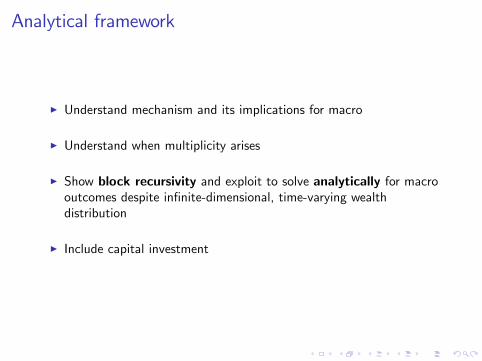
Analytical framework

I Understand mechanism and its implications for macro

I Understand when multiplicity arises

I Show block recursivity and exploit to solve analytically for macrooutcomes despite in�nite-dimensional, time-varying wealthdistribution

I Include capital investment

Large implications for macro outcomes

1. Emergence Unemployment Trap

2. Breakdown Taylor Principle

3. Ampli�cation Mechanism (Employment & Investment)

4. Tightness - Real Interest Rate Nexus

5. In�ationary Impact Productivity Shocks

6. Sources of ZLB

7. Missing De�ation at the ZLB

8. Overturn Supply Shock Paradox

9. Endogenous Risk Premia

! All derive from endogenous countercyclical risk due toHANK+SAM

Literature

I HANK: Gali, Lopez-Salido and Valles (2004), Bilbiie (2008), Auclert(2015), Bayer, Pham-Dao, Luetticke and Tjaden (2015), Beaudry,Galizia and Portier (2014), Challe, Matheron, Ragot andRubio-Ramirez (2016), Heathcote and Perri (2015), Werning (2015),Gornemann, Kuester and Nakajima (2016), Guerrieri and Lorenzoni(2016), Kaplan, Moll and Violante (2016), Luetticke (2015), McKay,Nakamura and Steinsson (2016), McKay and Reis (2016), Bilbiieand Ragot (2016), Farhi and Werning (2017), Auclert and Rognlie(2017), Hagedorn, Manovskii and Mitman (2017), Hedlund,Mitman, Karahan and Ozkan (2017), Legrand and Ragot (2017),Farhi and Werning (2017), etc. etc.

I HANK & SAM: Ravn and Sterk (2012), Challe, Matheron, Ragotand Rubio-Ramirez (2014), Berger, Dew-Becker, Schmidt andTakahasi (2016), Den Haan, Rendahl and Riegler (2015), Kekre(2015), McKay and Reis (2016), Auclert and Rognlie (2017), Challe(2017), etc. etc.

Preferences

I continuum of single-member households, indexed by i 2 [0, 1]I utility:

Vi ,t = Et

∞

∑s=t

βs�t c1�σi ,s � 11� σ

� ζni ,s

!,

I consumption:

ci ,s =�Z

j

�c ji ,s

�1�1/γdj�1/(1�1/γ)

I employment status:

ni ,s =�0 if not employed at date s1 if employed at date s

I receive wi ,s when employed, produce ϑ at home if not employed

Production technology

I production technology of �rm j :

yj ,s = exp (As ) kµj ,sn

1�µj ,s

nj ,s = (1�ω)nj ,s�1 + hj ,skj ,s = (1� δ)kj ,s�1 + ij ,s

I Firm owns stock of physical capital (kj ) employee capital (nj )

I TFP (As ) follows AR(1)

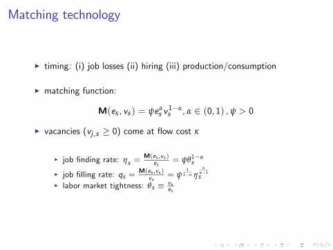
Matching technology

I timing: (i) job losses (ii) hiring (iii) production/consumption

I matching function:

M(es , vs ) = ψeαs v1�αs , α 2 (0, 1) ,ψ > 0

I vacancies (vj ,s � 0) come at �ow cost κ

I job �nding rate: ηs =M(es ,vs )

es= ψθ1�α

s

I job �lling rate: qs =M(es ,vs )

vs= ψ

11�α η

αα�1s

I labor market tightness: θs � vses

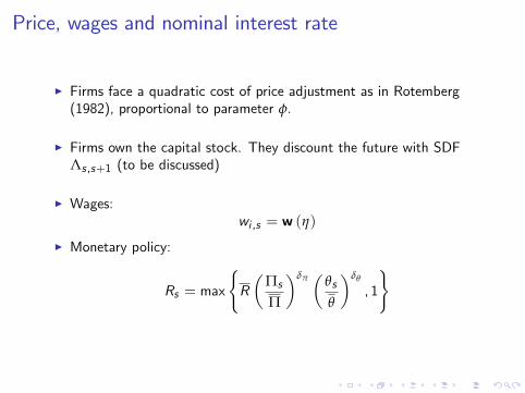
Price, wages and nominal interest rate

I Firms face a quadratic cost of price adjustment as in Rotemberg(1982), proportional to parameter φ.

I Firms own the capital stock. They discount the future with SDFΛs ,s+1 (to be discussed)

I Wages:wi ,s = w (η)

I Monetary policy:

Rs = max

(R�

Πs

Π

�δπ�

θs

θ

�δθ

, 1

)

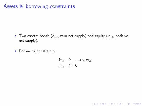
Assets & borrowing constraints

I Two assets: bonds (bi ,s , zero net supply) and equity (xi ,s , positivenet supply).

I Borrowing constraints:

bi ,s � �{wsni ,sxi ,s � 0

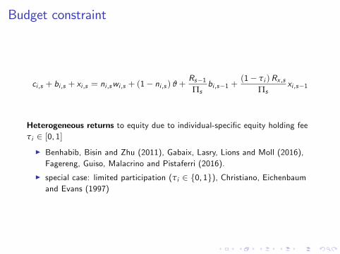
Budget constraint

ci ,s + bi ,s + xi ,s = ni ,swi ,s + (1� ni ,s ) ϑ+Rs�1Πs

bi ,s�1 +(1� τi )Rx ,s

Πsxi ,s�1

Heterogeneous returns to equity due to individual-speci�c equity holding feeτi 2 [0, 1]I Benhabib, Bisin and Zhu (2011), Gabaix, Lasry, Lions and Moll (2016),Fagereng, Guiso, Malacrino and Pistaferri (2016).

I special case: limited participation (τi 2 f0, 1g), Christiano, Eichenbaumand Evans (1997)

Steady state: limited participationequity demand

real return on equity (Rx)

equ

ity

dem

and

0Rx=1/β

supply

asset-poor, employed (τ=1,n=1)

asset-rich (τ=0,n=0)

asset-poor, unemployed (τ=1,n=0)

I Households with τi = 1 do not invest in equity and becomeasset-poor

I Households with τi = 0 hold equity become asset-rich (assume richenough to drop out of labor force).

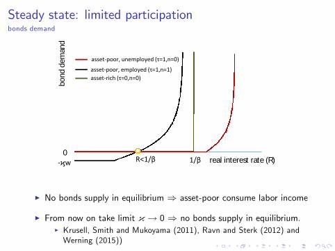
Steady state: limited participationbonds demand

real interest rate (R)

bo

nd

dem

and

0R<1/β-ϗw 1/β

asset-poor, employed (τ=1,n=1)

asset-rich (τ=0,n=0)

asset-poor, unemployed (τ=1,n=0)

I No bonds supply in equilibrium ) asset-poor consume labor income

I From now on take limit { ! 0 ) no bonds supply in equilibrium.I Krusell, Smith and Mukoyama (2011), Ravn and Sterk (2012) andWerning (2015))

Steady state: general case

I Equity fee τi follows some distribution with support [0, 1].

I There is a threshold τ such that households with τi > τ do notinvest in equity and end up holding zero wealth in equilibrium

I ) ci ,s = ni ,sws + (1� ni ,s ) ϑ

I Let I = fi : τi > τ, ni ,s = 1g be the set of households who neverinvest in equity and are currently employed.

I Can show that, in equilibrium, these households are on their Eulerequation, i.e.

1 = βRΠ

Es

�ci ,sci ,s+1

�σ

, i 2 I

� βRΠ

Es

�ci ,sci ,s+1

�σ

, i /2 I

Steady state: general case

I Return on equity observed from Euler equation for those withτi = 0:

Rx/Π = 1/β

I All equity investors agree that �rms�discount factor should be

Λs ,s+1 = β

Block recursivity

Macro block 1 (R,Π, η):

1 = βRΠ Θ(η) (EE)

1� γ+ γmc(η) = φ(1� β)(Π� 1)Π (PC)

R = maxfR�Π/Π

�δπ (η/η)δθ1�α , 1g

Block recursivity

Macro block 1 (R,Π, η):

1 = βRΠ Θ(η) (EE)

1� γ+ γmc(η) = φ(1� β)(Π� 1)Π (PC)

R = maxfR�Π/Π

�δπ (η/η)δθ1�α , 1g

where

Θ(η) � 1+ω (1� η)h(w (η) /ϑ)�σ � 1

i� 1

mc(η) � w (η) +(κηα/(1�α)�λf )(1� β(1�ω)1β � 1+ δ

η � η,λf � 0,λf η = 0

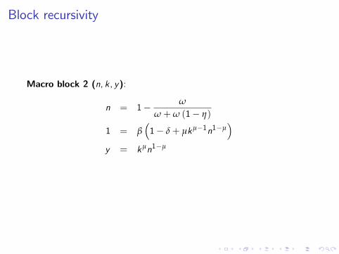
Block recursivity

Macro block 2 (n, k, y):

n = 1� ω

ω+ω (1� η)

1 = β�1� δ+ µkµ�1n1�µ

�y = kµn1�µ

Block recursivity

Distribution block (ci , xi ,Rx ):

c�σi ,s = β

(1� τi )RxΠ

Es c�σi ,s+1 + λx ,i ,s

ci ,s + xi ,s = ni ,swi ,s + (1� ni ,s ) ϑ+(1� τi )Rx ,s

Πsxi ,s�1

xi ,s � 0,λx ,i ,s � 0,λx ,i ,sxi ,s = 0...

for each agent i .

) potentially large amount of wealth heterogeneity

Endogenous vs exogenous risk

I Can express Euler equation (with sticky wage) as:

1 = βRΠ

Θ(pEU )

Θ(pEU ) � 1+ pEUh(w/ϑ)�σ � 1

i� 1

where pEU = ω (1� η) is the employment-to-unemploymenttransition rate.

I In the model pEU = ω (1� η) is endogenousI ) endogenous risk ) endogenous wedge Θ(pEU )

I Alternative assumption: treat pEU as exogenous.I ) exogenous risk ) exogenous wedge Θ(pEU )I constant precautionary savings motive, see also Werning (2015)

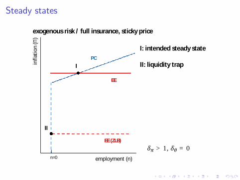
Steady states

3 cases:

I endogenous risk + �exible prices

I exogenous risk + sticky prices

I endogenous risk + sticky prices (baseline)

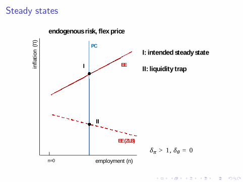
Steady states

I: intended steady state

II: liquidity trap

employment (n)

infl

atio

n(Π

)

II

I

PC

EE (ZLB)

EE

గߜ > 1, ఏߜ = 0

n=0

endogenous risk, flex price

Steady states

I: intended steady state

II: liquidity trap

employment (n)

infl

atio

n(Π

)

I

II

EE

PC

EE (ZLB)

exogenous risk / full insurance, sticky price

n=0

గߜ > 1, ఏߜ = 0

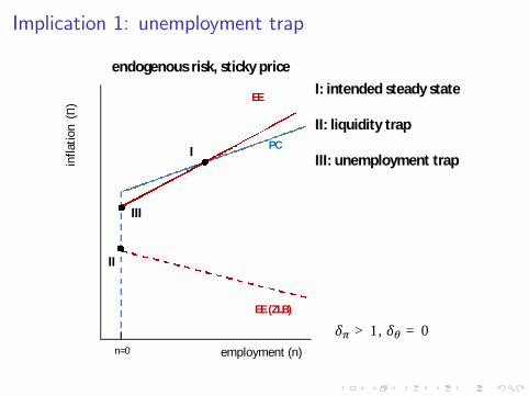
Implication 1: unemployment trap

I: intended steady state

II: liquidity trap

III: unemployment trapinfl

atio

n(Π

)

employment (n)

EE

EE (ZLB)

PCI

II

III

endogenous risk, sticky price

n=0

గߜ > 1, ఏߜ = 0

Dynamics

I Consider local dynamics around intended steady state.

I For sake of simple formulas, assume δπ =1β > 1 (satis�es Taylor

principle), µ = 0 (no capital), and Λs ,s+1 = β

I will all be relaxed

I Again, exploit block recursivity ) in�nite-dimensional,time-varying wealth distribution in the background

I Log-linearize macro block

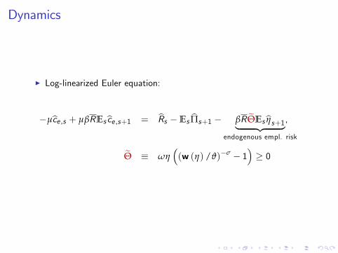
Dynamics

I Log-linearized Euler equation:

�µbce ,s + µβREsbce ,s+1 = bRs �Es bΠs+1 � βR eΘEsbηs+1| {z },endogenous empl. risk

eΘ � ωη�(w (η) /ϑ)�σ � 1

�� 0

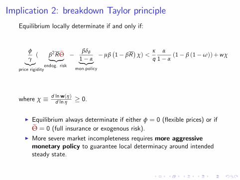
Implication 2: breakdown Taylor principle

Equilibrium locally determinate if and only if:

φ

γ|{z}(price rigidity

β2R eΘ| {z }endog. risk

� βδθ

1� α| {z }mon.policy

�µβ�1� βR

�χ) <

κ

qα

1� α(1� β (1�ω))+wχ

where χ � d lnw(η)d ln η � 0.

I Equilibrium always determinate if either φ = 0 (�exible prices) or ifeΘ = 0 (full insurance or exogenous risk).I More severe market incompleteness requires more aggressivemonetary policy to guarantee local determinacy around intendedsteady state.

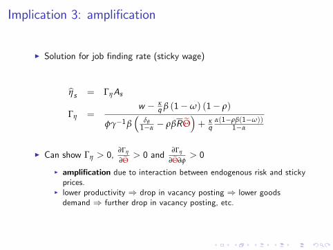
Implication 3: ampli�cation

I Solution for job �nding rate (sticky wage)

bηs = ΓηAs

Γη =w � κ

q β (1�ω) (1� ρ)

φγ�1β�

δθ1�α � ρβR eΘ�+ κ

qα(1�ρβ(1�ω))

1�α

I Can show Γη > 0,∂Γη

∂eΘ > 0 and∂Γη

∂eΘ∂φ> 0

I ampli�cation due to interaction between endogenous risk and stickyprices.

I lower productivity ) drop in vacancy posting ) lower goodsdemand ) further drop in vacancy posting, etc.

Implication 3: ampli�cation

I Now include capitalI further ampli�cation or dampening?

I Also explore di¤erent assumptions on �rms�discount factorsI real interest rate vs subjective discount rate

Calibration

I Monthly model

Steady-state targetsu 0.05 unemployment rateη 0.3 job �nding rate

κψ3w 0.05 hiring cost as fraction of quarterly wage

6 avg. price duration (Calvo equivalent)1� ϑ

w 0.15 income loss upon unemploymentΠ 1 gross in�ation rateR12 � 1 0.03 annual net interest ratek12y 2 ratio capital to annual output

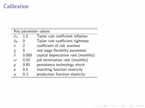
Calibration

Key parameter valuesδπ 1.5 Taylor rule coe¢ cient in�ationδθ 0 Taylor rule coe¢ cient tightnessσ 2 coe¢ cient of risk aversionχ 0 real wage �exibility parameterδ 0.005 capital depreciation rate (monthly)ω 0.02 job termination rate (monthly)ρ 0.85 persistence technology shockα 0.5 matching function elasticityµ 0.3 production function elasticity

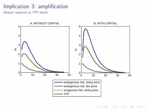
Implication 3: ampli�cationOutput response to TFP shock

0 10 20 30 400

1

2

3

4

5A. WITHOUT CAPITAL

%

0 10 20 30 400

1

2

3

4

5B. WITH CAPITAL

%

endogenous risk, sticky price

endogenous risk, flex price

exogenous risk, sticky price

TFP

Implication 4: nexus between real rate and tightness

bR rs = (1� α)��µχ+

�µχ+ eΘ� βRρ

�bθswhere bR rs � bRs �Es bΠs+1.

I Negative co-movement with exogenous risk or full insurance(eΘ = 0). Positive co-movement between tightness and realinterest rate if eΘ large enough.

I Tight labor market ) low unemployment risk ) weakprecautionary savings motive ) high real interest rate

Implication 4: nexus between real rate and tightness

1990 1995 2000 2005 2010-5

0

5x 10

-3

reali

nte

restra

te(log

poin

ts)

1990 1995 2000 2005 2010-1.5

0

1.5

v-u

ratio

(log

poin

ts)

Real interest rate and labor market tightness (vacancy-unemployment ratio); deviations from trend. The real interest rate computed as the

Federal Funds rate minus a six-month moiving average of CPI in�ation. Vacancies are measured as the composite Help Wanted index

from Barnichon (2010). Data series were logged and de-trended using a linear trend estimated over the period up to the end of 2007.

Implication 5: in�ationary productivity shocks

Solution for in�ation: bΠs = ΓΠAs ,

where

ΓΠ =β2R eΘρ� βδθ

1�α

1� βρΓη

I Note: ΓΠ < 0 under complete markets (eΘ = 0).

I A positive productivity shock is in�ationary if endogenous riskchannel su¢ ciently strong, i.e. if βR eΘρ > δθ

1�α

I Higher productivity ) higher employment ) weaker precautionarysavings motive ) higher goods demand ) in�ationary pressure

Implication 5: in�ationary productivity shocks

response to TFP0

0 5 10 15 20

-0.3

-0.2

-0.1

0

0.1

0.2

0.3

response to TFP1

0 5 10 15 20

-0.3

-0.2

-0.1

0

0.1

0.2

0.3

Notes: IRF of 400*log(cpit/cpit-1) to change in log TFP as estimated by Fernald (2016) using local projection. The sample starts in 1980

and we included 4 lags. TFP0 (TFP1) refers to Fernald estimate for Total Factor Productivity without (with) control for factor utilization.

Shaded areas denote error bands of two standard deviations.

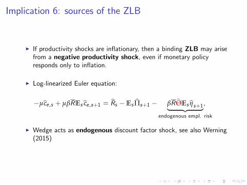
Implication 6: sources of the ZLB

I If productivity shocks are in�ationary, then a binding ZLB may arisefrom a negative productivity shock, even if monetary policyresponds only to in�ation.

I Log-linearized Euler equation:

�µbce ,s + µβREsbce ,s+1 = bRs �Es bΠs+1 � βR eΘEsbηs+1| {z },endogenous empl. risk

I Wedge acts as endogenous discount factor shock, see also Werning(2015)

Implication 7: missing de�ation at the ZLB

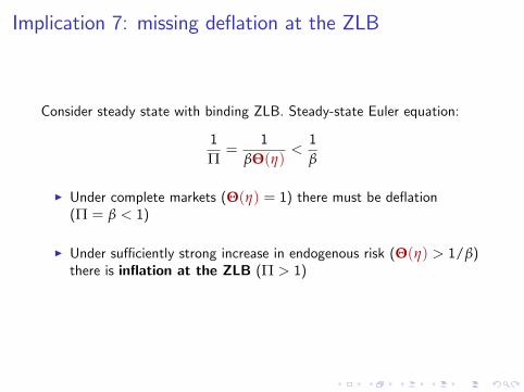
Implication 7: missing de�ation at the ZLB

Consider steady state with binding ZLB. Steady-state Euler equation:

1Π=

1βΘ(η)

<1β

I Under complete markets (Θ(η) = 1) there must be de�ation(Π = β < 1)

I Under su¢ ciently strong increase in endogenous risk (Θ(η) > 1/β)there is in�ation at the ZLB (Π > 1)

Implication 8: supply shock paradox at the ZLB

I Endogenous risk can overturn the paradox that a positiveproductivity shock creates an economic contraction at the ZLB(Eggertsson, 2010):

I Assume ZLB persists with probability p.

I Slope (log-linearized) EE curve: dbΠsdbηs = µχ

p

�1� βRp

�� βR eΘ

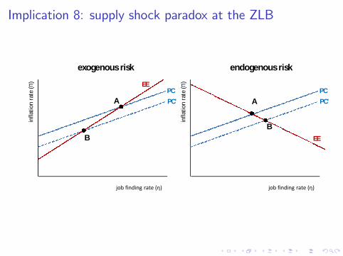
Implication 8: supply shock paradox at the ZLBin

flat

ion

rate

(Π)

job finding rate (η)

EE

PC’

B

exogenous risk

A

PC

infl

atio

nra

te(Π

)job finding rate (η)

EE

PC’

B

endogenous risk

A

PC

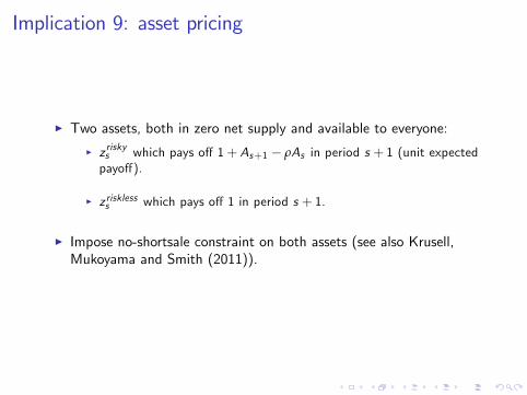
Implication 9: asset pricing

I Two assets, both in zero net supply and available to everyone:

I z riskys which pays o¤ 1+ As+1 � ρAs in period s + 1 (unit expectedpayo¤).

I z risklesss which pays o¤ 1 in period s + 1.

I Impose no-shortsale constraint on both assets (see also Krusell,Mukoyama and Smith (2011)).

Implication 9: asset pricing

I Price di¤erence (based on log-linearized model) given by:

z risklesss � z riskys = βeΘΓησ2A

I Positive risk premium due to endogenous risk (eΘ > 0).

I Monetary policy a¤ects risk premium via Γη

Conclusion

I Analytically tractable HANK model with endogenous employmentrisk

I Feedback between precautionary saving and the demand for goodsand labor creates strong destabilizing force

I highlighted nine major implications for macroI can be addressed by stabilization policy

I Analytical solutions for macro outcomes despite time-varying wealthdistribution

I thanks to block recursivityI next step: solve for dynamics of wealth distribution

Appendix

Labor force participation in general case

I Given that households with τi = 0 withdraw from the labor force,any household with τi > 0 will be in labor force. The Euler equationfor equity implies that:

c�σi ,s

Esc�σi ,s+1

= βRxΠ(1� τi )

= (1� τi ) � 1

which holds with strict inequality if τi > 0.I Thus any household out of the labor force with τi > 0 will satisfyci ,s+1ci ,s

< 1 i.e. have a strictly declining consumption pro�le. Thehousehold eats into its savings.

I At some point, consumption of the household will be low that thehousehold will be back in the labor force.

I When back in the labor force, the precautionary motive kicks in,which implies that Esci ,s+1 > ci ,s .

Role of �rms�discountingOutput response to TFP shock

0 10 20 30 400

1

2

3

4

5A. WITHOUT CAPITAL

%

0 10 20 30 400

1

2

3

4

5B. WITH CAPITAL

%firms discount with subjective discount rate (1/)

firms discount with real interest rate (Es[R

s/

s+1])

TFP