morphodig user's guide morphodig v1.6
TRANSCRIPT

MorphoDig User's guide
MorphoDig v1.6.0
Renaud LEBRUN
Institut des Sciences de l'Evolution, University of Montpellier, France
Montpellier Ressources Imaging platform
December 17, 2020

2
Contents
Introduction 7
Origin of the project . . . . . . . . . . . . . . . . . . . . . . . . . . . . . . . . . . . . 7
Main features . . . . . . . . . . . . . . . . . . . . . . . . . . . . . . . . . . . . . . . . 7
Implementation . . . . . . . . . . . . . . . . . . . . . . . . . . . . . . . . . . . . . . . 8
1 Licence 9
1.1 MorphoDig . . . . . . . . . . . . . . . . . . . . . . . . . . . . . . . . . . . . . . 9
1.2 VTK . . . . . . . . . . . . . . . . . . . . . . . . . . . . . . . . . . . . . . . . . . 9
2 F.A.Q. 11
2.1 How should I cite MorphoDig in scienti�c publications ? . . . . . . . . . . . . . 11
2.2 Is MorphoDig a geometric morphometrics software ? . . . . . . . . . . . . . . . . 11
2.3 Can I produce/extract 3D surfaces (meshes) out of CT/MRI data using Mor-phoDig ? . . . . . . . . . . . . . . . . . . . . . . . . . . . . . . . . . . . . . . . . 12
2.4 Is there a CTRL-Z functionality ? . . . . . . . . . . . . . . . . . . . . . . . . . . 12
3 Main window, Open data, Save data, Undo-Redo actions 13
3.1 Main window. . . . . . . . . . . . . . . . . . . . . . . . . . . . . . . . . . . . . . 13
3.2 Open and save data . . . . . . . . . . . . . . . . . . . . . . . . . . . . . . . . . . 13
3.3 Undo-Redo actions . . . . . . . . . . . . . . . . . . . . . . . . . . . . . . . . . . 15
4 Interactions and color display. 17
4.1 Interacting with objects . . . . . . . . . . . . . . . . . . . . . . . . . . . . . . . 17
4.2 Interactions modes . . . . . . . . . . . . . . . . . . . . . . . . . . . . . . . . . . 18
4.3 Landmark setting modes . . . . . . . . . . . . . . . . . . . . . . . . . . . . . . . 18
4.4 Unselected surfaces color display . . . . . . . . . . . . . . . . . . . . . . . . . . . 20
5 Keyboard and mouse controls 23
5.1 Keyboard and mouse controls . . . . . . . . . . . . . . . . . . . . . . . . . . . . 25
5.2 Additional controls . . . . . . . . . . . . . . . . . . . . . . . . . . . . . . . . . . 26
3

4 CONTENTS
6 Main window controls 276.1 Camera controls . . . . . . . . . . . . . . . . . . . . . . . . . . . . . . . . . . . . 286.2 Display controls . . . . . . . . . . . . . . . . . . . . . . . . . . . . . . . . . . . . 316.3 Object controls . . . . . . . . . . . . . . . . . . . . . . . . . . . . . . . . . . . . 34
7 Menu File 457.1 Project . . . . . . . . . . . . . . . . . . . . . . . . . . . . . . . . . . . . . . . . . 477.2 Surface . . . . . . . . . . . . . . . . . . . . . . . . . . . . . . . . . . . . . . . . . 507.3 Position . . . . . . . . . . . . . . . . . . . . . . . . . . . . . . . . . . . . . . . . 537.4 Landmarks . . . . . . . . . . . . . . . . . . . . . . . . . . . . . . . . . . . . . . 567.5 Curves . . . . . . . . . . . . . . . . . . . . . . . . . . . . . . . . . . . . . . . . . 597.6 Flags . . . . . . . . . . . . . . . . . . . . . . . . . . . . . . . . . . . . . . . . . . 647.7 Color maps . . . . . . . . . . . . . . . . . . . . . . . . . . . . . . . . . . . . . . 657.8 Tag maps . . . . . . . . . . . . . . . . . . . . . . . . . . . . . . . . . . . . . . . 667.9 Orientation helper labels . . . . . . . . . . . . . . . . . . . . . . . . . . . . . . . 687.10 Measurements . . . . . . . . . . . . . . . . . . . . . . . . . . . . . . . . . . . . . 687.11 Volume . . . . . . . . . . . . . . . . . . . . . . . . . . . . . . . . . . . . . . . . . 72
8 Menu Edit 798.1 Edit color and lighting options . . . . . . . . . . . . . . . . . . . . . . . . . . . . 798.2 Edit size unit, grid spacing and scale . . . . . . . . . . . . . . . . . . . . . . . . 808.3 Landmark and �ag rendering options . . . . . . . . . . . . . . . . . . . . . . . . 828.4 Edit orientation labels . . . . . . . . . . . . . . . . . . . . . . . . . . . . . . . . 838.5 Edit camera options . . . . . . . . . . . . . . . . . . . . . . . . . . . . . . . . . 868.6 Volume options . . . . . . . . . . . . . . . . . . . . . . . . . . . . . . . . . . . . 868.7 Renderer options . . . . . . . . . . . . . . . . . . . . . . . . . . . . . . . . . . . 86
9 Menu Surfaces 899.1 Edit �rst selected surface . . . . . . . . . . . . . . . . . . . . . . . . . . . . . . . 909.2 Structure modi�cation . . . . . . . . . . . . . . . . . . . . . . . . . . . . . . . . 909.3 Wrapping methods . . . . . . . . . . . . . . . . . . . . . . . . . . . . . . . . . . 1019.4 Boolean operations . . . . . . . . . . . . . . . . . . . . . . . . . . . . . . . . . . 1039.5 Surface alignment . . . . . . . . . . . . . . . . . . . . . . . . . . . . . . . . . . . 1059.6 Rendering modi�cation . . . . . . . . . . . . . . . . . . . . . . . . . . . . . . . . 1069.7 Create 3D primitives . . . . . . . . . . . . . . . . . . . . . . . . . . . . . . . . . 1069.8 Select small objects . . . . . . . . . . . . . . . . . . . . . . . . . . . . . . . . . . 1129.9 Select small volumes . . . . . . . . . . . . . . . . . . . . . . . . . . . . . . . . . 112
10 Menu Landmarks 11510.1 Edit �rst selected landmark . . . . . . . . . . . . . . . . . . . . . . . . . . . . . 11610.2 Edit �rst selected �ag . . . . . . . . . . . . . . . . . . . . . . . . . . . . . . . . . 116

CONTENTS 5
10.3 Select landmark range . . . . . . . . . . . . . . . . . . . . . . . . . . . . . . . . 11710.4 Selected landmarks: decrease landmark number (move up in list) . . . . . . . . . 11810.5 Selected landmarks: increase landmark number (move down in list) . . . . . . . 11810.6 Selected landmarks: push back on closest surface's vertex . . . . . . . . . . . . . 11810.7 Selected landmarks: change orientation according to surface's normals . . . . . . 11810.8 Selected curve nodes and curve handle landmarks . . . . . . . . . . . . . . . . . 12010.9 Edit color of all selected �ag landmarks . . . . . . . . . . . . . . . . . . . . . . . 12410.10Edit length of all selected �ag landmarks . . . . . . . . . . . . . . . . . . . . . . 12410.11Update all selected �ag landmarks' color to that of the closest vertex . . . . . . 124
11 Menu Scalars 12711.1 Open scalars window . . . . . . . . . . . . . . . . . . . . . . . . . . . . . . . . . 12811.2 Compute distance from camera for each selected surface . . . . . . . . . . . . . . 13111.3 Compute thickness within each selected surface . . . . . . . . . . . . . . . . . . 13611.4 Compute thickness between two surfaces . . . . . . . . . . . . . . . . . . . . . . 13711.5 Compute distance between two surfaces . . . . . . . . . . . . . . . . . . . . . . . 13811.6 Compute curvature for each selected surface . . . . . . . . . . . . . . . . . . . . 13811.7 Compute complexity for each selected surface . . . . . . . . . . . . . . . . . . . 13911.8 Smooth active scalars for each selected surface . . . . . . . . . . . . . . . . . . . 14411.9 Normalize or rescale active scalars for each selected surface . . . . . . . . . . . . 144
12 Menu Tags 15112.1 Open Tags window . . . . . . . . . . . . . . . . . . . . . . . . . . . . . . . . . . 15212.2 Create new empty tag array for each selected surface . . . . . . . . . . . . . . . 15212.3 Create new tag array based on currently displayed colors for each selected surface15212.4 Create new tag array based on connectivity for each selected surface . . . . . . . 15512.5 Extract active tag region for each selected surface . . . . . . . . . . . . . . . . . 15512.6 Extract tag region range for each selected surface . . . . . . . . . . . . . . . . . 15512.7 Extract each tag region as a new object, for all tag regions of all selected surfaces15612.8 Tagging with MorphoDig: a quick starting guide . . . . . . . . . . . . . . . . . . 156
13 Menu RGB 16113.1 Create or replace an RGB array with current display color . . . . . . . . . . . . 161
14 Menu Volumes 16314.1 Edit �rst selected volume . . . . . . . . . . . . . . . . . . . . . . . . . . . . . . . 16414.2 Extract isosurface from �rst selected volume . . . . . . . . . . . . . . . . . . . . 17514.3 Flip or swap �rst selected volume . . . . . . . . . . . . . . . . . . . . . . . . . . 17514.4 Change voxel size of �rst selected volume (keep dimensions, no resampling . . . 17514.5 Resample �rst selected volume (dimensions will be changed, and voxel size as well)18114.6 Reslice �rst selected volume . . . . . . . . . . . . . . . . . . . . . . . . . . . . . 181

6 CONTENTS
14.7 Median �lter of �rst selected volume . . . . . . . . . . . . . . . . . . . . . . . . 18314.8 Gaussian �lter of �rst selected volume . . . . . . . . . . . . . . . . . . . . . . . 18314.9 Invert �rst selected volume . . . . . . . . . . . . . . . . . . . . . . . . . . . . . . 183
15 View 189
16 Help 19116.1 MorphoDig Web Site . . . . . . . . . . . . . . . . . . . . . . . . . . . . . . . . . 19116.2 MorphoDig Tutorials . . . . . . . . . . . . . . . . . . . . . . . . . . . . . . . . . 19116.3 About... . . . . . . . . . . . . . . . . . . . . . . . . . . . . . . . . . . . . . . . . 191
17 Acknowledgments 19317.1 Design concepts . . . . . . . . . . . . . . . . . . . . . . . . . . . . . . . . . . . . 19317.2 Code development . . . . . . . . . . . . . . . . . . . . . . . . . . . . . . . . . . 19317.3 Specimens illustrated . . . . . . . . . . . . . . . . . . . . . . . . . . . . . . . . . 19317.4 3D data acquisition facilities . . . . . . . . . . . . . . . . . . . . . . . . . . . . . 194
References 195

Introduction
ContentsOrigin of the project . . . . . . . . . . . . . . . . . . . . . . . . . . . . . . . 7
Main features . . . . . . . . . . . . . . . . . . . . . . . . . . . . . . . . . . . 7
Implementation . . . . . . . . . . . . . . . . . . . . . . . . . . . . . . . . . . 8
MorphoDig is based on the design concepts of the software FoRM-IT (Fossil Reconstructionand Morphometry Interactive Toolkit; [Zollikofer and Ponce de León, 1995, 2005]). Mor-phoDig[Lebrun, 2018] was developed as a help to the scienti�c journal MorphoMuseuM (M3),in order to help scientists to produce enriched surface models. MorphoDig also opens 3D volumedata such as CT datasets. The source code is hosted on Github.
Origin of the project
Over the last two decades, even though 3D data acquisition and computer-assisted techniqueshave grown increasingly popular among biologists, paleontologists and paleoanthropologists,so far, no standard biology-oriented 3D mesh manipulation software has emerged; most of thetime, researchers either use commercial software which are not primarily designed for biologists,or develop their own in-house software solutions. MorphoDig builds upon the design concepts ofthe software FoRM-IT (Fossil Reconstruction and Morphometry Interactive Toolkit; [Zollikoferand Ponce de León, 1995, 2005]), and is developed to meet the need to ease the productionand the di�usion of 3D models of biological organisms. MorphoDig provides a set of tools forediting, positioning, deforming, labeling, tagging sets of 3D surfaces. As such, MorphoDig canbe used to produce enriched models which can in turn be submitted to M3. Since version 1.5,MorphoDig also provides tool for opening, editing and visualizing 3D volumes, and to extract3D surfaces out of 3D volumes.
Main features
Features include:
7

8
• Retro-deformation for virtual restoration of fossils/deformed specimens;
• Point and curve primitives for placing the exact type of landmark points you're interestedin
• Easy to use 3D interface for positioning and manipulating sets of surfaces and landmarkprimitives
• Surface tagging, labeling and coloring (to allow for the creation of anatomy atlases)
• Surface scalar computation and coloring (based upon curvature/thickness etc...)
• Volume rendering of CT data (3D Volumes).
• Isosurface extraction from CT data.
• 3D Mask edition.
MorphoDig allows to import and export 3D meshes in standard formats such as STL, PLYand VTK polydata, and as such, in can be used in conjunction with a variety of other 3D mesheditors such as MeshLab (http://meshlab.sourceforge.net/) or Blender (https://www.blender.org/).MorphoDig also allows to import 3D volume in standard formats such as DICOM, TIFF, BMP,PNG, Meta-Image and RAW.
Implementation
MorphoDig is entirely written in C++, and uses the visualization library VTK [Avila et al.,2001]. The GUI has been designed with QT (https://www.qt.io/). MorphoDig is open-sourceand cross platform, and we are looking forward to welcoming new developers in the future inorder to implement new functionalities.

Chapter 1
Licence
Contents1.1 MorphoDig . . . . . . . . . . . . . . . . . . . . . . . . . . . . . . . . . 9
1.2 VTK . . . . . . . . . . . . . . . . . . . . . . . . . . . . . . . . . . . . . 9
1.1 MorphoDig
MorphoDig is Copyright(C) 2018: CNRS, Renaud LEBRUN. All rights reserved. MorphoDigis an open-source software licensed under the BSD Licence.
Redistribution and use in source and binary forms, with or without modi�cation, are per-mitted provided that the following conditions are met:
Re-distributions of source code must retain the above copyright notice, this list of conditionsand the following disclaimer.
Re-distributions in binary form must reproduce the above copyright notice, this list ofconditions and the following disclaimer in the documentation and/or other materials providedwith the distribution.
1.2 VTK
MorphoDig's compiled versions contain binary forms of VTK: Copyright (c) 2000-2006 KitwareInc. 28 Corporate Drive, Suite 204, Clifton Park, NY, 12065, USA. All rights reserved. Re-distribution and use in source and binary forms, with or without modi�cation, are permitted
9

10 1.2. VTK
provided that the following conditions are met:Redistributions of source code must retain the above copyright notice, this list of conditionsand the following disclaimer.Redistributions in binary form must reproduce the above copyright notice, this list of conditionsand the following disclaimer in the documentation and/or other materials provided with thedistribution.Neither the name of Kitware nor the names of any contributors may be used to endorse orpromote products derived from this software without speci�c prior written permission.
THIS SOFTWARE IS PROVIDED BY THE COPYRIGHT HOLDERS AND CONTRIB-UTORS �AS IS" AND ANY EXPRESS OR IMPLIED WARRANTIES, INCLUDING, BUTNOT LIMITED TO, THE IMPLIED WARRANTIES OF MERCHANTABILITY AND FIT-NESS FOR A PARTICULAR PURPOSE ARE DISCLAIMED. IN NO EVENT SHALL THEAUTHORS OR CONTRIBUTORS BE LIABLE FOR ANY DIRECT, INDIRECT, INCIDEN-TAL, SPECIAL, EXEMPLARY, OR CONSEQUENTIAL DAMAGES (INCLUDING, BUTNOT LIMITED TO, PROCUREMENT OF SUBSTITUTE GOODS OR SERVICES; LOSSOF USE, DATA, OR PROFITS; OR BUSINESS INTERRUPTION) HOWEVER CAUSEDAND ON ANY THEORY OF LIABILITY, WHETHER IN CONTRACT, STRICT LIABIL-ITY, OR TORT (INCLUDING NEGLIGENCE OR OTHERWISE) ARISING IN ANY WAYOUT OF THE USE OF THIS SOFTWARE, EVEN IF ADVISED OF THE POSSIBILITYOF SUCH DAMAGE.

Chapter 2
F.A.Q.
Contents2.1 How should I cite MorphoDig in scienti�c publications ? . . . . . . 11
2.2 Is MorphoDig a geometric morphometrics software ? . . . . . . . . 11
2.3 Can I produce/extract 3D surfaces (meshes) out of CT/MRI datausing MorphoDig ? . . . . . . . . . . . . . . . . . . . . . . . . . . . . 12
2.4 Is there a CTRL-Z functionality ? . . . . . . . . . . . . . . . . . . . 12
2.1 How should I cite MorphoDig in scienti�c publications
?
You may cite MorphoDig with the following reference :Lebrun, R. MorphoDig, an open-source 3D freeware dedicated to biology. IPC5, Paris, France;07/2018.
2.2 Is MorphoDig a geometric morphometrics software ?
No. However, you can digitize 3D landmarks on complex 3D surfaces or on 3D volume renderingrepresentations using MorphoDig, which you can use in other software.
11

122.3. CAN I PRODUCE/EXTRACT 3D SURFACES (MESHES) OUT OF CT/MRI DATA
USING MORPHODIG ?
2.3 Can I produce/extract 3D surfaces (meshes) out of
CT/MRI data using MorphoDig ?
Currently, the only possibility to produce a surface with MorphoDig is, using a given thresholdvalue, to create an isosurface (using the marching cubes algorithm, for instance). Segmentationtools will be added in future versions of this software.
2.4 Is there a CTRL-Z functionality ?
Yes, de�nitely. Most actions can be undone and redone.

Chapter 3
Main window, Open data, Save data,
Undo-Redo actions
Contents3.1 Main window. . . . . . . . . . . . . . . . . . . . . . . . . . . . . . . . . 13
3.2 Open and save data . . . . . . . . . . . . . . . . . . . . . . . . . . . . 13
3.3 Undo-Redo actions . . . . . . . . . . . . . . . . . . . . . . . . . . . . . 15
3.1 Main window.
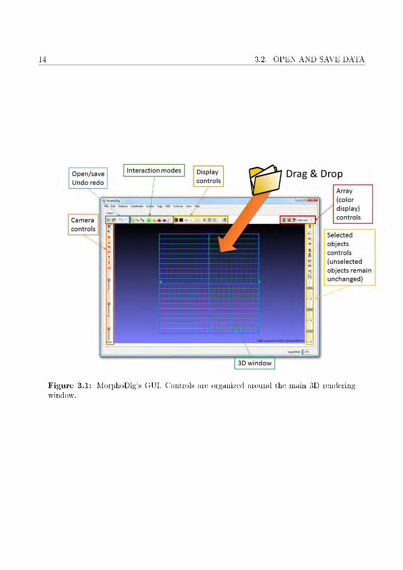
MorphoDig's main window is organized as shown in Fig. 3.1 p.14. The most commonly usedcontrols are directly accessible nearby the main 3D rendering window, and are sorted by func-tion.
3.2 Open and save data
• There are three main ways to open data in MorphoDig. First, you can open speci�c �lesvia the menu "File". You may also open data by clicking on the "open" ( ) buttoninside the main window (or press "CTRL +O"). You may also drag and drop �les withinthe main 3D window. STL, PLY and VTK polydata surface �les (.vtk and .vtp �les)can be opened by MorphoDig, and many �les speci�c to that software (�les, curves,positions, color maps, tag maps, orientation-helper labels etc.). MorphoDig also opens3D volumetric data such as .ti� 2D image sequences, .dcm (DICOM) image sequences,3D .ti� �les, 3D .raw �les, and 3D .mhd or .mha �les (meta-image format).
13
14 3.2. OPEN AND SAVE DATA
Figure 3.1: MorphoDig's GUI. Controls are organized around the main 3D renderingwindow.

CHAPTER 3. MAIN WINDOW, OPEN DATA, SAVE DATA, UNDO-REDO ACTIONS 15
• In most cases, only selected objects (or some of their properties) can be saved; most"save" functionalities will not a�ect unselected objects. There are two main ways to savedata in MorphoDig. First, you can save speci�c �les through the menu "File". You mayalso save a project with the button "save project" ( ) inside the main window. Onlyselected objects will be considered when saving a project.
3.3 Undo-Redo actions
• Most actions, such as opening data, deleting data, selecting/unselecting objects, placinglandmarks, modify the position of landmarks/surfaces, surface tagging etc. can be undoneby clicking the "undo" button ( ).
• The same actions can be redone by clicking on the "redo" button ( ).

16 3.3. UNDO-REDO ACTIONS

Chapter 4
Interactions and color display.
Contents4.1 Interacting with objects . . . . . . . . . . . . . . . . . . . . . . . . . 17
4.2 Interactions modes . . . . . . . . . . . . . . . . . . . . . . . . . . . . . 18
4.2.1 Camera mode . . . . . . . . . . . . . . . . . . . . . . . . . . . . . . . . 18
4.2.2 Object mode . . . . . . . . . . . . . . . . . . . . . . . . . . . . . . . . 18
4.2.3 Landmark mode . . . . . . . . . . . . . . . . . . . . . . . . . . . . . . 18
4.3 Landmark setting modes . . . . . . . . . . . . . . . . . . . . . . . . . 18
4.3.1 Normal landmark mode . . . . . . . . . . . . . . . . . . . . . . . . . . 18
4.3.2 Target landmark mode . . . . . . . . . . . . . . . . . . . . . . . . . . . 18
4.3.3 Curve node mode . . . . . . . . . . . . . . . . . . . . . . . . . . . . . . 20
4.3.4 Curve handle mode . . . . . . . . . . . . . . . . . . . . . . . . . . . . . 20
4.3.5 Flag landmark mode . . . . . . . . . . . . . . . . . . . . . . . . . . . . 20
4.4 Unselected surfaces color display . . . . . . . . . . . . . . . . . . . . 20
4.1 Interacting with objects
One very important aspect of MorphoDig's design is that most interactions or modi�cationsof opened objects can only be done when these objects are selected. Selected surfaces (free-form surfaces, landmarks and �ags) are always drawn in �grey". Regarding volumetric objects,selected ones appear with a bounding box, while unselected ones to not exhibit such boundingboxes. See Fig. 4.1 p.19. All currently opened objects can be selected by pressing CTRL+A.All currently opened objects can be unselected by pressing CTRL+D. Objects can also be
17

18 4.2. INTERACTIONS MODES
selected/unselected using the right mouse button, depending on the currently active interactionmode (see below).
4.2 Interactions modes
See Fig. 3.1 p.14 to �nd the location of the "Interaction modes" controls in the main Window.
4.2.1 Camera mode
�Camera mode" is the default interaction mode, and is active on startup. When active,left and middle mouse button drags result in camera rotation/translation, respectively. Rightmouse button drag results in object selection/unselection. Pressing "ESC" switches betweenobject mode and camera mode.
4.2.2 Object mode
When active, left and middle mouse button drags result in object rotation/translation, re-spectively. Right mouse button drag results in object selection/unselection. Pressing "ESC"switches between object mode and camera mode.
4.2.3 Landmark mode
When active, only landmarks can be selected/unselected via right mouse button drag. Thismode is useful when editing/placing landmarks. Left and middle mouse button drags result incamera rotation/translation, respectively.
4.3 Landmark setting modes
Landmarks can be set on surfaces by pressing �L" + left mouse click. Four series of landmarkscan be set with MorphoDig: �normal" landmarks, �target" landmarks, �curve node" landmarksand �curve handle" landmarks. Additionally a fourth special landmark series (��ag" landmarks)can be used to label surface structures.
4.3.1 Normal landmark mode
Press � " to activate this mode (this mode is active by default)
4.3.2 Target landmark mode
Press � " to activate this mode

CHAPTER 4. INTERACTIONS AND COLOR DISPLAY. 19
Figure 4.1: A unselected volumes have no bounding box. B unselected surfaces areusually not drawn grey. C selected volumes exhibit a bounding box. D selected surfacesare drawn grey.

20 4.4. UNSELECTED SURFACES COLOR DISPLAY
4.3.3 Curve node mode
Press � " to activate this mode
4.3.4 Curve handle mode
Press � " to activate this mode
4.3.5 Flag landmark mode
Press � " to activate this mode
4.4 Unselected surfaces color display
See Fig. 3.1 p.14 to �nd the location of the "Array controls", which impact the color displayof the surfaces. A given unselected surface can be colored:
• using a uniform �solid" color (Fig. 4.2-A p.21). Scalar display mode must be deactivated
or active array combo box set to �Solid color" ( )
• according to the scalar values (= numbers) associated at the vertices (Fig. 4.2-B p.21).
Array display mode button must be pressed ( ), and a Scalar array must be selected
(ex: ). The way scalar arrays are translated into colors can be set up using color"Lookup tables" (LUT), also referred to as color transfer functions. The "Scalar rendering
options" window can be opened by clicking on " ".
• according to the tag values (= integers) associated to the vertices (Fig. 4.2-C p.21).
Array display mode button must be pressed ( ), and a Tag array must be selected
(ex: ). The way Tag arrays are translated into colors can be set up using color"Lookup tables" (LUT), also referred to as color transfer functions. The "Tag options"window, in which lookup tables associated to tag arrays can be edited, can be opened by
clicking on " "
• according to RGB values directly associated to the vertices (Fig. 4.2-D p.21). Array
display mode button must be pressed ( ), and a RGB array must be selected (ex: )

CHAPTER 4. INTERACTIONS AND COLOR DISPLAY. 21
Figure 4.2: Color modes for a given surface. Single surface representation of the skeletonof a newborn Lemur catta. A: "Solid color mode" mode : a uniform color is used torepresent the whole surface. B: "Scalar array" representation mode. Numbers (here bonethickness) are associated to each vertex of the surface, and are rendered using a color map.C: "Tag array". Integers are associated to each vertex (here di�erent integer values areassociated to di�erent groups of bones), and a color map is used to colorize the specimen.D : "RGB array" : red, green, blue and transparency information is directly associatedto each vertex: no color map is used in that case. In MorphoDig, RGB arrays can beproduced out of solid color information, scalar arrays and tag arrays. PLY �le producedvia surface scans often contain surch RGB information.

22 4.4. UNSELECTED SURFACES COLOR DISPLAY

Chapter 5
Keyboard and mouse controls
Contents
5.1 Keyboard and mouse controls . . . . . . . . . . . . . . . . . . . . . . 25
5.2 Additional controls . . . . . . . . . . . . . . . . . . . . . . . . . . . . 26
23

24

CHAPTER 5. KEYBOARD AND MOUSE CONTROLS 25
5.1 Keyboard and mouse controls
Ctrl+A Selects all objectsCtrl+D Unselects all objectsCtrl+Z Undo last actionCtrl+Y Redo last action
L+ left click Creates a landmark (either �normal", �target",�curve node", �curve handle" or ��ag" landmark).Warning: this option does not work with touchpads,you need a "real" mouse to be able to combine "T"and a left click (see below for an alternative).
Shift+ left click In curve node digitation mode : creates a new curvestarting node. Otherwise, creates a landmark (either�normal", �target", �curve handle" or ��ag" land-mark). Works with touchpads
J+ left click In curve node digitation mode : creates a new curvemilestone node. Otherwise, creates a landmark (ei-ther �normal", �target", �curve handle" or ��ag"landmark).
K+ left click In curve node digitation mode : creates a new curvenode that will be connected to the preceding startingnode. Otherwise, creates a landmark (either �nor-mal", �target", �curve handle" or ��ag" landmark).
L + right click If a single landmark or �ag is selected, its positionis moved. Nothing happens if no landmark nor �agis selected or if more than one landmark or �ag areselected. Warning: this option does not work withtouchpads, you need a "real" mouse to be able tocombine "T" and a right click.
Shift + right click Same as above, but works with touchpads.Left mouse button drag Camera mode : camera rotation.
Object mode : object rotation.Landmark mode : camera rotation.
Ctrl + left mouse button drag Camera mode : object rotation.Object mode : camera rotation.Landmark mode : object rotation.
Right mouse button drag Draws a yellow rectangle. Once right button is re-leased, all objects (surfaces and landmarks) fallinginside the rectangle get selected/unselected, depend-ing on their initial selection status
Middle mouse button roll (roll wheel) Zoom / unzoomMiddle mouse button drag Camera mode : camera translation
Object mode : object translationLandmark mode : camera translation
Ctrl + middle mouse button drag Camera mode : object translationObject mode : camera translationLandmark mode : object translation
� Del � All selected objects are deleted
26 5.2. ADDITIONAL CONTROLS
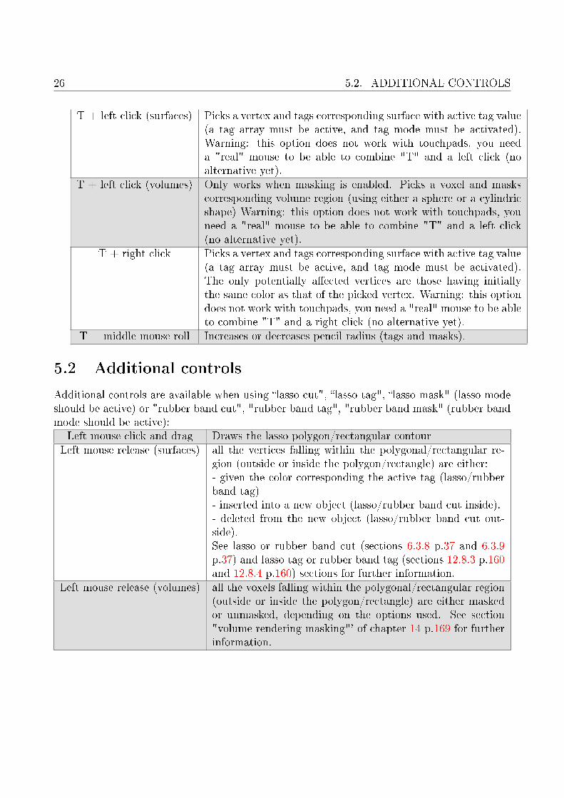
T + left click (surfaces) Picks a vertex and tags corresponding surface with active tag value(a tag array must be active, and tag mode must be activated).Warning: this option does not work with touchpads, you needa "real" mouse to be able to combine "T" and a left click (noalternative yet).
T + left click (volumes) Only works when masking is enabled. Picks a voxel and maskscorresponding volume region (using either a sphere or a cylindricshape) Warning: this option does not work with touchpads, youneed a "real" mouse to be able to combine "T" and a left click(no alternative yet).
T + right click Picks a vertex and tags corresponding surface with active tag value(a tag array must be active, and tag mode must be activated).The only potentially a�ected vertices are those having initiallythe same color as that of the picked vertex. Warning: this optiondoes not work with touchpads, you need a "real" mouse to be ableto combine "T" and a right click (no alternative yet).
T + middle mouse roll Increases or decreases pencil radius (tags and masks).
5.2 Additional controls
Additional controls are available when using �lasso cut", �lasso tag", �lasso mask" (lasso modeshould be active) or "rubber band cut", "rubber band tag", "rubber band mask" (rubber bandmode should be active):
Left mouse click and drag Draws the lasso polygon/rectangular contourLeft mouse release (surfaces) all the vertices falling within the polygonal/rectangular re-
gion (outside or inside the polygon/rectangle) are either:- given the color corresponding the active tag (lasso/rubberband tag)- inserted into a new object (lasso/rubber band cut inside).- deleted from the new object (lasso/rubber band cut out-side).See lasso or rubber band cut (sections 6.3.8 p.37 and 6.3.9p.37) and lasso tag or rubber band tag (sections 12.8.3 p.160and 12.8.4 p.160) sections for further information.
Left mouse release (volumes) all the voxels falling within the polygonal/rectangular region(outside or inside the polygon/rectangle) are either maskedor unmasked, depending on the options used. See section"volume rendering masking"' of chapter 14 p.169 for furtherinformation.

Chapter 6
Main window controls
Contents6.1 Camera controls . . . . . . . . . . . . . . . . . . . . . . . . . . . . . . 28
6.1.1 Camera rotation center . . . . . . . . . . . . . . . . . . . . . . . . . . 28
6.1.2 Orthographic or perspective camera projection . . . . . . . . . . . . . 28
6.1.3 Camera orientation . . . . . . . . . . . . . . . . . . . . . . . . . . . . . 28
6.1.4 Screenshot . . . . . . . . . . . . . . . . . . . . . . . . . . . . . . . . . . 29
6.1.5 Camera rotation around �z" viewing axis . . . . . . . . . . . . . . . . . 29
6.1.6 Clipping plane slider . . . . . . . . . . . . . . . . . . . . . . . . . . . . 31
6.1.7 Zoom . . . . . . . . . . . . . . . . . . . . . . . . . . . . . . . . . . . . 31
6.2 Display controls . . . . . . . . . . . . . . . . . . . . . . . . . . . . . . 31
6.2.1 Grid . . . . . . . . . . . . . . . . . . . . . . . . . . . . . . . . . . . . . 31
6.2.2 Coordinate system orientation helper . . . . . . . . . . . . . . . . . . . 32
6.2.3 Anaglyph . . . . . . . . . . . . . . . . . . . . . . . . . . . . . . . . . . 32
6.2.4 Clipping plane . . . . . . . . . . . . . . . . . . . . . . . . . . . . . . . 33
6.2.5 Backface culling . . . . . . . . . . . . . . . . . . . . . . . . . . . . . . 33
6.2.6 Surface 3D representation controls . . . . . . . . . . . . . . . . . . . . 34
6.3 Object controls . . . . . . . . . . . . . . . . . . . . . . . . . . . . . . . 34
6.3.1 Delete selected objects . . . . . . . . . . . . . . . . . . . . . . . . . . . 34
6.3.2 Create landmark at X,Y,Z . . . . . . . . . . . . . . . . . . . . . . . . . 36
6.3.3 Decrease / Increase landmark number . . . . . . . . . . . . . . . . . . 36
6.3.4 Edit �rst selected surface . . . . . . . . . . . . . . . . . . . . . . . . . 36
6.3.5 Edit �rst selected volume . . . . . . . . . . . . . . . . . . . . . . . . . 36
27
28 6.1. CAMERA CONTROLS
6.3.6 Edit �rst selected landmark . . . . . . . . . . . . . . . . . . . . . . . . 36
6.3.7 Edit �rst selected �ag . . . . . . . . . . . . . . . . . . . . . . . . . . . 37
6.3.8 Lasso cut selected surfaces . . . . . . . . . . . . . . . . . . . . . . . . . 37
6.3.9 Rubber band cut selected surfaces . . . . . . . . . . . . . . . . . . . . 37
6.3.10 object rotation and translation sliders . . . . . . . . . . . . . . . . . . 37
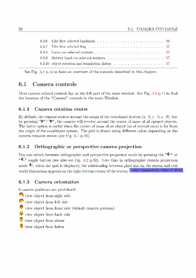
See Fig. 3.1 p.14 to have an overview of the controls described in this chapter.
6.1 Camera controls
Most camera related controls lay on the left part of the main window. See Fig. 3.1 p.14 to �ndthe location of the "Camera" controls in the main Window.
6.1.1 Camera rotation center
By default, the camera rotates around the origin of the coordinate system (x=0, y=0, z=0), butby pressing � "/� ", the camera will revolve around the center of mass of all opened objects.The latter option is useful when the centre of mass of an object (or of several ones) is far fromthe origin of the coordinate system. The grid is drawn using di�erent colors depending on thecamera rotation centre (see Fig. 6.1 p.29).
6.1.2 Orthographic or perspective camera projection
You can switch between orthographic and perspective projection mode by pressing the " " or
" " toggle button (see also see Fig. 6.2 p.30). Note that in orthographic camera projection
mode , when the grid is displayed, the relationship between pixel size on the screen and real
world dimensions appears on the right bottom corner of the screen: .
6.1.3 Camera orientation
6 camera positions are prede�ned :
view object from right side
view object from left side
view object from front side (default camera position)
view object from back side
view object from above
view object from below

CHAPTER 6. MAIN WINDOW CONTROLS 29
Figure 6.1: Grid display color. Left: when the camera revolves around the origin of thecoordinate system (x=0, y=0, z=0), the grid outline is displayed in orange. Right: whenthe camera revolves around the center of mass of all opened objects, the grid has a blueoutline.
6.1.4 Screenshot
Press " " to take a screenshot (.png format). This opens the screenshot dialog (see Fig. 6.3p.30).
6.1.5 Camera rotation around �z" viewing axis
To do so, you may use the slider lying around the center of the leftpanel of the main window.
Figure 6.4:Camera �z"rotation slider

30 6.1. CAMERA CONTROLS
Figure 6.2: Perspective and Orthographic camera projection modes. Skull of Pan panis-
cus. Left: perspective camera projection mode: closer structures appear larger than far-ther structures. Right: orthographic camera projection mode: a uniform relation existsbetween pixel size and real world dimensions, making it possible to place a scale bar.
Figure 6.3: Screenshot dialog. You can de�ne here the multiplication factor in x and y,and decide whether the background should be transparent or opaque.

CHAPTER 6. MAIN WINDOW CONTROLS 31
6.1.6 Clipping plane slider
In some cases, you may need to displace the viewing clipping plane.To do so, use the slider lying centrally in the left panel of the mainwindow. See 6.2.4 p.33 for additional clipping plane functionalities.
Figure 6.5:Camera clippingplane slider
6.1.7 Zoom
There are three main ways to modify the �zoom" in MorphoDig :
• You may use the zoom slider laying in the lower part of theleft panel of the main window.
• You may set manually the display scale (Edit→ Edit size unitand grid spacing, then de�ne the display scale: 100 pixelsin size unit). This option is only available in orthographic
projection mode .
• You may use the middle click mouse roll button (roll thewheel).
Figure 6.6:Zoom slider
6.2 Display controls
The display controls mentioned in this section are situated on the top part of the main window(see Fig. 3.1 p.14).
6.2.1 Grid
Press to show / hide the grid. Default grid size is 1 cm / square. Grid size can be editedmanually (viewing opt. → Grid size). Switching between the 6 camera prede�ned positions
de�ned above ( , , , , and ) will a�ect the plane in which the grid is drawn.

32 6.2. DISPLAY CONTROLS
Figure 6.8: Anaglyph display mode. Left: normal display mode. Right: anaglyphdisplay mode. Cranium of the holotype specimen of Pan paniscus.
6.2.2 Coordinate system orientation helper
Press to show / hide the coordinate system orientation helperlying on the bottom left corner of the main 3D window. By default,the labels are de�ned the following way:+z axis : dorsal side-z axis : ventral side+y axis : left side-y axis : right side+x axis : anterior side-x axis : posterior side.You may edit these labels depending on your preferences (for in-stance, depending on the structure you are working with, you mayneed to set �+y" to �labial", and �-y" to �lateral"). To edit orien-tation labels, click on �Edit → Edit orientation labels."
Figure 6.7:Orientation helper
6.2.3 Anaglyph
Press to activate/deactivate anaglyph 3D rendering. See Fig. 6.8 p.32. You then need to
wear "Red/Blue" glasses to visualize objects in 3D.

CHAPTER 6. MAIN WINDOW CONTROLS 33
Figure 6.9: Clipping plane display mode. Cranium of the type specimen of Pan paniscus.Left: normal display mode. Right: clipping plane display mode "on" : permits to visualizeinner structures.
6.2.4 Clipping plane
The button or permits to adjust / readjust the position of the clipping plane at prede�nedpositions (see for instance Fig. 6.9 p.33):
• : the clipping plane is placed at z = 0 (all objects having a z coordinate along z viewingaxis smaller than 0 are hidden).
• : the clipping plane is replaced at its original value : z= - camera.far / 2. This valuepermits to view objects having positive and negative coordinates along z viewing axis.
6.2.5 Backface culling
Hiding backfaces of a surface is useful in some cases to visualize inner structures of a biological
object (see for instance Fig. 6.10 p.34). The button / permits to visualize/hide backfaces:
• : both sides of a given surface object are rendered.
• : backfaces are hidden (only frontfaces are visible).

34 6.3. OBJECT CONTROLS
Figure 6.10: Backface culling display mode. Petrosal bone of Eulemur mongoz. Left:normal display mode: both frontfaces (lighter) and backfaces (darker) are displayed.Right: backface culling mode activated: only frontfaces are displayed, making it easier tovisualize the bony labyrinth.
6.2.6 Surface 3D representation controls
4 di�erent options exist to draw 3D surfaces :
: point normals display mode (Gouraud shading), see Fig. 6.11-A.
: triangle normals display mode, see Fig. 6.11-B.
: wireframe representation display mode, see Fig. 6.11-C.
point cloud display mode, see Fig. 6.11-D
triangle normales + wireframe display mode, see Fig. 6.11-E
6.3 Object controls
See Fig. 3.1 p.14to see where the "object controls" are situated within MorphoDig's mainwindow. Remind that only selected objects are a�ected by these controls.
6.3.1 Delete selected objects
Clicking on " " deletes all selected objects. This action can be undone/redone.

CHAPTER 6. MAIN WINDOW CONTROLS 35
Figure 6.11: Display modes available for a given surface. Single surface representationof the left bony labyrinth of a Lepilemur dorsalis. A: "Point normales" mode (Gouraudshading). B: "Triangle normales" mode. C: "Wireframe" mode. D: "Point cloud" mode.D: "Triangle normales + wireframe" mode.

36 6.3. OBJECT CONTROLS
Figure 6.12: Create landmark at a given X,Y,Z coordinate.
6.3.2 Create landmark at X,Y,Z
Clicking on " " opens the "Create landmark" window (Fig. 6.12 p.36), in which a newlandmark can be created a speci�ed coordinates. This action can be undone/redone..
6.3.3 Decrease / Increase landmark number
Clicking on will increase (= move down in list, if possible) the landmark number of allselected landmarks. Clicking on will decrease (=move up in list, if possible) the landmarknumber of all selected landmarks. These buttons make it possible to reorder landmarks.
6.3.4 Edit �rst selected surface
Clicking on " " opens the "Edit �rst selected surface" window (see chapter 9, Fig. 9.1 p.91for further details), in which several properties of a given surface object can be edited.
6.3.5 Edit �rst selected volume
Clicking on " " opens the "Edit �rst volume" window (see chapter , Fig. 14.1 p.165 forfurther details), in which several properties of a given volume.
6.3.6 Edit �rst selected landmark
Clicking on " " opens the "Edit �rst selected landmark" window (see Fig. 10.1 p.116 forfurther details).

CHAPTER 6. MAIN WINDOW CONTROLS 37
6.3.7 Edit �rst selected �ag
Clicking on " " opens the "Edit �rst selected �ag" window (see Fig. 10.2 p.116 for furtherdetails), in which several properties of a given �ag can be manually edited.
6.3.8 Lasso cut selected surfaces
You may cut through an input selected surface using this option (see Fig. 6.13 p.38). Once
" " (lasso cut keep inside) or " " (lasso cut keep outside) button has been pressed, themouse cursor changes and you can start drawing the lasso section by dragging the mouse whilethe left button is pressed. When the left button is released, the lasso cut operation starts: anew object is created, which contains all the parts of the selected object laying inside or outsidethe drawn polygon, respectively.
6.3.9 Rubber band cut selected surfaces
You may cut through an input selected surface using this option (see Fig. 6.14 p.39). Once
" " (rubber band cut, keep inside) or " " (rubber band cut, keep outside) button has beenpressed, the mouse cursor changes and you can start drawing a rectangular section by draggingthe mouse while the left button is pressed. When the left button is released, the rubber bandcut operation starts: a new object is created, which contains all the parts of the selected objectlaying inside or outside the drawn rectangle, respectively.
6.3.10 object rotation and translation sliders
As seen earlier, selected objects can be translated and rotated using the mouse left and middlebuttons (in landmark and camera selection modes, you also need to maintain �CTRL" buttonpressed while dragging the mouse to achieve rotation and translation of selected objects).Alternatively, you may also use the following controls to accomplish rotation and translationof selected objects. Rotation is performed around the global center of mass of all currentlyselected objects.
Rotation around and translation along �Z" viewing axis
These controls are extremely useful, as there is no way to achieve rotation round � z � viewingaxis or translation along �z" viewing axis using the mouse.To do so, use the tz and rz sliders (see Fig. 6.15 p.40).

38 6.3. OBJECT CONTROLS
Figure 6.13: A: "Lasso keep outside" button is pressed, then a polygon is drawn over theselected object (grey) by maintaining left mouse button pressed and dragging the mouse.B: Left mouse button has been released: a new surface object is created. C: "Delete" hasbeen pressed : only the newly created object remains. C: "Lasso keep inside" is pressed,then a polygon is drawn over the selected object (grey) by maintaining left mouse buttonpressed and dragging the mouse. E: Left mouse button has been released : a new surfaceobject is created. F: "Delete" has been pressed : only the newly created object remains.

CHAPTER 6. MAIN WINDOW CONTROLS 39
Figure 6.14: A: "Rubber band cut keep inside" button is pressed, then a rectangleis drawn over the selected object (grey) by maintaining left mouse button pressed anddragging the mouse. B: Left mouse button has been released: a new surface object iscreated. C: "Delete" has been pressed : only the newly created object remains. C:"Rubber band cut keep outside" is pressed, then a rectangle is drawn over the selectedobject (grey) by maintaining left mouse button pressed and dragging the mouse. E: Leftmouse button has been released : a new surface object is created. F: "Delete" has beenpressed : only the newly created object remains.

40 6.3. OBJECT CONTROLS
Figure 6.15: A: object and tz slider are in initial position. B: tz slider is moved down:the selected object moves forward. C: tz slider is moved up. The selected object movesbackward. D: object and rz slider are in initial position. E: rz slider is moved down: theselected object rotates around the "roll" axis counter-clockwise. F: rz slider is moved up.The selected object rotates around the "roll" axis clockwise.

CHAPTER 6. MAIN WINDOW CONTROLS 41
Rotation/translation around/along �Y" viewing axis
To do so, use the ty and ry sliders (see Fig. 6.16 p.42).
Rotation/translation around/along �X" viewing axis
To do so, use the ty and ry sliders (see Fig. 6.17 p.43).

42 6.3. OBJECT CONTROLS
Figure 6.16: A: object and ty slider are in initial position. B: ty slider is moved down:the selected object moves downward. C: ty slider is moved up. The selected object movesupward. D: object and ry slider are in initial position. E: ry slider is moved down: theselected object rotates around the "yaw" axis clockwise. F: ry slider is moved up. Theselected object rotates around the "yaw" axis counter-clockwise.
CHAPTER 6. MAIN WINDOW CONTROLS 43
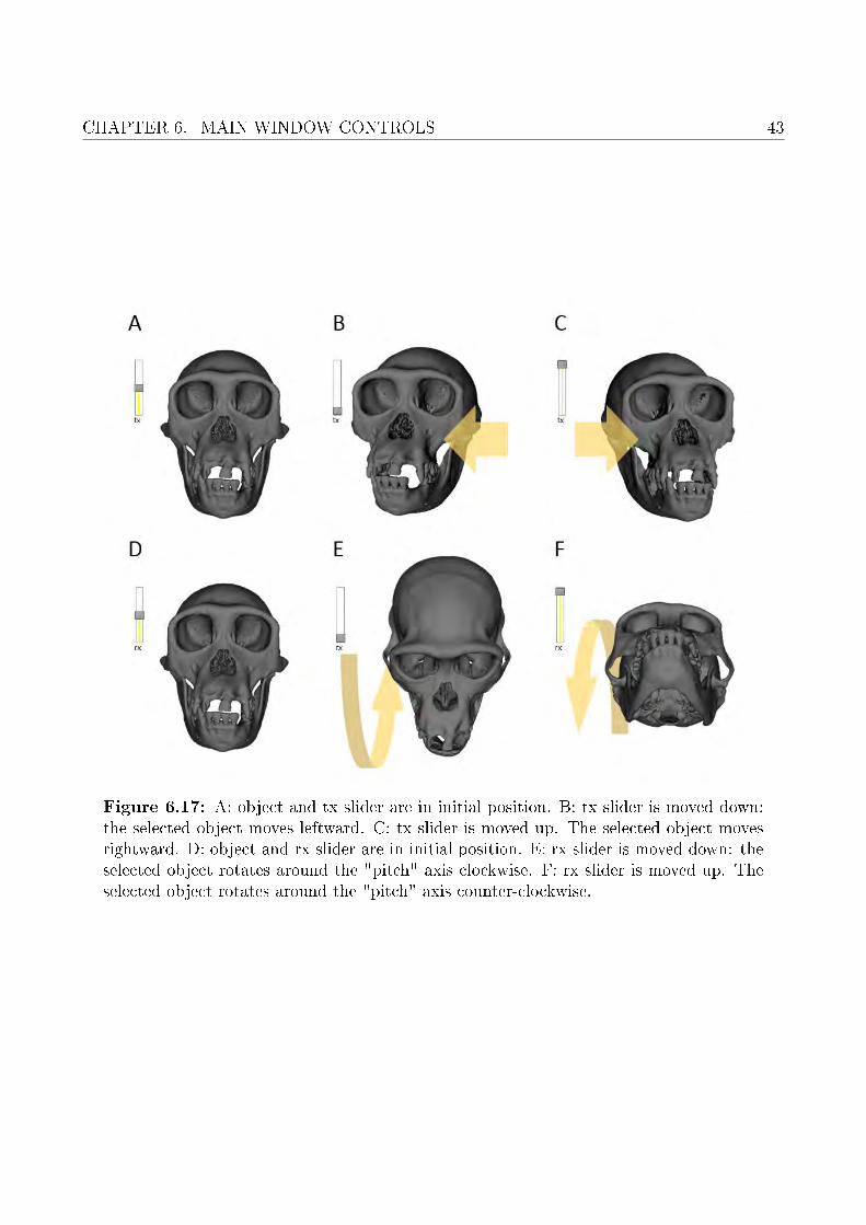
Figure 6.17: A: object and tx slider are in initial position. B: tx slider is moved down:the selected object moves leftward. C: tx slider is moved up. The selected object movesrightward. D: object and rx slider are in initial position. E: rx slider is moved down: theselected object rotates around the "pitch" axis clockwise. F: rx slider is moved up. Theselected object rotates around the "pitch" axis counter-clockwise.

44 6.3. OBJECT CONTROLS
Chapter 7
Menu File
Contents7.1 Project . . . . . . . . . . . . . . . . . . . . . . . . . . . . . . . . . . . . 47
7.1.1 Open project . . . . . . . . . . . . . . . . . . . . . . . . . . . . . . . . 48
7.1.2 Save project . . . . . . . . . . . . . . . . . . . . . . . . . . . . . . . . . 48
7.2 Surface . . . . . . . . . . . . . . . . . . . . . . . . . . . . . . . . . . . . 50
7.2.1 Open surface . . . . . . . . . . . . . . . . . . . . . . . . . . . . . . . . 50
7.2.2 Save surface . . . . . . . . . . . . . . . . . . . . . . . . . . . . . . . . . 51
7.3 Position . . . . . . . . . . . . . . . . . . . . . . . . . . . . . . . . . . . 53
7.3.1 Open position for selected surfaces . . . . . . . . . . . . . . . . . . . . 54
7.3.2 Open transposed position for selected surfaces . . . . . . . . . . . . . . 54
7.3.3 Open position for selected landmarks/�ags . . . . . . . . . . . . . . . . 55
7.3.4 Open transposed position for selected landmarks/�ags . . . . . . . . . 55
7.3.5 Save position for selected surfaces . . . . . . . . . . . . . . . . . . . . . 55
7.3.6 Edit manually position matrix . . . . . . . . . . . . . . . . . . . . . . . 56
7.4 Landmarks . . . . . . . . . . . . . . . . . . . . . . . . . . . . . . . . . 56
7.4.1 Open MorphoDig Landmark/Curve File (STV) . . . . . . . . . . . . . 58
7.4.2 Open Landmarks . . . . . . . . . . . . . . . . . . . . . . . . . . . . . . 58
7.4.3 Open Target Landmarks . . . . . . . . . . . . . . . . . . . . . . . . . . 58
7.4.4 Save MorphoDig Landmark/Curve File (STV) . . . . . . . . . . . . . . 58
7.4.5 Save Landmarks . . . . . . . . . . . . . . . . . . . . . . . . . . . . . . 58
7.4.6 Save Target Landmarks . . . . . . . . . . . . . . . . . . . . . . . . . . 59
7.5 Curves . . . . . . . . . . . . . . . . . . . . . . . . . . . . . . . . . . . . 59
45

46
7.5.1 Open Curve (.CUR) . . . . . . . . . . . . . . . . . . . . . . . . . . . . 61
7.5.2 Open MorphoDig Landmark/Curve �le (.STV) . . . . . . . . . . . . . 61
7.5.3 Open Curve Node Landmarks . . . . . . . . . . . . . . . . . . . . . . . 61
7.5.4 Open Curve Handle Landmarks . . . . . . . . . . . . . . . . . . . . . . 62
7.5.5 Save .CUR �le . . . . . . . . . . . . . . . . . . . . . . . . . . . . . . . 62
7.5.6 Save MorphoDig Landmark/Curve File (STV) . . . . . . . . . . . . . . 62
7.5.7 Save Curve Node Landmarks . . . . . . . . . . . . . . . . . . . . . . . 62
7.5.8 Save Curve Handle Landmarks . . . . . . . . . . . . . . . . . . . . . . 62
7.5.9 Export Curves as Landmark �le . . . . . . . . . . . . . . . . . . . . . . 63
7.5.10 Save curve infos (length per curve segment) . . . . . . . . . . . . . . . 64
7.6 Flags . . . . . . . . . . . . . . . . . . . . . . . . . . . . . . . . . . . . . 64
7.6.1 Load �ags . . . . . . . . . . . . . . . . . . . . . . . . . . . . . . . . . . 64
7.6.2 Save �ags . . . . . . . . . . . . . . . . . . . . . . . . . . . . . . . . . . 64
7.7 Color maps . . . . . . . . . . . . . . . . . . . . . . . . . . . . . . . . . 65
7.7.1 Import color maps (.MAP) . . . . . . . . . . . . . . . . . . . . . . . . 65
7.7.2 Export color maps (.MAP) . . . . . . . . . . . . . . . . . . . . . . . . 66
7.8 Tag maps . . . . . . . . . . . . . . . . . . . . . . . . . . . . . . . . . . 66
7.8.1 Import tag maps (.TGP or .TAG) . . . . . . . . . . . . . . . . . . . . 67
7.8.2 Export tag maps (.TGP or .TAG) . . . . . . . . . . . . . . . . . . . . 68
7.9 Orientation helper labels . . . . . . . . . . . . . . . . . . . . . . . . . 68
7.9.1 Open Orientation labels . . . . . . . . . . . . . . . . . . . . . . . . . . 68
7.9.2 Save Orientation labels . . . . . . . . . . . . . . . . . . . . . . . . . . . 68
7.10 Measurements . . . . . . . . . . . . . . . . . . . . . . . . . . . . . . . 68
7.10.1 Save area, volume, triangle number and vertex number of selectedsurfaces . . . . . . . . . . . . . . . . . . . . . . . . . . . . . . . . . . . 68
7.10.2 Complexity: save normalized shape index, area and volume of selectedsurfaces . . . . . . . . . . . . . . . . . . . . . . . . . . . . . . . . . . . 69
7.10.3 Complexity: save convex hull area ratio and convex hull normalizedshape index of selected surfaces (warning: slow). . . . . . . . . . . . . 70
7.10.4 Save size measurements (max length in xyz direction etc.) of all se-lected surfaces. . . . . . . . . . . . . . . . . . . . . . . . . . . . . . . . 71
7.10.5 Save active scalar infos (mean, median, variance ...) of all selectedsurfaces. . . . . . . . . . . . . . . . . . . . . . . . . . . . . . . . . . . . 71
7.10.6 Save scalar values of �rst selected surface. . . . . . . . . . . . . . . . . 72

CHAPTER 7. MENU FILE 47
7.11 Volume . . . . . . . . . . . . . . . . . . . . . . . . . . . . . . . . . . . . 72
7.11.1 Open MHD/MHA/VTI volume . . . . . . . . . . . . . . . . . . . . . . 72
7.11.2 Open Raw Volume . . . . . . . . . . . . . . . . . . . . . . . . . . . . . 72
7.11.3 Open 3D ti� �le . . . . . . . . . . . . . . . . . . . . . . . . . . . . . . 72
7.11.4 Open stack of 2D ti� �les . . . . . . . . . . . . . . . . . . . . . . . . . 72
7.11.5 Open DICOM 2D stack . . . . . . . . . . . . . . . . . . . . . . . . . . 75
7.11.6 Open BMP image stack . . . . . . . . . . . . . . . . . . . . . . . . . . 75
7.11.7 Open PNG image stack . . . . . . . . . . . . . . . . . . . . . . . . . . 75
7.11.8 Import MHD/MHA/VTI Mask and apply it to �rst selected volume . 76
7.11.9 Save �rst selected volume as .MHD or .MHA �le . . . . . . . . . . . . 76
7.11.10Save �rst selected volume as .VTI . . . . . . . . . . . . . . . . . . . . 76
7.11.11Export mask of �rst selected volume as .MHD or .MHA �le . . . . . . 76
7.1 Project
When working with multiple surface objects, loading surfaces and associated positions one byone becomes fastidious. Besides, after having digitized landmarks, �ags, after having set tagnames and colors, or after having de�ned orientation labels, you may wish to open or save thisinformation along with surface �les. You may open and save series of surface �les and associ-ated position matrices, landmarks, �ags, tag colors and labels and orientation labels using thismenu. �Project" �les (.ntw) �les are organized the following way (see Fig. 7.1 p.48):- Optional: name of orientation label �le (.ori)- Optional: name of tag �le (.tag)- Optional: name of �ag �le (.�g)- Optional: name of landmak �le (.lmk, .ver, .stv or .cur)- Name of surface 1 �le- Name of position 1 �le associated to surface 1- Surface 1 RGB color and transparency- Name of surface 2 �le- Name of position 2 �le associated to surface 2- Surface 2 RGB color and transparency (etc...)- Name of volume 1 �le- Name of position 1 �le associated to volume 1- Name of map 1 �le associated to volume 1- Scalar opacity unit distance, min and max values to plot for volume 1- Name of volume 2 �le- Name of position 2 �le associated to volume 2

48 7.1. PROJECT
Figure 7.1: Example of project .ntw �le containing references to orientation labels, tagslabels and colors, �ags and landmarks �les.
- Name of map 2 �le associated to volume 2- Scalar opacity unit distance, min and max values to plot for volume 2 (etc.)
Surface �les can be of the following types : .stl, .vtk and .ply�.ntw" �les can be constructed manually, providing that the referred surface, volume, map andposition �les exist.
7.1.1 Open project
Loads a .ntw �le
7.1.2 Save project
Behavior: only selected elements (surface objects, landmarks, �ags, volumes...) are saved withinprojects. If at least one opened element has been selected, the Save project window (Fig. 7.2p.49) opens and asks whether :
• orientation labels should be saved along with the project (by default, orientation labelsare not saved, as orientation labels are quite rarely set by users).
• tag legends and colors (tag maps) should by saved. By default, .tag �le are not savedalong with the project, as tag setting is not a common task.
• save surfaces as VTP (VTK XML polydata), VTK polydata, PLY or STL. We advise youto save your surfaces as VTK polydata (.vtp or .vtk). In the contrary case, all scalars,tag arrays and RGB arrays will be lost. Once exception: one RGB array named exactly"RGB" can be saved within PLY �les.
• save volumes as MetaImage Header and Raw volume �les (.mhd and .raw or .zraw),Metaimage volumes (.mha) �les, VTK Images (.vti). Allow compression on/o� (only forMHD and MHA �les).

CHAPTER 7. MENU FILE 49
Figure 7.2: Save project window.

50 7.2. SURFACE
• save position inside .POS �le, or harden the position. We advise you to save position inside.POS �le (when harden transformed, the information regarding the original orientationsof your surfaces will be lost).
Each surface �le will be given the name of the original �le. Each position �le will be givena name which starts with the name of the associated surface and ends with the name of theproject (1 exception: when the project contains only one surface and the project's name is thesame as that of the surface. In that case, .pos �le names are not post�xed with the name ofthe project). In the .ntw �le example shown in Fig. 7.1 p.48, the surface �les are
• �Hippopotamus_amphibius_braincase.vtk"
• �Hippopotamus_amphibius_bulla.vtk"
• �Hippopotamus_amphibius_petrosal.vtk"
• �Hippopotamus_amphibius_sinus.vtk"
and the project name is �exploded.ntw". The advantage of naming position �les that way isyou may construct di�erent .ntw �les with di�erent associated surface �les using a same set ofsurfaces. Requirement : all selected surfaces saved via this option need to have distinct names.Note : When working with �project" �les, if several surface objects have the same name, youmay need at some point to rename some of the object surfaces in order to make sure that all
surface objects have a distinct name. To do so, select one surface, click on : the �Edit �rstselected surface" window appears (See Fig. 9.1 p.91).
7.2 Surface
7.2.1 Open surface
STL, PLY, VTK/VTP polydata and OBJ surfaces can be opened via this menu. MorphoDigdoes not manage textures associated with surface �les. When opening a PLY �le containingRGB colors (for instance a �le painted manually or automatically with �MeshLab", or somelaser scanner surface �les) or a VTK �le containing RGB arrays, these colors are placed insidea (or several) "RGB" array(s).

CHAPTER 7. MENU FILE 51
7.2.2 Save surface
Selected surfaces can be saved into �les. If no surface is selected, the following message appears:
If at least 2 surfaces are selected, the following message shows up:
Save selected surfaces in one single .PLY �le
Options:
• File type: you can save .ply data in binary(little or big endian) or ASCII formats.
• Position : you can keep object original co-ordinate system or save the surface in itscurrent position.
• Normals : you can choose whether youwish to save normals.
• Colors : RGB information associated toeach vertex can be saved. You may decideeither to keep current RGB color array (ifthat array exists). Alternatively, you maydecide not to save the current RGB colorarray (if it exists). Finally, you may pre-fer to save/replace the current RGB colorarray as the current display color.
Figure 7.3: PLY save options window
Note that a "RGB" array (object rendering color, depending on which rendering mode youare using), depending on the chosen options, can be saved inside the .ply �le. This means

52 7.2. SURFACE
that Tag / Scalar / Object solid color can be exported and viewed in other software such asMeshLab.
Save selected surfaces in one single .VTK PolyData (.VTK or .VTP) �le
VTK polydata surface �le format is by far not aswidespread as STL or PLY formats. However,it is extremely useful as it allows to store severalscalar, tag and RGB arrays. Options:
• File type: you can save .VTK data in bi-nary (little endian) or ASCII formats.
• Position : you can keep object original co-ordinate system or save the surface in itscurrent position.
• Arrays: you decided which arrays (scalars,tags, RGB colors) should be saved insidethe VTK polydata �le.
Figure 7.4: VTK save options window

CHAPTER 7. MENU FILE 53
Save selected surfaces in one single .STL �le
Options:
• File type: you can save .stl data in binary(little endian) or ASCII formats.
• Position : you can keep object original co-ordinate system or save the surface in itscurrent position
Figure 7.5: STL save options window
Save selected surfaces in one single .OBJ �le
Options:
• Position : you can keep object original co-ordinate system or save the surface in itscurrent position
Figure 7.6: OBJ save options window
7.3 Position
In MorphoDig, surface position consists in two 4*4 square matrices: the �rst matrix is currentlynot read nor used anymore by MorphoDig, but is kept for compatibility issues with older versionsof MorphoDig and of ISE-MeshTools (MorphoDig is a major redesign of an older software, ISE-MeshTools). This �rst matrix will disappear in a near future. The second matrix is the onethat matters: the position matrix. It contains the rotation and translation information of 3D

54 7.3. POSITION
Figure 7.7: Example of .pos position �le. The �rst 4 lines correspond to the aspectmatrix, and the 4 last lines to the position matrix.
objects (3D surfaces and landmarks). These 2 matrices can be opened and saved in �.pos"format (see Fig. 7.7 p.54).
7.3.1 Open position for selected surfaces
If no surface is selected, the following message appears:
If at least 2 surfaces objects are selected, the same position will be given to them.
7.3.2 Open transposed position for selected surfaces
This option may be useful in the following case:
• Let us suppose that you did modify the position of a given surface and saved its position.
• Then you have saved the surface in its current modi�ed position (= the original positionof the surface is lost).
It may happen that you need to open the surface in its original position. To do so, you mayapply this option (apply transposed position matrix to the modi�ed surface).

CHAPTER 7. MENU FILE 55
7.3.3 Open position for selected landmarks/�ags
If no landmark/�ag is selected, the following message appears:
This options may be useful when you have digitized landmarks/�ags on a given surface in itsoriginal position and orientation. Let us suppose that in a second step, you need to modify theposition/orientation of that surface object and that you save it in a .POS �le. You may thenapply this .POS �le to your set of landmarks/�ags.
7.3.4 Open transposed position for selected landmarks/�ags
If you have digitized landmarks/�ags on a surface with a modi�ed position (let us assume thatthe position of this surface is saved within a .POS �le), by using this option, you can replacethis landmarks/�ags dataset on the surface in its original orientation.
7.3.5 Save position for selected surfaces
Surface aspect and position matrices can be saved in �.pos" format. If no surface is selected,the following message appears:
If at least 2 surfaces selected, the following message shows up:

56 7.4. LANDMARKS
7.3.6 Edit manually position matrix
Clicking on " " opens the "Edit �rst selected surface" window (Fig. 9.1 p.91), in which theposition matrix of a given actor can be modi�ed.
7.4 Landmarks
Landmarks can be set on surfaces by pressing �L" + left mouse click.
Two series of conventional landmarks can be set : �normal" and �target" landmarks. In
the �normal" landmark mode (button active), pressing �L" + left mouse click results in the
creation a �normal" landmark (a light green one). In the �target" landmark mode (buttonactive), pressing �L" + left mouse click will create a �target" landmark (a yellow transparentone).
�Normal" and �target" landmarks can be loaded and saved.Selected landmarks can be reordered using the following buttons. Pressing � " will (try to)increase the number of all selected landmarks, while pressing � � "" will (try to) decrease theirnumber, respectively.
MorphoDig can manage three types of landmark �les: �.LMK", �.VER" and �.STV" �les.
• .LMK �les contain a series of lines, each line being constructed the following way (seeFig. 7.8 p.57): landmark name (without space or tab character), landmark coordinates.Note that each landmark name does not need to be of the form �landmark"+landmarknumber. Meanwhile, the name should not hold space or tab characters.
• .VER �les contain a series of lines, each line being constructed the following way (seeFig. 7.9 p.57): landmark name (without space or tab character), landmark coordinates,landmark orientation.
• STV �les may contain one or two series of line. The �rst line contains two integers, the�rst being the type of landmark (0 for �normal" or 1 for �target"), the second being thenumber of lines of landmarks of this type which are expected to follow, constructed thefollowing way: landmark name (without space or tab character), landmark coordinates,landmark orientation. An example of .STV �le containing both �normal" and �target"landmarks is given in Fig. 7.10 p.57. Note that the number of �normal" and �target"landmarks saved within a .STV �le can di�er.

CHAPTER 7. MENU FILE 57
Figure 7.8: Example of .LMK �le
Figure 7.9: Example of .VER �le
Figure 7.10: Example of .STV �le. We advise you to use this �le format.

58 7.4. LANDMARKS
Figure 7.11: Save STV window.
7.4.1 Open MorphoDig Landmark/Curve File (STV)
STV �le contain lists of "normal", "target" landmarks (but may also contain lists of "curvenode" and "curve handle" landmarks).
7.4.2 Open Landmarks
Landmarks (.VER or .LMK) opened using this option will be put in the �normal" landmarklist (light green landmarks)
7.4.3 Open Target Landmarks
Landmarks opened using this option will be put in the �target" landmark list (yellow transparentlandmarks)
7.4.4 Save MorphoDig Landmark/Curve File (STV)
You may decide whether you wish to save all (normal, target, curve node, curve handle) land-marks or only selected ones (see Fig. 7.11 p.58).
7.4.5 Save Landmarks
You may decide whether you wish to save only selected �normal" landmarks or all selected andunselected �normal" landmarks (the yellow transparent ones) in .VER or .LMK format (seeFig. 7.12 p.59). . The �Landmarks" chapter (chapter 10 p.115) and the tutorial �working withlandmarks" contain further information regarding landmark digitization with MorphoDig.

CHAPTER 7. MENU FILE 59
Figure 7.12: Save Landmark Window. Used to save either "Normal", "Target" land-marks (but not both at the same time). This windows is also used to save curve nodes orcurve handles in .LMK and .VER format (but also not both at the same time).
7.4.6 Save Target Landmarks
You may decide whether you wish to save only selected �target" landmarks or all selected andunselected �target" landmarks (the yellow transparent ones) in .VER or .LMK format (seeFig. 7.12 p.59). The �Landmarks" chapter (chapter 10 p.115) and the tutorial �working withlandmarks" contain further information regarding landmark digitization with MorphoDig
7.5 Curves
3D Curves (series of 3D cubic Bezier curves) are constructed in MorphoDig using 2 series oflandmarks : a series of N �curve node" landmarks, and a series of N �curve handle". Curvenodes and handles can be set on surfaces by pressing �L" + left mouse click.
In the �curve nodes" landmark mode (button active), pressing �L" + left mouse clickresults in the creation a �curve node" landmark (a dark green for a curve starting node, and
then light red ones). In this mode (�curve nodes" landmark mode = active), pressing �Shift"+ left mouse click results in the creation a new starting �curve node" landmark; pressing �J"+ left mouse click results in the creation a new milestone �curve node" landmark; pressing �K"+ left mouse click results in the creation a new �curve node" landmark that will be connectedto the preceding starting node to close the curve;
In the �curve handles" landmark mode (button active), pressing �L" + left mouse click
60 7.5. CURVES
will create a �target" landmark (a violet transparent one).Selected curve nodes/handles can be reordered using the following buttons. Pressing � "
will (try to) increase the number of all selected curve nodes/handles, while pressing � � "" will(try to) decrease curve nodes/handles number, respectively.
3D Bezier curves passing through all curve nodes are draw green when no curve node/handlebelonging to the curve segment is selected. Curves are drawn red when at least one curvenode/handle involved in the curve segment is selected. Two di�erent cases are considered:
• Case 1: the numbers of �curve node" and �curve handle" landmarks di�er. In that case,a curve is a series of lines passing through �curve node" landmarks.
• Case 2: the numbers of �curve node" and �curve handle" landmarks are equal. In thatcase, a curve is a series of cubic Bezier curves passing through �normal" landmarks. Fora given set of 2 �curve node" consecutive landmarks (Ln and Ln+1) and their associated�curve handles" (Hn and Hn+1), a mirror image of Hn+1 relative to Ln+1 (H'n+1) isconstructed. The Bezier curve involving Ln, Ln+1, Hn and Hn+1 starts from Ln, goingtoward Hn, and arrives at Ln+1 coming from the direction of H'n+1.
The explicit form of the curve is :
B(t) = (1− t)3Ln+ 3(1− t)3tHn+ 3(1− t)t2H ′n+ 1 + t3Ln+ 1, t ∈ [0, 1] (7.1)
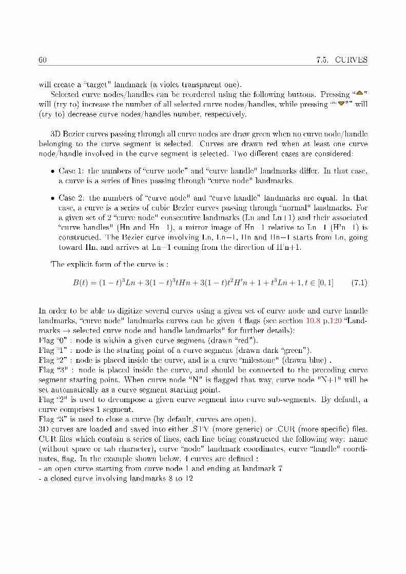
In order to be able to digitize several curves using a given set of curve node and curve handlelandmarks, �curve node" landmarks curves can be given 4 �ags (see section 10.8 p.120 �Land-marks → selected curve node and handle landmarks" for further details):Flag �0" : node is within a given curve segment (drawn �red").Flag �1" : node is the starting point of a curve segment (drawn dark �green").Flag �2" : node is placed inside the curve, and is a curve �milestone" (drawn blue) .Flag �3" : node is placed inside the curve, and should be connected to the preceding curvesegment starting point. When curve node "N" is �agged that way, curve node "N+1" will beset automatically as a curve segment starting point.Flag �2" is used to decompose a given curve segment into curve sub-segments. By default, acurve comprises 1 segment.Flag �3" is used to close a curve (by default, curves are open).3D curves are loaded and saved into either .STV (more generic) or .CUR (more speci�c) �les.CUR �les which contain a series of lines, each line being constructed the following way: name(without space or tab character), curve �node" landmark coordinates, curve �handle" coordi-nates, �ag. In the example shown below, 4 curves are de�ned :- an open curve starting from curve node 1 and ending at landmark 7- a closed curve involving landmarks 8 to 12

CHAPTER 7. MENU FILE 61
Figure 7.13: Example of .CUR �le
- an open curve involving landmarks 13 to 20- a closed curve involving landmarks 21 to 26These four curves contain only one sub-segment (no curve milestone was set within those 4curves). Note that each name does not need to be of the form �CurvePart"+ number. Mean-while, the name should not hold space or tab characters.
7.5.1 Open Curve (.CUR)
This menu allows the user to load a .CUR �le.
7.5.2 Open MorphoDig Landmark/Curve �le (.STV)
This menu allows the user to load a STV �le, as STF �les can contain lists of curve node andcurve handle landmarks (see for instance Fig. 7.10 p.57).
7.5.3 Open Curve Node Landmarks
This menu allows the user place the content of a VER or LMK �le inside the list of curve nodelandmarks.

62 7.5. CURVES
7.5.4 Open Curve Handle Landmarks
This menu allows the user place the content of a VER or LMK �le inside the list of curve handlelandmarks.
7.5.5 Save .CUR �le
This menu allows the user to save current landmarks and curve handles as a .CUR �le. Thisaction is only allowed if the number of �curve node" landmarks and �curve handle" landmarksis the same. If not, the following message appears:
If you are in the process of digitizing curves (and do not have achieved to digitize the samenumber of �normal" and �target" landmarks and wish to save the current state of your work,you may decide to save curve node and target landmarks within a STV �le instead (see nextsection ).
7.5.6 Save MorphoDig Landmark/Curve File (STV)
You may decide whether you wish to save all curve node and curve handle landmarks or onlyselected ones (see Fig. 7.11 p.58). Using this option will also save "normal" and "target"landmark lists.
7.5.7 Save Curve Node Landmarks
Curve node landmarks can be saved inside a LMK or VER �le using this option. You may decidewhether you wish to save only selected �curve node" landmarks or all selected and unselected�curve node" landmarks in .VER or .LMK format (see Fig. 7.12 p.59).
7.5.8 Save Curve Handle Landmarks
Curve handle landmarks can be saved inside a LMK or VER �le using this option. You maydecide whether you wish to save only selected �curve handle" landmarks or all selected andunselected �curve handle" landmarks in .VER or .LMK format (see Fig. 7.12 p.59).

CHAPTER 7. MENU FILE 63
Figure 7.14: Export curves as landmark �le window. Here, 5 curve segments have beendigitized, and the default number of landmarks per segment is 60, but the user has chosento export segments 2 and 4 using 20 equidistant landmarks instead.
7.5.9 Export Curves as Landmark �le
Curves can be transformed in a series of equidistant landmarks using this option. The curvedecimation window appears. Each curve segment is saved as a number of equidistant land-marks.Be aware that there are two ways to de�ne curve segments in MorphoDig :- by setting curve node "starting points" , in order to create independent curve segments (seesection 10.8.2 p.120, and a practical example Fig. 10.9 p. 122)- by setting curve node "milestones", in order to create contiguous curve segments (see section10.8.4 p.120, and a practical example Fig. 10.11 p. 123).You may also decide to save normal and target landmarks information inside the output. Thisis useful when you need to use both type 1 landmarks (normal and target landmarks) andsemi-landmards (3D curves) in Geometric Morphometric analyses.
In the example presented Fig. 7.14 p. 63, 5 segments have been digitized, and the defaultnumber of landmarks per segment is 60, but the user has chosen to export segments 2 and 4using 20 equidistant landmarks instead.

64 7.6. FLAGS
7.5.10 Save curve infos (length per curve segment)
Each curve segment length can be saved as a .txt�le using this option. As stated in the precedingsection, we want to insist on the fact that there aretwo ways to de�ne curve segments in MorphoDig :- by setting curve node "starting points" , in orderto create independent curve segments (see section10.8.2 p.120, and a practical example Fig. 10.9 p.122)- by setting curve node "milestones", in order tocreate contiguous curve segments (see section10.8.4 p.120, and a practical example Fig. 10.11 p.123).
The �Landmarks" chapter (chapter 10 p.115) andthe tutorial �Working with curves" contain furtherimportant information regarding curve digitizationwith MorphoDig.
Figure 7.15: Example of curve info�le
7.6 Flags
Regarding �ags, as stated earlier, one series of ��ag landmarks" can be digitized in MorphoDig
(button ` " should be pressed). To edit �ag label, length and color, select one �ag landmark,
click on " " in order to open the "Edit �rst selected landmark" window (Fig. 10.2 p.116).Pressing ok will update the label, the color and the length associated to the selected �ag, whichin turn will be unselected.
Flags are saved using the .FLG �le format, which consists of n pairs of lines constructed thefollowing way (Fig. 7.16 p.65):line 2*n: Flag nameline 2*n+1: Flag coordinates, �ag orientation, �ag length and color.
7.6.1 Load �ags
Select a .FLG �le using this menu
7.6.2 Save �ags
This option saves the current �ag landmarks into a .FLG �le, regardless their selection status.

CHAPTER 7. MENU FILE 65
Figure 7.16: Example of .FLG �le
7.7 Color maps
- Color maps are used to visualize scalar arrays (=arrays of numbers associated to each vertex)
and can be edited interactively by clicking on , which opens the "Scalar rendering options"window (see chapter �Scalars" (chapter 11 p.127) and the tutorial �Working with scalars" forfurther information).
- Scalars become visible when the array display mode button is pressed ( ), and a scalar array
is selected (ex: ).Two default color maps exist in MorphoDig, which can be edited, but not deleted : the "Rain-bow" the "Black-Red-White" color maps. Any number of additional color maps can be addedto the list of existing color maps, and are referred to as "custom color maps".
An example of color map (.MAP) �le and how it translates into an actual color/opacitymap is shown Fig. 7.17 p.66):
7.7.1 Import color maps (.MAP)
Imports one or several color maps included inside a .MAP �le.

66 7.8. TAG MAPS
Figure 7.17: A. Example of .MAP �le containing one single colormap named "Rainbow",and having 5 color and 4 opacity control points. B. Translation of this colormap insideMorphoDig.
7.7.2 Export color maps (.MAP)
This option opens the Export color maps window,in which the active color map, all color maps (the 2default color maps + all custom color maps), or allcustom color maps can be saved inside a .MAP �le.
Figure 7.18: Export color mapswindow.
7.8 Tag maps
- Tag colors and names (=tag maps) can be edited interactively by clicking on , which opensthe Tags window (see the chapter �Tags" (chapter 12 p.151) and the tutorial �Working withtags" for further information).
- Tags become visible when the array display mode button is pressed ( ), and a tag array is
selected (ex: ).Tag maps consist mostly of a series of combination of a tag name and an associated color.
Any number of tag name + color can be de�ned (25 di�erent names+colors by default, butthis number can be interactively increased/decreased).

CHAPTER 7. MENU FILE 67
By default, MorphoDig contains one Tag maps named "TagMap", which can not be deleted,but can be edited as needed. Other tag maps can be added manually to tag map list, and arereferred to as "custom tag maps".
Tag map �les come in two formats : .TAG and .TGP.
TAG format consists of N pairs of lines, can storeone single tag map, and is constructed the followingway: line 2*n: Tag nameline 2*n+1: Tag color and transparency
Figure 7.19: Example of .TAG �le
TGP format di�ers from TAG in that it can storeseveral tag maps and gives a name to each tag map.An example of TGP �le containing 2 tag maps isshown aside.line 2*n: Tag nameline 2*n+1: Tag color and transparency
Figure 7.20: Example of .TGP �lecontaining two tag maps. The �rstcontains 3 entries, the second 4 en-tries.
7.8.1 Import tag maps (.TGP or .TAG)
Imports one tag map (.TAG or .TGP �le) or several tag maps (.TGP �le). Then open the tag
window (click on ) : Tag labels, colors and transparencies should have been updated. In the"Tags window", you can switch between di�erent tag maps with the combo box "Choose tagmap".

68 7.9. ORIENTATION HELPER LABELS
7.8.2 Export tag maps (.TGP or .TAG)
This option opens the Export tag maps window, inwhich the active tag map, all tag maps (= defaulttag map + all custom tag maps), or all custom tagmaps can be saved inside either a .TAG �le (if onlyone tag map should be saved) or inside a .TGP �le(one or several tag maps).
Figure 7.21: Export tag maps win-dow.
7.9 Orientation helper labels
The coordinate system orientation helper labels can be saved into �.ORI" �les, which are .txt�les containing 6 lines, 1 for each axis.
7.9.1 Open Orientation labels
Select a .ORI �le using this menu. Then open the orientation labels window window (Edit→EditOrientation labels) : the 6 orientation labels should have been updated.
7.9.2 Save Orientation labels
This option saves the current state of orientation labels in a .ORI �le.
7.10 Measurements
7.10.1 Save area, volume, triangle number and vertex number of se-lected surfaces
This option opens the "Surfaces: save infos" dialog (see Fig. 7.22 69), and saves within a .txt�le, and for all selected surfaces, surface area, volume, triangle number and vertex number.If the "Save Area/Volume for each Tagged region?" option is checked and if the selected tagarray exists for the involved surfaces, then for each tagged region, surace area, the volume ,triangle numer and vertex number is also computed. Note that as tags are currently performedon vertices and not on triangles, there are di�erent possibilities to consider whether a given
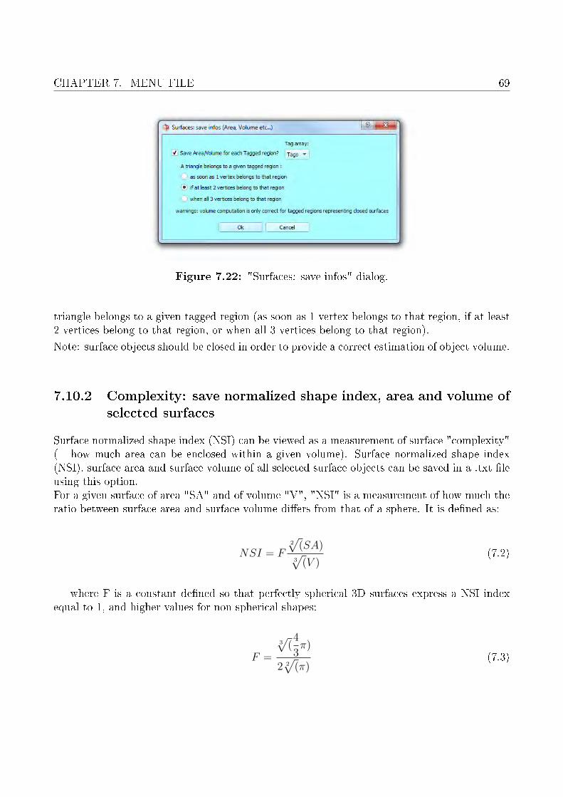
CHAPTER 7. MENU FILE 69
Figure 7.22: "Surfaces: save infos" dialog.
triangle belongs to a given tagged region (as soon as 1 vertex belongs to that region, if at least2 vertices belong to that region, or when all 3 vertices belong to that region).
Note: surface objects should be closed in order to provide a correct estimation of object volume.
7.10.2 Complexity: save normalized shape index, area and volume ofselected surfaces
Surface normalized shape index (NSI) can be viewed as a measurement of surface "complexity"(= how much area can be enclosed within a given volume). Surface normalized shape index(NSI), surface area and surface volume of all selected surface objects can be saved in a .txt �leusing this option.For a given surface of area "SA" and of volume "V", "NSI" is a measurement of how much theratio between surface area and surface volume di�ers from that of a sphere. It is de�ned as:
NSI = F2√
(SA)3√
(V )(7.2)
where F is a constant de�ned so that perfectly spherical 3D surfaces express a NSI indexequal to 1, and higher values for non spherical shapes:
F =
3√
(4
3π)
2 2√
(π)(7.3)

70 7.10. MEASUREMENTS
7.10.3 Complexity: save convex hull area ratio and convex hull nor-malized shape index of selected surfaces (warning: slow).
Surface normalized shape index (NSI, see preceding section) may not o�er a good estimate of"global shape complexity" of surfaces, especially when surfaces' shape di�er very much fromthat of a sphere (very �at objects). Other metrics, such as Convex hull area ratio (ChAR), orconvex hull normalized shape index (ChNSI), may be better proxies for a global measurementsof shape complexity for whole surfaces (= how much area can be enclosed within a given vol-ume). ChAR, ChNSI and surface area, surface volume, convex hull, convex hull volume andsurface normalized shape index (NSI: de�ned in the preceding section) of all selected surfaceobjects can be saved in a .txt �le using this option.
ChAR
For a given surface of area "SA", ChAR is the ratio between "SA" and the surface area of theconvex hull of that same surface (ChSA). Its aim is to compare the surface area of a surfacewith that of that of a "wrapping bag" that would enclose that surface. It is de�ned as:
ChAR =SA
ChSA(7.4)
Perfectly spherical 3D surfaces express a ChSA index equal to 1 while, while hihly foldedstructures (such as turbinates) usually express values higher than 1. Shapes spread in spaceand containing a lot of holes may express ChSA values smaller than 1.
ChNSI
For a given surface of area "SA" and of volume "V", "ChNSI" measures how much surface area"SA" can be enclosed within the volume of the convex hull ("ChV") computed for that samesurface It is de�ned as:
ChNSI = F2√
(SA)3√
(ChV )(7.5)
where F is a constant de�ned so that perfectly spherical 3D surfaces express a ChNSI indexequal to 1 :
F =
3√
(4
3π)
2 2√
(π)(7.6)
Perfectly spherical 3D surfaces express a ChNSI index equal to 1. Hihly folded structures(such as turbinates) usually express ChNSI values higher than 1. Shapes spread in space andcontaining a lot of holes may express ChSA values smaller than 1.

CHAPTER 7. MENU FILE 71
7.10.4 Save size measurements (max length in xyz direction etc.) ofall selected surfaces.
Depending on your biological scienti�c question, you may need di�erent measurements of the"size" of your structure of interes. This menu provides di�erent "size metrics" for 3D surfaceswhich can be relevant.
Bounding box length
Bounding box length gives an idea of the maximal length of a 3D surface. However, this metricsdepends on the orientation of the surface, so be careful when using it.
Mean and maximal distances to centroid
For a given surface containing N vertices, the centroid is de�ned as the average x,y,z coordinatesof all N vertices. The mean distance of all N vertices to the centroid, and the maximal distancefor all N vertices to the centroid give information regarding the expansion in 3D space of yourstructure.
PC1, PC2, PC3 length and average of PC1, PC2, PC3
A better alternative to the bounding box length metrics is as follows: for a given surface,MorphoDig computes a Principal Component Analysis (PCA) of all 3D vertex coordinates.Then all vertices are projected on Principal component 1 (PC1), on PC2 and on PC3. Thedi�erence between the maximal projection scores and minimal projection scores on a given PCgive the length of your structure of interest along that axis. PC1 length is a measurement ofthe maximal length of your structure. PC2 and PC3 lengths are measurements of the maximalwidth and height of your structure. PC1, PC2 and PC3 length do not depend on 3D surfaceorientation and are in that sense much reliable metrics than bounding box length.
7.10.5 Save active scalar infos (mean, median, variance ...) of allselected surfaces.
In order to use this option, the array display mode button must be pressed ( ), and a scalar
array must also be selected selected (ex: ).This option opens the "Scalars: save infos" dialog (see Fig. 7.23 72), and saves within a .txt�le, and for all selected surfaces, the mean, the median, and the variance of the selected scalar.If the "Include scalar infos for each Tagged region" option is checked and if a the selected tagarray exists for the involved surfaces, then for each tagged region, the mean, the median andthe variance of the currently active scalar is also computed.

72 7.11. VOLUME
Figure 7.23: "Scalars: save infos" dialog.
7.10.6 Save scalar values of �rst selected surface.
This option saves within a .txt �le, and ONLY for the �rst selected surface containing N vertices,all scalar values for all vertices. Ex: if a given surface contains 3 scalars (ex: thickness,curvature, complexity), the .txt �le will contain the values of the 3 scalar arrays for all Nvertices.
7.11 Volume
7.11.1 Open MHD/MHA/VTI volume
Meta-image volume �les (.mhd and .mha) �les as well as vtk volume �les (.vti) can be openedusing this format. Meta-image volume �les are very convenient as they can be easily producedwith Fiji software. Voxel size is embedded within this format.
7.11.2 Open Raw Volume
This option opens the "Open raw volume" Dialog (see Fig. 7.24 p.73).
7.11.3 Open 3D ti� �le
This option opens the "Open 3D Ti� �le or 2D Ti� /BMP/PNG stack " dialog (see Fig. 7.25p.74). Data type and dimensions are automatically detected, but you have to �ll index orderand voxel size.
7.11.4 Open stack of 2D ti� �les
Once a number of .ti� �les has been selected, the "Open 3D Ti� �le or 2D Ti� stack " dialog(see Fig. 7.25 p.74) will also be opened. Data type and dimensions are automatically detected,

CHAPTER 7. MENU FILE 73
Figure 7.24: Open raw volume dialog. In order to open a raw volume, information isrequired. 1) Data type (8 bits, 16 bits signed or unsigned, 32 bits or 64 bits). 2) Datadimensions in X, Y and Z. 3) Header Size. 4) Given data type, data dimensions andheader size, requested size in bytes must be equal to �lesize. 5) Data endianess: little orbig endian. 6) Index order: slices either are back-to-front or front-to-back ordered. MostCT datasets are back-to-front ordered: the �rst image image is furthest from the viewer,and subsequent images move towards the viewer. If you do not choose the right option, amirror image of your volume will appear on the screen (which can be corrected later on).7) voxel size in x, y and z dimensions (most ofen expressed in mm)

74 7.11. VOLUME
Figure 7.25: Open 3D Ti� �le or 2D Ti�/BMP/PNG stack dialog 1) Index order: sliceseither are back-to-front or front-to-back ordered. Most CT datasets are back-to-frontordered: the �rst image image is furthest from the viewer, and subsequent images movetowards the viewer. If you do not choose the right option, a mirror image of your volumewill appear on the screen (which can be corrected later on). 2) voxel size in x, y and zdimensions (most ofen expressed in mm)

CHAPTER 7. MENU FILE 75
Figure 7.26: Open dicom stack. Index order: slices either are back-to-front or front-to-back ordered. Most CT datasets are back-to-front ordered: the �rst image image isfurthest from the viewer, and subsequent images move towards the viewer. If you do notchoose the right option, a mirror image of your volume will appear on the screen (whichcan be corrected later on).
but you have to �ll index order and voxel size.
7.11.5 Open DICOM 2D stack
Once a number of .dcm or .ima �les has been selected, the "Open 3D Ti� �le or 2D Ti� stack" dialog (see Fig. 7.26 p.75) will also be opened. Data type, data dimensions and voxel sizeare automatically detected, but you have to �ll index order.
7.11.6 Open BMP image stack
Once a number of 8bit .bmp �les has been selected, the "Open 3D Ti� �le or 2D Ti�/BMP/PNGstack " dialog (see Fig. 7.25 p.74) will also be opened. Data type and dimensions are automat-ically detected, but you have to �ll index order and voxel size. Warning: RGB (24 bits) bmp�les can not currently be read.
7.11.7 Open PNG image stack
Once a number of 8bit .png �les has been selected, the "Open 3D Ti� �le or 2D Ti�/BMP/PNGstack " dialog (see Fig. 7.25 p.74) will also be opened. Data type and dimensions are automat-

76 7.11. VOLUME
Figure 7.27: Save volume as MHD/MHA.
ically detected, but you have to �ll index order and voxel size. Warning: RGB (24 bits) png�les can not currently be read.
7.11.8 Import MHD/MHA/VTI Mask and apply it to �rst selectedvolume
A volume must be selected in order to use this option. This option allows to load a mask �leand will use it to mask voxels if the dimensions of the mask �le match those of the selectedvolume and if the mask �le is of unsigned char (8 bits) type.
7.11.9 Save �rst selected volume as .MHD or .MHA �le
A volume must be selected in order to use this option. This menu opens the "Save MHD/MHA"dialog (see Fig. 7.27 p.76). MHD/MHA �les can be compressed.
7.11.10 Save �rst selected volume as .VTI
A volume must be selected in order to use this option. This menu opens the "Save VTI" dialog(see Fig. 7.28 p.77). VTI �les can be compressed using di�erent methods, and can be savedeither using a little endian or big endian byte order.
7.11.11 Export mask of �rst selected volume as .MHD or .MHA �le
A volume must be selected in order to use this option. This option allows to export a mask �le(in unsigned char 8bit MHD or MHA format).
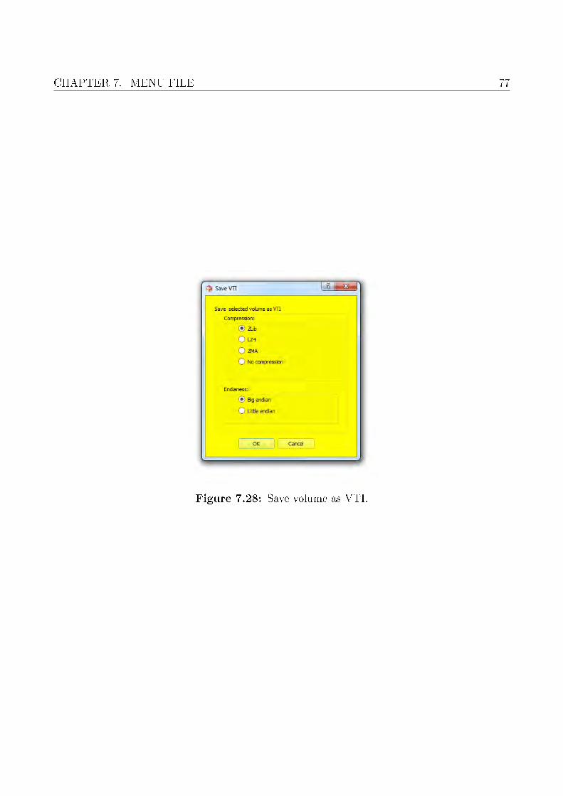
CHAPTER 7. MENU FILE 77
Figure 7.28: Save volume as VTI.

78 7.11. VOLUME

Chapter 8
Menu Edit
Contents8.1 Edit color and lighting options . . . . . . . . . . . . . . . . . . . . . 79
8.2 Edit size unit, grid spacing and scale . . . . . . . . . . . . . . . . . . 80
8.2.1 Size unit . . . . . . . . . . . . . . . . . . . . . . . . . . . . . . . . . . . 80
8.2.2 Grid spacing . . . . . . . . . . . . . . . . . . . . . . . . . . . . . . . . 80
8.2.3 Scale (only valid in orthographic projection mode) . . . . . . . . . . . 82
8.3 Landmark and �ag rendering options . . . . . . . . . . . . . . . . . 82
8.3.1 Landmarks rendering . . . . . . . . . . . . . . . . . . . . . . . . . . . . 82
8.3.2 Flags settings . . . . . . . . . . . . . . . . . . . . . . . . . . . . . . . . 83
8.4 Edit orientation labels . . . . . . . . . . . . . . . . . . . . . . . . . . . 83
8.5 Edit camera options . . . . . . . . . . . . . . . . . . . . . . . . . . . . 86
8.6 Volume options . . . . . . . . . . . . . . . . . . . . . . . . . . . . . . . 86
8.7 Renderer options . . . . . . . . . . . . . . . . . . . . . . . . . . . . . . 86
8.1 Edit color and lighting options
The color and lighting options windows (Fig. 8.1 p.80) makes it possible to edit the defaultsolid color of newly opened surfaces, the background color of the upper part of the 3D window,and the background color of the lower part of the 3D window. The ambient, di�use specularand specular power light settings can be set here as well. Four default presets combinations ofambient, di�use specular lighting and power are available. Default color and light options canbe reinitialized by pressing on the "Reinitialize" button. See Fig. 8.2 p.81 for an example ofthe impact of ambient, di�use and specular light settings on rendering.
79
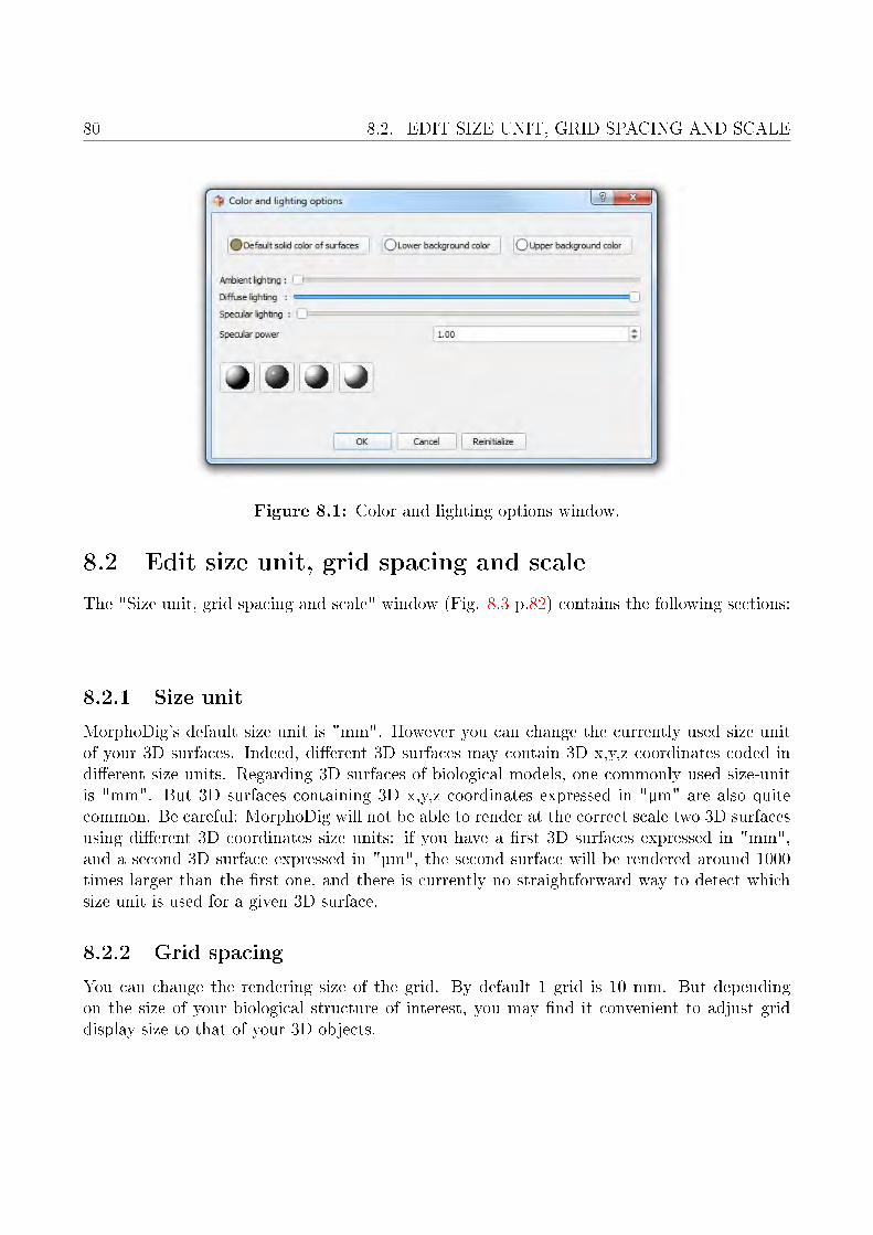
80 8.2. EDIT SIZE UNIT, GRID SPACING AND SCALE
Figure 8.1: Color and lighting options window.
8.2 Edit size unit, grid spacing and scale
The "Size unit, grid spacing and scale" window (Fig. 8.3 p.82) contains the following sections:
8.2.1 Size unit
MorphoDig's default size unit is "mm". However you can change the currently used size unitof your 3D surfaces. Indeed, di�erent 3D surfaces may contain 3D x,y,z coordinates coded indi�erent size units. Regarding 3D surfaces of biological models, one commonly used size-unitis "mm". But 3D surfaces containing 3D x,y,z coordinates expressed in "µm" are also quitecommon. Be careful: MorphoDig will not be able to render at the correct scale two 3D surfacesusing di�erent 3D coordinates size units: if you have a �rst 3D surfaces expressed in "mm",and a second 3D surface expressed in "µm", the second surface will be rendered around 1000times larger than the �rst one, and there is currently no straightforward way to detect whichsize unit is used for a given 3D surface.
8.2.2 Grid spacing
You can change the rendering size of the grid. By default 1 grid is 10 mm. But dependingon the size of your biological structure of interest, you may �nd it convenient to adjust griddisplay size to that of your 3D objects.

CHAPTER 8. MENU EDIT 81
Figure 8.2: Di�erent lighting parameters and resulting rendering of the 3D model ofa left inner ear of Galago moholi. Top line: modi�cation of ambient lighting. Middleline: modi�cation of di�use lighting. Bottom line: modi�cation of specular lighting.

82 8.3. LANDMARK AND FLAG RENDERING OPTIONS
Figure 8.3: Size unit, grid spacing and scale window.
8.2.3 Scale (only valid in orthographic projection mode)
As stated earlier, you can switch between orthographic and perspective projection mode by
pressing the " " or " " toggle button. In this section, you can adjust the display scale(=zoom) in order that 100 pixels on the screen translate into a desired number of size unitsin real world. This option is extremely useful to construct scale bars on scienti�c illustrationsusing software such as Gimp of Photoshop. For instance, if you set the display scale in order tohave 100 pixels = 1 mm and then make a screenshot of your 3D objects in MorphoDig, if youwant to place a scale bar of 5mm, you will simply have to create and draw a 500 pixel-widerectangle over it.
8.3 Landmark and �ag rendering options
The landmark and �ag options window (see Fig. 8.4 p.83) contains the following sections:
8.3.1 Landmarks rendering
�Normal", �Target", �Curve node" and �Curve handle" landmarks can be drawn as spheres or asarrows (composed of a stick and a sphere). Landmark display size can be chosen to be adjustedautomatically (default behaviour) and furthermore adjusted using an adjustment scale factor.
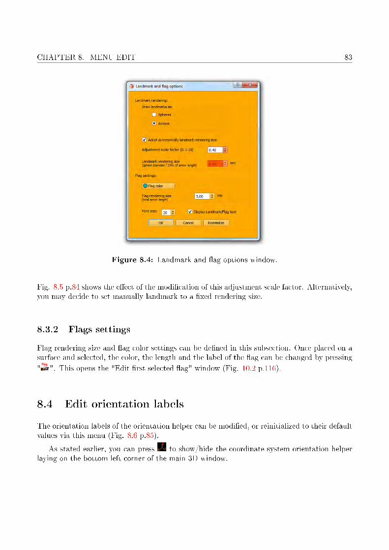
CHAPTER 8. MENU EDIT 83
Figure 8.4: Landmark and �ag options window.
Fig. 8.5 p.84 shows the e�ect of the modi�cation of this adjustment scale factor. Alternatively,you may decide to set manually landmark to a �xed rendering size.
8.3.2 Flags settings
Flag rendering size and �ag color settings can be de�ned in this subsection. Once placed on asurface and selected, the color, the length and the label of the �ag can be changed by pressing
" ". This opens the "Edit �rst selected �ag" window (Fig. 10.2 p.116).
8.4 Edit orientation labels
The orientation labels of the orientation helper can be modi�ed, or reinitialized to their defaultvalues via this menu (Fig. 8.6 p.85).
As stated earlier, you can press to show/hide the coordinate system orientation helperlaying on the bottom left corner of the main 3D window.

84 8.4. EDIT ORIENTATION LABELS
Figure 8.5: Example of the e�ect of di�erent rendering options for the same set oflandmarks (specimen: cranium and mandible of the type specimen of Pan paniscus). A:Landmarks are drawn as spheres, rendering size is adjusted automatically, adjustmentfactor = 1. B: Landmarks are drawn as arrows, rendering size is adjusted automatically,adjustment factor = 1. C: Landmarks are drawn as spheres, rendering size is adjustedautomatically, adjustment factor=0.5. D: Landmarks are drawn as arrows, rendering sizeis adjusted automatically, adjustment factor=0.5.

CHAPTER 8. MENU EDIT 85
Figure 8.6: Edit orientation labels window.
Figure 8.7: Edit camera options window.

86 8.5. EDIT CAMERA OPTIONS
Figure 8.8: Volume options window.
8.5 Edit camera options
The orientation and the position of the camera can be edited, saved, and imported in this section(Fig. 8.7 p.85). This can be useful when constructing a �gure for a scienti�c publication, whenyou want to retrieve the exact position a screenshot was taken.
8.6 Volume options
The default behavior when opening 3D volume data can be set in this section. You may chooseto display directly a volume rendering representation of any opened volume (default behavior),or an XY, XZ or YZ slice instead (Fig. 8.8 p.86). Also, depending on their size, volumerendering representation of 3D data may cause your graphics card to crash. MorphoDig usesthe following strategy : when volumetric dataset volumes contain more than a given numberof voxels, referred to as " out of core threshold" value, MorphoDig automatically computes adownsized representation that will displayed on the screen using volume rendering. You maydecide to adjust the "out of core threshold" depending on your graphics card.
8.7 Renderer options
Transparency rendering of large surface and volumetric dataset is not something straightfor-ward. VTK uses a method called "depth peeling", which uses 2 parameters which allows toadjust the trade-o� between rendering quality and rendering �uidity. In this window, (Fig. 8.9

CHAPTER 8. MENU EDIT 87
Figure 8.9: Renderer options window.
p.87), you may decide to adjust the maximum number of passes allowed by the depth peelingmethod algorithm and the occlusion ratio parameter. An example of the importance of theseparameters is given Fig. 8.10 p.88

88 8.7. RENDERER OPTIONS
Figure 8.10: Transparent rendering of a cranium of Choeropsis liberiensis and internalstructures using di�erent occlusion ratio parameters (image credit: Maëva Orliac). Top-occlusion ratio was set to 0.2 Bottom- occlusion ratio was set to 0.

Chapter 9
Menu Surfaces
Contents9.1 Edit �rst selected surface . . . . . . . . . . . . . . . . . . . . . . . . . 90
9.2 Structure modi�cation . . . . . . . . . . . . . . . . . . . . . . . . . . 90
9.2.1 Smooth each selected surface . . . . . . . . . . . . . . . . . . . . . . . 90
9.2.2 Decimate each selected surface . . . . . . . . . . . . . . . . . . . . . . 93
9.2.3 Densify each selected surface . . . . . . . . . . . . . . . . . . . . . . . 94
9.2.4 Fill holes of each selected surface . . . . . . . . . . . . . . . . . . . . . 95
9.2.5 TPS deformation of each selected surface . . . . . . . . . . . . . . . . 96
9.2.6 Connectivity: separate each selected surface into independent regions . 98
9.2.7 Connectivity: keep largest region for each selected surface . . . . . . . 98
9.2.8 Invert each selected surface . . . . . . . . . . . . . . . . . . . . . . . . 98
9.2.9 Mirror each selected surface along Y plane . . . . . . . . . . . . . . . . 98
9.2.10 Merge selected surfaces into one single surface . . . . . . . . . . . . . . 98
9.3 Wrapping methods . . . . . . . . . . . . . . . . . . . . . . . . . . . . . 101
9.3.1 Create a convex hull for each selected surface . . . . . . . . . . . . . . 101
9.3.2 Shrink and wrap 1 surface over a 2nd surface . . . . . . . . . . . . . . 101
9.4 Boolean operations . . . . . . . . . . . . . . . . . . . . . . . . . . . . 103
9.5 Surface alignment . . . . . . . . . . . . . . . . . . . . . . . . . . . . . 105
9.6 Rendering modi�cation . . . . . . . . . . . . . . . . . . . . . . . . . . 106
9.6.1 Change transparency . . . . . . . . . . . . . . . . . . . . . . . . . . . . 106
9.6.2 Change object solid color . . . . . . . . . . . . . . . . . . . . . . . . . 106
9.7 Create 3D primitives . . . . . . . . . . . . . . . . . . . . . . . . . . . 106
89

90 9.1. EDIT FIRST SELECTED SURFACE
9.7.1 Create cylindric connective struts . . . . . . . . . . . . . . . . . . . . . 107
9.7.2 Create cubic connective struts . . . . . . . . . . . . . . . . . . . . . . . 107
9.7.3 Create icosahedrons / spheres . . . . . . . . . . . . . . . . . . . . . . . 107
9.8 Select small objects . . . . . . . . . . . . . . . . . . . . . . . . . . . . 112
9.9 Select small volumes . . . . . . . . . . . . . . . . . . . . . . . . . . . . 112
In most cases, these function only apply on selected surfaces, so, as a prerequisite, youalmost always need to select surfaces in order to use what is described below.
9.1 Edit �rst selected surface
This menu opens the "Edit �rst selected surface" window (see Fig. 9.1 p.91), in which severalproperties of a given surface object can be edited. This window can also be opened by clicking
on " ". An example of ROI usage can be found Fig. 9.2 p.92.
9.2 Structure modi�cation
9.2.1 Smooth each selected surface
This option uses vtkSmoothPolyDataFilter.Youmay smooth an input selected surface using thisoption (see Fig. 9.4 p.93). A number of itera-tion and a relaxation factor are required.See vtkSmoothPolyDataFilter documentationfor further information regarding this option.
Figure 9.3: Surface smoothing dialog

CHAPTER 9. MENU SURFACES 91
Figure 9.1: Edit �rst selected surface window. 1-Object name : edit the name of the sur-face.Next and preceding object buttons: saves current settings and fetches next/precedingsurface. View/hide object button. 2- Object solid color : modi�es the "solid color" prop-erty of this object. Object translucency : modi�es the translucency this object. Thenumber of points and triangles are available in this section. 3- Object matrix : currentposition/rotation matrix of the object. Reinit matrix: set current matrix to identity. Re-fresh matrix: if edited outside this window, object's matrix is refreshed. Harden transform: apply current position matrix to all the vertices, and reset position matrix to identity.Apply matrix to all selected surfaces : set position/rotation matrix to all other selectedsurfaces. Apply matrix to all surfaces : set position/rotation matrix to all other surfaceseven if they are not selected.4- Enable ROI: must be activated to enable custom clippingplanes. Show/Hide ROI: show ROI to de�ne interactively clipping planes. 5- Existingarrays : list of all scalar/RGB color/tags arrays associated to the vertices of the surfaces.Edit array name : modi�es the name of currently selected array. Duplicate array : dupli-cates currently selected array. Delete array : deletes currently selected array. Ok : savesettings and closes window

92 9.2. STRUCTURE MODIFICATION
Figure 9.2: Example of ROI box usage to digitize landmarks inside surfaces. A- SurfaceROI is enabled, and ROI box is visible. B- Left drag click on the 6 spheres to edit ROIbox bounds. C- Hide ROI box / or unselect surface. D- Now landmarks can be digitizedinside surface.

CHAPTER 9. MENU SURFACES 93
Figure 9.4: Smoothing surfaces. Left: example of original input surface (left inner earof Galago moholi). Right: resulting output surface after 100 iterations using a relaxationfactor of 0.1.
9.2.2 Decimate each selected surface
This option uses vtkDecimatePro andvtkQuadricDecimation �lters. Requirements: to use mesh decimation, a selected surfaceis required (see for instance Fig. 9.6 p.94).See vtkDecimatePro and vtkQuadricDecima-tion documentations for further informationregarding mesh decimation.
Figure 9.5: Decimate window

94 9.2. STRUCTURE MODIFICATION
Figure 9.6: Surface decimation. Left: point cloud rendering of input surface (left innerear of Galago moholi). Right: point cloud rendering of resulting output (vtkQuadricDec-imation �lter, decimation factor: 95%).
9.2.3 Densify each selected surface
This option makes it possible to densify sur-faces using either the vtkDensifyPolyData �l-ter (1 new vertex created at the center ofeach triangle), the vtkLinearSubdivisionFilter(linear subdivision scheme), the vtkLoopSub-divisionFilter (loop subdivision sheme) or thevtkButter�ySubdivisionFilter (butter�y subdi-vision scheme). Requirements : to use meshdensi�cation, a selected surface is required. Anexample of surface densi�cation is presented inFig. 9.8 p.95. Note that mesh densi�cation canbecome extremely slow when using number ofsubdivisions larger than 1. Figure 9.7: Densi�cation dialog

CHAPTER 9. MENU SURFACES 95
Figure 9.8: Surface densi�cation. Left: wireframe rendering of input surface (left innerear of Galago moholi). Right: wireframe rendering of resulting output (method: 1 newvertex at the center of each triangle; number of subdivisions: 1).
9.2.4 Fill holes of each selected surface
This option uses vtkFillHolesFilter. Require-ments : to use mesh hole �lling, a selectedsurface is required (see for instance Fig. 9.10p.96). See vtkFillHolesFilter documentation forfurther information regarding hole �lling.
Figure 9.9: Fill holes window

96 9.2. STRUCTURE MODIFICATION
Figure 9.10: Filling holes. Left: input surface: left inner ear of Galago moholi having ahole in the round window. Right: resulting surface output.
9.2.5 TPS deformation of each selected surface
This option uses vtkThinPlateSplineTransform�lter. Requirements : to use TPS deforma-tion, a selected surface, a series of �n" normallandmarks and a series of �n" target landmarks(n>3) are needed. �Normal" landmarks are usu-ally placed on the original selected input sur-face, whereas �target" landmarks are placed ata location in 3D space which will drive the TPSdeformation (see Fig. 9.12 p.97). See vtkThin-PlateSplineTransform documentation for fur-ther information regarding TPS deformation.
Figure 9.11: TPS dialog

CHAPTER 9. MENU SURFACES 97
Figure 9.12: Thin plate spline (TPS) transformation. Left: original distorted inputsurface of the cranium and mandible of Notharctus tenebrosus (3D surface obtained froma cast of specimen AMNH 127167 from the American Museum of Natural History, NewYork City, New York, USA). 46 �normal" landmarks were placed on the surface and 46�target" landmarks were placed in order to restore bilateral symmetry. Right: resultingoutput (deformation : 100%). Note that the 46 �target" landmarks are located on theoutput surface.

98 9.2. STRUCTURE MODIFICATION
9.2.6 Connectivity: separate each selected surface into independentregions
This option uses vtkPolyDataConnectivityFil-ter. This �lter produces a new surface for eachnon-connected region of the selected input sur-face. 3D meshes of biological objects sometimescontain a multitude of small and biologically ir-relevant independent regions. This �noise" mayhave multiple origins: low quality of original3D data, state of preservation of the specimen,threshold used to be able to visualize all rele-vant structures, etc... In order to extract rele-vant independent regions, only regions reachinga minimal size (minimal number of triangles)are transformed into new surfaces (see Fig. 9.14p.99). This process may take some time to becompleted. All produced surfaces correspond-ing to independent regions can be manipulatedindependently.
Figure 9.13: Connectivity decomposi-tion dialog
9.2.7 Connectivity: keep largest region for each selected surface
This option uses vtkPolyDataConnectivityFilter.This �lter produces a new surface for thelargest independent region of the selected input surface (see Fig. 9.15 p.100).
9.2.8 Invert each selected surface
A given surface can be inverted in order to show inner structures (see Fig. 9.16 p.100).
9.2.9 Mirror each selected surface along Y plane
This option uses vtkRe�ectionFilter, which produces a mirror image of the original selectedinput mesh (see Fig. 9.17 p.101).
9.2.10 Merge selected surfaces into one single surface
This options makes it possible to merge all selected surfaces into one single surface object.
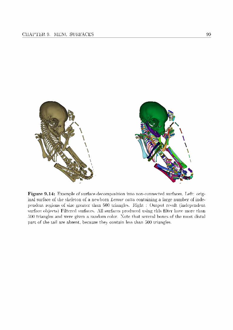
CHAPTER 9. MENU SURFACES 99
Figure 9.14: Example of surface decomposition into non-connected surfaces. Left: orig-inal surface of the skeleton of a newborn Lemur catta containing a large number of inde-pendent regions of size greater than 500 triangles. Right : Output result (independentsurface objects) Filtered surfaces. All surfaces produced using this �lter have more than500 triangles and were given a random color. Note that several bones of the most distalpart of the tail are absent, because they contain less than 500 triangles.

100 9.2. STRUCTURE MODIFICATION
Figure 9.15: Example of surface decomposition in order to keep largest region. Left:original 3D surface representing the skull of a newborn Tarsius bancanus. Right: theresulting largest region in terms of triangle number.
Figure 9.16: Example of surface inversion. Left: original surface of the skull of the typespecimen of Pan paniscus. Right: backface culling rendering of the same surface afterbeing inverted, revealing inner structures such as the endocranial cavity.

CHAPTER 9. MENU SURFACES 101
Figure 9.17: Example of fossil restoration (Palaeolemur betillei BOR613 specimen fromthe Musée d'Histoire Naturelle de Bordeaux, France) implicating the production of mirrorimages of missing parts.
9.3 Wrapping methods
9.3.1 Create a convex hull for each selected surface
This option uses vtkDelaunay3D. This �lter produces convex hull surfaces for each selectedsurface. Convex hulls can be useful for instance to compute estimations of the total "volume"occupied in space by complex objects containing lots of holes (see Fig. 9.18 p.102).
9.3.2 Shrink and wrap 1 surface over a 2nd surface
This option uses vtkSmoothPolyDataFilter to shrink a surface over the points of a second sur-face. Warning: the �rst (=impacted) surface should enclose the second (=observed) surface.This will approximately produce a convex hull of the observed object (see Fig. 9.19 p.102 andFig. 9.20 p.103).

102 9.3. WRAPPING METHODS
Figure 9.18: Convex hull computation. Left: original 3D surface representing the skullof a newborn Tarsius bancanus. Bone volume: ~100 mm3. Right: the resulting convexhull. Volume of the convex hull of the skull (=proxy for the volume of the "head"): ~3653mm3.
Figure 9.19: Shrink wrap dialog .

CHAPTER 9. MENU SURFACES 103
Figure 9.20: Convex hull computation. Left: A transparent sphere encloses the 3Dsurface representing the inner ear of a Galago moholi and (level . Right: the sphere wasskink-wrapped over the inner ear, resulting approximately in a convex hull.
9.4 Boolean operations
This option uses the vtkBooleanOperationPoly-DataFilter �lter. This �lter makes it possi-ble to perform boolean operations (subtraction,union and intersection) involving two surfaces(see for instance Fig. 9.22 p.104). Warning:this option works smoothly only when relatively"light surfaces" (less than a few thousand faces)are involved. Boolean operations on large freeform surface object will probably fail. SeevtkBooleanOperationPolyDataFilter documen-tation for further information.
Figure 9.21: Boolean operation dialog

104 9.4. BOOLEAN OPERATIONS
Figure 9.22: Example of possible boolean operations involving a sphere (surface A) anda cylinder of hexagonal section (surface B).

CHAPTER 9. MENU SURFACES 105
Figure 9.24: Example of alignment of two mandibles of Tarsius bancanus. A: the twosurfaces in their initial orientation. B: the two mandibles were roughly manually orientedin the same direction. C: result of the ICP algorithm. The impacted surface (the onewhich was actually reoriented) is the blue one.
9.5 Surface alignment
This option uses the vtkIterativeClosestPoint-Transform �lter. This �lter makes it possibleto align two surfaces using the Iterative ClosestPoint (ICP) algorithm. In order to get good re-sults, it is strongly advised to orient manuallyroughly the two surfaces in the same directionbefore running this algorithm (see for instanceFig. 9.24 p.105). See vtkIterativeClosestPoint-Transform documentation for further informa-tion.
Figure 9.23: Surface alignment dialog

106 9.6. RENDERING MODIFICATION
Figure 9.26: Edit color of all selected surfaces window.
9.6 Rendering modi�cation
9.6.1 Change transparency
All selected actors can be giventhe same transparency using thisoption (at least one selected surfaceis needed).Please choose a value between 0and 100. 100 stands for �opaquerendering". 0 stands for �invisiblesurface".
Figure 9.25: Edit transparency dialog
9.6.2 Change object solid color
Selected objects' solid color can be changed using the options that can be found inside thissubmenu. The "Custom color" option allows to de�ne a color to apply to all selected objects(see Fig. 9.26 p.106). Note that the transparency of all selected objects will remain unchanged.
Furthermore, a set of 13 prede�ned colors is available via this menu.
A last alternative is to edit all selected objects' colors and transparencies at once by usingthe �Default solid color of surfaces" control of the �Edit color options" window (menu �Edit→Edit color options").
9.7 Create 3D primitives
When planning to print a 3D model composed of non connex elements (for instance : thecranium and the mandible of a single individual, or the skeleton of the fetus of a vertebratespecimen), you may need to manually place in 3D space connective surface elements linkingthose di�erent parts. Such elements are referred to as "3D printing connective struts", andcan be created via the "Cylindric connective struts" dialog (Fig. 9.27 p.107) or via the "Cubicconnective struts" dialog (Fig. 9.30 p.110).

CHAPTER 9. MENU SURFACES 107
Figure 9.27: Create cylinders dialog. Di�erent options are available. Several cylinderssharing the same properties can be created at once. Shaft length and radius can bede�ned, as well as the resolution (number of sides). Also, shaft section shape can eitherbe circular or elliptical. The bottom and top sides of the cylinders can be either �at, orconic.
9.7.1 Create cylindric connective struts
Di�erent options are available, and in particular, the cylinders can be given either conic of �atends, and the cross-section of the cylinders can either be circular or elliptic (Fig. 9.28 p.108).Two practical examples of 3D printed objects using cylindric connective struts are shown inFig. 9.29 p.109.
9.7.2 Create cubic connective struts
Di�erent options are available, and in particular, the cubes / box-shaped struts can be givenany desired width, height and depth (see Fig. 9.30 p.110 and Fig. 9.31 p.110).
9.7.3 Create icosahedrons / spheres
Di�erent options are available, and in particular, the icosahedrons / spheres can be subdiviseda number of times, and their radius can be set as well(see Fig. 9.32 p.111 and Fig. 9.33 p.111).

108 9.7. CREATE 3D PRIMITIVES
Figure 9.28: Di�erent cylinder shapes. Top left: �at ends + circular shaft section.Top right: conic ends + circular shaft section. Bottom left: �at ends + elliptical shaftsection. Top right: conic ends + elliptical shaft section.

CHAPTER 9. MENU SURFACES 109
Figure 9.29: Examples of 3D connective material usage. A: Cranium and mandible ofGorilla gorilla (adult, male). Left: the 3D model of the skull is transparent, showingwhere the 3D connective cylinders have been placed in order to connect the mandible andthe cranium. Middle: the same 3D model is rendered opaque. Right: 3D printed object.B: 3D model of the skeleton of a newborn Lemur catta. The skeleton of this neonatespecimen contains many non connected elements: many bones are not fully mineralized(skull bones, vertebrae) and most bones are separated in space. Left: the 3D model ofthe skeleton is transparent, showing the position of the many cylinders (two hundreds) ofdi�erent lengths and diameters connecting the di�erent bones. Right: 3D printed object.

110 9.7. CREATE 3D PRIMITIVES
Figure 9.30: Create cube dialog. The X,Y and Z lengths of the cubic / box-shapedconnective struts can be de�ned here.
Figure 9.31: Example of cubic connective strut.

CHAPTER 9. MENU SURFACES 111
Figure 9.32: Create icosahedrons / spheres dialog. The number of subdivison, the radiusand the type of 3D primitive (icosahedron or sphere) are de�ned here.
Figure 9.33: Top line: from left to right: icosahedrons with subdivision levels of 0, 1,2 and 3 . Bottom line: from left to right: spheres with subdivision levels of 0, 1, 2 and3 .

112 9.8. SELECT SMALL OBJECTS
Figure 9.34: Select objects having a small number of triangles window.
Figure 9.35: Select surfaces having a small volume window.
9.8 Select small objects
This option permits to select all surface objects that contain less than a given number oftriangles (see Fig. 9.34 p.112). Selecting small objects can used subsequently to the surfacedecomposition tool, in order to remove small objects which are considered as not "relevant" oras "dirt" inside a complex 3D surface (see for instance Fig. 9.36 p.113) and that would havebeen hard to remove otherwise.
9.9 Select small volumes
This option is very similar to the one described just above, and permits to select all surfaceobjects, the volume of which is less than a given value(see Fig. 9.35 p.112). This way to selectobjects can used after the surface decomposition tool, in order to remove small objects whichare considered as not "relevant" or as "dirt" inside a complex 3D surface (see for instance Fig.9.36 p.113) and that would have been hard to remove otherwise.

CHAPTER 9. MENU SURFACES 113
Figure 9.36: A: A surface object (a cicada) is "dirty" and contains many non-relevantobjects which are not connected to the insect. B: The surface was decomposed intoindependant non-connected objects. C: Surface objects containing less than 5000 trianglesare selected and can then be removed by pressing "DEL". An alternative could have beento select all surface objects, the volume of which is less than a given value. D: All surfaceobjects containing less than 5000 triangles were removed. E: Two other larger and "non-relevant" objects were manually selected and deleted to further clean the cicada.

114 9.9. SELECT SMALL VOLUMES

Chapter 10
Menu Landmarks
Contents10.1 Edit �rst selected landmark . . . . . . . . . . . . . . . . . . . . . . . 116
10.2 Edit �rst selected �ag . . . . . . . . . . . . . . . . . . . . . . . . . . . 116
10.3 Select landmark range . . . . . . . . . . . . . . . . . . . . . . . . . . . 117
10.4 Selected landmarks: decrease landmark number (move up in list) 118
10.5 Selected landmarks: increase landmark number (move down in list)118
10.6 Selected landmarks: push back on closest surface's vertex . . . . . 118
10.7 Selected landmarks: change orientation according to surface's nor-mals . . . . . . . . . . . . . . . . . . . . . . . . . . . . . . . . . . . . . 118
10.8 Selected curve nodes and curve handle landmarks . . . . . . . . . . 120
10.8.1 Move curve handles semi-automatically . . . . . . . . . . . . . . . . . 120
10.8.2 Normal nodes (red): change as starting modes (dark green) . . . . . . 120
10.8.3 Normal nodes (red): connect to preceding starting nodes (cyan) . . . . 120
10.8.4 Normal nodes (red): de�ne as milestone (blue) . . . . . . . . . . . . . 120
10.8.5 Reset selected nodes to Normal nodes (red) . . . . . . . . . . . . . . . 120
10.9 Edit color of all selected �ag landmarks . . . . . . . . . . . . . . . . 124
10.10Edit length of all selected �ag landmarks . . . . . . . . . . . . . . . 124
10.11Update all selected �ag landmarks' color to that of the closestvertex . . . . . . . . . . . . . . . . . . . . . . . . . . . . . . . . . . . . 124
As stated above, landmarks can be set on surfaces by pressing �L" + left mouse click. Severalactions can be performed on landmarks.
115

116 10.1. EDIT FIRST SELECTED LANDMARK
Figure 10.1: Edit �rst selected landmark window.
10.1 Edit �rst selected landmark
This menu opens the "Edit �rst selected landmark" window (Fig. 10.1 p.116). in whichlandmark coordinates of landmarks can be manually edited. This window can also be opened
by clicking on " ". The center of rotation of the camera can be set to the x,y,z coordinatesof a given landmark by pressing on " ".
10.2 Edit �rst selected �ag
This menu opens the "Edit �rst selected �ag" window (Fig. 10.2 p.116), in which severalproperties of a given �ag can be manually edited.
- Flag name : modi�es the label of this �ag.- X, Y, Z: 3D coordinates of the �ag.- Next �ag and preceding �ag : saves currently settings and fetches next/preceding �ag- Flag color : modi�es the "color" of the currently selected �ag.- Flag rendering size : modi�es the length of the �ag.The center of rotation of the camera can be set to the x,y,z coordinates of a given �ag by
pressing on " ". Clicking on " " also opens this window.
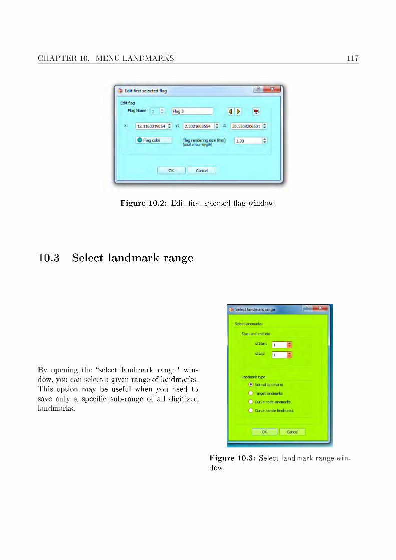
CHAPTER 10. MENU LANDMARKS 117
Figure 10.2: Edit �rst selected �ag window.
10.3 Select landmark range
By opening the �select landmark range" win-dow, you can select a given range of landmarks.This option may be useful when you need tosave only a speci�c sub-range of all digitizedlandmarks.
Figure 10.3: Select landmark range win-dow

11810.4. SELECTED LANDMARKS: DECREASE LANDMARK NUMBER (MOVE UP IN
LIST)
10.4 Selected landmarks: decrease landmark number (move
up in list)
This option will increase (=move up in list, if possible) the landmark number of all selectedlandmarks. This option can be also activated by clicking on in the "object controls" sectionof the main window.
10.5 Selected landmarks: increase landmark number (move
down in list)
This option will decrease (=move down in list, if possible) the landmark number of all selectedlandmarks. This option can be also activated by clicking on in the "object controls" sectionof the main window.
10.6 Selected landmarks: push back on closest surface's
vertex
When set via pressing �L" + left click, landmarks are always positioned at a surface's vertexcoordinates. Selected landmarks can be subsequently moved manually to other locations (forinstance, if you want to place a given landmark in the middle of a canal or of a foramen, orbetween two unfused bones). However, you may sometimes want to push back automaticallysome selected landmarks to the position of the closest surface's vertex available. This can beachieved using this option (see for instance Fig. 10.4 p.119).
10.7 Selected landmarks: change orientation according to
surface's normals
When set via pressing �L" + left surfaces, landmark orientation is that of the vertex on whichit is placed. Selected landmarks' orientation can be subsequently moved manually. However,you may sometimes want to reset one or several landmarks' orientation automatically to thatof the normal of the closest surface's vertex available. This can be achieved using this option(see for instance Fig. 10.5 p.119).

CHAPTER 10. MENU LANDMARKS 119
Figure 10.4: Push back selected landmarks on surface's closest vertex. A: two landmarks(4 and 5) laying outside the surface of the left inner of a Galago moholi specimen have beenselected. B: these 2 landmarks now lay on the surface. This action can be undone/redone.
Figure 10.5: Change orientation according to surface's normals. A: two landmarks (4and 5) the surface of the left inner of a Galago moholi specimen have been selected. B:these 2 landmarks' orientation now is the same as that of the closest vertices. This actioncan be undone/redone.

120 10.8. SELECTED CURVE NODES AND CURVE HANDLE LANDMARKS
10.8 Selected curve nodes and curve handle landmarks
Before reading this paragraph, in order to get a good understanding about how curves areconstructed in MorphoDig, please make sure you have read carefully the section 7.5 p.59.
10.8.1 Move curve handles semi-automatically
This option allows saving a lot of time whencreating 3D Bezier curves with MorphoDig (seeFig. 10.7 p.121). Also see �working with curves"tutorial for further details regarding curve dig-itization with MorphoDig).
Figure 10.6: Mode handles windowRequirement : at least a handle landmark (�purple" landmark) must be selected. Depending
on whether selected curve handles lie within the curve, at the start of the curve or at the endof the curve, their displacements di�er (see Fig. 10.8 p. 122)
10.8.2 Normal nodes (red): change as starting modes (dark green)
This option makes it possible to decompose a "long" curve passing through a given numberof curve nodes into distinct "independent" curve segments. A practical example is shown inFig. 10.9 p. 122. Selected node landmarks will be given �ag �1". Please also refer to section7.5 p.59.
10.8.3 Normal nodes (red): connect to preceding starting nodes (cyan)
This option makes it possible to "close" curve segments by connecting the last node of a curvesegment to the starting point of that curve segment. A practical example is shown in Fig. 10.10p. 123. Selected node landmarks will be given �ag �3". Please also refer to section 7.5 p.59.
10.8.4 Normal nodes (red): de�ne as milestone (blue)
This option makes it possible to decompose a curve passing through a given number of curvenodes into "contiguous" curve segments. A practical example is shown in Fig. 10.11 p. 123.Each curve milestone is involved into 2 curve segments: it acts as the ending node of a givencurve, and as the starting point of the following curve. Curve milestones are given �ag �2".
10.8.5 Reset selected nodes to Normal nodes (red)
Special nodes (curve starting points, nodes connected to their preceding starting points, andcurve milestones) are reset back to a "normal" state when using this option. Selected landmark
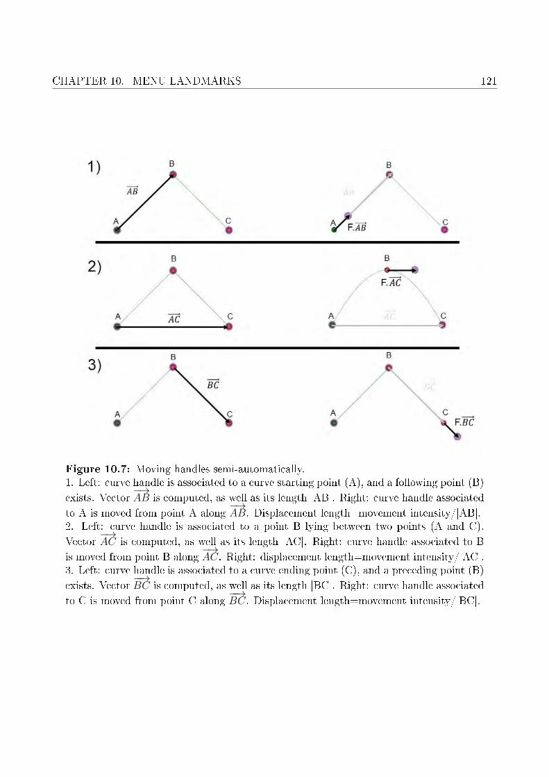
CHAPTER 10. MENU LANDMARKS 121
Figure 10.7: Moving handles semi-automatically.1. Left: curve handle is associated to a curve starting point (A), and a following point (B)
exists. Vector−→AB is computed, as well as its length |AB|. Right: curve handle associated
to A is moved from point A along−→AB. Displacement length=movement intensity/|AB|.
2. Left: curve handle is associated to a point B lying between two points (A and C).
Vector−→AC is computed, as well as its length |AC|. Right: curve handle associated to B
is moved from point B along−→AC. Right: displacement length=movement intensity/|AC|.
3. Left: curve handle is associated to a curve ending point (C), and a preceding point (B)
exists. Vector−−→BC is computed, as well as its length |BC|. Right: curve handle associated
to C is moved from point C along−−→BC. Displacement length=movement intensity/|BC|.

122 10.8. SELECTED CURVE NODES AND CURVE HANDLE LANDMARKS
Figure 10.8: Example of curve handles semi-automatic displacement (movement inten-sity: 25%).
Figure 10.9: Curve decomposition into segments (left bony labyrinth of Galago moholi).Left: a single curve passes through 15 curve node landmarks. Right: curve node n◦10was de�ned as a new curve starting point. Now, there are two curves. The �rst curvepasses through the cochlea only (nodes 1 to 9). The second one passes through the lateralsemicircular canal (nodes 10 to 15).

CHAPTER 10. MENU LANDMARKS 123
Figure 10.10: Closing curve segments (left bony labyrinth of Galago moholi). Left: thecurve segment passing through the lateral semicircular canal is "open": the curve doesnot pass through the �rst curve node (node n◦10) and the last one (node n◦15). Right:curve node n◦15 was connected to the preceding curve starting node n◦10. Now, the curvepassing through the lateral semicircular canal is "closed".
Figure 10.11: Curve decomposition into contiguous segments (left bony labyrinth ofGalago moholi). Left: curve 1 (nodes 1-9) passes through the cochlea; curve 2 passesthrough the lateral semicircular canal (nodes 10-15). Right: curve nodes 4 and 12 werede�ned as curve milestones. When exporting curve infos or landmarks, MorphoDig nowconsiders that 4 curve segments exist: curve 1 (nodes 1-4); curve 2 (nodes 4-9); curve 3(nodes 10-12); curve 4 (nodes 12-15).

124 10.9. EDIT COLOR OF ALL SELECTED FLAG LANDMARKS
are given �ag �0".Further information regarding curve use in MorphoDig is available in the section �File →Curves" section (section 7.5 p.59) and in the tutorial �working with curves".
10.9 Edit color of all selected �ag landmarks
Using this option, you can modify the color ofall selected �ag landmarks at once.
Figure 10.12: Edit color of all selected�ags dialog
10.10 Edit length of all selected �ag landmarks
Using this option, you can modify the length ofall selected �ag landmarks at once.
Figure 10.13: Edit length of all selected�ags dialog
10.11 Update all selected �ag landmarks' color to that of
the closest vertex
This option will set the color of all selected �ag landmarks to that of the closest vertex foundin all opened surface objects. A practical example is shown in Fig. 10.14 p. 125.
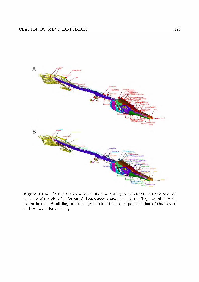
CHAPTER 10. MENU LANDMARKS 125
Figure 10.14: Setting the color for all �ags according to the closest vertices' color ofa tagged 3D model of skeletton of Atractosteus tristoechus. A: the �ags are initially alldrawn in red. B: all �ags are now given colors that correspond to that of the closestvertices found for each �ag.

12610.11. UPDATE ALL SELECTED FLAG LANDMARKS' COLOR TO THAT OF THE
CLOSEST VERTEX

Chapter 11
Menu Scalars
Contents11.1 Open scalars window . . . . . . . . . . . . . . . . . . . . . . . . . . . 128
11.2 Compute distance from camera for each selected surface . . . . . . 131
11.3 Compute thickness within each selected surface . . . . . . . . . . . 136
11.4 Compute thickness between two surfaces . . . . . . . . . . . . . . . 137
11.5 Compute distance between two surfaces . . . . . . . . . . . . . . . . 138
11.6 Compute curvature for each selected surface . . . . . . . . . . . . . 138
11.7 Compute complexity for each selected surface . . . . . . . . . . . . 139
11.7.1 Local Convex hull Area Ratio (LCh-AR) . . . . . . . . . . . . . . . . . 141
11.7.2 Local Sphere Area Ratio (LS-AR) . . . . . . . . . . . . . . . . . . . . 141
11.7.3 Local Convex hull Normalized Shape Index (LCh-NSI) . . . . . . . . . 142
11.7.4 Local Sphere Normalized Shape Index (LS-NSI) . . . . . . . . . . . . . 142
11.8 Smooth active scalars for each selected surface . . . . . . . . . . . . 144
11.9 Normalize or rescale active scalars for each selected surface . . . . 144
Simple numeric quantities (=numbers, or "scalar values") can be associated to each vertexof a given surface, and are referred to as "scalar arrays" in this section. As stated earlier, a givenunselected surface can be colored using the currently active scalar array, if that surface containsthat scalar array (see also Fig. 4.2-B p.21). To do so, the array display mode button must
be pressed ( ), and a scalar array must be selected as the currently active array (ex: ).The way scalar arrays are translated into colors can be set up using color maps, also referredto as "Lookup tables" (LUT) or color transfer functions.
127

128 11.1. OPEN SCALARS WINDOW
11.1 Open scalars window
The "Scalars" window can be opened by clicking on " " (see Fig. 11.1).Available controls:1: Active scalar array: choose among the available scalars the one which will be displayed.
2: Remove selected scalar array: deletes currently active scalar array from all openedsurfaces, or from selected surfaces only. This option is useful if you plan to save surfaces in the.vtk format and do not want MorphoDig to save associated scalar values (this will save somedisk space).
3: Active color map: choose among currently available colormaps. See Fig. 11.2 for apractical example.
4: Color map controls: Four buttons areavailable. a:reinitialize color map (only possiblefor the 2 �rst prede�ned color maps). b: exportcolor maps(s). When clicked, the export colormap(s) dialog shows up (see Fig. 11.3), inwhich you may de�ne more precisely the colormap(s) that should be exported. c: changeactive color map name (can be only done oncustom color maps). d: delete active color map(only custom color maps can be deleted).
Figure 11.3: Export color maps dialog.
5: Opacity control points : opacity control points of the active color map. Such controlpoints can be added (left click on a line), deleted (select one control point using the left mousebutton then press "delete") and edited (drag one control point using the left mouse button)interactively.
6: Color control points : color control points of the active color map. Such control pointscan be added (left click on an empty zone), deleted (select one control point using the left mousebutton then press "delete") and edited (drag one control point using the left mouse button)interactively.
7: additional color map controls. From top to bottom. a: set colormap range to matchthe global active scalar min and max found for all currently opened surfaces. b: reverse colorcolor control points (see Fig. 11.4). c: reverse opacity control points (see Fig. 11.5). d: Save

CHAPTER 11. MENU SCALARS 129
Figure 11.1: Scalar control window. This window is divided in di�erent subsections. 1)choose current 3D rendered scalar array. 2) the active scalar array can be deleted fromselected/all surface objects in this sections. 3) choose current active color map, whichtransforms numbers into color and opacity on the screen. 4) operations on the activecolormap. a: reinitialize color map. b: change active color map name. c: delete activecolor map. 5) opacity control points of the active color map. 6) color control points ofthe active color map. 7) modi�cation controls of the active color map. a: set range tomin and max. b: reverse color control points. c: reverse opacity control points. d: exportcolors map(s) inside a .MAP �le. e: Save to preset = duplicate current active color mapand create a new custom color map. 8) enable/disable opacity mapping. 9) discretizecolor levels, and choose number of levels. 10) shif both min and max, or change displayedmin and max of color map. 11) set min and max of color map based on suggested values.These suggested min and max values are computed in order to remove a percentage ofmost extreme minimal and maximal values found in the vertices of all opened surface forthe active scalar.

130 11.1. OPEN SCALARS WINDOW
Figure 11.2: Example of active colormap modi�cation. Left: left inner ear of Galagomoholi. Active scalars: thickness. Colormap: rainbow. Right: the same inner ear afterthe active colormap has been set to "Black-red-white".

CHAPTER 11. MENU SCALARS 131
to preset = duplicate current active color map and create a new custom color map.duplicatecurrent active color map and create a new custom color map.
8: enable/disable opacity mapping. When opacity mapping is disabled, all surface objectsare rendered using their "global" transparency level.
9: discretize color levels, and choose number of levels. See Fig. 11.6 for a practical example.
10: change min and max of color map. You may use these sliders to change the minimaland maximal values of the active color map. By default, all colormaps range between 0 (min)and 1 (max), which may not be the most appropriate range to display a given scalar array.
11: set min and max of color map based on suggested values. As stated above, bydefault, all colormaps range between 0 (min) and 1 (max), which may not be the most appro-priate range to display a given scalar array. You may set the minimal and maximal values ofthe active colormap based on suggested values, which are computed automatically based on thecurrently opened surface objects, and which are computed in order to use the color scale at itsbest. See Fig. 11.7 for a practical example.
11.2 Compute distance from camera for each selected sur-
face
Computes distance (=depth) from camera for all vertices of all selected surfaces. This optionmay o�er a better perception of the 3D structure of an object on a 2D screen representation.This option also makes it possible to compute an elevation map. See Fig. 11.8 for a practicalexample.

132 11.2. COMPUTE DISTANCE FROM CAMERA FOR EACH SELECTED SURFACE
Figure 11.4: Example of color inversion of a colormap. Left: left inner ear of Galagomoholi. Active scalars: thickness. Colormap: rainbow. Right: the same inner ear afterthe color control points of the rainbow colormap have been reversed.

CHAPTER 11. MENU SCALARS 133
Figure 11.5: Example of opcacity inversion of a colormap. Left: left inner ear of Galagomoholi. Active scalars: thickness. Colormap: rainbow. Right: the same inner ear afterthe opacity leveles of the rainbow colormap have been reversed.

134 11.2. COMPUTE DISTANCE FROM CAMERA FOR EACH SELECTED SURFACE
Figure 11.6: Example of colormap discretization. Left: left inner ear of Galago mo-
holi. Active scalars: thickness. Colormap: custom. Right: the same inner ear after the"discretize" option has been turned on, and the nr of values set to 10.

CHAPTER 11. MENU SCALARS 135
Figure 11.7: Example of suggested min and max usage. Left: Left inner ear of Galagomoholi. Active scalars: thickness. Colormap: rainbow. Te rainbow colormap is set asby default to range between 0 (min) and 1 (max). Right: the same inner ear after therainbow colormap range has been modi�ed based on suggested min (0.16) and suggestedmax (0.91) values.

136 11.3. COMPUTE THICKNESS WITHIN EACH SELECTED SURFACE
Figure 11.8: Example of camera distance scalar array. Displayed specimen: upper outerenamel surface of a second upper molar of Homo sapiens.
11.3 Compute thickness within each selected surface
Thickness within an object (see Fig. 11.9) isde�ned the following way: for a given vertex,the minimal distance between this vertex andother vertices in the direction opposite to thatof the surface's normal. In order to minimizecomputation time, a maximal distance (Maxi-mal thickness (size unit) ) is asked to the user,in order to reduce the amount of vertices in-vestigated at a given location. Also, in order toavoid to take into account only relevant verticesin that computation, an angular limit betweeninvestigated vertex normals (by default: 70◦)is asked. Finally, a smoother scalar array out-put can be produced by setting the "thickness"value as the average of the distance found be-tween a number of closest vertices found. SeeFig. 11.10-A for a practical example.
Figure 11.9: Thickness within a givensurface.

CHAPTER 11. MENU SCALARS 137
Figure 11.10: Examples of thickness computation. A: thickness within object. Spec-imen: left inner ear of Galago moholi. B: thickness between the outer enamel surface(OEJ) and the enamel-dentine junction (EDJ) of a second upper molar of Homo sapiens.
11.4 Compute thickness between two surfaces
Thickness between two objects is de�ned thefollowing way (see Fig. 11.11): for a given ver-tex of the impacted object, the minimal dis-tance between this vertex and other verticesof the observed surface in the same direction(if "invert normals of observed object" optionis unchecked) or in the opposite direction (if"invert normals of observed object" option ischecked) to that of the impacted surface's nor-mal is computed. Again, in order to minimizecomputation time, a maximal distance (Maxi-mal thickness (size unit) ) is asked to the user,in order to reduce the amount of vertices in-vestigated at a given location. Also, in order toavoid to take into account only relevant verticesin that computation, an angular limit betweeninvestigated vertex normals (by default: 70◦)is asked. Finally, a smoother scalar array out-put can be produced by setting the "thickness"value as the average of the distance found be-tween a number of closest vertices found. SeeFig. 11.10-B for a practical example.
Figure 11.11: Thickness between 2 sur-faces window
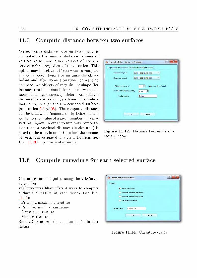
138 11.5. COMPUTE DISTANCE BETWEEN TWO SURFACES
11.5 Compute distance between two surfaces
Vertex closest distance between two objects iscomputed as the minimal distance between allvertices vertex and other vertices of the ob-served surface, regardless of the direction. Thisoption may be relevant if you want to comparethe same object twice (for instance the objectbefore and after some alteration) or want tocompare two objects of very similar shape (forinstance two inner ears belonging to two speci-mens of the same species). Before computing adistance map, it is strongly advised, in a prelim-inary step, to align the two compared surfaces(see section 9.5 p.105). The computed distancecan be somewhat "smoothed" by being de�nedas the average value of a given number of closestvertices. Again, in order to minimize computa-tion time, a maximal distance (in size unit) isasked to the user, in order to reduce the amountof vertices investigated at a given location. SeeFig. 11.13 for a practical example.
Figure 11.12: Distance between 2 sur-faces window
11.6 Compute curvature for each selected surface
Curvatures are computed using the vtkCurva-tures �lter.vtkCurvatures �lter o�ers 4 ways to computesurface's curvature at each vertex (see Fig.11.15):- Principal maximal curvature- Principal minimal curvature- Gaussian curvature- Mean curvature.See vtkCurvatures' documentation for furtherdetails.
Figure 11.14: Curvature dialog

CHAPTER 11. MENU SCALARS 139
Figure 11.13: Example of distance map between two surfaces. An inner ear of Galagomoholi was virtually distorted in the lateral canal region. The corresponding representa-tion of the deformation is shown here using a distance map: in red can we identify themost distorted regions.
11.7 Compute complexity for each selected surface
In section 7.10.2 p.69 and section 7.10.3 p.70, proxies for shape complexity (= how much areacan be enclosed within a given volume) are described. The limit of those approaches is thatthey produce single values for a whole surface, and do not take into account shape variationwithin surfaces. However, a single biological object can express a lot of shape variability.In this section, we extend the approach of shape complexity described earlier: we providesurface complexity measurements for all vertices of a surface. To do so, for each vertex, alocal surrounding area is extracted and shape complexity is measured for this local area. Theconsequence of this approach is that these measurements depend on the extent of the local areainvestigated for each vertex. For a given surface, the "local" area investigated is a sphere ofradius "R". By default, for a given surface, R is computed as follows:
R =Avg(length(PC1) + length(PC2) + length(PC3)))
18(11.1)
The numerator of this equation is in our view a sensible estimate of the "average extension"of an object in 3D space. It is computed as is the average of the lengths of a given objectalong its 3 principal extension axes. This measurement is obtained by performing a principalcomponent analysis on the vertex coordinates of a given surface. The denominator (18) is setempirically, as it seems to provide a reasonable estimate of "locality" for all vertex locations,

140 11.7. COMPUTE COMPLEXITY FOR EACH SELECTED SURFACE
Figure 11.15: Examples of 3D rendering of �Curvature" scalars. Scalar mode is active,the rainbow color scale is used. Specimen: enamel dentine junction (EDJ) of the secondsuperior molar of Neolithic human of the necropolis of Gurgy (France). Image credit:Mona Le Luyer.

CHAPTER 11. MENU SCALARS 141
Figure 11.16: Complexity dialog.
regardless the global shape of the investigated surfaces. However, R can be set to a customvalue in the Scalars complexity dialog (see Fig. 11.16).
Four complexity measurements are provided:
11.7.1 Local Convex hull Area Ratio (LCh-AR)
For each vertex V, the surrounding surface's local region enclosed within an area de�ned bya local sphere of center V and radius R is extracted. Then the local convex hull normalizedarea ratio (ChAR) is computed for this local region. ChAR is de�ned as the ratio betweenthe extracted local surface area and the surface area of the convex hull computed for the sameextracted local surface.This measurement of surface complexity takes more time to compute (computation of a Convexhull for each vertex) than the LS-AR and LS-NSI indices (see below) based on the local sphere,but it has two advantages (see Fig. 11.17-B p.11.17):- very low "border" artifacts (complex structures located at the outskirts of surfaces are givenhigh complexity values).- contrary to the LCh-NSI index (see below), isolated very �at (and non-complex) structuresare given, as they should be, low complexity values .
11.7.2 Local Sphere Area Ratio (LS-AR)
For each vertex V, the surrounding surface's local region enclosed within an area de�ned by alocal sphere of center V and radius R is extracted. Then complexity is computed as the ratiobetween the area of the extracted surface and the area of the sphere of radius R.
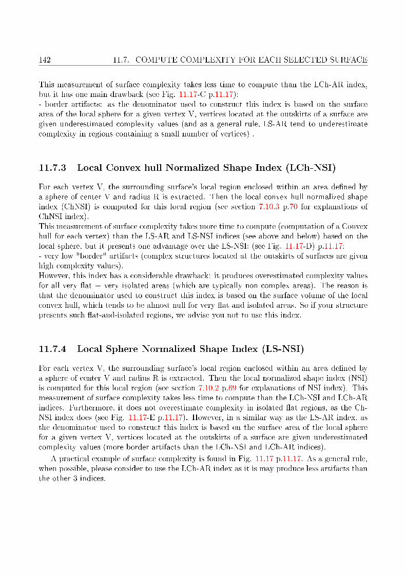
142 11.7. COMPUTE COMPLEXITY FOR EACH SELECTED SURFACE
This measurement of surface complexity takes less time to compute than the LCh-AR index,but it has one main drawback (see Fig. 11.17-C p.11.17):- border artifacts: as the denominator used to construct this index is based on the surfacearea of the local sphere for a given vertex V, vertices located at the outskirts of a surface aregiven underestimated complexity values (and as a general rule, LS-AR tend to underestimatecomplexity in regions containing a small number of vertices) .
11.7.3 Local Convex hull Normalized Shape Index (LCh-NSI)
For each vertex V, the surrounding surface's local region enclosed within an area de�ned bya sphere of center V and radius R is extracted. Then the local convex hull normalized shapeindex (ChNSI) is computed for this local region (see section 7.10.3 p.70 for explanations ofChNSI index).This measurement of surface complexity takes more time to compute (computation of a Convexhull for each vertex) than the LS-AR and LS-NSI indices (see above and below) based on thelocal sphere, but it presents one advantage over the LS-NSI: (see Fig. 11.17-D) p.11.17:- very low "border" artifacts (complex structures located at the outskirts of surfaces are givenhigh complexity values).However, this index has a considerable drawback: it produces overestimated complexity valuesfor all very �at + very isolated areas (which are typically non complex areas). The reason isthat the denominator used to construct this index is based on the surface volume of the localconvex hull, which tends to be almost null for very �at and isolated areas. So if your structurepresents such �at-and-isolated regions, we advise you not to use this index.
11.7.4 Local Sphere Normalized Shape Index (LS-NSI)
For each vertex V, the surrounding surface's local region enclosed within an area de�ned bya sphere of center V and radius R is extracted. Then the local normalized shape index (NSI)is computed for this local region (see section 7.10.2 p.69 for explanations of NSI index). Thismeasurement of surface complexity takes less time to compute than the LCh-NSI and LCh-ARindices. Furthermore, it does not overestimate complexity in isolated �at regions, as the Ch-NSI index does (see Fig. 11.17-E p.11.17). However, in a similar way as the LS-AR index, asthe denominator used to construct this index is based on the surface area of the local spherefor a given vertex V, vertices located at the outskirts of a surface are given underestimatedcomplexity values (more border artifacts than the LCh-NSI and LCh-AR indices).
A practical example of surface complexity is found in Fig. 11.17 p.11.17. As a general rule,when possible, please consider to use the LCh-AR index as it is may produce less artifacts thanthe other 3 indices.

CHAPTER 11. MENU SCALARS 143
Figure 11.17: Local complexity scalar computed in turbinate bones of Orycteropus afer.A. Left endo, naso and maxillo turbinate bones viewed from the left side. Left-to-right:antero-posterior direction. Bottom-up: dorso-ventral direction. B: the Local Convex hullArea Ratio (LCh-AR) presents two advantages: no "border" artifacts, and no overestima-tion of complexity in �at-isolated regions. C: the Local Sphere Area Ratio (LS-AR) tendsto underestimate complexity at the outskirts of complex structures ("border artifacts",see black arrows). D: the Local Convex hull Normalized Shape Index (LCh-NSI) tendsto overestimate complexity is some very �at and isolated areas. See for instance the redareas in the center of the nasoturbinate and in the anterior part of the endoturbinate(black arrows). E: Local Sphere Normalized Shape Index (LS-NSI) presents no overesti-mation of complexity in �at-isolated regions, but tends to underestimate complexity atthe outskirts of complex structures ("border artifacts", see black arrows). Image courtesy:Lionel Hautier and Mark Wright.

144 11.8. SMOOTH ACTIVE SCALARS FOR EACH SELECTED SURFACE
Figure 11.18: Scalar smoothing dialog. Smoothing can be computed using only directneighbor vertices. A much larger area can also be investigated to produce a "smoothed"output. A percentage of extreme minimal and maximal values found can be excluded fromthe smoothing process. Also, the "smoothed" output can be computed as the average oras the median of the scalar values found for the neighbor vertices.
11.8 Smooth active scalars for each selected surface
It may happen that scalar values contain a lot of noise (see for instance the noisy results of thecurvature computation in Fig. 11.15). In order to reduce noise and retrieve more biologicallyrelevant information, scalars can be �smoothed" in di�erent ways (see 11.18). Be aware thatthe obtained results depend very much on the size of the investigated local area for each vertex(based on direct neighbor vertices or on a much larger area), and on whether the new scalarvalue is computed as the average or as the median of the scalar values found for neighborvertices (see Fig. 11.19).
11.9 Normalize or rescale active scalars for each selected
surface
It may be useful to normalize scalar values between 0 and 1, or to rescale them for di�erentpurposes. For instance, scalar normalization makes it possible to compare scalar arrays of

CHAPTER 11. MENU SCALARS 145
Figure 11.19: Smoothing scalars. Examples of 3D rendering of �Min Curvature" scalars.Top : "raw" minimal curvature, which is extremely variable locally, and hard to interpret.Middle line: averaging direct neighbors or averaging scalar values on a much larger areagive di�erent results. See also how much averaging scalar values is sensitive with extrememin and max values. Bottom line : computing a median based upon direct neighborsor upon scalar values found within a much larger area also give di�erent results. Themedian smoothing "method"' is much less sensitive with extreme values (no di�erenceseen when only 1% of the most extreme min and max values are removed). Specimen:enamel dentine junction (EDJ) of the second superior molar of a Neolithic human of thenecropolis of Gurgy (France). Image credit: Mona Le Luyer.

14611.9. NORMALIZE OR RESCALE ACTIVE SCALARS FOR EACH SELECTED
SURFACE
di�erent nature (and having very di�erent min-max ranges) using a unique color scale rangingbetween 0 and 1. Also, in order to be able compare scalars such as bone thickness or enamelthickness variation between specimens of very di�erent size, scalar normalization is a necessarystep. The scalar normalization/rescale dialog is shown in Fig. 11.20 p.147. An example ofnormalization of di�erent scalars within a single surface is shown in Fig. 11.21 p.148. Anexample of normalization of a single scalar in order to compare di�erent specimens is shown inFig. 11.22 p.149.

CHAPTER 11. MENU SCALARS 147
Figure 11.20: Scalar normalization/rescale dialog. The "old min" and "old max" valuerepresent by default the minimal and maximal value of the active scalars within all cur-rently opened surfaces. After the scalar normalization/rescale has been performed, "oldmin" will have been set to "new min", "old max" will have been set to "new max", andscalar values in between "old min" and "old max" will range between "new min" and"new max" using a linear interpolation. "old min" and "old max" can be given othervalues than the real min and max of the active scalar via two options. 1) a given percent-age of extreme min and max values can be removed from the current active scalar values(sometimes only a few extreme "strange" values can give a wrong idea of the "real" extantof the range of a given scalar). 2) if the "custom old min/max" option is checked, oldmin and old max values can be set to any value. When one of these two options is used,the interpolated values produced may fall above "new max" or below "new min". Thenyou may decide whether you allow such "out of the range" values using the "allow < newmin" and "allow > new max" options. If unchecked, interpolated values falling below"new min" will be set to "new min", and interpolated values falling above "new max"will be set to "new max". The "�ip output" option will reverse the range of interpolatedvalues between "new min" and "new max".

14811.9. NORMALIZE OR RESCALE ACTIVE SCALARS FOR EACH SELECTED
SURFACE
Figure 11.21: Normalization of di�erent scalars within the same specimen. All illustra-tions use the same color table, ranging between 0 and 1. A : "Minimal curvature". B :"Maximal curvature". C : "Mean curvature". D : "Gaussian curvature". Top line: "raw"4 scalars, which all express a lot of noise. Middle line: the 4 same "smoothed"' scalarsafter a median �lter has been used. Bottom line: the 4 same scalars after normalization.The 5% most extreme minimal values and maximal values have been excluded from thisnormalization process, because they are clearly aberrant (most values range between -10and 10 for all 4 raw scalars, but a few outliers have values above 10000 and below -10000).The visual output of the bottom line is easier to interpret. Specimen: enamel dentinejunction (EDJ) of the second superior molar of a Neolithic human of the necropolis ofGurgy (France). Image credit: Mona Le Luyer.
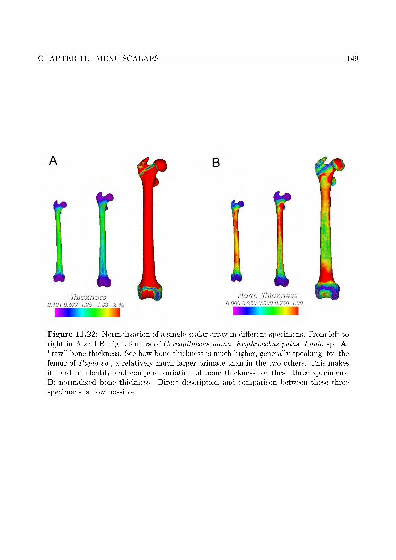
CHAPTER 11. MENU SCALARS 149
Figure 11.22: Normalization of a single scalar array in di�erent specimens. From left toright in A and B: right femurs of Cercopithecus mona, Erythrocebus patas, Papio sp. A:"raw" bone thickness. See how bone thickness is much higher, generally speaking, for thefemur of Papio sp., a relatively much larger primate than in the two others. This makesit hard to identify and compare variation of bone thickness for these three specimens.B: normalized bone thickness. Direct description and comparison between these threespecimens is now possible.

15011.9. NORMALIZE OR RESCALE ACTIVE SCALARS FOR EACH SELECTED
SURFACE
Chapter 12
Menu Tags
Contents12.1 Open Tags window . . . . . . . . . . . . . . . . . . . . . . . . . . . . . 152
12.2 Create new empty tag array for each selected surface . . . . . . . . 152
12.3 Create new tag array based on currently displayed colors for eachselected surface . . . . . . . . . . . . . . . . . . . . . . . . . . . . . . . 152
12.4 Create new tag array based on connectivity for each selected surface155
12.5 Extract active tag region for each selected surface . . . . . . . . . . 155
12.6 Extract tag region range for each selected surface . . . . . . . . . . 155
12.7 Extract each tag region as a new object, for all tag regions of allselected surfaces . . . . . . . . . . . . . . . . . . . . . . . . . . . . . . 156
12.8 Tagging with MorphoDig: a quick starting guide . . . . . . . . . . 156
12.8.1 Pencil tag tool . . . . . . . . . . . . . . . . . . . . . . . . . . . . . . . 159
12.8.2 Paint bucket tag tool . . . . . . . . . . . . . . . . . . . . . . . . . . . . 159
12.8.3 Lasso tag tool . . . . . . . . . . . . . . . . . . . . . . . . . . . . . . . . 160
12.8.4 Rubber band tag tool . . . . . . . . . . . . . . . . . . . . . . . . . . . 160
12.8.5 Merge tag regions . . . . . . . . . . . . . . . . . . . . . . . . . . . . . . 160
All vertices of di�erent biological structures can be given a speci�c integer values (0, 1, 2,3 ...), in order to identify them. Such integer arrays are referred to as "tag arrays". As statedearlier, a given unselected surface can be colored using the currently active tag array (identi�edby its "name"), if that surface contains a tag array of that name (see also Fig. 4.2-B p.21). To
do so, the array display mode button must be pressed ( ), and a tag array must be selected as
the currently active array (ex: ). The way tag arrays are translated into colors can beset up using tag maps, also referred to as "Lookup tables" (LUT) or color transfer functions.
151

152 12.1. OPEN TAGS WINDOW
Contrary to "scalar arrays" (see preceding section), tags are usually drawn manually with"painting tools".For convenience purposes, as selected surfaces are drawn "grey" in MorphoDig, unselectedsurfaces objects can be tagged (tagging uniform "grey" objects without visual feedback wouldbe uneasy). Tagging is the only way to modify an unselected surface in MorphoDig.In order to be able to edit tags on a surface, the most common way is to create a new emptytag array for this surface (see section 12.2 p. 12.2 for further details). You may read section12.8 p.156 for a quick tagging starting guide.
12.1 Open Tags window
The "Tags" window can be also opened by clicking on " " (see Fig. 12.1). The Tags windowcontains most options related to tags. The active tag array can be chosen here, as well asthe active tag map. Tag maps (name, color, opacity of di�erent biological structures) can bede�ned and modi�ed here as well. The currently used tag tool is also chosen in this window
(pencil " ", paint bucket " ", lasso " " or rubber band " ").
12.2 Create new empty tag array for each selected surface
This option will create a new "empty" tag ar-ray (the name of this new array is given by theuser). "Empty", in this context, means thatall vertices are assigned to the "Exterior" tag(tag=0).
Figure 12.2: Creating a new tag array
12.3 Create new tag array based on currently displayed
colors for each selected surface
Advice: do not use this method on surfaces displayed with color gradients. This optionusually only makes sense when distinct colors are displayed (typically: less than 30).This option (see Fig. 12.3) may be useful when you just have opened a .ply �le alreadycontaining RGB colors (for instance, let us suppose that you have painted a surface usingMeshLab software, and that you wish to convert those colors into tags). RGB colors containedin .ply �les are inserted inside the RGB array when opened with MorphoDig. This option is not

CHAPTER 12. MENU TAGS 153
Figure 12.1: Tags window. This window is divided in di�erent subsections. 1) choosecurrent active tag array. 2) the active tag array can be deleted from selected/all surfaceobjects in this sections. 3) choose current active tag map, which transforms integer valuesinto color and opacity on the screen. 4) operations on the active tag map (from left toright). a: reinitialize tag map. b: Add tag map to presets = duplicate current active tagmap and create a new custom tag map. c: export tag map(s) inside a .TAG or .TGP �le.d: change active color map name (only possible for custom tag maps). d: delete activecolor map (only possible for custom tag maps). 5) active tag tools (from left to right): a:pencil. b: paint bucket. c: lasso tag. d: rubber band tag. Di�erent options are availablefor the pencil tool. Pencil radius size (in pixels rendered on the screen). Pencil limit angle(in degrees). Tag all vertices within radius or propagate from picked location (relevant tostop tag propagation at topological boundaries; can be used in conjunction with a limitangle below 180 degrees). 6) The tag map table: each line of this table (= each tag region)is associated with an integer (exterior: 0; Tag1: 1 etc.), a color and an opacity. The activetag tools will paint a surface using the active tag region. 7) modi�cation controls of theactive tag map (from left to right). a: add a line to tag map table. b: remove last linefrom tag map table. c: reset active tag region (merge with Tag 0 = Exterior). d: mergetwo tag regions.

15412.3. CREATE NEW TAG ARRAY BASED ON CURRENTLY DISPLAYED COLORS
FOR EACH SELECTED SURFACE
Figure 12.3: Create Tag array from RGB array.
restricted to RGB arrays contained inside .ply �les though: it is also possible to convert anydisplayed color (such as scalar color rendering via a discretized color table) into a tag value.
Two main ways to convert currently displayed colors are available :1) Exact color match using active tag map→ In that case, in order to be given a tag value other than Tag 00, a vertex must satisfy thefollowing condition: its RGB scalar value should match one of the colors de�ned in the "Tagsoptions" window for the active tag map. If a vertex does not satisfy this condition, it is giventhe Tag 00 value (=exterior).2) De�ne tags following the �rst N distinct colors found→ In that case the following sequence of operations is performed:a) Important: MorphoDig re-initializes the currently active tag map. If you have spent timeto de�ne colors and labels on the currently active tag map, it is strongly advised to save theactive tag map inside a .TAG or .TGP �le in order to be able to re-load it later. Otherwise,your work will be lost.b) MorphoDig inspects the RGB display color of all the vertices of opened surfaces. Whenmeeting a new color, if the active tag map contains less than "N" lines, MorphoDig inserts anew line inside the active tag map (of that color), and associates the current vertex id to thisnew tag id entry. All vertices of that same color will be associated to that id. If the color ofthe vertex is "new" and the maximum number of allowed entries in the tag map (N) has beenreached, the vertex is associated with "tag id=0".Method #1 will work perfectly if you are used to work with a well-de�ned set of colors on 3Dsurfaces, and have spent time to de�ne a tag map with those colors.Method #2 is much faster, but may lead to messy results: tag entries in the tag map will beordered in a non-biological way.
Also remember not to use these methods when surfaces are displayed with color gradients.An example of use of method 2 is shown in Fig. 12.4 p.155.

CHAPTER 12. MENU TAGS 155
Figure 12.4: Example of automatic tag array creation based on displayed color of scalars.Note here that the scalar array (minimal curvature) is displayed using a discretized colortable set up with a reasonably small number of colors (5 here). Specimen: enamel dentinejunction (EDJ) of the second superior molar of a medieval human from Sains-en-Gohelle(France). Image credit: Mona Le Luyer.
12.4 Create new tag array based on connectivity for each
selected surface
This option involves vtkPolyDataConnectivityFilter. This option will retrieve all non-connectedregions of selected surfaces and assign to each of them a unique Tag id (see for instance Fig.12.5 p.156).
12.5 Extract active tag region for each selected surface
This option makes it possible to extract the currently active tag region (de�ned in the Tagwindow) out of selected surfaces (see for instance Fig. 12.6 p.157).
12.6 Extract tag region range for each selected surface
This option opens the "Extract tag range" dialog (Fig. 12.7 p.158), and makes it possible toextract at once a range of tag regions out of selected surfaces (see for instance Fig. 12.8 p.158).

15612.7. EXTRACT EACH TAG REGION AS A NEW OBJECT, FOR ALL TAG REGIONS
OF ALL SELECTED SURFACES
Figure 12.5: Example of tag array based on surface connectivity. Left: original surfacerepresenting the skull of the holotype specimen of Pan paniscus. Right: a tag array warecreated based on the output of the connectivity procedure: a large large number (>1000)of non connected regions was found and each was tagged. The largest region (craniumand mandible) is displayed with an opacity of 10%, and the >1000 others with an opacityof 100%.
12.7 Extract each tag region as a new object, for all tag
regions of all selected surfaces
This option makes it possible to extract all existing tag regions out of selected surfaces.
12.8 Tagging with MorphoDig: a quick starting guide
1: Make sure that your surface contains a Tag array: for instance, you may create anew empty tag array for this surface (see section 12.2 p. 12.2 for further details). Select thistag array as the currently active array.
2: Open the Tags window: a: if not already active, select desired active Tag. b: choose a
tag tool (pencil " ", paint bucket " ", lasso " " or rubber band " ").
When using the pencil " " you may increase or decrease pencil radius by keeping "T" pressedwhile rolling the middle mouse button.
3: Tag in MorphoDig's main window.
a:when using the pencil " " or the paint bucket " ", you have two options:

CHAPTER 12. MENU TAGS 157
Figure 12.6: Example of active tag region extraction. Left: surface representing thecribriform plate of a Tamandua tetradactyla specimen. Two regions are tagged. Grey:ventral surface (Exterior). Orange: dorsal surface (Tag1). Right: the ventral surface(top) and the dorsal surface (bottom) were extracted.

158 12.8. TAGGING WITH MORPHODIG: A QUICK STARTING GUIDE
Figure 12.7: Extract tag range dialog.
Figure 12.8: Example of tag region range extraction. Left: surface representing thecranium of the foetus of a house mouse (Mus musculus). Di�erent regions of the craniumwere tagged. Right: Tag regions ranging between 1 and 4 were extracted at once.

CHAPTER 12. MENU TAGS 159
"T" pressed +left click: allows color override"T" pressed +right click: does not allow color override (see below for explanations of whatcolor override is)
b: when using the lasso " " or the rubber band " ", maintain mouse left click pressed anddraw a contour of the region which should be tagged.
12.8.1 Pencil tag tool
Pencil tag tool controls:"T" pressed + middle mouse roll : increases or decreases pencil radius."T" pressed + left mouse click : tags the selected surface using currently active tag."T" pressed + right click : tags the selected surface using currently active tag without coloroverride. Tag propagation will start at the picked vertex of a given color, but will stop whenmeeting another color di�erent from that of Tag 0 (usually assigned to "exterior").
Pencil tag special option:- Pencil tag radius (in number of pixels) on the screen can be modi�ed in the Tags window.- Pencil limit angle (in degrees): when this value is below 180, the angle between normal ofthe picked vertex and that of all the vertices contained in the surrounding sphere is computed,and only those for which this is lower than "pencil limit angle" are allowed to be tagged.- Tag all vertices: all the vertices respecting an angle lower than pencil limit angle are tagged.- Tag propagation from picked location: tag propagates from the picked location (andwill tend to stop at topological boundaries such as holes, disconnected regions, or regions withvery di�erent vertex orientation in comparison to that of the picked vertex). This option maybe very useful to tag di�erent bone structures.
12.8.2 Paint bucket tag tool
Paint bucket tag tool controls:"T" pressed + left mouse click : tags the selected surface using currently active tag."T" pressed + right click : tags the selected surface using currently active tag without coloroverride. Tag propagation will start at the picked vertex of a given color, but will stop whenmeeting another color di�erent from that of Tag 0 (usually assigned to "exterior").
When surfaces contain a lot of disconnected regions in space (for instance: the skeleton ofa fetus), the paint bucket tool can be useful to paint each disconnected element one by one inone mouse click. But be careful if your all regions of your surface are connected together: whenusing "T" + left click ("color override" allowed), as it will paint the whole object uniformly.

160 12.8. TAGGING WITH MORPHODIG: A QUICK STARTING GUIDE
Figure 12.10: Example of tag region merging. Left : cranium of Microcebus murinus
presenting the parietal region tagged in yellow, the frontal region tagged in orange. Right: frontal tag region was merged into the parietal region.
12.8.3 Lasso tag tool
Once the "lasso tag tool" button is pressed, draw the region to be tagged by dragging the mouseon the screen while maintaining the left button pressed. Then release the left mouse button.
12.8.4 Rubber band tag tool
Once the "rubber band tag tool" button is pressed, draw the rectangular region to be taggedby dragging the mouse on the screen while maintaining the left button pressed. Then releasethe left mouse button.
12.8.5 Merge tag regions
Two tagged regions can be merged into a singleone. All source tags will be put into target tags.See for instance Fig. 12.10 p.160.
Figure 12.9: Merge tag regions window

Chapter 13
Menu RGB
Contents13.1 Create or replace an RGB array with current display color . . . . 161
13.1 Create or replace an RGB array with current display
color
This option creates a new RGB array based on the currently displayed colors, depending on thecurrently displayed array / solid colors. If the newly created array is named exactly "RGB",surfaces can be exported inside .PLY �le, and those colors can be visualized when such .PLY�les with other software sucha as MeshLab.
161

16213.1. CREATE OR REPLACE AN RGB ARRAY WITH CURRENT DISPLAY COLOR

Chapter 14
Menu Volumes
Contents14.1 Edit �rst selected volume . . . . . . . . . . . . . . . . . . . . . . . . . 164
14.1.1 Volume: name, selection and visibility . . . . . . . . . . . . . . . . . . 164
14.1.2 Information and crop editor . . . . . . . . . . . . . . . . . . . . . . . . 164
14.1.3 Position . . . . . . . . . . . . . . . . . . . . . . . . . . . . . . . . . . . 164
14.1.4 Volume rendering . . . . . . . . . . . . . . . . . . . . . . . . . . . . . . 164
14.1.5 2D slices . . . . . . . . . . . . . . . . . . . . . . . . . . . . . . . . . . . 164
14.1.6 Volume rendering mask . . . . . . . . . . . . . . . . . . . . . . . . . . 169
14.1.7 Color map edition . . . . . . . . . . . . . . . . . . . . . . . . . . . . . 169
14.1.8 Suggested mapped values . . . . . . . . . . . . . . . . . . . . . . . . . 169
14.2 Extract isosurface from �rst selected volume . . . . . . . . . . . . . 175
14.3 Flip or swap �rst selected volume . . . . . . . . . . . . . . . . . . . . 175
14.4 Change voxel size of �rst selected volume (keep dimensions, noresampling . . . . . . . . . . . . . . . . . . . . . . . . . . . . . . . . . . 175
14.5 Resample �rst selected volume (dimensions will be changed, andvoxel size as well) . . . . . . . . . . . . . . . . . . . . . . . . . . . . . 181
14.6 Reslice �rst selected volume . . . . . . . . . . . . . . . . . . . . . . . 181
14.7 Median �lter of �rst selected volume . . . . . . . . . . . . . . . . . . 183
14.8 Gaussian �lter of �rst selected volume . . . . . . . . . . . . . . . . . 183
14.9 Invert �rst selected volume . . . . . . . . . . . . . . . . . . . . . . . 183
163

164 14.1. EDIT FIRST SELECTED VOLUME
14.1 Edit �rst selected volume
This option opens the "Edit �rst selected volume" window. The "Edit �rst selected" window
can also be opened by clicking on " " (see Fig. 14.1 p.165).
14.1.1 Volume: name, selection and visibility
Switching between all currently opened volume, editing their names can be performed in thissection (see Fig.14.2 p.166).
In this section you can also decide to show or hid all currently visible representations of theselected volume (volume rendering and xy, yz, xz slices), see Fig.14.3 p.166).
14.1.2 Information and crop editor
Volume dimensions, resolution, data type and position in 3D space of the �rst voxel of thevolume (origin) are available in this section (see Fig. 14.4 p.167). The crop editor is alsosituated in this section (see Fig.14.5 p.167).
14.1.3 Position
Volume position matrix can be manually edited, reinitialized and refreshed inside this section(see Fig. 14.6 p. 168).
14.1.4 Volume rendering
Volume rendering options are located in this section (see Fig. 14.7 p. 168).Di�erent colormaps are available inside the Colormaps combobox, and you may also add
custom colormaps. How changing colormaps a�ects volume rendering representations is illus-trated Fig. 14.8 p. 169.
The scalar opacity unid distance (SOUD) parameter also dramatically a�ects volume ren-dering representations. For a given volume, MorphoDig initializes this parameter as a fractionof the length of diagonal of the bounding box of that volume. However, you may decide toadjust this parameter manually (see for instance Fig. 14.9 p. 170).
14.1.5 2D slices
Display of 2D slices inside the 3D main window is located in this section (see Fig. 14.10 p.170). By default, the volume rendering representation is activated, and hides very much the 2Dslices. In order to improve the visibility of the 2D slices representations, the volume renderingrepresentation may be hidden (see Fig. 14.11 p. 171).

CHAPTER 14. MENU VOLUMES 165
Figure 14.1: Edit �rst selected volume window. This window is divided in di�erentsubsections. 1) Choose current volume to edit. Change volume name, browse throughthe di�erent opened volume (arrows), and render or hide the currently activated volumerendering representation and/or 2D slices. 2) Information: dimensions, voxel size anddata type of the currently selected volume. Crop editor: de�ne crop region of the currentlyselected volume. 3) Position matrix. Edit manually the position matrix, reinit matrix toidentity, refresh matrix, and/or apply edited matrix to all selected volumes. 4) Volumerendering. Choose mapper and colormap. Show or hide volume rendering representation.Show only a region of the currently selected volume (Enable ROI and display ROI toggles).5) 2D slices settings and visibility in xy, xz and yz planes. 6) Volume rendering masking.Mask must be enabled �rst to activate the di�erent masking tools : pencil sphere, penciltube, free-form lasso, square lasso, use 3D surface to mask volume region, invert mask,and �ll masked voxels. 7) Color map edition and histogram (orange: linear scale; blue:logarithmic scale). 8) Map 3D volume using suggested min and suggested max values.

166 14.1. EDIT FIRST SELECTED VOLUME
Figure 14.2: Volume: name, selection and visibility. 1) View and/or change the nameof the currently selected volume. 2) Select preceding volume. 3) Select next volume.4) make visible or hide all representations in the 3D window for the currently selectedvolume (volume rendering and/or 2D slices representations).
Figure 14.3: Visibility. Left: Default behavior: all currently active representations ofthe selected volume are visible. Right: all currently active representations of the volumeare now hidden.

CHAPTER 14. MENU VOLUMES 167
Figure 14.4: Volume information and crop editor. 1) Number of voxels in X, Y and Zdimensions of currently selected volume. 2) Voxel resolution in X, Y and Z (scale: sizeunit most often expressed in mm). 3) Data type (8 bits, 16 bits, 32 bits or 64 bits voxels).4) Display / hide crop box. 5) Apply crop box: restrict the dimensions of the currentlyopened volume to those of the crop box. 6) Origin of the �rst voxel of currently selectedvolume in X,Y and Z.
Figure 14.5: Cropping volumes. Left: Crop box de�nition of a rotated volume. Whenvolumes have been rotated, "cropping" will performed after reslicing the volume. Right:Resliced + cropped result.
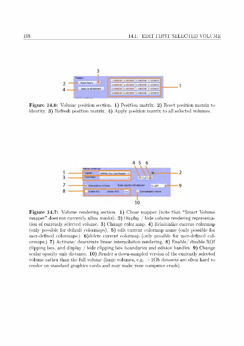
168 14.1. EDIT FIRST SELECTED VOLUME
Figure 14.6: Volume position section. 1) Position matrix. 2) Reset position matrix toidentity. 3) Refresh position matrix. 4) Apply position matrix to all selected volumes.
Figure 14.7: Volume rendering section. 1) Chose mapper (note that "Smart Volumemapper" does not currently allow masks). 2) Display / hide volume rendering representa-tion of currently selected volume. 3) Change color map. 4) Reinitialize current colormap(only possible for default colormaps). 5) edit current colormap name (only possible foruser-de�ned colormaps.) 6)delete current colormap (only possible for user-de�ned col-ormaps.) 7) Activate/ deactivate linear interpolation rendering. 8) Enable/ disable ROIclipping box, and display / hide clipping box boundaries and edition handles. 9) Changescalar opacity unit distance. 10) Render a down-sampled version of the currently selectedvolume rather than the full volume (large volumes, e.g. > 1Gb datasets are often hard torender on standard graphics cards and may make your computer crash).

CHAPTER 14. MENU VOLUMES 169
Figure 14.8: Colormaps. Left: Volume rendering using the rainbow colormap. Center:Volume rendering using the Black-red-white colormap. Right:Volume rendering usingalso the Black-red-white colormap, after the mapped min and mapped max values havebeen shifted.
14.1.6 Volume rendering mask
Volume rendering masking tools are located in this section (see Fig. 14.12 p. 171). Notethat when the Smart Volume Mapper is selected, masking tools become unavailable. Di�erentexamples are provided:Masking using the pencil tool is presented Fig. 14.13 p.172Masking using the lasso is presented Fig.14.14 p.173Masking using the rubber band (rectangular selection) is presented Fig.14.15 p. 173Masking using a 3D surface (in this example: a spherical surface) is presented Fig.14.16 p.174Mask inversion is presented Fig.14.17 p. 175Mask hardening is presented Fig.14.18 p. 176
14.1.7 Color map edition
Volume rendering color map edition controls tools are located in this section (see Fig. 14.19 p.177).
How shifting min and max display range a�ects volume rendering representations is illus-trated Fig. 14.8 p. 169.
14.1.8 Suggested mapped values
You may decide to reset min and max of the color map based on suggested values. Thesesuggested min and max values are computed in order to remove a percentage of most extreme

170 14.1. EDIT FIRST SELECTED VOLUME
Figure 14.9: Scalar Opacity Unit Distance (SOUD) dramatically a�ects volume ren-dering representations. For a given volume, MorphoDig initializes this parameter as afraction of the length of diagonal of the bounding box. However, as illustrated here, youmay decide to adjust SOUD manually.
Figure 14.10: 2D slices 1) Display / hide 2D slices in xy, xz and yz planes. 2) Changeslice number in xy, xz and yz planes.

CHAPTER 14. MENU VOLUMES 171
Figure 14.11: 2D slices representation. Left: by default, the volume rendering rep-resentation is activated, and hides very much the 2D slices. Left: hiding the volumerendering representation improves the visibilty of the 2D slices.
Figure 14.12: Volume rendering mask. 1) Enable/disable mask tools. 2) When usingthe pencil tool, choose between spherical shape and cylindric shape. 3) De�ne pencilradius in terms of screen pixels. Pencil radius can be interactively changed by keeping"T" pressed while rolling the middle mouse button. 4) De�ne whether voxels layinginside the selection should be masked or unmasked. 5) De�ne whether selected voxels tomask/unmask laying inside or outside the selected region. 6) Pencil selection tool. 7)Lasso selection tool. 8) Rectangular region selection tool. 9) 3D surface selection tool:use a 3D surface to de�ne which region should be masked. 10) Reinitialize mask. 11)Invert mask. 12) Harden transform mask. 13) Import mask. 14) Export mask.
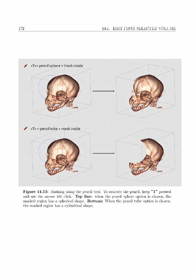
172 14.1. EDIT FIRST SELECTED VOLUME
Figure 14.13: Masking using the pencil tool. To activate the pencil, keep "T" pressedand use the mouse left click. Top line: when the pencil sphere option is chosen, themasked region has a spherical shape. Bottom: When the pencil tube option is chosen,the masked region has a cylindrical shape.
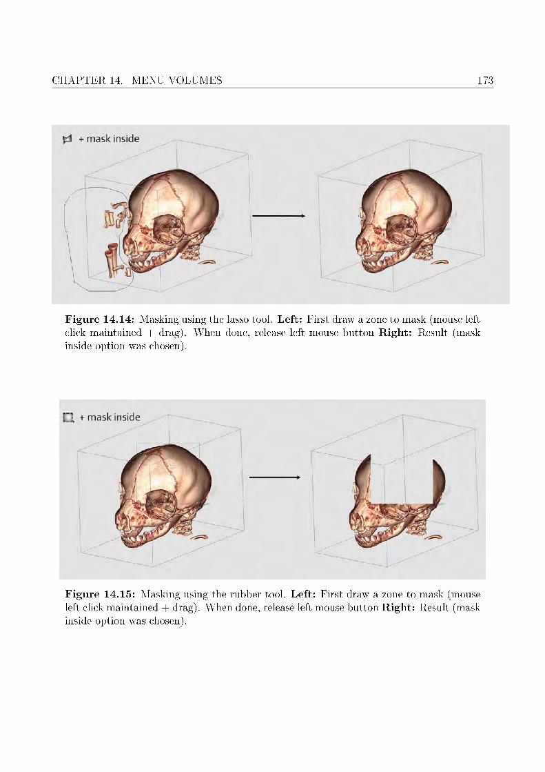
CHAPTER 14. MENU VOLUMES 173
Figure 14.14: Masking using the lasso tool. Left: First draw a zone to mask (mouse leftclick maintained + drag). When done, release left mouse button Right: Result (maskinside option was chosen).
Figure 14.15: Masking using the rubber tool. Left: First draw a zone to mask (mouseleft click maintained + drag). When done, release left mouse button Right: Result (maskinside option was chosen).

174 14.1. EDIT FIRST SELECTED VOLUME
Figure 14.16: Masking using a spherical surface. Top line: mask inside the regionde�ned by the outise of the sphere. Bottom line: mask inside the region de�ned by theinside of the sphere.

CHAPTER 14. MENU VOLUMES 175
Figure 14.17: Mask inversion. Left Volume rendering of the full dataset. MiddleSeveral regions were masked using di�erent masking tools. Right All regions that werehidden are visible, and all regions that were visible are now masked.
minimal and maximal values found in the voxels of the currently opened volume (see Fig. 14.20p. 177).
14.2 Extract isosurface from �rst selected volume
This option opens the "Isosurface" dialog (see Fig. 14.21 p.178). A surface will be producedusing the user-de�ned threshold value given.
An example of isosurface extraction out of 3D volume data is provided Fig. 14.22 p.178.
14.3 Flip or swap �rst selected volume
This option opens the "Flip or Swap exes" dialog (see Fig. 14.23 p.179). Flipping any of theaxes will result in the production of a mirror image of the volume (see for instance Fig. 14.24p.179).
14.4 Change voxel size of �rst selected volume (keep di-
mensions, no resampling
This option opens the "Spacing" dialog (see Fig. 14.25 p.180). Changing voxel size will resultin changes in the displayed dimensions of the volume (see for instance Fig. 14.26 p.180).
Note that adjusting voxel size will not a�ect the dimensions (number of voxels in x,y and zdirections) of the volume.

17614.4. CHANGE VOXEL SIZE OF FIRST SELECTED VOLUME (KEEP DIMENSIONS,
NO RESAMPLING
Figure 14.18: Mask harden transform. A) Volume rendering of the full dataset, andVirtual slice. B) Several regions were masked using di�erent masking tools. Note that thevirtual slice remains unchanged, which indicates that the original dataset remains intact.C) All previously masked voxels are now given the same value (in that case: "0"): theoriginal data is now modi�ed.

CHAPTER 14. MENU VOLUMES 177
Figure 14.19: Volume rendering colormap control section. 1) Opacity control points ofthe active color map (move these points to change opacity). 2) Color control points of theactive color map (double click on each point to edit the color). 3) Histogram of currentlyselected volume. Orange: conventional histogram. Blue: logarithmic-scaled histogram.The 2 vertical bars indicate the min and max display range of the colormap. 4) Shiftcolor map display range, or change min and max display range.5) Edit manually mappedmin or max value. Edit manually histogram plotted min or max. 6) From top to down.a: set range to min and max. b: reverse color control points. c: reverse opacity controlpoints. d: Export colormap to �le. e: Save colormap to presets = duplicate current activecolor map and create a new custom color map.
Figure 14.20: Volume rendering suggested mapped values. 1) Suggested minimal value.2) Suggested maximal value. 3) Apply suggested min value. 4) Apply suggested maxvalue.5) Change the percentage of extreme minimal values to compute a new suggestedminimal value. 6) Change the percentage of extreme maximal values to compute a newsuggested maximal value.

17814.4. CHANGE VOXEL SIZE OF FIRST SELECTED VOLUME (KEEP DIMENSIONS,
NO RESAMPLING
Figure 14.21: Isosurface dialog. A threshold value must be provided. You can ei-ther reconstruct the isosurface using the �ying edges algorithem or the marching cubesalgorithm.
Figure 14.22: Isosurface extraction example. Left: volume rendering representation ofthe cranium of a newborn Lemur catta. Right: 3D isosurface (threshold: 12000).

CHAPTER 14. MENU VOLUMES 179
Figure 14.23: Flip or Swap axes dialog. You may decide either to �ip an axis, or toswap 2 or 3 axes.
Figure 14.24: Example of axis Y �ipping. Left: volume rendering representation of thecranium of a newborn Lemur catta. Right: the same volume rendering representationafter axis Y was �ipped.

18014.4. CHANGE VOXEL SIZE OF FIRST SELECTED VOLUME (KEEP DIMENSIONS,
NO RESAMPLING
Figure 14.25: Edit spacing (voxel size). You may decide to change voxel size in x, y orz dimension.
Figure 14.26: Example of voxel size modi�cation. Left: volume rendering represen-tation of the cranium of a newborn Lemur catta. Right: the same volume renderingrepresentation after axis voxel sized was multiplied by a factor of 2.

CHAPTER 14. MENU VOLUMES 181
Figure 14.27: Resample dialog. Change either voxel size or desired dimensiosn of theoutput volume. Note that voxel size and dimensions are connected.
14.5 Resample �rst selected volume (dimensions will be
changed, and voxel size as well)
This option opens the "Resample" dialog (see Fig. 14.27 p.181). Both voxel size and dimen-sions will be changed, in order that displayed size will be maintained (see for instance Fig.14.28 p.182). The resample dialog is useful when a given dataset is heavy (for instance morethan 1000*1000*1000 voxels), and you want to downsize it to a "reasonable" size (eg. around500*500*500 voxels).
Note that adjusting voxel size will not a�ect the display size in 3D space of the volume.
14.6 Reslice �rst selected volume
This option opens the "Reslice" dialog (see Fig. 14.29 p.183). Rotated volumes will be reslicedalong the desired direction. Note that voxel size will remained untouched, and that the volumerendering representation will stay still as well (see for instance Fig. 14.30 p.184). The reslicedialog is useful when a given specimen was scanned in random orientation, and that you wantto reorient the whole volume.

182 14.6. RESLICE FIRST SELECTED VOLUME
Figure 14.28: Example of volume resampling. Left: volume rendering representation ofthe cranium of a newborn Lemur catta. Right: the same volume rendering representationafter axis voxel sized was multiplied by a factor of 2.

CHAPTER 14. MENU VOLUMES 183
Figure 14.29: Reslice dialog. You can choose among di�erent interpolation methodsto reslice the volume. You may also decide to produce a cropped output or an extendedoutput. The latter option requires more memory, but makes sure that no region of theoriginal volume is lost.
14.7 Median �lter of �rst selected volume
This option opens the "Median Filter" dialog (see Fig. 14.31 p.184). Using a median �lter maybe useful to reduce image noise (see for instance Fig. 14.32 p.185). However using a median�lter will decrease image's sharpness.
14.8 Gaussian �lter of �rst selected volume
This option opens the "Gaussian Filter" dialog (see Fig. 14.33 p.185). Using a gaussian �lteris an alternative ot the median �lter to reduce image noise (see for instance Fig. 14.34 p.185).However using a gaussian �lter will tend decrease image's sharpness very much.
14.9 Invert �rst selected volume
This option inverts the voxel values of the volume (see for instance Fig. 14.35 p.187). In somecases, you may need this option.

184 14.9. INVERT FIRST SELECTED VOLUME
Figure 14.30: Example of volume reslicing. Left: volume rendering representation +2D slices of the cranium of a newborn Lemur catta, which was positioned in a "bilogicallyrelevant" orientation. Right: the same volume rendering representation + 2D slicesafter the whole volume was resliced. Note that the orientaiton the volume renderingrepresentation is maintained.
Figure 14.31: Median �lter dialog. You can choose kernel size along x, y and z axes.
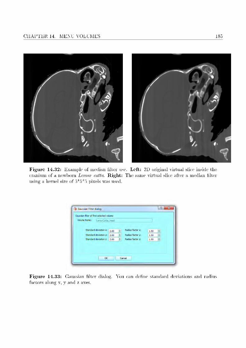
CHAPTER 14. MENU VOLUMES 185
Figure 14.32: Example of median �lter use. Left: 2D original virtual slice inside thecranium of a newborn Lemur catta. Right: The same virtual slice after a median �lterusing a kernel size of 5*5*5 pixels was used.
Figure 14.33: Gaussian �lter dialog. You can de�ne standard deviations and radiusfactors along x, y and z axes.

186 14.9. INVERT FIRST SELECTED VOLUME
Figure 14.34: Example of gaussian �lter use. Left: 2D original virtual slice inside thecranium of a newborn Lemur catta. Right: The same virtual slice after a gaussian �lterwas used (default parameters).

CHAPTER 14. MENU VOLUMES 187
Figure 14.35: Example of voxel values inversion. Left: 2D original virtual slice insidethe cranium of a newborn Lemur catta. Right: The same virtual slice after all voxelvalues were inverted.

188 14.9. INVERT FIRST SELECTED VOLUME

Chapter 15
View
This menu contains the list of widgets which can be viewed or hidden as desired.
189

190

Chapter 16
Help
Contents16.1 MorphoDig Web Site . . . . . . . . . . . . . . . . . . . . . . . . . . . 191
16.2 MorphoDig Tutorials . . . . . . . . . . . . . . . . . . . . . . . . . . . 191
16.3 About... . . . . . . . . . . . . . . . . . . . . . . . . . . . . . . . . . . . 191
16.1 MorphoDig Web Site
This option opens http://morphomuseum.com inside a web navigator.
16.2 MorphoDig Tutorials
This option opens http://www.morphomuseum.com/tutorialsMorphoDig inside a web navi-gator.
16.3 About...
This window (see Fig. 16.1) shows the current version of MorphoDig.
191

192 16.3. ABOUT...
Figure 16.1: About window.

Chapter 17
Acknowledgments
Contents17.1 Design concepts . . . . . . . . . . . . . . . . . . . . . . . . . . . . . . 193
17.2 Code development . . . . . . . . . . . . . . . . . . . . . . . . . . . . . 193
17.3 Specimens illustrated . . . . . . . . . . . . . . . . . . . . . . . . . . . 193
17.4 3D data acquisition facilities . . . . . . . . . . . . . . . . . . . . . . . 194
17.1 Design concepts
I wish to thank Christoph Zollikofer and Marcia Ponce de León, from whom I borrowed manyof the design concepts implemented in FoRM-IT (Fossil Reconstruction and MorphometryInteractive Toolkit; [Zollikofer and Ponce de León, 1995, 2005]).
17.2 Code development
I wish to thank Stefan Schlager and Léo Botton-Divet for their helpful comments and theircontribution to the cross-platform compatibility of the source code.
17.3 Specimens illustrated
I wish to thank the curators of di�erent institutions for the access to most specimens illus-trated in this document: Nathalie Mémoire from the Musée d'Histoire Naturelle de Bordeaux,Christoph Zollikofer and Marcia Ponce de León from the Anthropological Institute and Mu-seum of Zürich, Suzane Jiquel from the ISEM. Thanks also to Mona Le Luyer and PaulineColombet (PACEA, Bordeaux), the PEPS IdEx Bordeaux / CNRS 3 Dent'in for the access to
193

194 17.4. 3D DATA ACQUISITION FACILITIES
the digital reconstruction of the specimen SP07 of Sains-en-Gohelle, and Cédric Beauval andArchéosphère SARL (Bordeaux) for the access to these remains. Thanks to Lionel Hautier andMark Wright for the access to the 3D model of nasal turbinates of Orycteropus afer
17.4 3D data acquisition facilities
I wish to thank the MRI Platform (Montpellier), Zollikofer and Marcia Ponce de León fromthe Anthropological Institute and Museum (Zürich), Paul Ta�oreau and the E.S.R.F. (Greno-ble, France) for the access to the scanning facilities in which the illustrated specimens weredigitized.

References
Lisa S Avila, Sébastien Barré, Rustuy Blue, Diavid Cole, Berk Geveci, William A Ho�man,Brad King, C Chalres Law, Kenneth M Martin, William J Schroeder, and Amy H Squillacote.The VTK User's Guide. 2001. ISBN 1930934238. URL www.vtk.org.
Renaud Lebrun. MorphoDig, 2018. URL http://morphomuseum.com/morphodig.
Christoph P E Zollikofer and Marcia S. Ponce de León. Tools for rapid prototyping in thebiosciences. IEEE Computer Graphics and Applications, 15(6):48�55, 1995. ISSN 02721716.doi: 10.1109/38.469515.
Christoph P E Zollikofer and Marcia S Ponce de León. Virtual Reconstruction: A Primer in
Computer-Assisted Paleontology and Biomedicine. Wiley, New York, 2005. ISBN 978-0-471-20507-4.
195