more “normal” than normal: scaling distributions in complex systems

More “normal” than Normal:Scaling distributions in complex

systems

Walter Willinger (AT&T Labs-Research)David Alderson (Caltech)John C. Doyle (Caltech)

Lun Li (Caltech)

Winter Simulation Conference 2004

Acknowledgments• Reiko Tanaka (RIKEN, Japan)• Matt Roughan (U. Adelaide, Australia)• Steven Low (Caltech)• Ramesh Govindan (USC)• Neil Spring (U. Maryland)• Stanislav Shalunov (Abilene)• Heather Sherman (CENIC)

AgendaMore “normal” than Normal• Scaling distributions, power laws, heavy

tails• Invariance properties

High Variability in Network Measurements• Case Study: Internet Traffic (HTTP, IP)

– Model Requirement: Internal Consistency– Choice: Pareto vs. Lognormal

• Case Study: Internet Topology (Router-level)– Model Requirement: Resilience to

Ambiguity– Choice: Scale-Free vs. HOT

20th Century’s 100 largest disasters worldwide

10-2

10-1

100

100

101

102

US Power outages (10M of customers)

Natural ($100B)

Technological ($10B)

Log(size)

Log(rank)

10-2

10-1

100

100

101

102

Log(Cumulative frequency)

Log(size)

= Log(rank)

Note: it is helpful to use cumulative distributions to avoid statistics mistakes

100

101

102

1

2

3

10

100

10-2

10-1

100

Log(size)

Log(rank)

100

101

102

Median

10-2

10-1

100

Log(size)

Log(rank)

Typical events are relatively small

Largest events are huge (by orders of magnitude)

100

101

102


US Power outages (10M of customers,1985-1997)

Natural ($100B)

Technological ($10B)

Slope = -1

10-2

10-1

100

100

101

102


Slope = -1(=1)

10-2

10-1

100

A random variable X is said to follow a power law with index > 0 if

? 10

0

101

102 US Power outages

(10M of customers, 1985-1997)

10-2

10-1

100

Slope = -1(=1)

A large event is not inconsistent with statistics.

Observed power law relationships

• Species within plant genera (Yule 1925)• Mutants in bacterial populations (Luria and

Delbrück 1943)• Economics: income distributions, city populations

(Simon 1955)• Linguistics: word frequencies (Mandelbrot 1997)• Forest fires (Malamud et al. 1998)• Internet traffic: flow sizes, file sizes, web

documents (Crovella and Bestavros 1997)• Internet topology: node degrees in physical and

virtual graphs (Faloutsos et al. 1999)• Metabolic networks (Barabasi and Oltavi 2004)

Notation• Nonnegative random variable X• CDF: F(x) = P[ X x ] • Complementary CDF (CCDF): 1 – F(x) = P [ X x ]

NB: Avoid descriptions based on probability density f(x)!

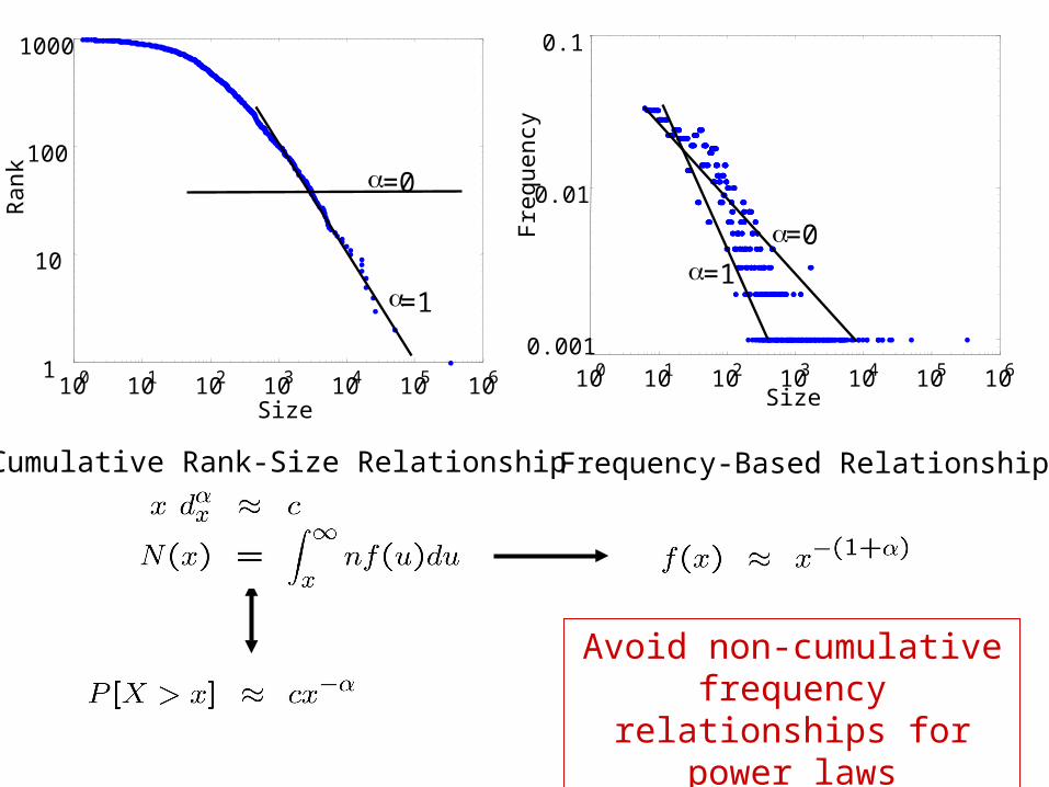
Cumulative Rank-Size Relationship Frequency-Based Relationship


Avoid non-cumulative frequency relationships

for power laws

100 101 102 103 104 105 106Size

0.001

0.01

0.1

Fre

quen

cy

=1

=0

100 101 102 103 104 105 1061

10

100

1000

Size

Ran

k

=1

=0




Avoid non-cumulative frequency relationships

for power laws



For many commonly used distribution functions• Right tails decrease exponentially fast• All moments exist and are finite• Corresponding variable X exhibits low variability

(i.e. concentrates tightly around its mean)

Subexponential DistributionsFollowing Goldie and Klüppelberg (1998), we

say that F (or X) is subexponential if

where X1, X2, …, Xn are IID non-negative random variables with distribution function F.

This says that Xi is likely to be large iff max (Xi) is large (i.e. there is a non-negligible probability of extremely large values in a subexponential sample).

This implies for subexponential distributions that

(i.e. right tail decays more slowly than any exponential)

Heavy-tailed (Scaling) Distributions

A subexponential distribution function F(x) (or random variable X) is called heavy-tailed or scaling if for some 0 < < 2

for some constant 0 < c < .

Parameter is called the tail index• 1 < < 2 F has finite mean, infinite variance• 0 < < 1 F has infinite mean, infinite variance• In general, all moments of order are

infinite.

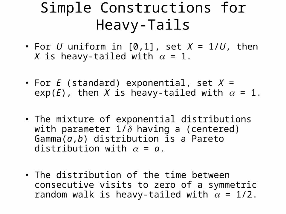
Simple Constructions for Heavy-Tails

• For U uniform in [0,1], set X = 1/U, then X is heavy-tailed with = 1.

• For E (standard) exponential, set X = exp(E), then X is heavy-tailed with = 1.

• The mixture of exponential distributions with parameter 1/ having a (centered) Gamma(a,b) distribution is a Pareto distribution with = a.

• The distribution of the time between consecutive visits to zero of a symmetric random walk is heavy-tailed with = 1/2.

Power Laws

Note that (1) implies

• Scaling distributions are also called power law distributions.• We will use notions of power laws, scaling distributions, and

heavy tails interchangeably, requiring only that

In other words, the CCDF when plotted on log-log scale follows an approximate straight line with slope -.

100

101

102


Slope = -1(=1)

10-2

10-1

100

Why “Heavy Tails” Matter …• Risk modeling (insurance)• Load balancing (CPU, network)• Job scheduling (Web server design)• Combinatorial search (Restart methods)• Complex systems studies (SOC vs. HOT)• Understanding the Internet

– Behavior (traffic modeling)– Structure (topology modeling)

Power laws are ubiquitous• High variability phenomena abound in natural

and man made systems• Tremendous attention has been directed at

whether or not such phenomena are evidence of universal properties underlying all complex systems

• Recently, discovering and explaining power law relationships has been a minor industry within the complex systems literature

• We will use the Internet as a case study to examine the what power laws do or don’t have to say about its behavior and structure.

First, we review some basic properties about scaling distributions

Response to Conditioning• If X is heavy-tailed with index , then the

conditional distribution of X given that X > w satisfies

• The non-heavy-tailed exponential distribution has conditional distribution of the form

For large values, x is identical to the unconditional distribution P[ X > x ], except for a change in scale.

The response to conditioning is a change in location, rather than a change in scale.

• For a scaling distribution with parameter , mean residual lifetime is increasing

Mean Residual Lifetime• An important feature that distinguishes heavy-

tailed distributions from non-heavy-tailed counterparts

• For the exponential distribution with parameter , mean residual lifetime is constant

Key Mathematical Properties of Scaling Distributions

• Response to conditioning (change in scale)• Mean residual lifetime (linearly increasing)

Invariance Properties• Invariant under aggregation

– Non-classical CLT and stable laws• (Essentially) invariant under maximization

– Domain of attraction of Frechet distribution• (Essentially) invariant under mixture

– Example: The largest disasters worldwide• Invariant under marginalization

Linear Aggregation: Classical Central Limit Theorem

• A well-known result– X(1), X(2), … independent and identically

distributed random variables with distribution function F (mean < and variance 1)

– S(n) = X(1) + X(2) +…+ X(n) n-th partial sum

• More general formulations are possible• Often-used argument for the ubiquity of the normal

distribution

Linear Aggregation: Non-classical Central Limit Theorem

• A less well-known result– X(1), X(2), … independent and identically

distributed with common distribution function F that is heavy-tailed with 1 < < 2

– S(n) = X(1)+X(2)+…+X(n) n-th partial sum

• The limit distribution is heavy-tailed with index • More general formulations are possible• Gaussian distribution is special case when = 2• Rarely taught in most Stats/Probability courses

Maximization:Maximum Domain of Attraction

• A not so well-known result (extreme-value theory)– X(1), X(2), … independent and identically

distributed with common distribution function F that is heavy-tailed with 1 < < 2

– M(n) = max(X(1), …, X(n)), n-th successive maxima

• G is the Fréchet distribution exp(-x-)• G is heavy-tailed with index

Weighted Mixture• A little known result

– X(1), X(2), … independent random variables having distribution functions Fi that are heavy-tailed with common index 1 < < 2, but possibly different scale coefficients ci

– Consider the weighted mixture W(n) of X(i)’s

– Let pi be the probability that W(n) = X(i), with p1+…+pn=1, then one can show

where cW = pi ci is the weighted average of the separate scale coefficients ci.

• Thus, the weighted mixture of scaling distributions is also scaling with the same tail index, but a different scale coefficient

Multivariate Case: Marginalization

• For a random vector X Rd, if all linear combinations Y = k bk Xk are stable with 1, then X is a stable vector in Rd with index .

• Conversely, if X is an -stable random vector in Rd then any linear combination Y = k bk Xk is an -stable random variable.

• Marginalization– The marginal distribution of a multivariate

heavy-tailed random variable is also heavy tailed

– Consider convex combination denoted by multipliers b = (0, …, 0, 1, 0, …, 0) that projects X onto the kth axis

– All stable laws (including the Gaussian) are invariant under this type of transformation

Invariance PropertiesGaussian

DistributionsScaling

Distributions

Aggregation Yes Yes

Maximization No Yes

Mixture No Yes

Marginalization Yes Yes

• For low variability data, minimal conditions on the distribution of individual constituents (i.e. finite variance) yields classical CLT

• For high variability data, more restrictive assumption (i.e. right tail of the distribution of the individual constituents must decay at a certain rate) yields greater invariance

Scaling: “more normal than Normal”

• Aggregation, mixture, maximization, and marginalization are transformations that occur frequently in natural and engineered systems and are inherently part of many measured observations that are collected about them.

• Invariance properties suggest that the presence of scaling distributions in data obtained from complex natural or engineered systems should be considered the norm rather than the exception.

• Scaling distributions should not require “special” explanations.

Our Perspective• Gaussian distributions as the natural null

hypothesis for low variability data – i.e. when variance estimates exist, are finite,

and converge robustly to their theoretical value as the number of observations increases

• Scaling distributions as natural and parsimonious null hypothesis for high variability data– i.e. when variance estimates tend to be ill-

behaved and converge either very slowly or fail to converge all together as the size of the data set increases

High-Variability in Network Measurements:

Implications for Internet Modeling and Model Validation


Lun Li (Caltech)

Winter Simulation Conference 2004

G.P.E. Box: “All models are wrong, …

• … but some are useful.”– Which ones?– In what sense?

• … but some are less wrong.– Which ones?– In what sense?

• Mandelbrot’s version:– “When exactitude is elusive, it is

better to be approximately right than certifiably wrong.”

What about Internet measurements?

• High-volume data sets– Individual data sets are huge– Huge number of different data sets– Even more and different data in the future

• Rich semantic context of the data– A packet is more than arrival time and size

• Internet is full of “high variability”– Link bandwidth: Kbps – Gbps– File sizes: a few bytes – Mega/Gigabytes– Flows: a few packets – 100,000+ packets– In/out-degree (Web graph): 1 – 100,000+– Delay: Milliseconds – seconds and beyond

On Traditional Internet Modeling• Step 0: Data Analysis

– One or more sets of comparable measurements• Step 1: Model Selection

– Choose parametric family of models/distributions

• Step 2: Parameter Estimation– Take a strictly static view of data

• Step 3: Model Validation– Select “best-fitting” model– Rely on some “goodness-of-fit” criteria/metrics– Rely on some performance comparison

How to deal with “high variability”?– Option 1: High variability = large, but finite

variance– Option 2: High variability = infinite variance

Some Illustrative Examples• Some commonly-used plotting

techniques– Probability density functions (pdf)– Cumulative distribution functions

(CDF)– Complementary CDF (CCDF)

• Different plots emphasize different features– Main body of the distribution vs. tail– Variability vs. concentration– Uni- vs. multi-modal

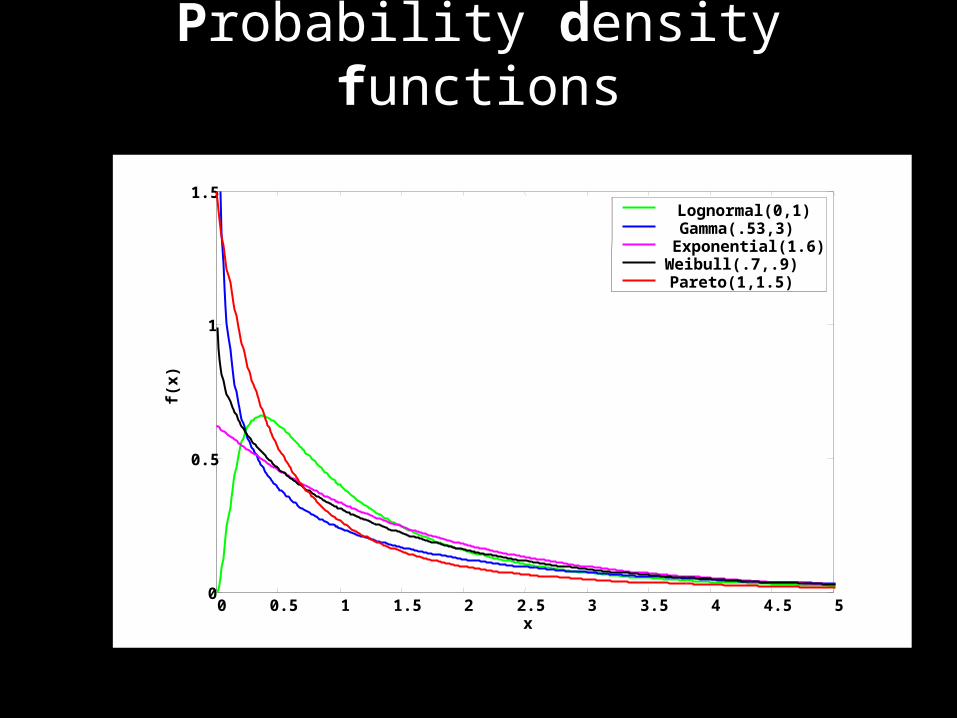
Probability density functions

0 0.5 1 1.5 2 2.5 3 3.5 4 4.5 50

0.5

1

1.5

x

f(x

)

Lognormal(0,1)Gamma(.53,3)Exponential(1.6)

Weibull(.7,.9)Pareto(1,1.5)

Cumulative Distribution Function

0 2 4 6 8 10 12 14 16 18 200

0.1

0.2

0.3

0.4

0.5

0.6

0.7

0.8

0.9

1

x

F(x

)


Weibull(.7,.9)Pareto(1,1.5)

Complementary CDFs

10-1

100

101

102

10-4

10-3

10-2

10-1

100

log(x)

log

(1-F

(x))

Lognormal(0,1)Gamma(.53,3)Exponential(1.6)Weibull(.7,.9)

Complementary CDFs

10-1

100

101

102

10-4

10-3

10-2

10-1

100

log(x)

log

(1-F

(x))


Weibull(.7,.9)ParetoII(1,1.5)ParetoI(0.1,1.5)

By ExampleInternet Traffic• HTTP Connection Sizes from 1996• IP Flow Sizes (2001)

Internet Topology• Router-level connectivity (1996, 2002)

100

102

104

106

108

10-6

10-5

10-4

10-3

10-2

10-1

100

x (HTTP size)

1-F

(x)

HTTP Data

HTTP Connection Sizes (1996)– 1 day of LBL’s WAN traffic (in- and outbound)– About 250,000 HTTP connection sizes (bytes)– Courtesy of Vern Paxson

100

102

104

106

108

10-6

10-5

10-4

10-3

10-2

10-1

100

x (HTTP size)

1-F

(x)

HTTP DataFitted LognormalFitted Pareto

HTTP Connection Sizes (1996)How to deal with “high variability”?

– Option 1: High variability = large, but finite variance

– Option 2: High variability = infinite variance

Fitted2-parameterLognormal(=6.75,=2.05)

Fitted 2-parameter Pareto (=1.27, m=2000)

IP flow

100

105

1010

10-6

10-4

10-2

100

x (IP Flow Size)

1-F

(x)

IP flow data

– 4-day period of traffic at Auckland– About 800,000 IP flow sizes (bytes)– Courtesy of NLANR and Joel Summers

IP Flow Sizes (2001)

IP flow

100

105

1010

10-6

10-4

10-2

100

x (IP Flow Size)

1-F

(x)

IP flow dataFitted LognormalFitted Pareto

How to deal with “high variability”?– Option 1: High variability = large, but finite

variance– Option 2: High variability = infinite variance


100

102

104

106

108

10-6

10-5

10-4

10-3

10-2

10-1

100

x

1-F

(x)

Fitted ParetoSamples fromFitted Pareto

Samples from Pareto Distribution

10-2

100

102

104

106

108

10-6

10-5

10-4

10-3

10-2

10-1

100

x

1-F

(x)

Fitted LognormalSamples fromFitted Lognormal

Samples from Lognormal Distribution

100 102 104 106 10810 -6

10 -5

10 -4

10 -3

10 -2

10 -1

10 0

x

1-F

(x)

Fitted ParetoSamples fromFitted Pareto

10-2 100 102 104 106 10810 -6

10 -5

10 -4

10 -3

10 -2

10 -1

10 0

x

1-F

(x)

Fitted LognormalSamples fromFitted Lognormal

100

102

104

106

108

10-6

10-5

10-4

10-3

10-2

10-1

100

x (HTTP size)

1-F

(x)

HTTP DataFitted LognormalFitted Pareto

100

105

1010

10-6

10-4

10-2

100

x (IP Flow Size)

1-F

(x)


Traditional Modeling Approach• Step 0: Data Analysis• Step 1: Model Selection• Step 2: Parameter Estimation• Step 3: Model Validation

Criticism of Traditional Approach• Highly predictable outcome

– Always doable, no surprises– Cause for endless discussions (Downey’01)

• Curve fitting: when “more” means “better” …– Adding parameters improves fit

• Inadequate “goodness-of-fit” criteria due to– Voluminous data sets– Dependencies, high-variability, non-

stationarities

Beyond Traditional Internet Modeling• Requirement 1: Internal Model Consistency

– Exploit high volume of available data– Learn from Mandelbrot and Tukey– Example: Understanding HTTP and IP data

• Requirement 2: External Model Consistency– Exploit rich semantic of available data– Learn more from Mandelbrot and Cox– Example: Understanding Internet topology data

• Requirement 3: Resilience to Ambiguous Data– High variability to the rescue– Again, look up Mandelbrot!

• Take dynamic view of data– Rely on traditional modeling approach for

initial (small) subset of available data (model M(0))

– Consider successively larger subsets (models M(k))

– Analyze resulting family of models M(0),…,M(n)• Approach: Tukey’s “borrowing strength” idea

– Borrowing strength from large data sets– Simple way to exploit high-volume data sets– Traditional modeling as a means, not as an

end in itself• Internally consistent family of models

– Parameter estimates converge quickly/robustly– 95% Confidence intervals become nested

• Internally inconsistent family of models– Parameter estimates don’t converge– 95% CI’s don’t overlap

Internal Model Consistency

• Lognormal model assumes finite variance• Tool: Mandelbrot’s “sequential moment plots”

– Plot moment estimates as a function of n (sample size)

– Plot corresponding 95% CI as a function of n

– Look for convergence/divergence as n approaches the full sample size

• Practical implementation– Working with raw data– Working with transformations of raw data– Working with random permutation of

transformations of raw data

HTTP Data: Lognormal Family of Models

0 0.5 1 1.5 2 2.5

x 105

0

2

4

6

8

10x 10

4

n (Number of Observations)

ST

D(n

)

HTTP data (original)

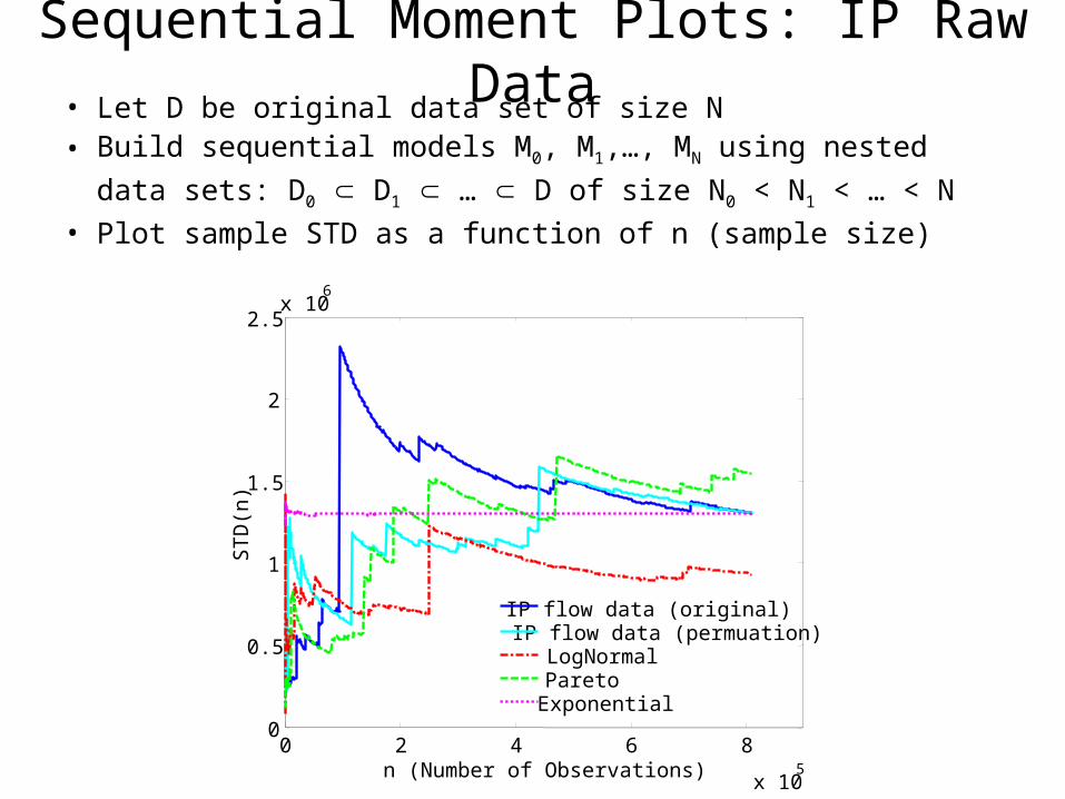
• Let D be original data set of size N• Build sequential models M0, M1,…, MN using nested

data sets: D0 D1 … D of size N0 < N1 < … < N• Plot sample STD as a function of n (sample size)

Sequential Moment Plots: HTTP Raw Data

0 0.5 1 1.5 2 2.5

x 105

0

2

4

6

8

10x 10

4


ST

D(n

)

HTTP data (original)HTTP data (permuation)

Sequential Moment Plots: HTTP Raw Data• Let D be original data set of size N

• Build sequential models M0, M1,…, MN using nested

data sets: D0 D1 … D of size N0 < N1 < … < N• Plot sample STD as a function of n

0 0.5 1 1.5 2 2.5

x 105

0

2

4

6

8

10x 10

4


ST

D(n

)

HTTP data (original)HTTP data (permuation)LogNormal




0 0.5 1 1.5 2 2.5

x 105

0

2

4

6

8

10x 10

4


ST

D(n

)

HTTP data (original)HTTP data (permuation)LogNormalPareto




0 0.5 1 1.5 2 2.5

x 105

0

2

4

6

8

10x 10

4


ST

D(n

)

HTTP data (original)HTTP data (permuation)LogNormalParetoExponential




2.15


0 0.5 1 1.5 2 2.5

x 105

2.1

2.2

2.25

2.3

2.35

2.4

2.45

2.5

2.55

2.6

(n)

^

(n) Estimate^95% CI

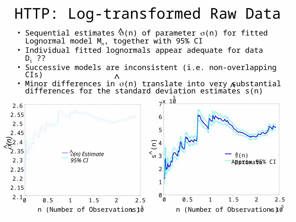
HTTP: Log-transformed Raw Data• Sequential estimates (n) of parameter (n) for fitted

Lognormal model Mn, together with 95% CI• Individual fitted lognormals appear adequate for data D i ??• Successive models are inconsistent (i.e. non-overlapping

CIs)• Minor differences in (n) translate into very substantial

differences for the standard deviation estimates s(n)

s (n

)^

0 0.5 1 1.5 2 2.5

x 105

0

1

2

3

4

5

6

7 x 105


s(n) EstimateApprox 95% CI^

^

^^

Random permutation of log-transformed

raw data

HTTP: Permuted & Transformed Raw Data


0 0.5 1 1.5 2 2.5

x 105

2.1

2.15

2.2

2.25

2.3

2.35

2.4

2.45

2.5

2.55

2.6

(n)

^

(n) Estimate^95% CI

0 0.5 1 1.5 2 2.5

x 105

2.35

2.4

2.45

2.5

2.55

2.6

n (Number of Observation)

(n)

^

Log-transformed raw data

• Question: Are the jumps in the estimate of (n) the result of dependencies in the data?

• Answer: Data permutation gives the appearance of convergence

0 2 4 6 8 10 12 14 16

0.0010.003

0.01 0.02

0.05

0.10

0.25

0.50

0.75

0.90

0.95

0.98 0.99

0.9970.999

Data

Pro

ba

bili

tyNormal Probability Plot

HTTP: Does the log-transformed data fit a normal?

Modeling HTTP DataLognormal models:• Raw data

– Shows lack of convergence of 2nd moment estimates

• Transformed data– Shows impact of dependencies in the data

• Transformed and permuted data– Lognormal model is internally inconsistent

Example of being “certifiably wrong”

HTTP Data: Pareto Family of Models

• Pareto model assumes infinite variance, but is defined in terms of tail index

• Tool: “Sequential tail index estimate plots”– Plot tail index estimates as a function of

n– Plot corresponding 95% CI as a function

of n– Look for convergence/divergence as n

approaches the full sample size• Practical implementation

– Working with raw data– Working with random permutation of

raw data

Random permutation of raw data

HTTP: Sequential Tail Index Estimate Plots

Raw Data

0 0.5 1 1.5 2 2.5x 105

0.8

0.9

1

1.1

1.2

1.3

1.4

1.5

1.6

1.7

1.8


(n) Estimate^95% CI

(

n)^

(n)

0 0.5 1 1.5 2 2.5x 10

5

1

1.1

1.2

1.3

1.4

1.5

1.6

1.7

1.8

1.9

n (Number of Observation)

(n) Estimate^95% CI

^

• Sequential estimates (n) of parameter (n) for fitted Pareto model Mn, together with 95% CI

• Successive fitted Paretos appear largely consistent with one another (i.e. overlapping CIs)

^

0 2 4 6 8 10 12 14 16 18-5

0

5

10

15

20

X Quantiles

Y Q

ua

ntil

es

HTTP: Does the data fit a Pareto?

Pareto Family of Models:• Raw data

– Moment estimates are problematic– Tail index estimates converge quickly

• Permutation of raw data– Tail index estimates converge robustly

(irrespective of dependencies in the data)– Pareto models are internally consistent

Modeling HTTP DataLognormal models:• Raw data




Example of being “approximately right”


0 2 4 6 8 10 12 14 16 18-5

0

5

10

15

20

X Quantiles

Y Q

uan

tile

s

0 2 4 6 8 10 12 14 16

0.0010.0030.01 0.02 0.05 0.10 0.25

0.50

0.75 0.90 0.95 0.98 0.99 0.9970.999

Data

Pro

bab

ility

“All models are wrong… “but some are less wrong.

HTTP: Fitted Lognormal

HTTP: Fitted Pareto

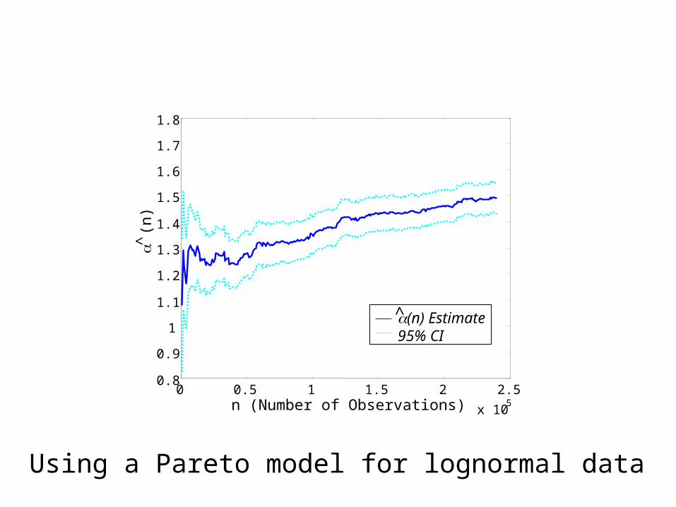
Some Sanity Checks• Fitting Pareto model to Lognormal

sample– Generate iid sample from a

Lognormal model– Check sequential tail index estimate

plot

0 0.5 1 1.5 2 2.5

x 105

0.8

0.9

1

1.1

1.2

1.3

1.4

1.5

1.6

1.7

1.8

(

n)^


(n) Estimate^95% CI

Using a Pareto model for lognormal data

Some Sanity Checks• Fitting Pareto model to Lognormal sample

– Generate iid sample from a Lognormal model– Check sequential tail index estimate plot

• Result: sequential tail index estimates diverge

• Fitting Lognormal model to Pareto sample– Generate iid sample from a Pareto model– Check sequential standard deviation plot– Check normal probability plot

-2 -1 0 1 2 3 4 5 6 7

0.0010.003

0.01 0.02

0.05 0.10

0.25

0.50

0.75

0.90 0.95

0.98 0.99

0.9970.999

Data

Pro

bab

ility

Normal Probability Plot

Using a lognormal model for Pareto data

Some Sanity Checks• Fitting Pareto model to Lognormal sample

– Generate iid sample from a Lognormal model

– Check sequential tail index estimate plot• Result: sequential tail index estimates diverge

• Fitting Lognormal model to Pareto sample– Generate iid sample from a Pareto model– Check sequential standard deviation plot– Check normal probability plot

• Result: transformed data is not Gaussian

IP flow

100

105

1010

10-6

10-4

10-2

100

x (IP Flow Size)

1-F

(x)

IP flow data

– 4-day period of traffic at Auckland– About 800,000 IP flow sizes (bytes)– Courtesy of NLANR and Joel Summers


IP flow

100

105

1010

10-6

10-4

10-2

100

x (IP Flow Size)

1-F

(x)


Finite Variance vs Infinite Variance?

– Sequential moment plots: IP raw data– Sequential estimates of (n): log-transformed

raw data– Sequential tail index plots: estimates of (n)



Sequential Moment Plots: IP Raw Data

IP flow data (original)

0 2 4 6 8

x 105

0

0.5

1

1.5

2

2.5x 10

6


ST

D(n

)




IP flow data (original)IP flow data (permuation)

0 2 4 6 8

x 105

0

0.5

1

1.5

2

2.5x 10

6


ST

D(n

)




IP flow data (original)IP flow data (permuation)LogNormal

0 2 4 6 8

x 105

0

0.5

1

1.5

2

2.5x 10

6


ST

D(n

)




IP flow data (original)IP flow data (permuation)LogNormalPareto

0 2 4 6 8

x 105

0

0.5

1

1.5

2

2.5x 10

6


ST

D(n

)




IP flow data (original)IP flow data (permuation)LogNormalParetoExponential

0 2 4 6 8

x 105

0

0.5

1

1.5

2

2.5x 10

6


ST

D(n

)

• Sequential estimates (n) of parameter (n) for fitted Lognormal model Mn, together with 95% CI

• Individual fitted lognormals appear adequate for data Di,but successive models are inconsistent (i.e. non-overlapping CIs)

• Minor differences in (n) translate into very substantial differences for the standard deviation estimates s(n)

0 1 2 3 4 5 6 7 8 9x 10

5

1.85

1.9

1.95

2

2.05

2.1

2.15

2.2

2.25


(n)

^

(n) Estimate^95% CI

0 1 2 3 4 5 6 7 8 9x 105

1

2

3

4

5

6

7x 105


s (n

)

s(n) EstimateApprox 95% CI

^

^

IP: Log-transformed Raw Data^

^^

(

n)^


(n) Estimate^95% CI

0 1 2 3 4 5 6 7 8 9

x 105

0.4

0.5

0.6

0.7

0.8

0.9

1

1.1

1.2

1.3

1.4

IP Data: Sequential Tail Index Estimate Plots

• Sequential estimates (n) of parameter (n) for fitted Pareto model Mn, together with 95% CI

• Successive fitted Paretos appear largely consistent with one another (i.e. overlapping CIs)

^

Pareto Family of Models:• Raw data

– Moment estimates are problematic– Tail index estimates converge quickly

• Permutation of raw data– Tail index estimates converge robustly

(irrespective of dependencies in the data)– Pareto models are internally consistent

Modeling HTTP and IP DataLognormal models:• Raw data




Example of being “approximately right”




• Requirement 2: External Model Consistency– Exploit rich semantic of available data– Learn more from Mandelbrot and Cox– Example: Understanding self-similar Internet

traffic

• Requirement 3: Resilience to Ambiguous Data– High variability to the rescue– Again, look up Mandelbrot– Example: Understanding Internet topology data

Internet Traffic: Poisson Models• Internally inconsistent

– Earlier criterion applied to processes– D. Figueiredo et al. (2004)

• Externally inconsistent– Aggregate Poisson is incompatible

with high variability of the higher-layer constituents

• Example of being “verifiably wrong”

Internet Traffic: Self-Similar Models• Internally consistent

– Earlier criterion applied to processes– D. Figueiredo et al. (2004)

• Externally consistent– Mandelbrot/Cox construction– LRD via high variability of the higher-

layer constituents– Optimal web layout: heavy-tailed

HTTP data• Example of being “approximately right”

Models of Self-Similar TrafficMandelbrot’s Construction• Renewal reward processes and their aggregates

– Aggregate is made up of many constituents– Each constituent is of the on/off type– On/off periods have a “duration” – Constituents make contributions (“rewards”) when

“on”– Constituents make no contributions when “off”

Cox’s construction• Known as immigration-death or M/G/ process

– Aggregate traffic is made up of many connections– Connections arrive at random– Each connection has a “size” (number of packets)– Each connection transmits packets at some “rate”

• The limiting regimes for the aggregate are essentially the same as those for Mandelbrot’s construction

External Model Consistency

• Cross-layer view of models– Aggregate link traffic (packet-level)– Semantic context in packet trace data allows for

identification of higher-layer constituents [IP flow, TCP connections, HTTP requests/responses, etc.]

– Aggregate link traffic (higher-layer constituents)

• External model consistency– Models respect layered network architecture– Models are required to be consistent across layers– Models explain observed phenomena at different

layers

-6 -5 -4 -3 -2 -1 0 1 2-1

0

1

2

3

4

5

6

Size of events

Frequency

Decimated dataLog (base 10)

Forest fires1000 km2

(Malamud)

WWW filesMbytes

(Crovella)

Data compression

(Huffman)

Cumulative

-6 -5 -4 -3 -2 -1 0 1 2-1

0

1

2

3

4

5

6

Size of events

FrequencyFires

Web filesCodewords

Cumulative

Log (base 10)

-1/2

-1

-6 -5 -4 -3 -2 -1 0 1 2-1

0

1

2

3

4

5

6

Size of events


WWW filesMbytes

Data compression

-1/2

-1 Files

FiresMostfilesare

smallMost packetsare in a fewlarge files

Mice

Elephants

-6 -5 -4 -3 -2 -1 0 1 2-1

0

1

2

3

4

5

6

Size of events


WWW filesMbytes

Data compression

-1/2

-1

Mice

Elephants

Files

Fires

Mice

Elephants

Delay sensitive

Bandwidth sensitive

Probability of user access

Generalized “coding” theoryShannon• Minimize avg file

transfer• No feedback• Discrete (0-d)

topology

Web layout• Minimize avg file

transfer• Feedback• 1-d topology

Web

Data compression

Reference: Zhu, X., J. Yu, and J.C. Doyle. Heavy Tails,Generalized Coding, and Optimal Web Layout. Proceedings of the IEEE Infocom 2001.

-6 -5 -4 -3 -2 -1 0 1 2-1

0

1

2

3

4

5

6

WWWDC

Data

-6 -5 -4 -3 -2 -1 0 1 2-1

0

1

2

3

4

5

6

WWWDC

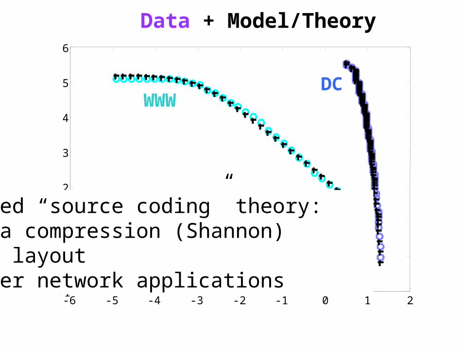
Data + Model/Theory

-6 -5 -4 -3 -2 -1 0 1 2-1

0

1

2

3

4

5

6

WWWDC

Data + Model/Theory

Unified “source coding” theory:1. Data compression (Shannon)2. Web layout3. Other network applications

How general is this mice/elephant picture?

• Selecting and reading books• Selecting and reading magazine articles• Selecting and viewing television• Deciding what movie to go to• Deciding where to go on vacation• Deciding which meetings and classes to

attend• Etc….

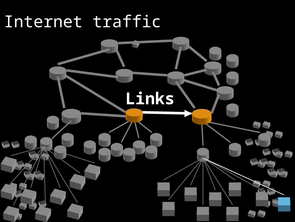
Links

Internet traffic

Typical web traffic

log(file size)

> 1.0log(freq > size)

p s-

Web servers

Heavy tailed web traffic

Is streamed out on the net.

Creating fractal Gaussian internet traffic (Willinger,…)

2

3 H

Fat tail web traffic

Is streamed onto the Internet

creating long-range correlations with 2

3 H

time

Typical web traffic

log(file size)

> 1.0log(freq > size)

p s-

Web servers

Heavy tailed web traffic

Is streamed out on the net.

Externally consistent, rigorous theory with

supporting measurements

2

3 H

The “Closing the Loop” Approach 1. Discovery (data-driven)2. Modeling, subject to internal and external

consistency3. Proposed explanation in terms of elementary

concepts or mechanisms (mathematics)4. Step 3 suggests first-of-its-kind measurements or

revisiting existing measurements related to checking the elementary concepts or mechanisms

5. Empirical validation of elementary concepts or mechanisms using the data collected in Step 4

Why “Closing the Loop” is Progress• Departure from classical “data-fitting”• Validation is moved to a more elementary or

fundamental level• Fully exploits the context in which measurements

are made (“start with data, end with data”)• If successful, provides actual explanation of

“emergent” phenomena (new insight)• Shows inherent limitations and weaknesses of

proposed model, suggests further improvements

100

102

104

106

10810

-6

10-5

10-4

10-3

10-2

10-1

100

x (HTTP size)

1-F

(x)

HTTP Data

Modeling Internet Traffic– More than “curve fitting”– More than “follows a power law”– Fully consistent with theory and empirical

evidence– Validated by “closing the loop”

100

105

1010

10-6

10-4

10-2

100

x (IP Flow Size)

1-F

(x)

IP flow data



• Requirement 2: External Model Consistency– Exploit rich semantic of available data– Learn more from Mandelbrot and Cox– Example: Understanding self-similar Internet

traffic

• Requirement 3: Resilience to Ambiguous Data– High variability to the rescue– Again, look up Mandelbrot– Example: Understanding Internet topology data

Internet Topology

• Internet router-level topology– Physical connectivity– Direct inspection generally not possible

• Available measurements: Traceroute-based– Pansiot and Grad (1998)– Rocketfuel data (Spring et al. 2002)– A few accurate router-level maps

• Other models: AS graphs, WWW graphs

What does the structure of the Internet look like?

Router-Level Topology

Hosts

Routers

• Nodes are machines (routers or hosts) running IP protocol

• Measurements taken from traceroute experiments that infer topology from traffic sent over network

• Subject to sampling errors and bias

• Requires careful interpretation

AS Topology• Nodes are entire

networks (ASes)• Links = peering

relationships between ASes

• Relationships inferred from Border Gateway Protocol (BGP) information

• Really a measure of business relationships, not network structure

AS1

AS3

AS4

AS2

100

101

10210

0

101

102

103

104

Node Degree

Nod

e R

ank

Pansiot-Grad data (1995) of router-level Internet connectivitybased on large-scale traceroute experiments

Faloutsos et al. (1999): Power law degree distribution

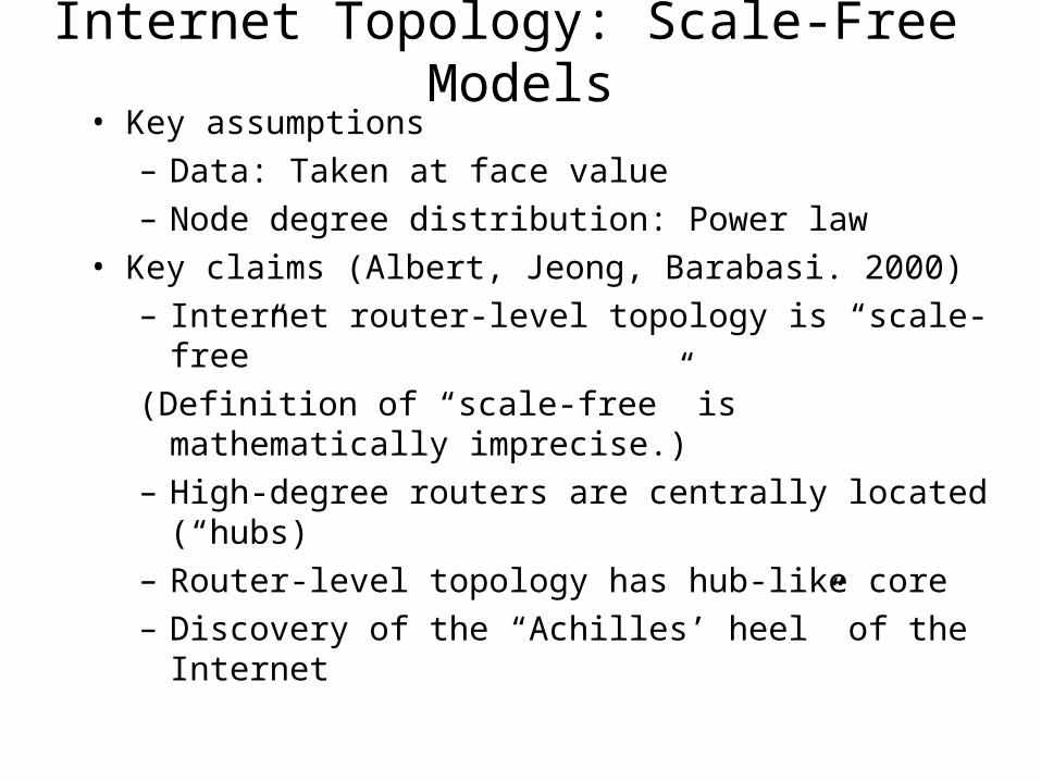
Internet Topology: Scale-Free Models• Key assumptions

– Data: Taken at face value– Node degree distribution: Power law

• Key claims (Albert, Jeong, Barabasi. 2000)– Internet router-level topology is “scale-free”(Definition of “scale-free” is mathematically

imprecise.)– High-degree routers are centrally located

(“hubs)– Router-level topology has hub-like core– Discovery of the “Achilles’ heel” of the Internet

On Resilience to Data Ambiguity• Traceroute-based measurements

– Bias (location of sources)– Incompleteness (number of

destinations)– Errors (alias resolution)– Layer 3 (IP) vs. layer 2 issues

• Inferred node degree distribution– Observed power law may be artifact

of data– Where are the highly-connected

nodes?

Internet Topology: Scale-Free Models

• Exploit semantic context of available data– Core routers have low degrees– High-degree routers at the edge of

the network– Lack of high variability in router-level

core networks

100

101

102

103

100

101

102

103

104

Node Degree

Nod

e R

ank

all nodesr1 nodesr0 nodes

Node degree distribution for AS 7018 (Rocketfuel)

• Nodes categorized by “radius”• “r0” nodes are most “central” (i.e. in the network core)

High variabilityis toward the network edge.

100

101

102

100

101

102

103

Node Degree

Nod

e R

ank

Degree Distribution for AS 7018 - By Router Type

all core routersaccess routersbackbone routers

A closer look at “r0” (core) nodes…

• Access routers: traffic aggregation within each POP• Backbone routers: connectivity between POPs

Model Validation: Scale-Free Models• Exploit semantic context of available data

– Core routers have low degrees– High-degree routers at the edge of the

network– Lack of high variability in router-level core

networks• Scale-free models and Internet topology

– Not resilient to ambiguities in the data– Externally inconsistent (hub nodes in the core)– Ignore all engineering details– Example of being “certifiably wrong”– The Internet is exactly the opposite of what

scale-free models claim in essentially every meaningful aspect

PA PLRG

HOT Abilene-inspired Sub-optimal

Internet Topology: Scale-Rich Models• Key assumption

– Heuristically optimized topology (HOT) design• Approach

– Perspective of individual Internet Service Provider (ISP)

– Consider economic and technological forces at work– Reconcile engineering tradeoffs in design

• Key implications– Mesh-like core of low degree routers– High-degree nodes are at the edge of the network– The Internet “Achilles’ heel” is not connectivity

• Scale-rich models and Internet topology– Resilient to ambiguities in the data– Externally consistent– Example of being “approximately right”

100

101

102

Degree

10-1

100

101

102

103

Ban

dwid

th (

Gbp

s)

15 x 10 GE

15 x 3 x 1 GE

15 x 4 x OC12

15 x 8 FE

Technology constraint

Total Bandwidth

Bandwidth per Degree

Router Technology ConstraintCisco 12416 GSR, circa 2002

high BW low degree high

degree low BW

0.01

0.1

1

10

100

1000

10000

100000

1000000

1 10 100 1000 10000degree

To

tal R

ou

ter

BW

(M

bp

s)

cisco 12416

cisco 12410

cisco 12406

cisco 12404

cisco 7500

cisco 7200

linksys 4-port router

uBR7246 cmts(cable)

cisco 6260 dslam(DSL)

cisco AS5850(dialup)

approximateaggregate

feasible region

Aggregate Router Feasibility

Source: Cisco Product Catalog, June 2002

core technologies

edge technologies

older/cheaper technologies

Heuristically Optimal Topology

Hosts

Edges

Cores

Mesh-like core of fast, low degree routers

High degree nodes are at the edges.

SOX

SFGP/AMPATH

U. Florida

U. So. Florida

Miss StateGigaPoP

WiscREN

SURFNet

Rutgers U.

MANLAN

NorthernCrossroads

Mid-AtlanticCrossroads

Drexel U.

U. Delaware

PSC

NCNI/MCNC

MAGPI

UMD NGIX

DARPABossNet

GEANT

Seattle

Sunnyvale

Los Angeles

Houston

Denver

KansasCity

Indian-apolis

Atlanta

Wash D.C.

Chicago

New York

OARNET

Northern LightsIndiana GigaPoP

MeritU. Louisville

NYSERNet

U. Memphis

Great Plains

OneNetArizona St.

U. Arizona

Qwest Labs

UNM

OregonGigaPoP

Front RangeGigaPoP

Texas Tech

Tulane U.

North TexasGigaPoP

TexasGigaPoP

LaNet

UT Austin

CENIC

UniNet

WIDE

AMES NGIX

PacificNorthwestGigaPoP

U. Hawaii

PacificWave

ESnet

TransPAC/APAN

Iowa St.

Florida A&MUT-SWMed Ctr.

NCSA

MREN

SINet

WPI

StarLight

IntermountainGigaPoP

Abilene BackbonePhysical Connectivity(as of December 16, 2003)

0.1-0.5 Gbps0.5-1.0 Gbps1.0-5.0 Gbps5.0-10.0 Gbps

U.S. Population Density by County1990 Census Data (adjusted 2000)

1

10

100

1000

10000

0.1 10 1000 100000

Population per sq. km.

RA

NK

Rank (number of users)

Con

necti

on

Sp

eed

(M

bp

s)

1e-1

1e-2

1

1e1

1e2

1e3

1e4

1e21 1e4 1e6 1e8

Dial-up~56Kbps

BroadbandCable/DSL~500Kbps

Ethernet10-100Mbps

Ethernet1-10Gbps

most users

have low speed

connections

a few users

have very high

speed connectio

ns

high performancecomputing

academic and corporate

residential and small business

High variability in willingness to

pay for bandwidth by

end users

High variability in population

density

Router-Level Topologies: Rocketfuel

AS Name Routers Links POPs

1221

Telstra (Aus.) 4,440 4,996 54

1239

Sprintlink (US)

11,889 15,263 25

1755

Ebone (EU) 438 1,192 26

2914

Verio (US) 7,574 19,175 103

3257

Tiscali (EU) 618 839 52

3356

Level3 (US) 2,064 8,669 44

3967

Exodus (US) 688 2,166 22

4755

VSNL (India) 664 484 8

6461

Abovenet (US)

843 2,667 22

7018

AT&T (US) 13,993 18,083 109

Neil Spring, Ratul Mahajan, and David Wetherall. Measuring ISP Topologies with Rocketfuel. ACM SIGCOMM 2002.

Validation from ISPs: “good” to “excellent”

External Consistency: Improving Rocketfuel

Approach:• Use additional context specific information to

validate and augment the data collected by Rocketfuel

• Use knowledge about Heuristically Optimal Topology to “reverse-engineer” the structure within an ISP Point of Presence (PoP)

• Unexpected result: node duplicates in large PoPs

AS 7018 9261 total nodes640 core nodes156 duplicates (24%)484 unique core nodes

AS 1239 7043 total nodes673 core nodes215 duplicates (32%)458 unique core nodes

AS 7018: Phoenix, AZ

Lessons LearnedHigh Variability and Scaling Distributions• Don’t be surprised!• Don’t fight high variability when it’s apparent!

– There are ways to check for genuine high variability

• Exploit high variability when it’s there!– Provides basis for explanatory modeling

• Don’t force high variability when it’s absent!– A straight-looking log-log plot is not a proof

Internet Modeling• Need for internal and external consistency• Need for “closing the loop”: empirical validation• Explanatory and not merely descriptive

modeling

Some References• W. Willinger, D Alderson, J.C. Doyle, and L. Li, More “normal”

than Normal: scaling distributions in complex systems. WSC 2004.

• W. Willinger, D Alderson, and L. Li, A pragmatic approach to dealing with high-variability in network measurements, Proc. ACM SIGCOMM IMC 2004, Taormina, Italy

• L. Li, D. Alderson, W. Willinger, and J. Doyle, A first-principles approach to understanding the Internet’s router-level topology, Proc. ACM SIGCOMM 2004, Portland, OR

• D. Figueiredo, B. Liu, A. Feldmann, V. Mishra, D. Towsley, and W. Willinger, On TCP and self-similar traffic, Performance Evaluation (to appear).

• W. Willinger, R. Govindan, S. Jamin, V. Paxson, and S. Shenker, Critically examining criticality: Scaling phenomena in the Internet, PNAS, Vol. 99, 2002.

• Zhu, X., J. Yu, and J.C. Doyle. Heavy Tails, Generalized Coding, and Optimal Web Layout. Proc. of the IEEE Infocom 2001.

More “normal” than Normal:Scaling distributions in complex

systems


Lun Li (Caltech)

[email protected]/~alderd/

topology/

more “normal” than normal: scaling distributions in complex systems

Documents

p x x nb

p x x complementary

finitecorresponding

probability density

cumulative distributions

power law relationshipsspecies

normalscaling distributions

income distributions