www.ck12.org Chapter 4. Normal Distributions

CHAPTER 4 Normal DistributionsChapter Outline

4.1 A LOOK AT NORMAL DISTRIBUTIONS

4.2 STANDARD DEVIATION

4.3 THE EMPIRICAL RULE

4.4 Z-SCORES

71

4.1. A Look at Normal Distributions www.ck12.org

4.1 A Look at Normal Distributions

Learning Objectives

• Identify the characteristics of a normal distribution.• Determine if a variable is normally distributed.

Introduction

Most high schools have a set amount of time in-between classes during which students must get to their next class. Ifyou were to stand at the door of your statistics class and watch the students coming in, think about how the studentswould enter. Usually, one or two students enter early, then more students come in, then a large group of studentsenter, and finally, the number of students entering decreases again, with one or two students barely making it ontime, or perhaps even coming in late!

Now consider this. Have you ever popped popcorn in a microwave? Think about what happens in terms of therate at which the kernels pop. For the first few minutes, nothing happens, and then, after a while, a few kernelsstart popping. This rate increases to the point at which you hear most of the kernels popping, and then it graduallydecreases again until just a kernel or two pops.

Here’s something else to think about. Try measuring the height, shoe size, or the width of the hands of the students inyour class. In most situations, you will probably find that there are a couple of students with very low measurementsand a couple with very high measurements, with the majority of students centered on a particular value.

All of these examples show a typical pattern that seems to be a part of many real-life phenomena. In statistics,because this pattern is so pervasive, it seems to fit to call it normal, or more formally, the normal distribution.

Examples of values that typically follow a normal distribution include:

• Physical characteristics such as height, weight, arm or leg length, etc.• The percentile rankings of standardized testing such as the ACT and SAT• The volume of water produced by a river on a monthly or yearly basis• The velocity of molecules in an ideal gas

The normal distribution is an extremely important concept. It occurs often in the data we collect from the naturalworld, and it is a critical component of many of the more theoretical ideas that are the foundation of statistics. Thischapter explores the details of the normal distribution.

The Characteristics of a Normal Distribution

Shape

When graphing the data from each of the examples in the introduction, the distributions from each of these situationswould be mound-shaped and mostly symmetric. A normal distribution is a perfectly symmetric, mound-shapeddistribution. It is commonly referred to the as a normal curve, or bell curve.

72

www.ck12.org Chapter 4. Normal Distributions

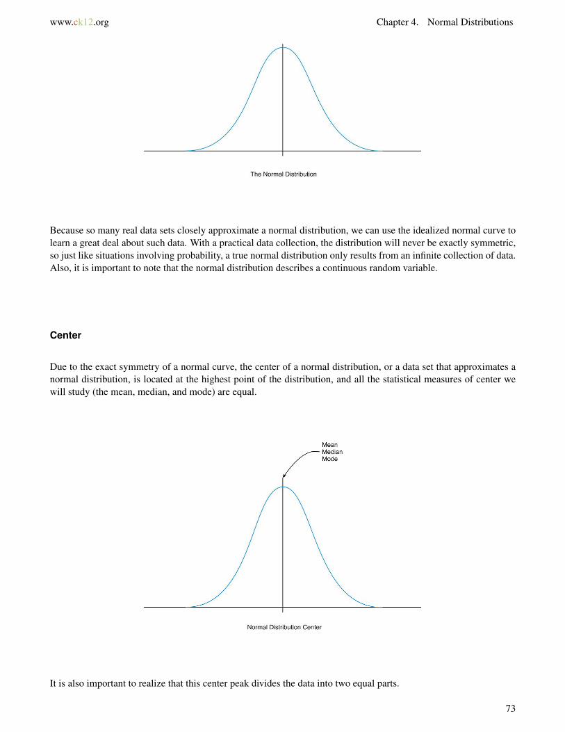
Because so many real data sets closely approximate a normal distribution, we can use the idealized normal curve tolearn a great deal about such data. With a practical data collection, the distribution will never be exactly symmetric,so just like situations involving probability, a true normal distribution only results from an infinite collection of data.Also, it is important to note that the normal distribution describes a continuous random variable.

Center

Due to the exact symmetry of a normal curve, the center of a normal distribution, or a data set that approximates anormal distribution, is located at the highest point of the distribution, and all the statistical measures of center wewill study (the mean, median, and mode) are equal.

It is also important to realize that this center peak divides the data into two equal parts.

73

4.1. A Look at Normal Distributions www.ck12.org

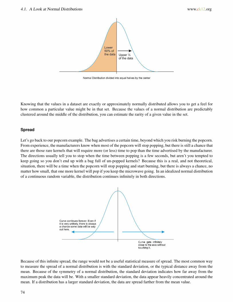
Knowing that the values in a dataset are exactly or approximately normally distributed allows you to get a feel forhow common a particular value might be in that set. Because the values of a normal distribution are predictablyclustered around the middle of the distribution, you can estimate the rarity of a given value in the set.

Spread

Let’s go back to our popcorn example. The bag advertises a certain time, beyond which you risk burning the popcorn.From experience, the manufacturers know when most of the popcorn will stop popping, but there is still a chance thatthere are those rare kernels that will require more (or less) time to pop than the time advertised by the manufacturer.The directions usually tell you to stop when the time between popping is a few seconds, but aren’t you tempted tokeep going so you don’t end up with a bag full of un-popped kernels? Because this is a real, and not theoretical,situation, there will be a time when the popcorn will stop popping and start burning, but there is always a chance, nomatter how small, that one more kernel will pop if you keep the microwave going. In an idealized normal distributionof a continuous random variable, the distribution continues infinitely in both directions.

Because of this infinite spread, the range would not be a useful statistical measure of spread. The most common wayto measure the spread of a normal distribution is with the standard deviation, or the typical distance away from themean. Because of the symmetry of a normal distribution, the standard deviation indicates how far away from themaximum peak the data will be. With a smaller standard deviation, the data appear heavily concentrated around themean. If a distribution has a larger standard deviation, the data are spread farther from the mean value.

74

www.ck12.org Chapter 4. Normal Distributions

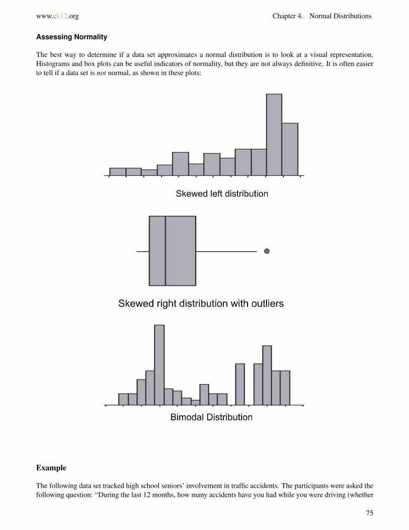
Assessing Normality

The best way to determine if a data set approximates a normal distribution is to look at a visual representation.Histograms and box plots can be useful indicators of normality, but they are not always definitive. It is often easierto tell if a data set is not normal, as shown in these plots:

Example

The following data set tracked high school seniors’ involvement in traffic accidents. The participants were asked thefollowing question: “During the last 12 months, how many accidents have you had while you were driving (whether

75

4.1. A Look at Normal Distributions www.ck12.org

or not you were responsible)?”

TABLE 4.1:

Year Percentage of high school seniors who said theywere involved in no traffic accidents

1991 75.71992 76.91993 76.11994 75.71995 75.31996 74.11997 74.41998 74.41999 75.12000 75.12001 75.52002 75.52003 75.8

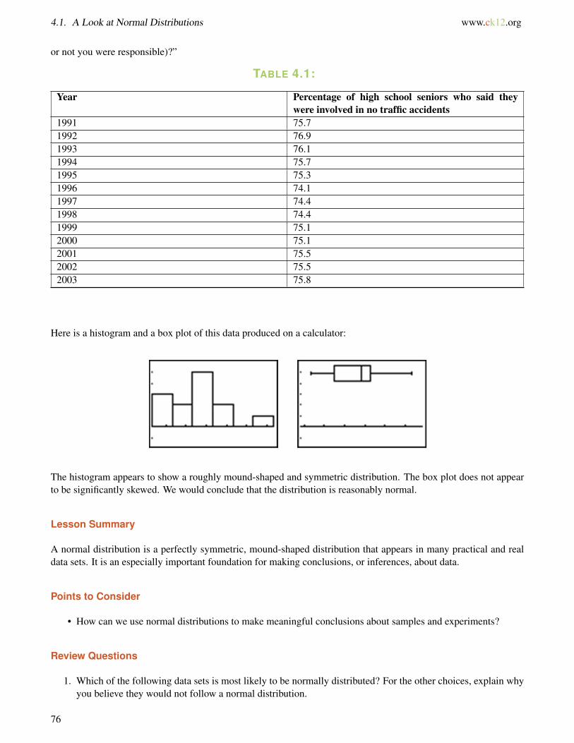
Here is a histogram and a box plot of this data produced on a calculator:

The histogram appears to show a roughly mound-shaped and symmetric distribution. The box plot does not appearto be significantly skewed. We would conclude that the distribution is reasonably normal.

Lesson Summary

A normal distribution is a perfectly symmetric, mound-shaped distribution that appears in many practical and realdata sets. It is an especially important foundation for making conclusions, or inferences, about data.

Points to Consider

• How can we use normal distributions to make meaningful conclusions about samples and experiments?

Review Questions

1. Which of the following data sets is most likely to be normally distributed? For the other choices, explain whyyou believe they would not follow a normal distribution.

76

www.ck12.org Chapter 4. Normal Distributions

(a) The hand span (measured from the tip of the thumb to the tip of the extended 5th finger) of a randomsample of high school seniors

(b) The annual salaries of all employees of a large shipping company

(c) The annual salaries of a random sample of 50 CEOs of major companies, 25 women and 25 men

(d) The dates of 100 pennies taken from a cash drawer in a convenience store

77

4.2. Standard Deviation www.ck12.org

4.2 Standard Deviation

Learning Objectives

• Understand the meaning of standard deviation.• Understanding the percents associated with standard deviation.• Calculate the standard deviation for a normally distributed random variable.

Mean and Standard Deviation

When data is normally or nearly normally distributed, there are two preferred measures of center and spread. Theseare the arithmetic mean and the standard deviation. You are already familiar with the mean. The standard deviationof a data set tells us how it is spread out. The larger the standard deviation is, the more spread out the data is.

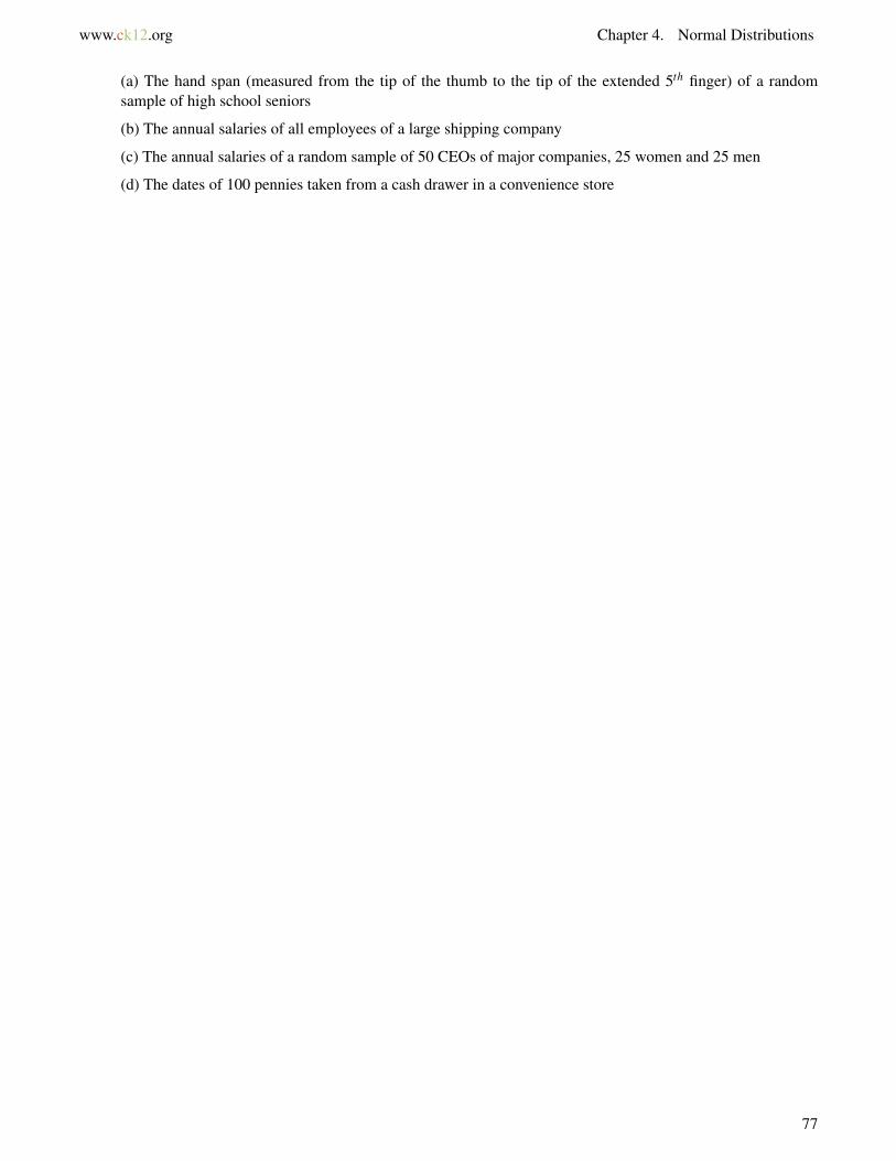
Let’s begin our discussion by visualizing the standard deviation on a normal curve. In a normal distribution, thecurve appears to change its shape from being concave down (looking like an upside-down bowl) to being concave up(looking like a right-side-up bowl). This happens on both sides of the curve, as is shown in the figure below. Wherethis happens is called an inflection point of the curve.

If a vertical line is drawn from an inflection point to the x-axis, you would be marking the location of the score inthe distribution that was one standard deviation from the mean (or the center) of the distribution). For all normaldistributions, approximately 68% of all the data is located within 1 standard deviation of the mean.

If we consider using the unit of standard deviation as a step along the x-axis, then 1 step to the right or 1 step to theleft is considered 1 standard deviation away from the mean. 2 steps to the left or 2 steps to the right are considered 2standard deviations away from the mean. Likewise, 3 steps to the left or 3 steps to the right are considered 3 standarddeviations away from the mean.

The larger the size of that one step, the larger the standard deviation’s numerical value. Hence, in a distributionwhere all the scores are tightly clustered around the mean, the standard deviation is small. When the scores are morespread out, the standard deviation is larger.

78

www.ck12.org Chapter 4. Normal Distributions

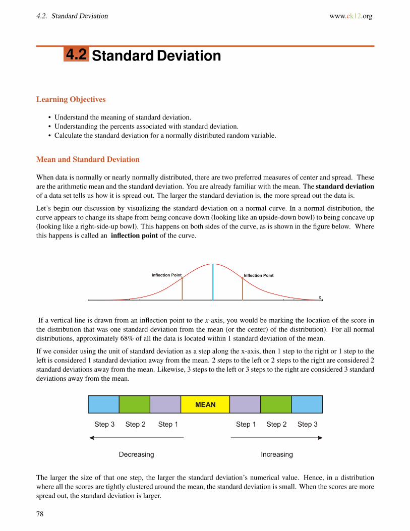
Once the value of the standard deviation has been calculated, you can determine the data value that is exactly one,two or three standard deviations from the mean. For example. if the value of the mean for this distribution was 58,and the value of the standard deviation was 5, then you could identify the values that fall each step away.

Now that you understand the distribution of the data and exactly how it moves away from the mean, you are readyto calculate the standard deviation of a data set. For the calculation steps to be organized, a table is used to recordthe results for each step. The table will consist of 3 columns. The first column will contain the data and will belabeled x. The second column will contain the differences between the data values and the mean of the data set.This column will be labeled (x− x). The final column will be labeled (x− x)2, and it will contain the square of eachof the values recorded in the second column. Note that we are using the symbols for sample statistics, rather thanpopulation parameters.

Example A

Calculate the standard deviation of the following numbers:

2,7,5,6,4,2,6,3,6,9

Solution

• Step 1: Write the list of data values in a column. It is not necessary to organize the data.• Step 2: Calculate the mean of the data values.

x̄ =2+7+5+6+4+2+6+3+6+9

10=

5010

= 5.0

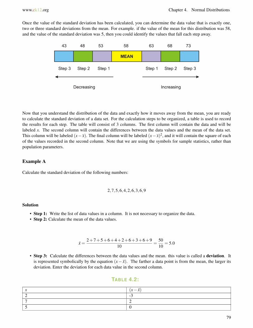
• Step 3: Calculate the differences between the data values and the mean. this value is called a deviation. Itis represented symbolically by the equation (x− x̄). The farther a data point is from the mean, the larger itsdeviation. Enter the deviation for each data value in the second column.

TABLE 4.2:

x (x− x̄)2 -37 25 0

79

4.2. Standard Deviation www.ck12.org

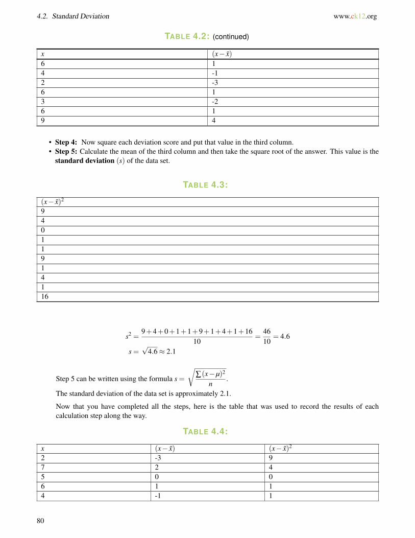
TABLE 4.2: (continued)

x (x− x̄)6 14 -12 -36 13 -26 19 4

• Step 4: Now square each deviation score and put that value in the third column.• Step 5: Calculate the mean of the third column and then take the square root of the answer. This value is the

standard deviation (s) of the data set.

TABLE 4.3:

(x− x̄)2

94011914116

s2 =9+4+0+1+1+9+1+4+1+16

10=

4610

= 4.6

s =√

4.6≈ 2.1

Step 5 can be written using the formula s =

√∑(x−µ)2

n.

The standard deviation of the data set is approximately 2.1.

Now that you have completed all the steps, here is the table that was used to record the results of eachcalculation step along the way.

TABLE 4.4:

x (x− x̄) (x− x̄)2

2 -3 97 2 45 0 06 1 14 -1 1

80

www.ck12.org Chapter 4. Normal Distributions

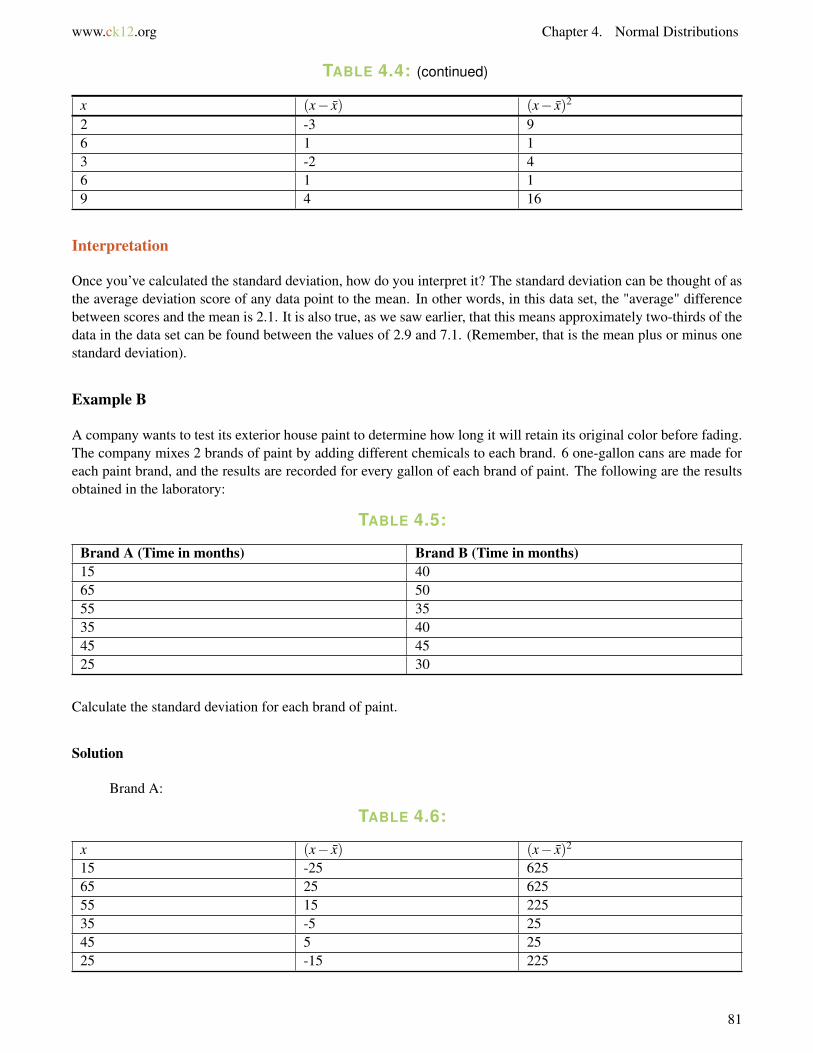
TABLE 4.4: (continued)

x (x− x̄) (x− x̄)2

2 -3 96 1 13 -2 46 1 19 4 16

Interpretation

Once you’ve calculated the standard deviation, how do you interpret it? The standard deviation can be thought of asthe average deviation score of any data point to the mean. In other words, in this data set, the "average" differencebetween scores and the mean is 2.1. It is also true, as we saw earlier, that this means approximately two-thirds of thedata in the data set can be found between the values of 2.9 and 7.1. (Remember, that is the mean plus or minus onestandard deviation).

Example B

A company wants to test its exterior house paint to determine how long it will retain its original color before fading.The company mixes 2 brands of paint by adding different chemicals to each brand. 6 one-gallon cans are made foreach paint brand, and the results are recorded for every gallon of each brand of paint. The following are the resultsobtained in the laboratory:

TABLE 4.5:

Brand A (Time in months) Brand B (Time in months)15 4065 5055 3535 4045 4525 30

Calculate the standard deviation for each brand of paint.

Solution

Brand A:

TABLE 4.6:

x (x− x̄) (x− x̄)2

15 -25 62565 25 62555 15 22535 -5 2545 5 2525 -15 225

81

4.2. Standard Deviation www.ck12.org

x̄ =15+65+55+35+45+25

6=

2406

= 40

s =

√∑(x−µ)2

n

s =

√625+625+225+25+25+225

6

s =

√1750

6≈√

291.66≈ 17.1

The standard deviation for Brand A is approximately 17.1.

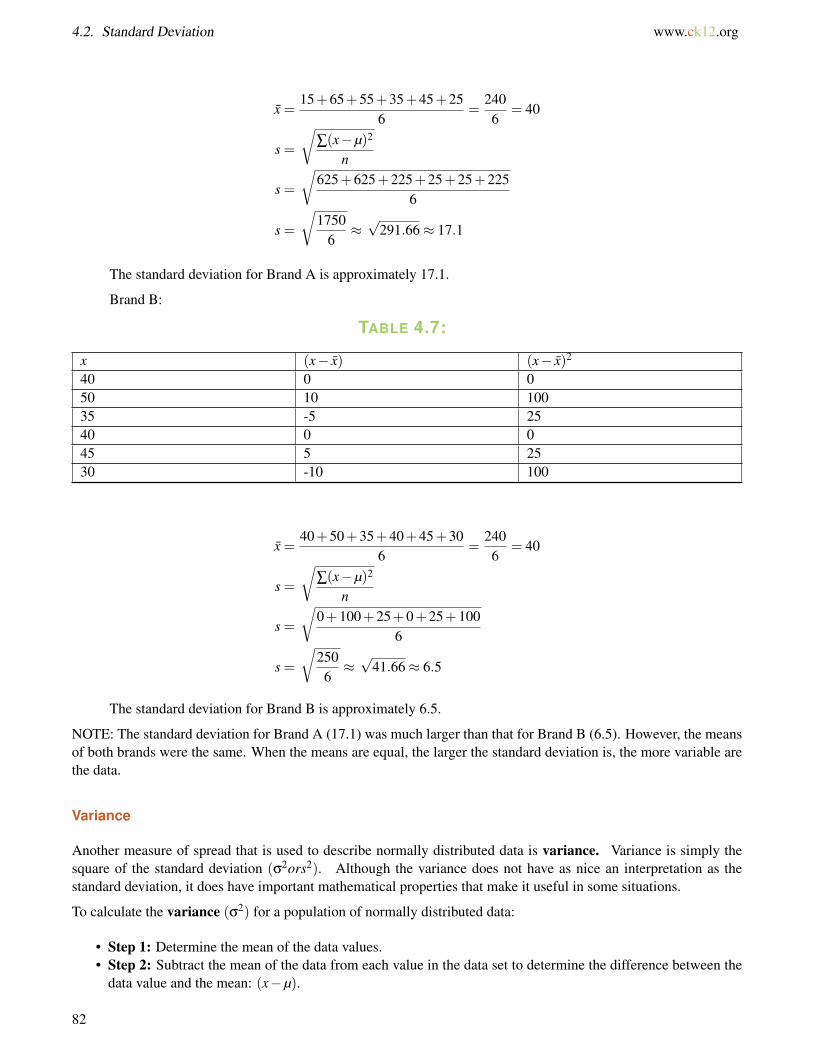
Brand B:

TABLE 4.7:

x (x− x̄) (x− x̄)2

40 0 050 10 10035 -5 2540 0 045 5 2530 -10 100

x̄ =40+50+35+40+45+30

6=

2406

= 40

s =

√∑(x−µ)2

n

s =

√0+100+25+0+25+100

6

s =

√2506≈√

41.66≈ 6.5

The standard deviation for Brand B is approximately 6.5.

NOTE: The standard deviation for Brand A (17.1) was much larger than that for Brand B (6.5). However, the meansof both brands were the same. When the means are equal, the larger the standard deviation is, the more variable arethe data.

Variance

Another measure of spread that is used to describe normally distributed data is variance. Variance is simply thesquare of the standard deviation (σ2ors2). Although the variance does not have as nice an interpretation as thestandard deviation, it does have important mathematical properties that make it useful in some situations.

To calculate the variance (σ2) for a population of normally distributed data:

• Step 1: Determine the mean of the data values.• Step 2: Subtract the mean of the data from each value in the data set to determine the difference between the

data value and the mean: (x−µ).

82

www.ck12.org Chapter 4. Normal Distributions

• Step 3: Square each of these differences and determine the total of these positive, squared results.• Step 4: Divide this sum by the number of values in the data set.

These steps for calculating the variance of a data set for a population can be summarized in the following formula:

σ2 =

∑(x−µ)2

n

where:

x is a data value.

µ is the population mean.

n is number of data values (population size).

These steps for calculating the variance of a data set for a sample can be summarized in the following formula:

s2 =∑(x− x)2

n−1

where:

x is a data value.

x is the sample mean.

n is number of data values (sample size).

The only difference in the formulas is the number by which the sum is divided. For a population, it is divided by n,and for a sample, it is divided by n−1.

Example C

Calculate the variance of the 2 brands of paint in Example B. These are both small populations.

TABLE 4.8:

Brand A (Time in months) Brand B (Time in months)15 4065 5055 3535 4045 4525 30

Solution

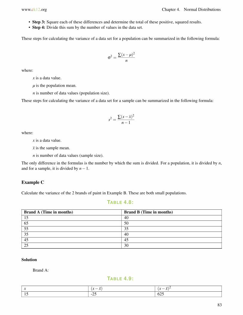
Brand A:

TABLE 4.9:

x (x− x̄) (x− x̄)2

15 -25 625

83

4.2. Standard Deviation www.ck12.org

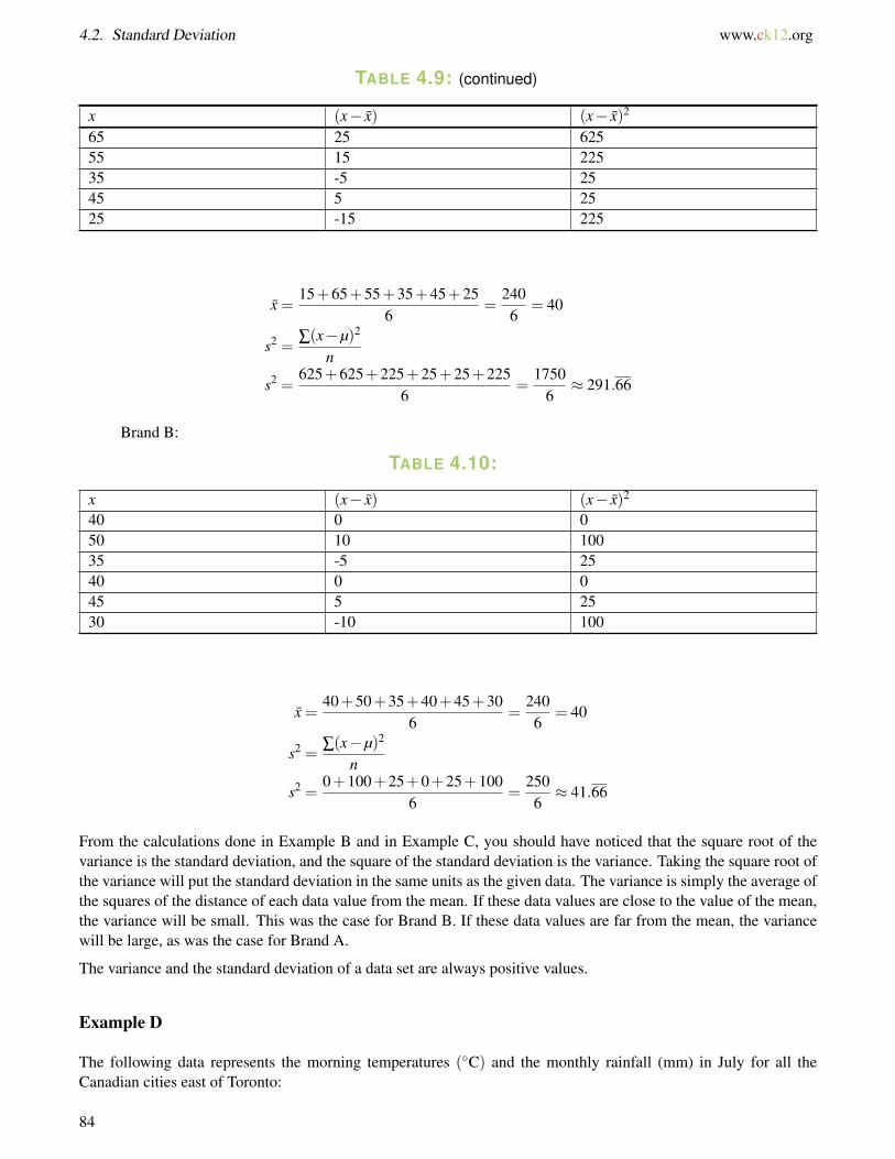
TABLE 4.9: (continued)

x (x− x̄) (x− x̄)2

65 25 62555 15 22535 -5 2545 5 2525 -15 225

x̄ =15+65+55+35+45+25

6=

2406

= 40

s2 =∑(x−µ)2

n

s2 =625+625+225+25+25+225

6=

17506≈ 291.66

Brand B:

TABLE 4.10:

x (x− x̄) (x− x̄)2

40 0 050 10 10035 -5 2540 0 045 5 2530 -10 100

x̄ =40+50+35+40+45+30

6=

2406

= 40

s2 =∑(x−µ)2

n

s2 =0+100+25+0+25+100

6=

2506≈ 41.66

From the calculations done in Example B and in Example C, you should have noticed that the square root of thevariance is the standard deviation, and the square of the standard deviation is the variance. Taking the square root ofthe variance will put the standard deviation in the same units as the given data. The variance is simply the average ofthe squares of the distance of each data value from the mean. If these data values are close to the value of the mean,the variance will be small. This was the case for Brand B. If these data values are far from the mean, the variancewill be large, as was the case for Brand A.

The variance and the standard deviation of a data set are always positive values.

Example D

The following data represents the morning temperatures (◦C) and the monthly rainfall (mm) in July for all theCanadian cities east of Toronto:

84

www.ck12.org Chapter 4. Normal Distributions

Temperature (◦C)

11.7 13.7 10.5 14.2 13.9 14.2 10.4 16.1 16.4

4.8 15.2 13.0 14.4 12.7 8.6 12.9 11.5 14.6

Precipitation (mm)

18.6 37.1 70.9 102 59.9 58.0 73.0 77.6 89.1

86.6 40.3 119.5 36.2 85.5 59.2 97.8 122.2 82.6

Which data set is more variable? Calculate the standard deviation for each data set

Solution

TABLE 4.11: Temperature

x (x− x̄) (x− x̄2

11.7 -1 113.7 1 110.5 -2.2 4.8414.2 1.5 2.2513.9 1.2 1.4414.2 1.5 2.2510.4 -2.3 5.2916.1 3.4 11.5616.4 3.7 13.694.8 -7.9 62.4115.2 2.5 6.2513.0 0.3 0.0914.4 1.7 2.8912.7 0 08.6 -4.1 16.8112.9 0.2 0.0411.5 -1.2 1.4414.6 1.9 3.61

x̄ =∑xn

=228.6

18≈ 12.7

s2 =∑(x−µ)2

ns =

√∑(x−µ)2

n

s2 =136.86

18≈ 7.6 s =

√136.86

18≈ 2.8

The variance of the data set is approximately 7.6 ◦C, and the standard deviation of the data set is approximately2.8 ◦C.

85

4.2. Standard Deviation www.ck12.org

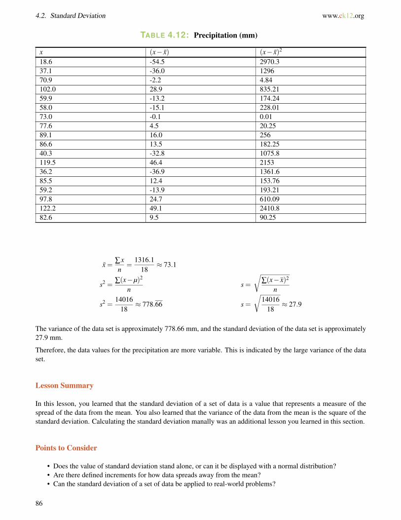
TABLE 4.12: Precipitation (mm)

x (x− x̄) (x− x̄)2

18.6 -54.5 2970.337.1 -36.0 129670.9 -2.2 4.84102.0 28.9 835.2159.9 -13.2 174.2458.0 -15.1 228.0173.0 -0.1 0.0177.6 4.5 20.2589.1 16.0 25686.6 13.5 182.2540.3 -32.8 1075.8119.5 46.4 215336.2 -36.9 1361.685.5 12.4 153.7659.2 -13.9 193.2197.8 24.7 610.09122.2 49.1 2410.882.6 9.5 90.25

x̄ =∑xn

=1316.1

18≈ 73.1

s2 =∑(x−µ)2

ns =

√∑(x− x)2

n

s2 =14016

18≈ 778.66 s =

√14016

18≈ 27.9

The variance of the data set is approximately 778.66 mm, and the standard deviation of the data set is approximately27.9 mm.

Therefore, the data values for the precipitation are more variable. This is indicated by the large variance of the dataset.

Lesson Summary

In this lesson, you learned that the standard deviation of a set of data is a value that represents a measure of thespread of the data from the mean. You also learned that the variance of the data from the mean is the square of thestandard deviation. Calculating the standard deviation manally was an additional lesson you learned in this section.

Points to Consider

• Does the value of standard deviation stand alone, or can it be displayed with a normal distribution?• Are there defined increments for how data spreads away from the mean?• Can the standard deviation of a set of data be applied to real-world problems?

86

www.ck12.org Chapter 4. Normal Distributions

Review Questions

1. Without using technology, calculate the variance and the standard deviation of each of the following sets ofnumbers.

1. a. 2,4,6,8,10,12,14,16,18,20b. 18,23,23,25,29,33,35,35c. 123,134,134,139,145,147,151,155,157d. 58,58,65,66,69,70,70,76,79,80,83

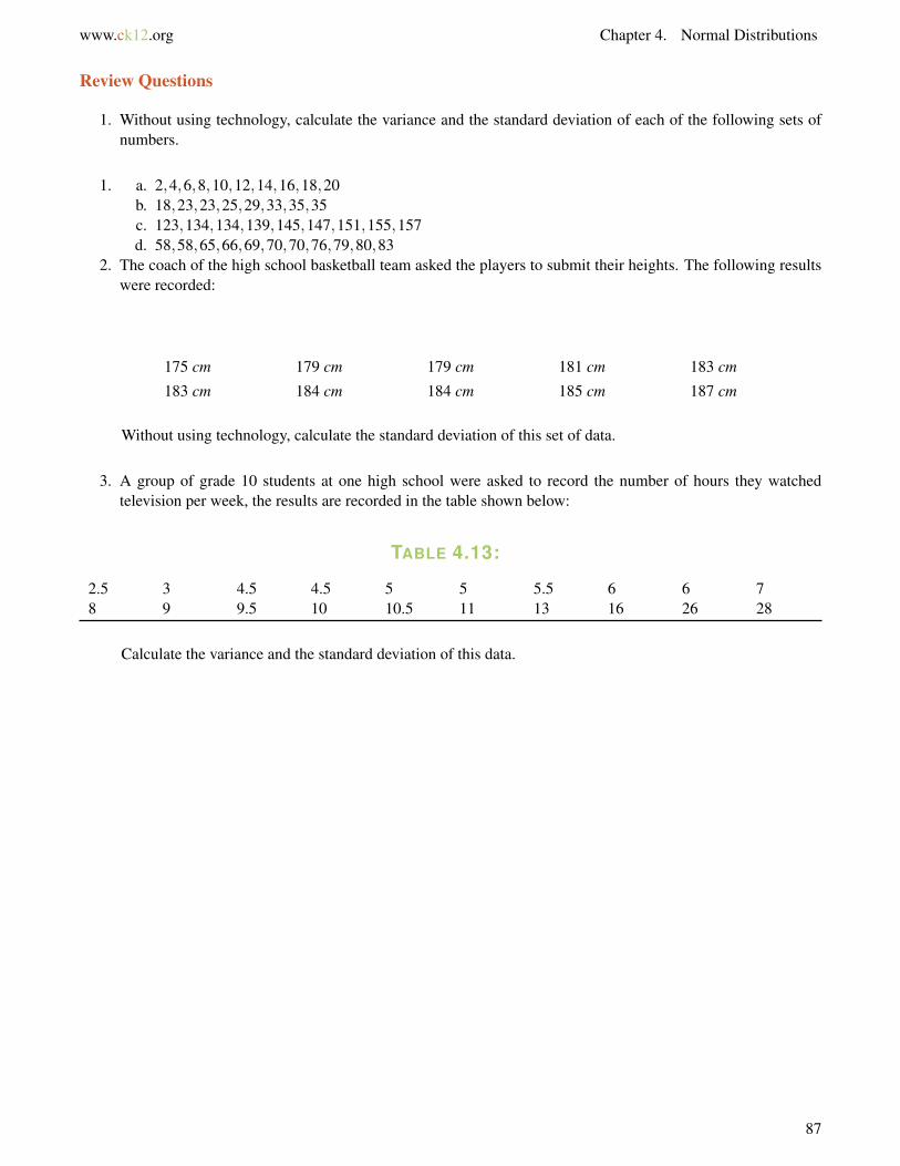
2. The coach of the high school basketball team asked the players to submit their heights. The following resultswere recorded:

175 cm 179 cm 179 cm 181 cm 183 cm

183 cm 184 cm 184 cm 185 cm 187 cm

Without using technology, calculate the standard deviation of this set of data.

3. A group of grade 10 students at one high school were asked to record the number of hours they watchedtelevision per week, the results are recorded in the table shown below:

TABLE 4.13:

2.5 3 4.5 4.5 5 5 5.5 6 6 78 9 9.5 10 10.5 11 13 16 26 28

Calculate the variance and the standard deviation of this data.

87

4.3. The Empirical Rule www.ck12.org

4.3 The Empirical Rule

Learning Objectives

• Apply the Empirical Rule to questions about normal distributions.• Use the percentages associated with normal distribution to solve problems.

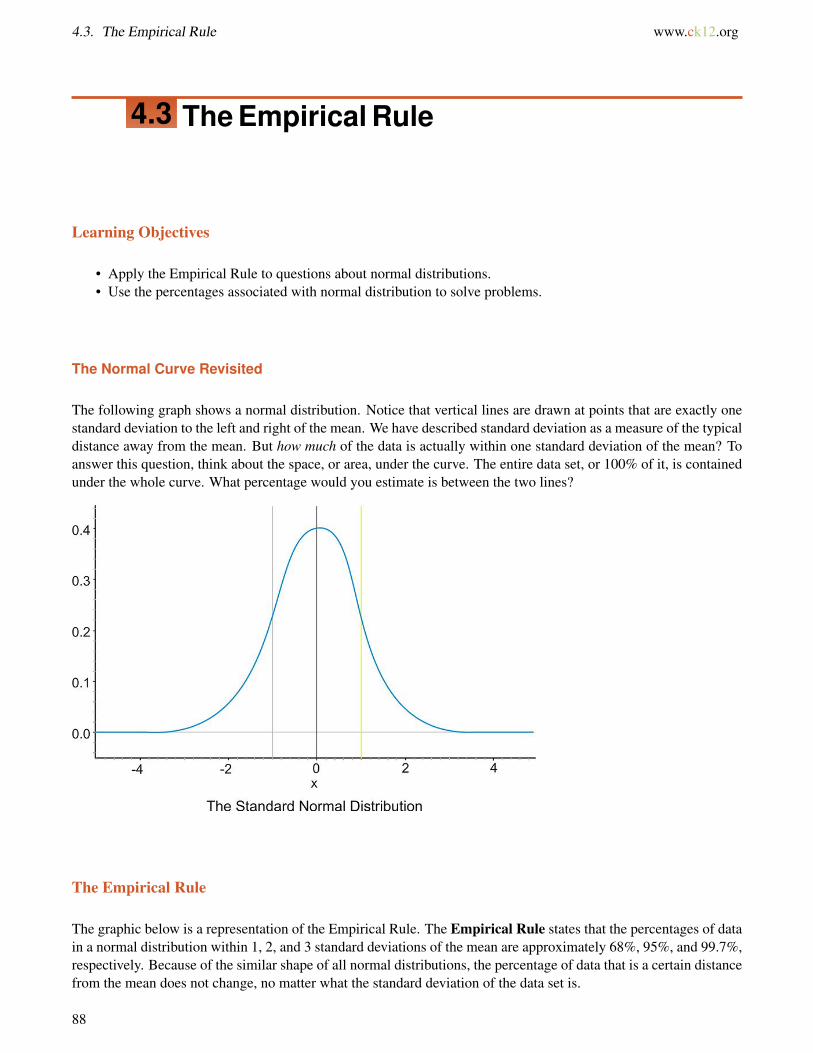
The Normal Curve Revisited

The following graph shows a normal distribution. Notice that vertical lines are drawn at points that are exactly onestandard deviation to the left and right of the mean. We have described standard deviation as a measure of the typicaldistance away from the mean. But how much of the data is actually within one standard deviation of the mean? Toanswer this question, think about the space, or area, under the curve. The entire data set, or 100% of it, is containedunder the whole curve. What percentage would you estimate is between the two lines?

The Empirical Rule

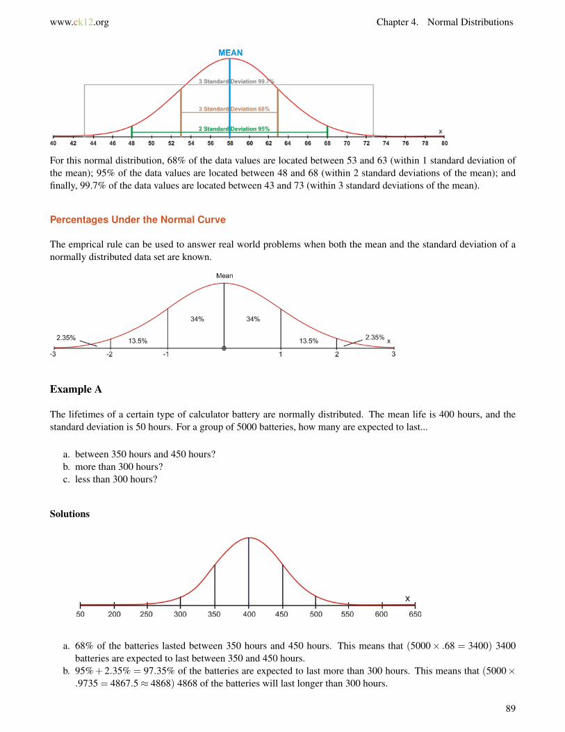
The graphic below is a representation of the Empirical Rule. The Empirical Rule states that the percentages of datain a normal distribution within 1, 2, and 3 standard deviations of the mean are approximately 68%, 95%, and 99.7%,respectively. Because of the similar shape of all normal distributions, the percentage of data that is a certain distancefrom the mean does not change, no matter what the standard deviation of the data set is.

88

www.ck12.org Chapter 4. Normal Distributions

For this normal distribution, 68% of the data values are located between 53 and 63 (within 1 standard deviation ofthe mean); 95% of the data values are located between 48 and 68 (within 2 standard deviations of the mean); andfinally, 99.7% of the data values are located between 43 and 73 (within 3 standard deviations of the mean).

Percentages Under the Normal Curve

The emprical rule can be used to answer real world problems when both the mean and the standard deviation of anormally distributed data set are known.

Example A

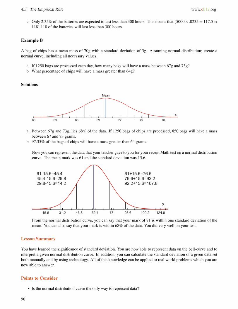
The lifetimes of a certain type of calculator battery are normally distributed. The mean life is 400 hours, and thestandard deviation is 50 hours. For a group of 5000 batteries, how many are expected to last...

a. between 350 hours and 450 hours?b. more than 300 hours?c. less than 300 hours?

Solutions

a. 68% of the batteries lasted between 350 hours and 450 hours. This means that (5000× .68 = 3400) 3400batteries are expected to last between 350 and 450 hours.

b. 95%+ 2.35% = 97.35% of the batteries are expected to last more than 300 hours. This means that (5000×.9735 = 4867.5≈ 4868) 4868 of the batteries will last longer than 300 hours.

89

4.3. The Empirical Rule www.ck12.org

c. Only 2.35% of the batteries are expected to last less than 300 hours. This means that (5000× .0235 = 117.5≈118) 118 of the batteries will last less than 300 hours.

Example B

A bag of chips has a mean mass of 70g with a standard deviation of 3g. Assuming normal distribution; create anormal curve, including all necessary values.

a. If 1250 bags are processed each day, how many bags will have a mass between 67g and 73g?b. What percentage of chips will have a mass greater than 64g?

Solutions

a. Between 67g and 73g, lies 68% of the data. If 1250 bags of chips are processed, 850 bags will have a massbetween 67 and 73 grams.

b. 97.35% of the bags of chips will have a mass greater than 64 grams.

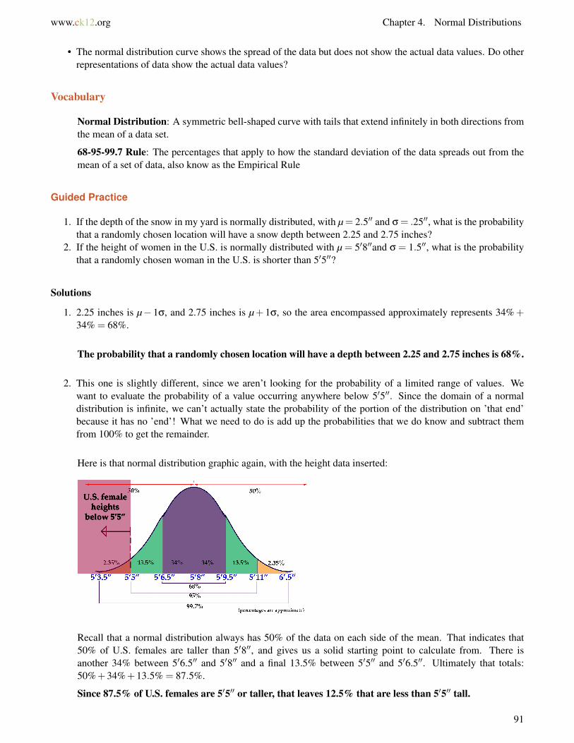
Now you can represent the data that your teacher gave to you for your recent Math test on a normal distributioncurve. The mean mark was 61 and the standard deviation was 15.6.

From the normal distribution curve, you can say that your mark of 71 is within one standard deviation of themean. You can also say that your mark is within 68% of the data. You did very well on your test.

Lesson Summary

You have learned the significance of standard deviation. You are now able to represent data on the bell-curve and tointerpret a given normal distribution curve. In addition, you can calculate the standard deviation of a given data setboth manually and by using technology. All of this knowledge can be applied to real world problems which you arenow able to answer.

Points to Consider

• Is the normal distribution curve the only way to represent data?

90

www.ck12.org Chapter 4. Normal Distributions

• The normal distribution curve shows the spread of the data but does not show the actual data values. Do otherrepresentations of data show the actual data values?

Vocabulary

Normal Distribution: A symmetric bell-shaped curve with tails that extend infinitely in both directions fromthe mean of a data set.

68-95-99.7 Rule: The percentages that apply to how the standard deviation of the data spreads out from themean of a set of data, also know as the Empirical Rule

Guided Practice

1. If the depth of the snow in my yard is normally distributed, with µ = 2.5′′ and σ = .25′′, what is the probabilitythat a randomly chosen location will have a snow depth between 2.25 and 2.75 inches?

2. If the height of women in the U.S. is normally distributed with µ = 5′8′′and σ = 1.5′′, what is the probabilitythat a randomly chosen woman in the U.S. is shorter than 5′5′′?

Solutions

1. 2.25 inches is µ− 1σ, and 2.75 inches is µ+ 1σ, so the area encompassed approximately represents 34%+34% = 68%.

The probability that a randomly chosen location will have a depth between 2.25 and 2.75 inches is 68%.

2. This one is slightly different, since we aren’t looking for the probability of a limited range of values. Wewant to evaluate the probability of a value occurring anywhere below 5′5′′. Since the domain of a normaldistribution is infinite, we can’t actually state the probability of the portion of the distribution on ’that end’because it has no ’end’! What we need to do is add up the probabilities that we do know and subtract themfrom 100% to get the remainder.

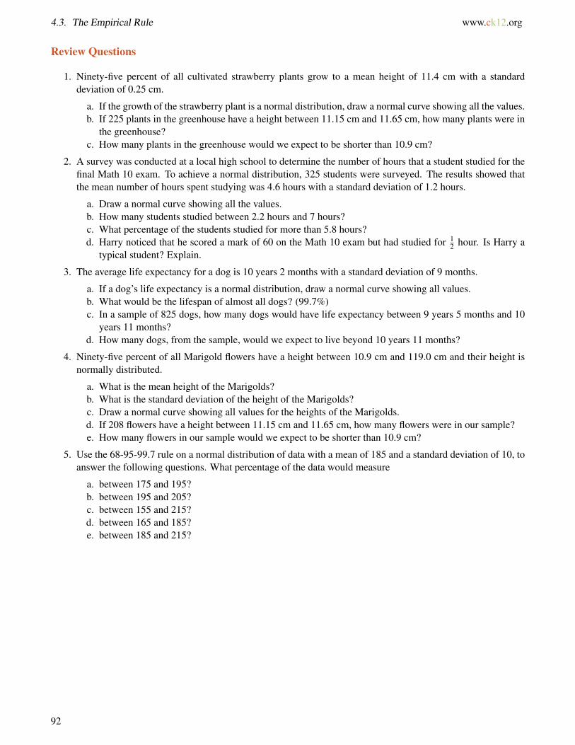
Here is that normal distribution graphic again, with the height data inserted:

Recall that a normal distribution always has 50% of the data on each side of the mean. That indicates that50% of U.S. females are taller than 5′8′′, and gives us a solid starting point to calculate from. There isanother 34% between 5′6.5′′ and 5′8′′ and a final 13.5% between 5′5′′ and 5′6.5′′. Ultimately that totals:50%+34%+13.5% = 87.5%.

Since 87.5% of U.S. females are 5′5′′ or taller, that leaves 12.5% that are less than 5′5′′ tall.

91

4.3. The Empirical Rule www.ck12.org

Review Questions

1. Ninety-five percent of all cultivated strawberry plants grow to a mean height of 11.4 cm with a standarddeviation of 0.25 cm.

a. If the growth of the strawberry plant is a normal distribution, draw a normal curve showing all the values.b. If 225 plants in the greenhouse have a height between 11.15 cm and 11.65 cm, how many plants were in

the greenhouse?c. How many plants in the greenhouse would we expect to be shorter than 10.9 cm?

2. A survey was conducted at a local high school to determine the number of hours that a student studied for thefinal Math 10 exam. To achieve a normal distribution, 325 students were surveyed. The results showed thatthe mean number of hours spent studying was 4.6 hours with a standard deviation of 1.2 hours.

a. Draw a normal curve showing all the values.b. How many students studied between 2.2 hours and 7 hours?c. What percentage of the students studied for more than 5.8 hours?d. Harry noticed that he scored a mark of 60 on the Math 10 exam but had studied for 1

2 hour. Is Harry atypical student? Explain.

3. The average life expectancy for a dog is 10 years 2 months with a standard deviation of 9 months.

a. If a dog’s life expectancy is a normal distribution, draw a normal curve showing all values.b. What would be the lifespan of almost all dogs? (99.7%)c. In a sample of 825 dogs, how many dogs would have life expectancy between 9 years 5 months and 10

years 11 months?d. How many dogs, from the sample, would we expect to live beyond 10 years 11 months?

4. Ninety-five percent of all Marigold flowers have a height between 10.9 cm and 119.0 cm and their height isnormally distributed.

a. What is the mean height of the Marigolds?b. What is the standard deviation of the height of the Marigolds?c. Draw a normal curve showing all values for the heights of the Marigolds.d. If 208 flowers have a height between 11.15 cm and 11.65 cm, how many flowers were in our sample?e. How many flowers in our sample would we expect to be shorter than 10.9 cm?

5. Use the 68-95-99.7 rule on a normal distribution of data with a mean of 185 and a standard deviation of 10, toanswer the following questions. What percentage of the data would measure

a. between 175 and 195?b. between 195 and 205?c. between 155 and 215?d. between 165 and 185?e. between 185 and 215?

92

www.ck12.org Chapter 4. Normal Distributions

4.4 Z-Scores

Learning Objective

• Transform a score into a z-score.• Use the z-table to identify the probability of observing a score less than or greater than a particular value.• Use the z-table to identify the area under a normal curve that falls between two z-scores.• Interpret what a z-score says in terms of how likely (or unlikely) that value is to be observed.

z-Scores

A z -score is a measure of the number of standard deviations a particular data point is away from the mean. Forexample, let’s say the mean score on a test for your statistics class was an 82, with a standard deviation of 7 points.If your score was an 89, it is exactly one standard deviation to the right of the mean; therefore, your z-score wouldbe 1. If, on the other hand, you scored a 75, your score would be exactly one standard deviation below the mean,and your z-score would be −1. All values that are below the mean have negative z-scores, while all values that areabove the mean have positive z-scores. A z-score of −2 would represent a value that is exactly 2 standard deviationsbelow the mean, so in this case, the value would be 82−14 = 68.

To calculate a z-score for which the numbers are not so obvious, you take the deviation and divide it by the standarddeviation.

z =Deviation

Standard Deviation

You may recall that deviation is the mean value of the variable subtracted from the observed value, so in symbolicterms, the z-score would be:

z =x−µ

σ

As previously stated, since σ is always positive, z will be positive when x is greater than µ and negative when x isless than µ. A z-score of zero means that the term has the same value as the mean. The value of z represents thenumber of standard deviations the given value of x is above or below the mean.

Example A

What is the z-score for an A on the test described above, which has a mean score of 82? (Assume that an A is a 93.)

The z-score can be calculated as follows:

z =x−µ

σ

z =93−82

7

z =117≈ 1.57

93

4.4. Z-Scores www.ck12.org

If we know that the test scores from the last example are distributed normally, then a z-score can tell us somethingabout how our test score relates to the rest of the class. From the Empirical Rule, we know that about 68% of thestudents would have scored between a z-score of −1 and 1, or between a 75 and an 89, on the test. If 68% of thedata is between these two values, then that leaves the remaining 32% in the tail areas. Because of symmetry, half ofthis, or 16%, would be in each individual tail.

Example B

On a nationwide math test, the mean was 65 and the standard deviation was 10. If Robert scored 81, what was hisz-score?

z =x−µ

σ

z =81−65

10

z =1610

z = 1.6

Example C

On a college entrance exam, the mean was 70, and the standard deviation was 8. If Helen’s z-score was −1.5, whatwas her exam score?

z =x−µ

σ

∴ z ·σ = x−µ

x = µ+ z ·σx = 70+(−1.5)(8)

x = 58

z-Scores and Probability

Knowing the z-score of a given value is great, but what can you do with it? How does a z-score relate to probability?For example, how likely (or unlikely) is an occurrence of a z-score of 2.47 or greater?

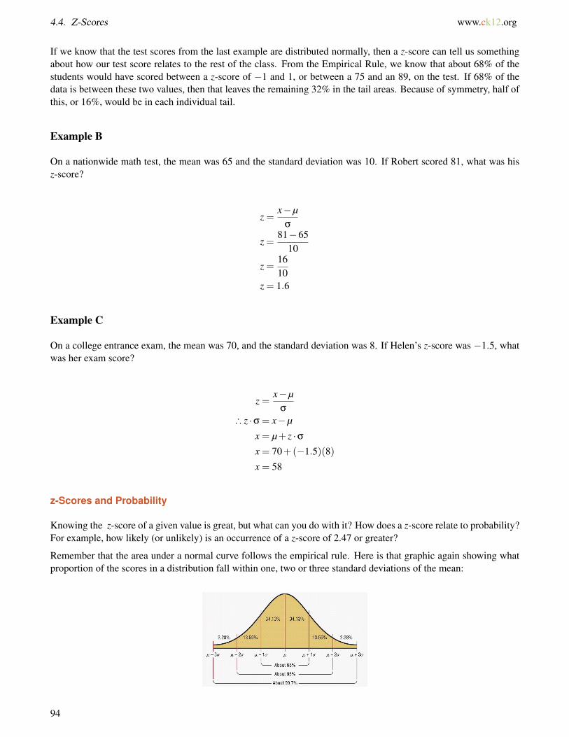
Remember that the area under a normal curve follows the empirical rule. Here is that graphic again showing whatproportion of the scores in a distribution fall within one, two or three standard deviations of the mean:

94

www.ck12.org Chapter 4. Normal Distributions

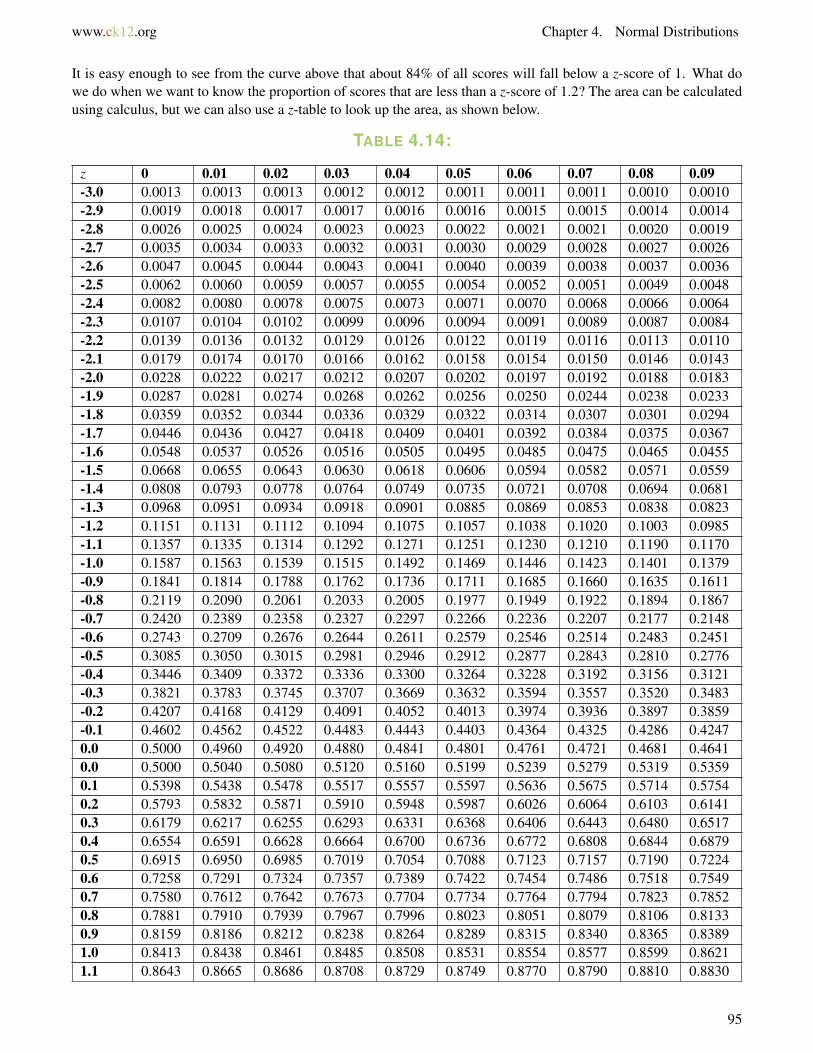
It is easy enough to see from the curve above that about 84% of all scores will fall below a z-score of 1. What dowe do when we want to know the proportion of scores that are less than a z-score of 1.2? The area can be calculatedusing calculus, but we can also use a z-table to look up the area, as shown below.

TABLE 4.14:

z 0 0.01 0.02 0.03 0.04 0.05 0.06 0.07 0.08 0.09-3.0 0.0013 0.0013 0.0013 0.0012 0.0012 0.0011 0.0011 0.0011 0.0010 0.0010-2.9 0.0019 0.0018 0.0017 0.0017 0.0016 0.0016 0.0015 0.0015 0.0014 0.0014-2.8 0.0026 0.0025 0.0024 0.0023 0.0023 0.0022 0.0021 0.0021 0.0020 0.0019-2.7 0.0035 0.0034 0.0033 0.0032 0.0031 0.0030 0.0029 0.0028 0.0027 0.0026-2.6 0.0047 0.0045 0.0044 0.0043 0.0041 0.0040 0.0039 0.0038 0.0037 0.0036-2.5 0.0062 0.0060 0.0059 0.0057 0.0055 0.0054 0.0052 0.0051 0.0049 0.0048-2.4 0.0082 0.0080 0.0078 0.0075 0.0073 0.0071 0.0070 0.0068 0.0066 0.0064-2.3 0.0107 0.0104 0.0102 0.0099 0.0096 0.0094 0.0091 0.0089 0.0087 0.0084-2.2 0.0139 0.0136 0.0132 0.0129 0.0126 0.0122 0.0119 0.0116 0.0113 0.0110-2.1 0.0179 0.0174 0.0170 0.0166 0.0162 0.0158 0.0154 0.0150 0.0146 0.0143-2.0 0.0228 0.0222 0.0217 0.0212 0.0207 0.0202 0.0197 0.0192 0.0188 0.0183-1.9 0.0287 0.0281 0.0274 0.0268 0.0262 0.0256 0.0250 0.0244 0.0238 0.0233-1.8 0.0359 0.0352 0.0344 0.0336 0.0329 0.0322 0.0314 0.0307 0.0301 0.0294-1.7 0.0446 0.0436 0.0427 0.0418 0.0409 0.0401 0.0392 0.0384 0.0375 0.0367-1.6 0.0548 0.0537 0.0526 0.0516 0.0505 0.0495 0.0485 0.0475 0.0465 0.0455-1.5 0.0668 0.0655 0.0643 0.0630 0.0618 0.0606 0.0594 0.0582 0.0571 0.0559-1.4 0.0808 0.0793 0.0778 0.0764 0.0749 0.0735 0.0721 0.0708 0.0694 0.0681-1.3 0.0968 0.0951 0.0934 0.0918 0.0901 0.0885 0.0869 0.0853 0.0838 0.0823-1.2 0.1151 0.1131 0.1112 0.1094 0.1075 0.1057 0.1038 0.1020 0.1003 0.0985-1.1 0.1357 0.1335 0.1314 0.1292 0.1271 0.1251 0.1230 0.1210 0.1190 0.1170-1.0 0.1587 0.1563 0.1539 0.1515 0.1492 0.1469 0.1446 0.1423 0.1401 0.1379-0.9 0.1841 0.1814 0.1788 0.1762 0.1736 0.1711 0.1685 0.1660 0.1635 0.1611-0.8 0.2119 0.2090 0.2061 0.2033 0.2005 0.1977 0.1949 0.1922 0.1894 0.1867-0.7 0.2420 0.2389 0.2358 0.2327 0.2297 0.2266 0.2236 0.2207 0.2177 0.2148-0.6 0.2743 0.2709 0.2676 0.2644 0.2611 0.2579 0.2546 0.2514 0.2483 0.2451-0.5 0.3085 0.3050 0.3015 0.2981 0.2946 0.2912 0.2877 0.2843 0.2810 0.2776-0.4 0.3446 0.3409 0.3372 0.3336 0.3300 0.3264 0.3228 0.3192 0.3156 0.3121-0.3 0.3821 0.3783 0.3745 0.3707 0.3669 0.3632 0.3594 0.3557 0.3520 0.3483-0.2 0.4207 0.4168 0.4129 0.4091 0.4052 0.4013 0.3974 0.3936 0.3897 0.3859-0.1 0.4602 0.4562 0.4522 0.4483 0.4443 0.4403 0.4364 0.4325 0.4286 0.42470.0 0.5000 0.4960 0.4920 0.4880 0.4841 0.4801 0.4761 0.4721 0.4681 0.46410.0 0.5000 0.5040 0.5080 0.5120 0.5160 0.5199 0.5239 0.5279 0.5319 0.53590.1 0.5398 0.5438 0.5478 0.5517 0.5557 0.5597 0.5636 0.5675 0.5714 0.57540.2 0.5793 0.5832 0.5871 0.5910 0.5948 0.5987 0.6026 0.6064 0.6103 0.61410.3 0.6179 0.6217 0.6255 0.6293 0.6331 0.6368 0.6406 0.6443 0.6480 0.65170.4 0.6554 0.6591 0.6628 0.6664 0.6700 0.6736 0.6772 0.6808 0.6844 0.68790.5 0.6915 0.6950 0.6985 0.7019 0.7054 0.7088 0.7123 0.7157 0.7190 0.72240.6 0.7258 0.7291 0.7324 0.7357 0.7389 0.7422 0.7454 0.7486 0.7518 0.75490.7 0.7580 0.7612 0.7642 0.7673 0.7704 0.7734 0.7764 0.7794 0.7823 0.78520.8 0.7881 0.7910 0.7939 0.7967 0.7996 0.8023 0.8051 0.8079 0.8106 0.81330.9 0.8159 0.8186 0.8212 0.8238 0.8264 0.8289 0.8315 0.8340 0.8365 0.83891.0 0.8413 0.8438 0.8461 0.8485 0.8508 0.8531 0.8554 0.8577 0.8599 0.86211.1 0.8643 0.8665 0.8686 0.8708 0.8729 0.8749 0.8770 0.8790 0.8810 0.8830

95

4.4. Z-Scores www.ck12.org

TABLE 4.14: (continued)

1.2 0.8849 0.8869 0.8888 0.8907 0.8925 0.8944 0.8962 0.8980 0.8997 0.90151.3 0.9032 0.9049 0.9066 0.9082 0.9099 0.9115 0.9131 0.9147 0.9162 0.91771.4 0.9192 0.9207 0.9222 0.9236 0.9251 0.9265 0.9279 0.9292 0.9306 0.93191.5 0.9332 0.9345 0.9357 0.9370 0.9382 0.9394 0.9406 0.9418 0.9430 0.94411.6 0.9452 0.9463 0.9474 0.9485 0.9495 0.9505 0.9515 0.9525 0.9535 0.95451.7 0.9554 0.9564 0.9573 0.9582 0.9591 0.9599 0.9608 0.9616 0.9625 0.96331.8 0.9641 0.9649 0.9656 0.9664 0.9671 0.9678 0.9686 0.9693 0.9700 0.97061.9 0.9713 0.9719 0.9726 0.9732 0.9738 0.9744 0.9750 0.9756 0.9762 0.97672.0 0.9773 0.9778 0.9783 0.9788 0.9793 0.9798 0.9803 0.9808 0.9812 0.98172.1 0.9821 0.9826 0.9830 0.9834 0.9838 0.9842 0.9846 0.9850 0.9854 0.98572.2 0.9861 0.9865 0.9868 0.9871 0.9875 0.9878 0.9881 0.9884 0.9887 0.98902.3 0.9893 0.9896 0.9898 0.9901 0.9904 0.9906 0.9909 0.9911 0.9913 0.99162.4 0.9918 0.9920 0.9922 0.9925 0.9927 0.9929 0.9931 0.9932 0.9934 0.99362.5 0.9938 0.9940 0.9941 0.9943 0.9945 0.9946 0.9948 0.9949 0.9951 0.99522.6 0.9953 0.9955 0.9956 0.9957 0.9959 0.9960 0.9961 0.9962 0.9963 0.99642.7 0.9965 0.9966 0.9967 0.9968 0.9969 0.9970 0.9971 0.9972 0.9973 0.99742.8 0.9974 0.9975 0.9976 0.9977 0.9977 0.9978 0.9979 0.9980 0.9980 0.99812.9 0.9981 0.9982 0.9983 0.9983 0.9984 0.9984 0.9985 0.9985 0.9986 0.99863.0 0.9987 0.9987 0.9987 0.9988 0.9988 0.9989 0.9989 0.9989 0.9990 0.9990

Finding the Probability Associated with a z-Score

The z-score table above provides the area under the standard normal distribution that falls to the left of each particularz value. That is the value shaded in the diagram below. The area can be interpreted as the probability that a score inthe distribution is less than the score that corresponds to z.

FIGURE 4.1

For example, a z-score of zero (remember that is the z-score that corresponds to the mean), has a probability of 0.5because half of the scores in the normal distribution are lower than the mean. Although the table only provides thearea to the left of each z value, remember that the area under the entire standard normal distribution is equal to one.So to find the probability of getting a value greater than z, look up the probability for z in the table and subtract itfrom one.

96

www.ck12.org Chapter 4. Normal Distributions

Example A

What is the probability that a value with a z-score less than 2.47 will occur in a normal distribution?

Solution

Scroll up to the table above and find “2.4” on the left or right side. Now move across the table to “0.07” on the topor bottom, and record the value in the cell: 0.9932. That tells us that 99.32% of values in the set are at or below az -score of 2.47.

Example B

What is the probability that a value with a z-score greater than 1.53 will occur in a normal distribution?

Solution

Scroll up to the table of z-score probabilities again and find the intersection between 1.5 on the left or right and 3 onthe top or bottom, record the value in the cell: 0.937 .

That decimal lets us know that 93.7% of values in the set are below the z-score of 1.53. To find the percentage thatis above that value, we subtract 0.937 from 1.0 (or 93.7% from 100%), to get 0.063 or 6.3%.

Example C

What is the probability of a random selection being less than 3.65, given a normal distribution with µ = 5 andσ = 2.2?

Solution

This question requires us to first find the z-score for the value 3.65, then calculate the percentage of values belowthat z-score from a reference.

1. Find the z -score for 3.65, using the z-score formula: (x−µ)σ

z =3.65−5

2.2=−1.35

2.2≈−0.61

2. Now we can scroll up to our z-score reference above and find the intersection of -0.6 and 0.01, which shouldbe .2709

There is approximately a 27.09% probability that a value less than 3.65 would occur from a random selection of anormal distribution with mean 5 and standard deviation 2.2.

Finding the Probability Between Two z-Scores

How would you calculate the proportion of scores that fall between z-scores of -0.08 and +1.92? We can do this bylooking up each probability separately and subtracting.

97

4.4. Z-Scores www.ck12.org

Example A

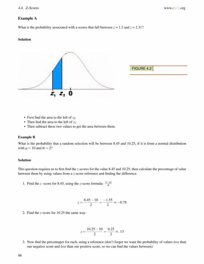
What is the probability associated with a scores that fall between z = 1.2 and z = 2.31?

Solution

FIGURE 4.2

• First find the area to the left of z2.• Then find the area to the left of z1.• Then subtract these two values to get the area between them.

Example B

What is the probability that a random selection will be between 8.45 and 10.25, if it is from a normal distributionwith µ = 10 and σ = 2?

Solution

This question requires us to first find the z-scores for the value 8.45 and 10.25, then calculate the percentage of valuebetween them by using values from a z-score reference and finding the difference.

1. Find the z -score for 8.45, using the z-score formula: (x−µ)σ

z =8.45−10

2=−1.55

2≈−0.78

2. Find the z-score for 10.25 the same way:

z =10.25−10

2=

0.252≈ .13

3. Now find the percentages for each, using a reference (don’t forget we want the probability of values less thanour negative score and less than our positive score, so we can find the values between):

98

www.ck12.org Chapter 4. Normal Distributions

P(Z <−0.78) = .2177 or 21.77%

P(Z < .13) = .5517 or 55.17%

4. At this point, let’s sketch the graph to get an idea what we are looking for:

5. Finally, subtract the values to find the difference:

p = .5517− .2177 = .3340 or about 33.4%

There is approximately a 33.4% probability that a value between 8.45 and 10.25 would result from a random selectionof a normal distribution with mean 10 and standard deviation 2.

Vocabulary

A z -score is a measure of how many standard deviations there are between a data value and the mean.

A z -score probability table is a table that associates z-scores to area under the normal curve. The table maybe used to associate a Z-score with a percent probability.

Guided Practice with z-Score Calculations

1. What is the z-score of the price of a pair of skis that cost $247, if the mean ski price is $279, with a standarddeviation of $16?

2. What is the z-score of a 5-scoop ice cream cone if the mean number of scoops is 3, with a standard deviationof 1 scoop?

3. What is the z-score of the weight of a cow that tips the scales at 825 lbs, if the mean weight for cows of hertype is 1150 lbs, with a standard deviation of 77 lbs?

4. What is the z-score of a measured value of 0.0034, given µ = 0.0041 and σ = 0.0008?

99

4.4. Z-Scores www.ck12.org

Solutions

1. First find the difference between the measured value and the mean, then divide that difference by the standarddeviation:

z =247−279

16

z =−3216

z =−2

2. This one is easy: The difference between 5 scoops and 3 scoops is +2, and we divide that by the standarddeviation of 1, so the z -score is +2.

3. First find the difference between the measured value and the mean, then divide that difference by the standarddeviation:

z =825 lbs−1150 lbs

771 lbs

z =−325

77z =−4.2207

4. First find the difference between the measured value and the mean, then divide that difference by the standarddeviation:

z =0.0034−0.0041

0.0008

z =−0.00070.0008

z =−0.875

Guided Practice with z-Table

1. What is the probability of occurrence of a value with z-score greater than 1.24?2. What is the probability of z <−.23?3. What is P(Z < 2.13)?

Solutions

1. Since this is a positive z-score, we can use the value for z = 1.24 directly from the table, and just express it asa percentage: 0.8925 or 89.25%

2. This is a negative z-score : 40.9%3. This is a positive z-score, and we need the percentage of values below it, so we can use the percentage

associated with z =+2.13 directly from the table: 0.9834 or 98.34%

100

www.ck12.org Chapter 4. Normal Distributions

Guided Practice with Probability between two z-Scores

1. What is the probability of a z-score between -0.93 and 2.11?2. What is P(1.39 < Z < 2.03)?

Solutions

1. Using the z-score probability table above, we can see that the probability of a value below -0.93 is .1762,and the probability of a value below 2.11 is .9826. Therefore, the probability of a value between them is.9826− .1762 = .8064 or 80.64%

2. Using the z-score probability table, we see that the probability of a value below z = 1.39 is .9177, and avalue below z = 2.03 is .9788. That means that the probability of a value between them is .9788− .9177 =.0611 or 6.11%

More Practice

1. Given a distribution with a mean of 70 and standard deviation of 62, find a value with a z-score of -1.82.2. What does a z-score of 3.4 mean?3. Given a distribution with a mean of 60 and standard deviation of 98, find the z-score of 120.76.4. Given a distribution with a mean of 60 and standard deviation of 21, find a value with a z-score of 2.19.5. Find the z-score of 187.37, given a distribution with a mean of 185 and standard deviation of 1.6. What is the probability of a z-score between +1.99 and +2.02?7. What is the probability of a z-score between -1.99 and +2.02?8. What is the probability of a z-score between -1.20 and -1.97?9. What is the probability of a z-score between +2.33 and-0.97?

10. What is the probability of a z-score greater than +0.09?11. What is the probability of a z-score greater than -0.02?12. What is P(1.42 < Z < 2.01)?13. What is the probability of the random occurrence of a value between 56 and 61 from a normally distributed

population with mean 62 and standard deviation 4.5?14. What is the probability of a value between 301 and 329, assuming a normally distributed set with mean 290

and standard deviation 32?15. What is the probability of getting a value between 1.2 and 2.3 from the random output of a normally distributed

set with µ = 2.6and σ = .9?

101