More About Significance More About Significance TestsTests

Presentation 11

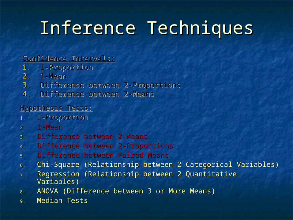
Inference TechniquesInference Techniques

Hypothesis Tests:Hypothesis Tests:1.1. 1-Proportion1-Proportion2.2. 1-Mean1-Mean3.3. Difference between 2-MeansDifference between 2-Means4.4. Difference between 2-ProportionsDifference between 2-Proportions5.5. Difference between Paired Means.Difference between Paired Means.6.6. Chi-Square (Relationship between 2 Categorical Variables)Chi-Square (Relationship between 2 Categorical Variables)7.7. Regression (Relationship between 2 Quantitative Variables)Regression (Relationship between 2 Quantitative Variables)8.8. ANOVA (Difference between 3 or More Means)ANOVA (Difference between 3 or More Means)9.9. Median TestsMedian Tests

Confidence Intervals:Confidence Intervals:1.1. 1-Proportion1-Proportion2.2. 1-Mean1-Mean3.3. Difference between 2-ProportionsDifference between 2-Proportions4.4. Difference between 2-MeansDifference between 2-Means

General Steps for Hypothesis General Steps for Hypothesis TestsTests

Step 1: Determine the HStep 1: Determine the H00 and H and Ha.a.

The alternative hypothesis, HThe alternative hypothesis, Haa, is the claim regarding the , is the claim regarding the population parameter that we want to test. There are three population parameter that we want to test. There are three possible Hpossible Haa's - the parameter is not equal to a null value (two-'s - the parameter is not equal to a null value (two-sided), less than a null value (one-sided) or greater than a null sided), less than a null value (one-sided) or greater than a null value (one-sided). The null hypothesis, Hvalue (one-sided). The null hypothesis, H00, claims that nothing is , claims that nothing is happening. Hhappening. H00 can be the opposite of H can be the opposite of Haa or just that the parameter or just that the parameter is equal to the null value.is equal to the null value.

Step 2: Verify necessary data conditions, if met Step 2: Verify necessary data conditions, if met summarize the data into an appropriate test statistic.summarize the data into an appropriate test statistic.

The conditions to be verified are the same conditions we have seen The conditions to be verified are the same conditions we have seen in Chapter 12 for creating C.I's. in Chapter 12 for creating C.I's.

The The test statistictest statistic is a standardized statistic, i.e. is of the form is a standardized statistic, i.e. is of the form

Sample statistic - Null valueSample statistic - Null valueNull s.e (sample statistic)Null s.e (sample statistic)

Under HUnder H00 the test statistic follows either a normal distribution the test statistic follows either a normal distribution (proportion cases) or a t-distribution with some d.f (mean cases).(proportion cases) or a t-distribution with some d.f (mean cases).

General Steps for Hypothesis General Steps for Hypothesis TestsTests

Step 3: Find the p-value.Step 3: Find the p-value.

The p-value is the probability that the test statistic is as large or The p-value is the probability that the test statistic is as large or larger in the direction(s) specified from Hlarger in the direction(s) specified from Haa assuming that H assuming that H00 is is true. This, to get the p-value you need the form of Htrue. This, to get the p-value you need the form of Haa, the value , the value of the test statistic, and the distribution of the test statistic of the test statistic, and the distribution of the test statistic under the Hunder the H00..

Step 4: Decide whether or not the result is Step 4: Decide whether or not the result is statistically significant.statistically significant.

The results are statistically significant if the p-value is less than The results are statistically significant if the p-value is less than alpha, where alpha is the significance level (usually 0.05). Based alpha, where alpha is the significance level (usually 0.05). Based on the p-value we have two possible conclusionson the p-value we have two possible conclusions If p-value < If p-value < αα we reject the null and we claim the alternative is true. we reject the null and we claim the alternative is true. If p-value > If p-value > αα we fail to reject the null, we claim that there isn't we fail to reject the null, we claim that there isn't

enough evidence to report Henough evidence to report Haa is true. In this case, we do not claim is true. In this case, we do not claim that the null is true!that the null is true!

Step 5: Report the conclusion in the context of the Step 5: Report the conclusion in the context of the situation.situation.

Finally, write one or two sentences explaining what is the Finally, write one or two sentences explaining what is the conclusion in terms of the problem.conclusion in terms of the problem.

One sample t-test One sample t-test (one mean or paired data)(one mean or paired data)

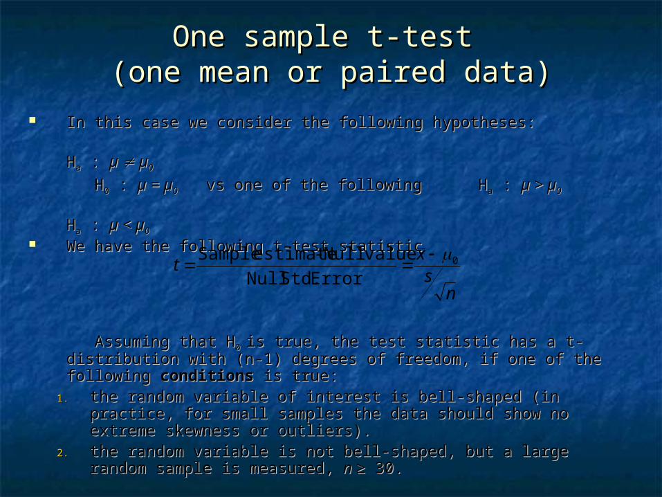
In this case we consider the following hypotheses: In this case we consider the following hypotheses:

HHaa : : µ µ µ µ00

HH00 : : µ = µµ = µ00 vs one of the following H vs one of the following Haa : : µ > µµ > µ00

HHaa : : µ < µµ < µ00

We have the following t-test statisticWe have the following t-test statistic

Assuming that HAssuming that H0 0 is true, the test statistic has a t-distribution is true, the test statistic has a t-distribution with (n-1) degrees of freedom, if one of the following with (n-1) degrees of freedom, if one of the following conditionsconditions is true: is true:

1.1. the random variable of interest is bell-shaped (in practice, the random variable of interest is bell-shaped (in practice, for small samples the data should show no extreme for small samples the data should show no extreme skewness or outliers).skewness or outliers).

2.2. the random variable is not bell-shaped, but a large random the random variable is not bell-shaped, but a large random sample is measured, sample is measured, n n ≥ 30.≥ 30.

nsx

t 0

Error Std. Null

valueNull -estimate Sample

One sample t-test One sample t-test (one mean or paired data)(one mean or paired data)

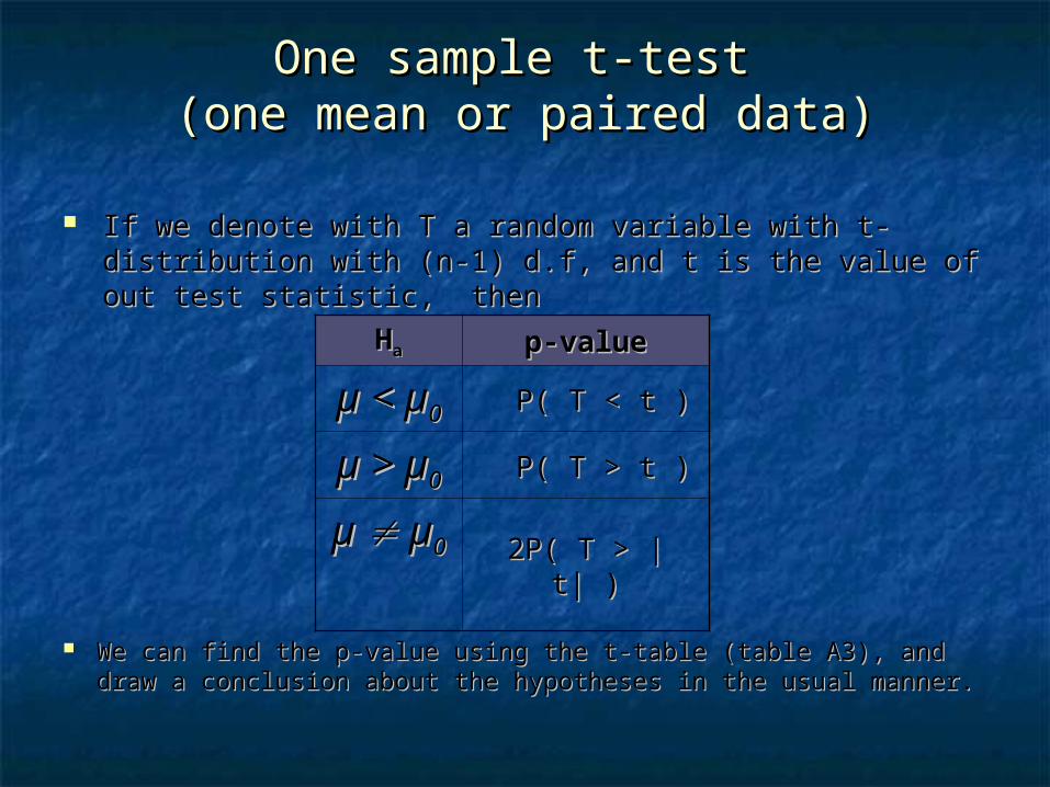
If we denote with T a random variable with t-distribution If we denote with T a random variable with t-distribution with (n-1) d.f, and t is the value of out test statistic, thenwith (n-1) d.f, and t is the value of out test statistic, then

HHaa p-valuep-value

µ < µ < µµ00

P( T < t ) P( T < t )

µ > µ > µµ00

P( T > t )P( T > t )

µ µ µ µ002P( T > |t| )2P( T > |t| )

We can find the p-value using the t-table (table A3), and draw We can find the p-value using the t-table (table A3), and draw a conclusion about the hypotheses in the usual manner. a conclusion about the hypotheses in the usual manner.

Two-Sample t-test Two-Sample t-test (difference between two means).(difference between two means).

There are two populations (Population 1 and 2) of interest having There are two populations (Population 1 and 2) of interest having unknown means unknown means µµ1 1 and µ and µ22 respectively. In this case we consider respectively. In this case we consider the following hypotheses:the following hypotheses:

HHaa : : µµ1 1 - µ- µ22 < < 00 HH00 : : µµ1 1 - µ- µ22 = = 0 0 (i.e. no difference) vs one of the following (i.e. no difference) vs one of the following HHaa : : µµ1 1 - µ- µ22 > >

0 0 HHaa : : µµ1 1 - µ- µ22 00 We have the following t-test statisticWe have the following t-test statistic

Assuming HAssuming H0 0 is true, the test statistic has a t-distribution with is true, the test statistic has a t-distribution with approximate d.f. equal to the minimum of napproximate d.f. equal to the minimum of n11-1 and n-1 and n22-1-1 if the if the following following conditions conditions are true:are true:

1.1. The two samples are independent.The two samples are independent.2.2. Each sample is either coming from a bell shaped population or the Each sample is either coming from a bell shaped population or the

sample size is ≥30.sample size is ≥30. Using the appropriate d.f, we can get the p-value from table A.3 in Using the appropriate d.f, we can get the p-value from table A.3 in

the same way as in the one-mean case.the same way as in the one-mean case.

2

2

1

1

2122

0)(

ns

ns

xxt

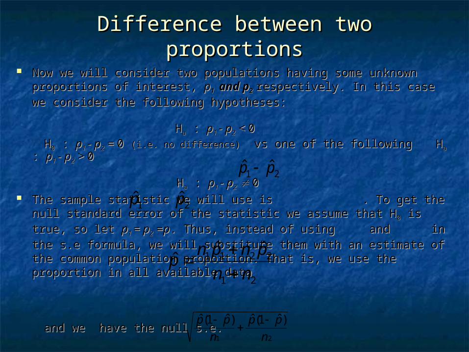
Now we will consider two populations having some unknown Now we will consider two populations having some unknown proportions of interest, proportions of interest, pp1 1 and p and p22 respectively. In this case we respectively. In this case we consider the following hypotheses:consider the following hypotheses:

HHaa : : pp1 1 - p- p22 < < 00 HH00 : : pp1 1 - p- p22 = = 0 0 (i.e. no difference)(i.e. no difference) vs one of the following vs one of the following HHaa : : pp1 1 - p- p22

> > 0 0 HHaa : : pp1 1 - p- p22 00 The sample statistic we will use is . To get the null The sample statistic we will use is . To get the null

standard error of the statistic we assume that Hstandard error of the statistic we assume that H00 is true, so let is true, so let pp1 1

= p= p22 ==pp. Thus, instead of using and in the s.e formula, we . Thus, instead of using and in the s.e formula, we will substitute them with an estimate of the common population will substitute them with an estimate of the common population proportion. That is, we use the proportion in all available dataproportion. That is, we use the proportion in all available data

and we have the null s.e.and we have the null s.e.

Difference between two proportionsDifference between two proportions

1p̂

21 ˆˆ pp

2p̂

21

2211 ˆˆˆ

nn

pnpnp

21

)ˆ1(ˆ)ˆ1(ˆ

n

pp

n

pp

Difference between two Difference between two proportionsproportions

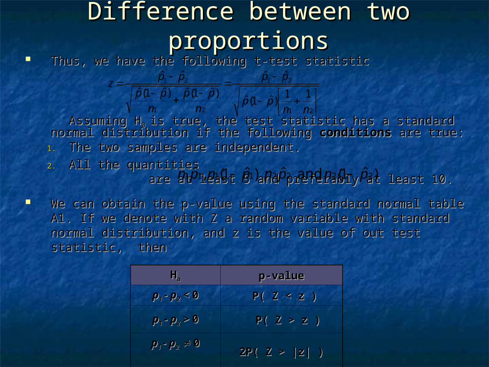
Thus, we have the following t-test statisticThus, we have the following t-test statistic

Assuming HAssuming H0 0 is true, the test statistic has a standard normal is true, the test statistic has a standard normal distribution if the following distribution if the following conditions conditions are true:are true:

1.1. The two samples are independent.The two samples are independent.

2.2. All the quantities are at All the quantities are at least 5 and preferably at least 10.least 5 and preferably at least 10.

We can obtain the p-value using the standard normal table We can obtain the p-value using the standard normal table A1. If we denote with Z a random variable with standard A1. If we denote with Z a random variable with standard normal distribution, and z is the value of out test statistic, normal distribution, and z is the value of out test statistic, thenthen

21

21

21

21

11)ˆ1(ˆ

ˆˆ

)ˆ1(ˆ)ˆ1(ˆ

ˆˆ

nnpp

pp

npp

npp

ppz

)ˆ1( and ˆ),ˆ1(,ˆ 22221111 pnpnpnpn

HHaa p-valuep-value

pp1 1 - p- p22 < < 00 P( Z < z ) P( Z < z )

pp1 1 - p- p22 > > 00 P( Z > z )P( Z > z )

pp1 1 - p- p22 002P( Z > |z| )2P( Z > |z| )

Table For Hypothesis Table For Hypothesis TestingTesting

TypeType ParameteParameterr

StatistiStatisticc

Null Std. ErrorNull Std. Error Test Test StatisticStatistic

One Mean (or One Mean (or Paired mean)Paired mean) µ or µµ or µdd

or or or or tt

df = n-1df = n-1

Difference Difference Between Between MeansMeans

µµ11- µ- µ22

ttdf=min(ndf=min(n11-1,n-1,n22--1)1)

One One ProportionProportion pp

zz

Difference Difference Between Between ProportionsProportions

pp11-p-p22 zz

x dn

s

n

sd

21 xx 2

2

1

122

n

s

n

s

p̂

21 ˆˆ pp

n

pp oo )1(

21

21

)ˆ1(ˆ)ˆ1(ˆ

ˆˆ

npp

npp

pp

p̂

=

21

2211 ˆˆ

nn

pnpn

.

= This is the overall proportion-like if we had one big sample!

Detailed Example 1Detailed Example 1

A box of corn flakes is advertised as A box of corn flakes is advertised as containing containing 16 oz.16 oz. of cereal. John works for of cereal. John works for consumer reports and is interesting in consumer reports and is interesting in verifying the companies claim. He suspects verifying the companies claim. He suspects that the average amount of cereal is that the average amount of cereal is lessless than 16oz. He takes a random sample of than 16oz. He takes a random sample of 100 100 boxes of cereal and records the weight boxes of cereal and records the weight of each box. The sample mean is of each box. The sample mean is 15.7oz15.7oz and the sample standard deviation is and the sample standard deviation is 1.2oz.1.2oz.

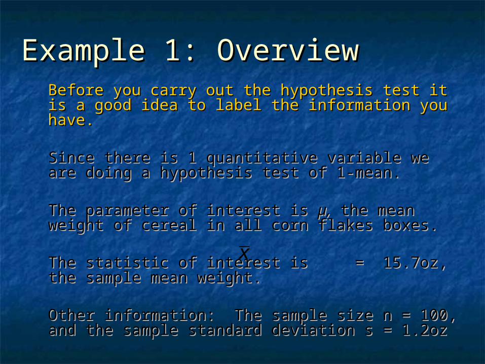
Example 1: OverviewExample 1: OverviewBefore you carry out the hypothesis test it is a Before you carry out the hypothesis test it is a good idea to label the information you have.good idea to label the information you have.

Since there is 1 quantitative variable we are Since there is 1 quantitative variable we are doing a hypothesis test of 1-mean. doing a hypothesis test of 1-mean.

The parameter of interest is The parameter of interest is µ,µ, the mean weight the mean weight of cereal in all corn flakes boxes. of cereal in all corn flakes boxes.

The statistic of interest is = 15.7oz, the The statistic of interest is = 15.7oz, the sample mean weight.sample mean weight.

Other information: The sample size n = 100, and Other information: The sample size n = 100, and the sample standard deviation s = 1.2ozthe sample standard deviation s = 1.2oz

x

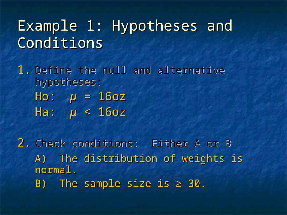
Example 1: Hypotheses and Example 1: Hypotheses and ConditionsConditions

1.1. Define the null and alternative Define the null and alternative hypotheses:hypotheses:

Ho: Ho: µµ = 16oz = 16ozHa: Ha: μμ < 16oz < 16oz

2.2. Check conditions: Either A or BCheck conditions: Either A or B

A) The distribution of weights is normal.A) The distribution of weights is normal.B) The sample size is ≥ 30.B) The sample size is ≥ 30.

Example 1: Test Statistic and P-Example 1: Test Statistic and P-ValueValue

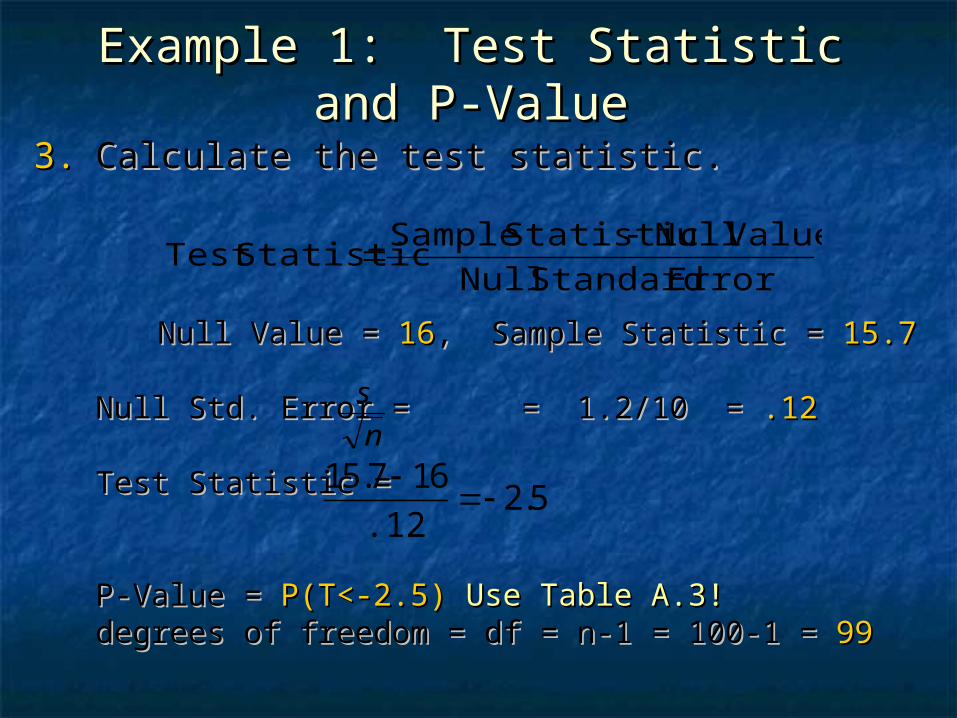
3.3. Calculate the test statistic.Calculate the test statistic.

Null Value = Null Value = 1616, Sample Statistic = , Sample Statistic = 15.715.7

Null Std. Error = = 1.2/10 = Null Std. Error = = 1.2/10 = .12.12

Test Statistic = Test Statistic =

P-Value = P-Value = P(T<-2.5)P(T<-2.5) Use Table A.3!Use Table A.3!degrees of freedom = df = n-1 = 100-1 = degrees of freedom = df = n-1 = 100-1 = 9999

Error Standard Null

Value NullStatistic Sample StatisticTest

n

s

5.2.12

617.51

Example 1: P-value & ConclusionExample 1: P-value & Conclusion

T-Distribution, df = 99

P-Value = P(T<-2.5)

-4 -2 0 2 4

T

0.0

0.1

0.2

0.3

Densi

ty

Table A.3 gives the one-sided p-values for t-tests. For 2-sided hypothesis tests make sure you multiply the p-value by 2!

Look up the absolute value of the test statistic and df in the table. If they do not have the exact test statistic, then take your best guess OR use the next smallest test statistic. Using the next larger and next smallest value for t-statistic on the table you can get an interval for the p-value.

In our case, df = 99 and t-statistic = -2.5. Since 2.5 is not in the table we can use 2.33, and 90 df (since 99 is not in the table). We get that the p-value is less than .011.

The p-value is < .05 so we REJECT the null hypothesis and we conclude that the average weight IS less than 16oz.

Detailed Example 2Detailed Example 2

A potential presidential candidate in 2002 A potential presidential candidate in 2002 election wished to know if men and women election wished to know if men and women had equal preferences for her candidacy had equal preferences for her candidacy versus this not being the case (she versus this not being the case (she suspected that men were more likely to favor suspected that men were more likely to favor her). Her pollster polled a random sample of her). Her pollster polled a random sample of 400 men and 400 women, with the following 400 men and 400 women, with the following results.results.Preference: Would vote for her?Preference: Would vote for her? NoNo Yes Yes TotalTotalMenMen 164164 236236 400400WomenWomen 180180 220220 400400Total Total 344344 556556 800800

Example 2: OverviewExample 2: Overview

Here there are 2 categorical variables, both with 2 Here there are 2 categorical variables, both with 2 levels so we are interested in a test of 2-proportions! levels so we are interested in a test of 2-proportions!

Is the proportion of men who favor the candidate Is the proportion of men who favor the candidate greater than the proportion of women who favor the greater than the proportion of women who favor the candidate?candidate?

The parameter of interest is pThe parameter of interest is pmm-p-pww..

The sample statistic of interest is =.59-.55 = The sample statistic of interest is =.59-.55 = .04.04

wm pp ˆˆ

1.1. Calculate the null and alternative hypotheses:Calculate the null and alternative hypotheses:

Ho: Ho: ppmm = p = pff or or ppmm-p-pff = 0 = 0

Ha: Ha: ppmm > > ppff oror ppmm-p-pff > 0 > 0

Let’s denote with Let’s denote with ppmm with with pp11 and and ppff with with pp22..

2.2. Check the conditions:Check the conditions:

All quantities, and All quantities, and are greater than or equal to 10. are greater than or equal to 10.

)ˆ1(,ˆ 1111 pnpn )ˆ1(,ˆ 2222 pnpn

Example 2:Example 2:

Example 2: Test Statistic and P-Example 2: Test Statistic and P-ValueValue

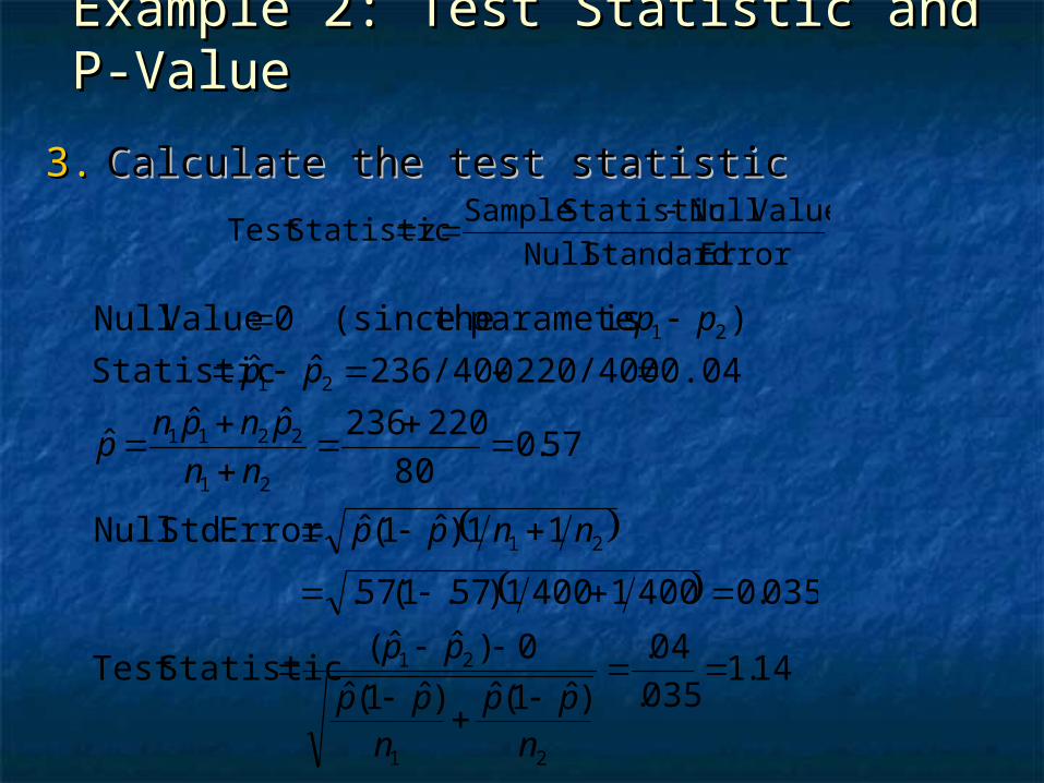
3.3. Calculate the test statisticCalculate the test statistic

Error Standard Null

Value NullStatistic Sample zStatisticTest

14.1035.

04.

)ˆ1(ˆ)ˆ1(ˆ

0)ˆˆ( StatisticTest

035.040014001)57.1(57.

11)ˆ1(ˆ Error Std. Null

57.080

220236ˆˆˆ

0.04 220/400– 236/400ˆˆStatistic

) is paramete the(since 0 Value Null

21

21

21

21

2211

21

21

npp

npp

pp

nnpp

nn

pnpnp

pp

pp

Example 2: P-Value and Example 2: P-Value and ConclusionConclusion

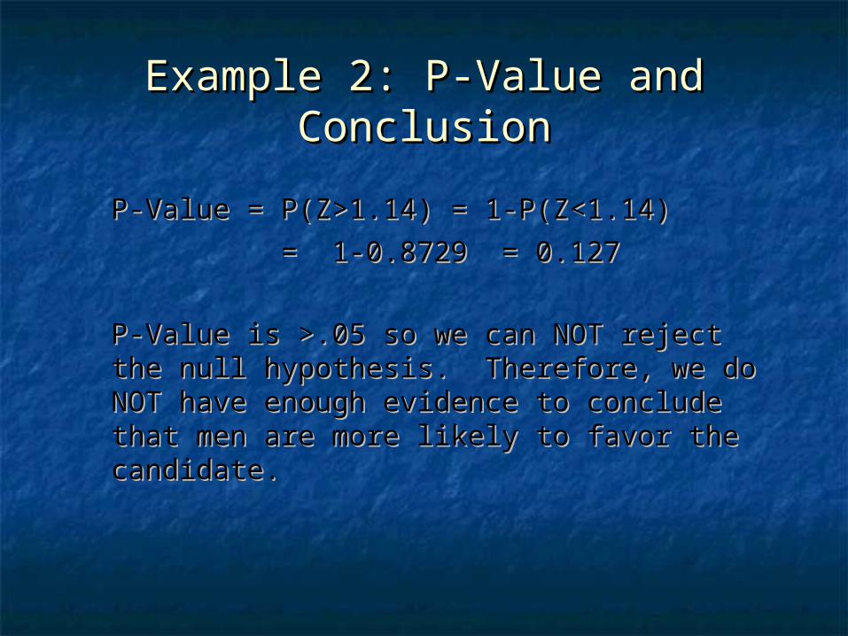
P-Value = P(Z>1.14) = 1-P(Z<1.14)P-Value = P(Z>1.14) = 1-P(Z<1.14)

= 1-0.8729 = 0.127= 1-0.8729 = 0.127

P-Value is >.05 so we can NOT reject the null P-Value is >.05 so we can NOT reject the null hypothesis. Therefore, we do NOT have hypothesis. Therefore, we do NOT have enough evidence to conclude that men are enough evidence to conclude that men are more likely to favor the candidate.more likely to favor the candidate.

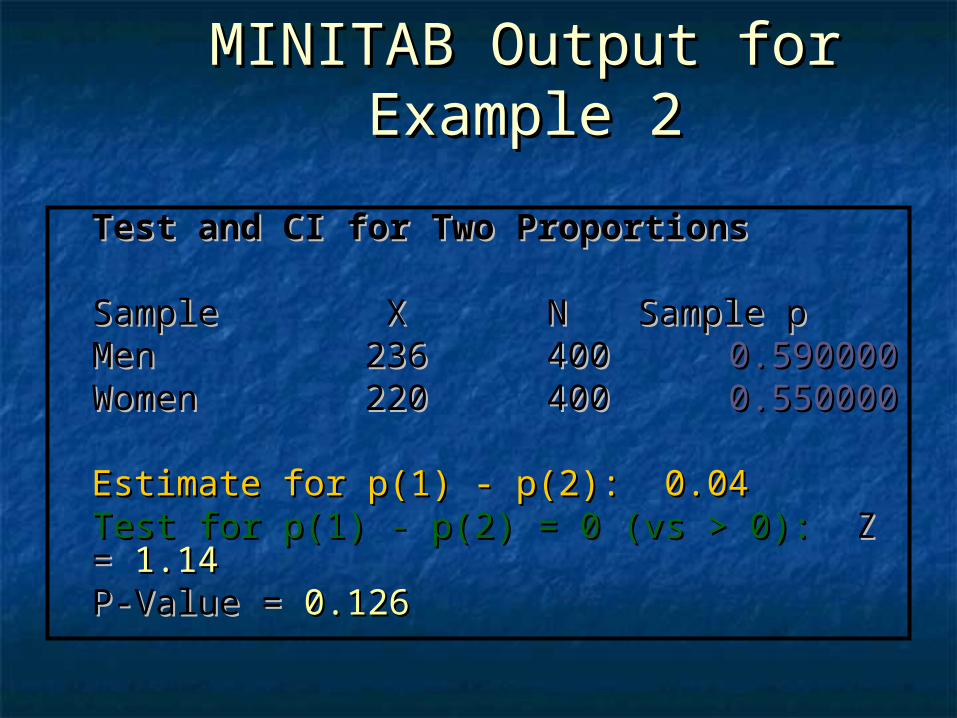
MINITAB Output for Example MINITAB Output for Example 22

Test and CI for Two ProportionsTest and CI for Two Proportions

Sample Sample X X N N Sample pSample pMen Men 236 236 400 400 0.5900000.590000Women Women 220 220 400 400 0.5500000.550000

Estimate for p(1) - p(2): 0.04Estimate for p(1) - p(2): 0.04Test forTest for p(1) - p(2) = 0 (vs > 0):p(1) - p(2) = 0 (vs > 0): Z = Z = 1.14 1.14 P-Value = P-Value = 0.1260.126

CI’s and Two-sided CI’s and Two-sided AlternativesAlternatives

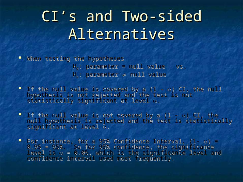
When testing the hypothesesWhen testing the hypotheses HH00: parameter = null value vs. : parameter = null value vs. HHaa: parameter : parameter null value null value

If the null value is covered by a (1 - If the null value is covered by a (1 - ) CI, the null hypothesis is ) CI, the null hypothesis is not rejected and the test is not statistically significant at level not rejected and the test is not statistically significant at level ..

If the null value is not covered by a (1 - If the null value is not covered by a (1 - ) CI, the null ) CI, the null hypothesis is rejected and the test is statistically significant at hypothesis is rejected and the test is statistically significant at level level ..

For instance, for a 95% Confidence Interval, (1- For instance, for a 95% Confidence Interval, (1- ) = 0.95 = ) = 0.95 = 95%. So for 95% confidence, the significance level is 95%. So for 95% confidence, the significance level is = 0.05, = 0.05, which is the significance level and confidence interval used which is the significance level and confidence interval used most frequently.most frequently.

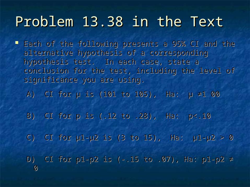
Problem 13.38 in the TextProblem 13.38 in the Text Each of the following presents a 95% CI and the Each of the following presents a 95% CI and the

alternative hypothesis of a corresponding alternative hypothesis of a corresponding hypothesis test. In each case, state a conclusion hypothesis test. In each case, state a conclusion for the test, including the level of significance you for the test, including the level of significance you are using.are using.

A) CI for µ is (101 to 105), Ha: µ ≠1 00A) CI for µ is (101 to 105), Ha: µ ≠1 00

B) CI for p is (.12 to .28), Ha: p<.10B) CI for p is (.12 to .28), Ha: p<.10

C) CI for µ1-µ2 is (3 to 15), Ha: µ1-µ2 > 0C) CI for µ1-µ2 is (3 to 15), Ha: µ1-µ2 > 0

D) CI for p1-p2 is (-.15 to .07), Ha: p1-p2 ≠ 0D) CI for p1-p2 is (-.15 to .07), Ha: p1-p2 ≠ 0

Possible Errors, Power and Possible Errors, Power and Sample Size Considerations Sample Size Considerations

When we are testing a hypothesis two out four possible decisions When we are testing a hypothesis two out four possible decisions lead to an error.lead to an error.Type I errorType I error - We reject H - We reject H00 when it is true when it is trueType II errorType II error- We fail to reject H- We fail to reject H00 when H when Haa is true. is true.

There is an inverse relationship between the probabilities of the two There is an inverse relationship between the probabilities of the two types of errors. Increase in the probability of type I error leads to types of errors. Increase in the probability of type I error leads to decrease in the probability of type II error and vice versa.decrease in the probability of type II error and vice versa.

When the alternative hypothesis is true, the probability of making the When the alternative hypothesis is true, the probability of making the correct decision is called correct decision is called powerpower of the test. of the test.

The power increases when the sample size increased. Can you see The power increases when the sample size increased. Can you see why?why?

The power increases when the difference between the true population The power increases when the difference between the true population parameter value and the null value increases. Can you see why?parameter value and the null value increases. Can you see why?

The hypothesis test may have very low power because of small data The hypothesis test may have very low power because of small data set.set.

We should also be careful in cases our conclusions are based on We should also be careful in cases our conclusions are based on extremely large samples, since in cases like that even a weak extremely large samples, since in cases like that even a weak relationship (or a small difference) can be statistically significant.relationship (or a small difference) can be statistically significant.