NST 1B Experimental PsychologyStatistics practical 3

Difference tests (2):nonparametric

Rudolf Cardinal & Mike Aitken10 / 11 February 2005; Department of Experimental Psychology

University of Cambridge

Slides atpobox.com/~rudolf/psychology

These slides are on the web.No need to scribble frantically.

pobox.com/~rudolf/psychology

Nonparametric tests

Last time, we looked at the t test, a parametric test — it madeassumptions about parameters of the underlying populations (such asthe distribution — e.g. assuming that the data are normallydistributed).

If these assumptions are violated:(a) we could transform the data to fit the assumptions better

(NOT covered at Part 1B level)or (b) we could use a nonparametric (‘distribution-free’) test that doesn’t make the same assumptions.

In general, if the assumptions of parametric tests are met, they are themost powerful. If not, we may need to use nonparametric tests. Theymay, for example, answer questions about medians rather thanmeans. We’ll look at some nonparametric tests now that assume onlythat the data are measured on at least an ordinal scale.

The median

The median is the value at or below which 50% of the scores fallwhen the data are arranged in numerical order.

(Can also be referred to as the 50th centile.)

If n is odd, it’s the middle value (here, 17):

If n is even, it’s the mean of the two middle values (here, 17.5):

10 11 12 14 15 15 17 17 18 18 18 19 19 20 23

10 11 12 14 15 15 17 17 18 18 18 19 19 20 21 23

the two middle valuesThe median is (17+18) ÷ 2 = 17.5

The median

The median is the value at or below which 50% of the scores fallwhen the data are arranged in numerical order.

(Can also be referred to as the 50th centile.)

Medians are less affected by outliers than means

Ranking removes ‘distribution’ information

How to rank data

Suppose we have ten measurements (e.g. test scores) and want to rankthem. First, place them in ascending numerical order:

5 8 9 12 12 15 16 16 16 17

Then start assigning them ranks. When you come to a tie, give each valuethe mean of the ranks they’re tied for — for example, the 12s are tied forranks 4 and 5, so they get the rank 4.5; the 16s are tied for ranks 7, 8, and9, so they get the rank 8:

X: 5 8 9 12 12 15 16 16 16 17rank: 1 2 3 4.5 4.5 6 8 8 8 10

Nonparametric correlationWe’ve already seen this.

rs: Spearman’s correlation coefficient for ranked data

We met this in the first statistics practical. It’s a nonparametricversion of correlation. You can use it when you obtain ranked data,or when you want to do significance tests on r but your data are notnormally distributed (violating an assumption of the parametric ttest that’s based on Pearson’s r).

• Rank the X values.• Rank the Y values.• Correlate the X ranks with the Y ranks. (You do this inthe normal way for calculating r, but you call the resultrs.)• To ask whether the correlation is ‘significant’, use thetable of critical values of Spearman’s rs in the Tables andFormulae booklet.

Nonparametric difference tests

Two unrelated samples: the Mann–Whitney U test

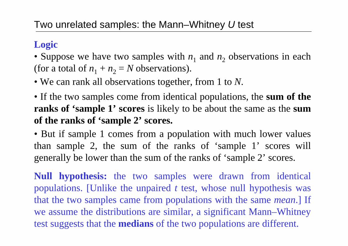
Null hypothesis: the two samples were drawn from identicalpopulations. [Unlike the unpaired t test, whose null hypothesis wasthat the two samples came from populations with the same mean.] Ifwe assume the distributions are similar, a significant Mann–Whitneytest suggests that the medians of the two populations are different.

Logic• Suppose we have two samples with n1 and n2 observations in each(for a total of n1 + n2 = N observations).• We can rank all observations together, from 1 to N.

• If the two samples come from identical populations, the sum of theranks of ‘sample 1’ scores is likely to be about the same as the sumof the ranks of ‘sample 2’ scores.• But if sample 1 comes from a population with much lower valuesthan sample 2, the sum of the ranks of ‘sample 1’ scores willgenerally be lower than the sum of the ranks of ‘sample 2’ scores.

Calculating the Mann–Whitney U statistic

1. Call the smaller group ‘group 1’, and the larger group ‘group 2’, so n1 < n2.(If n1

= n2, ignore this step.)2. Calculate the sum of the ranks of group 1 (= R1) and group 2 (= R2).

3. 2

)1( 1111

+−=

nnRU

4. 2

)1( 2222

+−=

nnRU

5. The Mann–Whitney statistic U is the smaller of U1 and U2.

Check your sums: verify that U1 + U2 = n1n2 and 2

)1)(( 212121

+++=+ nnnnRR .

Calculating the Mann–Whitney U statistic

From the Formula Sheet:

Mann–Whitney U test: EXAMPLE 1

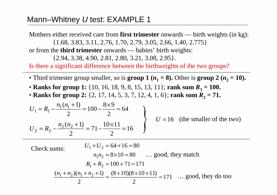
Mothers either received care from first trimester onwards — birth weights (in kg):{1.68, 3.83, 3.11, 2.76, 1.70, 2.79, 3.05, 2.66, 1.40, 2.775}

or from the third trimester onwards — babies’ birth weights:{2.94, 3.38, 4.90, 2.81, 2.80, 3.21, 3.08, 2.95}.

Is there a significant difference between the birthweights of the two groups?

• Third trimester group smaller, so is group 1 (n1 = 8). Other is group 2 (n2 = 10).

642

98100

2

)1( 1111 =×−=+−= nn

RU

162

111071

2

)1( 2222 =×−=+−= nn

RU

1712

)11108)(108(

2

)1)((

17171100

80108

801664

2121

21

21

21

=+++=+++=+=+

=×==+=+

nnnn

RR

nn

UU

16=U (the smaller of the two)

Check sums:… good, they match

… good, they do too

• Ranks for group 1: {10, 16, 18, 9, 8, 15, 13, 11}; rank sum R1 = 100.• Ranks for group 2: {2, 17, 14, 5, 3, 7, 12, 4, 1, 6}; rank sum R2 = 71.

Distribution of the Mann–Whitney U statistic (if H0 is true)

A discrete (stepwise) distribution,rather than the continuousdistributions we’ve looked at before.

Determining a significance level (p value) from U

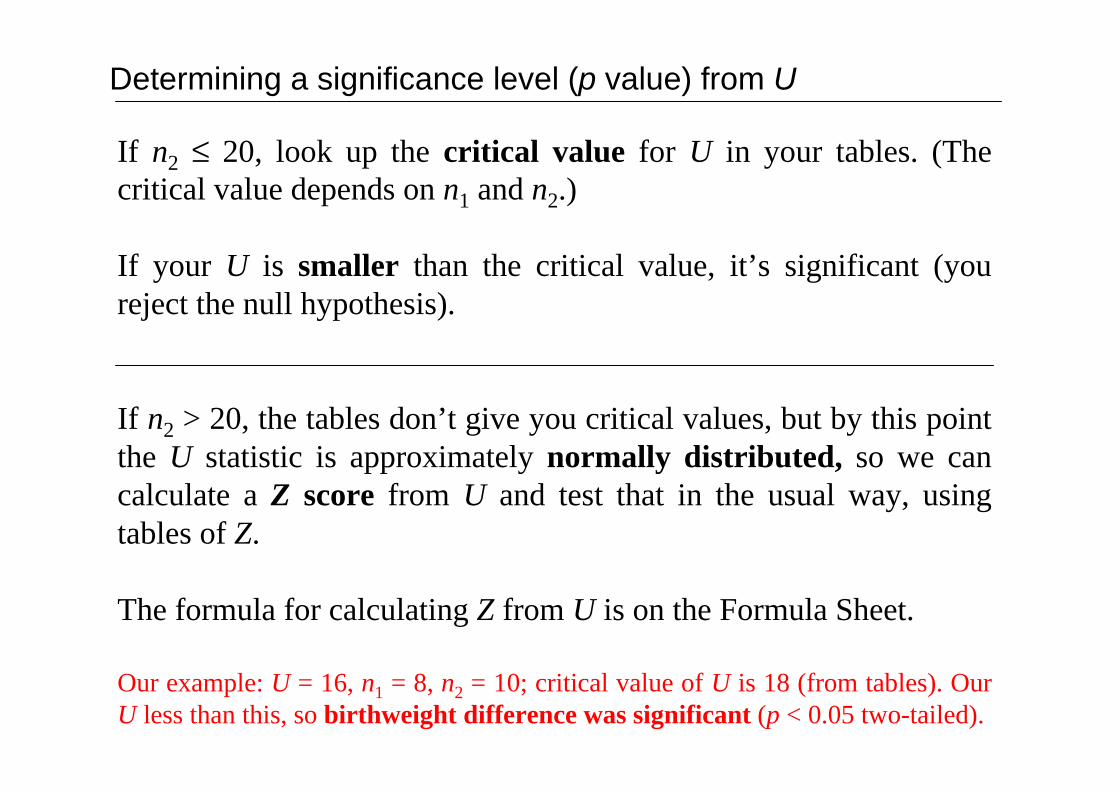
If n2 ≤ 20, look up the critical value for U in your tables. (Thecritical value depends on n1 and n2.)

If your U is smaller than the critical value, it’s significant (youreject the null hypothesis).

If n2 > 20, the tables don’t give you critical values, but by this pointthe U statistic is approximately normally distributed, so we cancalculate a Z score from U and test that in the usual way, usingtables of Z.

The formula for calculating Z from U is on the Formula Sheet.

Our example: U = 16, n1 = 8, n2 = 10; critical value of U is 18 (from tables). OurU less than this, so birthweight difference was significant (p < 0.05 two-tailed).

Mann–Whitney U test: EXAMPLE 2 (a)

Transfer along a continuum practical (a previous year’s data, I’m afraid).Different groups of subjects were trained with {1 or 3} blocks of {easy or hard}discriminations before being tested on similar discriminations. Here are the testscores for the 3-block groups (high = good). Is there an effect of training difficulty?You could use either an unpaired t test or a Mann–Whitney U test; try the latter.

Mann–Whitney U test: EXAMPLE 2 (b)

Last year’s (2003) data465

2

)11515)(1515(

2

)1)((

4655.1725.292

2251515

2255.525.172

2121

21

21

21

=+++=+++=+=+

=×==+=+

nnnn

RR

nn

UU

• Both groups same size. Arbitrarily, call the Easy group ‘group 1’ (n1 = 15). Hardgroup is ‘group 2’ (n2 = 15).• Rank sum R1 = 5.5 + 7 + … + 30 = 292.5• Rank sum R2 = 1 + 2 + … + 25 = 172.5

5.522

16155.172

2

)1( 2222 =×−=+−= nn

RU

Check sums:… good, they match

… good, they do too

5.1722

16155.292

2

)1( 1111 =×−=+−= nn

RU5.52=U (the smaller of the two)

Critical U (n1 = n2 = 15) for α = 0.05two-tailed is 65. So significant.

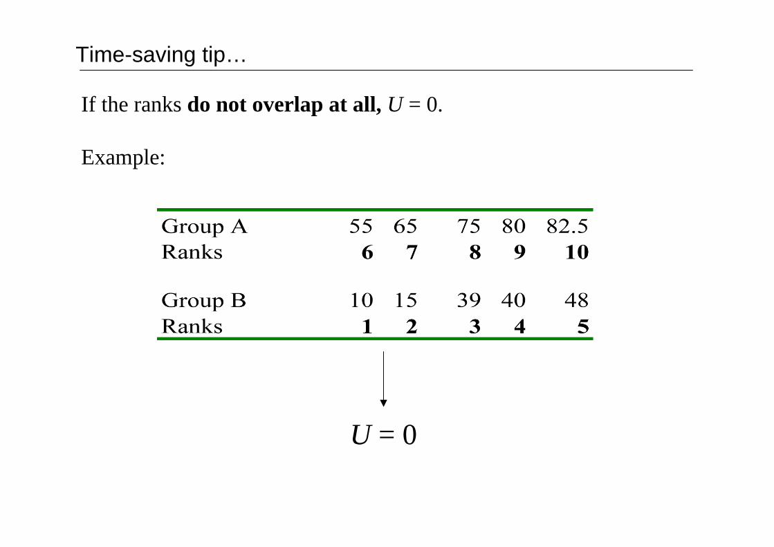
Time-saving tip…

If the ranks do not overlap at all, U = 0.

Example:

U = 0

If you find a significant difference…

If you conduct a Mann–Whitney test and find a significantdifference, which group had the larger median and which grouphad the smaller median?

Here, U = 2. Significant (critical U = 3, α = 0.05 two-tailed).

Group 1 has a significantly larger median (even though the ranksums convey the opposite impression).

You have to calculate the medians. But this is quick.

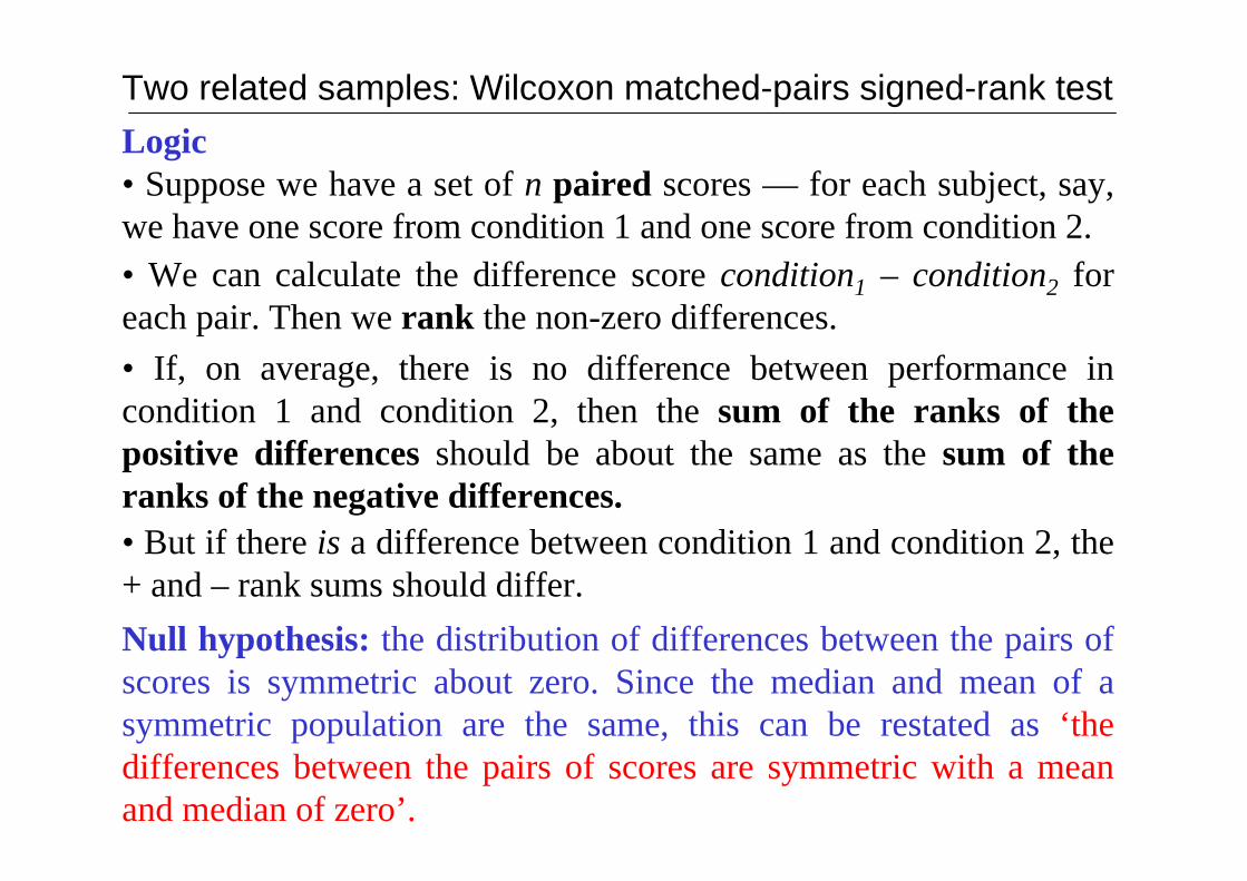
Two related samples: Wilcoxon matched-pairs signed-rank test

Null hypothesis: the distribution of differences between the pairs ofscores is symmetric about zero. Since the median and mean of asymmetric population are the same, this can be restated as ‘thedifferences between the pairs of scores are symmetric with a meanand median of zero’.

Logic• Suppose we have a set of n paired scores — for each subject, say,we have one score from condition 1 and one score from condition 2.• We can calculate the difference score condition1 – condition2 foreach pair. Then we rank the non-zero differences.

• If, on average, there is no difference between performance incondition 1 and condition 2, then the sum of the ranks of thepositive differences should be about the same as the sum of theranks of the negative differences.• But if there is a difference between condition 1 and condition 2, the+ and – rank sums should differ.

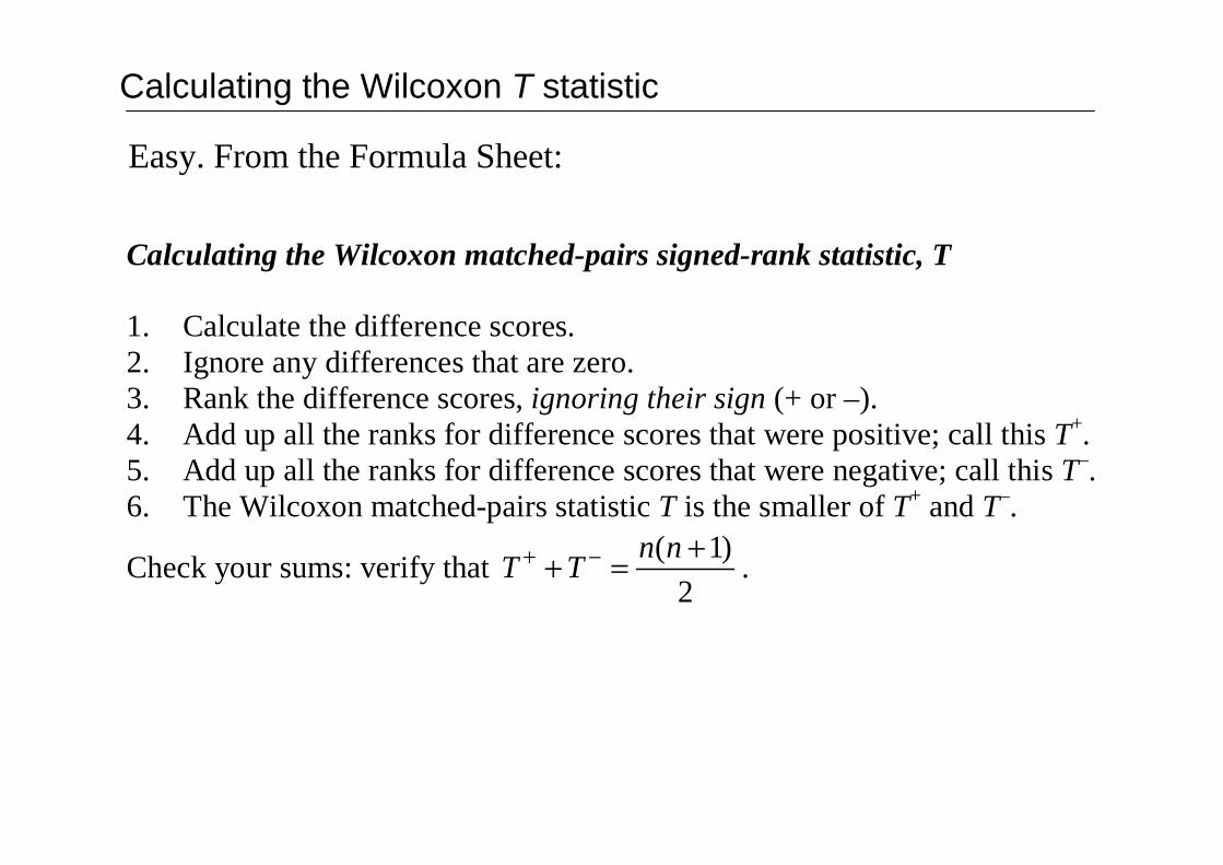
Calculating the Wilcoxon T statistic

Calculating the Wilcoxon matched-pairs signed-rank statistic, T

1. Calculate the difference scores.2. Ignore any differences that are zero.3. Rank the difference scores, ignoring their sign (+ or –).4. Add up all the ranks for difference scores that were positive; call this T+.5. Add up all the ranks for difference scores that were negative; call this T–.6. The Wilcoxon matched-pairs statistic T is the smaller of T+ and T–.

Check your sums: verify that 2

)1( +=+ −+ nnTT .

Easy. From the Formula Sheet:

Wilcoxon matched-pairs signed-rank test: EXAMPLE 1

Measure blood pressure (BP1). Make subjects run a lot. Measure blood pressureagain (BP2) in the same subjects. Has their blood pressure changed?

Sum of positive ranks T+ = 5 + 4 + 2 + 7 + 1 + 8 = 27Sum of negative ranks T– = 6 + 3 = 9

362

98

2

)1(

36927

=×=+=+=+ −+

nn

TT

… good, they matchCheck sums:

Wilcoxon T = the smaller of T+ and T– = 9. And n = 8.

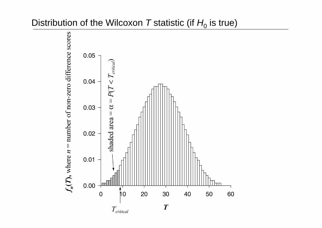
Distribution of the Wilcoxon T statistic (if H0 is true)

Determining a significance level (p value) from T

If n ≤ 25, look up the critical value for T in your tables. (Thecritical value depends on n.)

If your T is smaller than the critical value, it’s significant (youreject the null hypothesis).

If n > 25, the tables don’t give you critical values, but by this pointthe T statistic is approximately normally distributed, so we cancalculate a Z score from T and test that in the usual way, usingtables of Z.

The formula for calculating Z from T is on the Formula Sheet.

In our example, T = 9 and n = 8. Critical value of T is 4 (for α = 0.05 two-tailed);since our T is not smaller than this, the BP difference was not significant.

Wilcoxon matched-pairs signed-rank test: EXAMPLE 2 (a)Proactive interference practical (subset of a previous year’s data, I’m afraid).Subjects hear and repeat trigram (e.g. CXJ), perform distractor task, recall trigram.Compare trials 9 & 10 (after many similar trigrams) with trials 11 & 12 (after shiftto new type of trigram, e.g. 925). Is there ‘release’ from proactive interference?Note very non-normal difference scores; parametric test unsuitable.

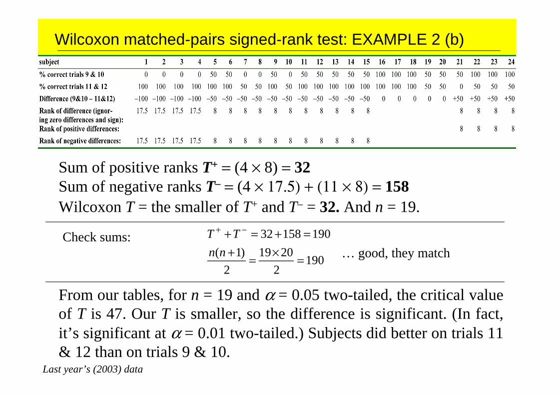
Wilcoxon matched-pairs signed-rank test: EXAMPLE 2 (b)

Last year’s (2003) data

Sum of positive ranks T+ = (4 × 8) = 32Sum of negative ranks T– = (4 × 17.5) + (11 × 8) = 158

1902

2019

2

)1(

19015832

=×=+=+=+ −+

nn

TT

… good, they matchCheck sums:

Wilcoxon T = the smaller of T+ and T– = 32. And n = 19.

From our tables, for n = 19 and α = 0.05 two-tailed, the critical valueof T is 47. Our T is smaller, so the difference is significant. (In fact,it’s significant at α = 0.01 two-tailed.) Subjects did better on trials 11& 12 than on trials 9 & 10.

One sample: Wilcoxon signed-rank test with only one sample

Very easy.Null hypothesis: the median is equal to M.

For each score x, calculate a difference score (x – M). Then proceedas for the two-sample Wilcoxon test using these difference scores.

(Logic: if the median is M, then the sum of the ranks of the positive differences— from scores where x > M — should be the same as the sum of the ranks of thenegative differences — from scores where x < M. If the median isn’t M, then thetwo rank sums should differ.)

Parametric test Equivalent nonparametric testTwo-sample unpaired t test Mann–Whitney U testTwo-sample paired t test Wilcoxon signed-rank test with matched pairsOne-sample t test Wilcoxon signed-rank test, pairing data with a fixed value

Comparison of parametric and non-parametric tests