monte carlo simulations of absorption and fluorescence spectra in ellipsoidal nanocavities

Monte Carlo Simulations of Absorption and Fluorescence Spectra in EllipsoidalNanocavities

J. A. Gomez and Ward H. Thompson*Department of Chemistry, UniVersity of Kansas, Lawrence, Kansas 66045

ReceiVed: February 29, 2004; In Final Form: June 18, 2004

The absorption and fluorescence spectra of a model solute molecule dissolved in a CH3I solvent confined innanoscale ellipsoidal cavities have been simulated for solutions with densities equal to 1.4, 2.0, and 2.2 g/cm3.The model solute is a diatomic molecule with an electronic charge-transfer transition. Monte Carlo simulationshave been performed for solutions confined in hydrophobic prolate and oblate ellipsoidal cavities of varyingsize. The results of the absorption and fluorescence spectra are compared with previous simulations of confinedsolvents in spherical cavities. The solute and solvent molecule probability density distributions have beencalculated and are used to interpret the spectra. An umbrella sampling approach is used to obtain accurateresults for the solute probability distributions.

1. Introduction

Advances in synthetic techniques have made it possible togenerate confined solvent systems with a wide variety ofproperties.1-6 Among the confining frameworks that have beenthe subject of recent study are sol-gels,1,7-12 reversemicelles,2,13-18 zeolites,19 proteins, and supramolecular as-semblies.3 These systems are of interest for a variety of potentialapplications including catalysis, sensors, and separations as wellas understanding systems occurring in nature.21 However, theseconfining structures are extremely diverse, varying widely indimensionality (e.g., cavities versus pores), size, shape, surfaceroughness, surface flexibility, and chemical functionality, andthe chemical dynamics is frequently complex. Thus, developinggeneral principles for designing confining frameworks that willserve a specific purpose (e.g., a microporous catalyst) is not asimple task. Simulations provide an important complement toexperimental measurements since the cavity or pore character-istics can be explicitly controlled and the effects of each propertyon chemistry occurring in the confined solvent determined.6,15-26

Recently, we have simulated the charge-transfer spectra25 andtime-dependent fluorescence26 (TDF) of a model dye moleculeinside spherical, hydrophobic nanocavities as a function of cavitysize. These processes are interesting both for comparisons withexperimental measurements and for insights into charge-transferreactions (e.g., electron or proton transfer) that involve similarsolvent reorientational dynamics. In addition, charge transferprocesses are, in general, strongly affected by solvent confine-ment since they are intimately coupled to the solvent dynamics.Our previous simulations found that the distribution of solutepositions inside the cavity is an important variable that impactsboth steady-state spectra25 and time-dependent fluorescence.26

Specifically, the solute dye molecule has a significantly largerdipole moment in the excited state compared to the ground state.This leads to an excited state solute position distribution that ispeaked in the cavity interior (a fully solvated solute) and aground state position distribution peaked near the cavity wall(a half-solvated solute). The corresponding fluorescence spectraare therefore sensitive to the changes in effective solvent polaritythat occur upon changing the cavity size, while the absorptionspectra are relatively insensitive to the same changes: the

fluorescence spectra shift consistently to the red (longerwavelength) as the cavity size is increased, while the absorptionspectra are essentially unchanged. The difference in ground andexcited-state position distributions led to the prediction thatsolute motion may contribute to the time-dependent fluorescencesignal.25 This prediction was verified using nonequilibriummolecular dynamics simulations.26

In this paper we extend our Monte Carlo simulations of thesteady-state spectra of a dye molecule in spherical nanoscalecavities to ellipsoidal cavities. Thus, we move beyond theconsideration of cavity size to examine the effect of changingcavity shape and, naturally, the breaking of spherical symmetry.We consider both prolate and oblate ellipsoidal cavities ofvarying size (beginning from the spherical case). The solute-solvent system is the same as in previous work25,26 and isoutlined in section 2 along with the extension of the cavitymodel to ellipsoids. The details of the Monte Carlo simulationsincluding the umbrella sampling approach necessary to obtainaccurate solute position distributions are described in section3. The solvent and solute position distributions along with thesteady-state absorption and fluorescence spectra are presentedand discussed in section 4. Finally, some concluding remarksare given in section 5.

2. Interaction Potential

2.1. Potential Form. We have carried out Monte Carlosimulations for a model solute molecule dissolved in a CH3Isolvent confined in ellipsoidal cavities. The solute is a modeldiatomic molecule (denoted as AB), with an electronic charge-transfer transition. The electronic structure of the solute isdescribed in terms of a two valence bond state model withelectronic coupling of only 0.01 eV so that the ground and theexcited states have effectively fixed charges with moleculardipoles of 1.44 and 7.2 D, respectively. The excited state is 2eV higher in energy than the ground state. The CH3I solventmolecules are also considered as diatomic molecules with fixedmolecular dipole equal to 2.6 D.27 The methyl groups in thesolvent are treated as “unified atoms.” Both solute and solventare rigid molecules.

20144 J. Phys. Chem. B2004,108,20144-20154

10.1021/jp049092v CCC: $27.50 © 2004 American Chemical SocietyPublished on Web 08/24/2004

The solute AB interacts with the CH3I solvent moleculesthrough Lennard-Jones and Coulomb potentials. The Lennard-Jones parameters for atoms A and B are the same andindependent of the electronic state. The interactions of the soluteand solvent molecules with the cavity wall involve a Lennard-Jones interaction. A general expression for the total potentialenergy for a system ofN molecules confined in a cavity is givenby

whereni is the number of atoms (or interaction sites) in moleculei, rRiRj denotes the distance between atomsRi and Rj onmoleculesi andj, rRi denotes the position of atomRi with respectto the center of the cavity, andqRi is the charge of atomRi. Thefirst term in eq 1 gives the contribution to the total potentialenergy due to the intermolecular interactions while the secondterm gives the contribution due to the molecule-cavity wallinteractions. The Lennard-Jones potential energy betweenmolecules is given by

whereσRiRj andεRiRj represent, respectively, the Lennard-Jonesdiameter and well-depth parameter. The termsuLJ

ws(rRi) are theLennard-Jones interactions of atoms with the cavity wall andare explained in detail in section 2.2. The model parametersfor solute25 and solvent molecules27 are the same as those usedin previous work25 and are given in Table 1.

2.2. Molecule-Wall Interactions for Ellipsoidal Cavities.A number of previous works17,18,22,23have considered moleculesconfined inside smooth spherical cavities. When moleculesinteract with these cavity walls via a Lennard-Jones interaction,the result is a potential energy that depends only on the distanceof each interaction site in a molecule from the center of thecavity.15,16Due to the spherical symmetry, structural propertiesof molecules need only be examined as a function of radialcoordinates. In this work, we examine the effects of breakingthe spherical symmetry by considering ellipsoidal cavities. Weconsider prolate and oblate ellipsoidal cavities with the walldefined by

wherea andc are the semi-axes of the ellipsoidal cavity (seeFigure 1). A spherical cavity is obtained whena ) c andc >a (c < a) gives a prolate (oblate) ellipsoid.

In the calculation of the Lennard-Jones interaction betweenthe molecules and cavity wall, it is assumed that the regionexterior to the cavity consists of a uniform densityF ofcontinuum sites. The Lennard-Jones parameters for the cavitywall are the same used in previous work:16-18,25σWall ) 2.5 Å,εWall ) 0.46 kcal/mol. The result of this interaction at the sitepositionr inside the cavity is given by the following expression:

where

Here r is the site position relative to the center of the cavityand ro ranges over the regionΩ exterior to the cavity. Notethat the values of the integralsI(r , n) (n ) 6, 12) depend onthe semi-axesa andc. In contrast to the spherical cavity case,there is no closed expression that represents the interactionpotentialuLJ

ws for ellipsoidal cavities. Hence, the integral in eq 5must be solved by numerical methods. Since these are multi-dimensional integrals, appropriate algorithms include Gaussian29

and pseudo-random30 methods. We used a pseudo-randomapproach, which we find to be more stable than Gaussianmethods. In this method, the grid of points over the regionΩis generated with the Diophantine method,30 which is pseudo-random in the sense that the same “random” point distributionis obtained for the same set of initial parameters.

As an example of the numerical calculation of the potentialuLJ

ws with I(r , n), consider an iodine atom interacting with thewall of an ellipsoidal cavity of semi-axesa ) 10 Å andc ) 30Å. The atom-wall interaction energies for this case are shownas a contour plot in Figure 2 as a function of the atomic positionin the plane of symmetry (see Figure 1). It is clear from thisfigure that the potential energy has a deeper well near the cavitywall along the (long) semi-axisc. This example illustrates thatin the model cavity the interaction potentialuLJ

ws is anisotropicaround the center of the ellipsoidal cavity.

The interaction potential must be calculated many millions(or even billions) of times in a Monte Carlo simulation. Torender this tractable, the values of the integralsI(r , n) (n )6,12) are mapped on a plane that contains the main semi-axisas is shown in Figure 1. (The symmetry about the main semi-axisc is used.) In this symmetry plane, the mapping was doneby using radial and angular polar coordinates. In actualcalculations, we employed a very dense mapping: 300 and 200points for the radial and angular coordinates, respectively. From

Figure 1. A prolate ellipsoid is shown with the minor semi-axesaand the major semi-axisc indicated. The bold lines outline the regionin which the interaction potential integrals, eq 5, are mapped.

V(R) ) ∑i)1

N-1

∑j>1

N

∑Ri)1

ni

∑Rj)1

nj [uLJ(rRiRj) +

qRiqRj

rRiRj] + ∑

i)1

N

∑Ri)1

ni

uLJws(rRi

)

(1)

uLJ(rRiRj) ) 4εRiRj[(σRiRj

rRiRj)12

- (σRiRj

rRiRj)6] (2)

(x2 + y2)

a2+ z2

c2) 1 (3)

Figure 2. The interaction energy of an iodine atom with the ellipsoidalcavity wall (a ) 10 Å, c ) 30 Å) is shown as a function of the atomposition in a plane. Thirty contours are shown from-1.69 to 0.0 kcal/mol.

uLJws(r) ) 4FεWall[σWall

12 I(r , 12)- σWall6 I(r , 6)] (4)

I(r , n) ) ∫Ω

d3ro

|r - ro|n(5)

Absorption and Fluorescence Spectra in Ellipsoidal Nanocavities J. Phys. Chem. B, Vol. 108, No. 52, 200420145

this mapping, we performed a two-dimensional linear interpola-tion for computing the values of the integralsI(r , n) at the siteposition r at each Monte Carlo step. With this methodology,the complex integrals in eq 5 only need to be computed oncefor constructing a database for the values ofI(r , n) for thedesired cavity size. Performing linear interpolations at sitepositions is much faster than repeated numerical integration.

3. Monte Carlo Simulations

We have carried out Monte Carlo simulations to obtain thesolute absorption and fluorescence spectra and the probabilitydensity distributions and free energies for the solute and solventmolecules. All simulations were carried out at a temperature of298 K. Several cavity sizes have been considered and threesolution densities examined for each cavity size. The numberof molecules for each cavity size and solution density are givenin Table 2. (The volume used for calculating the densities isobtained by reducing the semi-axisa by 0.5σWall and the semi-axis c by 0.5σWall(c/a) in the prolate ellipsoid case anda by0.5σWall andc by 0.5σWall(a/c) in the oblate ellipsoid case.)

In each Monte Carlo simulation, the confined solution isinitiated from a bulk configuration large enough to select thenumber of desired molecules,N. The initial cavity size is madelarge enough to includeN molecules (typically with dimensionslarger than the desired semi-axesa andc). The initial size ofthe semi-axes are then reduced in the warm-up step by 0.1 Åin the direction of semi-axisa and (c/a)*0.1 Å in the directionof semi-axisc every 100 cycles (1 cycle) N steps) until thesemi-axes of the cavity reach the desired size. The equilibrationcontinues until a total of 400 000 cycles is completed. Subse-quently, 6 000 000 cycles are used for the data collection period.

In the warm-up when the cavity size is being reduced, theLennard-Jones interaction potentialuLJ

ws is calculated using eq 4by performing numerical integration of the integral in eq 5. Once

the cavity reaches the desired size, a symmetry plane is chosen(Figure 1) over which values for the integralsI(r , n) (n ) 6,12)are mapped. Thereafter, numerical interpolation is performedto compute the values of the integralsI(r , n) (n ) 6, 12) insubsequent cycles. This approach is used even for the sphericalcavity (a ) c) case.

3.1. Absorption and Fluorescence Spectra.The absorptionand fluorescence spectra were calculated by the Golden Ruleapproach, in which the spectral intensity is given by28

where ⟨...⟩ indicates a thermal average with the solute in theground (excited) state for the absorption (fluorescence) spectrumand µex,gr is the transition dipole moment in the two valencebond state model. Due to the small electronic coupling,µex,gr isroughly constant. Thus the spectrum is essentially the distribu-tion of energy gaps,Egr - Eex, experienced by the solute dueto the interactions with the solvent. The spectra are thereforecalculated in the slow modulation limit, an approximation thatis generally valid for dipolar solutes in polar solvents. From eq1, it is clear that the Lennard-Jones interactions (both molecule-molecule and molecule-wall) do not contribute to the energygap because the AB Lennard-Jones parameters are the same inthe ground and excited states. The contributions to the energygap come from the Coulomb interaction that includes only termsinvolving the solute molecule. We are only interested in theposition and width of the spectra, not in the relative intensities.Hence, the proportionality constant in eq 6 is taken such thatI(ωmax) ) 1, whereωmax is the frequency at which the intensityis a maximum.

The absorption and fluorescence spectra were also calculatedin bulk solution for comparison with the cavity simulations.Specifically, one solute and 255 solvent molecules weresimulated with periodic boundary conditions using a cubicsimulation box for densities of 1.4, 2.0, and 2.2 g/cm3; an Ewaldsummation was used to account for the long-range electrostaticinteractions.31,32Each spectrum was calculated after a 100 000cycle equilibration from a 1 000 000 cycle run. In all otherrespects the simulations were identical to those in the cavities.

3.2. Probability Density and Free Energy of Solute.Toobtain the probability density distribution and free energy as afunction of solute molecule position, we employed the umbrellasampling method31,32 combined with the weighted histogramanalysis method (WHAM) of Kumar et al.33

In a single Monte Carlo simulation, the computation of thesolute probability density can be obtained by constructinghistograms that record the frequency of occurrence of particularvalues of the solute coordinates. In a canonical ensemble for asystem ofN molecules at a constant temperature and volume,the average solute density distribution as a function of, forexample, the center-of-massrCM can be expressed by

whereV(R) is the potential energy of the system, eq 1,ê(R) isthe solute center-of-mass function,â ) 1/kBT, and kB isBoltzmann’s constant. The (Helmholtz) free energy can thenbe obtained from the solute density distribution by the expression

However, calculation of the free energy with this approach can

TABLE 1: Parameters for the Interaction Models of theSolute and Solvent Molecules Used in the Monte CarloSimulationsa

site ε (kcal/mol) σ (Å) q r ij (Å)

Soluteground state

A 0.3976 3.5 +0.1B 0.3976 3.5 -0.1 3.0

excited stateA 0.3976 3.5 +0.5B 0.3976 3.5 -0.5 3.0

SolventCH3I (ref 27)

CH3 0.2378 3.77 +0.25I 0.5985 3.83 -0.25 2.16

a The parametersε andσ define the Lennard-Jones interactions,qthe site charge, andrij the distance between the site listed and theprevious site.

TABLE 2: Number of Molecules, N, in the Nanocavity forThree Densities as a Function of the Semi-Axesa and ca

N

cavity dimensions (Å) 1.4 g/cm3 2.0 g/cm3 2.2 g/cm3

a )10,c )10 16 23 26a )10,c )15 25 71 39a )10,c )30 50 63 78a )10,c )50 83 119 131a )15,c )10 37 53a )30,c )10 150 257

a The number includes the solvent molecules and the single solutemolecule

I(ω) ∝ ⟨|µex,gr|2δ(Eex - Egr - pω)⟩ (6)

P(rCM) )∫ dR δ[ê(R) - rCM]e-âV(R)

∫ dRe-âV(R)(7)

A(rCM) ) -kBT lnP(rCM) (8)

20146 J. Phys. Chem. B, Vol. 108, No. 52, 2004 Gomez and Thompson

be problematic. The difficulty is that the large values of thefree energy involve configurations where the solute density isvery small, while the sampling is highly concentrated inconfigurations with low free energy. This can result in highstatistical error in the free energies away from the minima. Oneway to achieve accurate sampling for all configurations of thesystem and hence the free energies is by using the umbrellasampling scheme proposed by Torrie and Valleu.34 It consistsof adding a biasing potentialVumb

i (ê(R)) to the potential of thesystemV(R) for concentrating the sampling of configurationspace where the solute molecule is in a particular region of thecavity. This scheme is useful whenever it is desired to enhancesampling in configuration space that is scarcely visited by thesolute molecule in a simulation. We performed a series ofsimulations adding biasing potentials for concentrating samplingin different, but overlapping, regions of the configuration spaceor “windows.” In each simulation, biased solute densitydistributions are constructed in the form of histograms that canthen be pieced together.

The biased solute density distribution with total potentialenergyV(R) + Vumb

i (ê(R)) is given by

where Punbiasedi (rCM) is the solute density distribution in the

unbiased system, i.e., with total potential energyV(R), but

accurate only in a restricted region of the cavity determined bythe biased potential, and the denominator is an average computedwith the unbiased potential.

The reconstruction of the full, unbiased solute densitydistribution P(rCM) from the separate biased distributionsPunbiased

i (rCM) for all the windows in a given cavity is a crucialstep and can be difficult whenrCM represents more than onedegree of freedom (as it does here). To appropriately mergethe separate overlapping biased density distributions, we usedthe weighted histogram analysis method proposed by Kumaret al.33 Specifically, we carried out a set ofM simulations atthe same temperatureT with different biasing potentials. Thebiasing potentials used in all simulations were explicit functionsof the solute coordinates alone (see below). With these features,the WHAM equations employed to compute the complete,unbiased solute density distribution are

and

wherefi is the window free energy of theith biased simulationand represents the shift needed to make the full, unbiased solutedensity distribution continuous;mi is the length of theith

Figure 3. The solvent probability density is shown for cavities witha ) 10 Å andc ) 10, 15, 30, and 50 Å (panels (a), (b), (c), and (d),respectively) for a solution density ofF ) 2.0 g/cm3. (These results were obtained with a ground-state solute molecule.) In each plot 100 contoursare used between 0 (blue) and the maximum probability density (red) of (a) 0.084 Å-3, (b) 0.197 Å-3, (c) 0.164 Å-3, and (d) 0.163 Å-3.

Pbiasedi (rCM) )

∫ dR δ[ê(R) - rCM]e-â[V(R)+Vumbi (ê(R))]

∫ dRe-â[V(R)+Vumbi (ê(R))]

)e-âVumb

i (rCM)Punbiasedi (rCM)

⟨e-âVumbi (ê(R))⟩unbiased

(9)

P(rCM) )

∑i)1

M

miPbiasedi (rCM)

∑i)1

M

mi e-â[Vumb

i (rCM)-fi]

(10)

e-âfi ) ∫ dr P(r ) e-âVumbi (r ) (11)


simulation, i.e., the number of configurations or steps usedto computePbiased

i (r ). Equations 10 and 11 provide a wayto compute the density distributionP(rCM) and thereby thefree energy. Since,P(rCM) and the set of free energiesfi areunknown initially, these equations must be solved iteratively.A first guess for thefii)1

M set (initial values are equal to zero)is used in eq 10 for computingP(rCM) in the whole range ofconfiguration space of the solute. Then, the computedP(rCM)is used in eq 11 to compute a new set of values for thefii)1

M , and the process is repeated until convergence isreached.

We have used biasing potentials that are explicit functionsof atomic positions of the solute molecule. Since in prolate andoblate ellipsoidal cavities there is symmetry (even in the caseof a charged cavity wall) around the main semi-axis, we usedcylindrical coordinates for the configuration space of the solute.Thez coordinate of the solute position is taken to be along themain semi-axis,c, and ther coordinate is the distance of thesolute position from the main semi-axis. Therefore, our densitydistributions are displayed as a function of the coordinateszand r: P(z, r).

In this coordinate system, the form of the biasing potentialis an explicit function in the coordinateszandr and the biasingpotential is written as a contribution of two terms,

wherekz andkr are force constants andzi and ri are referencevalues of the coordinates for theith simulation. With the biasingpotential of eq 12, we can generate the biased probabilitydistribution Pbiased

i (z, r) concentrated around the referencecoordinate (zi, ri). Once we have reconstructed the full unbiasedprobability densityP(z, r) by replacing thePbiased

i (z, r) andVumb

i (z, r) sets in eqs 10 and 11, the free energy is obtained byusing eq 8. We applied this biasing potential to the coordinatesof the center-of-mass of the solute molecule.

The force constants were taken to bekz ) kr ) 8.0 kJ/mol/Å2 in all the simulations. The reference values of the coordinateszi and ri were separated by 1 Å in each coordinate with therange of variation depending on cavity size. Each Monte Carlosimulation to calculate the biased solute density distributionPbiased

i (z, r) consisted of 400 000 equilibration cycles and4 000 000 cycles.

4. Results and Discussion

In this section we present results from the Monte Carlosimulations described in section 3. Specifically, the solvent andsolute probability densities and absorption and fluorescencespectra in the spherical and ellipsoidal nanoscale cavities areshown and discussed. We begin by examining the solventdensities that are important for understanding everything thatfollows. The absorption and fluorescence spectra are thenpresented and interpreted based on the solute position distribu-tions.

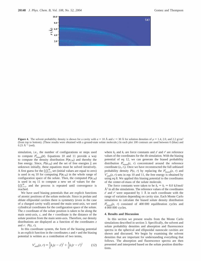
Figure 4. The solvent probability density is shown for a cavity witha ) 10 Å andc ) 30 Å for solution densities ofF ) 1.4, 2.0, and 2.2 g/cm3

(from top to bottom). (These results were obtained with a ground-state solute molecule.) In each plot 100 contours are used between 0 (blue) and0.23 Å-3 (red).

Vumbi (z, r) ) 1

2kz(z - zi)2 + 1

2kr(r - ri)2 (12)


4.1. Solvent Probability Density.4.1.1. Prolate EllipsoidalCaVities. The solvent probability density as a function of thecylindrical coordinatesz and r (see section 3.2) is shown inFigure 3 for prolate ellipsoidal cavities with semi-axisa fixedat 10 Å and the semi-axisc equal to 10, 15, 30, and 50 Å forsolutions with density equal to 2.0 g/cm3. A comparison of thesolvent probability densities in cavities witha ) 10 Å andc )30 Å and solution densities of 1.4, 2.0, and 2.2 g/cm3 is givenin Figure 4. The solvent probability densities were simulatedwith the solute molecule in the ground state. Solvent densitieswith the solute molecule in the excited state are very similar tothose shown in Figures 3 and 4. The solvent probability density,Psolv(z, r), is normalized to the number of solvent molecules sothat

whereN is the total number of molecules including the solute(see Table 2).

From Figures 3 and 4, a layered structure of the solventdensity parallel to the cavity surface can be clearly seen. Themagnitude of the density oscillations increases with the solutiondensity. For the spherical cavity (a ) c ) 10 Å), we can seethat the solvent probability density has spherical symmetry. Forthis cavity, there are two layered regions: one of high probabilitydensity near the cavity wall and the other near the center of thecavity. For the prolate ellipsoidal cavities, two layered regionsof high probability density are also observed, but in thesecavities the density peaks on the main semi-axisc in the intervalsz ) 5-7, 13.5-18, and 22.5-31 Å for cavities withc ) 15,30, and 50 Å, respectively. It can be seen from Figure 4 thatthe maximum peaks of the probability density shift toward thecavity wall as the solution density increases. The separationbetween the solvent layers is approximately 4 Å, which is similarto the Lennard-Jones diameter for the solvent molecule (see

Figure 5. The solvent probability density is shown for cavities witha ) 10, 15, and 30 Å (from left to right) andc ) 10 Å for a solution densityof F ) 2.0 g/cm3. (These results were obtained with a ground-state solute molecule.) In each plot 100 contours are used between 0 (blue) and themaximum probability density (red) of (a) 0.142 Å-3, (b) 0.062 Å-3, and (c) 0.085 Å-3.

∫0

cdz∫0

ax1-z2/c2 2πr dr Psolv(z, r) ) N - 1 (13)

Figure 6. The absorption and fluorescence spectra are plotted forprolate ellipsoidal cavities witha ) 10 Å andc ) 10 (solid lines), 15(dashed lines), 30 (dot-dashed lines), and 50 Å (dot-dot-dashed lines)for solution densities of (a) 1.4 g/cm3, (b) 2.0 g/cm3, and (c) 2.2 g/cm3

(c ) 10, 15, and 30 Å only). All of the absorption spectra and thefluorescence spectra forc g 15 Å are plotted but are difficult todistinguish due to their strong similarity; see Table 3.


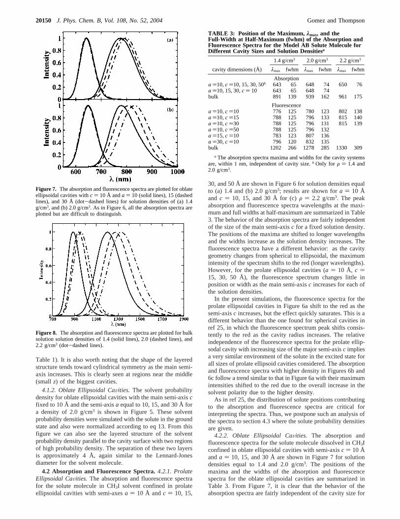
Table 1). It is also worth noting that the shape of the layeredstructure tends toward cylindrical symmetry as the main semi-axis increases. This is clearly seen at regions near the middle(small z) of the biggest cavities.

4.1.2. Oblate Ellipsoidal CaVities. The solvent probabilitydensity for oblate ellipsoidal cavities with the main semi-axiscfixed to 10 Å and the semi-axisa equal to 10, 15, and 30 Å fora density of 2.0 g/cm3 is shown in Figure 5. These solventprobability densities were simulated with the solute in the groundstate and also were normalized according to eq 13. From thisfigure we can also see the layered structure of the solventprobability density parallel to the cavity surface with two regionsof high probability density. The separation of these two layersis approximately 4 Å, again similar to the Lennard-Jonesdiameter for the solvent molecule.

4.2 Absorption and Fluorescence Spectra.4.2.1. ProlateEllipsoidal CaVities. The absorption and fluorescence spectrafor the solute molecule in CH3I solvent confined in prolateellipsoidal cavities with semi-axesa ) 10 Å andc ) 10, 15,

30, and 50 Å are shown in Figure 6 for solution densities equalto (a) 1.4 and (b) 2.0 g/cm3; results are shown fora ) 10 Åand c ) 10, 15, and 30 Å for (c)F ) 2.2 g/cm3. The peakabsorption and fluorescence spectra wavelengths at the maxi-mum and full widths at half-maximum are summarized in Table3. The behavior of the absorption spectra are fairly independentof the size of the main semi-axisc for a fixed solution density.The positions of the maxima are shifted to longer wavelengthsand the widths increase as the solution density increases. Thefluorescence spectra have a different behavior: as the cavitygeometry changes from spherical to ellipsoidal, the maximumintensity of the spectrum shifts to the red (longer wavelengths).However, for the prolate ellipsoidal cavities (a ) 10 Å, c )15, 30, 50 Å), the fluorescence spectrum changes little inposition or width as the main semi-axisc increases for each ofthe solution densities.

In the present simulations, the fluorescence spectra for theprolate ellipsoidal cavities in Figure 6a shift to the red as thesemi-axisc increases, but the effect quickly saturates. This is adifferent behavior than the one found for spherical cavities inref 25, in which the fluorescence spectrum peak shifts consis-tently to the red as the cavity radius increases. The relativeindependence of the fluorescence spectra for the prolate ellip-sodal cavity with increasing size of the major semi-axisc impliesa very similar environment of the solute in the excited state forall sizes of prolate ellipsoid cavities considered. The absorptionand fluorescence spectra with higher density in Figures 6b and6c follow a trend similar to that in Figure 6a with their maximumintensities shifted to the red due to the overall increase in thesolvent polarity due to the higher density.

As in ref 25, the distribution of solute positions contributingto the absorption and fluorescence spectra are critical forinterpreting the spectra. Thus, we postpone such an analysis ofthe spectra to section 4.3 where the solute probability densitiesare given.

4.2.2. Oblate Ellipsoidal CaVities. The absorption andfluorescence spectra for the solute molecule dissolved in CH3Iconfined in oblate ellipsoidal cavities with semi-axisc ) 10 Åanda ) 10, 15, and 30 Å are shown in Figure 7 for solutiondensities equal to 1.4 and 2.0 g/cm3. The positions of themaxima and the widths of the absorption and fluorescencespectra for the oblate ellipsoidal cavities are summarized inTable 3. From Figure 7, it is clear that the behavior of theabsorption spectra are fairly independent of the cavity size for

Figure 7. The absorption and fluorescence spectra are plotted for oblateellipsoidal cavities withc ) 10 Å anda ) 10 (solid lines), 15 (dashedlines), and 30 Å (dot-dashed lines) for solution densities of (a) 1.4g/cm3, and (b) 2.0 g/cm3. As in Figure 6, all the absorption spectra areplotted but are difficult to distinguish.

Figure 8. The absorption and fluorescence spectra are plotted for bulksolution solution densities of 1.4 (solid lines), 2.0 (dashed lines), and2.2 g/cm3 (dot-dashed lines).

TABLE 3: Position of the Maximum, λmax, and theFull-Width at Half-Maximum (fwhm) of the Absorption andFluorescence Spectra for the Model AB Solute Molecule forDifferent Cavity Sizes and Solution Densitiesa

1.4 g/cm3 2.0 g/cm3 2.2 g/cm3

cavity dimensions (Å) λmax fwhm λmax fwhm λmax fwhm

Absorptiona )10,c )10, 15, 30, 50b 643 65 648 74 650 76a )10, 15, 30,c ) 10 643 65 648 74bulk 891 139 939 162 961 175

Fluorescencea )10,c )10 776 125 780 123 802 138a )10,c )15 788 125 796 133 815 140a )10,c )30 788 125 796 131 815 139a )10,c )50 788 125 796 132a )15,c )10 783 123 807 136a )30,c )10 796 120 832 135bulk 1202 266 1278 285 1330 309

a The absorption spectra maxima and widths for the cavity systemsare, within 1 nm, independent of cavity size.b Only for F ) 1.4 and2.0 g/cm3.


each solution density. From Table 3, we can see that for a fixedsolution density the position of the maxima and the widths atthe half-maximum of the absorption spectra for the oblateellipsoidal cavities have approximately the same values as inspherical and prolate ellipsoidal cavities. The position of themaxima are shifted to longer wavelengths and the widthsincrease as the solution density increases. For the fluorescencespectra, different behavior is observed: as the semi-axisaincreases, the position of the maximum intensity of thefluorescence spectrum shifts consistently to the red (longerwavelengths). The behavior of the fluorescence spectra is similarto that found for spherical cavities in ref 25. Thus, this behaviorcould be explained with the same arguments. Due to the largedipole of the solute in the excited state, it is mostly found inthe interior of the cavity (see section 4.3) surrounded by acomplete solvation shell, and as the cavity size increases thepolarity in the environment of the solute increases. Thefluorescence spectra for solution density of 2.0 g/cm3 in Figure7b follow the same trend but with their maximum intensitiesshifted to longer wavelengths.

4.2.3. Bulk Solution.The absorption and fluorescence spectrafor the solute molecule in bulk CH3I solution (as approximatedwith periodic boundary conditions) are shown in Figure 8 fordensities of 1.4, 2.0, and 2.2 g/cm3. It is clear by comparisonwith Figures 6 and 7 that the cavities considered in this workare far from the bulk limit as evidenced by the considerablered shift of the spectra in the bulk relative to those in the cavities.This result is not surprising given the dimensions of the cavity

and the absence of long-range electrostatic interactions. Notethat both the absorption and fluorescence spectra shift to longerwavelengths as the density increases as was also observed inthe cavity systems.

4.3 Solute Probability Density.4.3.1. Prolate EllipsoidalCaVities.The probability densities of the solute center-of-massfor the solution density of 2.0 g/cm3 as a function of thecylindrical coordinatesz and r (see section 3.2) in prolateellipsoidal cavities with semi-axisa fixed to 10 Å and semi-axisc equal to 10, 15, and 30 Å are shown in Figures 9 and 10for the solute in the ground and excited states, respectively.These probability densities are normalized to unity so that theintegral of the probability density over all the elemental volumes2πr dz dr is equal to one.

For the spherical cavity (a ) 10 Å, c ) 10 Å), the probabilitydensity of the solute center-of-mass has spherical symmetry(within statistical error) around the center of the cavity for thesolute in the ground (Figure 9a) and excited (Figure 10a) states.In the ground state we can see that the solute is most likely tobe found near the cavity wall and, with a much lowerprobability, nearer the center of the spherical cavity (Figure 9a).For the prolate ellipsoidal cavities (Figures 9b and 9c), the mostprobable region is also near the cavity wall, but in these casesthere appear peaks of maximum probability at the “end” of theellipsoid along semi-axisc (here maximumz). Smaller peaksin the probabilities are also found in the interior of the cavityalong the main semi-axis aroundz ) 6 and 16.5 Å for cavitieswith c ) 15 and 30 Å, respectively.

Figure 9. The probability density of the solute center-of-mass with the solute molecule in its ground state is shown for cavities witha ) 10 Å andc ) 10, 15, and 30 Å (panels (a), (b), and (c), respectively) for a solution density ofF ) 2.0 g/cm3. In each plot 100 contours are used between0 (blue) and the maximum probability density (red) of (a) 4.56× 10-3 Å-3, (b) 3.57× 10-3 Å-3, and (c) 6.54× 10-3 Å-3.


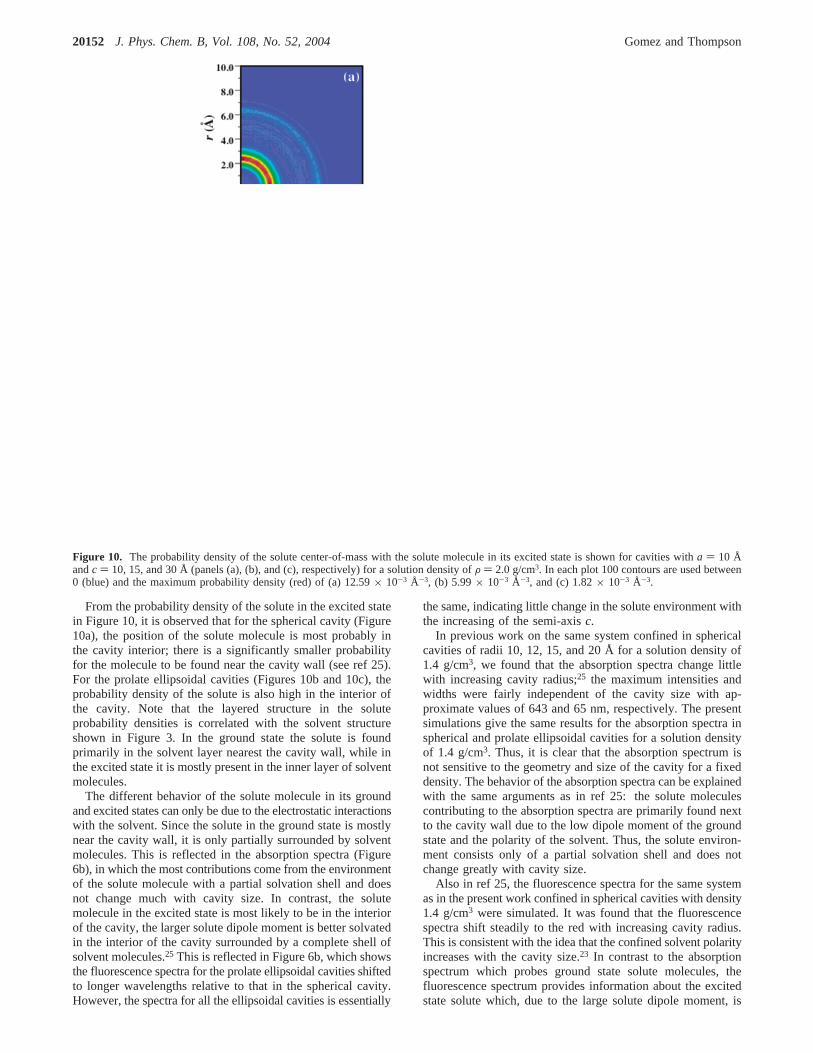
From the probability density of the solute in the excited statein Figure 10, it is observed that for the spherical cavity (Figure10a), the position of the solute molecule is most probably inthe cavity interior; there is a significantly smaller probabilityfor the molecule to be found near the cavity wall (see ref 25).For the prolate ellipsoidal cavities (Figures 10b and 10c), theprobability density of the solute is also high in the interior ofthe cavity. Note that the layered structure in the soluteprobability densities is correlated with the solvent structureshown in Figure 3. In the ground state the solute is foundprimarily in the solvent layer nearest the cavity wall, while inthe excited state it is mostly present in the inner layer of solventmolecules.

The different behavior of the solute molecule in its groundand excited states can only be due to the electrostatic interactionswith the solvent. Since the solute in the ground state is mostlynear the cavity wall, it is only partially surrounded by solventmolecules. This is reflected in the absorption spectra (Figure6b), in which the most contributions come from the environmentof the solute molecule with a partial solvation shell and doesnot change much with cavity size. In contrast, the solutemolecule in the excited state is most likely to be in the interiorof the cavity, the larger solute dipole moment is better solvatedin the interior of the cavity surrounded by a complete shell ofsolvent molecules.25 This is reflected in Figure 6b, which showsthe fluorescence spectra for the prolate ellipsoidal cavities shiftedto longer wavelengths relative to that in the spherical cavity.However, the spectra for all the ellipsoidal cavities is essentially

the same, indicating little change in the solute environment withthe increasing of the semi-axisc.

In previous work on the same system confined in sphericalcavities of radii 10, 12, 15, and 20 Å for a solution density of1.4 g/cm3, we found that the absorption spectra change littlewith increasing cavity radius;25 the maximum intensities andwidths were fairly independent of the cavity size with ap-proximate values of 643 and 65 nm, respectively. The presentsimulations give the same results for the absorption spectra inspherical and prolate ellipsoidal cavities for a solution densityof 1.4 g/cm3. Thus, it is clear that the absorption spectrum isnot sensitive to the geometry and size of the cavity for a fixeddensity. The behavior of the absorption spectra can be explainedwith the same arguments as in ref 25: the solute moleculescontributing to the absorption spectra are primarily found nextto the cavity wall due to the low dipole moment of the groundstate and the polarity of the solvent. Thus, the solute environ-ment consists only of a partial solvation shell and does notchange greatly with cavity size.

Also in ref 25, the fluorescence spectra for the same systemas in the present work confined in spherical cavities with density1.4 g/cm3 were simulated. It was found that the fluorescencespectra shift steadily to the red with increasing cavity radius.This is consistent with the idea that the confined solvent polarityincreases with the cavity size.23 In contrast to the absorptionspectrum which probes ground state solute molecules, thefluorescence spectrum provides information about the excitedstate solute which, due to the large solute dipole moment, is

Figure 10. The probability density of the solute center-of-mass with the solute molecule in its excited state is shown for cavities witha ) 10 Åandc ) 10, 15, and 30 Å (panels (a), (b), and (c), respectively) for a solution density ofF ) 2.0 g/cm3. In each plot 100 contours are used between0 (blue) and the maximum probability density (red) of (a) 12.59× 10-3 Å-3, (b) 5.99× 10-3 Å-3, and (c) 1.82× 10-3 Å-3.


found primarily in the cavity interior surrounded by a completesolvation shell. Thus, the absorption and fluorescence spectraillustrate the importance and variability of the solute position.In this model system, because of the difference in ground andexcited-state solute position distributions, the fluorescencespectrum is more sensitive to any change in solvent polarity,e.g., through increasing the cavity size, while the absorptionspectrum is essentially unchanged. However, for the prolateellipsoidal cavities considered, the environment of the excitedstate solute, which lies primarily in the cavity interior, isrelatively insensitive to the semi-axisc. Instead, in this locationthe solute fluorescence spectrum is controlled by thea semi-axis; crudely, these simulations indicate a rapid onset of thecylindrical limit.

4.3.2. Oblate Ellipsoidal CaVities. The probability densitiesof the solute center-of-mass for a solution density of 2.0 g/cm3

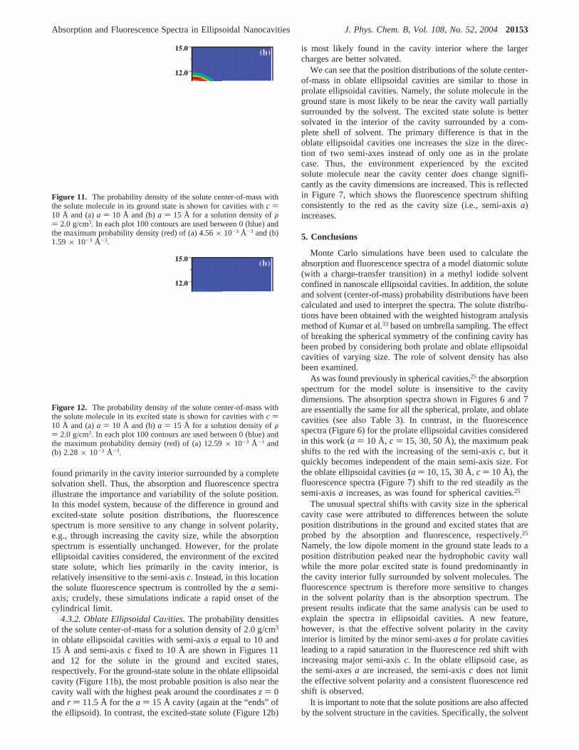
in oblate ellipsoidal cavities with semi-axisa equal to 10 and15 Å and semi-axisc fixed to 10 Å are shown in Figures 11and 12 for the solute in the ground and excited states,respectively. For the ground-state solute in the oblate ellipsoidalcavity (Figure 11b), the most probable position is also near thecavity wall with the highest peak around the coordinatesz ) 0andr ) 11.5 Å for thea ) 15 Å cavity (again at the “ends” ofthe ellipsoid). In contrast, the excited-state solute (Figure 12b)

is most likely found in the cavity interior where the largercharges are better solvated.

We can see that the position distributions of the solute center-of-mass in oblate ellipsoidal cavities are similar to those inprolate ellipsoidal cavities. Namely, the solute molecule in theground state is most likely to be near the cavity wall partiallysurrounded by the solvent. The excited state solute is bettersolvated in the interior of the cavity surrounded by a com-plete shell of solvent. The primary difference is that in theoblate ellipsoidal cavities one increases the size in the direc-tion of two semi-axes instead of only one as in the prolatecase. Thus, the environment experienced by the excitedsolute molecule near the cavity centerdoeschange signifi-cantly as the cavity dimensions are increased. This is reflectedin Figure 7, which shows the fluorescence spectrum shiftingconsistently to the red as the cavity size (i.e., semi-axisa)increases.

5. Conclusions

Monte Carlo simulations have been used to calculate theabsorption and fluorescence spectra of a model diatomic solute(with a charge-transfer transition) in a methyl iodide solventconfined in nanoscale ellipsoidal cavities. In addition, the soluteand solvent (center-of-mass) probability distributions have beencalculated and used to interpret the spectra. The solute distribu-tions have been obtained with the weighted histogram analysismethod of Kumar et al.33 based on umbrella sampling. The effectof breaking the spherical symmetry of the confining cavity hasbeen probed by considering both prolate and oblate ellipsoidalcavities of varying size. The role of solvent density has alsobeen examined.

As was found previously in spherical cavities,25 the absorptionspectrum for the model solute is insensitive to the cavitydimensions. The absorption spectra shown in Figures 6 and 7are essentially the same for all the spherical, prolate, and oblatecavities (see also Table 3). In contrast, in the fluorescencespectra (Figure 6) for the prolate ellipsoidal cavities consideredin this work (a ) 10 Å, c ) 15, 30, 50 Å), the maximum peakshifts to the red with the increasing of the semi-axisc, but itquickly becomes independent of the main semi-axis size. Forthe oblate ellipsoidal cavities (a ) 10, 15, 30 Å,c ) 10 Å), thefluorescence spectra (Figure 7) shift to the red steadily as thesemi-axisa increases, as was found for spherical cavities.25

The unusual spectral shifts with cavity size in the sphericalcavity case were attributed to differences between the soluteposition distributions in the ground and excited states that areprobed by the absorption and fluorescence, respectively.25

Namely, the low dipole moment in the ground state leads to aposition distribution peaked near the hydrophobic cavity wallwhile the more polar excited state is found predominantly inthe cavity interior fully surrounded by solvent molecules. Thefluorescence spectrum is therefore more sensitive to changesin the solvent polarity than is the absorption spectrum. Thepresent results indicate that the same analysis can be used toexplain the spectra in ellipsoidal cavities. A new feature,however, is that the effective solvent polarity in the cavityinterior is limited by the minor semi-axesa for prolate cavitiesleading to a rapid saturation in the fluorescence red shift withincreasing major semi-axisc. In the oblate ellipsoid case, asthe semi-axesa are increased, the semi-axisc does not limitthe effective solvent polarity and a consistent fluorescence redshift is observed.

It is important to note that the solute positions are also affectedby the solvent structure in the cavities. Specifically, the solvent

Figure 11. The probability density of the solute center-of-mass withthe solute molecule in its ground state is shown for cavities withc )10 Å and (a)a ) 10 Å and (b)a ) 15 Å for a solution density ofF) 2.0 g/cm3. In each plot 100 contours are used between 0 (blue) andthe maximum probability density (red) of (a) 4.56× 10-3 Å-3 and (b)1.59× 10-3 Å-3.

Figure 12. The probability density of the solute center-of-mass withthe solute molecule in its excited state is shown for cavities withc )10 Å and (a)a ) 10 Å and (b)a ) 15 Å for a solution density ofF) 2.0 g/cm3. In each plot 100 contours are used between 0 (blue) andthe maximum probability density (red) of (a) 12.59× 10-3 Å-3 and(b) 2.28× 10-3 Å-3.


packs in “layers” separated roughly by the van der Waaldiameter of the solvent molecule (here∼4 Å). The layering ofa liquid at the interface with a solid surface is a well-knownphenomenon that was observed previously in spherical cavi-ties.25,26 The local solvent density in these layers increases asthe total solution density in the cavity increases (see Figure 4).In addition, as the major semi-axisc is increased in the prolateellipsoidal cavities, the solvent density approaches cylindricalsymmetry near the cavity interior (smallz). The solvent densitynaturally affects the solute position distributions leading tolayered structures and a significant density in the solute groundstate to be found near the ellipsoid “ends” where the solventdensity is smaller.

Acknowledgment. This work was supported by the Chemi-cal Sciences, Geosciences and Biosciences Division, Office ofBasic Energy Sciences, Office of Science, U.S. Department ofEnergy.

References and Notes

(1) Brinker, C. J.; Scherer, G. W.Sol-Gel Science: The Physics andChemistry of Sol-Gel Processing; Academic Press: New York, 1990.

(2) See, e.g., Fendler, J. H.J. Phys. Chem.1980, 84, 1485-1491. Pileni,M. P., Ed.;Structure and ReactiVity in ReVerse Micelles; Elsevier: NewYork, 1989.

(3) See, e.g., Rebek, J., Jr.Acc. Chem. Res.1999, 32, 278-286.MacGillivray, L. R.; Atwood, J. L.AdV. Supramolec. Chem.2000, 6, 157-183. Steed, J. W.; Atwood, J. L.Supramolecular Chemistry; Wiley: NewYork, 2000.

(4) A recent example is Gu, L.-Q.; Cheley, S.; Bayley, H.Science2001,291, 636-640.

(5) See, e.g., De Vos, D. E.; Dams, M.; Sels, B. F.; Jacobs, P. A.Chem.ReV. 2002, 102, 3615-3640.

(6) Bhattacharyya, K.; Bagchi, B.J. Phys. Chem. A2000, 104, 10603-10613.

(7) Zhang, J.; Jonas, J.J. Phys. Chem.1993, 97, 8812-8815. Korb,J.-P.; Xu, S.; Jonas, J.J. Chem. Phys.1993, 98, 2411-2422. Korb, J.-P.;Malier, L.; Cros, F.; Xu, S.; Jonas, J.Phys. ReV. Lett. 1996, 77, 2312-2315. Korb, J.-P.; Xu, S.; Cros, F.; Malier, L.; Jonas, J.J. Chem. Phys.1997, 107, 4044-4050.

(8) Loughnane, B. J.; Fourkas, J. T.J. Phys. Chem. B1998, 102,10288-10294. Loughnane, B. J.; Scodinu, A.; Fourkas, J. T.J. Phys. Chem.B 1999, 103, 6061-6068. Loughnane, B. J.; Farrer, R. A.; Scodinu, A.;Reilly, T.; Fourkas, J. T.J. Phys. Chem. B2000, 104, 5421-5429. Farrer,R. A.; Fourkas, J. T.Acc. Chem. Res.2003, 36, 605-612.

(9) Streck, C.; Mel’nichenko, Y. B.; Richert, R.Phys. ReV. B 1996,53, 5341-5347. Richert, R.Phys. ReV. B 1996, 54, 15762-15766.

(10) Pal, S. K.; Sukul, D.; Mandal, D.; Sen, S.; Bhattacharyya, K.J.Phys. Chem. B2000, 104, 2613-2616.

(11) Wang, H.; Bardo, A. M.; Collinson, M. M.; Higgins, D. A.J.Phys. Chem. B1998, 102, 7231-7237. Mei, E.; Bardo, A. M.; Collinson,M. M.; Higgins, D. A. J. Phys. Chem. B2000, 104, 9973-9980.

(12) Baumann, R.; Ferrante, C.; Deeg, F. W.; Bra¨uchle, C.J. Chem.Phys. 2001, 114, 5781-5791. Baumann, R.; Ferrante, C.; Kneuper, E.; Deeg,F. W.; Brauchle, C.J. Phys. Chem. A2003, 107, 2422-2430.

(13) Sarkar, N.; Das, K.; Datta, A.; Das, S.; Bhattacharyya, K.J. Phys.Chem.1996, 100, 10523-10527.

(14) Riter, R. E.; Willard, D. M.; Levinger, N. E.J. Phys. Chem. B1998, 102, 2705-2714. Pant, D.; Riter, R. E.; Levinger, N. E.J. Chem.Phys.1998, 109, 9995-10003. Riter, R. E.; Undiks, E. P.; Kimmel, J. R.;Levinger, N. E.J. Phys. Chem. B1998, 102, 7931-7938. Willard, D. M.;Ritter, R. E.; Levinger, N. E.J. Am. Chem. Soc.1998, 120, 4151-4160.Willard, D. M.; Levinger, N. E.J. Phys. Chem. B2000, 104, 11075-11080.Pant, D.; Levinger, N. E.Langmuir2000, 16, 10123-10130. Riter, R. E.;Undiks, E. P.; Levinger, N. E.J. Am. Chem. Soc.1998, 120, 6062-6067.Riter, R. E.; Kimmel, J. R.; Undiks, E. P.; Levinger, N. E.J. Phys. Chem.B 1997, 101, 8292-8297.

(15) Brown, D.; Clarke, J. H. R.J. Phys. Chem.1988, 92, 2881-2888.(16) Linse, P.J. Chem. Phys.1989, 90, 4992-5004 1989. Linse, P.;

Halle, B. Mol. Phys.1989, 67, 537-573.(17) Faeder, J.; Ladanyi, B. M.J. Phys. Chem. B2000, 104, 1033-

1046.(18) Faeder, J.; Ladanyi, B. M.J. Phys. Chem. B2001, 105, 11148-

11158.(19) Das, K.; Sarkar, N.; Das, S.; Datta, A.; Bhattacharyya, K.Chem.

Phys. Lett.1996, 249, 323-328.(20) Nandi, N.; Bagchi, B.J. Phys. Chem.1996, 100, 13914-13919.(21) See, e.g., Ping, G.; Yuan, J. M.; Vallieres, M.; Dong, H.; Sun, Z.;

Wei, Y.; Li, F. Y.; Lin, S. H.J. Chem. Phys.2003, 118, 8042-8048. Friedel,M.; Sheeler, D. J.; Shea, J.-E.J. Chem. Phys.2003, 118, 8106-8113.

(22) Senapati, S.; Chandra, A.J. Chem. Phys.1999, 111, 1223-1230.(23) Senapati, S.; Chandra, A.J. Chem. Phys. B2001, 105, 5106-5109.(24) Turner, C. H.; Brennan, J. K.; Johnson, J. K.; Gubbins, K. E.J.

Chem. Phys.2002, 116, 2138-2148.(25) Thompson, W. H.J. Chem. Phys.2002, 117, 6618-6628.(26) Thompson, W. H.J. Chem. Phys.2004, 120, 8125-8133.(27) Freitas, F. F. M.; Fernandes, F. M. S. S.; Cabral, B. J. C.J. Phys.

Chem.1995, 99, 5180-5186.(28) See, e.g., McQuarrie, D. A.Statistical Mechanics; HarperCollins:

New York, 1976.(29) Press, W. H.; Flannery, B. P.; Teukolsky, S. A.; Vetterling, W. T.

Numerical Recipes; Cambridge University Press: New York, 1986.(30) Haselgrove, C. B.Math. Comput.1961, 15, 323-337.(31) Allen, M. P.; Tildesley, D. J.Computer Simulation of Liquids;

Oxford University Press: New York, 1987.(32) Frenkel, D.; Smit, B.Understanding Molecular Simulation, from

Algorithms to Applications; Academic Press: New York, 1996.(33) Kumar, S.; Bouzida, D.; Swendsen, R. H.; Kollman, P. A.;

Rosenberg, J. M.J. Comput. Chem.1992, 13, 1011-1021. Kumar, S.;Bouzida, D.; Swendsen, R. H.; Kollman, P. A.; Rosenberg, J. M.J. Comput.Chem.1995, 16, 1339-1350.

(34) Torrie, G. M.; Valleau, J. P.J. Comput. Phys.1977, 23, 187-199.


monte carlo simulations of absorption and fluorescence spectra in ellipsoidal nanocavities

Documents