1

Master of Science Thesis in

Medical Radiation Physics

Monte Carlo Simulations of

a Clinical PET system using

the GATE Software

Henrik Bertilsson

Department of Medical Radiation Physics

Lund University, Sweden 2010

Supervisors: Michael Ljungberg

Sven-Erik Strand

Lena Jönsson

2

Abstract

Introduction: Monte Carlo simulation is a powerful tool in research in the field of nuclear

medicine imaging and there is a wide area of applications. The purpose of this work was (1)

to understand the basics of the Monte Carlo simulation software Geant4 Application for

Tomographic Emission (GATE); (2) to create a model of Philips Gemini TF PET/CT system;

(3) to run a number of simulations to compare the performance of the model to published data

for this system; and (4) to further investigate how scattered radiation affects the image quality.

Material and Methods: The software used in this work was the GATE version 4.0. A model

of Philips Gemini TF PET/CT system was defined. A program written in Fortran language

was used for data processing and image reconstruction was done in a program written in

Interactive Data Language (IDL). Simulations of spatial resolution were performed in

agreement with NEMA NU-2 specifications and full width at half maximum (FWHM) and

full width at tenth maximum (FWTM) were reported. Investigations of how scattered

radiation and random events depend on different parameters (for example phantom size,

source position and source activity) were done. Sensitivity was measured in accordance with

the NEMA NU-2 protocol, and a comparison among three different crystal materials

(Lutetium Yttrium Orthosilicate (LYSO), Bismuth Germanate (BGO) and Thallium activated

Sodium Iodine (NaI(Tl))) was done. The last step was to simulate a voxelized phantom of a

human brain and to obtain images that were reconstructed from total, true, scattered and

random events.

Results: The transverse spatial resolution was measured to be FWHM/FWTM = 5.0/8.1,

5.4/9.4 and 5.7/8.8 mm for source positions/image directions 1 cm/tangential, 10

cm/tangential and 10 cm/radial. The scatter study shows a linear dependence between scatter

fraction and phantom diameter. The random fraction shows also linear dependence on source

activity and the random rate shows a clearly quadratic dependence which is expected. The

sensitivities for the different materials were 2.6, 9.1 and 1.1 cps/kBq for LYSO, BGO and

NaI(Tl), respectively. The result for LYSO does not agree with published data, a deviation

likely due to the fact that the material defined in the GATE material database does not have

the same density as the real material. Images from the voxelized brain phantom simulation

agree with the phantom image but no major difference was seen between images

reconstructed from total events compared to those reconstructed from true events.

Conclusion: GATE is a powerful tool in research in nuclear medicine imaging. It is easy to

define and simulate complex situations but the long simulation time and difficulties in data

post processing are this software’s main drawbacks. However its advantages compared to

other existing Monte Carlo simulation software for emission tomography makes this software

to an important tool that will play a major role in future research within this field.

3

Henrik Bertilsson

Kan beräkningar ge mer information om verkligheten än

verkligheten själv?

Monte Carlo-simuleringar har fått en ökad betydelse som forskningsverktyg inom

nuklearmedicinsk bildgivning eftersom man på ett mycket kontrollerat sätt kan studera

nästan vad man vill. I denna studie har datorsimuleringar av ett PET-system gjorts med

ett program som heter GATE.

PET (Positron Emission Tomography) är en nuklearmedicinsk bildgivningsteknik som

används mer och mer inom sjukvården som ett viktigt hjälpmedel för att upptäcka cancer.

Tekniken bygger på att man injicerar ett radioaktivt läkemedel i kroppen som med dess

kemiska egenskaper tas upp i önskvärd vävnad, t.ex. cancertumörer. Det radioaktiva

sönderfallet resulterar i fotonstrålning som i sin tur kan detekteras av PET-systemet för att

sedan ge digitala bilder som visar omsättningen av läkemedlet i olika delar av kroppen.

Monte Carlo-tekniken bygger på att man i ett datorprogram efterliknar ett bildsystem (t.ex. ett

PET-system) och med hjälp av sannolikhetsteorier och slumptal försöker att förutse vad som

skulle ha skett i verkligheten. Namnet har sitt ursprung från kasinospel i Monaco, ett ställe där

slump och sannolikhet har stor betydelse. Genom att känna till sannolikheter för hur t.ex.

fotonstrålning sprids i olika material, så kan man med hjälp av kraftfulla datorer beräkna hur

massor av fotoner skulle ha betett sig i verkligheten. Denna teknik lämpar sig därför väl för

PET där miljontals fotoner produceras varje sekund.

I detta arbete har en modell av ett PET-system, som används dagligen på sjukhuset, byggts

med hjälp av ett Monte Carlo-program som heter GATE och är anpassat för just

nuklearmedicinsk bildgivning. I arbetet simulerades PET-systemets prestanda vilka sedan

jämfördes med experimentella mätningar och publicerade data av det verkliga systemet.

Dessutom studerades i vilken omfattning spridd strålning försämrar kvaliteten hos de slutliga

bilderna. Här visar studien på den verkliga styrkan med Monte Carlo-simuleringar d.v.s.

möjligheten att få ut information som är omöjlig vid experimentella mätningar.

Handledare: Michael Ljungberg Examensarbete 30 hp i Medicinsk strålningsfysik* 2010 Avd för Medicinsk strålningsfysik, IKVL, Lunds universitet

*Examensarbetsämne: se kursplan

4

Abbreviations

2D Two-dimensional

3D Three-dimensional

3DRAMLA 3D row-action maximum-likelihood algorithm

3DRP 3D reprojection method

BGO Bismuth Germanate

CT Computed tomography

ECT Emission computed tomography

FBP Filtered backprojection

FDG Fluorodeoxyglucose

FORE Fourier rebinning

FOV Field of view

FWHM Full width at half maximum

FWTM Full width at tenth maximum

GATE Geant4 Application for Tomographic Emission

IDL Interactive Data Language

LOR Line of response

LSO Lutetium Oxyorthosilicate

LYSO Lutetium Yttrium Orthosilicate

ML-EM Maximum-likelihood expectation-maximization

NaI(Tl) Thallium activated Sodium Iodine

OS-EM Ordered-subset expectation-maximization

PDF Probability density function

PET Positron emission tomography

PHG Photon History Generator

SimSET Simulation System for Emission Tomography

SPECT Single photon emission computed tomography

STIR Software for Tomographic Image Reconstruction

5

Table of Contents

Abstract ................................................................................................................................................... 2

Summary written in Swedish .................................................................................................................. 3

Abbreviations .......................................................................................................................................... 4

Table of Contents .................................................................................................................................... 5

1 Introduction .......................................................................................................................................... 7

1.1 Aim ................................................................................................................................................ 7

2 Background .......................................................................................................................................... 8

2.1 Positron emission tomography ...................................................................................................... 8

2.1.1 Radionuclides in PET ............................................................................................................. 8

2.1.2 PET system design ................................................................................................................. 8

2.1.3 Image quality limitations ........................................................................................................ 9

2.1.4 Data processing and image reconstruction ........................................................................... 10

2.2 Monte Carlo Simulations ............................................................................................................. 10

2.3 GATE .......................................................................................................................................... 11

2.3.1 Simulation architecture ......................................................................................................... 12

2.3.2 Imaging systems ................................................................................................................... 12

2.3.3 Source and physics ............................................................................................................... 13

2.3.4 The digitizer module............................................................................................................. 13

2.3.5 Output formats ...................................................................................................................... 13

2.4 SimSET ....................................................................................................................................... 14

3 Material and Methods ......................................................................................................................... 14

3.1 Philips Gemini TF PET/CT Scanner ........................................................................................... 14

3.2 Example of defining a PET camera in GATE ............................................................................. 15

3.3 Data Processing ........................................................................................................................... 18

3.4 Image Reconstruction .................................................................................................................. 21

3.5 Simulations .................................................................................................................................. 21

3.5.1 Spatial Resolution ................................................................................................................. 22

6

3.5.2 Scatter and Randoms ............................................................................................................ 23

3.5.3 Sensitivity ............................................................................................................................. 23

3.5.4 Brain phantom ...................................................................................................................... 24

4 Results ................................................................................................................................................ 25

4.1 Spatial resolution ......................................................................................................................... 25

4.2 Scatter and Randoms ................................................................................................................... 26

4.3 Sensitivity .................................................................................................................................... 30

4.4 Brain phantom ............................................................................................................................. 31

5 Discussion .......................................................................................................................................... 33

5.1 Spatial resolution ......................................................................................................................... 33

5.2 Scatter and Randoms ................................................................................................................... 34

5.3 Sensitivity .................................................................................................................................... 35

5.4 Brain phantom ............................................................................................................................. 36

6 Future challenges ................................................................................................................................ 36

Acknowledgments ................................................................................................................................. 37

References ............................................................................................................................................. 38

Appendix A: Sinogram program ........................................................................................................... 40

Appendix B: Reconstruction IDL-code ................................................................................................. 44

7

1 Introduction

During recent years, the importance of Monte Carlo simulations has grown in several areas of

medical physics. Emission computed tomography (ECT) is a nuclear medicine imaging

application where Monte Carlo simulations have proven to be a useful tool to study imaging

characteristics and parameters that cannot be measured experimentally. Examples of such

parameters are the contribution of scattered radiation and random counts to reconstructed

images. Single photon emission computed tomography (SPECT) and positron emission

tomography (PET) are two branches of ECT. Monte Carlo simulations can also be used in

nuclear medicine for internal dosimetry, quality controls, image registration, activity

quantification and correction of partial volume effects [1-3].

There are various public domain software packages available for Monte Carlo simulations of

parameters in ECT, but all suffer from different drawbacks (handling of complex models,

computing time etc.) The Geant4 Application for Tomographic Emission (GATE) simulation

package uses well-validated physical models and can handle complex imaging geometries [4].

A wide community of developers and users, documentation and support is connected to the

GATE software. GATE is also flexible in the setup of different system designs. However this

flexibility makes the simulations very time consuming.

To assess the accuracy of GATE Monte Carlo simulated data, it is essential to validate

simulated data against measured experimental results from commercial systems. In a

published study by Lamare et al [5], a comparison between simulated and measured data was

done for the Philips Allegro PET system. The focus of this work is another system for clinical

PET imaging, the Philips Gemini TF PET/CT system with time-of-flight capabilities.

1.1 Aim

The main aims of this project were to understand the basics of the GATE Monte Carlo

simulation package by setting up a model of the clinical Philips Gemini TF PET/CT system in

GATE, to validate the model from simulations, and to compare results from these simulations

to published performance data. In addition, the aim was to simulate the scattered radiation and

study quantitatively and qualitatively how different parameters (for example phantom size,

source activity and source location in the phantom) affect the image quality based on

simulations of a point source in cylindrical Plexiglas phantom. Also a simulation of a

voxelized phantom of a human brain was performed in order to examine how the radiation

scatter affects the image quality (that is spatial resolution and noise level).

8

2 Background

2.1 Positron emission tomography

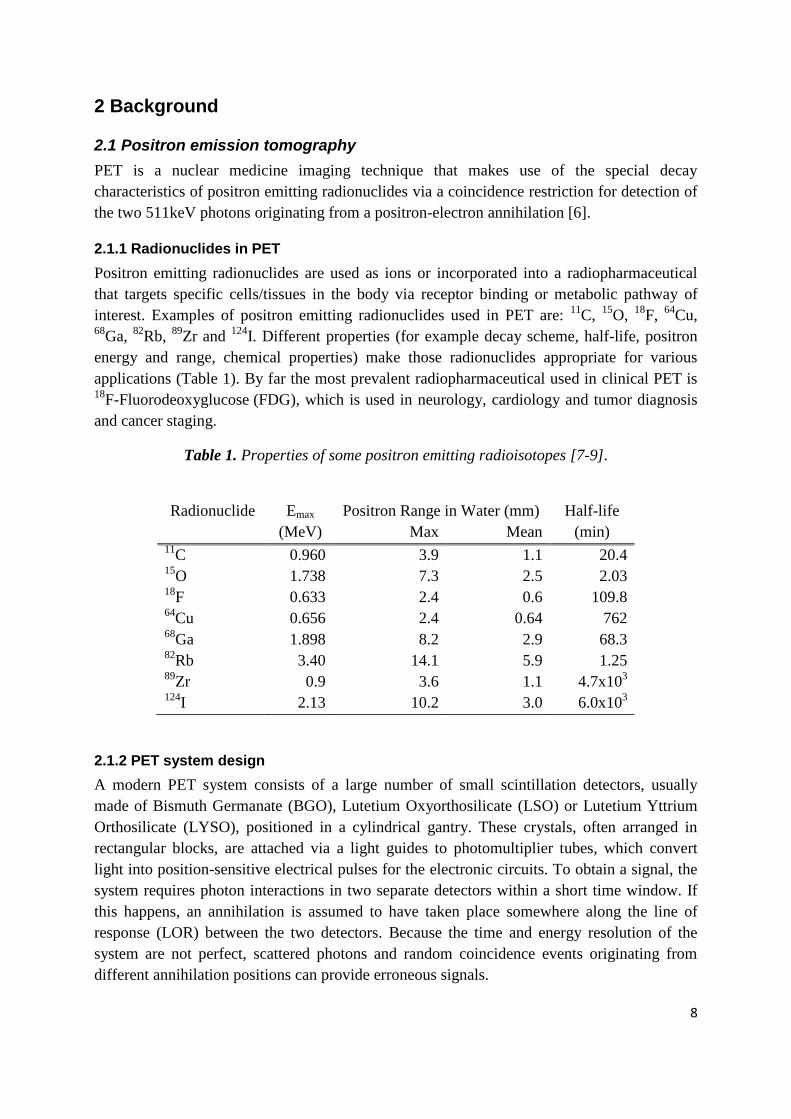
PET is a nuclear medicine imaging technique that makes use of the special decay

characteristics of positron emitting radionuclides via a coincidence restriction for detection of

the two 511keV photons originating from a positron-electron annihilation [6].

2.1.1 Radionuclides in PET

Positron emitting radionuclides are used as ions or incorporated into a radiopharmaceutical

that targets specific cells/tissues in the body via receptor binding or metabolic pathway of

interest. Examples of positron emitting radionuclides used in PET are: 11

C, 15

O, 18

F, 64

Cu, 68

Ga, 82

Rb, 89

Zr and 124

I. Different properties (for example decay scheme, half-life, positron

energy and range, chemical properties) make those radionuclides appropriate for various

applications (Table 1). By far the most prevalent radiopharmaceutical used in clinical PET is 18

F-Fluorodeoxyglucose (FDG), which is used in neurology, cardiology and tumor diagnosis

and cancer staging.

Table 1. Properties of some positron emitting radioisotopes [7-9].

Radionuclide Emax Positron Range in Water (mm) Half-life

(MeV) Max Mean (min) 11

C

0.960 3.9 1.1 20.4 15

O 1.738 7.3 2.5 2.03 18

F 0.633 2.4 0.6 109.8 64

Cu 0.656 2.4 0.64 762 68

Ga 1.898 8.2 2.9 68.3 82

Rb 3.40 14.1 5.9 1.25 89

Zr 0.9 3.6 1.1 4.7x103

124I 2.13 10.2 3.0 6.0x10

3

2.1.2 PET system design

A modern PET system consists of a large number of small scintillation detectors, usually

made of Bismuth Germanate (BGO), Lutetium Oxyorthosilicate (LSO) or Lutetium Yttrium

Orthosilicate (LYSO), positioned in a cylindrical gantry. These crystals, often arranged in

rectangular blocks, are attached via a light guides to photomultiplier tubes, which convert

light into position-sensitive electrical pulses for the electronic circuits. To obtain a signal, the

system requires photon interactions in two separate detectors within a short time window. If

this happens, an annihilation is assumed to have taken place somewhere along the line of

response (LOR) between the two detectors. Because the time and energy resolution of the

system are not perfect, scattered photons and random coincidence events originating from

different annihilation positions can provide erroneous signals.

9

2.1.3 Image quality limitations

There are at least three factors that ultimately affect spatial resolution in PET. The first comes

from the fact that the emitted positrons have a non-zero range before the annihilation. The

main interest for a PET study is to determine the tissue distribution of the

radiopharmaceutical. However a PET image shows the annihilation sites. If the positron range

is large then, this will introduce an uncertainty in the interpretation of the image. The

positron range depends mainly on the energy of the emitted particle (for example 18

F has a

mean positron range in water of 0.6 mm compared to 82

Rb with 5.9 mm) and the density of

the material in which the radiodecay occurs. The second factor comes from the fact that not

all of the positrons are at rest when the annihilation occurs. This causes non-colinearity which

means that the two 511 keV photons emitted will not be emitted exactly 180° apart because of

the momentum conservation [6]. The average angular deviation is about 0.25° from 180°

which causes a small error in event positioning (maximum 1 mm for 0.25° in a 90 cm

diameter gantry). A third factor that reduces the spatial resolution is the non-zero size of the

crystals. Each crystal in a human PET system typically has a size of about 4 mm in the

projection plane which makes this factor highly significant.

There are also some limitations in the coincidence detection technique that cause image

degradation in PET imaging. Four types of coincidence events exist:

1. True events are those where the two detected photons come from the same

annihilation without having undergone any interaction in the object from the point of

annihilation to the crystals (Figure 1 a).

2. Scattered events occur when one or both of the detected photons have interacted with

surrounding tissue and therefore changed direction resulting in mispositioning of the

event (Figure 1 b).

3. Random coincidence is when two photons from different annihilation processes are

detected within the coincidence window (Figure 1 c).

4. Multiple coincidences occur when three or more photons are detected simultaneously

within the coincidence window (Figure 1 d).

Figure 1. Illustration of the four different kinds of coincidences that can occur. a) true events

b) scattered events c) random events and d) multiple events. The blue lines illustrate the

LORs.

a b c d

10

A system with perfect energy resolution would eliminate scattered events, and improved

timing resolution would reduce effects from random and multiple events [6].

The PET system of today acquires data in three-dimensional (3D) mode, which means that

coincidences in all crystal combinations within the field of view (FOV) get registered as

events. The older PET systems acquired data in two-dimensional (2D) mode, where detector

rings were separated by tungsten septa and a signal could only occur from coincidences in a

very limited number of adjacent parallel planes.

2.1.4 Data processing and image reconstruction

A sinogram is a matrix in which the acquired data are sorted in a certain way that makes it

possible to reconstruct tomographic images. Each row in this matrix contains data for Lines of

response (LOR) at a particular angle, and each column corresponds to a different radial offset

from the scanner center. Every element in the sinogram matrix corresponds to a pair of

detectors that can generate a coincidence signal. In a 2D acquisition mode, the data are sorted

into parallel sinograms and then reconstructed using a 2D reconstruction algorithm. In 3D

acquisition, the data are stored into sets of oblique sinograms, and thereafter either i)

reconstructed directly using a 3D algorithm or ii) the sinograms are rebinned to form a set of

2D sinograms using either a single-slice rebinning algorithm where coincidences from

different adjacent detector rings are placed in the sinogram slice corresponding to the center

location of the contributing rings [10, 11], or the more sophisticated Fourier Rebinning

(FORE) algorithm [12]. The latter technique makes it possible to use the faster 2D

reconstruction algorithms described below.

After the data are sorted either into 2D sinograms, or into a 3D data stack, images can be

reconstructed using a suitable algorithm. The most common 2D tomographic reconstruction

algorithm has been filtered backprojection (FBP), which is a fast analytical method. There are

also iterative tomographic reconstruction algorithms available such as the maximum-

likelihood expectation-maximization (ML-EM) [13], and the accelerated ordered-subset

expectation-maximization (OS-EM) [14] method, both having the advantage of better noise

characteristics than the FBP method, as well as the possibility to handle various corrections,

such as non-homogeneous attenuation and scatter correction, within the reconstruction

process itself. The main disadvantage of iterative reconstruction is the relatively long time it

takes to perform the reconstruction. Data collected in 3D can be reconstructed using 3D

reprojection (3DRP) [15] or 3D row-action maximum-likelihood algorithm (3D RAMLA)

[16]. Iterative 3D reconstruction algorithms are also possible to use, but these are even more

time consuming. Comparisons among different reconstruction algorithms can be done using

data received from Monte Carlo simulations.

2.2 Monte Carlo Simulations

The Monte Carlo method can be used to simulate many complex processes and phenomena by

statistical methods using random numbers. In a Monte Carlo analysis of PET, a computer

model is created with characteristics as similar as possible to the real imaging system. In this

model the photon and charged particle interactions are simulated based on known

11

probabilities of occurrence, with sampling of the probability density functions (PDFs) using

uniformly distributed random numbers. The simulation is similar to a real measurement in

that the statistical uncertainty decreases as the number of events increases, and therefore the

quality of the reported average behavior improves [17-19].

To evaluate the trajectories and energies deposited at different locations in medical imaging,

for example ECT, the radiation transport is simulated by sampling the PDFs for the

interactions of the charged particles or photons.

Monte Carlo simulation is an excellent method for studying differences in image quality when

using radionuclides with various positron ranges [20]. Using Monte Carlo simulation it is also

possible to study parameters that are not possible to measure directly, for example the

behavior of scattered photons [21]. It is also a good method to use when developing and

evaluating new correction algorithms, and also when comparing different PET detector

materials in order to improve performance [22]. One way to optimize the detector

configuration and design of a PET system and to improve the outcome of examinations is to

use Monte Carlo simulations, because it is easy to change one parameter at a time in the

model [23]. Monte Carlo implementations have been used for scatter correction in iterative

reconstruction algorithms [24, 25].

Two major categories of Monte Carlo simulator software exist.

1. General purpose software such as EGS4 [26], ITS [27], MCNP [28] and Geant4 [29].

These programs have mainly been developed for high energy physics and include a

complete set of particle and cross-section data up to several GeV.

2. Monte Carlo simulation programs dedicated to SPECT and PET. Examples are

SimSET [30], SIMIND [31], PETSIM [32], PET-SORTEGO [33] and GATE [4].

These programs have been designed to solve problems for a specific type of imaging

system and can be very fast because of large optimization including the use of

variance reduction methods. The major drawback may be limited flexibility when

simulating different types of geometries.

2.3 GATE

In 2001, a workshop was organized in Paris about the future of Monte Carlo simulations in

nuclear medicine. From the discussions about drawbacks with available software, it became

clear that a new dedicated toolkit for tomographic emission was needed which could handle

decay kinetics, dead time and movements. An object-oriented solution was preferred. The

coding began with the Lausanne PET instrumentation group with help from several other

physics and signal processing groups. A workshop was organized the year after to define the

development strategy. In 2002, the first OpenGATE meeting took place in Lausanne, with the

first live demonstration of the first version of GATE. Since then a number of new versions has

been released [34].

The simulation software used in this study was the GATE [4] software version 4.0. This

program is dedicated to simulation of PET and SPECT systems. It is based on the Geant4

12

Monte Carlo code [29] and uses Geant4’s libraries to simulate particle transport. The basic

idea with GATE is that the user should not need to carry out any C++ programming, but

instead employ an extended version of Geant4 script language. The program has a layered

architecture with a core layer that defines the main tools and features of GATE in C++, an

application layer with C++ base classes and at the top, a user layer where the simulations are

set up using command based scripts.

One feature of GATE is the possibility of simulating time-dependent phenomena such as

source kinetics and movements of geometries, for example patient motion, respiratory and

cardiac motion, changes of activity distribution over time and scanner rotation. Geant4 does

however require static geometries during a simulation. Because of the relatively short duration

of a single event compared to a typical movement, this problem can be solved by dividing the

simulation into short time steps and updating the geometries at every step.

2.3.1 Simulation architecture

A typical GATE simulation is divided in seven steps:

1. The verbosity level is set for each simulation module. This means that it is possible to

decide the amount of information about the simulation returned by the program. In the

first step, the visualization options are also chosen.

2. The geometries are defined. In this step, the geometry, denoted “world”, in which the

simulation is going to take place is initially defined. After that the scanner and

phantom geometries are defined.

3. This step defines the detection parameters in the so called digitizer module. Here the

characteristics of the system are prescribed such as energy and timing resolution. It is

also possible to include dead time and other features related to the creation of the

image.

4. The physical processes are chosen for the simulation. This includes the choice of

interactions library, enabling or disabling interaction effects and setting cut-off energy

or range for secondary particle production.

5. The radioactive source is defined. This includes particle type, activity and half-life,

source geometry, emission angle and source movement.

6. Output format is chosen. Different output formats are available for different imaging

systems.

7. The experiment is initialized and started [35].

2.3.2 Imaging systems

A number of different imaging systems are available in GATE: (for example “scanner”,

“SPECThead”, “cylindricalPET”, “ecat”, “CPET” and “OPET”). A system is defined

as a family of geometries compatible with different data output formats. For cylindrical PET

the available output formats are: ASCII, ROOT, RAW and LMF (a specific format dedicated to

this system). Other systems have different options. The purpose of system definition is to

make the particle-in-detector interaction histories be processed realistically.

13

2.3.3 Source and physics

The radioactive source in a GATE simulation is defined by the radionuclide, particle type and

position, direction of emitted radiation, energy and activity. The radioactive decay is

performed by the Geant4 Radioactive Decay Module.

There are two packages available to simulate electromagnetic processes: the standard energy

package and the low energy package. The low energy package models photon and electron

interaction down to 250 eV and includes Rayleigh scatter and provides more accurate models

for medical application. To speed up the simulation, it is possible to set a threshold for the

production of secondary particle production [36].

2.3.4 The digitizer module

The digitizer chain simulates the electronics response of a sensitive detector, which are used

to store information about particle interaction within a volume. The digitizer chain consists of

some processing modules: the “hit adder“ that calculates the energy deposited in a

sensitive detector by a given photon, the “pulse reader“ that adds pulses from a group of

sensitive detectors yielding a pulse containing the total energy deposited in these detectors

and assigned to the position of the largest pulse. There are also some modules wherein the

user can define parameters such as energy resolution (that is the ability to sort photons of

different energies), energy window (that is the energy span within which the photons will be

registered), spatial resolution, time resolution (that is the ability to separate two events with

regard to time), dead time and coincidence window (that is the time interval within which two

detected photons will cause an event).

2.3.5 Output formats

Different output formats are available for different systems. The ASCII format, which is the

choice in this work, is the simplest. It gives all information about the detected photons in a

large text file. Each row corresponds to one event and includes information about event

number, time of annihilation, positions of annihilation, scatter, energy deposition, detecting

crystal IDs and position where detected. This output needs to be further processed to be

useful, but GATE can automatically sort out coincidence events from single photon events.

The ROOT format is also a very powerful output that can be analyzed by using special

software. With this output it is easy to get histograms over distributions of the angles between

the two annihilation photons, the energies of the positrons, the time stamps of the decays and

the ranges of the positrons. For an “ecat” system a sinogram output is available. This output

automatically stores the events in 2D sinograms. The list mode format LMF, a special output

for a “cylindricalPET” system, can be used with other software for image

reconstruction. However, only singles can be stored by GATE, which means that coincidence

events have to be paired together afterwards. The Raw output gives access to raw images of

source position for singles or coincidences. This output should be used in addition to other

formats.

14

2.4 SimSET

Simulation System for Emission Tomography (SimSET) is another well-known Monte Carlo

simulation software designed for simulations of SPECT and PET system. Although SimSET

was not used in this work, a brief description is given here as a comparison to GATE.

SimSET consists of different modules. The Photon History Generator (PHG) tracks the

photons through the tomograph FOV and creates a photon history list with information about

the photons reaching the camera. An object editor is used for definition of the activity and

attenuation objects for the PHG. The collimator routine in SimSET is based on the two-

dimensional PET collimator that originally was implemented in the Monte Carlo program

PETSIM [32]. The detector and binning modules are used to define Gaussian blurring of

energy, and the photon events are then binned by combinations of number of scatters, axial

position, angles and photon energy. The data are binned during the simulation run, but the

data can be reprocessed afterwards by the use of the photon history list. The main advantages

of GATE compared to SimSET are that GATE in contrast to SimSET can handle system dead

time, random events, block detector geometries with distances between each crystal (SimSET

can only handle continuous detector rings) and dynamic studies with time dependent

processes [4, 30, 37].

3 Material and Methods

3.1 Philips Gemini TF PET/CT Scanner

The scanner modeled in this work was the Gemini TF PET/CT (Philips Medical Systems,

Cleveland, OH). This scanner collects data in septa-less 3D mode and has time of flight

capability. The images are reconstructed using 3D RAMLA. Scanner specifications are given

in Table 2.

Table 2. Scanner specifications used

in the model for the simulations [38,

39].

Parameter Value

Energy resolution 12%

Coincidence window 3.8ns

Energy window 440-665 keV

Field of view 57.6 cm

The detector crystals are made of LYSO, and have a size of 4x4x22 mm3 each. The crystals

are organized in 28 sectors of 23x44 crystals placed in 4.0946x4.0750 mm2 arrays. The

reflector material between the crystals is of unknown chemical composition, and is in this

work assumed equivalent to Plexiglas. The crystal sectors are placed in a cylindrical gantry

15

with an inner diameter of 90.34 cm. The light-guide consists of a 14 mm thick layer of Lucite

(polyethylene). At each end of the detector array, there are two 2.5 cm thick lead shields with

a 72 cm bore opening [38-40].

The dead time characteristics of the system are unknown and dead time is therefore not taken

into account in the simulations. The simulations were run for low activities to minimize dead

time effects.

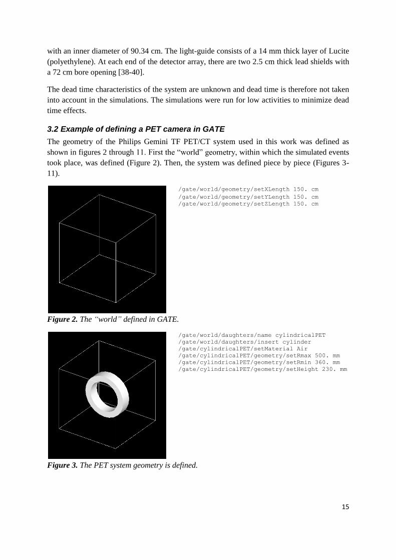
3.2 Example of defining a PET camera in GATE

The geometry of the Philips Gemini TF PET/CT system used in this work was defined as

shown in figures 2 through 11. First the “world” geometry, within which the simulated events

took place, was defined (Figure 2). Then, the system was defined piece by piece (Figures 3-

11).

/gate/world/geometry/setXLength 150. cm

/gate/world/geometry/setYLength 150. cm

/gate/world/geometry/setZLength 150. cm

Figure 2. The “world” defined in GATE.

/gate/world/daughters/name cylindricalPET

/gate/world/daughters/insert cylinder

/gate/cylindricalPET/setMaterial Air

/gate/cylindricalPET/geometry/setRmax 500. mm

/gate/cylindricalPET/geometry/setRmin 360. mm

/gate/cylindricalPET/geometry/setHeight 230. mm

Figure 3. The PET system geometry is defined.

16

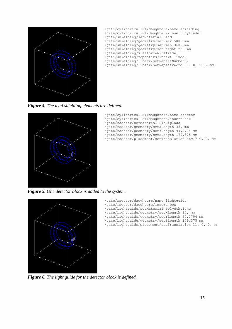
/gate/cylindricalPET/daughters/name shielding

/gate/cylindricalPET/daughters/insert cylinder

/gate/shielding/setMaterial Lead

/gate/shielding/geometry/setRmax 500. mm

/gate/shielding/geometry/setRmin 360. mm

/gate/shielding/geometry/setHeight 25. mm

/gate/shielding/vis/forceWireframe

/gate/shielding/repeaters/insert linear

/gate/shielding/linear/setRepeatNumber 2

/gate/shielding/linear/setRepeatVector 0. 0. 205. mm

Figure 4. The lead shielding elements are defined.

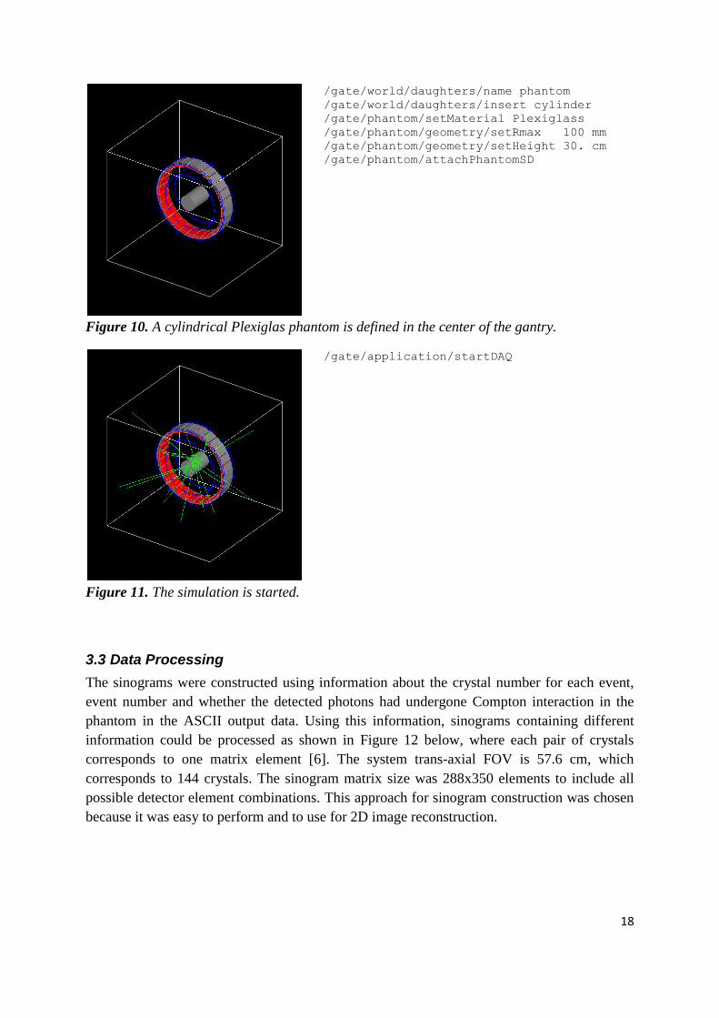
/gate/cylindricalPET/daughters/name rsector

/gate/cylindricalPET/daughters/insert box

/gate/rsector/setMaterial Plexiglass

/gate/rsector/geometry/setXLength 36. mm

/gate/rsector/geometry/setYLength 94.2704 mm

/gate/rsector/geometry/setZLength 179.375 mm

/gate/rsector/placement/setTranslation 469.7 0. 0. mm

Figure 5. One detector block is added to the system.

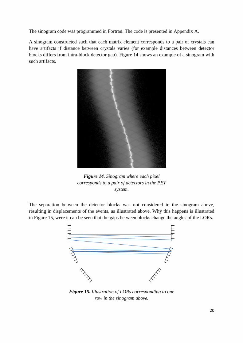
/gate/rsector/daughters/name lightguide

/gate/rsector/daughters/insert box

/gate/lightguide/setMaterial Polyethylene

/gate/lightguide/geometry/setXLength 14. mm

/gate/lightguide/geometry/setYLength 94.2704 mm

/gate/lightguide/geometry/setZLength 179.375 mm

/gate/lightguide/placement/setTranslation 11. 0. 0. mm

Figure 6. The light guide for the detector block is defined.

17

/gate/rsector/daughters/name crystal

/gate/rsector/daughters/insert box

/gate/crystal/setMaterial LYSO

/gate/crystal/geometry/setXLength 22. mm

/gate/crystal/geometry/setYLength 4. mm

/gate/crystal/geometry/setZLength 4. mm

/gate/crystal/placement/setTranslation -0.7 0. 0. mm

/gate/crystal/vis/forceSolid

/gate/crystal/vis/setColor red

Figure 7. One crystal is inserted into this detector block.

/gate/crystal/repeaters/insert cubicArray

/gate/crystal/cubicArray/setRepeatNumberX 1

/gate/crystal/cubicArray/setRepeatNumberY 23

/gate/crystal/cubicArray/setRepeatNumberZ 44

/gate/crystal/cubicArray/setRepeatVector 0. 4.0946

4.075 mm

Figure 8. Crystal insertion is repeated within one detector block so that this “rsector” is

completed.

/gate/rsector/repeaters/insert ring

/gate/rsector/ring/setRepeatNumber 28

Figure 9. Detector block creation is repeated within the gantry so that the scanner geometry

is finished.

18

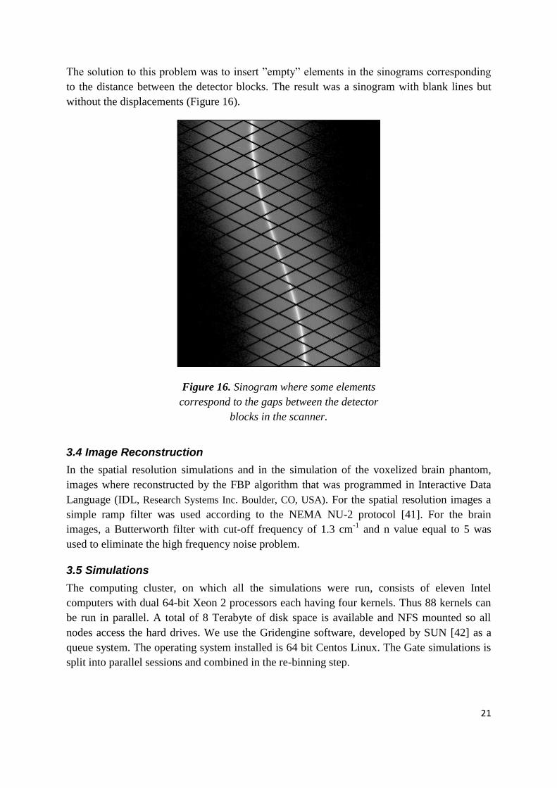
/gate/world/daughters/name phantom

/gate/world/daughters/insert cylinder

/gate/phantom/setMaterial Plexiglass

/gate/phantom/geometry/setRmax 100 mm

/gate/phantom/geometry/setHeight 30. cm

/gate/phantom/attachPhantomSD

Figure 10. A cylindrical Plexiglas phantom is defined in the center of the gantry.

/gate/application/startDAQ

Figure 11. The simulation is started.

3.3 Data Processing

The sinograms were constructed using information about the crystal number for each event,

event number and whether the detected photons had undergone Compton interaction in the

phantom in the ASCII output data. Using this information, sinograms containing different

information could be processed as shown in Figure 12 below, where each pair of crystals

corresponds to one matrix element [6]. The system trans-axial FOV is 57.6 cm, which

corresponds to 144 crystals. The sinogram matrix size was 288x350 elements to include all

possible detector element combinations. This approach for sinogram construction was chosen

because it was easy to perform and to use for 2D image reconstruction.

19

103 596

103 595

104 595

104 594

… … 245 454

245 453

246 453

246 452

104 597

104 596

105 596

105 595

… … 246 455

246 454

247 454

247 453

105 598

105 597

106 597

106 596

… … 247 456

247 455

248 455

248 454

106 599

106 598

107 598

107 597

…

…

248 457

248 456

249 456

249 455

.

. . .

.

. . .

… .

… .

.

. . .

.

. . .

.

. . .

.

. . .

… .

… .

.

. . .

.

. . .

.

. . .

.

. . .

… .

… .

.

. . .

.

. . .

449 242

449 241

450 241

450 240

… … 591 100

591 99

592 99

592 98

450 243

450 242

451 242

451 241

… … 592 101

592 100

593 100

593 99

451 244

451 243

452 243

452 242

… … 593 102

593 101

594 101

594 100

452 245

452 244

453 244

453 243

… … 594 103

594 102

595 102

595 101

Figure 12. Sinogram matrix as function of crystal combinations.

The sinograms were sorted into slices based on the detector rings in which the coincidence

events occurred. There are 44 detector rings in the camera, and there were 87 transaxial

sinogram slices to cover all possible detector ring combinations according to the single slice

rebinning method [10, 11]. Each sinogram consists of hits from detector rings as shown in

Figure 13.

1 1

1 2

2 2

2 3

3 3

3 4

…

…

41 42

42 42

42 43

43 43

43 44

44 44

1 3

1 4

2 4

2 5

…

…

40 43

41 43

41 44

42 44

1 5

1 6

…

…

39 44

40 44

… .

… .

Figure 13. Illustration of the single slice rebinning method used in the data

processing. All combinations of detector rings that contribute signal to a given

sinogram are included in a single column in the figure.

20

The sinogram code was programmed in Fortran. The code is presented in Appendix A.

A sinogram constructed such that each matrix element corresponds to a pair of crystals can

have artifacts if distance between crystals varies (for example distances between detector

blocks differs from intra-block detector gap). Figure 14 shows an example of a sinogram with

such artifacts.

Figure 14. Sinogram where each pixel

corresponds to a pair of detectors in the PET

system.

The separation between the detector blocks was not considered in the sinogram above,

resulting in displacements of the events, as illustrated above. Why this happens is illustrated

in Figure 15, were it can be seen that the gaps between blocks change the angles of the LORs.

Figure 15. Illustration of LORs corresponding to one

row in the sinogram above.

21

The solution to this problem was to insert ”empty” elements in the sinograms corresponding

to the distance between the detector blocks. The result was a sinogram with blank lines but

without the displacements (Figure 16).

Figure 16. Sinogram where some elements

correspond to the gaps between the detector

blocks in the scanner.

3.4 Image Reconstruction

In the spatial resolution simulations and in the simulation of the voxelized brain phantom,

images where reconstructed by the FBP algorithm that was programmed in Interactive Data

Language (IDL, Research Systems Inc. Boulder, CO, USA). For the spatial resolution images a

simple ramp filter was used according to the NEMA NU-2 protocol [41]. For the brain

images, a Butterworth filter with cut-off frequency of 1.3 cm-1

and n value equal to 5 was

used to eliminate the high frequency noise problem.

3.5 Simulations

The computing cluster, on which all the simulations were run, consists of eleven Intel

computers with dual 64-bit Xeon 2 processors each having four kernels. Thus 88 kernels can

be run in parallel. A total of 8 Terabyte of disk space is available and NFS mounted so all

nodes access the hard drives. We use the Gridengine software, developed by SUN [42] as a

queue system. The operating system installed is 64 bit Centos Linux. The Gate simulations is

split into parallel sessions and combined in the re-binning step.

22

3.5.1 Spatial Resolution

Spatial resolution was simulated using the NEMA NU-2 protocol [41]. Six acquisitions were

simulated, each using a simulated acquisition time of 160 minutes, with the source placed at

different positions in the air. The positions were:

[x,y] = [1,0], [10,0] and [0,10] cm for the axial positions 0 cm and 4.5 cm, respectively.

The radioactive source was defined as a 500 kBq 18

F point source sealed within a 2 mm

diameter Plexiglas sphere. For each acquisition, sinograms were created using the method

described above. All sinogram slices were added together to a summed 2D sinogram.

Transversal images were then reconstructed by using a FBP algorithm using a ramp filter to

form matrices of 288x288 pixels. According to the NEMA NU-2 protocol [41] the image

should be reconstructed so that the pixel size is less than one third of expected FWHM. Since

our reconstruction program could not handle arbitrary pixel sizes, the images were enlarged

by a factor of 3 to a size of 864x864 pixels after reconstruction using an IDL cubic

convolution interpolation algorithm with the interpolation parameter set to -0.5. This was

made to create more consistent values of the FWHM and FWTM.

Profiles were drawn through the point source in each image in both x- and y directions. Pixel

values from these profiles were used to estimate the maximum value by doing a parabolic fit

to the peak point and its two neighbors. FWHM and FWTM were calculated using linear

interpolation between adjacent pixels at half and one tenth the maximum value.

Each pixel element, d, has a length of 4.0946 mm in the raw sinogram matrix, but neighboring

pixels overlap, as seen in Figure 12. Therefore, FWHM was calculated as:

(1)

where n is the number of pixels. FWTM was calculated in an analogous manner. The spatial

resolution in the trans-axial direction was then calculated as:

(2)

(3)

(4)

where the notation RES means the spatial resolution given by either the FWHM or the

FWTM.

23

3.5.2 Scatter and Randoms

The contributions of scattered and random events were studied using an 18

F point source in a

30 cm long cylindrical Plexiglas phantom. Three different parameters were varied:

1. The point source was centered in phantoms with diameters of 5, 10 and 20 cm. The

point source activity was 500 kBq and the simulated acquisition time was 240

minutes.

2. Five different point source activities were studied in a 20 cm diameter phantom: 500

kBq, 1 MBq, 2 MBq, 5 MBq and 20 MBq. In these measurements the simulated

acquisition times were adjusted so that the total number of counts was constant (that is

simulated acquisition times of 240, 120, 60, 24 and 6 minutes respectively).

3. Five different point source positions were chosen in the 20 cm diameter phantom:

[x,y,z] = [0,0,0], [4,0,0], [8,0,0], [0,0,4] and [0,0,8]. The source activity was 500 kBq

and the simulated acquisition time was 240 minutes.

Four different sinograms were created, based on IF/THEN/ELSE restrictions in the Fortran

code (Appendix A) for each of the simulations:

1. Total events

2. Scatter events

3. True events

4. Random events

The total number of events stored in each of these sinograms was calculated and the scatter

fractions and random fractions were calculated as:

(5)

(6)

The randoms rate has the following dependence:

(7)

where R is the randoms rate, t is the time window and r is singles rate.

Logarithmic total, scatter and true profiles as well as linear random profile were plotted over

the point source for the simulation of a 500 kBq point source centered in a 20 cm diameter

phantomde by first adding the sinogram slices together and then summing all the rows into a

one-dimensional sinogram.

3.5.3 Sensitivity

Scanner sensitivity was measured using the NEMA NU-2 protocol [41] for three different

shielding thicknesses of aluminum over the line 18

F source: 1.25, 3.75 and 6.25 mm. The

simulated acquisition time was 160 min. The total activity in the line source was 500 kBq.

24

Sinograms of total events were created and used in the calculations. The total system

sensitivity was calculated as:

(8)

where R0 is the count rate with no attenuating media and A is the line source activity. R0 is

determined by the relationship:

(9)

where Rj is the count rate measured for shielding number j, µM is the attenuation in metal and

Xj is the accumulated sleeve wall thickness. Since both R0 and µM are unknown, R0 is

determined by an exponential fit of the three measured data points j, and extrapolating this fit

to zero thickness of shielding material.

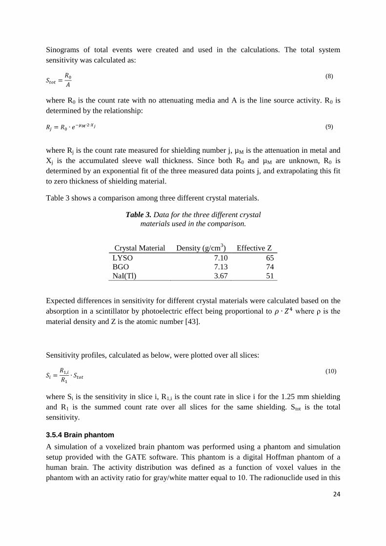
Table 3 shows a comparison among three different crystal materials.

Table 3. Data for the three different crystal

materials used in the comparison.

Crystal Material Density (g/cm3) Effective Z

LYSO 7.10 65

BGO 7.13 74

NaI(Tl) 3.67 51

Expected differences in sensitivity for different crystal materials were calculated based on the

absorption in a scintillator by photoelectric effect being proportional to where ρ is the

material density and Z is the atomic number [43].

Sensitivity profiles, calculated as below, were plotted over all slices:

(10)

where Si is the sensitivity in slice i, R1,i is the count rate in slice i for the 1.25 mm shielding

and R1 is the summed count rate over all slices for the same shielding. Stot is the total

sensitivity.

3.5.4 Brain phantom

A simulation of a voxelized brain phantom was performed using a phantom and simulation

setup provided with the GATE software. This phantom is a digital Hoffman phantom of a

human brain. The activity distribution was defined as a function of voxel values in the

phantom with an activity ratio for gray/white matter equal to 10. The radionuclide used in this

25

simulation was 18

F and the simulated acquisition time was 240 minutes. Images were

reconstructed with FBP using a Butterworth filter (cut-off frequency = 1.3 cm-1

, n = 5) from

sinograms with total, scatter and true events.

4 Results

All the results are given without uncertainties since only one simulation was run for each

calculation. In order to estimate standard deviations, several identical simulations would have

to be run.

4.1 Spatial resolution

The results from the spatial resolution measurements from the simulations are shown in Table

4 below. The results are measured for FWHM and FWTM for 1 cm off-center, 10 cm radial

and 10 cm tangential. The FWHM results are between 5.0 mm and 5.7 mm while those for

FWTM are between 8.1 mm and 9.4 mm.

Table 4. Results from the transversal

spatial resolution measurements.

Transversal Spatial

Resolution

FWHM

(mm)

FWTM

(mm)

1 cm 5.0 8.1

10 cm radial 5.4 9.4

10 cm tangential 5.7 8.8

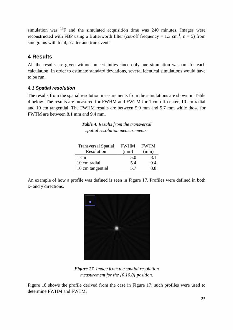
An example of how a profile was defined is seen in Figure 17. Profiles were defined in both

x- and y directions.

Figure 17. Image from the spatial resolution

measurement for the [0,10,0] position.

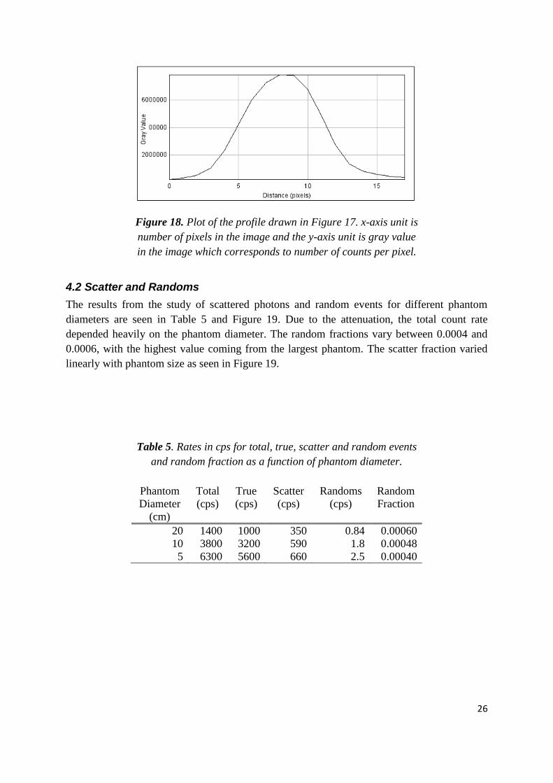
Figure 18 shows the profile derived from the case in Figure 17; such profiles were used to

determine FWHM and FWTM.

26

Figure 18. Plot of the profile drawn in Figure 17. x-axis unit is

number of pixels in the image and the y-axis unit is gray value

in the image which corresponds to number of counts per pixel.

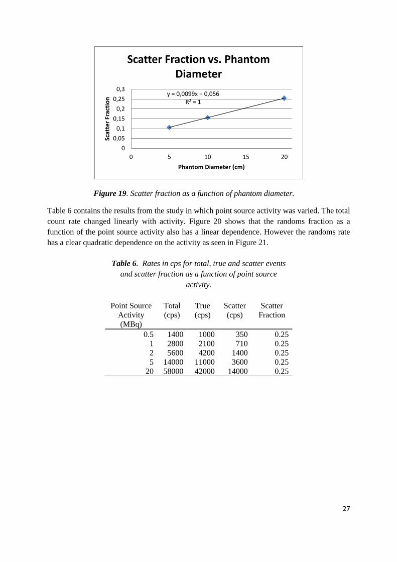
4.2 Scatter and Randoms

The results from the study of scattered photons and random events for different phantom

diameters are seen in Table 5 and Figure 19. Due to the attenuation, the total count rate

depended heavily on the phantom diameter. The random fractions vary between 0.0004 and

0.0006, with the highest value coming from the largest phantom. The scatter fraction varied

linearly with phantom size as seen in Figure 19.

Table 5. Rates in cps for total, true, scatter and random events

and random fraction as a function of phantom diameter.

Phantom

Diameter

(cm)

Total

(cps)

True

(cps)

Scatter

(cps)

Randoms

(cps)

Random

Fraction

20 1400 1000 350 0.84 0.00060

10 3800 3200 590 1.8 0.00048

5 6300 5600 660 2.5 0.00040

27

Figure 19. Scatter fraction as a function of phantom diameter.

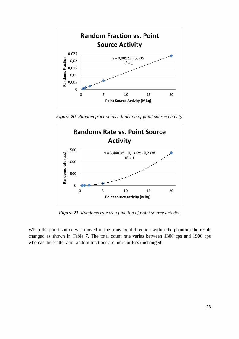
Table 6 contains the results from the study in which point source activity was varied. The total

count rate changed linearly with activity. Figure 20 shows that the randoms fraction as a

function of the point source activity also has a linear dependence. However the randoms rate

has a clear quadratic dependence on the activity as seen in Figure 21.

Table 6. Rates in cps for total, true and scatter events

and scatter fraction as a function of point source

activity.

Point Source

Activity

(MBq)

Total

(cps)

True

(cps)

Scatter

(cps)

Scatter

Fraction

0.5 1400

1000 350 0.25

1 2800

2100 710 0.25

2 5600

4200 1400 0.25

5 14000

11000 3600 0.25

20 58000

42000 14000 0.25

y = 0,0099x + 0,056 R² = 1

0

0,05

0,1

0,15

0,2

0,25

0,3

0 5 10 15 20

Scat

ter

Frac

tio

n

Phantom Diameter (cm)

Scatter Fraction vs. Phantom Diameter

28

Figure 20. Random fraction as a function of point source activity.

Figure 21. Randoms rate as a function of point source activity.

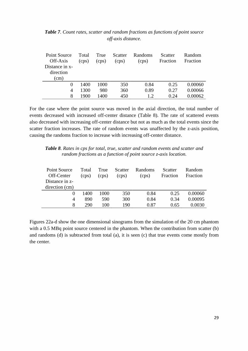
When the point source was moved in the trans-axial direction within the phantom the result

changed as shown in Table 7. The total count rate varies between 1300 cps and 1900 cps

whereas the scatter and random fractions are more or less unchanged.

y = 0,0012x + 5E-05 R² = 1

0

0,005

0,01

0,015

0,02

0,025

0 5 10 15 20

Ran

do

ms

Frac

tio

n

Point Source Activity (MBq)

Random Fraction vs. Point Source Activity

y = 3,4401x2 + 0,1312x - 0,2338 R² = 1

0

500

1000

1500

0 5 10 15 20

Ran

do

ms

rate

(cp

s)

Point source activity (MBq)

Randoms Rate vs. Point Source Activity

29

Table 7. Count rates, scatter and random fractions as functions of point source

off-axis distance.

Point Source

Off-Axis

Distance in x-

direction

(cm)

Total

(cps)

True

(cps)

Scatter

(cps)

Randoms

(cps)

Scatter

Fraction

Random

Fraction

0 1400 1000 350 0.84 0.25 0.00060

4 1300 980 360 0.89 0.27 0.00066

8 1900 1400 450 1.2 0.24 0.00062

For the case where the point source was moved in the axial direction, the total number of

events decreased with increased off-center distance (Table 8). The rate of scattered events

also decreased with increasing off-center distance but not as much as the total events since the

scatter fraction increases. The rate of random events was unaffected by the z-axis position,

causing the randoms fraction to increase with increasing off-center distance.

Table 8. Rates in cps for total, true, scatter and random events and scatter and

random fractions as a function of point source z-axis location.

Point Source

Off-Center

Distance in z-

direction (cm)

Total

(cps)

True

(cps)

Scatter

(cps)

Randoms

(cps)

Scatter

Fraction

Random

Fraction

0 1400 1000 350 0.84 0.25 0.00060

4 890 590 300 0.84 0.34 0.00095

8 290 100 190 0.87 0.65 0.0030

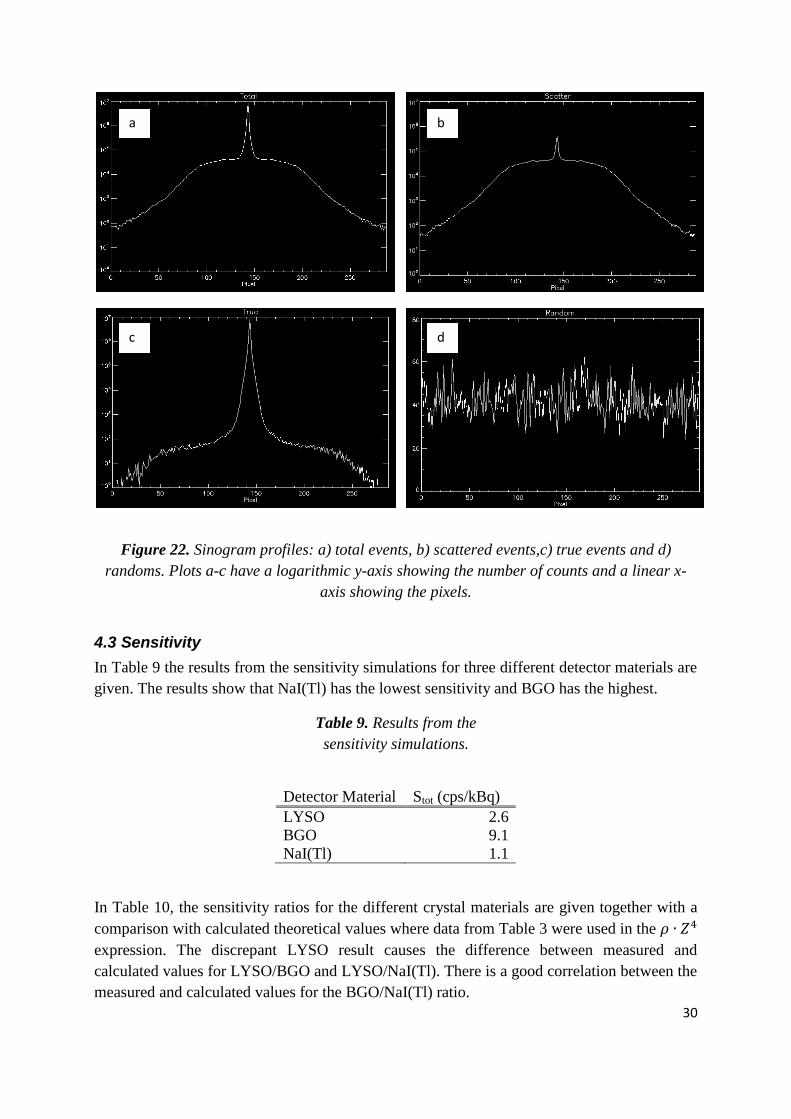
Figures 22a-d show the one dimensional sinograms from the simulation of the 20 cm phantom

with a 0.5 MBq point source centered in the phantom. When the contribution from scatter (b)

and randoms (d) is subtracted from total (a), it is seen (c) that true events come mostly from

the center.

30

Figure 22. Sinogram profiles: a) total events, b) scattered events,c) true events and d)

randoms. Plots a-c have a logarithmic y-axis showing the number of counts and a linear x-

axis showing the pixels.

4.3 Sensitivity

In Table 9 the results from the sensitivity simulations for three different detector materials are

given. The results show that NaI(Tl) has the lowest sensitivity and BGO has the highest.

Table 9. Results from the

sensitivity simulations.

Detector Material Stot (cps/kBq)

LYSO 2.6

BGO 9.1

NaI(Tl) 1.1

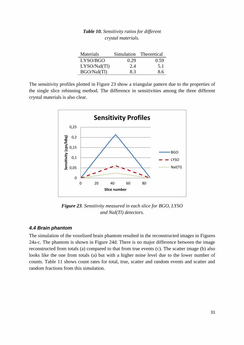
In Table 10, the sensitivity ratios for the different crystal materials are given together with a

comparison with calculated theoretical values where data from Table 3 were used in the

expression. The discrepant LYSO result causes the difference between measured and

calculated values for LYSO/BGO and LYSO/NaI(Tl). There is a good correlation between the

measured and calculated values for the BGO/NaI(Tl) ratio.

a

c d

b

31

Table 10. Sensitivity ratios for different

crystal materials.

Materials Simulation Theoretical

LYSO/BGO 0.29 0.59

LYSO/NaI(Tl) 2.4 5.1

BGO/NaI(Tl) 8.3 8.6

The sensitivity profiles plotted in Figure 23 show a triangular pattern due to the properties of

the single slice rebinning method. The difference in sensitivities among the three different

crystal materials is also clear.

Figure 23. Sensitivity measured in each slice for BGO, LYSO

and NaI(Tl) detectors.

4.4 Brain phantom

The simulation of the voxelized brain phantom resulted in the reconstructed images in Figures

24a-c. The phantom is shown in Figure 24d. There is no major difference between the image

reconstructed from totals (a) compared to that from true events (c). The scatter image (b) also

looks like the one from totals (a) but with a higher noise level due to the lower number of

counts. Table 11 shows count rates for total, true, scatter and random events and scatter and

random fractions from this simulation.

0

0,05

0,1

0,15

0,2

0,25

0 20 40 60 80

Sen

siti

vity

(cp

s/kB

q)

Slice number

Sensitivity Profiles

BGO

LYSO

NaI(Tl)

32

Figure 24. Voxelized brain phantom. The same slice is shown in four different versions: a)

image based on total events, b) scattered photons, c) true coincidences and d) the original

phantom image.

Table 11. Rates in cps for total, true, scatter and random events

and scatter and random fractions in Hoffman brain simulation.

Total

(cps)

True

(cps)

Scatter

(cps)

Randoms

(cps)

Scatter

Fraction

Random

Fraction

15000 14000 1700 33 0.11 0.0021

a b

c d

33

5 Discussion

In this work a model of Philips Gemini TF PET/CT system was built in GATE Monte Carlo

simulation software. Simulations of spatial resolution, different scatter measurements,

sensitivity and finally a voxelized phantom of a human brain were run.

GATE is a software for which it is easy to create complicated models of different

tomographic systems. A major problem in this work was to get detailed specifications about

the PET system used in the study. One specific issue that we chose not to take into account

was the system dead time because of its complex nature. However, with correct and detailed

information from the company it would be possible to build a realistic model.

The main disadvantage with GATE is that simulation time is very long, especially for

complex situations with voxelized phantoms and sources (for example one week on 60

computers for the voxelized brain phantom simulation). The other drawback is that the output

data files are large (the coincidence file was about 800 MB for a 4 minute simulation of 500

kBq point source in the ASCII format).

Compared to other existing dedicated Monte Carlo software (for example SimSET), GATE

seems to be able to handle more complex situations and therefore it is possible to do more

realistic simulations.

Other comparisons between an existing PET system and simulations of a model of that same

system have been done using GATE [5]. Results from that comparison show good agreement

between experimental measurements and simulated results.

5.1 Spatial resolution

Measurements of the transversal spatial resolutions where made according to the NEMA NU-

2 standard. The results are in agreement with those published by Surti et al. [39] (5.0 mm (4.8

mm), 5.4 mm (5.2 mm) and 5.7 mm (5.2 mm) respectively). The FWHM measurements from

these simulations are all slightly worse than the ones reported in the paper, but all are within

0.5 mm. This could be caused by the cubic interpolation that replaced proper image

reconstruction. The FWTM measurements from the GATE simulations are however better

(that is smaller) than published data from experimental measurements [39].

Spatial resolutions in the axial direction was not measured in this work because of the effects

of the single slice rebinning on the reconstructed images (due to intensity variations over

different angles in the sinograms and intensitiy “smearing” over several slices). Instead, all

sinogram slices where added together in a 2D sinogram and then reconstructed into one

image.

Results from the simulation of the spatial resolution were translated from number of pixels to

millimeters based on the fact that each detector element has a length of 4.0946 mm in the

transverse direction and that the elements in the sinograms are overlapping (Figure 12).

However, the “empty” sinogram elements corresponding to the gaps between the detector

34

blocks do not have the same size (only slightly smaller), and this fact was not considered in

the calculations of spatial resolution. This could possibly cause some minor distortions in the

images, but these effects were not seen. The empty sinogram elements cause streak artifacts in

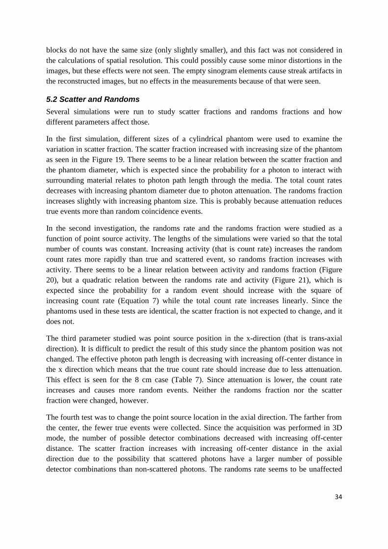
the reconstructed images, but no effects in the measurements because of that were seen.

5.2 Scatter and Randoms

Several simulations were run to study scatter fractions and randoms fractions and how

different parameters affect those.

In the first simulation, different sizes of a cylindrical phantom were used to examine the

variation in scatter fraction. The scatter fraction increased with increasing size of the phantom

as seen in the Figure 19. There seems to be a linear relation between the scatter fraction and

the phantom diameter, which is expected since the probability for a photon to interact with

surrounding material relates to photon path length through the media. The total count rates

decreases with increasing phantom diameter due to photon attenuation. The randoms fraction

increases slightly with increasing phantom size. This is probably because attenuation reduces

true events more than random coincidence events.

In the second investigation, the randoms rate and the randoms fraction were studied as a

function of point source activity. The lengths of the simulations were varied so that the total

number of counts was constant. Increasing activity (that is count rate) increases the random

count rates more rapidly than true and scattered event, so randoms fraction increases with

activity. There seems to be a linear relation between activity and randoms fraction (Figure

20), but a quadratic relation between the randoms rate and activity (Figure 21), which is

expected since the probability for a random event should increase with the square of

increasing count rate (Equation 7) while the total count rate increases linearly. Since the

phantoms used in these tests are identical, the scatter fraction is not expected to change, and it

does not.

The third parameter studied was point source position in the x-direction (that is trans-axial

direction). It is difficult to predict the result of this study since the phantom position was not

changed. The effective photon path length is decreasing with increasing off-center distance in

the x direction which means that the true count rate should increase due to less attenuation.

This effect is seen for the 8 cm case (Table 7). Since attenuation is lower, the count rate

increases and causes more random events. Neither the randoms fraction nor the scatter

fraction were changed, however.

The fourth test was to change the point source location in the axial direction. The farther from

the center, the fewer true events were collected. Since the acquisition was performed in 3D

mode, the number of possible detector combinations decreased with increasing off-center

distance. The scatter fraction increases with increasing off-center distance in the axial

direction due to the possibility that scattered photons have a larger number of possible

detector combinations than non-scattered photons. The randoms rate seems to be unaffected

35

by the change of point source position in the axial direction, but the randoms fraction

increased with increasing off-center distance (Table 8).

Profiles were plotted from the sinogram over the point source for one case. In a comparison

between total counts and true counts, the elimination of scattered events is obvious. However

the scattered events are not completely eliminated due to the fact that only photons which

have undergone Compton interaction in the phantom are considered in this study (Figure 22c).

Of course, Rayleigh interaction is also present (0.2%) [44], as well as interaction in the

detectors and shielding of the PET system etc. The random events are uniformly distributed

over the whole FOV as seen in Figure 22d.

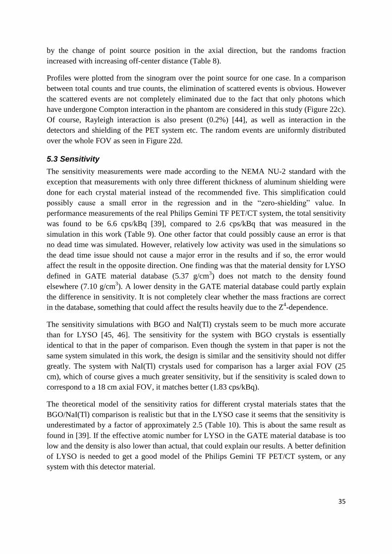
5.3 Sensitivity

The sensitivity measurements were made according to the NEMA NU-2 standard with the

exception that measurements with only three different thickness of aluminum shielding were

done for each crystal material instead of the recommended five. This simplification could

possibly cause a small error in the regression and in the “zero-shielding” value. In

performance measurements of the real Philips Gemini TF PET/CT system, the total sensitivity

was found to be 6.6 cps/kBq [39], compared to 2.6 cps/kBq that was measured in the

simulation in this work (Table 9). One other factor that could possibly cause an error is that

no dead time was simulated. However, relatively low activity was used in the simulations so

the dead time issue should not cause a major error in the results and if so, the error would

affect the result in the opposite direction. One finding was that the material density for LYSO

defined in GATE material database (5.37 g/cm3) does not match to the density found

elsewhere (7.10 g/cm3). A lower density in the GATE material database could partly explain

the difference in sensitivity. It is not completely clear whether the mass fractions are correct

in the database, something that could affect the results heavily due to the Z4-dependence.

The sensitivity simulations with BGO and NaI(Tl) crystals seem to be much more accurate

than for LYSO [45, 46]. The sensitivity for the system with BGO crystals is essentially

identical to that in the paper of comparison. Even though the system in that paper is not the

same system simulated in this work, the design is similar and the sensitivity should not differ

greatly. The system with NaI(Tl) crystals used for comparison has a larger axial FOV (25

cm), which of course gives a much greater sensitivity, but if the sensitivity is scaled down to

correspond to a 18 cm axial FOV, it matches better (1.83 cps/kBq).

The theoretical model of the sensitivity ratios for different crystal materials states that the

BGO/NaI(Tl) comparison is realistic but that in the LYSO case it seems that the sensitivity is

underestimated by a factor of approximately 2.5 (Table 10). This is about the same result as

found in [39]. If the effective atomic number for LYSO in the GATE material database is too

low and the density is also lower than actual, that could explain our results. A better definition

of LYSO is needed to get a good model of the Philips Gemini TF PET/CT system, or any

system with this detector material.

36

The sensitivity profiles have a clear triangular shape for all three crystal materials (Figure 23).

The values for the LYSO material do not correlate very well with published data, but this is

probably because of the overall error in the LYSO sensitivity simulation. The triangular shape

is explained by the single slice rebinning method used in the sinogram creation.

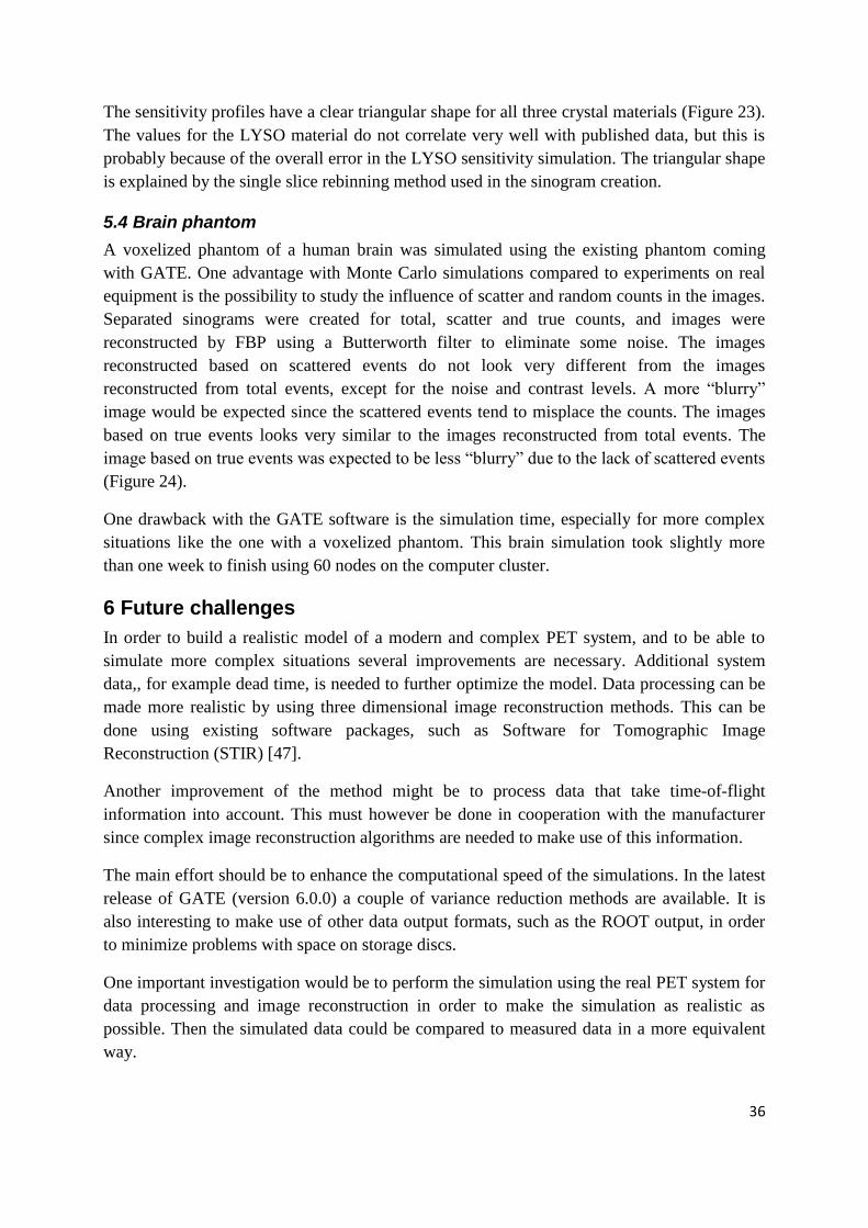
5.4 Brain phantom

A voxelized phantom of a human brain was simulated using the existing phantom coming

with GATE. One advantage with Monte Carlo simulations compared to experiments on real

equipment is the possibility to study the influence of scatter and random counts in the images.

Separated sinograms were created for total, scatter and true counts, and images were

reconstructed by FBP using a Butterworth filter to eliminate some noise. The images

reconstructed based on scattered events do not look very different from the images

reconstructed from total events, except for the noise and contrast levels. A more “blurry”

image would be expected since the scattered events tend to misplace the counts. The images

based on true events looks very similar to the images reconstructed from total events. The

image based on true events was expected to be less “blurry” due to the lack of scattered events

(Figure 24).

One drawback with the GATE software is the simulation time, especially for more complex

situations like the one with a voxelized phantom. This brain simulation took slightly more

than one week to finish using 60 nodes on the computer cluster.

6 Future challenges

In order to build a realistic model of a modern and complex PET system, and to be able to

simulate more complex situations several improvements are necessary. Additional system

data,, for example dead time, is needed to further optimize the model. Data processing can be

made more realistic by using three dimensional image reconstruction methods. This can be

done using existing software packages, such as Software for Tomographic Image

Reconstruction (STIR) [47].

Another improvement of the method might be to process data that take time-of-flight

information into account. This must however be done in cooperation with the manufacturer

since complex image reconstruction algorithms are needed to make use of this information.

The main effort should be to enhance the computational speed of the simulations. In the latest

release of GATE (version 6.0.0) a couple of variance reduction methods are available. It is

also interesting to make use of other data output formats, such as the ROOT output, in order

to minimize problems with space on storage discs.

One important investigation would be to perform the simulation using the real PET system for

data processing and image reconstruction in order to make the simulation as realistic as

possible. Then the simulated data could be compared to measured data in a more equivalent

way.

37

In the starting up of a new Bioimaging center at Lund University, a PET system for small

animal imaging has been purchased Nano-PET/CT (BioScan). Since this scanner is dedicated

to research it would be a good system to use for Monte Carlo simulations in cooperation with

the manufacturer.

Since this work began, a new release of GATE (version 6.0.0) became available with some

new features which could be used in the future.

Acknowledgments

Michael Ljungberg, Sven-Erik Strand and Lena Jönsson, Supervisors, Department of Medical

Radiation Physics, Lund University

John Palmer, Lund University Hospital

Kristina Norrgren, PhD Clinical Scientist, Philips Healthcare, Sweden

Suleman Surti, PhD, University of Pennsylvania, USA

James Bading, PhD Research Scientist, City of Hope Medical Center, USA

38

References

1. Gualdrini, G. and P. Ferrari, Monte Carlo evaluated parameters for internal dosimetry. Radiat Prot Dosimetry, 2007. 125(1-4): p. 157-60.

2. El Fakhri, G., et al., Absolute activity quantitation in simultaneous 123I/99mTc brain SPECT. J Nucl Med, 2001. 42(2): p. 300-8.

3. Frouin, V., et al., Correction of partial-volume effect for PET striatal imaging: fast implementation and study of robustness. J Nucl Med, 2002. 43(12): p. 1715-26.

4. Jan, S., et al., GATE: a simulation toolkit for PET and SPECT. Phys Med Biol, 2004. 49(19): p. 4543-61.

5. Lamare, F., et al., Validation of a Monte Carlo simulation of the Philips Allegro/GEMINI PET systems using GATE. Phys Med Biol, 2006. 51(4): p. 943-62.

6. M. E. Phelps, M.D., S. R. Cherry, PET: Physics, Instrumentation, and Scanners. 2006: Springer. 7. D. L. Baily, D.W.T., P. E. Valk, M. N. Maisey, Positron Emission Tomography: Basic Sciences.

2005: Springer. 8. Phelps, M.E., et al., Effect of positron range on spatial resolution. J Nucl Med, 1975. 16(7): p.

649-52. 9. de Jong, H., High Resolution PET imaging characteristics of 68Ga, 124I and 89Zr compared to 18F,

in IEEE Nuclear Science Symposium Conference Record. 2005. 10. Daube-Witherspoon, M.E. and G. Muehllehner, Treatment of axial data in three-dimensional

PET. J Nucl Med, 1987. 28(11): p. 1717-24. 11. Lewittt, R.M., G. Muehllehner, and J.S. Karpt, Three-dimensional image reconstruction for

PET by multi-slice rebinning and axial image filtering. Phys Med Biol, 1994. 39(3): p. 321-39. 12. Defrise, M., et al., Exact and approximate rebinning algorithms for 3-D PET data. IEEE Trans

Med Imaging, 1997. 16(2): p. 145-58. 13. Shepp, L.A. and Y. Vardi, Maximum likelihood reconstruction for emission tomography. IEEE

Trans Med Imaging, 1982. 1(2): p. 113-22. 14. Hudson, H.M. and R.S. Larkin, Accelerated image reconstruction using ordered subsets of

projection data. IEEE Trans Med Imaging, 1994. 13(4): p. 601-9. 15. Kinahan, P.E. and J.G. Rogers, Analytic 3d Image-Reconstruction Using All Detected Events.

Ieee Transactions on Nuclear Science, 1989. 36(1): p. 964-968. 16. Browne, J. and A.B. de Pierro, A row-action alternative to the EM algorithm for maximizing

likelihood in emission tomography. IEEE Trans Med Imaging, 1996. 15(5): p. 687-99. 17. Andreo, P., Monte Carlo techniques in medical radiation physics. Phys Med Biol, 1991. 36(7):

p. 861-920. 18. Ljungberg, M., Monte Carlo Calculations in Nuclear Medicine: Applications in Diagnostic

Imaging. 1998, Bristol: IOP Publishing. 19. Zaidi, H., Quantitative Analysis in Nuclear Medicine Imaging. 2005, New York: Springer. 20. Bai, B., et al., Evaluation of MAP image reconstruction with positron range modeling for 3D

PET. 2005 IEEE Nuclear Science Symposium Conference Record, Vols 1-5, 2005: p. 2686-2689 3054.

21. Dewaraja, Y.K., M. Ljungberg, and K.F. Koral, Characterization of scatter and penetration using Monte Carlo simulation in 131I imaging. J Nucl Med, 2000. 41(1): p. 123-30.

22. Bottigli, U., et al., Monte-Carlo Simulation and Experimental Tests on Bgo, Csf and Nai(Tl) Crystals for Positron Emission Tomography. Journal of Nuclear Medicine and Allied Sciences, 1985. 29(3): p. 221-227.

23. Derenzo, S.E., Monte-Carlo Calculations of the Detection Efficiency of Arrays of Nai(Tl), Bgo, Csf, Ge, and Plastic Detectors for 511-Kev Photons. Ieee Transactions on Nuclear Science, 1981. 28(1): p. 131-136.

24. Ljungberg, M. and S.E. Strand, Scatter and attenuation correction in SPECT using density maps and Monte Carlo simulated scatter functions. J Nucl Med, 1990. 31(9): p. 1560-7.

39

25. Poludniowski, G., et al., An efficient Monte Carlo-based algorithm for scatter correction in keV cone-beam CT. Phys Med Biol, 2009. 54(12): p. 3847-64.

26. Nelson, W.R., Hirayama, H. and Rogers, D. W. O., The EGS4 code system. 1985, Stanford Linear Accelerator Center.

27. Jordan, T.M., Its - the Integrated Tiger Series of Electron Photon Transport Codes Version-3.0 Cepxs Oneld Version-2.0 - a Discrete Ordinates Code Package for General One-Dimensional Coupled Electron-Photon Transport, and Recent Mcnp Developments - Comment. Ieee Transactions on Nuclear Science, 1993. 40(1): p. 71-72.

28. Forster, R.A. and T.N.K. Godfrey, Mcnp - a General Monte-Carlo Code for Neutron and Photon Transport. Lecture Notes in Physics, 1985. 240: p. 33-55.

29. Agostinelli, S., et al., GEANT4-a simulation toolkit. Nuclear Instruments & Methods in Physics Research Section a-Accelerators Spectrometers Detectors and Associated Equipment, 2003. 506(3): p. 250-303.

30. Lewellen, T., The SIMSET program, in Monte Carlo Calculation in Nuclear Medicine: Applications in Diagnostic Imaging, M. Ljungberg, Editor. 1998, Institute of Physics Publishing: Bristol. p. 77-92.

31. Ljungberg, M. and S.E. Strand, A Monte Carlo program for the simulation of scintillation camera characteristics. Comput Methods Programs Biomed, 1989. 29(4): p. 257-72.

32. Thompson, C.J., J. Morenocantu, and Y. Picard, Petsim - Monte-Carlo Simulation of All Sensitivity and Resolution Parameters of Cylindrical Positron Imaging-Systems. Physics in Medicine and Biology, 1992. 37(3): p. 731-749.

33. Reilhac, A., et al., PET-SORTEO: A Monte Carlo-based simulator with high count rate capabilities. Ieee Transactions on Nuclear Science, 2004. 51(1): p. 46-52.

34. Available from: http://www.opengatecollaboration.org. 35. GATE User Guide, Version 4.0.0. 2008. 36. Physics Reference Manual, geant4 9.2. 2008. 37. Buvat, I. and I. Castiglioni, Monte Carlo simulations in SPET and PET. Q J Nucl Med, 2002.

46(1): p. 48-61. 38. Philips Medical Systems, Gemini TF PET Specifications, XNGT-0210073, 2006. 39. Surti, S., et al., Performance of Philips Gemini TF PET/CT scanner with special consideration

for its time-of-flight imaging capabilities. J Nucl Med, 2007. 48(3): p. 471-80. 40. Surti S., University of Pennsylvania, 2009. 41. NEMA NU 2: Performance Measurements of Positron Emission Tomography. 2001, National

Electrical Manufacturers Association. 42. Available from: www.gridengine.org. 43. Van Eijk, C.W.E., Inorganic Scintillators in Positron Emission Tomography, in Radiation

Detectors for Medical Applications, S. Tavernier, Editor. 2006, Springer. p. 259-274. 44. Kawrakow, I., Efficient photon transport in positron emission tomography simulations using

VMC++, in Third McGill International Workshop. 2008, Journal of Physics: Conference Series 102.

45. Teras, M., et al., Performance of the new generation of whole-body PET/CT scanners: Discovery STE and Discovery VCT. Eur J Nucl Med Mol Imaging, 2007. 34(10): p. 1683-92.

46. Perkins, A.E., Performance Measurements of a Pixelated NaI(Tl) PET Scanner. IEEE Trans Nucl Sci, 2003. 50: p. 373-377.

47. Available from: http://stir.sourceforge.net.

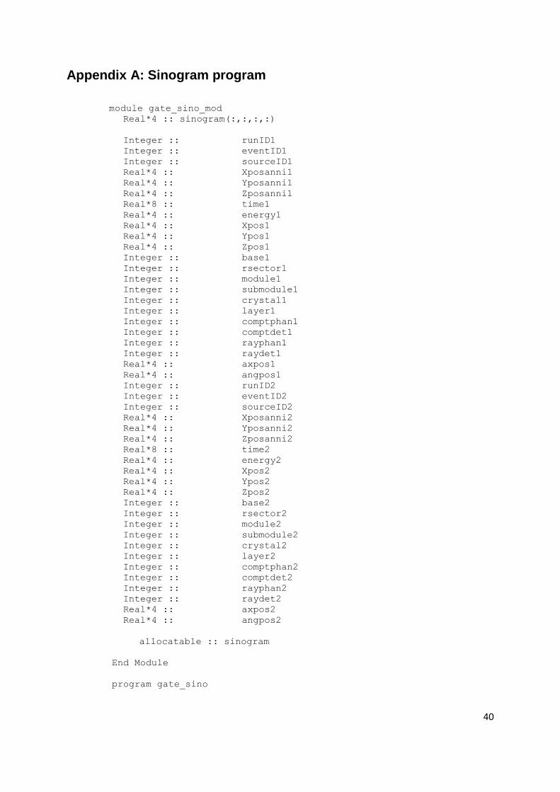
40

Appendix A: Sinogram program

module gate_sino_mod Real*4 :: sinogram(:,:,:,:)

Integer :: runID1

Integer :: eventID1

Integer :: sourceID1

Real*4 :: Xposanni1

Real*4 :: Yposanni1

Real*4 :: Zposanni1

Real*8 :: time1

Real*4 :: energy1

Real*4 :: Xpos1

Real*4 :: Ypos1

Real*4 :: Zpos1

Integer :: base1

Integer :: rsector1

Integer :: module1

Integer :: submodule1

Integer :: crystal1

Integer :: layer1

Integer :: comptphan1

Integer :: comptdet1

Integer :: rayphan1

Integer :: raydet1

Real*4 :: axpos1

Real*4 :: angpos1

Integer :: runID2

Integer :: eventID2

Integer :: sourceID2

Real*4 :: Xposanni2

Real*4 :: Yposanni2

Real*4 :: Zposanni2

Real*8 :: time2

Real*4 :: energy2

Real*4 :: Xpos2

Real*4 :: Ypos2

Real*4 :: Zpos2

Integer :: base2

Integer :: rsector2

Integer :: module2

Integer :: submodule2

Integer :: crystal2

Integer :: layer2

Integer :: comptphan2

Integer :: comptdet2

Integer :: rayphan2

Integer :: raydet2

Real*4 :: axpos2

Real*4 :: angpos2

allocatable :: sinogram

End Module

program gate_sino

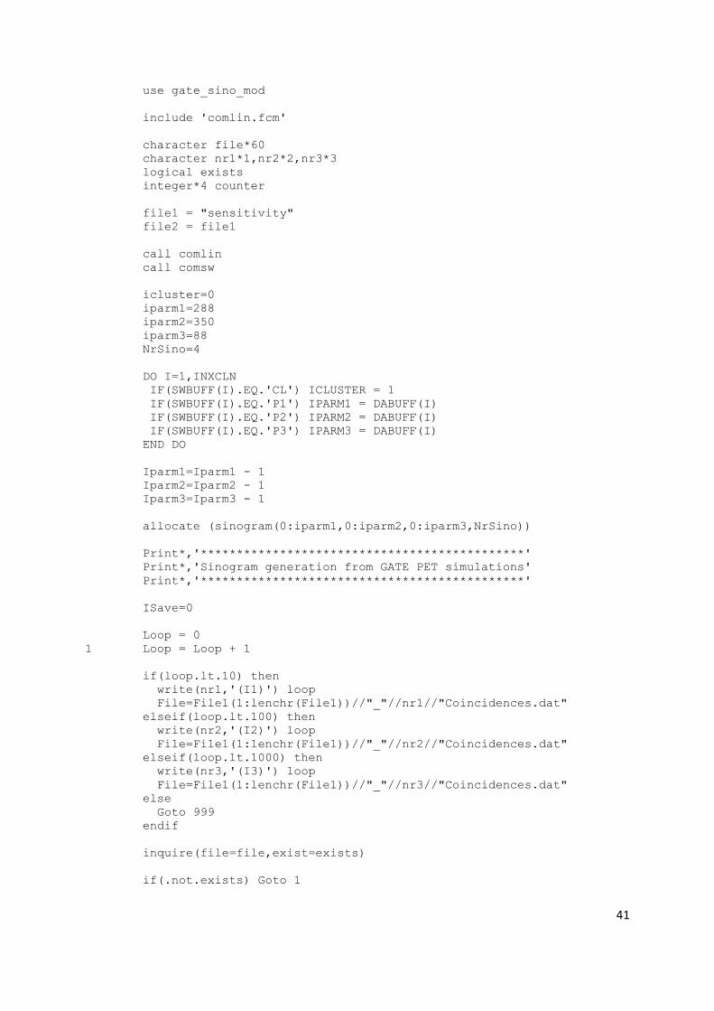
41

use gate_sino_mod

include 'comlin.fcm'

character file*60

character nr1*1,nr2*2,nr3*3

logical exists

integer*4 counter

file1 = "sensitivity"

file2 = file1

call comlin

call comsw

icluster=0

iparm1=288

iparm2=350

iparm3=88

NrSino=4

DO I=1,INXCLN

IF(SWBUFF(I).EQ.'CL') ICLUSTER = 1

IF(SWBUFF(I).EQ.'P1') IPARM1 = DABUFF(I)

IF(SWBUFF(I).EQ.'P2') IPARM2 = DABUFF(I)

IF(SWBUFF(I).EQ.'P3') IPARM3 = DABUFF(I)

END DO

Iparm1=Iparm1 - 1

Iparm2=Iparm2 - 1

Iparm3=Iparm3 - 1

allocate (sinogram(0:iparm1,0:iparm2,0:iparm3,NrSino))

Print*,'*********************************************'

Print*,'Sinogram generation from GATE PET simulations'

Print*,'*********************************************'

ISave=0

Loop = 0

1 Loop = Loop + 1

if(loop.lt.10) then

write(nr1,'(I1)') loop

File=File1(1:lenchr(File1))//"_"//nr1//"Coincidences.dat"

elseif(loop.lt.100) then

write(nr2,'(I2)') loop

File=File1(1:lenchr(File1))//"_"//nr2//"Coincidences.dat"

elseif(loop.lt.1000) then

write(nr3,'(I3)') loop

File=File1(1:lenchr(File1))//"_"//nr3//"Coincidences.dat"

else

Goto 999

endif

inquire(file=file,exist=exists)

if(.not.exists) Goto 1

42

open(1,file=file,err=99)

Isave=1 ! Någon händelse är registrerad dvs det blir ett sinogram

counter=0

2 counter = counter + 1

read(1,*,end=99,err=99)

x runID1,eventID1,sourceID1,Xposanni1,Yposanni1,Zposanni1,time1,

x energy1,Xpos1,Ypos1,Zpos1,base1,rsector1,module1,submodule1,

x crystal1,layer1,comptphan1,comptdet1,rayphan1,raydet1,axpos1,

x angpos1,runID2,eventID2,sourceID2,Xposanni2,Yposanni2,Zposanni2,

x time2,energy2,Xpos2,Ypos2,Zpos2,base2,rsector2,module2,

x submodule2,crystal2,layer2,comptphan2,comptdet2,rayphan2,

x raydet2,axpos2,angpos2

ring1 = Int(crystal1/23.)

a = crystal1 - ring1*23 + (rsector1)*25.

ring2 = Int(crystal2/23.)

b = crystal2 - ring2*23 + (rsector2)*25.

j = 2*ring1 - Int((ring1 - ring2))

k = Int((a-b+493))

l = Int(((a+b-698)/2.))

if (k.ge.0.and.k.le.iparm1.and.l.ge.0.and.l.le.iparm2) then

Call Store_sinogram(k,l,j)

endif

k = Int(b-a+493)

l = Int(((a+b-698)/2.))

if (k.ge.0.and.k.le.iparm1.and.l.ge.0.and.l.le.iparm2) then

Call Store_sinogram(k,l,j)

endif

k = Int(a-b-207)

l = Int(((a+b+2)/2.))

if (k.ge.0.and.k.le.iparm1.and.l.ge.0.and.l.le.iparm2) then

Call Store_sinogram(k,l,j)

endif

k = Int(b-a-207)

l = Int(((a+b+2)/2.))

if (k.ge.0.and.k.le.iparm1.and.l.ge.0.and.l.le.iparm2) then

Call Store_sinogram(k,l,j)

endif

Goto 2

99 Close(1)

print 888,file(1:lenchr(file)),counter

888 Format(' File processed: ',A,' Events:',I10)

Goto 1

999 If(Isave.gt.0) Then

Print*,' '

43

Do I=1,NrSino

If(I.eq.1) file2 = File1(1:lenchr(file1))//'.tota'

If(I.eq.2) file2 = File1(1:lenchr(file1))//'.true'

If(I.eq.3) file2 = File1(1:lenchr(file1))//'.scat'

If(I.eq.4) file2 = File1(1:lenchr(file1))//'.rand'

Open(2,file=file2,form='BINARY',Status='UNKNOWN')

write(2) sinogram(:,:,:,I)

Close(2)

Print*,'Sinogram in ',file2(1:lenchr(file2))

EndDo

Else

Print*,'No file(s) found'

Endif

Print*,'*********************************************'

End

SubRoutine Store_Sinogram(k,l,j)

use gate_sino_mod

sinogram(k,l,j,1)=sinogram(k,l,j,1)+1 !total

if(eventID1.eq.eventID2) then

if(comptphan1.eq.0) then

if(comptphan2.eq.0) then

sinogram(k,l,j,2)=sinogram(k,l,j,2)+1 !true

endif

endif

endif

if(comptphan1.gt.0.or.comptphan2.gt.0) then

sinogram(k,l,j,3)=sinogram(k,l,j,3)+1 !Scatter

endif

if(EventID1.ne.EventID2) then

sinogram(k,l,j,4)=sinogram(k,l,j,4)+1 !Random

endif

End

44

Appendix B: Reconstruction IDL-code

pro fbp

close,1

sinogram=fltarr(288,350,88)

openr,1,'C:\Users\Henrik\Desktop\spatial.total'

readu,1,sinogram

sinogram=sino(*,*,60)

matris=fltarr(288,288)

tomobild=fltarr(288,288,88)

ramp=[findgen(144),-findgen(144)+143]

rampnorm=abs(ramp/max(ramp))

butterworth=fltarr(288)

cutoff=75.

n=5.

butterworth=1./sqrt(1.+(ramp/cutoff)^(2*n))

for k=0,87 do begin

for j=0,349 do begin

fsinogram=fft(sinogram(*,j,k),-1)

sinogramf=fsinogram*ramp*butterworth

fsinogramf=fft(sinogramf,1)

for i=0,287 do begin

matris(i,*)=fsinogramf(i)

endfor

rotering=rot(matris,(360/700.)*j)

tomobild(*,*,k)=(tomobild(*,*,k)+rotering)

endfor

print,'done'

end