Monocular Visual Odometry for Robot Localization in LNG Pipes

Peter Hansen, Hatem Alismail, Peter Rander and Brett Browning

Abstract— Regular inspection for corrosion of the pipesused in Liquified Natural Gas (LNG) processing facilities iscritical for safety. We argue that a visual perception systemequipped on a pipe crawling robot can improve on existingtechniques (Magnetic Flux Leakage, radiography, ultrasound)by producing high resolution registered appearance maps ofthe internal surface. To achieve this capability, it is necessaryto estimate the pose of sensors as the robot traverses the pipes.We have explored two monocular visual odometry algorithms(dense and sparse) that can be used to estimate sensor pose.Both algorithms use a single easily made measurement of thescene structure to resolve the monocular scale ambiguity in theirvisual odometry estimates. We have obtained pose estimatesusing these algorithms with image sequences captured fromcameras mounted on different robots as they moved throughtwo pipes having diameters of 152mm (6”) and 406mm (16”),and lengths of 6 and 4 meters respectively. Accurate poseestimates were obtained whose errors were consistently lessthan 1 percent for distance traveled down the pipe.

I. INTRODUCTION

Corrosion of the pipes used in the sour gas processingstages of Liquified Natural Gas (LNG) facilities can lead tofailures that result in significant damage to the infrastructure,loss of product, and most importantly fatalities and seriousinjuries to humans. Detailed inspection of these pipes tomonitor corrosion rates is therefore a high priority.

In current industry practice, inspection is performed usingNon-Destructive sensors located external to the pipe tomeasure wall thickness, and/or by inserting sacrificial metalsamples into the pipe and measuring their loss of mate-rial rate. Example sensors include Magnetic Flux Leakage(MFL), ultrasound, and radiography (e.g. [1]). In either case,measurements can only be made in reachable locations. Pipesin LNG facilities are often densely packed and difficultto access, making complete coverage of the pipe networkexpensive and time consuming.

An alternative approach is to use a pipe crawling robotto measure all of the pipe surface thereby avoiding theneed for extensive, and potentially unreliable, predictivemodels. This approach has proven highly successful forinspecting gas pipelines, e.g. Pipe Inspection Guages (PIGs)1

and downstream networks [2], where wheel odometry and/orexpensive Inertial Motion Units (IMUs) are used when poseestimates are needed.

This paper was made possible by the support of an NPRP grant from theQatar National Research Fund. The statements made herein are solely theresponsibility of the authors.

Hansen and Browning are with the Qri8 lab, Carnegie Mellon University,Doha, Qatar phansen@qatar.cmu.edu. Alismail, Rander & Browningare with the Robotics Institute/NREC, Carnegie Mellon University, Pitts-burgh PA, USA, {halismai,rander,brettb}@cs.cmu.edu.

1http://www.geoilandgas.com/businesses/ge_oilandgas/en/prod_serv/serv/pipeline/en/inspection_services/index.htm

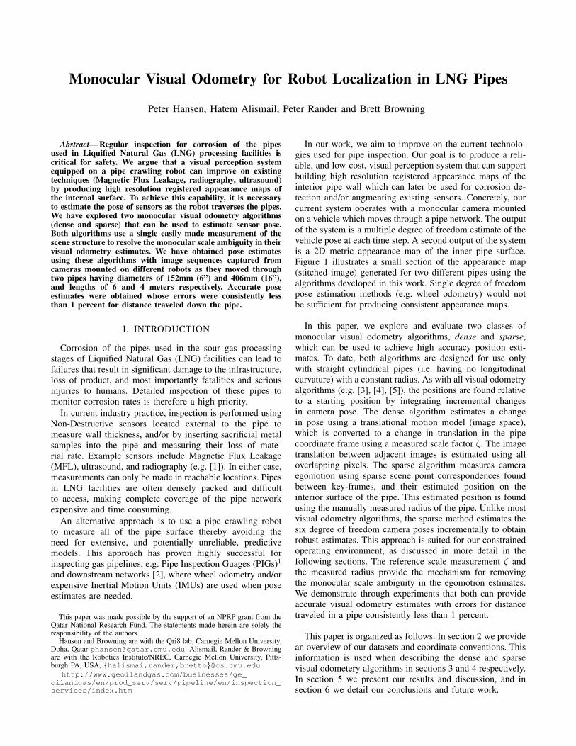
In our work, we aim to improve on the current technolo-gies used for pipe inspection. Our goal is to produce a reli-able, and low-cost, visual perception system that can supportbuilding high resolution registered appearance maps of theinterior pipe wall which can later be used for corrosion de-tection and/or augmenting existing sensors. Concretely, ourcurrent system operates with a monocular camera mountedon a vehicle which moves through a pipe network. The outputof the system is a multiple degree of freedom estimate of thevehicle pose at each time step. A second output of the systemis a 2D metric appearance map of the inner pipe surface.Figure 1 illustrates a small section of the appearance map(stitched image) generated for two different pipes using thealgorithms developed in this work. Single degree of freedompose estimation methods (e.g. wheel odometry) would notbe sufficient for producing consistent appearance maps.

In this paper, we explore and evaluate two classes ofmonocular visual odometry algorithms, dense and sparse,which can be used to achieve high accuracy position esti-mates. To date, both algorithms are designed for use onlywith straight cylindrical pipes (i.e. having no longitudinalcurvature) with a constant radius. As with all visual odometryalgorithms (e.g. [3], [4], [5]), the positions are found relativeto a starting position by integrating incremental changesin camera pose. The dense algorithm estimates a changein pose using a translational motion model (image space),which is converted to a change in translation in the pipecoordinate frame using a measured scale factor ζ. The imagetranslation between adjacent images is estimated using alloverlapping pixels. The sparse algorithm measures cameraegomotion using sparse scene point correspondences foundbetween key-frames, and their estimated position on theinterior surface of the pipe. This estimated position is foundusing the manually measured radius of the pipe. Unlike mostvisual odometry algorithms, the sparse method estimates thesix degree of freedom camera poses incrementally to obtainrobust estimates. This approach is suited for our constrainedoperating environment, as discussed in more detail in thefollowing sections. The reference scale measurement ζ andthe measured radius provide the mechanism for removingthe monocular scale ambiguity in the egomotion estimates.We demonstrate through experiments that both can provideaccurate visual odometry estimates with errors for distancetraveled in a pipe consistently less than 1 percent.

This paper is organized as follows. In section 2 we providean overview of our datasets and coordinate conventions. Thisinformation is used when describing the dense and sparsevisual odometery algorithms in sections 3 and 4 respectively.In section 5 we present our results and discussion, and insection 6 we detail our conclusions and future work.

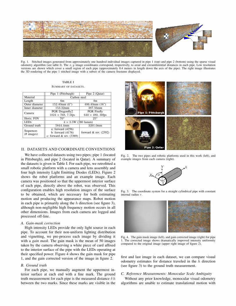
Fig. 1. Stitched images generated from approximately one hundred individual images captured in pipe 1 (top) and pipe 2 (bottom) using the sparse visualodometry algorithm (see table I). The x, y image coordinates correspond, respectively, to axial and circumferential distances in each pipe. Low resolutionversions are shown which cover a small region of each pipe (approximately 0.4 meters in length down the axis of the pipe). The right image illustratesthe 3D rendering of the pipe 1 stitched image with a subset of the camera frustums displayed.

TABLE ISUMMARY OF DATASETS.

Pipe 1 (Pittsburgh) Pipe 2 (Qatar)Material Carbon steelLength 6m 4mOuter diameter 152.40mm (6”) 406.40mm (16”)Inner diameter 153.32mm 387.56mm

Camera PGR Dragonfly2 PGR Firefly1024× 768, 7.5fps 640× 480, 30fps

Horiz. FOV 70◦ 25◦

LEDs 4× 3.5W (280 lumen)Ground truth 5844.4mm 3391.0mm

Sequences(# images)

a: forward (4256)forward & rev. (2392)b: forward (4176)

c: forward & rev. (3369)

II. DATASETS AND COORDINATE CONVENTIONSWe have collected datasets using two pipes; pipe 1 (located

in Pittsburgh), and pipe 2 (located in Qatar). A summary ofthe datasets is given in Table I. For each pipe, we retrofitted asmall robotic platform with a camera and lens assembly andfour high intensity Light Emitting Diodes (LEDs). Figure 2shows the robot platforms and an example image. Eachcamera was positioned so that the uppermost interior surfaceof each pipe, directly above the robot, was observed. Thisconfiguration enables high resolution images of the surfaceto be obtained, which are necessary for both estimatingmotion and producing the appearance maps. Robot motionin each pipe is primarily along the h direction (see figure 3),although non-negligible high frequency motion occurs in allother dimensions. Images from each camera are logged andprocessed off-line.

A. Gain-mask correctionHigh intensity LEDs provide the only light source in each

pipe. To account for their non-uniform lighting distributionand vignetting, we pre-process each image by dividing itwith a gain mask. The gain mask is the mean of 50 imagestaken by the camera observing a white piece of card affixedto the interior surface of the pipe with the LEDs operating attheir specified power. Figure 4 shows the gain mask for pipe1, and the gain corrected version of the image in figure 2.

B. Ground truthFor each pipe, we manually augment the uppermost in-

terior surface at each end with a fine mark. The groundtruth measurement for each pipe is the measured distance δ hbetween the two marks. Since these marks are visible in the

Fig. 2. The two pipes and robotic platforms used in this work (left), andexample images from each camera (right).

Fig. 3. The coordinate system for a straight cylindrical pipe with constantinternal radius r.

Fig. 4. The gain mask image (left), and gain corrected image (right) for pipe1. The corrected image shows dramatically improved intensity uniformitycompared to the original image (upper right image of figure 2).

first and last image in each dataset, we can compare visualodometry estimates for distance traveled in the h direction(see figure 3) to the ground truth measurement.

C. Reference Measurements: Monocular Scale AmbiguityWithout any prior knowledge, monocular visual odometry

algorithms are unable to estimate translational motion with

metric units. The dense and sparse algorithms both use areference scale measurement to resolve this ambiguity. Thedense algorithm uses a scale measurement ζ (pixels/meter),which relates a change in pixel coordinates in undistorted2

perspective images to a metric change in position in the pipecoordinate frame. The scale factor ζ is obtained by imaginga reference pattern fixed to the surface of the pipe, andthen finding the ratio of the pixel distance between pointsin the pattern to their known metric distance. This processis completed before collecting datasets. The reference scalemeasurements that were obtained for pipe 1 and pipe 2 areζ = 10.47× 103 and ζ = 7.16× 103 respectively.

The sparse monocular algorithm enforces that all worldpoints observed in the images lie on the interior surfaceof a straight cylindrical pipe with constant radius. Hence,we manually measure the inner diameters of each pipe (seeTable I, and [6] for details).

D. Coordinate ConventionsReferring to figure 3, we define X = (X,Y, h)T ∈ R3

as the coordinate of a world point in the pipe’s coordinateframe. The coordinate of a scene point, constrained to lie onthe interior surface of the pipe, can be parameterized as:

X =(r cosφ r sinφ h

)T, (1)

where φ = tan−1(Y/X). The pose Pt of the camera relativeto the pipe at time t is written as:

Pt =

[R −RC0T 1

], (2)

where R is a 3×3 rotation matrix, and C is a 3×1 Euclideanposition vector of the camera with respect to the origin of thepipe. The pose Pt defines the transform of a world point withcoordinate Xi, in the pipe coordinate frame, to coordinateYi in the camera coordinate frame:(

YTi 1

)T= Pt

(XT

i 1)T. (3)

III. DENSE MONOCULARThe dense monocular algorithm uses direct, or pixel-based,

image registration (alignment) to estimate camera egomo-tion [7], [8]. We use a two degrees of freedom parametricmodel [9], whereby adjacent images It−1, It are related bya single δx = (δx, δy)T pixel shift (image translation):

It(x) = It−1(x− δx). (4)

We set the initial camera pose P0 as3:

P0 =

[R−1 C0T 1

]−1=

0 1 0 CX

0 0 1 CY

1 0 0 00 0 0 1

−1

. (5)

The change in pose Q = P−1 between adjacent images,measured in the pipe coordinate frame of reference, is

Q =

[I3×3 δC0T 1

]−1, δC =

1

ζ(δy, 0, δx)T . (6)

2Using the Matlab Calibration Toolbox http://www.vision.caltech.edu/bouguetj/calib_doc/

3The camera’s principal axis is in the direction of the pipe’s y-axis, andthe camera’s x axis is in the direction of the pipe’s h axis.

The scale factor ζ discussed in section 2 allows the imagetranslation δx to be converted to a change in camera pose δC,in the pipe coordinate frame, with metric units. The unknownoffsets CX and CY in (5) could be manually measured ifdesired. However, they have no influence on the estimate ofthe distance the robot travels in the h direction down the pipe.To estimate the image translation δx, we use a full-searchmethod followed by an iterative model-based refinement.

A. Full-searchAn initial integer estimate of the image translation δx

is obtained by sliding one of the images over the otheron a 2D grid in image space. The objective is to find thealignment (image translation δx) that minimizes a functionof image dissimilarity. In this work, we use the Sum ofAbsolute Difference (SAD) normalized by the area of overlapto measure the quality of registration.

B. Iterative model-based refinementIn an attempt to improve upon the initial integer estimate

of δx obtained using full-search, we proceed to use theiterative model-based registration framework proposed by [9]for sub-pixel refinement. The translational motion δx be-tween image pairs is approximated iteratively using a Gauss-Newton refinement process to minimize the Sum of SquaredDifferences (SSD) between adjacent images, normalized bythe area of overlap (see [9] for details). Iteration continuesuntil convergence, or an empirically selected maximum num-ber of times is exceeded.

Iterative registration schemes are prone to converge in alocal minima if the overlap between images is small. Obtain-ing an initial estimate for δx using the full search methodguarantees, in most cases, that the iterative refinement willconverge to a more accurate estimate of the correct motion.

IV. SPARSE MONOCULARThe sparse monocular algorithm estimates camera ego-

motion based on the changes in positions of sparse keypointcorrespondences in adjacent images. These changes are typi-cally referred to as the sparse optical flow, and are used as thebasis for many monocular visual odometry algorithms [3],[10]. However, most visual odometry algorithms are designedto operate in unstructured environments where the relativeEuclidean coordinates of scene points cannot be derivedfrom a single image; they must be triangulated from pairsor sequences of images [11]. As discussed, we constrain thecamera to lie within a straight cylindrical pipe with a fixed,and known, radius r. The Euclidean coordinate Xi of anypixel in an image can therefore be derived given the radius rand camera pose Pn. Camera egomotion is estimated usingthe derived world point coordinates X of the sparse keypointcorrespondences. Using the world point coordinates enablesthe camera egomotion to be estimated with metric units oftranslation. Hence, the monocular scale ambiguity is avoided.

A. Obtaining Scene Point CorrespondencesA region-based Harris corner detector [12] is used to

identify keypoints in the original (distorted) gain-correctedgray-scale images4. Each image is divided into an equally

4Adjacent images contain minimal scale change, and we have found noadvantages using scale-invariant keypoints (e.g. SIFT [13]).

spaced 6× 8 grid, and the 20 most salient keypoints in eachcell retained after non-maxima suppression of the saliencyvalues using a 7 × 7 pixel wide window — the saliencyis the Harris ‘cornerness’ score. A region-based scheme isused to ensure that there is a uniform distribution of key-points throughout the image. Sub-pixel keypoint positions areobtained using a two-dimensional quadratic interpolation ofthe Harris cornerness score based on the scheme developedin [13]. A 128-dimensional SIFT descriptor [13] is thenevaluated for each keypoint from the gray-scale intensityvalues within a fixed sized region surrounding it. Since thecameras used have been calibrated, the pixel position xi

of each keypoint is mapped to a spherical coordinate ηi,xi 7→ ηi, which defines a ray in space originating from thecamera center.

Given any two images, corresponding keypoints are foundusing the ambiguity metric [13] for the SIFT descriptors witha mutual consistency check. However, the correspondencebetween every adjacent pair of images are not used to esti-mate motion since many are separated by only a few pixelsdifference. We use a method similar to that of Mouragnon etal [14] and Tardif et al [10] to automatically select only keyframes (images) that are used to obtain the visual odometryestimates. Starting with the first image I0 in the sequence,we keep finding the correspondences between image I0 andIj , where Ij is the jth image in the sequence. When thenumber of correspondences between image I0 and Ij fallsbelow a threshold, or the median magnitude of the sparseoptical flow vectors is above some threshold, the set ofcorrespondences between images I0 and Ij−1 are kept, andimages I0 and Ij−1 are assigned a camera pose Pn=0 andPn=1 respectively. This process is then repeated starting atimage Ij−1, and continued for the remainder of the sequence.The images In used to compute the camera egomotion arethe key-frames. We attempt to remove any outliers in the setof correspondences between key frames using RANSAC [15]and the five-point algorithm in [16].

B. Euclidean coordinates of scene pointsRecall that the image coordinate xi of any keypoint can

be mapped to a spherical coordinate ηi using the cameracalibration parameters. We parameterize a world point in thecamera coordinate frame, which is constrained to lie on theinterior surface of a pipe with radius r, as Yi = κi ηi, whereκi is a scalar. From (3), Xi = R−1 Yi + C, which is thecoordinate of the point in the world (pipe) coordinate frame.Letting R = [R1 R2 R3], and referring to figure 3 and (1),the coordinate Xi = (X,Y, h)T must satisfy the constraint:

r2 = X2 + Y 2 (7)

= (κi R1 ηi + CX)2+ (κi R2 ηi + CY )

2. (8)

Expanding (8) produces a quadratic in κi, which has onepositive and one negative solution if the camera is inside thepipe. The positive solution is correct since the point must bein front of the perspective camera, and defines the Euclideanscene point coordinate Yi = κi ηi, where Xi = R−1 Yi+C.

C. Visual Odometry EstimationSix degree of freedom (6-DOF) motion estimates are

obtained using a number of steps:

1) Initial one degree of freedom (1-DOF) estimation.2) Optimization of initial camera position.3) Six degree of freedom (6-DOF) refinement.

Before discussing each of these steps, it is important tointroduce the global index g for each world point. Assumethat the same world point is detected in multiple images,and the keypoint correspondences found between key framesenables us to identify that these keypoints do in fact belongto the same world point. If the pose P is know for each of theimages, then the coordinate X of this point could be derivedfrom any of the images using the procedure described in theprevious section. We assign this world point a global index g,Xg , and store each of the j estimates of its position obtainedfrom different images, Xg

j .1) Initial one degree of freedom estimation: Since the

camera motion in a straight cylindrical pipes was constrainedprimarily to a change in translation δh down the pipe, theinitial estimate of each camera pose Pn+1 is

Pn+1 =

[Rn −Rn (Cn + δC)0T 1

], (9)

where δC = (0, 0, δh)T , which has only a single degree offreedom δ h. The estimate for δh is obtained using all rele-vant prior information in the sequence, here the coordinatesX of all the world points derived before key-frame n+ 1.

For an estimate of Pn+1, we derive the coordinates ofthe world points using the method described previously. De-note these points X. A non-linear optimization (Levenberg-Marquardt) is used to find the estimate of δ h in equation 9which minimizes the error

ε =∑g

∑j

[Xg

j − Xgj

]2, (10)

where∑

j is the summation for all j estimates of theworld point with global index g. We could have projectedthe images coordinates X to the current image, and thenminimized the distance to their observed (detected) pixelpositions. However, the derived positions X, X all have anapproximately equal uncertainty5, and we have found themethod used to provide satisfactory results.

2) Optimization of initial camera position: We perform abatch optimization, using the first ten key-frames, to improveupon the initial manually measured estimate for Cn=0 (wekeep Ch = 0 for the first key-frame).

The optimization used does not minimize the errors be-tween the scene point coordinates X. The reason is thatthe coordinates of all of these points change during a batchoptimization, and it is not clear how a suitable normalizationfactor can be selected — moving the camera closer to thepipe surface minimizes the dispersion of the scene pointsand the magnitude of the errors. For this reason, the errorminimized is defined in image space with respect to thecoordinates of the keypoints detected in the original images.

The estimate for P0 is set to the same initial pose used bythe dense algorithm, see (5), using the manually measuredvalues for CX and CY . For each iteration, a 1-DOF estimate

5This applies for the camera configuration used, which has a narrow fieldof view, and assuming a (fixed scale) Gaussian uncertainty of the detectedkeypoint positions.

for each of the ten cameras P0,··· ,9 is obtained, and the worldcoordinates X of all the corresponding keypoints are foundfrom their image coordinates x. These points can then bemapped to image coordinates x in any of the other imageswhere they were found. The error ε′ minimized is defined inimage space as

ε′ =∑g

∑j

[xgj − xg

j

]2, (11)

where, again,∑

j is the summation for all j estimates of theworld point with global index g. Note that xg and xg mayappear in two or more images in the set.

3) Six degree of freedom refinement: The initial 1-DOFestimate is used to obtain a reasonably accurate initialestimate of camera pose. We refine the pose estimates usinga 6-DOF model and a sliding window scheme. After eacha = τN key frames, where τ is any integer and N = 50 is aconstant, the 6-DOF refinement for the previous 2N framesis implemented. This implementation is performed separatelyfor each frame in the window, and no ‘batch’ optimizationof all the frames is used.

For frame Pk, where 1 ≤ k ≤ a, the coordinates Xfor each of the correspondences in the image are foundfor a given six degrees of freedom estimate of Pk —these points are no longer assumed to belong to the setof world points X. The optimized 6-DOF estimate is theone which minimizes (10). The non-linear optimization isimplemented using Levenberg-Marquardt, where the camerarotation R is parameterized using quaternions. This processis implemented sequentially from the first to last image inthe window. Since this method limits the degree by whichthe pose can change, it is run for an empirically selectednumber of times, which in the following experiments is two.

D. Selection of incremental addition of degrees of freedomWhen an initial estimate of a camera’s pose Pn is obtained,

only information from the previous frames can be used.However, during the 6-DOF sliding window optimization,a camera’s pose Pn is optimized using information from allframes. Attempting to estimate a camera’s 6-DOF pose usingonly information from previous frames proved unreliableand inaccurate — this is the same reason why we don’tuse the five-point algorithm to obtain an initial egomotionestimate. One reason for this is the difficulty in reliablydecoupling rotational and translational motion when usingnarrow field of view (i.e. typical perspective) cameras [17],particularly when: there are minimal depth discontinuities inthe scene [18]; there are small changes in camera rotationand/or translation [19], [20]; the focus of expansion orcontraction is outside the camera’s field of view [17]. The lasttwo factors in particular exist for our camera configuration(see [6] for details). Using information from all framesto estimate the 6-DOF motion enabled significantly morereliable and accurate results to be obtained.

V. RESULTS AND DISCUSSIONA. Results

Visual odometry results were obtained, for the datasetssummarized in table I, using the dense and sparse algorithms.The estimates of the distance traveled down the axis of the

TABLE IIDENSE AND SPARSE ALGORITHM RESULTS. ALL PERCENTAGES ARE

ABSOLUTE VALUES. SEE TABLE I FOR GROUND TRUTH.

Dataset Metric Dense SparsePipe 1a error mm -9.0 (0.154%) 17.9 (0.306%)Pipe 1b error mm 42.4 (0.725%) 16.9 (0.289%)

Pipe 1cFwd. error mm 8.7 (0.149%) 7.5 (0.128%)Rev. error mm -21.1 (0.361%) 3.5 (0.060%)Tot. error mm 29.8 (0.255%) 4.0 (0.034%)

Pipe 2Fwd. error mm 28.4 (0.838%) 7.1 (0.209%)Rev. error mm -99.0 (2.919%) 20.7 (0.619%)Tot. error mm 127.4 (1.879%) -13.6 (0.201%)

pipe versus the ground truth measurements are summarizedin table II (the errors are the ground truth values minus theabsolute estimated change δh of camera pose). The absolutepercentage errors are also recorded in the table. For thedatasets (Pipe 1c, Pipe 2) where the robot moves forwarddown the pipe, and then reverses in the opposite direction,the total (’loop closure’) error is ε = fwd. err− rev. err. Thetotal absolute percentage error is then

ε(%) = 100×|fwd. err−rev. err|/ (2× ground truth) . (12)

B. DiscussionThe results in table II show that the dense and sparse

algorithms are capable of finding accurate visual odometryestimates with respect to distance traveled down the pipe,with errors consistently less than 1 percent. Note that nei-ther of the pipes used contained any significant geometricdeviations from the straight cylindrical, uniform radius pipeassumption used by both the dense and sparse algorithms(e.g. longitudinal curvature, change in radius, non-circularprofile). We would expect less accurate visual odometryresults to be obtained if they were introduced and theexperiments repeated. Overall, the sparse algorithm performsmarginally better than the dense algorithm. A number offactors which influence the accuracy of the visual odometryestimates are discussed here.

1) Gain-correction: Non-uniform light distribution in theimages severely impacts the accuracy of the dense egomotionestimates since the pixels themselves (intensity and gradient)are used to estimate the image translation δx. When usingthe original (not gain-corrected) images, we observed the fullsearch estimates of δx incorrectly converging on solutionswhich align the non-uniform light patterns in the images.Our gain correction procedure is only approximate, andcannot account for specularities in the images — we onlyobserved small specularities in some of the images, and havesince used polarizing materials to limit them. As a resultthe gain corrected images may contain some non-uniformlighting which limits the accuracy of the dense egomotionestimates. Any remaining non-uniform lighting in the gaincorrected images will negatively impact the accuracy ofkeypoint localization, and as a result the accuracy of thesparse egomotion estimates. However, non-uniform lightingeffects the sparse egomotion estimates far less than that bywhich it effects the dense egomotion estimates.

2) Inherent motion model assumptions: The densemonocular algorithm assumes that image pairs are relatedby an image shift δx, which corresponds to a 2-DOF changein camera position (i.e. translation) in the pipe. Referring to

−3500 −3000 −2500 −2000 −1500 −1000 −500 0−15−10

−505

1015

h position (mm)

X p

ositio

n (

mm

)

−3500 −3000 −2500 −2000 −1500 −1000 −500 0−3

−2

−1

01

h position (mm)

Y p

ositio

n (

mm

)

Fig. 5. The estimate of the camera position C = (X,Y, h)T in pipe 2 obtained using the sparse algorithm: robot traveling forward (blue), and robottraveling in reverse (red). The high frequency change in position X is due primarily to the robot design.

figure 5, the Y coordinate of the camera changes significantlywhen traveling in the reverse direction – the robot ‘climbed’up the side of the pipe by rotating about the pipe’s axis.The dense monocular algorithm is unable to correctly modelthis motion. As a result, the pose estimates for pipe 2 (rev)obtained using the dense algorithm are poor in comparisonto the 6-DOF estimate found using the sparse algorithm.

3) Pipe diameter and camera angle of view: Referringto table I, pipe 1 has a smaller diameter than pipe 2, andthe horizontal angle of view of the lens used with pipe 1 isgreater than that for pipe 2. This means that, compared topipe 2, the images in the pipe 1 datasets exhibit a greaterdegree of foreshortening, and the distance of the world pointsfrom the camera in pipe 1 are less.

Foreshortening negatively impacts the dense monocularegomotion estimates since the algorithm assumes that thecamera is observing a planar scene (translational model).Although foreshortening presents challenges during keypointdetection and matching using the sparse algorithm, it haslittle impact when finding the sparse egomotion estimates.

The ability to image scene points at a small distance froma high resolution camera, using a large angle of view lens,is desirable for visual odometry applications [17], [18], [20].Therefore, we would expect the accuracy of the sparse visualodometry estimates obtained for pipe 1 to be better than thoseobtained for pipe 2. The results obtained support this claim.

VI. CONCLUSIONS AND FUTURE WORKWe have investigated two monocular visual odometry

algorithms, dense and sparse, that are designed to estimatecamera pose in a straight cylindrical pipe. This is a firststep towards a visual perception system for LNG pipesinspection. Importantly, knowledge of the scene structure(i.e. a straight cylindrical pipe with constant radius) is usedby both to resolve the monocular scale ambiguity in theirvisual odometry estimates. The algorithms were evaluatedon different datasets taken in different pipes. In the exper-iments presented, both were able to estimate camera posewithin 1% accuracy of the ground truth. However, the moresophisticated sparse algorithm was able the outperform thedense algorithm due to its ability to model 6-DOF motion,and its relative invariance to non-uniform image lighting.In ongoing work we are exploring different stereo cameracamera configurations which may be used to produce highresolution, and high accuracy, estimates of the internal 3Dstructure of pipes.

VII. ACKNOWLEDGMENTSThe authors gratefully acknowledge the contribution of

Mohamed Mustafa (CMQ) and Joey Gannon (RI-NREC) indeveloping the dataset collection hardware.

REFERENCES

[1] J. Nestleroth and T. Bubenik, “Magnetic flux leakage (MFL) tech-nology for natural gas pipeline inspection,” Battelle, Report NumberGRI-00/0180 to the Gas Research Institute, Tech. Rep., 1999.

[2] H. Schempf, “Visual and nde inspection of live gas mains using arobotic explorer,” JFR, vol. Winter, 2009.

[3] D. Nister, O. Naroditsky, and J. Bergend, “Visual odometry for groundvehicle applications,” JFR, vol. 23, no. 1, pp. 3–20, January 2006.

[4] M. Maimone, Y. Cheng, and L. Matthies, “Two years of visualodometry on the mars exploration rovers,” JFR, vol. 24, no. 3, pp.169–186, March 2007.

[5] A. Levin and R. Szeliski, “Visual odometry and map correlation,” inCVPR, June 2004, pp. 611–618.

[6] P. Hansen, H. Alismail, P. Rander, and B. Browning, “Towards a visualperception system for pipe inspection: Monocular visual odometry,”Robotics Institute, Carnegie Mellon University, Pittsburgh, PA, Tech.Rep. CMU-RI-TR-10-22 / CMU-CS-QTR-104, July 2010.

[7] R. Szeliski, “Image alignment and stitching: A tutorial,” in Founda-tions and Trends in Computer Graphics and Vision. Now PublishersInc., 2006.

[8] A. Ardeshir, 2-D and 3-D Image Registration. Wiley & Sons, 2005.[9] J. Bergen, P. Anandan, K. Hanna, and R. Hingorani, “Hierarchical

model-based motion estimation,” in ECCV’92, 1992, pp. 237–252.[10] J.-P. Tardif, Y. Pavlidis, and K. Daniilidis, “Monocular visual odometry

in urban environments using an omnidirectional camera,” in Proceed-ings IROS, 2008, pp. 2531–2538.

[11] R. Hartley and A. Zisserman, Multiple View Geometry in ComputerVision, 2nd ed. Cambridge University Press, 2003.

[12] C. Harris and M. Stephens, “A combined corner and edge detector,”in Proceedings Fourth Alvey Vision Conference, 1988, pp. 147–151.

[13] D. Lowe, “Distinctive image features from scale-invariant keypoints,”IJCV, vol. 60, no. 2, pp. 91–110, 2004.

[14] E. Mouragnon, M. Lhuillier, M. Dhome, F. Dekeyser, and P. Sayd,“Real time localization and 3D reconstruction,” in CVPR, 2006.

[15] M. A. Fischler and R. C. Bolles, “Random sample consensus: Aparadigm for model fitting with applications to image analysis andautomated cartography,” Comms. of the ACM, pp. 381–395, 1981.

[16] D. Nister, “An efficient solution to the five-point relative pose prob-lem,” PAMI, vol. 26, no. 6, pp. 756–770, June 2004.

[17] J. Gluckman and S. Nayar, “Ego-motion and omnidirectional cam-eras,” in CVPR, 1998, pp. 999–1005.

[18] K. Daniilidis and H.-H. Nagel, “The coupling of rotation and trans-lation in motion estimation of planar surfaces,” in CVPR, June 1993,pp. 188–193.

[19] D. Nister, “Reconstruction from uncalibrated sequences with a hierar-chy of trifocal tensors,” in ECCV, 2000, pp. 649–663.

[20] J. Neumann, C. Fermuller, and Y. Aloimonos, “Eyes form eyes: Newcameras for structure from motion,” in Proceedings Workshop onOmnidirectional Vision (OMNIVIS), 2002.