wheeled-robot’s velocity updating and odometry- based ... · wheeled-robot’s velocity updating...
TRANSCRIPT

i
CENTRO DE INVESTIGACIÓN Y DE ESTUDIOS
AVANZADOS DEL INSTITUTO POLITÉCNICO NACIONAL
Department of Computer Science
Wheeled-Robot’s velocity updating and odometry-
based localization by navigating on outdoor terrains
Thesis presented by
M. en C. Farid García Lamont
For the Degree of
PhD in Computer Science
Thesis advisor: José Matías Alvarado Mentado
México, D.F. November 2010


i
CENTRO DE INVESTIGACIÓN Y DE ESTUDIOS
AVANZADOS DEL INSTITUTO POLITÉCNICO NACIONAL
Departamento de Computación
Wheeled-Robot’s velocity updating and odometry-
based localization by navigating on outdoor terrains
Tesis que presenta
M. en C. Farid García Lamont
Para obtener el Grado de
Doctor en Ciencias en Computación
Director de la Tesis: José Matías Alvarado Mentado
México, D.F. Noviembre 2010


Abstract
This thesis addresses the velocity updating of wheeled-robots regarding the terrains’ textures
and slopes -beyond detection and avoidance of the obstacles as most current works do.
Terrain appearance recognition enables the wheeled-robots to adapt their velocity such that,
1) as speedy as possible it safely navigates, and 2) precision on vehicle localization using
odometry-based methods is improved.
Human drivers make the velocity adjusting using an estimation of the terrain’s average
appearance. When a human driver finds a new texture, he uses his experience to learn how
rough the texture is, and then sets the car’s velocity. A fuzzy neural network that allows for
mimicking the human experience by driving vehicles in outdoor terrains is deployed.
The fuzzy neural network metaclassifies data about the textures and slopes’ inclination
of terrains hence to compute the wheeled-vehicle navigation velocity; in addition, combined
with the gradient method it enables the vehicle path planning. The experimental tests
show improved robot’s performance with velocity updating: the wheels of the robot slip
very less, thus the wheeled-robot odometry errors are lower too hence precision of robot
self-localization is improved. Advances are both with respect to traveled distance and with
respect to the spent time for making the travel.
The first set of tests are performed using a small wheeled-robot which adjusts velocity
while navigating on surfaces with different classes of textures such as ground, grass, and
stones paving. The second set of tests are done using images of roads of ground, concrete,
asphalt, and loose stones, which are video filmed from a real car driven at less than 60 km/hr
of velocity; by applying the present approach the required time/distance ratio to smoothly
velocity change is granted.

Given the vehicle recognition/navigation implementation is simple and computationally
low-cost, and simulation results of the velocity updating of a car, suggests that the proposed
approach can be scaled to real vehicles.
2

Resumen
En esta tesis se aborda el ajuste de velocidad de un robot con ruedas tomando en cuenta
las texturas y pendientes de los terrenos -mas alla de la deteccion y evasion de obstaculos
como en la mayorıa de los trabajos actuales se enfocan. El reconocimiento de la apariencia
de los terrenos permite a los robots con ruedas adaptar su velocidad tal que, 1) se mueva
tan rapido como pueda sin que la navegacion llegue a ser peligrosa, 2) se mejora la precision
en la localizacion del vehıculo al emplear metodos basados en odometrıa.
En el manejo de vehıculos, los conductores humanos ajustan la velocidad haciendo una
estimacion de la apariencia promedio del terreno. Cuando un conductor humano encuentra
una nueva textura, este emplea su experiencia para estimar que rugosa es la textura, y ası
establecer la velocidad del carro. Se emplea una red neuronal difusa con la cual se imita la
experiencia humana para el manejo de vehıculos en terrenos exteriores.
Una red neuronal difusa metaclasifica la informacion de las texturas y de la inclinacion
de las pendientes de los terrenos para calcular la velocidad de navegacion del robot; ademas,
combinado con el metodo del gradiente este permite la planeacion de trayectorias del vehıculo.
Los resultados experimentales muestran una mejora en el desempeno del robot con el ajuste
de velocidad: el deslizamiento de las ruedas del robot es menor, de esta manera el error sub-
yacente de la odometrıa es menor y de aquı que se mejora la precision en el auto localizacion
del robot. Las mejoras son con respecto a la distancia recorrida y al tiempo de recorrido del
robot.
Un primer conjunto de experimentos son realizados empleando un pequeno robot con
ruedas el cual ajusta su velocidad mientras navega en superficies con diferentes clases de tex-
turas tales como tierra, tierra con pasto y adoquın. El segundo conjunto de experimentos son
realizados empleando imagenes de caminos con tierra, concreto, asfalto y piedras sueltas, las
cuales son video grabadas desde un vehıculo real conducido a menos de 60 km/hr; al aplicar
el presente enfoque el tiempo/distancia requerido para ajustar la velocidad suavemente es

garantizado.
Dados que la implementacion del reconocimiento y navegacion es sencilla y computa-
cionalmente barato, y los resultados de la simulacion del ajuste de velocidad de un carro, se
sugiere que el enfoque propuesto puede ser escalado a vehıculos de mayor tamano.
4

Dedicatorias
A mi esposa e hija Estella Esparza Zuniga y Estrella Faride Garcıa Esparza
A mis padres Irma Lamont Sanchez y Armando Garcıa Hernandez
A mis hermanos Jair Garcıa Lamont y Harim Garcıa Lamont
A mis abuelos Aurelio Garcıa y Raquel Sanchez

Agradecimientos
La conclusion de esta tesis es el resultado del esfuerzo y apoyo de varias personas. Pensar
y asumir que fue resultado de una sola persona, seria un acto de soberbia. A continuacion
menciono a los actores responsables.
Agradezco al Consejo Nacional de Ciencia y Tecnologıa (CONACyT) por la beca No.
207029 otorgada de febrero de 2007 a agosto de 2009, y por la extension de beca otorgada
en el periodo septiembre de 2009 a agosto de 2010.
Agradezco al Deutcher Akademischer Austauschdienst (DAAD) por la beca, con codigo
A/07/97585, otorgado para mi estancia academica en la Universidad Libre de Berlın en
Alemania en el verano de 2007.
Agradezco al Instituto de Ciencia y Tecnologıa del Distrito Federal (ICyTDF) por el
apoyo economico otorgado para presentar mi articulo en el International Conference on
Informatics in Control (ICINCO), en Funchal - Madeira, Portugal.
Agradezco al CINVESTAV-IPN por el apoyo economico para la inscripcion y asistencia
a los congresos ICINCO y al Mexican Conference on Pattern Recognition (MCPR), en los
cuales me fueron aceptados y presentados mis artıculos. Y en general por todos los servicios
proporcionados.
Agradezco al Dr. Raul Rojas por permitirme hacer la estancia academica con su equipo
de trabajo FU-Fighters y FUmanoids.
Agradezco al Dr. Aldo Mirabal y al Dr. Ernesto Tapia por su hospitalidad, apoyo, guıa,
incluso por compartir suenos, durante mi estancia en Berlın, Alemania (zie je in Berlijn,
gezondheid! ).
Agradezco al Ing. Jose Ramon Garcıa Alvarado por su valiosısima ayuda en la imple-
mentacion del algoritmo de plantacion de trayectorias, el cual fue muy importante para la
obtencion de varios resultados que se presentan en esta tesis. Eres una de las personas con
mas talento que he conocido, aprovechalo!!!

Agradezco al Dr. Hebertt Sira Ramırez, Dr. Leopoldo Altamirano Robles, Dr. Luis
Enrique Sucar Succar, Dr. Adriano de Luca Pennacchia, Dr. Debrup Chakraborty y al
Dr. Jorge Buenabad Chavez por haber aceptado ser mis sinodales y por sus observaciones
realizadas durante la revision de este trabajo.
Agradezco al Dr. Matıas Alvarado Mentado por aceptar ser mi asesor y por su direccion
durante mi estancia en el Departamento de Computacion.
Agradezco al Dr. Gustavo Nunez Esquer y a la Universidad Politecnica de Pachuca por
autorizar los permisos laborales para que pudiera estudiar el doctorado.
Agradezco a la Dra. Palmira Rivera por su enorme apoyo para que yo pudiera comenzar
a estudiar el doctorado.
Agradezco a las secretarias Felipa Rosas, Flor Cordova, Sofia Reza y Erika Rıos por su
gran ayuda en el papeleo, reserva de boletos de avion y demas tramites burocraticos que a
veces hacen ver al doctorado como un juego de ninos. A ellas mi mas sincero agradecimiento.
Al Ing. Arcadio Morales por facilitarme el equipo necesario para la realizacion de mis
experimentos.
Al Dr. Jair Cervantes le agradezco su solidaridad, ayuda y consejos, y por tenerme la
confianza y fe, que incluso a veces ni yo mismo tengo.
A los companeros del CINVESTAV que me acompanaron durante mi doctorado.
Agradezco a los Sopranos (Angel, Ernesto, Arturo e Israel) por su honesta amistad. Ojala
pronto volvamos a poner a rodar otra vez al tren.
Finalmente, pero mas importantes, agradezco a mi bella esposa Estella Esparza por su
paciencia, apoyo, por aguantarme, por sus consejos y enorme comprension todo este tiempo,
y por haberme dado una hermosa hija, Estrellita. A ellas dos, todo mi amor.
A mis papas, Irma Lamont y Armando Garcıa por su apoyo, y carino incondicional. Pero
mas importante, por haberme ensenado a pensar y mostrarme la diferencia entre pensar y
aprender. A ellos, todo mi respeto y carino.
A mis abuelos Raquel Sanchez y Aurelio Garcıa por haber iniciado el proyecto, el cual
7

he tenido la fortuna de continuar y la responsabilidad de mantener y de agrandarlo.
... gracias totales!!!...
8

Citas
• Cuando se inicia y desencadena una batalla lo que importa no es tener la razon, sino
conseguir la victoria. Adolfo Hitler
• Prefiero ser el peor de los mejores que el mejor de los peores. Kurt Cobain
• Si aceptas las expectativas de los demas, especialmente las negativas, entonces nunca
cambiaras el resultado. Michael Jordan
• Somos lo que recordamos. Francisco Martın Moreno
• A veces el mejor regalo es la gratificacion de no volverte a ver. Dr. Gregory House

10

Contents
1 Introduction 19
1.1 Problem statement . . . . . . . . . . . . . . . . . . . . . . . . . . . . . . . . 21
1.2 The solution proposal . . . . . . . . . . . . . . . . . . . . . . . . . . . . . . . 23
1.3 Objectives . . . . . . . . . . . . . . . . . . . . . . . . . . . . . . . . . . . . . 27
1.4 Contributions . . . . . . . . . . . . . . . . . . . . . . . . . . . . . . . . . . . 28
2 Mobile Robot Navigation 29
2.1 Wheeled-robot navigation . . . . . . . . . . . . . . . . . . . . . . . . . . . . 30
2.2 Outdoor terrain recognition . . . . . . . . . . . . . . . . . . . . . . . . . . . 38
3 Texture Recognition 43
3.1 State of the art . . . . . . . . . . . . . . . . . . . . . . . . . . . . . . . . . . 44
3.1.1 Edge density . . . . . . . . . . . . . . . . . . . . . . . . . . . . . . . 46
3.1.2 Auto-Correlation function . . . . . . . . . . . . . . . . . . . . . . . . 46
3.1.3 Fourier spectral analysis . . . . . . . . . . . . . . . . . . . . . . . . . 47
3.1.4 Histogram features . . . . . . . . . . . . . . . . . . . . . . . . . . . . 47
3.1.5 Gray level difference method . . . . . . . . . . . . . . . . . . . . . . . 48
3.1.6 Co-occurrence analysis . . . . . . . . . . . . . . . . . . . . . . . . . . 48
3.1.7 Fractal analysis . . . . . . . . . . . . . . . . . . . . . . . . . . . . . . 49
3.1.8 Textural energy . . . . . . . . . . . . . . . . . . . . . . . . . . . . . . 50
11

3.1.9 Spatial/Frequency methods . . . . . . . . . . . . . . . . . . . . . . . 51
3.1.10 Structural approaches to texture analysis . . . . . . . . . . . . . . . . 51
3.1.11 Local Binary Patterns . . . . . . . . . . . . . . . . . . . . . . . . . . 52
3.1.12 Advanced Local Binary Patterns with Rotation Invariance . . . . . . 53
3.2 Appearance-Based Vision . . . . . . . . . . . . . . . . . . . . . . . . . . . . 55
3.3 Experiments . . . . . . . . . . . . . . . . . . . . . . . . . . . . . . . . . . . . 58
3.4 Methods comparison . . . . . . . . . . . . . . . . . . . . . . . . . . . . . . . 59
4 Velocity Updating 63
4.1 Neural networks for roughness recognition . . . . . . . . . . . . . . . . . . . 65
4.2 Fuzzy logic for roughness estimation . . . . . . . . . . . . . . . . . . . . . . 66
4.3 Neuro-Fuzzy approach . . . . . . . . . . . . . . . . . . . . . . . . . . . . . . 68
4.4 Fuzzy neural network architecture . . . . . . . . . . . . . . . . . . . . . . . . 71
5 Experiments and Simulations for Velocity Updating 79
5.1 Terrain recognition supporting navigation . . . . . . . . . . . . . . . . . . . 80
5.2 Simulations at real car velocities . . . . . . . . . . . . . . . . . . . . . . . . . 85
5.3 Cycle time: vision processing and velocity updating . . . . . . . . . . . . . . 90
6 Odometry-Based Localization Improvement 93
6.1 Autonomous wheeled-robots localization . . . . . . . . . . . . . . . . . . . . 94
6.2 Odometry . . . . . . . . . . . . . . . . . . . . . . . . . . . . . . . . . . . . . 97
6.3 The navigation algorithm . . . . . . . . . . . . . . . . . . . . . . . . . . . . . 99
6.3.1 Path planning and velocity updating . . . . . . . . . . . . . . . . . . 100
6.3.2 The gradient method . . . . . . . . . . . . . . . . . . . . . . . . . . . 102
6.4 Experiments . . . . . . . . . . . . . . . . . . . . . . . . . . . . . . . . . . . . 106
12

7 Discussion 113
7.1 Beyond the personal velocity updating . . . . . . . . . . . . . . . . . . . . . 113
7.2 Odometry-based methods improving . . . . . . . . . . . . . . . . . . . . . . 114
7.2.1 Scalability . . . . . . . . . . . . . . . . . . . . . . . . . . . . . . . . . 114
7.2.2 Autonomous Navigation . . . . . . . . . . . . . . . . . . . . . . . . . 115
8 Conclusions and Contributions 119
A CUReT Texture Images for Experiments 121
B Published Articles 123
B.1 Journals in ISI Web (Journal Citation Report) . . . . . . . . . . . . . . . . . 123
B.2 Proceedings conference indexed in ISI Web . . . . . . . . . . . . . . . . . . . 123
13

14

List of Figures
1.1 Wheeled-robot on an outdoor terrain with different classes of textures and
soft irregularities . . . . . . . . . . . . . . . . . . . . . . . . . . . . . . . . . 23
1.2 Autonomous navigation with velocity updating diagram. For velocity estima-
tion it is employed data from both texture classification and slopes’ inclination.
The robot moves along the planned path at the estimated velocity; while the
robot moves, the images of the terrain are acquired and the inclination of the
slopes are measured; this information is processed and the velocity is updated,
if there are any changes in terrain roughness . . . . . . . . . . . . . . . . . . 26
2.1 Ackerman wheel configuration . . . . . . . . . . . . . . . . . . . . . . . . . . 34
2.2 Two-wheeled bicycle arrangement . . . . . . . . . . . . . . . . . . . . . . . . 34
2.3 Three-wheel ominidirectional robot . . . . . . . . . . . . . . . . . . . . . . . 35
2.4 Two-wheel differential-drive robot . . . . . . . . . . . . . . . . . . . . . . . . 36
3.1 Local Binary Patterns . . . . . . . . . . . . . . . . . . . . . . . . . . . . . . 53
4.1 Block diagram of the proposed approach for velocity updating . . . . . . . . 69
4.2 Slope detection employing two infrared sensors. The infrared rays extend until
them “touch” a terrain irregularity, thus, a virtual right triangle is drawn,
where the rays play the role of cathetus and the irregularity as hypotenuse.
The angle is computed with simple trigonometric operations . . . . . . . . . 70
15

4.3 Fuzzy neural network architecture. The FNN has five layers, the first layer
has two inputs, the slope inclination and the texture class, the second layer
sets the terms of input membership variables, the third one sets the terms of
the rule base, the fourth sets the term of output membership variables, and
in the fifth layer, the output is the robot’s velocity . . . . . . . . . . . . . . . 72
4.4 Texture roughness membership function . . . . . . . . . . . . . . . . . . . . 73
4.5 Slopes membership function . . . . . . . . . . . . . . . . . . . . . . . . . . . 73
4.6 Velocity membership function . . . . . . . . . . . . . . . . . . . . . . . . . . 73
5.1 Wheeled-robot employed for testing . . . . . . . . . . . . . . . . . . . . . . . 80
5.2 Car vision/recognition system. The camera must process the next 5-meter
road segment before the vehicle passes over. That is, when the vehicle moves
the first 5-meter stretch, the computer processes the image of the posterior
5-meter stretch. When the second stretch processing is finished, the vehicle
would have started to move in the second stretch. This cycle is successively
repeated . . . . . . . . . . . . . . . . . . . . . . . . . . . . . . . . . . . . . . 91
6.1 Robot navigation competences . . . . . . . . . . . . . . . . . . . . . . . . . . 94
6.2 Scheme integration of path planning and velocity estimation algorithms for
autonomous navigation . . . . . . . . . . . . . . . . . . . . . . . . . . . . . . 100
6.3 Flow diagram of the navigation algorithm, where the path planning and ve-
locity updating algorithms are integrated to work harmonized for autonomous
navigation on outdoor terrains . . . . . . . . . . . . . . . . . . . . . . . . . . 102
6.4 Outdoor terrain employed for autonomous navigation testing . . . . . . . . . 106
6.5 Typical robot path, dot line, during navigation on the surface shown in Figure
6.4. Black dots represent the two obstacles located in the straight line between
the start and goal locations of the robot . . . . . . . . . . . . . . . . . . . . 107
16

List of Tables
1.1 Examples of outdoor textures . . . . . . . . . . . . . . . . . . . . . . . . . . 24
2.1 The four basic wheel types . . . . . . . . . . . . . . . . . . . . . . . . . . . . 32
3.1 Performance of texture recognition methods . . . . . . . . . . . . . . . . . . 59
4.1 If-Then rules of the FNN’s inference system . . . . . . . . . . . . . . . . . . 74
5.1 Velocities estimated under the neuro-fuzzy approach by employing the ABV,
ALBPRI, LBP and FCS methods for texture classification. The velocities are
estimated in meter per minute units . . . . . . . . . . . . . . . . . . . . . . . 83
5.2 Videotaped textures in outdoor terrains from the perspective of a driver in a
car . . . . . . . . . . . . . . . . . . . . . . . . . . . . . . . . . . . . . . . . . 87
5.3 Velocity updating results by employing the texture classes shown in Table 5.2 89
6.1 Results obtained from the set of experiments of autonomous navigation on
the terrain shown in Figure 6.4 . . . . . . . . . . . . . . . . . . . . . . . . . 109
A.1 CUReT images employed for experiments . . . . . . . . . . . . . . . . . . . . 122
17

18

Chapter 1
Introduction
Navigation with vehicles in unknown environments is an easy task for humans, but very
difficult for robots. Giving autonomy to robots is a topic that has been extensively studied,
although still there is much to do. For autonomous navigation in outdoor terrains, the robot
must be endowed with the ability to interpret data acquired from its environment so as to
plan and follow trajectories from its current location to the desired location, considering the
features of the terrains. Most autonomous navigation works have focused on the problem
of recognition and avoidance of obstacles; however, so far, almost no attention has been
placed on the recognition of terrains’ textures and irregularities, and how they affect the
performance and safety of robots during navigation.
Current algorithms in robots’ systems for outdoor navigation or exploration have mainly
focused on the recognition and avoidance of obstacles such as stones, earth mounds [1], or
other vehicles [2]. On navigation paths the obstacles are identified in GPS images [3], or
taken by the robot’s sensors system [4], [5], such that images allow the autonomous robots’
conduction to avoid collisions [6].
Actually, by moving on outdoors, autonomous robots should avoid obstacles now and
again to maintain fine velocity control, and this issue has received broad attention [7]. How-
19

ever, the robot’s velocity control regarding the terrain features has been much less attended
and it is a weakness for efficient and safe navigation nowadays. The right navigating velocity
regarding the terrain features is a requisite to keep robots away from risks of falling and
sliding due to surface slopes or smash textures [8], the vehicle velocity must be updated
according to the terrain features in order to guarantee robots safe navigation.
For wheeled-robots navigation on terrains, it is necessary to have required information
about the surface features such that automated safe navigation is ensured. One of those
features on which this work focuses is the surface roughness where the vehicle is moving on.
The robot’s velocity during real navigation depends on the terrain roughness; moreover, the
robot integrity depends on the right velocity of the robot while navigating through terrain,
it is likely that the robot has an accident if it moves in ground at the same speed as it does
on asphalt, therefore, this would not be convenient for a smooth and efficient navigation.
Outdoors autonomous robots are particularly relevant when employed in planet missions.
The terrain difficulties like dusty ground, rocks and slopes of Solar System planets -like Mars-
require in these exploration missions the usage of robots with the highest degree of autonomy
to overcome the difficulties for controlling the robots from the remote Earth. The Spirit and
Opportunity rovers spent 26 minutes to receive/send instructions from/to the Earth [9], [10].
The risk to lose information is huge due to unpredicted circumstances, so the autonomy on
robot navigation abilities is most valuable in these out of Earth missions.
In Earth exploration missions, where human life could be in danger, autonomous rovers
are required for explosive landmines search [11], deep sea exploration [12], or to determine the
eruption risk when exploring active volcano craters [13], as well others. In these dangerous
circumstances, the high autonomy of robots strengthens the robotic support to human safety.
On the other hand, by extending the robots’ abilities to recognize the terrains’ features
and then, accordingly, update the velocity while navigating, the usage of the robots’ energy
and computing resources would improve as well as the autonomy would be strengthen.
20

1.1 Problem statement
Navigation with vehicles in unknown environments is an easy task for humans, but very
difficult for robots. Robotic autonomous navigation throughout outdoor terrains is highly
complex. Detection of obstacles to avoid collisions, as well as the terrain features information
acquisition to prevent sliding are both required. The information of environment needs to
be quickly and accurately processed by the robot’s navigation systems for a right displacing.
Besides, when needed information from human remote controllers is not promptly available,
the autonomous robots should be equipped for convenient reactions, particularly in front
of unpredicted circumstances. All these are tasks and actions which demand many compu-
tational resources. However, any autonomous robot has limited resources. Thereafter, for
autonomous navigation, the equation combining robot’s robust capacities to make complex
and specialized actions and the low resources use in real time need to be harmonized. This
is the current challenge.
Among the related works of navigation in rough terrains, they are mainly concentrated
on the detection and avoidance of obstacles [14], [15], [16], [17]. So far, it has not been
addressed comprehensively the problem of autonomous navigation where the robot velocity
is updated according to the terrains’ roughness, i.e. depending on the irregularities and
textures of terrains.
The recognition of terrains’ textures is not an issue that has been widely studied and
applied to autonomous navigation. There are also some works in which present texture
recognition methods of terrains. For instance, vibration-based [18], [19] and laser-ray [7],
[20], [21] methods have shown high performance; but with vibration-based methods the
robot classifies the textures until it is moving over them; and the laser-ray methods are
computationally expensive because of the intensive real-time processing of the huge quantity
data sampled from the terrains.
On the other hand, for autonomous navigation the robot must determine self-localization
21

within its environment; robot localization becomes a matter of determining coordinates and
orientation on a two dimensional floor-plan. For wheeled-robots, odometry is frequently
used to do this task [22]; but odometry inevitably accumulates errors due to causes as the
diameters of the wheels are not equal or poor wheel alignment, wheel slippage, among others
[23].
Several works have managed to reduce the odometry errors by modeling errors from the
readings of the encoders coupled to the robot wheels to improve the calculation of the robot
location. Their results show reduction of odometry errors; but all these works are assisted by
landmarks [24], laser beams [25] and artificial vision [26], among other tools [27] to compute
the robots’ location on the terrain.
So far, the reduction of wheel slippage has not been attended for the purpose of improving
the odometry-based localization of wheeled-robots.
Thus, the problems that arise are:
• To adjust the velocity of a mobile wheeled-robot while it autonomously navigates
on outdoor terrains, which contain different classes of textures, obstacles and soft
irregularities.
• The velocity setting must be performed remotely, i.e. the robot must detect and
classify soft irregularities and textures before the robot passes on them, so that the
robot disposes enough time to react and set its velocity according to the terrains’
characteristics.
• Reduce the slippage of robots’ wheels to improve the localization of the robots using
odometry-based methods.
Figure 1.1 shows a wheeled-robot moving through a surface with irregularities and dif-
ferent classes of textures; where the wheeled-robot must adjust its velocity according to the
terrains’ features in order to avoid slidings and collisions against obstacles.
22

Figure 1.1: Wheeled-robot on an outdoor terrain with different classes of textures and soft
irregularities
In this thesis, a soft irregularity is defined as a slope with inclination less than or equal
to 15 degrees. During navigation, the robot can move on irregularities under the following
criteria:
• If irregularities are soft (slopes with inclination less than or equal to 15 degrees), then
the robot can move over them;
• Otherwise, the non-soft irregularities (slopes with inclination bigger than 15 degrees)
are considered as obstacles and the robot must move around them.
Basically the textures to recognize are those that can be found in outdoors, for instance,
grass, branches, paved, soil, etc. Table 1.1 shows some examples of outdoor textures.
1.2 The solution proposal
For robot velocity adaptation according to the terrain features, the current proposal sets
to imitate the human’s behavior in front of a rough terrain. Humans use a quick imprecise
23

Table 1.1: Examples of outdoor textures
estimation of the terrain features, but enough to navigate without sliding or falling. For
safe navigation on irregular terrains, the human’s velocity estimation is done using imprecise
but enough recognized data about surface and texture [1]. A human being classifies terrain
features according to past experiences. When a human driver sees a new terrain texture uses
his experience to estimate how rough the texture is, then decides the car driving speed in
order to avoid slide risks.
The fuzzy logic set the modeling of abstract heuristics provided from human experts.
However, the fuzzy logic rules lack self-tuning mechanisms regarding data relationship, so it
is especially difficult to decide the membership function parameters. However, fuzzy logic
allows incorporating human experience in the form of linguistic rules. Thus, here is proposed
to compute the wheeled-robot’s trajectories through outdoor terrains with different classes of
textures and irregularities. The current proposal employs a fuzzy neural network [28], [29] to
calculate the velocity of the robot by mimicking vehicle-driving experience of expert-human
drivers on outdoor terrains.
On the other hand, to compute the wheeled-robots’ position the odometry-based methods
24

are frequently used to calculate distance between the vehicle current and target position;
however, main drawback using these methods to learn the robots’ precise position is due
to the wheels slippage, which is a common circumstance during outdoor navigation. Wheel
slippage is produced mainly by low-traction terrains, extremely fast rotation of the wheels
and deformable terrain or steep slopes [8], [30].
By applying velocity updating regarding if the navigation terrain is smooth or rough,
grass or sandy soil, loose stone, paved or brick, etc., the wheel slippage is diminished and
the wheeled-robot odometry-based localization is improved.
Thus, the proposed solution is the following:
• Acquired images of the terrains’ textures, which are modeled with the Appearance-
Based Vision method [31], [32], principal components.
• A supervised neural network for texture classification, average appearance, previously
trained with images of representative textures of the environment to explore.
• A fuzzy neural network metaclassifies the textures and the soft irregularities to compute
the velocity of the robot.
• Reduce wheels’ slippage of the robots with the velocity updating approach to improve
the location of the robot using odometry-based methods.
• Implement the gradient method [33] for path planning alongside the neural networks,
supervised and fuzzy, for autonomous navigation.
Figure 1.2 shows a block diagram of the proposed approach and how the data flows
between the phases; the contribution focus on velocity estimation.
By detecting low-traction terrains, the robot should slow down, although it takes more
time to travel the path, but it prevents the robot slide. On the opposite, if a high-traction
25

Figure 1.2: Autonomous navigation with velocity updating diagram. For velocity estimation
it is employed data from both texture classification and slopes’ inclination. The robot moves
along the planned path at the estimated velocity; while the robot moves, the images of
the terrain are acquired and the inclination of the slopes are measured; this information is
processed and the velocity is updated, if there are any changes in terrain roughness
26

terrain is detected, then the robot can increase velocity, which leads to reduce the navigation
time but in safe conditions.
Therefore, both wheel slippage and robot sliding, and consequently the odometry errors,
are reduced with velocity updating regarding the terrains’ features. It is intended that with
velocity updating the robot adapts its velocity so it reaches the maximum velocity that
allows it to stop quick enough without sliding, and moving slowly at low-traction surfaces to
avoid wheel slippage. Precise location and target achievement can be improved this manner.
In this thesis there are performed two sets of experiments. The first set of experiments
is performed with a small wheeled-robot. The wheeled-robot adjusts its velocity while nav-
igating on outdoor terrains which contain on their surfaces ground, ground with grass, and
stones paving. The second set of experiments is performed using images of roads of ground,
concrete, asphalt, and loose stones. The images are taken from a video film that recorded
the trajectory of a moving car, driven at less than 60 km/hr of velocity.
1.3 Objectives
The general objective of this thesis is to design and develop the implementation of velocity
updating of the wheeled-robot on outdoor terrains. The algorithms must be able to adjust
the velocity of the wheeled-robot according to the different classes of textures and soft irreg-
ularities of the outdoor terrains while the wheeled-robot navigates autonomously.
Specific Objectives
1. Design the neural networks architectures for efficient roughness recognition of outdoor
terrains.
2. Adjust the velocity of the wheeled-robot based on the roughness of outdoor terrains.
3. Improve the odometry-based localization of a wheeled-robot on outdoor terrains.
27

1.4 Contributions
The summary of contributions is:
• A fuzzy neural network for wheeled-robots allows:
– Velocity updating by outdoor terrains navigation,
– Mimics the human drivers experience for roughness recognition and velocity up-
dating,
– The proposed approach can be scaled to cars, and its implementations simple and
computationally inexpensive.
• The average appearance of the terrains’ textures is a requisite for velocity updating
purpose on outdoor terrains navigation.
• The odometry-based method for localization on outdoor terrains is improved.
This thesis is organized as follows: Chapter 2 exposes the antecedents of autonomous
navigation and outdoor terrain recognition. The texture recognition is described in Chapter
3. Chapter 4 exposes the velocity updating under a neuro fuzzy approach. Chapter 5
shows the results of velocity updating experiments; the first set of experiments compares the
performance of the velocity updating approach by employing different texture recognition
methods applied to a small wheeled-robot; the second set of experiments updates the velocity
of the simulated car navigation. In Chapter 6 it is exposed how the velocity updating reduces
the underlying odometric error. Related works and discussion is exposed in Chapter 7.
Chapter 8 presents the contributions and conclusions. Finally, References and Appendixes
A and B close this thesis.
28

Chapter 2
Mobile Robot Navigation
Robotic autonomous navigation on outdoor terrains has been a topic of interest recently
because autonomous robots hold a great promise for terrain exploration missions of planets
and/or Earth. On planet exploration missions, the difficulties to move through terrains with
obstacles and irregularities require the usage of robots with the highest degree of autonomy
to overcome such difficulties. In Earth exploration missions, the autonomous robots are as
well required to explore terrains where human lives may be in dangerous circumstances.
Future space missions are focused on celestial objects landing; for instance, comets. Sev-
eral scientific experiments are meant to be performed by autonomous robots. The locomotion
system plays a key role in surface exploration missions. Locomotion on extraterrestrial sur-
faces can be performed using vehicles with wheels, legs, caterpillar or hybrids. Seeni et al. [6]
make a review of different locomotion concepts available for lunar, foreign planets or another
space exploration missions.
Autonomous navigation is highly complex, obstacle detection and avoidance as well as
the terrain features information for no slides, are both required. Environment data must
be accurate and quickly processed by the robot’s navigation systems. Besides, when data
from human remote controllers is not quickly available, the autonomous robots should be
29

equipped for convenient reactions, particularly in front of unpredicted circumstances.
Thus, a successful autonomous navigation, on outdoor surfaces, demands to select the
adequate robot architecture [6], select the obstacle and avoidance recognition methods [34],
[35] and to control the robot’s velocity [36], [37]. Actually, beyond the obstacle location and
avoidance, the robots’ velocity control, regarding the terrain features, has been few attended
and it is a weakness for efficient and safe navigation nowadays.
In this chapter related works on navigation of wheeled-robots are reviewed, the most used
architectures of wheeled robots for autonomous navigation are exposed. It also the methods
for the recognition of outdoor terrains are reviewed.
2.1 Wheeled-robot navigation
The wheel has been by far the most popular locomotion mechanism in mobile robotics and
in man-made vehicles in general. It can achieve very good efficiencies and does so with a
relatively simple mechanism implementation [23].
In addition, balance is not usually a research problem in wheeled robot designs, because
wheeled robots are almost always designed so that all wheels are in ground contact at all
times. Thus, three wheels are sufficient to guarantee stable balance, although, two-wheeled
robots can also be stable [38], [39]. When more than three wheels are used, a suspension
system is required to allow all wheels to maintain ground contact when the robot encounters
uneven terrain [40], [41].
Instead of worrying about balance, wheeled robot research tends to focus on the problems
of traction and stability, maneuverability, and control [42], [43], [44]: can the robot wheels
provide sufficient traction and stability for the robot to cover all of the desired terrain, and
does the robot’s wheeled configuration enable sufficient control over the velocity of the robot?
There are four major wheel classes [23], see Table 2.1:
30

1. Standard wheel,
2. Castor wheel,
3. Swedish wheel,
4. Spherical wheel.
The choice of wheel type has a large effect on the overall kinematics of the mobile robot.
The standard wheel and the castor will have a primary axis of rotation and are thus highly
directional. To move in a different direction, the wheel must be steered first along a vertical
axis. The key difference between these two wheels is that the standard wheel can accomplish
this steering motion with no side effects, as the center of rotation passes through the contact
patch with the ground, whereas the castor wheel rotates around an offset axis, causing a
force to be imparted to the robot chassis during steering [45], [46].
The Swedish wheel and the spherical wheel are both designs that are less constrained by
directionality than the conventional standard wheel [52]. The Swedish wheel functions as a
normal wheel, but provides low resistance in another direction as well, sometimes perpendic-
ular to the conventional direction, as in the Swedish 90, and sometimes at an intermediate
angle, as in the Swedish 45. The small rollers attached around the circumference of the
wheel are passive and the wheel’s primary axis serves as the only actively powered joint [53].
The key advantage of this design is that, although the wheel rotation is powered only
along the one principal axis, through the axle, the wheel can kinematically move with very
little friction along many possible trajectories, not just forward and backward [54].
The spherical wheel is a truly omnidirectional wheel, often designed so that it may be
actively powered to spin along any direction [55]. One mechanism for implementing this
spherical design imitate s the computer mouse, providing actively powered rollers that rest
against the top surface of the sphere and impart rotational force [56].
31

Wheel class Figure
Standar wheel [47]
Castor wheel [48]
Swedish wheel at 90 [49]
Swedish wheel at 45 [50]
Spherical wheel [51]
Table 2.1: The four basic wheel types32

Regardless of what wheel is used, in robots designed for all-terrain environments and in
robots with more than three wheels, a suspension system is normally required to maintain
wheel contact with the ground [40]. One of the simplest approaches to suspension is to
design flexibility into the wheel itself. For instance, in the case of some four-wheeled indoor
robots that use castor wheels, manufacturers have applied a deformable tire of soft rubber
to the wheel to create a primitive suspension [57]. Of course, this limited solution cannot
compete with a sophisticated suspension system in applications where the robot needs a
more dynamic suspension for significantly non flat terrain [58].
The choice of wheel types for a-mobile robot is strongly linked to the choice of wheel
arrangement, or wheel geometry. The mobile robot designer must consider these two is-
sues simultaneously when designing the locomotion mechanism of a wheeled robot. Three
fundamental characteristics of a robot are governed by these choices: maneuverability, con-
trollability, and stability [23].
Unlike automobiles, which are largely designed for a highly standardized environment,
the road network, mobile robots are designed for applications in a wide variety of situations.
Automobiles all share similar wheel configurations because there is one region in the design
space that maximizes maneuverability, controllability, and stability for their standard envi-
ronment: the paved roadway. However, there is no single wheel configuration that maximizes
these qualities for the variety of environments faced by different mobile robots [59].
There is a great variety in the wheel configurations of mobile robots. In fact, few robots
use the Ackerman wheel configuration, of the automobile, Figure 2.1 , because of its poor
maneuverability, with the exception of mobile robots designed for the road system [60].
Some of the configurations are of little use in mobile robot applications. For instance, the
two-wheeled bicycle arrangement, see Figure 2.2, has moderate maneuverability and poor
controllability; like a single-legged hopping machine, it can never stand still [61], [62]. The
minimum number of wheels required for static stability is two. A two-wheel differential-drive
robot can achieve static stability if the center of mass is below the wheel axle.
33

Figure 2.1: Ackerman wheel configuration
Figure 2.2: Two-wheeled bicycle arrangement
34

Figure 2.3: Three-wheel ominidirectional robot
However, under ordinary circumstances such a solution requires wheel diameters that
are impractically large. Dynamics can also cause a two-wheeled robot to strike the floor
with a third point of contact, for instance, with sufficiently high motor torques from stand
still [39]. Conventionally, static stability requires a minimum of three wheels, with the
additional caveat that the center of gravity must be contained within the triangle formed by
the ground contact points of the wheels. Stability can be further improved by adding more
wheels, although once the number of contact points exceeds three, the hyperstatic nature of
the geometry will require some form of flexible suspension on uneven terrain [40].
Some robots are omnidirectional, meaning that they can move at any time in any direction
along the ground plane (x, y) regardless of the orientation of the robot around its vertical
axis, see Figure 2.3. This level of maneuverability requires wheels that can move in more
than just one direction, and so omnidirectional robots usually employ Swedish or spherical
wheels that are powered [56].
In general, the ground clearance of robots with Swedish and spherical wheels is some-
what limited due to the mechanical constraints of constructing omnidirectional wheels. An
interesting recent solution to the problem of omnidirectional navigation while solving this
35

Figure 2.4: Two-wheel differential-drive robot
ground-clearance problem is the four-castor wheel configuration in which each castor wheel
is actively steered and actively translated [63].
In this configuration, the robot is truly omnidirectional because, even if the castor wheels
are facing a direction perpendicular to the desired direction of travel, the robot can still move
in the desired direction by steering these wheels. Because the vertical axis is offset from the
ground-contact path, the result of this steering motion is robot motion [64].
In the research community, other classes of mobile robots are popular which achieve
high maneuverability, only slightly inferior to that of the omnidirectional configurations.
In such robots, motion in a particular direction may initially require a rotational motion.
With a circular chassis and an axis of rotation at the center of the robot, such a robot can
spin without changing its ground footprint. The most popular such robot is the two-wheel
differential-drive robot where the two wheels rotate around the center point of the robot, see
Figure 2.4. One or two additional ground contact points may be used for stability, based on
the application specifics [65], [66].
In contrast to the above configurations, consider the Ackerman steering configuration
common in automobiles. Such a vehicle typically has a turning diameter that is larger than
36

the car. Furthermore, for such a vehicle to move sideways requires a parking maneuver
consisting of repeated changes in direction forward and backward. Nevertheless, Ackerman
steering geometries have been especially popular in the hobby robotics market, where a robot
can be built by starting with a remote control race car kit and adding sensing and autonomy
to the existing mechanism. In addition, the limited maneuverability of Ackerman steering
has an important advantage: its directionality and steering geometry provide it with very
good lateral stability in high-speed turns [60].
There is generally an inverse correlation between controllability and maneuverability.
For example, the omnidirectional designs such as the four-castor wheel configuration require
significant processing to convert desired rotational and translational velocities to individual
wheel commands [46]. Furthermore, such omnidirectional designs often have greater degrees
of freedom at the wheel [53]. For instance, the Swedish wheel has a set of free rollers along
the wheel perimeter. These degrees of freedom cause an accumulation of slippage, tend to
reduce dead-reckoning accuracy and increase the design complexity [40].
Controlling an omnidirectional robot for a specific direction of travel is also more difficult
and often less accurate when compared to less maneuverable designs. For example, an
Ackerman steering vehicle can go straight simply by locking the steerable wheels and driving
the drive wheels [56]. In a differential-drive vehicle, the two motors attached to the two
wheels must be driven along exactly the same velocity profile, which can be challenging
considering variations between wheels, motors, and environmental differences [65]. With the
wheel omnidrive with four Swedish wheels, the problem is even harder because all four wheels
must be driven at exactly the same speed for the robot to travel in a perfectly straight line
[67].
In summary, there is no “ideal” drive configuration that simultaneously maximizes sta-
bility, maneuverability, and controllability. Each mobile robot application places unique
constraints on the robot design problem, and the designer’s task is to choose the most ap-
propriate drive configuration possible from among this space of compromises [23].
37

2.2 Outdoor terrain recognition
The recognition of outdoor terrains is a subject of interest for autonomous navigation of
vehicles. Modeling and recognition of outdoor terrains is important and necessary to keep
track of the exploration of the terrain, but also to calculate the vehicle location and the
navigation trajectories, where the trajectories are computed as a function of terrain char-
acteristics. Within the outdoor terrains recognition works, there were reviewed the next
papers.
Krotkov and Hoffman [68] presented a terrain mapping system for robots that build
quantitative models of surface geometry. The system acquires images with a laser teleme-
ter, pre-processes and stores the images, thus builds a map with elevations at an arbitrary
resolution.
The terrain geometry is studied in [20] so as to control the robot velocity for distance
operations. The surface texture is considered as a parameter for safe navigation. The main
object is to train people, without experience, so as to control directly the robotic platform
while the robot’s integrity and mission keeps safe.
A method that enables a vehicle to acquire roughness estimation for high velocity navi-
gations is presented by Stavens and Thrun [69]. The method employs supervised learning;
the vehicle learns to detect rough terrain while it is in motion. The training data is obtained
by an analysis of inertial data filtering acquired by the vehicle. This information is used to
train a learning system that predicts the terrain texture.
The obstacle detection and local building maps algorithms, exposed in [7], are employed
for cross-country navigation. When the algorithms are used under the behavior-based archi-
tecture, they are able to control the vehicle at a higher velocity than a system that plans an
optimal path through a high resolution detailed terrain’s map.
Brooks and Iagnemma [18] use a vibration-based method for terrain classification of
foreign planet exploration missions. An accelerometer is mounted to the vehicle’s structure.
38

The sensed vibrations, while it is moving, are classified according to their similarity between
the observed vibrations during the off-line supervised training. The algorithm employs signal
processing techniques, including principal components and linear discriminant analysis.
Knowing the terrain physical features around the explorer vehicle, the vehicle can exploit
its mobility potential. In [34] presents a terrain classification study for explorer rovers of
Mars-like terrains. Two color, texture and features classification algorithms are introduced,
based on probabilistic estimations and support vector machines. Besides, a vibration-based
classification method, derived between the wheel-terrain interactions, is described.
Castelnovi et al. [20] report outdoor navigation results of autonomous robots and vehicles.
Texture recognition is real-time sampled with laser rays; the objective is to control the robot
velocity depending on the captured surface features. The disadvantage with this approach is
the intensive processing of the huge quantity data acquired from the terrains, which makes
computationally high-cost this approach.
A comparison statistical method of image appearance is described in [70]. A set of
parameters of form and grayscale variations is learned from a training set. An iterative
comparison algorithm is employed in order to learn the relationship between parameter
disturbances of the model and the inducted image errors.
An artificial vision system is proposed in [71] for surface texture cast classification. The
method evaluates the surface quality that is based on two-dimension discrete Fourier trans-
form of casts for both grayscale and binary images. A Bayesian classifier is implemented and
a neural network for roughness classification according to principal discriminant derived in
space-frequency domain.
To deal with rough terrain recognition some approaches identify, quantify and localize
obstacles [2], [5]; they evaluate if terrains or obstacles are traversable or if need to be cir-
cumnavigated. On the other hand, a few works like in this thesis emphasizes the analysis
and classification of floor roughness to integrate it in the autonomous robots navigation task,
particularly for localization purposes.
39

In [1] the navigation strategy assesses the terrain’s features of roughness, slopes and
discontinuity. Brooks and Iagnemma [72] focus on path planning but controlling the vehicle
velocity according to terrain roughness the rover is moving on. The roughness recognition
is by using artificial vision, the novel textures recognition is later to an off-line recognition
training from sample texture.
Pereira et al. [73] plotted maps of terrains incorporating roughness information that
is based on the measurement of vibrations occurring in the suspension of the vehicle; this
online method can recognize textures at the moment the vehicle passes over them, what is
a limitation for remote recognition.
Ward and Iagnemma [19] classify terrain using a signal recognition-based approach a sens-
ing algorithm that operates on data measured by a single suspension-mounted accelerometer
is deployed. The algorithm relies on the observation that distinct terrain types often pos-
sess distinct characteristic geometries and bulk deformability properties, which give rise to
unique identifiable acceleration signatures during interaction with a rolling tire.
Larson et al. [74] present a terrain classification technique for autonomous locomotion
over natural unknown terrains and for qualitative analysis of terrains for exploration and
mapping; which analyzes the terrain roughness by means of spatial discrimination which
then is meta-classified.
The approach in [75] at the first step a supervised neural network classifies textures; then,
the terrain’s textures are neural-net-clustered in a roughness meta-class, which matches each
terrain roughness with the corresponding velocity the vehicle safely navigates.
Within the outdoor terrain recognition methods, the methods with the best performance
are the vibration-based and laser-ray-based methods. But the vibration-based approaches
have disadvantage that classify the terrain roughness when the vehicle or robot is passing
on it. They cannot classify the surface textures before the vehicle passes over them, which
is a limiting factor to adjust the speed according to the characteristics of the terrain. The
laser-ray-based are computationally high-cost due to the intensive processing of the huge
40

data acquired from the terrain.
In this chapter it has been reviewed related works on navigation of wheeled robots and
the existing methods for the recognition of outdoor terrains. It is discussed the importance in
the development of robots and autonomous navigation in outdoor terrains, where their per-
formance depends on the choice of wheel type, devices and methods for recognition of terrain
roughness. It has been found that more accurate methods are computationally expensive
and/or are not appropriate to recognize the terrains without the robot makes contact with
the surface of the terrains. Hence, in the following chapters it will be proposed a method
that recognizes terrains without making contact and at low computational cost.
41

42

Chapter 3
Texture Recognition
The analysis of textured surfaces has been a topic of interest due to many potential applica-
tions, including classification of materials and objects from varying viewpoints, classification
and segmentation of scene images of outdoor navigation, aerial image analysis, and retrieval
of scene images from databases. However, classification of terrains’ textures for robot navi-
gation has just recently been a bit more attended [30].
The Local Binary Patterns (LBP) [76] and Advanced Local Binary Patterns with Rota-
tion Invariance (ALBPRI) [77] methods have the best performance for texture recognition.
But these works do not mention anything about recognition of new textures, that is, how
a different texture from the texture training set is classified. They just verify if the testing
textures belong to a specific class of the texture training set, i.e. they only give two result
values, false and true.
For the velocity updating purpose, it is desired to determine how similar the testing
textures and the training texture classes. Here is claimed that is not required to identify
textures at high-detail level. The Appearance Based Modeling (ABM) [78] method having
a low detailed texture recognition efficacy is good enough for the velocity updating during
outdoor navigation as results of Table 5 show in Section 5.1.
43

Under the approach that humans use a quick imprecise estimation of the terrains’ textures
but enough to drive vehicles without slides. The human estimation on the velocity to safe
navigate on terrains with different classes of textures is via imprecise but enough surface
texture recognition [1]. Here is explained below that concerning terrains exploration for robot
navigation, by imitating the human velocity adaptation regarding the terrain’s textures, the
highest precision methods for texture recognition are not the adequate.
Although ABM does not take into account the fine details of textures, it captures the so
called average appearance of the textures. In other words, with a testing texture, even if it
is a new texture, the ABM method classifies it to the texture class of the training set that
resembles more, according to the average appearance.
Thus, this chapter summarizes the various texture analysis operators that may be em-
ployed in machine vision applications. It also presents the performance comparison between
the texture recognition LBP and ALBPRI methods, and ABM applied to texture recognition.
In this chapter it is claimed that although ABM does not equal the recognition performance
of LBP and ALBPRI methods, ABM is more suitable to estimate the roughness of textures.
3.1 State of the art
Texture is observed in the patterns of a wide variety of synthetic and natural surfaces (e.g.
wood, metal, paint and textiles). If an area of a textured image has a large intensity variation
then the dominant feature of that area would be texture. If this area has little variation in
intensity then the dominant feature within the area is tone. This is known as the tone-texture
concept and helps to form many of the approaches to texture analysis.
The texture is an intrinsic property of the surface of objects, however, despite the large
amount of work and research relating to the subject that has been developed in recent
decades, there is no precise definition of texture. The main object of analysis of images as
texture areas in it are precisely the texture. Human beings have an intuitive understanding
44

of what a texture is, we can distinguish, separate and classify them however we cannot
formulate a precise definition of the term.
Literature, for its part contains a variety of definitions that are set depending on the
particular problem that researchers want to solve. Tuceyran and Jain [79] produce a catalog
of the various definitions contained in the research on computer vision and demonstrate the
great diversity of ideas on the subject mentioned. Some examples of definitions are listed
below:
• “We can see a texture as what constitutes a macroscopic region. Its structure is simply
given by repetitive patterns in which elements or primitives are sorted according to a
rule of positioning” [80],
• “The texture can be described as the spatial distribution pattern of different intensities
or colors” [81].
In any image we can find textures, from the microscopic captured in a medical laboratory
to remote sensing imagery from satellites. In every scene, features of the textures acquired
different connotations, they can represent different varieties of forest land or to lesions in the
skin, hence the analysis and interpretation of images taking into account the areas of texture
and features, they are widely used in various branches of scientific research and industry.
One of the problems that arise when performing texture analysis is the formulation
of a model capable of providing an overview of quantitative and efficient to facilitate the
change, comparison and processing of textures using mathematical operations. Most of
the algorithms in the industry based its operation at an earlier stage of feature extraction
of texture features in the image, which may condition their classification and detection of
patterns and objects.
Although a precise formal definition of texture does not exist, it may be described sub-
jectively using terms such as coarse, fine, smooth, granulated, rippled, regular, irregular and
linear. These features are used extensively in manual region segmentation.
45

There are two main classification strategies for texture: statistical and structural analysis.
The statistical approach is suited to the analysis and classification of random or natural
textures. A number of different techniques have been developed to describe and analyze
such textures [82], a few of which are introduced in this Chapter. The structural approach
is more suited to textures with well defined repeating patterns. Such patterns are generally
found in a wide range of manufactured items [83]. Below presents the most important
methods for characterizing textures.
3.1.1 Edge density
This is a simple technique in which an edge detector or high pass filter is applied to the
textured image. The result is then thresholded and the edge density is measured, i.e. the
average number of edge pixels per unit area. 2-D or directional filters/edge detectors may
be used appropriate. This approach is easy to implement and computationally inexpensive,
although it is dependent on the orientation and scale of the sample images.
3.1.2 Auto-Correlation function
Auto-Correlation Function (ACF) derives information about the basic 2-D tonal pattern
that is repeated to yield a given periodic texture. The ACF is defined as follows:
A(δx, δy) =
∑i,j I(i, j)× I(i+ δx, j + δy)∑
i,j I(i, j)2
where I(i, j) is the image matrix. The variables (i, j) are restricted to lie within a
specified window outside of which the intensity is zero. Incremental shifts of the image are
given by (δx, δy). As the ACF and the power spectral density are Fourier transforms of each
other, the ACF can yield information about the spatial periodicity of the texture primitive.
Although useful at times, the ACF has severe limitations. It cannot always distinguish
between textures, since many subjectively different textures have the same ACF. As the
46

ACF captures a relatively small amount of texture information, this approach has not found
much favour in texture analysis.
3.1.3 Fourier spectral analysis
The Fourier spectrum is well suited to describing the directionality and period of repeated
texture patterns, since they give rise to high energy narrow peaks in the power spectrum.
Typical Fourier descriptors of the power spectrum include: the location of the highest peak,
mean, variance and the difference in frequency between the mean and the highest value of the
spectrum. Using a number of additional Fourier features outlined by Liu and Jernigan [84]
it is possible to get high rates of classification accuracy for natural textures. This approach
to texture analysis is often used in aerial/satellite and medical image analysis. The main
disadvantage is that the procedures are not invariant, even under monotonic transforms of
its intensity.
3.1.4 Histogram features
A useful approach to texture analysis is based on the intensity histogram of all or part
of an image. Common histogram features include: moments, entropy dispersion, mean
(an estimate of the average intensity level), variance (this second moment is a measure of
the dispersion of the region intensity), mean square value or average energy, skewness (the
third moment which gives an indication of the histograms symmetry) and kurtosis (cluster
prominence or “peakness”). For example, a narrow histogram indicates a low contrast region,
while two peaks with a well-defined valley between them indicates a region that can be readily
separated by simple thresholding.
Texture analysis, based solely on the grey scale histogram, suffers from the limitation
that it provides no information about the relative position of pixels to each other. Consider
two binary images, where each image has 50% black and 50% white pixels. One of the images
47

might be a chessboard pattern, while the second one may consist of a salt and pepper noise
pattern. These images generate exactly the same grey level histogram. Therefore, we cannot
distinguish them using first order, histogram, statistics alone.
3.1.5 Gray level difference method
First-order statistics of local properties, based on absolute differences between pairs of grey
levels, can also be used for texture analysis. For any given displacement d = (δx, δy) where
δx, δy are integers: f ′(x, y) = |f(x, y)− f(x+ δx, y+ δy)|. Let P ′ be the probability density
function of f ′. If the image has m grey levels, this has a form of an m-multidimensional vector
whose ith component is the probability that f ′(x, y) will have value i. P ′ can be computed by
counting the number of times each value of P ′(x, y) occurs. Coarse textures with relatively
small values in P ′ will be gathered near i = 0 whereas fine textures tend to be more spaced
out. Features derived from this approach are simple to compute, produce good overall
results in discriminating textures and capture useful texture information. A number of Gray
Level Difference Method features are contrast CON =∑i2 × P ′(i), angular second moment
ASM =∑P ′(i)2, entropy ENT = −
∑P ′(i)× logP ′(i), mean MEAN = 1
m
∑i× P ′(i),
inverse difference moment IDM =∑ P ′(i)
i2+1.
3.1.6 Co-occurrence analysis
The co-occurrence matrix technique is based on the study of second-order grey level spatial
dependency statistics. This involves the study of the grey level spatial interdependence of
pixels and their spatial distribution in a local area. Second order statistics describe the way
that grey levels tend to occur together in pairs and therefore provide a description of the
type of texture present. While this technique is quite powerful, it does not describe the
shape of the primitive patterns making up a given texture.
The co-occurrence matrix is based on the estimation of the second order joint conditional
48

probability density function, f(p, q, d, a) , for angular displacements, a, equal to 0, 45, 90
and 135 degrees. Let f(p, q, d, a) be the probability of going from one pixel with grey level p
to another with grey level q, given that the distance between them is d and the direction of
travel between them is given by the angle a. A 2-D histogram of the spatial dependency of
the various grey level picture elements within a textured image is created, for Ng grey levels,
the size of the co-occurrence matrix will be Ng ×Ng.
Since the co-occurrence matrix also depends on the image intensity range, it is common
practice to normalize the textured image’s grey scale prior to generating the co-occurrence
matrix. This ensures that the first-order statistics have standard values and avoids confusing
the effects of first- and second-order statistics of the image. A number of texture measures,
also referred to as texture attributes, have been developed to describe the co-occurrence ma-
trix numerically and allow meaningful comparisons between various textures [82]. Although
these attributes are computationally expensive and rotation variant, they are simple to im-
plement and have been successfully used in a wide range of applications. They tend to work
well for stochastic textures and for small window sizes. Rotation-invariance can be achieved
by accumulation of the matrices, but this increases the computational cost of the approach.
3.1.7 Fractal analysis
The fractal approach to texture analysis is based on the observation that natural objects such
as clouds, mountains, coastlines or water surfaces can be accurately described and generated
using fractal objects [85]. This has led to the use of fractal geometry in the analysis of
textures, especially natural textures which exhibit a high degree of randomness. A key
attribute in the fractal analysis of textures is the fractal dimension, a non-integer number,
and consequently many algorithms have been developed to compute its value. Mandelbrot
[85] observed that the length Lε of a curve C would depend on the size ε of measuring tool
used. If ε tends to zero for a curve with finite length, the value Lε represents the actual
49

length of the curve C. This does not happen with the fractal curves. In this case the smaller
ε the finer the structure it passes over and Lε tends to infinity. The fractal dimension D of
the curve C is given by D(C) = limε→0
(1− logLε
log ε
).
For a fractal curve, D is a non-integer number larger than the immediate geometrical
dimension of the curve. The fractal dimension can be determined using a range of geometrical
and stochastic algorithms [86]. One approach to the calculation of the fractal dimension is the
box-counting method. An arbitrary grid of boxes of size s is first defined and then one counts
the number of necessary boxes N(s) to cover the curve. The grid size is reduced by 50%
and the process repeated. While this can continue indefinitely, we generally only implement
a small number of iterations. The fractal dimension is given by D = 1− lims→0logN(s)log s
.
A log = N(s) versus log s characteristic is then plotted and the best-fit line between the
points is estimated. If the slope of this line is m the equation becomes D = 1−m.
A number of applications of fractal models in texture classification and segmentation
have been developed [87], [88] although fractal geometry is predominantly used for image
compression and coding tasks. The fractal dimension is relatively insensitive to image scaling
and shows a strong correlation with the human judgement of surface roughness [88]. While
it can characterise textures with a relatively small set of measures, the features require
significant computation.
3.1.8 Textural energy
This involves the convolution of the original image with a set of kernels [83]. The textural
properties are then obtained by examining the statistics of the convoluted images. The
resultant image is processed with a non-linear filter, usually the squared or absolute values
of the convoluted images. Consider the input image I and kernels g1, g2, . . . , gn The energy
image corresponding to the nth kernel is Sn = 149
∑i=3i=−3
∑j=3j=−3 |Jn(r + i, c + j)|, where
Jn = I ∗ gn is the convolved image. Therefore for each pixel (r, c) it is obtained a feature
50

vector S1(r, c) . . . Sn(r, c). The dimension of the kernels are usually small (3 × 3, 5 × 5 and
7× 7) and they give a strong response for vertical or horizontal edges or lines.
3.1.9 Spatial/Frequency methods
The properties of Gabor Filters [89] make them well suited for texture analysis. The Gabor
functions are among the earliest and one of the most popular texture models. The approach
is biologically motivated and minimizes the joint uncertainty in space and frequency. It has
tuneable parameters of orientation and scale and can capture underlying texture information.
It supports frequency analysis, large masks, and spatial pattern approaches, small masks.
A multi-channel filtering approach was used by Bovik et al. [90] in texture segmentation
tasks. They obtained a multi-channel image by convolving the original image with the bank
of Gabor filters. After the amplitude of each channel is smoothed, the channel with the
largest amplitude is used to label the texture. A key disadvantage is that the outputs of the
filter bank are not mutually orthogonal which may result in a significant correlation between
texture features. As well as been computationally expensive, the selection of features is not
always a straightforward task.
3.1.10 Structural approaches to texture analysis
Certain textures are deterministic in that they consist of identical texels, basic texture ele-
ments, which are placed in a repeating pattern according to some well-defined but unknown
placement rules. To begin the analysis, a texel is isolated by identifying a group 01 pixels
having certain invariant properties, which repeat in a given image. A texel may be defined
by its: grey level, shape, or homogeneity of some local property, such as size or orienta-
tion. Texel spatial relationships may be expressed in terms of adjacency, closest distance
and periodicities. This approach has a similarity to language with both image elements and
grammar. Arising from this a syntactic model can be generated.
51
A texture is labeled strong if it is defined by deterministic placement rules, while a weak
texture is one in which the texels are placed at random. Measures for placement rules include:
edge density, run lengths of maximally connected pixels and the number of pixels per unit
area showing grey levels that are locally maxima or minima relative to their neighbors.
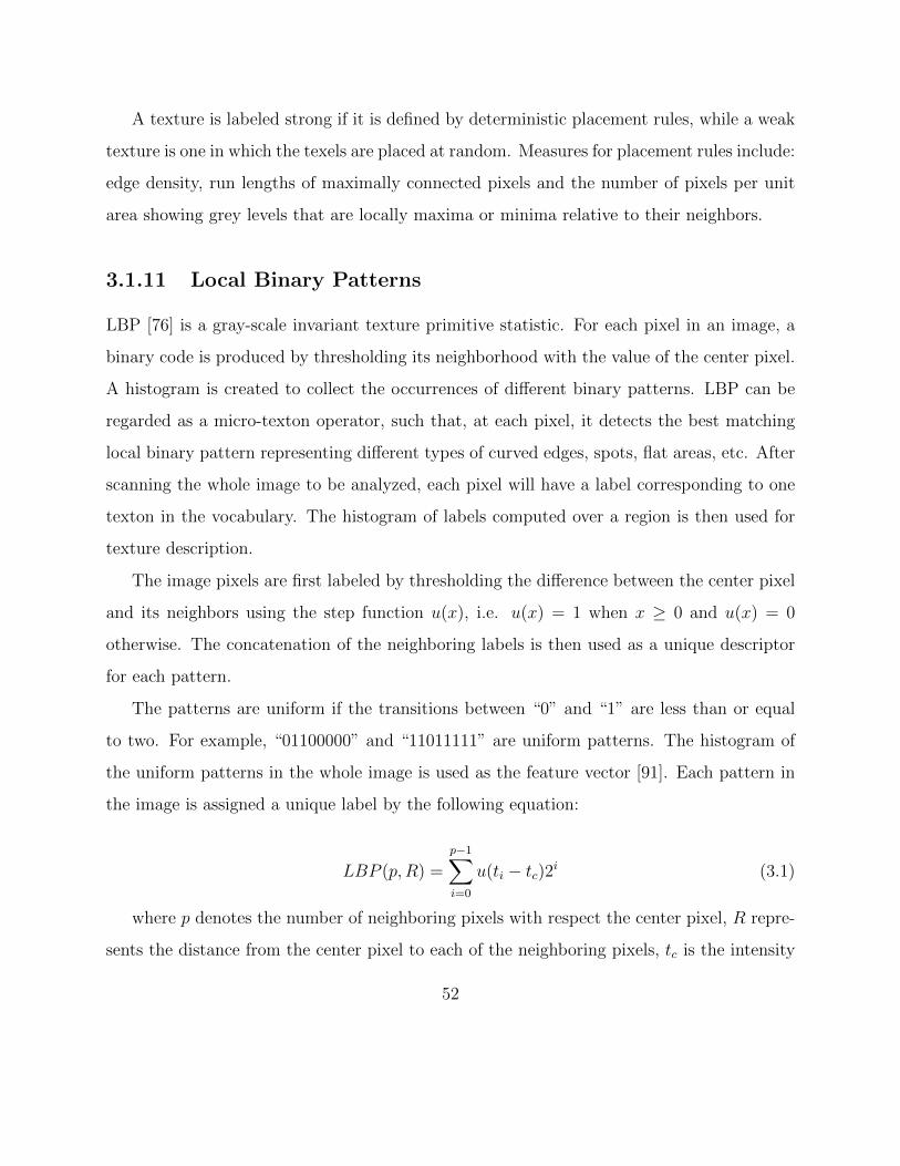
3.1.11 Local Binary Patterns
LBP [76] is a gray-scale invariant texture primitive statistic. For each pixel in an image, a
binary code is produced by thresholding its neighborhood with the value of the center pixel.
A histogram is created to collect the occurrences of different binary patterns. LBP can be
regarded as a micro-texton operator, such that, at each pixel, it detects the best matching
local binary pattern representing different types of curved edges, spots, flat areas, etc. After
scanning the whole image to be analyzed, each pixel will have a label corresponding to one
texton in the vocabulary. The histogram of labels computed over a region is then used for
texture description.
The image pixels are first labeled by thresholding the difference between the center pixel
and its neighbors using the step function u(x), i.e. u(x) = 1 when x ≥ 0 and u(x) = 0
otherwise. The concatenation of the neighboring labels is then used as a unique descriptor
for each pattern.
The patterns are uniform if the transitions between “0” and “1” are less than or equal
to two. For example, “01100000” and “11011111” are uniform patterns. The histogram of
the uniform patterns in the whole image is used as the feature vector [91]. Each pattern in
the image is assigned a unique label by the following equation:
LBP (p,R) =
p−1∑i=0
u(ti − tc)2i (3.1)
where p denotes the number of neighboring pixels with respect the center pixel, R repre-
sents the distance from the center pixel to each of the neighboring pixels, tc is the intensity
52

Figure 3.1: Local Binary Patterns
of the center pixel, ti is the intensity of the neighbor i and u(x) is the step function.
From Figure 3.1, it is shown an example of LBP, where p = 8 and R = 1: (a) the
original 3 × 3 neighborhood, where tc = 3 and ti = 2, 5, 4, 1, 1, 7, 4, 3, i = 0, . . . , 7; (c)
LBP weights; (d) the values in the thresholded neighborhood (b) are multiplied by the LBP
weights,u(ti − 3)2i, (c), given the corresponding pixels. The elements are then summed to
form the value of this textured unit, LBP (8, 1) =∑7
i=0 u(ti−3)2i = 2+4+32+64+128 = 230.
3.1.12 Advanced Local Binary Patterns with Rotation Invariance
Conventional LBP only considers the uniform patterns in the images. It discards important
pattern information for images whose dominant patterns are no uniform patterns. ALBPRI
[77] proposes a new rotation invariant texture classification method by extending the conven-
tional LBP approach to reflect the dominant pattern information contained in the texture
images and capturing the spatial distribution information of dominant patterns.
To formally define the “uniform” patterns, it is introduced a uniformity measure U(pattern),
which corresponds to the number of transitions, bitwise 0/1 changes in the “pattern”. For
example, patterns “00000000” and “11111111” have U value of 0, while patterns “01111111”
and “00000011” have a U value of 2 as there are exactly two 0/1 transitions in the pattern.
For ALBPRI, it is designated patterns that have U value of at most 2 as “uniform” and
proposed the following operator for rotation invariant texture description:
53

ALBPRI(p,R) =
∑p−1
i=0 u(ti − tc) if U(LBPp,R) ≤ 2
p+ 1 otherwise(3.2)
where
U(LBPp,R) = |u(tp−1 − tc)− u(t0 − tc)|+p−1∑i=1
|u(ti − tc)− u(ti−1 − tc)|
By definition, exactly p+ 1 uniform binary patterns can occur in a circularly symmetric
neighbor set of p pixels. Equation 3.2 assigns a unique label to each of them corresponding
to the number of “1” bits in the pattern (0→ p) while the nonuniform patterns are grouped
under the label (p+ 1) [91].
The final texture feature employed in texture analysis is the histogram of the operator
outputs, i.e. pattern labels, accumulated over a texture sample. The reason why the his-
togram of uniform pattern provides better discrimination in comparison to the histogram of
all individual patterns comes down to differences in their statistical properties. The relative
proportion of nonuniform patterns of all pattern accumulated into a histogram is so small
that their probabilities cannot be estimated reliably.
The LBP and LBPRI methods are widely used because they have the highest performance
of texture classification of the Columbia Utrecht Reflectance and Texture Database (CUReT)
[92], which is the most common and difficult benchmark used to test texture recognition
algorithms [76], [77], [93].
CUReT has the largest number of texture classes; it contains 61 different real-world
textures, each texture class under more than 200 different viewing directions. Therefore, it
is very difficult to classify such large number of textures because it can have small inter-class
distances in the feature space. This database actually is used to test how precise the features
of each approach can describe the texture images.
On the other hand, texture recognition has been also studied for manufacturing processes.
Surface roughness estimation of work pieces plays a key role for manufacturing industry.
54

Manufacturing systems focus to increase production, quality and to reduce costs and time so
as to produce a product. The surface roughness is a quality indicator of machined products
that are influenced by the cutting parameters. The texture classification methods focused on
the manufacturing industry are not very convenient because they require a highly controlled
environment; for example, a strict distance between the camera and the item to be tested,
always put the item in the same position, among others [94], [95], [96].
Despite the important advances in the recognition of textures, very little has been done
to develop algorithms focused on autonomous navigation of robots in outdoor terrain. For
the purposes of autonomous navigation of robots it is convenient to use the best method to
classify this kind of textures.
3.2 Appearance-Based Vision
ABM is a method employed mainly for object [97], [98] and face recognition [78]. The ABM
method gets the principal components of image distribution, namely, the eigenvectors of the
covariance matrix of the object images set [99]. The ordered eigenvectors fashion the features
accounting and charactering the variation among the different images.
The ABM has the advantage of reducing the dimensionality of high dimensional data
with a minimal loss of precision. This is suitable for processing high resolution images at
low computational cost.
Furthermore, both object and face recognition is different to texture recognition because,
for object and face recognition, it is not necessary to have high-detail data. As for texture
features, it is required to obtain their features at high-detail level. Specialized methods of
texture recognition found in the state of the art are very efficient, but its computational cost
is high, which can be a disadvantage.
However, as shown in the following chapters, for the purpose of velocity updating under
the proposed approach, there is no need to make an analysis with a high level of detail for
55

the classification of textures. It is sufficient to classify the textures only on their appearance.
In a similar way as humans do, in the following chapters it is analyzed this statement.
The use of ABM for object recognition involves the next list of operators and operations:
1. Let I1, . . . , IN ⊂ Rn×m the set of training texture images, where n and m are the
number of rows and columns, respectively, of the images and N is the number of
training images,
2. each training image is stacked and placed into the set of vectors φ1, . . . , φN ⊂ Rn·m,
3. all the vectors are normalized by φi = φi/‖φi‖, and placed into the set φ1, . . . , φN ⊂
Rn·m×N ,
4. the average vector C = 1N
∑Ni=1 φi is computed,
5. the matrix Φ = [φ1 −C, . . . , φN −C] is calculated,
6. the covariance matrix Ω = ΦΦT is computed,
7. the eigenvalues and eigenvectors of the covariance matrix are calculated as follows:
(a) the covariance matrix is transposed ΩT = ΦTΦ,
(b) the eigenvalues and eigenvectors are computed using the equation ΩTvi = λivi,
where λi is the ith eigenvalue and vi is the ith eigenvector,
(c) the eigenvectors are decreasing ordered according to their eigenvalues and placed
as columns of the matrix Λ = [v1, . . . ,vN ],
8. The eigenspace Ψ = ΦΛ is computed,
9. The eigenspace where each training image Ii is projected into γi = ΨT (φi − C), i =
1, . . . , N .
56

For texture classification, it is trained a Supervised Neural Network (SNN) using the set
of hand-labeled pairs (γ1, class), . . . , (γN , class), where γi is each of the training images
projections to the eigenspace and class is the corresponding texture class number. After
training, the SNN classifies the textures to be recognized by assigning a number of texture
class that most resembles. Following ABM the test texture image It is stacked and normalized
into ϕt, then projected to ωt = ΨT (ϕt −C) into the eigenspace Ψ; then the SNN compares
the with the classes of training textures, and the SNN output number indicates the class
number of the texture.
It is important to remark that the calculation of eigenvalues and eigenvectors is compu-
tationally very expensive because of the covariance matrix size. For instance, if images
would have a resolution of 480 × 640 pixels, then the covariance matrix size would be
307200 × 307200. Therefore, eigenvectors would be 307200-elements vectors so does the
projections of images to the eigenspace.
However, the size of the covariance matrix is significantly reduced, and therefore also the
computational costs, by a linear algebra theorem presented in [78], which states that the
eigenvalues of Ω = ΦΦT and ΩT = ΦTΦ are the same. Therefore, the eigenvectors of Ω
and ΩT are the same; thus, the covariance matrix size is N ×N .
Hence, the dimension of eigenvectors is N ; therefore the size of Λ is N×N . So, the images
projections to the eigenspace are vectors of dimension N . Therefore, the input dimension of
the data that feeds the SNN for recognition is N . Hence, it is concluded that the dimension
of vectors is a function of training set size; independently of the images’ resolution.
The broad ABM usage in computer vision has introduced the term Appearance-Based
Vision (ABV) [31], which is used in the rest of this thesis.
57

3.3 Experiments
To compare the texture recognition performance of LBP, ALBPRI and ABV, experiments
were performed, similar as were carried out in [76] and [77]. There were selected 20 classes
of textures from CUReT, with 30 training images per texture class with a view angle less
than 60 degrees, see Table 9 of Appendix A. The images for the training, and test, set were
selected by taking every alternate image and computing the average accuracy.
For texture classification using the ABV approach, it was employed a SNN. The SNN has
two layers, the first layer has 600 neurons and the second layer has 20 neurons. The activation
functions are hyperbolic tangent and sigmoid in the first and second layers, respectively. The
SNN was trained with the feed-forward backpropagation algorithm [100]. The experiments
were implemented using the image processing and neural network Matlab’s toolboxes.
With LBP and ALBPRI the histograms modeled each texture and in classification each
sample from the test set was assigned to the class of the closest model histogram. In both
LBP and ALBPRI, the number of neighboring pixels with respect the center pixel is p = 8
and the distance from the center pixel to each of the neighboring pixels is R = 1. In the
classification phase, it was evaluated the dissimilarity of sample and model histograms as a
test of goodness-of-fit, which is measured with a nonparametric statistical test. By using a
nonparametric test, it was avoided making any, possibly erroneous, assumptions about the
feature distributions.
For comparing the histograms in LBP and ALBPRI, the log-likelihood statistic L(S,M) =∑Bb=1 Sb logMb was employed, where B is the number of bins, Sb and Mb correspond to the
sample and model probabilities at bin b, respectively. Table 3.1 shows a performance com-
parative between related works and our approach for texture recognition using CUReT image
database.
The texture recognition results of Table 3.1 show that ABV method performance is not
as good as LBP and ALBPRI. A high-detail texture classification with ABV is difficult
58
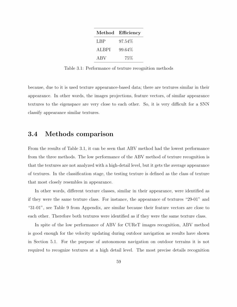
Method Efficiency
LBP 97.54%
ALBPI 99.64%
ABV 75%
Table 3.1: Performance of texture recognition methods
because, due to it is used texture appearance-based data; there are textures similar in their
appearance. In other words, the images projections, feature vectors, of similar appearance
textures to the eigenspace are very close to each other. So, it is very difficult for a SNN
classify appearance similar textures.
3.4 Methods comparison
From the results of Table 3.1, it can be seen that ABV method had the lowest performance
from the three methods. The low performance of the ABV method of texture recognition is
that the textures are not analyzed with a high-detail level, but it gets the average appearance
of textures. In the classification stage, the testing texture is defined as the class of texture
that most closely resembles in appearance.
In other words, different texture classes, similar in their appearance, were identified as
if they were the same texture class. For instance, the appearance of textures “29-01” and
“31-01”, see Table 9 from Appendix, are similar because their feature vectors are close to
each other. Therefore both textures were identified as if they were the same texture class.
In spite of the low performance of ABV for CUReT images recognition, ABV method
is good enough for the velocity updating during outdoor navigation as results have shown
in Section 5.1. For the purpose of autonomous navigation on outdoor terrains it is not
required to recognize textures at a high detail level. The most precise details recognition
59

methods are not adequate, because they fail to support robot navigation. LBP and ALBPRI
methods recognize patterns with lines, dots or borders, but fails for recognizing different
depicted appearances. For detailed recognition, ABM is not so exhaustive but provides the
enough capabilities for the recognition of terrain average appearance that it is the recognition
requisite for outdoor navigation.
For velocity updating, here is proposed to imitate the humans’ perception for texture
recognition, in order to strength the robot navigation abilities. Humans classify textures
according to past experience; when a human finds a new texture, he employs his experience
to determine to which texture class the new texture is more appearance similar. When
humans drive vehicles, they do not inspect the terrain textures with a magnifying glass nor
take a look at a small distance to account details of particular lines, dots or borders; they
just estimate the texture roughness basing on previous pattern recognition experience while
driving [1].
To imitate the human experience during texture classification for navigation, it is clever
to pay attention in convenient methods for recognizing the surface average appearance, such
that not lost in unnecessary details for the outdoors navigation purpose.
Moreover, frequently the recognition of surfaces’ details is computationally high-cost
and it should be avoided for autonomous navigation. Hence, there were implemented the
algorithms of LBP and ALBPRI methods in order to compute their execution time alongside
the ABV algorithms. The microprocessor employed for the algorithms’ testing is a Centrino
Core 2 Duo at 2 GHz and 1.99 Gb RAM.
It was measured the time the processor takes to run the algorithms of the ABV, LBP and
ALBPRI methods, to process and classify a 480×640 pixel image in grayscale. It was found
that the processor takes 0.13 seconds with ABV, 3.13 seconds with LBP and 8.62 seconds
with ALBPRI. Therefore, it can easily be concluded that LBP and ALBPRI methods are
computationally expensive, while the ABV method is cheaper than LBP and ALBPRI.
Chapter 5 shows that ABV advantages LBP and ALBPRI for outdoor navigation of
60

robots; thus, the ABV method is good enough for the velocity updating during outdoor
navigation.
Next chapter presents the velocity updating approach; by using fuzzy logic the human
process for identifying the terrain roughness can be modeled in such a way to be used by
the robot to mimic this human ability. It is shown that what is needed is to estimate the
roughness level of textures instead of to know if the textures are correctly classified.
The texture roughness is a fuzzy concept, where it is assumed that textures with similar
appearance have similar level of roughness. With the help of an expert human driver and
following his criteria, the textures are labeled with a roughness value and then ordered
depending on their roughness value. As well as the expert driver establishes the terrain
roughness-velocity relationship through the inference system.
An important feature to take care for both texture modeling and recognition is illumina-
tion, because ABV is light sensitive. Therefore, the better illumination is the better texture
model and recognition is. Changes in illumination should be avoided; bright and uniform
lighting during navigation is required to guaranty consistent texture recognition. The pres-
ence of shadows, which treatment is a hard task to pattern recognition [101] is out of the
scope of this work.
In summary, this chapter presents the state of the art methods for texture recognition. It
was found that LBP and ALBPRI methods have the highest performance for texture classi-
fication. ABV method was tested for classification of textures, which had poor performance
compared to methods LBP and ALBPRI. However, it is claimed that for autonomous nav-
igation purposes the ABV method is more suitable for texture recognition. This statement
is discussed in Chapter 5, although it is necessary to go through Chapter 4 to understand
how to estimate the velocity of the robot, taking into account the roughness of the terrain.
61

62

Chapter 4
Velocity Updating
For the purpose of autonomous navigation on rough terrains the detailed recognition of
textures is not a requisite. As is shown below, the high precision methods for the recognition
of details are not the adequate, because they fail for supporting robots navigation, strongly
some times. In addition, the detailed recognition of surfaces is computationally expensive,
but a low consume of resources is much recommended for the autonomous navigation [75].
Here is proposed to imitate the human perception by employing a neuro-fuzzy approach
for velocity updating. In this chapter it is explained how a neuro-fuzzy approach can be a
useful tool for the velocity updating purpose. Hence, to imitate the human experience for
terrain recognition and the corresponding velocity adjustments when driving, the choice of
an adequate method for recognizing the surface average appearance, without lost in unnec-
essary terrain details, is clever for outdoors navigation. The ABV method, having a low of
detailed texture recognition efficacy, see Table 3.1, is applied to recognize terrains’ average
appearance; ABV effectively support the velocity updating throughout outdoor navigation
as is shown in Section 5.1.
Artificial Neural Networks (ANN) are an automatic processing paradigm inspired by the
animals nervious systems, implemented for training artificial learning-based systems. NN
63

is a system connecting neurons that work together to produce emerging behaviors. The
connections are weighted, succsessively updated and trained in order to achieve the desired
behaviors. The NN are non-model systems, and are organized in a way to simulate the cells
functioning of human neural system -or one of the diverse alive beings. ANN learn from the
underlying relationships of data and have self -learning and -tuning capabilities, without the
need of previous knowledge about data relationship.
The Fuzzy Logic set the modeling of abstract heuristics provided from human experts.
However, the fuzzy logic rules lacks of self-tuning mechanisms regarding data relationships,
so it is especially difficult to decide the membership function parameters. However, Fuzzy
Logic allows incorporating human experience in the form of linguistic rules. Thus, the
ANN patterns recognition complements the Fuzzy Logic modeling of human driving into the
artificial vision for the velocity control of outdoor navigation.
The robot velocity adaptation obeys fuzzy logic rules which are designed accordingly to
a roughness-velocity relationship; the prior roughness grading is based on a ANN textures
classification. The robot’s navigation system will adapt its velocity according to the terrain’s
roughness, and will also indicate if the robot is able to climb certain slopes or it should move
around them.
For this thesis, it is considered the following:
• It is employed a wheeled-robot,
• the terrains’ irregularities are slopes:
– if the slope inclination is less than or equal to 15 degrees, then the robot can pass
on the slope;
– Otherwise, the irregularity is defined as an obstacle and the robot must move
around it.
• Neither illumination intensity nor illumination angle vary, i.e. it is assumed that the
64

terrains are uniformly illuminated.
4.1 Neural networks for roughness recognition
ANN are a knowledge system and automatic processing paradigm inspired by the animals
nervious systems. It is a system with connections between neurons in a network that work
together so as to produce a stimulus. Normally, the ANN has a defined number of elements
or neurons connected between them. The connections are an array between neurons and
their nature is determined by the network’s structure. The connections weights are set or
trained in order to achieve the behavior desired. ANN can be classified by their structure or
learning algorithms [100]. ANN are divided in two kinds: unidirectional ANN and recurrent
ANN [102].
In a unidirectional ANN, the neurons are grouped in layers. The signals flow from the
input layer to the output layer; the neurons are connected from a layer to the next layer,
but not in the same layer. Multilayer perceptron is an example of a ANN. Most of the
unidirectional ANN do a static mapping between the input space and the output space.
In recurrent ANN’s the outputs from some neurons feedback themselves. Thus, signals
flows frontward and backward. Hopfield network or Elman network are two examples of
recurrent ANN. Recurrent ANN have dynamic memory: their outputs show the actual inputs,
besides the previous inputs and outputs [103].
ANN are trained, mainly, with two kinds of learning algorithms: supervised and unsu-
pervised learning algorithms. Besides, there is a third kind, reinforcement learning, that can
be considered as a special supervised learning algorithm [104].
The supervised learning algorithm sets the strength or weight connections between neu-
rons according to the difference between the desired output values and the current output
values. Thus, supervised learning needs a teacher or a supervisor in order to show the desired
output values. Some supervised learning algorithms are the delta rule or backpropagation
65

algorithm [105].
Unsupervised learning algorithms do not need to know the desired output values. During
training, only the input patterns are presented to the ANN that, automatically, adapts the
neurons weight connections so as to put the input patterns into groups of similar features.
Some unsupervised learning algorithms are the Kohonen algorithm or competitive learning
algorithm [106].
During outdoors navigation, human drivers estimate the convenient vehicle velocity by
regarding their previous experience when driving on similar terrain textures. In other words,
human drivers estimate how rough, in average, the terrain is, instead if specific texture
details are recognized.
Human drivers that navigate on uneven terrains do not need to learn, or to know, about
specific details but on the textures average appearance. Hence, for texture classification it
is necessary the help of an expert driver to order the textures and to establish the texture-
class relationship. Thus, a supervised neural network is suitable for the current purpose.
The following sections show and explain the architectures of the ANN employed for texture
classification, roughness and velocity estimation.
4.2 Fuzzy logic for roughness estimation
For the purpose of texture recognition, and then to estimate the roughness of outdoor ter-
rains, it can be employ the LBP and ALBPRI. The disadvantage with these methods is that
they only have two possible outcomes, false and true, i.e. they indicate whether textures
have been identified or not. For velocity updating it can be too restrictive to use such classi-
fication methods. Moreover, what matters is to determine the roughness degree of textures.
By using only an ANN for texture classification it may cause that the robot takes wrong
decisions if a new class of texture is found.
Here is claimed that it is not necessary identify textures at a high-detail level for velocity
66

updating. For instance, when humans are walking, they do not inspect the textures with a
magnifying glass nor take a look at a small distance, they just estimate the roughness of the
new texture [1]; then they decide how fast they can walk without sliding. Usually human
beings do not need precise, numerical information to make a decision, but they are able to
perform adaptive actions, because there is a fuzzy concept in human knowledge.
Fuzzy logic is known to be an organized method for dealing with imprecise knowledge. Us-
ing linguistic rules, the fuzzy logic system simulates human decision making to deal unclearly
expressed concepts, to deal with imprecise or imperfect data, and to improve knowledge
representation and uncertainty reasoning. Fuzzy logic offers a framework for representing
imprecise, uncertain knowledge [29], [107]. They make use of human knowledge in the form
of linguistic rules. The robot velocity adaptation obeys Fuzzy logic rules, which are designed
accordingly to a roughness-velocity relationship.
The current proposal mimics the humans’ experience for terrain recognition with Fuzzy
logic [24], [28]. With Fuzzy logic, an expert human driver classifies and arranges represen-
tative data of specific environments, and according to the arranged data, sets the proper
velocity the robot can navigate safely.
By using Fuzzy logic the human perception sense is imitated to identify the robot’s
environment. A Fuzzy logic approach establishes ”how rough” the textures are by meta-
classifying them in roughness fuzzy sets. Thus, for autonomous navigation, it is advisable
to estimate the terrains’ roughness instead of whether the textures are recognized or not.
It is important to point that for textures and irregularities modeling, the most represen-
tative ones must be chosen depending on the kind of terrain to explore. For example, in a
wooded terrain the robot can find grass, leafs or branches, instead of sand or ice which can
be found on desert or glacier terrains respectively.
67

4.3 Neuro-Fuzzy approach
By mimicking the human perception for terrains’ roughness setting and velocity estimation
with Fuzzy logic approach, the robot will be able to move through terrains by adapting its
velocity according to the textures and soft irregularities it finds on its way, and deciding
whether it is able to climb a huge slope.
Fuzzy logic offers a framework for representing imprecise, uncertain knowledge. They
make use of human knowledge in the form of linguistic rules. But the disadvantages are
that fuzzy logic needs highly abstract heuristics, needs expert for rule discovery with data
relationships, especially, as it lacks of self-organizing and self-tuning mechanisms. This
results in difficulties to decide the parameters of membership functions.
Another drawback is the lack of a systematic procedure to transform expert knowledge
into the rule base. This results in many redundant rules in the rule base. On the other
hand, ANN are nonmodel systems that are organized in a way to simulate the cells of
human brain. They learn from the underlying relationships of data. ANN have self-learning
capability, self-tuning capability, without the need to know data relationship, and can be
used to model various systems. Therefore, fuzzy logic and ANN are combined to estimate
the robot’s velocity by regarding the terrains’ roughness.
The difference between conventional fuzzy logic and neuro-fuzzy methods, this thesis
takes advantage, is that neuro-fuzzy methods need much less rules, while conventional fuzzy
logic needs a large number of rules. This simplifies the structure of the neuro-fuzzy model by
reducing the number of the hidden layer neuron, and reduces the computational time [108].
Thus, the proposed methodology is the following. A set of the most representative
textures of the navigation environment are modeled with the ABV method; a SNN is trained
with the set of the representative textures, principal components, for classification. The SNN
is trained with the texture-class relationship established by the human expert driver.
A Fuzzy Neural Network (FNN) is trained to determine the velocity regarding the texture
68

Figure 4.1: Block diagram of the proposed approach for velocity updating
classes as well as the inclination angle of slopes. The robot moves at the estimated velocity
and acquires new images of the terrain; the cycle repeats while the robot is moving, see
Figure 4.1.
In summary, the offline and online steps of the algorithms for velocity updating regarding
the terrains roughness are next described:
Roughness identification (off-line training)
1. Select representative images of the terrain textures, where the robot moves on.
2. Characterize the texture using the ABV method, which computes the principal com-
ponentes of the images.
3. Train the SNN with the texture-class relationship established by the human expert
driver.
4. Train the FNN to determine the velocity regarding the texture classes as well as the
inclination of slopes, according to the expert driver’s directives, make the fuzzy sets
and the inference IF-THEN rules system.
69

Figure 4.2: Slope detection employing two infrared sensors. The infrared rays extend until
them “touch” a terrain irregularity, thus, a virtual right triangle is drawn, where the rays
play the role of cathetus and the irregularity as hypotenuse. The angle is computed with
simple trigonometric operations
Velocity updating and robot’s moving (on-line steps)
5. Acquisition of terrain images with the robot’s camera.
6. The SNN classifies the texture, this data is forwarded to the FNN.
7. The FNN inputs are both, the texture class and the slope inclination angle (to deter-
mine if the robot can pass on the slope, or should move around it).
8. With the texture roughness meta-classification and slope inclination data, the FNN
updates the velocity. The robot’s mechanical control system adjust the velocity.
9. The cycle is repeated as the robot moves, and the velocity is cycle updated.
For irregularities detection, two infrared sensors are mounted on the robot. The sensors
are located in the frontal part of the robot. The first infrared sensor projects its ray parallel
to the robot’s motion; the second infrared projects its ray directly to the floor, in other
words, perpendicular to the first sensor. The inclination angle of irregularities is computed
by trigonometric operations. Figure 4.2 shows how the inclination angle of slopes is computed
by employing the infrared sensors data.
70

4.4 Fuzzy neural network architecture
The network proposed is a five-layer FNN. The FNN has two inputs x (texture class) and
y (slope inclination), and one output f (robot’s velocity). Figure 4.3 illustrates the cor-
responding FNN architecture where a first-order Sugeno fuzzy model is proposed, and the
nodes of the same layer have similar functions, as described next. Here it is denoted the
output of the ith node in layer l as Oi,l.
The textures are meta-classified into the roughness categories high (H), medium (M) and
low (L), see Figure 4.4.
The slope inclination is divided into the fuzzy sets: plain (Pl), slightly plain (SP), slightly
sloped (SS), moderato sloped (MS), high slope (HS) and very high (VH), see Figure 4.5.
The neuro-fuzzy output values are high velocity (HV), moderate velocity (MV), low
velocity (LV) and stop (ST), see Figure 4.6. The fuzzy-making procedure maps the crisp
input values to the linguistic fuzzy terms with membership values in [0, 1].
The rule base stores the rules governing the input-output relationship. Taking A, B, C
as variables of the respective predicates, the form of inference rules is:
IF Slope angle is A AND Texture roughness is B THEN Velocity is C.
The fuzzy logic inference rules are listed in Table 4.1. Below are explained each layer of
the FNN.
Layer 1: Every node i in this layer is an adaptive node with a node function:
O1,1 = µr(L) O1,4 = µs(Pl) O1,7 = µs(MS)
O1,2 = µr(L) O1,5 = µs(SP ) O1,8 = µs(HS)
O1,3 = µr(L) O1,6 = µs(SS) O1,9 = µs(V H)
where x (or y) is the input to nodes into a linguistic label L, M, H (or Pl, SP, SS,
MS, HS, VH); µr and µs are the roughness and slope membership functions, respectively.
Parameters in this layer are referred as premise parameters.
71

Figure 4.3: Fuzzy neural network architecture. The FNN has five layers, the first layer has
two inputs, the slope inclination and the texture class, the second layer sets the terms of
input membership variables, the third one sets the terms of the rule base, the fourth sets
the term of output membership variables, and in the fifth layer, the output is the robot’s
velocity
72

Figure 4.4: Texture roughness membership function
Figure 4.5: Slopes membership function
Figure 4.6: Velocity membership function
73

Rule No. Input Output
Slope angle Texture roughness Velocity
1 Pl L HV
2 Pl M HV
3 Pl H HV
4 SP L MV
5 SP M HV
6 SP H HV
7 SS L MV
8 SS M MV
9 SS H HV
10 MS L LV
11 MS M MV
12 MS H MV
13 HS L LV
14 HS M LV
15 HS H MV
16 VH L ST
17 VH M ST
18 VH H LV
Table 4.1: If-Then rules of the FNN’s inference system
74

Layer 2: Every node in this layer is a fixed node label Π, whose output is the product of
all the incoming signals, O2,i = ωi, i = 1, . . . , 18, where:
ω1 = µr(L)µs(Pl) ω7 = µr(L)µs(SS) ω13 = µr(L)µs(HS)
ω2 = µr(M)µs(Pl) ω8 = µr(M)µs(SS) ω14 = µr(M)µs(HS)
ω3 = µr(H)µs(Pl) ω9 = µr(H)µs(SS) ω15 = µr(H)µs(HS)
ω4 = µr(L)µs(SP ) ω10 = µr(L)µs(MS) ω16 = µr(L)µs(V H)
ω5 = µr(M)µs(SP ) ω11 = µr(M)µs(MS) ω17 = µr(M)µs(V H)
ω6 = µr(H)µs(SP ) ω12 = µr(H)µs(MS) ω18 = µr(H)µs(V H)
Each node output represents the firing strength of a rule. The T-norm operator employed
is the algebraic product.
Layer 3: Every node in this layer is a fixed node label N. The ith node calculates the
radio of the ith rule’s strength to the sum of all rules’ firing strengths:
O3,i = $i =ωi∑18j=1 ωj
, i = 1, . . . , 18.
The outputs of this layer are called normalized firing strengths.
Layer 4: Every node k in this layer is an adaptive node with a node function:
O4,k = ωk(pkx+ qky + rk), k = 1, . . . , 4.
Where pk, qk, rk : k = 1, . . . , 4 is the parameter set of this node. Parameters in this
layer are referred to as consequent parameters. Hence, the consequent parameters are:
ω1 = $1 +$2 +$3 +$5 +$6 +$9,
ω2 = $4 +$7 +$8 +$11 +$12 +$15,
ω3 = $10 +$13 +$14 +$15,
ω1 = $16 +$17.
75

Layer 5: The single node of this layer is a fixed node labeled Σ, which computes the
overall output as the summation of all the incoming signals (center of area defuzzification
method):
O5,1 =4∑
k=1
ωkfk.
The defuzzification procedure maps the fuzzy output from the inference mechanism to a
crisp signal. The formula for computing the robot velocity is v = Vmax ·VFNN , where Vmax is
the maximum allowable vehicle speed and VFNN is the FNN output, a value in the interval
[0, 1].
For FNN training it is applied the hybrid learning algorithm. It is observed that when
the values of the premise parameters are fixed, the overall output can be expressed as a
linear combination of the consequent parameters [29]. The hybrid learning algorithm, which
combines steepest descent and the least-square estimator for fast identification of parameters,
identifies these linear parameters by least-square method.
The output f in Figure 4.3 can be rewritten as:
f = ω1f1 + ω2f2 + ω3f3 + ω4f4,
f = ω1(p1x+ q1y + r1) + ω2(p2x+ q2y + r2) + ω3(p3x+ q3y + r3) + ω4(p4x+ q4y + r4).
Hence:
f = (ω1)p1 + (ω1y)q1 + (ω1)r1 + (ω2)p2 + (ω2y)q2 + (ω2)r2
+ (ω3)p3 + (ω3y)q3 + (ω3)r3 + (ω4)p4 + (ω4y)q4 + (ω4)r4
which is a linear in the consequent parameters pk, qk, rk : k = 1, . . . , 4.
So, the training data pairs are ordered to form the m × 12 matrix A, called the design
matrix, and the m× 1 output vector y , then it is obtained matrix equation:
Aθ = y
76

where θ is an 12 × 1 unknown vector whose elements are parameters pk, qk, rk : k =
1, . . . , 4. This is a standard linear least-squares problem, and the best solution for θ, which
minimizes ‖Aθ − y‖2, is the least-squares estimator θ∗:
θ∗ = (ATA)−1ATy,
where (ATA)−1AT is the pseudoinverse of A if ATA is nonsingular. It can be also
employed the recursive least-squares estimator formula to calculate θ∗. Specifically, let the
ith row vector of design matrix A be aTi and the ith element of y be yTi ; then θ can be
calculated iteratively as follows:
θi+1 = θi + Pi+1ai+1(yTi+1 − aT
i+1θi)
Pi+1 = Pi −Piai+1a
Ti+1Pi
1+aTi+1Piai+1
.
The initial conditions needed are θ0 = 0 and P0 = γI, where γ is a positive large number
and I is the identity matrix.
In summary, this Chapter presents the conditions of the terrains on which this work
focuses. It is proposed a neuro-fuzzy approach to estimate the velocity of the robot as a
function of the characteristics of the terrains. It is proposed that the velocity updating is
performed by mimicking the human vehicle driving as well the estimation of terrain rough-
ness. Humans estimate the roughness of the terrains, based on their experience and without
complex mathematical calculations. Hence, the neuro-fuzzy approach is proposed to mimic
the behavior of human beings to update the velocity of vehicles in the navigation in outdoor
terrains with different classes of textures and irregularities.
The FNN has five layers, the first layer inputs are the slope inclination and the texture
class, the second layer sets the terms of input membership variables, the third one sets the
terms of the rule base, the fourth sets the term of output membership variables, and in
the fifth layer, the output is the robot’s velocity. The starting parameters values for FNN
training are provided by human expert drivers. When the robot finds a slope steeper than the
77

allowed threshold, it stops, and evaluates which movement to make, whose decision concerns
to path planning. The gradient method [33] is integrated to present proposal, as addressed
in Chapter 6.
78

Chapter 5
Experiments and Simulations for
Velocity Updating
This chapter presents two set of experiments and their results employing the neuro-fuzzy
approach. In the first set of experiments, there were recorded the estimated velocities using
the LBP, ALBPRI and ABV methods, and a method based on discrete Fourier transform,
for the texture recognition of the terrains. The textures where the robot is tested are ground,
grass and paving stone. The results indicate that the ABV method is best suited for velocity
updating, for navigation on outdoor terrains. It is given a brief description of the robotic
platform used for experiments.
The second set of experiments consists of simulating the velocity updating of a car. For
these experiments there was placed a video camera on a car, with a similar perspective to the
driver, which recorded the road with different classes of textures when the car was in motion.
The velocity estimation was made using images of the videotaped roads. The videotaped
textures were loose stones, ground with grass, ground, concrete and asphalt. It is shown
that the proposed approach is computationally inexpensive, which suggests the feasibility of
being implemented in a real vehicle.
79

Figure 5.1: Wheeled-robot employed for testing
5.1 Terrain recognition supporting navigation
For the autonomous navigation experiments a wheeled-robot from Bioloid transformer kit
is used [109]. Bioloid is an all-around robot kit that can be assembled in any way the user
wants. It is similar to a block toy, but whereas the user of an ordinary block toys is only
free to set the physical appearance of the toy, the user of a Bioloid can not only manipulate
the physical appearance but also set certain behavior patterns.
The robot uses a processing unit, four servomotors for power transmission to the wheels,
two infrared sensors located in the robot front, and a wireless camera on top-front of the
robot. It is easy to see in Figure 5.1 where all these devices are located on the robot. For
testing, it has been employed a wheeled-robot. The robot dimensions are 9.5 cm width per
15 cm length.
80

In this platform it is used a personal computer (PC) and the processor of the robot,
to form a master-slave architecture, wirelessly communicated. On the PC are implemented
and executed the path planning and velocity estimation algorithms. The robot, on one
hand, reports to the PC the sensors readings and wirelessly transmits the images captured
by the camera. On the other hand, the robot performs the movements in accordance with
instructions that the PC communicates it.
For these experiments, the training images texture images from the terrain shown in
Figure 1.1. The garden ground texture is covered by a thin coat of dust and dispersed little
rocks; the grass is about 2 cm height and dry; the paving stone contains leafs, tree branches
with a thin dust cover. In the training phase, there were used 30 images per texture class
and there were performed eight runs on the mentioned textures.
It is important to mention that the terrain where the tests were conducted does not
contain obstacles, as it has not been implemented any path planning algorithm. Thus, the
robot only performs straight line trajectories. What matters in these set of experiments is to
compare the performance of texture recognition methods for adjusting velocity of the robot
that moves in outdoor terrains, under the neuro-fuzzy approach proposed.
While navigating, images of terrain’s textures are acquired with the camera mounted on
it, then the robot sends the images to the computing unit to classify the terrain’s textures,
then it receives the instruction to update its velocity considering the current terrain fea-
tures, hence the robot navigates as fast and safe as possible. As quick as terrain roughness
significant change is detected, the robot receives the instruction for velocity updating.
For the detection and measurement of slopes inclination, an infrared sensor located in
the frontal part of the robot does parallel ray projection to the robot’s motion; the other
sensor projects its ray directly to the floor perpendicular to the first sensor. Figure 4.2 shows
the infrared rays extended until they “touch” a terrain irregularity, a virtual right triangle is
drawn with the rays as the cathetus and the terrain line as the hypotenuse, see Figure 4.2.
The slope angle of irregularities is computed by trigonometric operations. Remember that
81

the maximum angle of inclination that is allowed to pass on a slope is 15 degrees.
For comparison purposes the LBP and ALBPRI methods with the best performance on
detailed recognition are tested by using outdoors images for training. The terrain textures are
respectively modeled with ABV, LBP, ALBPRI methods, as well as with the discrete Fourier
transform for cast surface recognition (FCS) [71]. The FCS method is a two-dimensional
Fourier transform deserved to assess the cast surface quality, which it has showed high
performance in such application.
The log-likelihood statistic L(S,M) =∑B
b=1 Sb logMb was employed as the classifying
method for LBP and ALBPRI methods, where B is the number of bins, Sb and Mb correspond
to the sample and model probabilities at bin b, respectively. For ABV method, it was used a
two-hidden layer SNN for texture classification; the first layer has 90 neurons and the second
layer has three neurons. The activation functions are hyperbolic tangent and sigmoid in the
first and second layers, respectively. With the FCS method it was employed a SNN as a
classifier, trained with the backpropagation rule [100].
The expected behavior is that the wheeled-robot moves faster in paving stone, in second
place on ground and third place on grass. That is, it is defined the paving stone as a high
roughness texture, the grass as a medium roughness texture and grass as a low roughness
texture.
It can be easily deduced why it is established this roughness order to these textures. The
paving stone is a high-traction texture, which allows a vehicle to stop quickly to sudden
braking when the vehicle is moving at high speeds, i.e. the vehicle suffers minimal slippage
such that it does not compromise its integrity. Ground is less rough than paving stone but
has greater traction than grass. The ground texture has on its surface a thin layer of dust,
making the vehicles susceptible to slide more easily than on paving stone. For the grass,
the texture is defined as low-traction favoring wheel slippage due to its soft consistency.
Velocities for navigation on the outdoor textures in Figure 1.1 are shown in Table 5.1.
From Table 5.1, LBP and FCS methods strongly failed because they do not follow the
82

Method/Texture Grass Ground Paving Stone
ABV 2.64 5.42 6.86
ALBPRI 4.28 5.81 7.02
LBP 7.02 7.31 7.71
FCS 2.58 0.65 1.30
Table 5.1: Velocities estimated under the neuro-fuzzy approach by employing the ABV,
ALBPRI, LBP and FCS methods for texture classification. The velocities are estimated in
meter per minute units
expected behavior. The method ALBPRI presents the expected behavior, although the
estimated velocity for grass is close to the estimated for ground. With the method ABV, it
meets the expected behavior. With lower velocity estimation made with the LBP method,
but with ABV the velocities assigned to each texture class can more easily distinguish.
On the recognition phase based on ALBPRI and LBP methods using images from a low
roughness wall (near to terrain in Figure 1.1) together with terrain images, occurred that
both ALBPRI and LBP failed to recognize the textures and misclassify all the images as
wall-texture; the wall images were interpreted by LBP and ALBPRI as noise instead of useful
data.
A likely explanation for this fail is that ALBPRI and LBP recognition are based on the
presence of borders, edges and dots that need to be detected to ensure these methods well
recognition performance. The wall images are uniformly plain and, perhaps, the required
graphical elements for these methods to perform well are not present, causing that LBP and
ALBPRI missed to recognize surfaces not clearly marked with lines, borders or dots. As a
consequence, the induced velocity updating is wrong during the terrain navigation.
Actually, humans at driving vehicles do not inspect the terrain textures with a magnifying
glass nor take a look at a small distance to account details of particular lines, dots or borders;
83
they just estimate the texture roughness basing on previous pattern recognition experiences
while driving [1].
On the other hand, the ABV method does properly recognize the outdoors terrain tex-
tures changes, and accordingly the robot’s velocity of navigation is updated. ABV method
advantages LBP and ALBPRI to recognize what can be called the average appearance in
the images of outdoors surfaces. In reported experiments the ABV method recognized well
the wall average appearance, as well as the average appearance of grass, ground or paved
-whereas LBP and ALBPRI stay away or fail.
Likely, recognition of the average appearance supports the robots navigation on out-
doors terrains. Actually, regarding the terrain average appearance is how humans drive the
wheeled vehicles. Car drivers update velocity by regarding the terrain average appearance,
i.e. velocity adjustments are according to the terrain texture average variations, which are
relevant to human drivers during navigation, and disregarding the irrelevant specific lines,
dots or borders.
In the FCS method the two-dimensional Fourier transform deserves to assess the cast
surface quality. This method shows high performance in classification by recognizing polished
surfaces like glass, steel or plastics, and such that images are very closely taken (9 cm). FCS
applied to Figure 1.1 terrain images failed hardly. All the obtained results were wrong;
the method missed to classify the terrain’s textures as low roughness textures, see Table
5.1. The plausible explanation is that this method works on polished texture that requires
high precision recognition. Furthermore, it also misses on rough surfaces like grass, ground,
soil or pave that not demand so high precision during textures recognizing -but an average
appearance recognition.
Hence, to imitate the human behavior of terrain recognition to adjust velocity during
driving, the choice of the right method for recognizing the surface appearance average, with-
out lost in unnecessary terrain details, is clever. Moreover, the surfaces details recognition
is computational expensive and waste of computing resources must be avoided through au-
84

tonomous navigation.
Based on the experiments, the ABV is the best pattern recognition method for supporting
the velocity updating of wheeled-robots navigation. ABV recognition algorithms successfully
classify terrain textures by regarding the average of the appearance. The high-detailed
recognition algorithms success in recognizing patterns depicted with lines, dots or borders,
but they fail for recognizing patterns where the average appearance is required. As human
driving experience shows, the assessment of the average appearance is needed for velocity
updating during navigation on outdoor terrains.
The more the terrain roughness is the more the vehicle’s velocity, as it is shown in the
results of these experiments; the velocity differences between navigating on ground and on
paving stone roads is fewer than between ground and grass roads. Results are consistent with
the expert driver recommendation, and, at a first glance, useful for real robotic displacement
on outdoors.
It is important to mention that the wireless camera captures 30 frames per second. For
our purpose, only one image is used from the 30 captured images, i.e., an image is processed
per second. That is because the maximum speed of the robot is 8.32 meters per minute and
at this velocity, the vehicle would have traveled 0.0046 meters in 1/30 seconds; from the
perspective of the camera the difference between the first and second images is negligible. In
addition, the robot does not always reach its maximum speed but it usually moves slower;
therefore, the robot travels are of short distances hence the surface images captured on these
condition are not truly different each other.
5.2 Simulations at real car velocities
The proposed method is not limited to be applied to small vehicles but can be extrapolated
to vehicles of different sizes, with particular characteristics which define the appropriate
rules of the vehicle operation. The algorithm is scalable to different vehicles by using as
85

parameters their particular features such as, weight, size, motor power, tires material, tire
tread, among others.
In this set of tests, terrain textures images are taken from video films with a camera
placed two meters above the floor on a truck’s roof, this camera films the road in front of
the vehicle, with a visual field similar to that of a person driving a real car, see Table 5.2.
The images are of outdoor terrains textures -most of them are real roads- such as ground,
ground with grass, concrete, asphalt and loose stones, on which the truck moves through.
These video images are employed to train the SNN and the FNN; the ABV method is used
to model the textures of both phases: training and recognition. The sampling time of tests
is one image per second.
Again, a human driver’s experience allows defining the classes of textures that can be
found in specific environments, e.g. in desert or mud environments, and then the right
speed a car can safely navigate is established. The textures classes are due by the SNN and
they are the FNN training input to identify roughness, therefore, via the inference rules the
corresponding velocity the vehicle can deploy on each terrain texture is assigned.
To implement the velocity updating algorithms in cars, it is important that the cars
have enough time to react to changes in roughness in the terrain while they are navigating.
Thus, it is important to take into account the computing capacity of the available hardware
to process the images captured by the video camera, in order to determine the maximum
velocity the car can reach. That is, the maximum velocity of the car must be set as a function
of the computing capacity of hardware. Car simulation tests are carried out with the vehicle
at a maximum speed of 60 km/hr.
It can be easily deduced why it is established this texture-velocity relationship to these
textures. The texture of asphalt is a material specially designed for the motion of vehicles.
Hence, for this kind of texture is expected the FNN calculates the maximum velocities. In
the texture of concrete, its use is similar to asphalt, but this texture is often more slippery
than asphalt. Therefore, it is expected that the estimated velocities for concrete are less
86

Texture Image
Loose stones
Ground with grass
Ground
Concrete
Asphalt
Table 5.2: Videotaped textures in outdoor terrains from the perspective of a driver in a car
87

than on asphalt.
The ground texture is more slippery than asphalt and concrete, because on the surface
of this texture there is a thin layer of dust, which facilitates the cars skid. Therefore, the
estimated velocity for ground must be less than on asphalt and concrete. As for the grass with
ground texture, due to the soft consistency of grass, it makes the cars slip easily. Therefore,
the estimated velocity for ground and grass must be less than the estimated for sole ground.
Finally, the lowest velocity should be estimated for loose stones, since stones do not allow
the wheels of the vehicles to make proper contact with the floor and thus, the vehicles skid
more easily.
Therefore, the expected behavior is that the velocities magnitudes are estimated, from
low to high, in the following order:
1. Loose stones, the smallest velocities are estimated for this texture class;
2. Ground with grass, the velocities estimated for this texture class are bigger than on
loose stones but smaller than on ground;
3. Ground, the velocities estimated for this texture class are bigger than on ground with
grass but smaller than on concrete;
4. Concrete, the velocities estimated for this texture class are bigger than on ground
stones but smaller than on asphalt;
5. Asphalt, the highest velocities are estimated for this texture class.
The videos last approximately 8 minutes; there were used 30 training images per texture
class, which were obtained from videos. Training images are images of the first 30 seconds
of each video; the testing images are obtained after the second 30 of each video. After the
second 30 of each video, it is extracted an image at every second in the videos for testing,
giving a total of 420 testing images. The results of this experiment are shown in Table 5.3.
88

Texture Velocity (km/hr)
Loose stones 10.56
Ground with grass 18.47
Ground 27
Concrete 43.79
Asphalt 48.91
Table 5.3: Velocity updating results by employing the texture classes shown in Table 5.2
A likely proportional roughness-velocity emerges at some extent: the estimated velocities
magnitude increase as the textures are rougher. However, this ratio can vary up to the
particular terrain conditions, e.g., being affected by the weather conditions.
Actually, the velocities of Table 5.3 are the average of the ones resulting in specific
experiments. The minimum and maximum velocities recorded for loose stones are 10.56
km/hr and 18.91 km/hr, respectively; the velocity difference is 8.35 km/hr implying an
acceleration of 2.32m/s2 -which is the 23.65% of gravity acceleration. A vehicle that moves
on the texture of loose stones must move slowly because the stones favor the vehicle skids
and, if the vehicle moves at high speeds it can suffer severe vibrations.
The velocities estimated for ground with grass are slightly higher. Mostly the velocity
remains at 18.11 km/hr. Ground with grass texture is less abrupt than loose stones. The
grass does not cover the entire surface but there are holes with ground, usually small, even
so a car can pass over them at low-speed motion while avoiding damage due to vibrations
in the vehicle. Even when the grass is a texture that favors slides, unlikely the loose stones,
the wheels surfaces of the car have grater contact with the ground, thus the risk of slip is
smaller, but higher than in the next textures.
For ground textures, the velocity estimation behavior is similar to that of ground with
grass; the velocity remains constant at 27.61 km/hr in almost the entire path. The surface of
89

ground texture is covered with dust and very small stones, and is almost flat, so the vehicle
can move fast without being affected by strong vibrations, even the small stones and dust
in the surface could make the car to slide.
Velocity for concrete texture remains constant at 44.44 km/hr in almost the entire path,
-with 8.35% and 4.95% of gravity acceleration. Finally, the velocities estimated for asphalt
remain without changes, 48.91 km/hr throughout the entire path. The textures of concrete,
paving city streets, and asphalt covering roads are very similar. These covering materials
create a uniform surface, without holes and slopes, avoiding car slides.
An additional aspect to consider concerns the vehicle’s computing capacities to process
texture images and update velocity in real time. Computing capacities support or restrict
the process efficiency, and need to be considered as is next explained.
5.3 Cycle time: vision processing and velocity updat-
ing
The acquired images have a resolution of 480 × 640 pixels and are converted to grayscale.
The microprocessor employed during the algorithms test is a Centrino Core 2 Duo at 2 GHz
and 1.99 Gb RAM. If the vehicle moves at 60 km/hr, the mentioned processor takes 0.3
seconds for both image processing and velocity estimation to update the vehicle velocity.
Actually, there are two aspects to be considered for efficient velocity control:
• determine the range of the camera to capture surface images and
• the sampling time given the progress of the vehicle.
Concerning the sampling time, the video system captures 30 frames per second. However,
as above mentioned, it is not necessary -even not possible- to process all the 30 images pic-
90

Figure 5.2: Car vision/recognition system. The camera must process the next 5-meter road
segment before the vehicle passes over. That is, when the vehicle moves the first 5-meter
stretch, the computer processes the image of the posterior 5-meter stretch. When the second
stretch processing is finished, the vehicle would have started to move in the second stretch.
This cycle is successively repeated
tured in a second because several will be very similar among them, with negligible differences
given the vehicle acceleration on the mentioned roads.
Considering the 0.3 seconds that takes to process roughness recognition and velocity
updating, and assuming that the maximum speed is around 60 km/hr, the vehicle will
advance 5 meters, as shown in Figure 5.2.
The sampling time is an aspect that should be defined considering the hardware com-
puting capacity and the maximum speed the vehicle can reach. If the vehicle moves at low
speed, e.g. 3 km/hr, and 30 frames per second are sampled, it will result that the captured
images are almost the same. Thus, it makes no sense to process the 30 images sampled at
every second but is enough to process just a few images. But if the vehicle moves at a higher
speed, e.g. 60 km/hr, as the vehicle travels more terrain in less time it is necessary to get
data from the surface more frequently, such that vehicle has enough time to react to changes
in roughness. The sampling time must be longer, hence the captured images processing is
intense, and it is mandatory to process the 30 frames captured per second.
91

Therefore, it is relevant to consider the computing capacity of available hardware to
set the maximum sampling time and thus the speed the vehicle can reach. It is desirable
to adjust the sampling time as a function of vehicle speed, but this is beyond the scope
of this article. It is important to observe that in order to test the algorithms of texture
recognition and velocity updating at real scenarios, no representative benchmarks, or data
sets, or specific procedures for evaluating and comparing different systems [1] are available.
In summary, in this chapter there were compared the performance of texture classification
methods LBP, ALBPRI, ABV and FCS, applied to velocity updating under the proposed
neurofuzzy approach. It was concluded that the ABV method is best suited to update the
velocity of the robot basing on the terrains’ features. ABV method classifies the terrain
textures by regarding the average of the appearance. LBP and ALBPRI methods success
in recognizing patterns depicted with lines, dots or borders, but they fail for recognizing
patterns where the average appearance is required.
Simulation was carried out adjusting speed of a car, using images of roads, which were
acquired from the videotapes of the road where the car moved. Simulation results show
that this approach can be scaled to large vehicles. The results indicate that given the low
computational cost of the neurofuzzy approach and depending on the computing capacity of
the hardware used, it can allow vehicles to reach high speeds.
92

Chapter 6
Odometry-Based Localization
Improvement
Autonomous navigation requires calculating the location of wheeled-robots. To compute
the wheeled-robots’ position the odometry-based methods are frequently used to calculate
distance between the current and target positions of the wheeled-robot; however, the draw-
back using these methods to learn the wheeled-robots’ precise position is due to the wheels’
slippage, which is a common circumstance during outdoor navigation. In other words, the
autonomous wheeled-robots that use odometry to compute their own location have the dis-
advantage of generating errors due to wheels’ slippage.
Most of the works, that employ odometry, are aided by landmarks or other devices to
improve the calculation of the robots’ location [22], [24], [110]. The drawback of these ap-
proaches is the high computing cost. The current proposal reduces the wheels’ slippage by
using the robot velocity updating regarding the terrains’ roughness [75]; hence, the right ve-
locity displacement prevents the wheeled-robots from slipping, which is a relevant advantage
for odometry-based robot localization methods, so common for this purpose.
The results of this chapter show the localization improvement of wheeled-robots by ap-
93
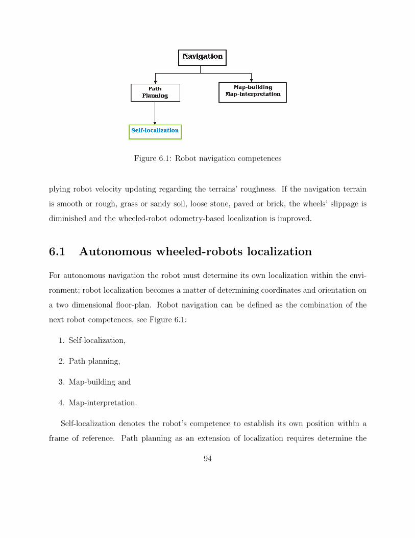
Figure 6.1: Robot navigation competences
plying robot velocity updating regarding the terrains’ roughness. If the navigation terrain
is smooth or rough, grass or sandy soil, loose stone, paved or brick, the wheels’ slippage is
diminished and the wheeled-robot odometry-based localization is improved.
6.1 Autonomous wheeled-robots localization
For autonomous navigation the robot must determine its own localization within the envi-
ronment; robot localization becomes a matter of determining coordinates and orientation on
a two dimensional floor-plan. Robot navigation can be defined as the combination of the
next robot competences, see Figure 6.1:
1. Self-localization,
2. Path planning,
3. Map-building and
4. Map-interpretation.
Self-localization denotes the robot’s competence to establish its own position within a
frame of reference. Path planning as an extension of localization requires determine the
94

robot’s current position as well as the goal location position, both within the same frame of
reference. Map denotes any one-to-one mapping of the world onto an internal representation.
Map-building covers any notation describing locations within the frame of reference. The
map charts explored territory within the frame of reference. Finally, to use a map, the ability
to interpret the map is needed.
For wheeled-robots, odometry is frequently used for self-localization [22]; but odometry
inevitably accumulates errors due to causes as the diameters of the wheels are not equal or
poor wheel alignment, wheel slippage, among others [23]. Wheel slippage is produced mainly
by [8], [30]:
• low-traction terrains,
• extremely fast rotation of the wheels,
• deformable terrain or steep slopes.
Most of the works on robotic autonomous navigation over outdoors have included limited
terrains’ features information in their proposals [5], [18], [20], [111]. One of the reasons is the
expensive computing cost for processing terrains’ roughness. The lack of terrains’ roughness
information makes difficult to compute a precise localization of autonomous robots as well
as to achieve the target position while the robot navigates over outdoor terrains.
Several works have managed to reduce the odometry errors by modeling errors from the
readings of the encoders coupled to the robot wheels to improve the robot self-localization.
Their results show reduction of odometry errors; but all these works are assisted by land-
marks [24], laser beams [25] and artificial vision [26], among other tools to identify the
terrains’ references [27]. This involves more information processing and, thus, increases the
computational cost.
The wheeled robot’s location control problem is a topic widely studied, due to the the-
oretical nature of the problem and its practical importance. Instead of building a control
95

problem where the robot requires a priory trajectory, in [35] formulates a velocity field track-
ing problem. Specifically, a velocity field is developed by the robot’s restricted trajectory,
and a differential controller is formulated in order to test the global asymptotic velocity
field. The kinetic controller developed is added inside the adaptive controller that foments
the global asymptotic tracking.
Wheeled robots have been employed for hazard environments such as the lunar surface.
Velocity estimation is important for lunar rovers because they navigate on rough terrain.
The wheel and terrain dynamic effects, like wheel slip, make difficult to real-time estimate
the vehicle’s velocity. Besides, it is difficult to observe the acceleration sensed data because
lunar rovers move at very low velocities. Song et al. [37] propose a kinematic-based method
for lunar rovers’ velocity estimation, using encoders and gyrometers. The kinematic model
is determined with the closed-velocity-chain theory. The velocity estimation is computed by
solving the vehicle’s kinematics.
In [8] is proposed a longitudinal wheel slip estimation-based model and immobility con-
ditions detection of autonomous mobile robots. It presents a new wheel model so as to
compute the dynamic forces of the rover. The rover’s external forces and velocity estimation
are obtained employing encoders, inertial measures and GPS. The experimental results show
that the technique detects immobility conditions while estimates the robot velocity during
a normal excursion.
Here is proposed that the robot adapts its velocity so it reaches the maximum velocity that
allows it to stop quickly enough without sliding, and moving slowly at low-traction surfaces
to avoid wheels’ slippage. Both wheels’ slippage and robot sliding, and consequently the
odometry errors, are reduced with velocity updating regarding the terrains’ features. Precise
location and target achievement can be improved this manner.
96

6.2 Odometry
Navigation as a challenging competence of mobile robots requires the competence to deter-
mine their own position in the environment. A well known way to calculate the location of
wheeled-robots is through odometry, by using readings of encoders coupled to the wheels
of the robot. The robot’s location is determined by calculating the robot’s traveled dis-
tance from initial to target position. However, odometry is susceptible to accumulate errors
during the robot course; the longer the trip is, the bigger the odometry error is. Mobile
wheeled-robots employ diverse techniques to reduce odometry errors in localization.
To overcome this difficulty, all mobile robot works are assisted by other devices, such as
electronic compasses [27], sonar sensors [4], GPS [112], among others. Thus, autonomous
robots’ proposals have focused on getting more information from the environment, but the
problem of reducing wheel slippage has not been fully addressed [30]. The works that use
odometry along with other devices to compute the location of the robots, report the error
rates with respect to their final location, i.e. how far the robots were located from the desired
position. Below are cited some related works on odometry-based localization methods.
Martinelli et al. [25] present a method allowing simultaneous robot localization and
odometry error estimation. The estimation of the systematic components is carried out
through an augmented Kalman filter, which estimates a state containing the robot config-
uration and the parameters characterizing the system component of the odometry error. It
uses encoder readings as inputs and the readings from a laser range finder as observations.
The filters are integrated in a coherent framework allowing autoing-calibrating the odometry
system while localizing during the robot navigation.
In [26], the robot odometry-based localization uses a memory of horizontal bearings
to landmarks. The method does not need internal representation of the robot’s position,
which is updated by alternating motion and sensor updates, and it does not depend on
distance measurements, which often are inaccurate when obtained by the size of far-distant
97

landmarks. The approach works on a buffer of observations and the history of the robot’s
odometry. Robot’s position is directly estimated by this data without alternating sensor and
motion updates.
O’Kane [113] presents a robot localization technique with linear and angular odometers,
whose configuration is composed from position and orientation, in a fully-known environment
by alternating rotations and forward translations. In the robot’s information space it is a
discrete-time planning problem. Localization by odometry is limited to simply-connected,
bounded polygonal symmetries environment.
In [114] the results of navigation of a mobile robot in outdoors shown position error rate
of 1% in 300 meters paths. In this work is used the visual odometry to estimate frame-to-
frame motion from stereo cameras and integrate the incremental motion with GPS. It uses
a bundle adjustment over multiple frames, which reduces the error while it is still operating
in real-time. The usage of stereo vision to estimate the motion provides more stability than
with a monocular camera. However, the computational cost of processing the real-time
stereo vision is of more computing and integration expensive as well [115].
Santana et al. [110] propose a localization system where the robot navigates in an
unknown environment, and the floor lines are used as landmarks and are identified. The
prediction phase using the extended Kalman filter is performed using the odometry model
of the robot. During the update phase, the proposal approach uses the parameters of the
lines detected by the Hough transform algorithm to correct the robot’s space.
Seraji and Werger [27] present several algorithms to calculate the location of a mobile
robot. The Weight average with local priority (WAL) and Peak-with-high-neighbors (PHN)
methods showed the best results in trajectories of 13 meters (measured in a straight line
between start and end points), with location error rates of 4% and 3.92% for PHN and WAL,
respectively. The approach combines data from both wheel odometry and the electronic
compass mounted on the robot. This scheme continuously decomposes all motion commands
into short straight-line segments. The compass is employed to orient the robot to the proper
98

direction at the beginning of each segment, and to correct for deviation from this heading
at the end of each segment. The straight-line distance traveled is computed with wheel
odometry, and the segment information is continuously accumulated to provide position
information. The location error is very similar to that obtained with our approach. But in
[27] an electronic compass to correct the underlying error of odometry is needed.
The mentioned works concentrated on reducing the underlaying odometric errors by
employing mathematical methods or using other devices to calculate the location of the robot;
but they need more computing power to process all the information they have acquired.
Actually, here proposed robot localization would be improved by combining velocity
updating with other localization methods, besides odometry, as those mentioned before. In
addition, the current proposal is easy to implement, computationally low-cost and does not
require sophisticated hardware, it just requires a video camera and two infrared sensors,
which is common equipment on wheeled-robots.
6.3 The navigation algorithm
Nowadays, beyond the detection and avoidance of obstacles, the velocity control of wheeled-
robots regarding the terrains’ features has not been attended exhaustively [4], [14], [30]; this
fact is a weakness for efficient navigation on outdoor terrains. Exploration robots in general
and particularly wheeled-robots need enough information about terrains’ features to ensure
efficient navigation. Moreover, to ensure precision on achieving the target, data of terrains’
roughness is an essential requisite.
The autonomous navigation of robots on outdoor terrains requires the concurrent opera-
tion of path planning and velocity estimation algorithms hence both harmonizing, see Figure
6.2.
99

Figure 6.2: Scheme integration of path planning and velocity estimation algorithms for
autonomous navigation
6.3.1 Path planning and velocity updating
The first step is to create a virtual map of the robot’s navigation space. The surface is
discretized by diving it into squares, where the amount of squares depends on the dimension
they occupy in real world, and the provided details of space model. The greater detail
the more computational resources are demanded for calculation of trajectories. The known
locations of obstacles, partial or complete, are recorded in the virtual map. It follows to
compute the optimal path between initial and goal locations with the gradient method.
Each time the virtual map is updated a new trajectory is calculated.
Then, the texture recognition algorithm is turned on to classify textures. The texture
classes alongside the slopes’ inclination are processed by the FNN to update the robot
velocity. Hence, the robot receives the instruction to move at the estimated velocity in the
prior determined trajectory. If during the travel the sensors detect an obstacle, or slopes with
inclination greater than 15 degrees, the robot stops and the velocity estimation algorithm is
turned off. The obstacle is registered, a new path to the goal location is recalculated and
100

the robot moves around the obstacle.
After that, the velocity estimation algorithm is turned on and the robot moves towards
the goal location in the new trajectory at the estimated velocity; otherwise, if the sensors do
not detect obstacles, the velocity is updated while the robot moves in the prior trajectory.
Note that the velocity estimation algorithm does not run all the time; it is turned off
when the robot finds an obstacle. At this circumstance, the camera captures images of the
obstacle instead of capturing the texture of the surface. If the velocity estimation algorithm
would not be turned off, the velocity would be estimated based on images of the obstacle’s
texture. Furthermore, the relevant in this case is that the robot overcomes the obstacle with
specific movements and not velocity changes.
The robot stops when it determines it has reached the goal location, by computing the
distance it has traveled from the initial location to its current location. The following list
summarizes the steps, see Figure 6.3:
1. Create a virtual map of robot space navigation, surface discretization,
2. Define the robot’s initial and goal locations,
3. Compute the path with the gradient method,
4. Texture recognition algorithm is turned on,
5. Velocity is estimated with surface data from textures classes and slopes,
6. Robot receives the order to advance along the path, at the estimated velocity,
7. Robot’s velocity is updated when a change in texture is recognized, or sensors detect
a slope on the surface, or both events occur,
8. If sensors detect an obstacle or slope inclination greater than 15 degrees, then the
robot stops and texture recognition algorithm is turned off; return to step 3; otherwise,
velocity is updated, and return to 7,
101

Figure 6.3: Flow diagram of the navigation algorithm, where the path planning and veloc-
ity updating algorithms are integrated to work harmonized for autonomous navigation on
outdoor terrains
9. The robot stops when it has reached the goal location or destination.
6.3.2 The gradient method
The path planning algorithms for mobile robots differ among depending on the robot appli-
cation: exploration of unknown territory [1], car navigation on roads [2], planet exploration
[116], indoor navigation [19], or if the environment is dynamic [111] or static [117] The al-
gorithms that use more data from environment are more accurate but more expensive and
difficult to implement too [23].
For the current purpose, a path planning algorithm that is suitable for an environment
102

that we assume is partially or totally unknown which is static and with obstacles of various
sizes, and computationally low-cost is picked. The robot must travel on the estimated path
by updating its velocity depending on the characteristics of the surface.
The path planning algorithm of gradient method [33] recalculates the paths in real time
every time it encounters an obstacle and it is suitable for static environments; this method
is the most convenient to support path planning in present proposal. The gradient method
uses a navigation function to generate a gradient field that represents the optimum path to
the destination point at each point of the workspace.
The gradient of the navigation function represents the direction of the path with the
lowest cost at each point in space. The method requires a discrete configuration of space
navigation in which the path cost function is sampled. A navigation function is calculated in
the local space of the robot, such that the gradient of the function represents the direction
of the path with the lowest cost at each point in space.
The optimum path to the destination point is calculated continuously. The concept of
optimal cost is derived from assigning costs to paths basing on their length and proximity to
obstacles, as well as any other criteria one may choose. The gradient method can lead the
path with the lowest cost in static and completely unknown environments, and it is efficient
for real time monitoring of movements of mobile robots, being equipped with laser beams.
Thus, the gradient method is described as follows. A path is represented by an ordered
set of points in the sample space P = p1, p2, . . . , where the set of points re contiguous
(either diagonally or rectilinearly), and no point repeats. The last point on the path must
be a goalset point, and no other point can be. A path that starts at point k is abbreviated
as Pk.
In general, the cost of a path is an arbitrary function of the (discretized) path, F (P ).
But such cost functions are difficult to deal with, and then it is made the assumption that
the path cost is separable into the sum of an intrinsic cost of being at a point, along with
an adjacency cost of moving from one point to the next: F (P ) =∑
i I(pi) +∑
iA(pi, pi+1).
103

Both I and A can be arbitrary functions. For typical situations, I represents the cost of
traversing through the given point, and is set according to the domain characteristics, e.g.,
a high cost will be assigned to being near an obstacle. Other possibilities are to have higher
costs or unknown regions, slippery regions, etc.
The path length is taken into account by assigning A to be proportional Euclidean dis-
tance the robot travels between the two points; then the sum of A gives a cost proportional
to the path length.
A navigation function N is the assignment of potential field value to every element of
the configuration space, such that the goalset is always downhill no matter where the robot
is in the space. Navigation functions, unlike potential field methods in general, have the
characteristic that it is impossible to get stuck in a local minimum, and no search is required
to determine direction to go arrive at the goalset.
The key idea behind the gradient method is to assign the navigation function at a point
to be the cost of the minimal cost path that starts at that point. Mathematically,
Nk = minPk
F (Pk),
where as before, the path Pk starts at point k. If the intrinsic costs are zero, then the
navigation function just represents the distance to the nearest goalset point. Traveling in
the direction of the gradient of N yields the fastest reduction of path cost, i.e. the minimum
distance to a goalset point. In the general case, traveling along the gradient is a minimum
cost path to the goalset.
Computing the values of Nk at every point is difficult, since the size of the configuration
space can be large, and finding the minimal cost path in a naıve manner involves iteration
over all paths from the point. Simple navigation functions for small-dimension spaces have
been computed by a wavefront algorithm [118]. The goalset points are assigned a value
of 0. At each iteration, the points with value n are expanded to their nearest (rectilinear)
104

neighbors, giving them a value of n+1 if they are not already assigned, and are not obstacles.
The process repeats until all points have been assigned. It takes time of the order of the
number of points in the space. The wavefront computes the minimal Manhattan distance
free-space path to the goalset.
The naive application of the wavefront algorithm to the navigation function of Nk does
not work, because the value of the function can change arbitrarily from one point to the next.
Instead, it is used a linear programming algorithm that is a generalization of the wavefront
algorithm, which it is called LPN. The cost of LPN is again the order of the number of points
in the space, and it reduces to the wavefront algorithm under the appropriate conditions on
the navigation function.
Initially it is assigned all goalset points a value 0, and every other point an infinite cost.
The goalset points are punt in an active list of points. At each iteration of the algorithm,
it is operated on each point on the active list, removing it from the list and updating its
neighbors. Consider an arbitrary point p that just has been assigned a value. This point is
surrounded by 8 neighbors on a regular grid. For any of the neighbors q, it can be computed
the cost to extend the path from p to this point, using the cost metric F (P ). If the new
cost at q is smaller than its own cost, then it is replaced with the new cost, and q is added
to the new list of active points that constitute the wavefront. The process repeats until the
active list becomes empty.
One of the problems with the original wavefront algorithm was that it produced paths
that grazed obstacles. Other variations place the path as far as possible from obstacles.
The LPN algorithm computes a generalized form of the navigation function that minimizes
the cost of the path, and so the path behavior around obstacles can be controlled by the
assignment of intrinsic costs, in the following way.
Suppose the obstacles in the workspace are given by a set of obstacle points. Let d(p) be
the distance of the point p to the nearest obstacle point. Then assign I(p) = Q(d(p)), where
Q is a decreasing function of its argument. In practice the intrinsic costs can be assigned
105

Figure 6.4: Outdoor terrain employed for autonomous navigation testing
in the following way. Given a set of obstacle points, each point is labeled with the distance
to the nearest obstacle point using the LPN algorithm, with the goalset being the obstacle
points, all intrinsic costs at zero and the adjacency cost set to Euclidean distance. Then,
the q function converts the distance at each point to an intrinsic cost.
6.4 Experiments
This section presents the experiments and results obtained from the navigation tests of a
small four wheeled-robot on a terrain that is assumed unknown and static. The experiments
are performed in the environment shown in Figure 6.4, whose area is 2.25 m2, covered with
dust, soil, leaves, branches and 2 cm-high grass; it also contains rocks, small earth-mounds
and trees.
The goal point is located 2.12 meters in a straight line from the initial location of the
robot. Two rocks lie in the middle of the straight line from the initial location of the robot
106

Figure 6.5: Typical robot path, dot line, during navigation on the surface shown in Figure
6.4. Black dots represent the two obstacles located in the straight line between the start and
goal locations of the robot
to the goal point, see 6.5.
There were conducted 30 tests divided (combining path planning) into three parts:
• 10 tests were performed at medium constant velocity (6.95 cm/s),
• 10 tests were done at the maximum velocity the robot can reach (13.88 cm/s),
• 10 tests were performed with velocity updating.
To test and evaluate the current proposal, there were searched surface models in related
works of outdoors navigation that are employed as benchmarks for evaluating the perfor-
mance of the algorithms. But there was no specific environment to be used as benchmark.
The surfaces used for the experiments of [1], [2], [27], [119], [120] do not follow a standard
107

model because there is no one to serve as reference; thus, each work proposes its own en-
vironment. Being their main focus the autonomous navigation of robots on Mars, they try
to reproduce the conditions of Mars’ terrains, which are covered with sand and stones of
various sizes scattered throughout the terrains.
The Martian surface can be considered as a special case of the current approach, because
the Martian surface is covered with sand and rocks. That is, the Martian surface has this class
of texture. Our approach proposes that the robot moves over surfaces with different classes
of textures to make navigation more versatile than the mentioned works. This flexibility
regarding terrains’ features sets a better precision on target achievement. In spite of no
surface benchmarks criteria to evaluate the robots’ performance a set of standard evaluation
criteria are defined [4], [112]:
1. accurate position estimation of the robot,
2. rapid and accurate detection of the robot environment,
3. and reliable routes planning to move from one place to another without colliding with
obstacles in unfamiliar environments.
This is true for this proposal and adds the following:
• The total time it takes the robot to make the route and,
• Comparing between the initial and goal locations.
Detection of the robot’s environment and path planning are reinforced with velocity
updating. By adjusting the velocity according to the characteristics of the surface, safety
is increased and/or the travel time of robot is decreased. That is, if the robot detects that
the floor roughness is low then it slows down, although the robot spends more time to reach
its destination the probability that the robot suffers an accident decreases. In contrast,
108

Constant velocity Velocity updating
Medium Maximum
Navigation velocity 6.94cm/s 13.88cm/s 8.65cm/s (average)
Navigation distance 225.5cm 111.29cm 220.33cm
Distance traveled percentage 107.72% 52.46% 103.86%
Distance error percentage 7.72% 47.54% 3.85%
Navigation time 43.10seg 19.08seg 32.55seg
Table 6.1: Results obtained from the set of experiments of autonomous navigation on the
terrain shown in Figure 6.4
if it is detected that the surface roughness is high then the robot moves faster, therefore,
the travel time is reduced. Thus, by comparing the robot traveling time with and without
velocity updating, the robot performance is improved by using information about surface
characteristics.
From Table 6.1 it is observed that at medium constant velocity the robot approached
the final location, but it is located 16.5 cm from the final point, accounting for 7.72% error
(compared to the straight line distance between the initial and goal locations). For maximum
constant velocity, the robot goes only halfway. The final position of the robot is located 100.7
cm from the final point, which represents a 47.54% error. With velocity updating, the robot
is located 8.33 cm from the end point, which represents 3.85% error.
When the robot moves at maximum velocity, the robot’s wheels slide. Along the way,
the robot moves on low-traction surfaces. As the robot moves on textures such as soil, the
wheels do not make proper contact between the floor and the surface of the wheels, giving
as result the wheels slippage and, therefore, odometry errors are generated.
At constant medium velocity the robot has a better performance than at maximum
velocity. The robot improves its final location regarding the defined location. However, at
109

this velocity, wheel slippage is still generated in low-traction surfaces, thus, the robot should
move more slowly.
With velocity updating, the robot had less odometry errors, because it had less slippage
on its wheels. The robot diminished its velocity in low-traction surfaces, giving more time
for the wheels to make better contact with the floor. Although travel time did not decreased,
the computation of the location of the robot was more accurate.
By adjusting the velocity according to surface characteristics, safety is increased and/or
the travel time of the robot is decreased. That is, if it is detected that the surface roughness
is low then the robot slows down, although the robot spends more time to reach the goal
location, the probability the robot has an accident decreases.
Considering as 100% the distance between the end point and the initial location of robot,
when the robot moves at medium constant velocity (6.94 cm/seg), it runs 107.72% of the
path between the initial and goal locations. The travel distance is increased because of the
obstacle avoidance and the location estimation errors generated by wheels’ slippage.
On the other hand, when the robot moves at maximum constant velocity (13.88 cm/seg),
it runs, on average, 52.46% of the path. The plausible explanation is that when the robot
moves at maximum velocity the wheels slip more frequently and therefore the location esti-
mation of the robot becomes very imprecise.
With velocity updating the robot travels the 103.86% of the path distance between the
initial and goal locations. In this case the distance is less than with medium constant velocity
because the wheel slippage is less frequent.
By adapting the velocity the robot moves slower in areas that favor the wheels’ slippage,
for instance loose soil. Because of there are fewer slips, the location estimation of the robot
is more accurate and consequently the robot approaches the goal location.
The navigation time with velocity updating is 32.41% less and 41.38% higher than
medium and maximum constant velocity, respectively. It is noted that with medium con-
stant velocity the robot travels a path with good accuracy but spends more time doing the
110

traveling.
With maximum constant velocity the traveling is fast but the accuracy to travel the path
is very bad. With velocity updating performance is improved because the precision of the
robot in the traveling of the trajectory is good and is performed in less time, i.e., the robot
moves at optimum velocity, depending on surface characteristics to avoid wheel slippage.
With our approach the average velocity represents 62.13% of the maximum velocity the
robot can reach.
For robot localization with velocity updating usage an error rate of 3.92% is obtained;
although this error rate is similar to that reported in related works it is a promising result
considering that only odometry is used. Wheel slippage occurs less often and the drift errors
are small with velocity updating.
In summary, this chapter shows results of autonomous navigation of a wheeled-robot
in outdoor terrain with irregularities and different classes of textures. The odometry-based
localization is commonly used in wheeled robots, but has the drawback of accumulating errors
due to wheel slippage during movement of the robot. All the related works on wheeled-robot
using odometry to estimate the robots’ location are aided by other devices to reduce the
underlying odometric error.
Rarely have been addressed the problem of decreasing the wheel slippage to improve
the localization of the robot using odometry-based methods. The results show that, with
velocity updating, the calculation of the robot can be improved, as the robot slows down
in low-traction surfaces, leading to the robot’s wheels have less slippage and thus fewer
odometric errors are accumulated.
111

112

Chapter 7
Discussion
7.1 Beyond the personal velocity updating
For vehicle velocity updating on outdoor terrains, the driver’s experience on this kind of
terrains is used as a fundament. However, it is fairly a personal experience, not an absolute
at all. In spite of that, it is possible to well identify ranges of velocity for a right vehicle
control, beyond the individual experience.
To characterize these ranges of velocity/roughness relationship, from the vehicle mechan-
ical analysis, there are quantifiable data that allow determining the needed power to displace
the car to a certain velocity on a particular surface. The friction forces that occur among
the vehicle’s wheels at rolling and the surface of navigation can be quantified.
For a full analysis on velocity updating regarding the terrain of navigation, the friction
conditions between the terrain textures and the wheels material need to be added. Each
class of texture has a friction coefficient that is needed to compute the power that the
motors should supply to move the robot at specific velocity. The friction coefficients values
are experimentally obtained and they are recorded on catalogs of mechanics issues [121].
In this thesis, during the robot’s movement analysis it is assumed that wheels are rigid,
113

no deformable, without tire grooves; as well, that the surfaces are no deformable. For these
conditions the motion equation is, Jω(t) = −rf + τ(t), with τ(t) the applied torque, f the
friction force, r the wheel radius, ω(t)he wheel’s angular acceleration and J the inertia of
wheel, is the equation for modeling the wheeled-robot moving.
Observe that acceleration -thus velocity- is a function of torque, friction and the wheel
radius. As the friction force changes due to the surfaces textures where the robot is moving,
the torque needs to be updated by robot driving at desired velocity.
On the other hand, if the robot would move on deformable outdoors surfaces, for instance
soil, then the last equation should include the additional terrain parameters for the dynamic
analysis, as cohesion, the angle which the wheel first makes contact with the terrain, the angle
which the wheel loses contact with the terrain, the stress region created at the wheel-terrain
interface, among others [30], [122], [123]. The formal account is a non-linear differential
equation, beyond this thesis scope.
In the presence of rigid/deformable terrains, the terrain force estimation is used to infer
the robot required ability to climb or tow a load independent of the underlying terrain model
[124]. When the terrain model is available, physical soil properties and stress distribution
parameters concerning mobility are inferred from the vehicle terrain forces using a model
that includes multiple estimations, e.g., terrain force and parameter estimation that require
accelerometers, rate gyros, wheel speeds, motor currents and ground speed.
7.2 Odometry-based methods improving
7.2.1 Scalability
As shown in Section 5.3, the current approach is not limited to small-size robots; it can
be extrapolated to real cars, with their own particular features which define the adequate
rules of the cars operation. The algorithm is scalable to vehicles of different by using as
114

parameters their particular features such as, weight, size, motor power, tires material, tire
tread, among others.
Before the velocity updating algorithms’ are implemented in cars, it is mandatory to take
into account the computing capacity of the available hardware to process the images captured
by the video camera and compute the maximum velocity the cars can reach. That is, the
maximum velocity of the car, along with the experts’ directives, must be set considering the
computing capacity of hardware. The processing time should be small enough such that
when the process ends the car begins to move forward on the analyzed surface and smoothly
adjust its velocity.
To process 480×640-pixel images with the microprocessor Centrino Core 2 Duo at 2GHz
and 1.99 Gb RAM, the algorithms’ processing time of images is relatively small, 0.3 seconds.
It leads to deduce that vehicles with these computer capacities have enough time to react or
to break on the next 5 meters, as soon as they are moving at 60 km/hr, which is a standard
velocity on principal roads [75].
Within the algorithms testing, we have simulated the path of a truck. These tests con-
sisted of placing a camera on the roof of the truck. The truck moves on various types of
terrains. During the truck’s trips, the camera recorded the surfaces, similar to a driver’s
visual field. Then, texture images are extracted from video recordings, which are processed
by the algorithms.
7.2.2 Autonomous Navigation
Navigation of autonomous robots throughout outdoor terrains is highly complex, obstacle
detection and avoidance for no collision as well as the terrain features information for no
slides are both required. For instance, the exploration missions of planets, like Mars, demand
the usage of robots with the highest degree of autonomy to overcome the terrains’ difficulties
such as rocks and slopes [116]. In Earth, the autonomous rovers are as well required; for
115

instance, exploration of arctic seafloor [12] or volcano craters [13], or detection and location
of antipersonnel land mines [11].
The path planning algorithms focus to compute paths and adjust the speed of the robot
in terms of the obstacles’ location that exists in their environment. Selekwa et al. [5] and
Ward and Zelinsky [125] addressed the navigation and path planning of an autonomous
robot which varies the velocity according to the proximity of obstacles detected by infrared
sensors.
In [14], by regarding the environment perception, a probabilistic modeling is used to avoid
or to mitigate eventual collisions for updating a vehicle braking action. A fuzzy potential
energy is proposed to build a map that facilitates planning robot tasks for real paths [126].
The potential field designates obstacle positions as repulsive potential and a goal position
as the minimum location of an attractive potential well in unobstructed environment. Both
repulsive and attractive potentials are combined to facilitate obstacle avoidance for real-time
control.
For a successful autonomous navigation, is important to ensure that the vehicle reaches
accurately the desired locations, but it also maintains its integrity. With velocity updating
both accuracy and security can be achieved. The results indicate that the robot improves
the calculation of its location, but on the other hand, the runs are safer as it reduces its
speed by regarding low-traction surfaces.
Actually, it is claimed that, for velocity updating, the experience of human drivers is
mimicked by using the inference system of the fuzzy neural network, which model the opera-
tion of the vehicle based on the driver’s experience. There are works that model the vehicles
driving with differential equations [8], [35], [127], but this approach is difficult because, in
general, differential equations are nonlinear and their solution is hard to obtain.
On the other hand, in an effort to boost the development of autonomous robots, the
robotic soccer tournament RoboCup was created in 1997 [129]. RoboCup has fortified several
areas such as autonomous agents, pattern recognition, learning systems, among others [128],
116

[121]. In RoboCup tournament there are different categories that depend on the robots’ size;
for instance, small-size, middle-size and humanoid leagues. The small-size league games have
been distinguished by the high speed of the robots. The small-size league environment is
described as follows.
One of the goals of the RoboCup is to perform a soccer match between a robotic team
and a human team [129]. Achieving this goal involves to solve several problems that still
have not been addressed; for instance, adjust the velocity of the robots depending on surface
conditions. If small-size robots were used in a real game field, the more likely it is that
robots would not have good performance because in their design the characteristics of the
field, where game fields are not always flat and the features of grass can vary in different
parts of the field, were not included. If this information were taken into account, without a
doubt it would be a step towards achieving the goal of the RoboCup.
117

118

Chapter 8
Conclusions and Contributions
The summary of conclusions and contributions are listed below.
Conclusions
• Regardless of the complexity by wheeled-robots navigating on outdoor terrains, the
fuzzy neural network uses a truly small number of if-then rules; that is likely explained
by the prior neural networks terrain data relationships which are later used by the
fuzzy logic rules.
• Appearance-Based recognition algorithms successfully classify terrain textures by re-
garding the average appearance.
• The high-detailed recognition algorithms that success in recognizing patterns depicted
with lines, dots or borders, they fail for recognizing the average appearance patterns
required for wheeled-vehicles navigation.
• The Appearance-Based Vision combined with the Gradient method allows robot path
planning for autonomous navigation.
• The algorithms are computationally inexpensive and easy implementation.
119

• The proposed approach can be scaled to be used in cars.
• The low computational cost to process the information acquired from the environment
allows establishing that a car, at a certain speed, can have enough time to react to the
roughness changes of the terrain.
• The odometry-based method for localization on outdoor terrains is improved.
Contributions
• The fuzzy neural network for wheeled-robots allows a meta-classification of textures
and soft irregularities used for the terrains’ roughness recognition.
• The fuzzy neural network allows velocity updating by outdoor terrains navigation.
• The human drivers experience for roughness recognition and velocity updating is mod-
eled by applying a fuzzy neural network, which is implemented for wheeled-robots
outdoor navigation.
• The average appearance of the terrains’ textures, according to experimental results, is
the requisite for velocity updating purpose on outdoor terrains navigation.
• By applying robot velocity updating by regarding the terrains’ roughness, the experi-
mental results show the precision improvement for localization.
• Whenever the velocity is updated by regarding the terrains features, the wheel slippage
is significantly reduced, hence improving the precision to achieve the goal position. In
addition, the risk that the robot has an accident also decreases.
120

Appendix A
CUReT Texture Images for
Experiments
121

Texture image Texture class Texture image Texture class
04-01 07-01
13-01 14-01
16-01 17-01
23-01 25-01
31-01 32-01
08-01 10-01
37-01 28-01
19-01 22-01
26-01 29-01
35-01 36-01
Table A.1: CUReT images employed for experiments
122
Appendix B
Published Articles
B.1 Journals in ISI Web (Journal Citation Report)
• “Wheeled Vehicles’ Velocity Updating by Navigating on Outdoor Terrains”, Neu-
ral Computing and Applications, Springer Verlag, First online papers published (doi:
10.1007/s00521-010-0429-x), and hardcopy to appear in Vol. 19, No. 7, 2010.
• “Localization Improvement by Velocity Updating in Wheeled-Robots Outdoor Navi-
gation”, under review in Robotics and Autonomous Systems, Elsevier Science.
B.2 Proceedings conference indexed in ISI Web
• “Wheeled-Robot Navigation with Velocity Updating on Rough Terrains”, International
Conference on Informatics in Control, Automation and Robotics, ICINCO 2010, Spe-
cial Session: Workshop on Intelligent Vehicle Control and Intelligent Transportation
Systems, Vol. 1, pp. 277-284, 2010.
• “Efficient Roughness Recognition for Velocity Updating by Wheeled-Robots Naviga-
tion”, Mexican Conference on Pattern Recognition, MCPR 2010, Advances in Pattern
123

Recognition, Lecture Notes on Computer Science, Vol. 6256, Springer Verlag, Septem-
ber, pp. 80-89, 2010.
124

Bibliography
[1] H. Seraji and A. Howard, “Behavior-based robot navigation on challenging terrain: A
fuzzy logic approach,” IEEE Transactions on Robotics and Automation, vol. 18, no. 3,
pp. 308–321, 2002.
[2] Z. Sun, G. Bebis, and R. Miller, “On-road vehicle detection: A review,” IEEE Trans-
action on Pattern Analysis and Machine Intelligence, vol. 28, no. 5, pp. 694–711, 2006.
[3] K. Konolige, M. Agrawal, M. Blas, R. Bolles, B. Gerkey, J. Sola, and A. Sundaresan,
“Mapping, navigation, and learning for off-road traversal,” Journal of Field Robotics,
vol. 26, no. 1, pp. 88–113, 2009.
[4] X. Dai, H. Zhang, and Y. Shi, “Autonomous navigation for wheeled mobile robots - a
survey,” International Conference on Innovative Computing, Information and Control,
pp. 2207–2210, 2007.
[5] M. Selekwa, D. Dunlap, D. Shi, and E. Collins, “Robot navigation in very cluttered en-
vironments by preference-based fuzzy behaviors,” Robotics and Autonomous Systems,
vol. 53, no. 3, pp. 231–346, 2008.
[6] A. Seeni, B. Schafer, B. Rebele, and N. Tolyarenko, “Robot mobility concepts for
extraterrestrial surface exploration,” IEEE Aerospace Conference, pp. 1–14, 2008.
125

[7] D. Langer, J. Rosenblatt, and M. Herbert, “A behavior-based system for off-road
navigation,” IEEE Transactions on Robotics and Automation, vol. 10, no. 6, pp. 776–
783, 1994.
[8] C. Ward and K. Iagnemma, “A dynamic-model-based wheel slip detector for mobile
robots on outdoor terrain,” IEEE Transactions on Robotics, vol. 24, no. 4, pp. 821–831,
2008.
[9] M. Bajracharya, M. Maimone, and D. Helmick, “Autonomy for mars rovers: Past,
present, and future,” IEEE Computer Society, vol. 41, no. 12, pp. 44–50, 2008.
[10] J. Carsten, A. Rankin, D. Ferguson, and A. Stentz, “Global path planning on board
the mars exploration rovers,” IEEE Aerospace Conference, pp. 1–11, 2007.
[11] J. Cobano, R. Ponticelli, and R. de Santos, “Mobile robotic system for detection and
location of antipersonnel land mines: Field test,” Industrial Robot: An International
Journal, vol. 35, no. 6, pp. 520–527, 2008.
[12] C. Kunz, C. Murphy, R. Camilli, H. Singh, J. Bailey, R. Eustice, M. Jakuba, K. Naka-
mura, C. Roman, T. Sato, R. Sohn, and C. Willis, “Deep sea underwater robotic
exploration in the ice-covered arctic ocean with auvs,” IEEE/RSJ International Con-
ference on Intelligent Robots and Systems, pp. 3654–3660, 2008.
[13] P. Sim, V. Sacco, G. Virk, and X. Wang, “Robot navigation in volcanic environments,”
IEEE International Conference on Intelligent Transportation Systems, vol. 2, pp. 1010–
1015, 2003.
[14] A. Lambert, D. Gruyer, G. Pierre, and A. Ndjeng, “Collision probability assessment for
speed control,” International IEEE Conference on Intelligent Transportation Systems,
pp. 1043–1048, 2008.
126

[15] A. Kelly and A. Stentz, “Rough terrain autonomous mobility - part 2: An active
vision,” Autonomous Robots, vol. 5, no. 2, pp. 163–198, 1998.
[16] B. Browning, J. Bruce, M. Bowling, and M. Veloso, “Stp: Skills, tactics and plays
for multi-robot control in adversarial environments,” Journal of Systems and Control
Engineering, vol. 219, no. l1, pp. 33–52, 2005.
[17] X. Jing, “Behavior dynamics based motion planning of mobile robots in uncertain
dynamic environments,” Robotics and Automation Systems, vol. 53, no. 2, pp. 99–123,
2005.
[18] A. Brooks and K. Iagnemma, “Vibration-based terrain classification for planetary ex-
ploration rovers,” IEEE Transactions on Robotics, vol. 21, no. 6, pp. 1185–1191, 2005.
[19] C. Ward and K. Iagnemma, “Speed-independent vibration-based terrain classification
for passenger vehicles,” Vehicle System Dynamics, vol. 47, no. 9, pp. 1095–1113, 2009.
[20] M. Castelnovi, R. Arkin, and T. Collins, “Reactive speed control system based on ter-
rain roughness detection,” IEEE International Conference on Robotics and Automa-
tion, pp. 891–896, 2005.
[21] W. Chang and S. Lee, “Autonomous vision-based pose control of mobile robots with
tele-supervision,” IEEE International Conference on Control Applications, vol. 2,
pp. 1049–1054, 2004.
[22] U. Nehmzow, Mobile Robotics: A Practical Introduction. Springer-Verlag Berlin Hei-
delberg New York, 2000.
[23] R. Siegwart and I. Nourbakhsh, Introduction to Autonomous Mobile Robots. MIT
Press, 2004.
127

[24] J. Zhou, J. Shi, and X. Qu, “Statistical characteristics of landmark-based localization
performance,” International Journal of Advanced Manufacturing Technology, vol. 46,
no. 9-12, pp. 1215–1227, 2010.
[25] A. Martinelli, N. Tomatis, and R. Siegwart, “Simultaneous localization and odometry
self calibration for mobile robot,” Autonomous Robots, vol. 22, no. 1, pp. 75–85, 2007.
[26] M. Jungel, “Self-localization based on a short-term memory of bearings and odometry,”
IEEE/RSJ International Conference on Intelligent Robots and Systems, pp. 2494–2499,
2007.
[27] H. Seraji and B. Werger, “Theory and experiments in smartnav rover navigation,”
Autonomous Robots, vol. 22, no. 2, pp. 165–182, 2007.
[28] S. Sivanandam, S. Simathi, and S. Deepa, Introduction to Fuzzy Logic using Matlab.
Springer-Verlag Berlin Heidelberg New York, 2007.
[29] J. R. Jang, C. Sun, and E. Mizutani, Neuro-Fuzzy and Soft Computing: A Computa-
tional Approach to Learning and Machine Intelligence. Prentice Hall, 1997.
[30] G. Ishigami, K. Nagatani, and K. Yoshida, “Path planning for planetary exploration
rovers and its evaluation based on wheel slip dynamics,” IEEE International Confer-
ence on Robotics and Automation, pp. 2361–2366, 2007.
[31] A. Leonardis and H. Bischof, “Robust recognition using eigenimages,” Computer Vi-
sion and Image Understanding, vol. 78, no. 1, pp. 99–118, 2000.
[32] S. Nayar, S. Nene, and H. Murase, “Subspace methods for robot vision,” IEEE Trans-
actions on Robotics and Automation, vol. 12, no. 5, pp. 750–758, 1996.
[33] K. Konolige, “A gradient method for realtime robot control,” IEEE/RSJ International
Conference on Intelligent Robots and Systems, vol. 1, pp. 639–646, 2000.
128

[34] I. Halatci, C. Brooks, and K. Iagnemma, “Terrain classification and classifier fusion
for planetary exploration rovers,” IEEE Aerospace Conference, pp. 1–11, 2007.
[35] S. Nakamura, M. Faragalli, N. Mizukami, I. Nakatami, Y. Kunni, and T. Kubota,
“Wheeled robot with movable center of mass of traversing over rough terrain,” Inter-
national Conference on Intelligent Robots and Systems, pp. 1228–1233, 2007.
[36] W. Dixon, T. Galluzo, G. Hu, and C. Crane, “Adaptive velocity field control of a
wheeled mobile robot,” International Workshop on Robot Motion and Control, pp. 145–
150, 2005.
[37] X. Song, Y. Wang, Z. Wu, C. Bu, and Y. Chang, “Kinematics-based velocity estima-
tion of lunar rovers,” IEEE International Conference on Robotics and Biomimetics,
pp. 1568–1573, 2007.
[38] K. Sekiguchi, D. Mingcong, and A. Inoue, “Obstacle avoidance and two wheeled mobile
robot control using potential function,” IEEE International Conference on Information
Technology, pp. 2314–2319, 2007.
[39] M. Deng, A. Inoue, K. Sekiguchi, and L. Jiang, “Two-wheeled mobile motion control
in dynamic environments,” Robotics and Computer-Integrated Manufacturing, vol. 26,
no. 3, pp. 268–272, 2010.
[40] M. Jin-Sheng, C. Jiu-Rui, Z. Da-Min, and G. Hao-Qin, “Analysis on three kinds of
framework for sojourners six-wheeled rocker suspension,” International Workshop on
Information Security and Application, pp. 62–65, 2009.
[41] W. Wang, L. Zhou, Z. Du, and L. Sun, “Track-terrain interaction analysis for tracked
mobile robot,” IEEE/ASME International Conference on Advanced Intelligent Mecha-
tronics, pp. 126–131, 2008.
129

[42] Y. Hsu, C. Tsai, Z. Wang, Y. Feng, and H. Lin, “Hybrid navigation of a four-wheeled
tour-guide robot,” ICROS-SICE International Joint Conference, pp. 4353–4358, 2009.
[43] L. Huang, “Control approach for tracking a moving target by a wheeled mobile robot
with limited velocities,” IET Control Theory and Applications, vol. 3, no. 12, pp. 1565–
1577, 2009.
[44] V. Larin, “Stabilization of motion of the wheeled transport robot without a steering
wheel,” Journal of Automation and Information Science, vol. 41, no. 7, pp. 71–80,
2009.
[45] L. Ciobanu and N. Thirer, “Modeling vehicles and mobile robots,” IEEE Convention
of Electrical and Electronics Engineers, pp. 246–249, 2008.
[46] D. de Falco, G. D. Massa, and S. Pagano, “On the castor dynamic behavior,” Journal of
the Franklin Institute-Engineering and Applied Mathematics, vol. 347, no. 1, pp. 116–
129, 2010.
[47] “Kaiserl+kraft, co.,” http://www.kaiserkraft.es, 2010.
[48] “Advanced caster wheel company,” http://advancedcaster.com, 2010.
[49] “Wikipedia, the free encyclopedia,” http://en.wikipedia.org/wiki/Omni wheel, 2010.
[50] “Omnix technology, inc.,” http://www.omnixtechnology.com, 2010.
[51] “Spherical wheel s.a.s.,” http://www.sphericalwheel.com, 2010.
[52] L. Gracia and J. Tornero, “Kinematic modeling and singularity of wheeled mobile
robots,” Advanced Robotics, vol. 21, no. 7, pp. 793–816, 2007.
[53] M. Udengaard and K. Iagnemma, “Analysis, design, and control of an omnidirectional
mobile robot in rough terrain,” Journal of Mechanical Design, vol. 131, no. 12, 2009.
130

[54] L. Gracia and J. Tornero, “A new geometric approach to characterize the singularity
of wheeled mobile robots,” Robotica, vol. 25, pp. 627–638, 2007.
[55] A. Bibo, G. Karolyi, and T. Bodai, “Fly-wheel model exhibits the hither and thither
motion of a bouncing ball,” International Journal of Non-Linear Mechanics, vol. 44,
no. 8, pp. 905–912, 2009.
[56] A. Weiss, R. Langlois, and J. Hayes, “The effects of dual row omnidirectional wheels
on the kinematics of the atlas spherical motion platform,” Mechanism and Machine
Theory, vol. 44, no. 2, pp. 349–358, 2009.
[57] M. Prado, A. Simon, and F. Ezquerro, “Velocity, acceleration and deceleration bounds
for a time-optimal planner of a wheeled mobile robot,” Robotica, vol. 20, pp. 181–183,
2002.
[58] K. Alipour, S. Moosavian, and Y. Bahramzadeh, “Dynamics of wheeled mobile robots
with flexible suspension: Analytical modelling and verification,” International Journal
of Robotics and Automation, vol. 23, no. 4, pp. 242–250, 2008.
[59] K. Seluga, L. Baker, and I. Ojalvo, “A parametric study of golf car and personal trans-
port vehicle braking stability and their deficiencies,” Accident Analysis and Prevention,
vol. 41, no. 4, pp. 839–848, 2009.
[60] J. Economou and R. Colyer, “Fuzzy-hybrid modelling of an ackerman steered electric
vehicle,” International Journal of Approximate Reasoning, vol. 41, no. 3, pp. 343–368,
2006.
[61] O. He, X. Fan, and D. Ma, “Full bicycle dynamic model for interactive bicycle simu-
lator,” Journal of Computing and Information Science in Engineering, vol. 5, no. 4,
pp. 373–380, 2005.
131

[62] A. Sayyad, B. Seth, and P. Seshu, “Single-legged hopping robotics research - a review,”
Robotica, vol. 25, pp. 587–613, 2007.
[63] P. Yiqiang, “Kinematics modeling of an omnidirectional autonomous mobile robot with
castor wheels,” Journal of Southwest Jiaotong University, vol. 14, no. 4, pp. 348–354,
2006.
[64] Y. Haoyong, M. Spenko, and S. Dubowsky, “Omni-directional mobility using active
split offset castors,” Transactions of the ASME. Journal of Mechanical Design, vol. 126,
no. 5, pp. 822–829, 2004.
[65] F. Arvin, K. Samsudin, and M. Nasseri, “Design of a differential-drive wheeled robot
controller with pulse-width modulation,” Conference on Innovative Technologies in
Intelligent Systems and Industrial Applications, pp. 143–147, 2009.
[66] H. Chitsaz, S. LaValle, D. Balkcom, and M. Mason, “Minimum wheel-rotation paths for
differential-drive mobile robots,” International Journal of Robotics Research, vol. 28,
no. 1, pp. 66–80, 2009.
[67] G. Indiveri, “Swedish wheeled omnidirectional mobile robots: Kinematics analysis and
control,” IEEE Transactions on Robotics, vol. 25, no. 1, pp. 164–171, 2009.
[68] E. Krotkov and R. Hoffman, “Terrain mapping for a walking planetary rover,” IEEE
Transactions on Robotics and Automation, vol. 10, no. 6, pp. 728–739, 1994.
[69] D. Stavens and S. Thrun, “A self-supervised terrain roughness estimator for off-road
autonomous driving,” Conference on Uncertainty in Artificial Intelligence, 2006.
[70] T. Cootes, G. Edwards, and C. Taylor, “Active appearance models,” IEEE Trans-
actions on Pattern Analysis and Machine Intelligence, vol. 23, no. 6, pp. 681–685,
2001.
132

[71] D. Tsai and C. Tseng, “Surface roughness classification for castings,” Pattern Recog-
nition, vol. 32, no. 3, pp. 389–405, 1999.
[72] C. Brooks and K. Iagnemma, “Visual detection of novel terrain via two-class classifi-
cation,” ACM Symposium on Applied Computing, pp. 1145–1150, 2009.
[73] G. Pereira, L. Pimenta, L. Chaimowicz, A. Fonseca, D. de Almeida, L. Correa,
R. Mesquita, and F. Campos, “Robot navigation in multi-terrain outdoor environ-
ments,” International Journal of Robotics Research, vol. 28, no. 6, pp. 685–700, 2009.
[74] A. Larson, R. Voyles, and G. Demir, “Terrain classification using weakly-structured
vehicle/terrain interaction,” Autonomous Robots, vol. 19, no. 1, pp. 41–52, 2005.
[75] F. Garcıa and M. Alvarado, “Efficient roughness recognition for velocity updating by
wheeled-robots navigation,” Mexican Conference on Pattern Recognition, Advances in
Pattern Recognition: Lecture Notes on Computer Science, Springer-Verlag, vol. 6256,
pp. 80–89, 2010.
[76] M. Pietikainen, T. Nurmela, T. Maenpaa, and M. Turtinen, “View-based recognition
of real-world textures,” Pattern Recognition, vol. 37, no. 2, pp. 313–323, 2004.
[77] S. Liao and A. Chung, “Texture classification by using advanced local binary patterns
and spatial distribution of dominant patterns,” IEEE International Conference on
Acoustics, Speech and Signal Processing, pp. 1221–1224, 2007.
[78] M. Turk and A. Pentland, “Eigenfaces for recognition,” Journal of Cognitive Neuro-
science, vol. 3, no. 1, pp. 71–86, 1991.
[79] M. Tuceyran and A. Jain, The Handbook of Pattern Recognition and Computer Vision.
World Scientific, 1998.
133

[80] H. Tamura, S. Mori, and T. Yamawaki, “Textural features corresponding to visual-
perception,” IEEE Transactions on Systems, Man and Cybernetics, vol. 8, no. 6,
pp. 460–473, 1978.
[81] F. Vilnrotter, R. Nevatia, and K. Price, “Structural-analysis of natural textures,” IEEE
Transactions on Pattern Analysis and Machine Intelligence, vol. 8, no. 1, pp. 76–89,
1986.
[82] R. Haralick and L. Shapiro, Computer and Robot Vision, vol. 1. Addison Wesley, 1992.
[83] P. Whelan and D. Molloy, Machine Vision Algorithms in Java. Springer Verlag, 2001.
[84] S. Liu and M. Jernigan, “Texture analysis and discrimination in additive noise,” Com-
puter Vision Graphics and Image Processing, vol. 49, no. 1, pp. 52–67, 1990.
[85] B. Mandelbrot, The Fractal Geometry of Nature. Freeman, 1983.
[86] P. Soille and J. Rivest, “On the validity of fractal dimension measurements in image
analysis,” Journal of Visual Communication and Image Representation, vol. 7, no. 3,
pp. 217–229, 1996.
[87] R. Brammer, “Unified image computing based on fractals and chaos model techniques,”
Optical Engineering, vol. 28, no. 7, pp. 726–734, 1989.
[88] A. Pentland, “Fractal-based description of natural scenes,” IEEE Transactions on
Pattern Analysis and Machine Intelligence, vol. 6, no. 6, pp. 661–674, 1984.
[89] T. Reed and J. Dubuf, “A review of recent texture segmentation and feature-extraction
techniques,” CVGIP - Image Understanding, vol. 57, no. 3, pp. 359–372, 1993.
[90] A. Bovik, M. Clark, and W. Geisler, “Multichannel texture analysis using localizaed
spatial filters,” IEEE Transactions on Pattern Analysis and Machine Intelligence,
vol. 12, no. 1, pp. 55–73, 1990.
134

[91] T. Ojala, M. Pietikainen, and T. Maenpaa, “Multiresolution gray-scale and rotation
invariant texture classification with local binary patterns,” IEEE Transactions on Pat-
tern Analysis and Machine Intelligence, vol. 24, no. 7, pp. 971–987, 2002.
[92] “Columbia utrecht reflectance texture database,”
http://www1.cs.columbia.edu/CAVE//software/curet/, 2010.
[93] M. Crosier and L. Griffin, “Texture classification with a dictionary of basic image
features,” IEEE Conference on Computer Vision and Pattern Recognition, pp. 7–13,
2008.
[94] V. Dhokia, S. Kumar, P. Vichare, and S. Newman, “An intelligent approach for the
prediction of surface roughness in ball-end machining of polypropylene,” Robotics and
Computer-Integrated Manufacturing, vol. 24, no. 6, pp. 835–842, 2008.
[95] S. Kumanan, C. Jesuthanam, and R. Kumar, “Application of multiple regression and
adaptive neuro-fuzzy inference system for the prediction of surface roughness,” Inter-
national Journal of Advanced Manufacturing Technology, vol. 35, no. 7-8, pp. 778–788,
2008.
[96] K. Lee, S. Ho, and S. Ho, “Accurate estimation of surface roughness from texture
features of the surface image using an adaptive neuro-fuzzy inference system,” Precision
Engineering, vol. 29, no. 1, pp. 95–100, 2005.
[97] L. Altamirano, L. Altamirano, and M. Alvarado, “Non-uniform sampling for improved
appearance-based models,” Pattern Recognition Letters, vol. 24, no. 1-3, pp. 521–535,
2002.
[98] H. Murase and S. Nayar, “Visual learning and recognition of 3-d object from appear-
ance,” International Journal of Computer Vision, vol. 14, no. 1, pp. 5–24, 1995.
135

[99] B. F. J. Abonyi, Cluster Analysis for Data Mining and System Identification. Birkhuser
Verlag AG, 2007.
[100] R. Rojas, Neural Networks: A Systematic Introduction. Springer-Verlag Berlin Heidel-
berg New York, 1996.
[101] F. Kahraman and M. Stegmann, “Towards illumination-invariant localization of faces
using active appearance models,” Nordic Signal Processing Symposium, p. 4, 2006.
[102] G. Carpenter, “Neural network models for pattern recognition and associative mem-
ory,” Neural Networks, vol. 2, no. 4, pp. 243–257, 1989.
[103] A. Ivakhnenko, “Polynomial theory of complex systems,” IEEE Transactions on Sys-
tems, Man and Cybernetics, vol. SMC1, no. 4, pp. 364–378, 1971.
[104] S. Shrier, R. Barron, and L. Gilstrap, “Polynomial and neural networks: Analogies and
engineering applications,” IEEE International Conference on Neural Networks, vol. 2,
pp. 431–439, 1987.
[105] M. Hagan, Neural Network Design. PWS Publishing Company, 1996.
[106] T. Kohonen, “The self-organizing map,” Proceedings of the IEEE, vol. 78, no. 9,
pp. 1464–1480, 1990.
[107] C. Lin and G. Lee, Neuro Fuzzy Systems: A Neuro-Fuzzy Synergism to Intelligent
Systems. Prentice Hall, 1996.
[108] A. Zhu and S. Yang, “Neurofuzzy-based approach to mobile robot navigation in un-
known environments,” IEEE Transactions on Systems, Man, and Cybernetics, vol. 37,
no. 4, pp. 610–621, 2007.
[109] “Robotis co.,” http://www.robotis.com, 2010.
136

[110] A. Santana, A. Sousa, R. Brito, P. Alsina, and A. Medeiros, “Localization of a mo-
bile robot based in odometry and natural landmarks using extended kalman filter,”
International Conference on Informatics in Control, Automation and Robotics, vol. 2,
pp. 187–193, 2008.
[111] P. Kim, C. Park, Y. Jong, J. Yun, E. Mo, C. Kim, M. Jie, S. Hwang, and K. Lee,
“Obstacle avoidance of a mobile robot using vision system and ultrasonic sensor,” In-
ternational Conference on Intelligent Computing: Lecture Notes in Computer Science,
vol. 4681, pp. 545–553, 2007.
[112] L. Matthies, E. Gat, R. Harrison, B. Wilcox, R. Volpe, and T. Litwin, “Mars microrover
navigation: Performance evaluation and enhancement,” Autonomous Robots, vol. 2,
no. 4, pp. 291–311, 1995.
[113] J. OKane, “Global localization using odometry,” Conference on International Robotics
and Automation, pp. 37–42, 2006.
[114] M. Agrawal and K. Konolige, “Rough terrain visual odometry,” International Confer-
ence on Advanced Robotics, 2007.
[115] J. Perez, P. Sanchez, and M. Martinez, “Memory efficient belief propagation for high-
definition real-time stereo matching systems,” SPIE - The International Society for
Optical Engineering, p. 75260N, 2010.
[116] M. Alvarado and F. Garcıa, “Wheeled vehicles’ velocity updating by navigating on
outdoor terrains,” Neural Computing and Applications, vol. 19, p. to appear, 2010.
[117] M. Wang and J. Liu, “Behavior-blind goal-oriented robot navigation by fuzzy logic,”
Proceedings of Knowledge-Based Intelligent Information and Engineering Systems:
Lecture Notes in Artificial Intelligence, vol. 3681, pp. 686–692, 2005.
137

[118] R. Arkin, “Integrating behavioral, perceptual and world knowledge in reactive naviga-
tion,” Robotics and Autonomous Systems, vol. 6, pp. 105–122, 1990.
[119] A. Hait, T. Simeon, and M. Taix, “Algorithms for rough terrain trajectory planning,”
Advanced Robotics, vol. 16, no. 8, pp. 673–699, 2002.
[120] I. Rekleitis, J. Bedwani, and E. Dupuis, “Over-the-horizon, autonomous navigation
for planetary exploration,” IEEE/RSJ International Conference on Intelligent Robots
and Systems, pp. 2248–2255, 2007.
[121] R. Wolfson and J. Pasachoff, Physics. Little, Brown and Company, 1987.
[122] C. Brooks, K. Iagnemma, and S. Dubowsky, “Visual wheel sinkage measurement for
planetary rover mobility characterization,” Autonomous Robots, vol. 21, no. 1, pp. 55–
64, 2006.
[123] K. Iagnemma and S. Dubowsky, Mobile Robot in Rough Terrain. Springer Tracts in
Advanced Robotics, 2004.
[124] L. Ray, “Autonomous terrain parameter estimation for wheeled vehicles,” SPIE - The
International Society for Optical Engineering, pp. 6962–6974, 2008.
[125] K. Ward and A. Zelinsky, “Acquiring mobile robot behaviors by learning trajectory
velocities,” Autonomous Robots, vol. 9, no. 2, pp. 113–133, 2000.
[126] K. Tu and J. Baltes, “Fuzzy potential energy for a map approach to robot navigation,”
Robotics and Autonomous Systems, vol. 54, no. 7, pp. 574–589, 2006.
[127] Y. Kim, K. Min, K. Yun, Y. Byun, and J. Mok, “Steering control for lateral guidance
for an all wheel steered vehicle,” International Conference on Control, Automation and
Systems, pp. 24–28, 2008.
138

[128] X. Cheng, J. Zhang, and J. Ke, “Robocup is a stage which impulse the research of basic
technology in robot,” IEEE International Conference on Robotics and Biomimetics,
pp. 965–970, 2006.
[129] “Robocup federation,” http://www.robocup.org, 2010.
139