Monetary Theory and Policy

Third Edition

Carl E. Walsh

The MIT Press

Cambridge

Massachusetts

6 2010 Massachusetts Institute of Technology

All rights reserved. No part of this book may be reproduced in any form by any electronic or mechanicalmeans (including photocopying, recording, or information storage and retrieval) without permission inwriting from the publisher.

For information about special quantity discounts, please email hspecial_sales@mitpress.mit.edui.

This book was set in Times New Roman on 3B2 by Asco Typesetters, Hong Kong.Printed and bound in the United States of America.

Library of Congress Cataloging-in-Publication Data

Walsh, Carl E.Monetary theory and policy / Carl E. Walsh. — 3rd ed.

p. cm.Includes bibliographical references and index.ISBN 978-0-262-01377-2 (hardcover : alk. paper) 1. Monetary policy. 2. Money. I. Title.HG230.3.W35 2010332.4 06—dc22 2009028431

10 9 8 7 6 5 4 3 2 1

1Empirical Evidence on Money, Prices, and Output

1.1 Introduction

This chapter reviews some of the basic empirical evidence on money, inflation, and

output. This review serves two purposes. First, these basic facts about long-run

and short-run relationships serve as benchmarks for judging theoretical models. Sec-

ond, reviewing the empirical evidence provides an opportunity to discuss the ap-

proaches monetary economists have taken to estimate the e¤ects of money and

monetary policy on real economic activity. The discussion focuses heavily on evi-

dence from vector autoregressions (VARs) because these have served as a primary

tool for uncovering the impact of monetary phenomena on the real economy. The

findings obtained from VARs have been criticized, and these criticisms as well as

other methods that have been used to investigate the money-output relationship are

also discussed.

1.2 Some Basic Correlations

What are the basic empirical regularities that monetary economics must explain?

Monetary economics focuses on the behavior of prices, monetary aggregates, nomi-

nal and real interest rates, and output, so a useful starting point is to summarize

briefly what macroeconomic data tell us about the relationships among these

variables.

1.2.1 Long-Run Relationships

A nice summary of long-run monetary relationships is provided by McCandless and

Weber (1995). They examined data covering a 30-year period from 110 countries

using several definitions of money. By examining average rates of inflation, output

growth, and the growth rates of various measures of money over a long period of

time and for many di¤erent countries, McCandless and Weber provided evidence

on relationships that are unlikely to depend on unique country-specific events (such

as the particular means employed to implement monetary policy) that might influ-

ence the actual evolution of money, prices, and output in a particular country. Based

on their analysis, two primary conclusions emerge.

The first is that the correlation between inflation and the growth rate of the money

supply is almost 1, varying between 0:92 and 0:96, depending on the definition of the

money supply used. This strong positive relationship between inflation and money

growth is consistent with many other studies based on smaller samples of countries

and di¤erent time periods.1 This correlation is normally taken to support one of the

basic tenets of the quantity theory of money: a change in the growth rate of money

induces ‘‘an equal change in the rate of price inflation’’ (Lucas 1980b, 1005). Using

U.S. data from 1955 to 1975, Lucas plotted annual inflation against the annual

growth rate of money. While the scatter plot suggests only a loose but positive rela-

tionship between inflation and money growth, a much stronger relationship emerged

when Lucas filtered the data to remove short-run volatility. Berentsen, Menzio, and

Wright (2008) repeated Lucas’s exercise using data from 1955 to 2005, and like

Lucas, they found a strong correlation between inflation and money growth as they

removed more and more of the short-run fluctuations in the two variables.2

This high correlation between inflation and money growth does not, however,

have any implication for causality. If countries followed policies under which money

supply growth rates were exogenously determined, then the correlation could be

taken as evidence that money growth causes inflation, with an almost one-to-one

relationship between them. An alternative possibility, equally consistent with the

high correlation, is that other factors generate inflation, and central banks allow the

growth rate of money to adjust. Any theoretical model not consistent with a roughly

one-for-one long-run relationship between money growth and inflation, though,

would need to be questioned.3

The appropriate interpretation of money-inflation correlations, both in terms of

causality and in terms of tests of long-run relationships, also depends on the statisti-

cal properties of the underlying series. As Fischer and Seater (1993) noted, one can-

not ask how a permanent change in the growth rate of money a¤ects inflation unless

1. Examples include Lucas (1980b); Geweke (1986); and Rolnick and Weber (1994), among others. A nicegraph of the close relationship between money growth and inflation for high-inflation countries is providedby Abel and Bernanke (1995, 242). Hall and Taylor (1997, 115) provided a similar graph for the G-7 coun-tries. As will be noted, however, the interpretation of correlations between inflation and money growth canbe problematic.

2. Berentsen, Menzio, and Wright (2008) employed an HP filter and progressively increased the smoothingparameter from 0 to 160,000.

3. Haldane (1997) found, however, that the money growth rate–inflation correlation is much less than 1among low-inflation countries.

2 1 Empirical Evidence on Money, Prices, and Output

actual money growth has exhibited permanent shifts. They showed how the order of

integration of money and prices influences the testing of hypotheses about the long-

run relationship between money growth and inflation. In a similar vein, McCallum

(1984b) demonstrated that regression-based tests of long-run relationships in mone-

tary economics may be misleading when expectational relationships are involved.

McCandless and Weber’s second general conclusion is that there is no correlation

between either inflation or money growth and the growth rate of real output. Thus,

there are countries with low output growth and low money growth and inflation, and

countries with low output growth and high money growth and inflation—and coun-

tries with every other combination as well. This conclusion is not as robust as the

money growth–inflation one; McCandless and Weber reported a positive correlation

between real growth and money growth, but not inflation, for a subsample of OECD

countries. Kormendi and Meguire (1984) for a sample of almost 50 countries and

Geweke (1986) for the United States argued that the data reveal no long-run e¤ect

of money growth on real output growth. Barro (1995; 1996) reported a negative

correlation between inflation and growth in a cross-country sample. Bullard and

Keating (1995) examined post–World War II data from 58 countries, concluding

for the sample as a whole that the evidence that permanent shifts in inflation produce

permanent e¤ects on the level of output is weak, with some evidence of positive

e¤ects of inflation on output among low-inflation countries and zero or negative

e¤ects for higher-inflation countries.4 Similarly, Boschen and Mills (1995b) con-

cluded that permanent monetary shocks in the United States made no contribution

to permanent shifts in GDP, a result consistent with the findings of R. King and

Watson (1997).

Bullard (1999) surveyed much of the existing empirical work on the long-run rela-

tionship between money growth and real output, discussing both methodological

issues associated with testing for such a relationship and the results of a large litera-

ture. Specifically, while shocks to the level of the money supply do not appear to have

long-run e¤ects on real output, this is not the case with respect to shocks to money

growth. For example, the evidence based on postwar U.S. data reported in King and

Watson (1997) is consistent with an e¤ect of money growth on real output. Bullard

and Keating (1995) did not find any real e¤ects of permanent inflation shocks with a

cross-country analysis, but Berentsen, Menzio, and Wright (2008), using the same fil-

tering approach described earlier, argued that inflation and unemployment are posi-

tively related in the long run.

4. Kormendi and Meguire (1985) reported a statistically significant positive coe‰cient on average moneygrowth in a cross-country regression for average real growth. This e¤ect, however, was due to a single ob-servation (Brazil), and the authors reported that money growth became insignificant in their growth equa-tion when Brazil was dropped from the sample. They did find a significant negative e¤ect of monetaryvolatility on growth.

1.2 Some Basic Correlations 3

However, despite this diversity of empirical findings concerning the long-run rela-

tionship between inflation and real growth, and other measures of real economic

activity such as unemployment, the general consensus is well summarized by the

proposition, ‘‘about which there is now little disagreement, . . . that there is no long-

run trade-o¤ between the rate of inflation and the rate of unemployment’’ (Taylor

1996, 186).

Monetary economics is also concerned with the relationship between interest rates,

inflation, and money. According to the Fisher equation, the nominal interest rate

equals the real return plus the expected rate of inflation. If real returns are indepen-

dent of inflation, then nominal interest rates should be positively related to expected

inflation. This relationship is an implication of the theoretical models discussed

throughout this book. In terms of long-run correlations, it suggests that the level of

nominal interest rates should be positively correlated with average rates of inflation.

Because average rates of inflation are positively correlated with average money

growth rates, nominal interest rates and money growth rates should also be positively

correlated. Monnet and Weber (2001) examined annual average interest rates and

money growth rates over the period 1961–1998 for a sample of 31 countries. They

found a correlation of 0:87 between money growth and long-term interest rates. For

developed countries, the correlation is somewhat smaller (0:70); for developing coun-

tries, it is 0:84, although this falls to 0:66 when Venezuela is excluded.5 This evidence

is consistent with the Fisher equation.6

1.2.2 Short-Run Relationships

The long-run empirical regularities of monetary economics are important for gaug-

ing how well the steady-state properties of a theoretical model match the data.

Much of our interest in monetary economics, however, arises because of a need to

understand how monetary phenomena in general and monetary policy in particular

a¤ect the behavior of the macroeconomy over time periods of months or quarters.

Short-run dynamic relationships between money, inflation, and output reflect both

the way in which private agents respond to economic disturbances and the way in

which the monetary policy authority responds to those same disturbances. For this

reason, short-run correlations are likely to vary across countries, as di¤erent central

banks implement policy in di¤erent ways, and across time in a single country, as the

sources of economic disturbances vary.

Some evidence on short-run correlations for the United States are provided in fig-

ures 1.1 and 1.2. The figures show correlations between the detrended log of real

5. Venezuela’s money growth rate averaged over 28 percent, the highest among the countries in Monnetand Weber’s sample.

6. Consistent evidence on the strong positive long-run relationship between inflation and interest rates wasreported by Berentsen, Menzio, and Wright (2008).

4 1 Empirical Evidence on Money, Prices, and Output

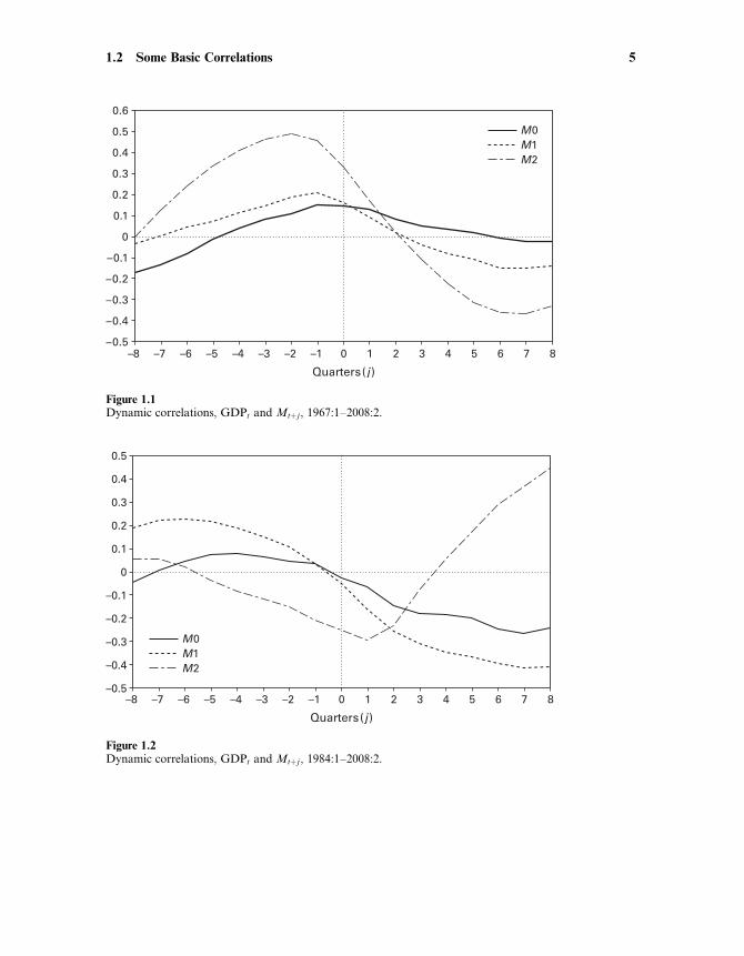
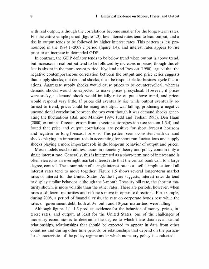
Figure 1.2Dynamic correlations, GDPt and Mtþ j , 1984:1–2008:2.

Figure 1.1Dynamic correlations, GDPt and Mtþ j , 1967:1–2008:2.

1.2 Some Basic Correlations 5

GDP and three di¤erent monetary aggregates, each also in detrended log form.7

Data are quarterly from 1967:1 to 2008:2, and the figures plot, for the entire sample

and for the subperiod 1984:1–2008:2, the correlation between real GDPt and Mtþj

against j, where M represents a monetary aggregate. The three aggregates are the

monetary base (sometimes denoted M0), M1, and M2. M0 is a narrow definition of

the money supply, consisting of total reserves held by the banking system plus cur-

rency in the hands of the public. M1 consists of currency held by the nonbank public,

travelers checks, demand deposits, and other checkable deposits. M2 consists of M1

plus savings accounts and small-denomination time deposits plus balances in retail

money market mutual funds. The post-1984 period is shown separately because

1984 often is identified as the beginning of a period characterized by greater macro-

economic stability, at least until the onset of the financial crisis in 2007.8

As figure 1.1 shows, the correlations with real output change substantially as one

moves from M0 to M2. The narrow measure M0 is positively correlated with real

GDP at both leads and lags over the entire period, but future M0 is negatively corre-

lated with real GDP in the period since 1984. M1 and M2 are positively correlated

at lags but negatively correlated at leads over the full sample. In other words, high

GDP (relative to trend) tends to be preceded by high values of M1 and M2 but fol-

lowed by low values. The positive correlation between GDPt and Mtþj for j < 0

indicates that movements in money lead movements in output. This timing pattern

played an important role in M. Friedman and Schwartz’s classic and highly influen-

tial A Monetary History of the United States (1963a). The larger correlations between

GDP and M2 arise in part from the endogenous nature of an aggregate such as M2,

depending as it does on banking sector behavior as well as on that of the nonbank

private sector (see King and Plosser 1984; Coleman 1996). However, these patterns

for M2 are reversed in the later period, though M1 still leads GDP. Correlations

among endogenous variables reflect the structure of the economy, the nature of

shocks experienced during each period, and the behavior of monetary policy. One

objective of a structural model of the economy and a theory of monetary policy is

to provide a framework for understanding why these dynamic correlations di¤er

over di¤erent periods.

Figures 1.3 and 1.4 show the cross-correlations between detrended real GDP and

several interest rates and between detrended real GDP and the detrended GDP defla-

tor. The interest rates range from the federal funds rate, an overnight interbank rate

used by the Federal Reserve to implement monetary policy, to the 1-year and 10-year

rates on government bonds. The three interest rate series display similar correlations

7. Trends are estimated using a Hodrick-Prescott filter.

8. Perhaps reflecting the greater volatility during 1967–1983, cross-correlations during this period are sim-ilar to those obtained using the entire 1967–2008 period.

6 1 Empirical Evidence on Money, Prices, and Output

Figure 1.3Dynamic correlations, output, prices, and interest rates, 1967:1–2008:2.

Figure 1.4Dynamic correlations, output, prices, and interest rates, 1984:1–2008:2.

1.2 Some Basic Correlations 7

with real output, although the correlations become smaller for the longer-term rates.

For the entire sample period (figure 1.3), low interest rates tend to lead output, and a

rise in output tends to be followed by higher interest rates. This pattern is less pro-

nounced in the 1984:1–2008:2 period (figure 1.4), and interest rates appear to rise

prior to an increase in detrended GDP.

In contrast, the GDP deflator tends to be below trend when output is above trend,

but increases in real output tend to be followed by increases in prices, though this ef-

fect is absent in the more recent period. Kydland and Prescott (1990) argued that the

negative contemporaneous correlation between the output and price series suggests

that supply shocks, not demand shocks, must be responsible for business cycle fluctu-

ations. Aggregate supply shocks would cause prices to be countercyclical, whereas

demand shocks would be expected to make prices procyclical. However, if prices

were sticky, a demand shock would initially raise output above trend, and prices

would respond very little. If prices did eventually rise while output eventually re-

turned to trend, prices could be rising as output was falling, producing a negative

unconditional correlation between the two even though it was demand shocks gener-

ating the fluctuations (Ball and Mankiw 1994; Judd and Trehan 1995). Den Haan

(2000) examined forecast errors from a vector autoregression (see section 1.3.4) and

found that price and output correlations are positive for short forecast horizons

and negative for long forecast horizons. This pattern seems consistent with demand

shocks playing an important role in accounting for short-run fluctuations and supply

shocks playing a more important role in the long-run behavior of output and prices.

Most models used to address issues in monetary theory and policy contain only a

single interest rate. Generally, this is interpreted as a short-term rate of interest and is

often viewed as an overnight market interest rate that the central bank can, to a large

degree, control. The assumption of a single interest rate is a useful simplification if all

interest rates tend to move together. Figure 1.5 shows several longer-term market

rates of interest for the United States. As the figure suggests, interest rates do tend

to display similar behavior, although the 3-month Treasury bill rate, the shortest ma-

turity shown, is more volatile than the other rates. There are periods, however, when

rates at di¤erent maturities and riskiness move in opposite directions. For example,

during 2008, a period of financial crisis, the rate on corporate bonds rose while the

rates on government debt, both at 3-month and 10-year maturities, were falling.

Although figures 1.1–1.5 produce evidence for the behavior of money, prices, in-

terest rates, and output, at least for the United States, one of the challenges of

monetary economics is to determine the degree to which these data reveal causal

relationships, relationships that should be expected to appear in data from other

countries and during other time periods, or relationships that depend on the particu-

lar characteristics of the policy regime under which monetary policy is conducted.

8 1 Empirical Evidence on Money, Prices, and Output

1.3 Estimating the E¤ect of Money on Output

Almost all economists accept that the long-run e¤ects of money fall entirely, or al-

most entirely, on prices, with little impact on real variables, but most economists

also believe that monetary disturbances can have important e¤ects on real variables

such as output in the short run.9 As Lucas (1996) put it in his Nobel lecture, ‘‘This

tension between two incompatible ideas—that changes in money are neutral unit

changes and that they induce movements in employment and production in the

same direction—has been at the center of monetary theory at least since Hume

wrote’’ (664).10 The time series correlations presented in the previous section suggest

the short-run relationships between money and income, but the evidence for the

e¤ects of money on real output is based on more than these simple correlations.

The tools that have been employed to estimate the impact of monetary policy have

evolved over time as the result of developments in time series econometrics and

changes in the specific questions posed by theoretical models. This section reviews

some of the empirical evidence on the relationship between monetary policy and

U.S. macroeconomic behavior. One objective of this literature has been to determine

Figure 1.5Interest rates, 1967:01–2008:09.

9. For an exposition of the view that monetary factors have not played an important role in U.S. businesscycles, see Kydland and Prescott (1990).

10. The reference is to David Hume’s 1752 essays Of Money and Of Interest.

1.3 Estimating the E¤ect of Money on Output 9

whether monetary policy disturbances actually have played an important role in U.S.

economic fluctuations. Equally important, the empirical evidence is useful in judging

whether the predictions of di¤erent theories about the e¤ects of monetary policy are

consistent with the evidence. Among the excellent recent discussions of these issues

are Leeper, Sims, and Zha (1996) and Christiano, Eichenbaum, and Evans (1999),

where the focus is on the role of identified VARs in estimating the e¤ects of mone-

tary policy, and R. King and Watson (1996), where the focus is on using empirical

evidence to distinguish among competing business-cycle models.

1.3.1 The Evidence of Friedman and Schwartz

M. Friedman and Schwartz’s (1963a) study of the relationship between money and

business cycles still represents probably the most influential empirical evidence that

money does matter for business cycle fluctuations. Their evidence, based on almost

100 years of data from the United States, relies heavily on patterns of timing; system-

atic evidence that money growth rate changes lead changes in real economic activity

is taken to support a causal interpretation in which money causes output fluctua-

tions. This timing pattern shows up most clearly in figure 1.1 with M2.

Friedman and Schwartz concluded that the data ‘‘decisively support treating the

rate of change series [of the money supply] as conforming to the reference cycle pos-

itively with a long lead’’ (36). That is, faster money growth tends to be followed by

increases in output above trend, and slowdowns in money growth tend to be fol-

lowed by declines in output. The inference Friedman and Schwartz drew was that

variations in money growth rates cause, with a long (and variable) lag, variations in

real economic activity.

The nature of this evidence for the United States is apparent in figure 1.6, which

shows two detrended money supply measures and real GDP. The monetary aggre-

gates in the figure, M1 and M2, are quarterly observations on the deviations of the

actual series from trend. The sample period is 1967:1–2008:2, so that is after the pe-

riod of the Friedman and Schwartz study. The figure reveals slowdowns in money

leading most business cycle downturns through the early 1980s. However, the pattern

is not so apparent after 1982. B. Friedman and Kuttner (1992) documented the seem-

ing breakdown in the relationship between monetary aggregates and real output; this

changing relationship between money and output has a¤ected the manner in which

monetary policy has been conducted, at least in the United States (see chapter 11).

While it is suggestive, evidence based on timing patterns and simple correlations

may not indicate the true causal role of money. Since the Federal Reserve and the

banking sector respond to economic developments, movements in the monetary

aggregates are not exogenous, and the correlation patterns need not reflect any

causal e¤ect of monetary policy on economic activity. If, for example, the central

10 1 Empirical Evidence on Money, Prices, and Output

bank is implementing monetary policy by controlling the value of some short-term

market interest rate, the nominal stock of money will be a¤ected both by policy

actions that change interest rates and by developments in the economy that are not

related to policy actions. An economic expansion may lead banks to expand lending

in ways that produce an increase in the stock of money, even if the central bank has

not changed its policy. If the money stock is used to measure monetary policy, the

relationship observed in the data between money and output may reflect the impact

of output on money, not the impact of money and monetary policy on output.

Tobin (1970) was the first to model formally the idea that the positive correlation

between money and output—the correlation that Friedman and Schwartz interpreted

as providing evidence that money caused output movements—could in fact reflect

just the opposite—output might be causing money. A more modern treatment of

what is known as the reverse causation argument was provided by R. King and

Plosser (1984). They show that inside money, the component of a monetary aggre-

gate such as M1 that represents the liabilities of the banking sector, is more highly

correlated with output movements in the United States than is outside money, the

liabilities of the Federal Reserve. King and Plosser interpreted this finding as evi-

dence that much of the correlation between broad aggregates such as M1 or M2

and output arises from the endogenous response of the banking sector to economic

disturbances that are not the result of monetary policy actions. More recently, Cole-

man (1996), in an estimated equilibrium model with endogenous money, found that

Figure 1.6Detrended money and real GDP, 1967:1–2008:2.

1.3 Estimating the E¤ect of Money on Output 11

the implied behavior of money in the model cannot match the lead-lag relationship

in the data. Specifically, a money supply measure such as M2 leads output, whereas

Coleman found that his model implies that money should be more highly correlated

with lagged output than with future output.11

The endogeneity problem is likely to be particularly severe if the monetary author-

ity has employed a short-term interest rate as its main policy instrument, and this has

generally been the case in the United States. Changes in the money stock will then be

endogenous and cannot be interpreted as representing policy actions. Figure 1.7

shows the behavior of two short-term nominal interest rates, the 3-month Treasury

bill rate (3MTB) and the federal funds rate, together with detrended real GDP. Like

figure 1.6, figure 1.7 provides some support for the notion that monetary policy

actions have contributed to U.S. business cycles. Interest rates have typically

increased prior to economic downturns. But whether this is evidence that monetary

policy has caused or contributed to cyclical fluctuations cannot be inferred from the

figure; the movements in interest rates may simply reflect the Fed’s response to the

state of the economy.

Simple plots and correlations are suggestive, but they cannot be decisive. Other

factors may be the cause of the joint movements of output, monetary aggregates,

Figure 1.7Interest rates and detrended real GDP, 1967:1–2008:2.

11. Lacker (1988) showed how the correlations between inside money and future output could also arise ifmovements in inside money reflect new information about future monetary policy.

12 1 Empirical Evidence on Money, Prices, and Output

and interest rates. The comparison with business cycle reference points also ignores

much of the information about the time series behavior of money, output, and inter-

est rates that could be used to determine what impact, if any, monetary policy has on

output. And the appropriate variable to use as a measure of monetary policy will de-

pend on how policy has been implemented.

One of the earliest time series econometric attempts to estimate the impact of

money was due to M. Friedman and Meiselman (1963). Their objective was to test

whether monetary or fiscal policy was more important for the determination of nom-

inal income. To address this issue, they estimated the following equation:12

ynt 1 yt þ pt ¼ yn

0 þXi¼0

aiAt�i þXi¼0

bimt�i þXi¼0

hizt�i þ ut; ð1:1Þ

where yn denotes the log of nominal income, equal to the sum of the logs of output

and the price level, A is a measure of autonomous expenditures, and m is a monetary

aggregate; z can be thought of as a vector of other variables relevant for explaining

nominal income fluctuations. Friedman and Meiselman reported finding a much

more stable and statistically significant relationship between output and money than

between output and their measure of autonomous expenditures. In general, they

could not reject the hypothesis that the ai coe‰cients were zero, while the bi coe‰-

cients were always statistically significant.

The use of equations such as (1.1) for policy analysis was promoted by a number

of economists at the Federal Reserve Bank of St. Louis, so regressions of nominal

income on money are often called St. Louis equations (see L. Andersen and Jordon

1968; B. Friedman 1977a; Carlson 1978). Because the dependent variable is nominal

income, the St. Louis approach does not address directly the question of how a

money-induced change in nominal spending is split between a change in real output

and a change in the price level. The impact of money on nominal income was esti-

mated to be quite strong, and Andersen and Jordon (1968, 22) concluded, ‘‘Finding

of a strong empirical relationship between economic activity and . . . monetary actions

points to the conclusion that monetary actions can and should play a more promi-

nent role in economic stabilization than they have up to now.’’13

12. This is not exactly correct; because Friedman and Meiselman included ‘‘autonomous’’ expenditures asan explanatory variable, they also used consumption as the dependent variable (basically, output minusautonomous expenditures). They also reported results for real variables as well as nominal ones. Followingmodern practice, (1.1) is expressed in terms of logs; Friedman and Meiselman estimated their equation inlevels.

13. B. Friedman (1977a) argued that updated estimates of the St. Louis equation did yield a role for fiscalpolicy, although the statistical reliability of this finding was questioned by Carlson (1978). Carlson alsoprovided a bibliography listing many of the papers on the St. Louis equation (see his footnote 2, p. 13).

1.3 Estimating the E¤ect of Money on Output 13

The original Friedman-Meiselman result generated responses by Modigliani and

Ando (1976) and De Prano and Mayer (1965), among others. This debate empha-

sized that an equation such as (1.1) is misspecified if m is endogenous. To illustrate

the point with an extreme example, suppose that the central bank is able to manipu-

late the money supply to o¤set almost perfectly shocks that would otherwise generate

fluctuations in nominal income. In this case, yn would simply reflect the random

control errors the central bank had failed to o¤set. As a result, m and yn might be

completely uncorrelated, and a regression of yn on m would not reveal that money

actually played an important role in a¤ecting nominal income. If policy is able to re-

spond to the factors generating the error term ut, then mt and ut will be correlated,

ordinary least-squares estimates of (1.1) will be inconsistent, and the resulting esti-

mates will depend on the manner in which policy has induced a correlation between

u and m. Changes in policy that altered this correlation would also alter the least-

squares regression estimates one would obtain in estimating (1.1).

1.3.2 Granger Causality

The St. Louis equation related nominal output to the past behavior of money. Simi-

lar regressions employing real output have also been used to investigate the connec-

tion between real economic activity and money. In an important contribution, Sims

(1972) introduced the notion of Granger causality into the debate over the real e¤ects

of money. A variable X is said to Granger-cause Y if and only if lagged values of X

have marginal predictive content in a forecasting equation for Y . In practice, testing

whether money Granger-causes output involves testing whether the ai coe‰cients

equal zero in a regression of the form

yt ¼ y0 þXi¼1

aimt�i þXi¼1

biyt�i þXi¼1

cizt�i þ et; ð1:2Þ

where key issues involve the treatment of trends in output and money, the choice of

lag lengths, and the set of other variables (represented by z) that are included in the

equation.

Sims’s original work used log levels of U.S. nominal GNP and money (both M1

and the monetary base). He found evidence that money Granger-caused GNP. That

is, the past behavior of money helped to predict future GNP. However, using the in-

dex of industrial production to measure real output, Sims (1980) found that the frac-

tion of output variation explained by money was greatly reduced when a nominal

interest rate was added to the equation (so that z consists of the log price level and

an interest rate). Thus, the conclusion seemed sensitive to the specification of z.

Eichenbaum and Singleton (1987) found that money appeared to be less important

if the regressions were specified in log first di¤erence form rather than in log levels

14 1 Empirical Evidence on Money, Prices, and Output

with a time trend. Stock and Watson (1989) provided a systematic treatment of the

trend specification in testing whether money Granger-causes real output. They con-

cluded that money does help to predict future output (they actually used industrial

production) even when prices and an interest rate are included.

A large literature has examined the value of monetary indicators in forecasting

output. One interpretation of Sims’s finding was that including an interest rate

reduces the apparent role of money because, at least in the United States, a short-

term interest rate rather than the money supply provides a better measure of mone-

tary policy actions (see chapter 11). B. Friedman and Kuttner (1992) and Bernanke

and Blinder (1992), among others, looked at the role of alternative interest rate mea-

sures in forecasting real output. Friedman and Kuttner examined the e¤ects of alter-

native definitions of money and di¤erent sample periods and concluded that the

relationship in the United States is unstable and deteriorated in the 1990s. Bernanke

and Blinder found that the federal funds rate ‘‘dominates both money and the bill

and bond rates in forecasting real variables.’’

Regressions of real output on money were also popularized by Barro (1977; 1978;

1979b) as a way of testing whether only unanticipated money matters for real out-

put. By dividing money into anticipated and unanticipated components, Barro ob-

tained results suggesting that only the unanticipated part a¤ects real variables (see

also Barro and Rush 1980 and the critical comment by Small 1979). Subsequent

work by Mishkin (1982) found a role for anticipated money as well. Cover (1992)

employed a similar approach and found di¤erences in the impacts of positive and

negative monetary shocks. Negative shocks were estimated to have significant e¤ects

on output, whereas the e¤ect of positive shocks was usually small and statistically

insignificant.

1.3.3 Policy Uses

Before reviewing other evidence on the e¤ects of money on output, it is useful to ask

whether equations such as (1.2) can be used for policy purposes. That is, can a re-

gression of this form be used to design a policy rule for setting the central bank’s pol-

icy instrument? If it can, then the discussions of theoretical models that form the bulk

of this book would be unnecessary, at least from the perspective of conducting mon-

etary policy.

Suppose that the estimated relationship between output and money takes the form

yt ¼ y0 þ a0mt þ a1mt�1 þ c1zt þ c2zt�1 þ ut: ð1:3Þ

According to (1.3), systematic variations in the money supply a¤ect output. Consider

the problem of adjusting the money supply to reduce fluctuations in real output. If

this objective is interpreted to mean that the money supply should be manipulated

to minimize the variance of yt around y0, then mt should be set equal to

1.3 Estimating the E¤ect of Money on Output 15

mt ¼ � a1

a0mt�1 �

c2

a0zt�1 þ vt

¼ p1mt�1 þ p2zt�1 þ vt; ð1:4Þ

where for simplicity it is assumed that the monetary authority’s forecast of zt is equal

to zero. The term vt represents the control error experienced by the monetary author-

ity in setting the money supply. Equation (1.4) represents a feedback rule for the

money supply whose parameters are themselves determined by the estimated coe‰-

cients in the equation for y. A key assumption is that the coe‰cients in (1.3) are in-

dependent of the choice of the policy rule for m. Substituting (1.4) into (1.3), output

under the policy rule given in (1.4) would be equal to yt ¼ y0 þ c1zt þ ut þ a0vt.

Notice that a policy rule has been derived using only knowledge of the policy ob-

jective (minimizing the expected variance of output) and knowledge of the estimated

coe‰cients in (1.3). No theory of how monetary policy actually a¤ects the economy

was required. Sargent (1976) showed, however, that the use of (1.3) to derive a policy

feedback rule may be inappropriate. To see why, suppose that real output actually

depends only on unpredicted movements in the money supply; only surprises matter,

with predicted changes in money simply being reflected in price level movements with

no impact on output.14 From (1.4), the unpredicted movement in mt is just vt, so let

the true model for output be

yt ¼ y0 þ d0vt þ d1zt þ d2zt�1 þ ut: ð1:5Þ

Now from (1.4), vt ¼ mt � ðp1mt�1 þ p2zt�1Þ, so output can be expressed equiva-

lently as

yt ¼ y0 þ d0½mt � ðp1mt�1 þ p2zt�1Þ� þ d1zt þ d2zt�1 þ ut

¼ y0 þ d0mt � d0p1mt�1 þ d1zt þ ðd2 � d0p2Þzt�1 þ ut; ð1:6Þ

which has exactly the same form as (1.3). Equation (1.3), which was initially inter-

preted as consistent with a situation in which systematic feedback rules for monetary

policy could a¤ect output, is observationally equivalent to (1.6), which was derived

under the assumption that systematic policy had no e¤ect and only money surprises

mattered. The two are observationally equivalent because the error term in both (1.3)

and (1.6) is just ut; both equations fit the data equally well.

A comparison of (1.3) and (1.6) reveals another important conclusion. The coe‰-

cients of (1.6) are functions of the parameters in the policy rule (1.4). Thus, changes

in the conduct of policy, interpreted to mean changes in the feedback rule parame-

14. The influential model of Lucas (1972) has this implication. See chapter 5.

16 1 Empirical Evidence on Money, Prices, and Output

ters, will change the parameters estimated in an equation such as (1.6) (or in a St.

Louis–type regression). This is an example of the Lucas (1976) critique: empirical

relationships are unlikely to be invariant to changes in policy regimes.

Of course, as Sargent stressed, it may be that (1.3) is the true structure that re-

mains invariant as policy changes. In this case, (1.5) will not be invariant to changes

in policy. To demonstrate this point, note that (1.4) implies

mt ¼ ð1� p1LÞ�1ðp2zt�1 þ vtÞ;

where L is the lag operator.15 Hence, we can write (1.3) as

yt ¼ y0 þ a0mt þ a1mt�1 þ c1zt þ c2zt�1 þ ut

¼ y0 þ a0ð1� p1LÞ�1ðp2zt�1 þ vtÞ

þ a1ð1� p1LÞ�1ðp2zt�2 þ vt�1Þ þ c1zt þ c2zt�1 þ ut

¼ ð1� p1Þy0 þ p1yt�1 þ a0vt þ a1vt�1 þ c1zt

þ ðc2 þ a0p2 � c1p1Þzt�1 þ ða1p2 � c2p1Þzt�2 þ ut � p1ut�1; ð1:7Þ

where output is now expressed as a function of lagged output, the z variable, and

money surprises (the v realizations). If this were interpreted as a policy-invariant ex-

pression, one would conclude that output is independent of any predictable or sys-

tematic feedback rule for monetary policy; only unpredicted money appears to

matter. Yet, under the hypothesis that (1.3) is the true invariant structure, changes

in the policy rule (the p1 coe‰cients) will cause the coe‰cients in (1.7) to change.

Note that starting with (1.5) and (1.4), one derives an expression for output that is

observationally equivalent to (1.3). But starting with (1.3) and (1.4), one ends up with

an expression for output that is not equivalent to (1.5); (1.7) contains lagged values

of output, v, and u, and two lags of z, whereas (1.5) contains only the contemporane-

ous values of v and u and one lag of z. These di¤erences would allow one to dis-

tinguish between the two, but they arise only because this example placed a priori

restrictions on the lag lengths in (1.3) and (1.5). In general, one would not have the

type of a priori information that would allow this.

The lesson from this simple example is that policy cannot be designed without a

theory of how money a¤ects the economy. A theory should identify whether the coef-

ficients in a specification of the form (1.3) or in a specification such as (1.5) will re-

main invariant as policy changes. While output equations estimated over a single

15. That is, L ixt ¼ xt�i.

1.3 Estimating the E¤ect of Money on Output 17

policy regime may not allow the true structure to be identified, information from sev-

eral policy regimes might succeed in doing so. If a policy regime change means that

the coe‰cients in the policy rule (1.4) have changed, this would serve to identify

whether an expression of the form (1.3) or one of the form (1.5) was policy-invariant.

1.3.4 The VAR Approach

Much of the understanding of the empirical e¤ects of monetary policy on real eco-

nomic activity has come from the use of vector autoregression (VAR) frameworks.

The use of VARs to estimate the impact of money on the economy was pioneered

by Sims (1972; 1980). The development of the approach as it moved from bivariate

(Sims 1972) to trivariate (Sims 1980) to larger and larger systems as well as the em-

pirical findings the literature has produced were summarized by Leeper, Sims, and

Zha (1996). Christiano, Eichenbaum, and Evans (1999) provided a thorough discus-

sion of the use of VARs to estimate the impact of money, and they provided an ex-

tensive list of references to work in this area.16

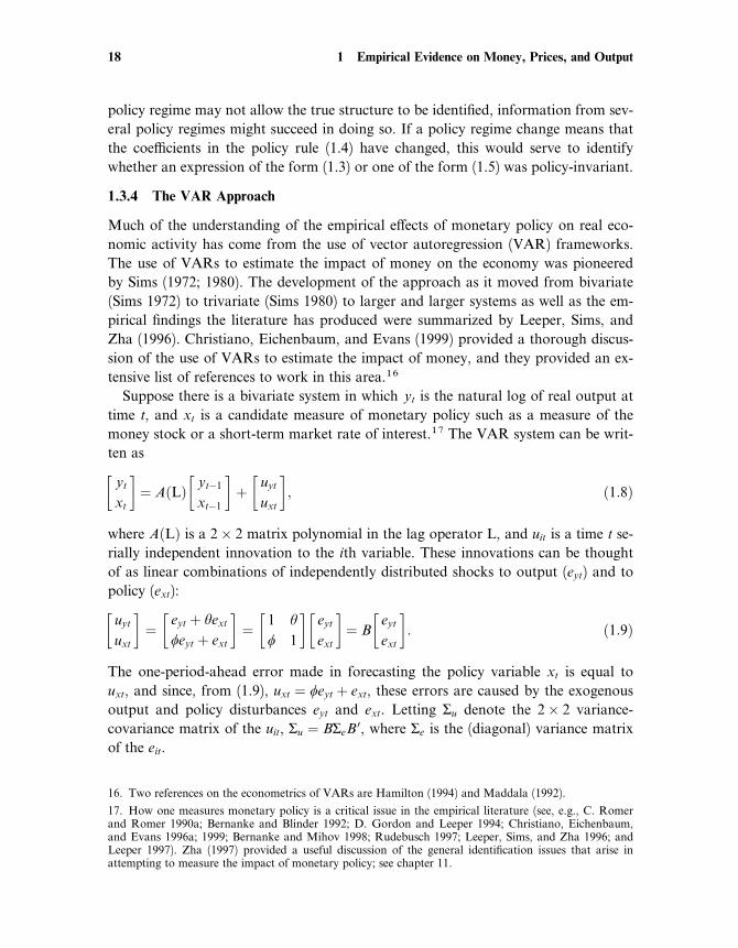
Suppose there is a bivariate system in which yt is the natural log of real output at

time t, and xt is a candidate measure of monetary policy such as a measure of the

money stock or a short-term market rate of interest.17 The VAR system can be writ-

ten as

yt

xt

� �¼ AðLÞ yt�1

xt�1

� �þ uyt

uxt

� �; ð1:8Þ

where AðLÞ is a 2� 2 matrix polynomial in the lag operator L, and uit is a time t se-

rially independent innovation to the ith variable. These innovations can be thought

of as linear combinations of independently distributed shocks to output (eyt) and to

policy (ext):

uyt

uxt

� �¼

eyt þ yext

feyt þ ext

� �¼ 1 y

f 1

� �eyt

ext

� �¼ B

eyt

ext

� �: ð1:9Þ

The one-period-ahead error made in forecasting the policy variable xt is equal to

uxt, and since, from (1.9), uxt ¼ feyt þ ext, these errors are caused by the exogenous

output and policy disturbances eyt and ext. Letting Su denote the 2� 2 variance-

covariance matrix of the uit, Su ¼ BSeB0, where Se is the (diagonal) variance matrix

of the eit.

16. Two references on the econometrics of VARs are Hamilton (1994) and Maddala (1992).

17. How one measures monetary policy is a critical issue in the empirical literature (see, e.g., C. Romerand Romer 1990a; Bernanke and Blinder 1992; D. Gordon and Leeper 1994; Christiano, Eichenbaum,and Evans 1996a; 1999; Bernanke and Mihov 1998; Rudebusch 1997; Leeper, Sims, and Zha 1996; andLeeper 1997). Zha (1997) provided a useful discussion of the general identification issues that arise inattempting to measure the impact of monetary policy; see chapter 11.

18 1 Empirical Evidence on Money, Prices, and Output

The random variable ext represents the exogenous shock to policy. To determine

the role of policy in causing movements in output or other macroeconomic variables,

one needs to estimate the e¤ect of ex on these variables. As long as f0 0, the inno-

vation to the observed policy variable xt will depend both on the shock to policy extand on the nonpolicy shock eyt; obtaining an estimate of uxt does not provide a mea-

sure of the policy shock unless f ¼ 0.

To make the example even more explicit, suppose the VAR system is

yt

xt

� �¼ a1 a2

0 0

� �yt�1

xt�1

� �þ uyt

uxt

� �; ð1:10Þ

with 0 < a1 < 1. Then xt ¼ uxt, and yt ¼ a1yt�1 þ uyt þ a2uxt�1, and one can write ytin moving average form as

yt ¼Xyi¼0

ai1uyt�i þ

Xyi¼0

ai1a2uxt�i�1:

Estimating (1.10) yields estimates of AðLÞ and Su, and from these the e¤ects of uxt on

fyt; ytþ1; . . .g can be calculated. If one interpreted ux as an exogenous policy distur-

bance, then the implied response of yt; ytþ1; . . . to a policy shock would be18

0; a2; a1a2; a21a2; . . . :

To estimate the impact of a policy shock on output, however, one needs to calcu-

late the e¤ect on fyt; ytþ1; . . .g of a realization of the policy shock ext. In terms of the

true underlying structural disturbances ey and ex, (1.9) implies

yt ¼Xyi¼0

ai1ðeyt�i þ yext�iÞ þ

Xyi¼0

ai1a2ðext�i�1 þ feyt�i�1Þ

¼ eyt þXyi¼0

ai1ða1 þ a2fÞeyt�i�1 þ yext þ

Xyi¼0

ai1ða1yþ a2Þext�i�1; ð1:11Þ

so the impulse response function giving the true response of y to the exogenous pol-

icy shock ex is

y; a1yþ a2; a1ða1yþ a2Þ; a21ða1yþ a2Þ; . . . :

18. This represents the response to an nonorthogonalized innovation. The basic point, however, is that if yand f are nonzero, the underlying shocks are not identified, so the estimated response to ux or to the com-ponent of ux that is orthogonal to uy will not identify the response to the policy shock ex.

1.3 Estimating the E¤ect of Money on Output 19

This response involves the elements of AðLÞ and the elements of B. And while AðLÞcan be estimated from (1.8), B and Se are not identified without further restrictions.19

Two basic approaches to solving this identification problem have been followed.

The first imposes additional restrictions on the matrix B that links the observable

VAR residuals to the underlying structural disturbances (see (1.9)). This approach

was used by Sims (1972; 1988); Bernanke (1986); Walsh (1987); Bernanke and

Blinder (1992); D. Gordon and Leeper (1994); and Bernanke and Mihov (1998),

among others. If policy shocks a¤ect output with a lag, for example, the restriction

that y ¼ 0 would allow the other parameters of the model to be identified. The sec-

ond approach achieves identification by imposing restrictions on the long-run e¤ects

of the disturbances on observed variables. For example, the assumption of long-run

neutrality of money would imply that a monetary policy shock (ex) has no long-

run permanent e¤ect on output. In terms of the example that led to (1.11), long-run

neutrality of the policy shock would imply that yþ ða1yþ a2ÞP

ai1 ¼ 0 or y ¼ �a2.

Examples of this approach include Blanchard and Watson (1986); Blanchard (1989);

Blanchard and Quah (1989); Judd and Trehan (1989); Hutchison and Walsh (1992);

and Galı́ (1992). The use of long-run restrictions is criticized by Faust and Leeper

(1997).

In Sims (1972), the nominal money supply (M1) was treated as the measure of

monetary policy (the x variable), and policy shocks were identified by assuming that

f ¼ 0. This approach corresponds to the assumption that the money supply is prede-

termined and that policy innovations are exogenous with respect to the nonpolicy

innovations (see (1.9)). In this case, uxt ¼ ext, so from the fact that uyt ¼ yext þ eyt ¼yuxt þ eyt, y can be estimated from the regression of the VAR residuals uyt on the

VAR residuals uxt.20 This corresponds to a situation in which the policy variable x

does not respond contemporaneously to output shocks, perhaps because of informa-

tion lags in formulating policy. However, if x depends contemporaneously on non-

policy disturbances as well as policy shocks (f0 0), using uxt as an estimate of extwill compound the e¤ects of eyt on uxt with the e¤ects of policy actions.

An alternative approach seeks a policy measure for which y ¼ 0 is a plausible as-

sumption; this corresponds to the assumption that policy shocks have no contempo-

raneous impact on output.21 This type of restriction was imposed by Bernanke and

Blinder (1992) and Bernanke and Mihov (1998). How reasonable such an assump-

tion might be clearly depends on the unit of observation. In annual data, the assump-

19. In this example, the three elements of Su, the two variances and the covariance term, are functions ofthe four unknown parameters, f, y, and the variances of ey and ex.

20. This represents a Choleski decomposition of the VAR residuals with the policy variable ordered first.

21. This represents a Choleski decomposition with output ordered before the policy variable.

20 1 Empirical Evidence on Money, Prices, and Output

tion of no contemporaneous e¤ect would be implausible; with monthly data, it might

be much more plausible.

This discussion has, for simplicity, treated both y and x as scalars. In fact, neither

assumption is appropriate. One is usually interested in the e¤ects of policy on several

dimensions of an economy’s macroeconomic performance, and policy is likely to re-

spond to unemployment and inflation as well as to other variables, so y would nor-

mally be a vector of nonpolicy variables. Then the restrictions that correspond to

either f ¼ 0 or y ¼ 0 may be less easily justified. While one might argue that policy

does not respond contemporaneously to unemployment when the analysis involves

monthly data, this is not likely to be the case with respect to market interest rates.

And, using the same example, one might be comfortable assuming that the current

month’s unemployment rate is una¤ected by current policy actions, but this would

not be true of interest rates, since financial markets will respond immediately to pol-

icy actions.

In addition, there generally is no clear scalar choice for the policy variable x. If

policy were framed in terms of strict targets for the money supply, for a specific mea-

sure of banking sector reserves, or for a particular short-term interest rate, then the

definition of x might be straightforward. In general, however, several candidate mea-

sures of monetary policy will be available, all depending in various degrees on both

policy actions and nonpolicy disturbances. What constitutes an appropriate candi-

date for x, and how x depends on nonpolicy disturbances, will depend on the operat-

ing procedures the monetary authority is following as it implements policy.

Money and Output

Sims (1992) provided a useful summary of the VAR evidence on money and output

from France, Germany, Japan, the United Kingdom, and the United States. He esti-

mated separate VARs for each country, using a common specification that includes

industrial production, consumer prices, a short-term interest rate as the measure of

monetary policy, a measure of the money supply, an exchange rate index, and an

index of commodity prices. Sims ordered the interest rate variable first. This cor-

responds to the assumption that f ¼ 0; innovations to the interest rate variable po-

tentially a¤ect the other variables contemporaneously (Sims used monthly data),

whereas the interest rate is not a¤ected contemporaneously by innovations in any of

the other variables.22

The response of real output to an interest rate innovation was similar for all five of

the countries Sims examined. In all cases, monetary shocks led to an output response

that is usually described as following a hump-shaped pattern. The negative output

22. Sims noted that the correlations among the VAR residuals, the u 0it, are small so that the ordering has

little impact on his results (i.e., sample estimates of f and y are small).

1.3 Estimating the E¤ect of Money on Output 21

e¤ects of a contractionary shock, for example, build to a peak after several months

and then gradually die out.

Eichenbaum (1992) compared the estimated e¤ects of monetary policy in the

United States using alternative measures of policy shocks and discussed how di¤erent

choices can produce puzzling results, at least puzzling relative to certain theoretical

expectations. He based his discussion on the results obtained from a VAR containing

four variables: the price level and output (these correspond to the elements of y in

(1.8)), M1 as a measure of the money supply, and the federal funds rate as a measure

of short-term interest rates (these correspond to the elements of x). He considered

interpreting shocks to M1 as policy shocks versus the alternative of interpreting

funds rate shocks as policy shocks. He found that a positive innovation to M1 is fol-

lowed by an increase in the federal funds rate and a decline in output. This result is

puzzling if M1 shocks are interpreted as measuring the impact of monetary policy.

An expansionary monetary policy shock would be expected to lead to increases in

both M1 and output. The interest rate was also found to rise after a positive M1

shock, also a potentially puzzling result; a standard model in which money demand

varies inversely with the nominal interest rate would suggest that an increase in the

money supply would require a decline in the nominal rate to restore money market

equilibrium. D. Gordon and Leeper (1994) showed that a similar puzzle emerges

when total reserves are used to measure monetary policy shocks. Positive reserve

innovations are found to be associated with increases in short-term interest rates

and unemployment increases. The suggestion that a rise in reserves or the money

supply might raise, not lower, market interest rates generated a large literature

that attempted to search for a liquidity e¤ect of changes in the money supply (e.g.,

Reichenstein 1987; Christiano and Eichenbaum 1992a; Leeper and Gordon 1992;

Strongin 1995; Hamilton 1996).

When Eichenbaum used innovations in the short-term interest rate as a measure of

monetary policy actions, a positive shock to the funds rate represented a contrac-

tionary policy shock. No output puzzle was found in this case; a positive interest

rate shock was followed by a decline in the output measure. Instead, what has been

called the price puzzle emerges: a contractionary policy shock is followed by a rise in

the price level. The e¤ect is small and temporary (and barely statistically significant)

but still puzzling. The most commonly accepted explanation for the price puzzle is

that it reflects the fact that the variables included in the VAR do not span the full

information set available to the Fed. Suppose the Fed tends to raise the funds rate

whenever it forecasts that inflation might rise in the future. To the extent that the

Fed is unable to o¤set the factors that led it to forecast higher inflation, or to the ex-

tent that the Fed acts too late to prevent inflation from rising, the increase in the

funds rate will be followed by a rise in prices. This interpretation would be consistent

22 1 Empirical Evidence on Money, Prices, and Output

with the price puzzle. One solution is to include commodity prices or other asset pri-

ces in the VAR. Since these prices tend to be sensitive to changing forecasts of future

inflation, they serve as a proxy for some of the Fed’s additional information (Sims

1992; Chari, Christiano, and Eichenbaum 1995; Bernanke and Mihov 1998). Sims

(1992) showed that the price puzzle is not confined to U.S. studies. He reported

VAR estimates of monetary policy e¤ects for France, Germany, Japan, and the

United Kingdom as well as for the United States, and in all cases a positive shock

to the interest rate led to a positive price response. These price responses tended to

become smaller, but did not in all cases disappear, when a commodity price index

and a nominal exchange rate were included in the VAR.

An alternative interpretation of the price puzzle is provided by Barth and Ramey

(2002). They argued that contractionary monetary policy operates on aggregate sup-

ply as well as aggregate demand. For example, an increase in interest rates raises the

cost of holding inventories and thus acts as a positive cost shock. This negative sup-

ply e¤ect raises prices and lowers output. Such an e¤ect is called the cost channel

of monetary policy. In this interpretation, the price puzzle is simply evidence of the

cost channel rather than evidence that the VAR is misspecified. Barth and Ramey

combined industry-level data with aggregate data in a VAR and reported evidence

supporting the cost channel interpretation of the price puzzle (see also Ravenna and

Walsh 2006).

One di‰culty in measuring the impact of monetary policy shocks arises when

operating procedures change over time. The best measure of policy during one period

may no longer accurately reflect policy in another period if the implementation of

policy has changed. Many authors have argued that over most of the past 35 years,

the federal funds rate has been the key policy instrument in the United States, sug-

gesting that unforecasted changes in this interest rate may provide good estimates of

policy shocks. This view has been argued, for example, by Bernanke and Blinder

(1992) and Bernanke and Mihov (1998). While the Fed’s operating procedures have

varied over time, the funds rate is likely to be the best indicator of policy in the

United States during the pre-1979 and post-1982 periods.23 Policy during the period

1979–1982 is less adequately characterized by the funds rate.24

While researchers have disagreed on the best means of identifying policy shocks,

there has been a surprising consensus on the general nature of the economic re-

sponses to monetary policy shocks. A variety of VARs estimated for a number of

23. Chapter 11 provides a brief history of Fed operating procedures.

24. During this period, nonborrowed reserves were set to achieve a level of interest rates consistent withthe desired monetary growth targets. In this case, the funds rate may still provide a satisfactory policy in-dicator. Cook (1989) found that most changes in the funds rate during the 1979–1982 period reflected pol-icy actions. See chapter 11 for a discussion of operating procedures and the reserve market.

1.3 Estimating the E¤ect of Money on Output 23

countries all indicate that in response to a policy shock, output follows a hump-

shaped pattern in which the peak impact occurs several quarters after the initial

shock. Monetary policy actions appear to be taken in anticipation of inflation, so

that a price puzzle emerges if forward-looking variables such as commodity prices

are not included in the VAR.

If monetary policy shocks cause output movements, how important have these

shocks been in accounting for actual business cycle fluctuations? Leeper, Sims, and

Zha (1996) concluded that monetary policy shocks have been relatively unimportant.

However, their assessment is based on monthly data for the period from the begin-

ning of 1960 until early 1996. This sample contains several distinct periods character-

ized by di¤erences in the procedures used by the Fed to implement monetary policy,

and the contribution of monetary shocks may have di¤ered over various subperiods.

Christiano, Eichenbaum, and Evans (1999) concluded that estimates of the impor-

tance of monetary policy shocks for output fluctuations are sensitive to the way mon-

etary policy is measured. When they used a funds-rate measure of monetary policy,

policy shocks accounted for 21 percent of the four-quarter-ahead forecast error vari-

ance for quarterly real GDP. This figure rose to 38 percent of the 12-quarter-ahead

forecast error variance. Smaller e¤ects were found using policy measures based on

monetary aggregates. Christiano, Eichenbaum, and Evans found that very little of

the forecast error variance for the price level could be attributed to monetary policy

shocks.

Criticisms of the VAR Approach

Measures of monetary policy based on the estimation of VARs have been criticized

on several grounds.25 First, some of the impulse responses do not accord with most

economists’ priors. In particular, the price puzzle—the finding that a contractionary

policy shock, as measured by a funds rate shock, tends to be followed by a rise in

the price level—is troublesome. As noted earlier, the price puzzle can be solved by

including oil prices or commodity prices in the VAR system, and the generally

accepted interpretation is that lacking these inflation-sensitive prices, a standard

VAR misses important information that is available to policymakers. A related but

more general point is that many of the VAR models used to assess monetary policy

fail to incorporate forward-looking variables. Central banks look at a lot of informa-

tion in setting policy. Because policy is likely to respond to forecasts of future eco-

nomic conditions, VARs may attribute the subsequent movements in output and

inflation to the policy action. However, the argument that puzzling results indicate

a misspecification implicitly imposes a prior belief about what the correct e¤ects of

25. These criticisms are detailed in Rudebusch (1998).

24 1 Empirical Evidence on Money, Prices, and Output

monetary shocks should look like. Eichenbaum (1992), in fact, argued that short-

term interest rate innovations have been used to represent policy shocks in VARs

because they produce the types of impulse response functions for output that econo-

mists expect.

In addition, the residuals from the VAR regressions that are used to represent ex-

ogenous policy shocks often bear little resemblance to standard interpretations of the

historical record of past policy actions and periods of contractionary and expansion-

ary policy (She¤rin 1995; Rudebusch 1998). They also di¤er considerably depending

on the particular specification of the VAR. Rudebusch (1998) reported low correla-

tions between the residual policy shocks he obtained based on funds rate futures and

those obtained from a VAR by Bernanke and Mihov. How important this finding is

depends on the question of interest. If the objective is to determine whether a partic-

ular recession was caused by a policy shock, then it is important to know if and when

the policy shock occurred. If alternative specifications provide di¤ering and possibly

inconsistent estimates of when policy shocks occurred, then their usefulness as a tool

of economic history would be limited. If, however, the question of interest is how

the economy responds when a policy shock occurs, then the discrepancies among

the VAR residual estimates may be of less importance. Sims (1998a) argued that in

a simple supply-demand model di¤erent authors using di¤erent supply curve shifters

may obtain quite similar estimates of the demand curve slope (since they all obtain

consistent estimators of the true slope). At the same time, they may obtain quite dif-

ferent residuals for the estimated supply curve. If the true interest is in the parameters

of the demand curve, the variations in the estimates of the supply shocks may not be

of importance. Thus, the type of historical analysis based on a VAR, as in Walsh

(1993), is likely to be more problematic than the use of a VAR to determine the

way the economy responds to exogenous policy shocks.

While VARs focus on residuals that are interpreted as policy shocks, the system-

atic part of the estimated VAR equation for a variable such as the funds rate can be

interpreted as a policy reaction function; it provides a description of how the policy

instrument has been adjusted in response to lagged values of the other variables

included in the VAR system. Rudebusch (1998) argued that the implied policy reac-

tion functions look quite di¤erent than results obtained from more direct attempts to

estimate reaction functions or to model actual policy behavior.26 A related point is

that VARs are typically estimated using final, revised data and will therefore not cap-

ture accurately the historical behavior of the monetary policymaker who is reacting

26. For example, Taylor (1993a) employed a simple interest rate rule that closely matches the actual be-havior of the federal funds rate in recent years. As Khoury (1990) noted in a survey of many earlier studiesof the Fed’s reaction function, few systematic conclusions have emerged from this empirical literature.

1.3 Estimating the E¤ect of Money on Output 25

to preliminary and incomplete data. Woolley (1995) showed how the perception of

the stance of monetary policy in the United States in 1972 and President Richard

Nixon’s attempts to pressure Fed Chairman Arthur F. Burns into adopting a more

expansionary policy were based on initial data on the money supply that were sub-

sequently very significantly revised.

At best the VAR approach identifies only the e¤ects of monetary policy shocks,

shifts in policy unrelated to the endogenous response of policy to developments in

the economy. Yet most, if not all, of what one thinks of in terms of policy and policy

design represents the endogenous response of policy to the economy, and ‘‘most vari-

ation in monetary policy instruments is accounted for by responses of policy to the

state of the economy, not by random disturbances to policy’’ (Sims 1998a, 933). So

it is unfortunate that a primary empirical tool—VAR analysis—used to assess the

impact of monetary policy is uninformative about the role played by policy rules. If

policy is completely characterized as a feedback rule on the economy, so that there

are no exogenous policy shocks, then the VAR methodology would conclude that

monetary policy doesn’t matter. Yet while monetary policy is not causing output

movements in this example, it does not follow that policy is unimportant; the re-

sponse of the economy to nonpolicy shocks may depend importantly on the way

monetary policy endogenously adjusts.

Cochrane (1998) made a similar point related to the issues discussed in section

1.3.3. In that section, it was noted that one must know whether it is anticipated

money that has real e¤ects (as in (1.3)) or unanticipated money that matters (as in

(1.5)). Cochrane argued that while most of the VAR literature has focused on issues

of lag length, detrending, ordering, and variable selection, there is another funda-

mental identification issue that has been largely ignored—is it anticipated or un-

anticipated monetary policy that matters? If only unanticipated policy matters, then

the subsequent systematic behavior of money after a policy shock is irrelevant. This

means that the long hump-shaped response of real variables to a policy shock must

be due to inherent lags of adjustment and the propagation mechanisms that charac-

terize the structure of the economy. If anticipated policy matters, then subsequent

systematic behavior of money after a policy shock is relevant. This means that the

long hump-shaped response of real variables to a policy shock may only be present

because policy shocks are followed by persistent, systematic policy actions. If this is

the case, the direct impact of a policy shock, if it were not followed by persistent pol-

icy moves, would be small.

Attempts have been made to use VAR frameworks to assess the systematic e¤ects

of monetary policy. Sims (1998b), for example, estimated a VAR for the interwar

years and used it to simulate the behavior of the economy if policy had been deter-

mined according to the feedback rule obtained from a VAR estimated using postwar

data.

26 1 Empirical Evidence on Money, Prices, and Output

1.3.5 Structural Econometric Models

The empirical assessment of the e¤ects of alternative feedback rules for monetary

policy has traditionally been carried out using structural macroeconometric models.

During the 1960s and early 1970s, the specification, estimation, use, and evaluation

of large-scale econometric models for forecasting and policy analysis represented

a major research agenda in macroeconomics. Important contributions to the under-

standing of investment, consumption, the term structure, and other aspects of the

macroeconomy grew out of the need to develop structural equations for various sec-

tors of the economy. An equation describing the behavior of a policy instrument

such as the federal funds rate was incorporated into these structural models, allow-

ing model simulations of alternative policy rules to be conducted. These simulations

would provide an estimate of the impact on the economy’s dynamic behavior of

changes in the way policy was conducted. For example, a policy under which the

funds rate was adjusted rapidly in response to unemployment movements could be

contrasted with one in which the response was more muted.

A key maintained hypothesis, one necessary to justify this type of analysis, was

that the estimated parameters of the model would be invariant to the specification

of the policy rule. If this were not the case, then one could no longer treat the model’s

parameters as unchanged when altering the monetary policy rule (as the example in

section 1.3.3 shows). In a devastating critique of this assumption, Lucas (1976)

argued that economic theory predicts that the decision rules for investment, con-

sumption, and expectations formation will not be invariant to shifts in the systematic

behavior of policy. The Lucas critique emphasized the problems inherent in the as-

sumption, common in the structural econometric models of the time, that expecta-

tions adjust adaptively to past outcomes.

While large-scale econometric models of aggregate economies continued to play

an important role in discussions of monetary policy, they fell out of favor among

academic economists during the 1970s, in large part as a result of Lucas’s critique,

the increasing emphasis on the role of expectations in theoretical models, and the

dissatisfaction with the empirical treatment of expectations in existing large-scale

models.27 The academic literature witnessed a continued interest in small-scale

rational-expectations models, both single and multicountry versions (for example,

the work of Taylor 1993b), as well as the development of larger-scale models (Fair

1984), all of which incorporated rational expectations into some or all aspects of the

model’s behavioral relationships. Other examples of small models based on rational

expectations and forward-looking behavior include Fuhrer (1994b; 1997c), and

Fuhrer and Moore (1995a; 1995b).

27. For an example of a small-scale model in which expectations play no explicit role, see Rudebusch andSvensson (1997).

1.3 Estimating the E¤ect of Money on Output 27

More recently, empirical work investigating the impact of monetary policy has

relied on estimated dynamic stochastic general equilibrium (DSGE) models. These

models combine rational expectations with a microeconomic foundation in which

households and firms are assumed to behave optimally, given their objectives (utility

maximization, profit maximization) and the constraints they face. Many central

banks have built and estimated DSGE models to use for policy analysis, and many

more central banks are in the process of doing so. Examples of such models include

Adolfson et al. (2007b) for Sweden and Gouvea et al. (2008) for Brazil. In general,

these models are built on the theoretical foundations of the new Keynesian model.

As discussed in chapter 8, this model is based on the assumption that prices and

wages display rigidities and that this nominal stickiness accounts for the real e¤ects

of monetary policy. Early examples include Yun (1996); Ireland (1997a); and Rotem-

berg and Woodford (1998). Among the recent examples of DSGE models are Chris-

tiano, Eichenbaum, and Evans (2005), who estimated the model by matching VAR

impulse responses, and Smets and Wouter (2003), who estimated their model using

Bayesian techniques. The use of Bayesian estimation is now common; recent exam-

ples include Levin et al. (2006); Smets and Wouter (2003; 2007); and Lubik and

Schorfheide (2007).

1.3.6 Alternative Approaches

Although the VAR approach has been the most commonly used empirical methodol-

ogy, and although the results have provided a fairly consistent view of the impact of

monetary policy shocks, other approaches have also influenced views on the role pol-

icy has played. Two such approaches, one based on deriving policy directly from a

reading of policy statements, the other based on case studies of disinflations, have

influenced academic discussions of monetary policy.

Narrative Measures of Monetary Policy

An alternative to the VAR statistical approach is to develop a measure of the stance

of monetary policy from a direct examination of the policy record. In recent years,

this approach has been taken by C. Romer and Romer (1990a) and Boschen and

Mills (1991), among others.28

Boschen and Mills developed an index of policy stance that takes on integer values

from �2 (strong emphasis on inflation reduction) to þ2 (strong emphasis on ‘‘pro-

moting real growth’’). Their monthly index is based on a reading of the Fed’s Fed-

eral Open Market Committee (FOMC) policy directives and the records of the

FOMC meetings. Boschen and Mills showed that innovations in their index corre-

28. Boschen and Mills (1991) provided a discussion and comparison of some other indices of policy. For acritical view of Romer and Romer’s approach, see Leeper (1993).

28 1 Empirical Evidence on Money, Prices, and Output

sponding to expansionary policy shifts are followed by subsequent increases in mon-

etary aggregates and declines in the federal funds rate. They also concluded that all

the narrative indices they examined yield relatively similar conclusions about the im-

pact of policy on monetary aggregates and the funds rates. And in support of the

approach used in section 1.3.4, Boschen and Mills concluded that the funds rate is a

good indicator of monetary policy. These findings are extended in Boschen and Mills

(1995a), which compared several narrative-based measures of monetary policy, find-

ing them to be associated with permanent changes in the level of M2 and the mone-

tary base and temporary changes in the funds rate.

Romer and Romer (1990a) used the Fed’s ‘‘Record of Policy Actions’’ and, prior

to 1976 when they were discontinued, minutes of FOMC meetings to identify epi-

sodes in which policy shifts occurred that were designed to reduce inflation.29 They

found six di¤erent months during the postwar period that saw such contractionary

shifts in Fed policy: October 1947, September 1955, December 1968, April 1974, Au-

gust 1978, and October 1979. Leeper (1993) argued that the Romer-Romer index is

equivalent to a dummy variable that picks up large interest rate innovations. Hoover

and Perez (1994) provided a critical assessment of the Romers’ narrative approach,

noting that the Romer dates are associated with oil price shocks, and Leeper (1997)

found that the exogenous component of the Romers’ policy variable does not pro-

duce dynamic e¤ects on output and prices that accord with general beliefs about the

e¤ects of monetary policy.

The narrative indices of Boschen and Mills and the dating system employed by

Romer and Romer to isolate episodes of contractionary policy provide a useful and

informative alternative to the VAR approach that associates policy shocks with seri-

ally uncorrelated innovations. The VAR approach attempts to identify exogenous

shifts in policy; the estimated e¤ects of these exogenous shifts are the conceptual par-

allels to the comparative static exercises for which theoretical models make predic-

tions. To determine whether the data are consistent with a model’s predictions about

the e¤ects of an exogenous policy action, one needs to isolate empirically such exog-

enous shifts. Doing so, however, does not yield a measure of whether policy is, on

net, expansionary or contractionary.30 The narrative indices can provide a better

measure of the net stance of policy, but they capture both exogenous shifts in policy

and the endogenous response of monetary policy to economic developments. It is

presumably the latter that accounts for most of the observed changes in policy vari-

ables such as the funds rate as policy responds to current and future expected eco-

nomic conditions. In fact, a major conclusion of Leeper, Sims, and Zha (1996), and

one they viewed as not surprising, was that most movements in monetary policy

29. The FMOC resumed publishing its minutes in 2005.

30. Bernanke and Mihov (1998) used their VAR estimates in an attempt to develop such a measure.

1.3 Estimating the E¤ect of Money on Output 29

instruments represent responses to the state of the economy, not exogenous policy

shifts.

Case Studies of Disinflation

Case studies of specific episodes of disinflation provide, in principle, an alternative

means of assessing the real impact of monetary policy. Romer and Romer’s ap-

proach to dating periods of contractionary monetary policy is one form of case

study. However, the most influential example of this approach is that of Sargent

(1986), who examined the ends of several hyperinflations. As discussed more fully in

chapter 5, the distinction between anticipated and unanticipated changes in monetary

policy has played an important role during the past 30 years in academic discussions

of monetary policy, and a key hypothesis is that anticipated changes should a¤ect

prices and inflation with little or no e¤ect on real economic activity. This implies

that a credible policy to reduce inflation should succeed in actually reducing inflation

without causing a recession. This implication contrasts sharply with the view that

any policy designed to reduce inflation would succeed only by inducing an economic

slowdown and temporarily higher unemployment.

Sargent tested these competing hypotheses by examining the ends of the post–

World War I hyperinflations in Austria, German, Hungary, and Poland. In each

case, Sargent found that the hyperinflations ended abruptly. In Austria, for example,

prices rose by over a factor of 20 from December 1921 to August 1922, an annual

inflation rate of over 8800 percent. Prices then stopped rising in September 1922,

actually declining by more than 10 percent during the remainder of 1922. While un-

employment did rise during the price stabilizations, Sargent concluded that the out-

put cost ‘‘was minor compared with the $220 billion GNP that some current analysts

estimate would be lost in the United States per one percentage point inflation reduc-

tion’’ (Sargent 1986, 55). Sargent’s interpretation of the experiences in Germany, Po-

land, and Hungary is similar. In each case, the hyperinflation was ended by a regime

shift that involved a credible change in monetary and fiscal policy designed to reduce

government reliance on inflationary finance. Because the end of inflation reduced the

opportunity cost of holding money, money demand grew and the actual stock of

money continued to grow rapidly after prices had stabilized.

Sargent’s conclusion that the output costs of these disinflations were small has

been questioned, as have the lessons he drew for the moderate inflations experienced

by the industrialized economies in the 1970s and early 1980s. As Sargent noted, the

ends of the hyperinflations ‘‘were not isolated restrictive actions within a given set of

rules of the game’’ but represented changes in the rules of the game, most impor-

tantly in the ability of the fiscal authority to finance expenditures by creating money.

In contrast, the empirical evidence from VARs of the type discussed earlier in this

chapter reflects the impact of policy changes within a given set of rules.

30 1 Empirical Evidence on Money, Prices, and Output

Schelde-Andersen (1992) and Ball (1993) provided more recent examples of the

case study approach. In both cases, the authors examined disinflationary episodes in

order to estimate the real output costs associated with reducing inflation.31 Their

cases, all involving OECD countries, represent evidence on the costs of ending mod-

erate inflations. Ball calculated the deviation of output from trend during a period of

disinflation and expressed this as a ratio to the change in trend inflation over the

same period. The 65 disinflation periods he identified in annual data yield an aver-

age sacrifice ratio of 0.77 percent; each percentage point reduction in inflation was

associated with a 0.77 percent loss of output relative to trend. The estimate for the

United States was among the largest, averaging 2.3 percent based on annual data.

The sacrifice ratios are negatively related to nominal wage flexibility; countries with

greater wage flexibility tend to have smaller sacrifice ratios. The costs of a disinfla-

tion also appear to be larger when inflation is brought down more gradually over a

longer period of time.32

The case study approach can provide interesting evidence on the real e¤ects of

monetary policy. Unfortunately, as with the VAR and other approaches, the issue

of identification needs to be addressed. To what extent have disinflations been exog-

enous, so that any resulting output or unemployment movements can be attributed

to the decision to reduce inflation? If policy actions depend on whether they are

anticipated or not, then estimates of the cost of disinflating obtained by averaging

over episodes, episodes that are likely to have di¤ered considerably in terms of

whether the policy actions were expected or, if announced, credible, may yield little

information about the costs of ending any specific inflation.

1.4 Summary

The consensus from the empirical literature on the long-run relationship between

money, prices, and output is clear. Money growth and inflation essentially display a

correlation of 1; the correlation between money growth or inflation and real output

growth is probably close to zero, although it may be slightly positive at low inflation

rates and negative at high rates.

The consensus from the empirical literature on the short-run e¤ects of money is

that exogenous monetary policy shocks produce hump-shaped movements in real

31. See also R. Gordon (1982) and R. Gordon and King (1982).

32. Brayton and Tinsley (1996) showed how the costs of disinflation can be estimated under alternativeassumptions about expectations and credibility using the FRB/U.S. structural model. Their estimates ofthe sacrifice ratio, expressed in terms of the cumulative annual unemployment rate increase per percentagepoint decrease in the inflation rate, range from 2.6 under imperfect credibility and VAR expectations to 1.3under perfect credibility and VAR expectations. Under full-model expectations, the sacrifice ratio is 2.3with imperfect credibility and 1.7 with full credibility.

1.4 Summary 31

economic activity. The peak e¤ects occur after a lag of several quarters (as much as

two or three years in some of the estimates) and then die out. The exact manner in

which policy is measured makes a di¤erence, and using an incorrect measure of mon-

etary policy can significantly a¤ect the empirical estimates one obtains.

There is less consensus, however, on the e¤ects, not of policy shocks but of the role

played by the systematic feedback responses of monetary policy. Structural econo-

metric models have the potential to fill this gap, and they are widely used in policy-

making settings. Disagreements over the true structure and the potential dependence

of estimated relationships on the policy regime have, however, posed problems for

the structural modeling approach. A major theme of subsequent chapters is that the

endogenous response of monetary policy to economic developments can have impor-

tant implications for the empirical relationships observed among macroeconomic

variables.

32 1 Empirical Evidence on Money, Prices, and Output