monetary shocks at high-frequency and their changing fx ... · has the transmission of monetary...
TRANSCRIPT

Introduction Data Baseline Results UMP Time Varying Robustness Conclusions
Monetary shocks at high-frequencyand their changing FX transmission around the globe
Massimo Ferrari Jonathan Kearns Andreas Schrimpf
Bank for International
Settlements, UCSC
Bank for International
Settlements
Bank for International
Settlements
Bank of Canada conference – November, 2016Unconventional Monetary Policies: A Small Open Economy Perspective
Disclaimer: These views presented are those of the authors
and do not necessarily reflect those of the BIS.
1 / 16
Introduction Data Baseline Results UMP Time Varying Robustness Conclusions
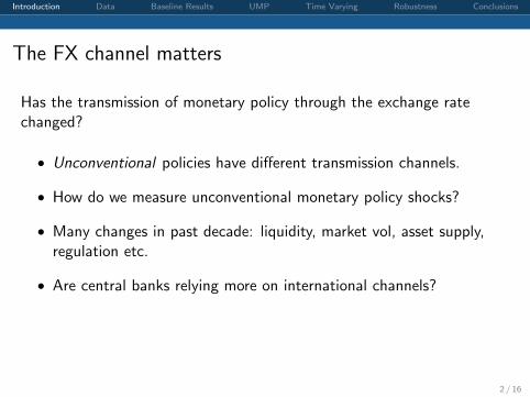
The FX channel matters
Has the transmission of monetary policy through the exchange ratechanged?
• Unconventional policies have different transmission channels.
• How do we measure unconventional monetary policy shocks?
• Many changes in past decade: liquidity, market vol, asset supply,regulation etc.
• Are central banks relying more on international channels?
2 / 16

Introduction Data Baseline Results UMP Time Varying Robustness Conclusions
The FX channel matters
Has the transmission of monetary policy through the exchange ratechanged?
• Unconventional policies have different transmission channels.
• How do we measure unconventional monetary policy shocks?
• Many changes in past decade: liquidity, market vol, asset supply,regulation etc.
• Are central banks relying more on international channels?
2 / 16
Introduction Data Baseline Results UMP Time Varying Robustness Conclusions
Methodology
What is the FX respose to a monetary policy announcement?
We use a high-frequency event study:
• Abstracts from endogeneity.
• Isolates impact from other news in either country during the day.
• Enables estimation of time-varying sensitivity.
• Enables estimation of the impact of different types of news.
• Well established technique: eg Faust et al 2003, Kearns & Manners2006, Rosa 2011, Glick & Leduc 2013, Gurkaynak & Wright 2013,Rogers et al 2014, etc
3 / 16

Introduction Data Baseline Results UMP Time Varying Robustness Conclusions
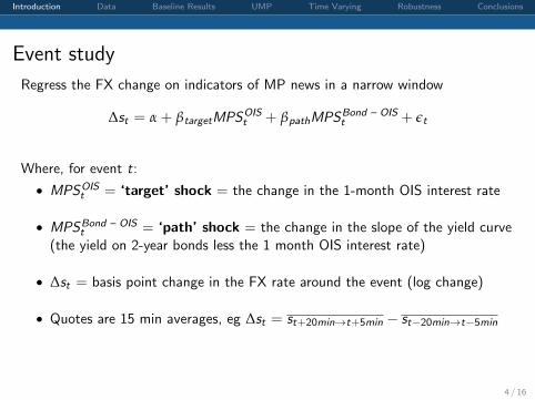
Event study
Regress the FX change on indicators of MP news in a narrow window
∆st = α + βtargetMPSOISt + βpathMPSBond – OIS
t + εt
Where, for event t:
• MPSOISt = ‘target’ shock = the change in the 1-month OIS interest rate
• MPSBond – OISt = ‘path’ shock = the change in the slope of the yield curve
(the yield on 2-year bonds less the 1 month OIS interest rate)
• ∆st = basis point change in the FX rate around the event (log change)
• Quotes are 15 min averages, eg ∆st = st+20min→t+5min − st−20min→t−5min
4 / 16
Introduction Data Baseline Results UMP Time Varying Robustness Conclusions
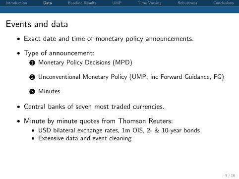
Events and data
• Exact date and time of monetary policy announcements.
• Type of announcement:
1 Monetary Policy Decisions (MPD)
2 Unconventional Monetary Policy (UMP; inc Forward Guidance, FG)
3 Minutes
• Central banks of seven most traded currencies.
• Minute by minute quotes from Thomson Reuters:• USD bilateral exchange rates, 1m OIS, 2- & 10-year bonds• Extensive data and event cleaning
5 / 16
Introduction Data Baseline Results UMP Time Varying Robustness Conclusions
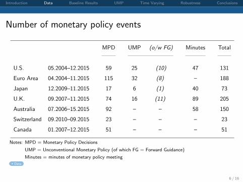
Number of monetary policy events
MPD UMP (o/w FG) Minutes Total
U.S. 05.2004–12.2015 59 25 (10) 47 131
Euro Area 04.2004–11.2015 115 32 (8) – 188
Japan 12.2009–11.2015 17 6 (1) 40 73
U.K. 09.2007–11.2015 74 16 (11) 89 205
Australia 07.2006–15.2015 92 – – 58 150
Switzerland 09.2010–09.2015 23 – – – 23
Canada 01.2007–12.2015 51 – – – 51
Notes: MPD = Monetary Policy Decisions
UMP = Unconventional Monetary Policy (of which FG = Forward Guidance)
Minutes = minutes of monetary policy meeting
Data
6 / 16
Introduction Data Baseline Results UMP Time Varying Robustness Conclusions
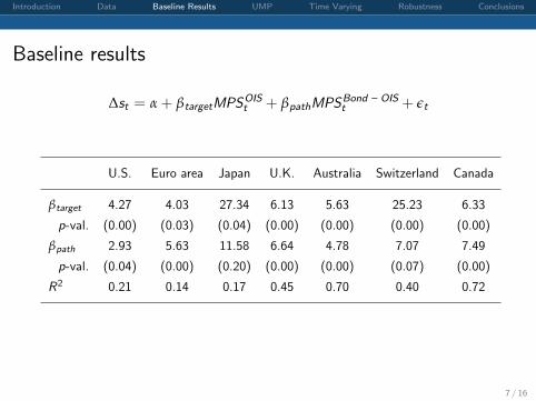
Baseline results
∆st = α + βtargetMPSOISt + βpathMPSBond – OIS
t + εt
U.S. Euro area Japan U.K. Australia Switzerland Canada
βtarget 4.27 4.03 27.34 6.13 5.63 25.23 6.33
p-val. (0.00) (0.03) (0.04) (0.00) (0.00) (0.00) (0.00)
βpath 2.93 5.63 11.58 6.64 4.78 7.07 7.49
p-val. (0.04) (0.00) (0.20) (0.00) (0.00) (0.07) (0.00)
R2 0.21 0.14 0.17 0.45 0.70 0.40 0.72
7 / 16
Introduction Data Baseline Results UMP Time Varying Robustness Conclusions
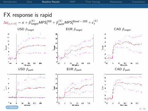
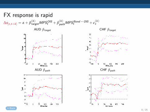
FX response is rapid∆s[t,t+k ] = α + β
(k)targetMPSOIS
t + β(k)pathMPSBond – OIS
t + ε(k)t
USD βtarget
USD βpath
EUR βtarget
EUR βpath
CAD βtarget
CAD βpath
Others8 / 16
Introduction Data Baseline Results UMP Time Varying Robustness Conclusions
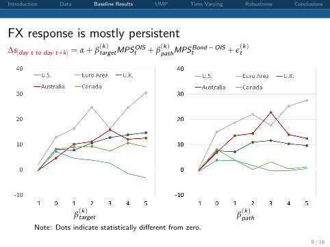
FX response is mostly persistent∆s[day t to day t+k] = α + β
(k)targetMPSOIS
t + β(k)pathMPSBond – OIS
t + ε(k)t
β(k)target β
(k)path
Note: Dots indicate statistically different from zero.
9 / 16

Introduction Data Baseline Results UMP Time Varying Robustness Conclusions
UMP events don’t seem that different
∆st = α + (βtarget + βUMPtarget1
UMP)MPSOISt
+(βpath + βUMPpath 1
UMP)MPSBond - OISt + εt
U.S. Euro Area U.K.
βtarget 3.19 4.57 6.91
p-val. (0.00) (0.10) (0.00)
βpath 1.63 6.56 8.29
p-val. (0.01) (0.02) (0.00)
βUMPtarget 9.76 0.46 -0.35
p-val. (0.22) (0.96) (0.87)
βUMPpath 10.92 -1.95 -0.97
p-val. (0.00) (0.61) (0.76)
R2 0.52 0.22 0.51
Others
10 / 16

Introduction Data Baseline Results UMP Time Varying Robustness Conclusions
UMP events don’t seem that different
∆st = α + (βtarget + βUMPtarget1
UMP)MPSOISt
+(βpath + βUMPpath 1
UMP)MPSBond - OISt + εt
U.S. Euro Area U.K.
βtarget 3.19 4.57 6.91
p-val. (0.00) (0.10) (0.00)
βpath 1.63 6.56 8.29
p-val. (0.01) (0.02) (0.00)
βUMPtarget 9.76 0.46 -0.35
p-val. (0.22) (0.96) (0.87)
βUMPpath 10.92 -1.95 -0.97
p-val. (0.00) (0.61) (0.76)
R2 0.52 0.22 0.51
Others10 / 16
Introduction Data Baseline Results UMP Time Varying Robustness Conclusions
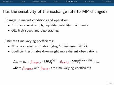
Has the sensitivity of the exchange rate to MP changed?
Changes in market conditions and operation:
• ZLB, safe asset supply, liquidity, volatility, risk premia.
• QE, high-speed and algo trading.
Estimate time-varying coefficients:
• Non-parametric estimation (Ang & Kristensen 2012).
• Coefficient estimates downweight more distant observations.
∆st = αt + βtarget,t ·MPSOISt + βpath,t ·MPSBond – OIS
t + εt ,
where βtarget,t and βpath,t are time-varying coefficients
11 / 16
Introduction Data Baseline Results UMP Time Varying Robustness Conclusions
Has the sensitivity of the exchange rate to MP changed?
Changes in market conditions and operation:
• ZLB, safe asset supply, liquidity, volatility, risk premia.
• QE, high-speed and algo trading.
Estimate time-varying coefficients:
• Non-parametric estimation (Ang & Kristensen 2012).
• Coefficient estimates downweight more distant observations.
∆st = αt + βtarget,t ·MPSOISt + βpath,t ·MPSBond – OIS
t + εt ,
where βtarget,t and βpath,t are time-varying coefficients
11 / 16

Introduction Data Baseline Results UMP Time Varying Robustness Conclusions
Time-varying coefficientsUSD βtarget
USD βpath
EUR βtarget
EUR βpath
12 / 16

Introduction Data Baseline Results UMP Time Varying Robustness Conclusions
Time-varying coefficientsGBP βtarget
GBP βpath
AUD βtarget
AUD βpath
CAD βtarget
CAD βpath
13 / 16

Introduction Data Baseline Results UMP Time Varying Robustness Conclusions
Why is monetary policy having a larger effect on FX?
Mostly it’s easier to rule out explanations.
• Not UMP:• Increase for Australia and Canada despite no/little UMP.
• UMP doesn’t have a larger impact in Europe or UK.
• The monotonic increase over the sample is inconsistent with:• FX risk premia – participants demand greater return for risk.
• Market liquidity – higher inventory risk when more news.
• Other possible explanations are harder to assess:• More information on long-run exchange rate in CB announcements.
• Changes in market structure – high-frequency and algorithmic trading.
• It could alternatively relate to the low level of interest rates.
14 / 16
Introduction Data Baseline Results UMP Time Varying Robustness Conclusions
Robustness
• Short rates have less explanatory power than long rates more
• Longer window to measure monetary shocks more
• 10-year bond (not 2-year bond) to measure path shocks more
• Define shocks as expectations and term-premium more
• Outliers – use M-estimator more
• Other bilateral FX or index for US; EUR/CHF for Switzerland more
• Release of policy committee meeting minutes more
• Rolling window OLS with just 2-year bond to measure MPS more
• Time-varying response to macro data releases more
15 / 16
Introduction Data Baseline Results UMP Time Varying Robustness Conclusions
Conclusions
1 Monetary policy continues to have a significant effect on exchangerates.
• Long interest rates are important for FX response.
• Common framework using short and long rates can characteriseMP shocks before and at ZLB.
• Effect of UMP is mostly similar to conventional MP.
2 The impact of monetary policy on the exchange rate has increasedover time.
• Not driven by UMP.
• Increase is broadly monotonic – doesn’t align with changes inliquidity, risk premia etc. changes in market conditions.
16 / 16

Extra slides
1 / 25

Magnitude of market responses around MP eventsAbsolute average changes in basis points
Policy Rate Target Path ∆y (2) ∆y(10)⊥ FX Spot
U.S. 7.8 1.0 2.2 1.7 1.8 17.4
Euro Area 5.5 0.9 1.1 0.8 0.7 12.6
Japan 0.0 0.2 0.3 0.3 0.9 10.3
U.K. 4.9 1.4 2.1 1.6 0.9 16.5
Australia 9.5 2.9 2.8 2.6 0.8 21.8
Switzerland 6.3 0.6 1.2 1.0 0.5 29.1
Canada 7.9 1.9 3.1 2.6 0.8 31.9
Notes: Target = ∆ 1-month OIS; Path = ∆(2-year bonds minus 1-month OIS).
∆y(10)⊥ is the change in the 10-year bond yield orthogonal to that in the 2-year bond yield.
Go Back
2 / 25

Interest rate variation around announcementsAbsolute average change over all announcements
1-month OIS 2-year yield
Go Back
3 / 25
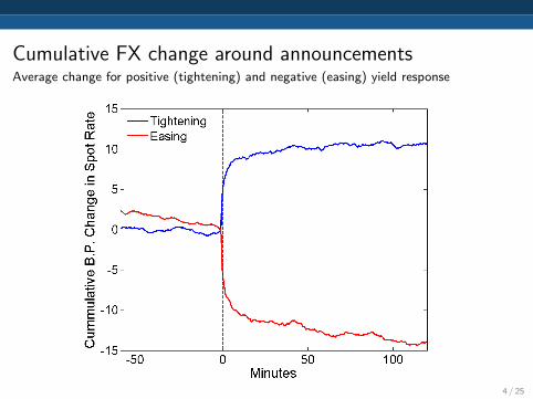
Cumulative FX change around announcementsAverage change for positive (tightening) and negative (easing) yield response
Go Back
4 / 25

Robustness: Expectation and Term Premium shocks
∆st = α + βexpMPS2yt + βtpMPS10y⊥
t + εt
Where:
• MPS2yt = ‘expectations’ shock = the change in the 2-year bond yield
• MPS10y⊥t = ‘term premium’ shock = orthogonal component of changes in
the 10-year bond yield
5 / 25

Robustness: Expectation and Term Premium shocks
∆st = α + βexpMPS2yt + βtpMPS10y⊥
t + εt
U.S. Euro area Japan U.K. Australia Switzerland Canada
βexp 3.07 4.66 1.21 3.94 5.41 11.31 7.09
p-val. (0.00) (0.00) (0.38) (0.00) (0.00) (0.00) (0.00)
βtp 2.65 8.23 -0.10 4.12 4.56 24.33 -0.89
p-val. (0.00) (0.00) (0.87) (0.04) (0.00) (0.00) (0.73)
R2 0.36 0.35 0.00 0.45 0.68 0.39 0.67
6 / 25

FX response is rapid∆s[t,t+k ] = α + β
(k)targetMPSOIS
t + β(k)pathMPSBond – OIS
t + ε(k)t
JPY βtarget
JPY βpath
GBP βtarget
GBP βpath
Back7 / 25
FX response is rapid∆s[t,t+k ] = α + β
(k)targetMPSOIS
t + β(k)pathMPSBond – OIS
t + ε(k)t
AUD βtarget
AUD βpath
CHF βtarget
CHF βpath
Back8 / 25
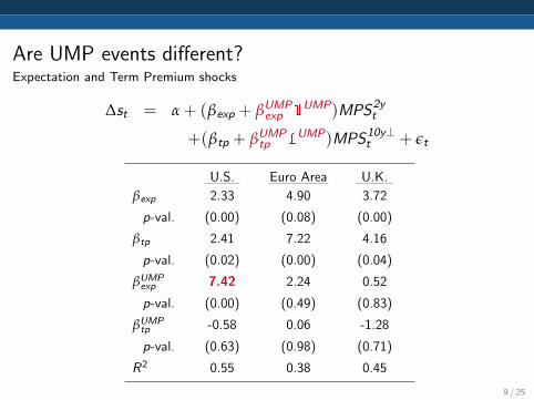
Are UMP events different?Expectation and Term Premium shocks
∆st = α + (βexp + βUMPexp 1
UMP)MPS2yt
+(βtp + βUMPtp 1
UMP)MPS10y⊥t + εt
U.S. Euro Area U.K.
βexp 2.33 4.90 3.72
p-val. (0.00) (0.08) (0.00)
βtp 2.41 7.22 4.16
p-val. (0.02) (0.00) (0.04)
βUMPexp 7.42 2.24 0.52
p-val. (0.00) (0.49) (0.83)
βUMPtp -0.58 0.06 -1.28
p-val. (0.63) (0.98) (0.71)
R2 0.55 0.38 0.45
Back
9 / 25
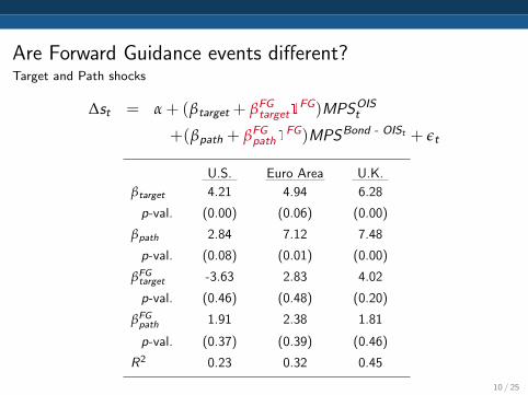
Are Forward Guidance events different?Target and Path shocks
∆st = α + (βtarget + βFGtarget1
FG)MPSOISt
+(βpath + βFGpath1
FG)MPSBond - OISt + εt
U.S. Euro Area U.K.
βtarget 4.21 4.94 6.28
p-val. (0.00) (0.06) (0.00)
βpath 2.84 7.12 7.48
p-val. (0.08) (0.01) (0.00)
βFGtarget -3.63 2.83 4.02
p-val. (0.46) (0.48) (0.20)
βFGpath 1.91 2.38 1.81
p-val. (0.37) (0.39) (0.46)
R2 0.23 0.32 0.45
Back
10 / 25

Are Forward Guidance events different?Expectation and Term Premium shocks
∆st = α + (βexp + βFGexp1
FG)MPS2yt
+(βtp + βFGtp 1
FG)MPS10y⊥t + εt
U.S. Euro Area U.K.
βexp 2.88 5.35 3.62
p-val. (0.00) (0.05) (0.00)
βtp 3.59 7.47 4.01
p-val. (0.00) (0.00) (0.03)
βFGexp 6.29 4.86 4.07
p-val. (0.09) (0.08) (0.06)
βFGtp 3.36 3.50 3.15
p-val. (0.54) (0.51) (0.44)
R2 0.54 0.40 0.37
Back
11 / 25

Spillovers
• Interest rate changes in large countries (eg US) may affect other countries’ rates.
• The FX response then reflects both interest rate changes.
• To check the importance of spillovers we estimate with GMM the system ofequations:
MPS jc,t = δMPS j
m,t + ε1c,t (1)
∆scm,t = α + β1MPS jm,t + β2MPS j
c,t + ε2cm,t (2)
• We find spillovers a very small within our narrow window.
12 / 25

Robustness: Univariate regression results
OIS 1-Month OIS 6-Months 2-Year Bonds 10-Year Bonds
U.S. β 2.36 4.20 3.07 3.26
P-value (0.00) (0.00) (0.01) (0.00)
R2 0.04 0.10 0.19 0.30
Euro area β -0.04 0.04 4.67 8.74
P-value (0.62) (0.93) (0.01) (0.00)
R2 0.00 0.00 0.11 0.35
Japan β 15.27 -0.33 1.21 0.16
P-value (0.18) (0.83) (0.42) (0.60)
R2 0.15 0.00 0.00 0.00
Go Back
13 / 25

Robustness: Univariate regression results
OIS 1-Month OIS 6-Months 2-Year Bonds 10-Year Bonds
U.K. β 0.57 1.15 3.95 5.38
P-value (0.00) (0.03) (0.01) (0.00)
R2 0.02 0.03 0.29 0.41
Australia β 3.62 3.47 5.41 11.25
P-value (0.00) (0.00) (0.00) (0.00)
R2 0.38 0.50 0.65 0.57
Switzerland β 2.39 4.67 11.31 23.68
P-value (0.09) (0.05) (0.00) (0.00)
R2 0.04 0.07 0.26 0.38
Canada β 2.66 6.35 7.09 13.10
P-value (0.10) (0.00) (0.00) (0.00)
R2 0.08 0.48 0.68 0.39
Go Back
14 / 25
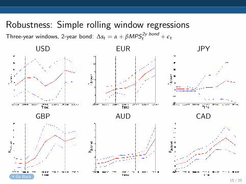
Robustness: Simple rolling window regressionsThree-year windows, 2-year bond: ∆st = α + βMPS2y bond
t + εt
USD
GBP
EUR
AUD
JPY
CAD
Go Back15 / 25
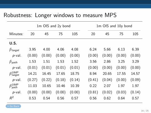
Robustness: Longer windows to measure MPS
1m OIS and 2y bond 1m OIS and 10y bond
Minutes: 20 45 75 105 20 45 75 105
U.S.
βtarget 3.95 4.00 4.06 4.08 6.24 5.66 6.13 6.39
p-val. (0.00) (0.00) (0.00) (0.00) (0.00) (0.00) (0.00) (0.00)
βpath 1.53 1.51 1.53 1.52 3.56 2.86 3.25 3.29
p-val. (0.01) (0.01) (0.01) (0.01) (0.00) (0.00) (0.00) (0.00)
βUMPtarget 14.21 16.45 17.65 18.75 8.94 20.65 17.55 14.57
p-val. (0.27) (0.22) (0.18) (0.14) (0.41) (0.04) (0.00) (0.09)
βUMPpath 11.03 10.65 10.46 10.39 0.22 2.07 1.97 1.97
p-val. (0.00) (0.00) (0.00) (0.00) (0.81) (0.02) (0.03) (0.14)
R2 0.53 0.54 0.56 0.57 0.56 0.62 0.64 0.57
Go Back
16 / 25
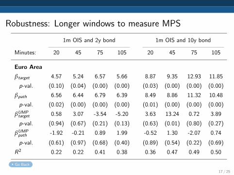
Robustness: Longer windows to measure MPS
1m OIS and 2y bond 1m OIS and 10y bond
Minutes: 20 45 75 105 20 45 75 105
Euro Area
βtarget 4.57 5.24 6.57 5.66 8.87 9.35 12.93 11.85
p-val. (0.10) (0.04) (0.00) (0.00) (0.03) (0.00) (0.00) (0.00)
βpath 6.56 6.44 6.79 6.39 8.49 8.86 11.32 10.48
p-val. (0.02) (0.00) (0.00) (0.00) (0.01) (0.00) (0.00) (0.00)
βUMPtarget 0.58 3.07 -3.54 -5.20 3.63 13.24 0.72 3.89
p-val. (0.94) (0.67) (0.21) (0.13) (0.63) (0.01) (0.80) (0.27)
βUMPpath -1.92 -0.21 0.89 1.99 -0.52 1.30 -2.07 0.74
p-val. (0.61) (0.97) (0.68) (0.40) (0.89) (0.54) (0.22) (0.69)
R2 0.22 0.22 0.41 0.38 0.36 0.47 0.49 0.50
Go Back
17 / 25

Robustness: Longer windows to measure MPS
1m OIS and 2y bond 1m OIS and 10y bond
Minutes: 20 45 75 105 20 45 75 105
U.K.
βtarget 6.91 4.66 3.44 2.69 4.75 4.15 3.76 2.71
p-val. (0.00) (0.00) (0.00) (0.04) (0.06) (0.07) (0.03) (0.12)
βpath 8.29 6.84 4.32 3.88 4.59 4.73 3.55 2.82
p-val. (0.00) (0.00) (0.01) (0.04) (0.09) (0.04) (0.05) (0.12)
βUMPtarget -0.35 -1.56 14.39 10.41 2.73 11.48 16.52 5.96
p-val. (0.87) (0.72) (0.07) (0.03) (0.34) (0.01) (0.04) (0.46)
βUMPpath -0.97 0.41 -0.50 3.07 -0.65 -0.33 -1.32 -1.18
p-val. (0.76) (0.89) (0.84) (0.22) (0.82) (0.89) (0.47) (0.52)
R2 0.51 0.35 0.20 0.14 0.42 0.42 0.21 0.11
Go Back
18 / 25
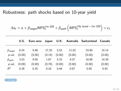
Robustness: path shocks based on 10-year yield
∆st = α + βtargetMPS1m OISt + βpath
(MPS10y bond – 1m OIS
t
)+ εt
U.S. Euro area Japan U.K. Australia Switzerland Canada
βtarget 6.24 9.48 17.20 5.53 11.02 33.90 14.14
p-val. (0.00) (0.00) (0.14) (0.00) (0.00) (0.00) (0.00)
βpath 3.53 9.00 1.67 5.23 9.27 16.98 14.39
p-val. (0.00) (0.00) (0.76) (0.00) (0.00) (0.00) (0.00)
R2 0.39 0.35 0.16 0.44 0.67 0.50 0.43
Go Back
19 / 25

Robustness: M-estimator to control for outliers
U.S. Euro area Japan U.K. Australia Switzerland Canada
OLS
βtarget 4.27 4.03 27.34 6.13 5.63 25.23 6.33
p-val. (0.00) (0.03) (0.04) (0.00) (0.00) (0.00) (0.00)
βpath 2.93 5.63 11.58 6.64 4.78 7.07 7.49
p-val. (0.04) (0.00) (0.20) (0.00) (0.00) (0.07) (0.00)
R2 0.21 0.14 0.17 0.45 0.70 0.40 0.72
M-estimator
βtarget 4.44 4.32 6.21 6.76 5.64 19.43 6.07
P-Value (0.00) (0.03) (0.32) (0.00) (0.00) ( 0.01) (0.00)
βpath 3.49 5.84 3.73 6.70 5.04 10.70 7.26
P-Value (0.00) (0.00) (0.51) (0.00) (0.00) ( 0.00) (0.00)
R2 0.21 0.14 0.04 0.45 0.70 0.36 0.72
Go Back20 / 25

Robustness: Other US dollar bilateral FX and index
EUR JPY U.K. AUD CHF CAD USD Index Long/Short
Target and path
βtarget 4.27 2.19 3.71 5.78 3.69 3.16 2.23 2.15
p-val. (0.00) (0.06) (0.00) (0.00) (0.00) (0.00) (0.06) (0.07)
βpath 2.93 2.98 2.22 2.72 3.35 1.60 2.97 3.00
p-val. (0.04) (0.05) (0.04) (0.10) (0.04) (0.07) (0.05) (0.04)
R2 0.21 0.24 0.22 0.15 0.24 0.26 0.24 0.24
Expectations and term premia
βexp 3.07 2.96 2.37 2.96 3.41 1.76 2.96 2.99
p-val. (0.00) (0.00) (0.00) (0.01) (0.00) (0.00) (0.00) (0.00)
βtp 2.65 3.08 2.09 2.72 2.45 1.55 3.06 3.10
p-val. (0.00) (0.00) (0.00) (0.00) (0.00) (0.00) (0.00) (0.00)
R2 0.36 0.55 0.37 0.22 0.39 0.20 0.55 0.54
Go Back21 / 25
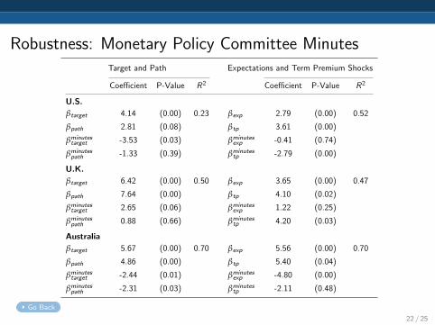
Robustness: Monetary Policy Committee MinutesTarget and Path Expectations and Term Premium Shocks
Coefficient P-Value R2 Coefficient P-Value R2
U.S.
βtarget 4.14 (0.00) 0.23 βexp 2.79 (0.00) 0.52
βpath 2.81 (0.08) βtp 3.61 (0.00)
βminutestarget -3.53 (0.03) βminutes
exp -0.41 (0.74)
βminutespath -1.33 (0.39) βminutes
tp -2.79 (0.00)
U.K.
βtarget 6.42 (0.00) 0.50 βexp 3.65 (0.00) 0.47
βpath 7.64 (0.00) βtp 4.10 (0.02)
βminutestarget 2.65 (0.06) βminutes
exp 1.22 (0.25)
βminutespath 0.88 (0.66) βminutes
tp 4.20 (0.03)
Australia
βtarget 5.67 (0.00) 0.70 βexp 5.56 (0.00) 0.70
βpath 4.86 (0.00) βtp 5.40 (0.04)
βminutestarget -2.44 (0.01) βminutes
exp -4.80 (0.00)
βminutespath -2.31 (0.03) βminutes
tp -2.11 (0.48)
Go Back
22 / 25

Robustness: FX response to data releases
∆st = α + βtargetnews shockOISt + βpathnews shock
Bond – OISt + εt
U.S. Euro area Japan U.K. Australia Switzerland Canada
βtarget 4.16 2.06 8.98 8.25 5.33 9.44 10.70
p-val. (0.00) (0.30) (0.09) (0.00) (0.00) (0.52) (0.00)
βpath 2.22 2.04 7.92 7.72 6.87 11.43 6.52
p-val. (0.00) (0.06) (0.14) (0.00) (0.00) (0.45) (0.00)
R2 0.17 0.03 0.28 0.40 0.77 0.00 0.40
Go Back
23 / 25

Robustness: FX response to data releases∆st = α + βtargetnews shock
OISt + βpathnews shock
Bond – OISt + εt
USD target
USD path
EUR target
EUR path
GBP target
GBP path
Go Back 24 / 25

Robustness: FX response to data releases∆st = α + βtargetnews shock
OISt + βpathnews shock
Bond – OISt + εt
AUD target
AUD path
CAD target
CAD path
Go Back 25 / 25