sectoral co-movement, monetary policy shocks, and input

Sectoral co-movement, monetary policy shocks, andinput- ow structure

Nao Sudou�

November 27, 2007

Abstract

Upon the monetary policy innovation, durable goods expenditure and non-durable expen-diture respond in the same direction.Conventional sticky price model, however, imply that they move to the opposite direction

(lack of co-movement), if either of the durable goods sector or non-durable sector sets theirprice in exible manner. In fact, many literatures assume that the durable goods prices are exible.If so, then the theory predicts that lack of co-movement is so severe, and the e�ect of

monetary policy is dampened nearly to the level of monetary neutrality (Barsky et al (2003,2007)).Our model o�ers one solution to this inconsistency. We depart from the prevalent as-

sumption that all the sectors face identical cost structure. In stead, we assume that eachsector obey the sector-speci�c cost structure that is consistent with input-output table.We �nd that even when the durable goods sector sets their price exibly, U.S. input-

output matrix may work so as to render the co-movement between the expenditures of thetwo products. The recovery of co-movenent brings back the monetary non-neutrality to theeconomy.

1 Introduction

Empirical literatures on price-setting behavior of �rms level have revealed that the stickiness ofprices are diverse across sectors (Bils and Klenow (2004), Nakamura and Steinsson (2006) for U.S.economy, and Dhyne et al (2006) and Alvarez and Luis (2006) for euro area countries). In otherwords, �rms that adjust prices once a month coexists with �rms that keep their prices �xed formore than a year. Moreover, the frequency of price change tends to di�er by sector. For example,the researches above commonly report that the price of service is adjusted less frequently than theprice of goods.On the other hand, the natural implication of this diversity, in conventional sticky price model

(ex. Calvo price model), is that the prices are adjusted at di�erent speed across sectors, after the

�Economist, Institute for Monetary and Economic Studies, Bank of Japan (E-mail: [email protected]) Theauthor would like to thank Robert King, Anton Braun, Simon Gilchrist, Francois Gourio, Adrian Verdelhan, NaohisaHirakata and the sta� of the Institute for Monetary and Economic Studies (IMES), the Bank of Japan, for theiruseful comments. Views expressed in this paper are those of the authors and do not necessarily re ect the o�cialviews of the Bank of Japan.

1

monetary policy innovation. Since the prices are adjusted di�erently across products, the relativeprices between them are temporary altered.Now, a question is what this relative price change brings about to the economy. The literatures,

including Ohanian et al (1995), Barsky et al (2003, 2006), Nakamura and Steinsson (2007), pointout that it leads to the acyclic response of sector that are exibly priced (lack of co-movement).In the wake of the monetary policy innovation, the relative price change incurs the substitutionacross the products by the households. When the size of the relative price change is signi�cantenough, the household reduces their spending on the relatively expensive products, even in theboom.

It is known that this lack of co-movement has the serious implication to the aggregate economy,when the durable goods is considered. Barsky et al (2003), Carlstrom and Fuerst (2006) 1 claim,from the theoretical point of view, that the lack of the co-movement between the durable goodssector and the non-durable sector should occur, because durable goods prices are exible whilenon-durable prices are sticky. In this speci�cation, the monetary expansion induces the decline indurable goods expenditure and the rise in non-durable expenditure. In terms of aggregate impact,the e�ect of the monetary policy shock is signi�cantly dampened, even to the level of monetaryneutrality.In contrast, the macro data indicates that the monetary policy shock induces the co-movement.

Figure 1 report the cumulative impulse response functions (CIRs) of the expenditures upon themonetary contraction shock. The CIRs are estimated from the VAR system employed similar tothe one in Erceg and Levin (2003). It is evident that both the durable goods expenditure and thenon-durable expenditure decline, and that the former declines more sharply.This co-movement observation from the data is consistent with the other empirical literatures.

Erceg and Levin (2002) shows that the disaggregated components of GDP decline upon the mone-tary contraction shock, and that of the non-durable GDP declines less. Barsky et al (2003) reportthat the durable goods production decline more sharply than the other sectors.Thus, we confront the con ict between the theoretical prediction and the empirical evidence.

Carlstrom and Fuerst (2006) names this inconsistency \co-movement puzzle."

The purpose of this paper is to o�er one way of solving this co-movement puzzle.Compared to the precedent researches, Barsky et al (2003, 2006) and Carlstrom and Fuerst

(2006), we focus on the production structure of each sector. Instead of assuming that all �rms inthe two sectors face identical cost structures, we assume that the cost structures of the �rms areconstructed so as to be consistent with input- ow matrix (or I-O matrix ) in U.S. economy. Hencethe cost structure of the �rms di�er by sector.Re ecting I-O matrix to our multi-sector model has the two advantages.First, I-O matrix provides the full description of inter-sectoral transaction by �rms. The use

of the matrix structure gives closer approximation of the actual �rms' cost minimization problem.Second, it is already known in the literature such as Horvath (1997), Dupor (1999) and Conley

and Dupor (2003), that the inter-sectoral transaction in the production process plays the signi�cantrole for sector-speci�c shock is transmitted to the other sectors. While they analyze the role ofI-O matrix structure in the context of the sector-speci�c productivity shocks and the propagationprocess, we concentrate on the analysis upon the sectoral responses and the propagation upon theaggregate demand shock. The analogical interpretation is possible because the response of thesectors to the monetary policy innovation are diverse, as the frequencies of the price adjustment

1See appendix for the categorization of durable goods and non-durables.

2

di�er by sector (Bils and Klenow (2004) and Nakamura and Steinsson (2006)). Just like theproductivity shock in the other sector is transmitted to own sector by input- ow relationship, thechange in the output of the other monopolistic producer a�ects the production of own sector bythe same relationship.

In the context of monetary policy analysis, this interaction across sectors is not fully examinedso far. In Bouakez et al (2005), only exception to our knowledge, the sectoral interaction iscaptured in terms of the demand-side dynamics. For example, the increase in the production ofthe sticky goods producing sector incurs the demands to the other sectors' product. The size ofthis inter-sectoral relationship is speci�ed by the I-O matrix. In contrast, our model highlightsto the inter-sectoral relationship in supply structure. As we see below, in current model, themost important channel is cost structure. The sectoral response of the material provider sectoristransmitted to the user sectors, and alters the response of aggregate economy.

This paper is organized as follows.Section 2 presents a set up of our model. We employ multi-sector sticky price model ( �M

sector model) where each sectors are heterogenous in the following three aspects : (1) degree ofnominal rigidity (frequency of price adjustment) dk; (2) cost structure represented by matrix, �and (3) durability of products. Note that our model only di�ers from Barsky et al (2003, 2007)and Carlstrom and Fuerst (2006) by the aspect (2) :Section 3 demonstrates the working mechanism. The distinct feature of our model appears in

price dynamics of the products. In our model, the prices of the each products are determined by (1)and (2) above, while only (1) is important in the economy where I-O matrix is abbreviated. Thepresence of aspect (2) alters the price dynamics of the products upon the monetary policy shock.Provided the prices across the products, households determine their expenditure decision over theproducts, referring to their relative prices. As Barsky (2003, 2007) emphasizes, the households'decisions are a�ected by durability � of the products.Section 4 is devoted for numerical exercises. We calculate the impulse response functions of

durable goods expenditure and non-durable expenditure, using reasonable parameter sets, andactual I-O matrix of the U.S. economy. In our model, whether the co-movement between durablegoods expenditure and non-durable expenditures obtained, depends on the structure of �; (2) :We �nd that the U.S. I-O matrix is consistent with the observed co-movement. We then considerthe two robustness tests for the co-movement results. One test checks the historical stability ofI-O matrix over the periods, since our result is dependent on the structure of the matrix. Oneother test checks the robustness of our result, when we modify the current two sector model tothe six sector model. We disaggregate the non-durable sector into subsectors, keeping durablegoods sector the same. This test is motivated by the current observation that the heterogeneity inprice stickiness in non-durable sector is large (Bils and Klenow(2004) and Nakamura and Steinsson(2006). We �nd the current model passes the two tests in terms of co-movement.Section 5 concludes.

2 The economy

2.1 Household

3

There is in�nitely-lived representative agent with preferences over consumption composite, Ct;

real money balance,Mt

Pt; and labor Lt, as described in expected utility function, (1). Labor is

completely mobile across sector.

U0 � E0

1Xt=0

�t�C1��t

1� �� '

L1+!

1 + !+ V

�Mt

Pt

��(1)

where � 2 (0; 1) is discount factor, � > 0 is the intertemporal elasticity of substitution, ! > 0is the inverse of the Frisch labor supply elasticity, and ' is the weight on leisure.Utility from real money balance is separable, where V is concave function of real money balance.

Ct is the aggregator, constructed from �M number of products produced in �M sectors, denoted as

C (m) ; for m = 1; ::: �M: Aggregator is expressed as follows, with weight m > 0;P �M

1 m = 1:

Ct =

�MYm=1

hC mt (m)

i(2)

The budget constraint for the households is:

�MXm=1

Pmt X

mt (m) +Mt � WtLt +

�MXm=1

�̂ (m) +Mt�1 + � t (3)

where Xt (m) is purchase of goods m;and Pmt is its price, Wt is nominal wage, �̂t (m) is the

pro�t from sectorm: Mt is nominal money stock, � t is a lump-sum nominal transfer from monetaryauthority.Law of motion for the stock of durable goods is described by the equations below. �m 2 [0; 1]

is the depreciation rate associated with the stock of goods m: Note that �m < 1 implies goods mis durable goods. For non-durables, Ct (m) = Xt (m) :

Ct (m) = (1� �m)Ct�1 (m) +Xt (m) (4)

2.2 Firm

The �rms in our model is similar to those in Huang et al (2004). We depart from their modelin a sense that we have multiple number of sectors present in the economy, and we abbreviatecapital, as being assumed in Basu (1995) and Long and Plossar (1993).Each sector, k; for 1; :: �M contains a large number of �rms j;each producing a di�erentiated

good, Xgt (j; k) ; indexed by j 2 [0; 1] : Superscript g stands for gross output. Denote a gross output

of composite of di�erentiated goods k; as Xgt (k) ; so that

Xgt (k) =

�Z 1

0

Xgt (j; k)

(��1)=� dj

��=(��1)where � 2 (1;1) are the elasticity of substitution between goods. The composite goods are

produced in an aggregation sector that is perfectly competitive. The price of composite goods k;denoted as P k

t (k) ; is related to the prices�P kt (j; k)

j2[0;1]of di�erentiated goods by

4

P kt (k) =

�Z 1

0

Pmt (j; k)

(1��) dj

�1=(1��)The gross output of composite good Xg

t (k) ; can serve as �nal consumption consumed by each i,

denoted as Xkt (k) =

R 10Xkt (i; k) di; and also as intermediate production input used by each �rm

j in each sector k, denoted as

�Xkt (k) =

�MXm=1

Z 1

0

�Xt (j; k;m) dj

where �Xt (j; k;m) denotes intermediate inputs of goods m used by the �rm j in sector k: Thegross output of �rm j in good k sector, denoted as Xg

t (j; k) ; requires intermediate productioninputs of �Xt (j; k;m) for m = 1; :: �M , labor L (j; k) ; with production function given by

Xgt (j; k) =

" �MYm=1

�Xt (j;m; k) (m;k)

#Lt (j; k)

(w;k) � Fc (5)

where (w; k) is labor share of sector k; which equals to 1�P �M

m=1 (m; k) ; and Fc is �xed costthat is identical across �rms (Huang et al (2004))2, and (m; k) 2 (0; 1) for m = 1; :: �M; whereP �M

m=1 (m; k) � 1 are the elasticity of output, with respect to the each of intermediate input,which equals to the factor share. In matrix form, we denote an input-use matrix for this economy,an �M � �M matrix, �;

� =

266664 11 12 : : : 1 �M�1 1 �M 21 : : : 2 �M: k;m k;k k;k+1 :: : : : :

�M1 �M2 : : : �M �M�1 �M �M

377775 (6)

where (m; k) indicates the factor share of commodity m; in producing commodity, k:In this set up, the cost minimization problem of �rm j; at sector, k; yields the marginal cost

function,

MCt (j; k) = ��W (w;k)t

�MYm=1

(Pmt )

(m;k) (7)

where �� is constant: Firms are price-takers in the inputs markets for input and monopolisticcompetitors in the products market. Nominal prices

�P kt (j; k)

j2[0;1] ; are chosen optimally in a

randomly staggered fashion, governed by the parameter dk 2 [0; 1); which is a probability that�rm in sector k; cannot adjust their price at a period (Calvo price setting). The �rm j in sector,k; then solves the following problem.

maxf �Xct (j;m;k) for m=1;::

�M; Lt(j;k);Pkt (j;k)gEt1Xs=0

(�dk)�t+s�t

Dt+s (j; k)

Pt+s(8)

2Huang et al (2004) set Fc so that there is no incentive to enter or exit for all sectors. This implies that steadystate pro�t of all sectors are zero. Our speci�cation for Fc is based on theirs.

5

s:t: Dt+s (j; k) = P kt (j; k)X

gt (j; k)�

�MXm=1

Pmt�X (j;m; k)�WtLt (j; k) (9)

where �t is Lagrange multiplier associated with budget constraint (3) :

2.3 Government

Monetary policy is conducted via lump-sum transfer so that

� t =Mt �Mt�1: (10)

2.4 Closing the Model

At the symmetric equilibrium, the market clear condition for good, k; is:

Xgt (k) =

�Z 1

0

Xgt (j; k)

(��1)=� dj

��=(��1)=

MXm=1

Z 1

0

�X (j;m; k) dj +X (k) for k = 1; ::M (11)

The �rst equality tells you that, the gross output of �rm j; in sector, k; are converted to thecomposite goods, Xg

t (k) : The gross output from the sector k; Xgt (k) is distributed to the �rms

and households. �X (j;m; k) is composite products, used by �rm j; in sector m; as intermediateinputs. X (k) is composite products k, consumed by household:Labor market is:

�MXm=1

Z 1

0

Lmt (j;m) dj = Lt (12)

where Lmt (j;m) is employment by �rm j in sector, m; at t:

2.5 Equilibrium

An equilibrium consists in a set of allocations, f Xgt (j;m) ; �Xt (j;m; k) ; Xt (i;m) ; P

mt (m) ; Wt;

Mt g1t=0; for all j 2 [0; 1] ; m; k = 1; ::: �M; that satis�es the following condition: (i) the household'sallocation solve its utility maximization problem, (ii) each producer's allocations and price solveits pro�t maximization problem taking the wage and all prices of intermediate goods. (iii) allmarkets clear.

6

3 Working mechanism

General discussionOur model di�ers from other multi-sector sticky price models, such as Ohanian et al (1995),

Barsky et al (2003, 2006), Carvalho (2006) and Nakamura and Steinsson (2007), by having I-Omatrix �: The important role of � is that it transmits the price dynamics of the material providerto its users. The channel is similar to the one discussed in Dupor (1999) and Horvath (1998),along the line of sector-speci�c shock.Upon the monetary policy shock, when the inter-sectoral relationship in the production process

is abbreviated, the price dynamics of each products re ects its own frequency of price adjustment,and labor (Carlstrom and Fuerst (2006)).When matrix I-O matrix � is explicitly considered, price dynamics of sectoral products re ect

dk of its intermediate inputs, as well as its own frequency of price adjustment. Therefore, as longas there is a link in intermediate inputs- ow, the price dynamics of the economy becomes distinct.For the households side, the price dynamics of each products ( and the products' depreciation

rate as we explain shortly) are the only issue taken into consideration, when they determine theirexpenditure plan over the products. Therefore, I-O matrix � a�ects the households' expenditures,by a�ecting relative price movement.

Firms' price setting decisionsWe start describing working forces of our model from price setting behavior of �rms, because it

splits our model from precedents. In short, we show that persistency of products is determined bytwo factors : (i) producers' own frequency of price adjustment, and (ii) stickiness of its intermediateinputs. Note that precedent literature stresses the role of (i) in the price dynamics upon themonetary policy shock, but not the role of (ii) :When a sector that sets the price exibly employ the products from the other sectors whose

prices are also exible, then its product prices do not demonstrate the persistency. On the otherhand, when exible sector import sticky products, its output inherits portion of stickiness origi-nated from the inputs.

In Calvo price setting framework we employ, newly set price at t, P �t (k; j) ; chosen by active �rmj; in sector k; satis�es the following relationship with the future nominal marginal cost mct+s (k) :

~p�t (k; j) = (1� dk�)Et

( 1Xs=0

(dk�)s (m~ct+s (k))

)(13)

where ~zt denotes the log-deviation of the variables Zt, and so ~p�t (k; j) and m~ct+s (k) are the

log-deviation of P �t (k; j) ; mct+s (k) ; respectively.Now nominal marginal cost for sector k, m~ct+s (k) is determined by,

m~ct+s (k) = (�k)T ~pt+s + (w; k) ~wt+s (14)

where �k is the kth column vector of I-O matrix �; T denotes transpose, and ~pt+s is columnvector whose m�th element is price deviation of products m at period t + s; ~pt+s (m) : Fromthe term (�k)

T ~pt+s; it is observable that the nominal marginal cost for sector k, m~ct+s (k) canbe expressed by the linear combination of prices of other sectors' product ~pt+s (m) : The relativesigni�cance of the speci�c sector in terms of prices may be measured by (m; k).

7

The two equations above (13) ; (14) indicate that the price dynamics of the product from sectork inherits price dynamics of product m: This is the case when sector k employes the product fromsector m as its intermediate inputs ( That is, (m; k) 6= 0). In view point of persistency of sectork, apart from the e�ect from dk; higher weight on sticky sectors as intermediate inputs bringsabout higher stickiness of price of products k. Hence even when product k is exibly priced, if �kcontains large nonzero element for some sticky sector, say h; then pt (k) may be more persistentthan the product of slightly sticky sector, depending on the size of (h; k) and stickiness of h:

Households' expenditure decisionFor the change of expenditures upon the monetary policy shock, the relative price and the

depreciation rate of the each products are responsible. Households decide their expenditure planover the set of products, m = 1; :: �M; referring to the relative prices movement across the products.When �m is smaller than 1, then the relative prices are not the only factor that determines thehouseholds' decision.The �rst order conditions of households' utility maximization problem yields following equa-

tions for non-durables m = m1;m2; (15) ; and for durable goods m = m3; (16) ; respectively. Notethat Xt (m3) 6= Ct (m3) for durables goods

3.

Ct (m1)��

Ct (m2)�� =

Pm1t

Pm2t

(15)

C1��t

Ct (m1)

Pm1t

Pm3t

= Et

" 1Xs=0

�s (1� �m3)s C1��t+s

Ct+s (m3)

#(16)

where Et denotes expectations, conditional on the information set available at time t.

As ((15)) indicates, when both products are non-durables, the consumption (expenditure)path for two products, Ct (m1) and Ct (m2) is direct re ection of the discrepancy in relative pricesbetween the two products. Higher relative price implies lower expenditure, and vice versa. Whetherthe expenditure of the product drops below the steady state is determined by the size of relativeprice change.

When the durable goods is considered, the expenditure pattern is a�ected by the intertemporalchoice ((16)) ; and the equation becomes more di�cult to interpret. There are two views onto howthe size of depreciation rate � a�ects the households' expenditure plan.Bils and Klenow (1998) points out that smaller depreciation rate implies that, a given change

in the durable goods consumption requires greater percentage in its expenditure. This claimapplies in the current model, since we assume that the consumption ow from the durable goodsis proportional to the stock (2). When the household reduces the consumption of durable goodsand non-durable by the same ratio, the expenditure on the durable goods tends to decline moreas � is smaller.For another view, Barsky et al (2003, 2007) claim that when short-lived shocks, like monetary

shocks, are considered, RHS of ((16)) may be approximated by constant. This is because marginal

3Our numerical exercise is conducted using Cobb-Douglas type of utility function. It is possible, however,

to assume that utility function has the shape such as Ct =P �M

m=1

h mCt (m)

��1�

i ��1

where � is elasticity of

substitution, instead of Cobb-Douglas. Carlstrom and Fuerst (2006) shows that the co-movement is only obtainedwhen � is unrealisically small.

8

utility is to short-lived shocks, when � is su�ciently small. If this argument holds true, the demandfor the durable goods displays an almost in�nite elasticity of intertemporal substitution (Barskyet al (2003,2007)), and the households' expenditure becomes sensitive to the price change. As aresult, a signi�cant decline in the relative price of the durable goods may lead to the increase inits expenditure, even during the monetary contraction.

We will see in the next section that, either Bils and Klenow (1994)s' view or Barsky et al (20032007)'s view may hold in the current model, depending on the size of relative price change incurredby monetary policy innovation. In monetary contraction, if the durable goods' prices are for anyreason low enough, the latter e�ect is dominant and the lack of co-movement is realized. Whenthe prices are low, the former channel becomes dominant and the co-movement is realized.

4 Co-movement across sectors

General discussionThis section conducts the numerical exercise. Our exercises follow the speci�cation of the

preceding researches by Barsky et al (2003, 2007) and Carlstrom and Fuerst (2006), other thanthe cost structure of the �rms. We show that using the information of I-O matrix of U.S. economy,co-movement puzzle is solved. Moreover, as a consequence of the co-movement between durablegoods expenditure and non-durable expenditure, money neutrality result obtained in Barsky et al(2003, 2007) are overturned.

As we will see, the co-movement result is brought about by the speci�c characteristic of U.S.I-O matrix structure. That is, the observation of U.S. I-O matrix indicates that the �rms in thedurable goods sector employ large amount of non-durables as intermediate inputs4. In other word,as we saw in (14) ; the marginal cost of durable goods production is signi�cantly a�ected by theprice dynamics of the non-durables. From (13) ; it is equivalent to saying that the prices of thedurable goods are a�ected by the price dynamics of the non-durables. Thus even when the prices ofdurable goods are adjusted exibly, price dynamics of the durable goods display some persistency.Since the households make their expenditure decisions by the relative price between durable goodsand non-durables ((16)) ; the co-movement in the expenditure is generated through this channel.

Throughout the numerical exercises, we consider that the monetary policy shock is a permanentdecrease of money supply by 1% at period t = 1. We consider an economy where steady statein ation rate is zero. We report the impulse response functions (IRFs) of the variables to themonetary policy innovation, and the summary table. The IRFs are calculated in terms of thedeviation from the steady state unless otherwise noted. The IRFs of the durable goods are depictedby the expenditure ow term.The exercise are conducted quarterly, following the treatment of the literatures that handles

I-O matrix, such as Horvath (2000), Bouakez et al (2003).The speci�cation of the model other than the production function of �rms are constructed so

that the implications are comparable to those of Barsky et al (2003,2006), Carlstrom and Fuerst(2006). See appendix for details.

4This characteristic of I-O matrix is also stressed in Hornstein and Praschnik (1997).

9

The lack of co-movement and co-movementWe start our numerical exercise by showing the lack of co-movement result. Figure 4a and

Figure 4b display the impulse response functions (IRFs) of the variables in the economy, wherethe production functions are linear with respect to the labor inputs. In both the durable goodssector and the non-durable sector, �rms produce their output independently.Figure 4a illustrates the lack of co-movement between the durable goods expenditure and

the non-durable expenditure. While the non-durable expenditure declines, the durable goodsexpenditure responds signi�cantly, but in the opposite direction.Figure 4b depicts the IRFs of aggregate variables (GDP5 and total labor supply). Note that

the response of the two variables are insigni�cant. As Barsky et al (2003, 2007) point out, sincethe expenditures on the two products change in the opposite direction, the impact of the monetarypolicy shock on the economy becomes negligibly small, in terms of the aggregate variables (moneyneutrality)

Next, we show the co-movement. We incorporate following 2� 2 matrix, � whose elements aretaken from the actual U.S. I-O matrix, of year 2005.

�2005�M=2 =

�.370 .278

.056 .279

�The �rst row indicates the share of non-durable inputs in the non-durable production (element

(1; 1)), and the share in the durable goods production (element (1; 2)); respectively. Similarly,the second row indicates the share of durable goods inputs in the non-durable production (element (2; 1)), and in the durable goods production (element (2; 2)); respectively.The noticeable feature from this matrix � is asymmetry in the intermediate inputs between non-

durable sector and durable goods sector. While the intermediate inputs in non-durable productionare mostly the products of its own sector, large portion of the intermediate inputs in durable goodsproduction is the products of the non-durable sector.In other word, this heterogeneity in the row sums between the two sectors indicates that the

non-durable sector is a relatively large material supplier to the economy than durable goods sector.From this point, it is predictable, from the corollary to the arguments made in Dupor (1999), thatsectoral response of the non-durable sector has a disproportionately larger e�ect on the aggregateeconomy.

Figure 4c and 4d show the IRFs of the variables in the economy where I-O matrix �2005�M=2is

incorporated. Both durable goods expenditure and non-durable expenditure decline upon themonetary contraction (Figure 4c). Thus the co-movement is recovered. It is also seen that thedecline of durable goods expenditure is larger than that of non-durables, as stressed by Bils andKlenow (1994).In terms of the aggregate variables, both GDP and labor supply declines signi�cantly, compared

to the IRFs displayed in Figure 4b. Thus money non-neutrality is recovered, too, even though wefollow the speci�cation of Barsky et al (2007) that the durable goods prices are exible.

Working mechanism

5We de�ne GDP as the weighted sum of the durable goods expenditure and the non-durable expenditure.Following Barsky et al (2003, 2007), the nominal expenditure share of each expenditure at the steady state is usedas the weight.

10

The working mechanism that yields the co-movement between the expenditures is generatedfrom the speci�c characteristic of I-O matrix. Especially, among the four elements of �2005�M=2

; thesize of (1; 2) plays the important role. Note that (1; 2) stands for the share of non-durableintermediate inputs in durable goods production.To see what separates the economy into the lack of co-movement and co-movement, and to

clarify the role of (1; 2), we calculate the IRFs of the variables using the di�erent �. In thisexercise, we keep both the production structure of the non-durable producing sector, and theshare of intermediate inputs in the durable goods producing sector ( (1; 2) + (2; 2)) unaltered.We alter the share of the non-durable inputs in the durable goods production, (1; 2) from .01 to.40, and depict the IRFs of the variables for each economy.

Figure 4e, f, g, h, i, j, k demonstrate the IRFs of the variables when the share of non-durable, (1; 2) rise from .01 to .40.Figure 4e indicates the response of nominal marginal cost in durable goods producing sector.

When non-durable share is small, the nominal marginal cost overshoots in the short run6. Thecost appears to be more persistent as (1; 2) rises. As shown in the equation (14) ; higher (1; 2)implies that the marginal cost of durable producing �rms are a�ected more, by the price dynamicsof non-durables. Since non-durable producing sector has sticky price, realized price of durablegoods price inherits some of that property, as (1; 2) increases. As a consequence, the relativeprice change between durable goods price and non-durable price shrink smaller (Figure 4f).Figure 4g and 4h show the expenditures of non-durables and durable goods for the di�erent

size of (1; 2).For the former, varying non-durable share does not seem to play the important role. Upon the

monetary contraction, it declines to around -.37 % from the steady state at the impact.For the latter, alteration in the size of (1; 2) induces change in both the sign and the size

of the IRF. When it is small, the durable goods expenditure rises more than 2% from the steadystate. This lack of co-movement observation is similar to the one reported in Barsky et al (2007).When (1; 2) becomes larger, the co-movement is recovered. The decline of the expenditure ismore than 1%, which is bigger than that of non-durables.

Figure 4i, 4j and 4k show the IRFs of the aggregate variables. It is noted that in our model,the short run dynamics of both total labor supply and the labor productivity are a�ected by thesize of (1; 2) 7: As the co-movement is recovered in the disaggregate components and the drop ofthe durable goods expenditure becomes bigger, both aggregate variables decline more prominently.The response of GDP departs from the money neutrality accordingly.

Table 2 summarizes the results. It reports the cumulative impulse response (CIR) of durablegoods expenditure and non-durable expenditure for the �rst two years after the monetary con-traction shock. The elements of each row are CIR of the variables for di�erent value of (1; 2):The co-movement is obtained only when (1; 2) is bigger than .20. The response of durable goodsexpenditure becomes greater than that of non-durable expenditure, only (1; 2) is larger than .25.

6The same phenomena is observed in Barsky et al (2003).7Labor productivity is de�ned as GDPtLt

: As Basu (1995) and Huang and Liu (2001) discuss, the monetary policyinnovation can induce the temporal change in the labor productivity, when the sticky intermediate goods price isincorporated. In the current exercises, both sticky intermediate goods price and exible intermediate goods priceare present. The rise of (1; 2) implies the rise in the share of the former. The change in the labor productivitybecomes prominent accordingly.

11

Combining those results imply that as (1; 2) rises, the view stressed by Bils and Klenow(1994) becomes more e�ective than the view stressed by Barsky et al (2003, 2007).

Sensitivity to the historical change in I-O matrixIn the following two subsections, we conduct two tests. The tests aim to check the robustness

of the co-movement result.First test asks if the property of U.S. I-O matrix that yields the co-movement between durable

goods expenditure and non-durable expenditure has been stable over time. We conduct this testby calculating IRFs of durable goods expenditure and non-durable expenditure using I-O matrixof the year that is di�erent from 2005. U.S. I-O matrix is constructed in every �ve years, we repeatthe same exercise we did in the previous section using the matrix constructed before 2005.Second test asks if the property of U.S. I-O matrix that yields the co-movement between

durable goods expenditure and non-durable expenditure has been robust when non-durable sectoris disaggregated into subsectors. The researches about the frequency of price adjustment reportthe heterogeneity in price stickiness across the subsectors of non-durable sector (Bils and Klenow(2004), Nakamura and Steinsson (2006)). We decompose the current non-durable sector into �vesubsectors and see whether the co-movement result is robust to this disaggregation.

For the �rst purpose, we calculate the elements of 2�2 matrix � again, using I-O table of U.S.economy from year 1963 to 2000. We then repeat the same numerical exercise as we did in thesubsections above, using newly obtained � of each year. We keep the other parameters, such asthe share of value added k; and the frequency of price adjustment dk; and the depreciation rate�; the same as the precedent exercises Especially, although the observed nominal share of valueadded of non-durable and durable goods are changing over this sample period, we concentrate onthe analysis of the change in I-O matrix �, and abbreviate the e�ect from the other parameters.Figure T-1 provides the calculated time-series of the four elements of I-O matrix � over the

sample periods. The �gures in each element are not completely constant, but huge uctuations arenot observed. Similar to the �gures of year 2005, the non-durable producing sector stays as thelarge material supplier to the durable goods producing sector during the period, though the share (1; 2) is to some extent, shifting around. The production structure of non-durable producing�rms are almost constant during the period.Figure T-2 and T-3 are IRFs of non-durable expenditure and durable goods expenditure to

the monetary contraction shock, respectively. Each lines are labelled by the year from which thematrix � is constructed.The responses of non-durable expenditure are always positive, and there is no signi�cant dif-

ference in the shape of IRFs across years. As for the responses of durable goods expenditure, onthe other hand, there is a signi�cant variation in the shape of IRFs across years. Especially, forthe year 1963 and 1972, where the �gure of (1; 2) is comparatively smaller than the other years,the response of durable goods expenditure is modest.From the comparison between Figure T-2 and Figure T-3, it is observable that the property

that durable goods expenditure respond more than does non-durable expenditure is not obtainedfor year 1963 and 1972. For other years, durable goods expenditure responds more than does non-durables. The co-movement between the durable goods expenditure and non-durable expenditure,however, are robust throughout the sample period, including year 1963 and 1972.

Sensitivity to categorizationIn the second test, we divide non-durable sectors into several subsectors. We disaggregate the

12

I-O matrix, too. The criteria of this disaggregation process is the reported frequency of pricechange dk.While \non-durable", in our terminology, include the broad category of products that may be

di�er in price stickiness dk, the current two-sector model treats those products as having the samedegree of price stickiness. However, recent empirical observation conducted by Bils and Klenow(2004) and Nakamura and Steinsson (2006) reveal that the frequency of price adjustment is diverseacross subsectors of \non-durable" sector. For example, prices of utilities, travel and unprocessedfood are said to be comparatively exible.Note that the e�ectiveness of current model as a solution to the co-movement puzzle relies

on the frequency of price adjustment dk of speci�c intermediate inputs that are used in durablegoods production. For instance, when the subset of non-durables inputs supplied to durable goodsproducing �rms happen to be those whose prices are relatively exible among non-durables, thenthe channel argued so far may not be operative.

In order to test the robustness of co-movement result, we decompose non-durable sector intofour subsectors and the rest (Five sectors for total). The rules of the decomposition are service-and-non-durable goods distinction, and the observed di�erence in the frequency of price adjustment.Among the products of service, we extract utilities and transportation for their reported frequencyof price adjustment is high (Nakamura and Steinsson (2006)). We extract food from non-durablegoods by the same reason. This procedure extends the number of sectors to six.With renewed those �ve sectors, we calculate � �M=6 again, and conduct calibration.

Figure T-5, displays the IRFs of the non-durable expenditure and durable goods expenditure,generated from the same six sector model. In this experiment, � is neglected and linear productionwith respect to labor inputs are assumed for each sector. The frequencies of price adjustment foreach sector dk are the same as those used in the experiment displayed in Figure T-6. Apparentlythe co-movement is not obtained.

Figure T-4 shows the IRFs of non-durables expenditure and durable goods expenditure inmonetary contraction, in six sector economy. 6�6 I-O matrix � is constructed from U.S. I-O tableof year 2005. Note that in this economy, non-durable expenditure is the sum of the �ve di�erentproducts (other service, food, other non-durable goods, utility and transportation), produced fromthe �ve di�erent sectors. For each sector, the frequency of price adjustment is speci�ed accordingto the micro-level �nding of Bils and Klenow (2004).This six sector model should capture the impact of the heterogeneity within the subsectors of

broad \non-durable" sector. It is seen from the �gure T-4 that the co-movement between aggregatenon-durable expenditure and durable goods expenditure is obtained in this speci�cation, too.Moreover, the durable goods expenditure declines more than that of non-durable expenditure asobserved in the Table 1. Thus co-movement results is robust to the disaggregation of non-durablesector at least into �ve sectors.

5 Conclusion

In the current paper, we o�er one solution to the co-movement puzzle proposed by Barsky etal (2003) and Carlstrom and Fuerst (2006).

13

The co-movement between non-durables expenditure and durable goods' expenditure uponmonetary policy innovation may be generated through I-O matrix, in the case where non-durableprices are sticky and durable goods prices are exible. As a consequence of recovery of the co-movement, money non-neutrality is obtained within the framework where durable goods price arecompletely exible. This results contrasts with the results in Barsky et al (2007).Our outcome is generated from the speci�c characteristic of U.S. input-output structure. In

U.S. I-O matrix, non-durable producing sector serves as disproportionately large material supplierto durable goods sector. Thus price dynamics of durable goods is a�ected by the price dynamicsof non-durables. We showed that this inter-sectoral relationship between the sectors preventsthe drastic departure of relative prices across the products. Since the relative price change ismitigated, the households' expenditure over the two products respond to the same direction, uponthe monetary policy shock (co-movement).In order to check the robustness, two sensitive tests are conducted. We con�rm that U.S.

I-O matrix keeps the speci�c structure that yields the co-movement over long period time. Wealso con�rm that U.S. I-O matrix keeps the structure that yields the co-movement even whennon-durable sector is disaggregated into several subsectors.

6 Appendix 1 parameters

Parameters are chosen, following Carlstrom and Fuerst (2006).Baseline parameters

Parameter Value Description

� (1:04)�1 Yearly subjective discount rate� 2 Intertemporal elasticity of substitution� 1 Elasticity of substitution!�1 1 Frisch labor supply elasticity�k = � 11 Elasticity of substitution across goods� 10% Annual depreciation rate of durable goods

7 Appendix 2 sector speci�c parameters

This section explains the estimating methodology and the source of sector speci�c parameters em-

ployed in our calculation. The parameters are input share �; value-added share k and the frequency ofprice adjustment dk:

Our calibration contains two sector, six sector level of disaggregation. �; k for each sector areconstructed from U.S. use matrix of corresponding year. As for dk; we refer both Bils and Klenow (2004),Nakamura and Steinsson (2006) and the arguments in Barsky et al (2003).

.

CategorizationCalculation of � and k is the matter of categorization. The current paper concentrates the analysis

on the two sectors, durable goods sector and non-durable sector. Our durable goods categorization

is constructed so as to be consistent with the preceding two sector models that explicitly incorporate

14

the durable goods sector (Barsky et al (2003, 2007), Carlstrom and Fuerst (2006) and Baxter (1996)

and Hornstein and Praschnik (1997)). That is, durable goods expenditure includes consumer durable

expenditure and investment. This categorization di�ers from Erceg and Levin (2003).

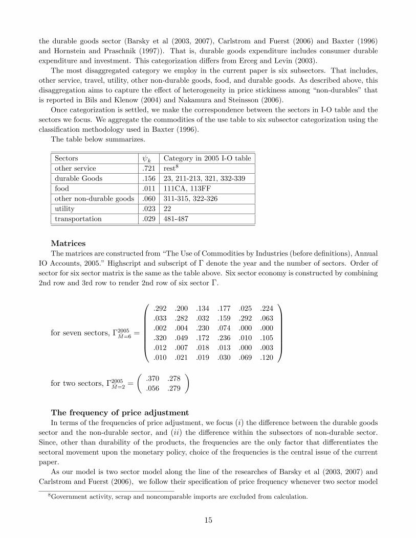
The most disaggregated category we employ in the current paper is six subsectors. That includes,

other service, travel, utility, other non-durable goods, food, and durable goods. As described above, this

disaggregation aims to capture the e�ect of heterogeneity in price stickiness among \non-durables" that

is reported in Bils and Klenow (2004) and Nakamura and Steinsson (2006).

Once categorization is settled, we make the correspondence between the sectors in I-O table and the

sectors we focus. We aggregate the commodities of the use table to six subsector categorization using the

classi�cation methodology used in Baxter (1996).

The table below summarizes.

Sectors k Category in 2005 I-O table

other service .721 rest8

durable Goods .156 23, 211-213, 321, 332-339

food .011 111CA, 113FF

other non-durable goods .060 311-315, 322-326

utility .023 22

transportation .029 481-487

MatricesThe matrices are constructed from \The Use of Commodities by Industries (before de�nitions), Annual

IO Accounts, 2005." Highscript and subscript of � denote the year and the number of sectors. Order ofsector for six sector matrix is the same as the table above. Six sector economy is constructed by combining

2nd row and 3rd row to render 2nd row of six sector �:

for seven sectors, �2005�M=6=

[email protected] .200 .134 .177 .025 .224

.033 .282 .032 .159 .292 .063

.002 .004 .230 .074 .000 .000

.320 .049 .172 .236 .010 .105

.012 .007 .018 .013 .000 .003

.010 .021 .019 .030 .069 .120

1CCCCCCAfor two sectors, �2005�M=2

=

�.370 .278

.056 .279

�

The frequency of price adjustmentIn terms of the frequencies of price adjustment, we focus (i) the di�erence between the durable goods

sector and the non-durable sector, and (ii) the di�erence within the subsectors of non-durable sector.Since, other than durability of the products, the frequencies are the only factor that di�erentiates the

sectoral movement upon the monetary policy, choice of the frequencies is the central issue of the current

paper.

As our model is two sector model along the line of the researches of Barsky et al (2003, 2007) and

Carlstrom and Fuerst (2006), we follow their speci�cation of price frequency whenever two sector model

8Government activity, scrap and noncomparable imports are excluded from calculation.

15

is concerned. Thus our two sector model assumes quarterly frequency of price adjustment dk = 0 fordurable goods sector and dk = :67 for non-durable sector, that are the setting of Carlstrom and Fuerst

(2006).

In the six sector analysis in section 4, we employ the �ndings from micro data (Bils and Klenow

(2004) and Nakamura and Steinsson (2006)), rather than the values of Carlstrom and Fuerst (2006).

Since the motivation of six sector analysis itself is to check the implication of the observed heterogeneity

in price stickiness in non-durable sector, our speci�cation re ects the �gures from the micro data. dkfor subsectors of non-durable, travel, utility and food are taken from Nakamura and Steinsson (2006).

dk for service less travel, and non-durable goods less food are chosen, so that the mean of the frequencyof service and non-durable goods, weighted by the relative signi�cance of each items in value-added of

year 2005, to be equalized to the �gure of service and non-durable goods, reported in Bils and Klenow

(2004).

References

[1] Alvarez, Luis J. (2006) : \Sticky Prices in the Euro Area: A Summary of NewMicro-evidence,"Journal of the European Economic Association, v. 4, iss. 2-3, pp. 575-84

[2] Bak, Peter, Chen, Kan, Scheinkman, Jose and Woodford, Michael (1992) : \Aggregate Fluc-tuations from Independent Sectoral Shocks: Self-Organized Criticality in a Model of Produc-tion and Inventory Dynamics," National Bureau of Economic Research, Inc, NBER WorkingPapers: 4241

[3] Barsky, Robert, Christopher L. House, Miles Kimball (2003) : \Do Flexible Durable GoodsPrices Undermine Sticky Price Models?," National Bureau of Economic Research, Inc, NBERWorking Papers: 9832.

[4] Barsky, Robert, Christopher L. House, Miles Kimball (2007) : \Sticky Price Models andDurable Goods," American Economic Review, 97(3).

[5] Basu, Susanto (1995) : \Intermediate Goods and Business Cycles: Implications for Produc-tivity and Welfare," American Economic Review, 85(3).

[6] Baxter, Marianne (1996) : \Are Consumer Durables Important for Business Cycles?" Reviewof Economics and Statistics, 78(1).

[7] Bernanke, Ben S., Boivin, Jean; Eliasz, Piotr (2005) : \Measuring the E�ects of MonetaryPolicy: A Factor-Augmented Vector Autoregressive (FAVAR) Approach," Quarterly Journalof Economics, 120(1).

[8] Bils,Mark;Klenow,PeterJ (1998) : \Using Consumer Theory to Test Competing BusinessCycle Models," Journal of Political Economy, 106(2).

[9] Bils, Mark, Klenow, Peter J. and Kryvtsov, Oleksiy (2003) : \Sticky Prices and MonetaryPolicy Shocks," Federal Reserve Bank of Minneapolis Quarterly Review, 27(1).

[10] Bils, Mark, Peter J. Klenow (2004) : \Some Evidence on the Importance of Sticky Prices,"Journal of Political Economy, 112(5).

16

[11] Boivin, Jean, Giannoni, Marc and Mihov, Ilian (2007) : \Sticky Prices and Monetary Policy:Evidence from Disaggregated U.S. Data," National Bureau of Economic Research, Inc, NBERWorking Papers: 12824

[12] Bouakez, Hafed, Emanuela, Carida and Ruge-Murcia, Francisco (2005) : \The Transmis-sion of Monetary Policy in a Multi-Sector Economy", pp. 43 pages, Universite de Montreal,Departement de sciences economiques, Cahiers de recherche.

[13] Calvo, Guillermo A (1983) : \Staggered Prices in a Utility-Maximizing Framework," Journalof Monetary Economics, 12(3).

[14] Carlstrom, Charles T. and Timothy S. Fuerst (2006) : \Co-Movement in Sticky Price Modelswith Durable Goods," Federal Reserve Bank of Cleveland, Working Paper 06-14, November.

[15] Carvalho, Carlos (2006) : \Heterogeneity in Price Stickiness and the Real E�ects of MonetaryShocks," Frontiers of Macroeconomics, Vol. 2, No. 1.

[16] Davis, Steven J. and Haltiwanger, John (2001) : \Sectoral job creation and destruction re-sponses to oil price changes," Journal of Monetary Economics, 48(3).

[17] DiCecio, Riccardo (2005) : \Comovement: its not a puzzle," Federal Reserve Bank of St.Louis, Working Papers.

[18] Dupor, Bill (1999) : \Aggregation and Irrelevance in Multi-sector Models," Journal of Mon-etary Economics, 43(2).

[19] Conley, Timothy G., Dupor, Bill (2003) : \A Spatial Analysis of Sectoral Complementarity,"Journal of Political Economy, April, v. 111, iss. 2, pp. 311-52

[20] Erceg, C. J., and A. T. Levin (2002) : \Optimal monetary policy with durable and non-durablegoods," European Central Bank, Working paper series:

[21] Erceg, C. J., and A. T. Levin (2006) : \Optimal Monetary Policy with Durable ConsumptionGoods," Journal of Monetary Economics, 53(7).

[22] Hornstein, Andreas and Jack Praschnik (1997) : \Intermediate Inputs and Sectoral Comove-ment in the Business Cycle," Journal of Monetary Economics, 40(3) :

[23] Horvath, Michael (1998) : \Cyclicality and Sectoral Linkages: Aggregate Fluctuations fromIndependent Sectoral Shocks," Review of Economic Dynamics, 1(4).

[24] Huang, Kevin X. D. and Liu, Zheng (2001) : \Production Chains and General EquilibriumAggregate Dynamics," Journal of Monetary Economics, 48(2).

[25] Huang, Kevin X. D. and Liu Zheng (2001) : \Input-Output Structure and Nominal Staggering:The Persistence Problem Revisited," Cahiers de recherche CREFE / CREFE Working Papers145, CREFE, Universite du Quebec a Montreal.

[26] Huang, Kevin X. D, Zheng Liu, Louis Phaneuf (2004) : \Why Does the Cyclical Behavior ofReal Wages Change over Time?," American Economic Review, 94(4).

[27] Long, John B., Jr and Charles I. Plosser : \Real Business Cycles," Journal of PoliticalEconomy, 91(1).

17

[28] Ohanian, Lee E., Stockman, Alan C., Kilian, Lutz (1995) : \The E�ects of Real and MonetaryShocks in a Business Cycle Model with Some Sticky Prices," Journal of Money, Credit, andBanking, Part 2, 27(4).

[29] Wolman, Alexander L., Fan Ding (2005) : \In ation and Changing Expenditure Shares,"Federal Reserve Bank of Richmond Economic Quarterly 91(1).

18

(Table 1)Cumulative impulse response functions after the monetary policy shock

Cumulative Impulse Functions of first 2 years

Durable goods expenditure 0.040

Nondurable expenditure 0.015

the ratio 2.680

We calculated the impact of the monetary policy shock on each sectors by the cumulativeimpulse response functions (CIRs). The CIRs for the �rst two years after the monetary policyshock displayed below is used in Davis and Haltiwanger (2001).The impulse response functions are calculated from 6-variable VAR that is similar to the one

used in Erceg and Levin (2003). Main di�erence is the disagregation procedure. Our two sectormodel, durable goods expenditure stands for the composite weighed index of consumer durablesexpenditure, residential investment and business investment. Non-durable expenditure stands forthe composite of comsumption expenditure of non-durable goods and services. The number of lags,the conversion methodologies of the variables, the order of the variables in the current estimationare the same as Erceg and Levin (2003). We use CRS index instead of IMF commodity indices, andestimated over the sample period 1960:1Q - 2005:1Q. The CIRs shown below are generated fromthe innovation that rises funds rate by 80 basis at the initial point. Those �gures are percentagedeviation from the baseline.

19

(Figure 4a) (Figure 4c)

(Figure 4b) (Figure 4d)

Lack of Comovement Comovement

0 2 4 6 8 10 12 14 16 18 201.4

1.2

1

0.8

0.6

0.4

0.2

0

0.2

Periods

Per

cent

dev

iatio

n fro

m s

tead

y st

ate

Shock Impulse Response Function of Real Expenditure

Durable Goods Flow Expenditure

Nondurable Expenditure

0 2 4 6 8 10 12 14 16 18 200.5

0.4

0.3

0.2

0.1

0

0.1

0.2

Periods

Per

cent

dev

iatio

n fro

m s

tead

y st

ate

Shock Impulse Response Function of Real Expenditure

GDP

Total Labor Supply

0 2 4 6 8 10 12 14 16 18 200.5

0.4

0.3

0.2

0.1

0

0.1

Periods

Perc

ent

devia

tion

from

ste

ady s

tate

Impulse Response Functions to Monetary Policy Innovation

Total Labor Supply

GDP

0 2 4 6 8 10 12 14 16 18 200.5

0

0.5

1

1.5

2

2.5

3

Periods

Perc

ent

devia

tion

from

ste

ady s

tate

Impulse Response Functions to Monetary Policy Innovation

NonDurable Expenditure

Durable Goods Expenditure

20

(Figure 4e) IRFs of Marginal Cost in Durable Goods Sector (Figure 4g) IRFs of NonDurable Expenditure

(Figure 4f) IRFs of Relative Price of Durable Goods (Figure 4h) IRFs of Durable Goods Expenditure

Working Mechanism Working Mechanism

0 2 4 6 8 10 12 14 16 18 200.4

0.35

0.3

0.25

0.2

0.15

0.1

0.05

0

0.05

Periods

Per

cent

dev

iatio

n fro

m s

tead

y st

ate

Impulse Response Function of NonDurable expenditure

share of nondurables=0.01





0 2 4 6 8 10 12 14 16 18 201.04

1.02

1

0.98

0.96

0.94

0.92

Periods

Per

cen

t de

via

tion f

rom

ste

ady s

tate

Impulse Response Function of Nominal Marginal Cost of Durable Goods sector






0 2 4 6 8 10 12 14 16 18 200.8

0.7

0.6

0.5

0.4

0.3

0.2

0.1

0

0.1

Periods

Perc

ent

dev

iation f

rom

ste

ady

sta

te

Impulse Response Function of Relative Price of Durable Goods






0 2 4 6 8 10 12 14 16 18 203

2

1

0

1

2

3

Periods

Perc

ent

devia

tion

from

ste

ady s

tate

Impulse Response Function of Durable Goods Expenditure






21

(Figure 4i) IRFs of Total Labor Supply (Figure 4j) IRFs of Labor Productivity

(Figure 4k) IRFs of GDP

Working Mechanism Working Mechanism

0 2 4 6 8 10 12 14 16 18 200.18

0.16

0.14

0.12

0.1

0.08

0.06

0.04

0.02

0

0.02

Periods

Per

cen

t de

via

tion f

rom

ste

ady s

tate

Impulse Response Function of Labor Productivity






0 2 4 6 8 10 12 14 16 18 200.7

0.6

0.5

0.4

0.3

0.2

0.1

0

0.1

Periods

Perc

ent

dev

iation f

rom

ste

ady

sta

te

Impulse Response Function of GDP






0 2 4 6 8 10 12 14 16 18 200.45

0.4

0.35

0.3

0.25

0.2

0.15

0.1

0.05

0

0.05

Periods

Per

cen

t de

via

tion

from

ste

ady s

tate

Impulse Response Function of Total Labor Supply






22

(Table 2)Cumulative impulse response functions and the share of nondurable inputs

the share Durable goods Nondurable the ratio

0.01 1.20 5.04 4.21

0.05 1.17 3.62 3.10

0.10 1.13 2.05 1.81

0.15 1.10 0.67 0.61

0.20 1.07 0.57 0.53

0.25 1.05 1.67 1.59

0.30 1.03 2.67 2.60

0.35 1.01 3.57 3.55

0.40 0.99 4.40 4.46

23

(Figure T2) IRFs of NonDurable Expenditure (Figure T3) IRFs of Durable Goods Expenditure

Robustness to change in matrixRobustness to change in matrix

0.00

0.10

0.20

0.30

0.40

1963 1967 1972 1977 1982 1987 1992 1997 2000

γ(1,1) γ(1,2)

γ(1,2) γ(2,2)

Figure T1) The value of Γ over the period

0 2 4 6 8 10 12 14 16 18 201.6

1.4

1.2

1

0.8

0.6

0.4

0.2

0

0.2

Periods

Perc

ent

devia

tion

from

ste

ady s

tate

Impulse Response Function of Durable Goods Expenditure

matrix=1963

matrix=1972

matrix=1982

matrix=1992

matrix=2000

0 2 4 6 8 10 12 14 16 18 200.4

0.35

0.3

0.25

0.2

0.15

0.1

0.05

0

Periods

Per

cen

t de

via

tion f

rom

ste

ady s

tate

Impulse Response Function of NonDurable Expenditure

matrix=1963

matrix=1972

matrix=1982

matrix=1992

matrix=2000

24

(Figure T4)

(Figure T5)

Robustness to categorization

0 2 4 6 8 10 12 14 16 18 200.5

0

0.5

1

1.5

2

2.5

Periods

Per

cent

dev

iatio

n fro

m s

tead

y st

ate

Monetary Shock Impulse Response Function



0 2 4 6 8 10 12 14 16 18 201.2

1

0.8

0.6

0.4

0.2

0

0.2

Periods

Per

cent

dev

iatio

n fro

m s

tead

y st

ate

Monetary Shock Impulse Response Function



25

sectoral co-movement, monetary policy shocks, and input

Documents