Monetary Commitment and the Level of Public Debt∗

Stefano Gnocchi†and Luisa Lambertini‡

June 29, 2015

Abstract

We analyze the interaction between committed monetary and discretionary

fiscal policy in a model with public debt, endogenous government expenditure,

distortive taxation, and nominal rigidities. Fiscal decisions lack commitment but

are Markov-perfect. Monetary commitment to an interest-rate path leads to a

unique level of debt. This level of debt is positive if the central bank adopts

closed-loop strategies that raise the real rate when inflation is above target due

to fiscal deviations; more aggressive defense of the inflation target implies lower

debt and higher welfare. Simple Taylor-type interest-rate rules achieve welfare

levels similar to sophisticated closed-loop strategies.

Keyword : Monetary and fiscal policy interactions, commitment and discretion,

public debt.

JEL Codes: E24, E32, E52

∗Lambertini gratefully acknowledges financial support from the Swiss National Foundation, Siner-gia Grant CRSI11-133058. The views expressed in this paper are those of the authors. No responsi-bility for them should be attributed to the Bank of Canada.†Bank of Canada. Contact: sgnocchi@bankofcanada.ca‡EPFL. Contact: luisa.lambertini@epfl.ch

1

1 Introduction

Over the past decades institutional reform has made monetary and fiscal policy

independent. In some countries central banks are explicitly forbidden to purchase

government bonds on the primary market. Independence has been introduced to

shield central banks from the pressure to finance government spending, following

the intuition by Sargent and Wallace (1981). However, monetary and fiscal

policy interactions go beyond the amount of seignorage raised by the central

bank and rebated to the treasury, as emphasized by Woodford (2001). Monetary

policy directly affects the real value and financing cost of outstanding debt.

In turn, fiscal policy affects inflation through its impact on aggregate demand

via government spending and on aggregate supply via distortionary taxation.

Uncoordinated monetary and fiscal authorities must take these interactions into

account when setting their policy tools.

In this paper we reassess monetary and fiscal policy interaction by modeling

a non-cooperative game between two benevolent authorities that do not share a

consolidated budget constraint. Our new result is that monetary policy affects

the steady-state level of debt and, via this mechanism, it has first-order welfare

effects. Treasuries decide on government expenditure and distortionary taxes

following the electoral cycle; they can be replaced at the next election and there-

fore cannot commit to future actions. Hence, we model fiscal policy as chosen

by an authority acting under discretion. Central banks are granted full indepen-

dence from the treasury and are accountable for the objectives mandated by their

statute. We then assume that the monetary authority chooses the nominal in-

terest rate under commitment. We consider two types of monetary strategies. In

the case of open-loop strategies, the central bank anticipates fiscal behaviour and

optimally commits to an interest-rate path that depends on exogenous shocks.

Should the fiscal policymaker deviate from its equilibrium strategy, the central

bank sticks to its plan and tolerates the inflation fluctuations generated by fiscal

deviations. In the case of closed-loop strategies, the central bank announces tar-

gets for the nominal interest rate and inflation. After a shock, targets can vary,

capturing the flexibility of inflation-targeting regimes. The nominal interest rate

is set equal to its target only if fiscal policy is consistent with the inflation tar-

get. Otherwise, the central bank stands ready to adjust the nominal interest

rate enough to vary the real rate in response to inflation deviations from its tar-

get. We take the size of the interest-rate response as given by the institutional

2

environment and as representing the central bank’s aggressiveness in defending

its inflation target. We find that the steady-state level of debt varies with the

monetary strategy. It is negative under open-loop strategies and positive under

closed-loop strategies. In the latter case, the more aggressive the central bank

is in defending its inflation target, the lower is the level of debt and, since taxes

are distortionary, the higher is welfare.

In our model output is inefficiently low because of monopolistic competition

and distortionary taxes that fund endogenous government spending; inflation

affects real allocations due to nominal rigidities. Consumers and firms are ra-

tional and forward-looking. The fiscal authority has an incentive to use current

inflation to close the output gap, much along the lines of Kydland and Prescott

(1977) and Barro and Gordon (1983). Depending on the inherited level of debt,

the fiscal authority also relies on inflation to raise real revenues. Hence, it an-

ticipates that the end-of-period debt will affect future inflation and in turn the

current inflation-stabilization tradeoff. The government’s incentive to use infla-

tion depends crucially on monetary policy, namely on the way the real interest

rate changes in response to a deviation of inflation from its target. Through

this mechanism, monetary policy affects the steady-state level of debt. In the

case of open-loop strategies, the nominal interest rate does not respond to fiscal

deviations and inflation reduces the real value of outstanding net public assets.

A larger endowment of positive assets makes inflation more costly for future

governments and discipline their time inconsistency, thereby improving the cur-

rent inflation-output tradeoff. Incentives are reversed in the case of closed-loop

strategies, where the cost of bringing inflation above its target increases in the

stock of public debt. After a fiscal deviation the real interest rate increases and

so does the cost of issuing new debt, which more than compensates the fall in

the real value of outstanding liabilities. Accumulating a positive level of debt is

optimal because it makes it credible to refrain from using surprise inflation in

the future.

Inspired by concrete practices, we also consider simple Taylor-type rules that

specify a constant inflation target. This class of rules approximates closed-loop

strategies relatively well in terms of welfare. This is because they also imply

off-equilibrium threats that discourage fiscal deviations and thus favor low lev-

els of steady-state debt, which deliver first-order welfare effects. However, the

implied responses to shocks are strongly suboptimal. Hence, the relatively good

performance of these rules stems from their first-order effect on debt rather than

3

their poor stabilization properties.

Our results do not question the separation of monetary and fiscal policy. They

rather emphasize an important consequence of monetary-fiscal interactions. For

a given level of debt, fiscal discretion leads to suboptimal stabilization and ex-

cessive inflation volatility relative to fiscal commitment. However, it is exactly

because the fiscal authority cannot credibly commit that there is a unique and

finite steady-state level of debt. Such debt eliminates government’s incentive

to use surprise inflation and its level is influenced by central bank’s aggressive-

ness to defend the inflation target. Our results speak about the importance of

committing to defend the inflation target, which promotes an environment with

lower debt and higher welfare, and implementing flexible inflation targets, which

improve the stabilization properties of policies.

The rest of the paper is organized as follows. Section 2 reviews the relevant

literature; section 3 presents the model and section 4 solves for the benchmark

cases of efficiency and perfect coordination. We describe the policy strategies for

the noncooperative case in section 5 and section 6 presents our results. Section

7 compares the monetary regimes from the welfare point of view and section 8

concludes.

2 Relevant literature

A large strand of the literature investigates optimal monetary and fiscal policy

under the assumption that a single authority chooses all policy instruments.

In a real economy with exogenous government spending, flexible prices, state-

contingent bonds and ability to commit to future fiscal tools, Lucas and Stokey

(1983) show that the income tax and public debt inherit the dynamic properties

of the exogenous stochastic disturbances. Chari, Christiano and Kehoe (1991)

extend the model by Lucas and Stokey (1983) to a monetary economy where

the government issues nominal nonstate-contingent debt. Optimal fiscal policy

implies that the tax rate on labor remains essentially constant. On the other

hand, inflation is volatile enough to make nominal debt state-contingent in real

terms. Schmitt-Grohe and Uribe (2004a) build on Chari et al. (1991) by adding

imperfectly competitive goods markets and sticky product prices. They find

that a very small degree of nominal rigidity implies that the optimal volatility

of inflation is low while real variables display near-unit root behavior. Lack of

stationarity arises because it is optimal to stabilize inflation, which makes it

4

impossible to render debt state-contingent in real terms. This result parallels

the contribution by Aiyagari, Marcet, Sargent and Seppala (2002), who find that

the stationarity of real variables impinges on the ability of the government to

issue state-contingent real debt. In particular, the key feature in determining

the dynamic behavior of tax rates and debt is whether markets are complete or

can be completed by changing prices. All these contributions share the feature

of considering a unique authority acting under commitment.

Recent work shifted the focus to discretionary policymaking, retaining the

assumption of a single policy authority. Diaz-Gimenez, Giovannetti, Marimon

and Teles (2008) assume that both monetary and fiscal policy are discretionary

and find that public debt is positive at the steady state if the inter-temporal elas-

ticity of substitution of consumption is higher than one and negative otherwise.

Debortoli and Nunes (2012) show that lack of fiscal commitment is consistent

with zero public debt in a real economy. In our monetary economy we assume

unitary elasticity of inter-temporal substitution of consumption and we nest the

result by Debortoli and Nunes (2012) when prices are flexible and/or when all

markets are perfectly competitive. Campbell and Wren-Lewis (2013) consider an

economy like ours to evaluate the welfare consequences of shocks at the efficient

steady state and find substantially larger welfare costs of discretion relative to

commitment. Differently from them, we do not allow for lump-sum subsidies as

an instrument to remove the monopolistic distortion at the steady state.

The literature on monetary and fiscal policy interaction is rather scant and

it has typically assumed a rich game-theoretic environment in simple macroeco-

nomic models. Dixit and Lambertini (2003) explicitly model monetary and fiscal

policies as a noncooperative game between two independent authorities. The

central bank can commit while the fiscal authority acts under discretion. Their

central bank is not benevolent but conservative as in Rogoff (1985) and the model

is static. Niemann (2011) brings the discretion literature one step further1 and

shows that the steady-state level of debt can be positive in a monetary economy

where all policymakers act under discretion and they are non-benevolent. In our

paper, we blend all these strands of the literature, but we always retain mon-

etary commitment and we focus our discussion on the implications of different

monetary strategies for public debt.

1Adam and Billi (2010) consider independent monetary and fiscal authorities acting under discre-tion to analyze the desirability of making the central bank conservative to eliminate the steady-stateinflation bias, but they abstract from government debt.

5

3 The Model

We follow Schmitt-Grohe and Uribe (2004a) and consider a New-Keynesian

model with imperfectly competitive goods markets and sticky prices. A closed

production economy is populated by a continuum of monopolistically compet-

itive producers and an infinitely lived representative household deriving utility

from consumption goods, government expenditure and leisure. Each firm pro-

duces a differentiated good by using as input the labor services supplied by the

household in a perfectly competitive labor market. Prices of consumption goods

are assumed to be sticky a la Rotemberg (1982).2 For notational simplicity we do

not include a market for private claims, since they would not be traded in equi-

librium. However, as in Chari et al. (1991), we can always interpret the model

as having a complete set of state-contingent private securities. In addition, the

household can save by buying nonstate-contingent government bonds.

There are two policymakers. We assume that the monetary authority decides

on the nominal interest rate as in the cashless limit economy described by Wood-

ford (2003) and Galı (2008). The fiscal authority is responsible for choosing the

level of government expenditure, levying distortive taxes on labor income and

issuing one-period nominal nonstate-contingent government debt. By no arbi-

trage, the interest rate on bonds has to equalize the monetary policy rate in

equilibrium.3 Finally, we assume that the central bank and the fiscal authority

are fully independent, i.e. they do not act cooperatively and they do not share

a budget constraint.

This section briefly describes our economy and defines competitive equilibria.

3.1 Households

The representative household has preferences defined over private consumption,

Ct, public expenditure, Gt, and labor services, Nt, according to the following

utility function:

2In order to keep the state-space dimension tractable, we depart from Calvo (1983) pricing, whichintroduces price dispersion as an additional state variable. Since Schmitt-Grohe and Uribe (2004a),this is a widespread modelling choice in the literature when solving for optimal policy problems withoutresorting to the linear-quadratic approach.

3We abstract indeed from default on the part of both the fiscal authority and private agents, sothat the only bond traded at equilibrium is risk-free. We focus on monetary strategies that ensurethe determination of the price level independently of fiscal policy, unlike Leeper (1991) and Woodford(2001).

6

U0 = E0

∞∑t=0

βt

[(1− χ) lnCt + χ lnGt −

N1+ϕt

1 + ϕ

], (1)

where β ∈ (0, 1) is the subjective discount factor, E0 denotes expectations con-

ditional on the information available at time 0, ϕ is the inverse elasticity of

labor supply and χ measures the weight of public spending relatively to private

consumption. Also, as we show below, χ determines the share of government ex-

penditure over GDP, computed at the non-stochastic steady state of the Pareto

efficient equilibrium. Ct is a CES aggregator of the quantity consumed Ct(j) of

any of the infinitely many varieties j ∈ [0, 1] and it is defined as

Ct =

[∫ 1

0Ct(j)

η−1η dj

] ηη−1

. (2)

η > 1 is the elasticity of substitution between varieties. In each period t ≥ 0 and

under all contingencies the household faces the following budget constraint:∫ 1

0Pt(j)Ct(j) dj +

Bt1 + it

= WtNt(1− τt) +Bt−1 + Tt. (3)

Pt(j) stands for the price of variety j, WtNt(1 − τt) is after-tax nominal labor

income and Tt represents nominal profits rebated to the household by firms. The

household can purchase nominal government debt Bt at the price 1/(1 + it),

where it is the nominal interest rate. The nominal debt Bt pays one unit in

nominal terms in period t+ 1. To prevent Ponzi games, the following condition

is assumed to hold at all dates and under all contingencies

limT→∞

Et

{T∏k=0

(1 + it+k)−1Bt+T

}≥ 0. (4)

Given prices, policies and transfers {Pt(j),Wt, it, Gt, τt, Tt}t≥0 and the initial

condition B−1, the household chooses the set of processes {Ct(j), Ct, Nt, Bt}t≥0,

so as to maximize (1) subject to (2)-(4). After defining the aggregate price level4

as:

Pt =

[∫ 1

0Pt(j)

1−ηdj

] 11−η

, (5)

4The price index has the property that the minimum cost of a consumption bundle Ct is PtCt.

7

as well as real debt, bt ≡ Bt/Pt, the real wage wt ≡ Wt/Pt and the gross infla-

tion rate, πt ≡ Pt/Pt−1, optimality is characterized by the standard first-order

conditions:

Ct(j) =

(Pt(j)

Pt

)−ηCt, (6)

βEt

{Ct(1 + it)

Ct+1πt+1

}= 1, (7)

Nϕt Ct

1− χ= wt(1− τt) (8)

together with transversality:

limT→∞

Et

{βT+1 bt+T

Ct+T+1πt+T+1

}= 0. (9)

Equation (8) shows that the labor income tax drives a wedge between the marginal

rate of substitution between leisure and consumption and the real wage.

3.2 Firms

There are infinitely many firms indexed by j on the unit interval [0, 1] and each of

them produces a differentiated variety with a constant return to scale technology

Yt(j) = ztNt(j), (10)

where productivity zt is identical across firms and Nt(j) denotes the quantity of

labor hired by firm j in period t. Following Rotemberg (1982), we assume that

firms face quadratic price-adjustment costs:

γ

2

(Pt(j)

Pt−1(j)− 1

)2

(11)

expressed in the units of the consumption good defined in (2) and γ ≥ 0. The

benchmark of flexible prices can easily be recovered by setting the parameter

γ = 0. The present value of current and future profits reads as

Et

{ ∞∑s=0

Qt,t+s

[Pt+s(j)Yt+s(j)−Wt+sNt+s(j)− Pt+s

γ

2

(Pt+s(j)

Pt+s−1(j)− 1

)2]}

,

(12)

8

where Qt,t+s is the discount factor in period t for nominal profits s periods ahead.

Assuming that firms discount at the same rate as households implies

Qt,t+s = βsCt

Ct+sπt+s. (13)

Each firm faces the following demand function:

Yt(j) =

(Pt(j)

Pt

)−ηY dt , (14)

where Y dt is aggregate demand and it is taken as given by any firm j. Firms

choose processes {Pt(j), Nt(j), Yt(j)}t≥0 so as to maximize (12) subject to (10)

and (14), taking as given aggregate prices and quantities{Pt,Wt, Y

dt

}t≥0

. Let the

real marginal cost be denoted by mct ≡ wt/zt. Then, at a symmetric equilibrium

where Pt(j) = Pt for all j ∈ [0, 1], profit maximization and the definition of the

discount factor imply

πt(πt − 1) = βEt

[CtCt+1

πt+1(πt+1 − 1)

]+ηztNt

γ

(mct −

η − 1

η

). (15)

(15) is the standard Phillips curve according to which current inflation depends

positively on future inflation and current marginal cost.

3.3 Policymakers

In the economy there are two benevolent policymakers. The monetary authority

is responsible for setting the nominal interest rate it. The fiscal authority provides

the public good Gt that is obtained by buying quantities Gt(j) for any j ∈ [0, 1]

and aggregating them according to

Gt =

[∫ 1

0Gt(j)

η−1η dj

] ηη−1

, (16)

so that total government expenditure in nominal terms is PtGt and the public

demand of any variety is

Gt(j) =

(Pt(j)

Pt

)−ηGt. (17)

Expenditures are financed by levying a distortive labor income tax τt or by issuing

one-period, risk-free, nonstate-contingent nominal bonds Bt. Hence, the budget

9

constraint of the government is

Bt1 + it

+ τtWtNt = Bt−1 +GtPt. (18)

The central bank and the fiscal authority determine the sequence {it, Gt, τt}t≥0

that, at the equilibrium prices, uniquely determines the sequence {Bt}t≥0 via

(18). For what follows, the government budget constraint can be rewritten in

real terms

bt1 + it

+ τtmctztNt =bt−1

πt+Gt, (19)

after substituting for wt from the expression for the real marginal cost.

3.4 Competitive equilibrium

At a symmetric equilibrium where Pt(j) = Pt for all j ∈ [0, 1], Yt(j) = Y dt and

the feasibility constraint is

ztNt = Ct +Gt +γ

2(πt − 1)2 , (20)

where

Nt =

∫ 1

0Nt(j) dj (21)

is the aggregate labor input and the aggregate production function is Yt = ztNt.

Productivity is stochastic and evolves according to the following process

ln zt = ρz ln zt−1 + εzt , (22)

where εz is an i.i.d. shock and ρz is the autoregressive coefficient.

We define the notion of competitive equilibrium as in Barro (1979) and Lucas

and Stokey (1983), where decisions of the private sector and policies are described

by collections of rules mapping the history of exogenous events into outcomes,

given the initial state. To simplify notation we stack private decisions and poli-

cies into vectors xt = (Ct, Nt, bt,mct, πt) and pt = (it, Gt, τt), respectively. Let

st = (z0, ..., zt) be the history of exogenous events. Given a particular history

st and the endogenous state bt−1, xr(sr|st, bt−1) and pr(s

r|st, bt−1) denote the

rules describing current and future decisions for any possible history sr, r ≥ t,

t ≥ 0. Finally, we can define a continuation competitive equilibrium as a set

10

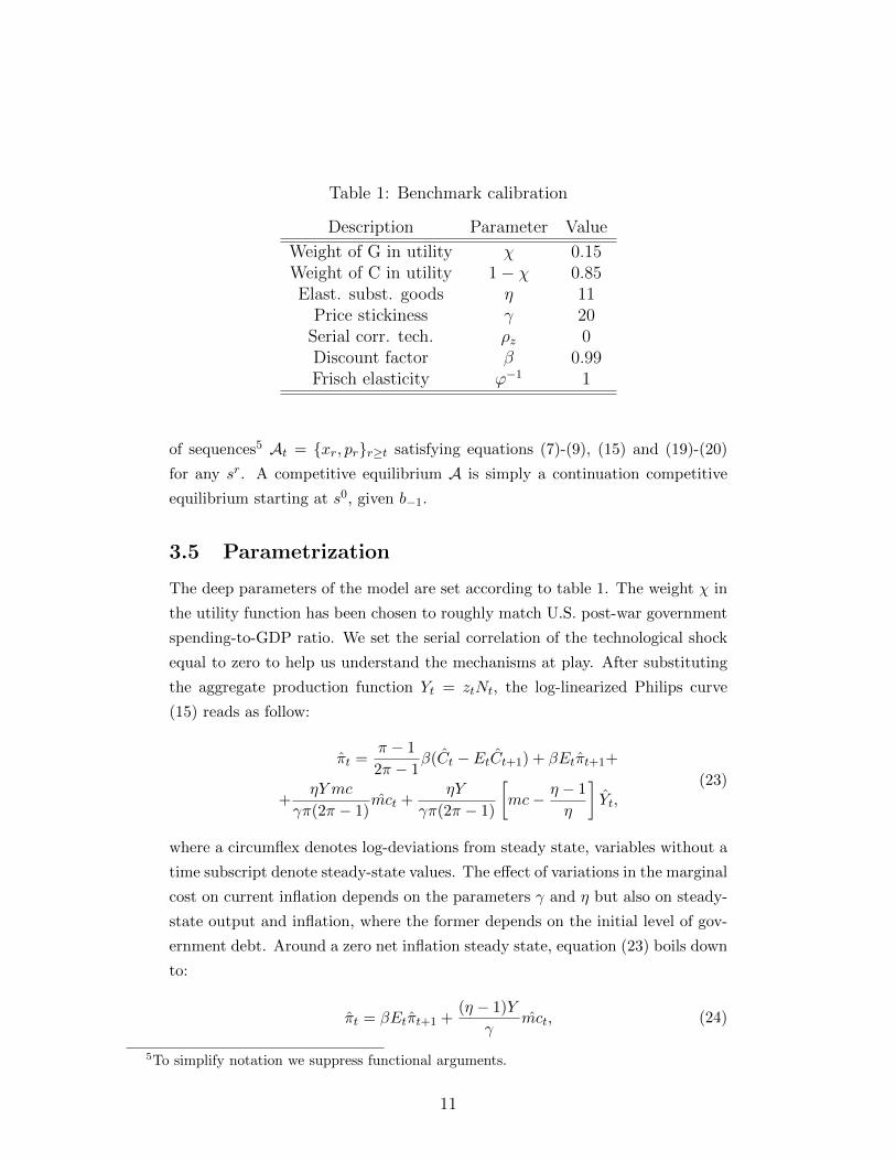
Table 1: Benchmark calibration

Description Parameter Value

Weight of G in utility χ 0.15Weight of C in utility 1− χ 0.85Elast. subst. goods η 11

Price stickiness γ 20Serial corr. tech. ρz 0Discount factor β 0.99Frisch elasticity ϕ−1 1

of sequences5 At = {xr, pr}r≥t satisfying equations (7)-(9), (15) and (19)-(20)

for any sr. A competitive equilibrium A is simply a continuation competitive

equilibrium starting at s0, given b−1.

3.5 Parametrization

The deep parameters of the model are set according to table 1. The weight χ in

the utility function has been chosen to roughly match U.S. post-war government

spending-to-GDP ratio. We set the serial correlation of the technological shock

equal to zero to help us understand the mechanisms at play. After substituting

the aggregate production function Yt = ztNt, the log-linearized Philips curve

(15) reads as follow:

πt =π − 1

2π − 1β(Ct − EtCt+1) + βEtπt+1+

+ηY mc

γπ(2π − 1)mct +

ηY

γπ(2π − 1)

[mc− η − 1

η

]Yt,

(23)

where a circumflex denotes log-deviations from steady state, variables without a

time subscript denote steady-state values. The effect of variations in the marginal

cost on current inflation depends on the parameters γ and η but also on steady-

state output and inflation, where the former depends on the initial level of gov-

ernment debt. Around a zero net inflation steady state, equation (23) boils down

to:

πt = βEtπt+1 +(η − 1)Y

γmct, (24)

5To simplify notation we suppress functional arguments.

11

taking the same form as in the Calvo model. Hence, we can establish a mapping

between our parametrization and average price duration. We set parameter γ

equal to 20 for our benchmark calibration, which implies a price duration of

roughly two quarters.

4 Pareto efficiency and policy coordination

We take as benchmarks Pareto efficiency and the case of perfect coordination,

where a single authority chooses monetary and fiscal policy instruments under

commitment. We refer to these benchmarks in section 6 to discuss the effects

of fiscal discretion under a variety of monetary regimes. The Pareto-efficient

allocation solves the problem of maximizing utility (1) subject to equations (2),

(10), (16), (21) and the resource constraint Yt(j) = Ct(j) + Gt(j) for any j. It

can be showed that Pareto efficiency requires Ct(j) = Ct, Yt(j) = Yt, Gt(j) = Gt

and Nt(j) = Nt. Moreover, the marginal rate of substitution between leisure and

private consumption and between leisure and public consumption must be equal

to the corresponding marginal rate of transformation. This implies

zt = Nϕt

Ct1− χ

= Nϕt

Gtχ. (25)

The optimality conditions yield the efficient allocation

N t = 1; Y t = zt; Ct = (1− χ)zt; Gt = χzt. (26)

Under Pareto efficiency hours worked are constant, while consumption, govern-

ment expenditure and output move proportionally to productivity. At the non-

stochastic steady state, where zt = 1 for all t, hours worked and output are

equal to 1, while private and public consumption are equal to 0.75 and 0.15,

respectively.

For the case of policy coordination, we follow the classic Ramsey (1927) ap-

proach and we define the optimal policy as a state-contingent plan. We refer

to this case as Full Ramsey (FR). We define an FR equilibrium as a compet-

itive equilibrium A0 that maximizes U0, given the initial condition b−1. The

lagrangian and the first-order conditions associated to the FR problem are re-

ported in appendix A.

Our benchmark economy features two distortions: a) imperfect competition

in the goods market; b) price-adjustment costs. After setting zt = 1 for all t,

12

we analyze the non-stochastic steady state of the Ramsey equilibrium and we

consider three steady-state levels of government debt.6 The first steady state

is the efficient equilibrium of our model. This is the allocation where a labor

subsidy completely eliminates the monopolistic distortion stemming from imper-

fect competition in the goods market. Since lump-sum taxes do not exist in our

model, the labor subsidy as well as the provision of the public good must be

financed with interest receipts on government assets. This implies that, at the

efficient steady state,

beff =1/η − χ1− β

, τ eff = − 1

η − 1.

The lagrangian multipliers on the government budget constraint λs, on the Euler

equation λb, and on the Phillips curve λp are equal to zero at the efficient steady

state. The values of the macroeconomic variables of interest are reported in

the third column of table 2. In words, public assets must be 24 times GDP for

the interest income to be sufficiently high to finance subsidies and government

spending. Since public assets are private liabilities in our model, the assumption

of commitment to repay on the side of private agents may appear unrealistic with

such high level of indebtedness. But we consider the efficient steady state as a

theoretical benchmark and maintain the assumption that all debts are repaid –

private or public. The second steady state features a positive level of government

debt that, without loss of generality, we set equal to GDP. In the third steady

state the government is a creditor and public assets are equal to GDP. These

two steady states are summarized in the fourth and fifth column of table 2. In

the economy with positive public debt the tax rate is 17.35% at the steady state.

The economy with public credit (negative public debt) has a steady-state tax

rate of 15.18%, which implies higher hours and output, relative to the economy

with positive public debt. However, in both cases hours worked, consumption

and output are well below their efficient levels. Even under perfect coordination

of monetary and fiscal policy, the economy fluctuates around a distorted steady

state, unless the government accumulates a large stock of public assets that may

be regarded as implausibly high.

In section 6, we inspect the dynamics of macroeconomic variables conditional

on technological shocks at the FR equilibrium and we compare it with dynamics

6More precisely, we choose the steady-state level of debt knowing that there exists an initial con-dition b−1 that supports it. We abstract from the transition from such initial condition to the chosensteady state.

13

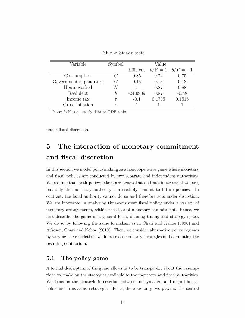
Table 2: Steady state

Variable Symbol ValueEfficient b/Y = 1 b/Y = −1

Consumption C 0.85 0.74 0.75Government expenditure G 0.15 0.13 0.13

Hours worked N 1 0.87 0.88Real debt b -24.0909 0.87 -0.88

Income tax τ -0.1 0.1735 0.1518Gross inflation π 1 1 1

Note: b/Y is quarterly debt-to-GDP ratio

under fiscal discretion.

5 The interaction of monetary commitment

and fiscal discretion

In this section we model policymaking as a noncooperative game where monetary

and fiscal policies are conducted by two separate and independent authorities.

We assume that both policymakers are benevolent and maximize social welfare,

but only the monetary authority can credibly commit to future policies. In

contrast, the fiscal authority cannot do so and therefore acts under discretion.

We are interested in analyzing time-consistent fiscal policy under a variety of

monetary arrangements, within the class of monetary commitment. Hence, we

first describe the game in a general form, defining timing and strategy space.

We do so by following the same formalism as in Chari and Kehoe (1990) and

Atkeson, Chari and Kehoe (2010). Then, we consider alternative policy regimes

by varying the restrictions we impose on monetary strategies and computing the

resulting equilibrium.

5.1 The policy game

A formal description of the game allows us to be transparent about the assump-

tions we make on the strategies available to the monetary and fiscal authorities.

We focus on the strategic interaction between policymakers and regard house-

holds and firms as non-strategic. Hence, there are only two players: the central

14

bank and the fiscal authority.

Timing – The events of the game unfold according to the following timeline. In

period t = 0, at a stage that one may consider as constitutional, the central bank

commits once and for all to a rule, say σm. Then, in every period t ≥ 0, a) shocks

occur and they are perfectly observed by all agents and authorities; b) the fiscal

authority chooses its fiscal tools; c) the monetary authority implements the plan

it committed to at the constitutional stage and economic variables realize. Vector

qt ≡ (zt, Gt, τt, it, xt) represents chronologically the events that occur in each

period. Accordingly, the history of the game can be defined as ht ≡ (qt, ht−1)

for t > 0 and h0 ≡ (q0, b−1) for t = 0. Our timing assumption implies that

the central bank leads both the fiscal policymaker and private agents, since it

chooses its policy at the constitutional stage. The fiscal policymaker only leads

private agents within each period. However, as it will become evident below, it

is convenient to think of the fiscal policymaker as a sequence of authorities with

identical preferences, each one leading her future selves.7

Histories, strategies and competitive equilibrium – The fiscal authority faces histo-

ries ht,f ≡ (ht−1, zt), i.e. it chooses government spending and taxes after observ-

ing ht−1 and the shock, so that its strategy is σf = {Gt(ht,f ), τt(ht,f )}t≥0. Sim-

ilarly, the monetary authority faces history ht,m ≡ (ht−1, zt, Gt, τt) and chooses

its instrument according to strategy σm = {it(ht,m)}t≥0. For any strategy, it is

convenient to define its continuation from a given history. For instance, consider

fiscal strategy σf . We denote its continuation as σtf = {Gr(hr,f ), τr(hr,f )}r≥t.Starting from any history ht−1, and given a sequence of exogenous events from

period t onward, fiscal and monetary strategies generate policies denoted by

{pr}r≥t, as in in section 3.4. Given policies, private agents face information

ht,x ≡ (ht−1, zt, Gt, τt, it) and take decisions according to σx = {xr}r≥t, where

xr are the decision rules defined in section 3.4. Hence, once monetary and fiscal

policy strategies are set, they generate a continuation competitive equilibrium

At = {xr, pr}r≥t from any history ht−1.

Strategy restrictions – We restrict to fiscal Markov strategies where fiscal in-

struments only respond to the inherited level of debt, bt−1, and the history of

7If one restricts to the case of monetary commitment, inverting the order of moves within eachperiod would not change our results. In fact, the central bank could still condition the nominal interestrate on the history of fiscal instruments.

15

exogenous events, st:8

Gt = Gt(st, bt−1); τt = τt(s

t, bt−1). (27)

We consider monetary strategies of the following form:

it(st, b−1, τt, Gt

)= (1 + iTt

(st, b−1

))

[πt

πTt (st, b−1, τt, Gt)

]φπ− 1. (28)

iTt and πTt denote the central bank’s targets for the nominal interest rate and in-

flation, respectively.9 The targets and the elasticity of the interest-rate response

to inflation φπ are predetermined at the constitutional stage; φπ is a constant

and we restrict it to guarantee that the system of equations (7)-(9), (15), (19)-

(20) and (27)-(28) has a locally unique solution. In particular, we assume that

φπ > 1/β so that the Taylor principle holds. We regard φπ as an institutional

parameter and we take it as given, the same way we assume that institutions

are designed to enforce monetary commitment. Section 7 discusses the optimal

choice of φπ from the welfare perspective. This particular class of monetary

strategies is appealing for various reasons. First, any competitive equilibrium

can be implemented by choosing σf and σm within the class defined by (27) and

(28). For example, consider a competitive equilibrium A and its continuations

At. Take (it, πt) ∈ A,(Gt, τt

)∈ At and specify monetary and fiscal strategies

as follows: Gt = Gt, τt = τt, iTt = it and πTt = πt. Then, A is the locally

unique solution to equations (7)-(9), (15), (19)-(20) and (27)-(28).10 In other

words, for any competitive equilibrium we can find a pair of rules, (27) and (28),

that can support it: our assumption on strategies is not particularly restrictive

and simplifies the solution of the game. Second, the monetary rule is flexible

enough to accommodate all the monetary policy regimes that we describe in the

following sections. Specifically, we consider the case of open-loop strategies in

section 5.2, where monetary policy does not respond to the actions of the fiscal

authority. We then consider the case of closed-loop strategies in sections 5.3 and

5.4, where the central bank conditions the interest rate to fiscal policy. In partic-

8When modeling discretion, it is standard to assume that the policy authority does not respondto past policies in order to exclude a multiplicity of reputational equilibria. Chari and Kehoe (1990),King, Lu and Pasten (2008) and Lu (2013) discuss the cases of trigger strategies and reputationmechanisms. We follow the literature and require differentiability of the fiscal strategies as in Klein,Krusell and Rios-Rull (2008), Debortoli and Nunes (2012) and Ellison and Rankin (2007).

9We omit functional arguments unless they are required to avoid ambiguities.10The proof is reported in appendix B.4.

16

ular, the central bank threatens to vary the nominal interest rate if fiscal policy

compromises the achievement of the inflation target, i.e. πt 6= πTt . In accordance

with the mandate of most inflation-targeting central banks, we assume that the

interest-rate rule does not directly target fiscal variables.

Markov-perfect fiscal policy – We always maintain the assumption that fiscal

decisions are Markov-perfect. Intuitively, the current fiscal authority chooses its

instruments Gt and τt taking into account that future fiscal policies will also be

chosen optimally. Formally, a fiscal strategy σ∗f is Markov-perfect if it maximizes

Ut for any ht,f and for any monetary strategy σm, given continuation σ∗,t+1f . We

adopt a primal approach and solve for the policy problem by deciding on both

policy variables and private decisions, subject to the constraint that they must

be a continuation competitive equilibrium. Hence, we look for a competitive

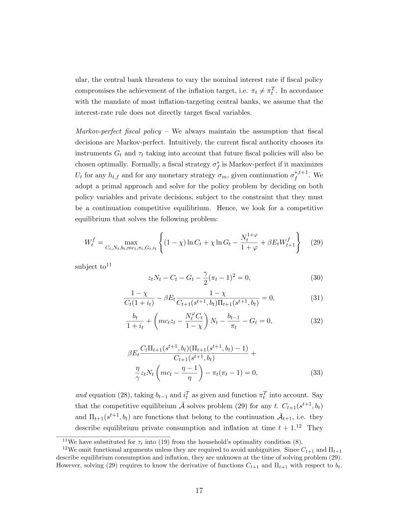
equilibrium that solves the following problem:

W ft = max

Ct,Nt,bt,mct,πt,Gt,it

{(1− χ) lnCt + χ lnGt −

N1+ϕt

1 + ϕ+ βEtW

ft+1

}(29)

subject to11

ztNt − Ct −Gt −γ

2(πt − 1)2 = 0, (30)

1− χCt(1 + it)

− βEt1− χ

Ct+1(st+1, bt)Πt+1(st+1, bt)= 0, (31)

bt1 + it

+

(mctzt −

Nϕt Ct

1− χ

)Nt −

bt−1

πt−Gt = 0, (32)

βEtCtΠt+1(st+1, bt)(Πt+1(st+1, bt)− 1)

Ct+1(st+1, bt)+

η

γztNt

(mct −

η − 1

η

)− πt(πt − 1) = 0, (33)

and equation (28), taking bt−1 and iTt as given and function πTt into account. Say

that the competitive equilibrium A solves problem (29) for any t. Ct+1(st+1, bt)

and Πt+1(st+1, bt) are functions that belong to the continuation At+1, i.e. they

describe equilibrium private consumption and inflation at time t + 1.12 They

11We have substituted for τt into (19) from the household’s optimality condition (8).12We omit functional arguments unless they are required to avoid ambiguities. Since Ct+1 and Πt+1

describe equilibrium consumption and inflation, they are unknown at the time of solving problem (29).However, solving (29) requires to know the derivative of functions Ct+1 and Πt+1 with respect to bt.

17

are taken as given by the fiscal authority because it cannot commit to future

outcomes. However, the current level of debt, bt, affects future inflation and con-

sumption, which in turn enter the fiscal decision problem via equations (31) and

(33). We assume that the fiscal policymaker internalizes this effect to guarantee

Markov-perfection. Rules Gt(st, bt−1) and τt(s

t, bt−1) are an equilibrium fiscal

strategy if they belong to continuations At for any t.

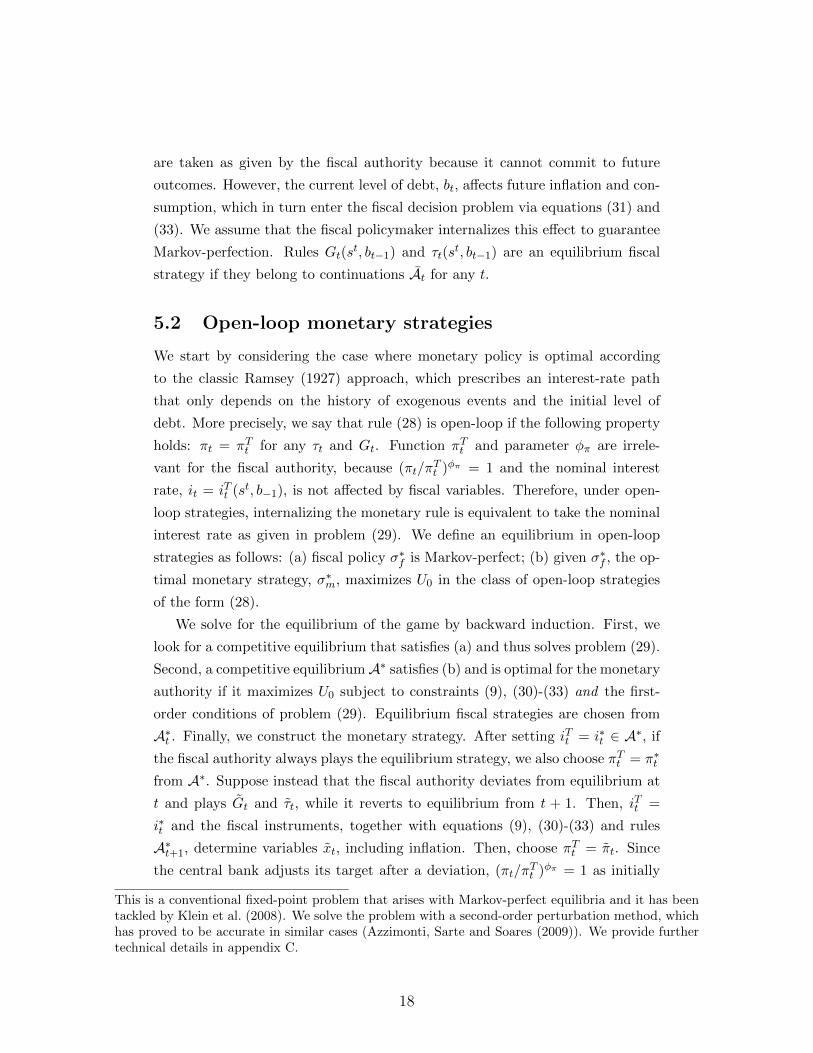
5.2 Open-loop monetary strategies

We start by considering the case where monetary policy is optimal according

to the classic Ramsey (1927) approach, which prescribes an interest-rate path

that only depends on the history of exogenous events and the initial level of

debt. More precisely, we say that rule (28) is open-loop if the following property

holds: πt = πTt for any τt and Gt. Function πTt and parameter φπ are irrele-

vant for the fiscal authority, because (πt/πTt )φπ = 1 and the nominal interest

rate, it = iTt (st, b−1), is not affected by fiscal variables. Therefore, under open-

loop strategies, internalizing the monetary rule is equivalent to take the nominal

interest rate as given in problem (29). We define an equilibrium in open-loop

strategies as follows: (a) fiscal policy σ∗f is Markov-perfect; (b) given σ∗f , the op-

timal monetary strategy, σ∗m, maximizes U0 in the class of open-loop strategies

of the form (28).

We solve for the equilibrium of the game by backward induction. First, we

look for a competitive equilibrium that satisfies (a) and thus solves problem (29).

Second, a competitive equilibriumA∗ satisfies (b) and is optimal for the monetary

authority if it maximizes U0 subject to constraints (9), (30)-(33) and the first-

order conditions of problem (29). Equilibrium fiscal strategies are chosen from

A∗t . Finally, we construct the monetary strategy. After setting iTt = i∗t ∈ A∗, if

the fiscal authority always plays the equilibrium strategy, we also choose πTt = π∗t

from A∗. Suppose instead that the fiscal authority deviates from equilibrium at

t and plays Gt and τt, while it reverts to equilibrium from t + 1. Then, iTt =

i∗t and the fiscal instruments, together with equations (9), (30)-(33) and rules

A∗t+1, determine variables xt, including inflation. Then, choose πTt = πt. Since

the central bank adjusts its target after a deviation, (πt/πTt )φπ = 1 as initially

This is a conventional fixed-point problem that arises with Markov-perfect equilibria and it has beentackled by Klein et al. (2008). We solve the problem with a second-order perturbation method, whichhas proved to be accurate in similar cases (Azzimonti, Sarte and Soares (2009)). We provide furthertechnical details in appendix C.

18

assumed, irrespective of whether fiscal policy deviates from equilibrium or not.

Notice that even if the monetary instrument does not respond to fiscal policy, the

central bank fully internalizes fiscal behavior: the optimality conditions of the

fiscal policy problem (29) are taken into account in the monetary policy problem.

In words, realized interest rate and inflation coincide with their corresponding

targets, which fully describe the Ramsey optimal monetary policy under fiscal

discretion. Should fiscal policy threaten the achievement of the inflation target,

an event that is never observed at equilibrium, the central bank sticks to the

announced interest rate but it compromises on its inflation target: the central

bank stands ready to accommodate fiscal ‘misbehavior’. The formal problem is

presented in appendix B.1.

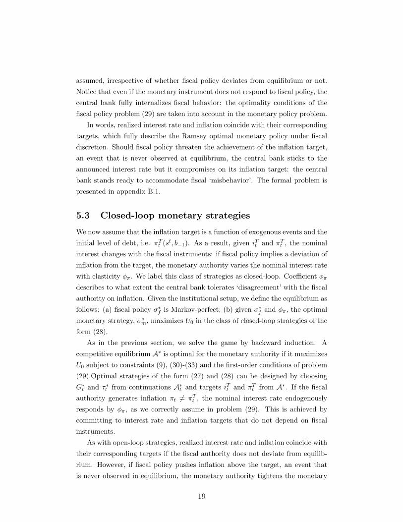
5.3 Closed-loop monetary strategies

We now assume that the inflation target is a function of exogenous events and the

initial level of debt, i.e. πTt (st, b−1). As a result, given iTt and πTt , the nominal

interest changes with the fiscal instruments: if fiscal policy implies a deviation of

inflation from the target, the monetary authority varies the nominal interest rate

with elasticity φπ. We label this class of strategies as closed-loop. Coefficient φπ

describes to what extent the central bank tolerates ‘disagreement’ with the fiscal

authority on inflation. Given the institutional setup, we define the equilibrium as

follows: (a) fiscal policy σ∗f is Markov-perfect; (b) given σ∗f and φπ, the optimal

monetary strategy, σ∗m, maximizes U0 in the class of closed-loop strategies of the

form (28).

As in the previous section, we solve the game by backward induction. A

competitive equilibrium A∗ is optimal for the monetary authority if it maximizes

U0 subject to constraints (9), (30)-(33) and the first-order conditions of problem

(29).Optimal strategies of the form (27) and (28) can be designed by choosing

G∗t and τ∗t from continuations A∗t and targets iTt and πTt from A∗. If the fiscal

authority generates inflation πt 6= πTt , the nominal interest rate endogenously

responds by φπ, as we correctly assume in problem (29). This is achieved by

committing to interest rate and inflation targets that do not depend on fiscal

instruments.

As with open-loop strategies, realized interest rate and inflation coincide with

their corresponding targets if the fiscal authority does not deviate from equilib-

rium. However, if fiscal policy pushes inflation above the target, an event that

is never observed in equilibrium, the monetary authority tightens the monetary

19

policy stance. This off-equilibrium response affects the behavior of the fiscal

authority, as we illustrate below by comparing open- and closed-loop strategies.

The formal problem is presented in appendix B.2.

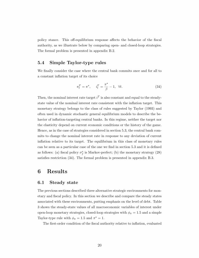
5.4 Simple Taylor-type rules

We finally consider the case where the central bank commits once and for all to

a constant inflation target of its choice

πTt = π∗, iTt =π∗

β− 1, ∀t. (34)

Then, the nominal interest rate target iT is also constant and equal to the steady-

state value of the nominal interest rate consistent with the inflation target. This

monetary strategy belongs to the class of rules suggested by Taylor (1993) and

often used in dynamic stochastic general equilibrium models to describe the be-

havior of inflation-targeting central banks. In this regime, neither the target nor

the elasticity depend on current economic conditions or the history of the game.

Hence, as in the case of strategies considered in section 5.3, the central bank com-

mits to change the nominal interest rate in response to any deviation of current

inflation relative to its target. The equilibrium in this class of monetary rules

can be seen as a particular case of the one we find in section 5.3 and it is defined

as follows: (a) fiscal policy σ∗f is Markov-perfect; (b) the monetary strategy (28)

satisfies restriction (34). The formal problem is presented in appendix B.3.

6 Results

6.1 Steady state

The previous sections described three alternative strategic environments for mon-

etary and fiscal policy. In this section we describe and compare the steady states

associated with these environments, putting emphasis on the level of debt. Table

3 shows the steady-state values of all macroeconomic variables of interest under

open-loop monetary strategies, closed-loop strategies with φπ = 1.5 and a simple

Taylor-type rule with φπ = 1.5 and π∗ = 1.

The first-order condition of the fiscal authority relative to inflation, evaluated

20

at the steady state, implies

−λsb

π2(βφπ − 1)− λfγ(π − 1)− λp(2π − 1)− βφπ

λb

Cπ2= 0, (35)

where λs ≥ 0 is the lagrangian multiplier for the government budget constraint,

λf ≥ 0 for the resource constraint, λp ≤ 0 for the Phillips curve and λb for

the Euler equation.13 The first term captures the effect of inflation on public

accounts. An increase in current inflation reduces debt repayment but raises the

nominal interest rate with elasticity φπ. If φπ > 1/β and the real interest rate

also increases, inflation leads to a loss in real terms and the government has an

incentive to generate deflation if it is a debtor. If instead the central bank does

not respond to the actions of fiscal policy, the impact of inflation on the real cost

of debt is only given by λsb/π2: positive debt gives the incentive to generate

inflation, negative debt to reduce it. The second term is the resource cost, which

disappears if net inflation is zero or if prices are fully flexible (γ = 0). The third

term captures the benefits from reduced price markups. With sticky prices an

increase in trend inflation reduces the average markup and raises output, which

is sub-optimally low due to monopolistic competition. The last term is the effect

on consumption smoothing. Higher inflation leads to lower government bond

prices. Households are thus willing to defer consumption and ceteris paribus

public debt tends to increase. This effect raises or reduces welfare, depending on

how debt accumulation affects the inflation-output tradeoff. From the first-order

condition relative to debt

λb

Cπ2= −λp

∂Π∂btC(2π − 1)− ∂C

∂btπ(π − 1)

∂Π∂btC + ∂C

∂btπ

. (36)

Under our calibration, the denominator on the right-hand side of (36) is posi-

tive under all monetary policy regimes. If the numerator is also positive, debt

accumulation increases the forward-looking component of the Phillips curve and

worsens the inflation-output tradeoff. As we discuss below, the monetary regime

determines whether debt accumulation improves or worsens the inflation-output

tradeoff and thus the sign of λb/Cπ2.

13We substitute the lagrangian multipliers for the monetary rule, λi, by using the first-order con-dition relative to the nominal interest rate. Even if we require φπ > 1/β across all monetary policyregimes, equation (35) nests the case of open-loop monetary strategies for φπ = 0. Under open-loopstrategies, the central bank always adjusts its inflation target in such a way that the nominal interestrate does not respond to the actions of the fiscal authority. Hence, it is as if φπ was zero in (35).

21

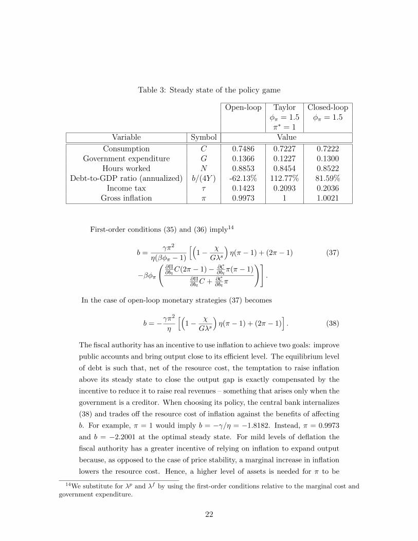
Table 3: Steady state of the policy game

Open-loop Taylor Closed-loopφπ = 1.5 φπ = 1.5π∗ = 1

Variable Symbol Value

Consumption C 0.7486 0.7227 0.7222Government expenditure G 0.1366 0.1227 0.1300

Hours worked N 0.8853 0.8454 0.8522Debt-to-GDP ratio (annualized) b/(4Y ) -62.13% 112.77% 81.59%

Income tax τ 0.1423 0.2093 0.2036Gross inflation π 0.9973 1 1.0021

First-order conditions (35) and (36) imply14

b =γπ2

η(βφπ − 1)

[(1− χ

Gλs

)η(π − 1) + (2π − 1) (37)

−βφπ

(∂Π∂btC(2π − 1)− ∂C

∂btπ(π − 1)

∂Π∂btC + ∂C

∂btπ

)].

In the case of open-loop monetary strategies (37) becomes

b = −γπ2

η

[(1− χ

Gλs

)η(π − 1) + (2π − 1)

]. (38)

The fiscal authority has an incentive to use inflation to achieve two goals: improve

public accounts and bring output close to its efficient level. The equilibrium level

of debt is such that, net of the resource cost, the temptation to raise inflation

above its steady state to close the output gap is exactly compensated by the

incentive to reduce it to raise real revenues – something that arises only when the

government is a creditor. When choosing its policy, the central bank internalizes

(38) and trades off the resource cost of inflation against the benefits of affecting

b. For example, π = 1 would imply b = −γ/η = −1.8182. Instead, π = 0.9973

and b = −2.2001 at the optimal steady state. For mild levels of deflation the

fiscal authority has a greater incentive of relying on inflation to expand output

because, as opposed to the case of price stability, a marginal increase in inflation

lowers the resource cost. Hence, a higher level of assets is needed for π to be

14We substitute for λp and λf by using the first-order conditions relative to the marginal cost andgovernment expenditure.

22

a steady state. The central bank thus accepts some deflation to increase public

assets, reduce taxes and improve welfare. When prices are flexible or the output

gap is zero (η →∞), the optimal level of debt is zero, as highlighted by Debortoli

and Nunes (2012).

In the case of a simple Taylor-type rule with π∗ = π = 1, (37) simplifies to

b =γ

η(βφπ − 1)

(1− βφπ

∂Π∂btC

∂Π∂btC + ∂C

∂bt

). (39)

Differently from the case of open-loop strategies, the real interest rate rises if

inflation deviates from its target π∗. The central bank’s response generates two

counteracting effects. On the one hand, it makes inflationary policies costly by

reducing the government’s real revenues. Such cost increases in φπ and b as high-

lighted in (35). On the other hand, the deterioration in public accounts triggers

debt accumulation, which in turn encourages the future fiscal authority to re-

duce inflation. Hence, expected inflation falls and the inflation-output tradeoff

improves. This effect is captured by the term ∂Π/∂bt, which is indeed nega-

tive for our calibration. In this respect, a larger φπ makes inflationary policies

less costly. At the optimal steady state, debt is such that the gain of inflating

to close the output gap is exactly compensated by the gain of reducing debt

servicing costs – something that arises only when the government is a debtor.

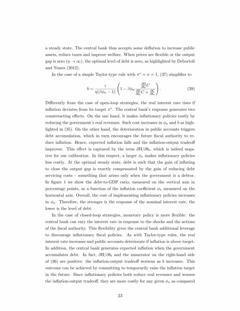
In figure 1 we show the debt-to-GDP ratio, measured on the vertical axis in

percentage points, as a function of the inflation coefficient φπ measured on the

horizontal axis. Overall, the cost of implementing inflationary policies increases

in φπ. Therefore, the stronger is the response of the nominal interest rate, the

lower is the level of debt.

In the case of closed-loop strategies, monetary policy is more flexible: the

central bank can vary the interest rate in response to the shocks and the actions

of the fiscal authority. This flexibility gives the central bank additional leverage

to discourage inflationary fiscal policies. As with Taylor-type rules, the real

interest rate increases and public accounts deteriorate if inflation is above target.

In addition, the central bank generates expected inflation when the government

accumulates debt. In fact, ∂Π/∂bt and the numerator on the right-hand side

of (36) are positive: the inflation-output tradeoff worsens as b increases. This

outcome can be achieved by committing to temporarily raise the inflation target

in the future. Since inflationary policies both reduce real revenues and worsen

the inflation-output tradeoff, they are more costly for any given φπ as compared

23

0.0

0.2

0.4

0.6

0.8

1.0

1.2

1.5 1.75 2 2.25 2.5 2.75 3 3.25 3.5

b/(

4 Y

)

φπ

Taylor closed-loop

Figure 1: Debt-to-GDP (annualized) ratio as function of φπ

to Taylor-type rules. Therefore, debt is lower as showed in figure 1. Finally, the

central bank deviates from price stability. For example, table 3 shows that for

φπ = 1.5 a mildly positive inflation rate is optimal. This is because it makes the

fiscal authority less willing to rely on inflation and a lower level of debt is needed

to discipline discretionary fiscal behavior. We find however that irrespective of

φπ the inflation rate is small and we conclude that price stability is roughly

optimal.

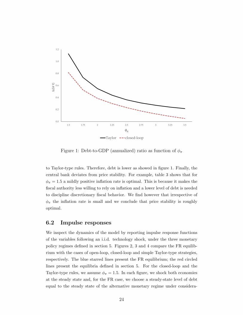
6.2 Impulse responses

We inspect the dynamics of the model by reporting impulse response functions

of the variables following an i.i.d. technology shock, under the three monetary

policy regimes defined in section 5. Figures 2, 3 and 4 compare the FR equilib-

rium with the cases of open-loop, closed-loop and simple Taylor-type strategies,

respectively. The blue starred lines present the FR equilibrium; the red circled

lines present the equilibria defined in section 5. For the closed-loop and the

Taylor-type rules, we assume φπ = 1.5. In each figure, we shock both economies

at the steady state and, for the FR case, we choose a steady-state level of debt

equal to the steady state of the alternative monetary regime under considera-

24

tion.15 We fix the size of the shock to the typical standard deviation considered

in the business cycle literature, 0.0071. Then we normalize consumption, gov-

ernment expenditure, hours worked and output with respect to the shock and

we report them in percentage deviations from the steady state. Hence, a one-

percent increase in a given variable means that the variable increases as much as

productivity. Inflation and the nominal interest rate are not normalized. They

are rather expressed in deviation from the steady state and in percentage points,

so that they can be read as rates. Finally, tax rates and real debt are not normal-

ized either and they are reported in percentage deviations from their steady-state

values. We limit our attention to the case where γ = 20 and price adjustments

are costly.16

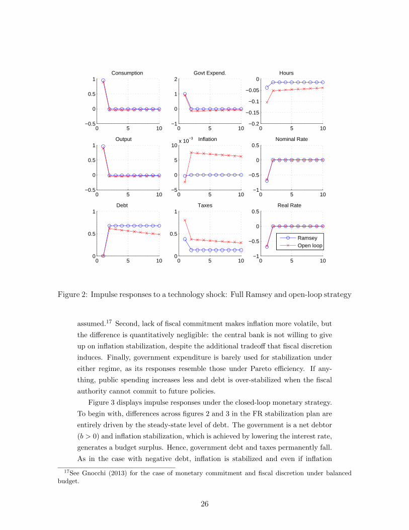
Figure 2 evaluates the open-loop monetary strategy against the FR model.

In the latter regime inflation is stabilized, since changing prices is costly. The

real interest rate falls, which leads to lower revenues because the government is

a net creditor (b < 0). Labor income taxes remain fairly stable so that hours

worked are stabilized; the nominal interest rate is reduced so as to raise private

consumption. Increased tax revenues due to higher wages finance an increase

in public spending. The response of output and consumption, both private and

public, well approximate Pareto-efficiency. Inflation stabilization has two conse-

quences. First, since the government is a creditor, it generates a budget deficit in

the short run. Second, it induces a unit root in public debt that turns short-run

budget imbalances in long-run debt changes. By comparing the open-loop strat-

egy regime with the FR case, three facts stand out. Fiscal discretion worsens

the tradeoff between stabilizing inflation and real activity, as it becomes clear by

looking at the response of hours worked. Should the current fiscal authority limit

the tax rise, future governments would be endowed with a lower credit and they

would find it optimal to inflate, as we explain in the steady-state section. Since

expected inflation worsens the current inflation-output tradeoff, the government

decides to raise taxes so as to contain public deficits and future inflation. As

a result, hours worked fall. Such tradeoff is absent when balanced budget is

15In the FR case, for any chosen steady-state level of debt, there exists an initial condition b−1 thatsupports it. We do not analyze the transition from t = 0 to the steady state.

16The Ramsey problem with flexible prices has been analyzed by Lucas and Stokey (1983) andChari et al. (1991). If initial nominal public assets are negative, the optimal price level at time zero isinfinite so that the distorting labor income tax is reduced. If initial nominal public assets are positive,the optimal monetary policy at time zero is the one that implements the efficient allocation. We donot repeat this analysis here.

25

0 5 10−0.5

0

0.5

1Consumption

0 5 10−1

0

1

2Govt Expend.

0 5 10−0.2

−0.15

−0.1

−0.05

0Hours

0 5 10−0.5

0

0.5

1Output

0 5 10−5

0

5

10x 10

−3 Inflation

0 5 10−1

−0.5

0

0.5Nominal Rate

0 5 100

0.5

1Debt

0 5 100

0.5

1Taxes

0 5 10−1

−0.5

0

0.5Real Rate

RamseyOpen loop

Figure 2: Impulse responses to a technology shock: Full Ramsey and open-loop strategy

assumed.17 Second, lack of fiscal commitment makes inflation more volatile, but

the difference is quantitatively negligible: the central bank is not willing to give

up on inflation stabilization, despite the additional tradeoff that fiscal discretion

induces. Finally, government expenditure is barely used for stabilization under

either regime, as its responses resemble those under Pareto efficiency. If any-

thing, public spending increases less and debt is over-stabilized when the fiscal

authority cannot commit to future policies.

Figure 3 displays impulse responses under the closed-loop monetary strategy.

To begin with, differences across figures 2 and 3 in the FR stabilization plan are

entirely driven by the steady-state level of debt. The government is a net debtor

(b > 0) and inflation stabilization, which is achieved by lowering the interest rate,

generates a budget surplus. Hence, government debt and taxes permanently fall.

As in the case with negative debt, inflation is stabilized and even if inflation

17See Gnocchi (2013) for the case of monetary commitment and fiscal discretion under balancedbudget.

26

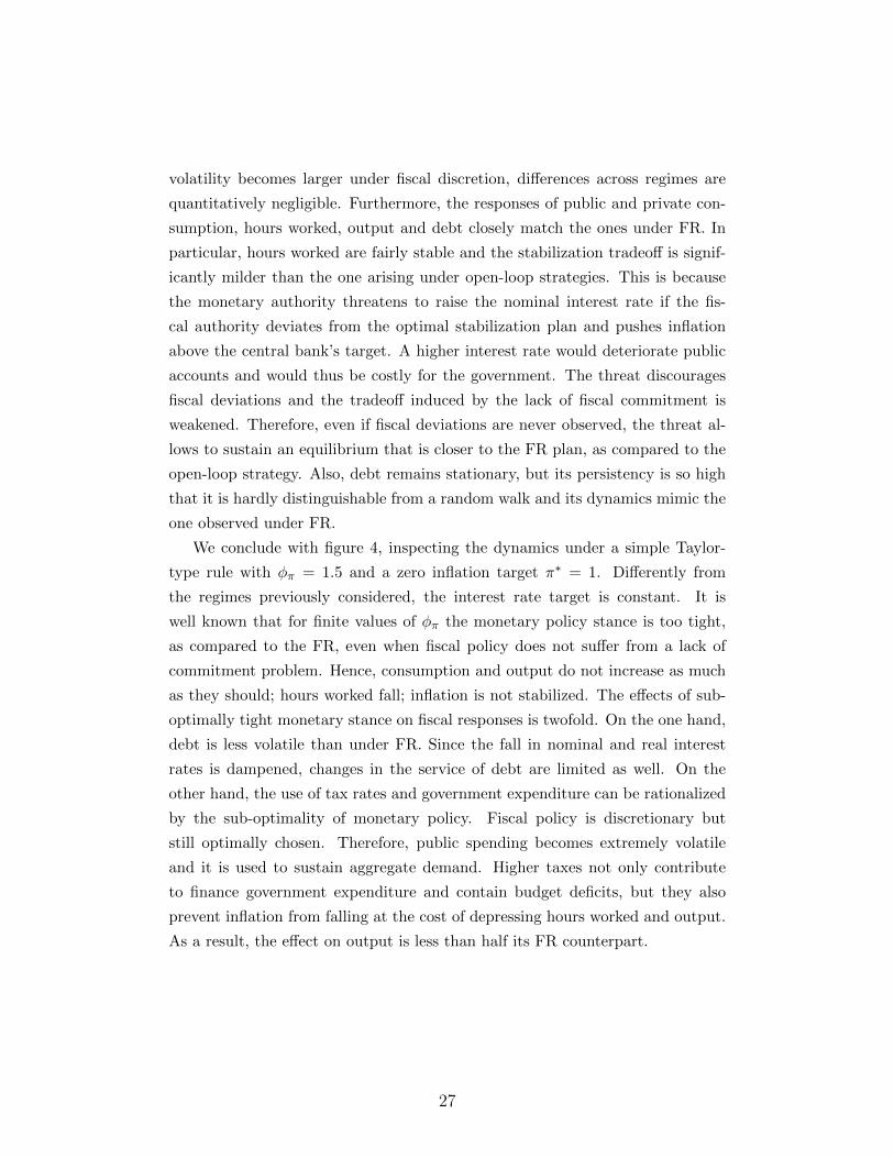
volatility becomes larger under fiscal discretion, differences across regimes are

quantitatively negligible. Furthermore, the responses of public and private con-

sumption, hours worked, output and debt closely match the ones under FR. In

particular, hours worked are fairly stable and the stabilization tradeoff is signif-

icantly milder than the one arising under open-loop strategies. This is because

the monetary authority threatens to raise the nominal interest rate if the fis-

cal authority deviates from the optimal stabilization plan and pushes inflation

above the central bank’s target. A higher interest rate would deteriorate public

accounts and would thus be costly for the government. The threat discourages

fiscal deviations and the tradeoff induced by the lack of fiscal commitment is

weakened. Therefore, even if fiscal deviations are never observed, the threat al-

lows to sustain an equilibrium that is closer to the FR plan, as compared to the

open-loop strategy. Also, debt remains stationary, but its persistency is so high

that it is hardly distinguishable from a random walk and its dynamics mimic the

one observed under FR.

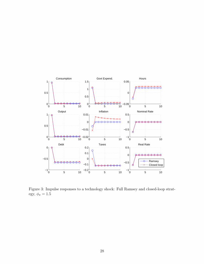
We conclude with figure 4, inspecting the dynamics under a simple Taylor-

type rule with φπ = 1.5 and a zero inflation target π∗ = 1. Differently from

the regimes previously considered, the interest rate target is constant. It is

well known that for finite values of φπ the monetary policy stance is too tight,

as compared to the FR, even when fiscal policy does not suffer from a lack of

commitment problem. Hence, consumption and output do not increase as much

as they should; hours worked fall; inflation is not stabilized. The effects of sub-

optimally tight monetary stance on fiscal responses is twofold. On the one hand,

debt is less volatile than under FR. Since the fall in nominal and real interest

rates is dampened, changes in the service of debt are limited as well. On the

other hand, the use of tax rates and government expenditure can be rationalized

by the sub-optimality of monetary policy. Fiscal policy is discretionary but

still optimally chosen. Therefore, public spending becomes extremely volatile

and it is used to sustain aggregate demand. Higher taxes not only contribute

to finance government expenditure and contain budget deficits, but they also

prevent inflation from falling at the cost of depressing hours worked and output.

As a result, the effect on output is less than half its FR counterpart.

27

0 5 100

0.5

1Consumption

0 5 100

0.5

1

1.5Govt Expend.

0 5 10−0.05

0

0.05Hours

0 5 100

0.5

1Output

0 5 10−0.02

−0.01

0

0.01Inflation

0 5 10−1

−0.5

0

0.5Nominal Rate

0 5 10−1

−0.5

0Debt

0 5 10−0.2

−0.1

0

0.1

0.2Taxes

0 5 10−1

−0.5

0

0.5Real Rate

RamseyClosed loop

Figure 3: Impulse responses to a technology shock: Full Ramsey and closed-loop strat-egy, φπ = 1.5

28

0 5 10−0.5

0

0.5

1Consumption

0 5 100

0.5

1

1.5

2Govt Expend.

0 5 10−1

−0.5

0

0.5Hours

0 5 100

0.5

1Output

0 5 10−0.1

−0.05

0

0.05

0.1Inflation

0 5 10−1

−0.5

0

0.5Nominal Rate

0 5 10−1

−0.5

0Debt

0 5 10−2

0

2

4Taxes

0 5 10−1

−0.5

0

0.5Real Rate

RamseyTaylor

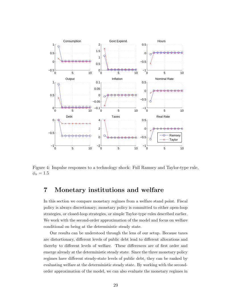
Figure 4: Impulse responses to a technology shock: Full Ramsey and Taylor-type rule,φπ = 1.5

7 Monetary institutions and welfare

In this section we compare monetary regimes from a welfare stand point. Fiscal

policy is always discretionary; monetary policy is committed to either open-loop

strategies, or closed-loop strategies, or simple Taylor-type rules described earlier.

We work with the second-order approximation of the model and focus on welfare

conditional on being at the deterministic steady state.

Our results can be understood through the lens of our setup. Because taxes

are distortionary, different levels of public debt lead to different allocations and

thereby to different levels of welfare. These differences are of first order and

emerge already at the deterministic steady state. Since the three monetary policy

regimes have different steady-state levels of public debt, they can be ranked by

evaluating welfare at the deterministic steady state. By working with the second-

order approximation of the model, we can also evaluate the monetary regimes in

29

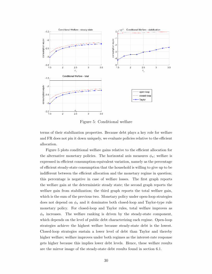
Figure 5: Conditional welfare

terms of their stabilization properties. Because debt plays a key role for welfare

and FR does not pin it down uniquely, we evaluate policies relative to the efficient

allocation.

Figure 5 plots conditional welfare gains relative to the efficient allocation for

the alternative monetary policies. The horizontal axis measures φπ; welfare is

expressed in efficient consumption-equivalent variation, namely as the percentage

of efficient steady-state consumption that the household is willing to give up to be

indifferent between the efficient allocation and the monetary regime in question;

this percentage is negative in case of welfare losses. The first graph reports

the welfare gain at the deterministic steady state; the second graph reports the

welfare gain from stabilization; the third graph reports the total welfare gain,

which is the sum of the previous two. Monetary policy under open-loop strategies

does not depend on φπ and it dominates both closed-loop and Taylor-type rule

monetary policy. For closed-loop and Taylor rules, total welfare improves as

φπ increases. The welfare ranking is driven by the steady-state component,

which depends on the level of public debt characterizing each regime. Open-loop

strategies achieve the highest welfare because steady-state debt is the lowest.

Closed-loop strategies sustain a lower level of debt than Taylor and thereby

higher welfare; welfare improves under both regimes as the interest-rate response

gets higher because this implies lower debt levels. Hence, these welfare results

are the mirror image of the steady-state debt results found in section 6.1.

30

Closed-loop strategies are characterized by the highest stabilization com-

ponent, even better than open-loop strategies. As emphasized in section 6.2,

closed-loop strategies sustain equilibrium responses to technology shocks that

are much closer to FR than open-loop strategies. This is because the govern-

ment is a debtor (b > 0) under closed-loop strategies and the monetary author-

ity’s threat to raise the nominal interest rate would deteriorate the government

budget, thereby discouraging fiscal deviations. Taylor ranks worst in terms of

stabilization because monetary policy is too tight and fiscal responses strongly

sub-optimal. We focus on technology shocks, but considering additional exoge-

nous shocks is unlikely to change the ranking in terms of welfare because the

stabilization component is small relative to the steady-state counterpart.

What do we learn for the design of monetary policy institutions? Two results

emerge from our analysis. First, and most important, monetary policy plays a

key role in the determination of public debt. Starting from the work of Sargent

and Wallace (1981), many contributions have studied how monetary policy af-

fects fiscal policy. Our new insight is that commitment to raising the real interest

rate in response to inflation leads to a unique and positive level of debt; a higher

interest-rate elasticity to inflation leads to lower debt and higher welfare. Sec-

ond, the simple interest-rate rule studied here approximates relatively well the

sophisticated closed-loop rule. Being able to change the state-contingent infla-

tion target and to commit to off-equilibrium responses helps in achieving better

stabilization and slightly lower public debt, but it is the interest-rate response

that pins down debt and welfare.

Optimal monetary policy in the sense of Ramsey is difficult to implement

in reality; for this reason central banks have been adopting simple interest-rate

rules, which can be easily communicated to and observed by agents. Our Taylor-

type rule belongs to this class of monetary policies and it features two parameters:

the elasticity to the interest rate φπ and the inflation target π∗. Keeping the

inflation target constant and equal to one, an increase in φπ raises welfare, as

shown in Figure 5; changing the elasticity from 1.5 to 3.5 delivers a welfare gain of

0.8 percentage point in consumption-equivalent terms. Changes in the inflation

target, however, also affect welfare. An increase in the inflation target is costly

due to price-adjustment costs, so that the incentive to raise inflation to close

the output gap is reduced. As a result, the steady-state level of debt is lower (in

absolute value) and welfare improves. Figure 6 plots the welfare gain of optimally

choosing the inflation target. Net inflation, annual and in percentage points, is

31

0

1

2

3

4

5

6

7

1.5 1.7 1.9 2.1 2.3 2.5 2.7 2.9 3.1 3.3 3.50.00

0.05

0.10

0.15

0.20

0.25

0.30

0.35

Welfare gain (2nd axis) Optimal inflation target

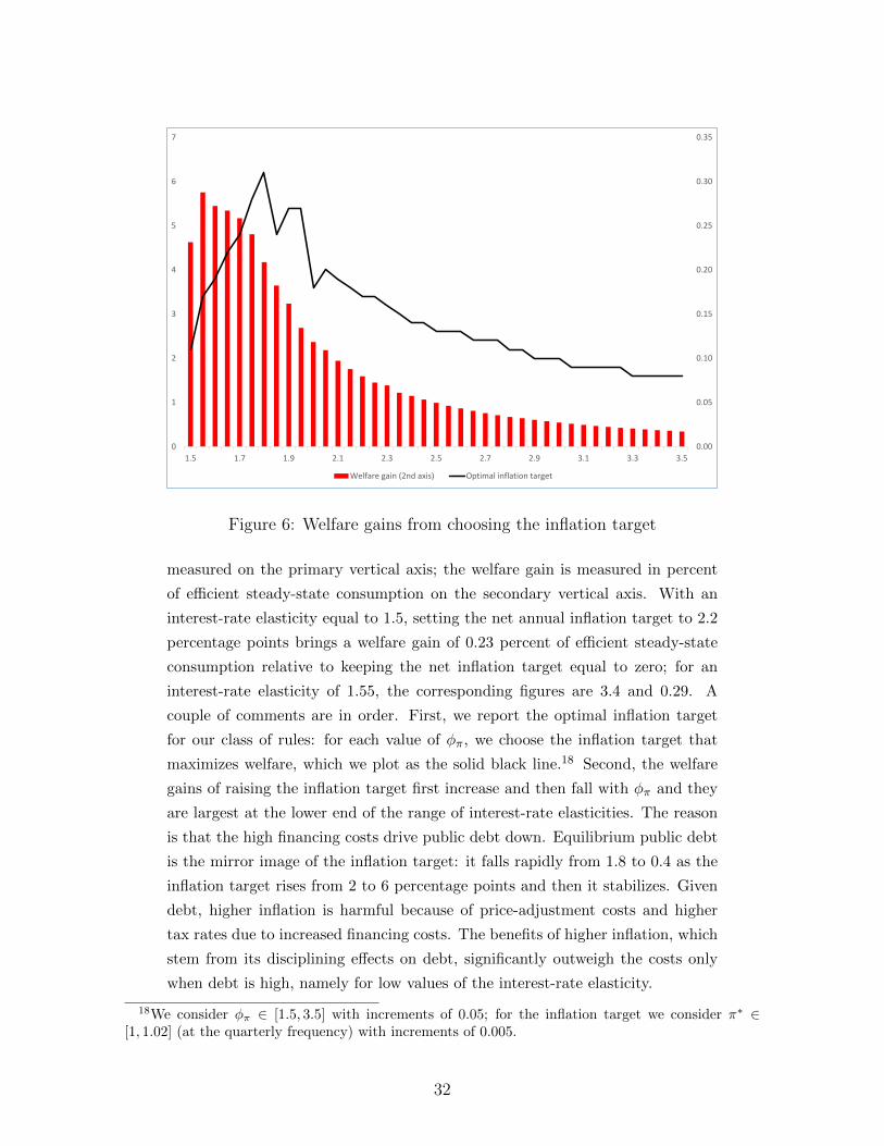
Figure 6: Welfare gains from choosing the inflation target

measured on the primary vertical axis; the welfare gain is measured in percent

of efficient steady-state consumption on the secondary vertical axis. With an

interest-rate elasticity equal to 1.5, setting the net annual inflation target to 2.2

percentage points brings a welfare gain of 0.23 percent of efficient steady-state

consumption relative to keeping the net inflation target equal to zero; for an

interest-rate elasticity of 1.55, the corresponding figures are 3.4 and 0.29. A

couple of comments are in order. First, we report the optimal inflation target

for our class of rules: for each value of φπ, we choose the inflation target that

maximizes welfare, which we plot as the solid black line.18 Second, the welfare

gains of raising the inflation target first increase and then fall with φπ and they

are largest at the lower end of the range of interest-rate elasticities. The reason

is that the high financing costs drive public debt down. Equilibrium public debt

is the mirror image of the inflation target: it falls rapidly from 1.8 to 0.4 as the

inflation target rises from 2 to 6 percentage points and then it stabilizes. Given

debt, higher inflation is harmful because of price-adjustment costs and higher

tax rates due to increased financing costs. The benefits of higher inflation, which

stem from its disciplining effects on debt, significantly outweigh the costs only

when debt is high, namely for low values of the interest-rate elasticity.

18We consider φπ ∈ [1.5, 3.5] with increments of 0.05; for the inflation target we consider π∗ ∈[1, 1.02] (at the quarterly frequency) with increments of 0.005.

32

8 Conclusions

The design of monetary and fiscal policy institutions emphasizes independence

in setting the policy instrument. Central banks are wary to comment on fiscal

policy; governments are supposed not to pressure monetary policy. In the EMU,

this independence is reinforced by the prohibition of monetary financing of bud-

gets, namely the explicit interdiction to the ECB to purchase government debt

on the primary market. On these grounds, the German Constitutional Court

questioned the consistency of ECB’s OMT announcement with the EU primary

law. These recent events illustrate the tension behind this division of powers.

Our analysis assumes independence. Nevertheless, we show that monetary

and fiscal policy inevitably interact in several dimensions via a) the strategic

setup; b) the ability to commit future actions and responses; c) the general

equilibrium effect on the economy. As a result of these interactions, monetary

commitment to an interest-rate response to deviation of inflation from its tar-

get is key for the determination of the level of public debt. An implication of

our findings is that central bank’s ability to deliver on its mandate contributes

to maintain low level of debts and fosters welfare. If limitations placed on the

conduct of the central bank undermine the achievement of the inflation target,

fiscal stability might as well be compromised. Ultimately, monetary and fiscal

policy relate to each other: clearly assigning different instruments to separate

authorities is by no means sufficient to strictly separate monetary and fiscal pol-

icy. This view has been emphasized by Justice Gerhardt, member of the German

Constitutional Court, who openly disagreed with the majority and questioned

the interpretation of OMTs as infringing the powers of European Member States.

There are several natural extensions to our analysis, which we leave to fu-

ture research. The effects of monetary policy on the level of debt are of first

order and they affect the steady state. In our analysis we focus on welfare,

conditional on being at the steady state. However, transitional dynamics are

likely to be important. It would be interesting to study whether the transition

from a given monetary regime to another one implying a lower level of debt is

welfare-improving and thus worth being undertaken. If welfare fell because of

the transition, one could analyze whether and which policies can be implemented

to make such transition feasible. Stabilization issues are also important and the

focus of a very large literature. We have analyzed the stabilization properties of

different monetary policies conditional only on technological shocks. Extending

33

the analysis to additional shocks, such as intertemporal preferences and mark-up,

would be interesting. It could shed light on the ability of each policy to stabi-

lize the economy in response to different shocks. Nevertheless, these effects are

bound to remain of second order and we do not expect them to affect our main

first-order results. We used a relatively simple model because the focus of the

paper is the strategic interaction of monetary and fiscal policies. We speculate

that adding distortions not central to the issue at hand or other state variables,

like capital, will not change the nature of our results.

34

References

Adam, Klaus and Roberto M. Billi, “Distortionary Fiscal Policy and Mon-

etary Policy Goals,” Kansas City FED Research Papers, 2010.

Aiyagari, Rao S., Albert Marcet, Thomas J. Sargent, and Juha Sep-

pala, “Optimal Taxation without State-Contingent Debt,” Journal of Political

Economy, 2002, 110 (6), 1220–1254.

Atkeson, Andrew, V. V. Chari, and Patrick J. Kehoe, “Sophisticated

Monetary Policies,” Quarterly Journal of Economics, 2010, 125 (1), 47–89.

Azzimonti, Marina, Pierre-Daniel Sarte, and Jorge Soares, “Distor-

tionary taxes and public investment when government promises are not en-

forceable,” Journal of Economic Dynamics and Control, 2009, 33 (9), 1662–

1681.

Barro, Robert and David Gordon, “A Positive Theory of Monetary Policy

in a Natural Rate Model,” Journal of Political Economy, 1983, 91, 589–610.

Barro, Robert J., “On the Determination of the Public Debt,” Journal of

Political Economy, 1979, 87, 940–971.

Blanchard, Olivier Jean and Charles M Kahn, “The Solution of Linear

Difference Models under Rational Expectations,” Econometrica, July 1980, 48

(5), 1305–11.

Calvo, Guillermo, “Staggered Prices in a Utility Maximizing Framework,”

Journal of Monetary Economics, 1983, 12 (3), 383–398.

Campbell, Leith and Simon Wren-Lewis, “Fiscal Sustainability in a New

Keynesian Model,” Journal of Money, Credit and Banking, 2013, Forthcoming.

Chari, V. V. and Patrick J. Kehoe, “Sustainable Plans,” Journal of Political

Economy, 1990, 98 (4), 783–802.

, Larry Christiano, and Patrick J. Kehoe, “Optimal Fiscal and Monetary

Policy: Some Recent Results,” Journal of Money, Credit and Banking, 1991,

23 (3), 519–539.

Debortoli, Davide and Ricardo Nunes, “Lack of Commitment and the Level

of Debt,” Journal of the European Economic Association, 2012.

35

Diaz-Gimenez, Javier, Giorgia Giovannetti, Ramon Marimon, and Pe-

dro Teles, “Nominal Debt as a Burden on Monetary Policy,” Review of Eco-

nomic Dynamics, 2008, 11 (3), 493–514.

Dixit, Avinash and Luisa Lambertini, “Interactions of Commitment and

Discretion in Monetary and Fiscal Policies,” American Economic Review,

2003, 93 (5).

Ellison, Martin and Neil Rankin, “Optimal Monetary Policy when Lump-

sum Taxes are Unavailable: A Reconsideration of the Outcomes under Com-

mitment and Discretion,” Journal of Economic Dynamics and Control, 2007,

31 (1), 219–243.

Galı, Jordi, Monetary Policy, Inflation and The Business Cycle, Princeton

Univerisity Press, 2008.

Gnocchi, Stefano, “Monetary Commitment and Fiscal Discretion: The Opti-

mal Policy Mix,” American Economic Journal: Macroeconomics, 2013, 5 (2),

187–216.

King, Robert G., Yang K. Lu, and Ernesto S. Pasten, “Managing Ex-

pectations,” Journal of Money, Credit and Banking, 2008, 40 (8), 1625–1666.

Klein, Paul, Per Krusell, and Jose-Victor Rios-Rull, “Time-Consistent

Public Policy,” Review of Economic Studies, 2008, 75 (3), 789–808.

Kydland, Finn and Edward Prescott, “Rules Rather Than Discretion: The

Inconsistency of Optimal Plans,” Journal of Political Economy, 1977, 85, 473–

490.

Leeper, Eric, “Equilibria under Active and Passive Monetary and Fiscal Pol-

icy,” Journal of Monetary Economics, 1991, 27, 129–147.

Lu, Yang K., “Optimal policy with credibility concerns,” Journal of Economic

Theory, 2013, 148 (5), 2007–2032.

Lucas, Robert E. Jr. and Nancy L. Stokey, “Optimal Fiscal and Monetary

Policy in an Economy Without Capital,” Journal of Monetary Economics,

1983, 12, 55–93.

Niemann, Stefan, “Dynamic monetary-fiscal interactions and the role of mon-

etary conservatism,” Journal of Monetary Economics, 2011, 58 (3), 234–247.

36

Ramsey, Frank P., “A Contribution to the Theory of Taxation,” The Economic

Journal, 1927, 37, 47–61.

Rogoff, Kenneth, “The Optimal Degree of Commitment to an Intermediate

Monetary Target,” Quarterly Journal of Economics, 1985, 100 (4), 1169–1189.

Rotemberg, Julio J., “Sticky Prices in the United States,” Journal of Political

Economy, 1982, 90 (6), 1187–1211.

Sargent, Thomas J. and Neil Wallace, “Some Unpleasant Monetarist Arith-

metic,” Federal Reserve Bank of Minneapolis Quarterly Review, 1981, 5 (3).

Schmitt-Grohe, Stephanie and Martin Uribe, “Optimal Fiscal and Mone-

tary Policy under Sticky Prices,” Journal of Economic Theory, 2004, 114 (2),

198–230.

and , “Solving Dynamic General Equilibrium Models Using a Second-Order

Approximation to The Policy Function,” Journal of Economic Dynamics and

Control, 2004, (28), 755–775.

Steinsson, Jon, “Optimal monetary policy in an economy with inflation per-

sistence,” Journal of Monetary Economics, October 2003, 50 (7), 1425–1456.

Taylor, John, “Discretion versus policy rules in Practice,” Carnegie-Rochester

Conference Series on Public Policy, 1993, 39, 195–214.

Woodford, Michael, “Fiscal Requirements for Price Stability,” Journal of

Money Credit and Banking, 2001, 33 (3), 669–728.

, Interest and Prices, Princeton University Press, 2003.

37

Appendix

A Full Ramsey

The lagrangian associated to the Ramsey problem defined in section 4 is

LFR = E0

{ ∞∑t=0

βt

[(1− χ) lnCt + χ lnGt −

N1+ϕt

1 + ϕ

](40)

+λft

[ztNt − Ct −Gt −

γ

2(πt − 1)2

]+ λbt

[1

Ct(1 + it)− β 1

Ct+1πt+1

]+λst

[bt

1 + it+

(mctzt −

Nϕt Ct

1− χ

)Nt −

bt−1

πt−Gt

]+ λpt

[βCtπt+1(πt+1 − 1)

Ct+1

+η

γztNt

(mct −

η − 1

η

)− πt(πt − 1)

]}.

The first-order conditions relative to variables Ct, Nt, Gt, πt,mct, it and bt are

FOC Ct:1− χCt

− λft −λbt

(1 + it)C2t

+λptβπt+1(πt+1 − 1)

Ct+1− λstN

1+ϕt

1− χ

+λbt−1

1

πtC2t

− λpt−1βCt−1πt(πt − 1)

C2t

= 0, (41)

FOC Nt: −Nϕt + ztλ

ft − λst

[(1 + ϕ)

Nϕt Ct

1− χ−mctzt

](42)

+λptη

γzt

(mct −

η − 1

η

)= 0,

FOC Gt:χ

Gt− λft − λst = 0, (43)

FOC πt: −λft γ(πt − 1) + λstbt−1

π2t

− λpt (2πt − 1) (44)

+λbt−1

1

π2tCt

+ λpt−1

Ct−1

Ct(2πt − 1) = 0,

FOC mct: λstNtzt + λpt

η

γztNt = 0, (45)

FOC it: −λbt

Ct(1 + it)2− λstbt

(1 + it)2= 0, (46)

38

FOC bt:λst

1 + it−λst+1β

πt+1= 0. (47)

Equations (41) to (46) together with the first-order conditions relative to the

lagrangian multipliers λft , λbt , λ

st , λ

pt form a system of eleven equations in eleven

variables.

B Fiscal discretion and monetary commit-

ment

B.1 Open-loop monetary strategies

Under open-loop monetary strategies, the fiscal authority can take the interest

rate as given and the lagrangian associated to the fiscal problem is

LfO(bt−1, st) =

[(1− χ) lnCt + χ lnGt −

N1+ϕt

1 + ϕ

](48)

+λfOt

[ztNt − Ct −Gt −

γ

2(πt − 1)2

]+ λbOt

[1

Ct(1 + it)− βEt

1

Ct+1πt+1

]+λsOt

[bt

1 + it+

(mctzt −

Nϕt Ct

1− χ

)Nt −

bt−1

πt−Gt

]+ λpOt

[βEt

Ctπt+1(πt+1 − 1)

Ct+1

+η

γztNt

(mct −

η − 1

η

)− πt(πt − 1)

]+ βEtLfO(bt, s

t+1).

The first-order conditions of the fiscal policy problem relative to variables Ct, Nt, Gt,

πt,mct and bt are

FOC Ct:1− χCt

− λfOt −λbOt

C2t (1 + it)

+ λpOt Et

[βπt+1(πt+1 − 1)

Ct+1

](49)

−λsOt N1+ϕ

t

1− χ= 0,

FOC Nt: −Nϕt + λfOt zt − λsOt

[(1 + ϕ)

Nϕt Ct

1− χ−mctzt

](50)

+λpOtη

γzt

(mct −

η − 1

η

)= 0,

39

FOC Gt:χ

Gt− λfOt − λsOt = 0, (51)

FOC πt: −λfOt γ(πt − 1) + λsOtbt−1

π2t

− λpOt (2πt − 1) = 0, (52)

FOC mct: λpOt ztNt +

λsOt γ

ηztNt = 0, (53)

FOC bt: βλbOt Et

1

(Ct+1πt+1)2

[∂CO

∂btπt+1 +

∂ΠO

∂btCt+1

]+

λsOt1 + it

− βλsOt+1

πt+1(54)

+βλpOt CtC2t+1

Et

[∂ΠO

∂bt(2πt+1 − 1)Ct+1 −

∂CO

∂btπt+1(πt+1 − 1)

]= 0.

Expressions ∂CO/∂bt and ∂ΠO/∂bt denote the derivative of functions Ct+1(st+1, bt)

and Πt+1(st+1, bt), respectively, relative to the level of debt. To simplify the mon-

etary policy problem, we reduce the system (49)-(54) to four equations by using

(51) and (53) to substitute for λfOt and λpOt :

1− χCt

+ λsOt

[1− N1+ϕ

t

1− χ+γ

ηEtβ

πt+1(πt+1 − 1)

Ct+1

]

− λbOtC2t (1 + it)

− χ

Gt= 0, (55)

ztχ

Gt− λsOt zt

η− (1 + ϕ)

λsOt Nϕt Ct

1− χ−Nϕ

t = 0, (56)

λsOt

[γ(πt − 1) +

bt−1

π2t

+γ

η(2πt − 1)

]− γ(πt − 1)

χ

Gt= 0, (57)

λsOt1 + it

− βλsOtγCtηEt

[∂ΠO

∂bt

2πt+1 − 1

Ct+1− ∂CO

∂bt

πt+1(πt+1 − 1)

C2t+1

]+ βλbOt Et

[∂CO

∂bt

1

C2t+1πt+1

+∂ΠO

∂bt

1

Ct+1π2t+1

]− βEt

λsOt+1

πt+1= 0. (58)

40

Finally, the lagrangian associated to the monetary policy problem is

LMO = E0

{ ∞∑t=0

βt

[(1− χ) lnCt + χ lnGt −

N1+ϕt

1 + ϕ

](59)

+λfOt

[ztNt − Ct −Gt −

γ

2(πt − 1)2

]+ λbOt

[− 1− χCt(1 + it)

+ β1− χ

Ct+1πt+1

]+λsOt

[bt

1 + it+

(mctzt −

Nϕt Ct

1− χ

)Nt −

bt−1

πt−Gt

]+ λpOt

[βCtπt+1(πt+1 − 1)

Ct+1

+η

γztNt

(mct −

η − 1

η

)− πt(πt − 1)

]+ λ1O

t

[1− χCt

+ λsOt

(1− N1+ϕ

t

1− χ+γ

ηβπt+1(πt+1 − 1)

Ct+1

)− λbOtC2t (1 + it)

− χ

Gt

]

+ λ2Ot

[ztχ

Gt− λsOt zt

η− (1 + ϕ)

λsOt Nϕt Ct

1− χ−Nϕ

t

]+ λ3O

t

[λsOt

(γ(πt − 1) +

bt−1

π2t

+γ

η(2πt − 1)

)− γ(πt − 1)

χ

Gt

]+ λ4O

t

[λsOt

1 + it− βλsOt

γCtηEt

(∂ΠO

∂bt

2πt+1 − 1

Ct+1− ∂CO

∂bt

πt+1(πt+1 − 1)

C2t+1

)+ βλbOt Et

(∂CO

∂bt

1

C2t+1πt+1

+∂ΠO

∂bt

1

Ct+1π2t+1

)− βEt

λsOt+1

πt+1

]}.

where λs are the lagrangian multipliers on the constraints in the monetary policy

problem and the λs are the lagrangian multipliers on the constraints in the fiscal

policy problem. We compute first-order conditions relative to Ct, Nt, Gt, πt,mct,

bt, it and λs.

B.2 Closed-loop monetary strategies

Under closed-loop monetary strategies the nominal interest rate responds to fiscal

instruments according to rule (28) which is internalized by the fiscal authority

as a constraint. Hence, the lagrangian associated to the fiscal policy problem

41

becomes

LfC(bt−1, st) =

[(1− χ) lnCt + χ lnGt −

N1+ϕt

1 + ϕ

](60)

+λfCt

[ztNt − Ct −Gt −

γ

2(πt − 1)2

]+ λbCt

[1

Ct(1 + it)− βEt

1

Ct+1πt+1

]+λsCt

[bt

1 + it+

(mctzt −

Nϕt Ct

1− χ

)Nt −

bt−1

πt−Gt

]+ λpCt

[βEt

Ctπt+1(πt+1 − 1)

Ct+1

+η

γztNt

(mct −

η − 1

η

)− πt(πt − 1)

]+λiCt

[−(1 + it) + (1 + iTt )

(πt

πTt

)φπ]+ βEtLfC(bt, s

t+1),

where iTt , πTt and φπ are taken as given by the fiscal authority. Most of the first-

order conditions for the fiscal policy problem coincide with the ones associated to

lagrangian (48). Nevertheless, for the sake of clarity, we report all of them below.

In particular, first-order conditions relative to variables Ct, Nt, Gt, πt,mct, it and

bt are

FOC Ct:1− χCt

− λfCt −λbCt

C2t (1 + it)

+ λpCt Et

[βπt+1(πt+1 − 1)

Ct+1

](61)

−λsCt N1+ϕ

t

1− χ= 0,

FOC Nt: −Nϕt + λfCt zt − λsCt

[(1 + ϕ)

Nϕt Ct

1− χ−mctzt

](62)

+λpCtη

γzt

(mct −

η − 1

η

)= 0,

FOC Gt:χ

Gt− λfCt − λsCt = 0, (63)

FOC πt: −λfCt γ(πt − 1) + λsCtbt−1

π2t

− λpCt (2πt − 1) (64)

+λiCtφπ(1 + iTt )

πTt

(πt

πTt

)φπ−1

= 0,

FOC mct: λpCt ztNt +

λsCt γ

ηztNt = 0, (65)

42

FOC it: −λbCt

Ct(1 + it)2− λstbt

(1 + it)2− λiCt = 0, (66)

FOC bt: βλbCt Et

1

(Ct+1πt+1)2

[∂CC

∂btπt+1 +

∂ΠC

∂btCt+1

]+

λsCt1 + it

− βλsCt+1

πt+1(67)

+βλpCt CtC2t+1

Et

[∂ΠC

∂bt(2πt+1 − 1)Ct+1 −

∂CC

∂btπt+1(πt+1 − 1)

]= 0.

Expressions ∂CC/∂bt and ∂ΠC/∂bt denote the derivative of functions Ct+1(st+1, bt)

and Πt+1(st+1, bt), respectively, relative to the level of debt. Equations (61)-(63),

(65) and (67) coincide with their counterparts (49)-(51), (53) and (54) for the case

of open-loop strategies. Equations (64) and (52) differ because of the endogenous

response of the nominal interest rate. In addition, equation (64) coincides with

its counterpart for the case of Taylor-type rules discussed below if πTt = π∗ and

(1 + iTt ) = π∗/β for all t. To keep the monetary policy problem as tractable as

possible we simplify the system of first-order conditions. First, in equation (64)

we make use of the relation

φπ(1 + iTt )

πTt

(πt

πTt

)φπ−1

=φπ(1 + it)

πt,

which directly follows from monetary rule (28). Moreover, substituting for λiCt

from equation (66), we obtain

−λsCt

π2t

[φππtbt(1 + it)

− bt−1

]− φπλ

bCt

Ctπt(1 + it)− λfCt γ(πt − 1)− λpCt (2πt − 1) = 0 (68)

We further simplify the system (61)-(67) by using equations (63) and (65) to

substitute for λfCt and λpCt :

1− χCt

+ λsCt

[1− N1+ϕ

t

1− χ+γ

ηEtβ

πt+1(πt+1 − 1)

Ct+1

]

− λbCtC2t (1 + it)

− χ

Gt= 0, (69)

ztχ

Gt− λsCt zt

η− (1 + ϕ)

λsCt Nϕt Ct

1− χ−Nϕ

t = 0, (70)

43

λsCt

[γ(πt − 1) +

bt−1

π2t

− φπbtπt(1 + it)

+γ

η(2πt − 1)

](71)

− φπλbCt

Ctπt(1 + it)− γ(πt − 1)

χ

Gt= 0,

λsCt1 + it

− βλsCtγCtηEt

[∂ΠC

∂bt

2πt+1 − 1

Ct+1− ∂CC

∂bt

πt+1(πt+1 − 1)

C2t+1

]+ βλbCt Et

[∂CC

∂bt

1

C2t+1πt+1

+∂ΠC

∂bt

1

Ct+1π2t+1

]− βEt

λsCt+1

πt+1= 0. (72)

Finally, the lagrangian associated to the monetary policy problem is

LMC = E0

{ ∞∑t=0

βt

[(1− χ) lnCt + χ lnGt −

N1+ϕt

1 + ϕ

](73)

+λfCt

[ztNt − Ct −Gt −

γ

2(πt − 1)2

]+ λbCt

[− 1− χCt(1 + it)

+ β1− χ

Ct+1πt+1

]+λsCt

[bt

1 + it+

(mctzt −

Nϕt Ct

1− χ

)Nt −

bt−1

πt−Gt

]+ λpCt

[βCtπt+1(πt+1 − 1)

Ct+1

+η

γztNt

(mct −

η − 1

η

)− πt(πt − 1)

]+ λ1C

t

[1− χCt

+ λsCt

(1− N1+ϕ

t

1− χ+γ

ηβπt+1(πt+1 − 1)

Ct+1

)− λbCtC2t (1 + it)

− χ

Gt

]

+ λ2Ct

[ztχ

Gt− λsCt zt

η− (1 + ϕ)

λsCt Nϕt Ct

1− χ−Nϕ

t

]+ λ3C

t

[λsCt

(γ(πt − 1) +

bt−1

π2t

− φπbtπt(1 + it)

+γ

η(2πt − 1)

)− φπλ

bCt

Ctπt(1 + it)

−γ(πt − 1)χ

Gt

]+λ4C

t

[λsCt

1 + it− βλsCt

γCtηEt

(∂ΠC

∂bt

2πt+1 − 1

Ct+1− ∂CC

∂bt

πt+1(πt+1 − 1)

C2t+1

)+ βλbCt Et

(∂CC

∂bt

1

C2t+1πt+1

+∂ΠC

∂bt

1

Ct+1π2t+1

)− βEt

λsCt+1

πt+1

]}.

where λs are the lagrangian multipliers on the constraints in the monetary policy

problem and the λs are the lagrangian multipliers on the constraints in the fiscal

policy problem. We compute first-order conditions relative to Ct, Nt, Gt, πt,mct,

bt, it and λs.

44

B.3 Fiscal discretion with Taylor-type rules

LfT (bt−1, st) =

[(1− χ) lnCt + χ lnGt −

N1+ϕt

1 + ϕ

](74)

+λfTt

[ztNt − Ct −Gt −

γ

2(πt − 1)2

]+ λbTt

[1

Ct(1 + it)− βEt

1

Ct+1πt+1

]

+λsTt

[bt

1 + it+

(mctzt −

Nϕt Ct

1− χ

)Nt −

bt−1

πt−Gt

]+λpTt

[βEt

Ctπt+1(πt+1 − 1)

Ct+1+η

γztNt

(mct −

η − 1

η

)− πt(πt − 1)

]+λiTt

[−(1 + it) +

π∗

β

( πtπ∗

)φπ]+ βEtLfT (bt, st+1),

where λiTt is the lagrangian multiplier on the Taylor-type rule followed by the

monetary authority. The fiscal authority maximizes (74) relative to Ct, Nt, Gt, πt,

mct, it, bt and the first-order conditions are

FOC Ct:1− χCt

− λfTt −λbTt

(1 + it)C2t

− λsTtN1+ϕt

1− χ+ λpTt βEt

πt+1(πt+1 − 1)

Ct+1= 0,

(75)

FOC Nt: −Nϕt +λfTt zt+λ

stϕ

[mctzt − (1 + ϕ)

CtNϕt

1− χ

]+λpTt

η

γzt

(mct −

η − 1

η

)= 0,

(76)

FOC Gt:χ

Gt− λfTt − λsTt = 0, (77)

FOC πt: −λfTt γ(πt−1)+λsTtbt−1

π2t

−λpTt (2πt − 1)+λiTtφπβ

( πtπ∗

)φπ−1= 0, (78)

FOC mct: λsTt + λpTt

η

γ= 0, (79)

FOC it: −λbTt

Ct(1 + it)2− λsTt

bt(1 + it)2

− λiTt = 0, (80)

FOC bt: βλbTt Et

1

(Ct+1πt+1)2

[∂CT

∂btπt+1 +

∂ΠT

∂btCt+1

]+

λsTt1 + it

− βEtλsTt+1

πt+1(81)

+βλpTt CtEt1

C2t+1

[Ct+1(2πt+1 − 1)

∂ΠT

∂bt− πt+1(πt+1 − 1)

∂CT

∂bt

]= 0.

Expressions ∂CT /∂bt and ∂ΠT /∂bt denote the derivative of functions Ct+1(st+1, bt)

and Πt+1(st+1, bt), respectively, relative to the level of debt.

45

B.4 Implementation

Let A be a bounded competitive equilibrium. Assume that there exists a unique

solution to system (7)-(9), (15), (19)-(20), (27) and (28). If {iTt , πTt } ∈ A and

{Gt, τt} ∈ At, the solution to system (7)-(9), (15), (19)-(20), (27) and (28) is A.

This statement allows us to break the policy problem in two steps, as commonly

done in the primal approach: (i) the determination of the optimal allocation;

(ii) the determination of policy rules that implement the desired allocation. The

proof of the statement is trivial. By definition of competitive equilibrium, Asatisfies (7)-(9), (15), (19)-(20). By substituting targets and equilibrium inflation

in the monetary rule, it can be easily seen that (28) is satisfied as well, while

(27) holds by construction. Hence, A is a solution to system (7)-(9), (15), (19)-

(20), (27) and (28). If the system admits a unique solution, rules (27) and (28)

uniquely implement A. Therefore, to guarantee implementability we need to

guarantee uniqueness. To this purpose, we check numerically that the Blanchard

and Kahn (1980) condition holds and the solution to the system coincides with

A.

C Solution method

We solve the model by resorting to a second-order perturbation method follow-

ing Schmitt-Grohe and Uribe (2004b), from whom we borrow some notation.

Steinsson (2003) first uses a perturbation method to solve for a Markov-perfect

equilibrium in a New Kenynesian model. Since his system of equations evalu-

ated at the steady state is independent of the unknown derivatives of decision

rules, the approximation order is inconsequential for the accuracy of his steady-

state results. Klein et al. (2008) first proposed a perturbation approach for cases

similar to ours, where the non-stochastic steady state and the dynamics of the

model have to be solved jointly. In these cases, the approximation error of deci-

sion rules also affects steady-state results. In principle, one could progressively

raise the approximation order until changes in the steady state are small enough,

as suggested by Klein et al. (2008). In practice, when the state space is large

high-order approximations are computationally very expensive. Azzimonti et

al. (2009) document that in an environment similar to ours a second-order per-

turbation method is roughly as accurate as a global method. Global methods

still perform relatively better to study the transitional dynamics, from which we

abstract in this paper.

46

C.1 Notation

We first cast the system of equilibrium conditions in the form

Et{f(x′2, x2, x

′1, x1, θ1)

}= 0. (82)

x1 is an n1 × 1 vector of predetermined variables at time t and x2 is an n2 × 1

vector of non-predetermined variables at time t; f ≡ [f1; ...; fn] is an n × 1

vector of functions mapping <n2 × <n2 × <n1 × <n1 into <, n = n1 + n2; θ1 is

a vector of parameters; primes indicate variables dated in period t + 1. Vector

x1 is partitioned as x1 = [x11;x12]>, where x11 collects endogenous variables

and x12 collects exogenous variables. We assume that x12 follows the exogenous

stochastic process

x′12 = Λx12 + ησε. (83)

Both vectors x12 and innovation ε have size nε × 1 and the innovation is inde-

pendently and identically distributed over time with mean zero and variance-

covariance matrix I. η and Λ are matrices of order nε×nε and σ is a scalar. All

eigenvalues of matrix Λ are assumed to have modulus less than one. f is defined

so that (83) holds and its parameters are included in θ1. The candidate solution

to model (82) has the form

x2 = G(x1, σ), (84)

x1 = H(x1, σ) + ησε.

η is a matrix defined as η ≡ [∅; η] with size n1 × nε; G ≡ [G1; ...;Gn2 ] and

H ≡ [H1; ...;Hn1 ] are vectors of unknown functions that map <n1 into <. The

unknown functions are a solution to (82) if they satisfy the functional equation

F (x1, σ) ≡ Et {f(G(H(x1, σ) + ησε), G(x1, σ), H(x1, σ) + ησε, x)} = 0 (85)

for any x1, where (85) obtains from substituting the candidate solution (84) into

(82). The non-stochastic steady state is defined as a couple of vectors (x1, x2)

such that f(x2, x2, x1, x1; θ1) = 0. Notice that x2 = G(x1, 0) and x1 = H(x1, 0)

because σ = 0 and (82) imply Etf = f = 0.

47

C.2 A classic perturbation approach

Assume that f is continuous and twice continuously differentiable. Then, a

second-order Taylor expansion to functions G and H around the non-stochastic

steady state can be written as19

Gi ≈ gi0 + (x1 − x1)>gi1 +1

2(x1 − x1)>gi2(x1 − x1), i = 1, ..., n2; (86)

Hj ≈ hj0 + (x1 − x1)>hj1 +1

2(x1 − x1)>hj2(x1 − x1) + ηjσε, j = 1, ..., n1,

where gi0 and hj0 are scalars; gi1 and hj1 are vectors of order n1 × 1; gi2 and hj2

are matrices of order n1 × n1; ηj denotes the j-th row of matrix η. Coefficients

in (86) relate to functions Gi and Hj and, at this stage, they are unknown. For

example, elements of gi1 are

gi1(j, 1) =∂Gi(x1, σ)

∂x1(j, 1)

∣∣∣∣x1=x1,σ=0

. (87)

In (86) there are n(1 + n1 + n21) unknown coefficients that we stack in a vector

denoted by θ2. Equation (85) implies that for all x1 and σ

Fxk1 ,σj(x1, σ)

∣∣∣∣x1=x1,σ=0

= 0 ∀j, k ∈ {0, 1, 2}, (88)

where the left-hand side in (88) stands for the derivative of F with respect to

x1 taken k times and with respect to σ taken j times. Schmitt-Grohe and Uribe

(2004b) show that equations (88) form a system of n(1 + n1 + n21) equations

that allow to solve for θ2 as a function of the non-stochastic steady state and

parameter θ1, i.e.

S(θ2, x1, x2, θ1) ≡ Fxk1 ,σj (x1, 0)

∣∣∣∣x1=x1,σ=0

= 0 (89)

The method boils down to two simple steps:

1. Solve f(x2, x2, x1, x1, θ1) = 0 to find x1(θ1) and x2(θ1);

2. Solve S(θ2, x1, x2, θ1) = 0 to find θ2(x1, x2, θ1).

19Schmitt-Grohe and Uribe (2004b) prove that the coefficients of cross-terms between x1 and σ areequal to 0. All other non-zero terms that do not explicitly appear in (86), such as the second-orderterms in σ, are included in gi0 and hj0. For further details we refer to Schmitt-Grohe and Uribe (2004b).

48

The two steps can be performed sequentially, because the first one does not

require knowledge of θ2.

C.3 A generalized perturbation approach

Markov-perfect equilibria often present an additional hurdle: the set of conditions

f involves the derivatives of unknown functions Gi and Hj . For instance, our

system of equations contains ∂C/∂bt. Following the notation outlined in the

previous section, system f includes

∂Gi(x1, σ)

∂x1;

∂Hj(x1, σ)

∂x1, (90)

and model (82) needs to be redefined as

Et

{f

(x′2, x2, x

′1, x1,

∂G1(x1, σ)

∂x1, ...,

∂Gn2(x1, σ)

∂x1,

∂Hj(x1, σ)

∂x1, ...,

∂Hn1(x1, σ)

∂x1, θ1

)}= 0,

i = 1, ..., n2 j = 1, ..., n1. (91)

One can similarly redefine solutions Gi and Hj by rewriting (85) accordingly. As

in Steinsson (2003) and Klein et al. (2008), the perturbation approach can be

naturally extended to accommodate this case. If (86) approximates (84), then

derivatives of Gi and Hj with respect to the state vector x1 can be approximated

as

∂Gi(x1, σ)

∂x1≈ gi1 + gi2(x1 − x1), (92)

∂Hj(x1, σ)

∂x1≈ hj1 + hj2(x1 − x1).

Recall that unknown coefficients θ2 are found by using (87)-(89), which involve

first- and second-order derivatives of f evaluated at the steady state. If f also

contains functions (90), their first- and second-order derivatives are needed. Ap-

plying again approximation (92) immediately implies that

∂2Gi(x1, σ)

∂2x1

∣∣∣∣x1=x1,σ=0

≈ gi2,∂2Hj(x1, σ)

∂2x1

∣∣∣∣x1=x1,σ=0

≈ hj2, (93)

∂3Gi(x1, σ)

∂3x1

∣∣∣∣x1=x1,σ=0

≈ 0,∂3Hj(x1, σ)

∂3x1

∣∣∣∣x1=x1,σ=0

≈ 0.

49

Since the third derivative is zero for second-order accurate solutions, equation

(89) only contains the unknown coefficients θ2 as in the classic perturbation ap-

proach. Therefore, conditional on knowing x1 and x2, the second step continues

to apply and results by Schmitt-Grohe and Uribe (2004b) still hold. We can then

recover θ2(x1, x2, θ1) by solving

S(θ2, x1, x2, θ1) = 0. (94)

However, after substituting (92) into (91), the first step is different because

f(x2, x2, x1, x1, θ1, θ2) = 0 (95)

only defines implicit functions x1(θ1, θ2) and x2(θ1, θ2). Since the non-stochastic

steady state now depends on θ2, the perturbation steps cannot be performed

sequentially. We thus need to solve the system (94)-(95) jointly to find θ2, x1

and x2.

C.4 Numerical algorithm

We expand on the set of routines made publicly available by Schmitt-Grohe and

Uribe at http://www.columbia.edu/~mu2166/2nd_order.htm. Among others,

they provide routines gx hx.m, gxx hxx.m and gss hss.m to solve for coefficients

θ2, given θ1 and the non-stochastic steady state. We define the following steps:

1. Assume to know θ2;

2. Replace derivatives of G and H with their approximation in f according to

(92);

3. Compute x1 and x2 with a non-linear solver using as input θ1 and θ2;

4. Use x1 and x2 as inputs in gx hx.m, gxx hxx.m and gss hss.m to compute

θ∗2;

5. Require consistency by imposing θ2 = θ∗2.

We implement the algorithm in two alternative ways. We either perform steps 1

to 5 simultaneously by using a non-linear solver on θ2, x1 and x2. Alternatively,

we start with an initial guess on θ2 and iterate until convergence. When the

number of state variables becomes large, as in the case of closed-loop strategies,

we fail to reach convergence for some parameter values. In that case we rely on

the first procedure only.

50