An Investigation of the Gains from Commitment

in Monetary Policy∗

Ernst Schaumburg† and Andrea Tambalotti‡

First Draft: December 2000This Version: August 2003

Abstract

This paper proposes a simple framework for analyzing a continuum of monetary policy rulescharacterized by differing degrees of credibility, in which commitment and discretion becomespecial cases of what we call quasi commitment. The monetary policy authority is assumed

to formulate optimal commitment plans, to be tempted to renege on them, and to succumbto this temptation with a constant exogenous probability known to the private sector. Byinterpreting this probability as a continuous measure of the (lack of) credibility of the monetarypolicy authority, we investigate the welfare effect of a marginal increase in credibility. Ourmain finding is that, in a simple model of the monetary transmission mechanism, most ofthe gains from commitment accrue at relatively low levels of credibility. In our benchmarkcalibration, a commitment expected to last for only 6 quarters is enough to bridge 75% ofthe welfare gap between discretion and commitment. This seems to justify the well knownconcern of monetary policy makers about their credibility, even in a world with limited accessto commitment technologies.

JEL Classification: E52, E58, E61Keywords: Commitment, discretion, credibility, welfare

∗We wish to thank two anonymus referees, Alan Blinder, Pierre-Olivier Gourinchas, Chris Sims and seminar

partecipants at Princeton University and the Federal Reserve Bank of New York for useful comments and especially

Michael Woodford for several conversations and valuable advice. The views expressed in this paper are those of the

authors and do not necessarily reflect the position of the Federal Reserve Bank of New York or the Federal Reserve

System.†Kellogg Graduate School of Management, Northwestern University. Email: e-schaumburg@northwestern.edu‡Corresponding Author: Federal Reserve Bank of New York, 33 Libery Street, 3rd Floor; New York, NY 10045.

Ph: (212) 720-5657. Fax: (212) 720-1844. Email: Andrea.Tambalotti@ny.frb.org

“... the key point here is that neither of the two modes of central bank behavior -

rule-like or discretionary - has as yet been firmly established as empirically relevant or

theoretically appropriate. (...) This position does not deny that central banks are con-

stantly faced with the temptation to adopt the discretionary policy action for the cur-

rent period; it just denies that succumbing to this temptation is inevitable.”(McCallum,

1999 pg.1489-1490.)

1 Introduction

As first pointed out by Kydland and Prescott (1977), “economic planning is not a game against

nature but, rather, a game against rational economic agents.” When agents are rational and

forward looking, economic planners face constraints that depend on their current and future

choices, as forecasted by the private sector. Optimal policy therefore needs to internalize the

effect of those choices on current private behavior.1

Consider for example the case of a central bank confronting a trade-off between inflation and

the level of real activity.2 In this environment, the credible announcement of a future policy

tightening, in excess of that needed to curb forecasted inflationary pressures, lowers inflation ex-

pectations, thereby contributing to an easing of the current trade-off. Optimal policy will then

exhaust the net marginal benefit of this announcement. On the other hand, following the recursive

logic of dynamic programming, discretionary policy will treat private expectations as given, thus

foregoing the gains from future announcements. This results in decisions that, although subop-

timal, are time-consistent. Optimal policy however, as far as it involves non-verifiable promises

about future behavior, is not time-consistent. The contractionary policy that was optimal when

the plan was formulated, due to its moderating effect on inflation expectations, ceases to be op-

timal as soon as those expectations have crystallized. This creates an obvious tension between

the optimality of the commitment plan and the ex post incentive to abandon it. Central banks

can enjoy the benefits of commitment only if the private sector knows (with probability one) that

they will not deviate from their initial plan. But in the absence of a commitment technology,

there is no reason for the private sector to believe that this deviation will not happen ex post.

This tension is exacerbated by the binary nature of the choice faced by the public. It can either

believe the central bank, or not.

In this paper, we propose a way of endowing private agents with the benefit of the doubt. We

assume that a new central banker is appointed with a constant and exogenous probability α every

period. When a new central banker comes into office (in period τ j), she reneges on the promises

1 To our knowledge, Fischer (1980) was the first to stress that time inconsistency of the optimal policy is aconsequence of forward looking behavior, rather than of rational expectations per se.

2 After the seminal contributions of Kydland and Prescott (1977) and Calvo (1978), applications of the theory ofeconomic planning with rational agents to monetary policy have attracted by far the most attention in the literature.Following this tradition, we illustrate most of our points within a monetary model. As it will be clear from section2 though, our theory of policy making under limited commitment has a much wider range of applications.

2

of her predecessor and commits to a new policy plan that is optimal as of period τ j . Agents

understand the possibility and the nature of this change and form expectations accordingly. The

private sector will then be constantly doubtful about the reliability of outstanding promises on

future policy. In this economy, policymakers have access only to a limited commitment technology,

which we refer to as quasi commitment. Individual central bankers can guarantee their own

promises but cannot influence the behavior of their successors, who are therefore expected to

formulate their own policy plan. Given this expectation, it is optimal for a new central banker to

reoptimize.

Note that, even if reoptimizations can be arbitrarily frequent, under quasi commitment there

is no room “to exploit temporarily given inflationary expectations for brief output gains.” (Mc-

Callum, 1999, pg. 1487). Since policy cannot deviate systematically from the behavior anticipated

by the private sector, commitment is the global optimum of the planning problem, but it can only

be sustained by a technology that guarantees policy announcements with probability one. By

placing restrictions on the menu of credible promises available to the planner, quasi commitment

then results in suboptimal outcomes. This allows us in turn to rank a continuum of intermediate

cases between commitment and discretion and to investigate to what extent access to imperfect

commitment technologies might still approximate the optimal equilibrium.

It is worth stressing here that the main source of the central bankers’ temptation to abandon

the existing policy plan is not the celebrated average inflation bias of Barro and Gordon (1983). As

further clarified in section 2, we model a monetary authority whose objective is compatible with

the underlying steady state of the economy, and that does not attempt to achieve “overambitious”

output gains (Svensson, 2001). Nevertheless, as stressed for example by Clarida et al. (1999) and

Woodford (1999), the forward looking nature of agents’ expectations makes it optimal for the

planner to promise future policies that she would rather abandon ex post. Note that this requires

incoming policymakers to contemplate policy from a τ j-optimal perspective. In fact, under this

approach to policy, expectations formed in period τ j−1 are taken as given and at τ j a new policyis formulated that is not necessarily consistent with those expectations. Yet, quasi commitment

remains a systematic approach to policy because the public anticipates this to happen with the

correct frequency, so that in equilibrium expectations are not exploited on average. Note also

that, if at time τ j policy were reconsidered from a timeless perspective, quasi commitment would

collapse to the optimal stationary policy for any value of the parameter α.3

Quasi commitment is a useful modeling device to escape the strict binary logic of the debate

on “commitment vs. discretion”, and to connect those two extreme modes of policy making into

a continuum of policy rules. We find it particularly suggestive though to interpret α as a measure

of the credibility of the central bank, that is of “the extent to which beliefs about the current

and future course of economic policy are consistent with the program originally announced by

policymakers,” (Blackburn and Christensen, 1989 pg. 2). In an environment in which the available

commitment technology suffers the limitations described above, the public always contemplates

the possibility that the current policy plan be abandoned. The higher the probability attributed to3 See Svensson and Woodford (1999) for the concepts of t0-optimal and timelessly optimal policy.

3

this event, the higher the mismatch between the public’s perceptions and the program announced

by the policymaker, the lower her credibility.4 Credibility then becomes a continuous variable,

measuring the probability that a central bank matches deeds to words, according to the definition

advocated by Blinder (1998).

Our definition of credibility is quite distinct from the ones previously proposed in the literature.

In particular, we do not interpret credibility in terms of the relative weight on output in the central

bank’s loss function (Rogoff, 1985), or in terms of the discrepancy between inflation expectations

and the central bank’s inflation rate target (Faust and Svensson, 2000), but rather in terms of the

expected durability of policy commitments. In this sense then, our notion of credibility is closely

related to the empirical measure of actual central bank independence proposed by Cukierman

(1992), the observed turnover rate of central bank governors.5 Moreover, assuming that private

agents are perfectly informed about the nature and objectives of monetary policy, we rule out

reputational equilibria based on the public’s uncertainty about the preferences of different types

of central bankers (see for example Barro, 1986 and Rogoff, 1989).

We also view our approach to credibility as an alternative to the one built on the game theoretic

apparatus of Abreu, Pierce and Stacchetti (1986, 1990).6 Differently from that literature, we are

not interested here in exploring the set of competitive equilibria that can be sustained by punishing

governments that renege on their promises. This issue is bypassed by simply assuming that

policymakers have access to a commitment technology that guarantees (some of) their promises. In

our model, credibility is not the attribute of a particular policy plan–the plan which policymakers

optimally choose not to deviate from when behaving sequentially–but rather of a central bank

as perceived by the public. In the reputation literature, policy plans are either sustainable or

not, mainly as a function of how harsh a punishment the private sector is able to inflict on a

deviating policymaker. Optimal policy will therefore never imply a deviation from announced

plans (Phelan, 2001). Under quasi commitment on the contrary, different central banks enjoy

different levels of credibility, depending on the commitment technology available to them, so that

deviations from pre-announced plans are indeed observed in equilibrium, even if they do not

generate any systematic surprise for the public. In this sense then, quasi commitment can be

thought of as assuming, rather than explaining, policy credibility. Nevertheless, we do not regard

this as a major shortcoming of the model, since our focus is on the consequences of marginal

increases in credibility, rather than on its premises. As Calvo pricing is widely regarded as a

useful starting point to explore the consequences of sticky prices, even if its time dependent

microfoundations are only suggestive of actual pricing behavior, so we propose quasi commitment

as a modeling device to explore intermediate decision making procedures between discretion and

4 Credibility and α, the instantaneous probability of a reoptimization, are inversely related. We find it convenientto adopt α−1, the average length of the period between successive reoptimizations, as a direct measure of credibility.We will sometimes refer to the period between successive reoptimizations as “a regime”.

5 Cukierman, Webb and Neyapti (1992) show that central bankers’ turnover rates are correlated with the leveland variability of inflation in cross country regressions.

6 The seminal papers are Chari and Kehoe (1990) and Stokey (1989, 1991). See Ljungqvist and Sargent (2000,Chapter 16) for an introduction and Phelan and Stacchetti (2001) for a prominent recent example.

4

commitment, along a dimension that can be usefully interpreted as reflecting differing degrees of

credibility.

The papers in the literature that are closest to ours are Flood and Isard (1988) and Roberds

(1987).7 Flood and Isard (1988) identify conditions under which commitment to a simple rule

can be improved upon by the addition of a provision for discretionary optimization in the face

of “big” shocks.8 Our framework can easily be adapted to interpret α as the probability of an

extreme draw of the exogenous i.i.d. shocks that buffet the economy. Under this interpretation,

policymakers are given free reign in the face of “big” shocks, but differently from Flood and Isard

(1988), this optimally results in a new commitment rather than in a reversion to discretion.

Roberds (1987) presents a technical apparatus very similar to the one described below. She

solves a model in which policy is set by a sequence of policymaking administrations whose turnover

is determined by i.i.d. Bernoulli draws. Thanks in part to the better understanding of optimal

policy problems available today, our solution method is more transparent and more widely applica-

ble than Roberds’, accommodating systems that include non-trivial dynamics for the endogenous

state variables and singularities in the contemporaneous relations. Moreover, we prove the ap-

plicability of standard linear quadratic techniques to the stochastic replanning problem, which

was only assumed to hold in Roberds (1987). We also provide analytical expressions for the value

of each administration’s problem as a function of the parameter α, and for the impulse response

functions of the endogenous variables to the exogenous shocks. On the other hand, we do not treat

here the case of asymmetric information between policymakers and the public, that gives rise to

an interesting class of equilibria with delayed information (see Roberds, 1987 Section 4). Finally,

and much more importantly in our view, we provide a novel interpretation of the frequency of

administration turnover as a measure of the credibility of policy in the eyes of the public. This in

turn allows us to exploit the technical apparatus first presented by Roberds (1987), and further

developed here, to address important questions in the still open debate on “rules vs. discretion.”

The remainder of the paper is organized as follows. Section 2 formally introduces the notion

of quasi commitment and outlines our proposed solution method for finding quasi commitment

equilibria. The discussion is cast in terms of a general linear-quadratic economy with rational,

forward looking expectations, with most technical details relegated to an appendix. In Section

3 this methodology is applied to a simple New Keynesian model of the monetary transmission

mechanism. We first solve the model analytically, to gain some intuition into the key steps involved

in finding a quasi commitment equilibrium. We then proceed to illustrate the dynamic behavior

of the economy in a calibrated version of the model, under different assumptions on the degree of

credibility enjoyed by its monetary authority. Finally, we study the distribution of the gains from

commitment and the extent to which a limited commitment technology can still approximate the

7 Fischer (1980, pg. 105) could be interpreted as foreshadowing quasi commitment. However, his conjecturethat “a randomized policy that is rationally expected may do better than non-stochastic optimal open loop policy”(i.e. full commitment) does not hold true in our framework. Kara (2002) proposes an empirical study of quasicommitment.

8 Flood and Isard (1988) consider a commitment to a simple non contingent rule, which, even if credible, doesnot provide any insulation against shocks. That is why adding an escape clause can improve its performance.

5

optimal outcome. Section 4 concludes.

2 An Analysis of Quasi Commitment

This section describes a general analytical framework for the study of a continuum of policy rules

indexed by a credibility parameter α ∈ [0; 1].9 Two common assumptions about policymakers’

credibility, discretion (no credibility) and commitment (perfect credibility), are nested in this

framework as limiting cases of what we call quasi commitment. Several popular models of policy

making with forward looking agents fall into the class of models treated here, including for example

models of monetary policy and taxation. While much of the discussion in the remainder of the

paper focuses on the leading example of monetary policy, this section avoids reference to any

specific economic context in order to highlight the general nature of the approach.

2.1 The Economic Environment

Consider a situation in which a sequence of policymakers with tenures of random duration seek

to maximize a shared policy objective. Each policymaker can commit to a contingent plan for the

duration of her tenure, but cannot make credible promises regarding the actions of her successors.

At the beginning of every period the acting policymaker receives a publicly observable signal

ηt ∈ 0, 1. If ηt = 1, the incumbent is replaced at the beginning of period t, an event which

occurs with some fixed probability α known to all agents in the economy. To make things simple,

the sequence of regime change signals ηtt≥0 is assumed to be i.i.d. over time and exogenous withrespect to all other randomness in the system.10 When a regime change is signalled (i.e. ηt = 1),

a new policymaker takes over and formulates a policy plan, effective as of time t. If no regime

change is signalled (i.e. ηt = 0) the existing policymaker continues to implement the policy she

had committed to at the beginning of her tenure.

The state of the economy is described by a set of predetermined state variables xt buffeted

by an i.i.d. exogenous shock process εt. Based on the information set It = xs, ηss≤t and theirknowledge of the parameters of the model, including α, private agents form expectations about

the future resulting in allocations described by the jump variables Xtt≥0 , while the policymakerimplements a sequence of policy actions itt≥0 according to a state contingent plan committed toat the beginning of her tenure. Rational private agents correctly take into account the probability

of a regime change when forming expectations about the future, which therefore depend on the

distribution of both types of shocks, εt, ηtt≥0.The starting point of the analysis is a system of linearized equilibrium conditions from a

dynamic stochastic general equilibrium model. The system consists of the deviations from a

9 Following Svensson (1999a), we interpret a policy rule in a broad sense, as a “prescribed guide for (...) policyconduct.”10 The case where the likelihood of regime changes is state-dependent is in general much more complicated. One

notable exception, which can easily be incorporated in our framework, is to let ηt depend on the realization ofthe i.i.d. shocks hitting the system. In this case, reoptimizations could be interpreted as reactions to “big” shocks,as in Flood and Isard (1988).

6

deterministic steady state of nx predetermined variables xt and nX non-predetermined variables

Xt, whose joint evolution is described byÃxt+1

GEtXt+1

!= A

Ãxt

Xt

!+Bit +

Ãεt+1

0

!, x0 = x (1)

for a given sequence itt≥0, where it is a q-dimensional vector of policy instruments. As usual,autocorrelated shocks are included in xt, so that the structural shocks εtt≥0 can be assumed to bei.i.d. with covariance matrix Ω. The matrices Ω ∈ Rnx×nx , A ∈ R(nx+nX)×(nx+nX), G ∈ RnX×nX

and B ∈ R(nx+nX)×q contain structural parameters specific to the steady state, which are assumedto be known to all agents.

The policymaker minimizes a discounted sum of expected period losses of the form

Lt =

xt

Xt

it

0

W

xt

Xt

it

(2)

for some positive semidefinite symmetric matrix W . Even though it is not always possible to

derive (2) from first principles as a welfare criterion, in such cases we will simply assume that the

policymaker wishes to stabilize the economy around its structural steady state. In doing so we

conform to the established tradition of adopting quadratic objective functions in policy analysis,

which allows us to compare our results to those found in the literature.

An important feature of the loss function in (2) is that the policymaker has not been endowed

with target levels for the endogenous variables different from their respective steady states, thus

eliminating the average bias of the discretionary policy. The reason is that we wish to isolate

the effect of forward looking expectations on the conduct of optimal policy and in particular on

the gains from commitment. The lack of target values also implies that the steady state and the

unconditional expectation of the state variables coincide and remain unchanged across all levels

of credibility, which allows us to gauge the relative ability of policymakers to counteract shocks

to the economy as a function of their credibility.11

The optimal equilibrium that we wish to solve for in the limited commitment setting described

above can be summarized by the following

Definition 1 (Quasi Commitment Equilibrium) A Quasi-Commitment Equilibrium with cred-ibility parameter α consists of a sequence xt,Xt, itt≥0, such that

i) Agents one-step-ahead expectations Et [Xt+1] are linear in a suitably expanded set of state

variables, which includes xt

ii) The policy plan itt≥0 maximizes (2), given (1) and agents’ expectations11 From a purely analytical perspective, target values can be accomodated by simply augmenting (1) with an

equation for the constant. Under quasi commitment though, the presence of target values would imply differentaverage levels of inflation at different levels of α, since lower credibility implies a higher average bias.

7

iii) The sequence xt,Xtt≥0 is the unique stable solution of (1), given the optimal policy planitt≥0 and agents’ expectations

iv) Agents’ expectations are rational, given the equilibrium sequence it, xt,Xtt≥0 and the prob-ability of a reoptimization α

Note that there may well exist equilibria in which rational expectations cannot be represented

as linear functions of the state variables. We disregard any such equilibria here, since this would

bring us beyond the linear quadratic regulator framework with which we work in the sequel.

2.2 The Policymaker’s Problem

The problem faced by the policy authority is to minimize the discounted sum of expected period

losses (2), subject to the constraints given by the equilibrium conditions (1). The optimization

problem can then be written as

L(x) = minitt≥0

E0∞Pt=0

Lt (3)

s.t.xt+1 −A11xt −A12Xt −B1it − εt+1 = 0, x0 = x

1ηt+1=0[GEtXt+1 −A21xt −A22Xt −B2it] = 0

where the matrices A,B have been partitioned conformably with (x0t,X 0t)0. This looks much like

the standard commitment problem (see for example Söderlind, 1999), except for the fact that the

last set of constraints does not bind whenever a regime change ηt+1 = 1 occurs. This essentiallyallows a new policymaker to disregard expectations held in the period prior to her arrival into

office. As the private sector forms its expectations prior to the realization of the ηt+1 shock, the

policymaker is in effect able to “surprise” agents. The term surprise is however a slight misnomer,

since agents attach positive probability to a regime change as well as to the continuation of the

current regime. In this sense they are equally “surprised” when the regime actually continues for

another period.

For the purpose of characterizing its solution, it is useful to analyze the optimal policy problem

by grouping the losses accruing during each successive regime, rather than period by period. To

this end, define the dates of regime changes τ jj≥0 and regime durations beyond the initialperiod ∆τ jj≥0 as

τ j = mint | t > τ j−1, ηt = 1, τ0 ≡ 0∆τ j = τ j+1 − τ j − 1

(4)

Thus the jth regime starts at date t = τ j and is in effect for t ∈ τ j , . . . , τ j +∆τ j, that is untiltime t = τ j+1, at which point the j+1st regime takes effect. With this notation the policymaker’s

objective (3) can be rewritten in terms of a sum of losses over individual policy regimes

L(x) = minitt≥0

E0∞Pj=0

βτj

"∆τjPk=0

Lτj+k

#(5)

s.t.xt+1 −A11xt −A12Xt −B1it − εt+1 = 0, x0 = x

1ηt+1=0 (GEtXt+1 −A21xt −A22Xt −B2it) = 0

8

The recursive structure of the problem is now clear: policymakers face exactly the same type of

problem at the beginning of each regime. In the initial period the expectational constraint is not

binding, although it must be satisfied in every period thereafter. Furthermore, since the sequence

of regime durations ∆τ jj≥0 is i.i.d. Geometric(α), the expected duration of each regime is equalto α−1.

The solution to a problem of this type can be found using a version of the Bellman optimality

principle, which implies that successive central bankers choose to implement the same optimal

plan. Problem (5) can then be interpreted as that of a single policymaker who cares not only about

the losses accruing during her own regime, but also takes into account a terminal payoff given

by the discounted sum of losses pertaining to all subsequent regimes. The associated Bellman

equation is then12

V (xτj ) = minxk+1,Xk,ik∞k=τj

maxϕk+1∞k=τj

Eτj

(∆τjPk=0

βk£Lτj+k + β∆τj+1V (xτj+1) (6)

+2ϕ0τj+k+1³GEτj+kXτj+k+1

−A21xτj+k −A22Xτj+k−B2iτj+k

´ios.t.

xτj+k+1 −A11xτj+k −A12Xτj+k−B1iτj+k − ετj+k+1 = 0

ϕτj = 0

In this expression, the state variables xτj are predetermined as of the last period of the j − 1stregime while the nX predetermined Lagrange multipliers ϕτj+k+1, corresponding to the constraints

involving private agent’s expectations, must satisfy the initial condition ϕτj = 0. This is a

consequence of the reoptimization that accompanies the inception of each regime, whereby the

constraint involving expectations formed in the last period of the previous regime is not binding for

the incoming policymaker. Therefore, the value function V (·) depends on xτj alone, rather than

on the predetermined Lagrange multipliers as well. Note that the “regime-by-regime” formulation

in (6) requires us to evaluate the value function only at points in time τ jj≥0 when a new regimebegins, instead of period-by-period, when the value function depends explicitly on the evolution

of the Lagrange multipliers. In accordance with the Bellman principle, the value function V (x)

defined in (6) is the minimum achievable value of the objective (2) and the state contingent optimal

policy plan chosen by the jth policymaker will indeed be optimal for all subsequent policymakers

to follow.

The solution method is very similar to solving for the optimal discretionary (i.e. Markov

perfect) equilibrium, since each policymaker reoptimizes without taking into account past com-

mitments. There are, however, a few notable differences. First, the policymaker is in fact able

to credibly commit to a policy rule, albeit only for a random number of periods. This results in

a running cost function that is random as of time τ j . Second, the jth central banker must look

infinitely into the future because her commitment will last an arbitrarily large number of periods

with a positive probability. Through the continuation value, she also internalizes the effect on

her successors of the level of the state variables at the end of her tenure. Finally, within the jth

12See Marcet and Marimon (1999) for a formal treatment of “recursive saddle point” functional equations.

9

regime, the state variables consist of the nx predetermined variables xτj+k0≤k≤∆τj together with

the nX Lagrange multipliers ϕτj+k0≤k≤∆τj , rather than of the predetermined variables alone,

as it would be the case under discretion.

2.3 Private Agents’ Expectations and Linear Equilibria

In our environment, private agents must form expectations about the entire infinite future, and

in particular across policy regimes. Therefore they differ significantly from policymakers, in that

they must form expectations about the responses of the non-predetermined variables Xt+1 to

the regime change signal ηt ∈ 0, 1, taking into account that every period, with probability α,

a regime change may occur. Since we restrict attention to equilibria with linear dynamics, we

consider a representation of private agents’ rational expectations as linear functions of the state

variables within each regime. Due to the exogeneity of the signals η, agents’ expectations are a

simple weighted average of expectations conditional on the current regime continuing for another

period and of expectations conditional on a regime change. Note that, without the assumed

exogeneity of the regime change signals, agents would have to internalize the effect of their own

expectation formation on the likelihood of a regime change, which would introduce a significant

complication in the analysis.

The one-period-ahead expectations formed by agents in period k of the jth regime can then

be written as

Eτj+k [Xτj+k+1] = (1−α)Eτj+k [Xτj+k+1|τ j+1 > τ j + k + 1| z within regime

]+αEτj+k[Xτj+k+1|τ j+1 = τ j + k + 1| z across regime

]

using Bayes rule to condition on whether a regime change happens. The first expectation is

simply the one-step-ahead expectation of Xτj+k+1, given no regime change between today and

tomorrow. The second term is an expectation across regimes, which is assumed to be linear in

the state variables

Eτj+k

£Xτj+k+1|τ j+1 = τ j + k + 1

¤(7)

= HEτj+k

£xτj+k+1|τ j+1 = τ j + k + 1

¤+ eHEτj+k

hϕτj+k+1|τ j+1 = τ j + k + 1

i= HEτj+k[xτj+k+1]

for some H ∈ RnX×nx and H ∈ RnX×nX . The last equality follows from the fact that, conditional

on ητj+k+1 = 1, ϕτj+k+1 = ϕτj+1 = 0 because of the intervening reoptimization. Furthermore,

the fact that xτj+k+1 is predetermined implies that knowledge of ητj+k+1 does not help to predict

its value, so that the last line in (7) is just conditioned on the information Iτj+k.

2.4 Quasi Commitment Equilibrium

To solve for a quasi commitment equilibrium one must simultaneously solve for the value function

V (·), the optimal central bank plan and agents’ rational expectations, which in turn feed back into

10

the central bank’s optimization problem through the matrix H in (7). This suggests an iterative

procedure in which one alternates between solving for the value function and the optimal policy

rule given private agents’ expectations and solving for the expectation representationH consistent

with a given policy rule.

Given the assumed linear-quadratic structure of the problem, we start by guessing a quadratic

form for the value function, which is parametrized as follows

V (x) = x0Px+ ρ, P ∈ Rnx×nx , ρ ≥ 0 (8)

The validity of (8) must then be ex post verified as part of the solution. For given beliefs H, the

Lagrangian corresponding to problem (6) is

L = Eτj

( ∞Xk=0

(β(1− α))khLτj+k + αβ

³x0τj+k+1Pxτj+k+1 + ρ

´(9)

+2ϕ0τj+k+1¡(1− α)GEτj+k

£Xτj+k+1

¯τ j+1 > τ j + k + 1

¤+αGHxτj+k+1 −A21xτj+k −A22Xτj+k −B2iτj+k

¢+2φ0τj+k+1(xτj+1+k −A11xτj+k −A12Xτj+k −B1iτj+k)

iowhere we have introduced the nx non-predetermined Lagrange multipliers φτj+k. Note that the

probability of a regime change has three effects. First, it modifies the discount rate to take into

account the survival probability of the regime (the probability of the regime lasting at least k+1

periods is (1 − α)k). Similarly, the continuation value is multiplied by α(1 − α)k to account for

the probability of the regime ending at time τ j + k + 1. Finally, the expectational constraint is

modified to take into account that the non-predetermined variables may jump unexpectedly if a

regime change should occur at time τ j + k + 1.

To see the connection between quasi commitment, discretion and full commitment, consider

first α = 1. In this case only the first term in the infinite sum remains. Since a new regime

starts every period with probability one, we have ∀t, ϕt = 0 and (9) reduces to the familiar

expression for the optimal discretionary policy (see Söderlind, 1999). Next, consider the opposite

extreme, α = 0. In this case, the running cost function is identical to the objective function under

commitment, the terminal value drops out of the sum and the term αGHxτj+k+1 disappears from

the constraint.

It is not possible to solve simultaneously for the value function V , private agents expectations

H, and the optimal policy plan. However, it is not difficult to solve for any one of these quantities

given the other two. This motivates the following two-step iterative solution procedure.

Step 1 For given values of H and of the value function parameters (P, ρ), the policymaker’s

problem can be solved by taking first order conditions in (9). The resulting dynamic system yields

the optimal within-regime evolution of the extended vector of variables xt, ϕt, it,Xt , which we

11

write in state space form as ∀t ∈ τ j , . . . , τ j +∆τ jÃxt+1

ϕt+1

!=M

Ãxt

ϕt

!+

Ãεt+1

0

!Ã

it

Xt

!=

Ãξ0

C

!Ãxt

ϕt

! (10)

with ϕτj = 0 and xτj predetermined as of the last period in the j − 1st regime. The matrices(M,C, ξ) are in general complicated non-linear functions of agents’ beliefs H and of the value

function parameters (P, ρ).

Step 2 Given the state space form (10) one can substitute back into (7) to get an equation forH which must be satisfied in order for expectations to be consistent with the proposed equilibrium

Eτj+k

£Xτj+k+1|τ j+1 = τ j + k + 1

¤= C

µI

0

¶Eτj+kxτj+k+1

⇒ H = C

µInx×nx0nX×nx

¶(11)

Finally, one may solve for the value function parameters (P, ρ) by substituting the state space

representation (10) into the Bellman equation (6) to obtain

P =

µI

0

¶0V1

µI

0

¶+ αβ

µI

0

¶0M 0V2M

µI

0

¶(12)

ρ =β

1− β

µ(1− α)tr

µI

0

¶0V1

µI

0

¶Ω¶+ αtr

µI

0

¶0V2

µI

0

¶Ω

where the matrices V1, V2 are given in the appendix as solutions to two Sylvester equations in-

volving the state space parameters M,C, ξ alone.Starting with some initial guess for (H,P, ρ), a fixed point for this procedure will result in a

state contingent policy plan it = ξ0¡xtϕt

¢which is optimal from the perspective of the policymaker

and in private expectations which are rational given the nature of the policymaker’s limited

commitment.

3 Quasi Commitment and Monetary Policy

This section applies the methods developed above to a simple New Keynesian model of the

monetary transmission mechanism.13 The model describes an economy populated by a continuum

of competitive, optimizing private agents and by a central bank that tries to maximize (a second

order approximation to) the welfare of the representative consumer. The strategic interaction

13 Woodford (2002) contains an exhaustive treatment of this class of models. See also Clarida et al. (1999) andGalí (2001).

12

between the atomistic private sector and the monetary authority leads to the joint determination

of interest rates, real output and inflation. Despite its simplicity, the model contains all the

necessary ingredients for an insightful analysis of the stabilization effort of a central bank faced

with a trade-off between inflation and the level of real activity. In particular, the private sector’s

forward looking behavior that naturally emerges from the model’s microfoundations, and that

sets it apart from its traditional Keynesian and “New Classical” predecessors, is at the heart of

the time-inconsistency problem that opens the way to quasi-commitment.

After briefly describing the economic environment, in section (3.2) we derive an analytical

solution to a version of the model with uncorrelated shocks. This helps to clarify the main

steps involved in solving for a linear quasi commitment equilibrium and allows us to characterize

some of its qualitative features. We then proceed to a quantitative investigation of the model’s

dynamic responses to the exogenous shocks and of their dependence on the credibility parameter

α. This naturally leads to the discussion of our main results on the distribution of the gains from

commitment along the credibility dimension, which concludes the section.

3.1 A Simple New Keynesian Model

The demand side of the economy is described by a dynamic IS equation, which is simply a log-

linear version of the Euler equation of the representative consumer

xt = Etxt+1 − σ(it −Etπt+1 − rnt ) (13)

where xt is the output gap, πt is the rate of inflation, it is the nominal interest rate controlled by

the central bank and rnt is the natural rate of interest, the real interest rate that would prevail

in an equilibrium with flexible prices. The parameter σ > 0 is the intertemporal elasticity of

substitution in consumption.14

The supply behavior of the monopolistically competitive producers in the economy is described

by a forward looking Phillips curve, obtained as a log-linear approximation to the optimal price

setting rule under Calvo pricing

πt = κxt + βEtπt+1 + ut (14)

where β is the subjective discount factor of the representative consumer, κ > 0 is a function of

structural parameters and ut is a “cost-push” shock (Clarida et al., 1999). As noted by Woodford

(2003, Chapter 6), this is one of many supply shocks that might buffet this economy. It plays a

crucial role here because of its inefficient nature. Driving a fluctuating wedge between the natural

and the efficient level of output, this shock presents the monetary authority with a trade-off

between output and inflation stabilization.

Finally, the period objective function of the monetary authority, derived as a second order

approximation to the utility of the representative consumer, is of the usual quadratic form

Lt = π2t + λxx2t (15)

14 More precisely, since it is interpreted here as the annualized value of the quarterly nominal interst rate, theintertemporal elasticity of substitution in quarterly consumption is 4σ.

13

with the central bank’s inflation and output gap targets both assumed to equal zero. This econ-

omy is thus characterized by the absence of the traditional average inflation bias of Barro and

Gordon (1983). The steady state level of output is assumed to be efficient, for example because

a sales subsidy eliminates the distortion associated with monopolistic competition, so that the

central bank will not be tempted to push the economy above potential through surprise inflation.

Nevertheless, as illustrated below, the commitment policy continues to deliver a better outcome

than discretion, as it internalizes the beneficial effect of controlling expectations through promises

about future policy behavior.

Note also that in the absence of cost-push shocks, the economy could be perfectly stabilized

around the optimal values of zero inflation and output gap. It is only in response to an adverse

shock say, that the central bank finds it optimal to engineer a recession. Under the optimal

commitment plan, this recession will be protracted beyond what is strictly necessary to counteract

the immediate inflationary effects of the shock. It is this extra dose of contraction, optimally

promised at the beginning of the disinflation program to rein in inflation expectations, that makes

the policy under commitment time inconsistent.

3.2 Equilibrium Fluctuations under Quasi Commitment

Having described the economic environment, we can now turn to the characterization of the

equilibrium under quasi commitment. First, we derive analytical expressions for the equilibrium

sequences of the endogenous variables xt, πt, it∞t=τj within a regime, as a function of the credi-bility parameter α, in an economy with i.i.d. shocks. We then investigate the dynamic behavior

of a calibrated version of the model in response to both independent and autocorrelated inefficient

shocks.

3.2.1 Analytical Characterization

The problem of maximizing the objective (15) under the constraints (13) and (14) can be greatly

simplified if we note that a perfectly observable rnt does not pose any particular problem to the

policymaker, who can completely insulate the economy from fluctuations in the natural interest

rate with offsetting movements in the policy instrument it.We can then proceed as if xt were the

actual instrument of policy and the Phillips curve the only constraint for the policymaker, with

the dynamic IS equation left to determine the level of the interest rate necessary to bring about

the desired path for the output gap. The optimal policy problem can then be stated as

minxtt≥0

E0

∞Xj=0

βτj

∆τjXk=0

³π2τj+k + λxx

2τj+k

´s.t.

1ηt+1=0 [βEtπt+1 − πt + κxt + ut = 0]

u0 = u

where, as in equation (5), we have highlighted the losses pertaining to the jth central banker. As

detailed above, the key to the solution of this problem is the correct treatment of expectations.

14

The private sector survives its central bankers and therefore needs to systematically contemplate

the possibility of a change in regime. In this simple model, in which the equilibrium inflation rate

is assumed to be a linear function of the current cost-push shock, or πτj+k+1 = π∗ + huτj+k+1,

one step ahead expectations are formed as

Eτj+kπτj+k+1 = (1− α)Eτj+k

£πτj+k+1|τ j+1 > τ j + k + 1

¤+ αh

¡π∗ +Eτj+kuτj+k+1

¢= (1− α)Eτj+k

£πτj+k+1|τ j+1 > τ j + k + 1

¤where the second line follows from the independence of ut and the fact that, with no average

inflation bias, average inflation is zero (i.e. π∗ = 0). The Bellman equation associated with the

jth central banker’s problem (see equation (6) above) therefore becomes

V¡uτj¢= min

xk,πkk≥0max

ϕk+1k≥0Eτj

∞Xk=0

[β (1− α)]knπ2τj+k + λxx

2τj+k + αβV

¡uτj+k+1

¢(16)

+2ϕτj+k+1£(1− α)βEτj+k

£πτj+k+1|τ j+1 > τ j + k + 1

¤− πτj+k + κxτj+k + uτj+k¤o

where ϕτj+k+1, the Lagrange multiplier attached to the equation determining inflation at time

τ j + k, is measurable with respect to the information set Iτj+k. Taking first order conditions ofthe extremum problem on the right hand side of (16) we obtain, ∀t ∈ τ j , ..., τ j +∆τ j

λxxt + κϕt+1 = 0 (17a)

πt − ϕt+1 + ϕt = 0 (17b)

(1− α)βEtπt+1 = πt − κxt − ut (17c)

ϕτj = 0 (17d)

This system, in which, with a slight abuse of notation, we have suppressed the proper con-

ditioning in the one-step-ahead expectation in (17c), describes the evolution of the endogenous

variables within the jth regime. Focusing our attention on equation (17a), we see that in the last

period of the regime, tL = τ j + ∆τ j , the output gap can be written as xtL = − κλxϕτj+∆τj+1.

Given our definition of ∆τ j ≡ τ j+1 − τ j − 1, this might seem to imply that xtL = − κλxϕτj+1 , or

that agents are aware of a coming change in regime before its realization. The solution to this

apparent inconsistency is that τ j+1 is actually still a random variable from the perspective of time

tL. In other words, the public realizes that tL = τ j +∆τ j was indeed the last period of the jth

regime only ex post, after having observed ηtL+1 = 1. This is in turn reflected in the fact that,

given our timing assumption on the multipliers, ϕτj+∆τj+1 is predetermined as of time tL (i.e.

measurable with respect to ItL information), so that in fact ϕτj+∆τj+1 6= ϕτj+1 = 0 and xtL does

not contain any information on the coming reoptimization. Moreover, again from equation (17a),

we find that ϕt+1 = −λxκ xt, which suggests that in this simple model the value of relaxing the

forward looking constraint is proportional to the current output gap. This relationship therefore

formalizes the intuition that the temptation to abandon the optimal plan is stronger, the deeper

the recession to which the central bank has committed itself at the time of the shock.

15

Now, combining the first two equations results in an equilibrium relationship between inflation

and the output gap, πt = −λxκ ∆xt, which can in turn be substituted in (17c) to yield a second

order difference equation for xt

(1− α)βEtxt+1 −µ(1− α)β +

κ2

λx+ 1

¶xt + xt−1 =

κ

λxut (18)

with the “fictitious” initial condition xτj−1 = 0 (Woodford, 1999). Its characteristic polynomial

(1− α)βµ2 −µ(1− α)β +

κ2

λx+ 1

¶µ+ 1 = 0

has roots µ1 (α) and µ2 (α) inside and outside the unit circle respectively. Moreover, it can easily

be shown that a marginal increase in credibility always decreases both roots, or, more formally,

that ∂µi(α)∂α > 0, for i = 1, 2 and ∀α ∈ [0, 1) .15

The solution of equation (18) is then

xt − µ1xt−1 = −µ1κ

λxut (19)

which, together with xτj−1 = 0, yields

xτj+k = −µ1κ

λx

kXs=0

µs1uτj+k−s

From this expression we can immediately observe that higher credibility (a lower α), decreasing

µ1, dampens the initial impact of a supply shock on the output gap and makes its decay faster.16

This in turn reflects the beneficial effect of credibility on inflation expectations, which translates

into a favorable shift of the trade-off faced by the central bank. Another interesting feature of

this equilibrium is that, by virtue of the quasi commitment assumption, each central banker’s

policy plan is entirely independent from the economic conditions prevailing before date τ j .17 This

is reflected in the “initial” condition xτj−1 = 0, which is independent of the actual value of

the output gap in period τ j − 1. In other words, under quasi commitment, each central bankeris assumed to contemplate her new plan from a τ j-optimal perspective, rather than from the

timeless perspective of Woodford (1999) and Svensson and Woodford (2003). Under the timeless

perspective, incoming central bankers would behave as if xτj−1 = xτj−1, which would lead themto simply continue the plan initiated by their predecessor–who was indeed assumed to have done

the same...–thus eliminating the time inconsistency on which quasi commitment is built. It is

important to note however that quasi commitment solves one of the logical inconsistencies of t0-

commitment, in that there is nothing special here about the times at which plans are reformulated,15 In the case of discretion (α = 1) this solution method is no longer valid, since the infinite sum in (16) collapses

to a single element and the first oder conditions in (17) no longer characterize the equilibrium.16 This statement about the rate of decay is conditional on no reoptimization happening after the initial impulse,

an event whose likelihood is inversely proportional to α. See section (3.2.3) below for more details on this issue.17 This is true only for the absence of “physical” state variables in our model (the x’s of section 2). In the

presence of such variables we would find instead that each central banker’s plan is the same function of the initialstate, a simple restatement of the Bellman principle holding across successive regimes.

16

so that it becomes more acceptable that at those times policies would be reoptimized from a

conditional rather than an unconditional perspective (Svensson, 1999b)

Now, iterating (17c) forward and making use of (19), we can also obtain an expression for the

equilibrium inflation rate

πt =κ

1− (1− α)βµ1xt + ut (20)

as a function of the output gap and of the current shock. Even if it is not possible to establish

analytically the effect of a marginal change in α on the equilibrium impact of an inefficient shock

on inflation, this expression highlights the three sources of this credibility effect. First, fluctua-

tions in inflation are inversely proportional to fluctuations in the (absolute value of the) output

gap. Dampening the latter, credibility actually contributes to amplify the former, on impact.

Second, accelerating the decay of the initial shock–conditional on no reoptimizations– more

credibility leads the public to rationally forecast a faster easing of future inflationary pressures,

thus contributing to moderate present inflation. This effect is reflected in the −βµ1 (α) term in

the denominator of (20). Third, a lower α means that agents, expecting any given regime to last

longer, put more weight on their forecasts of future output gaps when translating them into their

current pricing decisions, which in turn results in higher prices. This effect is reflected in the

− (1− α) term in the denominator of (20).

Finally, recalling the relationship between the current interest rate and the other endogenous

variables given by (13), it is immediate to solve for the sequence of interest rates needed to bring

about the equilibrium described above

it =

·κµ1

1− (1− α)βµ1− σ−1 (1− µ1)

¸xt + rnt

Since it is a linear combination of the one step ahead forecasts of inflation and the output gap, it

is obvious that if more credibility dampens the impact of shocks on both the equilibrium output

gap and inflation, then it will have the same effect on the interest rate paths that implement

that equilibrium. This intuition is confirmed by the preceding expression and by our numerical

experiments below.

With these analytical expressions in hand, it is also possible to compute the value of the

problem as a function of the credibility parameter α. This expression though is too unwieldy to

yield any particular insight and is therefore omitted. We choose instead to visually illustrate some

of the features of the equilibrium resorting to a calibrated version of the model.

3.2.2 Calibration

Our benchmark calibration for the model’s parameters follows Woodford (1999), and is summa-

rized in the table belowσ κ β λx

1.5 0.1 0.99 0.048

The model is assumed to refer to quarterly variables, with interest rates and inflation measured as

annualized percentages. All assumed parameter values are reasonably standard, with the possible

17

exception of the relative weight on the output gap in the central bank’s loss function. This

extremely low number derives from the microfoundations of the loss as a second order expansion

of the utility function of the representative consumer. It is therefore consistent with the rest of

the structural parameters. However, even if we adopt this value as our benchmark, we also report

results for values of λx more commonly found in the optimal monetary policy literature.

3.2.3 Dynamic Responses to Inefficient Shocks

Types of Impulse Response Functions The quasi commitment model presented in sec-

tion ?? is driven by two different types of shocks: structural shocks ε and regime change shocksη. When describing the dynamic behavior of the economy through impulse response functions,

there are several possibilities that might reasonably be considered depending on what aspects of

the model are under investigation.

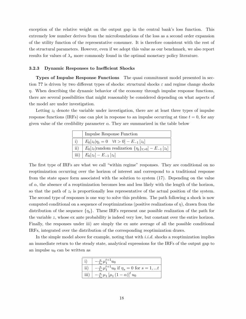
Letting zt denote the variable under investigation, there are at least three types of impulse

response functions (IRFs) one can plot in response to an impulse occurring at time t = 0, for any

given value of the credibility parameter α. They are summarized in the table below

Impulse Response Function

i) E0[zt|ηt = 0 ∀t > 0]−E−1 [zt]ii) E0[zt|random realization ηtt>0]−E−1 [zt]iii) E0[zt]−E−1 [zt]

The first type of IRFs are what we call “within regime” responses. They are conditional on no

reoptimization occurring over the horizon of interest and correspond to a traditional response

from the state space form associated with the solution to system (17). Depending on the value

of α, the absence of a reoptimization becomes less and less likely with the length of the horizon,

so that the path of zt is proportionally less representative of the actual position of the system.

The second type of responses is one way to solve this problem. The path following a shock is now

computed conditional on a sequence of reoptimizations (positive realizations of η), drawn from the

distribution of the sequence ηt. These IRFs represent one possible realization of the path forthe variable z, whose ex ante probability is indeed very low, but constant over the entire horizon.

Finally, the responses under iii) are simply the ex ante average of all the possible conditional

IRFs, integrated over the distribution of the corresponding reoptimization draws.

In the simple model above for example, noting that with i.i.d. shocks a reoptimization implies

an immediate return to the steady state, analytical expressions for the IRFs of the output gap to

an impulse u0 can be written as

i) − κλxµt+11 u0

ii) − κλxµt+11 u0 if ηs = 0 for s = 1, ...t

iii) − κλxµ1 [µ1 (1− α)]t u0

18

Impulse Responses to Independent Shocks With these preliminaries in place we can

now turn to the description of the impulse responses of the simple monetary model presented

in section 3.1 to a unit cost-push shock.18 We assume that the economy starts in steady state,

with zero inflation and no output gap. Since these are also the values of the endogenous variables

that maximize the policymaker’s objective function, changes in regime will not move the economy

away from this steady state as long as cost-push shocks are absent.

Figure 1 shows the path of inflation, output gap and interest rate under commitment and

discretion. With the benchmark calibration, this just replicates the results in Woodford (1999).

Under discretion the central bank moves its instrument with the shock, returning the economy to

steady state as soon as the effects of the shock have faded. Given an i.i.d. impulse, this implies

that the economy is driven into a sharp recession, accompanied by high inflation, but for only

one period. Under commitment instead the central bank exploits the possibility of influencing

inflation expectations in its favor in the period of the shock, by promising a protracted mild

recession, accompanied by deflation. This can be accomplished with a very limited movement in

the interest rate, in the absence of intervening shocks to the natural interest rate. This path for

the policy variable is indeed time inconsistent, since the central bank would want to return to

zero inflation and output gap as soon as the shock has disappeared. Note that this is also the

policy that a new central banker would choose if allowed to reoptimize in any period following

the period of the shock. In fact, in the absence of new shocks, the steady state values of the

endogenous variables are consistent with an optimal commitment.19

What is the behavior of the economy under quasi commitment? Figure 2 provides part of

the answer, presenting IRFs of type i) under two different levels of credibility, associated with an

expected life of the commitment of two quarters and two years respectively. As noted above, this

path for the variables is very unlikely, since it is associated with a string of twenty zero realizations

of the η shock following the cost-push impulse. Nevertheless this experiment is instructive. On the

one hand, we see that the dynamic response of the system is almost indistinguishable from that

under commitment when the average regime duration is α−1 = 8. This suggests that relativelylow levels of credibility are enough to produce qualitative responses of the economy very close to

the ones obtained under commitment. On the other hand, when the expected duration of the

regime is only two quarters, the path of inflation is very close to that under commitment, but

this is associated with a high cost in terms of output. The contraction needed to keep inflation

close to its optimal level is much higher if the central bank has little credibility. This is the path

that would obtain if, at the time of the shock, a new central banker came into office, who refused

to validate the private sector’s expectations and did not reoptimize even in the face of a positive

realization of η. Of course, there is no room in our model for this sort of behavior. The optimal

policy under quasi commitment entails a reoptimization whenever η = 1, and the equilibrium is

18 Impulses are normalized to produce an annualized one percentage point increase in inflation on impact, forgiven expectations. Given the forward looking nature of the model, the actual increase in inflation is a function ofthe forecasted response of policy to the shock.19 This depends from the fact that there is no average inflation bias in our model. The inconsistency of the

optimal plan is thus only conditional on the existence of inefficient shocks.

19

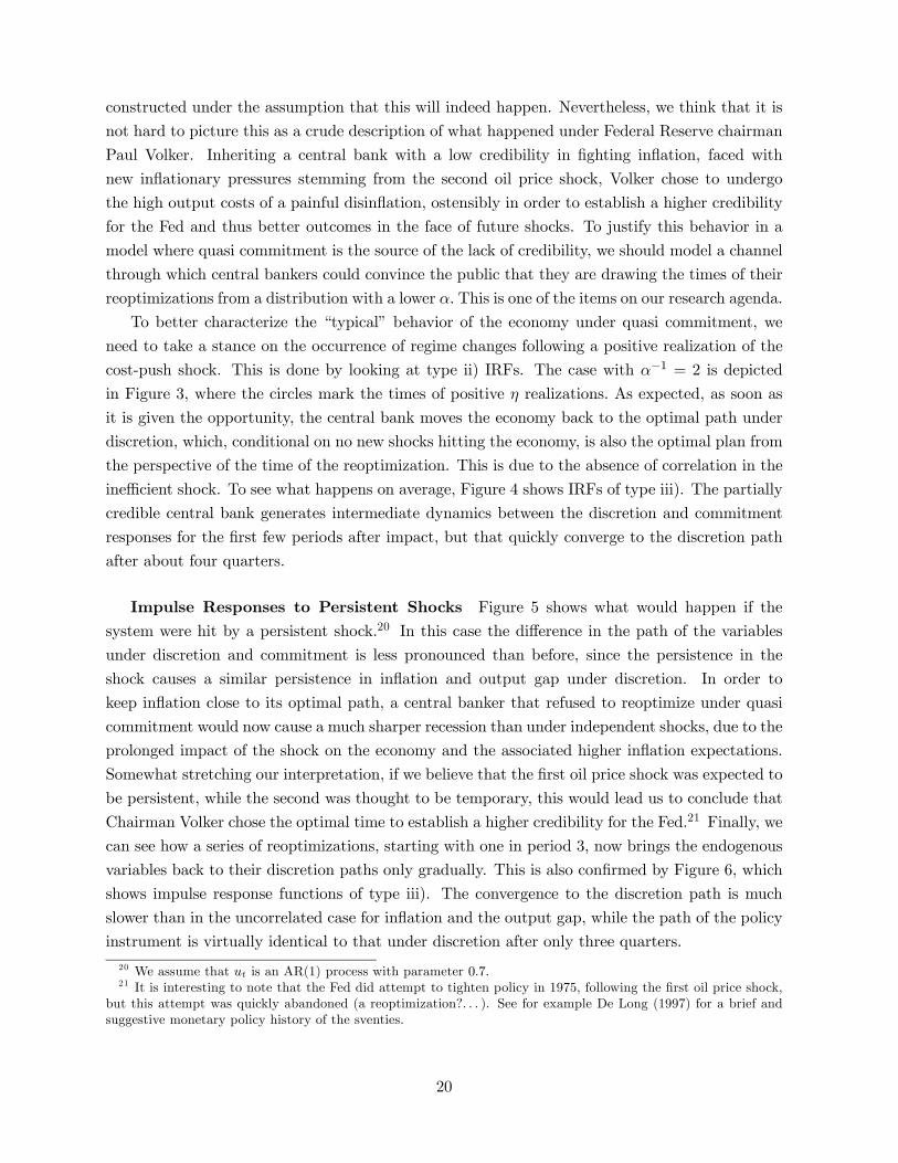
constructed under the assumption that this will indeed happen. Nevertheless, we think that it is

not hard to picture this as a crude description of what happened under Federal Reserve chairman

Paul Volker. Inheriting a central bank with a low credibility in fighting inflation, faced with

new inflationary pressures stemming from the second oil price shock, Volker chose to undergo

the high output costs of a painful disinflation, ostensibly in order to establish a higher credibility

for the Fed and thus better outcomes in the face of future shocks. To justify this behavior in a

model where quasi commitment is the source of the lack of credibility, we should model a channel

through which central bankers could convince the public that they are drawing the times of their

reoptimizations from a distribution with a lower α. This is one of the items on our research agenda.

To better characterize the “typical” behavior of the economy under quasi commitment, we

need to take a stance on the occurrence of regime changes following a positive realization of the

cost-push shock. This is done by looking at type ii) IRFs. The case with α−1 = 2 is depicted

in Figure 3, where the circles mark the times of positive η realizations. As expected, as soon as

it is given the opportunity, the central bank moves the economy back to the optimal path under

discretion, which, conditional on no new shocks hitting the economy, is also the optimal plan from

the perspective of the time of the reoptimization. This is due to the absence of correlation in the

inefficient shock. To see what happens on average, Figure 4 shows IRFs of type iii). The partially

credible central bank generates intermediate dynamics between the discretion and commitment

responses for the first few periods after impact, but that quickly converge to the discretion path

after about four quarters.

Impulse Responses to Persistent Shocks Figure 5 shows what would happen if the

system were hit by a persistent shock.20 In this case the difference in the path of the variables

under discretion and commitment is less pronounced than before, since the persistence in the

shock causes a similar persistence in inflation and output gap under discretion. In order to

keep inflation close to its optimal path, a central banker that refused to reoptimize under quasi

commitment would now cause a much sharper recession than under independent shocks, due to the

prolonged impact of the shock on the economy and the associated higher inflation expectations.

Somewhat stretching our interpretation, if we believe that the first oil price shock was expected to

be persistent, while the second was thought to be temporary, this would lead us to conclude that

Chairman Volker chose the optimal time to establish a higher credibility for the Fed.21 Finally, we

can see how a series of reoptimizations, starting with one in period 3, now brings the endogenous

variables back to their discretion paths only gradually. This is also confirmed by Figure 6, which

shows impulse response functions of type iii). The convergence to the discretion path is much

slower than in the uncorrelated case for inflation and the output gap, while the path of the policy

instrument is virtually identical to that under discretion after only three quarters.

20 We assume that ut is an AR(1) process with parameter 0.7.21 It is interesting to note that the Fed did attempt to tighten policy in 1975, following the first oil price shock,

but this attempt was quickly abandoned (a reoptimization?. . . ). See for example De Long (1997) for a brief andsuggestive monetary policy history of the sventies.

20

Unconditional Moments A very similar picture to the one emerging from the conditional

statements involved in studying impulse response functions also emerges from a look at the un-

conditional second moments of the equilibrium sequences. Figure 7 shows the unconditional

correlations between the endogenous variables, for an economy with i.i.d. shocks. Once again we

see how the ability to commit even for a short number of periods on average has dramatic effects

on the equilibrium behavior of the economy, also contributing to a significant reduction in the

volatility of the policy instrument that is required to achieve the desired equilibrium.

3.3 The Gains from Commitment

So far we have shown that our model’s equilibrium dynamics are significantly influenced by poli-

cymakers’ credibility, and that the continuum of quasi commitment rules bridges the gap between

the commitment and discretion dynamics. Our next step is then to investigate to what extent

credibility influences the level of welfare attainable under the optimal policy, conditional on the

available commitment technology. Before doing this though, it is probably worth commenting on

the metric that we will adopt for these welfare comparisons. If y∗t (α) is the vector of equilibriumvalues for the arguments of the loss function, we can write the expected loss at the beginning of

the planning horizon as L (α) = E [P

t u(y∗t (α))] . Although it is true that any monotonic transfor-

mation of u maintains the same preference ordering, only affine transformations can be consistent

with a given level of the elasticity of substitution. Therefore, for any given calibration, we can

meaningfully interpret the change in welfare associated with different levels of credibility as a

fraction of the total difference in welfare between discretion and commitment. This is the metric

adopted below in our study of the gains from marginal increases in credibility.

Our analysis starts from Figure 8, which shows the effect on the lowest attainable loss of

quarterly increments in the average length of a regime under our benchmark calibration. The

gains from even minimal levels of credibility are very substantial and most of the total gain can

be obtained with an expected duration of the commitment of about three years. More specifically,

as shown in table 1, under the benchmark calibration an average regime length of six quarters

is enough to produce 75% of the gains from commitment, and 90% of the gains can be obtained

by an average duration of the commitment of three and a half years. This strong conclusion is

robust to changes in the relative weight of output in the welfare function, as visually confirmed by

Figure 10, in which inflation and output fluctuations receive the same wight. As shown in Table

1, an average duration of the commitment of nineteen quarters is now required to obtain 75% of

the gains from commitment, but two years are enough to cover half of the gap between discretion

and commitment.

Another instructive way of looking at the significant effect of an even limited amount of

commitment is to plot the combinations of output gap and inflation volatility associated with the

optimal policy for different levels of α. Figure 9 shows an even starker picture than the welfare

comparisons. A commitment expected to last for only two quarters cuts the volatility of inflation

by more than one half, with no discernible effect on the volatility of the output gap. An average

21

duration of the commitment of one year is enough to move within two basis points of the inflation

volatility under commitment, again with no significant losses in terms of output stabilization.

Of course, further reductions in the volatility of inflation require significantly bigger sacrifices

in terms of output volatility. In comparison, the volatility frontier in Figure 11 shows a much

smoother transition from discretion to commitment in the case of λx = 1, consistent with the

corresponding results of the welfare ranking.

Finally, to illustrate the effect of credibility across all choices of output weights, Figure 12

displays the efficient frontiers traced out by letting λx vary from our low benchmark value to

infinity, with each line corresponding to a specific credibility level α. Note that, as λx increases

towards infinity, all the curves converge to (1, 0) in sd(π)−sd(x) space, since in this case, regardlessof the level of α, output is completely stabilized and the cost-push shocks feed directly into the

inflation rate. What is interesting however is that, quite uniformly across output weights, we

observe substantial welfare gains from marginal increases in credibility at low levels of expected

regime duration.

4 Conclusion

This paper introduced the notion of quasi commitment, a policy rule with limited commitment in

which policymakers renege on their announced optimal plans with a constant, exogenous proba-

bility every period. In this framework, commitment and discretion become the two polar cases of

a more general decision making procedure. Assuming that private agents know the probability of

a renegotiation, and form expectations on the future course of policy accordingly, we can interpret

the expected duration of the announced plans as a continuous measure of whether policymakers

match deeds to words. This is the notion of credibility proposed by Blinder (1998). We then

apply our solution method to a calibrated version of a forward looking model of the monetary

transmission mechanism. Our results confirm that, even in the absence of any reason for the cen-

tral bank to induce a bias in the average level of inflation, commitment is superior to discretion

in the natural metric of a second order approximation to the utility of the representative agent.

More interestingly, we find that most of the gains from commitment accrue at relatively low levels

of credibility. In our benchmark calibration, a commitment expected to last for six quarters is

enough to bridge 75% of the welfare gap between discretion and commitment. We also show that

this result is robust to variations in the welfare weight on output gap fluctuations.

This paper is only a preliminary study of the behavior of a particular model economy under

quasi commitment. The robustness of our results across different models of the monetary trans-

mission mechanism is an open question, that warrants further investigation. In fact, progress in

this direction can be accomplished with a relatively modest effort, given that our solution method

has been devised for a general class of DSGE models that admit a log-linear representation as an

expectational VAR system.

Finally, endogenizing the probability of a change in regime seems an obvious step to increase

the empirical plausibility of the model. We could think of two ways of accomplishing this, which

22

we see as complementary. On the one hand, we could allow central bankers to invest in their

credibility, for example by refusing to reoptimize when given the option. This would indeed be

justified only as long as the private sector could learn about the new frequency of reoptimizations.

Comparing the costs of the transition, when inflation expectations are higher than what is justified

by the actual behavior of the central bank, with the long run gains associated with the higher level

of credibility, would produce a normative analysis of the transition from low to high credibility

regimes. On the other hand, and more in the spirit of Flood and Isard (1988), we could assume

that the probability of a reoptimization depends on the state of the economy, for example by

making this probability a function of the vector of predetermined Lagrange multipliers, which

measure the temptation to disregard the associated constraints and reoptimize. Even though

arguably desirable on the grounds of realism, these extensions would come at the cost of foregoing

the linear quadratic structure that provides the model its extreme tractability. For this reason we

think that the quasi commitment framework with exogenous reoptimizations provides a useful first

step in the direction of expanding the menu of policy rules besides discretion and commitment.

23

A Some Details of the Calculations

Below we provide a few additional details of the solution. A fully worked out set of calculations

is available from the authors upon request.

A.1 From the Bellman Equation to the Lagrangian

The recursive formulation of the policymaker’s problem stated regime by regime is given in (6) as

V (xτj ) = minxk,Xk,ik∞k=0

maxϕk∞k=0

Eτj

∆τjXk=0

βk£Lτj+k + β∆τj+1V (xτj+1) (21)

+2ϕ0τj+k+1³GEτj+kXτj+k+1

−A21xτj+k −A22Xτj+k−B2iτj+k

´ios.t.

xτj+k+1 −A11xτj+k −A12Xτj+k−B1iτj+k − ετj+k+1 = 0

ϕτj = 0

The policymaker calculates the first order condition of (21) taking as given private agents’

rational expectation formation

Eτj+k [Xτj+k+1] = (1− α)Eτj+k [Xτj+k+1|τ j+1 > τ j + k + 1] + αHEτj+k[xτj+k+1] (22)

as well as the form of the value function

V (x) = x0Px+ ρ (23)

The running cost function in (21) involves a random sum since the policymaker is uncertain

about how many periods the current regime will last. Thus she must take into account that the

regime will last for any given number of periods with positive probability. In this context, the

assumed exogeneity of the regime change signals represents a major simplification. In particular,

the assumption implies that ∀j : ∆τ j ∼Geometric(α), so that Pr∆τ = m = (1− α)mα.

Using the law of iterated expectations we can apply Eτj+k[·|τ j = m] to the kth term in (21),

where k ≤ m. Note that

Eτj+k[ϕ0τj+k+1

Eτj+kXτj+k+1|∆τ j = m] = ϕ0τj+k+1Eτj+kXτj+k+1

Eτj [β∆τ+1V (xτj+1)|∆τ j = m] = βm+1EτjV (xτj+m+1)

and that (22) and (23) may be substituted on the right hand side of (21). Finally, noting that

Eτj [·] =∞X

m=0

α(1− α)mEτj [·|∆τ j = m]

and switching the sums over k and m, one obtains the Lagrangian corresponding to (21)

24

L = Eτj

( ∞Xm=0

(β(1− α))mhLτj+m + αβ

³x0τj+m+1P xτj+m+1 + ρ

´(24)

+2ϕ0τj+m+1¡(1− α)GEτj+m

£Xτj+m+1

¯∆τ j > m+ 1

¤+αGHxτj+m+1 −A21xτj+m −A22Xτj+m −B2iτj+m

¢+2φ0τj+m+1(xτj+1+m −A11xτj+m −A12Xτj+m −B1iτj+m)

ioA.2 Solving for the Value Function

After solving the first order conditions of the Lagrangian (24), one may solve for the value function

parameters (P, ρ) by substituting the state space representation of the equilibrium dynamics

(10) into the Bellman equation (6). Collecting quadratic terms in the state variables yields an

expression for P

P =

µInx×nx0nX×nx

¶0V1

µInx×nx0nX×nx

¶+ αβ

µInx×nx0nX×nx

¶0M 0V2M

µInx×nx0nX×nx

¶where the matrices V1, V2 solve the Sylvester equations

V1 =

Inx×nx 0nx×nXC

ξ0

0

W

Inx×nx 0nx×nXC

ξ0

+ β(1− α)M 0V1M

V2 =

µInx×nx0nX×nx

¶P

µInx×nx0nX×nx

¶0+ β(1− α)M 0V2M

Similarly, collecting constant terms yields an expression for ρ

ρ =β

1− β

µ(1− α)tr

µInx×nx0nX×nx

¶0V1

µInx×nx0nX×nx

¶Ω¶

+αtrµInx×nx0nX×nx

¶0V2

µInx×nx0nX×nx

¶Ω

Note that the matrices V1, V2 are functions of the state space form M,C, ξ alone. Interestingly,one immediately retrieves the value function of the discretion problem by setting α = 1 (see for

instance Söderlind, 1999). When α = 0 instead, the value function reduces to a Sylvester equation

whose solution is the expected discounted sum of period losses conditional on the state space form

holding forever.

25

References

Abreu, Dilip, D. Pierce and E. Stacchetti (1986), “Optimal Cartel Equilibria with Imperfect

Monitoring,” Journal of Economic Theory 39:251—269.

Abreu, Dilip, D. Pierce and E. Stacchetti (1990), “Toward a Theory of Discounted Repeated

Games with Imperfect Monitoring,” Econometrica 58:1041—1063.

Barro, Robert J. and D.B. Gordon (1983), “A Positive Theory of Monetary Policy in a Natural

Rate Model,” Journal of Political Economy 91:589—610.

Barro, Robert J (1986), “Reputation in a Model of Monetary Policy with Incomplete Information”

Journal of Monetary Economics 17: 3—20.

Blackburn, Keith and Michael Christensen (1989), “Monetary Policy and Policy Credibility: The-

ories and Evidence” Journal of Economic Literature 27: 1—45.

Blinder, Alan S. (1998), Central Banking in Theory and Practice, Cambridge, MA: MIT Press.

Calvo, Guillermo A. (1978), “On the Time Consistency of Optimal Policy in a Monetary Econ-

omy,” Econometrica 46:1411—1428.

Kara, A. Hakan (2002), “Optimal Monetary Policy Rules under Imperfect Commitment,” mimeo,

New York University.

Chari V.V. and P. Kehoe (1990), “Sustainable Plans,” Journal of Political Economy 98:783—802.

Clarida, Richard, Jordi Galí and Mark Gertler (1999), “The Science of Monetary Policy: A New

Keynesian Perspective” Journal of Economic Literature 37: 1661—1707.

Cukierman, Alex (1992), Central Bank Strategy, Credibility, and Independence: Theory and Evi-

dence, Cambridge: MIT Press.

Cukierman, Alex, Steven B. Webb and Bilin Neyapti (1992), “Measuring the Independence of

Central Banks and Its Effect on Policy Outcomes” World Bank Economic Review 6:353-398.

DeLong, Bradford J. (1997),“America’s Peacetime Inflation: The 1970s” in Christina Romer and

David Romer (eds.) Reducing Inflation: Motivation and Strategy, Chicago: University of Chicago

Press.

Faust, Jon and Lars E.O. Svensson (2000), “Transparency and Credibility: Monetary Policy with

Unobservable Goals,” International Economic Review 42:369—397.

Fischer, Stanley (1980), “Dynamic Inconsistency, Cooperation and the Benevolent Dissembling

Government,” Journal of Economic Dynamics and Control 2:93—107.

Flood and Isard (1988), “Monetary Policy Strategies,” NBER Working Paper No. 2770.

Galí, Jordi (2001), “New Perspectives on Monetary Policy, Inflation, and the Business Cycle”, in

M. Dewatripont, L. Hansen and S. Turnovsky (eds.) Advances in Economics and Econometrics,

the Eight World Congress, Cambridge, UK: Cambridge University Press.

26

Kydland, Finn E. and Edward C. Prescott (1977), “Rules Rather than Discretion: The Inconsis-

tency of Optimal Plans” Journal of Political Economy 85: 473—491.

Ljungquist, Lars and T. Sargent (2000), Recursive Macroeconomics Theory, Boston: MIT Press

Marcet, Albert and Ramon Marimon (1999), “Recursive Contracts” mimeo, Universitat Pompeu

Fabra

McCallum, Bennett T. (1999), “Issues in the Design of Monetary Policy Rules” in J.B. Taylor

and M. Woodford (eds.) Handbook of Macroeconomics, Amsterdam: North-Holland.

Phelan, Christopher (2001), “Public Trust and Government Betrayal,” mimeo, Federal Reserve

Bank of Minneapolis.

Phelan, Christopher and E. Stacchetti (2001), “Sequential Equilibria in a Ramsey Tax Model,”

Econometrica 69:1491—1518.

Roberds, William (1987), “Models of Policy Under Stochastic Replanning,” International Eco-

nomic Review, 28:731—755.

Rogoff, Kenneth (1985), “The Optimal Degree of Commitment to a Monetary Target,” Quarterly

Journal of Economics 100:1169—1190

Rogoff (1989) “Reputation, Coordination and Monetary Policy” in Robert J. Barro (ed.) Modern

Business Cycle Theory, Cambridge, MA: Harvard University Press.

Söderlind, Paul (1999), “Solution and Estimation of RE Macromodels with Optimal Policy,”

European Economic Review 41:111—1146.

Stokey, Nancy (1989), “Reputation and Time Consistency,” American Economic Review 79:134—

139.

Stokey, Nancy (1991), “Credible Public Policy,” Journal of Economic Dynamics and Control

15:627—657.

Svensson, Lars E.O. (1999a), “Inflation Targeting as a Monetary Policy Rule”, Journal of Mone-

tary Economics 43: 607-654.

Svensson, Lars E. O. (1999b), “How Should Monetary Policy Be Conducted in an Era of Price

Stability?” inNew Challenges for Monetary Policy, a symposium sponsored by the Federal Reserve

Bank of Kansas City.

Svensson, Lars E.O.and Michael D. Woodford (2003), “Implementing Optimal Policy through

Inflation-Forecast Targeting,” in Bernanke, Ben S. and Michael Woodford (eds.) Inflation Tar-

geting, Chicago: University of Chicago Press.

Woodford, Michael D. (1999), “Commentary: How Should Monetary Policy Be Conducted in an

Era of Price Stability?”in New Challenges for Monetary Policy, a symposium sponsored by the

Federal Reserve Bank of Kansas City.

Woodford, Michael D. (2003), Interest and Prices: Foundations of a Theory of Monetary Policy,

Princeton: Princeton University Press.

27

Figures and Tables

0 2 4 6 8 10 12 14 16 18 20-0.5

0

0.5

1

πt reaction to u

t shock

0 2 4 6 8 10 12 14 16 18 20-2

-1.5

-1

-0.5

0

xt reaction to u

t shock

0 2 4 6 8 10 12 14 16 18 200

0.5

1

1.5

it reaction to u

t shock

Figure 1: Dynamic responses to a one standard deviation, uncorrelated cost push shock under commitmentand discretion. The fat dotted lines are the discretion responses and the fat dashed lines are the commitment

responses. The weight on output in the loss function is λx = 0.05.

28

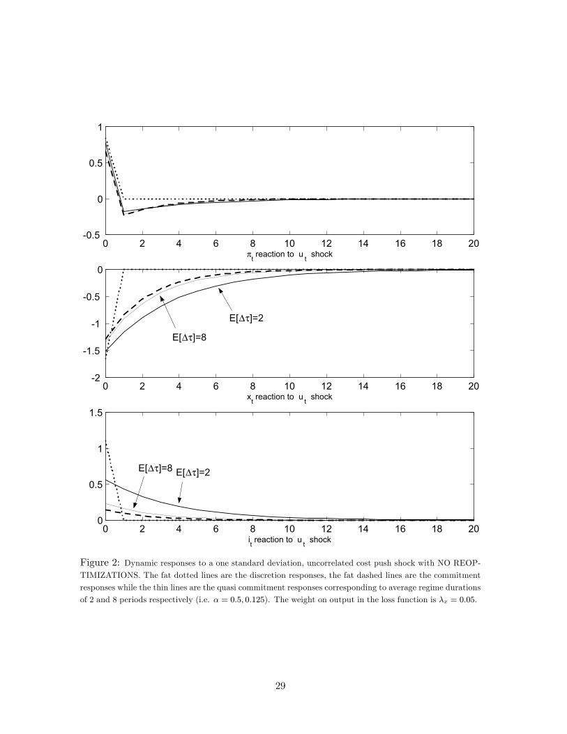
0 2 4 6 8 10 12 14 16 18 20-0.5

0

0.5

1

πt reaction to u t shock

0 2 4 6 8 10 12 14 16 18 20-2

-1.5

-1

-0.5

0

xt reaction to u t shock

0 2 4 6 8 10 12 14 16 18 200

0.5

1

1.5

it reaction to u t shock

E[∆τ]=2

E[∆τ]=8

E[∆τ]=8 E[∆τ]=2

Figure 2: Dynamic responses to a one standard deviation, uncorrelated cost push shock with NO REOP-

TIMIZATIONS. The fat dotted lines are the discretion responses, the fat dashed lines are the commitment

responses while the thin lines are the quasi commitment responses corresponding to average regime durations

of 2 and 8 periods respectively (i.e. α = 0.5, 0.125). The weight on output in the loss function is λx = 0.05.

29

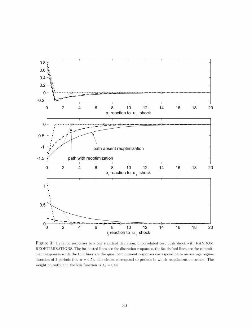
0 2 4 6 8 10 12 14 16 18 20

-0.2

0

0.2

0.4

0.6

0.8

πt reaction to u

t shock

0 2 4 6 8 10 12 14 16 18 20

-1.5

-1

-0.5

0

xt reaction to u

t shock

0 2 4 6 8 10 12 14 16 18 200

0.5

1

it reaction to u

t shock

path absent reoptimization

path with reoptimization

Figure 3: Dynamic responses to a one standard deviation, uncorrelated cost push shock with RANDOMREOPTIMIZATIONS. The fat dotted lines are the discretion responses, the fat dashed lines are the commit-

ment responses while the thin lines are the quasi commitment responses corresponding to an average regime

duration of 2 periods (i.e. α = 0.5). The circles correspond to periods in which reoptimization occurs. The

weight on output in the loss function is λx = 0.05.

30

0 2 4 6 8 10 12 14 16 18 20

-0.2

0

0.2

0.4

0.6

0.8

πt reaction to u

t shock

0 2 4 6 8 10 12 14 16 18 20

-1.5

-1

-0.5

0

xt reaction to u

t shock

0 2 4 6 8 10 12 14 16 18 200

0.25

0.5

0.75

1

it reaction to u

t shock

average response when E[ ∆τ]=2

Figure 4: Dynamic responses to a one standard deviation, uncorrelated cost push shock, AVERAGINGOVER REGIME CHANGES. The fat dotted lines are the discretion responses, the fat dashed lines are the

commitment responses while the continuous lines are the average quasi commitment responses corresponding

to an average regime duration of 2 periods (i.e. α = 0.5). The weight on output in the loss function is

λx = 0.05 .

31

0 2 4 6 8 10 12 14 16 18 20-0.5

0

0.5

1

1.5

2

πt reaction to u

t shock

0 2 4 6 8 10 12 14 16 18 20-6

-4

-2

0

xt reaction to u

t shock

0 2 4 6 8 10 12 14 16 18 20-0.5

0

0.5

1

1.5

2

it reaction to u

t shock

path absent reoptimization

path with reoptimization

Figure 5: Dynamic responses to a one standard deviation, serially correlated (ρu = 0.7) cost push shock

with RANDOM REOPTIMIZATIONS. The fat dotted lines are the discretion responses, the fat dashed

lines are the commitment responses while the thin lines are the quasi commitment responses corresponding

to an average regime duration of 2 periods (i.e. α = 0.5). The circles correspond to periods in which

reoptimization occurs. The weight on output in the loss function is λx = 0.05 .

32

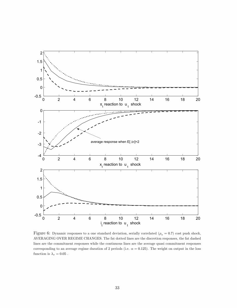
0 2 4 6 8 10 12 14 16 18 20-0.5

0

0.5

1

1.5

2

πt reaction to u

t shock

0 2 4 6 8 10 12 14 16 18 20-4

-3

-2

-1

0

xt reaction to u

t shock

0 2 4 6 8 10 12 14 16 18 20-0.5

0

0.5

1

1.5

2

it reaction to u

t shock

average response when E[ ∆τ]=2

Figure 6: Dynamic responses to a one standard deviation, serially correlated (ρu = 0.7) cost push shock,AVERAGING OVER REGIME CHANGES. The fat dotted lines are the discretion responses, the fat dashed

lines are the commitment responses while the continuous lines are the average quasi commitment responses

corresponding to an average regime duration of 2 periods (i.e. α = 0.125). The weight on output in the loss

function is λx = 0.05 .

33

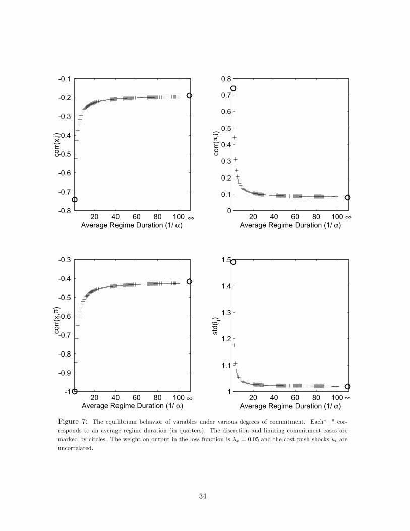
20 40 60 80 100-0.8

-0.7

-0.6

-0.5

-0.4

-0.3

-0.2

-0.1

Average Regime Duration (1/ α)

corr(

x,i)

20 40 60 80 1000

0.1

0.2

0.3

0.4

0.5

0.6

0.7

0.8

Average Regime Duration (1/ α)co

rr(π ,

i)

20 40 60 80 100-1

-0.9

-0.8

-0.7

-0.6

-0.5

-0.4

-0.3

Average Regime Duration (1/ α)

corr(

x,π )

20 40 60 80 1001

1.1

1.2

1.3

1.4

1.5

Average Regime Duration (1/ α)

std(

i t)∞ ∞

∞ ∞

Figure 7: The equilibrium behavior of variables under various degrees of commitment. Each“+" cor-

responds to an average regime duration (in quarters). The discretion and limiting commitment cases are

marked by circles. The weight on output in the loss function is λx = 0.05 and the cost push shocks ut are

uncorrelated.

34

10 20 30 40 50 60 70 80 90 10065

70

75

80

85

Average Regime Duration (1/ α)

E[L]

discretion

commitment

Figure 8: The gains from credibility. Each“+" corresponds to an average regimeduration (in quarters). The limiting cases of discretion and commitment are

marked by circles. The weight on output is λx = 0.05 and the cost push shocks

ut are uncorrelated.

0.7 0.72 0.74 0.76 0.78 0.8 0.82 0.84 0.861.65

1.66

1.67

1.68

1.69

1.7

1.71

1.72

std π

std

x

commitment

discretion

Figure 9: The efficient frontier as a function of the average credibility. Each“+" cor-responds to an average regime duration (in quarters). The limiting cases of discretion

and commitment are marked by circles. The weight on output is λx = 0.05 and the

cost push shocks ut are uncorrelated.

35

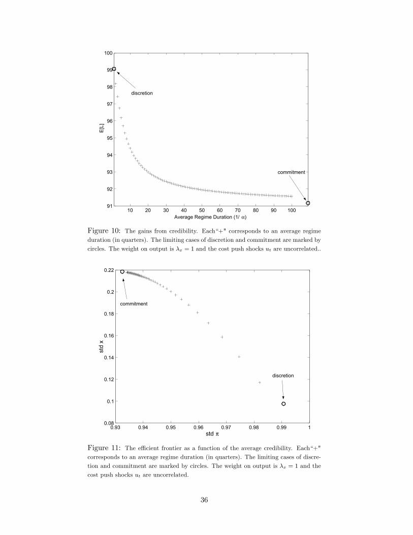
10 20 30 40 50 60 70 80 90 10091

92

93

94

95

96

97

98

99

100

Average Regime Duration (1/ α)

E[L]

discretion

commitment

Figure 10: The gains from credibility. Each“+" corresponds to an average regime

duration (in quarters). The limiting cases of discretion and commitment are marked by

circles. The weight on output is λx = 1 and the cost push shocks ut are uncorrelated..

0.93 0.94 0.95 0.96 0.97 0.98 0.99 10.08

0.1

0.12

0.14

0.16

0.18

0.2

0.22

std π

std

x

commitment

discretion

Figure 11: The efficient frontier as a function of the average credibility. Each“+"corresponds to an average regime duration (in quarters). The limiting cases of discre-

tion and commitment are marked by circles. The weight on output is λx = 1 and the

cost push shocks ut are uncorrelated.

36

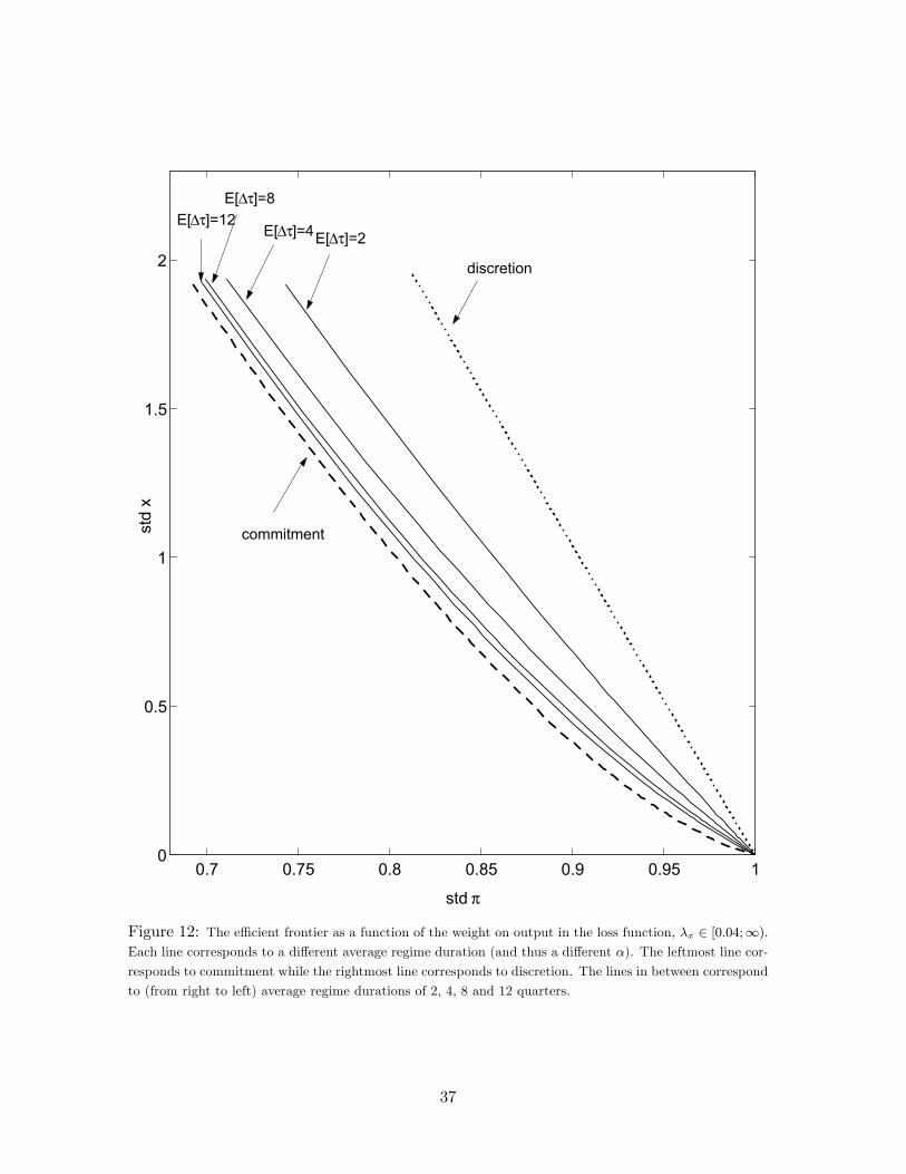
0.7 0.75 0.8 0.85 0.9 0.95 10

0.5

1

1.5

2

std π

std

x

E[∆τ]=12 E[∆τ]=8

E[∆τ]=4 E[∆τ]=2

discretion

commitment

Figure 12: The efficient frontier as a function of the weight on output in the loss function, λx ∈ [0.04;∞).Each line corresponds to a different average regime duration (and thus a different α). The leftmost line cor-

responds to commitment while the rightmost line corresponds to discretion. The lines in between correspond

to (from right to left) average regime durations of 2, 4, 8 and 12 quarters.

37

Weight on Output: λx

G

a

i

n

0.05 0.25 0.50 1.00

25% 2(39%)

3(37%)

3(28%)

4(29%)

50% 3(57%)

5(56%)

6(52%)

8(52%)

75% 6(78%)

10(76%)

14(76%)

19(76%)

90% 14(90%)

26(90%)

36(90%)

50(90%)

Table 1: The table entries show how many periods the central bank needs to

commit for, on average, in order to achive at least some given percentage of

the total gain from commitment. The numbers in paranthesis are the actual

percentage gains. They differ because only integer (average) commitment lengths

are considered.

38