1

COMP4971C Independent Work (Spring, 2018/2019)

Momentum Trading in Hong Kong Stock Market

Kwok Tsz Hong

Supervisor:

Prof. David Rossiter

2

Content

Introduction .................................................................................................................... 4

Software Framework and Data ...................................................................................... 4

Overview ........................................................................................................................ 4

1. Methodology ........................................................................................................... 6

1.1. Selection of stock ...................................................................................................... 6

1.2. Stock Data used in the study ..................................................................................... 6

1.3. Trading Strategy ........................................................................................................ 7

1.3.1. Steps to calculate the equity .............................................................................. 9

2. Optimization ......................................................................................................... 10

2.1. Measurements ............................................................................................................ 10

2.1.1. Compound Annual Growth Rate (CAGR) ......................................................... 10

2.1.2. Maximum Draw Down (MDD) ....................................................................... 10

2.1.3. Sharpe Ratio .................................................................................................... 10

2.2. Result ....................................................................................................................... 11

3. Additional constraints ........................................................................................... 15

3.1. SMA of the HSI ......................................................................................................... 15

3.2. SMA of individual stock ........................................................................................... 16

3.3. Z-score of individual stock ........................................................................................ 17

3.4. MACD of HSI ......................................................................................................... 19

3.5. MACD of individual stock ...................................................................................... 20

3.6. Comparison ............................................................................................................. 21

4. Testing .................................................................................................................. 22

4.1. Testing results ............................................................................................................ 22

4.1.1. Original ............................................................................................................... 23

4.1.2. SMA of HSI ........................................................................................................ 24

4.1.3. SMA of stock ...................................................................................................... 25

4.1.4. Z-score ................................................................................................................ 26

4.1.5. MACD of HSI .................................................................................................... 27

4.1.6. MACD of stock .................................................................................................. 28

3

4.2. Comparison .................................................................................................................. 29

5. Conclusion ............................................................................................................ 30

6. Discussion ............................................................................................................. 31

4

Introduction

In this study, momentum trading strategies is used in Hong Kong stock market.

Hong Kong stock market has total number 13,869 of listed securities. Listed companies

are from all over the world, which included Hong Kong, mainland China, Taiwan,

United States, etc. Upward momentum trading strategy is mainly used in this study,

with additional indicators as auxiliary. Our target is to have a higher return comparing

with the Hang Seng Index and beat the inflation, with a simple rule indicated by the

momentum.

Software Framework and Data

Hong Kong historical data is download from Yahoo finance. In this report, Jupyter

notebook with Python 3.6.3 is used in this project. The program is developed based on

libraries:

pandas, for data management.

matplotlib, for data visualization.

numpy, for mathematics computation.

Overview

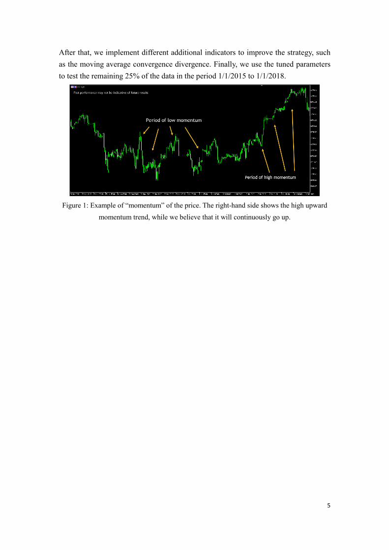
Momentum trading is aimed to capture the trend, either upward or downward,

example of momentum is shown in figure 1. In this study, we believe that if the stock

price is moving in one direction (either going up, or down), it would be likely to

continuously move in the same direction. In this study, we only focus on the upward

trend, which is the increasing trend. Since the downward trend requires us to sell the

stock. If the stock in increasing while we are selling it, then there is a chance that we

will lose all the money. So, we believe that the selling process required more work on

stopping the loss. Therefore, in the preliminary state, we only focus on the upward trend.

To determine the trend, we use long-term (in unit of day) percent change and short-term

(in unit of day) percent change. After buying the stock, we will hold it for a fixed period.

Then, we will optimize these three parameters, which are the days of the long-term

percent change, days of the short-term percent change and the days for holding the stock,

by using the around 75% of the past historical data, which is from 1/1/2005 to 1/1/2015.

5

After that, we implement different additional indicators to improve the strategy, such

as the moving average convergence divergence. Finally, we use the tuned parameters

to test the remaining 25% of the data in the period 1/1/2015 to 1/1/2018.

Figure 1: Example of “momentum” of the price. The right-hand side shows the high upward

momentum trend, while we believe that it will continuously go up.

6

1. Methodology

We split the data into training and testing sets by the ratio around 75/25. To test

our strategy, the period 1/1/2005 to 1/1/2015 (around 75%) is selected to optimize the

parameters. Then, we will use the period 1/1/2015 to 1/1/2018 (around 25%) to quantify

the performance of our strategy.

1.1. Selection of stock

There are 75 valid stocks are selected by the following rules:

1. Setting the average daily volume limit to be 1,000,000: The stocks with average

daily volume larger than the limit will be selected.

2. Stock is listed within the period: Since there are some stocks that was closed

during the period, and some had not yet in the list during the period. We will drop

all those stocks for simplicity.

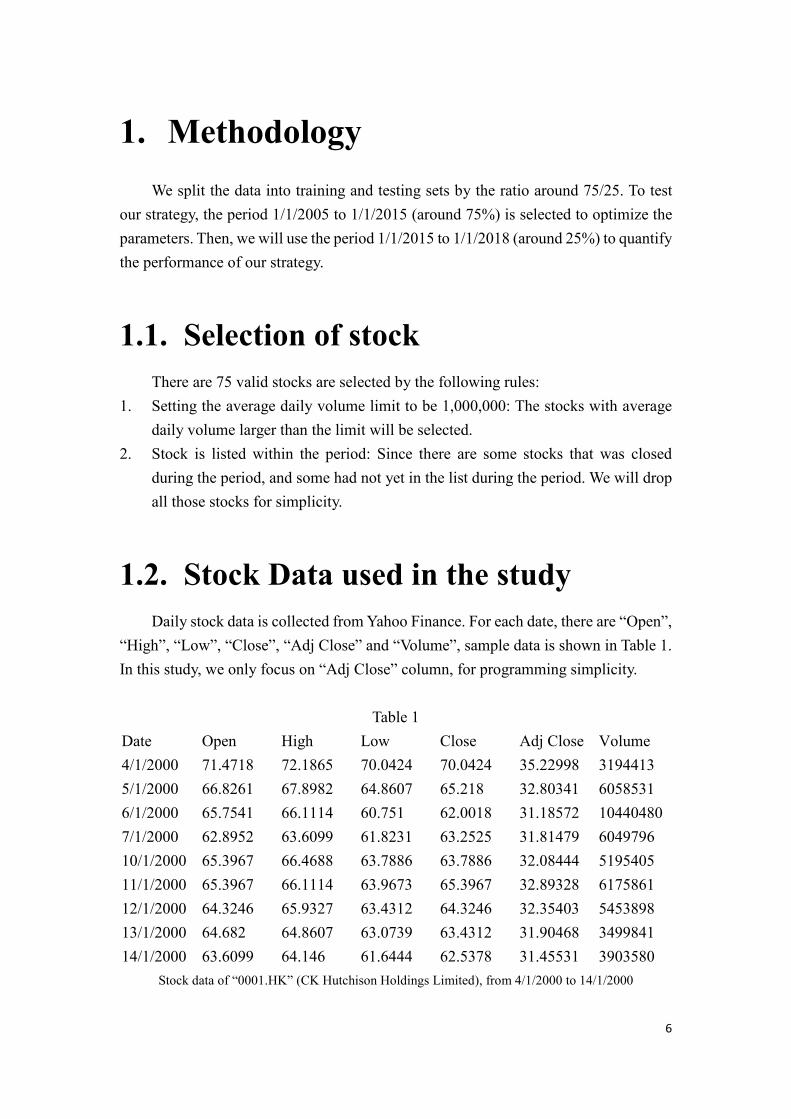
1.2. Stock Data used in the study

Daily stock data is collected from Yahoo Finance. For each date, there are “Open”,

“High”, “Low”, “Close”, “Adj Close” and “Volume”, sample data is shown in Table 1.

In this study, we only focus on “Adj Close” column, for programming simplicity.

Table 1

Date Open High Low Close Adj Close Volume

4/1/2000 71.4718 72.1865 70.0424 70.0424 35.22998 3194413

5/1/2000 66.8261 67.8982 64.8607 65.218 32.80341 6058531

6/1/2000 65.7541 66.1114 60.751 62.0018 31.18572 10440480

7/1/2000 62.8952 63.6099 61.8231 63.2525 31.81479 6049796

10/1/2000 65.3967 66.4688 63.7886 63.7886 32.08444 5195405

11/1/2000 65.3967 66.1114 63.9673 65.3967 32.89328 6175861

12/1/2000 64.3246 65.9327 63.4312 64.3246 32.35403 5453898

13/1/2000 64.682 64.8607 63.0739 63.4312 31.90468 3499841

14/1/2000 63.6099 64.146 61.6444 62.5378 31.45531 3903580

Stock data of “0001.HK” (CK Hutchison Holdings Limited), from 4/1/2000 to 14/1/2000

7

1.3. Trading Strategy

In order to find out the momentum of the stock price, we assign two parameters to

determine the trend. They are the �� days Percent Change ��(��) and �� days

Percent Change ��(��) . ��(��) indicates the relatively long-term trend, while ��(��) indicates the relatively short-term trend ( �� > �� ). Buy signal will be

generated if it is determined as upward momentum, which means the increasing trend.

Sign of the momentum at time T is defined by:

(�) = > 0, ��(��) > 0 and ��(��) > 0< 0, ��(��) < 0 and ��(��) < 0= 0, ��ℎ������ ,

where ��(�) = �� � ��� �� × 100%, $% is the price at time T, $%�& is the price at

time � − �, which means � days ago.

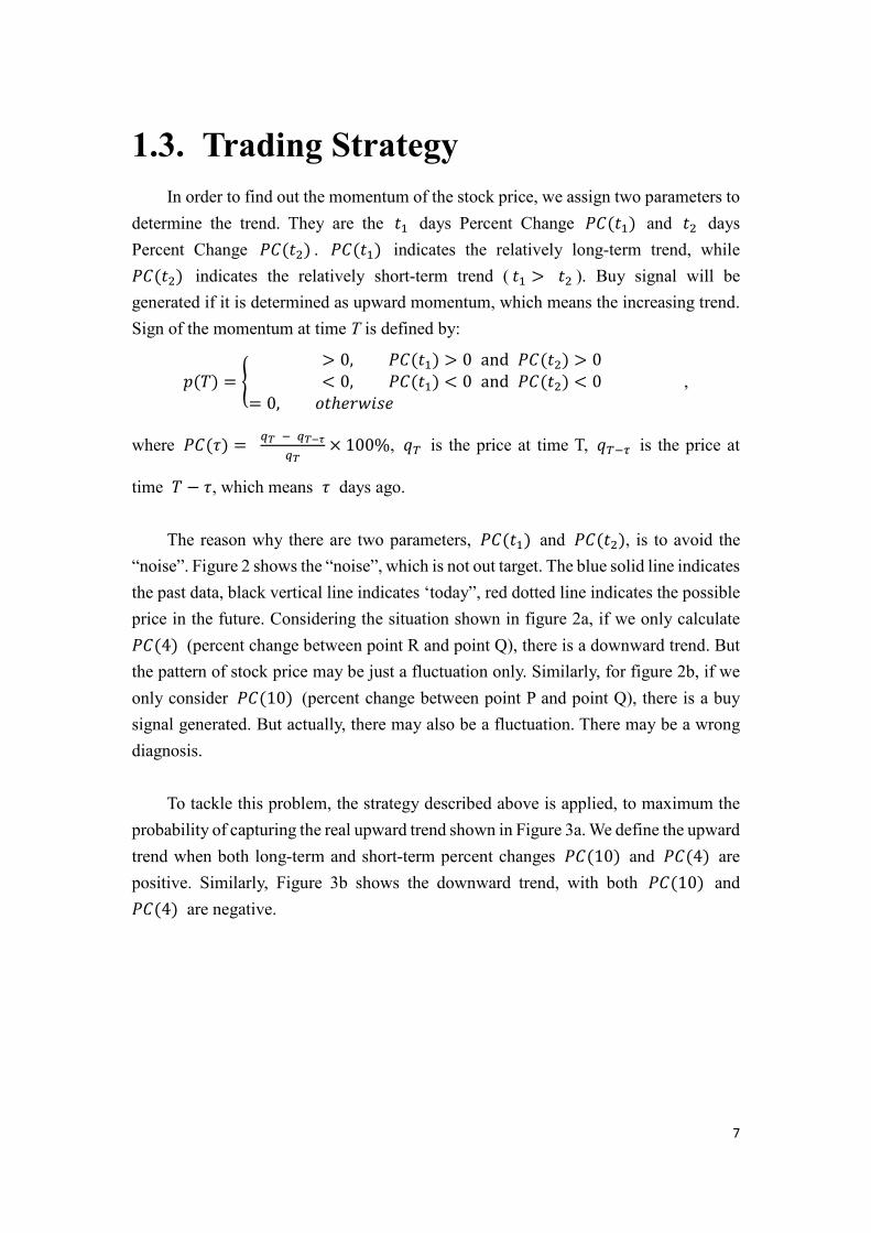
The reason why there are two parameters, ��(��) and ��(��), is to avoid the

“noise”. Figure 2 shows the “noise”, which is not out target. The blue solid line indicates

the past data, black vertical line indicates ‘today”, red dotted line indicates the possible

price in the future. Considering the situation shown in figure 2a, if we only calculate ��(4) (percent change between point R and point Q), there is a downward trend. But

the pattern of stock price may be just a fluctuation only. Similarly, for figure 2b, if we

only consider ��(10) (percent change between point P and point Q), there is a buy

signal generated. But actually, there may also be a fluctuation. There may be a wrong

diagnosis.

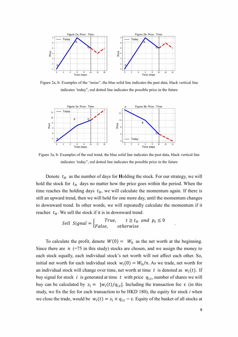
To tackle this problem, the strategy described above is applied, to maximum the

probability of capturing the real upward trend shown in Figure 3a. We define the upward

trend when both long-term and short-term percent changes ��(10) and ��(4) are

positive. Similarly, Figure 3b shows the downward trend, with both ��(10) and ��(4) are negative.

8

Figure 2a, b: Examples of the “noise”, the blue solid line indicates the past data, black vertical line

indicates ‘today”, red dotted line indicates the possible price in the future

Figure 3a, b: Examples of the real trend, the blue solid line indicates the past data, black vertical line

indicates ‘today”, red dotted line indicates the possible price in the future

Denote �) as the number of days for Holding the stock. For our strategy, we will

hold the stock for �) days no matter how the price goes within the period. When the

time reaches the holding days �), we will calculate the momentum again. If there is

still an upward trend, then we will hold for one more day, until the momentum changes

to downward trend. In other words, we will repeatedly calculate the momentum if it

reaches �). We sell the stock if it is in downward trend.

*�++ *�,-.+ = / ��0�, � 1 �) .-2 3 4 05.+��, ��ℎ������ .

To calculate the profit, denote 6(0) = 67 as the net worth at the beginning.

Since there are - (=75 in this study) stocks are chosen, and we assign the money to

each stock equally, each individual stock’s net worth will not affect each other. So,

initial net worth for each individual stock �8(0) = 67/-. As we trade, net worth for

an individual stock will change over time, net worth at time � is denoted as �8(�). If

buy signal for stock � is generated at time � with price $8,3, number of shares we will

buy can be calculated by �8 = ⌊�8(�)/$8,3⌋. Including the transaction fee ε (in this

study, we fix the fee for each transaction to be HKD 180), the equity for stock i when

we close the trade, would be �8(�) = �8 × $8,3 − ε. Equity of the basket of all stocks at

9

time � can be calculated by 6(�) = ∑ �8,38 = ∑ (�8 × $8,3 + @8,3)8 , where ∑ @8,38 is the

cash remained at time t.

1.3.1. Steps to calculate the equity

1 Select the stocks according to the section “Selection of stock”.

2 Equally assign the money to each stock and treat each of them as an individual

system. In other words, they will not affect each other.

3 Buy as many as shares if a buy signal is generated for an individual stock.

4 Sum the net worth and the remaining cash of each stock to calculate the whole net

worth of our portfolio.

10

2. Optimization

2.1. Measurements

2.1.1. Compound Annual Growth Rate (CAGR)

“The rate of return that would be required for an investment to grow from its

beginning balance to its ending balance, assuming the profits were reinvested at the end

of each year of the investment’s lifespan” (Investopedia, 2019).

�ABC = (DEEE)FG − 1,

where EB is the ending balance, BB is the beginning balance, n is the number of

years.

2.1.2. Maximum Draw Down (MDD)

“The Maximum loss from a peak to a trough of a portfolio, before a new peak is

attained” (Investopedia, 2019).

HII = (%JKLMN�OPQR)OPQR .

2.1.3. Sharpe Ratio

“The average return earned in excess of the risk-free rate per unit of volatility or

total risk” (Investopedia, 2019).

*ℎ.�� C.��� = ST�SUVT ,

where CW is return of portfolio, CX risk-free return (return of Hang Seng Index) YW is standard deviation of the portfolio’s excess return.

11

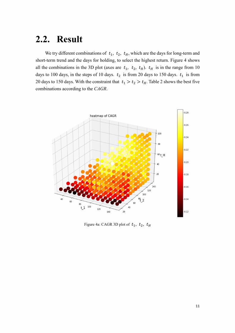
2.2. Result

We try different combinations of ��, ��, �), which are the days for long-term and

short-term trend and the days for holding, to select the highest return. Figure 4 shows

all the combinations in the 3D plot (axes are ��, ��, �)). �) is in the range from 10

days to 100 days, in the steps of 10 days. �� is from 20 days to 150 days. �� is from

20 days to 150 days. With the constraint that �� > �� > �). Table 2 shows the best five

combinations according to the CAGR.

Figure 4a: CAGR 3D plot of ��, ��, �)

12

Figure 4b: CAGR 2D plot of ��, ��

Figure 4c: CAGR 2D plot of ��, �)

13

Figure 4d: CAGR 2D plot of ��, �)

Table 2: Best five combinations based on CAGR

(The best result of each column is bolded)

Z[ Z\ Z] CAGR MDD Sharpe Ratio

1 100.0 90.0 50.0 0.285020 -0.419225 19.122591

2 100.0 90.0 80.0 0.275732 -0.452795 18.105107

3 110.0 100.0 80.0 0.269722 -0.462103 17.258386

4 120.0 100.0 70.0 0.269038 -0.422275 18.200563

5 90.0 80.0 50.0 0.267857 -0.393082 18.567482

To avoid overfitting, we set the threshold to be the highest 5% combinations of

CAGR, which is around 26%, in this study. We keep the combinations which the CAGR

is greater or equals to 26%. Then, we calculate the average ��, ��, �) of this subset

of data, as follow

��̂ = ∑ ��_8̀a , ��̂ = ∑ ��_8̀a , �)bbb = ∑ �)_8̀a ,

where * = g(��, ��, �)), �ABC(��, ��, �)) > 26%}.

14

The results are ��̂ ≈ 111 (2.l�), ��̂ ≈ 91(2.l�), �)bbb ≈ 76 (2.l�) in this study.

The performance is shown in figure 5.

Figure 5: The equity curve of the strategy from 2005 to 2015. Black curve indicates the equity of HSI,

for comparison. Green curve indicates the equity of our strategy. Red curve indicates the drawdown of

our strategy. The bar below are the annual returns of our strategy.

From the above equity curve, we can see that our strategy (green line) had a better

performance comparing to the HSI (black line). Because the CAGR of our strategy is

around 25.41%, while HIS’s CAGR is only 5.7%. But we can also see that the

drawdown of our strategy is also very high, with the maximum value 43.37%, in the

financial crisis period, from the end of 2007.Besides, from 2011 to 2012, our strategy

is also losing money. In order to reduce the loss, some additional constraints are

introduced to help.

15

3. Additional constraints

3.1. SMA of the HSI

We first calculate the n days Simple Moving Average is calculated by the equation:

SMA(-) = �r�Gs�r�G�Fs⋯s�r�Fu ,

$3�u is the price at n days ago. The constraint requires today’s HSI to be greater

that its simple moving average. In this study, we set the n to be ��, which is day for

determining the short-term trend mentioned above. In other words, v0l *�,-.+ =/ ��0�, 8(�) > 0 .-2 w*x3 > *HA)`y(91) 5.+��, ��ℎ������ .

The result of the training period is shown in figure 6. After introducing this

constraint, the CAGR decreases a lot, from 25.41% to 14.92%. However, we can see

that this constraint can effectively stop loss during the period of financial crisis (from

around June 2008). Overall, the maximum drawdown decreases from 43.37% to

37.92%.

Figure 6: The equity curve of adding the constraint “SMA of the HSI”, from 2005 to 2015

16

3.2. SMA of individual stock

The rule is similar to the above constraint, but we are now only considering each

individual stock. In other words, the buy signal would be v0l *�,-.+ =/ ��0�, 8(�) > 0 .-2 $8,3 > *HA�_(91) 5.+��, ��ℎ������ .

$8,3 is the price of an individual stock at time t. *HA�_(-) is the n days simple

moving average of that individual stock. The result is shown in figure 7. This constraint

also helps to reduce the loss, maximum drawdown decreases from 43.37% to 40.18%,

while it can keep the high CAGR which is around 23.92%. It is better than the SMA of

HSI constraint.

Figure 7: The equity curve of adding the constraint “SMA of the individual stock”, from 2005 to

2015

17

3.3. Z-score of individual stock

The z-score will be used to measure the uncertainty. The n days moving standard

deviation of each individual stock will be first calculated by:

σ{(-) = |∑|$8 − $~̂|�-

$~̂ is the average price from time t-n to t. The z-score is calculated by:

�8(-) = $8,3 − *HA8(-)Y8(-)

The reason we add the z-score is to diagnosis the real upward trend. When the price

has a larger upward momentum, which means that the price is increasing and would be

higher than the average price of previous period. We believe that this increasing trend

is reflected by the z-score, in this study, we set the threshold to be 2, and the range of

the previous period n to be t�. Therefore, by adding this constraint the buy signal will

be

v0l *�,-.+ = / ��0�, 8(�) > 0 .-2 |�8(91)| > 2 5.+��, ��ℎ������ .

The result is shown in figure 8. From figure 8, we can see that this constraint can

also reduce the loss. The equity curve does not decrease a lot in the financial crisis

period (from 2008). And the CAGR also does not decrease a lot, only from 25.41% to

22.55%.

18

Figure 8: The equity curve of adding the constraint “Z-score” , from 2005 to 2015

19

3.4. MACD of HSI

There are two simple moving averages used to calculate the MACD. First, the

difference value between them is calculated by: Ix5)`y(-�, -�) = *HA)`y(-�) − *HA)`y(-�)

Then, the MACD is calculated by take the moving average of DIF: HA�I)`y(-�) = *HA�y����(-�)

In this study, we set -� = 12, -� = 26, n� = 9. It means that the buy signal in

this study is determined by v0l *�,-.+= / ��0�, 8(�) > 0 .-2 Ix5)`y(12, 26) 1 HA�I)`y(9)5.+��, ��ℎ������ .

The result is shown in figure 9. It also deceases the drawdown, from 43.37% to

38.19%, while the CAGR also decrease from 25.41% to 24.7%.

Figure 9: The equity curve of adding the constraint “MACD of HSI” , from 2005 to 2015

20

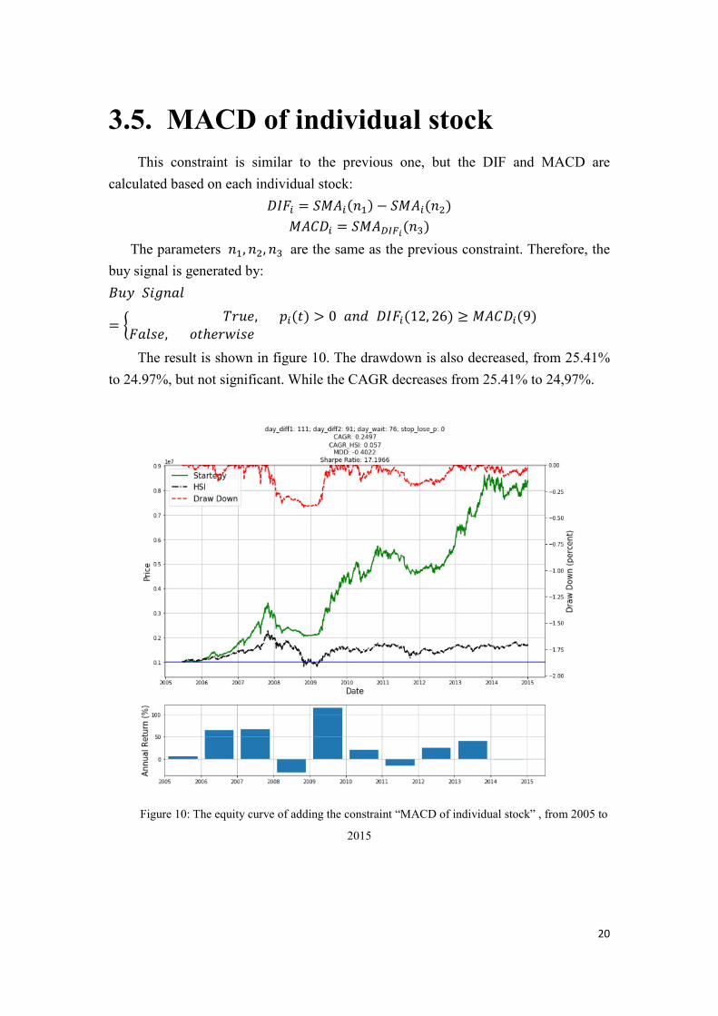
3.5. MACD of individual stock

This constraint is similar to the previous one, but the DIF and MACD are

calculated based on each individual stock: Ix58 = *HA8(-�) − *HA8(-�) HA�I8 = *HA�y�_(-�)

The parameters -�, -�, -� are the same as the previous constraint. Therefore, the

buy signal is generated by: v0l *�,-.+= / ��0�, 8(�) > 0 .-2 Ix58(12, 26) 1 HA�I8(9)5.+��, ��ℎ������

The result is shown in figure 10. The drawdown is also decreased, from 25.41%

to 24.97%, but not significant. While the CAGR decreases from 25.41% to 24,97%.

Figure 10: The equity curve of adding the constraint “MACD of individual stock” , from 2005 to

2015

21

3.6. Comparison

Table 3: Performance of the strategies, from 2005 to 2015

(The best result of each row is bolded)

Original SMA of

HSI

SMA of

stock

Z-score MACD of

HSI

MACD of

stock

CAGR

(%)

25.41 14.92 23.92 22.55 24.70 24.97

MDD (%) -43.37 -37.92 -40.18 -27.96 -38.19 -40.22

Sharpe

Ratio

16.68 9.36 17.15 17.72 17.37 17.20

Table 3 shows the comparison of all methods which are used in this study. The

best result of each row is bolded. We can see that all constraints can help decrease the

drawdown. Since maximum drawdowns of all constraints are less than the original

strategy. The “Z-score” constraint has the best performance in reducing the drawdown,

which decrease the MDD from -43.37% to -27.96%. It also has the best performance in

term of Sharpe ratio, which means it earns more than others under the same amount of

risk for CAGR, the original strategy has the highest CAGR, which is 25.41%. The

second high is MACD of stock, with 24.97%. Overall, ‘Z-score” performs better in the

training.

22

4. Testing

Historical data from 1/1/2015 to 1/1/2018 is used to test the strategy. The process

is similar to the training:

1. Select the stocks by using the criterions mentioned in section 1.1.

2. Trading according to section 1.3.

3. Trading with constraints according to section 3.1. – 3.5.

4.1. Testing results

23

4.1.1. Original

Original result is shown in figure 11. The equity curve of our strategy is closed to

the equity of HSI, except the period during 11/2015 to 07/2016. Our strategy loss less

than HSI index. CAGR is closed to the HSI’s CAGR, which are 8.17% and 8.07%

respectively.

Figure 11: The original equity curve from 2015 to 2018

24

4.1.2. SMA of HSI

Figure 12 shows the result of the SMA of HSI constraint. The CAGR of this

constraint is larger than the original one, which is 9.13%. And the MDD is also less,

which is 25.47%. Besides, we can also see that the constraint did well to stop the

drawdown in the period from 11/2015 to 07/2016. Since our equity curve fluctuate

around the blue line (original capital), which means that our strategy is stopped to loss

during this period, while HSI’s equity curve drops below the blue line.

Figure 12: The equity curve of adding the constraint “SMA of the HSI” , from 2015 to 2018

25

4.1.3. SMA of stock

Figure 13 shows that the SMA of stock constraint performed similar to the original

strategy, the equity curve is also closed to the HSI curve. But the CAGR is only 7.65%,

slightly less than the CAGR of HSI.

Figure 13: The equity curve of adding the constraint “SMA of the individual stock” , from 2015

to 2018

26

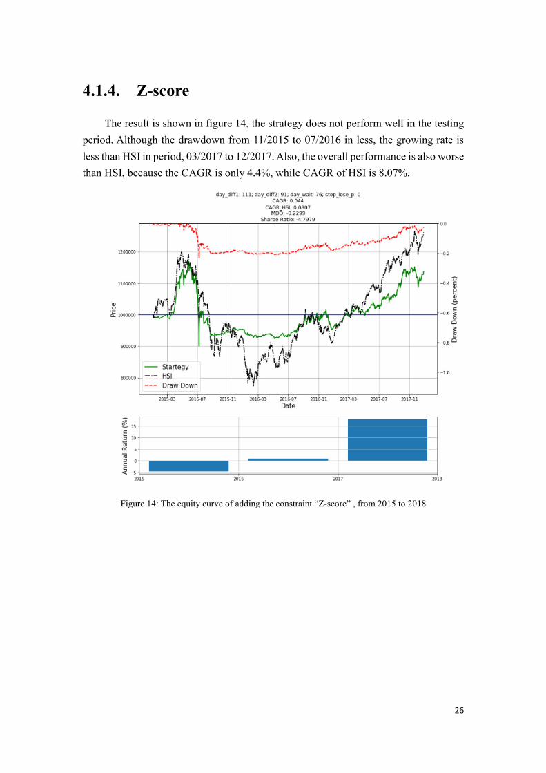
4.1.4. Z-score

The result is shown in figure 14, the strategy does not perform well in the testing

period. Although the drawdown from 11/2015 to 07/2016 in less, the growing rate is

less than HSI in period, 03/2017 to 12/2017. Also, the overall performance is also worse

than HSI, because the CAGR is only 4.4%, while CAGR of HSI is 8.07%.

Figure 14: The equity curve of adding the constraint “Z-score” , from 2015 to 2018

27

4.1.5. MACD of HSI

We can see from figure15, this strategy also performed normally. The curve is similar

to the HSI, and also the origianal strategy. The CAGR of this strategy is only 7.63%

which is less than the HSI’s CAGR.

Figure 15: The equity curve of adding the constraint “MACD of the HSI” , from 2015 to 2018

28

4.1.6. MACD of stock

The result is shown in figure 16. We can see that this strategy can reduce the drawdwon,

and also has a better performance in the year 2017, comparing to the other strateries.

Its CAGR is 9.26%, which is the highest among all strategy mentioned above.

Figure 16: The equity curve of adding the constraint “MACD of individual stock” , from 2015 to

2018

29

4.2. Comparison

Table 4: Performance of the strategies, from 2015 to 2018

(The best result of each row is bolded)

Original SMA of

HSI

SMA of

stock

Z-score MACD of

HSI

MACD of

stock

CAGR

(%)

8.17 9.13 7.65 4.4 7.63 9.26

MDD (%) -28.05 -25.47 -25.75 -22.99 -25.76 -25.62

Sharpe

Ratio

0.11 1.14 -0.47 -4.80 -0.49 1.26

Table 4 shows the performance of all methods in the testing period. We can see

that the “MACD of stock” has the highest CAGR and Sharpe Ratio. But all methods do

not perform well in the testing. Since the CAGRs are small, comparing with the HIS,

some of them are even lower that the HIS’s CAGR, while others are just slightly better

than HIS’s CAGR. Also, the drawdowns of all methods are high, they range from 22%

to 28%, while the CAGRs are only around 7% to 9% in general. It means that these

strategies lose more while earn less. We can also see it from the Sharpe ratio, the

positive Sharpe ratios are only in the range from 0.11 to 1.26, which means that the

additional profits earned under risk are low. Even some of the strategies have negative

Sharpe ratios. In other words, they are losing money under the risk.

30

5. Conclusion

Although our strategies have high CAGRs in the training, they do not perform well

in the testing. There are some possibilities:

1. Our strategies do not perform well when the market is going down:

Even in the training set, the equity curves of our strategies are also going

downward, when the market is going down. The reason why we still have an

overall good result in the training is because in 10 years scale, the market is

generally going up. Therefore, our strategies can earn back the money. In the

testing, the market is dropping 1/3 of the time. Which may yield our strategies

have negative return during that period.

2. The ratio of training and testing size are not suitable in stock market:

We used around 75% training and 25% testing, which is 10 years for training and

3 years are testing. But the market may be changing. In other words, when we

are training the strategies using the past data, the strategies can really capture the

properties of the market. So, they can have a positive return. But, the

characteristics of the market is changing. Therefore, the strategies will not have

the same performance under a market with changed features. One possibility is

that trend is significant in the longer scale (e.g. “Days” or “Week”) in the past.

So, our strategies can capture the trend in longer scale. But, nowadays, as

technology becoming more popular. The trading frequency is much higher than

before, which means that the trend becomes shorter (e.g. “Minutes”, “Seconds”).

Since our strategies are trained with past data. The trained strategies may not

work in nowadays.

3. We may overfit/underfit:

We used the step of 10 days to try the best combinations of the parameters. But,

the best cluster of the combinations may be form in between each 10 days, or

maybe the best combinations are beyond the range that we are testing. Besides,

the best combinations do not ensure that it is also the best combinations in the

testing.

31

6. Discussion

There are some ideas to improve the strategy:

1. Include “Short selling”:

In this report, we are only buying the stocks. In other words, the only way that

our strategy can earn money is when the market is going up. Therefore, by

adding the short selling signal, we wish to have more opportunity. And this

may also improve the situation of losing money when the market is going down.

2. Include “Stop earn” and “Stop loss”:

We did not consider the stopping signal in the report. It may decrease the profit

of our strategy, since we may miss the best exit opportunity. For example, the

ideal case would be buying the stock at the lowest price, selling it in the peak.

But our strategy does not consider the exit position, which means that we may

selling the stock when it passed the peak and is going downward. It will reduce

the profit. Therefore, by adding the stop signals, both “Stop earn” and “Stop

loss” may help to maximum our profit.

3. Focus more on the recent data while training:

As we mentioned above, the outdated data may affect our strategy in the way

that the features of the training set are different from the testing set. Therefore,

the trained strategy may perform badly in the testing. So, if we focus more on

the recent data, then the training and testing set will have similar features. The

strategy may have a similar performance as the training.

4. Adding more constraints:

In this study, we just added one constraint to the original strategy. It may not

be enough to increase the accuracy of diagnosing the right signals (either buy

or sell). Therefore, we can combine more than one constraint to the original

strategy, to increase the chance of capturing the right signals. We may also test

the best combinations of the constraint in the future.