Modular meta-learning

Ferran Alet, Tomas Lozano-Perez, Leslie P. KaelblingMIT Computer Science and Artificial Intelligence Laboratory

{alet,tlp,lpk}@mit.edu

Abstract: Many prediction problems, such as those that arise in the context ofrobotics, have a simplifying underlying structure that, if known, could acceleratelearning. In this paper, we present a strategy for learning a set of neural networkmodules that can be combined in different ways. We train different modular struc-tures on a set of related tasks and generalize to new tasks by composing the learnedmodules in new ways. By reusing modules to generalize we achieve combinato-rial generalization, akin to the ”infinite use of finite means” displayed in language.Finally, we show this improves performance in two robotics-related problems.

1 Introduction

In many situations, such as robot learning, training experience is very expensive. One strategy forreducing the amount of training data needed for a new task is to learn some form of prior or biasusing data from several related tasks. The objective of this process is to extract information that willsubstantially reduce the training-data requirements for a new task. This problem is a form of transferlearning, sometimes also called meta-learning or “learning to learn” [1, 2].

Previous approaches to meta-learning have focused on finding distributions over [3] or initial valuesof [4, 5] parameters, based on a set of “training tasks,” that will enable a new “test task” to belearned with many fewer training examples. Our objective is similar, but rather than focusing ontransferring information about parameter values, we focus on finding a set of reusable modules thatcan form components of a solution to a new task, possibly with a small amount of tuning. Byreusing our learned modules, we aim at combinatorial generalization[6, 7, 8]; this is akin to thereuse of words to construct many possible sentences. We propose that this ”infinite use of finitemeans” (Von Humboldt) can be a scalable approach towards transfer and generalization.

Modular approaches to learning have been very successful in structured tasks such as natural-language sentence interpretation [9], in which the input signal gives relatively direct informationabout a good structural decomposition of the problem. We wish to address problems that may ben-efit from a modular decomposition but do not provide any task-level input from which the structureof a solution may be derived. Nonetheless, we adopt a similar modular structure and parameter-adaptation method for learning reusable modules, but use a general-purpose simulated-annealingsearch strategy to find an appropriate structural decomposition for each new task.

We provide an algorithm, called BOUNCEGRAD, which learns a set of modules and then combinesthem appropriately for a new task. We demonstrate its effectiveness by comparing it to MAML [4],a popular meta-learning method, on a set of regression tasks that represent the types of prediction-learning problems that are faced by robotics systems, and show that we achieve better predictionperformance from a few training examples, and can be much faster to train. In addition, we showthat this modular approach offers a strategy for explaining learned solutions to new tasks: by ob-serving the modules that are used in a new task, we can relate this task to previous tasks that use thesame modules. This approach also offers opportunities for verification and validation: the modulesdiscovered during meta-learning may be subjected to computationally expensive analytical or em-pirical validation techniques off-line; they can then be recombined to address new tasks, generatingsolutions that can be validated more efficiently as compositions of previously understood modules.

2 Related Work

Our work draws primarily from two sources: multi-task meta-learning and modular networks.Prominent examples of meta-learning in robotic domains are MAML [4] and follow-up work [5, 10].They perform “meta-training” on a set of related tasks with the goal of finding network weightsthat serve as a good starting point for a few steps of gradient descent in each task. Others

2nd Conference on Robot Learning (CoRL 2018), Zurich, Switzerland.

Figure 1: All methods train on a set of related tasks and obtain some flexible intermediate repre-sentation. Parametric strategies such as MAML (left) learn a representation that can be quicklyadjusted to solve a new task. Our modular meta-learning method (middle) learns a repertoire ofmodules that can be quickly recombined to solve a new task. A combination of MAML and mod-ular meta-learning (right) learn initial weights for modules that can be combined and adapted for anew task.

[11, 12, 13, 14, 15] perform different types of parametric changes in the network’s computationconditioned on few examples. We adapt the same basic setting, but rather than finding good startingweights, we find a good set of modules for later structural combination; see figure 1. This is akin tothe distinction in AI and cognitive science between parameter change vs. structural change [16, 17].

Neural module networks [9] provide an elegant mechanism for training a set of individual modulesthat can be recombined to solve new problems, when the input has enough signal to guess an appro-priate modular decomposition. Johnson et al. [18] later showed that the structure controller could betrained with RL; others applied similar frameworks to get more interpretability [19] or to generalizeacross robotic tasks with neural programs[20]. However, as far as we know, this framework has notbeen applied in problems where the input does not give enough information about an appropriatestructure.

Structured networks have been used for meta-learning in the reinforcement-learning setting. Devinet al. [21] use a fixed composition of two functions, one related to the robot and one to the task.Frans et al. [22] jointly optimize a master policy and a set of sub-policies (options) that can be usedto solve new problems; this method can be seen as having a single fixed scheme of combination viathe master policy; it is in contrast to our ability to handle a variety of computational compositions.PATHNET [23] is closely related to our work. The architecture is layered, with several modulesin each layer. An evolutionary algorithm determines gates on the connections among the modules.After training on an initial task, the weights in the modules that contribute to the solution to that taskare frozen, and then the architecture is trained on a second task. If the tasks are sufficiently related,the modules learned in the first task can be directly re-used to make learning more efficient in thesecond task. Meyerson and Miikkulainen [24] and later Liang et al. [25] expanded these ideas tothe multitask setting with two particular compositional schemes: soft layer ordering and routing inDAGs. We propose a general framework of which these are two important sub-cases. Moreover, weoperate in the meta-learning setting where, with few points per task, it is very easy to prematurelyoptimize the structure and run into local optima, as shown in figure 5. Therefore, we believe usingsimulated annealing rather than gradient descent[24] or irreversible evolution[25] may be a better fitfor our setting.

3 Modular meta-learning

We explore the problem of modular meta-learning in the context of supervised learning problems,in which training and validation sets of input-output pairs are available. Such problems arise inrobotics, particularly in learning to predict a next state based on information about previous statesand actions. We believe that techniques similar to ours can be applied to reinforcement-learningproblems as well, but do not explore that in this paper. We use the same meta-learning problemformulation as Finn et al.[4] used to apply MAML to supervised learning problems. We assumean underlying distribution p(T ) over tasks: a task is a joint distribution PT (x, y) over (x, y) pairs.

2

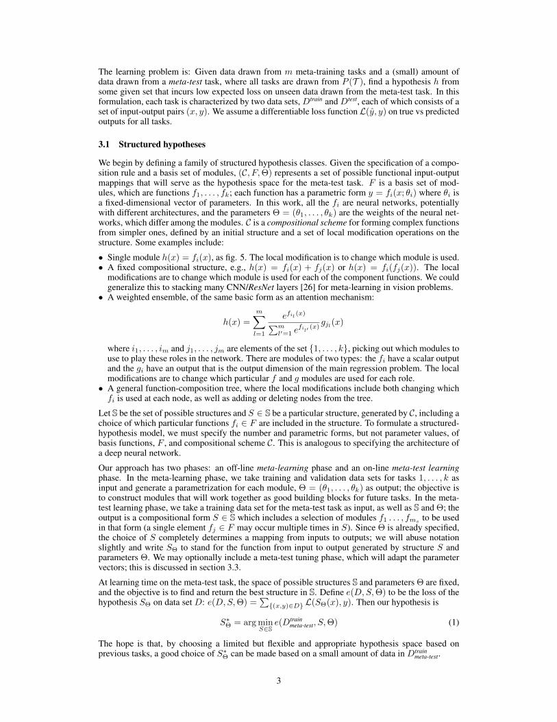
The learning problem is: Given data drawn from m meta-training tasks and a (small) amount ofdata drawn from a meta-test task, where all tasks are drawn from P (T ), find a hypothesis h fromsome given set that incurs low expected loss on unseen data drawn from the meta-test task. In thisformulation, each task is characterized by two data sets, Dtrain and Dtest, each of which consists of aset of input-output pairs (x, y). We assume a differentiable loss function L(y, y) on true vs predictedoutputs for all tasks.

3.1 Structured hypotheses

We begin by defining a family of structured hypothesis classes. Given the specification of a compo-sition rule and a basis set of modules, (C, F,Θ) represents a set of possible functional input-outputmappings that will serve as the hypothesis space for the meta-test task. F is a basis set of mod-ules, which are functions f1, . . . , fk; each function has a parametric form y = fi(x; θi) where θi isa fixed-dimensional vector of parameters. In this work, all the fi are neural networks, potentiallywith different architectures, and the parameters Θ = (θ1, . . . , θk) are the weights of the neural net-works, which differ among the modules. C is a compositional scheme for forming complex functionsfrom simpler ones, defined by an initial structure and a set of local modification operations on thestructure. Some examples include:

• Single module h(x) = fi(x), as fig. 5. The local modification is to change which module is used.• A fixed compositional structure, e.g., h(x) = fi(x) + fj(x) or h(x) = fi(fj(x)). The local

modifications are to change which module is used for each of the component functions. We couldgeneralize this to stacking many CNN/ResNet layers [26] for meta-learning in vision problems.

• A weighted ensemble, of the same basic form as an attention mechanism:

h(x) =

m∑l=1

efil (x)∑ml′=1 e

fil′

(x)gjl(x)

where i1, . . . , im and j1, . . . , jm are elements of the set {1, . . . , k}, picking out which modules touse to play these roles in the network. There are modules of two types: the fi have a scalar outputand the gi have an output that is the output dimension of the main regression problem. The localmodifications are to change which particular f and g modules are used for each role.

• A general function-composition tree, where the local modifications include both changing whichfi is used at each node, as well as adding or deleting nodes from the tree.

Let S be the set of possible structures and S ∈ S be a particular structure, generated by C, including achoice of which particular functions fi ∈ F are included in the structure. To formulate a structured-hypothesis model, we must specify the number and parametric forms, but not parameter values, ofbasis functions, F , and compositional scheme C. This is analogous to specifying the architecture ofa deep neural network.

Our approach has two phases: an off-line meta-learning phase and an on-line meta-test learningphase. In the meta-learning phase, we take training and validation data sets for tasks 1, . . . , k asinput and generate a parametrization for each module, Θ = (θ1, . . . , θk) as output; the objective isto construct modules that will work together as good building blocks for future tasks. In the meta-test learning phase, we take a training data set for the meta-test task as input, as well as S and Θ; theoutput is a compositional form S ∈ S which includes a selection of modules f1 . . . , fms

to be usedin that form (a single element fj ∈ F may occur multiple times in S). Since Θ is already specified,the choice of S completely determines a mapping from inputs to outputs; we will abuse notationslightly and write SΘ to stand for the function from input to output generated by structure S andparameters Θ. We may optionally include a meta-test tuning phase, which will adapt the parametervectors; this is discussed in section 3.3.

At learning time on the meta-test task, the space of possible structures S and parameters Θ are fixed,and the objective is to find and return the best structure in S. Define e(D,S,Θ) to be the loss of thehypothesis SΘ on data set D: e(D,S,Θ) =

∑{(x,y)∈D} L(SΘ(x), y). Then our hypothesis is

S∗Θ = arg minS∈S

e(Dtrainmeta-test, S,Θ) (1)

The hope is that, by choosing a limited but flexible and appropriate hypothesis space based onprevious tasks, a good choice of S∗Θ can be made based on a small amount of data in Dtrain

meta-test.

3

At meta-learning time, S is specified, and the objective is to find parameter values Θ that constitutea set of modules that can be recombined to effectively solve each of the training tasks. We usevalidation sets for the meta-training tasks to avoid choosing Θ in a way that over-fits. Our trainingobjective is to find Θ that minimizes the average generalization performance of the hypotheseschosen by equation 1 using parameter set Θ:

J(Θ) =

m∑j=1

e(Dtestj , arg min

S∈Se(Dtrain

j , S,Θ),Θ) . (2)

3.2 Learning algorithm

The optimization problems specified by equations 1 and 2 are in general quite difficult, requiring amixed continuous-discrete search in a space with many local optima. In this section, we describethe BOUNCEGRAD algorithm, which performs local searches based on a combination of simulatedannealing and gradient descent to find approximately optimal solutions to these problems.

3.2.1 Meta-test learning phase

In the meta-test learning phase, we have fixed the parameters Θ and only need to find an optimalstructure S ∈ S according to the objective in equation 1. We use simulated annealing [27] toperform this search: it is a local search strategy that uses stochasticity to avoid local optima andhas asymptotic optimality guarantees. We start with an initial structure, then randomly proposestructural changes using local modification operators associated with the compositional scheme S,accept the change if it decreases the error on the task and, with some probability, even if it does not.

procedure ONLINE(Dtrainmeta−test , S, Θ, T0, ∆T , Tend )

S = random simple structure from Sfor T = T0; T = T −∆T ; T < Tend do

S′ = PROPOSES(S)if ACCEPT(e(D,S′,Θ), e(D,S,Θ), T ) then S = S′

return Sprocedure ACCEPT(v′, v, T )

return v′ < v or rand(0, 1) < exp{(v − v′)/T}

In order for simulated annealing to converge, the temperature parameter T must be decreased overtime. The schedule we use decreases too quickly to satisfy theoretical convergence guarantees, yet ispractically effective. Given the training set for the meta-test task, we run ONLINE(Dtrain

meta−test ,S,Θ)to obtain a hypothesis for that task.

3.2.2 Meta-learning phase

To perform the optimization in equation 2, we might use an algorithm that, in the outer loop, per-forms optimization over continuous parameters Θ, where the evaluation of Θ consists of runningprocedure ONLINE on each of the training data sets, and evaluating the resulting structural hypothe-ses using the validation sets. This strategy is ineffective because of the prevalence of bad localoptima in the space, as illustrated in figure 5. As in clustering, we can smooth out some local optimaby changing the objective function, although we will do so only during search, so our meta-testobjective will remain the same. We formulate a smoothed objective

J(Θ, T ) =

m∑j=1

ES∼MC(S,v(s;Θ),T )e(Dtestj , S,Θ) (3)

Here, MC(S, v, T ) is the Markov chain induced by executing the simulated-annealing sampler inthe structure space S using its proposal operator, with score function v(s; Θ) = e(Dtrain

j , s,Θ) andfixed temperature T . Rather than trying to find the Θ values that work best when we choose the beststructure S, we will instead try to find Θ values that work best in expectation given the distribution ofstructures induced by the Markov chain. This space is smoother and less susceptible to local optima.At the same time as we are optimizing Θ via stochastic gradient, we will cool the temperature of theMarkov chain. As T approaches 0, the objective J becomes the same as our original objective J .

4

(a) (b)

Figure 2: (a) A schematic view of the optimization landscape over Θ and T . At each point, there is adistribution over structures. As temperature decreases, the variance of the distribution decreases andmodules become more specialized. (b) benchmarked robotic domains: MIT push dataset [28](top),action (throwing a ball) in the Berkeley MHAD dataset [29] (bottom).

Given particular structures Sj , then for each task Tj , we know the parametric form of a differentiablefeed-forward function that has parameters drawn from Θ, but possibly with parameter tying withinand across the tasks due to re-use of the basis functions in F and possibly with some parameters inΘ left unused. We can adjust Θ using stochastic gradient descent, as defined in procedure GRAD.It takes the structures and training data as input, as well as a step size η and performs one step ofstandard stochastic gradient descent, or any alternative optimizer:

procedure GRAD(Θ, S1, . . . , Sm, Dtest1 , . . . , Dtest

m , η)∆ = 0for j = 1 . . .m do

(x, y) = rand elt(Dtestj ); ∆ = ∆ +∇ΘL(SjΘ(x), y)

Θ = Θ− η∆

However, we do not know the appropriate structure for each task, and so, according to the smoothedcriterion in equation 3, we sample structures using a stochastic process based on simulated anneal-ing. We define a procedure BOUNCE that takes a simulated annealing step on a structural hypothesisfor each task, using the current Θ values, for a fixed temperature T :

procedure BOUNCE(S1, . . . , Sm, Dtrain1 , . . . , Dtrain

m ,T , S, Θ)for j = 1 . . .m do

S′j = ProposeS(Sj ,Θ)

if Accept(e(Dtrainj , S′j ,Θ), e(Dtrain

j , Sj ,Θ), T ) then Sj = S′j

Finally, we combine these methods into an overall algorithm for optimizing equation 1 via optimiz-ing equation 3 and decaying T :

procedure BOUNCEGRAD(S, Dtrain1 , . . . , Dtrain

m , Dtest1 , . . . , Dtest

m , η, T0,∆T , Tend )S1, . . . , Sm = random simple structures from S; Θ = neural-network weight initializationfor T = T0; T = T −∆T ; T < Tend do

BOUNCE(S1, . . . , Sm, Dtrain1 , . . . , Dtrain

m , T , S, Θ)GRAD(Θ, S1, . . . , Sm, Dtest

1 , . . . , Dtestm , η)

We can think of the state of the optimization algorithm as consisting of both the parameters Θ andthe temperature T ; these values induce a distribution on structures. The optimization landscapeis illustrated in figure 2a. At high temperatures, the distribution over structures is diffuse and themodules will tend to be very generalized. As the temperature decreases, modules can specialize toperform well at the roles they are being selected to play in the structures.

3.3 Parameter tuning in online phase

In the basic ONLINE method, we search for the best structure for the new task, without modifyingparameters Θ. In fact, in many cases it may be useful to perform some additional parameter opti-

5

mization as well. One strategy would be to proceed as we have described before, running BOUNCE-GRAD on the training tasks to get Θ, finding the best S for the meta-test task using ONLINE, andthen taking some gradient steps on Θ, given S, to better optimize loss onDtrain. However, we can dobetter by incorporating the objective of MAML more deeply into both ONLINE and BOUNCEGRAD,by redefining the inner error function used in the optimization criterion for Θ: instead of using Θdirectly, we will evaluate the result of taking one (or a few) gradient steps away from Θ, specializedto optimize D. So, eMAML(D,S,Θ) =

∑{(x,y)∈D} L(SO(Θ,D,S)(x), y), where the optimized pa-

rameters O(Θ, D, S) are obtained by a gradient update: O(Θ, D, S) = Θ− η∇Θe(D,S,Θ). Then,the meta-learning objective becomes

JMAML(Θ) =

m∑j=1

e(Dtestj , arg min

S∈SeMAML(Dtrain

j , S,Θ),Θ) (4)

We can therefore use eMAML in place of e in the GRAD and ONLINE procedures, and perform a fewadditional gradient steps on Θ after obtaining the structure from ONLINE. We will call this overallalgorithm MOMA, MOdular MAml.

4 Experiments

We compare four different learning approaches: training a single network using the combined datafrom all tasks (POOLED), training a single network using the MAML criterion, training a modularnetwork without weight adaptation in the online training (BOUNCEGRAD), and training a modu-lar network with MAML adaptation in the online training (MOMA). To make the comparisonsas fair as possible, for experiments on a given data set, all networks have the same shape: gen-erally, a feedforward structure of 3–4 layers. We selected a set of layer sizes so that POOLEDand MAML had about 10 times as many parameters as the structured methods, to compensate forBOUNCEGRAD and MOMA having about 10 modules to combine. We also verified that none ofthe algorithms’ performance was sensitive to modest changes in these parameters. We used Py-Torch and ADAM[30, 31]; the MAML code was adapted from Rakelly [32]. The code is available onhttps://github.com/FerranAlet/modular-metalearning. The target output values y in alldata-sets were standardized to have mean 0 and standard deviation 1. The loss function then assignsloss 100 to a mean squared error of 1. More experimental details are available in the supplement.

We tested these methods in three domains: simple functional relationships, predicting the result ofa robot manipulator pushing an object, and predicting the next frame of a kinematic skeleton basedon previous frames using motion-capture data. The last two domains represent the main motivationfor this work: a robot’s experience of interacting with various entities in real-world situations shouldenable it to learn more efficiently about a new entity in a new situation. There is typically some sen-sible decomposition of the prediction function, but that decomposition is not known in advance. Wehope that BOUNCEGRAD can find an appropriate decomposition and that doing so will significantlyleverage learning, as well as reveal interesting structure, in the new domain.

An additional advantage of BOUNCEGRAD is computational efficiency. Unlike MAML, it does nothave extra gradient steps embedded in the inner loop at meta-training time, which offers some effi-ciency; in addition, forward and backward passes can be done much more efficiently on GPUs byparallelizing over tasks. MAML is generally faster at online training time, since BOUNCEGRAD hasto search over structures. However, this training took at most 10 seconds in our examples. More-over, to store a structure we only need a few integers, compared to storing a whole set of weights forparametric methods.

4.1 Functions

We begin by testing on an extended version of the sine-function prediction problem [4], whichconsisted of data-sets generated from functions of the form sin(ax + b) for varying values of aand b. The compositional scheme for BOUNCEGRAD is h(x) = fi(fj(x)); F consists of 20 feed-forward neural networks, 10 with 1 hidden layer and 10 with 2. In our experiments in this sectionMAML and POOLED use the same architecture as the original MAML experiments. We constructan additional illustrative domain consisting of sums of pairs of common non-linear functions, suchas exp and abs, scaled so the output is contained in the range [−1,+1], generating 162 possible

6

Figure 3: Random functions (left); BOUNCEGRAD (center) and MOMA (right) modules. All butone BOUNCEGRAD modules(blue) are nearly identical to a basis function(red).

Dataset POOLED MAML BOUNCEGRAD MOMA Structure

Parametrized sines 98.1 26.5 32.5 19.8 composition

Sum of functions (1-4pts) 32.7 19.7 12.8 18.0 sum

Sum of functions (16pts) 31.9 8.0 0.4 0.4 sum

MIT push: known objects 21.5 18.5 16.7 14.9 attention

MIT push: new objects 18.4 16.9 17.1 17.0 attention

Berkeley MoCap: known actions 35.7 35.5 32.2 31.9 concatenate

Berkeley MoCap: new actions 79.5 77.7 77.0 73.8 concatenateTable 1: Summary of results; lower is better; bold results are not significantly different from best.

prediction tasks. We use 230 randomly selected tasks for meta-training and a different task fortesting. Example functions are shown on the left of figure 3. We use the same architectures for thisdomain as for the sine domain, except that the compositional scheme is h(x) = fi(x) + fj(x).

The results are shown in table 2. As expected, training a single network on pooled data from allthe tasks (POOLED) works poorly in all of these domains. In the sine domain, MAML outperformsBOUNCEGRAD because the detailed parameter values are critical to performing well in a new do-main, but MOMA significantly improves on both methods, showing that both the structure andgradient meta-learning methods are useful. For sums of functions, we report results in two cases:one in which we average over performance for 1–4 training examples, and one for 16 training ex-amples. With a small amount of online training data, BOUNCEGRAD outperforms other methodsbecause it has the proper structural prior. With more data, all methods improve, but BOUNCEGRADand MOMA improve on MAML. The plots in the middle and right of figure 3 show some of the basismodules learned by BOUNCEGRAD and MOMA, respectively. Those learned by BOUNCEGRADare an almost perfect recovery of the actual primitives used to generate the data, even though thealgorithm had no information about those functions; MOMA has found similar functional shapes,yet with different values because it can still modify its parameters at online training time.

4.2 Learning to model results of pushing actions

An important sub-problem in robot manipulation is to acquire models of the effects of the robot’smotor actions on the objects in the world. The MIT push data-set [28] contains the results of exe-cuting pushing actions with a manipulator hand, for 11 different objects with different shapes on 4surfaces with different friction properties. The behavior of the object on these surfaces is close toquasi-static , so the state can be characterized by an input x consisting of: position of the object (2d),orientation of the object (1d), position of the pusher (2d), and velocity of the pusher (2d). Given this7-d input, the objective is to predict the 3-d change in the object’s position and orientation. Eachtask represents experience with a particular object on a particular surface.

The compositional scheme for BOUNCEGRAD is the weighted ensemble described in section 3.1;F consists of 20 feedforward neural networks, 10 attention modules and 10 regressors. We considertwo different meta-learning scenarios. In the first, the object-surface combination in the test case was

7

Figure 4: Shared modules show internal structure of the datasets (left–pushing; right–motion). Inparticular, less important factors (surfaces and subjects) do not change the structure while biggerchanges (objects and actions) do. Within the structural changes, there is more sharing betweenconceptually similar datasets.

present in some meta-training task; in the second, the objects used in the meta-training tasks differfrom the object used in the test task. The results in table 2 show that, for previously encounteredobjects, MOMA performs best, and BOUNCEGRAD outperforms MAML. For unknown objects, allthree approaches perform roughly equivalently.

Another important aspect of the structured hypothesis space is that it can give us insight into therelationships between tasks. Figure 4 illustrates the structural relationships that were uncovered inthis data. The matrix on the left is indexed according to which object was being pushed. The entry inlocation i, j represents the average percentage of modules shared by the structure learned to predictresults for object i and the structure learned for object j. We can see it distinguishes 3 clusters ofdata: butterfly, all ellipses, and all triangles. The biggest rectangle shares modules with the biggesttriangle, probably due to similar size and aspect ratio. The matrix labeled ”Surfaces” does not showdependence on the surface, as expected for the quasi-static regime.

4.3 Predicting skeleton configurations

Robots that interact with humans should be able to understand and predict human action, both forthe purposes of safety and for task-driven collaboration. We applied meta-learning to this problem,using data from the Berkeley MHAD motion capture dataset [29]. This domain is dynamic, andso we use three previous configurations (at intervals of 0.1 sec) of a human skeleton to predict thenext one. Each configuration is characterized by one 3-d position and 90 joint angles describinga kinematic tree, so the input has dimension 279 and the output has dimension 93. There are 12subjects performing 11 different actions several times, for a few seconds each.

We constructed a compositional scheme for BOUNCEGRAD that is related to this task. It has afixed first layer with 128 output units to compress the input, which is the same for all structures,and independent “parallel” modules that take those 128 inputs and produce kinematic sub-trees foreach body part (2 legs, 2 arms, and torso). For MAML and POOLED we use a single architectureof the same depth with 4 times more parameters. We again consider two different meta-learningscenarios. In the first, the activities used in the training task are the same as the activities used inthe meta-test task, but the human actor varies; in the second, the activities used in the training tasksdiffer from the activity used in the test task. The results in table 2 show that, for known activities,BOUNCEGRAD and MOMA perform best. For unknown activities, none of the methods performvery well, but MOMA outperforms the others. We obtain a similar pattern of correlation amongshared modules, shown in figure 4, in which there is significant module-sharing among similar tasksand no real pattern of module-sharing among human actors.

4.4 Conclusion

We have demonstrated that modular compositional structure can provide a useful basis for transfer-ring learned competence from previous tasks to new tasks. It can also yield insight into the under-lying structure of the domain. We believe this combinatorial generalization is a promising route toscale to large numbers of tasks and continual learning settings as we can increase our knowledgein modular ways without forgetting previously learned concepts. The structural information to beprovided in advance is a few lines of code to describe the possible modifications that can be made toa structure, which is not much more than would be required for specifying a typical neural network.

8

Acknowledgments

We gratefully acknowledge support from NSF grants 1420316, 1523767 and 1723381 and fromAFOSR grant FA9550-17-1-0165. F. Alet is supported by a La Caixa fellowship. Any opinions,findings, and conclusions or recommendations expressed in this material are those of the authorsand do not necessarily reflect the views of our sponsors.We want to thank Zi Wang for her assistance in setting up the experiments, Maria Bauza for her helpwith the MIT push dataset and Rohan Chitnis for his comments on an initial draft. Finally, we thankreviewers for their useful suggestions.

References[1] J. Schmidhuber. Evolutionary principles in self-referential learning, or on learning how to

learn: the meta-meta-... hook. PhD thesis, Technische Universitat Munchen, 1987.

[2] S. Thrun and L. Pratt, editors. Learning to learn. Springer Science & Business Media, 2012.

[3] A. Wilson, A. Fern, S. Ray, and P. Tadepalli. Multi-task reinforcement learning: A hierarchicalBayesian approach. In Proceedings of the 24th International Conference on Machine Learning.ACM, 2007.

[4] C. Finn, P. Abbeel, and S. Levine. Model-agnostic meta-learning for fast adaptation of deepnetworks. In D. Precup and Y. W. Teh, editors, Proceedings of the 34th International Confer-ence on Machine Learning, volume 70 of Proceedings of Machine Learning Research, pages1126–1135, 2017.

[5] A. Nichol, J. Achiam, and J. Schulman. On first-order meta-learning algorithms. CoRR,abs/1803.02999, 2018. URL http://arxiv.org/abs/1803.02999.

[6] W. von Humboldt. On language: On the diversity of human language construction and itsinfluence on the mental development of the human species. 1836/1999.

[7] N. Chomsky. Aspects of the Theory of Syntax, volume 11. MIT press, 1964.

[8] P. W. Battaglia, J. B. Hamrick, V. Bapst, A. Sanchez-Gonzalez, V. Zambaldi, M. Malinowski,A. Tacchetti, D. Raposo, A. Santoro, R. Faulkner, et al. Relational inductive biases, deeplearning, and graph networks. arXiv preprint arXiv:1806.01261, 2018.

[9] J. Andreas, M. Rohrbach, T. Darrell, and D. Klein. Neural module networks. In Proceedingsof the IEEE Conference on Computer Vision and Pattern Recognition, pages 39–48, 2016.

[10] T. Yu, C. Finn, A. Xie, S. Dasari, T. Zhang, P. Abbeel, and S. Levine. One-shot imitationfrom observing humans via domain-adaptive meta-learning. arXiv preprint arXiv:1802.01557,2018.

[11] Y. Duan, M. Andrychowicz, B. Stadie, O. J. Ho, J. Schneider, I. Sutskever, P. Abbeel, andW. Zaremba. One-shot imitation learning. In Advances in neural information processingsystems, pages 1087–1098, 2017.

[12] Y. Duan, J. Schulman, X. Chen, P. L. Bartlett, I. Sutskever, and P. Abbeel. Rl 2: Fast reinforce-ment learning via slow reinforcement learning. arXiv preprint arXiv:1611.02779, 2016.

[13] M. Andrychowicz, M. Denil, S. Gomez, M. W. Hoffman, D. Pfau, T. Schaul, B. Shillingford,and N. De Freitas. Learning to learn by gradient descent by gradient descent. In Advances inNeural Information Processing Systems, pages 3981–3989, 2016.

[14] Y. Bengio, S. Bengio, and J. Cloutier. Learning a synaptic learning rule. In Proceedings of theInternational Joint Conference on Neural Networks, pages II–A969, 1991.

[15] H. Edwards and A. Storkey. Towards a neural statistician. arXiv preprint arXiv:1606.02185,2016.

[16] J. B. Tenenbaum, C. Kemp, T. L. Griffiths, and N. D. Goodman. How to grow a mind: Statis-tics, structure, and abstraction. Science, 331(6022):1279–1285, 2011.

9

[17] T. D. Ullman, A. Stuhlmuller, N. D. Goodman, and J. B. Tenenbaum. Learning physicalparameters from dynamic scenes. Cognitive psychology, 104:57–82, 2018.

[18] J. Johnson, B. Hariharan, L. van der Maaten, J. Hoffman, L. Fei-Fei, C. L. Zitnick,and R. Girshick. Inferring and executing programs for visual reasoning. arXiv preprintarXiv:1705.03633, 2017.

[19] M. Al-Shedivat, A. Dubey, and E. P. Xing. Contextual explanation networks. arXiv preprintarXiv:1705.10301, 2017.

[20] D. Xu, S. Nair, Y. Zhu, J. Gao, A. Garg, L. Fei-Fei, and S. Savarese. Neural task programming:Learning to generalize across hierarchical tasks. arXiv preprint arXiv:1710.01813, 2017.

[21] C. Devin, A. Gupta, T. Darrell, P. Abbeel, and S. Levine. Learning modular neural networkpolicies for multi-task and multi-robot transfer. In Robotics and Automation (ICRA), 2017IEEE International Conference on, pages 2169–2176. IEEE, 2017.

[22] K. Frans, J. Ho, X. Chen, P. Abbeel, and J. Schulman. Meta learning shared hierarchies. arXivpreprint arXiv:1710.09767, 2017.

[23] C. Fernando, D. Banarse, C. Blundell, Y. Zwols, D. Ha, A. A. Rusu, A. Pritzel, and D. Wier-stra. Pathnet: Evolution channels gradient descent in super neural networks. arXiv preprintarXiv:1701.08734, 2017.

[24] E. Meyerson and R. Miikkulainen. Beyond shared hierarchies: Deep multitask learningthrough soft layer ordering. arXiv preprint arXiv:1711.00108, 2017.

[25] J. Liang, E. Meyerson, and R. Miikkulainen. Evolutionary architecture search for deep multi-task networks. arXiv preprint arXiv:1803.03745, 2018.

[26] K. He, X. Zhang, S. Ren, and J. Sun. Deep residual learning for image recognition. In Pro-ceedings of the IEEE conference on computer vision and pattern recognition, pages 770–778,2016.

[27] S. Kirkpatrick, C. D. Gelatt, and M. P. Vecchi. Optimization by simulated annealing. Science,220(4598):671–680, 1983.

[28] K.-T. Yu, M. Bauza, N. Fazeli, and A. Rodriguez. More than a million ways to be pushed. ahigh-fidelity experimental dataset of planar pushing. In Intelligent Robots and Systems (IROS),2016 IEEE/RSJ International Conference on, pages 30–37. IEEE, 2016.

[29] F. Ofli, R. Chaudhry, G. Kurillo, R. Vidal, and R. Bajcsy. Berkeley mhad: A comprehensivemultimodal human action database. In Applications of Computer Vision (WACV), 2013 IEEEWorkshop on, pages 53–60. IEEE, 2013.

[30] A. Paszke, S. Gross, S. Chintala, G. Chanan, E. Yang, Z. DeVito, Z. Lin, A. Desmaison,L. Antiga, and A. Lerer. Automatic differentiation in pytorch. In NIPS-W, 2017.

[31] D. P. Kingma and J. Ba. Adam: A method for stochastic optimization. arXiv preprintarXiv:1412.6980, 2014.

[32] K. Rakelly. Pytorch-maml. https://github.com/katerakelly/pytorch-maml, 2018.

10

A More insight into the difficulty of meta-training

Once the modules are trained, finding the best structure is just a matter of search. Similarly, ifsomeone told us the best structure for each task, we would be able to find the best parametersby pure gradient descent. However, we start in the opposite situation: we don’t know the moduleweights nor the best structure for each dataset. This leads to a chicken-and-egg problem: the conceptof best structure is meaningless without first having good modules and we cannot train the modulesif we do not know which roles they should play.

An important problem this causes, illustrated in figure 5 is that if we greedily optimize the structurewe have the risk of premature optimization and running into a local optima. This motivated oursmoothed objective where modules and structures slowly adapt to one another.

Figure 5: Gray lines are different tasks; the composition is just a single module h(x) = fi(x), eitherthe red or the blue. We have to place our modules such that they cover the tasks (grey lines well).The second frame represents the initial state of a search for parameters. If we make local steps instructure and parameter space, we will converge to the solution on the left, without ever updating theblue. However, if we consider a smoothed criterion with a non-point distribution over structures, wewill update the parameters for the blue module and eventually arrive at the solution on the far right.

B More results on functions dataset

In the main text we claim we find the basis set of functions. This is compatible with some modulesnot having a closeby function, since there are 20 modules for 16 basis functions. To prove our claim,we plot the 16 functions and the closest module to each of them.

C Experimental details

Functions used in the functions dataset: (abs, arcsinh(4x)/arcsinh(4),arctan(4x)/arctan(4), cbrt, ceil, cos(4πx), cosh(4x)/cosh(4), exp2(4x)/exp2(4),floor, rint, sign, sin(4πx), sinc(4πx), square, tanh, id). To create a datasetwe picked all pairs of functions and More information, including the dataset itself, canbe found in http://lis.csail.mit.edu/alet/modular-metalearning.html andhttps://github.com/FerranAlet/modular-metalearning.

Learning rates and epochs were generally the same. POOLED and BOUNCEGRAD had twice as manyepochs in MIT push and Berkeley (500 vs 1000), still taking less amount of time to train thanks tobeing 4 times faster. We tried several similar architectures and learning rates for all algorithmsand checked all algorithms converged appropriately. Other parameters: MAML inner updates: 5,MAML step size 0.001. For an up-to-date version of the implementation please visit https://github.com/FerranAlet/modular-metalearning.

11

Figure 6: Our learned set of modules recovers all 16 basis functions. The 16 basis functions (neverseen alone by the algorithm) are plotted in red, the closest module is plotted in blue. All except thesince function near 0 are close matches. All modules are different except for row 2, column 3 and 4:3√x and arctan(4 ∗ x)/π

Dataset sine functions MIT push Berkeley MoCap

# training metatasks 230 230 236 236# training points 16 (1-4),16 32 128

# validation points 64 64 48 192

#nodes POOLED & MAML [1-64-64-1] [7-128-64-3] [279-512-97]#modules per type of module 10,10 10,10 1,3,3x4

#nodes BOUNCEGRAD& MOMA [1-16-1], same as left [7-32-1], [279-128],[128-21],[1-16-16-1] [7-64-32-1] [128-18]x4

learning rate for all architectures 0.003 0.001 0.001

statistical variability 0.8 0.4 0.7 0.7Table 2: Summary of number of training plus architectural descriptions.

12

Figure 7: Sharing between datasets containing each function, similar to figure 4. The diagonal isvery dominant, showing if two datasets which share one function their corresponding structures willlikely share a module. Only sinc(x) and |x| don’t have near the predictable 50% sharing rate: onebecause the fitted module is not perfect, the other because it has two modules that fit it perfectly.The other exception is the relation between arctanx and 3

√x, since a single module is close to both

of them.

Figure 8: All modules and their closest function, completing figure 3. There are 20 modules: 4 areuseless, 2 encode |x|, 13 encode a single function, 1 encodes both the 3

√x and arctan(4 ∗ x)/π.

13