modis snow products collection 6 user guide · modis snow products collection 6 user guide george...
TRANSCRIPT

MODIS Snow Products Collection 6 User Guide
George A. Riggs Dorothy K. Hall
11 December 2015

Table of Contents Overview ......................................................................................................................... 5
New Snow Cover Data Products in C6............................................................................ 7
Revisions in C6 Snow Cover Products ............................................................................ 7
MOD10_L2 .................................................................................................................. 7
MYD10_L2 ................................................................................................................... 8
MOD10GA ................................................................................................................... 8
MOD10A1 .................................................................................................................... 8
MOD10C1 .................................................................................................................... 8
Production Sequence ...................................................................................................... 8
MOD10_L2 and MYD10_L2 .......................................................................................... 10
Aqua specific processing ........................................................................................... 11
Algorithm Description ................................................................................................. 11
Data Screens Applied ............................................................................................ 13
Lake Ice Algorithm ................................................................................................. 15
Cloud Masking ....................................................................................................... 15
Abnormal pixel condition rules ............................................................................... 15
Quality Assessment Data .......................................................................................... 15
Scientific Data Sets .................................................................................................... 16
NDSI_Snow_Cover ................................................................................................ 16
NDSI_Snow_Cover_Basic _QA ............................................................................. 19
NDSI_Snow_Cover_Algorithm_Flags_QA ............................................................. 20
NDSI ...................................................................................................................... 21
Latitude and Longitude ........................................................................................... 22
Interpretation of Snow Cover Detection Accuracy, Uncertainty and Errors ................ 23
MOD10GA ..................................................................................................................... 30
Algorithm Description ................................................................................................. 30
Scientific DataSets ..................................................................................................... 31
MOD10A1 ..................................................................................................................... 32
Algorithm Description ................................................................................................. 32
Scientific Data Sets .................................................................................................... 33
NDSI_Snow_Cover ................................................................................................ 33

NDSI_Snow_Cover_Basic_QA .............................................................................. 33
NDSI_Snow_Cover_Algorithm_Flags_QA ............................................................. 34
Snow_Albedo_Daily_Tile ....................................................................................... 36
orbit_pnt ..................................................................................................................... 37
granule_pnt ................................................................................................................ 37
Interpretation of Snow Cover and Snow Albedo Accuracy, Uncertainty and Errors ... 38
MOD10C1 ..................................................................................................................... 40
Algorithm Description ................................................................................................. 42
Scientific Data Sets .................................................................................................... 43
Day_CMG_Snow_Cover ........................................................................................ 43
Day_CMG_Cloud _Obscured ................................................................................ 44
Day_CMG_Clear_Index ......................................................................................... 45
Snow_Spatial_QA .................................................................................................. 46
Interpretation of Snow Cover Accuracy, Uncertainty and Errors ................................ 46
MOD10A2 ..................................................................................................................... 47
Algorithm Description ................................................................................................. 50
Scientific Data Sets .................................................................................................... 51
Maximum_Snow_Extent ........................................................................................ 51
Eight_Day_Snow_Cover ........................................................................................ 51
Interpretation of Snow Cover Accuracy, Uncertainty and Errors ................................ 52
MOD10C2 ..................................................................................................................... 53
Algorithm Description ................................................................................................. 54
Scientific Data Sets .................................................................................................... 54
Eight_Day_CMG_Snow_Cover .............................................................................. 54
Eight_Day_CMG_Cloud_Obscured ....................................................................... 55
Eight_Day_CMG_Clear_Index ............................................................................... 56
Snow_Spatial_QA .................................................................................................. 57
Interpretation of Snow Cover Accuracy, Uncertainty and Errors ................................ 58
MOD10CM .................................................................................................................... 58
Algorithm Description ................................................................................................. 59
Scientific Data Sets .................................................................................................... 60
Snow_Cover_Monthly_CMG .................................................................................. 60
Snow_Spatial_QA .................................................................................................. 61
Interpretation of Snow Cover Accuracy, Uncertainty and Errors ................................ 62

MOD10A1S ................................................................................................................... 62
Algorithm Description ................................................................................................. 62
Scientific Data Sets .................................................................................................... 62
Interpretation of Snow Cover Accuracy, Uncertainty and Errors ................................ 62
MOD10A1F ................................................................................................................... 63
Algorithm Description ................................................................................................. 63
Scientific Data Sets .................................................................................................... 63
Interpretation of Snow Cover Accuracy, Uncertainty and Errors ................................ 63
MOD10C1F ................................................................................................................... 63
Algorithm Description ................................................................................................. 63
Scientific Data Sets .................................................................................................... 63
Interpretation of Snow Cover Accuracy, Uncertainty and Errors ................................ 63
Related Web Sites......................................................................................................... 64
References .................................................................................................................... 65
Overview The MODIS snow cover algorithms and data products in Collection 6 (C6) have been significantly revised and data content has been increased compared to Collection 5 (C5). The objective in C6 is to minimize snow cover detection errors of omission and commission for the purpose of mapping snow cover extent (SCE) accurately on the global scale. To reach that objective a snow conservative approach was taken in the algorithm. The snow conservative approach focuses on detection of snow wherever it might be present, based on reflectance features, then to screen for false snow detections. Detection of snow is pushed to the limits e.g. low illumination conditions, high solar zenith angles and shadowed surfaces. As compared to C5, significant changes were made in the Level 2 snow detection algorithm, data screens were revised and new screens were implemented to alleviate snow commission errors and to flag snow detections in some situations as uncertain. The surface temperature screen used in C5 to reverse a snow detection to no snow if the surface was too warm is now linked to surface height and does not change a snow detection at high elevations, > 1300 m, instead a bit flag is set to indicate a pixel that was detected as “warm snow” while at lower elevations a snow detection is reversed. That approach alleviates the significant problem in C5 where high elevation snow cover on mountains in the spring or summer was reversed to no snow by the surface temperature screen (see http://modis-snow-ice.gsfc.gov/?c=collection6). A new quality assessment (QA) data layer with results of the data screens set as bit flags is included in the products. Users are encouraged to use of the QA bit flags in their research or application of the MODIS snow cover products. Revisions for C6 are focused on improving snow detection in clear sky conditions. Investigation of how to resolve situations of cloud/snow confusion has yielded progress in identifying some situations in which cloud/snow confusion could be alleviated however consistent results have not yet been established. Cloud/snow confusion issues in C6 are very similar to those in C5. Some minor improvement in cloud/snow confusion was made in the C6 cloud mask product, MOD35_L2, but the more significant cloud/snow confusion situations remain. A notable cloud/snow confusion that can occur is associated with fringes of clouds that are not detected as certain cloud by the cloud mask, This occurs when the cloud cover consists of scattered popcorn shaped clouds over vegetated surfaces, where the cloud contaminated pixels are detected as snow and none of the data screens reverse or flag that snow commission error. Also in C6 data content is significantly revised, snow cover is reported as Normalized Difference Snow Index (NDSI) snow cover not as Fractional Snow Cover (FSC). NDSI snow cover is an index that is related to the presence of snow in a pixel and is a more accurate description of the snow detection as compared to FSC. The snow cover detection algorithm is essentially the same as in C5 but without the FSC equation applied to pixels detected as snow. An explanation for the change to NDSI snow cover is given in the NASA Visible Infrared Imager Radiometer Suite (VIIRS) snow cover Algorithm Theoretical Basis Document (ATBD) (which will be available at npp.gsfc.nasa.gov/documents.html ) and will be included in the revised MODIS snow cover algorithm ATBD. Continuity between MODIS C5 and C6 is not disrupted by this

change because the snow detection algorithm based on the NDSI is the same; however the FSC equation is not applied in C6. If a user wants to estimate FSC using the MODIS regression equation they can apply the C5 FSC equation to the NDSI snow cover data. For the MODIS Aqua snow cover detection algorithm the Quantitative Image Restoration (QIR) algorithm (Gladkova et al., 2012) has been integrated with the Level 2 algorithm. The QIR restores the Aqua MODIS band 6 to scientifically usable data for the snow algorithm, thus allowing the same algorithm to be used for Terra and Aqua in C6. In C5 Aqua band7 had been used instead of band 6 because of the non-functional detectors in band 6; that required empirical changes to be made in the algorithm and increased the uncertainty of the Aqua MODIS snow product. The following products are new in the chain of snow cover products in C6
a daily snow cover algorithm and product using the MODIS daily surface reflectance product as input
Cloud ‘free’ SCE daily tiled and daily CMG products These new products are described in separate sections of this User Guide. The MODIS Adaptive Processing System (MODAPS) reprocessing plans for the land products have changed several times due to revisions of various algorithms and needed testing and evaluation of revisions. MODAPS reprocessing has a tiered system for generation of products. The standard MODIS snow cover products will be produced as Tier 2 products beginning about January 2016. The new snow cover products will be produced as either Tier 2 or Tier 3 products depending on delivery of the code for integration and testing, and Science Computing Facility (SCF) and Land Data Operational Products Evaluation (LODPE) evaluation of the products. C6 reprocessing plan is posted at landweb.nascom.nasa.gov/cgi-bin/QA_WWW/newpage.cgi?fileName=sciTestMenu_C6. The expected reprocessing rate is 30x so reprocessing of the entire MODIS time series should be completed in a few months. Until C6 processing of the snow products begins the C5 products will continue to be produced and there will be about a year overlap in collections before C5 will be purged. This User Guide describes each product in the sequence from Level 2 to Level3. The MODIS snow products are referenced by their Earth Science Data Type (ESDT) name, e.g. MOD10A1, in this guide. The ESDTs are produced as a series of products in which data and information are propagated to the higher level products. The series of products is the same as it was in C5 though most have been revised and there are new products. The new snow data products are described at the processing level where they will be produced. Details of algorithm refinements and QA data content, and commentary on evaluation and interpretation of data are given for each product.

New Snow Cover Data Products in C6 A new daily snow cover product (MOD10A1S) will be produced at Level 3 using the snow cover detection algorithm with the daily surface reflectance product (MOD09GA) as input. The algorithm and product descriptions will be added to the User Guide after the algorithm has been evaluated and tested by MODAPS and LDOPE. Daily cloud gap filled snow cover extent products will be produced from the daily tiled (MOD10A1) and the daily climate modeling grid (CMG) (MOD10C1) products. Daily gaps in observations caused by cloud cover are filled by retaining the previous clear view data for a cell if the current day is cloud obscured. Data layers that track the number of days since last clear view of a cell are included in the product. These new snow cover data products will be produced in Tier 2 or Tier 3 processing.The MODAPS data processing plan is available at landweb.nascom.nasa.gov/cgi-bin/QA_WWW/newPage.cgi?fileName=sciTestMenu_C6
Revisions in C6 Snow Cover Products
MOD10_L2 The snow cover extent binary map has been deleted. Snow cover is given as the NDSI_Snow_Cover data array. The FSC is not calculated in C6. The NDSI_Snow_Cover data is the result of the NDSI snow detection algorithm with the cloud mask, ocean mask and night mask overlaid. Snow cover is given in the range of 0-100%, which is the NDSI value of a pixel. Data screens to reduce snow commission errors were revised and new ones added and the result of applying a data screen are reported as bit flags in a new QA algorithm flags data layer. The estimated surface temperature screen use in C5 is now linked to surface height and applied to reverse a snow detection at low elevations and to flag warm surface snow detections at high elevations. A QA algorithm bit flag is set for this data screen. New data screens to reduce snow commission errors and flag uncertain snow cover detections were added and a QA algorithm bit flag is set for each one. The basic QA flag is set as a byte value, according to new criteria, to indicate the overall quality of algorithm result at the pixel level. A new QA algorithm specific bit flags data array has been added. The bit flags report the results of data screens applied The NDSI value for all land and inland water pixels is included as a data array the product.

MYD10_L2 The Quantitative Image Restoration (QIR) algorithm (csdirs.ccny.cuny.edu/csdirs/projects/multi-band-statistical-restoration-aqua) is integrated to provide restored Aqua MODIS band 6 data for the snow algorithm (Gladkova et al., 2012). The Terra and Aqua Level 2 snow algorithms are now the same.
MOD10GA The daily Level 2G product is in lite format for C6. The lite algorithm was developed and applied by MODAPS. The ‘best’ observation of a day is now in the first layer of the SDSs. Selection of ‘best’ observation of the day algorithm is the same as that used in C5. The snow albedo algorithm was integrated into this production at this level to increase operational efficiency of the algorithm.
MOD10A1 The algorithm was simplified to input only the first layer SDSs from the MOD10GA lite product. The algorithms that select ‘best’ observation of the day and snow albedo algorithm were moved to L2G production for efficiency. The snow cover data arrays from the MOD10_L2 product are included with the addition of snow albedo in this product. Acquisition time of the input observations are included in this version to allow users to determine the swath start date and time of an observation mapped into a cell.
MOD10C1 The MOD10C1 daily global gridded snow cover extent algorithm and product is the same as for C5 except that it was revised to use NDSI snow cover in place of the FSC used in C5 input from MOD10A1.
Production Sequence The series of MODIS snow products to be produced in C6 is depicted in Figure 1. Arrows linking products show the new inputs and flow of products between levels. The new MOD10A1S product is independent of other snow products (Fig. 1). The Terra and Aqua MODIS L2 snow products are shown separately to highlight the use of Aqua MODIS band 6 data restored by the QIR algorithm in the snow algorithm. The QIR algorithm produces a MOD02HKM_QIR product with band 6 restored which is produced as an intermediate product in MODAPS and is not archived as a product. Aside from the use of QIR input in the Level-2 algorithms inputs to MODIS algorithms are the same for Terra or Aqua. Figure 1. Series of MODIS snow cover products to be produced in C6.

Snow cover data products are produced in sequence. The sequence begins with a swath (scene) at a nominal pixel spatial resolution of 500 m with nominal swath coverage of 2330 km (across track) by 2030 km (along track), consisting of five minutes of MODIS scans. A summarized listing of the sequence of products is given in Table 1. Products in EOSDIS are labeled as Earth Science Data Type (ESDT). The ESDT label ShortName is used to identify the snow data products. The EOSDIS ShortName also indicates what spatial and temporal processing has been applied to the data product. Data product levels briefly described are: Level 1B (L1B) is a swath (scene) of MODIS data geolocated to latitude and longitude centers of 1 km resolution pixels. A Level 2 (L2) product is a geophysical product that remains in latitude and longitude orientation of L1B. A Level 2 gridded (L2G) product is in a gridded format of the sinusoidal projection for MODIS land products. At L2G the data products are referred to as tiles, each tile being 10° x 10° area, of the global map projection. L2 data products are gridded into L2G tiles by mapping the L2 pixels into cells of a tile in the map projection grid. The L2G algorithm creates a gridded product necessary for the level 3 products. A level 3 (L3) product is a geophysical product that has been temporally and or spatially manipulated, and is in a gridded map projection format and comes as a tile of the global grid. The MODIS L3 snow products are in either the sinusoidal projection or geographic projection. To understand MODIS snow products at higher levels a user needs to understand how snow detection was done at L2 and how those results propagate to the higher level products. Table 1. MODIS Terra and Aqua snow data products, Terra MOD and Aqua MYD products are indicted by M*D
Earth Science Data Type (ESDT)
Product Level
Nominal data Array Dimensions
Spatial Resolution
Temporal Resolution
Map Projection
Approximate size (Mb)
M*D10_L2 L2 1354x2030 500 m 5 min None, lat 12

km swath and lon referenced
M*D10GA L2G 1200x1200 km
500 m daily Sinusoidal 6
M*D10A1 L3 1200x1200 km
500 m daily Sinusoidal 2
MOD10A1S
L3 1200x1200 km
500 m daily Sinusoidal TBD
M*D10A1F L3 1200x1200 km
500 m daily Sinusoidal TBD
M*D10C1 L3 360°x180°, global
0.05° x 0.05°
daily Geographic
4
M*D10C1F L3 360°x180°, global
0.05° x 0.05°
daily Geographic
TBD
M*D10A2 1200x1200 km
500 m daily Sinusoidal 1
M*D10C2 L3 360°x180°, global
0.05° x 0.05°
8-days Sinusoidal 4
M*D10CM L3 360°x180°, global
0.05° x 0.05°
monthly Geographic
2
MOD10_L2 and MYD10_L2 The snow cover detection algorithm is applied to the first product in the sequence M*D10_L2. The M*D10_L2 products are then input to the daily L2G and L3 products. Revisions in the algorithm to map snow cover extent (SCE) with high accuracy while minimizing snow cover errors of omission and commission were implemented in C6. The snow detection technique remains based on the Normalized Difference Snow Index (NDSI) (Hall and Riggs, 2011) with data screens applied to alleviate snow detection commission errors and flag uncertain snow detection. Several new screens were developed for C6 and the C5 data screens were revised. The estimated surface temperature screen is linked with surface height and is used to reverse snow detections at low elevations and to flag warm snow detections at high elevations. There is no binary snow cover area (SCA) map output in C6 as there was in C5. Snow cover extent is output in the NDSI_Snow_Cover SDS. , Fractional snow cover (FSC) is not calculated in C6. The approach to QA data and information was also revised; a basic QA data array, and a QA data array of algorithm bit flags, the results of data screens applied in the algorithm are output. The accuracy of snow mapping in C6 increases because of improvements in calibration of the L1B radiance data, from minor improvements in the MODIS cloud mask (http://modis-atmos.gsfc.gov/index.html) and from the higher resolution land/water mask used in C6.

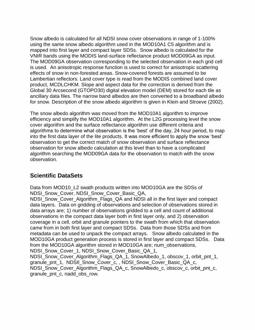
Occurrence of ice on inland water bodies is relevant to study of climate change so an ice or snow covered ice on inland water bodies’ algorithm is included in the algorithm. Ice or snow covered lake ice is detected using the snow algorithm applied specifically to inland water bodies. The lake ice product is provided so that the technique and difficulties of detecting lake ice can be investigated and evaluated by the community. Inland water bodies are mapped by setting a QA algorithm bit flag.
Aqua specific processing The Terra and Aqua MODIS instruments are very similar in design and performance, except for Aqua MODIS band 6 in which the majority of detectors are non-functional (MCST, 2014). In the Aqua MODIS band 6 (1.6 µm) focal plane about 75% of the detectors are non-functional, thus band 6 is useless in the snow algorithm, and band 6 is an integral part of the snow algorithm. In C5 the MYD10_L2 algorithm was revised to use MODIS band 7 (2.12 µm)in place of band 6 and empirically adjusted for band differences; thus the snow detection algorithms for Terra and Aqua were different. The Aqua snow product was considered of lower quality and tended to have more errors compared to MOD10_L2 because of the use of band 7 in C5. The band 6 detector loss has been a factor in the limited use of the Aqua snow products in C5. Recently a Quantitative Image Restoration (QIR) algorithm (Gladkova et al., 2012) was developed and applied to restore the missing Aqua MODIS band 6 data to scientifically usable data for snow detection (http://csdirs.ccny.cuny.edu/csdirs/projects/multi-band-statistical-restoration-aqua). When the MODIS snow algorithm was tested using QIR band 6 data it was found that the output FSC maps are accurate and equal in quality to Terra FSC maps. The QIR algorithm has been integrated in the MYD10_L2 algorithm for C6. Thus the same snow detection algorithm can be run with both Terra and Aqua using band 6 data in C6.
Algorithm Description A brief description of the algorithm approach is given here, however a detailed description can be found in the Algorithm Theoretical Basis Document (ATBD) (http://modis-snow-ice.gsfc.nasa.gov/?c=atbd&t=atbd. The purpose of this description is to explain the flow of the algorithm and the basic technique used to detect snow cover. The output is a NDSI snow cover map with clouds, water bodies and other features included on the map. The algorithm uses as input the MOD02HKM and MOD021KM band radiance data, the MOD03 geolocation data product, and the MOD35_L3 cloud mask. . Inputs to the algorithm are listed in Table 2. The processing flow for a pixel is determined based on the land/water mask. Land and inland water bodies in daylight are processed for snow detection or ice/snow on water detection. MODIS radiance data is checked for nominal quality and converted to TOA reflectance. (Specifics of L1B processing and

documentation can be found at the MODIS Calibration Support Team (MCST) web page http://mcst.gsfc.nasa.gov/) Table 2. MODIS Terra and Aqua data product inputs to the MODIS snow algorithm.
ESDT Long Name Data Used
MOD02HKM
MODIS/Terra Calibrated Radiances 5-Min L1B Swath 500m
Radiance for MODIS bands 1 (0.645 μm) 2 (0.865 μm) 4 (0.555 μm) 6 (1.640 μm)
MYD02HKM
MODIS/Aqua Calibrated Radiances 5-Min L1B Swath 500m
Radiance for MODIS bands 1 (0.645 μm) 2 (0.865 μm) 4 (0.555 μm) QIR 6 (1.640 μm)
MOD021KM
MODIS/Terra Calibrated Radiances 5-Min L1B Swath 1km
Radiance for MODIS bands 31 (11.03 μm )
MYD021KM
MODIS/Aqua Calibrated Radiances 5-Min L1B Swath 1km
Radiance for MODIS bands 31 (11.03 μm )
MOD03
MODIS/Terra Geolocation Fields 5-Min L1A Swath 1km
Land/Water Mask Solar Zenith Angle Latitude Longitude Geoid Height
MYD03
MODIS/Aqua Geolocation Fields 5-Min L1A Swath 1km
Land/Water Mask Solar Zenith Angle Latitude Longitude Geoid Height
MOD35_L2
MODIS/Terra Cloud Mask and Spectral Test Results 5-Min L2 Swath 250m and 1km
Unobstructed Field of View Flag Day/Night Flag
MYD35_L2
MODIS/Aqua Cloud Mask and Spectral Test Results 5-Min L2 Swath 250m and 1km
Unobstructed Field of View Flag Day/Night Flag

Snow typically has very high visible (VIS) reflectance and very low reflectance in the shortwave infrared (SWIR), a characteristic used to detect snow by distinguishing snow and most cloud types. Snow cover is detected using the NDSI ratio of the difference in VIS and SWIR reflectance; NDSI = ((band 4-band 6) / (band 4 + band 6)) A pixel with NDSI > 0.0 is considered to have some snow present. A pixel with NDSI <= 0.0 is snow free land surface. The NDSI is effective at detecting snow cover on the landscape when skies are clear and viewing geometry and solar illumination are good. Snow cover always has an NDSI >0 but not all surface features with NDSI > 0 are snow cover. Some surface features e.g. salt pans, or cloud contaminated pixels at edges of cloud, can have NDSI > 0 and be erroneously detected as snow cover, which results in a snow commission error, detecting snow where there is no snow. Snow commission errors are frequently associated with cloud fringes. To alleviate snow commission errors several data screens based on snow spectral features or other characteristics are applied in the algorithm. The screens are used to reverse snow cover detection or are used to flag uncertain snow cover detection. Snow omission errors occur infrequently. In the algorithm the NDSI is calculated for all land and inland water bodies in daylight, then the data screens are applied to snow detections. All the data screens are applied to each snow pixel. Applying all the data screens to a pixel allows for more than one data screen to be set for a snow commission error or uncertain snow detection. A snow pixel that fails any single data screen will be reversed to not snow and since all the data screens are applied more than a single QA algorithm bit flag may be set. The same data screens are applied to land and inland water pixels. Inland water bodies are mapped with bit 0 of the algorithm bit flags. The cloud mask, ocean mask, and night mask are laid on the NDSI snow cover to make a thematic map of snow cover. The NDSI value is output for all land and inland water pixels.
Data Screens Applied A pixel determined to have some snow present, a snow pixel, is subjected to the following series of screens to alleviate snow commission errors and flag uncertain snow detections. The first screen is a low visible reflectance screen. There must be greater than a minimal amount of reflectance for the algorithm to be run. Snow typically has high VIS reflectance and low SWIR reflectance however the amount of reflectance in any band and the difference in reflectance between bands varies with viewing conditions and surface features. Screens function to detect reflectance relationships atypical of snow and are applied to either reverse a snow detection to a no snow or other decision, or to flag the snow as possibly not snow. Bounding conditions of too low reflectance or too great reflectance are also set by screens. Each screen has a bit flag in the QA algorithm flags SDS (described later in QA section) that is set to on if a screen was failed. Users can extract specific bit flags for analysis. Low VIS reflectance screen

If the VIS reflectance from MODIS band 2 is ≤ 0.10 or band 4 is ≤ 0.11 then a pixel fails to pass this screen. If a pixel is failed a “no decision” is the result This screen is tracked in bit 1 of the NDSI_Snow_Cover_Algorithm_Flags_QA. Low NDSI screen Pixels detected with snow cover in the 0.0 < NDSI < 0.10 are reversed to a no snow result and bit 2 of the NDSI_Snow_Cover_Algorithm_Flags_QA is set. That bit flag can be used to find where a snow cover detection was reversed to not snow. (See Section “Interpretation of Snow Cover Detection Accuracy, Uncertainty and Errors” for explanation of this screen.) Estimated surface temperature and surface height screen There is a dual purpose for this estimated surface temperature linked with surface height screen. It is used to alleviate snow commission errors on low elevations that appear spectrally to be similar to snow but are too warm to be snow. It is also used to flag snow detections on high elevations that are warmer than expected for snow. If snow is detected in a pixel at height < 1300 m and that pixel has an estimated band 31
brightness temperature (BT) ≥ 281 K that snow detection is reversed to not snow and bit
3 is set in the NDSI_Snow_Cover_Algorithm_Flags_QA. If snow is detected in a pixel at
height ≥ 1300 m and with estimated band 31 brightness temperature (BT) ≥ 281 K that
snow detection is flagged as unusually warm by setting bit 3 in the NDSI_Snow_Cover_Algorithm_Flags_QA High SWIR reflectance screen The purpose of this screen is to prevent non-snow features that appear similar to snow to be detected as snow but also to allow snow detection in situations where snow cover SWIR reflectance is anomalously high. This screen has two thresholds settings for different situations. Snow typically has SWIR reflectance less than about 0.20 however, in some situations, e.g. low sun angle, snow can have higher reflectance. If a snow
pixel has a SWIR reflectance in range of 0.25 < SWIR ≤ 0.45 it is flagged as unusually
high for snow and bit 4 of NDSI_Snow_Cover_Algorithm_Flags_QA is set. If a snow pixel has SWIR reflectance > 0.45 it is reversed to not snow and bit 4 of NDSI_Snow_Cover_Algorithm_Flags_QA is set. Solar zenith screen Low illumination conditions exist at solar zenith angles > 70° which is a challenging situation for snow cover detection. A solar zenith mask of > 70° is made by setting bit 7 of NDSI_Snow_Cover_Algorithm_Flags_QA. This mask is set across the entire swath. Night is defined as the solar zenith angle ≥ 85° and pixels are mapped as night.

Lake Ice Algorithm The lake ice, snow covered ice detection algorithm is the same as the NDSI snow cover algorithm. Inland water bodies are tracked by setting bit 0 of NDSI_Snow_Cover_Algorithm_Flags_QA. Users can extract or mask inland water bodies in the NDSI_Snow Cover output using that inland water bit flag. This algorithm uses the basic assumption that a water body is deep and clear and therefore it absorbs all of the solar radiation incident upon it. Water bodies with high turbidity or algal blooms or other conditions of relatively high reflectance from the water may be erroneously detected as snow/ice covered.
Cloud Masking The Unobstructed Field of View (UFOV) cloud mask flag from MOD35_L2 is used to mask clouds. The 1 km cloud mask is applied to the four corresponding 500 m pixels. If the cloud mask flags “certain cloud” then the pixel is masked as cloud. If the cloud mask flag is set “confident clear”, “probably clear” or “uncertain clear” it is interpreted as clear in the algorithm.
Abnormal pixel condition rules If MODIS L1B data is missing in any of the bands used in the algorithm, that pixel is set to “missing data” and is not processed. Unusable L1B data are processed as a no decision result.
Quality Assessment Data A revised approach to quality assessment is applied in C6. A basic QA value is reported and the data screens applied in the algorithm are reported as bit flags. The basic QA value is a qualitative estimate of the algorithm result for a pixel based on L1B input data and solar zenith data. The algorithm bit flags are new and can be used to investigate results for all pixels processed. The basic QA value is initialized to best value and is adjusted based on the quality of the MOD02HKM input data and the solar zenith angle screen. If the MOD02HKM radiance data is outside the range of 5-100% TOA but still usable, the QA value is set to
good. If the solar zenith angle is in range of 70° ≤ solar zenith angle 85° the QA is set
to okay, which indicates increased uncertainty in results because of low illumination. If input data is unusable the QA value is set to other. Conditions for a poor result are not

defined. For features that are masked, e.g. night and ocean the same mask values used in the snow cover data arrays are used. The NDSI_Snow_Cover_Algorithm_Flags_QA is a bit flag array of data screen results applied in the algorithm. By examining the bit flags a user can determine if a snow cover result was changed to a not snow result by a screen or screens, or if a snow covered pixel has certain screens set to on indicative of an uncertain snow detection. The screens and bit flags have dual purpose, some flag where snow detection was reversed or flag snow detection as uncertain. More than one data screen can be on for a snow detection reversal or for uncertain snow detection. The data screens are described in the algorithm section and interpretation of them is discussed in the Interpretation of Snow Cover Detection Accuracy, Uncertainty and Errors section. The inland water flag should be used for analysis of the inland water snow/ice cover result in the algorithm.
Scientific Data Sets
NDSI_Snow_Cover NDSI_Snow_Cover is reported in the range of 0-100% with other results or features identified by unique values. The structure and partial list of local attributes and data content of the SDS are listed in Table 3. An example of the NDSI_Snow_Cover and MODIS imagery for a swath is shown in Figure 2. Snow and ice cover on freshwater bodies is a product within the M*D10 product. Snow/ice cover on inland water bodies, is also mapped using the same range of values as the NDSI_Snow_Cover. Inland water bodies have a value of 237 unless snow or ice was detected. The inland water flag is stored in bit 0 of the NDSI_Snow_Cover_Algorithm_Flags_QA; it can be used to map inland water bodies in the swath.

Figure 2. MODIS C6 NDSI Snow Cover. Terra MODIS acquisition of 10 January 2003, 1750 UTC. False color image of MOD02HKM bands 1,4,6 as RGB, left image; in this band combination snow appears in hues of yellow to blackish-yellow on the landscape. MOD10_L2 C6 NDSI_Snow_Cover product, right image, with snow cover shown as color scaled map with clouds and ocean and night masks.
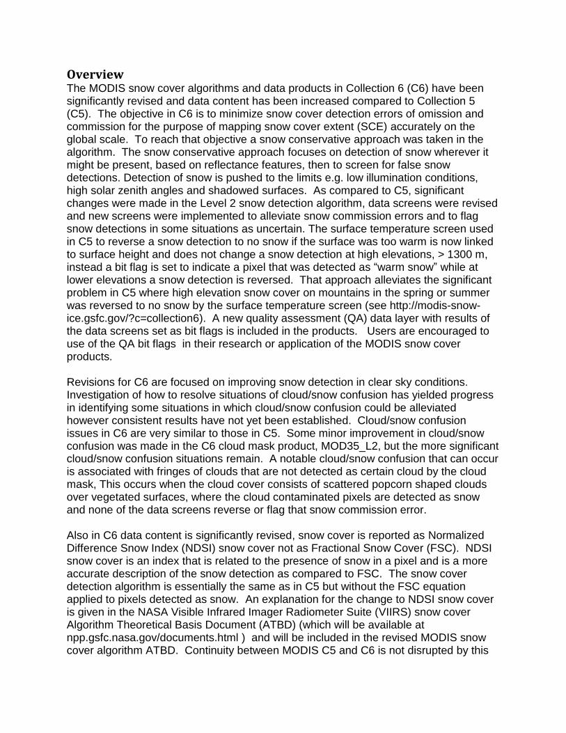
Figure 3. MOD10_L2 C6 snow cover data product. Terra MODIS acquisition of 10 January 2003, 1750 UTC. The four data arrays in the product are; NDSI_Snow_Cover (upper left), algorithm QA bit flags (upper right), basic QA values (lower right) and NDSI data for the swath (lower left). A select combination of algorithm QA bit flags is shown. A user can select an individual bit flag or various combinations of bit flags for their use. Table 3. Definition and partial listing of local attributes of the NDSI_Snow_Cover SDS
SDS name NDSI_Snow_Cover
Data type DFNT_UINT8

Number of dimensions 2
Dimensions--HDF order-- 4060 2708 (AlongTrack, CrossTrack)
Number of local attributes 14
Local Attributes
Attribute name DATA TYPE Data
long_name DFNT_CHAR8 NDSI snow cover, 500m
units DFNT_CHAR8 none
valid_range DFNT_UINT8 0 100
_FillValue DFNT_UINT8 255
Key: DFNT_CHAR8 0-100=NDSI snow 200=missing data 201=no decision 211=night 237=inland water 239=ocean 250=cloud 254=detector saturated 255=fill
NDSI_Snow_Cover_Basic _QA A basic estimate of the quality of the algorithm result for a pixel is reported in this SDS. The quality estimate is given as a value for each pixel processed; an example is shown in Fig. 3. Local attributes are listed in Table 4. The purpose of the basic QA is to allow a user to easily visualize the general quality of the NDSI_Snow_Cover. In depth analysis/evaluation of the NDSI_Snow_Cover should utilize the algorithm specific bit flags QA data. . Table 4. Definition and partial local attributes listing of the NDSI_Snow_Cover_Basic_QA SDS.
SDS name NDSI_Snow_Cover_Basic_QA
Data type DFNT_UINT8
Number of dimensions 2
Dimensions--HDF order--
4060 2708 (AlongTrack, CrossTrack)
Number of local attributes
5
Local Attributes
Attribute name DATA TYPE Data
long_name DFNT_CHAR8 NDSI snow cover general quality value

units DFNT_CHAR8 none
valid_range DFNT_UINT8 0 4
_FillValue DFNT_UINT8 255
Key: DFNT_CHAR8 0=best, 1=good, 2=ok, 3=poor-not used, 211=night, 239=ocean, 255=unusable L1B data or no data
NDSI_Snow_Cover_Algorithm_Flags_QA Algorithm bit flags are set for data screen results. The data screens serve two purposes, 1) they indicate why a snow detection was reversed to not snow, and 2) are a QA flag for uncertain snow detection or challenging viewing condition. More than one bit flag may be set because all data screens are applied to a pixel, The inland water mask is also set by a bit flag set to support analysis of inland waters for snow/ice cover. Bits for the data screens are set to on if the screen was failed. An example of some of the bit flags and combinations of bit flags is shown in Fig. 3. Many combinations of bit flags may be set. A user can investigate any bit flag or combinations of bit flags. Table 5 lists local attributes. Table 5. Definition and local attributes listing of the NDSI_Snow_Cover_Algorithm_Flags_QA SDS.
SDS name NDSI_Snow_Cover_Algorithm_Flags_QA
Data type DFNT_UINT8
Number of dimensions
2
Dimensions--HDF order--
4080 2708 (AlongTrack, CrossTrack)
Number of local attributes
6
Local Attributes
Attribute name DATA TYPE Data
long_name DFNT_CHAR8 NDSI snow cover algorithm flags
units DFNT_CHAR8 none
format DFNT_CHAR8 bit flag
valid_range DFNT_UINT8 0 254
_FillValue DFNT_UINT8 255
Key: DFNT_CHAR8 bit on means: bit 0: inland water flag bit 1: low visible screen failed, reversed snow detection bit 2: low NDSI screen failed,

reversed snow detection bit 3: combined temperature and height screen failed, snow reversed because too warm and too low. This screen is also used to flag a high elevation too warm snow detection, in this case the snow detection is not changed but this bit is set. bit 4: too high SWIR screen and applied at two thresholds: QA bit flag set if band6 TOA > 25% & band 6 TOA <=45%, indicative fo unusual snow condition, or snow commission error; snow detection reversed if band6 TOA > 45% bit 5 : spare bit 6 : spare bit 7 : solar zenith screen, indicates increased uncertainty in results
NDSI An NDSI value is calculated for all land and inland water pixels in daylight in the swath. An example of the NDSI data is shown in Fig. 3. A listing of local attributes is in Table 6. Table 6. Definition and partial listing of local attributes of the NDSI SDS.
SDS name NDSI
Data type DFNT_INT16
Number of dimensions 2
Dimensions--HDF order-- 4060 2708 (AlongTrack, CrossTrack)
Number of local attributes 4
Local Attributes
Attribute name DATA TYPE Data
long_name DFNT_CHAR8 Raw NDSI (Normalized Difference Snow Index) layer
units DFNT_CHAR8 none

valid_range DFNT_INT16 0 10000
Scale_factor DFNT_FLOAT32 0.00010000
Latitude and Longitude Latitude and longitude data at 5 km resolution are provided for geolocation and browse product generation purposes. The latitude and longitude data correspond to a center pixel of a 5 km by 5 km block of pixels in the snow SDSs. The mapping relationship of geolocation data to the snow data is specified in the global attribute StructMetadata.0. The mapping relationship was created by the HDF-EOS SDPTK toolkit during production. Geolocation data is mapped to the snow data with an offset = 5 and increment = 10. The first element (1,1) in the geolocation SDSs corresponds to element (5,5) in NDSI_Snow_Cover SDS; the algorithm then increments by 10 in the cross-track or along-track direction to map geolocation data. Table 7. Definition and local attributes listing of Latitude and Longitude SDSs.
SDS name Latitude
Data type DFNT_FLOAT32
Number of dimensions 2
Dimensions--HDF order-- 406 271
Number of local attributes 5
Local Attributes
Attribute name DATA TYPE Data
long_name DFNT_CHAR8 Coarse 5 km resolution latitude
units DFNT_CHAR8 degrees
valid_range DFNT_FLOAT32 -90.00000 90.00000
_FillValue DFNT_FLOAT32 -999.0000
Source DFNT_CHAR8 M*D03 geolocation product; data read from center pixel in 5 km box
SDS name Longitude
Data type DFNT_FLOAT32
Number of dimensions 2
Dimensions--HDF order-- 406 271
Number of local attributes 5
Local Attributes
Attribute name DATA TYPE Data
long_name DFNT_CHAR8 Coarse 5 km resolution longitude
units DFNT_CHAR8 degrees
valid_range DFNT_FLOAT32 -180.0000 180.0000
_FillValue DFNT_FLOAT32 -999.0000
Source DFNT_CHAR8 MOD03 geolocation product; data read from center pixel in 5 km box
Interpretation of Snow Cover Detection Accuracy, Uncertainty and Errors A focus of research and applications has been on monitoring snow cover extent (SCE), onset of snow cover, duration, and melt over a year or years for hydrologic or climate change studies. Revisions to the MODIS snow detection algorithms and products for C6 were strongly influenced by published investigations. Accurate detection of SCE is the parameter most studied in relation to climate change (e.g., see Derksen and Brown, 2012). Continued investigation and evaluation of algorithm results coupled with study of published results has lead to revisions in the C6 algorithm and data product that reduce snow commission and omission errors, and provide users with a greater amount of data and QA information to evaluate, analyze and interpret. Snw cover is detectable with good accuracy when illumination conditions are near ideal, skies are clear, and several centimeters or more of snow are present on the landscape. Snow cover can occur on many different landscapes,including forests, plains and mountains, and under all types of viewing conditions. Viewing conditions change from day to day and across the landscape. The diversity of situations where snow may be found makes it challenging to develop a globally applicable snow cover detection algorithm. Though challenging, the MODIS snow algorithm was designed to identify snow globally in all situations. The NDSI technique for snow detection has proved to be a robust indicator of snow around the globe as evidenced by the numerous investigators who have used the MODIS snow products and reported accuracy statistics in the range of 88-93%, and who have derived season snow maps from the snow cover products. (See listing of publications at http://modis-snow-ice.gsfc.nasa.gov/?c=publications). For a revised explanation of the NDSI snow cover algorithm theory see the NASA VIIRS Snow Cover ATBD (Riggs and Hall, 2015, under review) which gives a detailed explanation of the algorithm. The MODIS and VIIRS snow cover algorithms both use the NDSI snow detection algorithm, albeit adjusted for sensor and input data product differences. The MODIS snow cover ATBD will be updated but the VIIRS ATBD (Riggs and Hall, 2015) will probably be available sooner. The major changes in the MODIS C6 snow products (as compared to C5) are 1) there is no ‘binary’ snow covered area (SCA) SDS and 2) there is no fractional snow cover (FSC). The FSC has been replaced by the NDSI_Snow_Cover. Algorithm specific data screen results, and the calculated NDSI data are ouput. These changes provide more data and great flexibility to a user for accurate usage of the data products.

The binary SCA algorithm was abandoned because it was restricted to the NDSI range of 0.4 to 1.0, with a special test for combination of NDSI in the 0.1 to 0.4 range and NDVI to increase sensitivity so snow detection in forested landscapes. However, that
algorithm prevented detection of snow cover that had NDSI values in the 0 ≤ NDSI
0.4 range on any landscape. If a user wants to make a binary SCA from the C6 product they can set their own NDSI threshold for snow using the NDSI_Snow_Cover or the NDSI data or a combination of those data. The NDSI snow cover algorithm is designed to detect snow cover across the entire range of NDSI values from 0.0 - 1.0. This is the theoretically possible range for snow. By using this entire range the ability to map snow in many situations is increased, notably in situations where reflectance is relatively low and snow has a low but positive NDSI value. NDSI_Snow_Cover replaces the FSC of C5. The FSC was calculated based on an empirical relationship that was based on the extent of snow cover in Landsat TM 30 m pixels that corresponded to a MODIS 500 m pixel. Change to the NDSI snow cover algorithm is explained in Riggs and Hall (2015) which is the VIIRS snow cover ATBD. The NDSI_Snow_Cover is essentially the same as the FSC in C5. A user can calculate FSC from NDSI_Snow Cover by applying the FSC equations of FSC = (-0.01 + (1.45 *
NDSI)) * 100.0 for 0.0 ≤ NDSI ≤ 1.0 for Terra or Aqua MODIS data. Platform unique
FSC equations are not needed in C6 because the QIR technique is used to restore Aqua MODIS band 6 data which allows the same equation to be used with C6 data (see AQUA Specific Processing section for description of the QIR algorithm applied to Aqua MODIS data). In C5 the FSC equation was unique to each platform because of the loss of Aqua MODIS band 6 data forced the use of band 7 in the snow cover algorithm. Analysis of MOD10 C5 snow cover maps, with emphasis on snow cover omission and commission errors observed and reported in the literature prompted changes in the snow detection algorithm for C6. The algorithm logic is as follows: snow cover always has an NDSI > 0 but not all features with NDSI > 0 are snow. Snow detection is applied to all land pixels in a swath then snow detections are screened to reverse possible snow commission errors, flag uncertain snow detections and set QA flags. Results of the data screens are set as bit flags in the NDSI_Snow_Cover_Algorithm_Flags_QA. All the data screens are applied so it is possible that more than one flag is set for a pixel. Some situations associated with snow commission errors and possible ways to interpret the algorithm bit flags are discussed in following subsections. Surface Temperature and Height Screen A surface temperature screen was applied in the C5 snow mapping algorithm to reverse all snow detections that were thought to be too warm to be snow. A decision on any

pixel detected as snow cover and having an estimated surface temperature >283 K was reversed to no snow. That temperature screen was successful at greatly reducing the occurrence of erroneous snow cover in warm regions of the world and along warm coastal regions. However, it was discovered that the temperature screen also caused significant snow omission errors. Snow omission errors in spring and summer on snow covered mountain ranges could be very large as the seasonal surface temperature increased above 283 K. The effect of the temperature screen on mapping of snow cover on the Sierra Nevada from 1 May to 1 August 2010 is exhibited at http://modis-snow-ice.gsfc.gov/?c=collection6. Snow omission errors were around 10% at start of that time period then rose to near 90% at the end. It is probable that snow omission errors associated with seasonally increasing temperatures occurred on some mountain ranges depending on the climate they are located. Our investigation found that the surface temperature screen caused significant snow cover omission errors on some mountain ranges in the melt season but it was also effective at preventing snow commission errors over warm surfaces in situations were the spectrally based screens did not block snow commission errors. In C6 the surface temperature screen is combined with surface elevation and used in two ways. This combined screen reverses snow cover detection on low elevation < 1300 m surfaces that are too warm for snow and the algorithm QA bit flag is set. Snow cover detection at
≥1300 m on a surface that is too warm for snow is not reversed but that snow cover
detection is flagged as too warm by setting the algorithm QA bit flag. The effectiveness of the surface temperature and height screen varies as the surface changes over seasons. It is effective at reversing snow commission errors of some surface features, and cloud contaminated pixels over some landscapes when the surface is warm, However when the surface is below the threshold temperature, or cloud contamination lowers the estimated surface temperature this screen is not effective. A surface feature that is spectrally similar to snow, for example the Bonneville Salt Flats will have snow detection reversed by this screen when the surface is warm but not reversed when the surface is cold and snow free in the winter. Low Illumination or Low Reflectance Low solar illumination conditions occurring when the solar zenith angle is > 70.0° and near to the day/night terminator are a challenge to snow detection. Low reflectance situations in which reflectance is <~30% across the visible bands is also a challenge for snow detection. Low reflectance across the VIS and SWIR bands can result in relatively small differences between the VIS and SWIR bands and give an NDSI > 0.. Very low visible reflectance is cause for increased uncertainly in detection of snow cover. Investigation and discussion with some users who encountered errors associated with low reflectance surface conditions resulted in setting a low reflectance limit in the algorithm. If VIS reflectance is too low a pixel is set to no decision and the low VIS data screen bit flag is set. This is considered a low limit to accurate detection of snow cover on the landscape. Low reflectance associated with low illumination, landscape shadowed by clouds or terrain, and unmapped water bodies or inundated
landscape can exhibit reflectance characteristics similar to snow and thus be erroneously detected as snow by the algorithm. The NDSI is calculated for those no decision results so a user can see the NDSI value by using the low visible QA bit flag and NDSI data. Low NDSI Low VIS reflectance situations where the difference between VIS and SWIR is very small can have very low positive NDSI values. Those low positive NDSI results can occur where visible reflectance is low or high and where the associated SWIR is low or high but slightly lower than the VIS so that the NDSI is a very low positive value In our analysis of many such situations we found that very uncertain snow detections or snow commission errors were common when the NDSI was 0.0 ≤ NDSI < 0.1. Based on that analysis a low NDSI screen is applied, If NDSI is <0.1 a snow detection is reversed to not snow and the low NDSI bit 2 flag is set in the QA. A user can use that bit flag to determine where snow detections were reversed and their NDSI value. High SWIR Reflectance Unusually high SWIR reflectance may be observed in some snow cover situations, from some types of clouds not masked as certain cloud or from non-snow surface features. A SWIR screen is applied at two thresholds to either reverse a possible snow commission error or flag snow detection with unusually high SWIR. A user can check this bit flag to find where uncertain snow cover detections occurred or where snow detection one was reversed to not snow. Cloud and Snow Confusion Cloud and snow confusion in C6 is similar to C5 albeit there is a slight reduction in occurrence of cloud/snow confusion that we observer in the C6 cloud mask which is attributed to revisions made in the cloud mask algorithm. The snow cover algorithm reads the “Unobstructed FOV Quality Flag” from the MOD35_L2 product which has four values cloudy, uncertain, probably clear and confident clear. If the cloud mask has cloudy for a pixel then that pixel is set to cloud in the snow algorithm, the other three values are interpreted as clear. Cloud/snow confusion emanates from two cloud mask algorithm results; the cloud mask fails to detect a cloud as certain cloud, or the cloud mask detects snow as certain cloud. In situations where the cloud mask fails to identify a cloud, and the cloud reflectance characteristics are similar to snow, it may be detected as snow which will result in a commission error. In situations where the cloud mask flags snow cover as certain cloud then a snow omission error occurs. Snow commission errors associated with the periphery of clouds where the subpixel clouds are not detected as certain cloud is a cloud contamination problem in the snow cover algorithm and may result in snow commission errors. Cold clouds that appear to have some ice content and that appear in shades of yellow, are very similar to snow in RGB display of MODIS bands, 1, 4 and 6. In addition, if they are self shadowed by other parts of the cloud, they can pass as not certain cloud in the cloud mask algorithm, and can then be detected as snow in the snow algorithm. Snow commission errors

associated with self shadowed clouds and their periphery is frequently seen in situations of scattered, popcorn like cloud formations over vegetated landscapes, as shown in Fig. 4. In these types of cloud cover conditions the subpixel contaminated clouds and self shadowed clouds are spectrally indistinct from snow in the algorithm. Those cloud cover conditions are transient from day to day. Such transient snow commission errors can possibly be filtered temporally or spatially or by a combination of filters.
Figure 4. Cloud/snow confusion example. MODIS swath of 13 July 2003 (2003194) 1835 UTC imaging central Canada, left image RGB of bands 1,4, and 6, Hudson Bay top right of swath, Great Slave Lake, left center, Cloud type and formation over vegetation in which snow commission errors can occur are shown in image subsets marked by red square in left image, shown in right images, top RGB of bands 1,4 and 6 and NDSI_Snow_Cover, bottom right image. The orange circle highlights a cloud

formation where snow commission error occurs on both self shadowed cloud and cloud periphery. Cloud/snow confusion along the periphery of a snow covered region, notably if the snow cover is thin or sparse and the sky is clear the cloud mask may flag the snow cover as certain snow. This situation can be seen associated with swaths of snow cover dropped by storms crossing the Great Plains where snow on the periphery of the snow covered region is flagged as certain cloud by the cloud mask . In the C4 algorithm this cloud/snow confusion situation was investigated and it was found that the snow was detected as cloud by only a single visible cloud test of the several cloud spectral tests applied in that processing path. We found that by examining the cloud mask algorithm processing path and results of all cloud spectral tests applied that the cloud mask could be reinterpreted as clear in that specific situation and the snow could then be correctly detected. That reinterpretation test was partially effective at resolving this specific cloud/snow confusion situation however in global application of that test inconsistencies in results were found, thus that test was not applied in C5. Use of the MOD35_L2 algorithm processing path flags and individual cloud spectral tests still holds promise for resolving some snow/cloud confusion situations and is being investigated. Lake Ice Because of the importance of lake ice cover formation, duration and ice out date to study of climate change a lake ice detection algorithm is implemented in C6 to map ice or snow and ice covered lakes and rivers. The lake ice detection algorithm is similar to that in C5 but is better integrated into the overall algorithm flow. Lake ice cover is included in the NDSI_Snow_Cover data . Inland water bodies are mapped using the MODIS land/water mask in the MOD03 product. The lake ice algorithm is the same as the NDSI snow detection algorithm. Inland water bodies are mapped in bit 0 of the algorithm QA flags data so that bit can be used for analysis of lake ice. Visual analysis of MODIS imagery and MOD10_L2 products acquired during boreal winter when lakes are frozen reveals that snow/ice covered lakes are detected with 90-100% accuracy. Disappearance of lake ice also appears to be detected with a high accuracy. During ice free season changes in physical characteristics of a lake can greatly affect the accuracy of the algorithm. Sediment loads, high turbidity, aquatic vegetation and algae blooms change the reflectance characteristics and may frequently be the cause of erroneous lake or river ice cover detection in the spring or summer. A lake ice specific algorithm should be developed for Collection 7. Lake ice is included in the NDSI snow cover so that a spatially coherent image of a snow covered landscape can be seen. A user can extract the inland water mask from bit 0 of the NDSI_Snow_Cover_Algorithm_Flags_QA data for use in analysis or to apply as a static water mask.

Bright Surface Features Surface features such as salt flats, bright sands, or sandy beaches that have VIS and SWIR reflectance characteristics similar to snow maybe detected as snow cover based solely on the NDSI value thus resulting in errors of commission. Screens specifically for bright surfaces were not developed for C6 but the screens in C6 can reduce occurrence of snow commission errors in some situations, e.g. a low elevation, too warm surface can be blocked by the surface temperature and height screen. These surface features are static so a user could mask or flag these surfaces relevant to their research or application. Land/water Mask and Geolocation Uncertainty In MODIS C6 the land/water mask is derived from the UMD 250m MODIS Water Mask data product (UMD Global Land Cover Facility http://glcf.umd.edu/data/watermask/description.shtml). Location of lakes and rivers is greatly improved compared to the land/water mask used in C5. Users will probably notice an increase in the number of lakes mapped, especially in regions of small lakes, e.g. northern Minnesota to the Northwest Territories, and that many larger rivers are more continuous. The improved quality of the land water mask is seen through all product levels. The UMD 250 m Water Mask was converted to a 500 m seven class land/water mask for use in the production of MODIS products in C6. That was done to maintain continuity in the land/water mask used in all the land products in C5 to C6 but with greatly improved accuracy in location of water bodies resulting from the UMD 250 Water Mask (http://landweb.nascom.nasa.gov/QA_WWW/forPage/MODIS_C6_Water_Mask_v3.pdf) Geolocation accuracy in C6 remains similar to C5 (Wolfe and Nishihama,2009; Wolfe, 2006). There will be some uncertainty in geolocation of land/water mask features but within an expected range. Geolocation uncertainty through the processing levels to level 3 may be observed in MOD10A1, notable in how water bodies are mapped from day to day, and is commented on in the MOD10A1 section. Antarctica The Antarctic continent is nearly completely ice and snow covered year round, with very little annual variation though some variation can occur on the Antarctic Peninsula, The snow algorithm is run for Antarctica without adjustment unique to Antarctica. The snow cover map may show areas of no snow cover, which is a very obvious error. That error is related to the great difficulty in identifying clouds over Antartica’s ice/snow cover. The similarity in reflectance and lack of thermal contrast between clouds and ice/snow cover and thermal inversions are challenges to accurate snow/cloud discriminaton. In situations where the cloud mask fails to identify certain cloud the snow algorithm assumes a cloud free view and either identifies the surface as not snow covered or identifies the cloud as snow. In either case the result is wrong. Scrolling through global browse imagery of MOD10_L2 reveals many instances of snow free patches on Antarctica. Though the MOD10_L2 and MOD10A1 products are generated on Antarctica, they must be carefully scrutinized for accuracy and quality. In the MOD10C1

product Antarctica is masked as 100% snow cover to generate a visually good representation of Antarctica in the global product.
MOD10GA New in C6 is the daily level 2-G gridded snow cover product MOD10GA. All the MOD10_L2 swath products from a day are mapped into this product which is then used as input for the MOD10A1 daily snow product. The MOD10GA is an intermediate product in the series of snow products that is not archived at the NSIDC DAAC thus is not available for order.
Algorithm Description The MODAPS built a generic gridding algorithm for many of the MODIS data products to create the L2G daily gridded data products (Wolfe et al., 1999). The Earth is divided into an array of 36 x 18, longitude by latitude, tiles, about 10°x10° in size in the Sinusoidal projection. The gridding algorithm maps MODIS Level-2 swath products in to a tile of the grid and creates the relevant gridding projection data structures in the product. A snow product version of that gridding algorithm was built to generate the MOD10GA product in C6. During development of the algorithm it was realized that coding and production efficiency through the series of snow algorithms and products could be improved by moving the snow cover observation selection algorithm and snow albedo algorithm from the MOD10A1 product generation process to the MOD10GA product generation process, so they were integrated into MOD10GA product generation process. The MOD10GA observation selection algorithm uses several criteria to select the ‘best’ observation of a day from the MODIS swaths that cover a location. The observation selection criteria used are solar elevation, distance from nadir, observation cover (pixel coverage in a grid cell of the projection), to map an observation into the first data layer. Thus the ‘best’ observation for each product is based only on those criteria so that the observation selected is nearest local solar noon time, nearest the orbit nadir track and with most coverage in a grid cell, which is considered the best sensor view of the surface on a day relevant to snow cover detection. Those ‘best’ observations are mapped into the product as the first layer of data. This strategy results in a contiguous mapping of swaths with a weave or checkerboard pattern along stitched together swath edges within a tile. That weave pattern is sometimes apparent where cloud cover changed between acquisition times of overlapping swaths. Observations from other swaths that may be mapped into that same grid cell are stored in compact format as a one dimension array in run length encoded format to reduce data volume. Pointers to the orbit and granule (swath) from which each observation was selected from are stored as SDSs. Those pointers can be linked to the names of input granules in the ArchiveMetadata to determine the date and time of acquisition of each observation.
Snow albedo is calculated for all NDSI snow cover observations in range of 1-100% using the same snow albedo algorithm used in the MOD10A1 C5 algorithm and is mapped into first layer and compact layer SDSs. Snow albedo is calculated for the VNIR bands using the MODIS land-surface reflectance product MOD09GA as input. The MOD09GA observation corresponding to the selected observation in each grid cell is used. An anisotropic response function is used to correct for anisotropic scattering effects of snow in non-forested areas. Snow-covered forests are assumed to be Lambertian reflectors. Land cover type is read from the MODIS combined land cover product, MCDLCHKM. Slope and aspect data for the correction is derived from the Global 30 Arcsecond (GTOPO30) digital elevation model (DEM) stored for each tile as ancillary data files. The narrow band albedos are then converted to a broadband albedo for snow. Description of the snow albedo algorithm is given in Klein and Stroeve (2002). The snow albedo algorithm was moved from the MOD10A1 algorithm to improve efficiency and simplify the MOD10A1 algorithm. At the L2G processing level the snow cover algorithm and the surface reflectance algorithm use different criteria and algorithms to determine what observation is the ‘best’ of the day, 24 hour period, to map into the first data layer of the lite products. It was more efficient to apply the snow ‘best’ observation to get the correct match of snow observation and surface reflectance observation for snow albedo calculation at this level than to have a complicated algorithm searching the MOD09GA data for the observation to match with the snow observation.
Scientific DataSets Data from MOD10_L2 swath products written into MOD10GA are the SDSs of NDSI_Snow_Cover, NDSI_Snow_Cover_Basic_QA, NDSI_Snow_Cover_Algorithm_Flags_QA and NDSI all in the first layer and compact data layers. Data on gridding of observations and selection of observations stored in data arrays are; 1) number of observations gridded to a cell and count of additional observations in the compact data layer both in first layer only, and 2) observation coverage in a cell, orbit and granule pointers to the swath from which that observation came from in both first layer and compact SDSs. Data from those SDSs and from metadata can be used to unpack the compact arrays. Snow albedo calculated in the MOD10GA product generation process is stored in first layer and compact SDSs. Data from the MOD10GA algorithm stored in MOD10GA are; num_observations, NDSI_Snow_Cover_1, NDSI_Snow_Cover_Basic_QA_1, NDSI_Snow_Cover_Algorithm_Flags_QA_1, SnowAlbedo_1, obscov_1, orbit_pnt_1, granule_pnt_1, NDSIl_Snow_Cover_c, , NDSI_Snow_Cover_Basic_QA_c, NDSI_Snow_Cover_Algorithm_Flags_QA_c, SnowAlbedo_c, obscov_c, orbit_pnt_c, granule_pnt_c, nadd_obs_row.

MOD10A1 The daily gridded snow cover product contains the ‘best’ NDSI_Snow Cover, snow albedo and QA observation selected from all the MOD10_L2 swaths mapped into a grid cell on the Sinusoidal projection in the MOD10GA. The product is a tile of approximately 1200x1200 km (10°x10°) area on the Sinusoidal projection (modis-land.gsfc.nasa.gov/MODLAND_grid.html). Also included is a pointer to the swath granule from which an observation came that can be used to extract the time of acquisition. An example of the MOD10A1 NDSI_Snow_Cover map and algorithm QA bit flags is shown in Figure 5.
Figure 5. MOD10A1 C6 snow product. The daily NDSI_Snow_Cover product (left image) and NDSI_Snow_Cover_Algorithm_Flags_QA (right) for 2003014 tile h11v04 covering a western Great Lakes region.
Algorithm Description The observation selection algorithm and snow albedo algorithm were moved to the MOD10GA product generation process (see Section MOD10GA). That selection algorithm picks the ‘best’ observation from the one to many MOD10_L2 observations that were acquired of the surface from all swaths of a day. The snow albedo algorithm was also moved to production of MOD10GA and is described in Section MOD10GA. The MOD10A1 algorithm in C6 reads the first layer SDSs from MOD10GA, calculates some descriptive QA statistics, and writes out those SDSs and descriptive metadata and also copies some metadata from MOD10GA into in the MOD10A1.

Scientific Data Sets
NDSI_Snow_Cover This is the NDSI snow cover that was detected in the MOD10_L2 algorithm, then gridded by the MOD10GA algorithm and selected as the ‘best’ observation for a grid cell for the day, then subsequently written into this SDS. The list of local attributes and data content of the SDS are listed in Table 7. Table 7. Structure and local attributes listing of NDSI_Snow_Cover
SDS name NDSI_Snow_Cover
Data type DFNT_UINT8
Number of dimensions 2
Dimensions--HDF order-- 2400 2400
Local Attributes
Attribute name DATA TYPE Data
long_name DFNT_CHAR8 NDSI snow cover from best observation of the day
units DFNT_CHAR8 none
valid_range DFNT_UINT8 0, 100
Missing_value DFNT_UINT8 200
_FillValue DFNT_UINT8 255
Key: DFNT_CHAR8 0-100=NDSI snow, 200=missing data, 201=no decision, 211=night, 237=inland water, 239=ocean, 250=cloud, 254=detector saturated, 255=fill
NDSI_Snow_Cover_Basic_QA A general estimate of the quality of the algorithm result for a pixel is reported in this SDS. This QA estimate was made in the MOD10_L2 algorithm then passed to the MOD10GA where ‘best’ observation was selected which was then written into this SDS. The structure and list of local attributes and data content are listed in Table 8. Table8. Structure and local attributes listing of NDSI_Snow_Cover_Basic_QA
SDS name NDSI_Snow_Cover_Basic_QA
Data type DFNT_UINT8
Number of dimensions 2

Dimensions--HDF order--
2400 2400
Local Attributes
Attribute name DATA TYPE Data
long_name DFNT_CHAR8 NDSI snow cover general quality value
units DFNT_CHAR8 none
valid_range DFNT_UINT8 0 4
_FillValue DFNT_UINT8 255
Key: DFNT_CHAR8 0=best, 1=good, 2=ok, 3=poor-not used, 4=other-not used, 211=night, 239=ocean, 255=unusable L1B or no data
NDSI_Snow_Cover_Algorithm_Flags_QA Bit flags set for data screen results and for inland water mask in the MOD10_L2 algorithm. This data corresponds to the ‘best’ observation selected in MOD10GA algorithm which was then written into this SDS. The list of local attributes and data content of the SDS are listed in Table 9. Table 9 Local attributes listing of NDSl_Snow_Cover_Algorithm_Flags_QA
SDS name NDSI_Snow_Cover_Algorithm_Flags_QA
Data type DFNT_UINT8
Number of dimensions
2
Dimensions--HDF order--
2400 2400
Local Attributes
Attribute name DATA TYPE Data
long_name DFNT_CHAR8 NDSI snow cover algorithm bit flags
units DFNT_CHAR8 none
format DFNT_CHAR8 bit flag
valid_range DFNT_UINT8 0 254
_FillValue DFNT_UINT8 255
Key: DFNT_CHAR8 bit on means: bit 0: inland water flag bit 1: low visible screen failed,

reversed snow detection bit 2: low NDSI screen failed, reversed snow detection bit 3: combined temperature and height screen failed, snow reversed because too warm and too low. This screen is also used to flag a high elevation too warm snow detection, in this case the snow detection is not changed but this bit is set. Bit 4 : too high SWIR screen and applied at two thresholds: QA bit flag set if band6 TOA > 25% & band6 TOA <=45%, indicative of unusual snow condition, or snow commission error snow detection reversed if band6 TOA > 45% bit 5 : spare bit 6 : spare bit 7 : solar zenith screen, indicates increased uncertainty in results
NDSI This is the NDSI that was calculated in the MOD10_L2 algorithm, then gridded by the MOD10GA algorithm and selected as the ‘best’ observation for a grid cell for the day, then subsequently written into this SDS. The list of local attributes and data content of the SDS are listed in Table 10. Table 10. Local attributes of NDSI.
SDS name NDSI
Data type DFNT_INT16
Number of dimensions 2
Dimensions--HDF order-- 2400 2400
Local Attributes
Attribute name DATA TYPE Data
long_name DFNT_CHAR8 Raw NDSI
units DFNT_CHAR8 none
valid_range DFNT_INT16 0, 10000
_FillValue DFNT_INT16 0

scale_factor DFNT_FLOAT32 0.0001000000
Snow_Albedo_Daily_Tile The snow albedo as calculated by the snow albedo algorithm is stored in this SDS. The snow albedo map corresponds to snow cover extent in the NDSI_Snow_Cover SDS. Snow albedo is reported in the 0 –100 range and non-snow features are mapped using unique data values. The list of local attributes and data content of the SDS is shown in Table 11. Table 11. Structure and local attributes listing of Snow_Albedo_Daily_Tile
SDS name Snow_Albedo_Daily_Tile
Data type DFNT_UINT8
Number of dimensions
2
Dimensions--HDF order--
2400 2400
Local Attributes
Attribute name DATA TYPE Data
long_name DFNT_CHAR8 Snow albedo of the corresponding snow cover observation
units DFNT_CHAR8 none
valid_range DFNT_UINT8 0 100
_FillValue DFNT_UINT8 255
Missing_value DFNT_UINT8 250
Key: DFNT_CHAR8 0-100=snow albedo, 101=no_decision, 111=night, 125=land, 137=inland water, 139=ocean, 150=cloud, 151=cloud detected as snow, 250=missing,, 251=self_shadowing, 252=landmask mismatch, 253=BRDF_failure, 254=non-production_mask

orbit_pnt Pointer to the orbits of the swaths that were mapped into each grid cell is stored in this SDS. The pointers, point by index to the listing of orbit numbers in the metadata object “ORBITNUMBERARRAY” written in ArchiveMetadata.0. Table 12. Structure and local attributes listing of orbit_pnt
SDS name orbit_pnt
Data type DFNT_UINT8
Number of dimensions
2
Dimensions--HDF order--
2400 2400
Local Attributes
Attribute name DATA TYPE Data
long_name DFNT_CHAR8 Orbit pointer for observation
units DFNT_CHAR8 none
valid_range DFNT_UINT8 0 15
_FillValue DFNT_UINT8 255
granule_pnt The pointer to the swaths that were mapped into each grid cell is stored in this SDS. The pointers correspond to the listing of granule pointers in the metadata object “GRANULEPOINTERARRAY” written in ArchiveMetadata.0. A positive granule pointer means that the swath was mapped into the tile. More granules (swaths) are staged for input than actually overlap with a tile, only the granules that overlap the tile, identified by a positive pointer value are mapped into the tile. In order to determine the swath origin of a cell observation, link the pointers in GRANULEPOINTERARRAY to granule data and time in GRANULEBEGINNINGDATETIMEARRAY by index, then the date and beginning time string can be extracted. Table 13. Structure and local attributes listing of granule_pnt
SDS name granule_pnt
Data type DFNT_UINT8
Number of dimensions
2
Dimensions--HDF order--
2400 2400
Local Attributes

Attribute name DATA TYPE Data
long_name DFNT_CHAR8 Granule pointer for observation
units DFNT_CHAR8 none
valid_range DFNT_UINT8 0 254
_FillValue DFNT_UINT8 255
Interpretation of Snow Cover and Snow Albedo Accuracy, Uncertainty and Errors The NDSI snow cover originates from the MOD10_L2 algorithm with only a single observation (pixel) from the one to several that may have been acquired from satellite overpasses during a day selected and stored as the ‘best’ observation of the day. Discussion regarding the interpretation and uncertainty of the NDSI snow cover is the same as presented in the Interpretation of Snow Cover Accuracy, Uncertainty and Errors section under MOD10_L2. Validation and evaluation of the snow albedo data is ongoing. Snow albedo is estimated to be within 10% of surface measured snow albedo based on studies in the literature (Klein and Stroeve, 2002; Tekeli et al., 2006) and unpublished evaluations. That estimate is based on best conditions, level surface, complete snow cover, for the algorithm however, in conditions difficult to calculate snow albedo, e.g., steep mountain terrain the snow albedo error could be large. Snow albedo specific QA is not reported in C 6 because ways of expressing the QA of the snow albedo result are still being investigated. Evaluation and validation of snow albedo will lead to the definition and setting of QA data. Updates to snow albedo evaluation and validation will be posted on the snow project website. The MODIS BRDF/Albedo product MCD43 may also be of interest for theh study of snow albedo www.umb.edu/spectralmass/terra_aqua_modis/modis_brdf_albedo_product_mcd43. New in C6 is the granule pointer data that points to the swath from which an observation came. The pointer data can be linked to metadata to determine the time of acquisition, start and end time of swath, of every observation. Acquisition time data is the swath beginning and ending times stored in metadata objects. Linking the pointers and metadata is described above in granule_pnt description. The selection algorithm for ‘best’ observation of the day results in a contiguous mapping of adjacent swaths with a weave or stitch pattern along swath edges as shown in Figure 6 That stitch pattern is most apparent where cloud cover changed between acquisition

times of overlapping swaths. There may be a weave of cloud and clear observations in images of the snow cover data. Viewing geometry differences between adjacent swaths may also cause discontinuity in overlap regions.
Figure 6. Example of stitching pattern along overlapping input swaths. The four overlapping input swaths to MOD10A1.A2003014.h11v04.(same tile as shown in Fig. 5) each shown in a different color. Full tile shown on the left with higher resolution image of stitching pattern where three swaths overlap shown on the right. Geolocation error may be apparent in the product due to uncertainty in L2 geolocation and gridding and projecting the swath data to the Sinusoidal projection from day to day. That type of geolocation wobble is commonly observed in the location of freshwater bodies over time. In a composite of tile over the course of several consecutive days the position of a lake shoreline may shift by one or more cells in the horizontal or vertical directions each day resulting in a blurred outline of the lake. For example, a composite of the inland water mask, bit 0 in the NDSI_Snow_Cover_Algorithm_Flags_QA, from tile h11v04 for five days 7-11 January 2003 is shown in Fig. 7. The southern shoreline of Lower Red Lake in MN and smaller lakes to the south shown in Fig.7 appear blurred in the composite due to day to day geolocation wobble.
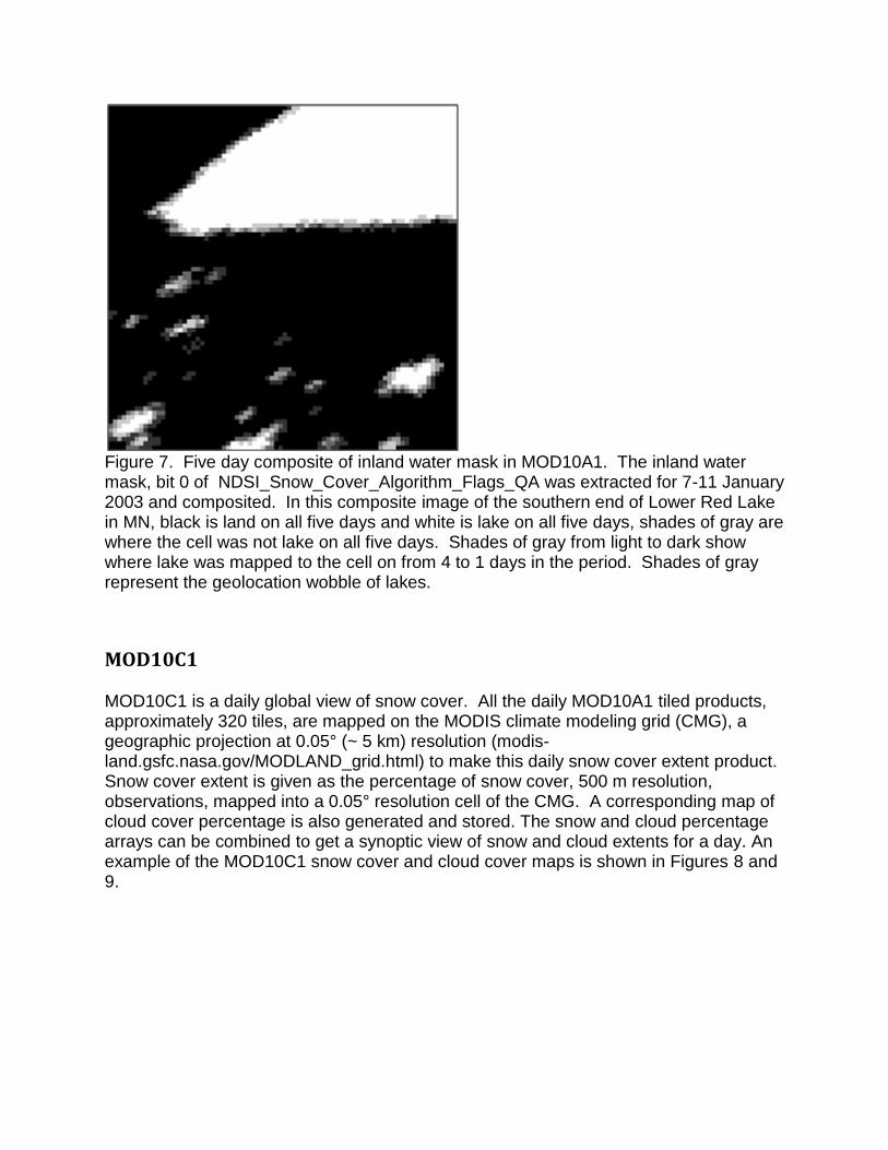
Figure 7. Five day composite of inland water mask in MOD10A1. The inland water mask, bit 0 of NDSI_Snow_Cover_Algorithm_Flags_QA was extracted for 7-11 January 2003 and composited. In this composite image of the southern end of Lower Red Lake in MN, black is land on all five days and white is lake on all five days, shades of gray are where the cell was not lake on all five days. Shades of gray from light to dark show where lake was mapped to the cell on from 4 to 1 days in the period. Shades of gray represent the geolocation wobble of lakes.
MOD10C1 MOD10C1 is a daily global view of snow cover. All the daily MOD10A1 tiled products, approximately 320 tiles, are mapped on the MODIS climate modeling grid (CMG), a geographic projection at 0.05° (~ 5 km) resolution (modis-land.gsfc.nasa.gov/MODLAND_grid.html) to make this daily snow cover extent product. Snow cover extent is given as the percentage of snow cover, 500 m resolution, observations, mapped into a 0.05° resolution cell of the CMG. A corresponding map of cloud cover percentage is also generated and stored. The snow and cloud percentage arrays can be combined to get a synoptic view of snow and cloud extents for a day. An example of the MOD10C1 snow cover and cloud cover maps is shown in Figures 8 and 9.
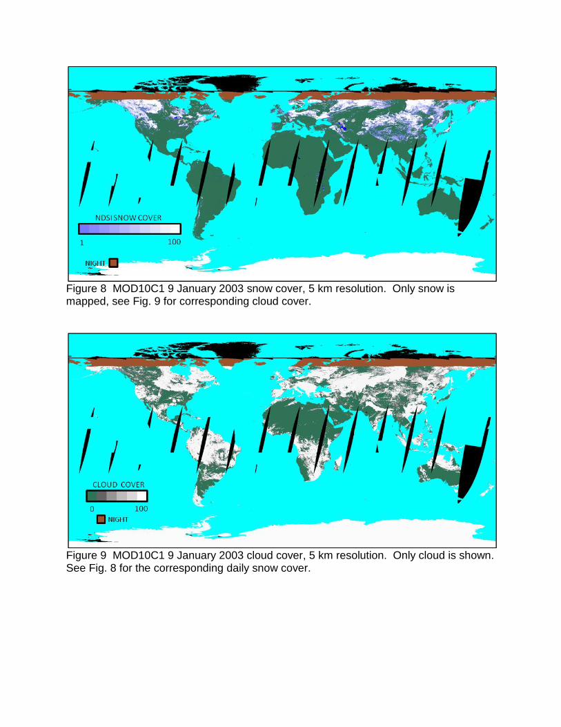
Figure 8 MOD10C1 9 January 2003 snow cover, 5 km resolution. Only snow is mapped, see Fig. 9 for corresponding cloud cover.
Figure 9 MOD10C1 9 January 2003 cloud cover, 5 km resolution. Only cloud is shown. See Fig. 8 for the corresponding daily snow cover.

Algorithm Description A binning algorithm is used to determine snow cover extent, cloud cover extent, and associated quality assessment in a CMG grid cell. MOD10A1 data inputs are binned and tallied; outputs for a grid cell are determined by the percentage of counts of observations, snow or cloud, mapped in the cell based on total land extent in the grid cell. Inputs to the algorithm are listed in Table 14. The input NDSI snow cover data is translated to a snow or not snow flag that is counted in the binning algorithm to determine the percentage of snow observations in a cell that is output as fraction of cell covered by snow. The NDSI snow cover 0-100% is interpreted as a binary snow flag to tally observations of snow mapped in a grid cell. Cloud observations are interpreted and tallied using that method. The binning algorithm generates the snow and cloud cover maps based the total number of observations of a feature, e.g. snow, cloud, snow-free land, etc. and total number of land observations mapped into a cell of the CMG. Lake ice coverage is also included in the snow map. Inland water bodies are determined using the water flag in the snow algorithm flags QA for counting number of water body observations in a grid cell. Observations are tallied for lakes; if the water body has more lake ice observations than open water observations it is interpreted as lake ice with a value of 107 in the output. Lakes that are cloud obscured are output as cloud obscured with a value of 250. Table 14 MODIS data product inputs to the MOD10C1 snow algorithm.
ESDT Long Name Data Used
MOD10A1 “MODIS/Terra Snow Cover Daily L3 Global 500m SIN Grid"
NDSI_Snow_Cover NDSI_Snow_Cover_Basic_QA
A CMG specific land base mask was made for use with the binning algorithm. The 0.05° land mask was derived from the University of Maryland 1km global land cover data set (http://glcf.umiacs.umd.edu/data/landcover/index.shtml). If a CMG cell contains 12% or greater land then it is considered land and analyzed; if less than 12% it is considered ocean. That threshold was selected as a balance that minimized snow errors along coasts yet was sensitive to mapping snow along coasts. The extent of clear views in a cell is presented as an index of the amount of surface observed in the grid cell. This index is called the clear index and is intended to provide users with an estimate of percentage of all observations that were clear. This index indicates how much of the surface in a cell was observed, clear sky, and can be used to assess quality of the snow percentage in a grid cell. The clear index (CI) is essentially 100 minus the percentage of cloud in a cell, though it is calculated based on observation counts in the algorithm code. The CI values are stored in the "Day_CMG_Clear_Index" SDS. A high CI is indicative of clear conditions and a low CI is

indicative of a lot of cloud cover and that snow percentage may not be a good estimate because of the cloud cover obscuring all or parts of a cell.
Polar darkness extent is determined based on the latitude of the CMG cell nearest the equator that is full of night observations. All CMG cells poleward from that latitude are filled as night. Polar darkness is determined this way so that a neat demarcation of night and day is shown in the CMG. Antarctica has been masked as 100% snow covered. That masking was done to improve the visual quality of data display. This product is not applicable to snow mapping in Antarctica. During austral summer some coastal regions, mainly the Antarctic Peninsula, may be snow free for a brief period of time. Study of those or other areas of Antarctica should use the MOD10_L2 product that is of higher resolution and contain more data and information on accuracy and error. A global mask showing where the occurrence of snow is extremely unlikely, e.g. the Amazon, the Sahara, Great Sandy Desert, is applied at the end of the algorithm to eliminate probable erroneous snow cover detection. The source of erroneous snow in those regions is the MOD10_L2 product where erroneous snow detection occurs and is carried forward through the processing levels to the CMG. At the CMG level the use of this extremely unlikely snow mask eliminates erroneous snow from the masked regions but allows it in regions where snow may be a rare event.
Scientific Data Sets
Day_CMG_Snow_Cover The percentage of snow-covered land mapped in the CMG cell is given in the "Day_CMG_Snow_Cover" SDS. Snow cover percentage is the fraction of snow covered land based on the entire amount of land mapped in the CMG grid cell. No attempt was made to interpret snow cover possibly obscured by cloud. Percentage of snow is reported in the range of 0-100%. Table 15 Local attributes for Day_CMG_Snow_Cover
SDS name Day_CMG_Snow_Cover
Data type DFNT_UINT8
Number of dimensions 2
Dimensions--HDF order-- 3600, 7200
Local Attributes
Attribute name DATA TYPE Data
long_name DFNT_CHAR8 Daily snow extent, global at 5km
units DFNT_CHAR8 none
coordsys DFNT_CHAR8 latitude, longitude
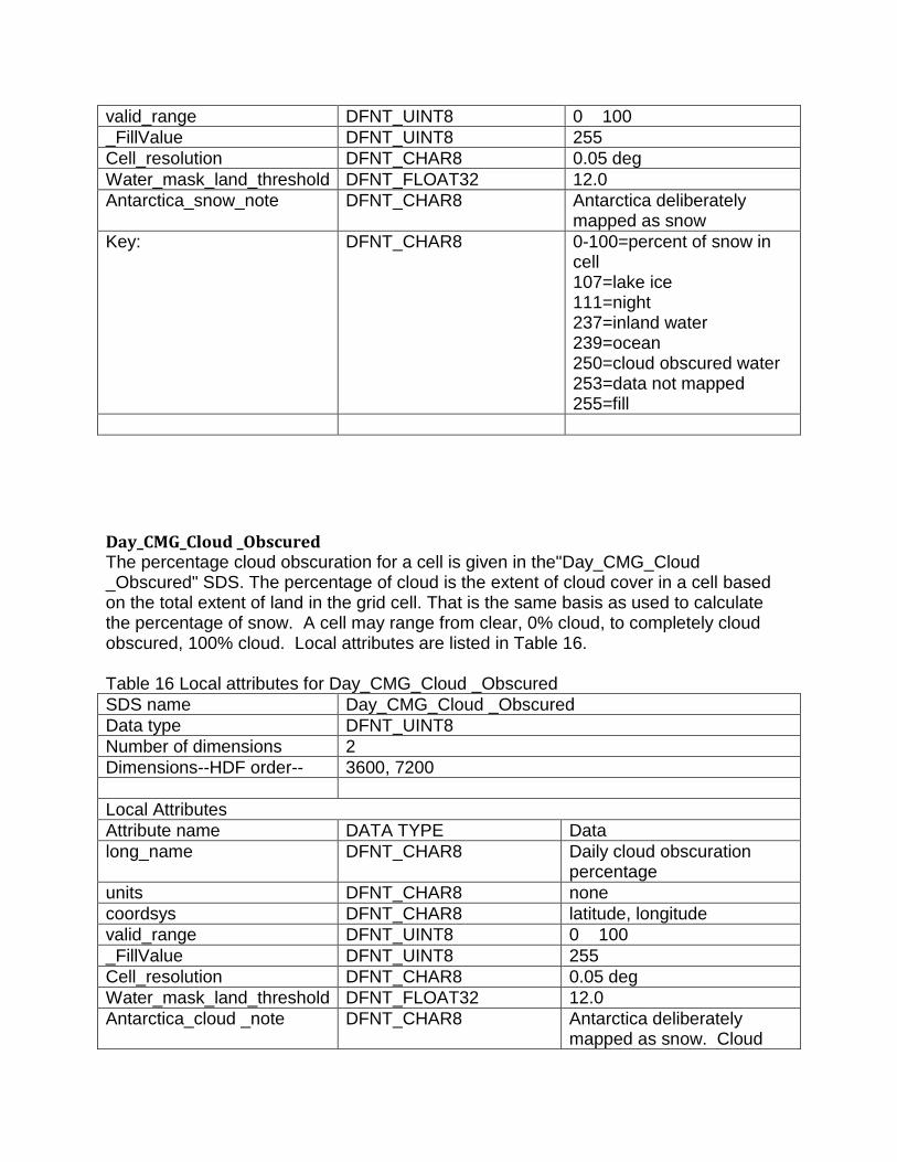
valid_range DFNT_UINT8 0 100
_FillValue DFNT_UINT8 255
Cell_resolution DFNT_CHAR8 0.05 deg
Water_mask_land_threshold DFNT_FLOAT32 12.0
Antarctica_snow_note DFNT_CHAR8 Antarctica deliberately mapped as snow
Key: DFNT_CHAR8 0-100=percent of snow in cell 107=lake ice 111=night 237=inland water 239=ocean 250=cloud obscured water 253=data not mapped 255=fill
Day_CMG_Cloud _Obscured The percentage cloud obscuration for a cell is given in the"Day_CMG_Cloud _Obscured" SDS. The percentage of cloud is the extent of cloud cover in a cell based on the total extent of land in the grid cell. That is the same basis as used to calculate the percentage of snow. A cell may range from clear, 0% cloud, to completely cloud obscured, 100% cloud. Local attributes are listed in Table 16. Table 16 Local attributes for Day_CMG_Cloud _Obscured
SDS name Day_CMG_Cloud _Obscured
Data type DFNT_UINT8
Number of dimensions 2
Dimensions--HDF order-- 3600, 7200
Local Attributes
Attribute name DATA TYPE Data
long_name DFNT_CHAR8 Daily cloud obscuration percentage
units DFNT_CHAR8 none
coordsys DFNT_CHAR8 latitude, longitude
valid_range DFNT_UINT8 0 100
_FillValue DFNT_UINT8 255
Cell_resolution DFNT_CHAR8 0.05 deg
Water_mask_land_threshold DFNT_FLOAT32 12.0
Antarctica_cloud _note DFNT_CHAR8 Antarctica deliberately mapped as snow. Cloud

value set to 252
Key: DFNT_CHAR8 0-100=percent of cloud in cell 107=lake ice 111=night 237=inlandwater 239=ocean 250=cloud obscured water 252=Antarctica mask 253=data not mapped 255=fill
Day_CMG_Clear_Index An index of the snow cover being a good or poor estimate relative to cloud cover is stored in this SDS. The CI ranges from 0 -100%. Local attributes listed in Table 17. Table 17 Local attributes for Day_CMG_Clear _Index
SDS name Day_CMG_Clear_Index
Data type DFNT_UINT8
Number of dimensions 2
Dimensions--HDF order-- 3600, 7200
Local Attributes
Attribute name DATA TYPE Data
long_name DFNT_CHAR8 Clear index for the daily snow map
units DFNT_CHAR8 none
coordsys DFNT_CHAR8 latitude, longitude
valid_range DFNT_UINT8 0 100
_FillValue DFNT_UINT8 255
Mask_value 254
Cell_resolution 0.05 deg
Water_mask_land_threshold(%) 12.00000
Antarctica_clear_index_note Antarctica deliberately mapped as snow. Clear index set to 100
Key: DFNT_CHAR8 0-100=clear index value, 107=lake ice, 111=night, 237=inland water, 239=ocean,

250=cloud obscured water, 253=data not mapped, 255=fill
Snow_Spatial_QA The basic QA value for a grid cell is the most frequent basic QA value associated with the MOD10A1 observations mapped into a cell. The binning algorithm returns the most frequent QA value; if there is a tie in QA values then the highest QA value of the tied values is reported in the Snow_Spatial_QA SDS. Local attributes are listed in Table 18. Table 18 Local attributes for Snow_Spatial_QA SDS
SDS name Snow_Spatial_QA
Data type DFNT_UINT8
Number of dimensions 2
Dimensions--HDF order-- 3600, 7200
Local Attributes
Attribute name DATA TYPE Data
long_name DFNT_CHAR8 General QA of data in grid cell
units DFNT_CHAR8 none
coordsys DFNT_CHAR8 latitude, longitude
valid_range DFNT_UINT8 0 4
_FillValue DFNT_UINT8 255
Cell_resolution 0.05 deg
Water_mask_land_threshold(%) 12.00000
Antarctica_QA _note Antarctica delibertly maped as snow. QA value set to 252.
Key: DFNT_CHAR8 0=best 1=good, 2=ok, 3=poor, 4=other 252=Antarctica mask 253=not mapped 254=no retrieval 255=fill
Interpretation of Snow Cover Accuracy, Uncertainty and Errors

The daily CMG gives a synoptic view of snow cover extent. The snow cover and cloud cover data and optionally the clear index data array can be combined to make a synoptic view of snow cover with the cloud mask overlaid. Snow cover and cloud cover are produced in separate data arrays so that a user may interpret or combine the data relevant to their research or applications. Understanding the propagation of sources of possible snow and cloud errors in the MO10_L2 products to the CMG is useful for determining how to interpret and possibly filter errors or uncertain conditions. Snow errors in MOD10C1 are propagated from the MOD10_L2 to the MOD10A1 product then into the MOD10C1, see the MOD10_L2 section for discussion of possible errors. Snow commission errors are typically associated with cloud cover thus snow errors on any day may appear associated with the cloud cover. A user should consider how to interpret and make best use the snow cover data or combine it with the cloud cover data for their purposes Because of the great difficulty in discriminating between clouds and snow over Antarctica in the level-2 snow detection and cloud mask algorithms (see earlier discussion in MOD10_L2 section) the quality of the data product is low and therefore, Antarctica is masked as 100% snow cover. Though masking improves the visual quality of the image it excludes scientific study of Antarctica. To reduce erroneous snow mapping in regions of the world that climatologically should never have snow, a snow “impossible” mask was created and applied in the algorithm. The purpose of this mask is to improve the synoptic quality of the product. A drawback of application of the mask is that unusual snowfall events can be blocked in this product. The MOD10_L2 and MOD10A1 products should be used to investigate unusual snowfall events.
MOD10A2 This product provides the maximum extent of snow cover, and the days on which snow cover was observed over an eight day period. The maximum snow extent is where snow was observed on at least one day during the period. Days in the period on which snow was observed are mapped as a bit flag chronology of observed snow cover. Cloud cover is not included but if there was persistent cloud cover on all eight days then cloud cover is reported for a grid cell. An example of the eight-day snow cover map is shown in Fig. 10. An eight day period is used because that is the period of near repeat ground track of the MODIS satellites (Masuoka et al., 1998) not for any cryospheric science reason.
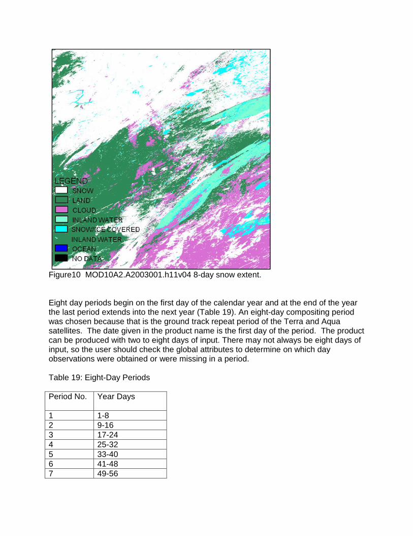
Figure10 MOD10A2.A2003001.h11v04 8-day snow extent. Eight day periods begin on the first day of the calendar year and at the end of the year the last period extends into the next year (Table 19). An eight-day compositing period was chosen because that is the ground track repeat period of the Terra and Aqua satellites. The date given in the product name is the first day of the period. The product can be produced with two to eight days of input. There may not always be eight days of input, so the user should check the global attributes to determine on which day observations were obtained or were missing in a period. Table 19: Eight-Day Periods
Period No. Year Days
1 1-8
2 9-16
3 17-24
4 25-32
5 33-40
6 41-48
7 49-56

8 57-64
9 65-72
10 73-80
11 81-88
12 89-96
13 97-104
14 105-112
15 113-120
16 121-128
17 129-136
18 137-144
19 145-152
20 153-160
21 161-168
22 169-176
23 177-184
24 185-192
25 193-200
26 201-208
27 209-216
28 217-224
29 225-232
30 233-240
31 241-248
32 249-256
33 257-264
34 265-272
35 273-280
36 281-288
37 289-296
38 297-304
39 305-312
40 313-320
41 321-328
42 329-336
43 337-344
44 345-352
45 353-360
46 361-368*
*Includes 2 or 3 days from next year, depending on leap year

Algorithm Description The algorithm composites eight days of MOD10A1 tiles to map the maximum snow extent for the period and tracks the days that snow was observed chronologically across a bit field. Inputs to the algorithm are listed in Table 20. The eight days of observations for a cell are read and if snow was found for any day in the period then that cell is mapped as snow in the "Maximum_Snow_Extent" data array. The MOD10A1 NDSI snow cover is filtered for the purpose of reducing possible snow commission errors and giving a more spatially consistent snow extent map by interpreting NDSI snow cover in the 1- 10 range as uncertain snow and not counting it for maximum snow cover. If no snow is found in the period then the type of observation that occurred most often is mapped as the observation for the period. For example, if there were five snow free land, and three cloud observations, the cell will be reported as snow free land. The algorithm is biased to selecting clear views for the period using only the clear views to determine the composite observation. An exception to that logic is made if all eight days are observed with cloud, if all eight days are cloud then the result it cloud. The logic minimizes cloud cover extent in that a cell must to be cloud obscured for all eight days of observation to be labeled as cloud. If a composite observation is not determined then the output is a no decision, to catch unexpected conditions. Lake ice is also composited using the same algorithm. A chronology of observed snow is tracked as a bit field in the "Eight_Day_Snow_Cover"data array. On days that snow is observed the bit corresponding to that day, eight days across the byte from right to left, is set to on. The input days are ordered from first to last day including placing any missing days in the order. Table 20 MODIS data product inputs to the MOD10A2 snow algorithm.
ESDT Long Name Data Used
MOD10A1 “MODIS/Terra Snow Cover Daily L3 Global 500m SIN Grid"
NDSI_Snow_Cover_
The algorithm will generate a product if there are two to eight days of input available. If there is only a single day of input the product will not be produced. All eight days of input may sometimes not be available due to data acquisition or data product production problems. The algorithm was designed to run will with fewer than eight days so that the

data acquired could be processed even if one to six days of data is unavailable. Days used as input are identified in the global attributes.
Scientific Data Sets
Maximum_Snow_Extent The maximum snow extent for the period depicts where snow was observed on one or more days in the period. Maximum snow extent and other features observed are mapped in this SDS. Local attributes are listed in Table 21. Table 21 Local Attributes for the "Maximum_Snow_Extent" SDS
SDS name Maximum_Snow_Extent
Data type DFNT_UINT8
Number of dimensions 2
Dimensions--HDF order-- 2400 2400
Local Attributes
Attribute name DATA TYPE Data
long_name DFNT_CHAR8 Maximum snow extent over the 8-day period
units DFNT_CHAR8 none
valid_range DFNT_UINT8 0 254
_FillValue DFNT_UINT8 255
Cell_area (km^2) DFNT_FLOAT32 0.2146587
Max_snow_area (km^2) DFNT_FLOAT32 443282.0
Key: DFNT_CHAR8 0=missing data, 1=no decision, 11=night, 25=no snow, 37=lake, 39=ocean, 50=cloud, 100=lake ice, 200=snow, 254=detector saturated, 255=fill
Eight_Day_Snow_Cover Input files are ordered chronologically in the algorithm and if snow was observed the corresponding day bit is set. Across a byte the days are ordered from right to left, bit 0 corresponds to day 1 of the eight-day period, bit 1 corresponds to day 2 of the eight-day

period... bit 7 corresponds to day 8 of the eight day period. Local attributes are listed in Table 21. Table 22 Local Attributes for the "Eight_Day _Snow_Cover" SDS
SDS name Eight_Day _Snow_Cover
Data type DFNT_UINT8
Number of dimensions 2
Dimensions--HDF order-- 2400 2400
Local Attributes
Attribute name DATA TYPE Data
long_name DFNT_CHAR8 Eight day snow cover chronobyte
units DFNT_CHAR8 bit
valid_range DFNT_UINT8 0 255
_FillValue DFNT_UINT8 0
Key: DFNT_CHAR8 Snow occurrence in chronological order. Day in period ordered as 87654321 corresponds to bit order of 76543210. Bit value of 1 means snow was observed. Bit value of 0 means snow was not observed.
Interpretation of Snow Cover Accuracy, Uncertainty and Errors The eight day snow cover extent is intended to provide a map of maximum snow cover extent during that time period and to show on which days snow cover was observed. Typically the accuracy is similar to the MOD10A1 product but may be lower because compositing of the daily snow commission errors over eight days can increase the percentage of error spatially and temporally despite the filter applied to reduce errors. Accuracy and errors from the MOD10A1 inputs, which originated in the MOD10_L2, are propagated into the eight-day snow cover maps. Errors associated with snow/cloud confusion from the MOD10_L2 product can be seen in the eight-day snow maps. Snow errors of commission are typically manifest as snow in locations and seasons where snow is impossible or very unlikely. Errors accumulate from each day and the errors

probably occur in different locations on different days which increase the spatial extent of error in the eight-day snow map.
MOD10C2 This product gives a global view of maximum snow cover extent for an eight day period. All the eight-day MOD10A2 tiled products, approximately 320 tiles, are mapped and binned on the MODIS climate modeling grid (CMG), a geographic projection 0.05° resolution (modis-land.gsfc.nasa.gov/MODLAND_grid.html) to make the maximum snow cover extent map (Fig. 11). Maximum snow cover extent with corresponding persistent cloud cover, clear index and a QA data arrays are in the product.

Figure 11. MOD10C2 for 1-8 January 2003. Maximum snow cover extent (top) for the eight-day period and corresponding map of persistent cloud cover (bottom). The eight-day snow cover is the fraction of observations mapped into the CMG grid cell that were snow on any one of the eight days.
Algorithm Description The MOD10C2 algorithm is a revised version of the MOD10C1 algorithm running with the MOD10A2 eight day products as inputs. The MOD10A2 data inputs are mapped, binned and tallied for a grid cell. Results for a cell are determined by the percentage of counts of observations, maximum snow cover or persistent cloud, mapped in the cell based on total land extent in the grid cell. Inputs to the algorithm are listed in Table 23. A binning algorithm is employed to count the data by category, e.g. maximum snow, persistent cloud, night, etc. mapped to a grid cell. As with the MOD10C1 algorithm a clear index of the amount of surface observed in the grid cell is calculated. What the index measures in MOD10C2 is that amount of persistent cloud that was present in a grid cell (eight consecutive days). Any value > 0 means that some fraction of the cell was cloud obscured for eight days. The clear index values are stored in the "Eight_Day_CMG_Clear_Index" SDS. The QA value is determined by a count of valid and invalid values tallied in a grid cell. This simple method of estimating QA is used because there is no QA data generated or stored in the MOD10A2 product. Default QA value is good, A poor QA value is set if the count of invalid data is the majority tally of observations in a grid cell. Antarctica is arbitrarily mapped as permanent snow cover because Antarctica is 99% or greater snow covered. During the summer up to 1% may be snow-free mostly on the Antarctic Peninsula. Mapping Antarctica as always snow-covered was done for aesthetic purposes for producing and viewing a global map. Table 23 MODIS data product inputs to the MOD10C2 snow algorithm.
ESDT Long Name Data Used
MOD10A2 “MODIS/Terra Snow Cover 8-day L3 Global 500m SIN Grid"
Maximum_Snow_Extent
Scientific Data Sets
Eight_Day_CMG_Snow_Cover This SDS is the global map of maximum snow cover extent for the eight-day period. Extent of snow cover observed is expressed as a percentage of maximum snow observations mapped in to the CMG cell. The valid range of snow cover extent is 0-100%. Local attributes are listed in Table 24.
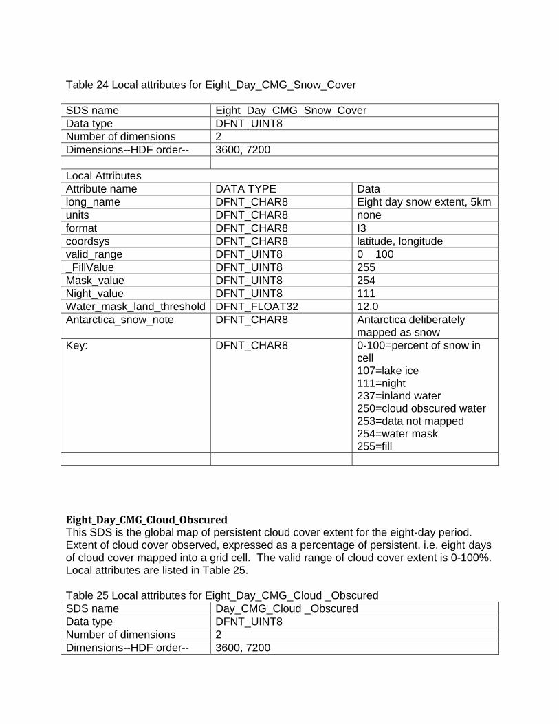
Table 24 Local attributes for Eight_Day_CMG_Snow_Cover
SDS name Eight_Day_CMG_Snow_Cover
Data type DFNT_UINT8
Number of dimensions 2
Dimensions--HDF order-- 3600, 7200
Local Attributes
Attribute name DATA TYPE Data
long_name DFNT_CHAR8 Eight day snow extent, 5km
units DFNT_CHAR8 none
format DFNT_CHAR8 I3
coordsys DFNT_CHAR8 latitude, longitude
valid_range DFNT_UINT8 0 100
_FillValue DFNT_UINT8 255
Mask_value DFNT_UINT8 254
Night_value DFNT_UINT8 111
Water_mask_land_threshold DFNT_FLOAT32 12.0
Antarctica_snow_note DFNT_CHAR8 Antarctica deliberately mapped as snow
Key: DFNT_CHAR8 0-100=percent of snow in cell 107=lake ice 111=night 237=inland water 250=cloud obscured water 253=data not mapped 254=water mask 255=fill
Eight_Day_CMG_Cloud_Obscured This SDS is the global map of persistent cloud cover extent for the eight-day period. Extent of cloud cover observed, expressed as a percentage of persistent, i.e. eight days of cloud cover mapped into a grid cell. The valid range of cloud cover extent is 0-100%. Local attributes are listed in Table 25. Table 25 Local attributes for Eight_Day_CMG_Cloud _Obscured
SDS name Day_CMG_Cloud _Obscured
Data type DFNT_UINT8
Number of dimensions 2
Dimensions--HDF order-- 3600, 7200
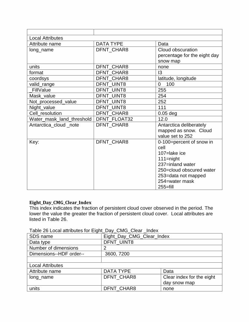
Local Attributes
Attribute name DATA TYPE Data
long_name DFNT_CHAR8 Cloud obscuration percentage for the eight day snow map
units DFNT_CHAR8 none
format DFNT_CHAR8 I3
coordsys DFNT_CHAR8 latitude, longitude
valid_range DFNT_UINT8 0 100
_FillValue DFNT_UINT8 255
Mask_value DFNT_UINT8 254
Not_processed_value DFNT_UINT8 252
Night_value DFNT_UINT8 111
Cell_resolution DFNT_CHAR8 0.05 deg
Water_mask_land_threshold DFNT_FLOAT32 12.0
Antarctica_cloud _note DFNT_CHAR8 Antarctica deliberately mapped as snow. Cloud value set to 252
Key: DFNT_CHAR8 0-100=percent of snow in cell 107=lake ice 111=night 237=inland water 250=cloud obscured water 253=data not mapped 254=water mask 255=fill
Eight_Day_CMG_Clear_Index This index indicates the fraction of persistent cloud cover observed in the period. The lower the value the greater the fraction of persistent cloud cover. Local attributes are listed in Table 26. Table 26 Local attributes for Eight_Day_CMG_Clear _Index
SDS name Eight_Day_CMG_Clear_Index
Data type DFNT_UINT8
Number of dimensions 2
Dimensions--HDF order-- 3600, 7200
Local Attributes
Attribute name DATA TYPE Data
long_name DFNT_CHAR8 Clear index for the eight day snow map
units DFNT_CHAR8 none

format DFNT_CHAR8 I3
coordsys DFNT_CHAR8 latitude, longitude
valid_range DFNT_UINT8 0 100
_FillValue DFNT_UINT8 255
Mask_value 254
Water_mask_land_threshold(%) 12.00000
Antarctica_clear_index_note Antarctica deliberately mapped as snow. Clear index set to 100
Key: DFNT_CHAR8 0-100=clear index value, 107=lake ice, 237=inland water, , 250=cloud obscured water, 253=data not mapped, 254=water mask 255=fill
Snow_Spatial_QA The QA value is determined based on count of valid or invalid data values mapped into a grid cell. Local attributes are listed in Table 27. Table 27 Local attributes for Snow_Spatial_QA SDS
SDS name Snow_Spatial_QA
Data type DFNT_UINT8
Number of dimensions 2
Dimensions--HDF order-- 3600, 7200
Local Attributes
Attribute name DATA TYPE Data
long_name DFNT_CHAR8 Snow cover per cell QA
units DFNT_CHAR8 none
format DFNT_CHAR8 I3
coordsys DFNT_CHAR8 latitude, longitude
valid_range DFNT_UINT8 0 1
_FillValue DFNT_UINT8 255
Mask_value DFNT_UINT8 254
Water_mask_land_threshold(%) 12.00000
Antarctica_QA _note Antarctica deliberately mapped as snow. QA value set to 252.
Key: DFNT_CHAR8 0=good quality, 1=other quality,

252=Antarctica mask, 253=data not mapped 254=ocean mask 255=fill
Interpretation of Snow Cover Accuracy, Uncertainty and Errors A synoptic view of maximum snow extent is given in this product. The maximum snow extent in each grid cell is the fraction of all observations mapped and binned in that cell that had snow cover on at least one day in the eight-day period. Persistent cloud cover, i.e. eight consecutive days of cloud cover, extent is mapped in the cloud obscured data array, which is the fraction of all observations binned in that cell that had persistent cloud cover in the period. Because single day cloud cover is not tracked in this product the clear index should be interpreted as the extent of persistent cloud cover. A clear index of 0 does not mean that there was no obscuring cloud cover in the period; it means that there were not eight consecutive days of cloud cover observed. This index indicates how much of the surface in a cell was persistently cloud covered. Accuracy and error are similar to the MOD10A2 product with,snow detection errors occurring in MOD10_L2 being propagated into the eight-day snow cover product. Snow commission errors are typically the most apparent type of error seen. Probable snow commission errors over eight days may spread in spatial extent and manifest as low percentages of maximum snow fractions in a grid cell. Snow commission errors on the southeastern USA in Fig.11 (zoom to 300+% to see them) are an example of the spread of snow commission errors. Based on experience with the data product, a majority of most probable snow commission errors can be filtered by interpreting snow cover values < 20 to be not snow. However, screening at that leve may block what could be actual snow along the periphery of snow covered regions. No screening for errors is done in the algorithm so a user should analyze the snow cover and interpret it for their use in a way that minimizes probable errors yet makes reasonable use of the product to track maximum snow cover extent. The QA data indicates if the input data are valid or invalid or if special condition like polar darkness existed. The QA value should be interpreted as whether input data value was good or poor.
MOD10CM This is a global, 0.05° resolution monthly mean snow cover extent derived from MODIS daily snow cover extent product MOD10C1. An example of monthly snow cover extent of MOD10CM is shown in Figure 12.

Figure 12. MOD10CM monthly mean snow cover January 2003
Algorithm Description Average snow cover is calculated for each cell in the CMG using the 28 – 31 days of MOD10C1 for the month. Data is filtered so that the most relevant days of snow cover are used to calculate the average and to filter out data that is of low magnitude i.e. low occurrence of snow during the month. The latter filter works to remove some occurrences of erroneous snow from the monthly snow average. The daily snow data is used to compute the monthly average snow cover. A daily cell must have a Clear Index (CI) of > 70% to be included in the average. That filter is applied so that only the clearest of the daily observations are included in the average. (See the MOD10C1 section for description of the CI.) A daily observation contributes to the monthly average for a cell as follows: Daily contribution to monthly mean = 100 * snow%/CI For daily observations that are cloud free the snow contribution to the mean is the observed snow fraction in a grid cell. For daily observations of mixed snow and cloud fractions with a high CI it is assumed that there is some fraction of snow cover obscured by cloud. In that case the daily snow observation is increased in that equation so that the contribution to the monthly mean will be greater than the daily snow observation. For example, a cell has 25% snow cover and the CI = 75 then the cell is determined to
have (25%/75 * 100) = 33% fractional snow cover. Daily observations with a CI ≤ 70 are
assigned either as 100% cloudy, night, missing or no decision. There must be at least one day in the month for each cell with the CI > 70 in order for the mean snow cover to be computed for that cell of the monthly CMG. If that restriction is not met then the cell is reported as no decision. A second filter is applied to the calculated mean fractional snow cover of each cell to filter out those cells in which the magnitude of snow cover is less than 10%. Cells failing the filter are assigned 0% snow for the month. Cells with a low magnitude are considered suspect of being erroneous snow originating in the MOD10_L2 algorithm

and being propagated through the sequence of snow products. The magnitude of snow is calculated as an average snow for all days with snow passing the first filter of CI > 70. For example; cell A has 20 days with CI = 100, 10 days have 100% snow and 10 days have 0% snow, the mean monthly snow = (10 * 100 + 10 * 0)/20 = 50%. The second filter would be calculated as (days of snow * CI)/days of snow, (10 * 100)/10 = 100%. That average is retained because the average snow magnitude was > 10. Cell B also has 20 days with CI = 100 however, the 10 days of snow are all 5%. In this case the snow magnitude is (5 * 10)/10 = 5 thus the cell is filtered out and the monthly snow average is set to 0%. Minimal QA is applied. By default the QA is set to good quality and is changed only if all the input data are bad. Table 28 MODIS data product inputs to the MOD10CM snow algorithm.
ESDT Long Name Data Used
MOD10CM “MODIS/Terra Snow Cover Daily L3 Global 0.05 Deg CMG"
Day_CMG_Snow_Cover Day_CMG_Cloud _Obscured Day_CMG_Clear_Index
Scientific Data Sets
Snow_Cover_Monthly_CMG Mean monthly snow cover data is stored in this SDS. Mean monthly snow is reported in the range 0-100%. Other features are mapped with specific values, e.g. water feature = 254. Local attributes are listed in Table 29. Table 29 Local attributes for Day_CMG_Snow_Cover
SDS name Snow_Cover_Monthly_CMG
Data type DFNT_UINT8
Number of dimensions
2
Dimensions--HDF order--
3600, 7200
Local Attributes
Attribute name DATA TYPE Data
long_name DFNT_CHAR8 Monthly snow cover extent, 5km

units DFNT_CHAR8 none
format DFNT_CHAR8 I3
coordsys DFNT_CHAR8 latitude, longitude
valid_range DFNT_UINT8 0 100
_FillValue DFNT_UINT8 255
Mask_value DFNT_UINT8 254
Night_value DFNT_UINT8 211
Cell_resolution DFNT_CHAR8 0.05 deg
Antarctica_snow_note DFNT_CHAR8 Antarctica deliberately mapped as snow
Key: DFNT_CHAR8 0-100=percent of snow in cell 211=night 250=cloud 253=no decision 254=water mask 255=fill
Snow_Spatial_QA The quality determined for data in a grid cell is written in this SDS. Local attributes are listed in Table 23. Table 23 Local attributes for Snow_Spatial_QA.
SDS name Snow_Spatial_QA
Data type DFNT_UINT8
Number of dimensions
2
Dimensions--HDF order--
3600, 7200
Local Attributes
Attribute name DATA TYPE Data
long_name DFNT_CHAR8 Thematic QA of the monthly snow
units DFNT_CHAR8 none
format DFNT_CHAR8 I3
coordsys DFNT_CHAR8 latitude, longitude
valid_range DFNT_UINT8 0 1
_FillValue DFNT_UINT8 255
Cell_resolution DFNT_CHAR8 0.05 deg
Antarctica_snow_note DFNT_CHAR8 Antarctica deliberately mapped as snow

Key: DFNT_CHAR8 0=good quality 1=other quality 252=Antarctica mask 254=water mask 255=fill
Interpretation of Snow Cover Accuracy, Uncertainty and Errors Analysis of the quality of the MOD10CM has been limited to visual and qualitative comparative analysis of the monthly snow maps. Overall the MOD10CM appears to be a reasonable representation of mean monthly snow cover when compared to other sources of global or regional snow maps. However there are notable amounts of spurious snow cover in places that did not have snow which is the result of compounding of daily snow commission errors over the month. Such snow commission errors can be seen in the monthly snow cover in Fig.12. In some situations the snow commission errors may be indicative of anomalous surface conditions, or frequent snow/cloud confusion. Users may choose to screen out low amounts of snow cover to reduce probable snow commission errors or interpret the data in other ways relevant to their interest. The validation status of this product is Stage 1 but may change as evaluation and validation analysis is done.
MOD10A1S MOD10A1S is a provisional produt for C6 that will be produced as a Tier 2 product. The MOD10_L2 snow algorithm was adapted and revised to run with surface reflectance input, MOD09GA. NDSI snow cover is calculated from surface reflectance input, and data screens are applied to alleviate snow commission errors and flag uncertain snow cover detection. Content of the MOD10A1S is very similar to MOD10_L2.
Algorithm Description Intentionally left blank.
Scientific Data Sets Intentionally left blank.
Interpretation of Snow Cover Accuracy, Uncertainty and Errors Intentionally left blank.

MOD10A1F This is a new daily, gridded, snow cover product in C6 that will be produced as a Tier 2 product. The purpose of this product is to give a daily ‘cloud free’ map of snow cover extent. A ‘cloud free’ daily map is made by retaining a previous cloud free observation when the current day is cloud obscured. The number of days since the last clear view observation is tracked in the data product. The quality of the snow cover map for each pixel can be evaluated using the days since last clear view date to determine the age of an observation.
Algorithm Description Intentionally left blank.
Scientific Data Sets Intentionally left blank.
Interpretation of Snow Cover Accuracy, Uncertainty and Errors Intentionally left blank.
MOD10C1F This is a new daily CMG snow cover product for C6 that will be produced as a Tier 2 product. The purpose of this product is to give a daily global ‘cloud free’ mapping of snow cover extent. A ‘cloud free’ daily map is made by retaining a previous cloud free observation when the current day is cloud obscured. The number of days since the last clear view observation is tracked in the product. The quality of the snow cover map for each grid cell can be evaluated using the days since last clear view data to determine the age of an observation.
Algorithm Description Intentionally left blank.
Scientific Data Sets Intentionally left blank.
Interpretation of Snow Cover Accuracy, Uncertainty and Errors Intentionally left blank.

Related Web Sites Data Ordering National Snow and Ice Data Center: http://nsidc.org/daac Reverb | ECHO: reverb.echo.nasa.gov Imagery and Data Product Viewing Worldview: earthdata.nasa.gov/lads/worldview/ MODIS Land Global Browse: landweb.nascom.nasa.gov/cgi-bin/browse/browseMODIS.cgi EOS Terra Website: http://terra.nasa.gov Aqua Website: http://aqua.nasa.gov ECS: http://ecsinfo.gsfc.nasa.gov National Snow and Ice Data Center: http://nsidc.org and nsidc.org/daac MODIS MODIS Snow/Ice Global Mapping Project: http://modis-snow-ice.gsfc.nasa.gov MODIS Project: http://modis.gsfc.nasa.gov MODIS Land Discipline: http://modis-land.gsfc.nasa.gov Cloud Mask (MOD35): http://cimss.ssec.wisc.edu/modis1/pdf/CMUSERSGUIDE.PDF MODIS Characterization Support Team: http://mcst.gsfc.nasa.gov MODIS Atmosphere Discipline: http://modis-atmos.gsfc.nasa.gov/ MODAPS Services http://modaps.nascom.nasa.gov/services/ HDF-EOS Information and Tools EOSDIS: https://earthdata.nasa.gov HDF: https://www.hdfgroup.org HDF-EOS: https://www.hdfgroup.org/hdfeos.html Earth Data Handling System: http://edhs1.gsfc.nasa.gov/ Goddard Earth Sciences Data and Information Services Center (GES DISC) http://disc.sci.gsfc.nasa.gov MODIS Swath Reprojection Tool (MRT Swath) https://lpdaac.usgs.gov/tools HDF-EOS To GeoTIFF Conversion Tool (HEG) http://newsroom.gsfc.nasa.gov/sdptoolkit/HEG/HEGHome.html MS2GT: The MODIS Swath-to-Grid Toolbox http://nsidc.org/data/modis/ms2gt/index.html

References Hall, D.K., and Riggs, G.A. 2011, Normalized-difference snow index (NDSI), Encyclopedia of Earth Sciences Series, Encyclopedia of Snow, Ice and Glaciers, doi 10.1007/978-90-481-2642-2_376. Derksen, C. and Brown, R. 2012, Spring snow cover extent reductions in the 2008-2012 period exceeding climate model projections, Geophysical Research Letters (39), L19504, doi: 10.1029/2012GL053387. Gladkova, I., M. Grossberg, Bonev, G., Romanov, P. and Shahriar, F. 2012, Increasing the accuracy of MODIS/Aqua snow product using quantitative image restoration technique, IEEE Geoscience and Remote Sensing Letters, 9(4):740-743. Klein, A.G. and Stroeve, J., 2002:"Development and validation of a snow albedo algorithm for the MODIS instrument," Annals of Glaciology, vol. 34, pp. 45-52. Masuoka, E., Fleig, A., Wolfe, R.E. and Patt, F. 1998. Key characteristics of MODIS data products. IEEE Transactions on Geoscience and Remote Sensing, 36(4):1313-1323. MCST, 2014, MODIS Charcterization Support Team, Website: mcst.gsfc.nasa.gov. Salomonson, V.V. and I. Appel, 2004: "Estimating the fractional snow covering using the normalized difference snow index," Remote Sensing of Environment, 89(3):351-360. Salomonson, V.V. and I. Appel, 2006: Development of the Aqua MODIS NDSI fractional snow cover algorithm and validation results, IEEE Trans. Geoscience and Remote Sensing, 44(7), 1747-1756, ` doi:10.1109/TGRS.2006.876029 Tekeli, A.E., Sensoy, A., Sorman, A., Akyürek, Z. and Sorman, Ü., 2006: Accuracy assessment of MODIS daily snow albedo retrievals with in situ measurements in Karasu basin, Turkey, Hydrol. Process. 20, 705–721. Wolfe, R.E., D.P. Roy, E. Vermote, 1999:"MODIS land data storage, gridding and compositing methodology: level 2 grid," IEEE TGARS, July 1999, 36:4 pp1324- 1338 Wolfe, R.E. 2006. MODIS Geolocation, In Earth Science Satellite Remote Sensing, Eds Qu J.J, Wei, G, Menas, K, Murphy, R.E. and Salomonson, VV. Springer Berlin Heidelberg, pp 50-73, doi: 10.1007/978-3-540-37293-6_4.

Wolfe, R.E. and Nishihama, M. 2009. Trends in MODIS geolocation error analysis, Proc. SPIE 7452, Earth Observing Systems XIV, 74520L (August 24, 2009), doi:10.1117/12.826598.