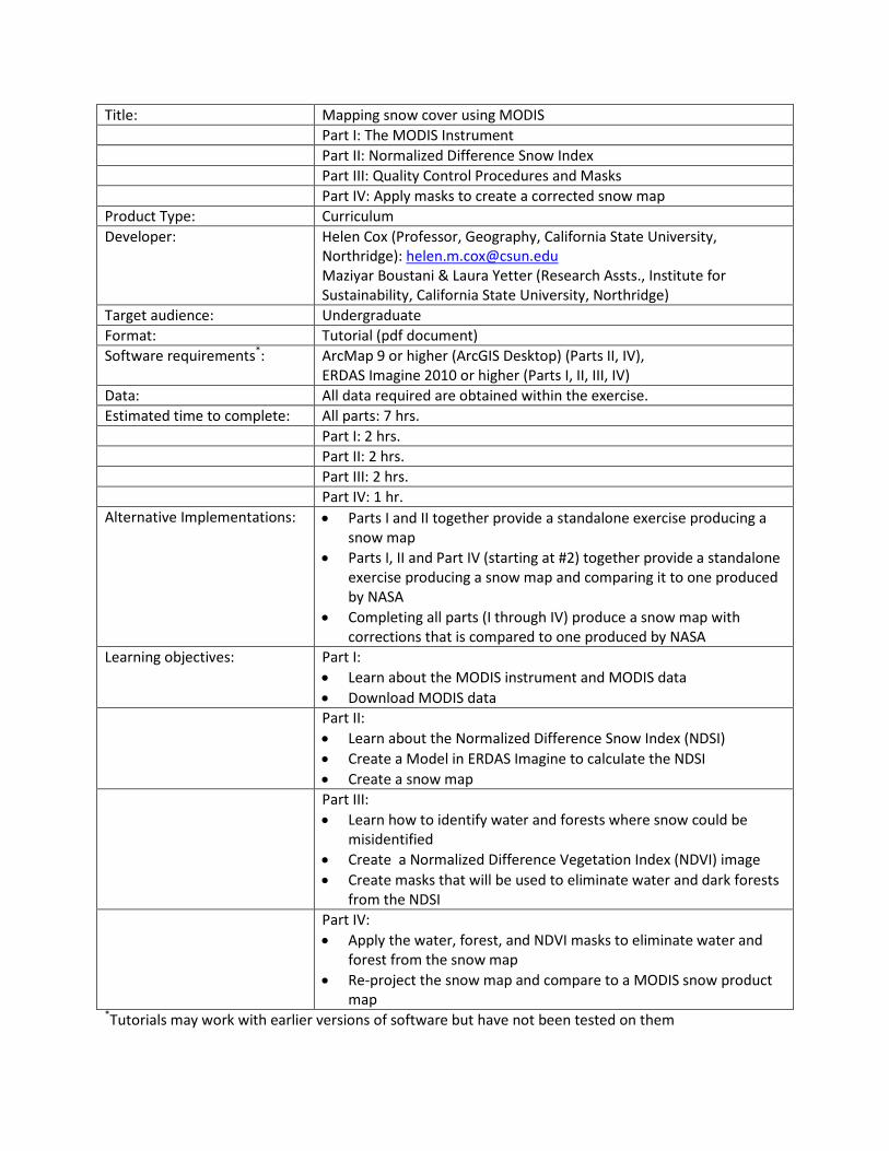
Title: Mapping snow cover using MODIS Part I: The MODIS Instrument Part II: Normalized Difference Snow Index Part III: Quality Control Procedures and Masks Part IV: Apply masks to create a corrected snow map Product Type: Curriculum Developer: Helen Cox (Professor, Geography, California State University,

Northridge): helen.m.cox@csun.edu Maziyar Boustani & Laura Yetter (Research Assts., Institute for Sustainability, California State University, Northridge)

Target audience: Undergraduate Format: Tutorial (pdf document) Software requirements*: ArcMap 9 or higher (ArcGIS Desktop) (Parts II, IV),

ERDAS Imagine 2010 or higher (Parts I, II, III, IV) Data: All data required are obtained within the exercise. Estimated time to complete: All parts: 7 hrs. Part I: 2 hrs. Part II: 2 hrs. Part III: 2 hrs. Part IV: 1 hr. Alternative Implementations: • Parts I and II together provide a standalone exercise producing a

snow map • Parts I, II and Part IV (starting at #2) together provide a standalone

exercise producing a snow map and comparing it to one produced by NASA

• Completing all parts (I through IV) produce a snow map with corrections that is compared to one produced by NASA

Learning objectives: Part I: • Learn about the MODIS instrument and MODIS data • Download MODIS data

Part II: • Learn about the Normalized Difference Snow Index (NDSI) • Create a Model in ERDAS Imagine to calculate the NDSI • Create a snow map

Part III: • Learn how to identify water and forests where snow could be

misidentified • Create a Normalized Difference Vegetation Index (NDVI) image • Create masks that will be used to eliminate water and dark forests

from the NDSI Part IV:

• Apply the water, forest, and NDVI masks to eliminate water and forest from the snow map

• Re-project the snow map and compare to a MODIS snow product map

*Tutorials may work with earlier versions of software but have not been tested on them

Mapping snow cover using MODIS

Part II: Normalized Difference Snow Index

Objectives

Learn about the Normalized Difference Snow Index (NDSI)

Create a Model in ERDAS Imagine to calculate the NDSI

Create a snow map

NDSI

Information on snow cover is important for a variety of reasons (estimates of freshwater storage,

indicator of global change, climate modeling and feedback effects). Trying to identify snow cover only

using the visible reflected light may be difficult because many things appear white such as clouds, sand,

surf, salt beds or even rocks. MODIS is used to monitor snow cover from space using the Normalize

Difference Snow Index (NDSI), with some corrections added for special circumstances. The NDSI uses

visible and short wave near infrared bands to identify snow.

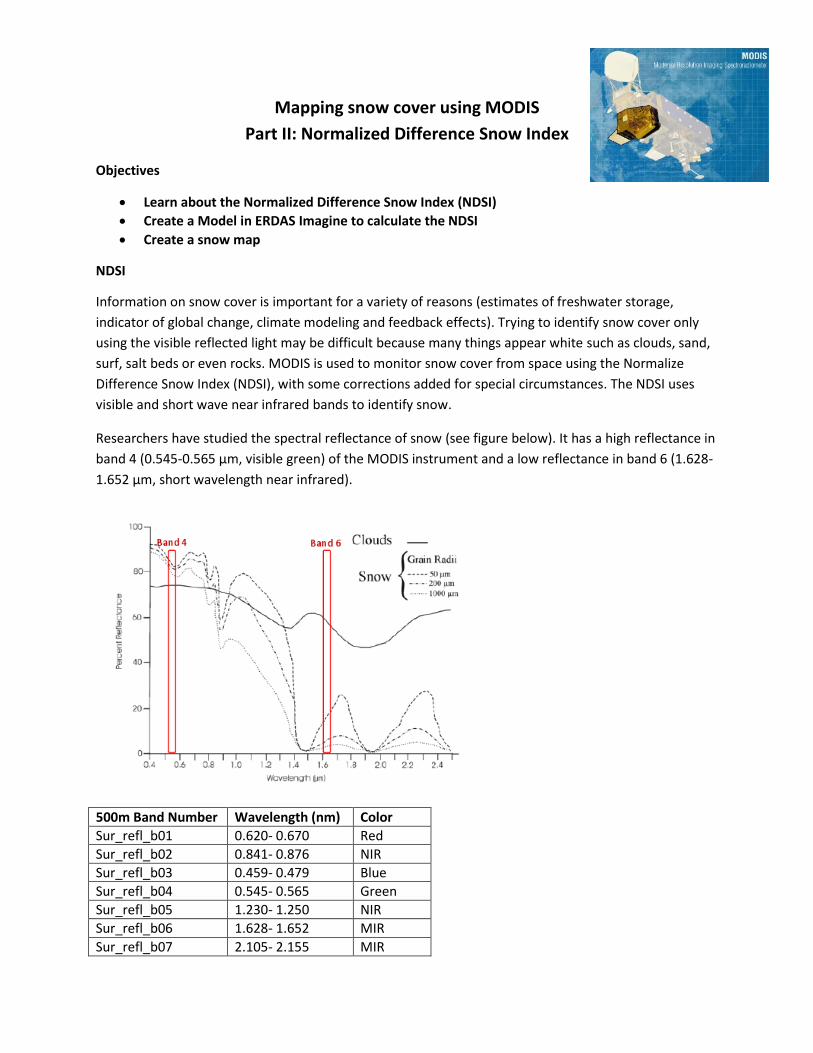
Researchers have studied the spectral reflectance of snow (see figure below). It has a high reflectance in

band 4 (0.545-0.565 µm, visible green) of the MODIS instrument and a low reflectance in band 6 (1.628-

1.652 µm, short wavelength near infrared).

500m Band Number Wavelength (nm) Color

Sur_refl_b01 0.620- 0.670 Red

Sur_refl_b02 0.841- 0.876 NIR

Sur_refl_b03 0.459- 0.479 Blue

Sur_refl_b04 0.545- 0.565 Green

Sur_refl_b05 1.230- 1.250 NIR

Sur_refl_b06 1.628- 1.652 MIR

Sur_refl_b07 2.105- 2.155 MIR

The NDSI is a normalized ratio of the difference in reflectance in these bands that takes advantage of the

unique signature and spectral differences to identify snow from surrounding features even clouds. The

equation for the NDSI is

NDSI= (band 4 – band 6)/( band 4 + band 6)

NDSI is calculated on a pixel-by-pixel basis and will generate a gray scale image with high values (bright

pixels) representing snow. The NDSI not only distinguishes snow versus non snow covered areas and

clouds, but also reduces the influence of atmospheric effects in the readings. The MODIS algorithm sets

a threshold value of 0.4 for snow (i.e. if NDSI > 0.4 pixel is snow, else not snow).

There are some nuances, however, with distinguishing snow from other non snow features such as

water or dense forests because they have similar NDSI readings to snow. These features have low

reflectance (they are good absorbers) and cause the NDSI denominator to be small. Then only small

increases in band 4 are enough to increase the NDSI value and misclassify a pixel as snow (Hall et al

2002). Therefore in addition to the NDSI it is necessary to examine reflectance at other wavelengths to

distinguish these features from snow cover.

To separate water bodies from snow, a pixel should be mapped as water if the reflectance in band 2

(0.841- 0.876 µm) is less than 11% even if the NDSI is greater than or equal to 0.4. To identify dark

forested areas, if the NDSI is greater than or equal to 0.4 (snow) but the reflectance in band 4 (0.545 -

0.565 µm) is less than 10% a pixel will be marked as forest. If a pixel NDSI value is less than 0.4 (not

snow) but the NDVI is approximately 0.1 the pixel could be snow-covered forest (Hall et al 2002). These

measures prevent low reflective features like water bodies and dense forest canopies from being

misclassified as snow. These corrections will be addressed in future exercises.

NDSI Model

In this exercise we will build a model in ERDAS Imagine to calculate NDSI from the MODIS image we

downloaded in the last exercise. Note that the pixel values in the reflectance image are whole numbers

with a range from -100 to 16000 and pixels of no data have a value of -28672. In order to calculate NDSI

they need to be scaled by a factor of 0.0001. See documentation at:

https://lpdaac.usgs.gov/products/modis_products_table/myd09gq

Open Imagine and open your .img MODIS image (To produce a true color image again change the band combination as necessary using the Table above).

Open the spatial modeler, select Modeler button from Imagine’s main menu bar. (Or in ERDAS 2010>

Toolbox Tab > Model Maker).

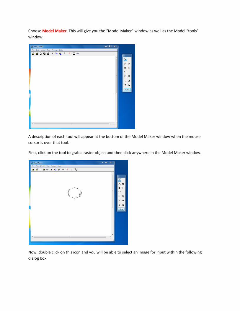
Choose Model Maker. This will give you the “Model Maker” window as well as the Model “tools”

window:

A description of each tool will appear at the bottom of the Model Maker window when the mouse

cursor is over that tool.

First, click on the tool to grab a raster object and then click anywhere in the Model Maker window.

Now, double click on this icon and you will be able to select an image for input within the following

dialog box:

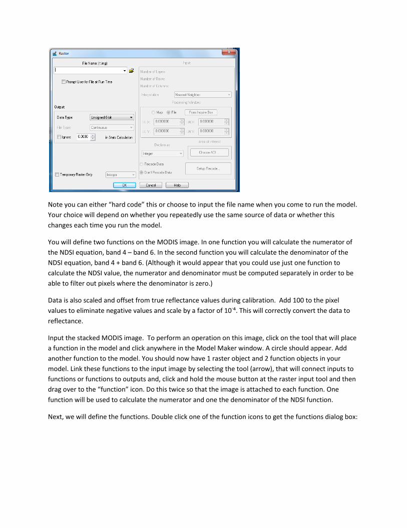
Note you can either “hard code” this or choose to input the file name when you come to run the model.

Your choice will depend on whether you repeatedly use the same source of data or whether this

changes each time you run the model.

You will define two functions on the MODIS image. In one function you will calculate the numerator of

the NDSI equation, band 4 – band 6. In the second function you will calculate the denominator of the

NDSI equation, band 4 + band 6. (Although it would appear that you could use just one function to

calculate the NDSI value, the numerator and denominator must be computed separately in order to be

able to filter out pixels where the denominator is zero.)

Data is also scaled and offset from true reflectance values during calibration. Add 100 to the pixel

values to eliminate negative values and scale by a factor of 10-⁴. This will correctly convert the data to

reflectance.

Input the stacked MODIS image. To perform an operation on this image, click on the tool that will place

a function in the model and click anywhere in the Model Maker window. A circle should appear. Add

another function to the model. You should now have 1 raster object and 2 function objects in your

model. Link these functions to the input image by selecting the tool (arrow), that will connect inputs to

functions or functions to outputs and, click and hold the mouse button at the raster input tool and then

drag over to the “function” icon. Do this twice so that the image is attached to each function. One

function will be used to calculate the numerator and one the denominator of the NDSI function.

Next, we will define the functions. Double click one of the function icons to get the functions dialog box:

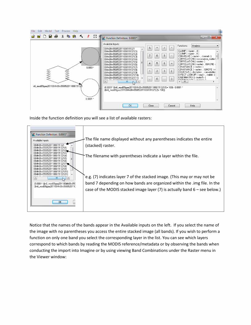
Inside the function definition you will see a list of available rasters:

The file name displayed without any parentheses indicates the entire

(stacked) raster.

The filename with parentheses indicate a layer within the file.

e.g. (7) indicates layer 7 of the stacked image. (This may or may not be

band 7 depending on how bands are organized within the .img file. In the

case of the MODIS stacked image layer (7) is actually band 6 – see below.)

Notice that the names of the bands appear in the Available inputs on the left. If you select the name of

the image with no parentheses you access the entire stacked image (all bands). If you wish to perform a

function on only one band you select the corresponding layer in the list. You can see which layers

correspond to which bands by reading the MODIS reference/metadata or by observing the bands when

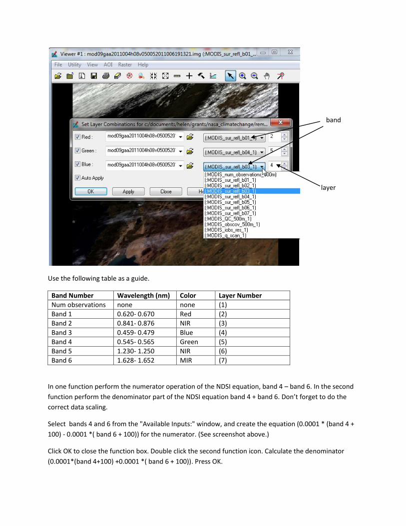
conducting the import into Imagine or by using viewing Band Combinations under the Raster menu in

the Viewer window:

band

layer

Use the following table as a guide.

Band Number Wavelength (nm) Color Layer Number

Num observations none none (1)

Band 1 0.620- 0.670 Red (2)

Band 2 0.841- 0.876 NIR (3)

Band 3 0.459- 0.479 Blue (4)

Band 4 0.545- 0.565 Green (5)

Band 5 1.230- 1.250 NIR (6)

Band 6 1.628- 1.652 MIR (7)

In one function perform the numerator operation of the NDSI equation, band 4 – band 6. In the second

function perform the denominator part of the NDSI equation band 4 + band 6. Don’t forget to do the

correct data scaling.

Select bands 4 and 6 from the "Available Inputs:" window, and create the equation (0.0001 * (band 4 +

100) - 0.0001 *( band 6 + 100)) for the numerator. (See screenshot above.)

Click OK to close the function box. Double click the second function icon. Calculate the denominator

(0.0001*(band 4+100) +0.0001 *( band 6 + 100)). Press OK.

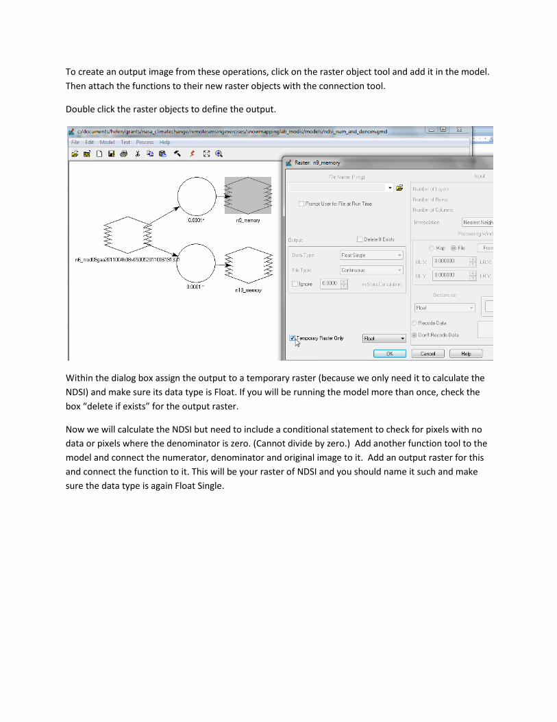
To create an output image from these operations, click on the raster object tool and add it in the model.

Then attach the functions to their new raster objects with the connection tool.

Double click the raster objects to define the output.

Within the dialog box assign the output to a temporary raster (because we only need it to calculate the

NDSI) and make sure its data type is Float. If you will be running the model more than once, check the

box “delete if exists” for the output raster.

Now we will calculate the NDSI but need to include a conditional statement to check for pixels with no

data or pixels where the denominator is zero. (Cannot divide by zero.) Add another function tool to the

model and connect the numerator, denominator and original image to it. Add an output raster for this

and connect the function to it. This will be your raster of NDSI and you should name it such and make

sure the data type is again Float Single.

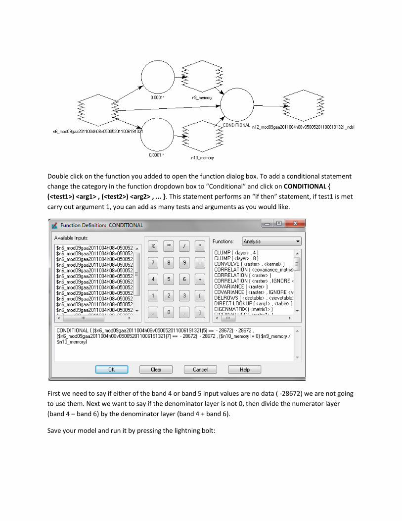
Double click on the function you added to open the function dialog box. To add a conditional statement

change the category in the function dropdown box to “Conditional” and click on CONDITIONAL {

(<test1>) <arg1> , (<test2>) <arg2> , ... }. This statement performs an “if then” statement, if test1 is met

carry out argument 1, you can add as many tests and arguments as you would like.

First we need to say if either of the band 4 or band 5 input values are no data ( -28672) we are not going

to use them. Next we want to say if the denominator layer is not 0, then divide the numerator layer

(band 4 – band 6) by the denominator layer (band 4 + band 6).

Save your model and run it by pressing the lightning bolt:

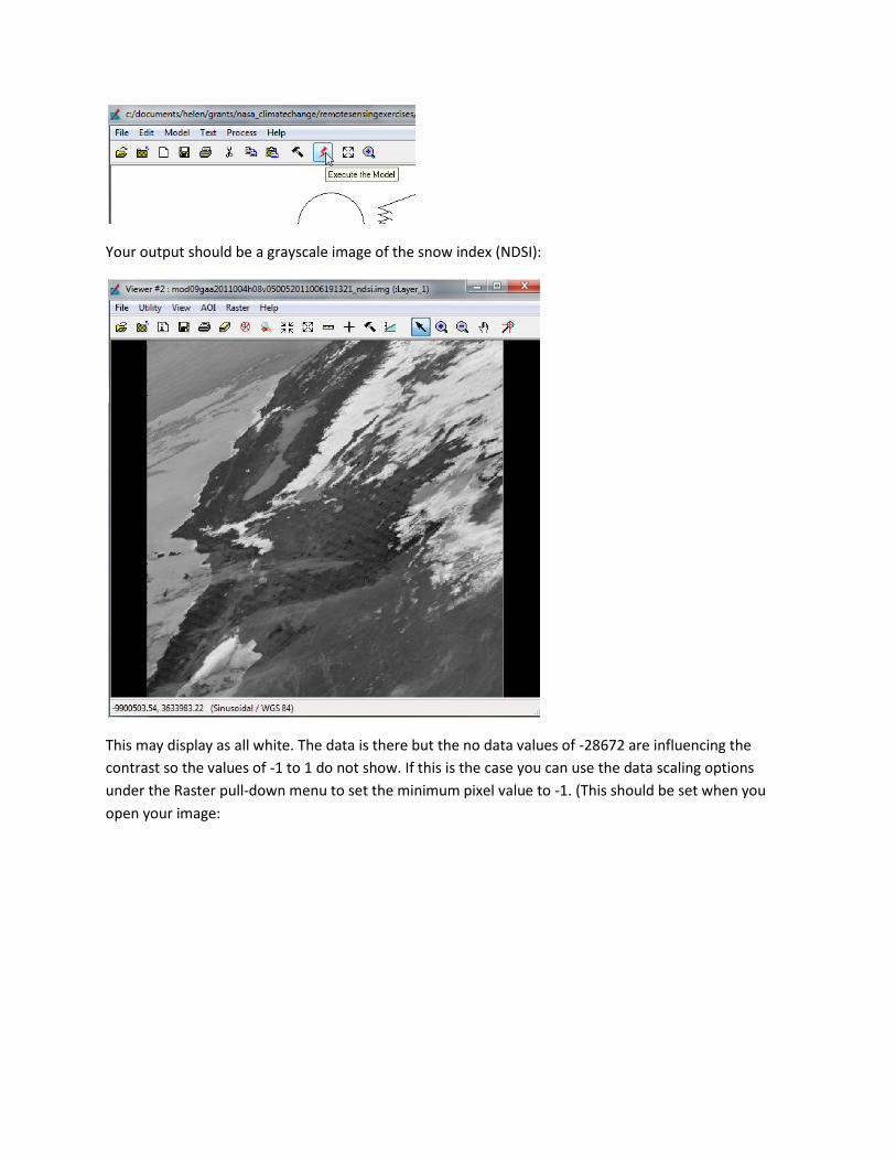
Your output should be a grayscale image of the snow index (NDSI):

This may display as all white. The data is there but the no data values of -28672 are influencing the

contrast so the values of -1 to 1 do not show. If this is the case you can use the data scaling options

under the Raster pull-down menu to set the minimum pixel value to -1. (This should be set when you

open your image:

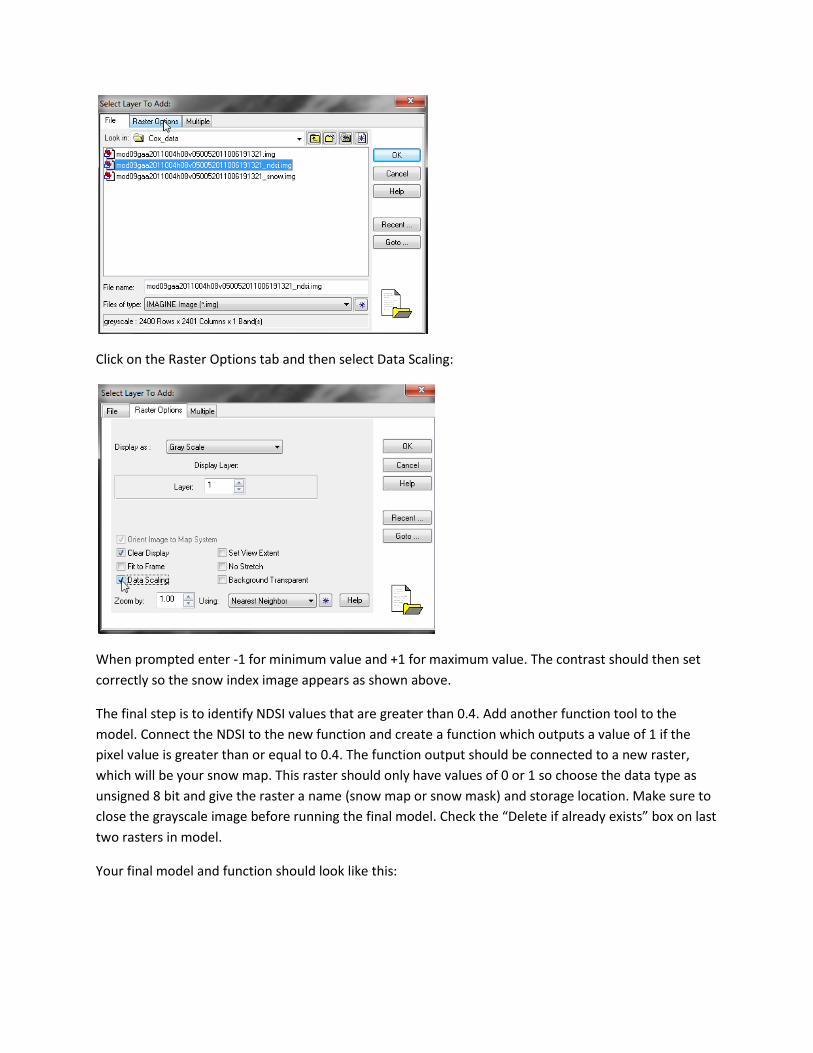
Click on the Raster Options tab and then select Data Scaling:

When prompted enter -1 for minimum value and +1 for maximum value. The contrast should then set

correctly so the snow index image appears as shown above.

The final step is to identify NDSI values that are greater than 0.4. Add another function tool to the

model. Connect the NDSI to the new function and create a function which outputs a value of 1 if the

pixel value is greater than or equal to 0.4. The function output should be connected to a new raster,

which will be your snow map. This raster should only have values of 0 or 1 so choose the data type as

unsigned 8 bit and give the raster a name (snow map or snow mask) and storage location. Make sure to

close the grayscale image before running the final model. Check the “Delete if already exists” box on last

two rasters in model.

Your final model and function should look like this:

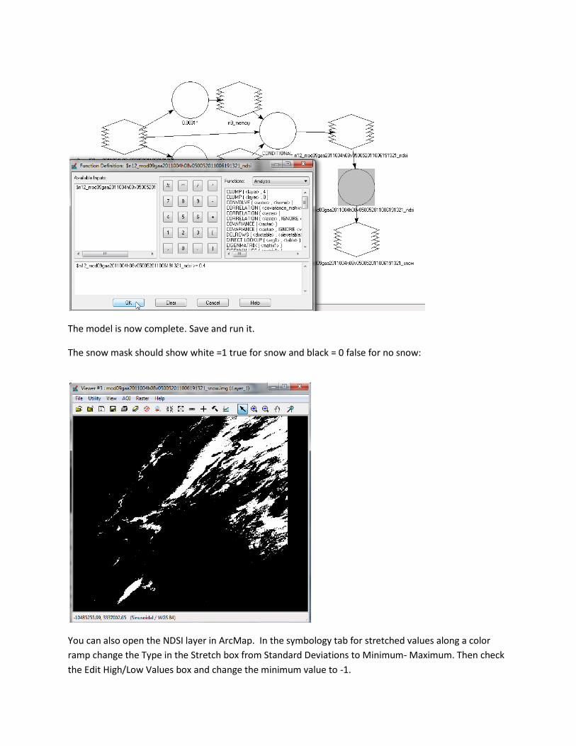
The model is now complete. Save and run it.

The snow mask should show white =1 true for snow and black = 0 false for no snow:

You can also open the NDSI layer in ArcMap. In the symbology tab for stretched values along a color

ramp change the Type in the Stretch box from Standard Deviations to Minimum- Maximum. Then check

the Edit High/Low Values box and change the minimum value to -1.

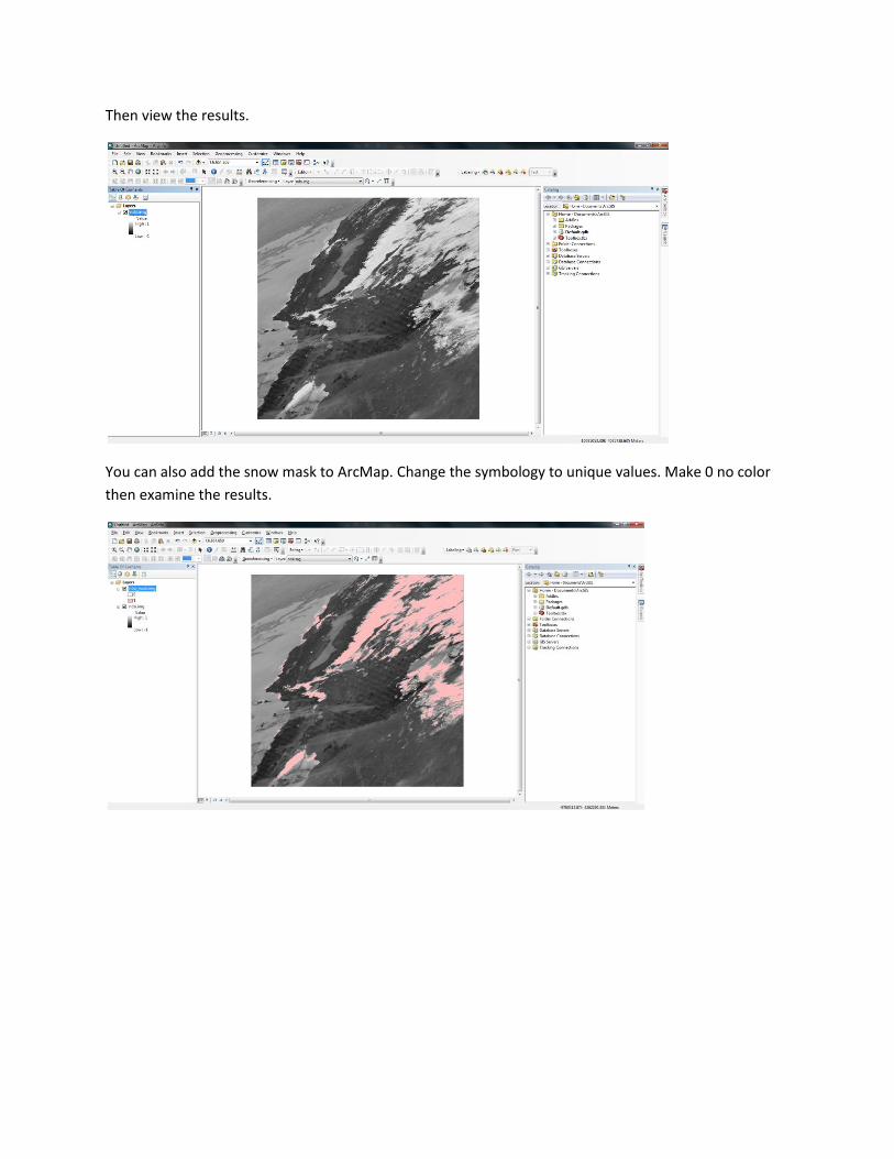
Then view the results.

You can also add the snow mask to ArcMap. Change the symbology to unique values. Make 0 no color

then examine the results.