modified power series solutions and the basic method of frobeniushowellkb.uah.edu/de2/lecture...
TRANSCRIPT

33
Modified Power Series Solutions and theBasic Method of Frobenius
The partial sums of a power series solution about an ordinary point x0 of a differential equation
provide fairly accurate approximations to the equation’s solutions at any point x near x0 . This
is true even if relatively low-order partial sums are used (provided you are just interested in the
solutions at points very near x0 ). However, these power series typically converge slower and
slower as x moves away from x0 towards a singular point, with more and more terms then being
needed to obtain reasonably accurate partial sum approximations. As a result, the power series
solutions derived in the previous two chapters usually tell us very little about the solutions near
singular points. This is unfortunate because, in some applications, the behavior of the solutions
near certain singular points can be a rather important issue.
Fortunately, in many of those applications, the singular point in question is not that “bad”
a singular point, and a modification of the algebraic method discussed in the previous chapters
can be used to obtain “modified” power series solutions about these points. That is what we will
develop in this and the next two chapters.
By the way, we will only consider second-order homogeneous linear differential equations.
One can extend the discussion here to first- and higher-order equations, but the important examples
are all second-order.
33.1 Euler Equations and Their Solutions
The simplest examples of the sort of equations of interest in this chapter are those discussed back
in chapter 19, the Euler equations. Let us quickly review them and take a look at what happens
to their solutions about their singular points.
Recall that a standard second-order Euler equation is a differential equation that can be
written as
α0x2 y′′ + β0xy′ + γ0 y = 0
where α0 , β0 and γ0 are real constants with α0 6= 0 . Recall, also, that the basic method for
solving such an equation begins with attempting a solution of the form y = xr where r is a
2/5/2014
Chapter & Page: 33–2 Modified Power Series Solutions and the Basic Method of Frobenius
constant to be determined. Plugging y = xr into the differential equation, we get
α0x2[
xr]′′ + β0x
[
xr]′ + γ0
[
xr]
= 0
→֒ α0x2[
r(r − 1)xr−2]
+ β0x[
r xr−1]
+ γ0
[
xr]
= 0
→֒ xr[
α0r(r − 1) + β0r + γ0
]
= 0
→֒ α0r(r − 1) + β0r + γ0 = 0 .
The last equation above is the indicial equation, which we typically rewrite as
α0r 2 + (β0 − α0)r + γ0 = 0 ,
and, from which, we can easily determine the possible values of r using basic algebra.
Generalizing slightly, we have the shifted Euler equation
α0(x − x0)2 y′′ + β0(x − x0)y′ + γ0 y = 0
where x0 , α0 , β0 and γ0 are real constants with α0 6= 0 . Notice that x0 is the one and only
singular point of this equation. (Notice, also, that a standard Euler equation is a shifted Euler
equation with x0 = 0 .)
To solve this slight generalization of a standard Euler equation, use the obvious slight
generalization of the basic method for solving a standard Euler equation: First set
y = (x − x0)r ,
where r is a yet unknown constant. Then plug this into the differential equation, compute, and
simplify. Unsurprisingly, you end up with the corresponding indicial equation
α0r(r − 1) + β0r + γ0 = 0 ,
which you can rewrite as
α0r 2 + (β0 − α0)r + γ0 = 0 ,
and then solve for r , just as with the standard Euler equation. And, as with a standard Euler
equation, there are then only three basic possibilities regarding the roots r1 and r2 to the indicial
equation and the corresponding solutions to the Euler equations:
1. The two roots can be two different real numbers, r1 6= r2 .
In this case, the general solution to the differential equation is
y(x) = c1 y1(x) + c2 y2(x)
with, at least when x > x0 ,1
y1(x) = (x − x0)r1 and y2(x) = (x − x0)
r2 .
1 In all of these cases, the formulas and observations also hold when x < x0 , though we may wish to replace x − x0
with |x − x0| to avoid minor issues with (x − x0)r for certain values of r (such as r = 1/2 ).

Euler Equations and Their Solutions Chapter & Page: 33–3
Observe that, for j = 1 or j = 2 ,
limx→x+
0
∣∣y j(x)
∣∣ = lim
x→x0
|x − x0|r j =
0 if r j > 0
1 if r j = 0
+∞ if r j < 0
.
2. The two roots can be the same real number, r2 = r1 .
In this case, we can use reduction of order and find that the general solution to the
differential equation is (when x > x0 )
y(x) = c1 y1(x) + c2 y2(x)
with
y1(x) = (x − x0)r1 and y2(x) = (x − x0)
r1 ln |x − x0| .
After recalling how ln |X | behaves when X ≈ 0 (with X = x − x0 ), we see that
limx→x+
0
|y2(x)| = limx→x0
∣∣(x − x0)
r1 ln |x − x0|∣∣ =
{
0 if ri > 0
+∞ if ri ≤ 0.
3. Finally, the two roots can be complex conjugates of each other
r1 = λ + iω and r2 = λ − iω with ω > 0 .
After recalling that
Xλ±iω = Xλ [cos(ω ln |X |) ± i sin(ω ln |X |)] for X > 0
(see the discussion of complex exponents in section 19.2),we find that the general solution
to the differential equation for x > x0 can be given by
y(x) = c1 y1(x) + c2 y2(x)
where y1 and y2 are the real-valued functions
y1(x) = (x − x0)λ cos(ω ln |x − x0|)
and
y2(x) = (x − x0)λ sin(ω ln |x − x0|) .
The behavior of these solutions as x → x0 is a bit more complicated. First observe that,
as X goes from 1 to 0 , ln |X | goes from 0 to −∞ , which means that sin(ω ln |X |)and cos(ω ln |X |) then must oscillate infinitely many times between their maximum and
minimum values of 1 and −1 , as illustrated in figure 33.1a. So sin(ω ln |X |) and
cos(ω ln |X |) are bounded, but do not approach any single value as X → 0 . Taking into
account how Xλ behaves (and replacing X with x − x0 ), we see that
limx→x+
0
|yi(x)| = 0 if λ > 0 ,
and
limx→x+
0
|yi (x)| does not exist if λ ≤ 0 .

Chapter & Page: 33–4 Modified Power Series Solutions and the Basic Method of Frobenius
(a) (b)
11
11
−1−1
XX
Figure 33.1: Graphs of (a) sin(ω ln |X |) , and (b) Xλ sin(ω ln |X |) (with ω = 10 and
λ = 11/10 ).
Notice that the behavior of these solutions as x → x0 depends strongly on the values of r1
and r2 . Notice, also, that you can rarely arbitrarily assign the initial values y(x0) and y′(x0)
for these solutions.
!◮Example 33.1: Consider the shifted Euler equation
(x − 3)2 y′′ − 2y = 0 .
If y = (x − 3)r for any constant r , then
(x − 3)2 y′′ − 2y = 0
→֒ (x − 3)2[
(x − 3)r]′′ − 2
[
(x − 3)r]
= 0
→֒ (x − 3)2r(r − 1)(x − 3)r−2 − 2(x − 3)r = 0
→֒ (x − 3)r [r(r − 1) − 2] = 0 .
Thus, for y = (x −3)r to be a solution to our differential equation, r must satisfy the indicial
equation
r(r − 1) − 2 = 0 .
After rewriting this as
r 2 − r − 2 = 0 ,
and factoring,
(r − 2)(r + 1) = 0 ,
we see that the two solutions to the indicial equation are r = 2 and r = −1 . Thus, the
general solution to our differential equation is
y = c1(x − 3)2 + c2(x − 3)−1 .
This has one term that vanishes as x → 3 and another that blows up as x → 3 . In particular,
we cannot insist that y(3) be any particular nonzero number, say, “ y(3) = 2 ”.

Euler Equations and Their Solutions Chapter & Page: 33–5
!◮Example 33.2: Now consider
x2 y′′ + xy′ + y = 0 ,
which is a shifted Euler equation, but with “shift” x0 = 0 .
The indicial equation for this is
r(r − 1) + r + 1 = 0 ,
which simplifies to
r 2 + 1 = 0 .
So,
r = ±√
−1 = ±i .
In other words, r = λ ± iω with λ = 0 and ω = 1 . Consequently, the general solution to
the differential equation in this example is given by
y = c1x0 cos(1 ln |x |) + c2x0 sin(1 ln |x |) .
which we naturally would prefer to write more simply as
y = c1 cos(ln |x |) + c2 sin(ln |x |) .
Here, neither term vanishes or blows up. Instead, as x goes from 1 to 0 , we have ln |x |going from 0 to −∞ . This means that the sine and cosine terms here oscillate infinitely
many times as x goes from 1 to 0 , similar to the function illustrated in figure 33.1a. Again,
there is no way we can require that “ y(0) = 2 ”.
The “blowing up” or “vanishing” of solutions illustrated above is typical behavior of solutions
about the singular points of their differential equations. Sometimes it is important to know just
how the solutions to a differential equation behave near a singular point x0 . For example, if you
know a solution describes some process that does not blow up as x → x0 , then you know that
those solutions that do blow up are irrelevant to your problem (this will become very important
when we study boundary-value problems).
The tools we will develop in this chapter will yield “modified power series solutions” around
singular points for at least some differential equations. The behavior of the solutions near these
singular points can then be deduced from these modified power series. For which equations will
this analysis be appropriate? Before answering that, I must first tell you the difference between
a “regular” and an “irregular” singular point.
Chapter & Page: 33–6 Modified Power Series Solutions and the Basic Method of Frobenius
33.2 Regular and Irregular Singular Points (and theFrobenius Radius of Convergence)
Basic Terminology
Assume x0 is singular point on the real line for some given homogeneous linear second-order
differential equation
ay′′ + by′ + cy = 0 . (33.1)
We will say that x0 is a regular singular point for this differential equation if and only if that
differential equation can be rewritten as
(x − x0)2α(x)y′′ + (x − x0)β(x)y′ + γ (x)y = 0 (33.2)
where α , β and γ are ‘suitable, well-behaved’ functions about x0 with α(x0) 6= 0 . The
above form will be called a quasi-Euler form about x0 for the given differential equation, and
the shifted Euler equation
(x − x0)2α0 y′′ + (x − x0)β0 y′ + γ0 y = 0 (33.3a)
where
α0 = α(x0) , β0 = β(x0) and γ0 = γ (x0) . (33.3b)
will be called the associated (shifted) Euler equation (about x0 ).
Precisely what we mean above by “ ‘suitable, well-behaved’ functions about x0 ” depends,
in practice, on the coefficients of the original differential equation. In general, it means that the
functions α , β and γ in equation (33.2) are all analytic at x0 . However, if the coefficients of
the original equation (the a , b and c in equation (33.1)) are rational functions, then we will be
able to further insist that the α , β and γ in the quasi-Euler form be polynomials.
It is quite possible that our differential equation cannot be written in quasi-Euler form about
x0 . Then we will say x0 is an irregular singular point for our differential equation. Thus,
every singular point on the real line for our differential equation is classified as being regular
or irregular depending on whether the differential equation can be rewritten in quasi-Euler form
about that singular point.
While we are at it, let’s also define the Frobenious radius of analyticity about any point z0
for our differential equation: It is simply the distance between z0 and the closest singular point
zs other than z0 , provided such a point exists. If no such zs exists, then the Frobenius radius of
analyticity is ∞ . The Frobenius radius of analyticity will play almost the same role as played
by the radius of analyticity in the previous two chapters. In fact, it is the radius of analyticity if
z0 happens to be an ordinary point.
!◮Example 33.3 (Bessel Equations): Let ν be any positive real constant. Bessel’s equation
of order ν is the differential equation 2
y′′ + 1
xy′ +
[
1 −(
ν
x
)2]
y = 0 .
The coefficients of this,
a(x) = 1 , b(x) = 1
xand c(x) = 1 −
(ν
x
)2
= x2 − ν2
x2,
2 Bessel’s equations and their solutions often arise in two-dimensional problems involving circular objects.
Regular and Irregular Singular Points Chapter & Page: 33–7
are rational functions. Multiplying through by x2 then gives us
x2 y′′ + xy′ +[
x2 − ν2]
y = 0 . (33.4)
Clearly, x0 = 0 is the one and only singular point for this differential equation. This, in
turn, means that the Frobenius radius of analyticity about x0 = 0 is ∞ (though the radius of
analyticity, as defined in chapter 31, is 0 since x0 = 0 is a singular point.)
Now observe that the last differential equation is
(x − 0)2α(x)y′′ + (x − 0)β(x)y′ + γ (x)y = 0 . (33.5a)
where α , β and γ are the simple polynomials
α(x) = 1 , β(x) = 1 and γ (x) = x2 − ν2 , (33.5b)
which are certainly analytic about x0 = 0 (and every other point on the complex plane).
Moreover, since
α(0) = 1 6= 0 , β(0) = 1 and γ (0) = −ν2 ,
we now have that:
1. The Bessel equation of order ν can be written in quasi-Euler form about x0 = 0 .
2. The singular point x0 = 0 is a regular singular point.
and
3. The associated Euler equation about x0 = 0 is
(x − 0)2 · 1y′′ + (x − 0) · 1y′ − ν2 y = 0 ,
which, of course, is normally written
x2 y′′ + xy′ − ν2 y = 0 .
Two quick notes before going on:
1. Often, the point of interest is x0 = 0 , in which case we will write equation (33.2) more
simply as
x2α(x)y′′ + xβ(x)y′ + γ (x)y = 0 (33.6)
with the associated Euler equation being
x2α0 y′′ + xβ0 y′ + γ0 y = 0 (33.7a)
where
α0 = α(0) , β0 = β(0) and γ0 = γ (0) . (33.7b)
2. In fact, any singular point on the complex plane can be classified as regular or irregular.
However, this won’t be particularly relevant to us. Our interest will only be in whether
given singular points on the real line are regular or not.

Chapter & Page: 33–8 Modified Power Series Solutions and the Basic Method of Frobenius
Testing for Regularity
As illustrated in our last example, if the coefficients in our original differential equation are
relatively simple rational functions, then it can be relatively straightforward to show that a given
singular point x0 is or is not regular by seeing if we can or cannot rewrite the equation in quasi-
Euler form about x0 . An advantage of deriving this quasi-Euler form (if possible) is that we
will want this quasi-Euler form in solving our differential equation. However, there are possible
difficulties. If we cannot rewrite our equation in quasi-Euler form, then we may be left with the
question of whether x0 truly is an irregular singular point, or whether we just weren’t clever
enough to get the equation into quasi-Euler form. Also, if the coefficients in our original equation
are not so simple, then the process of attempting to convert it to quasi-Euler form may be quite
challenging.
A useful test for regularity is easily derived by first assuming that x0 is a regular singular
point for
a(x)y′′ + b(x)y′ + c(x)y = 0 . (33.8)
By definition, this means that this differential equation can be rewritten as
(x − x0)2α(x)y′′ + (x − x0)β(x)y′ + γ (x)y = 0 (33.9)
where α , β and γ are functions analytic at x0 with α(x0) 6= 0 . Dividing each of these two
equations by its first coefficient converts our differential equation, respectively, to the two forms
y′′ + b(x)
a(x)y′ + c(x)
a(x)y = 0
and
y′′ + β(x)
(x − x0)α(x)y′ + γ (x)
(x − x0)2α(x)y = 0 .
But these last two equations describe the same differential equation, and have the same first
coefficients. Clearly, the other coefficients must also be the same, giving us
b(x)
a(x)= β(x)
(x − x0)α(x)and
c(x)
a(x)= γ (x)
(x − x0)2α(x).
Equivalently,
(x − x0)b(x)
a(x)= β(x)
α(x)and (x − x0)
2 c(x)
a(x)= γ (x)
α(x).
From this and the fact that α , β and γ are analytic at x0 with α(x0) 6= 0 we get that the two
limits
limx→x0
(x − x0)b(x)
a(x)= lim
x→x0
β(x)
α(x)= β(x0)
α(x0)
and
limx→x0
(x − x0)2 c(x)
a(x)= lim
x→x0
γ (x)
α(x)= γ (x0)
α(x0)
are finite.
So, x0 being a regular singular point assures us that the above limits are finite. Consequently,
if those limits are not finite, then x0 cannot be a regular singular point for our differential equation.
That gives us

Regular and Irregular Singular Points Chapter & Page: 33–9
Lemma 33.1 (test for irregularity)
Assume x0 is a singular point on the real line for
a(x)y′′ + b(x)y′ + c(x)y = 0 .
If either of the two limits
limx→x0
(x − x0)b(x)
a(x)and lim
x→x0
(x − x0)2 c(x)
a(x)
is not finite, then x0 is an irregular singular point for the differential equation.
This lemma is just a test for irregularity. It can be expanded to a more complete test if we
make mild restrictions on the coefficients of the original differential equation. In particular, using
properties of polynomials and rational functions, we can verify the following:
Theorem 33.2 (testing for regular singular points (ver.1))
Assume x0 is a singular point on the real line for
a(x)y′′ + b(x)y′ + c(x)y = 0
where a , b and c are rational functions. Then x0 is a regular singular point for this differential
equation if and only if the two limits
limx→x0
(x − x0)b(x)
a(x)and lim
x→x0
(x − x0)2 c(x)
a(x)
are both finite values. Moreover, if x0 is a regular singular point for the differential equation,
then this differential equation can be written in quasi-Euler form
(x − x0)2α(x)y′′ + (x − x0)β(x)y′ + γ (x)y = 0
where α , β and γ are polynomials with α(x0) 6= 0 .
The full proof of this (along with a similar theorem applicable when the coefficients are
merely quotients of analytic functions) is discussed in an appendix, section 33.7.
!◮Example 33.4: Consider the differential equation
y′′ + 1
x2y′ +
[
1 − 1
x2
]
y = 0 .
Clearly, x0 = 0 is a singular point for this equation. Writing out the limits given in the above
theorem (with x0 = 0 ) yields
limx→0
(x − 0)b(x)
a(x)= lim
x→x · x−2
1= lim
x→0
1
x
and
limx→0
(x − 0)2 c(x)
a(x)= lim
x→x2 · 1 − x−2
1= lim
x→0
[
x2 − 1]
,
The first limit is certainly not finite. So our test for regularity tells us that x0 = 0 is an
irregular singular point for this differential equation.
Chapter & Page: 33–10 Modified Power Series Solutions and the Basic Method of Frobenius
!◮Example 33.5: Consider
2xy′′ − 4y′ − y = 0 .
Again, x0 = 0 is clearly the only singular point. Now,
limx→0
(x − 0)b(x)
a(x)= lim
x→0x · −4
2x= −2
and
limx→0
(x − 0)2 c(x)
a(x)= lim
x→0x2 · −1
2x= 0 ,
both of which are finite. So x0 = 0 is a regular singular point for our equation, and it can be
written in quasi-Euler form about 0 . In fact, that form is obtained by simply multiplying the
original differential equation by x ,
2x2 y′′ − 4xy′ − xy = 0 .
33.3 The (Basic) Method of FrobeniusMotivation and Preliminary Notes
Let’s suppose we have a second-order differential equation with x0 as a regular singular point.
Then, as we just discussed, this differential equation can be written as
(x − x0)2α(x)y′′ + (x − x0)β(x)y′ + γ (x)y = 0
where α , β and γ are analytic at x0 with α(x0) 6= 0 . By continuity, when x ≈ x0 , we have
α(x) ≈ α0 , β(x) ≈ β0 and γ (x) ≈ γ0
where
α0 = α(x0) , β0 = β(x0) and γ0 = γ (x0) .
It should then seem reasonable that any solution y = y(x) to
(x − x0)2α(x)y′′ + (x − x0)β(x)y′ + γ (x)y = 0
can be approximated, at least when x ≈ x0 , by a corresponding solution to the associated shifted
Euler equation
(x − x0)2α0 y′′ + (x − x0)β0 y′ + γ0 y = 0 .
And since some solutions to this shifted Euler equation are of the form a0(x − x0)r where a0
is an arbitrary constant and r is a solution to the corresponding indicial equation,
α0r(r − 1) + β0r + γ0 = 0 ,
it seems reasonable to expect at least some solutions to our original differential equation to be
approximated by this a0(x − x0)r ,
y(x) ≈ a0(x − x0)r at least when x ≈ x0 .
The (Basic) Method of Frobenius Chapter & Page: 33–11
Now, this is equivalent to saying
y(x)
(x − x0)r≈ a0 when x ≈ x0 ,
which is more precisely stated as
limx→x0
y(x)
(x − x0)r= a0 . (33.10)
At this point, there are a number of ways we might ‘guess’ at solutions satisfying the last
approximation. Let us try a trick similar to one we’ve used before: Let us assume y is the known
approximate solution (x − x0)r multiplied by some yet unknown function a(x) ,
y(x) = (x − x0)r a(x) .
To satisfy equation (33.10), we must have
a(x0) = limx→x0
a(x) = limx→x0
y(x)
(x − x0)r= a0 ,
telling us that a(x) is reasonably well-behaved near x0 , perhaps even analytic. Well, let’s hope
it is analytic, because that means we can express a(x) as a power series about x0 with the
arbitrary constant a0 as the constant term,
a(x) =∞
∑
k=0
ak(x − x0)k .
Then, with luck and skill, we might be able to use the methods developed in the previous chapters
to find the ak’s in terms of a0 .
That is the starting point for what follows: We will assume a solution of the form
y(x) = (x − x0)r
∞∑
k=0
ak(x − x0)k
where r and the ak’s are constants to be determined, with a0 being arbitrary. This will yield
the “modified power series” solutions alluded to in the title of this chapter.
In the next subsection, we will describe a series of steps, generally called the (basic) method
of Frobenius, for finding such solutions. You will discover that much of it is very similar to the
algebraic method for finding power series solutions in chapter 31.
But before we start that, let me mention a few things about this method:
1. We will see that the method of Frobenius always yields at least one solution of the form
y(x) = (x − x0)r
∞∑
k=0
ak(x − x0)k
where r is a solution to the appropriate indicial equation. If the indicial equation for the
corresponding Euler equation
(x − x0)2α0 y′′ + (x − x0)β0 y′ + γ0 y = 0
has two distinct solutions, then we will see that the method often, but not always, leads
to an independent pair of such solutions.
Chapter & Page: 33–12 Modified Power Series Solutions and the Basic Method of Frobenius
2. If, however, that indicial equation has only one solution r , then the fact that the corre-
sponding shifted Euler equation has a ‘second solution’ in the form
(x − x0)r ln |x − x0|
may lead you to suspect that a ‘second solution’ to our original equation is of the form
(x − x0)r ln |x − x0|
∞∑
k=0
ak(x − x0)k .
That turns out to be almost, but not quite, the case.
Just what can be done when the basic Frobenius method does not yield an independent pair of
solutions will be discussed in the next chapter.
The (Basic) Method of Frobenius
Suppose we wish to find the solutions about some regular singular point x0 to some second-order
homogeneous linear differential equation
a(x)y′′ + b(x)y′ + c(x)y = 0
with a(x) , b(x) , and c(x) being rational functions.3 In particular, let us seek solutions to
Bessel’s equation of order 1/2 ,
y′′ + 1
xy′ +
[
1 − 1
4x2
]
y = 0 (33.11)
near the regular singular point x0 = 0 .
As with the algebraic method for finding power series solutions, there are two preliminary
steps:
Pre-Step 1. If not already specified, choose the regular singular point x0 .
For our example, we choose x0 = 0 , which we know is the only regular
singular point from the discussion in the previous section.
Pre-Step 2. Get the differential equation into the form
(x − x0)2α(x)y′′ + (x − x0)β(x)y′ + γ (x)y = 0 (33.12)
where α , β and γ are polynomials, with α(x0) 6= 0 , and with no factors shared by all
three.4
3 The “Frobenius method” for the more general equations is developed in chapter 35.4 It will actually suffice to get the differential equation into the form
Ay′′ + By′ + Cy = 0
where A , B and C are polynomials, preferably with no factors shared by all three. Using form (33.12) will
slightly simplify bookkeeping at one point, and will be convenient for discussions later.

The (Basic) Method of Frobenius Chapter & Page: 33–13
To get the given differential equation into the form desired, we multiply equa-
tion (33.11) by 4x2 . That gives us the differential equation
4x2 y′′ + 4xy′ + [4x2 − 1]y = 0 . (33.13)
(Yes, we could have just multiplied by x2 , but getting rid of any fractions will
simplify computation.)
Now for the basic method of Frobenius:
Step 1. (a) Assume a solution of the form
y = y(x) = (x − x0)r
∞∑
k=0
ak(x − x0)k (33.14a)
with a0 being an arbitrary nonzero constant.5,6
(b) Simplify this formula for the following computations by bringing the (x − x0)r
factor into the summation,
y = y(x) =∞
∑
k=0
ak(x − x0)k+r . (33.14b)
Step 2. Compute the corresponding modified power series for y′ and y′′ from the assumed
series for y by differentiating “term-by-term”.7 This time, you cannot drop the “k = 0”
term in the summations because this term is not necessarily a constant.
Since we’ve already decided x0 = 0 , we assume
y = y(x) = xr
∞∑
k=0
ak xk =∞
∑
k=0
ak xk+r (33.15)
with a0 6= 0 . Differentiating this term-by-term, we see that
y′ = d
dx
∞∑
k=0
ak xk+r
=∞
∑
k=0
d
dx
[
ak xk+r]
=∞
∑
k=0
ak(k + r)xk+r−1
and
y′′ = d
dx
∞∑
k=0
ak(k + r)xk+r−1
=∞
∑
k=0
d
dx
[
ak(k + r)xk+r−1]
=∞
∑
k=0
ak(k + r)(k + r − 1)xk+r−2 .
5 Insisting that a0 6= 0 will be important in determining the possible values of r .6 This procedure is valid whether or not x − x0 is positive or negative. However, a few readers may have concerns
about (x − x0)r being imaginary if x < x0 and r is, say, 1/2 . If you are one of those readers, go ahead and
assume x > x0 for now, and later read the short discussion of solutions on intervals with x < x0 on page 33–23.7 If you have any qualms about “term-by-term” differentiation here, see exercise 33.6 at the end of the chapter.
Chapter & Page: 33–14 Modified Power Series Solutions and the Basic Method of Frobenius
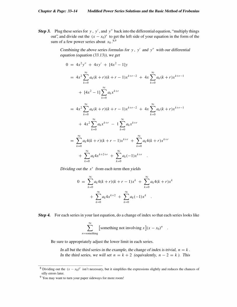
Step 3. Plug these series for y , y′ , and y′′ back into the differential equation, “multiply things
out”, and divide out the (x − x0)r to get the left side of your equation in the form of the
sum of a few power series about x0 .8,9
Combining the above series formulas for y , y′ and y′′ with our differential
equation (equation (33.13)), we get
0 = 4x2 y′′ + 4xy′ + [4x2 − 1]y
= 4x2
∞∑
k=0
ak(k + r)(k + r − 1)xk+r−2 + 4x
∞∑
k=0
ak(k + r)xk+r−1
+ [4x2 − 1]∞
∑
k=0
ak xk+r
= 4x2
∞∑
k=0
ak(k + r)(k + r − 1)xk+r−2 + 4x
∞∑
k=0
ak(k + r)xk+r−1
+ 4x2
∞∑
k=0
ak xk+r − 1
∞∑
k=0
ak xk+r
=∞
∑
k=0
ak4(k + r)(k + r − 1)xk+r +∞
∑
k=0
ak4(k + r)xk+r
+∞
∑
k=0
ak4xk+2+r +∞
∑
k=0
ak(−1)xk+r .
Dividing out the xr from each term then yields
0 =∞
∑
k=0
ak4(k + r)(k + r − 1)xk +∞
∑
k=0
ak4(k + r)xk
+∞
∑
k=0
ak4xk+2 +∞
∑
k=0
ak(−1)xk .
Step 4. For each series in your last equation, do a change of index so that each series looks like
∞∑
n=something
[
something not involving x]
(x − x0)n .
Be sure to appropriately adjust the lower limit in each series.
In all but the third series in the example, the change of index is trivial, n = k .
In the third series, we will set n = k + 2 (equivalently, n − 2 = k ). This
8 Dividing out the (x − x0)r isn’t necessary, but it simplifies the expressions slightly and reduces the chances of
silly errors later.9 You may want to turn your paper sideways for more room!
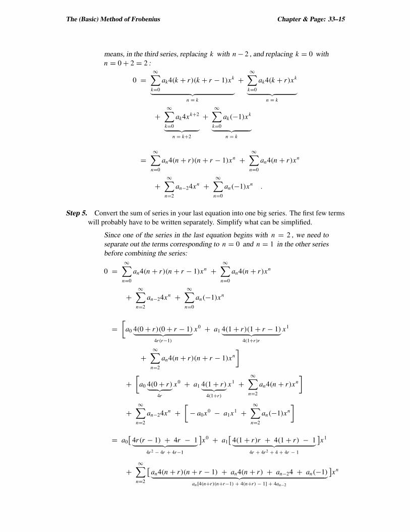
The (Basic) Method of Frobenius Chapter & Page: 33–15
means, in the third series, replacing k with n − 2 , and replacing k = 0 with
n = 0 + 2 = 2 :
0 =∞
∑
k=0
ak4(k + r)(k + r − 1)xk
︸ ︷︷ ︸
n = k
+∞
∑
k=0
ak4(k + r)xk
︸ ︷︷ ︸
n = k
+∞
∑
k=0
ak4xk+2
︸ ︷︷ ︸
n = k+2
+∞
∑
k=0
ak(−1)xk
︸ ︷︷ ︸
n = k
=∞
∑
n=0
an4(n + r)(n + r − 1)xn +∞
∑
n=0
an4(n + r)xn
+∞
∑
n=2
an−24xn +∞
∑
n=0
an(−1)xn .
Step 5. Convert the sum of series in your last equation into one big series. The first few terms
will probably have to be written separately. Simplify what can be simplified.
Since one of the series in the last equation begins with n = 2 , we need to
separate out the terms corresponding to n = 0 and n = 1 in the other series
before combining the series:
0 =∞
∑
n=0
an4(n + r)(n + r − 1)xn +∞
∑
n=0
an4(n + r)xn
+∞
∑
n=2
an−24xn +∞
∑
n=0
an(−1)xn
=[
a0 4(0 + r)(0 + r − 1)︸ ︷︷ ︸
4r(r−1)
x0 + a1 4(1 + r)(1 + r − 1)︸ ︷︷ ︸
4(1+r)r
x1
+∞
∑
n=2
an4(n + r)(n + r − 1)xn
]
+[
a0 4(0 + r)︸ ︷︷ ︸
4r
x0 + a1 4(1 + r)︸ ︷︷ ︸
4(1+r)
x1 +∞
∑
n=2
an4(n + r)xn
]
+∞
∑
n=2
an−24xn +[
− a0x0 − a1x1 +∞
∑
n=2
an(−1)xn
]
= a0
[
4r(r − 1) + 4r − 1︸ ︷︷ ︸
4r2 − 4r + 4r−1
]
x0 + a1
[
4(1 + r)r + 4(1 + r) − 1︸ ︷︷ ︸
4r + 4r2 + 4 + 4r − 1
]
x1
+∞
∑
n=2
[
an4(n + r)(n + r − 1) + an4(n + r) + an−24 + an(−1)︸ ︷︷ ︸
an [4(n+r)(n+r−1) + 4(n+r) − 1] + 4an−2
]
xn
Chapter & Page: 33–16 Modified Power Series Solutions and the Basic Method of Frobenius
= a0
[
4r 2 − 1]
x0 + a1
[
4r 2 + 8r + 3]
x1
+∞
∑
n=2
[
an
[
4(n + r)(n + r) − 1]
+ 4an−2
]
xn .
So our differential equation reduces to
a0
[
4r 2 − 1]
x0 + a1
[
4r 2 + 8r + 3]
x1
+∞
∑
n=2
[
an
[
4(n + r)2 − 1]
+ 4an−2
]
xn = 0 . (33.16)
Step 6. The first term in the last equation just derived will be of the form
a0
[
formula of r]
(x − x0)0 .
Since each term in the series must vanish, we must have
a0
[
formula of r]
= 0 .
Moreover, since a0 6= 0 (by assumption), the above must reduce to
formula of r = 0 .
This is the indicial equation for the differential equation. It will be a quadratic equation
(we’ll see why later). Solve this equation for r . You will get two solutions (sometimes
called either the exponents of the solution or the exponents of the singularity). Denote
them by r1 and r2 . If the exponents are real (which is common in applications), label
the exponents so that r1 ≥ r2 . If the exponents are not real, then it does not matter which
is labeled as r1 .10
In our example, the first term in the “big series” is the first term in equation
(33.16),
a0
[
4r 2 − 1]
x0 .
Since this must be zero (and a0 6= 0 by assumption) the indicial equation is
4r 2 − 1 = 0 . (33.17)
Thus,
r = ±√
1
4= ±1
2.
Following the convention given above (that r1 ≥ r2 ),
r1 = 1
2and r2 = −1
2.
10 We are assuming the coefficients of our differential equation— α , β and γ — are real-valued functions on the
real line. In the very unlikely case they are not, then a more general convention should be used: If the solutions to
the indicial equation differ by an integer, then label them so that r1 − r2 ≥ 0 . Otherwise, it does not matter which
you call r1 and which you call r2 . The reason for this convention will become apparent later (in section 33.5)
after we further discuss the formulas arising from the Frobenious method.
The (Basic) Method of Frobenius Chapter & Page: 33–17
Step 7. Using r1 (the largest r if the exponents are real):
(a) Plug r1 into the last series equation (and simplify, if possible). This will give you
an equation of the form
∞∑
n=n0
[
nth formula of a j ’s]
(x − x0)n = 0 .
Since each term must vanish, we must have
nth formula of a j ’s = 0 for n0 ≤ n .
(b) Solve this last set of equations for
ahighest index = formula of n and lower indexed a j ’s .
A few of these equations may need to be treated separately, but you will also
obtain a relatively simple formula that holds for all indices above some fixed value.
This formula is the recursion formula for computing each coefficient an from the
previously computed coefficients.
(c) (Optional) To simplify things just a little, do another change of indices so that the
recursion formula just derived is rewritten as
ak = formula of k and lower-indexed coefficients .
Letting r = r1 = 1/2 in equation (33.16) yields
0 = a0
[
4r 2 − 1]
x0 + a1
[
4r 2 + 8r + 3]
x1
+∞
∑
n=2
[
an
[
4(n + r)2 − 1]
+ 4an−2
]
xn
= a0
[
4(
1
2
)2
− 1
]
x0 + a1
[
4(
1
2
)2
+ 8(
1
2
)
+ 3
]
x1
+∞
∑
n=2
[
an
[
4(
n + 1
2
)2
− 1
]
+ 4an−2
]
xn
= a00x0 + a18x1 +∞
∑
n=2
[
an
[
4n2 + 4n]
+ 4an−2
]
xn .
The first term vanishes (as it should since r = 1/2 satisfies the indicial
equation, which came from making the first term vanish). Doing a little
more simple algebra, we see that, with r = 1/2 , equation (33.16) reduces
to
0a0x0 + 8a1x1 +∞
∑
n=2
4[
n(n + 1)an + an−2
]
xn = 0 . (33.18)
Chapter & Page: 33–18 Modified Power Series Solutions and the Basic Method of Frobenius
Since the individual terms in this series must vanish, we have
0a0 = 0 , 8a1 = 0
and
n(n + 1)an + an−2 = 0 for n = 2, 3, 4 . . . .
Solving for an gives us the recursion formula
an = −1
n(n + 1)an−2 for n = 2, 3, 4 . . . .
Using the trivial change of index, k = n , this is
ak = −1
k(k + 1)ak−2 for k = 2, 3, 4 . . . . (33.19)
(d) Use the recursion formula (and any corresponding formulas for the lower-order
terms) to find all the ak’s in terms of a0 and, possibly, one other am . Look for
patterns!
From the first two terms in equation (33.18),
0a0 = 0 H⇒ a0 is arbitrary.
8a1 = 0 H⇒ a1 = 0 .
Using these values and recursion formula (33.19) with k = 2, 3, 4, . . .
(and looking for patterns):
a2 = −1
2(2 + 1)a2−2 = −1
2 · 3a0 ,
a3 = −1
3(3 + 1)a3−2 = −1
3 · 4a1 = −1
3 · 4· 0 = 0 ,
a4 = −1
4(4 + 1)a4−2 = −1
4 · 5a2 = −1
4 · 5· −1
2 · 3a0 = (−1)2
5 · 4 · 3 · 2a0 = (−1)2
5!a0 ,
a5 = −1
5(5 + 1)a5−2 = −1
5 · 6· 0 = 0 ,
a6 = −1
6(6 + 1)a6−2 = −1
6 · 7a4 = −1
7 · 6· (−1)2
5!a0 = (−1)3
7!a0 ,
...
The patterns should be obvious here:
ak = 0 for k = 1, 3, 5, 7, . . . ,
and
ak = (−1)k/2
(k + 1)!a0 for k = 2, 4, 6, 8, . . . .
Using k = 2m , this can be written more conveniently as
a2m = (−1)m a0
(2m + 1)!for m = 1, 2, 3, 4, . . . .

The (Basic) Method of Frobenius Chapter & Page: 33–19
Moreover, this last equation reduces to the trivially true statement “ a0 =a0 ” if m = 0 . So, in fact, it gives all the even-indexed coefficients,
a2m = (−1)m a0
(2m + 1)!for m = 0, 1, 2, 3, 4, . . . .
(e) Using r = r1 along with the formulas just derived for the coefficients, write out
the resulting series for y . Try to simplify it and factor out the arbitrary constant(s).
Plugging r = 1/2 and the formulas just derived for the ak’s into the
formula originally assumed for y (equation (33.15) on page 33–13), we
get
y = xr
∞∑
k=0
ak xk
= xr
[ ∞∑
k=0k odd
ak xk +∞
∑
k=0k even
ak xk
]
= x1/2
[ ∞∑
k=0k odd
0 · xk +∞
∑
m=0
(−1)m a0
(2m + 1)!x2m
]
= x1/2
[
0 + a0
∞∑
m=0
(−1)m 1
(2m + 1)!x2m
]
.
So one set of solutions to Bessel’s equation of order 1/2 (equation (33.11)
on page 33–12) is given by
y = a0 x1/2
∞∑
m=0
(−1)m
(2m + 1)!x2m (33.20)
with a0 being an arbitrary constant.
Step 8. If the indical equation has two distinct solutions, now repeat step 7 with the other
exponent, r2 , replacing r1 .11 If r2 = r1 , just go to the next step.
Sometimes (but not always) this step will lead to a solution of the form
(x − x0)r2
∞∑
k=0
ak(x − x0)k .
with a0 being the only arbitrary constant. But sometimes this step leads to a series having
two arbitrary constants, with one being multiplied by the series solution already found in
the previous steps (our example will illustrate this). And sometimes this step leads to a
contradiction, telling you that there is no solution of the form
(x − x0)r2
∞∑
k=0
ak(x − x0)k with a0 6= 0 .
(We’ll discuss this further in Problems Possibly Arising in Step 8 starting on page 33–28.)
11 But first see Dealing with Complex Exponents starting on page 33–32 if the exponents are complex.
Chapter & Page: 33–20 Modified Power Series Solutions and the Basic Method of Frobenius
Letting r = r2 = −1/2 in equation (33.16) yields
0 = a0
[
4r 2 − 1]
x0 + a1
[
4r 2 + 8r + 3]
x1
+∞
∑
n=2
[
an
[
4(n + r)2 − 1]
+ 4an−2
]
xn
= a0
[
4(
−1
2
)2
− 1
]
x0 + a1
[
4(
−1
2
)2
+ 8(
−1
2
)
+ 3
]
x1
+∞
∑
n=2
[
an
[
4(
n − 1
2
)2
− 1
]
+ 4an−2
]
xn
= a00x0 + a10x1 +∞
∑
n=2
[
an
[
4n2 − 4n]
+ 4an−2
]
xn
That is,
0a0x0 + 0a1x1 +∞
∑
n=2
4[
ann(n − 1) + an−2
]
xn = 0 ,
which means that
0a0 = 0 , 0a1 = 0
and
ann(n − 1) + an−2 = 0 for n = 2, 3, 4, . . . .
This tells us that a0 and a1 can be any values (i.e., are arbitrary constants) and
that the remaining an’s can be computed from these two arbitrary constants
via the recursion formula
an = −1
n(n − 1)an−2 for n = 2, 3, 4, . . . .
That is,
ak = −1
k(k − 1)ak−2 for k = 2, 3, 4, . . . . (33.21)
Why don’t you finish these computations as an exercise? You should have no
trouble in obtaining
y = a0x−1/2
∞∑
m=0
(−1)m
(2m)!x2m + a1x−1/2
∞∑
m=0
(−1)m
(2m + 1)!x2m+1 . (33.22)
Note that the second series term is the same series (slightly rewritten) as in
equation (33.20) (since x−1/2x2m+1 = x1/2x2m ).
?◮Exercise 33.1: Do the computations left “as an exercise” in the last statement.
The (Basic) Method of Frobenius Chapter & Page: 33–21
Step 9. If the last step yielded y as an arbitrary linear combination of two different series, then
that is the general solution to the original differential equation. If the last step yielded
y as just one arbitrary constant times a series, then the general solution to the original
differential equation is the linear combination of the two series obtained at the end of
steps 7 and 8. Either way, write down the general solution (using different symbols for
the two different arbitrary constants!). If step 8 did not yield a new series solution, then
at least write down the one solution previously derived, noting that a second solution is
still needed for the general solution to the differential equation.
We are in luck. In the last step we obtained y as the linear combination of
two different series (equation (33.22)). So
y = a0x−1/2
∞∑
m=0
(−1)m
(2m)!x2m + a1x−1/2
∞∑
m=0
(−1)m
(2m + 1)!x2m+1 ,
is the general solution to our original differential equation (equation (33.11)
— Bessel’s equation of order 1/2 ).
Last Step. See if you recognize the series as the series for some well-known function (you
probably won’t!).
Our luck continues! The two power series in our last formula for y are easily
recognized as the Taylor series for the cosine and sine functions,
y = a0x−1/2
∞∑
m=0
(−1)m
(2m)!x2m + a1x−1/2
∞∑
m=0
(−1)m
(2m + 1)!x2m+1
= a0x−1/2 cos(x) + a1x−1/2 sin(x) .
So we can also write the general solution to Bessel’s equation of order 1/2 as
y = a0
cos(x)√
x+ a1
sin(x)√
x. (33.23)
“First” and “Second” Solutions
For purposes of discussion, it is convenient to refer to the first solution found in the basic method
of Frobenius,
y(x) = (x − x0)r1
∞∑
k=0
ak(x − x0)k ,
as the first solution. If we then pick a particular nonzero value for a0 , then we have a first
particular solution. In the above, our first solution was
y(x) = a0 x1/2
∞∑
m=0
(−1)m
(2m + 1)!x2m ,
Chapter & Page: 33–22 Modified Power Series Solutions and the Basic Method of Frobenius
Taking a0 = 1 , we then have a first particular solution
y1(x) = x1/2
∞∑
m=0
(−1)m
(2m + 1)!x2m .
Naturally, if we also obtain a solution corresponding to r2 in step 8,
y(x) = (x − x0)r2
∞∑
k=0
ak(x − x0)k ,
then we will refer to that as our second solution, with a second particular solution being this
with a specific nonzero value chosen for a0 and any specific value chosen for any other arbitrary
constant. For example, in illustrating the basic method of Frobenious, we obtained
y(x) = a0x−1/2
∞∑
m=0
(−1)m
(2m)!x2m + a1x−1/2
∞∑
m=0
(−1)m
(2m + 1)!x2m+1
as our second solution. Choosing a0 = 1 and a1 = 0 , we get the second particular solution
y2(x) = x−1/2
∞∑
m=0
(−1)m
(2m)!x2m .
While we are at it, let us agree that, for the rest of this chapter, x0 always denotes a regular
singular point for some differential equation of interest, and that r1 and r2 always denote the
corresponding exponents; that is, the solutions to the corresponding indicial equation. Let us
further agree that these exponents are indexed according to the convention given in the basic
Frobenious, with r1 ≥ r2 if they are real.
33.4 Basic Notes on Using the Frobenius MethodThe Obvious
One thing should be obvious: The method we’ve just outlined is even longer and more tedious
than the algebraic method used in chapter 31 to find power series solutions to similar equations
about ordinary points. On the other hand, much of this method is based on that algebraic method,
which, by now, you have surely mastered.
Naturally, all the ‘practical advice’ given regarding the algebraic method in chapter 31 still
holds, including the recommendation that you use
Y (X) = y(x) with X = x − x0
to simplify your calculations when x0 6= 0 .
But there are a number of other things you should be aware of:
Basic Notes on Using the Frobenius Method Chapter & Page: 33–23
Solutions on Intervals with x < x0
On an interval with x < x0 , (x − x0)r might be complex-valued (or even ambiguous) if r is
not an integer. For example,
(x − x0)1/2 = (− |x − x0|)
1/2 = (−1)1/2 |x − x0|
1/2 = ±i |x − x0|1/2 .
More generally, we will have
(x − x0)r = (− |x − x0|)r = (−1)r |x − x0|r when x < x0 .
But this is not a significant issue because (−1)r can be viewed as a constant (possibly complex)
and can be divided out of the final formula (or incorporated in the arbitrary constants). Thus, in
our final formulas for y(x) , we can replace
(x − x0)r with |x − x0|r .
to avoid having any explicitly complex-valued expressions (at least when r is not complex).
Let’s keep in mind that this is only needed if r is not an integer.
Convergence of the Series
It probably won’t surprise you to learn that the Frobenius radius of analyticity serves as a lower
bound on the radius of convergence for the power series found in the Frobenius method. To be
precise, we have the following theorem:
Theorem 33.3
Let x0 be a regular singular point for some second-order homogeneous linear differential equation
a(x)y′′ + b(x)y′ + c(x)y = 0
and let
y(x) = |x − x0|r∞
∑
k=0
ak(x − x0)k
be a modified power series solution to the differential equation found by the basic method of
Frobenius. Then the radius of convergence for∑∞
k=0 ak(x −x0)k is at least equal to the Frobenius
radius of convergence about x0 for this differential equation.
We will verify this claim in chapter 35. For now, let us simply note that this theorem assures
us that the given solution y is valid at least on the intervals
(x0 − R, x0) and (x0, x0 + R)
where R is that Frobenious radius of convergence. Whether or not we can include the point x0
depends on the value of the exponent r .
!◮Example 33.6: To illustrate the Frobenius method, we found modified power series solutions
about x0 = 0
y1(x) = x1/2
∞∑
m=0
(−1)m
(2m + 1)!x2m and y2(x) = x−1/2
∞∑
m=0
(−1)m
(2m)!x2m
Chapter & Page: 33–24 Modified Power Series Solutions and the Basic Method of Frobenius
for Bessel’s equation of order 1/2 ,
y′′ + 1
xy′ +
[
1 − 1
4x2
]
y = 0 .
Since there are no singular points for this differential equation other than x0 = 0 , the Frobenius
radius of convergence for this differential equation about x0 = 0 is R = ∞ . That means the
power series in the above formulas for y1 and y2 converge everywhere.
However, the x1/2 and x−1/2 factors multiplying these power series are not “well be-
haved” at x0 = 0 — neither is differentiable there, and one becomes infinite as x → 0 . So,
the above formulas for y1 and y2 are valid only on intervals not containing x = 0 , the largest
of which are (0,∞) and (−∞, 0) . Of course, on (−∞, 0) the square roots yield imaginary
values, and we would prefer using the solutions
y1(x) = |x |1/2∞
∑
m=0
(−1)m
(2m + 1)!x2m and y2(x) = |x |−1/2
∞∑
m=0
(−1)m
(2m)!x2m .
Variations of the Method
Naturally, there are several variations of “the basic method of Frobenius”. The one just given is
merely one the author finds convenient for initial discussion.
One variation you may want to consider is to find particular solutions without arbitrary
constants by setting “ a0 = 1 ”. That is, in step 1, assume
y(x) = (x − x0)r
∞∑
k=0
ak(x − x0)k with a0 = 1 .
Assuming a0 is 1 , instead of an arbitrary nonzero constant, leads to a first particular solution
y1(x) = (x − x0)r1
∞∑
k=0
ak(x − x0)k with a0 = 1 .
With a little thought, you will realize that this is exactly the same as you would have obtained at
the end of step 7, only not multiplied by an arbitrary constant. In particular, had we done this
with the Bessel’s equation used to illustrate the method, we would have obtained
y1(x) = x1/2
∞∑
m=0
(−1)m
(2m + 1)!x2m
instead of formula (33.20) on page 33–19.
If r2 6= r1 , then, with luck, doing step 8 will yield a second particular solution
y2(x) = (x − x0)r2
∞∑
k=0
ak(x − x0)k with a0 = 1 .
As mentioned, one of the ak’s other than a0 may also be arbitrary. Set that equal to your favorite
number for computation, 0 . In particular, doing this with the illustrating example would have
yielded
y2(x) = x−1/2
∞∑
m=0
(−1)m
(2m)!x2m ,
About the Indicial and Recursion Formulas Chapter & Page: 33–25
instead of formula (33.22) on page 33–20.
Assuming the second particular solution can be found, this variant of the method yields a pair
of particular solutions {y1, y2} that, because r1 6= r1 , is easily seen to be linearly independent
over any interval on which the formulas are valid. Thus,
y(x) = c1 y1(x) + c2 y2(x)
is the general solution to the differential equation over this interval.
Using the Method When x0 is an Ordinary Point
It should be noted that we can also find the power series solutions of a differential equation about
an ordinary point x0 using the basic Frobenius method (ignoring, of course, the first preliminary
step). In practice, though, it would be silly to go through the extra work in the Frobenius method
when you can use the shorter algebraic method from chapter 31. After all, if x0 is an ordinary
point for our differential equation, then we already know the solution y can be written as
y(x) = a0 y1(x) + a1 y2(x)
where y1(x) and y2(x) are power series about x0 with
y1(x) = 1 + a summation of terms of order 2 or more
= (x − x0)0
∞∑
k=0
bk(x − x0)k with bk = 1
and
y2(x) = 1 · (x − x0) + a summation of terms of order 2 or more
= (x − x0)1
∞∑
k=0
ck(x − x0)k with ck = 1
(see Initial-Value Problems on page 31–24). Clearly then, r2 = 0 and r1 = 1 , and the indicial
equation that would arise in using the Frobenius method would just be r(r − 1) = 0 .
So why bother solving for the exponents r1 and r2 of a differential equation at a point x0
when you don’t need to? It’s easy enough to determine whether a point x0 is an ordinary point
or a regular singular point for your differential equation. Do so, and don’t waste your time using
the Frobenius method unless the point in question is a regular singular point.
33.5 About the Indicial and Recursion Formulas
In chapter 35, we will closely examine the formulas involved in the basic Frobenius method.
Here are a few things regarding the indicial equation and the recursion formulas that we will
verify then (and which you should observe in your own computations now).
Chapter & Page: 33–26 Modified Power Series Solutions and the Basic Method of Frobenius
The Indicial Equation and the Exponents
Remember that one of the preliminary steps has us rewriting the differential equation as
(x − x0)2α(x)y′′ + (x − x0)β(x)y′ + γ (x)y = 0
where α , β and γ are polynomials, with α(x0) 6= 0 , and with no factors shared by all three.
In practice, these polynomials are almost always real (i.e., their coefficients are real numbers).
Let us assume this.
If you carefully follow the subsequent computations in the basic Frobenius method, you will
discover that the indicial equation is just as we suspected at the start of section 33.3; namely,
α0r(r − 1) + β0r + γ0 = 0 ,
where
α0 = α(x0) , β0 = β(x0) and γ0 = γ (x0) .
The exponents for our differential equation (i.e., the solutions to the indicial equation) can then
be found by rewriting the indicial equation as
α0r 2 + (β0 − α0)r + γ0 = 0
and using basic algebra.
!◮Example 33.7: In describing the Frobenius method, we used Bessel’s equation of order 1/2
with x0 = 0 . That equation was (on page 33–13) rewritten as
4x2 y′′ + 4xy′ + [4x2 − 1]y = 0 ,
which is
(x − 0)2α(x)y′′ + (x − 0)β(x)y′ + γ (x)y = 0
with
α(x) = 4 , β(x) = 4 and γ (x) = 4x2 − 1 .
So
α0 = α(0) = 4 , β0 = β(0) = 4 and γ0 = γ (0) = −1 .
According to the above, the corresponding indicial equation should be
4r(r − 1) + 4r − 1 = 0 ,
which simplifies to
4r 2 − 1 = 0 ,
and which, indeed, is what we obtained (equation (33.17) on page 33–16) as the indicial
equation for Bessel’s equation of order 1/2 .
From basic algebra, we know that, if the coefficients of the indicial equation
α0r 2 + (β0 − α0)r + γ0 = 0
are all real numbers, then the two solutions to the indicial equation are either both real numbers
(possibly the same real numbers) or are complex conjugates of each other. This is usually the
case in practice (it is always the case in the examples and exercises of this chapter).
About the Indicial and Recursion Formulas Chapter & Page: 33–27
The Recursion Formulas
After finding the solutions r1 and r2 to the indicial equation, the basic method of Frobenius
has us deriving the recursion formula corresponding to each of these r ’s . In chapter 35, we’ll
discover that each of these recursion formulas can always be written as
ak = F(k, r, a0, a1, . . . , ak−1)
(k + r − r1) (k + r − r2)for k ≥ κ (33.24a)
where κ is some positive integer, and r is either r1 or r2 , depending on whether this is the
recursion formula corresponding to r1 or r2 , respectively. It also turns out that this formula is
derived from the seemingly equivalent relation
(k + r − r1) (k + r − r2) ak = F(k, r, a0, a1, . . . , ak−1) , (33.24b)
which holds for every integer k greater than or equal to κ . (This later equation will be useful
when we discuss possible “degeneracies” in the recursion formula).
At this point, all you need to know about F(k, r, a0, a1, . . . , ak−1) is that it is a formula that
yields a finite value for every possible choice of its variables. Unfortunately, it is not that easily
described, nor would knowing it be all that useful at this point.
Of greater interest is the fact that the denominator in the recursion formula factors so simply
and predicably. The recursion formula obtained using r = r1 will be
ak = F(k, r1, a0, a1, . . . , ak−1)
(k + r1 − r1)(k + r1 − r2)= F(k, r1, a0, a1, . . . , ak−1)
k(k + r1 − r2),
while the recursion formula obtained using r = r2 will be
ak = F(k, r2, a0, a1, . . . , ak−1)
(k + r2 − r1)(k + r2 − r2)= F(k, r2, a0, a1, . . . , ak−1)
(k − [r1 − r2])k.
!◮Example 33.8: In solving Bessel’s equation of order 1/2 we obtained
r1 = 1
2and r2 = −1
2.
The recursion formulas corresponding to each of these were found to be
ak = −1
k(k + 1)ak−2 and ak = −1
k(k − 1)ak−2 for k = 2, 3, 4, . . . ,
respectively (see formulas (33.19) and (33.21)). Looking at the recursion formula correspond-
ing to r = 1/2 we see that, indeed,
ak = −1
k(k + 1)ak−2 = −1
k(
k + 1
2−
[
−1
2
])ak−2 = −1
k (k + r1 − r2)ak−2 .
Likewise, looking at the recursion formula corresponding to r = 1/2 we see that
ak = −1
(k − 1)kak−2 = −1
(
k +[
−1
2
]
− 1
2
)
k
ak−2 = −1
(k + r2 − r1)kak−2 .
Knowing that the denominator in your recursion formulas should factor into either
k(k + r1 − r2) or (k + r2 − r1)k
should certainly simplify your factoring of that denominator! And if your denominator does not
so factor, then you know you made an error in your computations. So it provides a partial error
check.
It also leads us to our next topic.
Chapter & Page: 33–28 Modified Power Series Solutions and the Basic Method of Frobenius
Problems Possibly Arising in Step 8
In discussing step 8 of the basic Frobenius method, we indicated that there may be “problems” in
finding a modified series solution corresponding to r2 . Well, take a careful look at the recursion
formula obtained using r2 :
ak = F(k, r2, a0, a1, . . . , ak−1)
(k − [r1 − r2])kfor k ≥ κ
(remember, κ is some positive integer). See the problem? That’s correct, the denominator may
be zero for one of the k’s . And it occurs if (and only if) r1 and r2 differ by some integer K
greater than or equal to κ ,
r1 − r2 = K .
Then, when we attempt to compute aK , we get
aK = F(K , r2, a0, a1, . . . , ak−1)
(K − [r1 − r2])K
= F(K , r2, a0, a1, . . . , ak−1)
(K − K )K= F(K , r2, a0, a1, . . . , ak−1)
0!
Precisely what we can say about aK when this happens depends on whether the numerator in
this expression is zero or not. To clarify matters slightly, let’s rewrite the above using recursion
relation (33.24b) which, in this case, reduces to
0 · aK = F(K , r2, a0, a1, . . . , ak−1) (33.25)
Now:
1. If F(K , r2, a0, a1, . . . , ak−1) 6= 0 , then the recursion formula “blows up” at k = K ,
aK = F(K , r2, a0, a1, . . . , ak−1)
0,
More precisely, aK must satisfy
0 · aK = F(K , r2, a0, a1, . . . , ak−1) 6= 0 ,
which is impossible. Hence, it is impossible for our differential equation to have a solution
of the form (x − x0)r2
∑∞k=0 ak(x − x0)
k with a0 6= 0 .
2. If F(K , r2, a0, a1, . . . , ak−1) = 0 , then the recursion equation for aK reduces to
aK = 0
0,
an indeterminant expression telling us nothing about aK . More precisely, (33.25) reduces
to
0 · aK = 0 ,
which is valid for any value of aK ; that is, aK is another arbitrary constant (in addition
to a0 ). Moreover, a careful analysis will confirm that, in this case, we will re-derive the
modified power series solution corresponding to r1 with aK being the arbitrary constant
in that series solution.
About the Indicial and Recursion Formulas Chapter & Page: 33–29
But why don’t we worry about the denominator in the recursion formula obtained using r1 ,
ak = F(k, r1, a0, a1, . . . , ak−1)
k(k + r1 − r2)for k ≥ κ ?
Because this denominator is zero only if r1 −r2 is some negative integer, contrary to our labeling
convention of r1 ≥ r2 .
!◮Example 33.9: Consider
2xy′′ − 4y′ − y = 0 .
Multiplying this out by x we get it into the form
2x2 y′′ − 4xy′ − xy = 0 .
As noted in example 33.5 on page 33–10, this equation has one regular singular point,
x0 = 0 . Setting
y = y(x) = xr
∞∑
k=0
ak xk =∞
∑
k=0
ak xk+r
and differentiating, we get (as before)
y′ = d
dx
∞∑
k=0
ak xk+r =∞
∑
k=0
ak(k + r)xk+r−1
and
y′′ = d2
dx2
∞∑
k=0
ak xk+r =∞
∑
k=0
ak(k + r)(k + r − 1)xk+r−2 .
Plugging these into our differential equation:
0 = 2x2 y′′ − 4xy′ − xy
= 2x2
∞∑
k=0
ak(k + r)(k + r − 1)xk+r−2 − 4
∞∑
k=0
ak(k + r)xk+r−1 − x
∞∑
k=0
ak xk+r
=∞
∑
k=0
2ak(k + r)(k + r − 1)xk+r −∞
∑
k=0
4ak(k + r)xk+r −∞
∑
k=0
ak xk+r+1 .
Dividing out the xr , reindexing, and grouping like terms:
0 =∞
∑
k=0
2ak(k + r)(k + r − 1)xk
︸ ︷︷ ︸
n = k
−∞
∑
k=0
4ak(k + r)xk
︸ ︷︷ ︸
n = k
−∞
∑
k=0
ak xk+1
︸ ︷︷ ︸
n = k+1
=∞
∑
n=0
2an(n + r)(n + r − 1)xn −∞
∑
n=0
4an(n + r)xn −∞
∑
n=1
an xn
Chapter & Page: 33–30 Modified Power Series Solutions and the Basic Method of Frobenius
= 2a0(0 + r)(0 + r − 1)x0 +∞
∑
n=1
2an(n + r)(n + r − 1)xn
− 4a0(0 + r)x0 −∞
∑
n=1
4an−1(n + r)xn −∞
∑
n=1
an−1xn
= a0[2r(r − 1) − 4r︸ ︷︷ ︸
2r2−2r−4r
]x0 +∞
∑
n=1
{an[2(n + r)(n + r − 1) − 4(n + r)︸ ︷︷ ︸
2(n+r)(n+r−1−2)
] − an−1}xn .
Thus, our differential equation reduces to
a0
[
2(
r 2 − 3r)]
x0 +∞
∑
n=1
{an [2(n + r)(n + r − 3)] − an−1} xn = 0 . (33.26)
From the first term, we get the indicial equation:
2(
r 2 − 3r)
︸ ︷︷ ︸
2r(r−3)
= 0
So r can equal 0 or 3 . Since 3 > 0 , our convention has us identifying these solutions to
the indicial equation as
r1 = 3 and r2 = 0 .
Letting r = r1 = 3 in equation (33.26), we see that
0 = a0
[
2(
32 − 3 · 3)]
x0 +∞
∑
n=1
{an [2(n + 3)(n + 3 − 3)] − an−1} xn
= a0 [0] x0 +∞
∑
n=1
{an [2(n + 3)n] − an−1} xn
So, for n ≥ 1 ,
an [2(n + 3)n] − an−1 = 0 .
Solving for an , we obtain the recursion formula
an = 1
2n(n + 3)an−1 for n = 1, 2, 3, . . . .
Equivalently12,
ak = 1
2k(k + 3)ak−1 for k = 1, 2, 3, . . . .
Applying this recursion formula:
a1 = 1
2 · 1(1 + 3)a0 = 1
2 · 1(4)a0 ,
a2 = 1
2 · 2(2 + 3)a1 = 1
2 · 2(5)· 1
2 · 1(4)a0 = 1
22(2 · 1)(5 · 4)a0
= 3 · 2 · 1
22(2 · 1)(5 · 4 · 3 · 2 · 1)a0 = 6
22(2 · 1)(5 · 4 · 3 · 2 · 1)a0 ,
12 Observe that this is formula (33.24a) with κ = 1 and F(k, r1, a0, a1, . . . , ak−1) = 12
ak−1 .
About the Indicial and Recursion Formulas Chapter & Page: 33–31
a3 = 1
2 · 3(3 + 3)a2 = 1
2 · 3(6)· 6
22(2 · 1)(5 · 4 · 3 · 2 · 1)a0
= 6
23(3 · 2 · 1)(6 · 5 · 4 · 3 · 2 · 1)a0 ,
...
ak = 6
2k k!(k + 3)!a0 .
Notice that this last formula even holds for k = 0 and k = 1 . So
ak = 6
2k k!(k + 3)!a0 for k = 0, 1, 2, 3, . . . ,
and the corresponding modified power series solution is
y(x) = xr1
∞∑
k=0
ak xk = a0x3
∞∑
k=0
6
2k k!(k + 3)!xk .
Now let’s try to find a similar solution corresponding to r2 = 0 . Letting r = r2 = 0 in
equation (33.26) yields
0 = a0
[
2(
02 − 3 · 0)]
x0 +∞
∑
n=1
{an [2(n + 0)(n + 0 − 3)] − an−1} xn
= a0 [0] x0 +∞
∑
n=1
{an [2n(n − 3)] − an−1} xn .
So, for n ≥ 1 ,
an [2n(n − 3)] − an−1 = 0 .
Solving for an , we obtain the recursion formula
an = 1
2n(n − 3)an−1 for n = 1, 2, 3, . . . .
Applying this, we get
a1 = 1
2 · 1(1 − 3)a0 = 1
2 · 1(−2)a0 ,
a2 = 1
2 · 2(2 − 3)a1 = 1
2 · 2(−1)· 1
2 · 1(−2)a0 = 1
222 · 1(−1)(−2)a0 ,
a3 = 1
2 · 3(3 − 3)a1 = 1
2 · 2(0)· 1
222 · 1(−1)(−2)a0 = 1
0a0 !
In this case, the a3 “blows up” if a0 6= 0 . In other words, for this last equation to be true, we
must have
0 · a3 = a0 ,
contrary to our requirement that a0 6= 0 . So, for this differential equation, our search for a
solution of the form
xr
∞∑
k=0
ak xk with a0 6= 0
Chapter & Page: 33–32 Modified Power Series Solutions and the Basic Method of Frobenius
is doomed to failure when r = r2 . There is no such solution.
This leaves us with just the solutions found corresponding to r = r1 ,
y(x) = a0x3
∞∑
k=0
6
2k k!(k + 3)!xk .
In the next chapter, we will discuss how to find the complete general solution when, as in the
last example, the basic method of Frobenius does not yield a second solution. We’ll also finish
solving the differential equation in the last example.
33.6 Dealing with Complex Exponents
In practice, the exponents r1 and r2 are usually real numbers. Still, complex exponents are
possible. Fortunately, the differential equations arising from “real-world” problems usually have
real-valued coefficients, which means that, if r1 and r2 are not real valued, they will probably
be a conjugate pair
r1 = r+ = λ + iω and r2 = r− = λ − iω
with ω 6= 0 . In this case, step 7 of the Frobenius method (with r1 = r+ , and renaming a0 as
c+ ) leads to a solution of the form
y(x) = c+y+(x)
where
y+(x) = (x − x0)λ+iω
∞∑
k=0
αk(x − x0)k
with α0 = 1 . The other αk’s will be determined from the recursion formula and will simply be
the ak’s described in the method with a0 factored out. And they will probably be complex-valued
since the recursion formula probably involves r+ = λ + iω .
We could then continue with step 8 and compute the general series solution corresponding
to r2 = r− . Fortunately, this lengthy set of computations is completely unnecessary because you
can easily confirm that the complex conjugate y∗ of any solution y to our differential equation
is another solution to our differential equation (see exercise 33.7 on page 33–38). Thus, as a
“second solution”, we can just use
y−(x) =[
y+(x)]∗ =
[
(x − x0)λ+iω
∞∑
k=0
αk(x − x0)k
]∗
= (x − x0)λ−iω
∞∑
k=0
αk∗(x − x0)
k .
It is also easy to verify that {y+(x), y−(x)} is linearly independent. Hence,
y(x) = c+y+(x) + c−y−(x)

Appendix: On Tests for Regular Singular Points Chapter & Page: 33–33
is a general solution to our differential equation.
However, the two solutions, y+ and y− will be complex valued. To avoid complex-valued
solutions, let’s employ the trick used before to derive a corresponding linearly independent pair
{y1, y2} of real-valued solutions to our differential equation by setting
y1(x) = 1
2
[
y+(x) + y−(x)]
and y2(x) = 1
2i
[
y+(x) − y−(x)]
.
Using the fact that
Xλ±iω = Xλ X iω = Xλ[
cos(ω ln |X |) ± i sin(ω ln |X |)]
,
it is a simple exercise to verify that
y1(x) = (x − x0)λ cos(ω ln |x − x0|)
∞∑
k=0
bk(x − x0)k
and
y2(x) = (x − x0)λ sin(ω ln |x − x0|)
∞∑
k=0
ck(x − x0)k
where the bk’s and ck’s are real-valued constants related to the above αk’s by
bk = αk + αk∗
2and ck = αk − αk
∗
2i.
33.7 Appendix: On Tests for Regular Singular PointsProof of Theorem 33.2
The validity of theorem 33.2 follows immediately from lemma 33.1 (which we’ve already proven)
and the next lemma.
Lemma 33.4
Let a , b and c be rational functions, and assume x0 is a singular point on the real line for
a(x)y′′ + b(x)y′ + c(x)y = 0 . (33.27)
If the two limits
limx→x0
(x − x0)b(x)
a(x)and lim
x→x0
(x − x0)2 c(x)
a(x)
are both finite values, then the differential equation can be written in quasi-Euler form
(x − x0)2α(x)y′′ + (x − x0)β(x)y′ + γ (x)y = 0
where α , β and γ are polynomials with α(x0) 6= 0 .
PROOF: Because a , b and c are rational functions (i.e., quotients of polynomials), we
can multiply equation (33.27) through by the common denominators, obtaining a differential

Chapter & Page: 33–34 Modified Power Series Solutions and the Basic Method of Frobenius
equation in which all the coefficients are polynomials. Then factoring out the (x − x0)-factors,
and dividing out the factors common to all terms, we obtain
(x − x0)k A(x)y′′ + (x − x0)
m B(x)y′ + (x − x0)nC(x)y = 0 (33.28)
where A , B an C are polynomials with
A(x0) 6= 0 , B(x0) 6= 0 and C(x0) 6= 0 ,
and k , m and n are nonnegative integers, one of which must be zero. Moreover, since this is
just a rewrite of equation (33.27), and x0 is, by assumption, a singular point for this differential
equation, we must have that k ≥ 1 . Hence m = 0 or n = 0 .
Dividing equations (33.27) and (33.28) by their leading terms then yields, respectively,
y′′ + b(x)
a(x)y′ + c(x)
a(x)y = 0
and
y′′ + (x − x0)m−k B(x)
A(x)y′ + (x − x0)
n−k C(x)
A(x)y = 0 .
But these last two equations describe the same differential equation, and have the same first
coefficients. Consequently, the other coefficients must be the same, giving us
b(x)
a(x)= (x − x0)
m−k B(x)
A(x)and
c(x)
a(x)= (x − x0)
n−k C(x)
A(x).
Thus,
limx→x0
(x − x0)b(x)
a(x)= lim
x→x0
(x − x0)m+1−k B(x)
A(x)= lim
x→x0
(x − x0)m+1−k B(x0)
A(x0)
and
limx→x0
(x − x0)2 c(x)
a(x)= lim
x→x0
(x − x0)n+2−k C(x)
A(x)= lim
x→x0
(x − x0)n+2−k C(x0)
A(x0).
By assumption, though, these limits are finite, and for the limits on the right to be finite, the
exponents must be zero or larger. This, combined with the fact that k ≥ 1 means that k , m and
l must satisfy
m + 1 ≥ k ≥ 1 and n + 2 ≥ k ≥ 1 . (33.29)
But remember, m , n and k are nonnegative integers with m = 0 or n = 0 . That leaves us
with only three possibilities:
1. If m = 0 , then the first inequality in set (33.29) reduces to
1 ≥ k ≥ 1
telling us that k = 1 . Equation (33.28) then becomes
(x − x0)1 A(x)y′′ + B(x)y′ + (x − x0)
nC(x)y = 0 .
Muliplying through by x − x0 this becomes
(x − x0)2α(x)y′′ + (x − x0)β(x)y′ + γ (x)y = 0
where α , β and γ are the polynomials
α(x) = A(x) , β(x) = B(x) and γ (x) = (x − x0)n+1C(x) .

Appendix: On Tests for Regular Singular Points Chapter & Page: 33–35
2. If n = 0 , then the second inequality in set (33.29) reduces to
2 ≥ k ≥ 1 .
So k = 1 or k = 2 , giving us two options:
(a) If k = 1 , then equation (33.28) becomes
(x − x0)1 A(x)y′′ + (x − x0)
m B(x)y′ + C(x)y = 0 ,
which can be rewritten as
(x − x0)2α(x)y′′ + (x − x0)β(x)y′ + γ (x)y = 0
where α , β and γ are the polynomials
α(x) = A(x) , β(x) = (x−x0)m B(x) and γ (x) = (x−x0)C(x) .
(b) If k = 2 , then the other inequality inequality in set (33.29) becomes
m + 1 ≥ 2
Hence m ≥ 1 . In this case, equation (33.28) becomes
(x − x0)2 A(x)y′′ + (x − x0)
m B(x)y′ + C(x)y = 0
which is the same as
(x − x0)2α(x)y′′ + (x − x0)β(x)y′ + γ (x)y = 0
where α , β and γ are the polynomials
α(x) = A(x) , β(x) = (x−x0)m−1 B(x) and γ (x) = C(x) .
Note that, in each case, we can rewrite our differential equation as
(x − x0)2α(x)y′′ + (x − x0)β(x)y′ + γ (x)y = 0
where α , β and γ are polynomials with
α(x0) = α0(x0) 6= 0 .
So, in each case, we have rewritten our differential equation in quasi-Euler form, as claimed in
the lemma.
Testing for Regularity When the Coefficients Are NotRational
By using lemma 30.13 on page 30–21 on factoring analytic functions, or lemma 30.14 on page
30–22 on factoring quotients of analytic functions, you can easily modify the arguments in the

Chapter & Page: 33–36 Modified Power Series Solutions and the Basic Method of Frobenius
last proof to obtain an analog of the above lemma appropriate to differential equations whose
coefficients are not rational. Basically, just replace
“rational functions” with “quotients of functions analytic at x0 ” ,
and replace
“polynomials” with “functions analytic at x0 ” .
The resulting lemma, along with lemma 33.1, then yields the following analog to theorem 33.2.
Theorem 33.5 (testing for regular singular points (ver.2))
Assume x0 is a singular point on the real line for the differential equation
a(x)y′′ + b(x)y′ + c(x)y = 0
where a , b and c are quotients of functions analytic at x0 . Then x0 is a regular singular point
for this differential equation if and only if the two limits
limx→x0
(x − x0)b(x)
a(x)and lim
x→x0
(x − x0)2 c(x)
a(x)
are both finite values.
Additional Exercises
33.2. Find a fundamental set of solutions {y1, y2} for each of the following shifted Euler
equations, and sketch the graphs of y1 and y2 near the singular point.
a. (x − 3)2 y′′ − 2(x − 3)y′ + 2y = 0
b. (x − 1)2 y′′ − 5(x − 1)y′ + 9y = 0
c. 2x2 y′′ + 5xy′ + 1y = 0
d. (x + 2)2 y′′ + (x + 2)y′ = 0
e. 3(x − 5)2 y′′ − 4(x − 5)y′ + 2y = 0
f. (x − 5)2 y′′ + (x − 5)y′ + 4y = 0
33.3. Identify all of the singular points for each of the following differential equations, and
determine which of those on the real line are regular singular points, and which are
irregular singular points. Also, find the Frobenius radius of convergence R for the
given differential equation about the given x0 .
a. x2 y′′ + x
x − 2y′ + 2
x + 2y = 0 , x0 = 0
b. x3 y′′ + x2 y′ + y = 0 , x0 = 2
c.(
x3 − x4)
y′′ + (3x − 1)y′ + 827y = 0 , x0 = 1

Additional Exercises Chapter & Page: 33–37
d. y′′ + 1
x − 3y′ + 1
x − 4y = 0 , x0 = 3
e. y′′ + 1
(x − 3)2y′ + 1
(x − 4)2y = 0 , x0 = 4
f. y′′ +(
1
x− 1
3
)
y′ +(
1
x− 1
4
)
y = 0 , x0 = 0
g.(
4x2 − 1)
y′′ +(
4 − 2
x
)
y′ + 1 − x2
1 + x2y = 0 , x0 = 0
h.(
4 + x2)2
y′′ + y = 0 , x0 = 0
33.4. For each of the following differential equations, verify that x0 = 0 is a regular singular
point, and then use the basic method of Frobenius to find modified power series solutions.
In particular:
i Find and solve the corresponding indicial equation for the equation’s exponents
r1 and r2 .
ii Find the recursion formula corresponding to each exponent.
iii Find and explicitly write out at least the first four nonzero terms of all series
solutions about x0 = 0 that can be found by the basic Frobenius method (if a
series terminates, find all the nonzero terms).
iv Try to find a general formula for all the coefficients in each series.
v When a second particular solution cannot be found by the basic method, give a
reason that second solution cannot be found.
a. x2 y′′ − 2xy′ +(
x2 + 2)
y = 0
b. 4x2 y′′ + (1 − 4x)y = 0
c. x2 y′′ + xy′ + (4x − 4)y = 0
d.(
x2 − 9x4)
y′′ − 6xy′ + 10y = 0
e. x2 y′′ − xy′ + 1
1 − xy = 0
f. y′′ + 1
xy′ + y = 0 (Bessel’s equation of order 0 )
g. y′′ + 1
xy′ +
[
1 − 1
x2
]
y = 0 (Bessel’s equation of order 1 )
h. 2x2 y′′ +(
5x − 2x3)
y′ + (1 − x2)y = 0
i. x2 y′′ −(
5x + 2x2)
y′ + (9 + 4x) y = 0
j.(
3x2 − 3x3)
y′′ −(
4x + 5x2)
y′ + 2y = 0
k. x2 y′′ −(
x + x2)
y′ + 4xy = 0
l. 4x2 y′′ + 8x2 y′ + y = 0
Chapter & Page: 33–38 Modified Power Series Solutions and the Basic Method of Frobenius
m. x2 y′′ +(
x − x4)
y′ + 3x3 y = 0
n.(
9x2 + 9x3)
y′′ +(
9x + 27x2)
y′ + (8x − 1)y = 0
33.5. For each of the following, verify that the given x0 is a regular singular point for the
given differential equation, and then use the basic method of Frobenius to find modified
power series solutions to that differential equation. In particular:
i Find and solve the corresponding indicial equation for the equation’s exponents
r1 and r2 .
ii Find the recursion formula corresponding to each exponent.
iii Find and explicitly write out at least the first four nonzero terms of all series
solutions about x0 = 0 that can be found by the basic Frobenius method (if a
series terminates, find all the nonzero terms).
iv Try to find a general formula for all the coefficients in each series.
v When a second particular solution cannot be found by the basic method, give a
reason that second solution cannot be found.
a. (x − 3)y′′ + (x − 3)y′ + y = 0 , x0 = 3
b. y′′ + 2
x + 2y′ + y = 0 , x0 = −2
c. 4y′′ + 4x − 3
(x − 1)2y = 0 , x0 = 1
d. (x − 3)2 y′′ +(
x2 − 3x)
y′ − 3y = 0 , x0 = 3
33.6. Let∑∞
k=0 ak xk be a power series convergent on (−R, R) for some R > 0 . We already
know that, on (−R, R) ,
d
dx
∞∑
k=0
ak xk =∞
∑
k=0
d
dx
[
ak xk]
.
a. Using the above and the product rule confirm that, on (−R, R) ,
d
dx
[
xr
∞∑
k=0
ak xk
]
=∞
∑
k=0
ak(k + r)xk+r−1 .
for any real value r .
b. How does this justify the term-by-term differentiation used in step 2 of the basic
Frobenius method?
33.7. For the following, assume u and v are real-valued functions on some interval I , and
let y = u + iv .
Additional Exercises Chapter & Page: 33–39
a. Verify that
dy∗
dx=
(
dy
dx
)∗
andd2 y∗
dx2=
(
d2 y
dx2
)∗
where y∗ is the complex conjugate of y .
b. Further assume that, on some interval I , y satisfies
a(x)d2 y
dx2+ b(x)
dy
dx+ c(x)y = 0
where a , b and c are all real-valued functions. Using the results from the previous
part of this exercise, show that
a(x)d2 y∗
dx2+ b(x)
dy∗
dx+ c(x)y∗ = 0 .
Chapter & Page: 33–40 Modified Power Series Solutions and the Basic Method of Frobenius
Some Answers to Some of the Exercises
WARNING! Most of the following answers were prepared hastily and late at night. They
have not been properly proofread! Errors are likely!
2a. y1(x) = (x − 3)2 , y2(x) = x − 3
2b. y1(x) = (x − 1)3 , y2(x) = (x − 1)3 ln |x − 1|2c. y1(x) = x−1/2 , y2(x) = x−1
2d. y1(x) = 1 , y2(x) = ln |x + 2|2e. y1(x) = (x − 5)2 , y1(x) = 3
√x − 5
2f. y1(x) = cos(2 ln |x − 5|) , y1(x) = sin(2 ln |x − 5|)3a. Reg. sing. pts.: 0, 2, −2 ; No irreg. sing. pt. ; R = 2
3b. No Reg. sing. pt. ; Irreg. sing. pt.: 0 ; R = 2
3c. Reg. sing. pt.: 1 ; Irreg. sing. pt.: 0 ; R = 1
3d. Reg. sing. pt.: 3, 4 ; No irreg. sing. pt. ; R = 1
3e. Reg. sing. pt.: 4 ; Irreg. sing. pt.: 3 ; R = 1
3f. Reg. sing. pt.: 0 ; No irreg. sing. pt. ; R = ∞3g. Reg. sing. pts.: 0,
1
2, −1
2, i, −i ; No irreg. sing. pts. ; R = 1
23h. Reg. sing. pts.: 2i, −2i ; No irreg. sing. pt. ; R = 2
4a. r 2 − 3r + 2 = 0 ; r1 = 2 , r2 = 1 ;
For r = r1 , a1 = 0 , ak = −1
(k + 1)kak−2 ; y(x) = ay1(x) with
y1(x) = x2[
1 − 1
3!x2 + 1
5!x4 − 1
7!x6 − · · ·
]
= x2
∞∑
m=0
(−1)m
(2m + 1)!x2m = x sin(x)
For r = r2 , a1 = 0; ak = −1
k(k − 1)ak−2 ; y(x) = ay2(x) with
y2(x) = x[
1 − 1
2!x2 + 1
4!x4 − 1
6!x6 + · · ·
]
= x
∞∑
m=0
(−1)m
(2m)!x2m = x cos(x)
4b. 4r 2 − 4r + 1 = 0 ; r1 = r2 = 1
2;
For r = r1 : ak = 1
k2ak−1 ; y(x) = ay1(x) with
y1(x) =√
x
∞∑
k=0
1
(k!)2xk
No “second” value of r
4c. r 2 − 4 = 0 ; r1 = 2 , r2 = −2 ;
For r = r1 : ak = −4
k(k + 4)ak−1 ; y(x) = ay1(x) with
y1(x) = x2
[
1 − 4
5x + 42
(2)(6 · 5)x2 − 43
(3 · 2)(7 · 6 · 5)x3 + · · ·
]
= x2
∞∑
k=0
(−4)k4!k!(k + 4)!
xk
For r = r2 , the recursion formula blows up
4d. r 2 − 7r + 10 = 0 ; r1 = 5 , r2 = 2 ;
For r = r1 , a1 = 0 , ak = 9(k + 2)
kak−2 ; y(x) = ay1(x) with
y1(x) = x2
[
1 + 9 · 4
2x2 + 92 · 6
2x4 + 93 · 8
2x6 − · · ·
]
= x5
∞∑
m=0
9m(m + 1)x2m
For r = r2 , a1 = 0; ak = 9(k − 1)
k − 3ak−2 ; y(x) = ay2(x) with
Additional Exercises Chapter & Page: 33–41
y2(x) = x2[
1 − 9x2 − 3 · 92x4 − 5 · 93x6 + · · ·]
= x2
∞∑
m=0
9m(1 − 2m)x2m
4e. r 2 − 2r + 1 = 0 ; r1 = r2 = 1 ;
For r = r1 : ak = k − 2
kak−1 ; y(x) = ay1(x) with
y1(x) = x − x2
No “second” value of r
4f. r 2 = 0 ; r1 = r2 = 0 ;
For r = r1 : a1 = 0 , ak = −1
k2ak−2 ; y(x) = ay1(x) with
y1(x) = 1 − 1
22x2 + 1
(2 · 4)2x4 − 1
(6 · 4 · 2)2x6 + · · · =
∞∑
m=0
(−1)m
(2mm!)2x2m
No “second value” for r
4g. r 2 − 1 = 0 ; r1 = 1 , r2 = −1 ;
For r = r1 : a1 = 0 , ak = −1
k(k + 2)ak−2 ; y(x) = ay1(x) with
y1(x) = x[
1 − 1
2 · 4x2 + 1
(4 · 2)(6 · 4)x4 − 1
(6 · 4 · 2)(8 · 6 · 4)x6 + · · ·
]
= x
∞∑
m=0
(−1)m
22mm!(m + 1)!x2m
For r = r2 , the recursion formula blows up
4h. 2r 2 + 3r + 1 = 0 ; r1 = −1/2 , r2 = −1 ;
For r = r1 : a1 = 0 , ak = 2(k − 2)
k(2k + 1)ak−2 ; y(x) = ay1(x) with
y1(x) = x−1/2
For r = r2 : a1 = 0 , ak = 2k − 5
k(2k − 1)ak−2 ; y(x) = ay2(x) with
y2(x) = x−1[
1 − 1
2 · 3x2 − 1
4 · 2 · 7x4 − 1
6 · 4 · 2 · 11x6 + · · ·
]
= x−1
∞∑
m=0
−1
2mm!(4m − 1)x2m
4i. r 2 − 6r + 9 = 0 ; r1 = r2 = 3 ;
For r = r1 : ak = 2
kak−1 ; y(x) = ay1(x) with
y1(x) = x3
[
1 + 2
1x + 22
2x2 + 23
3 · 2x3 + · · ·
]
= x3
∞∑
k=0
2k
k!xk = x3e2x
No “second” value of r
4j. 3r 2 − 7r + 2 = 0 ; r1 = 2 , r2 = 1/3 ;
For r = r1 : ak = k + 1
kak−1 ; y(x) = ay1(x) with
y1(x) = x2[
1 + 2x + 3x2 + 4x3 + · · ·]
= x2
∞∑
k=0
(k + 1)xk
For r = r2 : ak = 3k − 2
3k − 5ak−1 ; y(x) = ay1(x) with
y1(x) = 3√
x[
1 − 1
2x − 4
2x2 − 7
2x3 + · · ·
]
= 3√
x
∞∑
k=0
2 − 3k
2xk
4k. r 2 − 2r = 0 ; r1 = 2 , r2 = 0 ;
For r = r1 : ak = k − 3
k(k + 2)ak−1 ; y(x) = ay1(x) with
y1(x) = x2 − 2
3x3 + 1
12x4
For r = r2 , the recursion formula blows up
4l. 4r 2 − 4r + 1 = 0 ; r1 = r2 = 1/2 ;
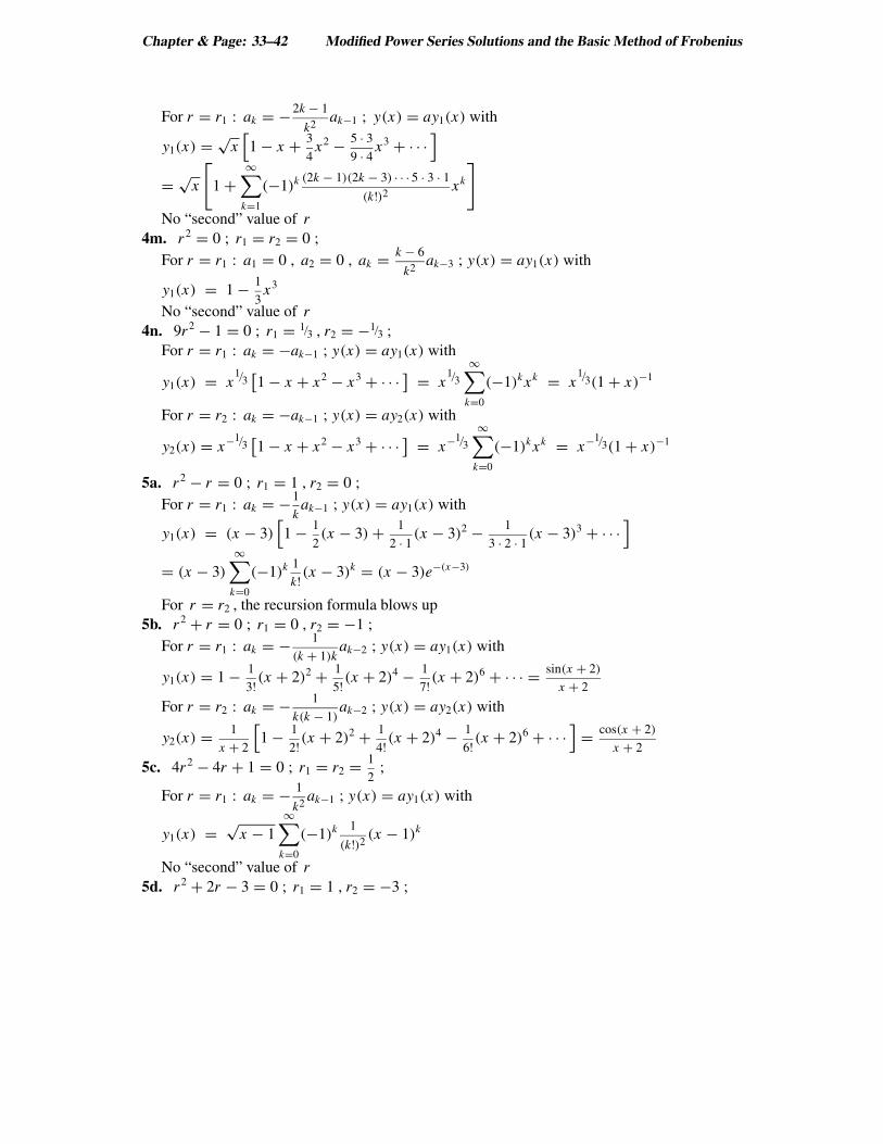
Chapter & Page: 33–42 Modified Power Series Solutions and the Basic Method of Frobenius
For r = r1 : ak = −2k − 1
k2ak−1 ; y(x) = ay1(x) with
y1(x) =√
x[
1 − x + 3
4x2 − 5 · 3
9 · 4x3 + · · ·
]
=√
x
[
1 +∞
∑
k=1
(−1)k (2k − 1)(2k − 3) · · · 5 · 3 · 1
(k!)2xk
]
No “second” value of r
4m. r 2 = 0 ; r1 = r2 = 0 ;
For r = r1 : a1 = 0 , a2 = 0 , ak = k − 6
k2ak−3 ; y(x) = ay1(x) with
y1(x) = 1 − 1
3x3
No “second” value of r
4n. 9r 2 − 1 = 0 ; r1 = 1/3 , r2 = −1/3 ;
For r = r1 : ak = −ak−1 ; y(x) = ay1(x) with
y1(x) = x1/3
[
1 − x + x2 − x3 + · · ·]
= x1/3
∞∑
k=0
(−1)k xk = x1/3(1 + x)−1
For r = r2 : ak = −ak−1 ; y(x) = ay2(x) with
y2(x) = x−1/3[
1 − x + x2 − x3 + · · ·]
= x−1/3
∞∑
k=0
(−1)k xk = x−1/3(1 + x)−1
5a. r 2 − r = 0 ; r1 = 1 , r2 = 0 ;
For r = r1 : ak = −1
kak−1 ; y(x) = ay1(x) with
y1(x) = (x − 3)
[
1 − 1
2(x − 3) + 1
2 · 1(x − 3)2 − 1
3 · 2 · 1(x − 3)3 + · · ·
]
= (x − 3)
∞∑
k=0
(−1)k 1
k!(x − 3)k = (x − 3)e−(x−3)
For r = r2 , the recursion formula blows up
5b. r 2 + r = 0 ; r1 = 0 , r2 = −1 ;
For r = r1 : ak = − 1
(k + 1)kak−2 ; y(x) = ay1(x) with
y1(x) = 1 − 1
3!(x + 2)2 + 1
5!(x + 2)4 − 1
7!(x + 2)6 + · · · = sin(x + 2)
x + 2
For r = r2 : ak = − 1
k(k − 1)ak−2 ; y(x) = ay2(x) with
y2(x) = 1
x + 2
[
1 − 1
2!(x + 2)2 + 1
4!(x + 2)4 − 1
6!(x + 2)6 + · · ·
]
= cos(x + 2)
x + 2
5c. 4r 2 − 4r + 1 = 0 ; r1 = r2 = 1
2;
For r = r1 : ak = − 1
k2ak−1 ; y(x) = ay1(x) with
y1(x) =√
x − 1
∞∑
k=0
(−1)k 1
(k!)2(x − 1)k
No “second” value of r
5d. r 2 + 2r − 3 = 0 ; r1 = 1 , r2 = −3 ;
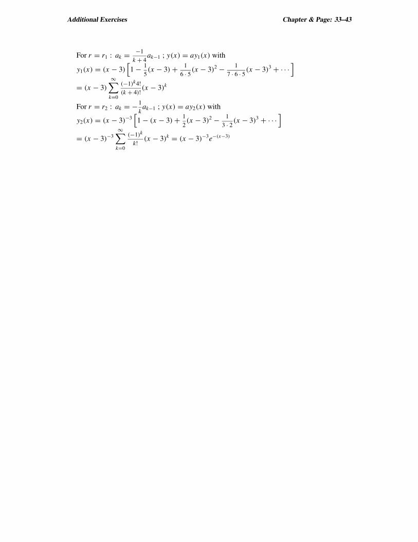
Additional Exercises Chapter & Page: 33–43
For r = r1 : ak = −1
k + 4ak−1 ; y(x) = ay1(x) with
y1(x) = (x − 3)[
1 − 1
5(x − 3) + 1
6 · 5(x − 3)2 − 1
7 · 6 · 5(x − 3)3 + · · ·
]
= (x − 3)
∞∑
k=0
(−1)k4!(k + 4)!
(x − 3)k
For r = r2 : ak = −1
kak−1 ; y(x) = ay2(x) with
y2(x) = (x − 3)−3[
1 − (x − 3) + 1
2(x − 3)2 − 1
3 · 2(x − 3)3 + · · ·
]
= (x − 3)−3
∞∑
k=0
(−1)k
k!(x − 3)k = (x − 3)−3e−(x−3)